LinSys2007 1

An (In)complete KalmanDecomposition for Uncertain Linear

Systems

An (In)complete KalmanDecomposition for Uncertain Linear

Systems

Ian R. Petersen †

† School of ITEE, University of New South Wales@ the Australian Defence Force Academy

LinSys2007 2

IntroductionIntroduction

� This paper considers the structure of uncertain linear systemsbuilding on concepts of “robust unobservability and “possiblecontrollibility”.

� One reason for considering the issue of observability for uncertainsystems might be to determine if a robust state estimator can beconstructed for the system. Similarly, one might consider the issueof controllability to determine if a robust state feedback controller forthe system.

� In this case, one would be interested in the question of whether thesystem is “observable” or “controllable” for all possible values of theuncertainty.

� The notions of controllability and observability are also central torealization theory. For example, it is known that if a linear timeinvariant system contains unobservable states or uncontrollable,those states can be removed in order to obtain a reduced dimensionrealization of the system’s input-output behavior.

LinSys2007 3

� For the case of uncertain systems when one is interested in theissue of “minimal realization”, a natural extension of this notion ofobservability is to consider robustly unobservable states which are“unobservable” for all possible values of the uncertainty.

� Similarly, a natural extension of the notion of controllability is toconsider “possibily controllable” states which are “controllable” forsome possible value of the uncertainty.

� We formally define these notions of robust unobservability andpossible controllability in terms of certain constrained optimizationproblems.

� We then apply the S-procedure to obtain conditions in terms ofunconstrained LQ optimal control problems dependent on Lagrangemultiplier parameters.

LinSys2007 4

� We then develop a geometric characterization for the set of robustlyunobservable states. We also (partially subject to some conditions)develop a geometric characterization of the set of possiblycontrollable states

� These characterizations imply that the set of robustly unobservablestates is in fact a linear subspace.

� Similarly (under some conditions), we show that the set of possiblycontrollable states is a linear subspace.

� These characterizations leads to a Kalman type decomposition forthe uncertain systems under consideration (provided the requiredconditions are satisfied).

LinSys2007 5

Problem FormulationProblem Formulation

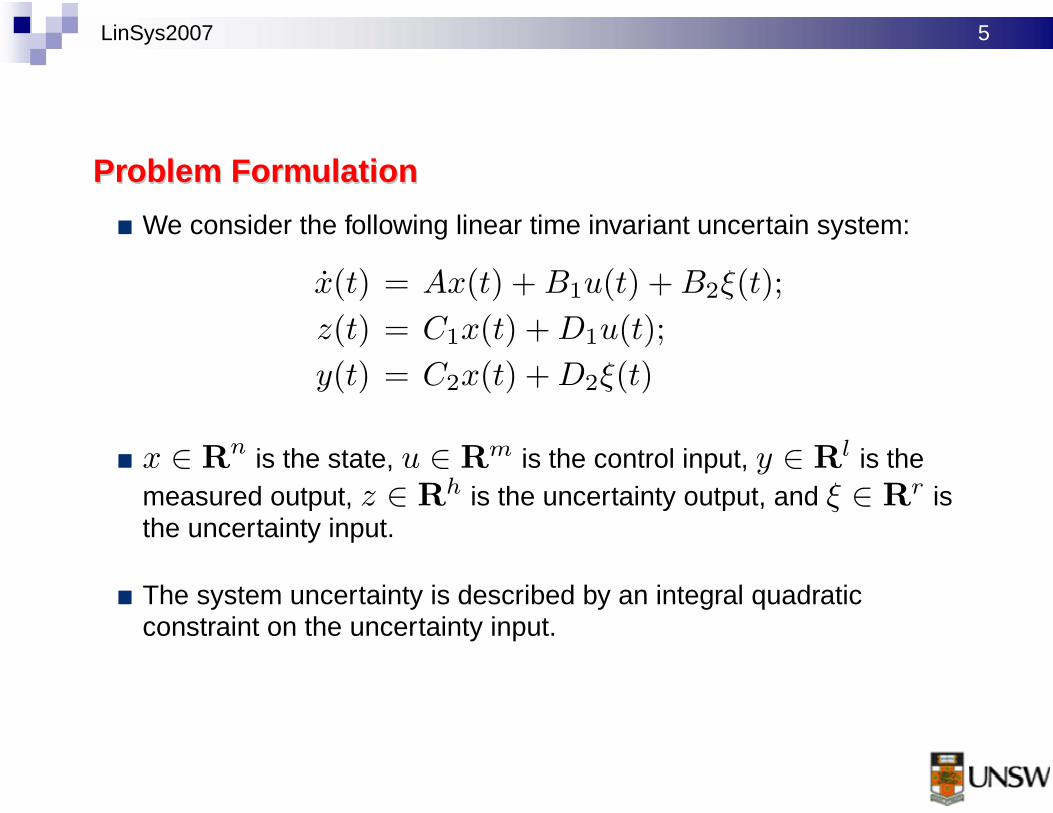
� We consider the following linear time invariant uncertain system:

x(t) = Ax(t) + B1u(t) + B2ξ(t);

z(t) = C1x(t) + D1u(t);

y(t) = C2x(t) + D2ξ(t)

� x ∈ Rn is the state, u ∈ R

m is the control input, y ∈ Rl is the

measured output, z ∈ Rh is the uncertainty output, and ξ ∈ R

r isthe uncertainty input.

� The system uncertainty is described by an integral quadraticconstraint on the uncertainty input.

LinSys2007 6

Integral Quadratic Constraint

� On a time interval [0, T ], we consider uncertainty inputsξ(·) ∈ L2[0, T ] such that for any control input u(·) ∈ L2[0, T ]and any corresponding solution x(·) to the system state equationsdefined on [0, T ], then ξ(·) ∈ L2[0, T ], and

∫ T

0

(

‖ξ(t)‖2 − ‖z(t)‖2)

dt ≤ d

where d > 0 is a given constant.

� The class admissible uncertainty inputs is denoted Ξ.

LinSys2007 7

The uncertain system can be represented by the following blockdiagram.

-

�

- -

∆(·)

u y

ξ z

NominalSystem

LinSys2007 8

� Our fundamental question:

� Given such an uncertain system model, can we construct asimpler uncertain system model with smaller state dimensions inthe state equations such that it will realize the same set ofinput-output behaviours as the original uncertain system model.

� The corresponding problem in linear systems theory is given astate space model, construct a state space model of smallerstate dimension (minimal realization) with the same transferfunction matrix.

� Based on an analogy with the linear time invariant systems result,our results provide a candidate method of achieving suchreduced order models for uncertain linear systems. Verificationthat our results in fact lead to these reduced dimensionrealizations for uncertain systems could be verified using someother results and is the subject of future research.

LinSys2007 9

Definition. The robust unobservability function for the above uncertainsystem on [0, T ] is defined as

Lo(x0, T )∆= sup

ξ(·)∈Ξ

∫ T

0

‖y(t)‖2dt

where x(0) = x0.

� This definition extends the standard definition of the observabilityGramian for linear time invariant systems.

LinSys2007 10

Notation.

D∆= {d ∈ R : d > 0}.

Definition. A non-zero state x0 ∈ Rn is said to be robustly unobserv-

able on [0, T ] ifinfd∈D

Lo(x0, T ) = 0.

A non-zero state x0 ∈ Rn is said to be (differentially) robustly unob-

servable if it is robustly unobservable on [0, T ] for all sufficiently smallT > 0.

The set of all differentially robustly unobservable states is referred to asthe robustly unobservable set U .

� The set U is analogous to the unobservable subspace in linear timeinvariant systems theory.

LinSys2007 11

Definition. The possible controllability function for the uncertain systemdefined on the time interval [0, T ] is defined as

Lc(x0, T )∆=

supǫ>0

infξ(·)∈Ξ

infu(·)∈L2[0,T ]

[

‖x(−T )‖2

ǫ+

∫ T

0‖u(t)‖2dt

]

where x(0) = x0.

� This definition extends the standard definition of the controllabilityGramian for linear time invariant systems.

� This definition is more complicated that the correspondingobservability definition due to the requirement to enforce a terminalcondition on the state.

LinSys2007 12

Definition. A non-zero state x0 ∈ Rn is said to be possibly controllable

on [0, T ] if

supd∈D

Lc(x0, T ) < ∞.

A non-zero state x0 ∈ Rn is said to be (differentially) possibly control-

lable if it is possibly controllable on [0, T ] for all sufficiently small T > 0.

The set of all differentially possibly controllable states is referred to as thepossibly controllable set C.

� The set C is analogous to the controllable subspace in linear timeinvariant systems theory.

LinSys2007 13

Optimal Control CharacterizationsOptimal Control Characterizations

� We can apply the S-procedure to provide characterizations of thepossibly controllable set and the robustly unobservable set in termsof certain LQ optimal control problems and corresponding Riccatidifferential equations.

LinSys2007 14

An Unconstrained Optimization Problem for RobustUnobservability

� We define a function Vτ (x0, T ) as follows:

Vτ (x0, T )∆= inf

ξ(·)∈L2[0,T ]

∫ T

0

(

−‖y‖2

+τ‖ξ‖2 − τ‖z‖2

)

dt.

� Here τ ≥ 0 is a given constant.

Observation. Note that by setting ξ(·) ≡ 0, we can see that

Vτ (x0, T ) ≤ 0 ∀τ ≥ 0.

Since Vτ (x0, T ) is the infimum of a collection of functions which areaffine linear in τ , then Vτ (x0, T ) must be a concave function of τ .

LinSys2007 15

Theorem. A state x0 ∈ Rn robustly unobservable on [0, T ] if and only

ifsupτ≥0

{Vτ (x0, T )} = 0

� We can calculate Vτ (x0, T ) by using a Riccati equation approachto solving the corresponding optimal control problem.

LinSys2007 16

Theorem. Let τ > 0 be given such that

τI − D′2D2 > 0.

ThenVτ (x0, T ) > −∞ ∀x0 ∈ R

n

if and only if the Riccati differential equation

−Q = A′Q + QA

−(QB2 − C ′2D2) [τI − D′

2D2]−1

(B′2Q − D′

2C2)

−C ′2C2 − τC ′

1C1;Q(T ) = 0

has a solution Qτ (t) defined on [0, T ]. In this case,

Vτ (x0, T ) = x′0Qτ (0)x0.

LinSys2007 17

A family of Unconstrained Optimal Control Problems for Poss ibleControllability

� For the uncertain system defined on the time interval [0, T ], wedefine functions W ǫ

τ (x0, T ) and Wτ (x0, T ) as follows for τ ≥ 0:

W ǫτ (x0, T )

∆= inf

[ξ(·),u(·)]∈L2[0,T ]

‖x(T )‖2

ǫ

+

∫ T

0

(

‖u‖2 + τ‖ξ‖2 − τ‖z‖2)

dt

subject to x(0) = x0;

Wτ (x0, T )∆= sup

ǫ>0W ǫ

τ (x0, T ).

� Again the controllability case is more complicated than theobservability case due to the terminal constraint on the state.

LinSys2007 18

Theorem. A non-zero state x0 ∈ Rn is possibly controllable on [0, T ]

if and only if

supǫ>0

supτ≥0

W ǫτ (x0, T ) = sup

τ≥0Wτ (x0, T ) < ∞

� We can calculate W ǫτ (x0, T ) by using a Riccati equation approach

to solving the corresponding optimal control problem.

LinSys2007 19

Theorem. Let τ > 0 be such that I − τD′1D1 > 0. Then

W ǫτ (x0, T ) > −∞ ∀x0 ∈ R

n

if and only if the Riccati differential equation

−P ǫ =

A′P ǫ + P ǫA

−(P ǫB1 − τC ′1D1) (I − τD′

1D1)−1

(P ǫB1 − τC ′1D1)

′

−P ǫB2B

′2P

ǫ

τ− τC1C

′1; P ǫ(T ) = I/ǫ

has a solution P ǫτ (t) defined on [0, T ]. In this case,

W ǫτ (x0, T ) = x′

0Pǫτ (0)x0.

LinSys2007 20

In order to calculate Wτ (x0, T ) we will also consider the followingRiccati Differential Equations:

Sǫ =ASǫ + SǫA′

−(B1 − τSǫC ′1D1) (I − τD′

1D1)−1

(B1 − τSǫC ′1D1)

′

−B2B

′2

τ− τSǫC1C

′1S

ǫ; Sǫ(T ) = ǫI;

S =AS + SA′

−(B1 − τSC ′1D1) (I − τD′

1D1)−1

(B1 − τSC ′1D1)

′

−B2B

′2

τ− τSC1C

′1S; S(T ) = 0

which are solved backwards in time.

LinSys2007 21

Theorem. Let τ > 0 be such that I−τD′1D1 > 0. Also suppose there

exists an ǫ0 > 0 such that for all ǫ ∈ (0, ǫ0), all non-zero x0 ∈ Rn then

W ǫτ (x0, T ) > 0. Then for any ǫ ∈ (0, ǫ0), the above Riccati equations

have solutions Sǫτ (t) > 0 and Sτ (t) ≥ 0 defined on [0, T ] and for any

x0 6= 0

W ǫτ (x0, T ) = x′

0 [Sǫτ (0)]

−1x0 > 0.

Also, if Sτ (0) > 0 then

Wτ (x0, T ) = x′0 [Sτ (0)]

−1x0 > 0.

Furthermore, if the matrix Sτ (0) ≥ 0 is singular and x0 is not containedwithin the range space of Sτ (0), then

Wτ (x0, T ) = ∞.

LinSys2007 22

Notes

� Although the result is useful in proving our results, it suffers from thedifficulty that the Riccati equation for Sτ may have a finite escapeeven if Wτ (x0, T ) remains finite.

� For all of the Riccati equations being considered, we can choose thetime interval [0, T ] sufficiently small to ensure that there exists asolution to the Riccati equation on that interval at least for a givenvalue of τ .

� The Riccati equation for Sǫ is obtained from the Riccati equation forP ǫ by making the substitution Sǫ = [P ǫ]−1.

� The Riccati equation for S is obtained from the Riccati equation forSǫ by taking the limit as ǫ → 0.

LinSys2007 23

� The Riccati equation for S corresponds to the Riccati equation for Qfor the dual system

x = −A′x + C ′1ξ;

y = B′1x − D′

1ξ;

z = B′2x

� This suggests a duality between robust observability and possiblecontrollability. However, technical difficulties arise if the Riccatiequation for Sτ does not have a positive definite solution or has afinite escape time.

LinSys2007 24

Geometric Results on Robust UnobservabilityGeometric Results on Robust Unobservability

Lemma. If the time interval [0, T ] is chosen sufficiently short then fol-lowing statements are equivalent:

1. There exists an x0 ∈ Rn such that the supremum in

supτ≥0 Vτ (x0) is achieved at τ = 0.

2. The transfer function from input ξ to output y is zero; i.e.,

G(s)∆= C2(sI − A)−1B2 + D2 ≡ 0.

3. For all x0 ∈ Rn, the supremum in supτ≥0 Vτ (x0) is achieved at

τ = 0.

� This lemma is used to prove the following geometriccharacterisations of differential robust unobservability.

LinSys2007 25

Theorem. Suppose that G(s) ≡ 0. Then a state x0 is differentiallyrobustly unobservable if and only if it is an unobservable state for the pair(C2, A).

� The above theorem implies that when G(s) ≡ 0 the robustlyunobservable set is a linear space equal to the unobservablesubspace of the pair (C2, A).

LinSys2007 26

� From the above theorem and the fact that G(s) ≡ 0, it follows thatwe can apply the standard Kalman decomposition to represent theuncertain system as shown below.

uObservable

Unobservable +

y

z

z

z

ξ

1

2

∆

� Note that all of the uncertainty is in the unobservable subsystem.

LinSys2007 27

We now consider the case in which G(s) 6≡ 0.

Theorem. Suppose that G(s) 6≡ 0. Then a state x0 is differentiallyrobustly unobservable if and only if it is an unobservable state for the pair

(

[

C1

C2

]

, A).

LinSys2007 28

� The above theorem implies that when G(s) 6≡ 0, the robustlyunobservable set is a linear space equal to the unobservable

subspace of the pair (

[

C1

C2

]

, A).

� From this theorem, it follows that we can apply the standard Kalmandecomposition to represent the uncertain system as shown below:

u

Unobservable

Observable y

z

∆

ξ

� In this case, all of the uncertainty is in the observable subsystem orin the coupling between the two subsystems.

LinSys2007 29

Geometric Results on Possible ControllabiltyGeometric Results on Possible Controllabilty

� The results in this case depend on the transfer function H(s) to bethe transfer function from the input u(t) to the output z(t); i.e.,

H(s) = C1(sI − A)−1B1 + D1.

Theorem. Suppose that H(s) ≡ 0. Then a state x0 is differentiallypossibly controllable if and only if it is a controllable state for the pair(A,B1).

� The above theorem implies that when H(s) ≡ 0 the robustlyunobservable set is a linear space equal to the unobservablesubspace of the pair (A,B1).

LinSys2007 30

� From the above theorem and the fact that H(s) ≡ 0, it follows thatwe can apply the standard Kalman decomposition to represent theuncertain system as shown below.

+Controllable

Uncontrollable

y

z

ξ

∆

u

� In this case, we only have uncertainty in the uncontrollablesubsystem.

LinSys2007 31

� In the case that H(s) 6≡ 0, we have only a partial result as follows:

Theorem. Suppose that H(s) 6≡ 0. Then a state x0 is differentially pos-sibly controllable only if it is a controllable state for the pair (A, [B1 B2]).

� To date we have been unable to prove the converse part of thistheorem. If it were true, we would be able to represent the uncertainsystem as shown below in this case:

+

Uncontrollable

Controllable y

∆

ξ

u

z

+

LinSys2007 32

Kalman DecompositionsKalman Decompositions

We can now combine our results to obtain a Kalman decomposition forthe uncertain system at least in some cases:

Case 1 G(s) ≡ 0, H(s) ≡ 0. In this case, we would apply thestandard Kalman decomposition to the triple (C2, A,B1) to obtain thesituation as illustrated in the following block diagram.

LinSys2007 33

z

Controllable

Observable

Uncontrollable

Observable

Controllable

Unobservable

UncontrollableUnobservable

u+

y

∆

+ξ

LinSys2007 34

Case 2 G(s) 6≡ 0, H(s) ≡ 0. In this case, we would apply thestandard Kalman decomposition to the triple

(

[

C1

C2

]

, A,B1)

to obtain the situation as illustrated in the following block diagram.

LinSys2007 35

ξ

Controllable

Observable

Uncontrollable

Observable

Controllable

Unobservable

UncontrollableUnobservable

u+

y

∆z

LinSys2007 36

� Note that in order to guarantee that the condition H(s) ≡ 0 weneed to make a further restriction on the controllable observableblock in the above diagram so that it in fact it only had an output y

LinSys2007 37

DiscussionDiscussion� Why do we consider differential versions of controllability and

observability?

� In the case of observability, it removes technical problems byensuring that for at least one τ , the Q Riccati equation has asolution on [0, T ] and so Vτ (x0, T ) > −∞ for at least onevalue of τ .

� In the case of controllability, it rules out counter examples of theform

x = ax + ξz = x

for which there exists a particular time varying uncertaintysatisfying the IQC on [0, T ] and which drives any initial conditionto zero at the particular time T . Such a system would be possiblycontrollable on [0, T ] and yet the control input u does not affectthe system at all. Requiring T to be arbitrarily small rules out this.

LinSys2007 38

� Note that the decompositions presented do not depend on the sizeof the uncertainty bound but only on the structure of the system.

� What happens if we considered constant norm bounded uncertaintyrather than the IQC description considered?

� It seems that in this case, the situation is much morecomplicated. For example

x =

[

0 0δ −1

]

x +

[

1δ

]

u

with |δ| ≤ 1 has a possibly controllable set which is a cone not asubspace; e.g. the controllability matrix is

[

1 0δ 0

]

LinSys2007 39

Future ResearchFuture Research

� Resolve the possible controllability question for the case H(s) 6≡ 0.

� Relate results to question of minimum realization for uncertainsystems.

� Extend to the case of structured uncertainty.