Review of Economics & Finance

Submitted on 25/May/2012

Article ID: 1923-7529-2012-04-43-12 Claudia Burlando, and Enrico Ivaldi

~ 43 ~

An Indicator to Measure Inequality in the Provision of

Local Public Transport in Italy

Dr. Claudia Burlando

Department of Economics, University of Genova

Via Vivaldi 5, 16126 Genova, Italy

Tel: +390102095704 E-mail: burlando@economia.unige.it

Dr. Enrico Ivaldi

Department of Economics, University of Genova

Via Vivaldi 5, 16126 Genoa, Italy

Tel: +390102095206 E-mail: ivaldi@economia.unige.it

Abstract: An indicator measuring inequality in the provision of local public transport was

constructed in order to compare service levels in 20 Italian regional capital cities and analyze

emerging criticalities. The indicator aims at identifying the level of measurable rather than

perceived public transport effectiveness. Consequently, measurable features such as network

coverage (capillarity), frequency, extent of transit lanes, passenger information systems, are

considered, whereas features closely tied to personal expectations and tastes (e.g. customer

satisfaction/dissatisfaction) are excluded. The relevance of this method derives from the possibility

of using this approach for the analysis of the sector of the LPT in other countries, allowing as a

consequence, to compare the local transport sector between cities in different countries.

JEL Classifications: R42, R49, C38

Keywords: Local public transport; Factorial analysis; Inequality

1. Introduction

It is widely accepted that urban mobility generates access within a territory. In fact, an urban

area’s capacity to maintain the virtuous development of urbanisation economies on one hand and

economic and social growth on the other is inextricably tied to mobility. Consequently, this paper

seeks to examine inequality in the provision of local public transport in various Italian regional

centres.

Although considerable data are available relating to the qualitative characteristics of transport

services offered in regional capitals, it remains difficult to give an overall measurement of quality.

This work uses deprivation indices determined by indicators extracted from various data bases

(DETR 2000) that measure conditions in a territory. The concept of deprivation applied to urban

mobility in terms of material resources (service levels) accounts for indirectly social resources

(externalities). Moreover, highlighting the characteristics of a certain group of collective transport

services, i.e. the level of collective transport services in a particular territory, deprivation measures

the similarities/differences in these services with those of other urban areas.

Twenty Italian regional capital municipalities are analysed. Insufficient information meant

substituting Potenza with Reggio Calabria for the Calabria region, whilst the uniqueness of Venice,

regional capital of the Veneto region, meant opting for the municipality of Verona. The table below

(Table 1) provides data relating to population, area and population density of the cities analysed.

ISSNs: 1923-7529; 1923-8401 © 2012 Academic Research Centre of Canada

~ 44 ~

Table 1. Inhabitants, Area, and Density

Regional centre Number of inhabitants

(in thousands)

Area

(in km2)

Density

(in thousands / km2)

Rome 2744 1285 2.135

Milan 1307 182 7.181

Naples 963 117 8.231

Turin 910 130 7.000

Palermo 656 159 4.126

Genoa 610 244 2.500

Bologna 377 141 2.674

Florence 369 102 3.618

Bari 320 116 2.759

Verona 264 207 1.275

Trieste 206 84 2.452

Reggio Calabria 186 236 0.788

Perugia 167 450 0.371

Cagliari 157 85 1.847

Trento 116 158 0.734

Ancona 103 124 0.831

L'Aquila 73 467 0.156

Potenza 69 174 0.397

Campobasso 51 56 0.911

Aosta 35 21 1.667

Source: Istat (Italian Statistics Institute) data at 1st January 2010.

The variables used, referred to 2010, data availability permitting, were identified in order to

compare the urban areas under analysis in terms of their local public transport services. The analysis

concentrates on what we term the “technical” effectiveness of the service, i.e. qualitative levels that

can be measured objectively rather than perceived levels of effectiveness that cannot. The technical

quality of the service is therefore examined along with aspects such as quantity and costs to the

extent that these are components of quality. With regards to the technical quality of service

provided, the following variables are, for instance, analysed: fleet age, frequency, speed and

capillarity of service, passenger information systems, etc.; quantitative variables impacting quality

include the number of vehicles, staff levels, place-km produced, appropriately weighted, etc.; cost

analysis addresses both costs charged directly to users (fares, season tickets) as well as indirect

costs by way of variables such as staff, raw material and fuel costs, which determine indirectly

Review of Economics & Finance

~ 45 ~

whether the transport operator can divert part of funding towards the maintenance/improvement of

service levels rather than solely to covering budget shortfalls.

The index can be calculated in a variety of ways that range from the construction of an additive

index based on a generally unweighted summary measure of partial variables (Townsend et al.

1988; Carstairs, Morris 1991; Forrest, Gordon 1991; Benach, Yasui 1999; Cadum et al. 1999;

Valerio, Vitello 2000; Hales et al. 2003; Testi et al. 2005; Ivaldi, Testi, 2010; Testi, Ivaldi 2011) to

factor analyses. We use both measures and compare results using the Spearman correlation

coefficient.

In addition, to test the validity of the index proposed, for each municipality the test variable

“passengers transported/network length ratio” was used. This test variable in fact represents a

possible proxy for the technical quality of the service as indications regarding preferences for

collective transport rather than other alternatives (e.g. by car or on foot) are correlated to

satisfaction levels and therefore the technical quality of the service.

However, this test variable has a possible drawback as overcrowding of buses or trains will be

considered positively. The negative impact deriving from this limit nevertheless is contained given

the fact that the use of cars in urban areas has risen in recent years with a subsequent fall in demand

for public transport tracked by substantial stability in service supply levels. It follows that the

average level of overcrowding during a day is contained1. A lack of data led to the exclusion of

surveys aimed at assessing the level of customer satisfaction (which nevertheless generate

subjective data) or the extent of car usage in urban areas, both of which may have determined

alternative proxies.

Index results are grouped into three classes, determined on the basis of the standard deviation,

in order to discriminate among different levels of the indicator (Jarman 1983; Townsend 1987;

Ivaldi 2005; Ivaldi, Testi 2010). The analysis was carried out in three steps:

1. selection of indicators suitable to measure the effectiveness or technical quality of local

public transport services in the regional centres chosen;

2. collection of data required for the construction of the indicators selected;

3. construction of the deprivation index and, in order to test the validity of the index proposed,

use of a weighted test variable.

The results obtained allow us to identify urban areas with qualitatively lower levels of local

public transport. This is followed by analysis of the findings and a discussion of their implications

on transport policy.

2. Materials and Methods

In attempting to provide a quantitative evaluation of inequalities in local public transport

services and bearing in mind the multiplicity of variables available that can offer a measurement of

these services, it is important to recognise the difficulty in obtaining robust conclusions from one

measure, which may be influenced by a variety of environmental and social factors. Consequently,

the measurement of inequality in local public transport services we propose is based on a set of

variables or partial indicators that conserve their multidimensional characteristics. The index

therefore is constructed on the basis of currently available statistics released by local transport

operators rather than those produced by ad hoc surveys on customer satisfaction. This approach has

two advantages: first, the avoidance of additional costs and, second, the possibility of updating

1 The contained level of overcrowding emerges from direct interviews with the transport companies

examined in this study.

ISSNs: 1923-7529; 1923-8401 © 2012 Academic Research Centre of Canada

~ 46 ~

indices simply and continuously by basing decisions on objective and transparent data (Jarman

1983; Gordon, Pantazis 1997) provided directly by local transport operators.

A number of solutions have been developed which attempt to identify the most appropriate

variables to be included in an index. The choice, however, is conditioned both by data availability

and the specific aims of the index constructed (Noble et al. 2003; Jarman 1983; Carstairs, Morris

2000; Grasso 2002; Valerio, Vitullo 2000; Dasgupta 1999; Whelan et al. 2010). In the present case,

after having eliminated those variables that were either incomplete or inherently unreliable, we

analysed the remaining variables and identified those found on the same variable test component

(Ivaldi 2005).

In order to continue with the construction of the index, it has to be decided how the indicators

selected are to be combined. By far the most common approach (Jarman 1983; Townsend et al.

1988; Carstairs, Morris 1991; Forrest, Gordon 1993) is an additive index where a number of partial

indicators are added up to produce a summary measure. This index is generally unweighted (Jarman

1983; Townsend et al. 1988; Carstairs, Morris 1991; Carstairs 2000; Testi, Ivaldi 2009; DETR

2000) as only in few cases are variables accorded a weight and these mostly based on exogenous

judgements offered by experts (Jarman 1983) or other subjective criteria grounded on qualitative

judgements rather than on objective quantitative techniques.

When variables are expressed in different units of measurement, as in the present case, before

being added up they are standardised in order to avoid assigning a greater weight to one variable

rather than to another (Jarman 1983; Townsend et al. 1988; Carstairs, Morris 1991; Testi, Ivaldi

2009; Ivaldi, Testi 2010). If initial distribution is non-normal, the variables are transformed

(Osborne 2002) in particular to reduce distribution asymmetry (Bland, Altman 1996). An additive

index is then produced by adding up the unweighted component variables, calculating the

corresponding Z scores by subtracting from each observation the average value of the observations

and dividing the result by the corresponding standard deviation (Ivaldi, Testi 2010). Due to initial

non normal distribution, prior to standardisation a Box-Cox transformation was used on each

variable to yield an approximately normal distribution (Box, Cox 1964). The Box-Cox power

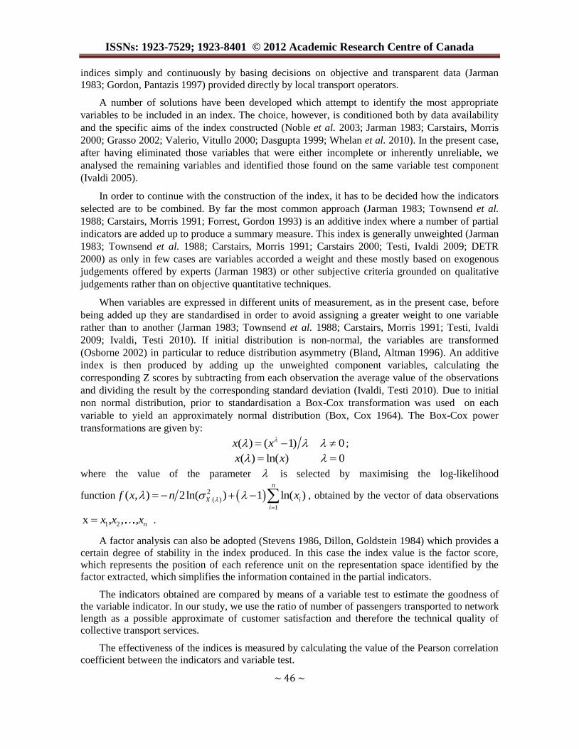
transformations are given by:

( ) ( 1)x x 0 ;

( ) ln( )x x 0

where the value of the parameter is selected by maximising the log-likelihood

function 2

( )

1

( , ) 2ln( ) 1 ln( )n

X i

i

f x n x

, obtained by the vector of data observations

1 2x , , , nx x x .

A factor analysis can also be adopted (Stevens 1986, Dillon, Goldstein 1984) which provides a

certain degree of stability in the index produced. In this case the index value is the factor score,

which represents the position of each reference unit on the representation space identified by the

factor extracted, which simplifies the information contained in the partial indicators.

The indicators obtained are compared by means of a variable test to estimate the goodness of

the variable indicator. In our study, we use the ratio of number of passengers transported to network

length as a possible approximate of customer satisfaction and therefore the technical quality of

collective transport services.

The effectiveness of the indices is measured by calculating the value of the Pearson correlation

coefficient between the indicators and variable test.

Review of Economics & Finance

~ 47 ~

As regards the division of the cities under examination into groups, homogenous groupings can

be used (Carstairs 2000). In order to identify classes and discriminate amongst different levels of

inequality, the literature suggests either breaking down the distribution of indices on the basis of

parameters (Carstairs et al. 1991), or alternatively using population deciles (Jarman 1984;

Townsend et al. 1988; Cadum et al.1999). When a comparison between different index types is

required, as in the present case, a parameter-based approach that maintains the discriminatory

characteristics of distribution is recommended (Carstairs 2000).

Therefore, index distribution was divided into three classes, with class 1 identifying the cities

with the highest indicator.

3. Results

A total of 29 variables emerged, although some of these were excluded due to a lack of data

(e.g. punctuality/delays, vehicle saturation, off-peak frequency). The following 16 variables were

inserted in the initial factor analysis: average number of employees/network length; average number

of vehicles in service/network length; vehicle-km produced; number of vehicles registered in the

past 5 years/network length; average commercial speed; protected (e.g. bus lanes) network

length/network length; total personnel costs/network length; total fuel costs/network length; total

raw material and maintenance costs/network length; peak service frequency (in minutes); hourly

standard fare rate; number of place-km produced; number of passenger information panels per

stop/total number of stops; cost of monthly season ticket; number of stops/network length; average

fleet age.

To reduce distortions deriving from the differences in network sizes, size-related variables were

compared to network length before carrying out an analysis of the principal components.

Subsequent extraction and rotation algorithm tests revealed stability of the components extracted as

well as the particular effectiveness of the Varimax rotation method (Kaiser 1958).

The exploratory factor analysis produced 4 variables placed on the first factor in addition to the

test variable: vehicle-km produced; number of vehicles registered in the past 5 years/network

length; average number of employees/network length; average number of vehicles in service/

network length (table 2).

These are movement-related variables2. It may said that service quality levels derive from

service quantity in that these variables are indirectly linked to network capillarity and journey times.

These variables are, however, less subject to subjectivity on the part of questionnaire respondents

and therefore correctly placed in the first factor. Variables referring to speed and frequency are

inevitably more difficult to be collected by transport operators in an objective and symmetric way,

which in turn makes inter-firm comparisons difficult. However, data relating to vehicles km,

number of vehicles registered in the last five years, average number of employees, average number

of vehicles in service are less exposed to respondent subjectivity. Needless to say, data supplied by

operators is regarded as “true and fair” and not intentionally false or misleading (alas, in some cases

we were forced to eliminate a variable from our analysis when it was clear that data supplied was

not reliable). Surprisingly, the variable “places km produced” appears in the fourth factor rather

than in the first as predicted.

Three of the five variables placed in the second factor (total personnel costs/network length;

total fuel costs/network length; raw material and maintenance costs/network length) are clearly

linked, being fundamental business cost related data. They are consequently correctly correlated

with each other and equally correctly not placed on the first factor as this is the factor most

2 With the exception of the variable ‘places km produced’, which is placed in the fourth factor.

ISSNs: 1923-7529; 1923-8401 © 2012 Academic Research Centre of Canada

~ 48 ~

representative of technical quality. In this case we can see how, having inserted also business cost

related data, such data are correctly correlated with each other but, being placed on a factor different

from the first, they are not representative of technical quality.

Table 2. Exploratory factor analysis - Rotated Component Matrix(a)

Components

Items 1 2 3 4

Vehicles km produced 0.859 -0.202 0.006 0.101

Number of vehicles registered in last 5

years/network length

0.819 -0.178 0.079 -0.052

Number of passengers carried/network length

VARIABLE TEST

0.816 -0.255 0.404 -0.053

Average number of employees/network length 0.684 -0.232 0.613 0.117

Number of vehicles in service/network length 0.677 -0.203 0.628 0.163

Total personnel costs/network length -0.123 0.918 -0.295 -0.147

Total fuel costs/network length -0.146 0.905 -0.314 -0.163

Raw material and maintenance costs/network length -0.183 0.869 -0.326 -0.164

Peak service frequency (minutes) -0.280 0.721 0.511 -0.053

Hourly standard fare 0.242 -0.612 0.096 -0.213

Number of stops/network length 0.175 -0.168 0.795 -0.022

Monthly season ticket (in Euros) -0.079 -0.285 0.747 0.215

Length of protected network (in km)/network length 0.367 -0.163 0.696 0.251

Average commercial speed (in km/h) -0.476 0.124 -0.618 -0.126

Number of places km produced 0.055 -0.143 -0.012 0.909

Number of passenger information panels at stops/

number of stops

0.096 0.004 0.256 0.857

Average fleet age 0.341 0.022 -0.302 -0.365

Notes: Extraction Method: Principal Component Analysis.

Rotation Method: Varimax with Kaiser Normalization. - a Rotation converged in 7 iterations.

The variables expressed in the third factor are number of stops/network length; cost of monthly

season ticket; protected network length/network length; average commercial speed, whilst those in

the fourth factor are number of place-km produced; number of passenger information panels per

stop/total number of stops; average fleet age. Despite being closely linked to the technical

effectiveness of the service offered, these variables do not appear in the first factor owing to the

higher degree of subjectivity in the answers. In order to discover the reasons for this, interviews and

in some cases visits to the operators in question were carried out, which revealed that the methods

of extracting data varied from operator to operator. As a result, comparison between variables was

not possible. The principal differences in data extraction amongst operators regarded: commercial

speed; the role and measurement of passenger information systems at stops, which in some cases

included those either no longer activated or currently under construction; the role and measurement

of the protected network, which in some cases included the entire transport network in kilometers

instead of the distance in kilometers effectively protected, e.g. bus lanes.

Priority in the choice of variables to be used in the indicator should be given to those that

appear in the first component and which have a positive value (Ivaldi 2005). It should be observed

how these four variables represent those with reduced subjective content and which therefore have

the greatest degree of homogeneousness with each other from operator to operator.

Review of Economics & Finance

~ 49 ~

Table 3. Index of inequality in local public transport

The index therefore is made up of the

following variables: vehicle km produced; number

of vehicles registered in the last five years/network

length; average number of employees/network

length; number of vehicles in service/network

length. The index was calculated firstly by using an

additive measure that added the variables up. As we

have seen, owing to the lack of homogeneousness in

the way the variables are measured, the variables

were standardized. The z-score for each variable

was therefore calculated, obtained by subtracting

from each observation the average value of

distribution and dividing the result by its standard

deviation. The overall index is made up as a result

by the sum of the four unweighted z-scores.

Table 3 illustrates the index of inequality in

local public transport for each regional centre.

The index has a zero average and standard

deviation of 4.19; this value is due to correlation

amongst the variables making up the index. As

expected, the distribution of the indicator is not

perfectly normal with a degree of positive

asymmetry (Pearson’s asymmetry index: 0.92).

By using a factor analysis of the variables

previously extracted, it is possible to have an alternative measure of comparison with the additive

index that produces as an index of inequality the factor score, which represents the position of each

regional capital in the space of representation identified by the factor extracted, which in turn

synthesises information taken from the partial indicators (Ivaldi 2005; Michelozzi et al. 1999). This

indicator shows positive asymmetry (Pearson’s asymmetry index: 0.76, zero average and a standard

deviation of 0.97.

The index constructed using a factor analysis confirmed the findings produced by the additive

measure. Sensitivity analysis reveals that the two methods used in variable selection and index

construction produce practically identical results. An indication of this is how factor index and

additive index ranks coincide, with the Spearman test producing a correlation coefficient of value 1.

Indicator validation however is required. The measure chosen to do this was that provided by the

variable “number of passengers transported/network length”. Both indicators recorded a Pearson

value of 91%. In both cases, the indicator proposed presents therefore a high degree of correlation

(near the maximum value it can have) with the measure of service use.

In table 4 and figure 1, the regional capitals are grouped into 3 homogeneous classes on the

basis of the standard deviation of the distribution of the indicator. To identify three homogeneous

categories, the value +2/3 was used as cut off. The analysis was carried out using the additive

index but similar results are obtained, albeit with fewer extreme classes, using a factor index.

The classes identify different levels of technical quality which, in turn, distinguish three

classes, with class 1 identifying the cities with the highest service levels.

City Additive

index

Factor

index

Milan 9.96 2.25

Rome 6.57 1.52

Naples 5.49 1.38

Palermo 4.59 1.10

Bologna 4.12 0.93

Turin 2.29 0.53

Verona -0.17 0.01

Genoa -0.42 -0.10

Trieste -0.47 -0.11

Florence -1.17 -0.28

Ancona -1.63 -0.37

Cagliari -2.42 -0.56

Bari -2.84 -0.66

Trento -2.92 -0.69

Reggio Calabria -3.88 -0.92

L'aquila -4.04 -0.94

Aosta -4.14 -0.97

Perugia -4.32 -1.02

Campobasso -4.61 -1.08

ISSNs: 1923-7529; 1923-8401 © 2012 Academic Research Centre of Canada

~ 50 ~

Figure 1. Map showing the index division of inequality in the provision of local public transport

Table 4. Index division of inequality in the provision of local public transport

Index class City

Class 1 Milan, Rome, Naples, Palermo, Bologna

Class 2 Turin, Verona, Genoa, Trieste, Florence, Ancona, Cagliari

Class 3 Trento, Bari, Reggio Calabria, L’Aquila, Aosta, Perugia, Campobasso

Review of Economics & Finance

~ 51 ~

4. Discussion and Conclusions

On the basis of the analysis carried out, three inter-related aspects emerge: (1) the performance

of what we refer to as the “technical” quality of local public transport in Italy; (2) the extent and

quality of political awareness regarding collective urban transport and its impact on service quality;

(3) the Italian legislative context in which the local public transport sector operates.

1. As regards performance in technical quality, the analysis of Italian regional centres reveals

different levels of service, and places only five cities in band 1, with seven cities both in band 2 and

band 3. In particular, Rome, Naples, Palermo and Bologna recorded the highest levels in the

effectiveness (technical as opposed to perceived) of the service provided. In intermediate band 2,

seven cities record service levels inferior to those of the top five: Turin, Genoa, Florence, Verona.

Trieste. Cagliari and Ancona. The poorest performing cities measured on the basis of the indicators

selected are positioned in band 3: Reggio Calabria, Perugia, Trento, L’Aquila, Campobasso and

Aosta.

Geographically, no qualitative differences emerge between the north and south of Italy, the

latter generally viewed as the economically most problematical area of the country. In fact, both

areas have cities placed in the first and third classes. Instead, size in terms of number of inhabitants

and area (km2) appears to be of greater significance. In fact, with some exceptions, the largest cities

are those with the highest qualitative performances, confirming the fact that where consolidated

policies in support of local public transport are in place allied to restrictions on the use of private

cars, service levels improve3 (Canali et al. 2000). A vicious cycle of congestion that negatively

impacts collective transport is more likely in cities with no effective urban mobility policy: the

greater the use of the motor car, initially justified by the inherent characteristics of this form of

transport – comfort, flexibility, capillarity, speed – determines a fall in the demand for public

transport, a reduction in service and a subsequent worsening of quality (both measurable and

perceived), which leads to a further fall in market share. Such a vicious cycle is accentuated by the

fact that increased levels of private transport create greater congestion which proportionally has a

more damaging effect on public transport4 (Musso, Burlando 1999), unless equipped with suitable

infrastructure to contrast the impact of private transport. In brief, medium-sized cities, where there

3 A study carried in 2000 investigating the relationship between government (central and local) mobility

policies and the size of urban areas reveals significant differences in the number of policies applied in large cities and medium-sized centres. In particular, the analysis concluded that the quantity and quality of mobility-related measures applied in large cities is markedly greater than in smaller ones. In fact, larger cities have a range of policies that are in general more innovative and which are applied synergically. For more details, see Canali, Musso, Burlando, Pelizzoni (2000).

4 Congestion negatively affects collective transport more than private transport owing to (i)itinerary

rigidities that prevent route optimisation on the basis of traffic conditions; (ii) waiting times at stops,

which being a function of the ratio between the average space occurring between two successive

vehicles and their speed, will clearly increase with a decrease in vehicle speeds; (iii) delays in

timetabled services and subsequent reductions in the reliability and quality of the service offered.

The result is that congestion, normally caused by private transport, penalises individual transport to a

lesser extent in comparison to collective transport, which in turn acts as further incentive to use

private forms of transport. The effect of this is a reduction in local public transport revenues against a

backdrop of rising costs due to increased fuel consumption and above all longer driving times for the

same route. The effect for the transport operator is a reduced capacity to cover running costs through

service-generated revenues; a reduction in the effectiveness of the service offered also negatively

impacts business management efficiency. See Musso, Burlando (1999) chapter 9.

ISSNs: 1923-7529; 1923-8401 © 2012 Academic Research Centre of Canada

~ 52 ~

are proportionally fewer problems of movement from one place to another and where private

transport is the primary mobility solution5, pay a high price for the limited attention given to public

transport in the form of lower technical quality levels. In large cities, where congestion, pollution

and negative externalities are urgent issues, local government has long given priority to the

development of effective strategies for the organisation of mobility. Local public transport in Italy’s

largest cities in fact has a higher level of technical quality due to, on one hand, greater attention on

the part of local government and the subsequent application of a set of mobility-dedicated measures

and, on the other, proportionally less dependence on private transport, which alleviates the vicious

cycle described above.

2. An aspect related to public transport performance is the importance given to the question of

urban collective mobility by local government. Our analysis of the Italian context reveals overall

similarities in funding levels across regional centres. Lower levels of technical quality coincide with

municipalities where less is spent on local public transport. It is likely therefore that low technical

quality levels stem from, in addition to managerial incapacity, scarce attention to the problem and

limited implementation of measures aimed at raising public transport performance. Such measures

have been widely discussed in the literature and can be summarised as follows6:

- separation of collective transport from private transport and restrictions on the latter in order

to break the vicious cycle whereby an increase in private transport determines a worsening in the

qualitative level of local public transport;

- increase of intermodality aimed at favouring positive interdependencies between private and

public transport;

- infrastructure policies (local public transport dedicated infrastructures including low cost

initiatives such as traffic separators for bus lanes);

- innovation in vehicles, services, information technologies, payment systems;

- quality monitoring and control.

Increased political focus on the issue of urban mobility will have a positive effect on local

public transport in terms of performance: greater attention to collective transport will create an

awareness of the need for a synergic approach in applying the measures outlined above which will

in turn shift the emphasis onto government (central and local) rather then the local transport

operator as the key player in governing the complex systems of both public and private mobility.

With this in mind, greater collaboration is required between government (ultimately responsible for

policy decisions in the area of urban mobility) and transport operators, particularly in those cities

with the lowest levels of technical quality.

3. A further key element is the legislative setting in which Italian local public transport operates

and in particular the current state of reforms started more than 15 years ago. For decades local

public transport in Italy has suffered from financial unsustainability allied to an inability to address

and respond in quantitative and qualitative terms to the needs of the mobility demand side. The

application, albeit belated, of the underlying principles contained in Legislative decree 422/1997

would go some way towards containing (as well as other things) service ineffectiveness. A case in

point is the fact that a conduit for improvements is the elimination foreseen by the reform of a

5 Reference is made here to motorised transport and not to alternatives such as travelling by bicycle or

on foot which, due to shorter average distances, may be an attractive alternative. It should be noted, however, that these forms of transport are less feasible in urban areas where the average age of the population is high. In this case, public transport is the more convenient form of transport.

6 For details regarding the measures, see Musso, Burlando (1999), chapter 8.

Review of Economics & Finance

~ 53 ~

protectionist system that effectively prevented transport operators from failing. Legislative decree

422/1997 outlined an extremely innovative institutional and management framework that

represented a significant break with the past. Its main features were:

- the transfer of legislative responsibility from central government to regional and local levels.

By bringing decision making closer to transport users, the services provided should respond more

effectively to the mobility needs of the local community;

- the introduction of tender procedures that sought to discourage the concession of transport

services by local government to firms controlled by local government itself. Such practices create

monopolistic conditions in which the transport operator, being exempt from market discipline, i.e.

the risk of failure, has little incentive to seek operational efficiency.

The overriding aim of the Decree was to reduce the sector’s inefficiency and ineffectiveness.

However, the liberalisation of local public transport, which has been the subject of heated debate for

over 15 years, has yet to come about. Clear, definitive and binding legislation is required in order to

bring order to a sector in serious difficulty. The aspects identified at points 2 and 3 above show that

the causes for the failure of so many major Italian cities to reach the top performance band (band 1)

do not lie exclusively with transport operators. In fact, these cities’ poor performance levels can be

cogently attributed also to the absence of a coherent approach to mobility at local government level

plus a legislative scenario characterised by a plethora of ill-conceived and often contradictory

measures.

What emerges from the present work is the need for the periodic production of business data by

transport operators to be used in the construction of performance indices. Consistent with the role of

planning and control envisaged by the reforms mentioned above, government should determine a

method of data collection and index construction that is uniform for all operators.

Homogeneousness in these areas will allow for an efficient analysis of transport operators’

performances rather than analytical inefficiencies inherent in the present situation. In fact, the

marked differences in data collection methodologies lead to scarce comparability of data and

excessive collection costs (initial analyses often have to be integrated by interviews regarding single

items of data). Without the changes outlined here, a reduction in inequality in local transport

services in Italy is not on the immediate horizon.

Although if it is extremely difficult to obtain homogeneous data, future work may lead to use

this method for the analysis of the LPT sector in other countries allowing therefore, to carry on

comparisons between different cities in different countries.

References

[1] Benach J., Yasui Y. (1999), “Geographical patterns of excess mortality in Spain explained by two

indices of deprivation”, Journal of Epidemiology and Community Health, 53(7):423-431.

[2] Bland J., Altman D. (1996), “Statistics Notes: Transforming data”, British Medical Journal, 312:

770.

[3] Box G., Cox D. (1964), “An analysis of transformations (with discussion)”, Journal of the Royal Statistical Society, Series B(Methodological), 26(2): 211-252.

[4] Cadum E., Costa F., Biggeri A., Martuzzi M. (1999), “Deprivazione e mortalità: un indice di

deprivazione per l’analisi delle disuguaglianze su base geografica”, Epidemiologia e Prevenzione,

23: 175-187.

[5] Canali C., Musso E., Burlando C., Pelizzoni C. (2000), “Policies for sustainable mobility in Italian

cities”, In: Urban Transport VI, Wessex Institute of Technology (Wit Press), Southampton, Boston.

[6] Carstairs V. (2000), “Socio-economic factors at area level and their relationship with health”, In:

Elliott P., Wakefield J., Best N., and Briggs D. (Eds.), Spatial Epidemiology Methods and Applications (pp. 51-68). Oxford University Press.

ISSNs: 1923-7529; 1923-8401 © 2012 Academic Research Centre of Canada

~ 54 ~

[7] Carstairs V., Morris R. (1991), Deprivation and Health in Scotland, Aberdeen University Press.

[8] Dasgupta P. (1999), Valuation and Evaluation: Measuring the Quality of Life and Evaluation

Policy, University of Cambridge and Beijer International Institute for Ecological Economics.

Stockholm.

[9] Department of Environment Transport and the Regions (DETR) (2000), “Indices of Deprivation

2000”, Regeneration Research Summary, No.31: 3-42.

[10] Dillon W., Goldstein M. (1984), Multivariate Analysis Method and Application, Wiley

[11] Forrest R., Gordon D. (1993), People and Places: a 1991 Census atlas of England, SAUS

University of Bristol.

[12] Gordon D., Pantazis C. (1997), Breadline Britain in the 1990s, Ashgate Publishing Limited.

England.

[13] Grasso M. (2002), “Una misurazione del benessere nelle regioni italiane”, Politica Economica,

18(2): 261-292.

[14] Hales S., Black W., Skelly C., Salmond C., Weinstein P. (2003), “Social deprivation and the public

health risks of community drinking water supplies in New Zealand”, Journal of Epidemiology and

Community Health, 57: 581-583.

[15] Ivaldi E. (2005), Indicatori di deprivazione come misura di svantaggio sociale: il caso dell’area metropolitana genovese, Tesi di dottorato. Università degli Studi di Genova.

[16] Ivaldi E., Testi A. (2010), Genoa Index of Deprivation (GDI): An Index of Material Deprivation for

Geographical Areas. Social Indicators: Statistics. Trends and Policy Development Eds Candace M.

Baird. Nova Publisher ISBN: 978-1-61122-841-0 pp:75-97.

[17] Jarman B. (1983), “Identification of underprivileged areas”, British Medical Journal, 286: 1705-09.

[18] Jarman B. (1984), “Underprivileged areas: validation and distribution of scores”, British Medical

Journal, 289: 1587-1592.

[19] Kaiser H.F. (1958), “The varimax criterion for analytic rotation in factor analysis”, Psychometrika

23: 187–200.

[20] Michelozzi P., Perucci C., Forastiere F., Fusco D., Ancona A., Dell’orco V. (1999), “Differenze

sociali nella mortalità a Roma negli anni 1990-1995”, Epidemiologia e Prevenzione, 23: 230-238.

[21] Noble M., Smith G., Wright G., Dibben C., Lloyd M, Ratcliffe A., McLellan D., Sigala M. Anttila

C. (2003), Scottish Indices of Deprivation 2003, Scottish Executive, Edinburgh.

[22] Osborne J. (2002), “Notes on the use of data transformations, Practical Assessment”, Research and

Evaluation, 8(6): 912-935.

[23] Stevens J. (1986), Applied Multivariate Statistics for the Social Sciences, Hillsdale.

[24] Testi A., Ivaldi E., Busi A. (2005), Caratteristiche e potenzialità informative degli indici di

deprivazione . Tendenze nuove 2/2005.

[25] Testi A., Ivaldi E. (2009), “Material versus social deprivation and health: a case study of an urban

area”, The European Journal of Health Economics, 10(3): 323-328.

[26] Testi A., Ivaldi E. (2011), “Measuring Progress in Health through Deprivation Indexes”, Review of Economics & Finance, 11(2): 49-57.

[27] Townsend P. (1987), “Deprivation”, Journal of Social Policy, 16(2): 125-146.

[28] Townsend P., Phillimore P., Beattie A. (1988), Health and Deprivation: Inequality and the North,

London: Croom Helm.

[29] Valerio M., Vitullo F. (2000), “Sperimentazione di un indice di svantaggio sociale in Basilicata”,

Epid Prev 2000, 24: 219-223.

[30] Whelan C.T., Lucchini M., Pisati M., Maître B. (2010), “Understanding the socio-economic

distribution of multiple deprivation: An application of self-organising maps”, Research in Social Stratification and Mobility, 28(3): 325-342.