an innovative solution to nasa’s neo impact threat
TRANSCRIPT

Final Technical Report of a NIAC Phase 2 Study December 9 2014
NASA Grant and Cooperative Agreement Number NNX12AQ60G
NIAC Phase 2 Study Period 09102012 ndash 09092014
An Innovative Solution to NASArsquos NEO ImpactThreat Mitigation Grand Challenge and FlightValidation Mission Architecture Development
PI Dr Bong Wie Vance Coffman Endowed Chair Professor
Asteroid Deflection Research Center
Department of Aerospace Engineering
Iowa State University Ames IA 50011
email bongwieiastateedu
(515) 294-3124
Co-I Brent Barbee Flight Dynamics Engineer
Navigation and Mission Design Branch (Code 595)
NASA Goddard Space Flight Center
Greenbelt MD 20771
email brentwbarbeenasagov
(301) 286-1837
Graduate Research Assistants Alan Pitz (MS 2012) Brian Kaplinger (PhD 2013)
Matt Hawkins (PhD 2013) Tim Winkler (MS 2013) Pavithra Premaratne (MS 2014)
Sam Wagner (PhD 2014) George Vardaxis Joshua Lyzhoft and Ben Zimmerman
NIAC Program Executive Dr John (Jay) Falker
NIAC Program Manager Jason Derleth
NIAC Senior Science Advisor Dr Ronald Turner
NIAC Strategic Partnerships Manager Katherine Reilly
Contents
1 Hypervelocity Asteroid Intercept Vehicle (HAIV) Mission Concept 2
11 Introduction 2
12 Overview of the HAIV Mission Concept 6
13 Enabling Space Technologies for the HAIV Mission 12
131 Two-Body HAIV Configuration Design Tradeoffs 12
132 Terminal Guidance SensorsAlgorithms 13
133 Thermal Protection and Shield Issues 14
134 Nuclear Fuzing Mechanisms 15
2 Planetary Defense Flight Validation (PDFV) Mission Design 17
21 The Need for a PDFV Mission 17
22 Preliminary PDFV Mission Design by the MDL of NASA GSFC 20
221 Overview 20
222 HAIV System and Mission Design 20
223 Terminal Guidance Navigation and Control Subsystem 26
224 Future Work for HAIV Mission Design 29
225 Summary 31
23 Target Selection for the PDFV Mission 31
231 Reference Targets of the Don Quijote Mission Study 32
232 Target Selection Problem Formulation 32
233 Direct Intercept PDFV Mission 35
24 Recommendations for Planetary Defense 38
3 Terminal Intercept Guidance with Optical and Infrared Seekers 43
31 Introduction 43
32 Optical Image Rendering 49
321 3D Polyhedron Optical Model for an Irregularly Shaped Asteroid 49
i
322 Camera Focal Plane 50
323 Lighting Conditions 52
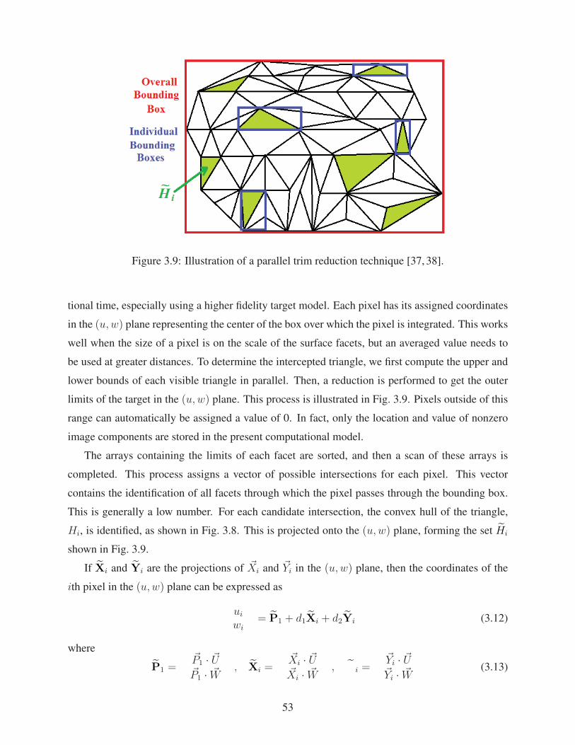
324 Pixel Value Assignment 52
325 Line-of-Sight Vector 54
33 Terminal Intercept Guidance with Optical Cameras 54
34 IR TelescopeSeeker Characterization 55
341 IR TelescopeSeeker 55
342 Classical Cassegrain Telescope Optics 55
343 Signal-to-Noise Ratio 61
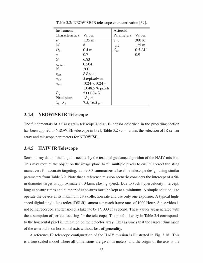
344 NEOWISE IR Telescope 65
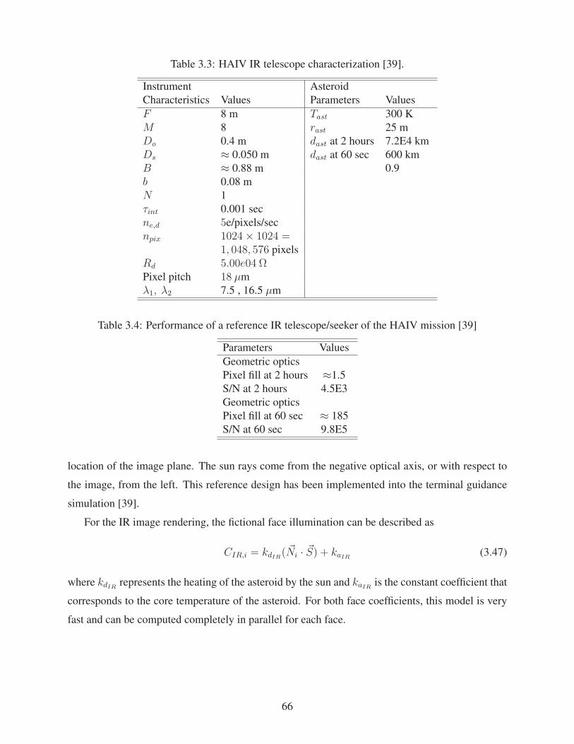
345 HAIV IR Telescope 65
35 Terminal Intercept Guidance with an IR Seeker 67
4 Hypervelocity Kinetic Impact and Nuclear Subsurface Explosion Modeling and Simshy
ulation 70
41 Introduction 70
42 GPU-based ASPH Hydrocode Development 71
421 Adaptive Smoothed Particle Hydrodynamics (ASPH) Method 72
422 Tensor Damage Model 74
423 Neighbor Finding Implementation 75
424 Grid Generation 75
43 Energy-Coupling Models 77
431 Introduction 77
432 Energy Deposition Modeling 78
433 Tillotson Equation of State 80
434 Shock Equation of State 82
435 Jones-Wilkins-Lee (JWL) Equation of State 82
44 GPU-based ASPH Hydrocode Simulations 82
441 Disruption of an Asymmetric Asteroid Model 84
442 Subsurface Explosion Sensitivity Analysis 86
443 GPU-Accelerated Computations 89
45 Thermal Shield Analysis and Design 91
451 Thermal Analysis Procedure 91
452 Improved Thermal Analysis Procedure 97
46 Whipple Shield Analysis and Design 98
ii
5 Suborbital Intercept and Disruption of NEOs 108
51 Introduction 108
52 An Optimum Suborbital Intercept Problem and Its Solutions 111
521 Problem Formulation 111
522 Intercept Trajectory Optimization 115
523 Suborbital Intercept Examples 115
524 Late Intercept Solutions 118
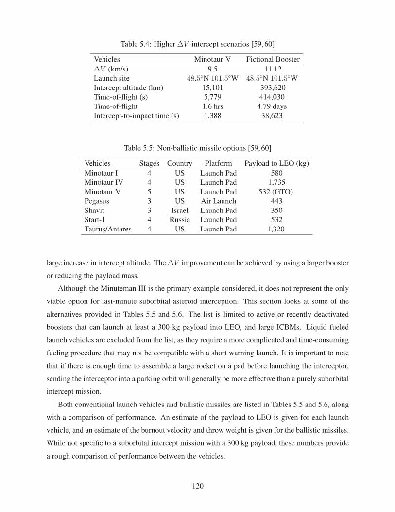
53 Higher ΔV Interceptors 119
54 Practical Issues and Future Research Work 121
541 Fragmentation and Airbursts 121
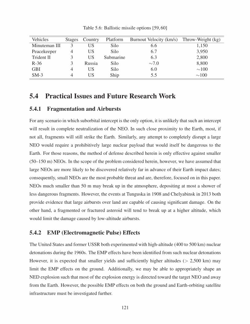
542 EMP (Electromagnetic Pulse) Effects 121
543 Launch Vehicle Mission Planning Issues 122
544 Future Research Work 122
55 ATLAS (Asteroid Terrestrial-impact Last Alert System) 123
6 Close Proximity Dynamics and Control Around Asteroids 125
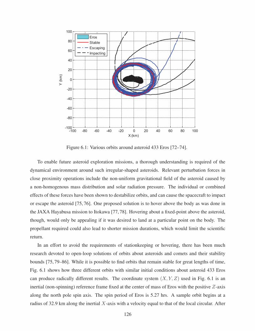
61 Introduction 125
62 Gravitational Models of an Irregular-Shaped Asteroid 128
621 Spacecraftrsquos Equation of Motion 128
622 Polyhedron Gravitational Model 128
623 Spherical Harmonics Expansion Model 131
624 Inertia Dyadic Gravitational Model 133
625 Comparison of Gravitational Models 137
63 Close Proximity Dynamics and Fuel-Efficient Orbit Control 138
631 Close Proximity Orbital Dynamics 138
632 Fuel-Efficient Close Proximity Orbit Control 140
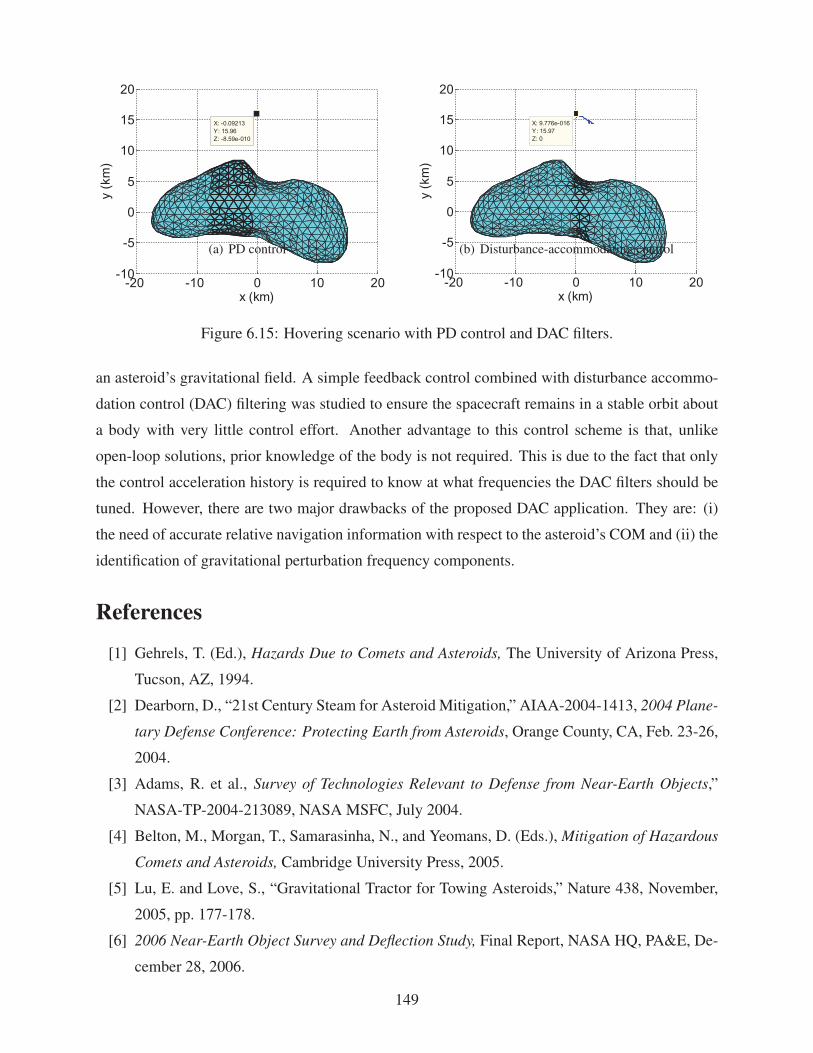
64 Summary 148
iii
List of Figures
11 A summary of the ideal deflection ΔV performance characteristics of nuclear
standoff explosions [9] 4
12 Initial conceptual illustration of a two-body hypervelocity asteroid intercept vehishy
cle (HAIV) system which was proposed for a NIAC Phase 1 Study in 2011 [12] 6
13 A notional depiction of the HAIV mission concept further investigated for a NIAC
Phase 2 Study in 2012ndash2014 7
14 HAIV configuration options [13] 7
15 A reference HAIV flight system and its terminal guidance operational concept [13] 8
16 A 70-m asymmetric asteroid model disrupted by a 10-kms kinetic impact and a
subsequent 70-kt nuclear subsurface explosion of the HAIV system [17ndash19] 10
17 Illustration of the disruption modeling and simulation problem [23] 10
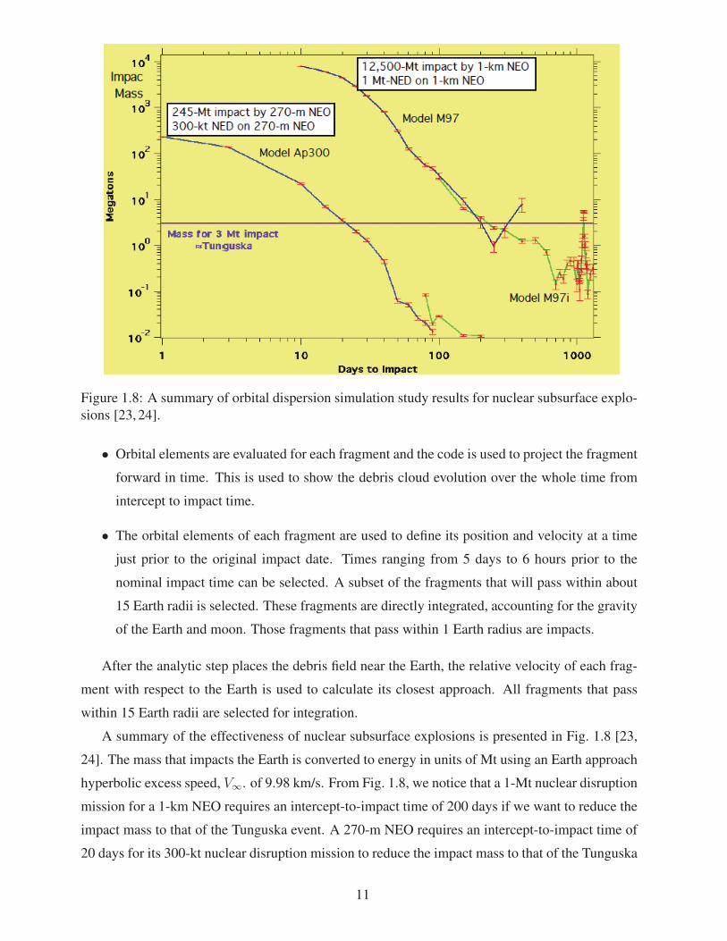
18 A summary of orbital dispersion simulation study results for nuclear subsurface
explosions [23 24] 11
21 The Deep Impact mission trajectory [25ndash27] 18
22 An experimental HAIV flight system designed by the MDL of NASA GSFC [15] 21
23 A reference HAIV launch configuration with Atlas V 401 [15] 22
24 A reference PDFV mission trajectory for a target asteroid (2006 CL9) [15] 24
25 HAIV flight validation mission timeline by the MDL of NASA GSFC [15] 25
26 Block diagram of the Autonomous Navigation System (ANS) of an experimental
HAIV [15] 27
27 Block diagram of the Attitude Control System (ACS) of an experimental HAIV [15] 28
28 Monte Carlo simulation results for intercepting an ideal 100-m target asteroid using
the B-plane targeting method [15] 29
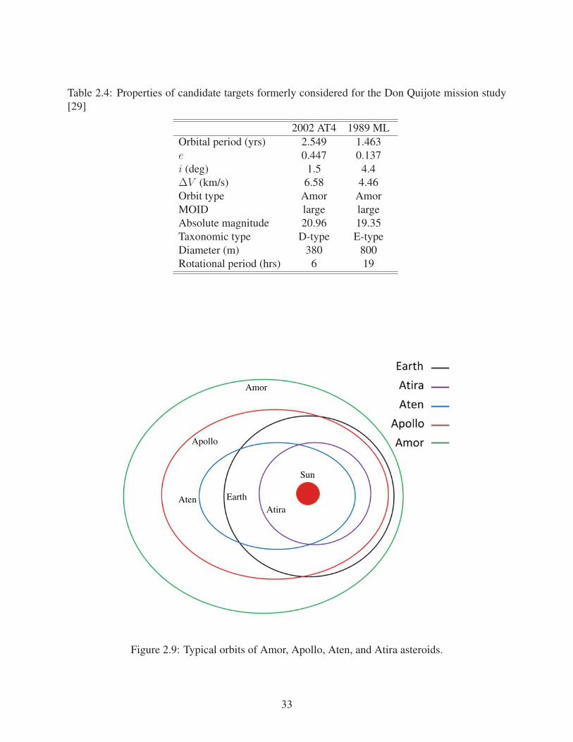
29 Typical orbits of Amor Apollo Aten and Atira asteroids 33
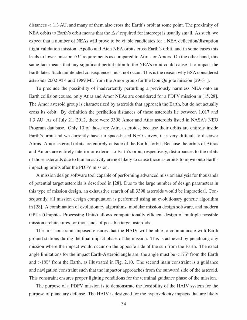
210 Illustration of the Earth-Sun-Asteroid line-of-sight communication angle excluded
for the PDFV mission [28] 35
iv
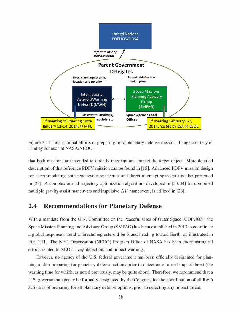
211 International efforts in preparing for a planetary defense mission Image courtesy
of Lindley Johnson at NASANEOO 38
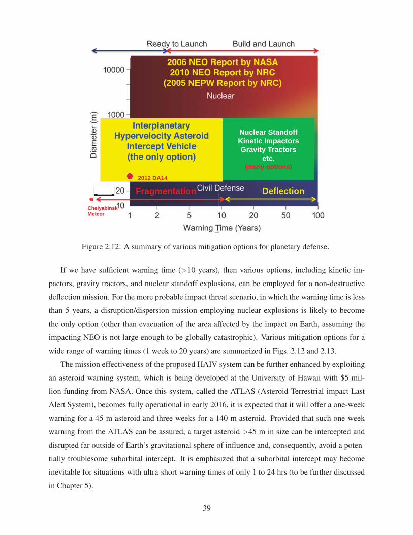
212 A summary of various mitigation options for planetary defense 39
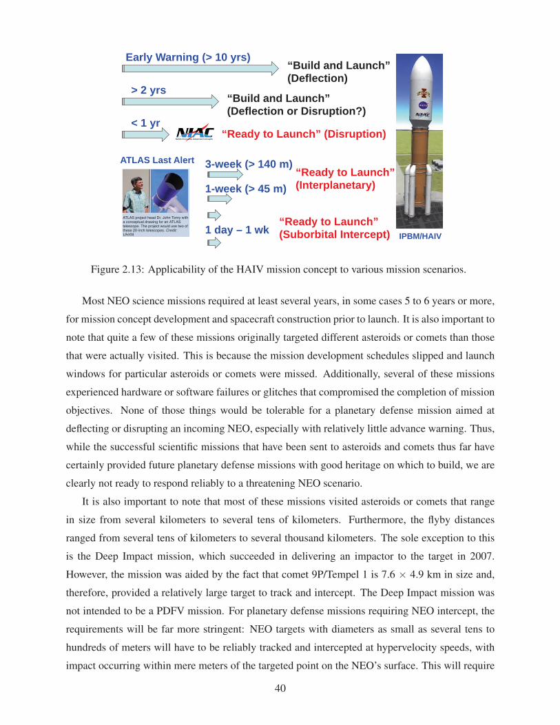
213 Applicability of the HAIV mission concept to various mission scenarios 40
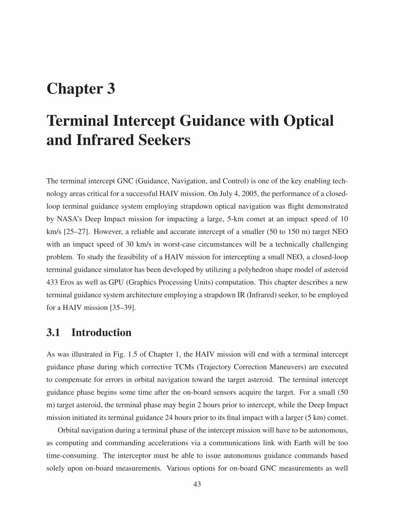
31 Two-dimensional geometry illustration of the terminal intercept guidance problem
[35 36] 44
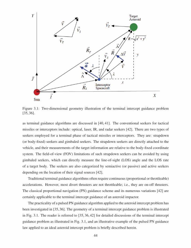
32 Trajectories line-of-sight angle commanded acceleration and applied accelerashy
tion of the pulsed PN guidance law applied to an ideal asteroid intercept probshy
lem [35 36] 46
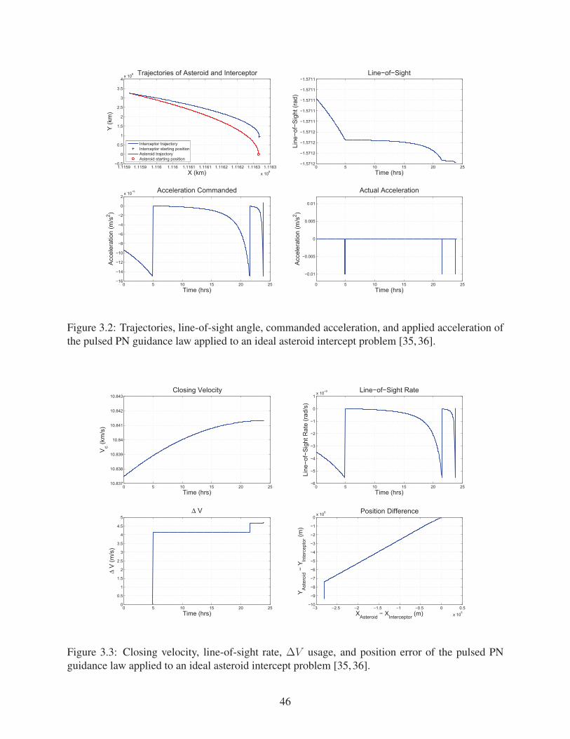
33 Closing velocity line-of-sight rate ΔV usage and position error of the pulsed PN
guidance law applied to an ideal asteroid intercept problem [35 36] 46
34 A 3D model of asteroid 433 Eros generated using NEARrsquos laser rangefinder meashy
surements (left) and the surface gravitational acceleration of Eros computed using
its polyhedron shape model (right) [37] 47
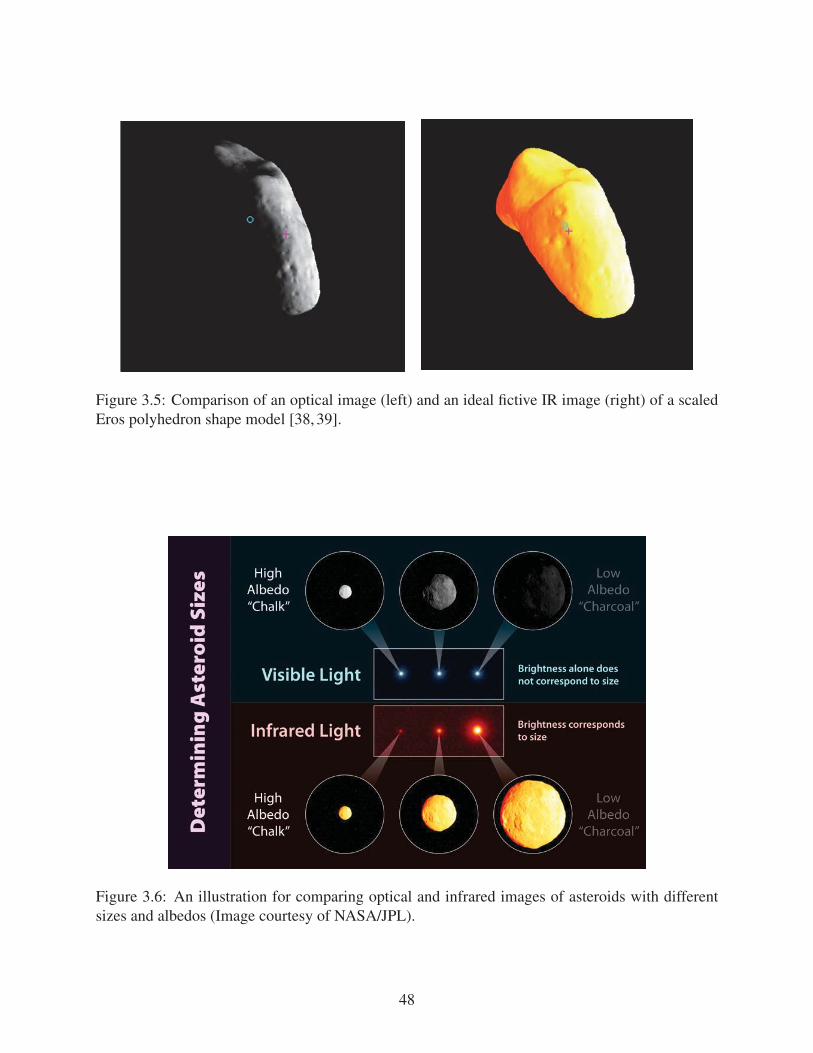
35 Comparison of an optical image (left) and an ideal fictive IR image (right) of a
scaled Eros polyhedron shape model [38 39] 48
36 An illustration for comparing optical and infrared images of asteroids with differshy
ent sizes and albedos (Image courtesy of NASAJPL) 48
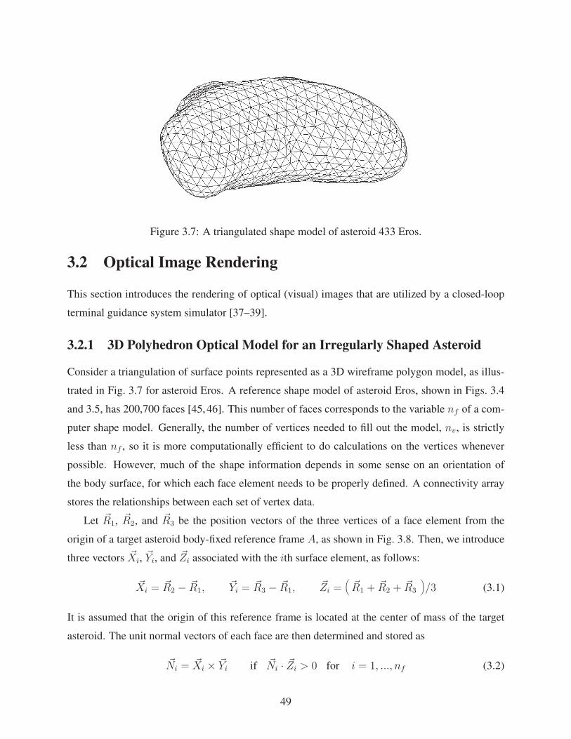
37 A triangulated shape model of asteroid 433 Eros 49
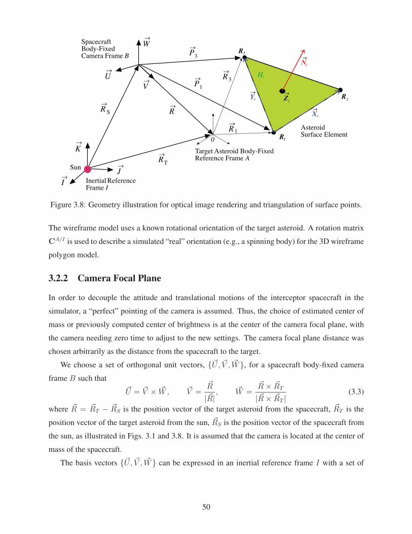
38 Geometry illustration for optical image rendering and triangulation of surface points 50
39 Illustration of a parallel trim reduction technique [37 38] 53
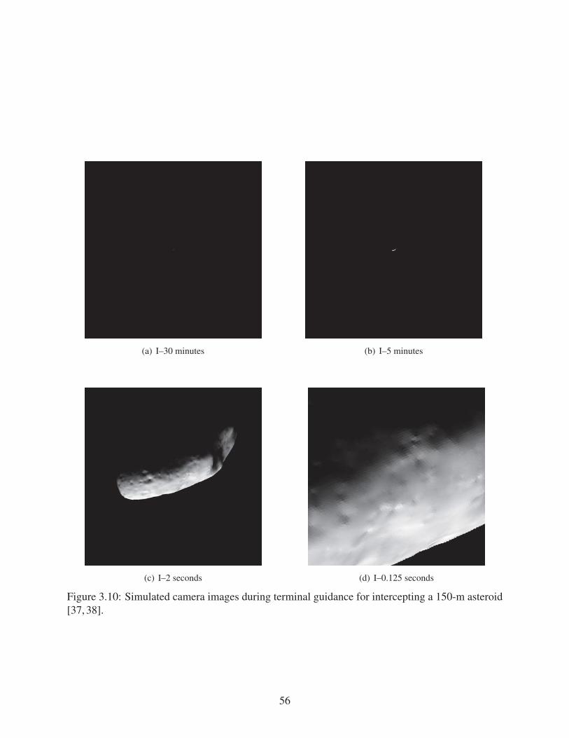
310 Simulated camera images during terminal guidance for intercepting a 150-m astershy
oid [37 38] 56
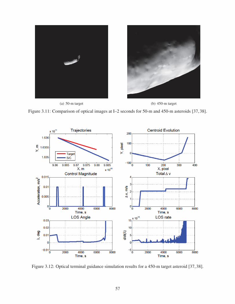
311 Comparison of optical images at Indash2 seconds for 50-m and 450-m asteroids [37 38] 57
312 Optical terminal guidance simulation results for a 450-m target asteroid [37 38] 57
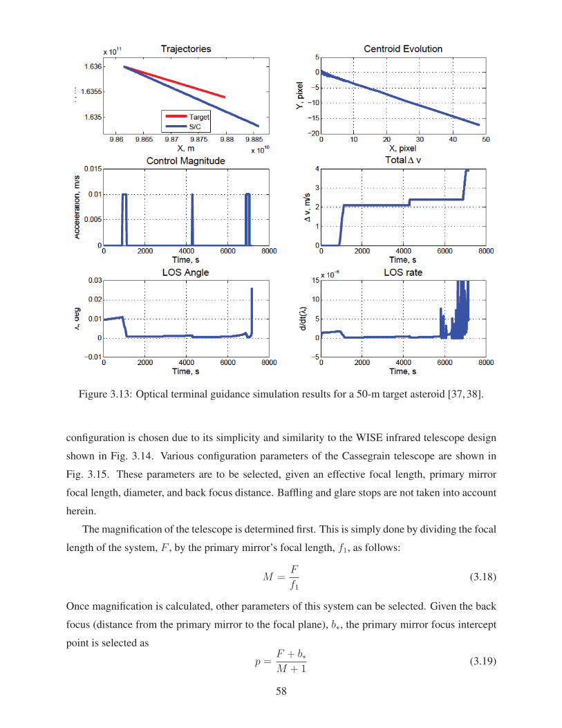
313 Optical terminal guidance simulation results for a 50-m target asteroid [37 38] 58
314 An illustration of WISE infrared space telescope (Image courtesy of NASAJPL) 59
315 Classical Cassegrain telescope configuration [39] 59
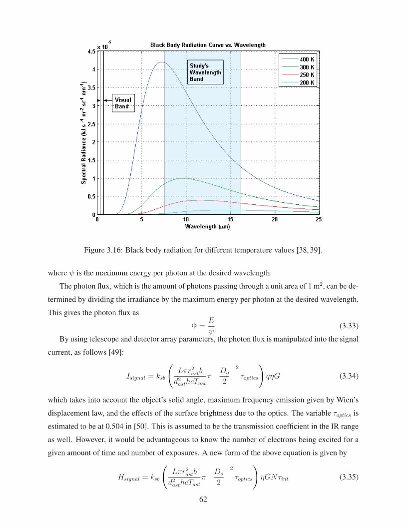
316 Black body radiation for different temperature values [38 39] 62
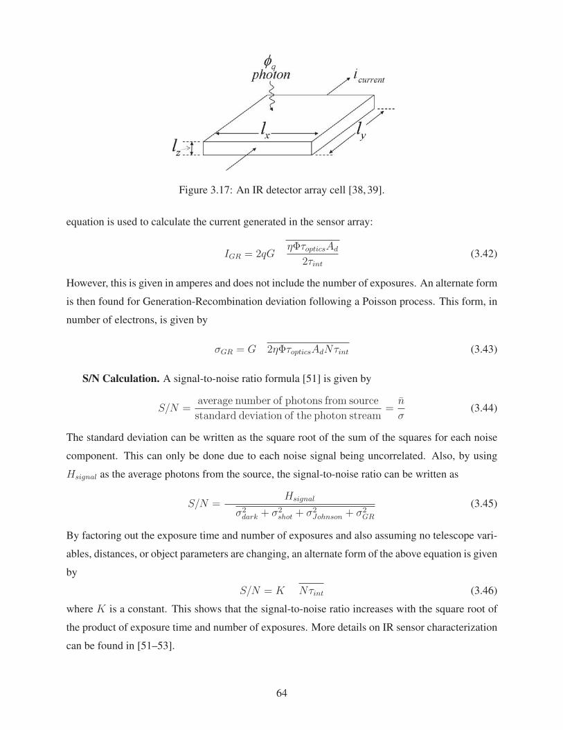
317 An IR detector array cell [38 39] 64
318 A reference Cassegrain IR telescope configuration for the HAIV mission [39] 67
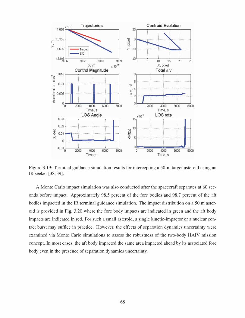
319 Terminal guidance simulation results for intercepting a 50-m target asteroid using
an IR seeker [38 39] 68
v
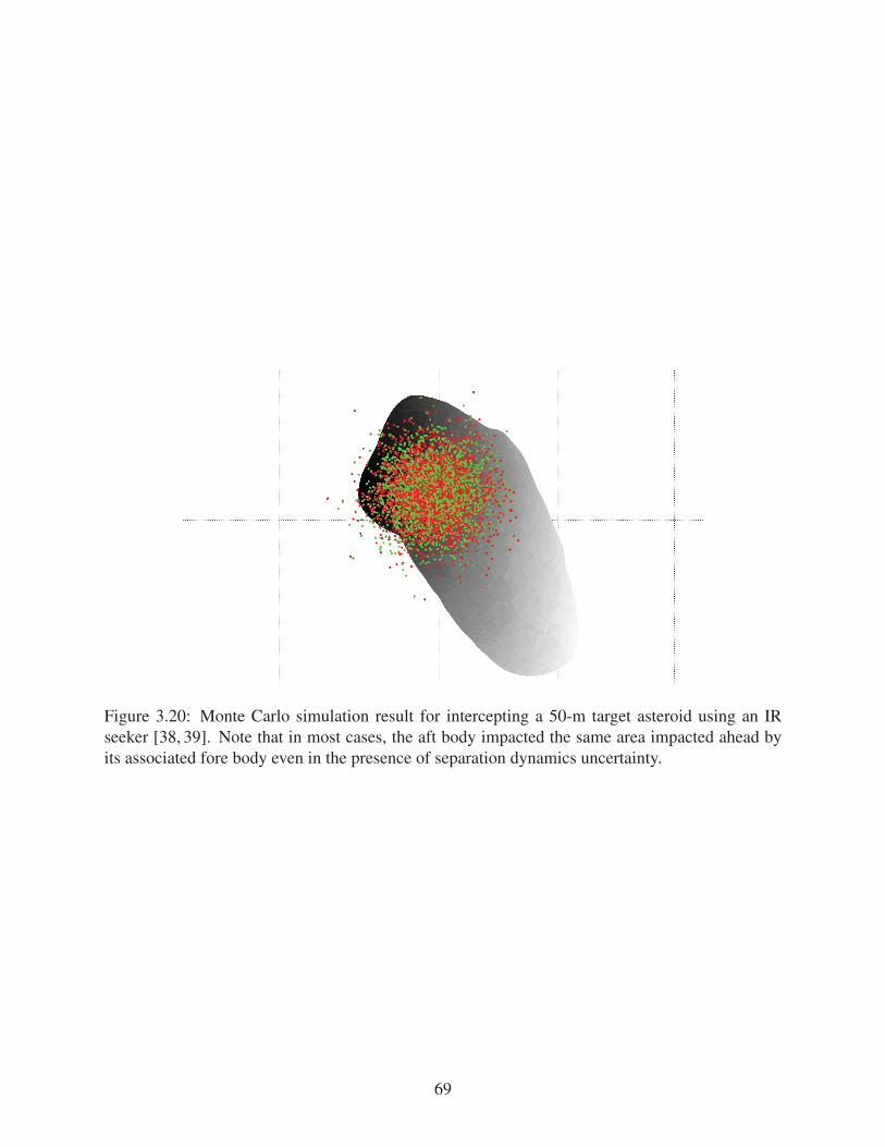
320 Monte Carlo simulation result for intercepting a 50-m target asteroid using an IR
seeker [38 39] Note that in most cases the aft body impacted the same area
impacted ahead by its associated fore body even in the presence of separation dyshy
namics uncertainty 69
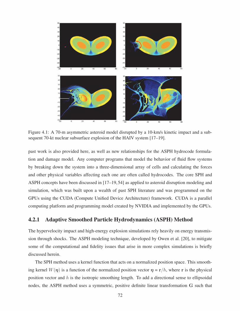
41 A 70-m asymmetric asteroid model disrupted by a 10-kms kinetic impact and a
subsequent 70-kt nuclear subsurface explosion of the HAIV system [17ndash19] 72
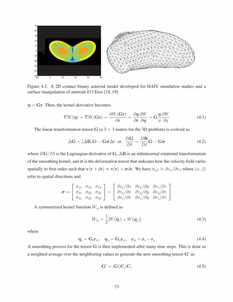
42 A 2D contact binary asteroid model developed for HAIV simulation studies and a
surface triangulation of asteroid 433 Eros [18 19] 73
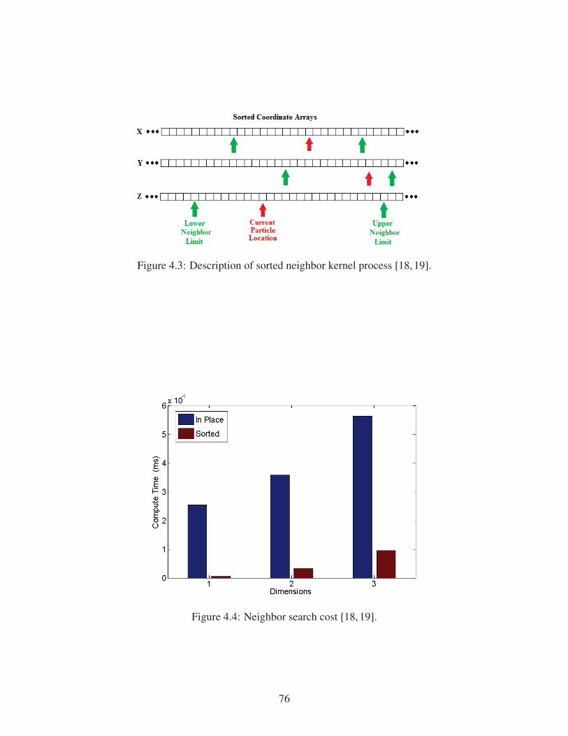
43 Description of sorted neighbor kernel process [18 19] 76
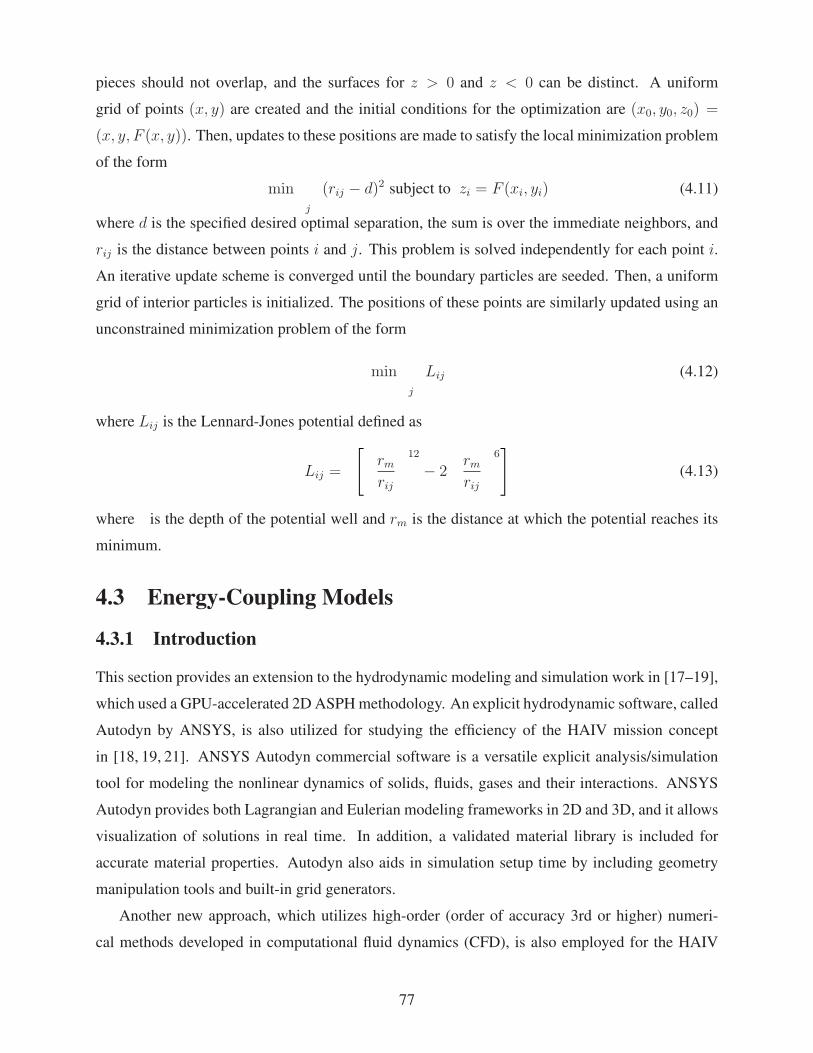
44 Neighbor search cost [18 19] 76
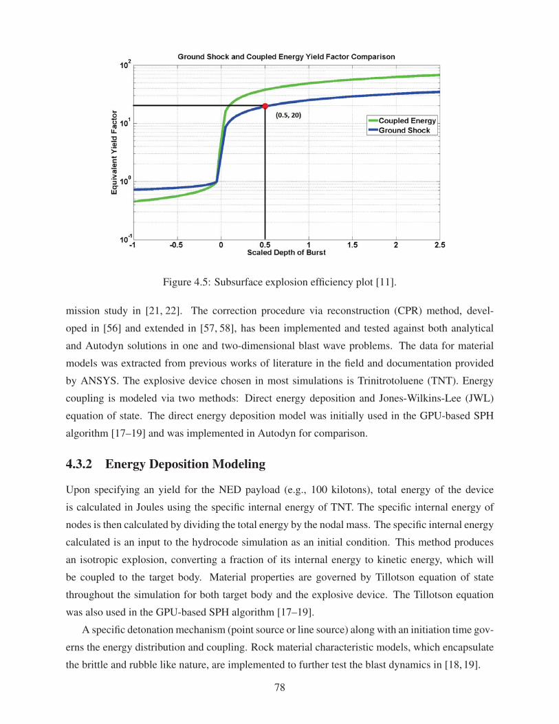
45 Subsurface explosion efficiency plot [11] 78
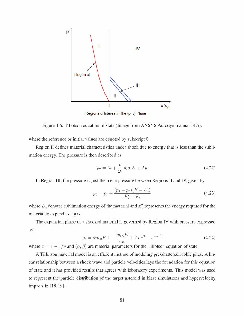
46 Tillotson equation of state (Image from ANSYS Autodyn manual 145) 81
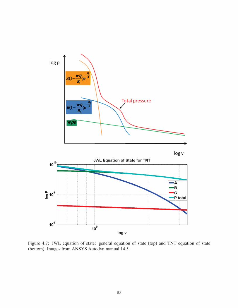
47 JWL equation of state general equation of state (top) and TNT equation of state
(bottom) Images from ANSYS Autodyn manual 145 83
48 Asymmetric shock behavior and disruption process for a 70-m asymmetric asteroid
[18 19] 85
49 Radial dispersion velocity histogram [18 19] 85
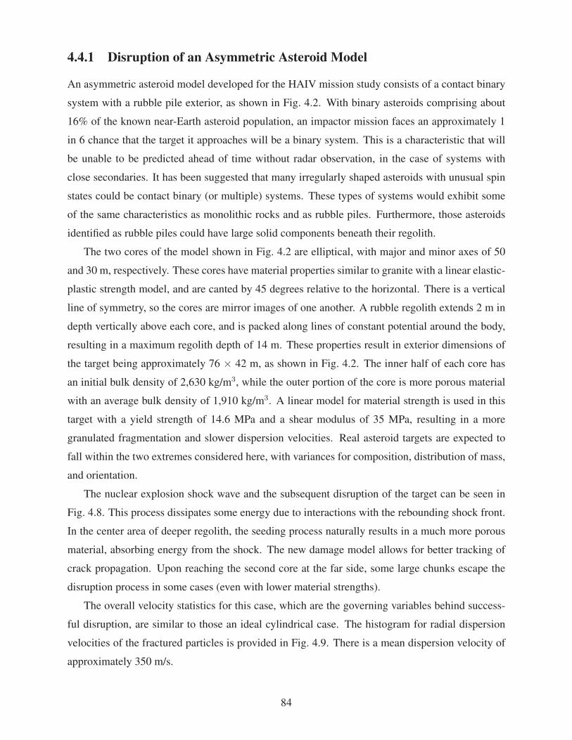
410 Final disruption of a target and location of slowest moving debris [18 19] The
color bar indicates the relative dispersion velocity distribution of slowest debris in
units of ms 86
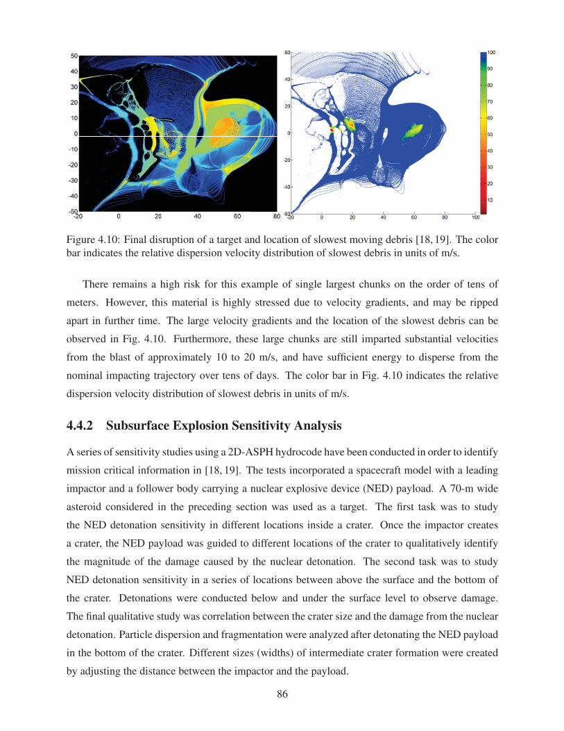
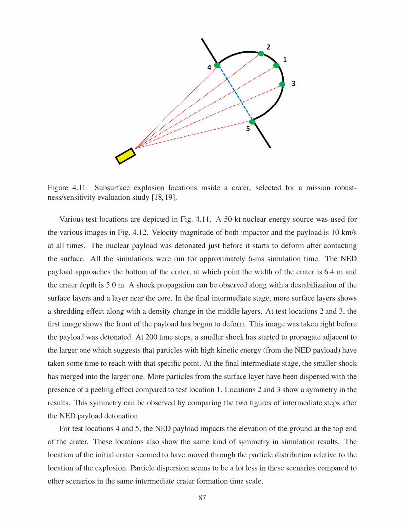
411 Subsurface explosion locations inside a crater selected for a mission robustnesssensitivity
evaluation study [18 19] 87
412 Simulation results for various subsurface explosion locations inside a crater [18 19] 88
413 Explosion locations for examining the nuclear detonation timing sensitivity 89
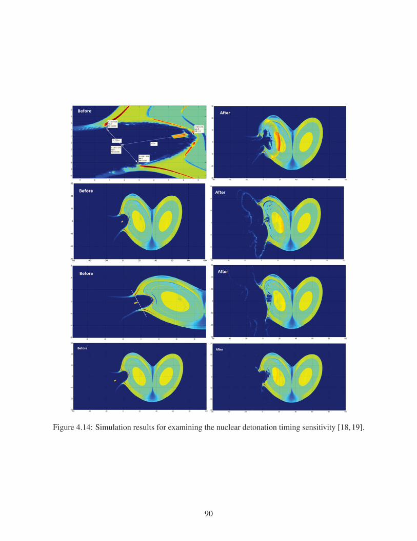
414 Simulation results for examining the nuclear detonation timing sensitivity [18 19] 90
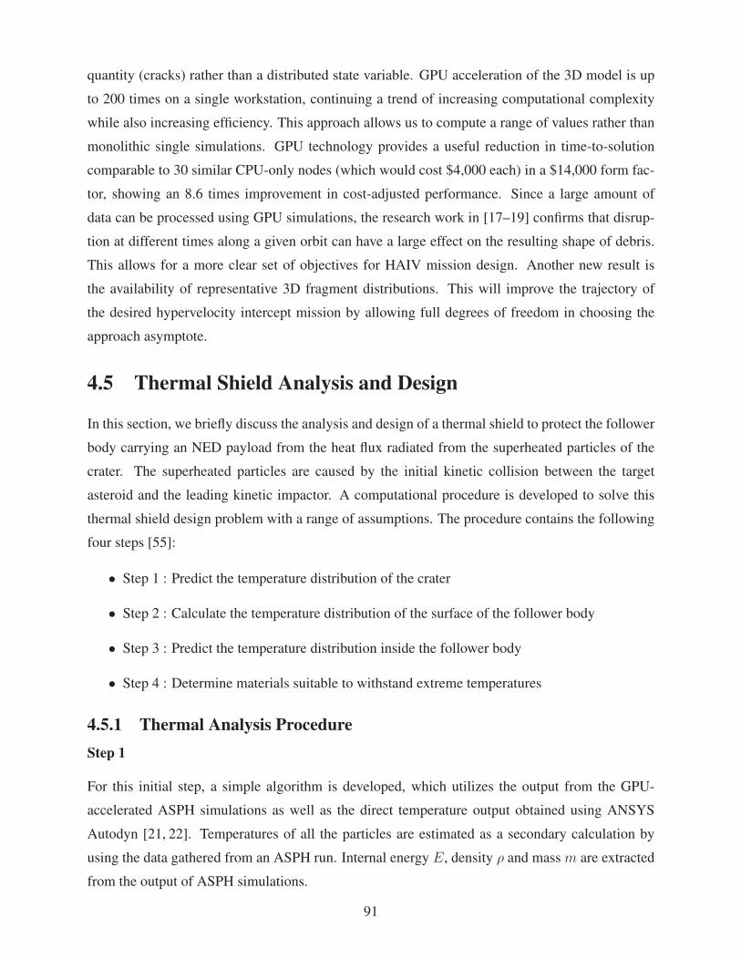
415 Nodal density (top) and temperature distribution in units of Kelvin (bottom) 93
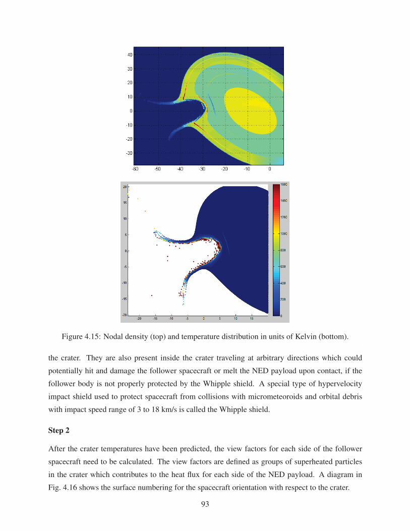
416 Surface numbering for the thermal analysis of a follower spacecraft carrying an
NED 94
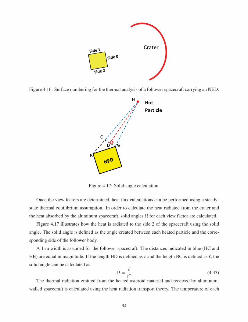
417 Solid angle calculation 94
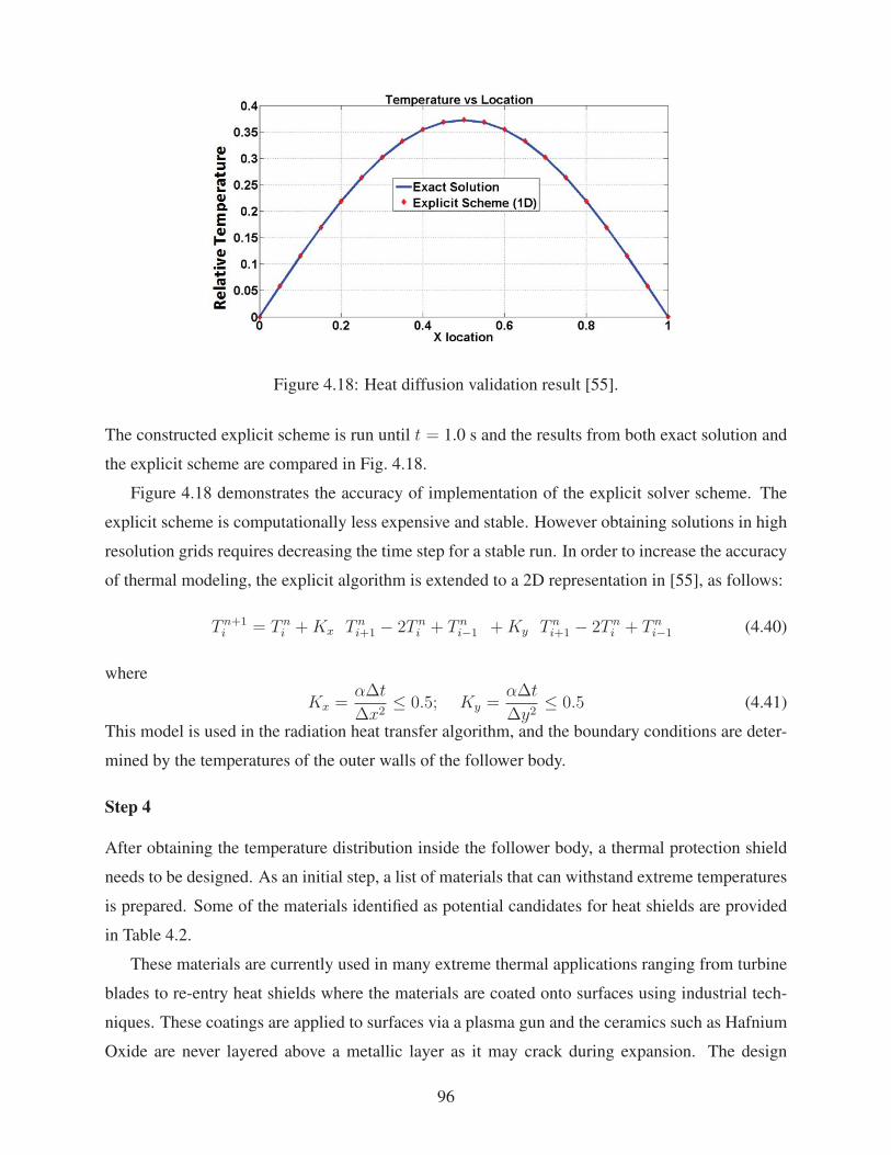
418 Heat diffusion validation result [55] 96
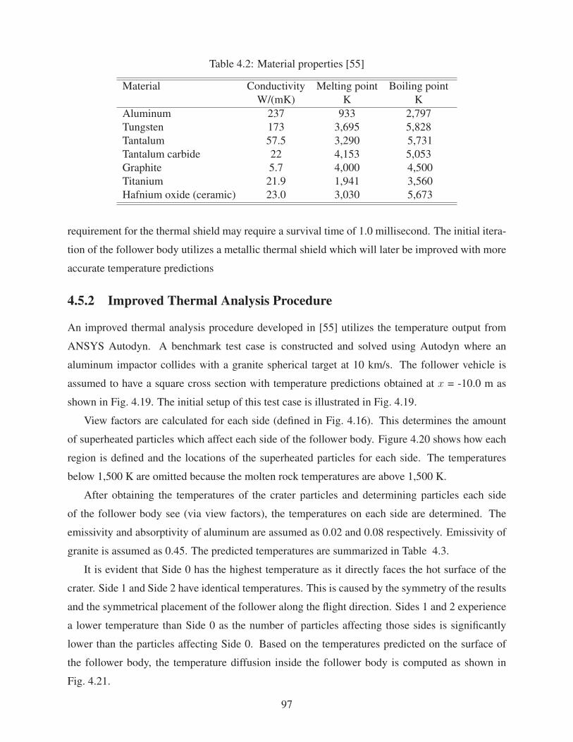
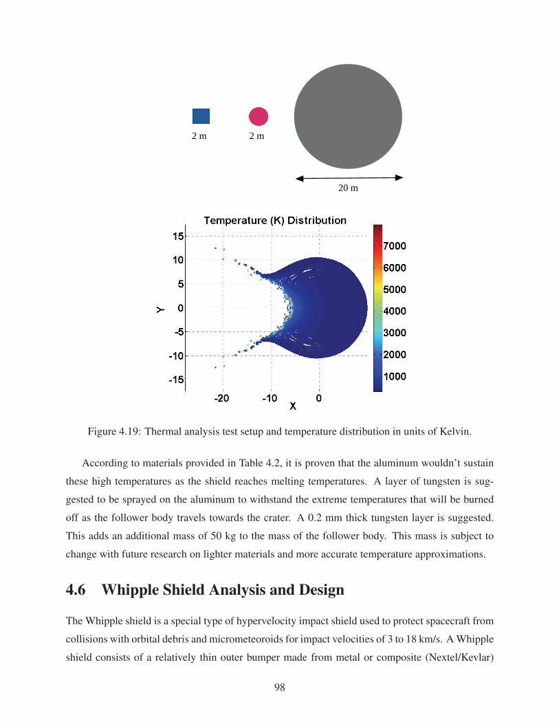
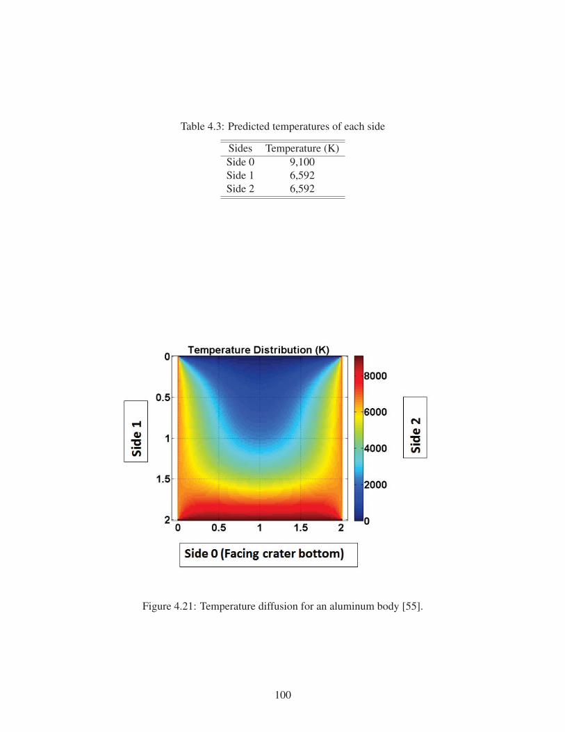
419 Thermal analysis test setup and temperature distribution in units of Kelvin 98
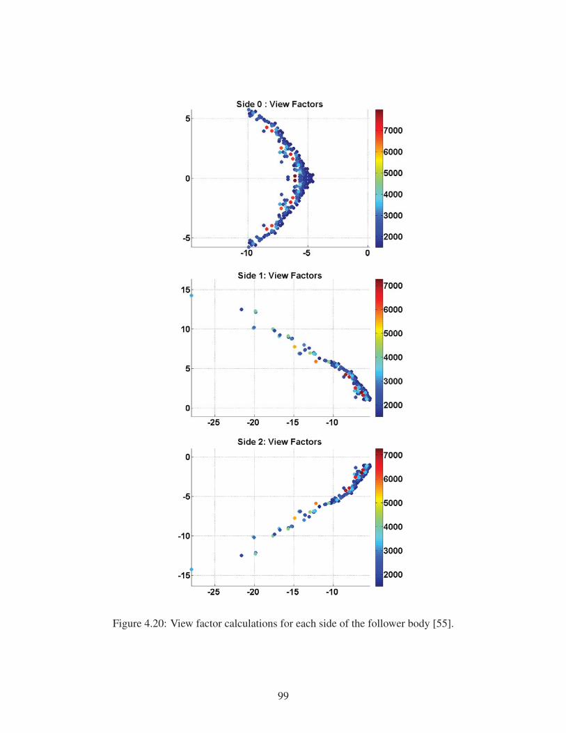
420 View factor calculations for each side of the follower body [55] 99
421 Temperature diffusion for an aluminum body [55] 100
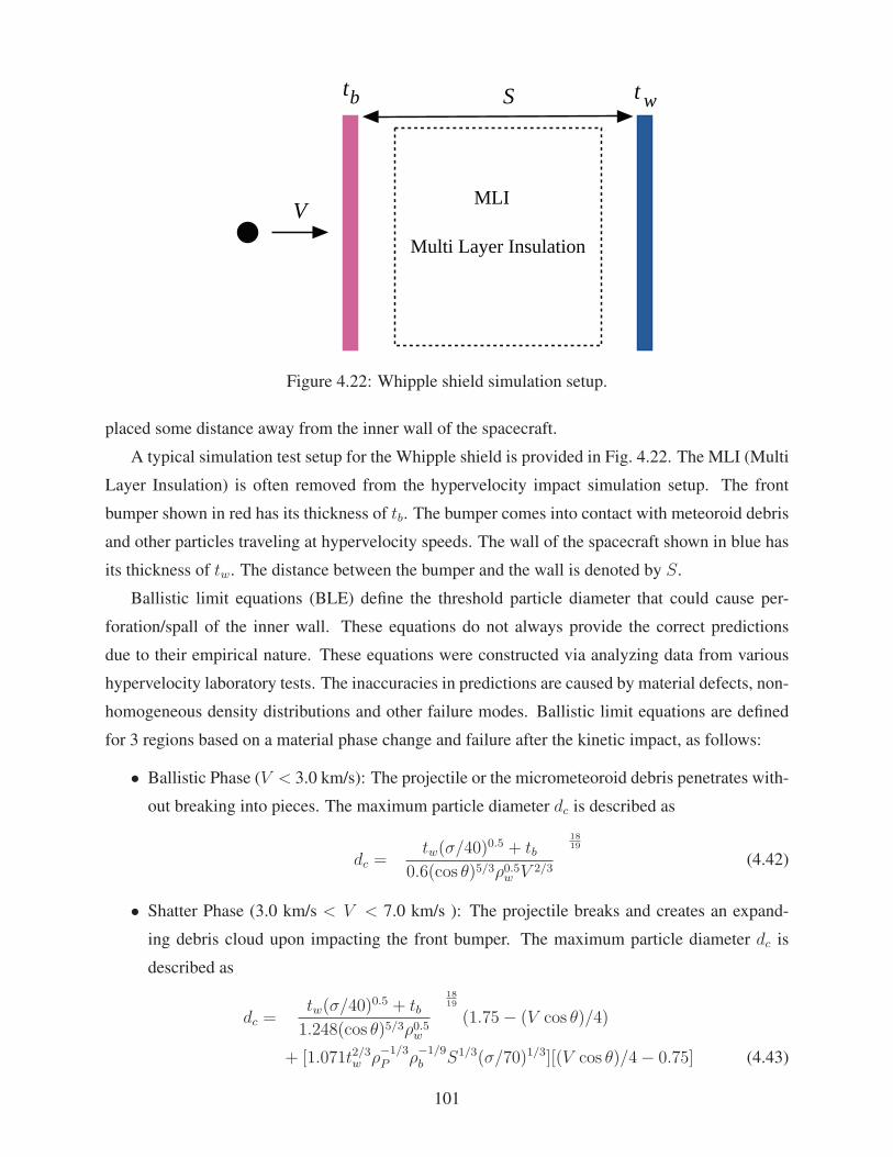
422 Whipple shield simulation setup 101
vi
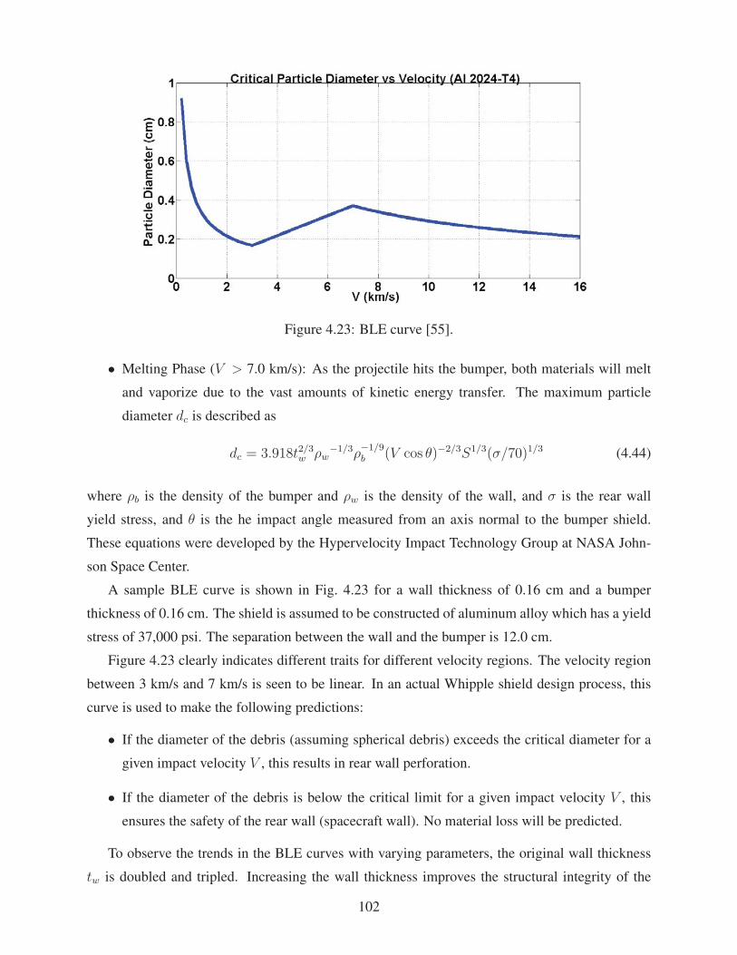
423 BLE curve [55] 102
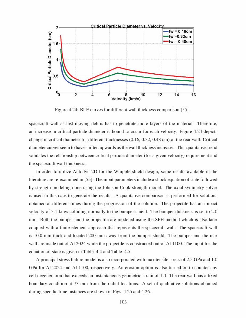
424 BLE curves for different wall thickness comparison [55] 103
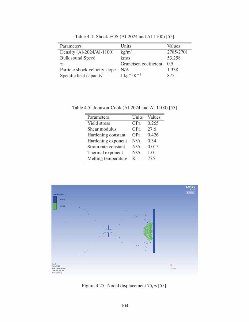
425 Nodal displacement 75μs [55] 104
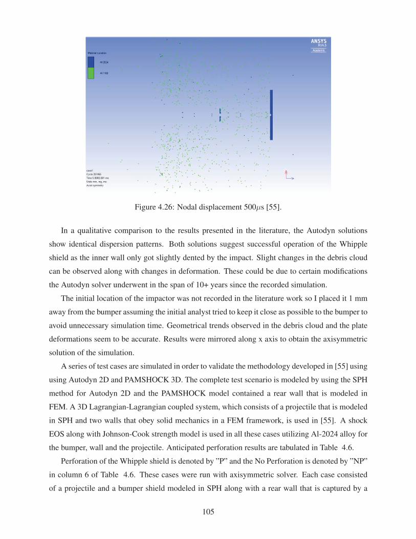
426 Nodal displacement 500μs [55] 105
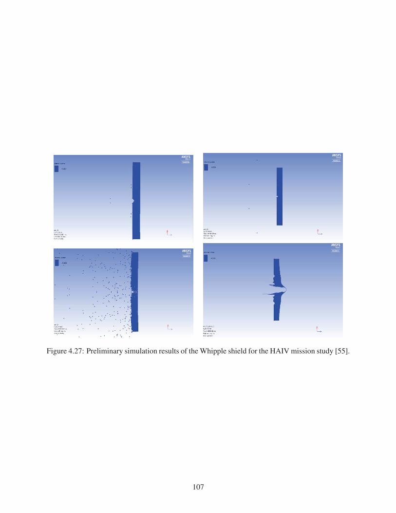
427 Preliminary simulation results of the Whipple shield for the HAIV mission study
[55] 107
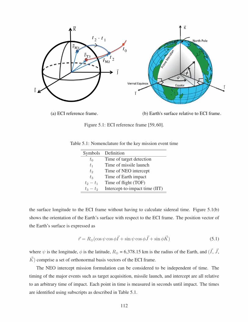
51 ECI reference frame [59 60] 112
52 Optimal intercept orbital geometry [59 60] 114
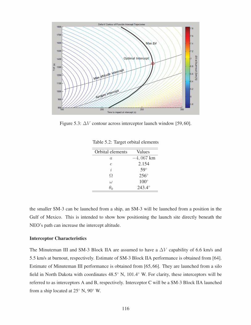
53 ΔV contour across interceptor launch window [59 60] 116
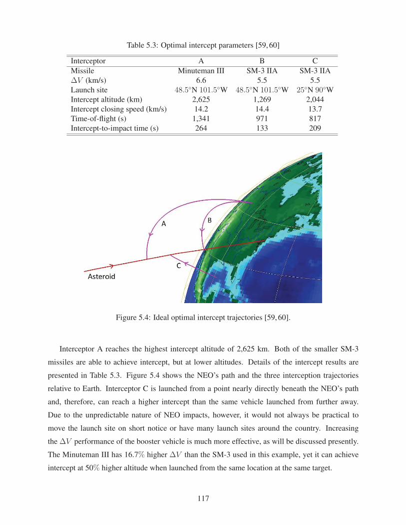
54 Ideal optimal intercept trajectories [59 60] 117
55 Notional planetary defense domes for the United States [59 60] 118
56 Late intercept trajectories [59 60] 119
61 Various orbits around asteroid 433 Eros [72ndash74] 126
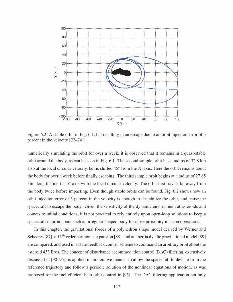
62 A stable orbit in Fig 61 but resulting in an escape due to an orbit injection error
of 5 percent in the velocity [72ndash74] 127
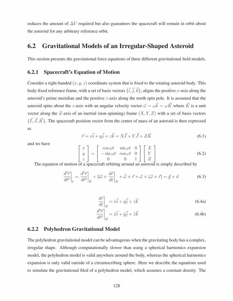
63 Illustration of a triangulated shape model of asteroid 433 Eros 129
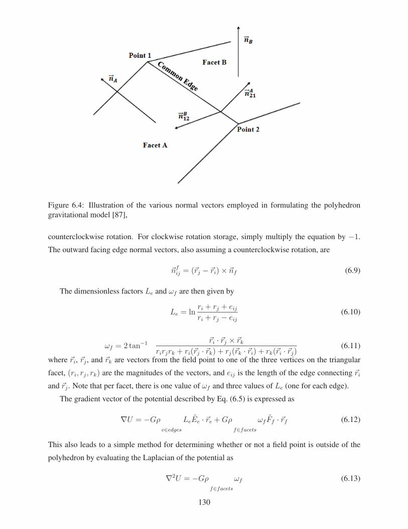
64 Illustration of the various normal vectors employed in formulating the polyhedron
gravitational model [87] 130
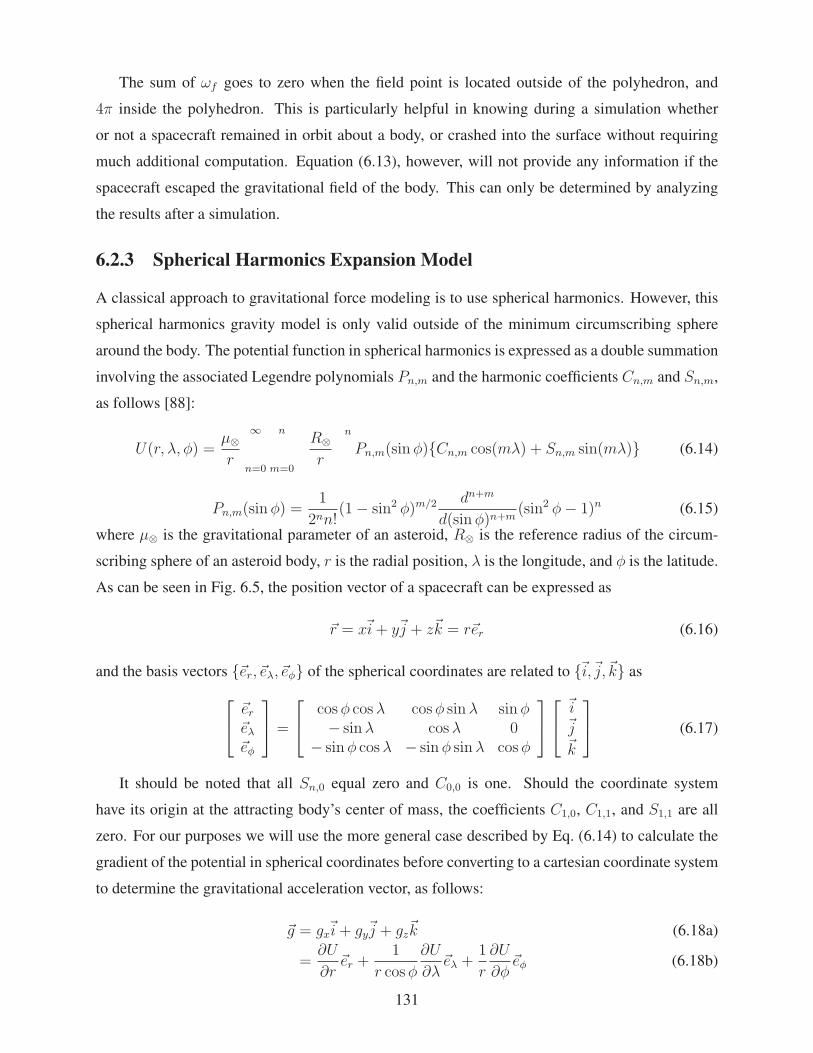
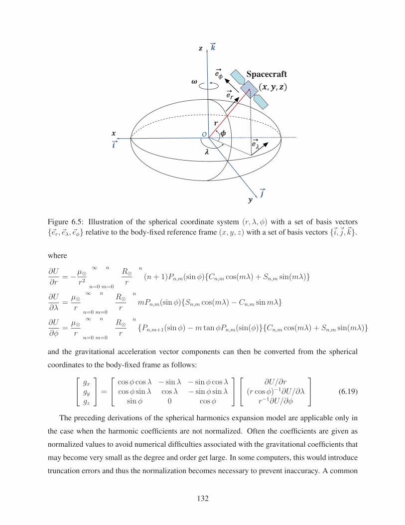
65 Illustration of the spherical coordinate system (r λ φ) with a set of basis vectors
eer eeλ eeφ relative to the body-fixed reference frame (x y z) with a set of basis
vectors e e ei j k 132
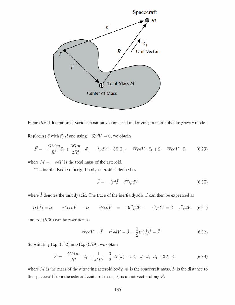
66 Illustration of various position vectors used in deriving an inertia dyadic gravity
model 135
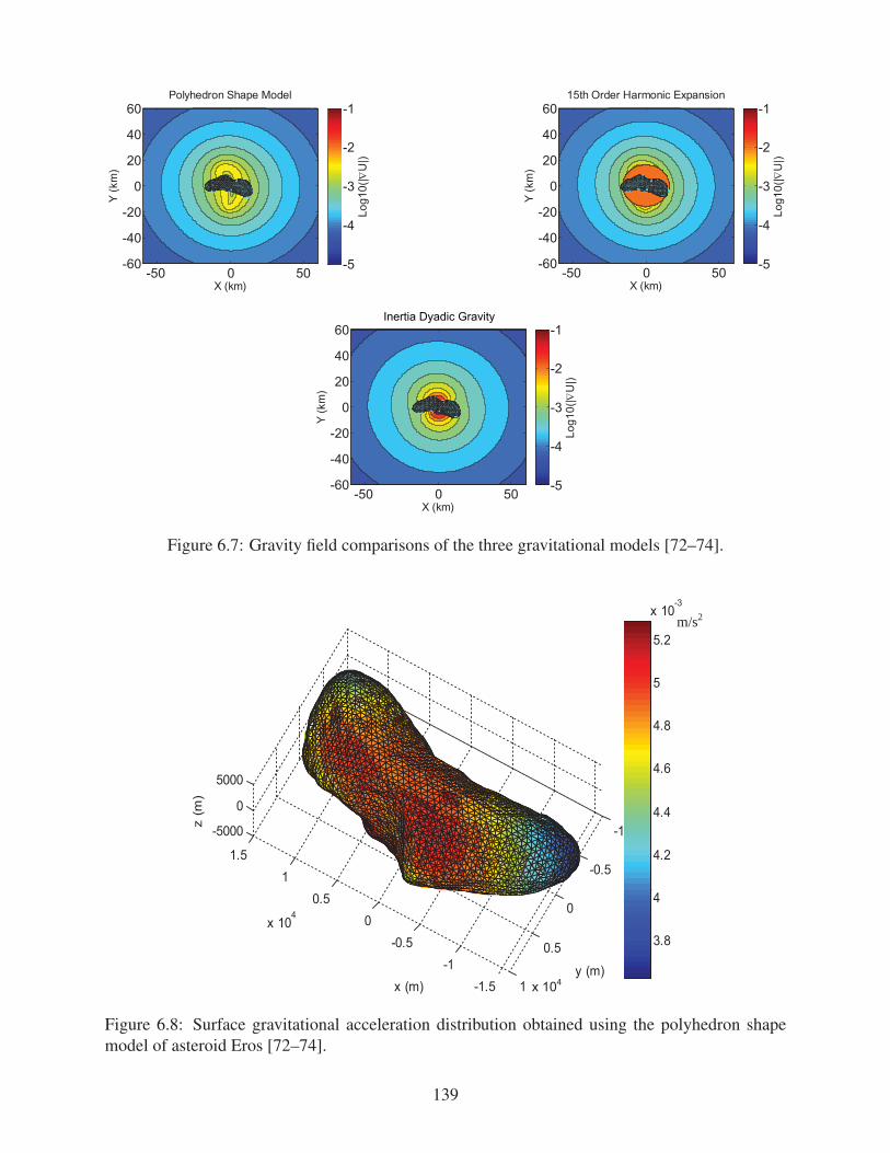
67 Gravity field comparisons of the three gravitational models [72ndash74] 139
68 Surface gravitational acceleration distribution obtained using the polyhedron shape
model of asteroid Eros [72ndash74] 139
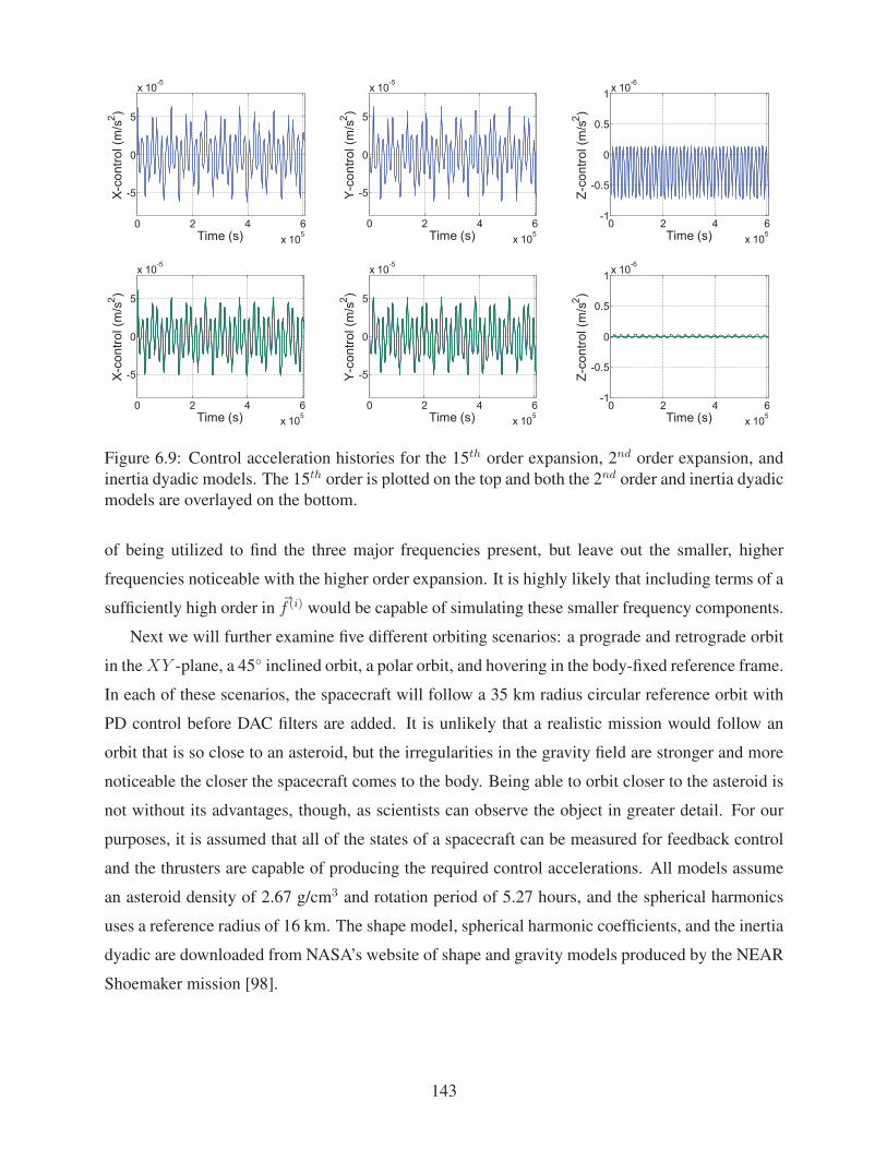
69 Control acceleration histories for the 15th order expansion 2nd order expansion
and inertia dyadic models The 15th order is plotted on the top and both the 2nd
order and inertia dyadic models are overlayed on the bottom 143
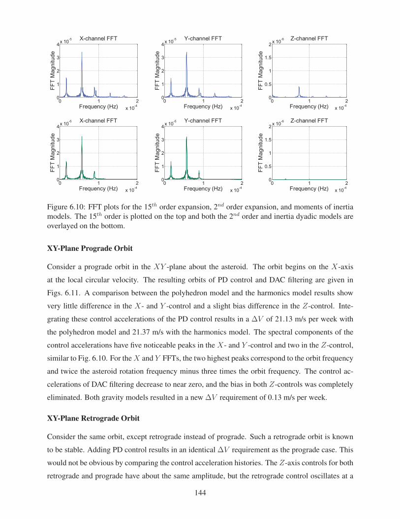
610 FFT plots for the 15th order expansion 2nd order expansion and moments of inershy
tia models The 15th order is plotted on the top and both the 2nd order and inertia
dyadic models are overlayed on the bottom 144
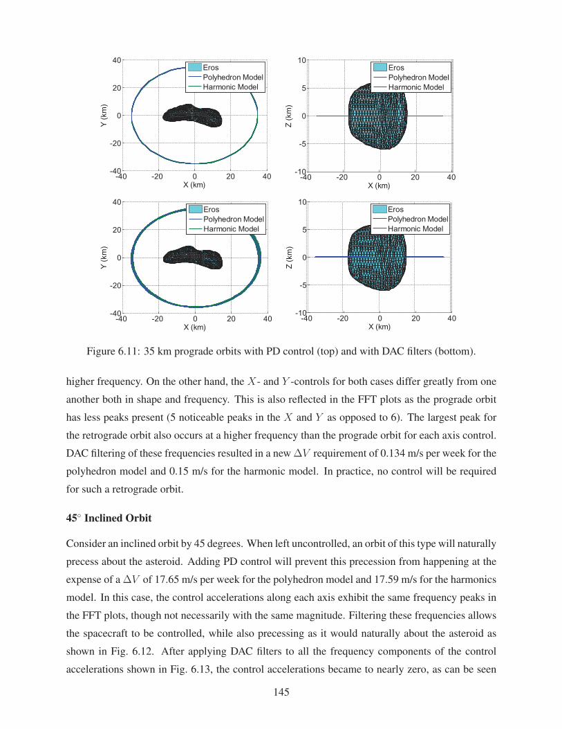
611 35 km prograde orbits with PD control (top) and with DAC filters (bottom) 145
vii
612 35 km inclined orbits with PD control (top) and DAC filters (bottom) 146
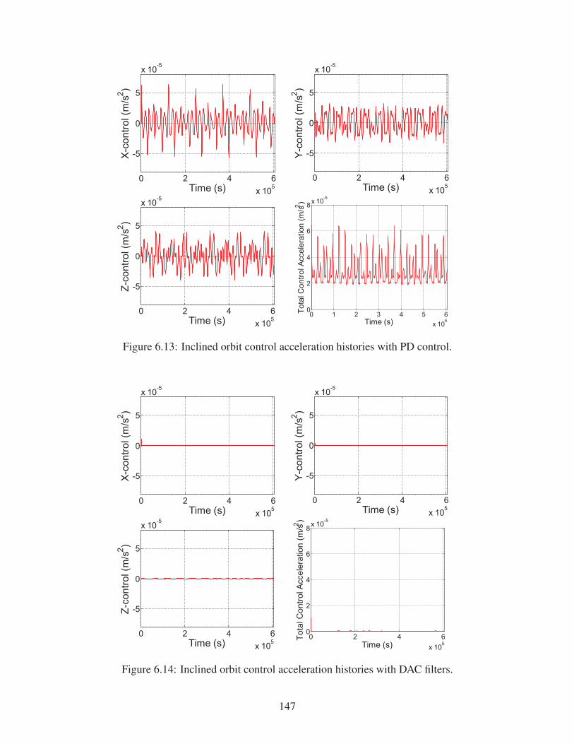
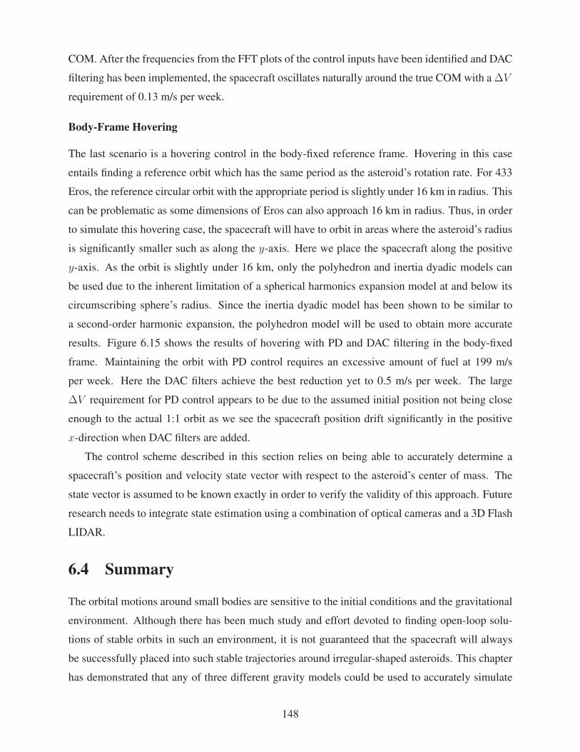
613 Inclined orbit control acceleration histories with PD control 147
614 Inclined orbit control acceleration histories with DAC filters 147
615 Hovering scenario with PD control and DAC filters 149
viii
List of Tables
21 Physical and orbital properties of a reference target (asteroid 2006 CL9) [15] 23
22 Notional flight validation mission selected for 2006 CL9 [15] 23
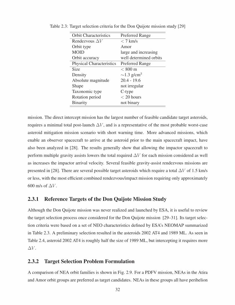
23 Target selection criteria for the Don Quijote mission study [29] 32
24 Properties of candidate targets formerly considered for the Don Quijote mission
study [29] 33
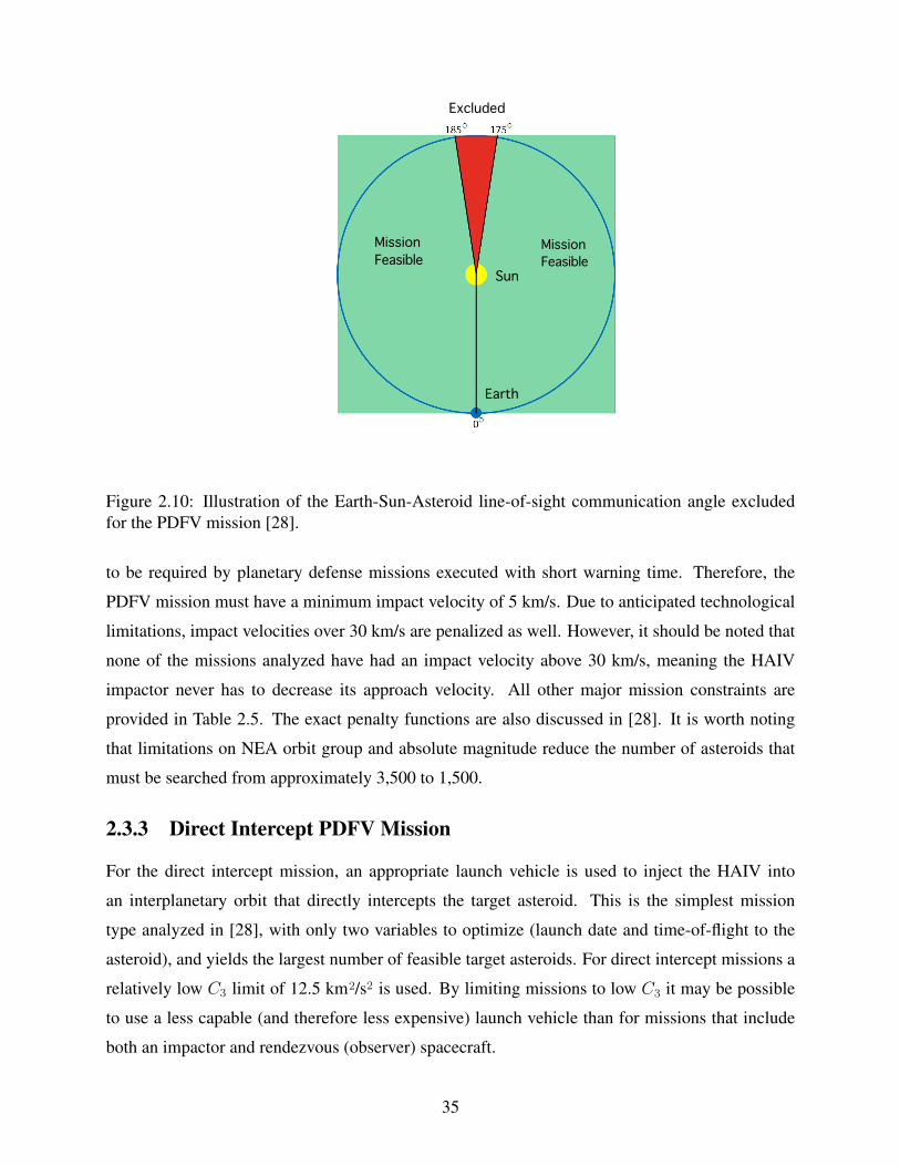
25 The PDFV mission constraints [28] 36
26 Top 3 target asteroid candidates for a simple direct intercept PDFV mission [28] 36
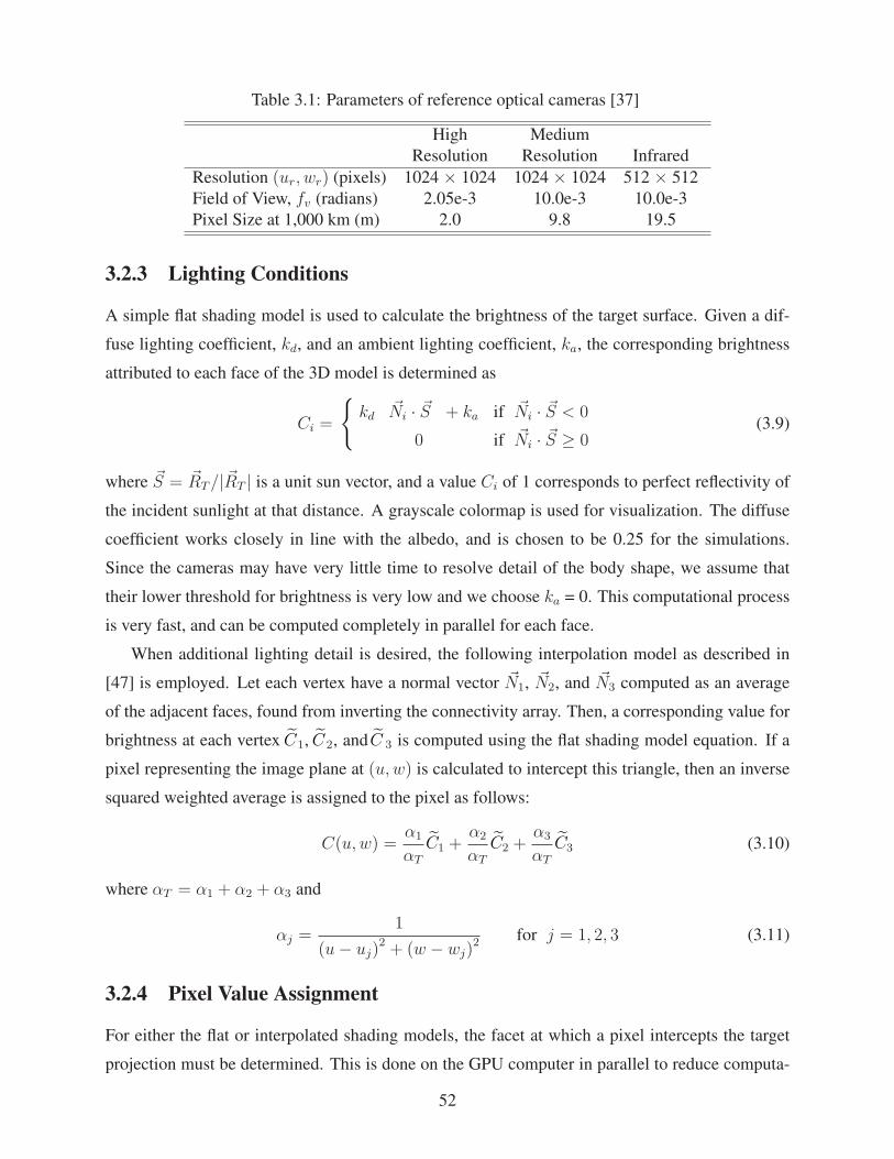
31 Parameters of reference optical cameras [37] 52
32 NEOWISE IR telescope characterization [39] 65
33 HAIV IR telescope characterization [39] 66
34 Performance of a reference IR telescopeseeker of the HAIV mission [39] 66
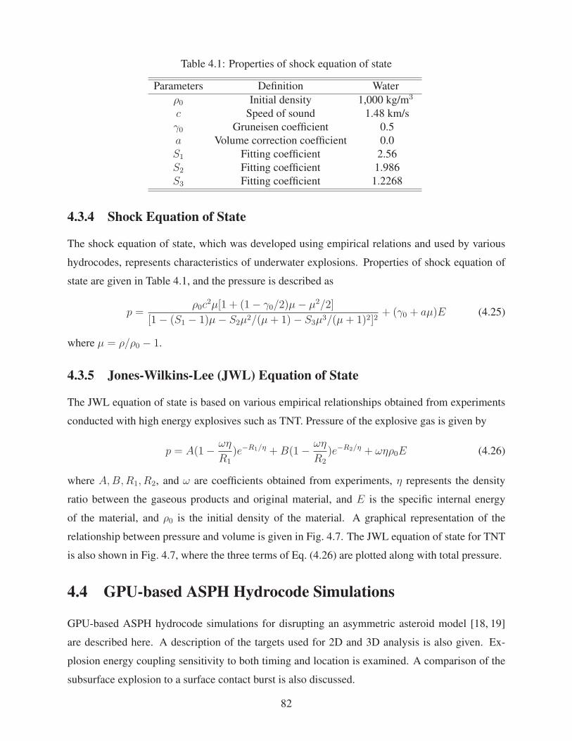
41 Properties of shock equation of state 82
42 Material properties [55] 97
43 Predicted temperatures of each side 100
44 Shock EOS (Al-2024 and Al-1100) [55] 104
45 Johnson-Cook (Al-2024 and Al-1100) [55] 104
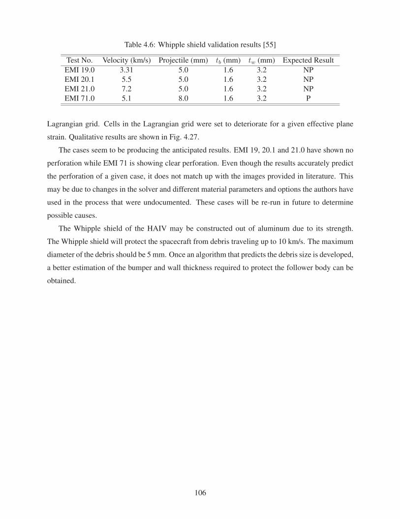
46 Whipple shield validation results [55] 106
51 Nomenclature for the key mission event time 112
52 Target orbital elements 116
53 Optimal intercept parameters [59 60] 117
54 Higher ΔV intercept scenarios [59 60] 120
55 Non-ballistic missile options [59 60] 120
56 Ballistic missile options [59 60] 121
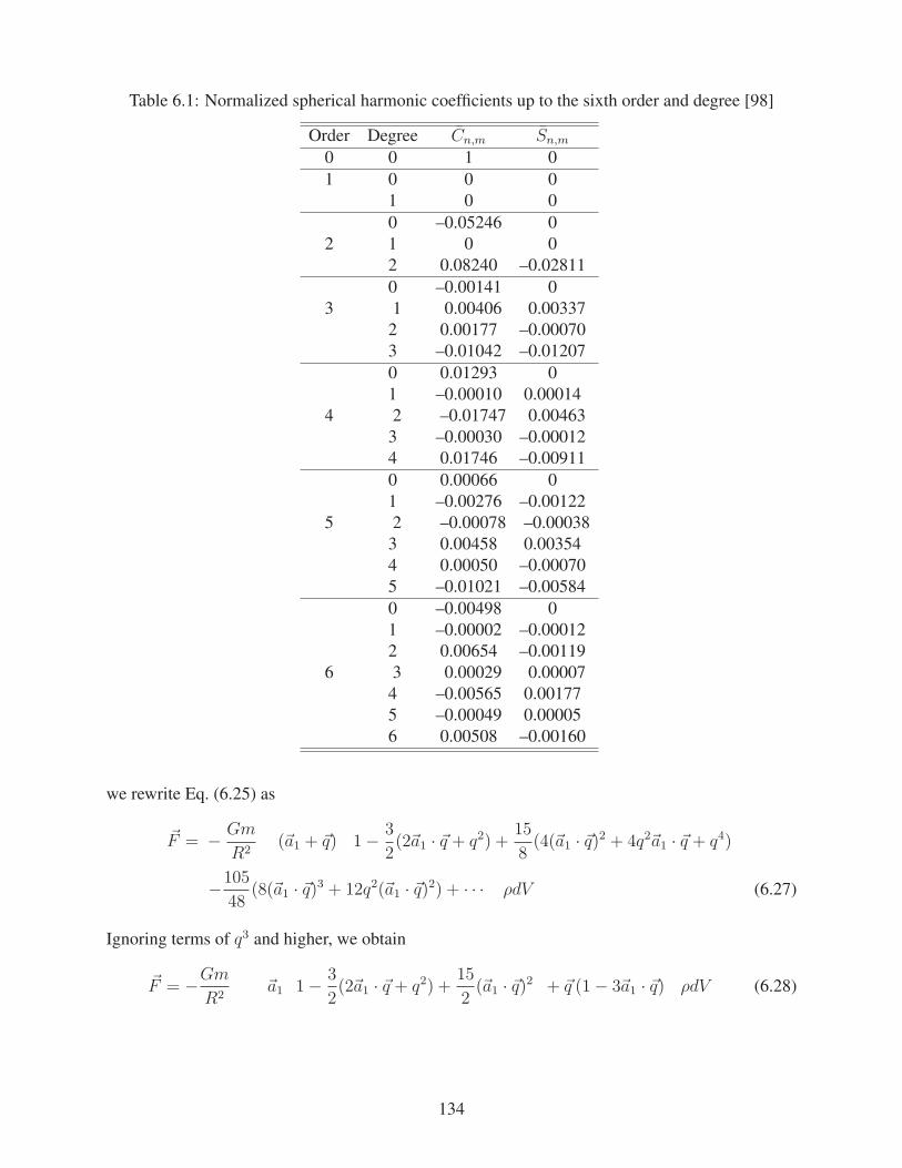
61 Normalized spherical harmonic coefficients up to the sixth order and degree [98] 134
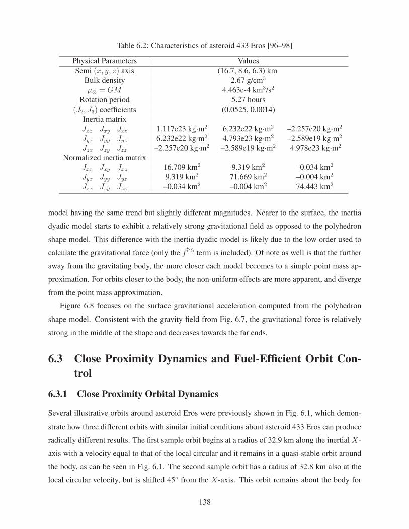
62 Characteristics of asteroid 433 Eros [96ndash98] 138
ix
Abstract
This final technical report describes the results of a NASA Innovative Advanced Concept
(NIAC) Phase 2 study entitled ldquoAn Innovative Solution to NASArsquos NEO Impact Threat Mitshy
igation Grand Challenge and Flight Validation Mission Architecture Developmentrdquo This
NIAC Phase 2 study was conducted at the Asteroid Deflection Research Center (ADRC)
of Iowa State University in 2012ndash2014 The study objective was to develop an innovative
yet practically implementable solution to the most probable impact threat of an asteroid or
comet with short warning time (lt5 years) The technical materials contained in this final reshy
port are based on numerous technical papers which have been previously published by the
project team of the NIAC Phase 1 and 2 studies during the past three years Those technical
papers as well as a NIAC Phase 2 Executive Summary report can be downloaded from the
ADRC website (wwwadrciastateedu)
1
Chapter 1
Hypervelocity Asteroid Intercept Vehicle (HAIV) Mission Concept
This chapter describes a planetary defense strategy that exploits the innovative concept of blendshy
ing a hypervelocity kinetic impactor with a subsurface nuclear explosion for mitigating the most
probable impact threat of near-Earth objects (NEOs) with a warning time shorter than 5 years
11 Introduction
Despite the lack of a known immediate impact threat from an asteroid or comet historical scienshy
tific evidence suggests that the potential for a major catastrophe created by an asteroid or comet
impacting Earth is very real Humankind must be prepared to deal with such an event that could
otherwise cause a regional or global catastrophe There is now growing national and international
interest in developing a global plan to protect the Earth from a catastrophic impact by a hazardous
near-Earth object (NEO) This growing interest was recently spurred by the Chelyabinsk meteorite
impact event that occurred in Russia on February 15 2013 and a near miss by asteroid 367943
Duende (2012 DA14) approximately 40 m in size on the same day
A variety of NEO deflectiondisruption technologies such as nuclear explosions kinetic imshy
pactors and slow-pull gravity tractors (GTs) have been investigated by planetary defense reshy
searchers during the past two decades [1ndash10] To date however there is no consensus on how
to reliably deflect or disrupt hazardous NEOs in a timely manner All of the non-nuclear techshy
niques will require mission lead times much longer than 10 years even for a relatively small NEO
When the time-to-impact with the Earth exceeds a decade the velocity perturbation needed to
alter the orbit of a target asteroid sufficiently to deflect it away from Earth impact is relatively
small (approximately 1 to 2 cms) Thus most non-nuclear options as well as a nuclear standshy
off explosion can be employed for deflection missions when we have sufficiently long warning
times It is emphasized that any NEO deflection effort must produce an actual orbital change much
2
larger than predicted orbital perturbation uncertainties from all sources Likewise any NEO deshy
flectiondisruption approach must be robust against the unknown material properties of a target
NEO
Kinetic impactors and nuclear explosions may be considered as the most mature technologies
for asteroid deflection or disruption as concluded in the 2010 NRC report [10] Both approaches
are impulsive and energy-rich in that the final momentum change can be considerably more than
that present in the original impactor or in the expanded vaporization layer (from a nuclear standoff
explosion) Both methods are expected to eject some debris and the amount depends on surface
material properties High porosity affects the ability to convert the excess energy into additional
momentum Some asteroids like Itokawa have been determined to have densities (and thus porosishy
ties) comparable to terrestrial material with well-characterized shock propagation Others appear
to have very low porosity that may absorb excess energy without the hydrodynamic rebound that
can amplify the original impulse
Because nuclear energy densities are nearly a million times higher than those possible with
chemical bonds a nuclear explosive device is the most mass-efficient means for storing energy with
todayrsquos technology Deflection methods with sufficiently high energy density are often preferred
over a nuclear disruption approach One of these deflection methods utilizes a nuclear explosion
at a specified standoff distance from the target NEO to effect a large velocity change by ablating
and blowing off a thin layer of the NEOrsquos surface Nuclear standoff explosions are thus assessed
to be much more effective than any other non-nuclear alternatives especially for larger asteroids
The precise outcome of a NEO deflection attempt using a nuclear standoff explosion is dependent
on myriad variables Shape and composition of the target NEO are critical factors These critical
properties plus others would need to be characterized ideally by a separate mission prior to a
successful nuclear deflection attempt Other techniques involving the use of surface or subsurface
nuclear explosives are assessed to be more efficient than the nuclear standoff explosion although
they may cause an increased risk of fracturing the target asteroid [10]
Nuclear standoff explosions require an optimal standoff distance for imparting maximum veshy
locity change to the target asteroid Therefore we have to determine how close the nuclear exploshy
sion must be to effectively change the orbital trajectories of asteroids of different types sizes and
shapes A simple model that can be used to assess the effectiveness of a nuclear standoff explosion
approach is developed in [9] Geometric principles and basic physics are used in [9] to construct a
simple model which can be augmented to account for icy bodies anisotropic ejecta distributions
and effects unique to the nuclear blast model Use of this simple model has resulted in an estimashy
tion of NEO velocity change of approximately 1 cms on the same order as other complex models
3
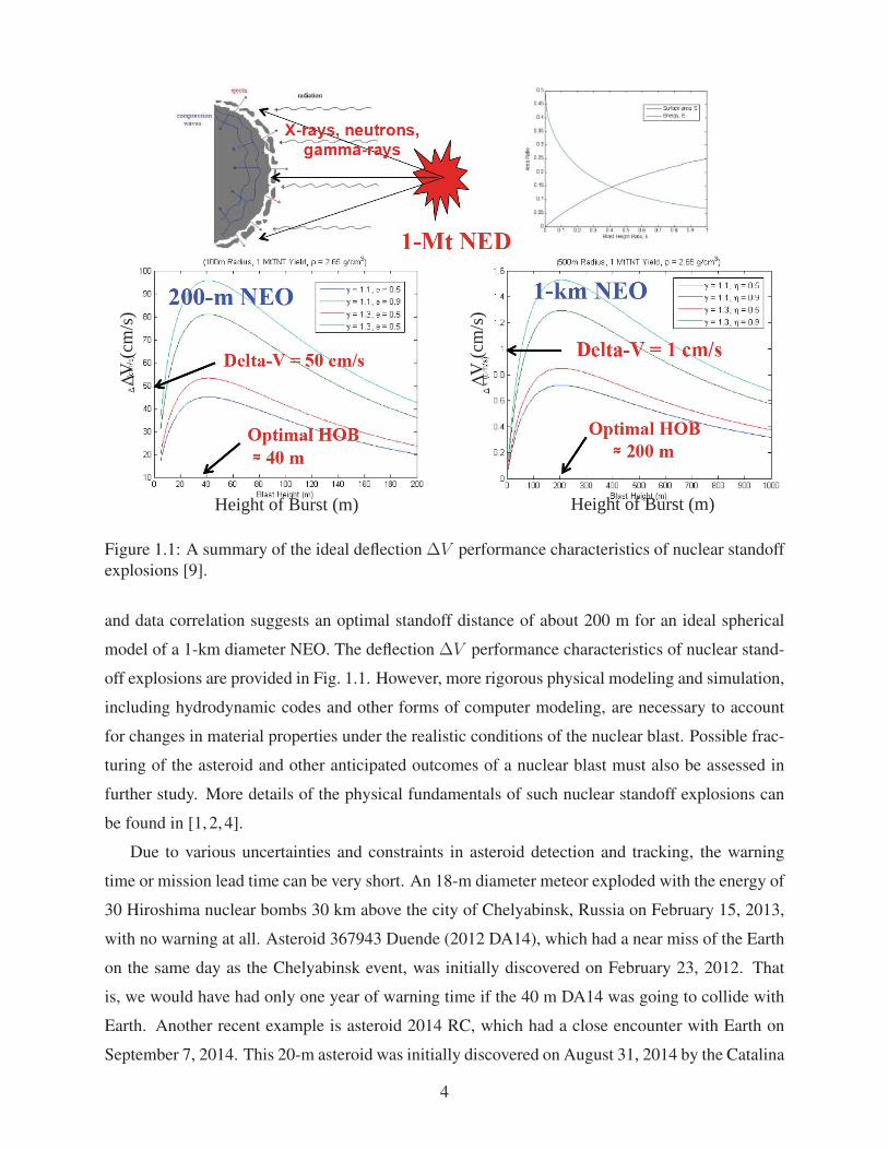
Figure 11 A summary of the ideal deflection ΔV performance characteristics of nuclear standoff
explosions [9]
and data correlation suggests an optimal standoff distance of about 200 m for an ideal spherical
model of a 1-km diameter NEO The deflection ΔV performance characteristics of nuclear standshy
off explosions are provided in Fig 11 However more rigorous physical modeling and simulation
including hydrodynamic codes and other forms of computer modeling are necessary to account
for changes in material properties under the realistic conditions of the nuclear blast Possible fracshy
turing of the asteroid and other anticipated outcomes of a nuclear blast must also be assessed in
further study More details of the physical fundamentals of such nuclear standoff explosions can
be found in [1 2 4]
Due to various uncertainties and constraints in asteroid detection and tracking the warning
time or mission lead time can be very short An 18-m diameter meteor exploded with the energy of
30 Hiroshima nuclear bombs 30 km above the city of Chelyabinsk Russia on February 15 2013
with no warning at all Asteroid 367943 Duende (2012 DA14) which had a near miss of the Earth
on the same day as the Chelyabinsk event was initially discovered on February 23 2012 That
is we would have had only one year of warning time if the 40 m DA14 was going to collide with
Earth Another recent example is asteroid 2014 RC which had a close encounter with Earth on
September 7 2014 This 20-m asteroid was initially discovered on August 31 2014 by the Catalina
4
Height of Burst (m) Height of Burst (m)
ΔV(c
ms
)
ΔV(c
ms
)
Sky Survey near Tucson Arizona and independently detected the next night by the Pan-STARRS
1 telescope located on the summit of Haleakala on Maui Hawaii We would have had only one
week of warning time if 2014 RC was going to collide with Earth
If a NEO on an Earth-impacting course is detected with a short warning time (eg much less
than 5 years) the challenge becomes how to mitigate its threat in a timely manner For a small
asteroid impacting in a sufficiently unpopulated region mitigation may simply involve evacuation
[10] However for larger asteroids or asteroids impacting sufficiently developed regions the
threat may be mitigated by either disrupting the asteroid (ie destroying or fragmenting with
substantial orbital dispersion) or by altering its trajectory such that it will either avoid impacting
the predicted impact location or miss the Earth entirely When the time to impact with Earth is
short the velocity change required to deflect an NEO becomes extremely large Thus for the most
probable mission scenarios in which the warning time is shorter than 5 years the use of high-
energy nuclear explosives in space will become inevitable [10] A scenario in which a small (eg
50 to 150 m) Earth-impacting NEO is discovered with short warning time is considered the most
probable scenario because smaller NEOs greatly outnumber larger NEOs and smaller NEOs are
more difficult to detect Most direct intercept missions with a short warning time will result in
arrival closing velocities of 10 to 30 kms with respect to a target asteroid A rendezvous mission
to a target asteroid that requires such an extremely large arrival ΔV of 10 to 30 kms is not feasible
A subsurface nuclear explosion is the most efficient use of nuclear explosives [10 11] The
nuclear subsurface explosion even with shallow burial to a depth of 3 to 5 m can deliver a large
amount of energy into the target asteroid so that there is a likelihood of totally disrupting the target
asteroid Such subsurface nuclear explosions are known to be at least 20 times more effective than
a nuclear contact burst (a nuclear explosion very close to the surface) [11] The momentumenergy
transfer created by a shallow subsurface nuclear explosion is at least 100 times larger than that
of an optimal standoff nuclear explosion However state-of-the-art nuclear subsurface penetrator
technology limits the impact velocity to no more than about 300 ms because higher impact veshy
locities prematurely destroy the fusing mechanismselectronics of nuclear explosive devices [11]
An increased impact speed limit of 15 kms may be technically feasible as mentioned in [11] for
nuclear Earth-Penetrator Weapons (EPWs) Neither a precision standoff explosion at an optimal
height of burst near an irregularly shaped smaller NEO with intercept velocities as high as 30
kms nor a surface contact burst is a trivial engineering task
Despite the uncertainties inherent to the nuclear disruption approach disruption can become
an effective strategy if most fragments disperse at speeds in excess of the escape velocity of an
asteroid so that a very small fraction of fragments impacts the Earth When the warning time
5
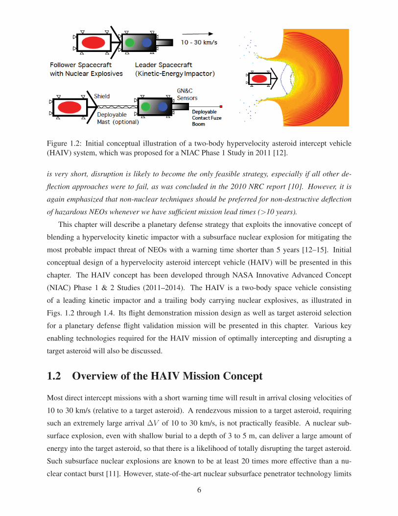
Figure 12 Initial conceptual illustration of a two-body hypervelocity asteroid intercept vehicle
(HAIV) system which was proposed for a NIAC Phase 1 Study in 2011 [12]
is very short disruption is likely to become the only feasible strategy especially if all other deshy
flection approaches were to fail as was concluded in the 2010 NRC report [10] However it is
again emphasized that non-nuclear techniques should be preferred for non-destructive deflection
of hazardous NEOs whenever we have sufficient mission lead times (gt10 years)
This chapter will describe a planetary defense strategy that exploits the innovative concept of
blending a hypervelocity kinetic impactor with a subsurface nuclear explosion for mitigating the
most probable impact threat of NEOs with a warning time shorter than 5 years [12ndash15] Initial
conceptual design of a hypervelocity asteroid intercept vehicle (HAIV) will be presented in this
chapter The HAIV concept has been developed through NASA Innovative Advanced Concept
(NIAC) Phase 1 amp 2 Studies (2011ndash2014) The HAIV is a two-body space vehicle consisting
of a leading kinetic impactor and a trailing body carrying nuclear explosives as illustrated in
Figs 12 through 14 Its flight demonstration mission design as well as target asteroid selection
for a planetary defense flight validation mission will be presented in this chapter Various key
enabling technologies required for the HAIV mission of optimally intercepting and disrupting a
target asteroid will also be discussed
12 Overview of the HAIV Mission Concept
Most direct intercept missions with a short warning time will result in arrival closing velocities of
10 to 30 kms (relative to a target asteroid) A rendezvous mission to a target asteroid requiring
such an extremely large arrival ΔV of 10 to 30 kms is not practically feasible A nuclear subshy
surface explosion even with shallow burial to a depth of 3 to 5 m can deliver a large amount of
energy into the target asteroid so that there is a likelihood of totally disrupting the target asteroid
Such subsurface nuclear explosions are known to be at least 20 times more effective than a nushy
clear contact burst [11] However state-of-the-art nuclear subsurface penetrator technology limits
6
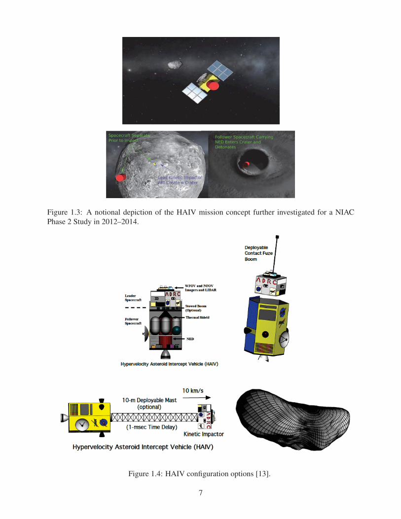
Figure 13 A notional depiction of the HAIV mission concept further investigated for a NIAC
Phase 2 Study in 2012ndash2014
7
Figure 14 HAIV configuration options [13]
Launch Vehicles
Nuclear Explosive Device (NED)
Terminal Guidance Begins Impact - 2 hrs
for 50- to 150-m target
Target Aquisition
Delta II Class
Figure 15 A reference HAIV flight system and its terminal guidance operational concept [13]
the impact velocity to less than about 300 ms because higher impact velocities prematurely deshy
stroy the fusing mechanismselectronics of nuclear explosive devices [11] That said an increased
impact speed limit of 15 kms may be technically feasible as mentioned in [11] for nuclear Earth-
Penetrator Weapons (EPWs)
In order to overcome such practical constraints on the penetrated subsurface nuclear explosion
a hypervelocity asteroid intercept vehicle (HAIV) system concept has been developed The HAIV
system will enable a last-minute nuclear disruption mission with intercept velocities as high as 30
kms The HAIV is a two-body space vehicle consisting of a fore body (leader) and an aft body
(follower) as illustrated in Figs 12 through 14 The leader spacecraft creates a kinetic-impact
crater in which the follower spacecraft carrying nuclear explosive devices (NEDs) makes a robust
and effective explosion below the surface of the target asteroid body Surface contact burst or
standoff explosion missions will not require such a two-body vehicle configuration However for
a precision standoff explosion at an optimal height of burst accurate timing of the nuclear explosive
detonation will be required during the terminal guidance phase of hypervelocity intercept missions
A reference HAIV mission architecture and its terminal guidance phase are illustrated in Fig 15
For a small (50 to 150 m) target asteroid the terminal guidance phase may begin 2 hrs prior to
the final intercept collision The nuclear fuzing system may be activated arming the NED payshy
load much earlier in the terminal phase operations timeline Instruments located on the leader
8
spacecraft detect the target NEO and a terminal guidance subsystem on-board the HAIV becomes
active Measurements continue through opticalIR cameras located on the leader spacecraft and an
intercept impact location is identified on the target asteroid body The high-resolution opticalIR
cameras provide successive images of the NEO to the terminal guidance system for a few trajecshy
tory correction maneuvers (TCMs) Separation must occur between the leader spacecraft and the
follower spacecraft before the leading kinetic impactor collides with the target
A variety of existing launch vehicles such as Delta II class Atlas V Delta IV and Delta IV
Heavy can be used for the HAIV mission carrying a variety of NED payloads ranging from 300shy
kg (with approximately 300-kt yield) to 1500-kg (with approximately 2-Mt yield) Conceptual
design of an interplanetary ballistic missile (IPBM) system architecture for launching the HAIV
system can be found in [16]
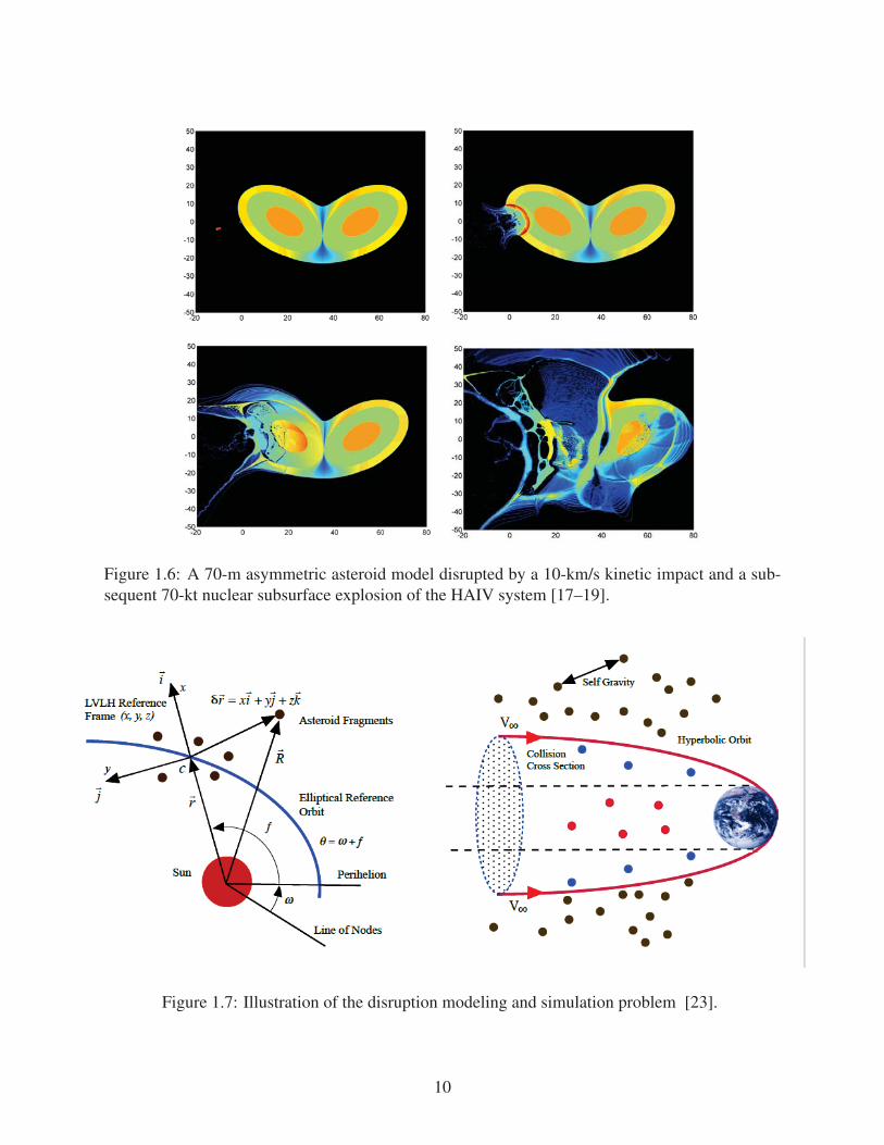
Because the hypervelocity kinetic impact and nuclear subsurface explosion simulations rely
heavily on energy transmission through shocks the simulation research work conducted for the
HAIV mission concept study [17ndash19] used Adaptive Smoothed Particle Hydrodynamics (ASPH)
to mitigate some of the computational and fidelity issues that arise in more complex high-fidelity
hydrocode simulations The propagation of the nuclear explosive shock can be seen for an illusshy
trative benchmark test case shown in Fig 16 The shock propagation process dissipates some
energy due to interactions with the rebounding shock front In the center area of deeper regolith
the seeding process naturally results in a much more porous material absorbing energy from the
shock Upon reaching the second core at the far side some large chunks escape the disruption proshy
cess in some cases (even with lower material strengths) An improved ASPH code implemented
on a modern low-cost GPU (Graphics Processing Unit) desktop computer has been developed for
the HAIV mission study [17ndash19] using the research results of Owen et al [20] However a more
computationally efficient modern GPU-based hydrodynamics code needs to be further developed
by incorporating more accurate physical models of a nuclear subsurface explosion [2122] Details
of nuclear subsurface explosion modeling and simulations will be presented in Chapter 4
The orbital dispersion problem of a fragmented asteroid in an elliptic orbit for assessing the
effectiveness of an asteroid disruption mission is illustrated in Fig 17 [23] Various approaches
have been employed in [23] to be computationally efficient and accurate for several examples with
a large number of fragments (eg 500000) An N-body orbit simulation code was also used for
orbital dispersion simulation and analysis in [23 24] To assess the degree of mitigation the code
includes the gravitational focusing effect of the Earth on those fragments that pass near the Earth
and provides a census of those that hit the Earth (ie those fragment with a minimum distance to
Earth of lt1 Earth radius) The code then has two modes of use as described as [23 24]
9
10
Figure 16 A 70-m asymmetric asteroid model disrupted by a 10-kms kinetic impact and a subshy
sequent 70-kt nuclear subsurface explosion of the HAIV system [17ndash19]
Figure 17 Illustration of the disruption modeling and simulation problem [23]
bull
bull
Figure 18 A summary of orbital dispersion simulation study results for nuclear subsurface exploshy
sions [23 24]
Orbital elements are evaluated for each fragment and the code is used to project the fragment
forward in time This is used to show the debris cloud evolution over the whole time from
intercept to impact time
The orbital elements of each fragment are used to define its position and velocity at a time
just prior to the original impact date Times ranging from 5 days to 6 hours prior to the
nominal impact time can be selected A subset of the fragments that will pass within about
15 Earth radii is selected These fragments are directly integrated accounting for the gravity
of the Earth and moon Those fragments that pass within 1 Earth radius are impacts
After the analytic step places the debris field near the Earth the relative velocity of each fragshy
ment with respect to the Earth is used to calculate its closest approach All fragments that pass
within 15 Earth radii are selected for integration
A summary of the effectiveness of nuclear subsurface explosions is presented in Fig 18 [23
24] The mass that impacts the Earth is converted to energy in units of Mt using an Earth approach
hyperbolic excess speed V of 998 kms From Fig 18 we notice that a 1-Mt nuclear disruption infin
mission for a 1-km NEO requires an intercept-to-impact time of 200 days if we want to reduce the
impact mass to that of the Tunguska event A 270-m NEO requires an intercept-to-impact time of
20 days for its 300-kt nuclear disruption mission to reduce the impact mass to that of the Tunguska
11
event Therefore it can be concluded that under certain conditions disruption (with large orbital
dispersion) is the only feasible strategy providing considerable impact threat mitigation for some
representative worst-case scenarios An optimal interception can further reduce the impact mass
percentage shown in Fig 18 However further study is necessary for assessing the effects of
inherent physical modeling uncertainties and mission constraints
13 Enabling Space Technologies for the HAIV Mission
Key enabling technologies which need to be further considered in developing a HAIV flight sysshy
tem are described here
131 Two-Body HAIV Configuration Design Tradeoffs
Partitioning options between the leader and follower spacecraft to ensure the follower spacecraft
enters the crater opening safely need further tradeoffs A baseline HAIV configuration uses no
mechanical connection between the two spacecraft (after separation) This separatedfractionated
configuration depends on the accuracy and measurement rates of the instruments communication
flight computer and guidance and tracking algorithms to carry out the terminal guidance phase
Another option includes the use of a deployable mast between the two spacecraft Figure 14 shows
these two optional configurations As the mast is deployed and separation distance increases the
center of mass moves from the center towards the front of the follower spacecraft This new
configuration is still treated as a single body but achieves a two-body arrangement Divert thrusters
are pre-positioned at the expected new center of mass location to control the new system as a single
body These large divert thrusters need to be gimbaled to achieve the desirable thrust directions
This configuration reduces mission complexity and operations but is limited to the length of the
boom
The deployable mast must be sufficiently rigid to avoid oscillatory motion of the two bodies A
robust deployable mechanism is required A 10-m deployable mast employed by NASArsquos Nuclear
Spectroscopic Telescope Array (NuSTAR) scientific satellite is applicable to the HAIV system
Essential to the NuSTAR satellite launched in June 2012 is a deployable mast that extends to 10
meters after launch This mast separated the NuSTAR X-ray optics from the detectors necessary
to achieve the long focal length required by the optics design The articulated mast built by ATK-
Goleta is low-risk low-weight compact and has significant flight heritage It provides a stiff
stable and reliable structure on which the optics are mounted It is based on a design used to
establish a 60-meter separation between the two antennae of the the Shuttle Radar Topography
12
Mission (SRTM) which flew on the Space Shuttle Endeavor in February 2000 and made high-
resolution elevation (topographic) maps of most of our planet A hinged deployable mast consists
of a hinged truss structure that is collapsible in storage and when deployed locks into place and
is held firm ATK the manufacturer of such trusses reports 124 m and 62 m length trusses
both with ending stiffness of 15times106 Nm2 although mechanical properties are dependent on
component materials
132 Terminal Guidance SensorsAlgorithms
One of the key enabling technologies required for the HAIV mission architecture is precision
terminal GNC (Guidance Navigation and Control) technology NASArsquos Deep Impact mission
successfully accomplished in 2005 has validated some basic capabilities of a terminal GNC system
for a large 5-km target body at an impact speed of 10 kms in very favorable lighting conditions
[25ndash27] Precision impact targeting of a smaller 50 to 150 m class target with an impact speed
of 30 kms in worst-case circumstances is a much more technically challenging problem and
therefore must be further studied and flight validated
A terminal GNC system to be further developed and flight validated is briefly described here A
baseline HAIV system requires opticalIR cameras on the leader spacecraft to accurately identify
and track the target NEO and initiate fuzing for the nuclear explosive device (NED) The HAIV
mission may utilize the instruments used by the Deep Impact mission [25ndash27] which included a
Medium Resolution Instrument (MRI) or Wide Field of View (WFOV) Imager and a High Resoshy
lution Instrument (HRI) or Narrow Field of View (NFOV) Imager The MRI of the Deep Impact
mission located the target NEO at the start of the terminal guidance phase It is a small telescope
with a diameter of 12 cm The field of view of the MRI Imager is approximately 10 times 10 which
allows it to observe more stars and therefore provide better navigation information to the HAIV
during its coasting flight phase Immediately after acquisition of the target NEO the MRI passes
information to the HRI which has a field of view of 23 times 23 It is comprised of a 30-cm diameshy
ter telescope that delivers light to both an infrared spectrometer and a multispectral camera These
imagers should be located on the front face of the leading kinetic impactor portion of the HAIV
spacecraft
All of these critical terminal guidance system hardware as well as terminal guidance algorithms
for achieving a precision targeting accuracy of lt10 m (3σ) which is an order of magnitude better
than the 300-m (3σ) targeting accuracy of NASArsquos Deep Impact mission will need to be further
developed and flight validated
13
133 Thermal Protection and Shield Issues
A GPU-based hydrodynamics code [17ndash19] which has been developed for studying the effects of
a nuclear disruption mission is also used to estimate the thermal and structural limits experienced
by the two-body HAIV [21] The hydrodynamic code helps to establish a shield design and conshy
figuration on the follower spacecraft Several different geometries include a flat cylindrical plate
conical shape spherical cap and an ogive nose cone
The hydrodynamics code described in [17ndash19] is based on a meshless model The initial kinetic
impact is generated by a spherical shell matching the mass of the leading body resulting in a field
of hot gas and ejecta through which the follower spacecraft must survive It is assumed that most
standard NED designs will experience melting or exceed the maximum allowable structural load
in this region Therefore a shield design is desirable to mitigate the effects of incident vaporized
rock from the leader spacecraft substantially protect the payload from micrometeorites ejected
from the kinetic impact and allow for the maximum depth of burst Some preliminary results
for thermal protection and shield design can be found in [13 21] which show the peak specific
internal energy due to thermal loading of a 07 m diameter cylindrical aluminum payload shield
as a function of depth for various nominal thicknesses A minimal thickness for this shield is
shown to be about 10 cm Above this value little additional penetration is observed given the
thermal gradient in this region A complicating factor is the acceleration of the payload The 10
kms initial relative speed greatly exceeds the speed of sound in the shield structure resulting in
the equivalent of a standing shock along the shield Ahead of this shock the payload measures
only minimal interruption Some initial acceleration due to ejecta impacts and interaction with
the gas environment is measurable but shortly thereafter the maximum structural load is reached
Thickness of the shield has almost no effect on the maximum depth reached before structural
failure making overly thick shields a hindrance rather than a benefit
The study results for minimum thicknesses and masses (of aluminum) of the flat conical
spherical and ogive nose cone can also be found in [13] These thicknesses are chosen to alshy
low survival of the payload until the shield experiences structural failure A further study found
these thicknesses to depend very little on the material chosen other than the mass of the resulting
system as the shape of the shield and the leader spacecraft tend to govern the achievable depth
Also discussed in [13] is the maximum achieved depth of burst (DOB) Reduced performance can
be achieved by using thinner shields and lowering the required DOB would result in benefits for
timing the detonation of the payload Based on such initial study the following conclusions can
be drawn for the design of the payload thermal shield First the primary variables in achievable
DOB are the shape mass and timing of the kinetic-impact leader spacecraft Additional analysis
14
must be done to optimize this portion of the mission Second given a particular environment a
discontinuous shock to the payload presents challenges in determining how far to allow penetration
before detonation The nuclear payload cannot survive a direct impact at this speed so it must be
triggered using a combination of sensor and optical data at an appropriate data rate Third geomshy
etry of the shield seems to present a greater influence on DOB than any other variable Adding
thickness to the thermal shield in excess of the minimums presented do not result in further penshy
etration since both shields experience high structural loads at the maximum DOB Finally these
results appear to be independent of the materials tested as the limiting factor is the acceptable
structural loads on the payload However significant mass can be saved by utilizing lighter alloys
or materials for the thermal shield as discussed in [13]
134 Nuclear Fuzing Mechanisms
The nuclear explosive device (NED) was treated as a black-box payload to be delivered safely and
reliably to a target asteroid in our NIAC Phase 1 amp 2 studies [12ndash15] However it is emphasized
that the NED triggering system is an integral part of the HAIV system and is one of the key
enabling technologies required for the HAIV flight system
In general a standard fuzing mechanism ensures optimum NED effectiveness by detecting that
the desired conditions for its detonation have been met and providing an appropriate command
signal to the firing set to initiate nuclear detonation Fuzing generally involves devices to detect
the location of the NED with respect to the target signal processing and logic and an output circuit
to initiate firing Without the proper selection of a reliable triggering or fuzing mechanism there
is a high risk that the mission can be unsuccessful Current terrestrial triggering systems such as
salvage fuzes timing contact and radar (proximity) fuzes will need to be further examined for the
HAIV These fuzes act on the instantaneous time scale of approximately 1 milliseconds [13]
The salvage fuze acts as a contingency fuze that is employed as a failsafe detonation The fuze
ldquosalvagesrdquo the NED and explodes when all other fuzes fail The salvage fuze serves as a countershy
measure to a terminal defense interceptor system and initiates after a detected collision possibility
The NED then explodes as soon as a target comes within a certain range of the NED Sometimes
radar and contact fuzes operate as the failsafe triggers and must function after withstanding exshy
treme deceleration forces and delivery vehicle deformation In an asteroid intercept scenario the
salvage fuze comprised of several contact and radar fuzes becomes activated The contact and
radar fuzes provide one option for arming and detonating the NED
As discussed in [13] another option for triggering the NED is a timing fuze The timing
fuze operates by using time-to-go estimated intercept distance and the rate of the intercept disshy
tance This information is provided to the triggering mechanism by the GNC instruments and flight
15
computer The computer activates the timing fuze once the guidance parameters meet specific conshy
ditions The timing fuze is the most appropriate as the entire terminal-phase GNC process will be
autonomous However if the timing fuze proves to be inaccurate the salvage fuzes (contact and
radar fuzes) can restore the arming mechanism of the NED A salvage fuze is always present to
resume the arming of the NED in the presence of any such triggering problems
Proper fuzing systems and operations need to be further developed and flight validated For a
standoff burst disruption mission radar acts as part of the primary fuzing system For the subsurshy
face or contact burst option timing and radar fuzes may represent part of the primary detonation
system and contact fuzes are used as a failsafe detonation The selection and sequencing of these
fuzing options are chosen autonomously and are not dependent on additional hardware or configushy
rations Contact and radar fuzes can be located on top (front) of the follower spacecraft and in the
thermal shield However the timing fuze and NED remain protected by the thermal shield
It is important to note that such nuclear fuzing mechanisms have never been designed and
tested to be used in space One of the key enabling technologies to be flight validated during a
flight validation mission for the HAIV system is sensorselectronics for NED fuzing mechanisms
capable of handling a hypervelocity intercept with a speed of 10 to 30 kms
16
Chapter 2
Planetary Defense Flight Validation (PDFV) Mission Design
This chapter describes a reference PDFV mission architecture designed by the Mission Design
Lab (MDL) of NASA Goddard Space Flight Center (GSFC) and target selection results for such a
HAIV flight demonstration mission [15 28]
21 The Need for a PDFV Mission
To help understand the mission requirements and constraints of a PDFV mission it is useful to
examine past and current robotic missions to NEOs Between 1986 and 2011 a total of eleven scishy
ence spacecraft have performed flybys of six comets and seven asteroids and rendezvoused with
two asteroids Although there has been no space mission for directly demonstrating or validating
planetary defense technologies space agencies such as NASA ESA and JAXA have had several
successful missions that demonstrate technology and mission capabilities that are somewhat releshy
vant to a PDFV mission Some of the most notable missions to NEOs are the Hayabusa Mission
by JAXA and the NEAR-Shoemaker and Deep Impact missions by NASA
The Hayabusa spacecraft formerly known as MUSES-C was sent to the asteroid 25143 Itokawa
which is 535 times 294 times 209 m in size While at the asteroid the spacecraft attempted two landings
for the purpose of collecting surface samples which were subsequently returned to Earth in June
2010 However problems with the sample collection mechanism resulted in only tiny grains of asshy
teroid material being returned The spacecraft also had a small lander onboard called MINERVA
that was to be guided to the surface of the asteroid Unfortunately the lander drifted into space and
was unable to complete its mission
The NEAR-Shoemaker mission was designed to study the asteroid 433 Eros which is one of
the largest NEOs at 344 times 112 times 112 km in size This spacecraft was the first to orbit an asteroid
as well as the first to land on one While the Hayabusa mission was designed to softly touch down
an 8 2005
Launch J
Spacecraft
Earth orbit
Earth at encounter
Im pa c t J uly 4 2005
Tempel 1 orbit
SunSun
18
Figure 21 The Deep Impact mission trajectory [25ndash27]
on the surface of Itokawa the Deep Impact mission in 2005 was designed to collide with its target
at high speed [25ndash27] Approximately 24 hours prior to impact with the comet 9PTempel 1 which
is 76 times 49 km in size the impactor was separated from the flyby spacecraft and autonomously
navigated to ensure a hypervelocity impact at a relative speed of 103 kms [25ndash27] The Deep
Impact mission trajectory is illustrated in Fig 21
The Rosetta spacecraft of ESA which was launched on 2 March 2004 subsequently flew past
the asteroids 2867 Steins in 2008 and 21 Lutetia in 2010 It successfully rendezvoused with comet
67PChuryumov-Gerasimenko in August 2014 On 12 November 2014 Rosettarsquos lander named
Philae attempted a soft landing on the comet surface at a relative speed of around 1 ms but it
bounced twice and ultimately ended up sideways in the shadow of a cliff
NASA is currently developing the OSIRIS-REx mission which will launch in 2016 to renshy
dezvous with asteroid 101955 Bennu (1999 RQ36) and return samples of the asteroid material
to Earth in 2023 This mission will utilize large deep space maneuvers an Earth gravity assist
rendezvous and proximity operations maneuvers and an asteroid departure maneuver In early
December of 2014 Japanrsquos JAXA launched an asteroid sample return mission known as Hayabusa
2 with the goal of returning samples from the NEA 162173 (1999 JU3)
In the mid 2000s ESA considered a demonstration mission for a kinetic impactor called the
Don Quijote mission The mission concept called for two separate spacecraft to be launched at the
same time but follow different interplanetary trajectories Sancho the orbiter spacecraft would
be the first to depart Earthrsquos orbit and rendezvous with a target asteroid approximately 500 m in
diameter Sancho would measure the position shape and other relevant characteristics before and
after a hypervelocity impact by Hidalgo the impactor spacecraft After Sancho studied the target
for some months Hidalgo would approach the target at a relative speed of approximately 10 kms
Sancho then observes any changes in the asteroid and its heliocentric orbit after the kinetic impact
to assess the effectiveness of this deflection strategy However this mission concept was never
realized due to higher than expected mission costs
Most NEO science missions required at least several years in some cases 5 to 6 years or more
for mission concept development and spacecraft construction prior to launch It is also important to
note that quite a few of these missions originally targeted different asteroids or comets than those
that were actually visited This is because the mission development schedules slipped and launch
windows for particular asteroids or comets were missed Additionally several of these missions
experienced hardware or software failures or glitches that compromised the completion of mission
objectives None of those things would be tolerable for a planetary defense mission aimed at
deflecting or disrupting an incoming NEO especially with relatively little advance warning Thus
while the successful scientific missions that have been sent to asteroids and comets thus far have
certainly provided future planetary defense missions with good heritage on which to build we are
clearly not ready to respond reliably to a threatening NEO scenario
It is also important to note that most of these missions visited asteroids or comets that range
in size from several kilometers to several tens of kilometers Furthermore the flyby distances
ranged from several tens of kilometers to several thousand kilometers The sole exception to this
is the Deep Impact mission [25ndash27] which succeeded in delivering an impactor to the target
However the mission was aided by the fact that comet 9PTempel 1 is 76 times 49 km in size and
therefore provided a relatively large target to track and intercept The Deep Impact mission was
not intended to be a PDFV mission For planetary defense missions requiring NEO intercept
the requirements will be far more stringent NEO targets with diameters as small as several tens to
several hundreds of meters will have to be reliably tracked and intercepted at hypervelocity speeds
with impact occurring within mere meters of the targeted point on the NEOrsquos surface This will
require significant evolution of the autonomous GNC technology currently available for spacecraft
missions to NEOs
Furthermore none of the potential planetary defense mission payloads (eg nuclear exploshy
sives) to deflect or disrupt NEOs have ever been tested on NEOs in the space environment Sigshy
nificant work is therefore required to appropriately characterize the capabilities of those payloads
particularly the ways in which they physically couple with NEOs to transfer energy or alter moshy
mentum and ensure robust operations during an actual emergency scenario
19
22 Preliminary PDFV Mission Design by the MDL of NASA GSFC
221 Overview
The primary objective of the one-week MDL design study conducted for our NIAC Phase 2 study
in 2012 [15] was to assess the technical feasibility of deploying a spacecraft to intercept a small (50
to 150 m) NEO within 10 m of its center with 3σ confidence at high relative velocity (gt10 kms)
in order to provide a viable planetary defense solution for short warning time scenarios The MDL
performed this assessment by developing a preliminary spacecraft systems concept for the HAIV
capable of reliably delivering a notional NED payload to a target NEO and transmitting adequate
telemetry for validation of system performance In addition to the conceptual spacecraft design
the MDL created associated plans for the supporting mission and ground operations in order to
provide an overall mission architecture
The MDL worked to design a fully capable HAIV (rather than a simplified test platform) and
apply the fully capable design to a suitable practice target NEO The MDL endeavored to make the
flight validation mission affordable through judicious mission design rather than via a scaled-down
less expensive flight demonstration platform The primary design drivers are the high relative
velocity at impact and the precision timing required for detonation of the NED in the shallow crater
excavated by the leading kinetic impactor portion of the vehicle The MDL carefully considered
what systems equipment should be placed on the lead portion (kinetic impactor) of the HAIV and
what should be placed on the follower portion (NED payload carrier) Additionally high reliability
is required because there will only be one opportunity to successfully strike the target NEO These
considerations make it clear that the HAIV will need to be a highly responsive system with onboard
autonomous control because of the latency inherent in ground commanding and the highly dynamic
environment of the terminal approach phase
Yet another challenging aspect of this mission is that the size shape and rotational state of the
NEO will generally not be known in advance of the intercept mission Design selection fuzing
and so on for the NED was purposely placed outside the scope of the MDL study For the purposes
of the study it was assumed that a dummy mass proxy for the NED payload is installed in the
HAIV for the flight validation mission The NED proxy is modeled as a cylinder 1 m in length
with a 05 m face diameter and a mass of 300 kg
222 HAIV System and Mission Design
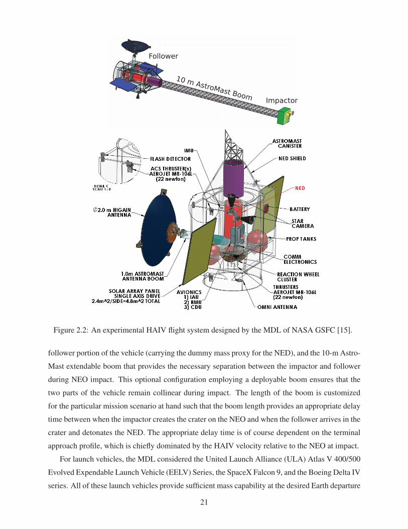
The overall configurationsystem design of an experimental HAIV system is illustrated in Fig 22
This reference HAIV system consists of the leading impactor portion of the vehicle the trailing
20
21
Figure 22 An experimental HAIV flight system designed by the MDL of NASA GSFC [15]
follower portion of the vehicle (carrying the dummy mass proxy for the NED) and the 10-m Astro-
Mast extendable boom that provides the necessary separation between the impactor and follower
during NEO impact This optional configuration employing a deployable boom ensures that the
two parts of the vehicle remain collinear during impact The length of the boom is customized
for the particular mission scenario at hand such that the boom length provides an appropriate delay
time between when the impactor creates the crater on the NEO and when the follower arrives in the
crater and detonates the NED The appropriate delay time is of course dependent on the terminal
approach profile which is chiefly dominated by the HAIV velocity relative to the NEO at impact
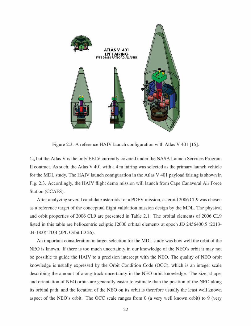
For launch vehicles the MDL considered the United Launch Alliance (ULA) Atlas V 400500
Evolved Expendable Launch Vehicle (EELV) Series the SpaceX Falcon 9 and the Boeing Delta IV
series All of these launch vehicles provide sufficient mass capability at the desired Earth departure
22
Figure 23 A reference HAIV launch configuration with Atlas V 401 [15]
C3 but the Atlas V is the only EELV currently covered under the NASA Launch Services Program
II contract As such the Atlas V 401 with a 4 m fairing was selected as the primary launch vehicle
for the MDL study The HAIV launch configuration in the Atlas V 401 payload fairing is shown in
Fig 23 Accordingly the HAIV flight demo mission will launch from Cape Canaveral Air Force
Station (CCAFS)
After analyzing several candidate asteroids for a PDFV mission asteroid 2006 CL9 was chosen
as a reference target of the conceptual flight validation mission design by the MDL The physical
and orbit properties of 2006 CL9 are presented in Table 21 The orbital elements of 2006 CL9
listed in this table are heliocentric ecliptic J2000 orbital elements at epoch JD 24564005 (2013shy
04-180) TDB (JPL Orbit ID 26)
An important consideration in target selection for the MDL study was how well the orbit of the
NEO is known If there is too much uncertainty in our knowledge of the NEOrsquos orbit it may not
be possible to guide the HAIV to a precision intercept with the NEO The quality of NEO orbit
knowledge is usually expressed by the Orbit Condition Code (OCC) which is an integer scale
describing the amount of along-track uncertainty in the NEO orbit knowledge The size shape
and orientation of NEO orbits are generally easier to estimate than the position of the NEO along
its orbital path and the location of the NEO on its orbit is therefore usually the least well known
aspect of the NEOrsquos orbit The OCC scale ranges from 0 (a very well known orbit) to 9 (very
Table 21 Physical and orbital properties of a reference target (asteroid 2006 CL9) [15]
Parameters Values
Absolute magnitude H 2273
Estimated diameter (wp = 013) 104 m
Estimated diameter (wp = 025) 75 m
Rotation period 0145 plusmn 30 hours
Semi-major axis a 134616 AU
Eccentricity e 023675
Inclination i 293551 deg
Longitude of Ascending Node Ω 139313 deg
Argument of Perihelion ω 994912 deg
Mean Anomaly at Epoch M0 209664 deg
OCC 5
Earth MOID 003978 AU
Table 22 Notional flight validation mission selected for 2006 CL9 [15]
Parameters Values
Earth departure date 2019-08-02
Earth departure C3 1199 km2s2
Flight time to intercept 12141 days
NEO Relative velocity at intercept 115 kms
Approach phase angle 304 deg
Max distance from Earth 036 AU
Max distance from Sun 128 AU
poor orbit knowledge) and NEOs with OCC gt5 are generally considered ldquolostrdquo for the purposes
of locating them in the sky during future observing opportunities
Note that two estimated diameter values for 2006 CL9 are presented in Table 21 based on the
parameter p which is the geometric albedo of the NEO (a measure of how optically reflective its
surface is) The albedos of NEOs vary widely and are very difficult to ascertain from ground based
observations This leads to significant uncertainty in the physical size of most known NEOs The
problem can be summarized as small shiny objects can have the same brightness in the sky as
large dull objects The intrinsic brightness of the NEOs expressed by the absolute magnitude H
is much better constrained (because it is directly observed) than albedo
A reference mission trajectory selected for 2006 CL9 is summarized in Table 22 The refershy
ence trajectory design is based on patched conics with Lambert targeting applied to high-fidelity
ephemerides for the Earth and NEO and therefore no deterministic ΔV is required on the part of
the spacecraft in this initial trajectory design
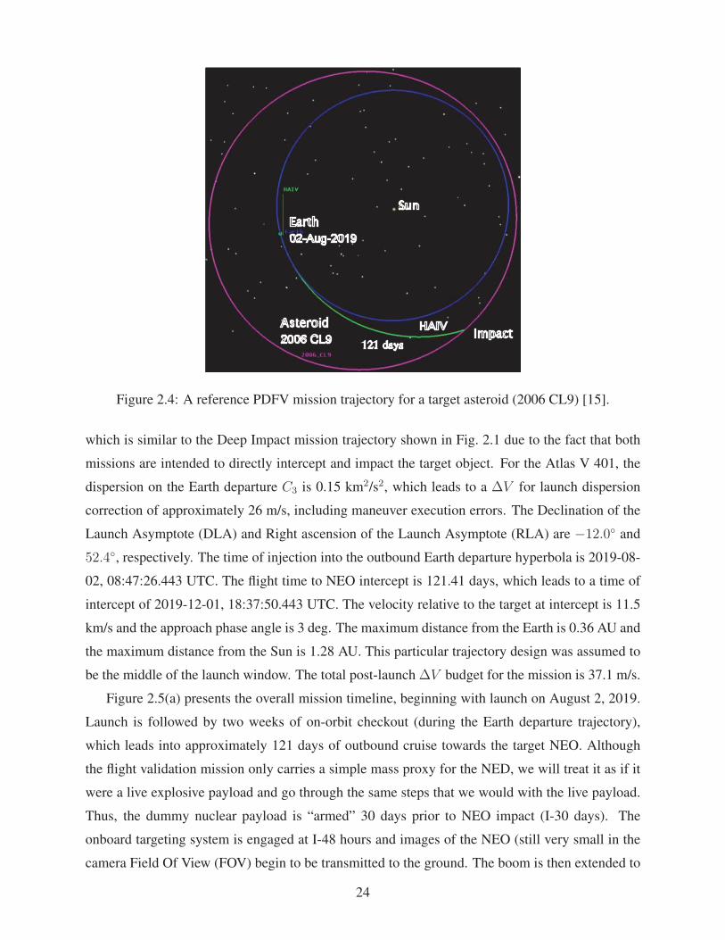
A reference orbital trajectory of a PDFV mission to asteroid 2006 CL9 is shown in Fig 24
23
Figure 24 A reference PDFV mission trajectory for a target asteroid (2006 CL9) [15]
which is similar to the Deep Impact mission trajectory shown in Fig 21 due to the fact that both
missions are intended to directly intercept and impact the target object For the Atlas V 401 the
dispersion on the Earth departure C is 015 km2s23 which leads to a ΔV for launch dispersion
correction of approximately 26 ms including maneuver execution errors The Declination of the
Launch Asymptote (DLA) and Right ascension of the Launch Asymptote (RLA) are minus120 and
524 respectively The time of injection into the outbound Earth departure hyperbola is 2019-08shy
02 084726443 UTC The flight time to NEO intercept is 12141 days which leads to a time of
intercept of 2019-12-01 183750443 UTC The velocity relative to the target at intercept is 115
kms and the approach phase angle is 3 deg The maximum distance from the Earth is 036 AU and
the maximum distance from the Sun is 128 AU This particular trajectory design was assumed to
be the middle of the launch window The total post-launch ΔV budget for the mission is 371 ms
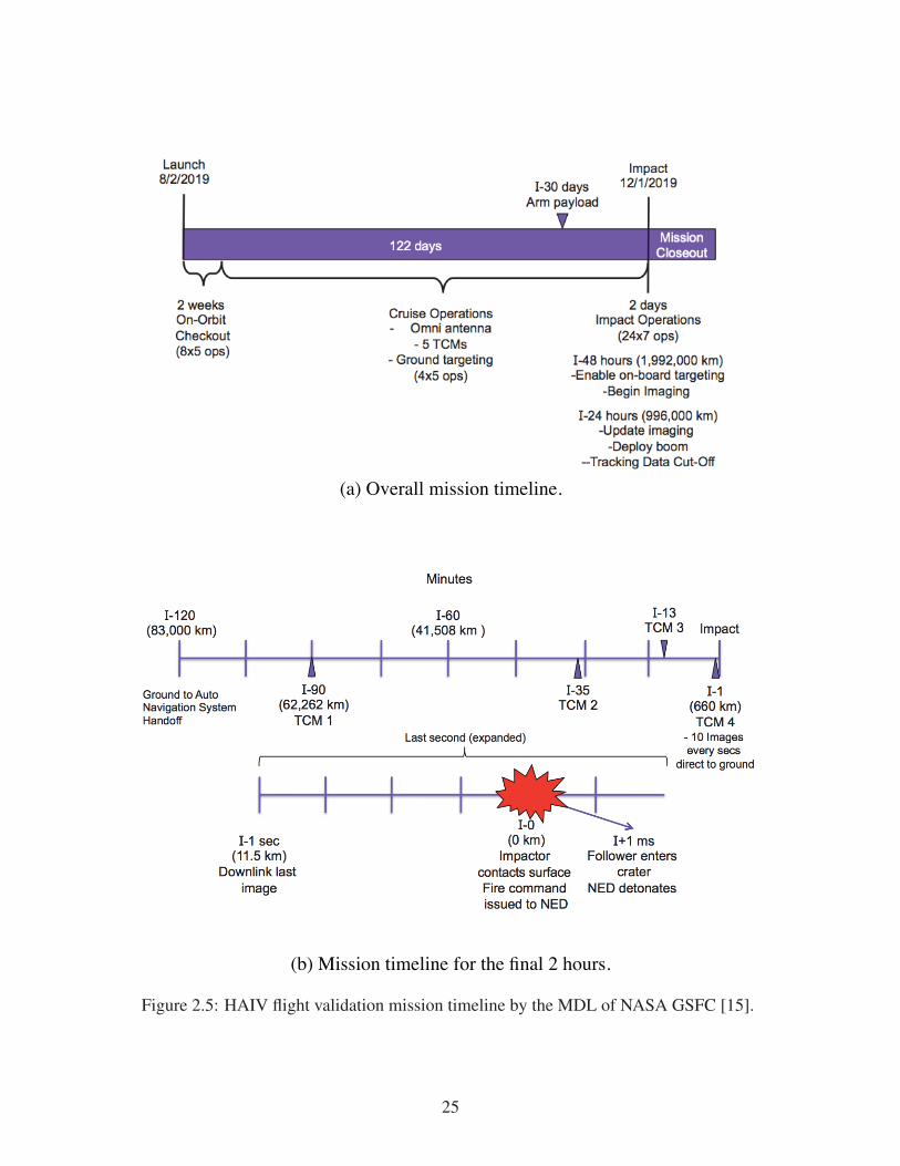
Figure 25(a) presents the overall mission timeline beginning with launch on August 2 2019
Launch is followed by two weeks of on-orbit checkout (during the Earth departure trajectory)
which leads into approximately 121 days of outbound cruise towards the target NEO Although
the flight validation mission only carries a simple mass proxy for the NED we will treat it as if it
were a live explosive payload and go through the same steps that we would with the live payload
Thus the dummy nuclear payload is ldquoarmedrdquo 30 days prior to NEO impact (I-30 days) The
onboard targeting system is engaged at I-48 hours and images of the NEO (still very small in the
camera Field Of View (FOV) begin to be transmitted to the ground The boom is then extended to
24
(
25
(a) Overall mission timeline
(b) Mission timeline for the final 2 hours
Figure 25 HAIV flight validation mission timeline by the MDL of NASA GSFC [15]
deploy the impactor at I-24 hours Figure 25(b) shows the mission timeline for the final 2 hours
At I-2 hours the ground relinquishes control to the space vehicle and the Trajectory Correction
Maneuvers (TCMs) begin At the final 60 seconds before impact the HAIV is 660 km away from
the NEO and is transmitting 10 images per second to the ground with the final image downlinked
at I-1 second At I-0 the impactor contacts the surface of the NEO (creating a shallow crater) and
that event causes the fire command to be issued to the NED mass proxy (which is instrumented
with the same circuitry that would be used with an actual NED) At I+1 millisecond the follower
portion of the vehicle enters the crater and the NED would detonate at this time (due to the fire
command having been issued at the proper time 1 millisecond prior to crater entry)
223 Terminal Guidance Navigation and Control Subsystem
One of key subsystems of the HAIV is the terminal Guidance Navigation and Control (GNC)
subsystem which is briefly described here The MDL performed a complete navigation simulation
of the terminal approach phase beginning at I-2 hours The navigation simulation included a linear
covariance analysis and a Monte Carlo error analysis The navigation simulation utilized a sequenshy
tial Kalman filter with observations derived from the asteroid centroid location in the sensor CCD
(Charge-Coupled Device) The navigation filter is solving for the inertial position and velocity
of the spacecraft with respect to the asteroid The simulation software utilized is the Orbit Deshy
termination Toolbox (ODTBX) which is an advanced mission simulation and analysis tool used
for concept exploration early design phases and rapid design center environments ODTBX is
developed by the Navigation and Mission Design Branch at NASA Goddard Space Flight Center
The software is released publicly under the NASA Open Source Agreement and is available on
SourceForge at httpsourceforgenetprojectsodtbx
The optical navigation sensors modeled in the simulations are based on the Deep Impact misshy
sionrsquos Impactor Targeting Sensor (ITS) which has a Field Of View (FOV) of 06 a focal length
of 2101 mm and a resolution of 1024 times 1024 The navigation relies on identification of the target
body centroid in the sensor field of view The acquisition requirement is to be able to detect a 13th
apparent magnitude object with a signal-to-noise ratio of at least 10 within a 5-second exposure
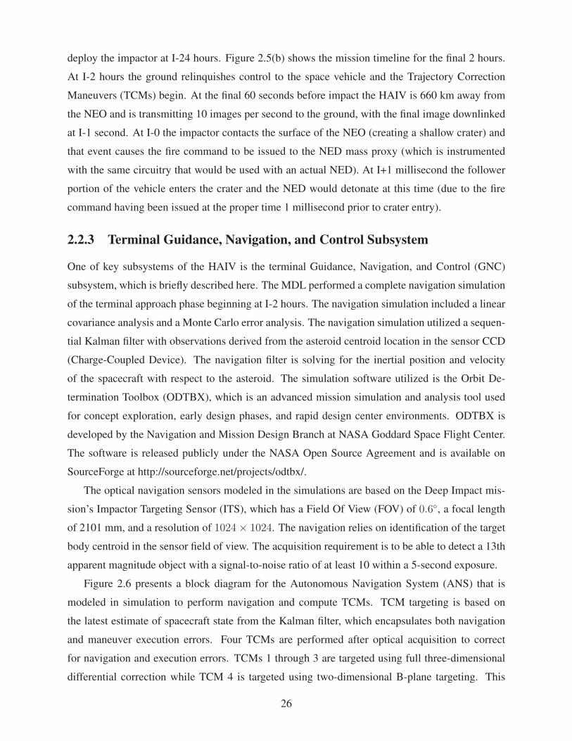
Figure 26 presents a block diagram for the Autonomous Navigation System (ANS) that is
modeled in simulation to perform navigation and compute TCMs TCM targeting is based on
the latest estimate of spacecraft state from the Kalman filter which encapsulates both navigation
and maneuver execution errors Four TCMs are performed after optical acquisition to correct
for navigation and execution errors TCMs 1 through 3 are targeted using full three-dimensional
differential correction while TCM 4 is targeted using two-dimensional B-plane targeting This
26
Navigation Camera
Translation Dynamics
Hydrazine Thrusters
Attitude Control System
Image Processing
[pl ]
Kalman Filter [RV ]
Maneuver Planning
[ V ]
Autonomous Navigation Software
Ground Flight Dynamics
System
Figure 26 Block diagram of the Autonomous Navigation System (ANS) of an experimental HAIV [15]
was found to be the most robust targeting scheme after initial experimentation because the range
between the HAIV and the target NEO is not very observable and that compromises targeting
schemes that rely solely on full three-dimensional position targeting The ground-to-ANS handoff
occurs at Indash2 hours at which time the iquestLJKt dynamics system on the ground provides a frac34QDl state
update to the HAIV and hands over translational control to the ANS The ANS computes and
executes TCMs at Indash90 minutes Indash35 minutes Indash12 minutes and Indash1 minute The ANS was
exercised for our target NEO scenario with a Monte Carlo simulation to characterize performance
in terms of impact accuracy
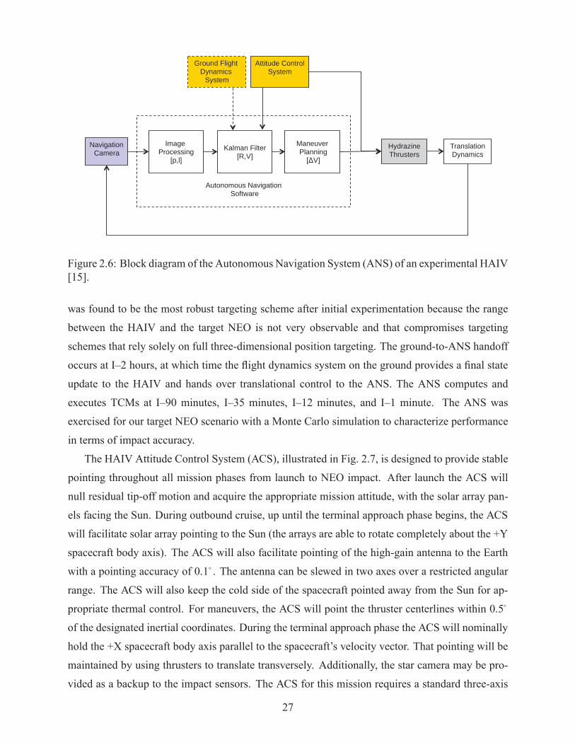
The HAIV Attitude Control System (ACS) illustrated in Fig 27 is designed to provide stable
pointing throughout all mission phases from launch to NEO impact After launch the ACS will
null residual tip-off motion and acquire the appropriate mission attitude with the solar array pan-
els facing the Sun During outbound cruise up until the terminal approach phase begins the ACS
will facilitate solar array pointing to the Sun (the arrays are able to rotate completely about the +Y
spacecraft body axis) The ACS will also facilitate pointing of the high-gain antenna to the Earth
with a pointing accuracy of 01ƕ The antenna can be slewed in two axes over a restricted angular
range The ACS will also keep the cold side of the spacecraft pointed away from the Sun for ap-
propriate thermal control For maneuvers the ACS will point the thruster centerlines within 05ƕ
of the designated inertial coordinates During the terminal approach phase the ACS will nominally
hold the +X spacecraft body axis parallel to the spacecraftrsquos velocity vector That pointing will be
maintained by using thrusters to translate transversely Additionally the star camera may be pro-
vided as a backup to the impact sensors The ACS for this mission requires a standard three-axis
27
Figure 27 Block diagram of the Attitude Control System (ACS) of an experimental HAIV [15]
stabilized system The attitude sensors include two star cameras and an inertial reference unit (gyshy
ros and possibly an accelerometer package) While two camera heads are baselined in the design
the data processing unit can accommodate up to four camera heads if needed The attitude actuashy
tors include four reaction wheels arranged in a pyramid to provide mutual redundancy along with
hydrazine thrusters The following attitude control modes are defined for this mission acquisition
cruise terminal phase and safe hold The ACS will be operating continuously using the reaction
wheels and the attitude control thrusters will be used at discrete times for momentum unloading
The attitude control thrusters may also be needed during any ldquoturn-and-burnrdquo maneuvers During
the terminal phase the ACS software will provide the inertial-to-body frame quaternion to the
ANS
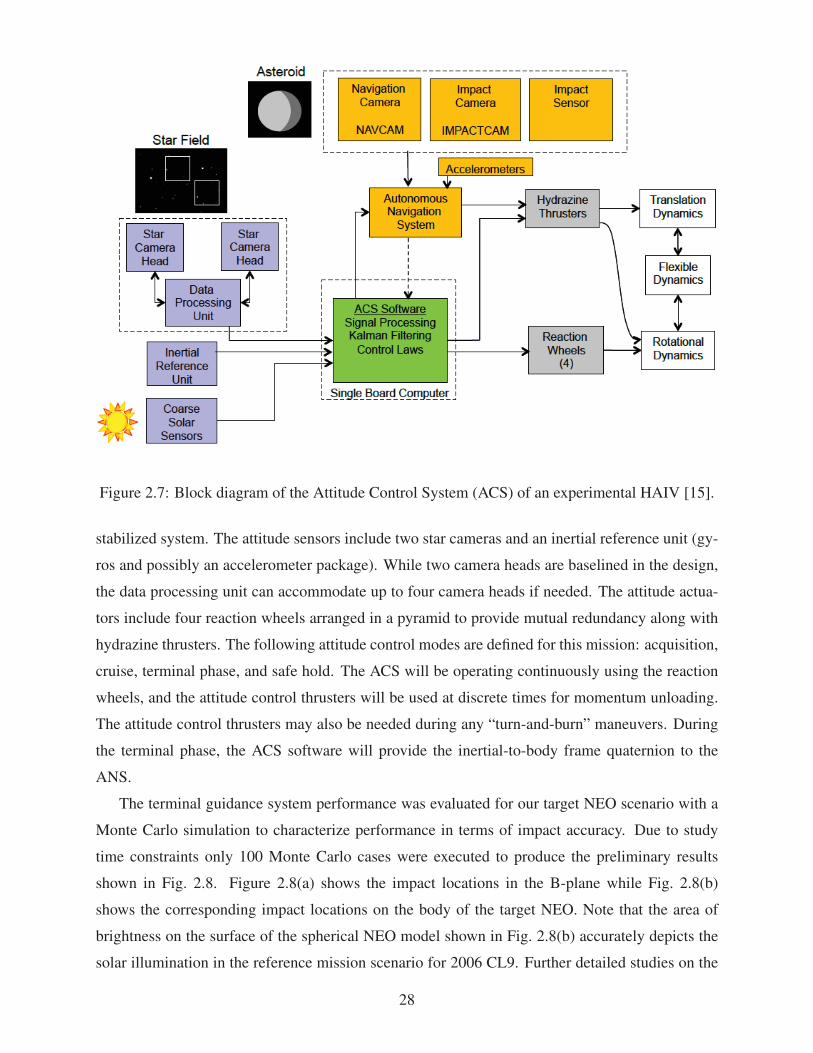
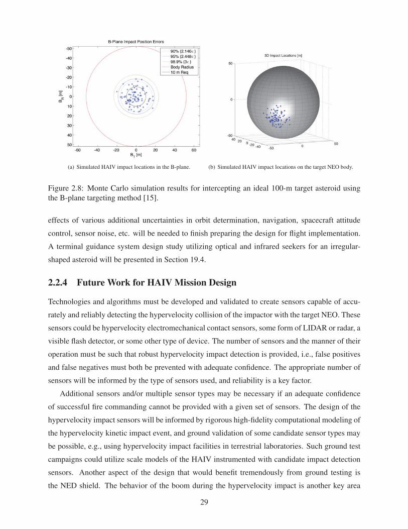
The terminal guidance system performance was evaluated for our target NEO scenario with a
Monte Carlo simulation to characterize performance in terms of impact accuracy Due to study
time constraints only 100 Monte Carlo cases were executed to produce the preliminary results
shown in Fig 28 Figure 28(a) shows the impact locations in the B-plane while Fig 28(b)
shows the corresponding impact locations on the body of the target NEO Note that the area of
brightness on the surface of the spherical NEO model shown in Fig 28(b) accurately depicts the
solar illumination in the reference mission scenario for 2006 CL9 Further detailed studies on the
28
29
Figure 28 Monte Carlo simulation results for intercepting an ideal 100-m target asteroid using
the B-plane targeting method [15]
(a) Simulated HAIV impact locations in the B-plane (b) Simulated HAIV impact locations on the target NEO body
effects of various additional uncertainties in orbit determination navigation spacecraft attitude
control sensor noise etc will be needed to finish preparing the design for flight implementation
A terminal guidance system design study utilizing optical and infrared seekers for an irregular-
shaped asteroid will be presented in Section 194
224 Future Work for HAIV Mission Design
Technologies and algorithms must be developed and validated to create sensors capable of accushy
rately and reliably detecting the hypervelocity collision of the impactor with the target NEO These
sensors could be hypervelocity electromechanical contact sensors some form of LIDAR or radar a
visible flash detector or some other type of device The number of sensors and the manner of their
operation must be such that robust hypervelocity impact detection is provided ie false positives
and false negatives must both be prevented with adequate confidence The appropriate number of
sensors will be informed by the type of sensors used and reliability is a key factor
Additional sensors andor multiple sensor types may be necessary if an adequate confidence
of successful fire commanding cannot be provided with a given set of sensors The design of the
hypervelocity impact sensors will be informed by rigorous high-fidelity computational modeling of
the hypervelocity kinetic impact event and ground validation of some candidate sensor types may
be possible eg using hypervelocity impact facilities in terrestrial laboratories Such ground test
campaigns could utilize scale models of the HAIV instrumented with candidate impact detection
sensors Another aspect of the design that would benefit tremendously from ground testing is
the NED shield The behavior of the boom during the hypervelocity impact is another key area
that must be studied through both high-fidelity computer simulations and possibly ground testing
We must be certain that the size shape and materials used to construct the boom fail during the
hypervelocity impact in a manner that does not threaten the NED payload the impact sensors
or the production and reception of the NED fire command signal At the same time during the
process of advancing the design for actual implementation it will be necessary to further assess
the feasibility advantages and disadvantages of having the impactor and follower be physically
separated free-flying vehicles rather than connected by a boom
Another key area of analysis is the final approach timeline The results presented herein demonshy
strate that the final approach timeline depends on the target NEO diameter and albedo as well as
the approach phase angle relative to the NEO and the relative velocity at impact Developing parashy
metric models for the approach timeline as a function of these and other key driving parameters will
facilitate refinement of the onboard optical systems to ensure acquisition of the target sufficiently
far in advance of the impact for the ANS to be able to operate robustly and achieve a precise and
accurate impact with high confidence We can also adjust our trajectory optimization algorithms
to attempt to minimize the intercept velocity within the constraints that the crater excavated on the
NEO is of sufficient depth and that the additional maneuver required for intercept velocity control
is within our available ΔV budget
One of the driving requirements of the HAIV system is the requirement that the flight experishy
ment must be able to be fully validated in ground post-processing of the HAIV telemetry While
this requirement actually leads to a robust design it would clearly be beneficial to have an observer
spacecraft present near the target NEO before and after the impact to more directly observe and
characterize the HAIV performance As such subsequent to the MDL study we developed new
algorithms to perform trajectory scans that identify mission opportunities in which an observer
and HAIV spacecraft can be both transported to the NEO (at different times) for low ΔV The
results of these new mission opportunity searches may reveal affordable options for having both
an observer and a HAIV in the mission simultaneously Another alternative worth considering is
having the HAIV deploy a free-flying observer that could also serve as calibration target during
the cruise to the NEO The difficulty with this option is that the deployed free-flying system would
need to be capable of high bandwidth communications with Earth and would therefore probably be
so large that the it cannot reasonably treated as a small deployable add-on in that case we return to
the aforementioned alternative of deploying a fully capable observer as a separate spacecraft The
final variation on this option is to have another entity supply the observer spacecraft since it is fully
decoupled from the HAIV For example NASA could build deploy and operate the HAIV while
another agency eg ESA could build deploy and operate the observer spacecraft This scenario
is advantageous from the perspective of addressing the international nature of planetary defense
30
The MDL study identified other areas of beneficial forward work some of which have been
addressed during our NIAC phase 2 work These include improvement of ANS performance and
robustness for NEO targeting accuracy and maneuver magnitude management using the GNC
algorithms to process synthetic imagery for realistic cases including irregularly shaped rotating
NEOs of various sizes and assessment of the effects of NEO density on the cratering performance
of the kinetic impactor portion of the HAIV
225 Summary
This section has presented the results of a NASAGoddard Space Flight Center (GSFC) Mission
Design Lab (MDL) study for the conceptual design of the HAIV flight validation mission as part
of our NIAC Phase 2 study [15] The MDL study provided a feasible and detailed conceptual
design for the HAIV flight validation mission and identified a number of key topics for further
research These research topics include high-fidelity computational modeling of hypervelocity
impact physics detailed development of advanced GNC algorithms for precision hypervelocity
intercept of small (50 to 150 m size) NEOs and design and development of test plans for robust
hypervelocity impact sensors In our subsequent research we continued to refine deepen expand
and advance the design of the HAIV system and its flight validation mission
The estimated cost of an experimental HAIV flight demonstration mission described in this secshy
tion is approximately $530M including the launch vehicle [15] An approximate cost of $150M
is assumed for the notional launch vehicle which is the Atlas V 401 The cost estimate is compreshy
hensive and includes the complete design construction integration and testing of the spacecraft
itself launch vehicle integration and test project management mission operations ground system
systems integration and test education and public outreach and project reserves More details of
the HAIV flight validation mission design by the MDL of NASA GSFC can be found in [15]
When a hazardous NEO on a collision course with Earth is discovered we will not have the
luxury of designing testing and refining our systems and plans We will need to be prepared to
take effective action on relatively short notice with a high probability of succeeding on the first
try because we may not have a second chance That level of preparedness can only be achieved
through proper design and testing of systems so that we are comfortable with carrying out planetary
defense test and practice missions before we need to deploy such a mission in response to an actual
threat
23 Target Selection for the PDFV Mission
In [15 28] a simple direct intercept mission trajectory as illustrated in Fig 24 similar to the
Deep Impact mission trajectory shown in Fig 21 was found to be the best option for the PDFV
31
Table 23 Target selection criteria for the Don Quijote mission study [29]
Orbit Characteristics Preferred Range
Rendezvous ΔV lt 7 kms
Orbit type Amor
MOID large and increasing
Orbit accuracy well determined orbits
Physical Characteristics Preferred Range
Size lt 800 m
Density sim13 gcm3
Absolute magnitude 204 - 196
Shape not irregular
Taxonomic type C-type
Rotation period lt 20 hours
Binarity not binary
mission The direct intercept mission has the largest number of feasible candidate target asteroids
requires a minimal total post-launch ΔV and is a representative of the most probable worst-case
asteroid mitigation mission scenario with short warning time More advanced missions which
enable an observer spacecraft to arrive at the asteroid prior to the main spacecraft impact have
also been analyzed in [28] The results generally show that allowing the impactor spacecraft to
perform multiple gravity assists lowers the total required ΔV for each mission considered as well
as increases the impactor arrival velocity Several feasible gravity-assist rendezvous missions are
presented in [28] There are several possible target asteroids which require a total ΔV of 15 kms
or less with the most efficient combined rendezvousimpact mission requiring only approximately
600 ms of ΔV
231 Reference Targets of the Don Quijote Mission Study
Although the Don Quijote mission was never realized and launched by ESA it is useful to review
the target selection process once considered for the Don Quijote mission [29ndash31] Its target selecshy
tion criteria were based on a set of NEO characteristics defined by ESArsquos NEOMAP summarized
in Table 23 A preliminary selection resulted in the asteroids 2002 AT4 and 1989 ML As seen in
Table 24 asteroid 2002 AT4 is roughly half the size of 1989 ML but intercepting it requires more
ΔV
232 Target Selection Problem Formulation
A comparison of NEA orbit families is shown in Fig 29 For a PDFV mission NEAs in the Atira
and Amor orbit groups are preferred as target candidates NEAs in these groups all have perihelion
32
Table 24 Properties of candidate targets formerly considered for the Don Quijote mission study
[29]
2002 AT4 1989 ML
Orbital period (yrs) 2549 1463
e 0447 0137
i (deg) 15 44
ΔV (kms) 658 446
Orbit type Amor Amor
MOID large large
Absolute magnitude 2096 1935
Taxonomic type D-type E-type
Diameter (m) 380 800
Rotational period (hrs) 6 19
Sun
Earth Atira
Amor
Apollo
Aten
33
Figure 29 Typical orbits of Amor Apollo Aten and Atira asteroids
distances lt 13 AU and many of them also cross the Earthrsquos orbit at some point The proximity of
NEA orbits to Earthrsquos orbit means that the ΔV required for intercept is usually small As such we
expect that a number of NEAs will prove to be viable candidates for a NEA deflectiondisruption
flight validation mission Apollo and Aten NEA orbits cross Earthrsquos orbit and in some cases this
leads to lower mission ΔV requirements as compared to Atiras or Amors On the other hand this
same fact means that any significant perturbation to the NEArsquos orbit could cause it to impact the
Earth later Such unintended consequences must not occur This is the reason why ESA considered
asteroids 2002 AT4 and 1989 ML from the Amor group for the Don Quijote mission [29ndash31]
To preclude the possibility of inadvertently perturbing a previously harmless NEA onto an
Earth collision course only Atira and Amor NEAs are considered for a PDFV mission in [15 28]
The Amor asteroid group is characterized by asteroids that approach the Earth but do not actually
cross its orbit By definition the perihelion distances of these asteroids lie between 1017 and
13 AU As of July 21 2012 there were 3398 Amor and Atira asteroids listed in NASArsquos NEO
Program database Only 10 of those are Atira asteroids because their orbits are entirely inside
Earthrsquos orbit and we currently have no space-based NEO survey it is very difficult to discover
Atiras Amor asteroid orbits are entirely outside of the Earthrsquos orbit Because the orbits of Atiras
and Amors are entirely interior or exterior to Earthrsquos orbit respectively disturbances to the orbits
of those asteroids due to human activity are not likely to cause those asteroids to move onto Earth-
impacting orbits after the PDFV mission
A mission design software tool capable of performing advanced mission analysis for thousands
of potential target asteroids is described in [28] Due to the large number of design parameters in
this type of mission design an exhaustive search of all 3398 asteroids would be impractical Conshy
sequently all mission design computation is performed using an evolutionary genetic algorithm
in [28] A combination of evolutionary algorithms modular mission design software and modern
GPUs (Graphics Processing Units) allows computationally efficient design of multiple possible
mission architectures for thousands of possible target asteroids
The first constraint imposed ensures that the HAIV will be able to communicate with Earth
ground stations during the final impact phase of the mission This is achieved by penalizing any
mission where the impact would occur on the opposite side of the sun from the Earth The exact
angle limitations for the impact Earth-Asteroid angle are the angle must be lt175 from the Earth
and gt185 from the Earth as illustrated in Fig 210 The second main constraint is a guidance
and navigation constraint such that the impactor approaches from the sunward side of the asteroid
This constraint ensures proper lighting conditions for the terminal guidance phase of the mission
The purpose of a PDFV mission is to demonstrate the feasibility of the HAIV system for the
purpose of planetary defense The HAIV is designed for the hypervelocity impacts that are likely
34
Excluded
Figure 210 Illustration of the Earth-Sun-Asteroid line-of-sight communication angle excludedfor the PDFV mission [28]
to be required by planetary defense missions executed with short warning time Therefore the
PDFV mission must have a minimum impact velocity of 5 kms Due to anticipated technological
limitations impact velocities over 30 kms are penalized as well However it should be noted that
none of the missions analyzed have had an impact velocity above 30 kms meaning the HAIV
impactor never has to decrease its approach velocity All other major mission constraints are
provided in Table 25 The exact penalty functions are also discussed in [28] It is worth noting
that limitations on NEA orbit group and absolute magnitude reduce the number of asteroids that
must be searched from approximately 3500 to 1500
233 Direct Intercept PDFV Mission
35
Earth
Sun
MissionFeasible
MissionFeasible
For the direct intercept mission an appropriate launch vehicle is used to inject the HAIV into
an interplanetary orbit that directly intercepts the target asteroid This is the simplest mission
type analyzed in [28] with only two variables to optimize (launch date and time-of-flight to the
asteroid) and yields the largest number of feasible target asteroids For direct intercept missions a
relatively low C limit of 125 km2s 2 3 is used By limiting missions to low C3 it may be possible
to use a less capable (and therefore less expensive) launch vehicle than for missions that include
both an impactor and rendezvous (observer) spacecraft
Table 25 The PDFV mission constraints [28]
Parameters Values
Asteroid types Amor Atira
Earliest launch date 1-Jan-2018
Latest launch date 31-Dec-2022
Minimum impact velocity 5 kms
Maximum impact velocity 30 kms
H magnitude range 2075-2362
Communication LOS constraints lt175 and gt185
Impact angle constraint penalized if approach isnrsquot from the sunward side
Impactor limitations For dual missions the impact must occur
after rendezvous SC arrival
Maximum departure C3 125 km2s2 for single SC mission
30 km2s2 for dual SC missions
Table 26 Top 3 target asteroid candidates for a simple direct intercept PDFV mission [28]
Asteroid 2006 CL9 2009 QO5 2004 BW18
a (AU) 135 159 137
e 024 024 025
Diameter (m) 104 105 97
Departure C3 (km2s2) 1199 1250 1249
SC ΔV (kms) 00 00 00
LOS angle) 349 349 333
Sun phase angle 3 28 34
Departure date 2-Aug-2019 27-Mar-2019 7-Apr-2019
TOF (days) 12141 12438 26845
OCC 5 1 5
Impact velocity (kms) 1153 922 657
With the low C3 limit hundreds of potential target asteroids were found during the search
in [28] These asteroid require no ΔV from the HAIV impactor other than minor trajectory corshy
rections during the terminal guidance phase of the mission The results presented in Table 26
represent the top 3 candidate asteroids These asteroids were chosen because their orbits are fairly
well known (or future observations of them will be possible prior to the mission launch dates)
Another consideration in the target search is how well the orbit of the target NEO is known
If there is too much uncertainty in our knowledge of the NEOrsquos orbit it may not be possible to
guide the HAIV to a precision intercept with the NEO The quality of NEO orbit knowledge is
usually expressed by the Orbit Condition Code (OCC) which is an integer scale describing the
amount of along-track uncertainty in the NEO orbit The OCC is also known as the Minor Planet
Center (MPC) ldquoUrdquo parameter (httpwwwminorplanetcenternetiauinfo) The size shape and
36
orientation of NEO orbits are generally easier to estimate than the position of the NEO along its
orbital path and the location of the NEO on its orbit is therefore usually the least well known
aspect of the NEOrsquos orbit The OCC scale ranges from 0 (a very well known orbit) to 9 (very
poor orbit knowledge) and NEOs with OCC gt5 are generally considered ldquolostrdquo for the purposes
of locating them in the sky during future observing opportunities [15]
A filter of OCC smaller than 5 is considered in [15 28] for NEO target search The trajectory
scans were applied to Amor and Atira NEOs with estimated diameter near 100 m and OCC smaller
than 5 The trajectory scan constraints included Earth departure characteristic energy C3 lt125
km2s2 Earth departure date between 2018 and 2020 Sun-Spacecraft-Earth (SSE) angle at the time
of intercept gt3 and sun phase angle at intercept lt90 The SSE angle is measured between the
vector that points from the spacecraft to the Sun and the vector that points from the spacecraft to the
Earth If the SSE angle is too small then the Sun may interfere with communications between the
spacecraft and Earth and we require a good communications link with the spacecraft especially
at the time of NEO intercept in order to collect the telemetry needed to confirm the success of the
flight experiment [15]
The sun phase angle at intercept is measured between the velocity vector of the spacecraft
relative to the NEO and the heliocentric position vector of the NEO at the time of intercept A
phase angle of zero places the spacecraft directly between the Sun and the NEO at the time of
intercept while a phase angle of 90 means that the spacecraft approaches the NEO orthogonal
to the NEO-Sun line Designing the trajectory so that a small value of the phase angle obtains
provides a situation in which the Sun is naturally illuminating the full face of the NEO or nearly
so from the spacecraftrsquos perspective during terminal approach which is highly advantageous for
optical acquisition of the NEO with the spacecraftrsquos onboard cameras and especially important for
small NEOs that are optically faint even under such ideal circumstances
After analyzing the trajectory scan results the asteroid 2006 CL9 was selected as the notional
target for the conceptual flight validation mission in [15 28] Another factor in the selection of
2006 CL9 is that while its OCC value of 5 would present navigation challenges for the PDFV
mission there may be opportunities to gather more ground-based observations of this NEA within
the next couple of years which may improve our knowledge of its orbit and thus reduce the OCC
It happens that this NEA meets the criteria for NASArsquos Near-Earth Object Human Space Flight
Accessible Targets Study (NHATS) [32] and the next upcoming observing opportunity is among
the NHATS data published for the NEAs
A reference PDFV mission trajectory for asteroid 2006 CL9 has been shown previously in
Fig 24 which is similar to the Deep Impact mission trajectory shown in Fig 21 due to the fact
37
Figure 211 International efforts in preparing for a planetary defense mission Image courtesy of
Lindley Johnson at NASANEOO
that both missions are intended to directly intercept and impact the target object More detailed
description of this reference PDFV mission can be found in [15] Advanced PDFV mission design
for accommodating both rendezvous spacecraft and direct intercept spacecraft is also presented
in [28] A complex orbital trajectory optimization algorithm developed in [33 34] for combined
multiple gravity-assist maneuvers and impulsive ΔV maneuvers is utilized in [28]
24 Recommendations for Planetary Defense
With a mandate from the UN Committee on the Peaceful Uses of Outer Space (COPUOS) the
Space Mission Planning and Advisory Group (SMPAG) has been established in 2013 to coordinate
a global response should a threatening asteroid be found heading toward Earth as illustrated in
Fig 211 The NEO Observation (NEOO) Program Office of NASA has been coordinating all
efforts related to NEO survey detection and impact warning
However no agency of the US federal government has been officially designated for planshy
ning andor preparing for planetary defense actions prior to detection of a real impact threat (the
warning time for which as noted previously may be quite short) Therefore we recommend that a
US government agency be formally designated by the Congress for the coordination of all RampD
activities of preparing for all planetary defense options prior to detecting any impact threat
38
y
1 day
Interplanetary Hypervelocity Asteroid
Intercept Vehicle (the only option)
Nuclear Standoff Kinetic Impactors Gravity Tractors
etc (many options)
12
2012 DA14
DeflectionFragmentation
Chelyabinsk Meteor
2006 NEO Report by NASA 2010 NEO Report by NRC
(2005 NEPW Report by NRC)
Figure 212 A summary of various mitigation options for planetary defense
If we have sufficient warning time (gt10 years) then various options including kinetic imshy
pactors gravity tractors and nuclear standoff explosions can be employed for a non-destructive
deflection mission For the more probable impact threat scenario in which the warning time is less
than 5 years a disruptiondispersion mission employing nuclear explosions is likely to become
the only option (other than evacuation of the area affected by the impact on Earth assuming the
impacting NEO is not large enough to be globally catastrophic) Various mitigation options for a
wide range of warning times (1 week to 20 years) are summarized in Figs 212 and 213
The mission effectiveness of the proposed HAIV system can be further enhanced by exploiting
an asteroid warning system which is being developed at the University of Hawaii with $5 milshy
lion funding from NASA Once this system called the ATLAS (Asteroid Terrestrial-impact Last
Alert System) becomes fully operational in early 2016 it is expected that it will offer a one-week
warning for a 45-m asteroid and three weeks for a 140-m asteroid Provided that such one-week
warning from the ATLAS can be assured a target asteroid gt45 m in size can be intercepted and
disrupted far outside of Earthrsquos gravitational sphere of influence and consequently avoid a potenshy
tially troublesome suborbital intercept It is emphasized that a suborbital intercept may become
inevitable for situations with ultra-short warning times of only 1 to 24 hrs (to be further discussed
in Chapter 5)
39
Asteroid Deflection Research Center
Early Warning (gt 10 yrs) ldquoBuild and Launchrdquo (Deflection)
gt 2 yrs ldquoBuild and Launchrdquo (Deflection or Disruption)
lt 1 yr ldquoReady to Launchrdquo (Disruption)
NASA Innovative Advanced Concepts
ATLAS Last Alert 3-week (gt 140 m) ldquoReady to Launchrdquo (Interplanetary)1-week (gt 45 m)
ATLAS project head Dr John Tonry with a conceptual drawing for an ATLAS ldquoReady to Launchrdquotelescope The project would use two of these 20-inch telescopes Credit 1 day ndash 1 wkUHIfA (Suborbital Intercept) IPBMHAIV
Figure 213 Applicability of the HAIV mission concept to various mission scenarios
Most NEO science missions required at least several years in some cases 5 to 6 years or more
for mission concept development and spacecraft construction prior to launch It is also important to
note that quite a few of these missions originally targeted different asteroids or comets than those
that were actually visited This is because the mission development schedules slipped and launch
windows for particular asteroids or comets were missed Additionally several of these missions
experienced hardware or software failures or glitches that compromised the completion of mission
objectives None of those things would be tolerable for a planetary defense mission aimed at
deflecting or disrupting an incoming NEO especially with relatively little advance warning Thus
while the successful scientific missions that have been sent to asteroids and comets thus far have
certainly provided future planetary defense missions with good heritage on which to build we are
clearly not ready to respond reliably to a threatening NEO scenario
It is also important to note that most of these missions visited asteroids or comets that range
in size from several kilometers to several tens of kilometers Furthermore the flyby distances
ranged from several tens of kilometers to several thousand kilometers The sole exception to this
is the Deep Impact mission which succeeded in delivering an impactor to the target in 2007
However the mission was aided by the fact that comet 9PTempel 1 is 76 times 49 km in size and
therefore provided a relatively large target to track and intercept The Deep Impact mission was
not intended to be a PDFV mission For planetary defense missions requiring NEO intercept the
requirements will be far more stringent NEO targets with diameters as small as several tens to
hundreds of meters will have to be reliably tracked and intercepted at hypervelocity speeds with
impact occurring within mere meters of the targeted point on the NEOrsquos surface This will require
40
significant evolution of the autonomous guidance and control technology currently available for
science missions to NEOs
Furthermore none of the potential planetary defense mission payloads (eg kinetic impactors
nuclear explosives) to deflect or disrupt NEOs have ever been tested on NEOs in the space environshy
ment Significant work is therefore required to appropriately characterize the capabilities of those
payloads particularly the ways in which they physically couple with NEOs to transfer energy or
alter momentum and ensure robust operations during an actual emergency scenario
With regard to the need for planetary defense spacecraft system testing it is important to note
that there is currently no solicitation for planetary defense flight validation mission proposals Such
missions are necessarily similar in cost to science missions (eg Discovery or New Frontiers) yet
there is no established mechanism for funding planetary defense flight validation missions So
there is a need for planetary defense flight validation mission funding It is worth pointing out that
such missions will naturally by their intrinsic nature return significant amounts of science data
even though they are not primarily science missions
Finally the very nature of the HAIV design (and the motivation for its design) underscores the
need for a dedicated space-based NEO survey telescope located far from Earthrsquos vicinity Such a
telescope would be an affordable and cross-cutting system that simultaneously serves the planetary
defense science and exploration communities Completing the NEO population survey as soon
as possible is the best way to maximize the amount of warning time available to us should we
find a NEO on an Earth-impacting trajectory That cannot be done using Earth-based telescopes
and such telescopes will always be blind to the sunward direction (from which the Chelyabinsk
impactor approached) a space-based NEO survey will not have the same blind spot Although we
are designing the HAIV to address short warning time situations because they are the most stressing
cases and there will always be a risk of such a case occurring we want to emphasize that doing our
best to avoid short warning time scenarios by deploying a space-based NEO survey telescope is the
most prudent course of action Unfortunately as with planetary defense flight validation missions
the NEO survey telescope cannot seem to find a funding source within NASA Therefore we
recommend that NASA make the funding of a dedicated space-based NEO survey telescope a top
priority followed by funding for planetary defense flight validation missions
In summary it is time to initiate a planetary defense flight validation program mandated by
the Congress for demonstrating validating and refining planetary defense technologies in space
so that we will be properly prepared to respond effectively when a near-Earth object (NEO) on a
collision course with Earth is discovered It will require at least 5 years of further development
and space flight validation testing before operational planetary defense technologies could be
41
employed in a real short warning time situation Now is the time to initiate such preparations
Waiting until a threatening NEO is discovered will be far far too late In addition it is time to
build and launch a dedicated space-based NEO survey telescope stationed far from Earthrsquos vicinity
Such a system will be a key asset that simultaneously benefits planetary defense fundamental solar
system science and space exploration
42
Chapter 3
Terminal Intercept Guidance with Optical and Infrared Seekers
The terminal intercept GNC (Guidance Navigation and Control) is one of the key enabling techshy
nology areas critical for a successful HAIV mission On July 4 2005 the performance of a closed-
loop terminal guidance system employing strapdown optical navigation was flight demonstrated
by NASArsquos Deep Impact mission for impacting a large 5-km comet at an impact speed of 10
kms [25ndash27] However a reliable and accurate intercept of a smaller (50 to 150 m) target NEO
with an impact speed of 30 kms in worst-case circumstances will be a technically challenging
problem To study the feasibility of a HAIV mission for intercepting a small NEO a closed-loop
terminal guidance simulator has been developed by utilizing a polyhedron shape model of asteroid
433 Eros as well as GPU (Graphics Processing Units) computation This chapter describes a new
terminal guidance system architecture employing a strapdown IR (Infrared) seeker to be employed
for a HAIV mission [35ndash39]
31 Introduction
As was illustrated in Fig 15 of Chapter 1 the HAIV mission will end with a terminal intercept
guidance phase during which corrective TCMs (Trajectory Correction Maneuvers) are executed
to compensate for errors in orbital navigation toward the target asteroid The terminal intercept
guidance phase begins some time after the on-board sensors acquire the target For a small (50
m) target asteroid the terminal phase may begin 2 hours prior to intercept while the Deep Impact
mission initiated its terminal guidance 24 hours prior to its final impact with a larger (5 km) comet
Orbital navigation during a terminal phase of the intercept mission will have to be autonomous
as computing and commanding accelerations via a communications link with Earth will be too
time-consuming The interceptor must be able to issue autonomous guidance commands based
solely upon on-board measurements Various options for on-board GNC measurements as well
43
44
Figure 31 Two-dimensional geometry illustration of the terminal intercept guidance problem
[35 36]
as terminal guidance algorithms are discussed in [40 41] The conventional seekers for tactical
missiles or interceptors include optical laser IR and radar seekers [42] There are two types of
seekers employed for a terminal phase of tactical missiles or interceptors They are strapdown
(or body-fixed) seekers and gimbaled seekers The strapdown seekers are directly attached to the
vehicle and their measurements of the target information are relative to the body-fixed coordinate
system The field-of-view (FOV) limitations of such strapdown seekers can be avoided by using
gimbaled seekers which can directly measure the line-of-sight (LOS) angle and the LOS rate
of a target body The seekers are also categorized by semiactive (or passive) and active seekers
depending on the location of their signal sources [42]
Traditional terminal guidance algorithms often require continuous (proportional or throttleable)
accelerations However most divert thrusters are not throttleable ie they are on-off thrusters
The classical proportional navigation (PN) guidance scheme and its numerous variations [42] are
certainly applicable to the terminal intercept guidance of an asteroid impactor
The practicality of a pulsed PN guidance algorithm applied to the asteroid intercept problem has
been investigated in [35 36] The geometry of a terminal intercept guidance problem is illustrated
in Fig 31 The reader is referred to [35 36 42] for detailed discussions of the terminal intercept
guidance problem as illustrated in Fig 31 and an illustrative example of the pulsed PN guidance
law applied to an ideal asteroid intercept problem is briefly described herein
A fictitious 300-m asteroid is assumed to be in a circular orbit with a radius of one astronomical
unit An interceptor with closing velocity of 104 kms is displaced 350 km out radially It is
displaced 24 hours travel time ahead of the target in the tangential direction In the absence of
guidance commands the assumed initial conditions will result in a miss distance of 8829 km A
1000-kg interceptor with two 10-N on-off thrusters is assumed Simulation results summarized
in Figs 32 and 33 indicate that the pulsed PN guidance system performed well for a reference
terminal guidance problem investigated in [35 36]
The effectiveness of a predictive guidance scheme based on orbital perturbation theory has
also been examined in [35 36] Predictive guidance law calculates impulsive velocity corrections
at pre-determined times to eliminate the final miss distance Advanced terminal intercept guidance
algorithms developed in [43 44] can also be employed for the HAIV mission The use of both
optical and IR seekers have been further studied for the HAIV mission in [37ndash39]
This chapter describes the preliminary development of a GPU-based optical navigation and
guidance system simulator utilizing a polyhedron shape model of asteroid scaled 433 Eros shown in
Fig 34 Data for this polyhedron shape model has been obtained from the NEAR collected shape
database [4546] Scaling this model by a factor of 333 generates a reference asteroid model having
a 50-m diameter Adding lighting effects to the asteroid model illuminates the asteroid figure and
create realistic simulated camera images as can be seen in Fig 35 From this lit target the centershy
of-brightness (COB) of the figure will be determined for the guidance and navigation purposes The
COB will be calculated from light intensity of each camera pixel The intercept is accomplished
by estimating the LOS and LOS rate relative to the COB then using this information in the desired
guidance scheme Along with optical image processing the plausibility of an asteroid impact
for a two-body HAIV separating at 60 seconds before the final impact occurs has been studied
in [37 38] This separation concept is taken from the Deep Impact mission where the impactor
separated from the flyby spacecraft at a relative speed of approximately 36 cms Once the fore
and aft body separation occurs at 60 seconds before the final impact for the HAIV mission no
additional control effort is applied
In this chapter a new terminal guidance system architecture for the HAIV mission is also
described Most previous terminal guidance system studies for an asteroid intercept problem
[35 40 41] have considered mainly optical cameras due to their cost-effective nature and acceptshy
able target tracking performance as was demonstrated by Deep Impact mission [25ndash27] However
similar to the case of Raytheonrsquos Exoatmospheric Kill Vehicle (EKV) an IR seeker may need to
be considered for the HAIV mission requiring reliable and accurate target tracking and intercept
of small asteroids The EKV is a kinetic impact interceptor launched by the Ground Based Inshy
terceptor (GBI) missile the launch vehicle of the Ground-Based Midcourse Defense System of
45
Trajectories of Asteroid and Interceptor LineminusofminusSightx 106
4 minus15711
35 minus15711
3 minus15711
25
Interceptor trajectory Interceptor starting position Asteroid trajectory Asteroid starting position
11159 11159 1116 1116 11161 11161 11162 11162 11163 11163 0 5 10 15 20 25
Lineminuso
fminusS
ight
(rad
)
minus15711Y
(km
)2
minus15711 15
minus15712 1
minus1571205
minus157120
minus05 minus15712
X (km) x 108 Time (hrs)
Acceleration Commanded Actual Accelerationx 10minus5
2
0010
0 5 10 15 20 25 0 5 10 15 20 25
Acc
eler
atio
n (m
s2 )
Acc
eler
atio
n (m
s2 )minus2
minus4
minus6
0005
0 minus8
minus10
minus12
minus14
minus0005
minus001
minus16
Time (hrs) Time (hrs)
Closing Velocity LineminusofminusSight Ratex 10minus9
10843 1
Y
minus Y
(m)
Ast
eroi
d In
terc
epto
rLi
neminuso
fminusS
ight
Rat
e (r
ads
)
0
minus1
minus2
minus3
minus4
minus5
10842
10841
V
(km
s)
c
1084
10839
10838
10837 minus6 0 5 10 15 20 25 0 5 10 15 20 25
Time (hrs) Time (hrs)
Δ V Position Differencex 108
5 0
45 minus1
0 5 10 15 20 25 minus3 minus25 minus2 minus15 minus1 minus05 0 05
4 minus2
minus3
minus4
minus5
minus6
minus7
minus8
35
Δ V
(ms
)
3
25
2
15
1
05 minus9
0 minus10
Time (hrs) X minus X (m) x 105
Asteroid Interceptor
46
Figure 32 Trajectories line-of-sight angle commanded acceleration and applied acceleration of
the pulsed PN guidance law applied to an ideal asteroid intercept problem [35 36]
Figure 33 Closing velocity line-of-sight rate ΔV usage and position error of the pulsed PN
guidance law applied to an ideal asteroid intercept problem [35 36]
-3x 10
ms2
52
5
48
5000 46
z (m
)
0 44 -5000 -1
15 42 1 -05
x 104
05 0
0 x 10
44
-05 05 38
x (m) -1
-15 1 x 10⁴ y (m)
Figure 34 A 3D model of asteroid 433 Eros generated using NEARrsquos laser rangefinder measureshy
ments (left) and the surface gravitational acceleration of Eros computed using its polyhedron shape
model (right) [37]
the United States An EKV is boosted to a terminal intercept trajectory by a GBI missile The
closed-loop terminal guidance system of the EKV (after separated from the GBI missile) utilizes a
strapdown electro-optical IR seeker to precisely hit the nuclear warhead of target ballistic missiles
with a closing impact speed of approximately 6 to 10 kms (httpwwwraytheoncomcapabilities
productsekv)
The terminal guidance system employing optical cameras tracks the COB of a target asteroid
As can be seen in Fig 35 an optical terminal guidance system may become ineffective if the target
asteroid is not sufficiently illuminated by the sun or if the sun-asteroid-spacecraft phase angle
is near 180 degrees However an IR seeker will be able to provide target information required
for onboard guidance algorithms even when optical cameras cannot An IR seeker with proper
wavelength band of the target asteroid will be able to detect and track reliably and accurately the
target asteroid A blended optical and IR sensor system will allow for targeting of the center-ofshy
figure (COF) which for some cases is near to the center-of-mass (COM) of the target body
A comparison of an optical image and a fictive IR image (without heat radiation blur) of the
Eros polyhedron shape model is provided in Fig 35 In this figure a plus sign indicates the
estimated COB of the optical image and the estimated COF of the IR image while the COM of the
target body is indicated by a circle In can be seen that for the IR image the COF is estimated to
be much closer to the COM A similar comparison of optical and infrared images of asteroids with
different sizes and albedos is provided in Fig 36
47
48
Figure 35 Comparison of an optical image (left) and an ideal fictive IR image (right) of a scaled
Eros polyhedron shape model [38 39]
Figure 36 An illustration for comparing optical and infrared images of asteroids with different
sizes and albedos (Image courtesy of NASAJPL)
49
Figure 37 A triangulated shape model of asteroid 433 Eros
32 Optical Image Rendering
This section introduces the rendering of optical (visual) images that are utilized by a closed-loop
terminal guidance system simulator [37ndash39]
321 3D Polyhedron Optical Model for an Irregularly Shaped Asteroid
Consider a triangulation of surface points represented as a 3D wireframe polygon model as illusshy
trated in Fig 37 for asteroid Eros A reference shape model of asteroid Eros shown in Figs 34
and 35 has 200700 faces [4546] This number of faces corresponds to the variable nf of a comshy
puter shape model Generally the number of vertices needed to fill out the model nv is strictly
less than nf so it is more computationally efficient to do calculations on the vertices whenever
possible However much of the shape information depends in some sense on an orientation of
the body surface for which each face element needs to be properly defined A connectivity array
stores the relationships between each set of vertex data
e e eLet R1 R2 and R3 be the position vectors of the three vertices of a face element from the
origin of a target asteroid body-fixed reference frame A as shown in Fig 38 Then we introduce
ethree vectors Xi Ye i and Ze
i associated with the ith surface element as follows
e e e e e e e e e eXi = R2 minus R1 Yi = R3 minus R1 Zi = R1 +R2 +R3 3 (31)
It is assumed that the origin of this reference frame is located at the center of mass of the target
asteroid The unit normal vectors of each face are then determined and stored as
e e e e eNi = Xi times Yi if Ni middot Zi gt 0 for i = 1 nf (32)
Target-FixedReference Frame
rarrR1
rarrR3
0
rarr
rarr
rarr
rarr
Spacecraft Body-Fixed Camera Frame B
0rarr K
rarrI
rarrJ
Inertial Reference
rarr U
rarrV
rarr W
rarrR
rarrRT
rarrR S
Target Asteroid Body-Fixed Reference Frame A
rarrR1
rarrR3
rarrP3
rarrP1
Asteroid Surface Element
Sun
Frame I
50
Figure 38 Geometry illustration for optical image rendering and triangulation of surface points
The wireframe model uses a known rotational orientation of the target asteroid A rotation matrix
CAI is used to describe a simulated ldquorealrdquo orientation (eg a spinning body) for the 3D wireframe
polygon model
322 Camera Focal Plane
In order to decouple the attitude and translational motions of the interceptor spacecraft in the
simulator a ldquoperfectrdquo pointing of the camera is assumed Thus the choice of estimated center of
mass or previously computed center of brightness is at the center of the camera focal plane with
the camera needing zero time to adjust to the new settings The camera focal plane distance was
chosen arbitrarily as the distance from the spacecraft to the target
We choose a set of orthogonal unit vectors e V eU e W for a spacecraft body-fixed camera
frame B such that e e eR R times Re e times e e eU = V W V = W = T
(33)|Re | |Re times Re T |
e e minus e ewhere R = RT RS is the position vector of the target asteroid from the spacecraft RT is the
eposition vector of the target asteroid from the sun RS is the position vector of the spacecraft from
the sun as illustrated in Figs 31 and 38 It is assumed that the camera is located at the center of
mass of the spacecraft
The basis vectors e V eU e W can be expressed in an inertial reference frame I with a set of
basis vectors e J eI e K as follows
e U = e e eI J K U (34a)
e V = e e eI J K V (34b)
e W = e e eI J K W (34c)
where U V and W are column vectors We also have a coordinate transformation to the spaceshy
craft body-fixed camera frame B from the inertial reference frame I as follows ⎡⎣
⎤ ⎡ ⎤ ⎦⎤e e eU I I TBI ⎣Ve ⎦ = C Je ⎦ = U V W3times3
⎣ Jee e eW K K
⎡(35)
As shown in Fig 38 the position vector of each vertex of a surface element from the spacecraft
is described by
Pe j = Re + Re
j for j = 1 2 3 (36)
where Re is the position vector of the origin of the target-fixed reference frame B from the spaceshy
craft To save computational time and storage space a condensed array of these values are comshy
e eputed only for the faces satisfying Ni middotV lt 0 This results in only the faces visible to the spacecraft
Due to the decoupling of the camera dynamics a direct orientation of this plane is not possible
given the currently available information Thus a direction for camera ldquouprdquo must be chosen
For the spacecraft body-fixed camera frame B defined as Eq (33) the sunlight will always
come into this reference frame from a horizontal direction and ldquouprdquo will always be orthogonal to
the plane containing the target the sun and the spacecraft The coordinates of each vertex in this
(u w) image plane can be computed as
e euj Pj middot U= e ewj Pj middot W for j = 1 2 3 (37)
At this location of (uj wj) what is visible to the spacecraft depends on camera parameters that
interpret the ldquorealrdquo system The resolution and field of view for the reference cameras considered
for the HAIV mission are listed in Table 31 At each time step these camera data are used to
compute the half resolution of the image plane denoted as Rh as
1 Rh = |Re | tan fv
2 (38)
where fv represents the field of view in radians (assumed isotropic) and Re is the position vector of
the target from the spacecraft body-fixed frame B If (ur wr) represent the (u w) resolutions in
the camera 2D pixel frame then the information represented by each pixel corresponds to a size of
2Rhur in the horizontal direction and 2Rhwr in the vertical direction
51
Table 31 Parameters of reference optical cameras [37]
High
Resolution
Medium
Resolution Infrared
Resolution (ur wr) (pixels) 1024 times 1024 1024 times 1024 512 times 512
Field of View fv (radians) 205e-3 100e-3 100e-3
Pixel Size at 1000 km (m) 20 98 195
323 Lighting Conditions
A simple flat shading model is used to calculate the brightness of the target surface Given a difshy
fuse lighting coefficient kd and an ambient lighting coefficient ka the corresponding brightness
attributed to each face of the 3D model is determined as
e emiddot e middot ekd Ni S + ka if Ni S lt 0 Ci =
e0 if Ni middot Se ge 0 (39)
e e eS = RT RT where | | is a unit sun vector and a value Ci of 1 corresponds to perfect reflectivity of
the incident sunlight at that distance A grayscale colormap is used for visualization The diffuse
coefficient works closely in line with the albedo and is chosen to be 025 for the simulations
Since the cameras may have very little time to resolve detail of the body shape we assume that
their lower threshold for brightness is very low and we choose ka = 0 This computational process
is very fast and can be computed completely in parallel for each face
When additional lighting detail is desired the following interpolation model as described in
[47] is employed Let each vertex have a normal vector e e eN1 N2 and N3 computed as an average
of the adjacent faces found from inverting the connectivity array Then a corresponding value for
brightness at each vertex CC1 CC2 and CC 3 is computed using the flat shading model equation If a
pixel representing the image plane at (u w) is calculated to intercept this triangle then an inverse
squared weighted average is assigned to the pixel as follows
α1 α2 α3C(u w) = 1 + 2 + 3
αT αT αT
CC CCCC (310)
where αT = α1 + α2 + α3 and
1 = αj 2 2(u minus uj ) + (w minus wj )
for j = 1 2 3 (311)
324 Pixel Value Assignment
For either the flat or interpolated shading models the facet at which a pixel intercepts the target
projection must be determined This is done on the GPU computer in parallel to reduce computashy
52
53
Figure 39 Illustration of a parallel trim reduction technique [37 38]
tional time especially using a higher fidelity target model Each pixel has its assigned coordinates
in the (u w) plane representing the center of the box over which the pixel is integrated This works
well when the size of a pixel is on the scale of the surface facets but an averaged value needs to
be used at greater distances To determine the intercepted triangle we first compute the upper and
lower bounds of each visible triangle in parallel Then a reduction is performed to get the outer
limits of the target in the (u w) plane This process is illustrated in Fig 39 Pixels outside of this
range can automatically be assigned a value of 0 In fact only the location and value of nonzero
image components are stored in the present computational model
The arrays containing the limits of each facet are sorted and then a scan of these arrays is
completed This process assigns a vector of possible intersections for each pixel This vector
contains the identification of all facets through which the pixel passes through the bounding box
This is generally a low number For each candidate intersection the convex hull of the triangle
Hi is identified as shown in Fig 38 This is projected onto the (u w) plane forming the set HCi shown in Fig 39
If e eXC i and YC i are the projections of Xi and Yi in the (u w) plane then the coordinates of the
ith pixel in the (u w) plane can be expressed as
ui = 1 + d1 i + d2 i wi PC XC YC (312)
where
e e e e e eP middot U X middot U Y middot U1 i i
1 = i = i = e e e e e eP1 middot W Xi middot W Yi middot W PC XC C (313)
The ith pixel location (ui wi) lies within the triangle if d1 gt 0 d2 gt 0 and d1 + d2 lt 1 This
assigns a single facet as the possibility for intersection However at pixels near the boundary of
the target asteroid several potential intersection may occur
325 Line-of-Sight Vector
The line-of-sight (LOS) vector from the spacecraft to the center-of-brightness (COB) of the target
asteroid needs to be determined for the purpose of terminal intercept guidance If Ii(u w) is the
brightness value of each pixel then the centroid of the image array (or the COB) is computed using
an weighted average as follows
Ii(u w)uiu =
Ii(u w) Ii(u w)wi
w = Ii(u w)
(314)
The LOS vector of the target asteroidrsquos COB then becomes
Λ =e Re + de (315)
where de is the COB location on the camera (u w) focal plane and
e Ie + Λ e KeΛ = Λ J + Λx y z
e = XIe + Y eR J + ZKe
de = u Ue + w We
Finally we have the LOS vector of the COB expressed in an inertial reference frame I as follows ⎡ ⎤ ⎡ ⎤ ⎡ ⎤ Λx X u
IB ⎣ 0 ⎦⎣ Λy ⎦ = ⎣ Y ⎦ +CΛz Z w
(316)
where
CIB = U V W 3 3 times (317)
The relative target position vector (X Y Z) needs to be determined by a spacecraft onboard navishy
gation system and the rotation matrix CIB needs to be determined by a spacecraft attitude detershy
mination system
33 Terminal Intercept Guidance with Optical Cameras
Figure 310 shows some illustrative target images used for the optical terminal guidance prior to
impacting a 150-m target The image seen at 5 minutes before impact may cause a concern because
of its small image size which is due to a target asteroid assumed herein as 120 times smaller than
54
the original 433 Eros model Figure 311 compares the optical camera images of 50-m and 450-m
asteroids at Indash2 seconds In Fig 311(b) it can be seen that there are more pixels that have an
intensity greater that zero than in Fig 311(a) All parameters of the asteroids are kept constant
except for the size
Optical terminal guidance simulation results are provided in Figs 312 and 313 It can be seen
that a predictive (three-pulse) terminal guidance law employing simulated optical images performs
well for intercepting a small 50-m target asteroid as well as a large 450-m target asteroid despite
the noisy estimated LOS rates when the interceptor becomes very close to the target The LOS rates
shown in Figs 312 and 313 are the estimated LOS rates based on the estimated LOS angle using
simulated optical images shown Fig 311 Detailed discussions of the analysis and simulation of
an optical terminal guidance system studied for the HAIV mission can be found in [35ndash41]
34 IR TelescopeSeeker Characterization
Most terminal guidance system studies for an asteroid intercept problem [35 40 41] have conshy
sidered mainly optical cameras due to their cost-effective nature and acceptable target tracking
performance as was demonstrated by NASArsquos Deep Impact mission [25ndash27] However similar
to the case of Raytheonrsquos EKV a strapdown infrared seeker may need to be considered for the
HAIV mission requiring reliable and accurate target tracking and intercept of small asteroids as
illustrated in Fig 35
341 IR TelescopeSeeker
As an example of infrared space telescopes consider the Wide-field Infrared Survey Explorer
(WISE) spacecraft equipped with a 40-cm diameter infrared telescope as illustrated in Fig 314
The WISE spacecraft is a NASA infrared-wavelength astronomical space telescope launched into
a low-Earth orbit in December 2009 It has successfully completed an all-sky astronomical survey
with images in 34 46 12 and 22 μm wavelength range bands over ten months After its hyshy
drogen coolant depleted in September 2010 a four-month extended mission (renamed NEOWISE)
was conducted to search for small solar system bodies close to Earthrsquos orbit using the two shortshy
est wavelength detectors (httpneowiseipaccaltechedu) The NEOWISE was able to detect a
250-m diameter size object at approximately 05 AU [48]
342 Classical Cassegrain Telescope Optics
For the purpose of preliminary initial design of an IR seeker system for the HAIV mission we
consider a classical Cassegrain telescope configuration illustrated in Fig 315 This basic telescope
55
(a) Indash30 minutes (b) Indash5 minutes
(c) Indash2 seconds
56
(d) Indash0125 seconds
Figure 310 Simulated camera images during terminal guidance for intercepting a 150-m asteroid
[37 38]
57
(a) 50-m target (b) 450-m target
Figure 311 Comparison of optical images at Indash2 seconds for 50-m and 450-m asteroids [37 38]
Figure 312 Optical terminal guidance simulation results for a 450-m target asteroid [37 38]
58
Figure 313 Optical terminal guidance simulation results for a 50-m target asteroid [37 38]
configuration is chosen due to its simplicity and similarity to the WISE infrared telescope design
shown in Fig 314 Various configuration parameters of the Cassegrain telescope are shown in
Fig 315 These parameters are to be selected given an effective focal length primary mirror
focal length diameter and back focus distance Baffling and glare stops are not taken into account
herein
The magnification of the telescope is determined first This is simply done by dividing the focal
length of the system F by the primary mirrorrsquos focal length f1 as follows
F M =
f1 (318)
Once magnification is calculated other parameters of this system can be selected Given the back
focus (distance from the primary mirror to the focal plane) b the primary mirror focus intercept lowast
point is selected as F + blowast
p = M + 1
(319)
Figure 314 An illustration of WISE infrared space telescope (Image courtesy of NASAJPL)
59
Figure 315 Classical Cassegrain telescope configuration [39]
The overall distance from the secondary mirror to the focal plane also known as the secondary
to Cassegrain focus p follows directly from the primary focus as follows
p = pM (320)
From the Cassegrain focus the mirror separation B is selected as
B = p b lowastminus (321)
Another very important part of the Cassegrain telescope design is the sizing of the secondary
mirror The secondary mirror diameter Ds can be determined as
pDo BDpDs = +
f1 f1M (322)
where Dp is the image plane size This correlates to the size of the imaging device which is
equivalent to the minimum dimension of the array
With these parameters selected the radius of curvature (ROC) is found for both the primary
and secondary mirrors as follows
R1 = 2f1 (323)
and 2
R2 = 1p 1p minus (324)
where R1 is the ROC for the primary mirror and R2 is the ROC for the secondary mirror By
using the ROC of each mirror the prescription for the two mirrors can be found as
y2 z1 = 1 b
2R1 minus lowast (325)
y22R2 z2 = (b + B) lowast
1 + 1 minus (1 + b2)(y2R2)2 minus (326)
and minus4M
b2 = 1 (M 1)2
minus (327)
where z1 and z2 are face locations of the mirrors when the image plane array is at the origin of minus
a measurement minusDo2 le y1 le minusD02 and minusDs2 le y2 le minusDs2 This is only valid for the
case of a classical Cassegrain telescope
When looking through a telescope the magnification primary mirror diameter and image
plane size (array size or eye pupil diameter) make a difference in the brightness of the image The
brightness coefficient takes into account the light grasp and magnification of the device to give the
maximum amount of light that is illuminating the device as follows
(328)
60
2 Do
ksb = MDp
A way to interpret this coefficient is to use the same telescope but different eye pieces to enlarge
the image size at the entrance of the eye pupil This spreads the same amount of light out onto a
larger area hence creating a dimmer object
343 Signal-to-Noise Ratio
The IR detector array receives signals from an asteroid and the sensor array wells are then filled
While the signal is obtained from the asteroid the detector also has noise and dark current values
which is called the total detector noise Since the frequencies of this noise are not known precisely
the signal-to-noise ratio (SN) is to be estimated Once the estimated value of the SN reaches
a mission selected value the target object in question here an asteroid is said to be able to be
detected To simulate these values approximation of blackbody radiation signal current and noise
signal current are considered
A step in approximating the asteroid signal requires the integration of Planckrsquos law over the
detectable wavelength band of the IR detector Black body radiation for different temperature
values is shown in Fig 316 The form of Planckrsquos law used here is a function of the wavelength
While there are multiple bands for the wavelengths the focus here is on objects that are in the 250
Kelvin range For this case the wavelengths being used start at the Mid Infrared N band (75-145
μm) and extend to 165 μm which is used for the W3 band of the WISE telescope This gives the
radiance of the asteroid with integration bounds as
λ2 2hc 1 L = dλ
λ5 hc λ1 exp( ) minus 1
kB Tastλ
(329)
where h is Planckrsquos constant kB is Boltzmann constant and c is the speed of light
Once the radiance is found the irradiance on the detector can be calculated This takes into
account the solid angle subtended by a circular approximation of the asteroid The irradiance is
then given by Lπr2
E = ast
d2 ast
(330)
To calculate the signal current the irradiance needs to be converted into a photon flux This will
compute the minimum amount of electrons passing through the aperture The Wienrsquos displacement
law for finding the wavelength of peak emission is given by [49]
λmax = bTast (331)
where λmax is the maximum energy per photon in Joules and
hc ψ =
λmax (332)
61
Figure 316 Black body radiation for different temperature values [38 39]
where ψ is the maximum energy per photon at the desired wavelength
The photon flux which is the amount of photons passing through a unit area of 1 m2 can be deshy
termined by dividing the irradiance by the maximum energy per photon at the desired wavelength
This gives the photon flux as E
Φ = ψ
(333)
By using telescope and detector array parameters the photon flux is manipulated into the signal
current as follows [49]
Isignal =Lπr2 b 2
ast Doksb π τoptics qηG
d2 hcTast 2ast
(334)
which takes into account the objectrsquos solid angle maximum frequency emission given by Wienrsquos
displacement law and the effects of the surface brightness due to the optics The variable τoptics is
estimated to be at 0504 in [50] This is assumed to be the transmission coefficient in the IR range
as well However it would be advantageous to know the number of electrons being excited for a
given amount of time and number of exposures A new form of the above equation is given by
Hsignal =Lπr2 b Do
2
ksb ast π τoptics ηGNτint
d2 2asthcTast
62
(335)
where N is the number of exposures and Hsignal is given in number of electrons
Noise Currents One of the most important aspects of signal processing is the amount of noise
in the system If there is too much noise and the noise signal is not known it would be virtually
impossible to differentiate between correct or incorrect data The following analysis incorporates
four places where there could be unwanted current added to the system This for generality will
be called a noise current
Dark current noise is assumed to follow Poisson statistics therefore the current is given by the
standard deviation of the form
Idark = radic
nednpixq (336)
However this does not take into account the number of exposures and exposure time By looking
at a Poisson process the standard deviation is related to the duration of the total sampling The
dark current deviation can then be written in a slightly different form as
σdark = nednpixNτint (337)
where σdark is also given in number of electrons
Much like the dark current noise shot noise follows a Poisson process as well This noise
comes from the total number of detected photons which are emitted by the target asteroid The
equation incorporating the number of exposures and exposure time is then given by
σshot = Hsignal (338)
where σshot is given in the total number of electrons
Johnson noise in the detector due to resistance of the material is described by
2k T B d IJohnson =
Rdτint
(339)
and
lxlz Rd =
ρly (340)
A depiction of an array cell can be seen in Fig 317 Again the current needs to be changed into
number of electrons and also with respect to the number of exposures and exposure duration This
would represent the standard deviation in number of electrons using Poisson statistics which then
yields 2kB TdNτint
σJohnson = Rdq2
(341)
Generation-Recombination Noise Generation-Recombination noise is the result of generashy
tion and recombination of charged particles within the detector material In [51] the following
63
Figure 317 An IR detector array cell [38 39]
equation is used to calculate the current generated in the sensor array
ηΦτopticsAdIGR = 2qG
2τint (342)
However this is given in amperes and does not include the number of exposures An alternate form
is then found for Generation-Recombination deviation following a Poisson process This form in
number of electrons is given by
σGR = G 2ηΦτopticsAdNτint (343)
SN Calculation A signal-to-noise ratio formula [51] is given by
average number of photons from source n SN = =
standard deviation of the photon stream σ (344)
The standard deviation can be written as the square root of the sum of the squares for each noise
component This can only be done due to each noise signal being uncorrelated Also by using
Hsignal as the average photons from the source the signal-to-noise ratio can be written as
Hsignal SN =
σ2 + σ2 + σ2 + σ2 dark shot Johnson GR
(345)
By factoring out the exposure time and number of exposures and also assuming no telescope varishy
ables distances or object parameters are changing an alternate form of the above equation is given
by
SN = K Nτint (346)
where K is a constant This shows that the signal-to-noise ratio increases with the square root of
the product of exposure time and number of exposures More details on IR sensor characterization
can be found in [51ndash53]
64
Table 32 NEOWISE IR telescope characterization [39]
Instrument Asteroid
Characteristics Values Parameters Values
F 135 m Tast 300 K
M 8 rast 125 m
Do 04 m dast 05 AU
η 07 09
G 683
τoptics 0504
N 200
τint 88 sec
ned 5 epixelsec
npix 1024 times1024 =
1048576 pixels
Rd 500E04 Ω Pixel pitch 18 μm
λ1 λ2 75 165 μm
344 NEOWISE IR Telescope
The fundamentals of a Cassegrain telescope and an IR sensor described in the preceding section
has been applied to NEOWISE telescope in [39] Table 32 summarizes the selection of IR sensor
array and telescope parameters for NEOWISE
345 HAIV IR Telescope
Sensor array data of the target is needed by the terminal guidance algorithm of the HAIV mission
This may require the object on the image plane to fill multiple pixels to ensure correct thrusting
maneuvers for accurate targeting Table 33 summarizes a baseline telescope design using similar
parameters from Table 32 Note that a reference mission scenario considers the intercept of a 50shy
m diameter target at approximately 10-kms closing speed Due to such hypervelocity intercept
long exposure times and number of exposures must be kept at a minimum A simple solution is to
operate the device at its maximum data collection rate and use only one exposure A typical high-
speed digital single-lens reflex (DSLR) camera can reach frame rates of 1000 Hertz Since video is
not being recorded shutter speed is taken to be 11000 of a second These values are generated with
the assumption of perfect focusing for the telescope The pixel fill entry in Table 34 corresponds
to the horizontal pixel illumination on the detector array This assumes that the largest dimension
of the asteroid is on horizontal axis without loss of generality
A reference IR telescope configuration of the HAIV mission is illustrated in Fig 318 This
is a true scaled model where all dimensions are given in meters and the origin of the axis is the
65
Table 33 HAIV IR telescope characterization [39]
Instrument
Characteristics Values
Asteroid
Parameters Values
F M Do
Ds
B b N τint ned
npix
Rd
Pixel pitch
λ1 λ2
8 m
8
04 m
asymp 0050 m
asymp 088 m
008 m
1
0001 sec
5epixelssec
1024 times 1024 = 1 048 576 pixels
500e04 Ω 18 μm
75 165 μm
Tast
rast dast at 2 hours
dast at 60 sec
300 K
25 m
72E4 km
600 km
09
Table 34 Performance of a reference IR telescopeseeker of the HAIV mission [39]
Parameters Values
Geometric optics
Pixel fill at 2 hours asymp15
SN at 2 hours
Geometric optics
45E3
Pixel fill at 60 sec asymp 185
SN at 60 sec 98E5
location of the image plane The sun rays come from the negative optical axis or with respect to
the image from the left This reference design has been implemented into the terminal guidance
simulation [39]
For the IR image rendering the fictional face illumination can be described as
e eCIRi = kdIR(Ni middot S) + kaIR (347)
where k represents the heating of the asteroid by the sun and k is the constant coefficient that dIR aIR
corresponds to the core temperature of the asteroid For both face coefficients this model is very
fast and can be computed completely in parallel for each face
66
Primary Mirror
Secondary Mirror
Optical Axis (Length) m
Width m
IR Focal Plane Array
Figure 318 A reference Cassegrain IR telescope configuration for the HAIV mission [39]
35 Terminal Intercept Guidance with an IR Seeker
Impacting a small object at hypervelocity speeds will require a precision terminal guidance sysshy
tem This section presents the terminal guidance simulation results using an IR camera system
including a reference HAIV telescope described in the previous section
As mentioned previously the pixel fill values selected were for a 50-m target asteroid Simshy
ulated IR and visual images of this small asteroid were provided previously in Fig 35 These
images correspond to what is sensed at 60 seconds before impact for each camera (these images
are cropped so that they can be seen better) It can be seen that there is a pink plus on each image
This mark is the targeted impact location of each sensor These points are the COF of the IR image
and the COB for the visual image
A hybrid guidance scheme is examined for intercepting a small 50-m target asteroid in [39]
This scheme employs three pulses pre-scheduled at 6300 3600 and 1000 seconds before impact
After these trajectory correction maneuvers are completed the system switches over to closed-loop
PN guidance at the last 270 seconds before impact In addition there is no thrusting control when
the flight time before impact is less than 60 seconds The performance of the hybrid guidance
scheme can be seen in Fig 319 The PN guidance scheme performs better using an IR sensor
This is primarily due to the target COF location of the IR image being very close to the COM of
the target asteroid
67
Figure 319 Terminal guidance simulation results for intercepting a 50-m target asteroid using an
IR seeker [38 39]
A Monte Carlo impact simulation was also conducted after the spacecraft separates at 60 secshy
onds before impact Approximately 985 percent of the fore bodies and 987 percent of the aft
bodies impacted in the IR terminal guidance simulation The impact distribution on a 50 m astershy
oid is provided in Fig 320 where the fore body impacts are indicated in green and the aft body
impacts are indicated in red For such a small asteroid a single kinetic-impactor or a nuclear conshy
tact burst may suffice in practice However the effects of separation dynamics uncertainty were
examined via Monte Carlo simulations to assess the robustness of the two-body HAIV mission
concept In most cases the aft body impacted the same area impacted ahead by its associated fore
body even in the presence of separation dynamics uncertainty
68
69
Figure 320 Monte Carlo simulation result for intercepting a 50-m target asteroid using an IR
seeker [38 39] Note that in most cases the aft body impacted the same area impacted ahead by
its associated fore body even in the presence of separation dynamics uncertainty
Chapter 4
Hypervelocity Kinetic Impact and Nuclear Subsurface Explosion Modeling and Simulation
This chapter describes a unified modeling and simulation framework for investigating the mission
effectiveness of the two-body HAIV (Hypervelocity Asteroid Intercept Vehicle ) concept [17ndash19
21 22 54 55]
41 Introduction
The two-body HAIV mission concept overcomes key difficulties in coupling nuclear explosion
energy into a target asteroid at high relative closing velocities of 5 to 30 kms The HAIV mission
exploits a concept of blending a kinetic impactor and a nuclear subsurface explosion to mimic
the behavior of a buried explosion increasing energy coupling at least by an order of magnishy
tude [12 13] A subsurface nuclear explosion has been known to be approximately 20 times more
efficient than a surface contact burst [11] To computationally validate such increase in energy-
coupling efficiency the HAIV mission concept is simulated using a Smoothed Particle Hydrodyshy
namics (SPH) method adapted for high-speed low-cost implementation on Graphics Processing
Units (GPUs) Both Tillotson and Jones-Wilkins-Lee (JWL) energy coupling models that are ofshy
ten used by various hydrodynamic codes for simulating the effects of high-energy explosives are
also employed for the HAIV mission simulation study ANSYS Autodyn commercial software is
also used to further examine various energy-coupling models employed by hydrocodes
Because the hypervelocity kinetic impact and nuclear subsurface explosion simulations rely
heavily on energy transmission through shocks the simulation research work conducted for the
HAIV mission concept study in [17ndash19] exploited the Adaptive Smoothed Particle Hydrodynamshy
ics (ASPH) method for mitigating some of the computational and fidelity issues that arise in more
70
complex high-fidelity simulations This simple approach is based on the research work of Owen
et al [20] The propagation of the nuclear explosive shock can be seen in Fig 41 The shock
propagation process dissipates some energy due to interactions with the rebounding shock front
In the center area of deeper regolith the seeding process naturally results in a much more porous
material absorbing energy from the shock Upon reaching the second core at the far side some
large chunks escape the disruption process in some cases (even with lower material strengths)
An improved ASPH code implemented on a modern low-cost GPU desktop computer has been
developed for the HAIV mission study [17ndash19] However a more computationally efficient modshy
ern GPU-based hydrocode needs to be further developed by incorporating more accurate physical
models of a nuclear subsurface explosion [21 22]
Initial simulation studies in [17] considered a spherical asteroid model with the key limitations
being the size of the target and a lack of a range of source energy input With a new computational
approach to the hydrodynamic simulations developed in [18 19] a 2D inhomogeneous shape of
user-selected characteristics such as that shown in Fig 42 was further examined This model
was also extended to general 3D shapes imported from a surface triangulation such as the scaled
shape model for 433 Eros shown in Fig 42 This approach will allow us to consider much larger
targets with increased resolution and a faster turnaround time so the influence of more composition
parameters can be investigated
In contrast to the Weibull distribution used to seed implicit flaws in brittle materials in [17]
an improved simulation code utilizes a tensor relationship for material characteristics and orienshy
tation [18 19] This allows for more realistic size and shape generation for asteroid fragments by
treating damage as a local quantity (cracks) rather than a distributed state variable One of the key
limitations is that most proposed neighbor-finding methods for interpolation rely on complex logic
and they are not suitable for efficient GPU implementation Therefore the addition of the third
dimension makes this problem far more complex A bin process used in previous SPH research is
extended for the GPU computing platform The study results in [1819] showed that a large amount
of data can be processed using GPU simulation Initial work was focused mostly on prediction of
relative impacting mass but disruption at different times along a given orbit can have a large effect
on the resulting shape of debris
42 GPU-based ASPH Hydrocode Development
The methods used to generate the simulation models for studying the concept of blending a kinetic
impact and a nuclear subsurface explosion are described A brief discussion of the extensions from
71
Figure 41 A 70-m asymmetric asteroid model disrupted by a 10-kms kinetic impact and a subshy
sequent 70-kt nuclear subsurface explosion of the HAIV system [17ndash19]
past work is also provided here as well as new relationships for the ASPH hydrocode formulashy
tion and damage model Any computer programs that model the behavior of fluid flow systems
by breaking down the system into a three-dimensional array of cells and calculating the forces
and other physical variables affecting each one are often called hydrocodes The core SPH and
ASPH concepts have been discussed in [17ndash1954] as applied to asteroid disruption modeling and
simulation which was built upon a wealth of past SPH literature and was programmed on the
GPUs using the CUDA (Compute Unified Device Architecture) framework CUDA is a parallel
computing platform and programming model created by NVIDIA and implemented by the GPUs
421 Adaptive Smoothed Particle Hydrodynamics (ASPH) Method
The hypervelocity impact and high-energy explosion simulations rely heavily on energy transmisshy
sion through shocks The ASPH modeling technique developed by Owen et al [20] to mitigate
some of the computational and fidelity issues that arise in more complex simulations is briefly
discussed herein
The SPH method uses a kernel function that acts on a normalized position space This smoothshy
ing kernel W (η) is a function of the normalized position vector η = rh where r is the physical
position vector and h is the isotropic smoothing length To add a directional sense to ellipsoidal
nodes the ASPH method uses a symmetric positive definite linear transformation G such that
72
Figure 42 A 2D contact binary asteroid model developed for HAIV simulation studies and a
surface triangulation of asteroid 433 Eros [18 19]
η = Gr Then the kernel derivative becomes
partW (Gr) partη partW η partW nablaW (η) = nablaW (Gr) = = = G partr partr partη η partη
(41)
The linear transformation tensor G (a 3 times 3 matrix for the 3D problem) is evolved as
DG DR ΔG = (ΔR)G minus GσΔt or = G minus Gσ
Dt Dt (42)
where DGDt is the Lagrangian derivative of G ΔR is an infinitesimal rotational transformation
of the smoothing kernel and σ is the deformation tensor that indicates how the velocity field varies
spatially to first-order such that v(r + dr) asymp v(r) + σdr We have σαβ equiv partvαpartrβ where (α β)
refer to spatial directions and ⎡ ⎤ ⎡ σ11 σ12 σ13 partvxpartx partvxparty partvxpartz
σ = ⎣ σ21 σ22 σ23 ⎦ = ⎣ partvypartx partvyparty partvypartz ⎦
σ31 σ32 σ33 partvzpartx partvzparty partvzpartz
⎤
A symmetrized kernel function Wij is defined as
Wij = 1[W (ηi) +W (ηj )] 2
(43)
where
ηi = Girij ηj = Gj rij rij = ri minus rj (44)
A smoothing process for the tensor G is then implemented after many time steps This is done as
a weighted average over the neighboring values to generate the new smoothing tensor G as
G = |G||Ci|Ci (45)
73
where Gminus1
j j WijCi =
j Wij (46)
To mitigate spurious shear viscosity that is introduced by the artificial viscosity Πij a modifishy
cation to Πij can be adopted as [20]
1 Π
ij = (fi + fj )Πij 2
(47)
where Πij = (Πi +Πj )2 and
|nabla middot vi|fi = |nabla middot vi| + |nabla times vi| + cihi
(48)
and ci is the local speed of sound and is a small number chosen to prevent divergence [20]
422 Tensor Damage Model
In the initial SPH model used for the HAIV mission study the behavior of the core material under
high stress was governed by the activation of implicit flaws These flaws are seeded in the repshy
resentation particles using a Weibull distribution with a coefficient of around 42 times 1023 and an
exponent between 62 and 95 Using a range of distribution exponents and strength properties alshy
lows us to examine the behavior of the core material with varying brittleness and material cohesion
This turns out to be very important for a contact binary system (Fig 42) as strong core material
absorbs energy from the disruption shock and can result in large remaining chunks of material
Smoothing lengths are chosen to allow for resolution of between 1 cm and 5 cm which results in
a hydrodynamic system of between 800000 and 6000000 nodes This system is scaled to be an
ideal size for the GPU simulation programs developed for the HAIV mission study maximizing
both computational efficiency and simulation turnaround time
Consequently a damage model using a tensor variable is implemented The details are the
same as those used in the Spheral hydrocode developed by Dr Mike Owen at the Lawrence Livshy
ermore National Laboratory A tensor damage variable per node is introduced in order to support
directionality in the damage evolution Cracks are allowed to open up in response to strain aligned
perpendicularly to that direction and there is substantially reduced crack growth in orthogonal dishy
rections to the strain The tensor strain σαβ used is the ldquopseudo plastic strainrdquo of SolidSpheral [20]
which evolves in time as Dσαβ 1 DSαβ
= Dt G Dt
(49)s
where Sαβ is the traceless stress tensor and Gs is the shear modulus The maximum damage
allowed to accumulate in a volume then is computed as
max ni
Δi totni
(410)
74
where ni is the number of active flaws ntot is the total number of flaws assigned to a particle and
Δi is the directional scalar damage
423 Neighbor Finding Implementation
In order to speed up neighbor-finding calculations with the increased dimensionality a tree data
structure was used to superimpose a sparse physical grid on the data This implementation is simshy
ilar to several approaches used to simulate local gravity interactions in astrophysical simulations
First the coordinate arrays are sorted and then an inverse map for the particle IDs into the sorted
array is defined Then a partitioning of the sorted space is defined so that each grid box represhy
sents a nearly equal number of particles and that all the particles in neighboring grid locations are
no greater than the desired maximum of particle neighbors This is a hard limit due to memory
structure on the GPU data representation
Each bin is assigned a list of particles in it Then a neighbor search for a particle limits itself
to the particles in the nearby grid bins With a well-defined number of particles per bin this results
in an implementation that scales linearly with number of particles The main limitation is in the
assignment of particle IDs to the bin and in the storage requirements for this connectivity informashy
tion However storage added is small compared to the storage of neighbor IDs for each particle
and the sort and assignment can be done in parallel on the GPU The power of this approach lies in
how it scales with increased number of SPH interpolants In addition to scaling superlinearly (comshy
pared to quadratic brute force calculations) the present approach uses the Thrust library to sort the
position components of the particles in parallel This eliminates a series of memory transfers with
the host and keeps all data on the GPUs
A subsequent group of GPU kernels establish pointers to the limits on the sorted array for which
candidate neighbor particles may belong This reduces the neighbor finding to an integer union
calculation which can be conducted as a logical (truefalse) operation Comparing the position of
the sorted particle IDs with the limits allows for a simple yesno decision on whether a proposed
neighbor could be within the support of the interpolation function Figure 43 gives a depiction of
this process for each computing thread Figure 44 shows the improvements of the present model
over in-place neighbor calculations (also on the GPU) While dimensionality affects the speed-up
there are still substantial gains made over past implementations
424 Grid Generation
An automatic grid generation for the SPH input conditions has been developed in [17ndash19] This
grid generation program requires a function for a piecewise-defined surface z = Fi(x y) The
75
76
Figure 43 Description of sorted neighbor kernel process [18 19]
Figure 44 Neighbor search cost [18 19]
pieces should not overlap and the surfaces for z gt 0 and z lt 0 can be distinct A uniform
grid of points (x y) are created and the initial conditions for the optimization are (x0 y0 z0) =
(x y F (x y)) Then updates to these positions are made to satisfy the local minimization problem
of the form
min (rij minus d)2 subject to zi = F (xi yi) j
(411)
where d is the specified desired optimal separation the sum is over the immediate neighbors and
rij is the distance between points i and j This problem is solved independently for each point i
An iterative update scheme is converged until the boundary particles are seeded Then a uniform
grid of interior particles is initialized The positions of these points are similarly updated using an
unconstrained minimization problem of the form
min Lij
j
(412)
where Lij is the Lennard-Jones potential defined as
12 6 rm rm
Lij = minus 2 rij rij
(413)
where is the depth of the potential well and rm is the distance at which the potential reaches its
minimum
43 Energy-Coupling Models
431 Introduction
This section provides an extension to the hydrodynamic modeling and simulation work in [17ndash19]
which used a GPU-accelerated 2D ASPH methodology An explicit hydrodynamic software called
Autodyn by ANSYS is also utilized for studying the efficiency of the HAIV mission concept
in [18 19 21] ANSYS Autodyn commercial software is a versatile explicit analysissimulation
tool for modeling the nonlinear dynamics of solids fluids gases and their interactions ANSYS
Autodyn provides both Lagrangian and Eulerian modeling frameworks in 2D and 3D and it allows
visualization of solutions in real time In addition a validated material library is included for
accurate material properties Autodyn also aids in simulation setup time by including geometry
manipulation tools and built-in grid generators
Another new approach which utilizes high-order (order of accuracy 3rd or higher) numerishy
cal methods developed in computational fluid dynamics (CFD) is also employed for the HAIV
77
78
Figure 45 Subsurface explosion efficiency plot [11]
mission study in [21 22] The correction procedure via reconstruction (CPR) method develshy
oped in [56] and extended in [57 58] has been implemented and tested against both analytical
and Autodyn solutions in one and two-dimensional blast wave problems The data for material
models was extracted from previous works of literature in the field and documentation provided
by ANSYS The explosive device chosen in most simulations is Trinitrotoluene (TNT) Energy
coupling is modeled via two methods Direct energy deposition and Jones-Wilkins-Lee (JWL)
equation of state The direct energy deposition model was initially used in the GPU-based SPH
algorithm [17ndash19] and was implemented in Autodyn for comparison
432 Energy Deposition Modeling
Upon specifying an yield for the NED payload (eg 100 kilotons) total energy of the device
is calculated in Joules using the specific internal energy of TNT The specific internal energy of
nodes is then calculated by dividing the total energy by the nodal mass The specific internal energy
calculated is an input to the hydrocode simulation as an initial condition This method produces
an isotropic explosion converting a fraction of its internal energy to kinetic energy which will
be coupled to the target body Material properties are governed by Tillotson equation of state
throughout the simulation for both target body and the explosive device The Tillotson equation
was also used in the GPU-based SPH algorithm [17ndash19]
A specific detonation mechanism (point source or line source) along with an initiation time govshy
erns the energy distribution and coupling Rock material characteristic models which encapsulate
the brittle and rubble like nature are implemented to further test the blast dynamics in [18 19]
The research work in [1819212255] attempted to verify the efficiency improvement factors
of subsurface explosions over a surface blast A 20 times efficiency factor as indicated in Fig 45
can be extracted from the study report entitled ldquoEffects of Nuclear Earth-Penetrator and Other
Weaponsrdquo published by National Research Council [11] The scaled depth-of-burst (DOB) used in
Fig 45 is defined as d
Scaled DOB = Y 13
(414)
where d is the buried depth in units of meters and Y is the NED yield in units of kt The scaled
DOB and the actual depth d are defined to be negative for explosions above the surface
In Fig 45 it can be seen that equivalent yield factors for coupled energy asymptotically apshy
proach 100 (ie as burial depth increases) For a generic 300-kt explosion at 3-m depth-of-burst
(scaled DOB of 045) the ground-shock-coupling factor is about 20 which is equivalent to a conshy
tact burst of about 60 Mt [11] According to the empirical curves presented in Fig 45 subsurface
detonations yield an increase to the energy coupling efficiency when compared to surface blasts
Validating the above mentioned efficiency factors will aid us in the design process when determinshy
ing required impact velocity for the kinetic impactor and required mass of the detonation payload
thus improving overall mission efficiency Energy coupling to the target object is determined by the
following factors material characteristics of the target target resolution blast modeling scheme
and simulation framework (eg FEMSPH) and buried depth of the explosive device
The SPH method is a Lagrangian particle physics method initially developed to solve astroshy
physics problems It is formulated with the basic fluid dynamic equations smoothed over a kernel
function W for a calculated or specified smoothing length The kernel function usually specified
as a cubic spline modifies the basic fluid dynamic equations via averaging to obtain the followshy
ing conservation of momentum energy and mass equations (the first equation defines the velocity
vector)
Dri = v
Dt i (415)
N Dvi p
minus i pj= mj + + Πij nabla W
Dt ijρ2 ρ2
j=1 i j
(416)
DEi 1
Npi p
j= m
j Π + + ij (vi vj )2
Dt 2 ρ ρ2i j j=1
minus middot nablaWij (417)
N Dρi
= m j (vi minus vj ) middot nablaWij
Dtj=1
(418)
N
ρi = mj Wij
j=1
(419)
79
where r is the position vector v is the velocity vector p is the pressure ρ is the density m is the
mass Π is the artificial viscosity E is the specific internal energy and N is the total number of
neighbors Numerical integration of the above equations can be performed by using a leap frog
or a Runge Kutta method Autodyn also incorporates an adaptive time step calculation along with
density limiters to ensure the robustness of the simulation Smoothing length of the simulation is
updated with each time step for faster and accurate results
A multitude of material modeling options consisting of different equations of states strength
and failure models need to be considered to capture the accurate material characteristics during
the hypervelocity kinetic impact and nuclear subsurface explosion The NED yield is modeled via
TNT material properties The JWL equation of state is specified for the explosive material while
the target is modeled by Tillotson equation of state Capturing the material behavior is crucial as
these characteristics determine the failure method particle velocities and energy coupling factors
433 Tillotson Equation of State
Material modeling of asteroids is an extremely complex problem Asteroids consist of materials
ranging from metals to gaseous compounds arranged in heterogeneous distributions Structural
integrity of an asteroid is also unknown as it may range from a solid to a shattered rubble pile
held together by gravity Most of the previous simulation work was done assuming homogeneous
density layers Initial material modeling used the Tillotson equation of state and a failure criterion
based on Weibull distribution is introduced to initialize pre-shattered geometries in [18 19]
The Tillotson equation of state predicts metallic material behavior during energy transfer modes
This equation defines material phase changes compressions and expansions based on energy
transfer The Tillotson equation of state is defined for four regions located to the right of the
Hugoniot curve Figure 46 depicts the four regions that define shock compression
Within Region I the material is represented in a compressed state The vertical line extends up
to 1000 Mbar and the pressure is expressed as
p1 = (a + b )ηρ0E + Aμ + Bμ2
ω0 (420)
where a and b are material parameters A denotes the bulk modulus and B represents the comshy
pressive term The specific internal energy E and the density ρ play a major role in determining
the phase and pressure of the metallic material Parameters η μ and ω0 are defined as
ρ η =
ρ0 (421a)
μ = η 1 minus (421b)
E ω0 = 1 +
E0η2 (421c)
80
Figure 46 Tillotson equation of state (Image from ANSYS Autodyn manual 145)
where the reference or initial values are denoted by subscript 0
Region II defines material characteristics under shock due to energy that is less than the sublishy
mation energy The pressure is then described as
b p2 = (a + )ηρ0E + Aμ
ω0 (422)
In Region III the pressure is just the mean pressure between Regions II and IV given by
(p4 minus p2)(E minus Es) p3 = p2 +
Es Es minus (423)
where Es denotes sublimation energy of the material and Es represents the energy required for the
material to expand as a gas
The expansion phase of a shocked material is governed by Region IV with pressure expressed
as bηρ0E
p4 = aηρ0E + + Aμeβx e minusαx2 (424)
ω0
where x = 1minus 1η and (α β) are material parameters for the Tillotson equation of state
A Tillotson material model is an efficient method of modeling pre-shattered rubble piles A linshy
ear relationship between a shock wave and particle velocities lays the foundation for this equation
of state and it has provided results that agrees with laboratory experiments This model was used
to represent the particle distribution of the target asteroid in blast simulations and hypervelocity
impacts in [18 19]
81
Table 41 Properties of shock equation of state
Parameters Definition Water
ρ0 Initial density 1000 kgm3
c Speed of sound 148 kms
γ0 Gruneisen coefficient 05
a Volume correction coefficient 00
S1 Fitting coefficient 256
S2 Fitting coefficient 1986
S3 Fitting coefficient 12268
434 Shock Equation of State
The shock equation of state which was developed using empirical relations and used by various
hydrocodes represents characteristics of underwater explosions Properties of shock equation of
state are given in Table 41 and the pressure is described as
ρ0c2μ[1 + (1 minus γ02)μ minus μ22]
p = γ0 + aμ)E [1 minus (S1 minus 1)μ minus S2μ2(μ + 1) minus S3μ3(μ + 1)2]2
+ ( (425)
where μ = ρρ0 minus 1
435 Jones-Wilkins-Lee (JWL) Equation of State
The JWL equation of state is based on various empirical relationships obtained from experiments
conducted with high energy explosives such as TNT Pressure of the explosive gas is given by
ωη ωηminusR1η minusR2ηp = A(1 minus )e + B(1 minus )e + ωηρ0E R1 R2
(426)
where A B R1 R2 and ω are coefficients obtained from experiments η represents the density
ratio between the gaseous products and original material and E is the specific internal energy
of the material and ρ0 is the initial density of the material A graphical representation of the
relationship between pressure and volume is given in Fig 47 The JWL equation of state for TNT
is also shown in Fig 47 where the three terms of Eq (426) are plotted along with total pressure
44 GPU-based ASPH Hydrocode Simulations
GPU-based ASPH hydrocode simulations for disrupting an asymmetric asteroid model [18 19]
are described here A description of the targets used for 2D and 3D analysis is also given Exshy
plosion energy coupling sensitivity to both timing and location is examined A comparison of the
subsurface explosion to a surface contact burst is also discussed
82
83
Figure 47 JWL equation of state general equation of state (top) and TNT equation of state
(bottom) Images from ANSYS Autodyn manual 145
441 Disruption of an Asymmetric Asteroid Model
An asymmetric asteroid model developed for the HAIV mission study consists of a contact binary
system with a rubble pile exterior as shown in Fig 42 With binary asteroids comprising about
16 of the known near-Earth asteroid population an impactor mission faces an approximately 1
in 6 chance that the target it approaches will be a binary system This is a characteristic that will
be unable to be predicted ahead of time without radar observation in the case of systems with
close secondaries It has been suggested that many irregularly shaped asteroids with unusual spin
states could be contact binary (or multiple) systems These types of systems would exhibit some
of the same characteristics as monolithic rocks and as rubble piles Furthermore those asteroids
identified as rubble piles could have large solid components beneath their regolith
The two cores of the model shown in Fig 42 are elliptical with major and minor axes of 50
and 30 m respectively These cores have material properties similar to granite with a linear elastic-
plastic strength model and are canted by 45 degrees relative to the horizontal There is a vertical
line of symmetry so the cores are mirror images of one another A rubble regolith extends 2 m in
depth vertically above each core and is packed along lines of constant potential around the body
resulting in a maximum regolith depth of 14 m These properties result in exterior dimensions of
the target being approximately 76 times 42 m as shown in Fig 42 The inner half of each core has
an initial bulk density of 2630 kgm3 while the outer portion of the core is more porous material
with an average bulk density of 1910 kgm3 A linear model for material strength is used in this
target with a yield strength of 146 MPa and a shear modulus of 35 MPa resulting in a more
granulated fragmentation and slower dispersion velocities Real asteroid targets are expected to
fall within the two extremes considered here with variances for composition distribution of mass
and orientation
The nuclear explosion shock wave and the subsequent disruption of the target can be seen in
Fig 48 This process dissipates some energy due to interactions with the rebounding shock front
In the center area of deeper regolith the seeding process naturally results in a much more porous
material absorbing energy from the shock The new damage model allows for better tracking of
crack propagation Upon reaching the second core at the far side some large chunks escape the
disruption process in some cases (even with lower material strengths)
The overall velocity statistics for this case which are the governing variables behind successshy
ful disruption are similar to those an ideal cylindrical case The histogram for radial dispersion
velocities of the fractured particles is provided in Fig 49 There is a mean dispersion velocity of
approximately 350 ms
84
85
Figure 48 Asymmetric shock behavior and disruption process for a 70-m asymmetric asteroid
[18 19]
Figure 49 Radial dispersion velocity histogram [18 19]
Figure 410 Final disruption of a target and location of slowest moving debris [18 19] The color
bar indicates the relative dispersion velocity distribution of slowest debris in units of ms
There remains a high risk for this example of single largest chunks on the order of tens of
meters However this material is highly stressed due to velocity gradients and may be ripped
apart in further time The large velocity gradients and the location of the slowest debris can be
observed in Fig 410 Furthermore these large chunks are still imparted substantial velocities
from the blast of approximately 10 to 20 ms and have sufficient energy to disperse from the
nominal impacting trajectory over tens of days The color bar in Fig 410 indicates the relative
dispersion velocity distribution of slowest debris in units of ms
442 Subsurface Explosion Sensitivity Analysis
A series of sensitivity studies using a 2D-ASPH hydrocode have been conducted in order to identify
mission critical information in [18 19] The tests incorporated a spacecraft model with a leading
impactor and a follower body carrying a nuclear explosive device (NED) payload A 70-m wide
asteroid considered in the preceding section was used as a target The first task was to study
the NED detonation sensitivity in different locations inside a crater Once the impactor creates
a crater the NED payload was guided to different locations of the crater to qualitatively identify
the magnitude of the damage caused by the nuclear detonation The second task was to study
NED detonation sensitivity in a series of locations between above the surface and the bottom of
the crater Detonations were conducted below and under the surface level to observe damage
The final qualitative study was correlation between the crater size and the damage from the nuclear
detonation Particle dispersion and fragmentation were analyzed after detonating the NED payload
in the bottom of the crater Different sizes (widths) of intermediate crater formation were created
by adjusting the distance between the impactor and the payload
86
Figure 411 Subsurface explosion locations inside a crater selected for a mission robustshy
nesssensitivity evaluation study [18 19]
Various test locations are depicted in Fig 411 A 50-kt nuclear energy source was used for
the various images in Fig 412 Velocity magnitude of both impactor and the payload is 10 kms
at all times The nuclear payload was detonated just before it starts to deform after contacting
the surface All the simulations were run for approximately 6-ms simulation time The NED
payload approaches the bottom of the crater at which point the width of the crater is 64 m and
the crater depth is 50 m A shock propagation can be observed along with a destabilization of the
surface layers and a layer near the core In the final intermediate stage more surface layers shows
a shredding effect along with a density change in the middle layers At test locations 2 and 3 the
first image shows the front of the payload has begun to deform This image was taken right before
the payload was detonated At 200 time steps a smaller shock has started to propagate adjacent to
the larger one which suggests that particles with high kinetic energy (from the NED payload) have
taken some time to reach with that specific point At the final intermediate stage the smaller shock
has merged into the larger one More particles from the surface layer have been dispersed with the
presence of a peeling effect compared to test location 1 Locations 2 and 3 show a symmetry in the
results This symmetry can be observed by comparing the two figures of intermediate steps after
the NED payload detonation
For test locations 4 and 5 the NED payload impacts the elevation of the ground at the top end
of the crater These locations also show the same kind of symmetry in simulation results The
location of the initial crater seemed to have moved through the particle distribution relative to the
location of the explosion Particle dispersion seems to be a lot less in these scenarios compared to
other scenarios in the same intermediate crater formation time scale
87
88
Figure 412 Simulation results for various subsurface explosion locations inside a crater [18 19]
Figure 413 Explosion locations for examining the nuclear detonation timing sensitivity
Other simulations were also conducted to identify which configuration of impactor-NED is
more effective The test considered an initial separation distance of 40 m between an NED payload
and the impactor Figure 413 shows possible NED detonation locations The simulations were run
for approximately 0012 s The location 1 is the nominal case of detonation at the bottom of the
crater formed by the primary kinetic impactor For the location 6 the NED payload was detonated
as the front of the payload intersected with the initial surface height This location is slightly below
the surface at this time Distance from crater bottom to payload is approximately 7 meters The test
point 7 was located slightly above the current surface line and the bottom of the crater from the
NED payload is about 95 m The final test location 8 is approximately 1575 m from the bottom
of the crater This case was run for about 10 ms Before and after detonation images of these four
different cases are shown in Fig 414
443 GPU-Accelerated Computations
GPU-accelerated computations employed for the HAIV mission study in [17ndash19] have resulted
in orders of magnitude improvement in computational ability Speed-up of the GPU-accelerated
model compared to serial execution for the both target models has been demonstrated While the
330000 particles of the target model (Fig 42) are limited mostly by computer communication
bandwidth the 31 million particles in the standoff model are limited by computational speed and
memory bandwidth for the threads on the GPUs A substantial speed-up improvement from 53
to 358 times is observed New high-throughput neighbor-finding methods are suggested using
the GPU-acceleration technology of the current simulation tool The hydrocode simulation modshy
els [17ndash19] employs a tensor relationship for material characteristics and orientation This allows
for more realistic size and shape generation for NEO fragments by treating damage as a local
89
90
Figure 414 Simulation results for examining the nuclear detonation timing sensitivity [18 19]
quantity (cracks) rather than a distributed state variable GPU acceleration of the 3D model is up
to 200 times on a single workstation continuing a trend of increasing computational complexity
while also increasing efficiency This approach allows us to compute a range of values rather than
monolithic single simulations GPU technology provides a useful reduction in time-to-solution
comparable to 30 similar CPU-only nodes (which would cost $4000 each) in a $14000 form facshy
tor showing an 86 times improvement in cost-adjusted performance Since a large amount of
data can be processed using GPU simulations the research work in [17ndash19] confirms that disrupshy
tion at different times along a given orbit can have a large effect on the resulting shape of debris
This allows for a more clear set of objectives for HAIV mission design Another new result is
the availability of representative 3D fragment distributions This will improve the trajectory of
the desired hypervelocity intercept mission by allowing full degrees of freedom in choosing the
approach asymptote
45 Thermal Shield Analysis and Design
In this section we briefly discuss the analysis and design of a thermal shield to protect the follower
body carrying an NED payload from the heat flux radiated from the superheated particles of the
crater The superheated particles are caused by the initial kinetic collision between the target
asteroid and the leading kinetic impactor A computational procedure is developed to solve this
thermal shield design problem with a range of assumptions The procedure contains the following
four steps [55]
bull
bull
bull
bull
Step 1 Predict the temperature distribution of the crater
Step 2 Calculate the temperature distribution of the surface of the follower body
Step 3 Predict the temperature distribution inside the follower body
Step 4 Determine materials suitable to withstand extreme temperatures
451 Thermal Analysis Procedure
Step 1
For this initial step a simple algorithm is developed which utilizes the output from the GPU-
accelerated ASPH simulations as well as the direct temperature output obtained using ANSYS
Autodyn [21 22] Temperatures of all the particles are estimated as a secondary calculation by
using the data gathered from an ASPH run Internal energy E density ρ and mass m are extracted
from the output of ASPH simulations
91
Temperature of the ith particle is given by
ΔE Tfinal = Tinitial +
Cv (427)
macrwhere Cv is the heat capacity of a constant volume calculated using a weighted average of Cv and
the density of asteroid material Because the simulation assumes the mass to be constant before
and after the initial collision the conservation of mass can be applied as
n
mi = Constanti=1
(428)
The conservation of mass can be rewritten assuming a constant volume V for each particle as
n n
ρiV = mi
i=1 i=1
(429)
Therefore the volume of a particle can be redefined as
n
mi i=1V = n
ρi i=1
(430)
By using the Einstein equation for solids we can express Cv for each particle as
Cv(i) = 3NikB (431)
where kB is the Boltzmann constant and
ρiV Ni = NA
M
where M is the molar mass and NA is the Avogadrorsquos number Finally we have
n
ρiCv(i) Cv = i=1
n
ρi i=1
(432)
Various assumptions need to be made in order to make the calculation process simple and fast
The follower body is assumed to be made out of aluminum Phase changes that occur in asteroid
materials during the initial impact can be ignored Initial temperatures of all the SPH nodes are set
to zero while the temperature changes across the shock wave propagation are also ignored
A preliminary temperature prediction for the newly generated crater of a 70-m asymmetric
asteroid model is provided in Fig 415 Superheated particles are concentrated on the bottom of
92
Figure 415 Nodal density (top) and temperature distribution in units of Kelvin (bottom)
the crater They are also present inside the crater traveling at arbitrary directions which could
potentially hit and damage the follower spacecraft or melt the NED payload upon contact if the
follower body is not properly protected by the Whipple shield A special type of hypervelocity
impact shield used to protect spacecraft from collisions with micrometeoroids and orbital debris
with impact speed range of 3 to 18 kms is called the Whipple shield
Step 2
After the crater temperatures have been predicted the view factors for each side of the follower
spacecraft need to be calculated The view factors are defined as groups of superheated particles
in the crater which contributes to the heat flux for each side of the NED payload A diagram in
Fig 416 shows the surface numbering for the spacecraft orientation with respect to the crater
93
Crater
Figure 416 Surface numbering for the thermal analysis of a follower spacecraft carrying an NED
Figure 417 Solid angle calculation
Once the view factors are determined heat flux calculations can be performed using a steady-
state thermal equilibrium assumption In order to calculate the heat radiated from the crater and
the heat absorbed by the aluminum spacecraft solid angles Ω for each view factor are calculated
Figure 417 illustrates how the heat is radiated to the side 2 of the spacecraft using the solid
angle The solid angle is defined as the angle created between each heated particle and the correshy
sponding side of the follower body
A 1-m width is assumed for the follower spacecraft The distances indicated in blue (HC and
HB) are equal in magnitude If the length HD is defined as r and the length BC is defined as the
solid angle can be calculated as
Ω = 2r
(433)
The thermal radiation emitted from the heated asteroid material and received by aluminum-
walled spacecraft is calculated using the heat radiation transport theory The temperature of each
94
side of the NED payload is described as
N
σ (ΩiT4 ) = σT 4 αr e ei r r
i=1
(434)
where αr is the absorption coefficient of the spacecraft material e is the emissivity of the heat
flux emitter (superheated asteroid particles) r is the emissivity of the receiver (spacecraft wall) σ
denotes the Stefan-Boltzmann constant Te is the temperature of the heat emitting node Tr is the
temperature on the surface of the spacecraft and N is the number of superheated particles affecting
each side of the follower spacecraft
Step 3
Once the temperatures of the spacecraft walls are estimated for the steady-state condition this
information is fed to a heat diffusion model to evaluate the 2D temperature distribution inside the
follower body for a time scale of a 10 millisecond assuming the leading impactor and the follower
body are separated by a 10 m distance while traveling at 10 kms A simple explicit scheme is
introduced to solve the thermal diffusion equation of the form
partT minus Cnabla2T = 0 partt
(435)
where T is the temperature representing the diffusing property for a material volume and C is
the thermal conductivity Once a Δx discretization and a Δt time step are specified the stability
criterion is given by αΔt 1
K = le Δx2 2
(436)
The explicit finite-difference representation of the discretized 1D equation is given by
T n+1 = T n +K T n minus 2T n + T n i i i+1 i iminus1
(437)
where the node index is denoted by i and the current time step is represented by n
A simple validation is conducted to ensure the accurate implementation of the explicit scheme
The time dependent heat distribution is assumed as [55]
πx minusαπ2tL2 T (x t) = sin e
L (438)
where L is the total length of the discretized length Temperatures at x = 0 and x = L boundaries
are set to zero while the initial temperature distribution across the length is given by
πx T (x) = sin
L (439)
95
Figure 418 Heat diffusion validation result [55]
The constructed explicit scheme is run until t = 10 s and the results from both exact solution and
the explicit scheme are compared in Fig 418
Figure 418 demonstrates the accuracy of implementation of the explicit solver scheme The
explicit scheme is computationally less expensive and stable However obtaining solutions in high
resolution grids requires decreasing the time step for a stable run In order to increase the accuracy
of thermal modeling the explicit algorithm is extended to a 2D representation in [55] as follows
T n+1 = T n + Kx T n minus 2T n + T n + Ky T n minus 2T n + T n i i i+1 i iminus1 i+1 i iminus1 (440)
where αΔt
= le 05 Kx 2 Δx αΔt
= le 05 Ky 2Δy (441)
This model is used in the radiation heat transfer algorithm and the boundary conditions are detershy
mined by the temperatures of the outer walls of the follower body
Step 4
After obtaining the temperature distribution inside the follower body a thermal protection shield
needs to be designed As an initial step a list of materials that can withstand extreme temperatures
is prepared Some of the materials identified as potential candidates for heat shields are provided
in Table 42
These materials are currently used in many extreme thermal applications ranging from turbine
blades to re-entry heat shields where the materials are coated onto surfaces using industrial techshy
niques These coatings are applied to surfaces via a plasma gun and the ceramics such as Hafnium
Oxide are never layered above a metallic layer as it may crack during expansion The design
96
Table 42 Material properties [55]
Material Conductivity
W(mK)
Melting point
K
Boiling point
K
Aluminum 237 933 2797
Tungsten 173 3695 5828
Tantalum 575 3290 5731
Tantalum carbide 22 4153 5053
Graphite 57 4000 4500
Titanium 219 1941 3560
Hafnium oxide (ceramic) 230 3030 5673
requirement for the thermal shield may require a survival time of 10 millisecond The initial iterashy
tion of the follower body utilizes a metallic thermal shield which will later be improved with more
accurate temperature predictions
452 Improved Thermal Analysis Procedure
An improved thermal analysis procedure developed in [55] utilizes the temperature output from
ANSYS Autodyn A benchmark test case is constructed and solved using Autodyn where an
aluminum impactor collides with a granite spherical target at 10 kms The follower vehicle is
assumed to have a square cross section with temperature predictions obtained at x = -100 m as
shown in Fig 419 The initial setup of this test case is illustrated in Fig 419
View factors are calculated for each side (defined in Fig 416) This determines the amount
of superheated particles which affect each side of the follower body Figure 420 shows how each
region is defined and the locations of the superheated particles for each side The temperatures
below 1500 K are omitted because the molten rock temperatures are above 1500 K
After obtaining the temperatures of the crater particles and determining particles each side
of the follower body see (via view factors) the temperatures on each side are determined The
emissivity and absorptivity of aluminum are assumed as 002 and 008 respectively Emissivity of
granite is assumed as 045 The predicted temperatures are summarized in Table 43
It is evident that Side 0 has the highest temperature as it directly faces the hot surface of the
crater Side 1 and Side 2 have identical temperatures This is caused by the symmetry of the results
and the symmetrical placement of the follower along the flight direction Sides 1 and 2 experience
a lower temperature than Side 0 as the number of particles affecting those sides is significantly
lower than the particles affecting Side 0 Based on the temperatures predicted on the surface of
the follower body the temperature diffusion inside the follower body is computed as shown in
Fig 421
97
20 m
2 m 2 m
Figure 419 Thermal analysis test setup and temperature distribution in units of Kelvin
According to materials provided in Table 42 it is proven that the aluminum wouldnrsquot sustain
these high temperatures as the shield reaches melting temperatures A layer of tungsten is sugshy
gested to be sprayed on the aluminum to withstand the extreme temperatures that will be burned
off as the follower body travels towards the crater A 02 mm thick tungsten layer is suggested
This adds an additional mass of 50 kg to the mass of the follower body This mass is subject to
change with future research on lighter materials and more accurate temperature approximations
46 Whipple Shield Analysis and Design
The Whipple shield is a special type of hypervelocity impact shield used to protect spacecraft from
collisions with orbital debris and micrometeoroids for impact velocities of 3 to 18 kms A Whipple
shield consists of a relatively thin outer bumper made from metal or composite (NextelKevlar)
98
99
Figure 420 View factor calculations for each side of the follower body [55]
Table 43 Predicted temperatures of each side
Sides Temperature (K)
Side 0 9100
Side 1 6592
Side 2 6592
100
Figure 421 Temperature diffusion for an aluminum body [55]
bull
bull
tb S t w
MLI
Multi Layer Insulation
V
Figure 422 Whipple shield simulation setup
placed some distance away from the inner wall of the spacecraft
A typical simulation test setup for the Whipple shield is provided in Fig 422 The MLI (Multi
Layer Insulation) is often removed from the hypervelocity impact simulation setup The front
bumper shown in red has its thickness of tb The bumper comes into contact with meteoroid debris
and other particles traveling at hypervelocity speeds The wall of the spacecraft shown in blue has
its thickness of tw The distance between the bumper and the wall is denoted by S
Ballistic limit equations (BLE) define the threshold particle diameter that could cause pershy
forationspall of the inner wall These equations do not always provide the correct predictions
due to their empirical nature These equations were constructed via analyzing data from various
hypervelocity laboratory tests The inaccuracies in predictions are caused by material defects non-
homogeneous density distributions and other failure modes Ballistic limit equations are defined
for 3 regions based on a material phase change and failure after the kinetic impact as follows
Ballistic Phase (V lt 30 kms) The projectile or the micrometeoroid debris penetrates withshy
out breaking into pieces The maximum particle diameter dc is described as
19tw(σ40)05 + tb
18
dc = 06(cos θ)53ρ05V 23
w
(442)
Shatter Phase (30 kms lt V lt 70 kms ) The projectile breaks and creates an expandshy
ing debris cloud upon impacting the front bumper The maximum particle diameter dc is
described as
19tw(σ40)05 + tb
18
dc = (175 minus (V cos θ)4)1248(cos θ)53ρ05
w
23 minus13 minus19+ [1071t ρ ρ S13(σ70)13][(V cos θ)4 minus 075] w P b (443)
101
bull
bull
bull
Figure 423 BLE curve [55]
Melting Phase (V gt 70 kms) As the projectile hits the bumper both materials will melt
and vaporize due to the vast amounts of kinetic energy transfer The maximum particle
diameter dc is described as
23 minus13ρminus19
dc = 3918tw ρw b (V cos θ)minus23S13(σ70)13 (444)
where ρb is the density of the bumper and ρw is the density of the wall and σ is the rear wall
yield stress and θ is the he impact angle measured from an axis normal to the bumper shield
These equations were developed by the Hypervelocity Impact Technology Group at NASA Johnshy
son Space Center
A sample BLE curve is shown in Fig 423 for a wall thickness of 016 cm and a bumper
thickness of 016 cm The shield is assumed to be constructed of aluminum alloy which has a yield
stress of 37000 psi The separation between the wall and the bumper is 120 cm
Figure 423 clearly indicates different traits for different velocity regions The velocity region
between 3 kms and 7 kms is seen to be linear In an actual Whipple shield design process this
curve is used to make the following predictions
If the diameter of the debris (assuming spherical debris) exceeds the critical diameter for a
given impact velocity V this results in rear wall perforation
If the diameter of the debris is below the critical limit for a given impact velocity V this
ensures the safety of the rear wall (spacecraft wall) No material loss will be predicted
To observe the trends in the BLE curves with varying parameters the original wall thickness
tw is doubled and tripled Increasing the wall thickness improves the structural integrity of the
102
Figure 424 BLE curves for different wall thickness comparison [55]
spacecraft wall as fast moving debris has to penetrate more layers of the material Therefore
an increase in critical particle diameter is bound to occur for each velocity Figure 424 depicts
change in critical diameter for different thicknesses (016 032 048 cm) of the rear wall Critical
diameter curves seem to have shifted upwards as the wall thickness increases This qualitative trend
validates the relationship between critical particle diameter (for a given velocity) requirement and
the spacecraft wall thickness
In order to utilize Autodyn 2D for the Whipple shield design some results available in the
literature are re-examined in [55] The input parameters include a shock equation of state followed
by strength modeling done using the Johnson-Cook strength model The axial symmetry solver
is used in this case to generate the results A qualitative comparison is performed for solutions
obtained at different times during the progression of the solution The projectile has an impact
velocity of 31 kms colliding normally to the bumper shield The bumper thickness is set to 20
mm Both the bumper and the projectile are modeled using the SPH method which is also later
coupled with a finite element approach that represents the spacecraft wall The spacecraft wall
is 100 mm thick and located 200 mm away from the bumper shield The bumper and the rear
wall are made out of Al 2024 while the projectile is constructed out of Al 1100 The input for the
equation of state is given in Table 44 and Table 45
A principal stress failure model is also incorporated with max tensile stress of 25 GPa and 10
GPa for Al 2024 and Al 1100 respectively An erosion option is also turned on to counter any
cell degeneration that exceeds an instantaneous geometric strain of 10 The rear wall has a fixed
boundary condition at 73 mm from the radial locations A set of qualitative solutions obtained
during specific time instances are shown in Figs 425 and 426
103
Table 44 Shock EOS (Al-2024 and Al-1100) [55]
Parameters Units Values
Density (Al-2024Al-1100) kgm3 27852701
Bulk sound Speed kms 53258
γ0 Gruneisen coefficient 05
Particle shock velocity slope NA 1338
Specific heat capacity J kgminus1Kminus1 875
Table 45 Johnson-Cook (Al-2024 and Al-1100) [55]
Parameters Units Values
Yield stress GPa 0265
Shear modulus GPa 276
Hardening constant GPa 0426
Hardening exponent NA 034
Strain rate constant NA 0015
Thermal exponent NA 10
Melting temperature K 775
104
Figure 425 Nodal displacement 75μs [55]
Figure 426 Nodal displacement 500μs [55]
In a qualitative comparison to the results presented in the literature the Autodyn solutions
show identical dispersion patterns Both solutions suggest successful operation of the Whipple
shield as the inner wall only got slightly dented by the impact Slight changes in the debris cloud
can be observed along with changes in deformation These could be due to certain modifications
the Autodyn solver underwent in the span of 10+ years since the recorded simulation
The initial location of the impactor was not recorded in the literature work so I placed it 1 mm
away from the bumper assuming the initial analyst tried to keep it close as possible to the bumper to
avoid unnecessary simulation time Geometrical trends observed in the debris cloud and the plate
deformations seem to be accurate Results were mirrored along x axis to obtain the axisymmetric
solution of the simulation
A series of test cases are simulated in order to validate the methodology developed in [55] using
using Autodyn 2D and PAMSHOCK 3D The complete test scenario is modeled by using the SPH
method for Autodyn 2D and the PAMSHOCK model contained a rear wall that is modeled in
FEM A 3D Lagrangian-Lagrangian coupled system which consists of a projectile that is modeled
in SPH and two walls that obey solid mechanics in a FEM framework is used in [55] A shock
EOS along with Johnson-Cook strength model is used in all these cases utilizing Al-2024 alloy for
the bumper wall and the projectile Anticipated perforation results are tabulated in Table 46
Perforation of the Whipple shield is denoted by rdquoPrdquo and the No Perforation is denoted by rdquoNPrdquo
in column 6 of Table 46 These cases were run with axisymmetric solver Each case consisted
of a projectile and a bumper shield modeled in SPH along with a rear wall that is captured by a
105
Table 46 Whipple shield validation results [55]
Test No
EMI 190
Velocity (kms)
331
Projectile (mm)
50
tb (mm)
16
tw (mm)
32
Expected Result
NP
EMI 201 55 50 16 32 NP
EMI 210 72 50 16 32 NP
EMI 710 51 80 16 32 P
Lagrangian grid Cells in the Lagrangian grid were set to deteriorate for a given effective plane
strain Qualitative results are shown in Fig 427
The cases seem to be producing the anticipated results EMI 19 201 and 210 have shown no
perforation while EMI 71 is showing clear perforation Even though the results accurately predict
the perforation of a given case it does not match up with the images provided in literature This
may be due to changes in the solver and different material parameters and options the authors have
used in the process that were undocumented These cases will be re-run in future to determine
possible causes
The Whipple shield of the HAIV may be constructed out of aluminum due to its strength
The Whipple shield will protect the spacecraft from debris traveling up to 10 kms The maximum
diameter of the debris should be 5 mm Once an algorithm that predicts the debris size is developed
a better estimation of the bumper and wall thickness required to protect the follower body can be
obtained
106
107
Figure 427 Preliminary simulation results of the Whipple shield for the HAIV mission study [55]
Chapter 5
Suborbital Intercept and Disruption of NEOs
In this chapter we consider the HAIV (Hypervelocity Asteroid Intercept Vehicle) mission concept
as applied to a probable worst-case situation for which a very late suborbital interceptdisruption
mission becomes inevitable [59 60] The HAIV carries a nuclear explosive device for the purshy
pose of optimally disrupting a target near-Earth object (NEO) into a very large number of small
fragments It is emphasized that an earlier interplanetary interceptdisruption rather than a late
suborbital interceptdisruption should be preferred whenever possible provided that we could
have an earlier alert (gt 1 month) and an interplanetary launch vehicle that can be launched with a
very short notice [61] This chapter presents the initial conceptual consideration of suborbital inshy
tercept and disruption of small NEOs with very short warning times (lt 1 day) In such ultra-short
warning time situations when we donrsquot have sufficient mission lead time to achieve large orbital
dispersion of NEO fragments full neutralization of the NEO impact threat is infeasible because
most of the fragments will still strike Earth However if the NEO is fractured or fragmented into
sufficiently small pieces prior to reaching Earthrsquos atmosphere each of those small pieces will break
up sooner and the resulting airbursts will occur at safer (higher) altitudes Thus the objective of
a suborbital NEO intercept and fragmentation mission is to reduce the probable impact damage of
a Tunguska-like event (caused by sim50 m NEO) to be no greater than the damage level of several
Chelyabinsk-like events
51 Introduction
Small NEOs (approximately 50ndash150 m in diameter) are far more numerous than larger NEOs
There are hundreds of thousands to millions of such small NEOs yet to be discovered [32] Small
NEOs which are mostly asteroids rather than comets are very faint in the night sky due to their
small sizes and are therefore difficult to discover far in advance of Earth impact Furthermore
108
even small NEOs are capable of creating explosions with energies on the order of tens or hundreds
of megatons
One aspect of an initial conceptual study described in this chapter was to consider the developshy
ment of incoming NEO response timelines with an emphasis on assessing the minimum amount
of warning for which a planetary defense mission could credibly be made ready and launched to
intercept the target NEO In this chapter we consider ultra-short warning scenarios for which the
incoming NEO is not detected until less than 24 hours before its Earth impact The purpose of
considering such an incredibly short warning times is to establish a lower bound for the warning
time through investigation of such highly worst-case yet probable situations
Such ultra-short warning scenarios are in fact realistic situations that will likely have to be
dealt with in practice At present we have no space-based NEO survey telescopes despite the
fact that scientists and engineers in the NEO community have repeatedly articulated the need for
one [32] The Jet Propulsion Laboratory (JPL) has proposed its NEOCam concept while the B612
foundation is attempting to fund the development of its space-based Sentinel telescope spacecraft
with private donations A new ground-based telescope system the Asteroid Terrestrial-impact Last
Alert System (ATLAS) is currently under development and is scheduled to commence full-scale
operations in early 2016 ATLAS should be able to provide approximately 3 weeks of warning for
an incoming 140 m NEO and 2 days of warning for an incoming 10 m NEO [62]
With only ground-based observation capabilities we cannot observe NEOs in the sunward
direction and are therefore blind to NEOs on such approach trajectories This was demonstrated
spectacularly by the impact and detonation of a sim20 m NEO approximately 30 km above the city
of Chelyabinsk in Russia on February 15 2013 There was no warning of the NEOrsquos approach
and its airburst detonation released approximately 500 kt of energy The resulting shock wave
shattered windows throughout the city collapsed some building roofs and injured approximately
1500 people Prior to this event the NEO 2008 TC3 was the first to be detected prior colliding with
Earth The approximately 4 m size NEO was detected approximately 20 hours before impacting
the Earth and exploding high in the atmosphere over Sudan The only other instance of a NEO
being detected prior to Earth impact is the NEO designated 2014 AA an approximately 2ndash4 m
object that entered Earthrsquos atmosphere approximately 21 hours after being discovered on January
1 2014 Earth is typically struck by NEOs several meters in size a few times each year
Even when NEOs are not approaching from the sunward direction small NEOs (being very
faint in the night sky due to their small size) are difficult to detect and so we may therefore
have relatively little warning of the approach of a small NEO that is still sizable enough to cause
damage to people and infrastructure on Earthrsquos surface Small ( lt 150 m diameter) NEOs are far
109
more numerous than larger NEOs and so one of the most likely NEO threats we face is that posed
by a 50ndash150 m diameter NEO on an Earth-impacting trajectory that is not detected until shortly
(hours days or perhaps a few months) before Earth impact The aforementioned Chelyabinsk
impactor was only 18 m in diameter but delivered approximately 500 kt of energy It detonated
relatively high above the ground because of its very shallow atmospheric entry angle but if it
had entered at a steeper angle the damage to the ground would have been much worse Under
some general assumptions for NEO density impact velocity impact angle and atmospheric entry
behavior NEOs 20ndash85 m in diameter are expected to create 230 kt to 28 Mt airbursts and NEOs
100ndash150 m in diameter are expected to impact the ground with energies between 47 and 159
Mt [63]
In this chapter we focus on a hypothetical assessment of what could be done to act against
incoming NEOs with only a few hours or a few days of warning time from the viewpoints of intershy
cept trajectory design and launch vehicle payload capabilities Current anti-ballistic missile (ABM)
technology could be adapted for use against NEOs The United States has deployed Ground Based
Interceptor (GBI) missiles that are launched from silos and can intercept an enemy missile in the
midcourse phase of flight with an Exoatmospheric Kill Vehicle (EKV) interceptor SM-3 missiles
have a similar capability and are designed to be launched from ships The higher altitude and larger
payload requirements for a suborbital NEO intercept are beyond current GBI missiles
However Intercontinental Ballistic Missiles (ICBMs) such as the Minuteman III do have
adequate launch mass capability It is assumed that the Minuteman III based interceptor will be
able to deliver a HAIV payload (described in Section 192) into a precision intercept trajectory
against an incoming NEO It is also assumed that the precision terminal intercept guidance will be
provided by the HAIV itself (similar to the combined GBIEKV system) In this chapter we will
explore the performance of notional upgraded ICBMs to launch a HAIV system carrying a nuclear
explosive device to intercept and disrupt a hypothetical incoming NEO at high altitudes (generally
at least 2500 km above Earth) It will be shown that suborbital NEO intercepts using Minuteman
III or SM-3 IIA launch vehicles could achieve NEO intercept a few minutes prior to when the
NEO would strike Earth Any side effects caused by a nuclear explosion at an altitude of 2500
km or higher as well as the rapid launch readiness of existing or upgraded ICBMs for a suborbital
asteroid intercept with short warning times (eg 1 to 24 hrs) will need to be further studied
110
bull
bull
bull
bull
bull
bull
52 An Optimum Suborbital Intercept Problem and Its Solushytions
521 Problem Formulation
It is assumed that a NEO is on a hyperbolic approach trajectory with respect to the Earth For
a given hyperbolic NEO trajectory that intersects the Earth and a fixed launch site on Earth the
goal is to determine the optimal suborbital intercept trajectory The performance of the missile is
limited to its available total ΔV The criterion for optimal intercept is defined as the maximum
altitude of intercept from a fixed launch position on Earth Because the NEO is on a hyperbolic
Earth encounter trajectory maximum altitude is equivalent to earliest intercept
The NEO trajectory interceptor trajectory and positions on Earthrsquos surface (of launch sites) are
defined with respect to the ECI (Earth-Centered Inertial) reference frame as shown in Fig 51(a)
The time distance and speed units used here are seconds (s) km and kms respectively For
nomenclature purposes a subscript T refers to the target NEO and a subscript M refers to the
interceptor missile
The preliminary conceptual NEO intercept study conducted in [5960] consists of the following
assumptions
Orbital elements of the target NEO at acquisition are assumed to be exactly known
The interceptor missile begins its flight from a few known locations on Earthrsquos surface (deshy
fined by longitude and latitude relative to the ECI frame)
Each interceptor missilersquos performance is simply characterized by its available total ΔV
The Earth is assumed to be a rotating sphere with negligible atmosphere
Each missile launches from Earthrsquos surface with a single impulse
Restricted two-body orbital dynamics are assumed
For more rigorous intercept trajectory analysis and design a multi-stage rocket model should
be used The burn time of an ideal optimal problem considered in [59 60] is about 187 seconds
while the total time of flight is 1394 seconds
Because the vectors are defined with respect to the ECI frame it is not necessary to correlate
the problem to a specific sidereal time Instead we assume that the prime meridian is aligned with
the vernal equinox direction at the moment of interceptor launch This makes it convenient to map
111
ψ ɸ
t0
t 2
t 1t 2 -
(a) ECI reference frame (b) Earths surface relative to ECI frame
Figure 51 ECI reference frame [59 60]
Table 51 Nomenclature for the key mission event time
Symbols Definition
t0 Time of target detection
t1 Time of missile launch
t2 Time of NEO intercept
t3 Time of Earth impact
t2 minus t1 Time of flight (TOF)
t3 minus t2 Intercept-to-impact time (IIT)
the surface longitude to the ECI frame without having to calculate sidereal time Figure 51(b)
shows the orientation of the Earthrsquos surface with respect to the ECI frame The position vector of
the Earthrsquos surface is expressed as
er = Roplus(cos ψ cos φIe + sin ψ cos φJe + sin φKe ) (51)
where eψ is the longitude φ is the latitude R km is the radius of the Earth and oplus = 637815 (I eJ
eK) comprise a set of orthonormal basis vectors of the ECI frame
The NEO intercept mission formulation can be considered to be independent of time The
timing of the major events such as target acquisition missile launch and intercept are all relative
to an arbitrary time of impact Each point in time is measured in seconds until impact The times
are identified using subscripts as described in Table 51
112
A Fictional Target Trajectory
The NEOrsquos trajectory hyperbolic with respect to the Earth is defined in terms of the geocentric
orbital elements at the time of acquisition (ie when the NEO is detected and its state is known)
The acquisition time is arbitrary for this problem but we assume that at the time of acquisition
the NEO is beyond the range of any missile but inside the Earthrsquos gravitational sphere of influence
(sim1000000 km) For the example problem considered in [5960] the target NEO orbit is designed
such that it impacts the east coast of the United States with an incidence angle of 5373 (measured
from vertical) and an impact velocity of 14933 kms these values are typical for Earth-impacting
NEOs
Orbital Trajectory Models
The interceptor missile and the NEO are treated as point masses for which the governing dynamics
are simply given by
er = Ve (52)
˙ μer eV = minus 3 r
(53)
ewhere er and V are the position and velocity vectors of the point mass and μ is the gravitational
parameter of Earth (3986times105 km3s2) The position and velocity are related to the semimajor
axis of the orbit through the vis-viva equation and the equation of orbit as
V 2 μ μ minus = minus 2 r 2a
(54)
a(1 minus e2) r =
1 + e cos θ (55)
where a is the semimajor axis e is the eccentricity and θ is the true anomaly
Optimization
The optimal suborbital intercept of a NEO from a fixed launch site is found by maximizing the
altitude of intercept The higher intercept altitude will minimize any effects on Earth due to the
nuclear explosion and give fragments more time to disperse The optimal orbit will utilize the full
ΔV available to the missile and account for the additional speed provided by the Earthrsquos rotation
There are only two free variables that determine the suborbital trajectory the intercept-to-impact
time (IIT) t3 minus t2 and the time-of-flight (TOF) t2 minus t1 of the missile It will be shown that there
is a unique optimal solution for typical intercept scenarios
113
t 1t 2
Figure 52 Optimal intercept orbital geometry [59 60]
Accounting for the Rotation of Earth
The Earthrsquos eastward rotation essentially provides a ΔV boost to the interceptor allowing it to
reach a higher altitude The speed at the equator is estimated as
2πR VE = = 04638 kms
24 times 3 600 (56)
The speed of the Earthrsquos surface in the ECI frame is dependent only on the latitude and longitude
eof the launch site The inertial velocity vector of the launch site VL is the found as
e e)VL = VE ( sin ψ cos φIe + cos ψ cos φJminus (57)
eVL is added to the burn-out velocity vector The velocity vector due to rotation at the launch site
of the booster e eVbo to obtain the initial velocity vector of the interceptor missile V1 as
e e eV1 = Vbo + VL (58)
Determining Target NEO Position and Velocity as a Function of Time
The position of the NEO in the ECI frame must be known at any given point in time From the
orbital elements of the NEO at the acquisition point the initial perifocal frame position and velocity
vectors er1 and ev1 are calculated and transformed into the ECI frame For a given time-of-flight
114
(TOF) of the NEO the position at that time can be found by solving Keplerrsquos hyperbolic TOF
equation of the form
3aTOF = t2 minus t1 = minus [(e sinh H1 minus H1) minus (e sinh H2 minus H2)]
μ (59)
where H is the hyperbolic eccentric anomaly related to the true anomaly (θ) as
Hi e minus 1 θitanh = tan
2 e + 1 2 (510)
Using the known positions of the launch site and the NEO at a given time t2 (the time of
intercept) along with the missile TOF the required initial velocity vector for the missile can be
found by solving Lambertrsquos problem discussed in Chapter 16
522 Intercept Trajectory Optimization
The solver used to find the optimal solution is the fmincon function available in the MATLAB
Optimization Toolbox The fmincon is a constrained nonlinear multivariable minimization roushy
tine There are two independent variables involved the TOF and the intercept-to-impact (IIT)
Both variables are given upper and lower bounds to keep the solver from testing unreasonable
points An interior set point is chosen within the search window as the starting point A constraint
is placed on the solution such that the required ΔV is not permitted to exceed the maximum ΔV
available to the missile The NEOrsquos altitude decreases monotonically with time because the NEO
is on a hyperbolic trajectory with respect to the Earth Thus maximizing IIT is equivalent to maxshy
imizing intercept altitude A graphical representation of an example search window is presented in
Fig 53 Each of the contours is a line of constant ΔV required for intercept For each ΔV curve
there is one TOF at which TOI is a maximum This is the unique solution point for the ΔV at
which intercept altitude is maximized The locus of the optimal altitude intercepts is shown on the
graph as well as the set of intercepts for which the interceptor reaches the target NEO at apogee
It is interesting to note that the optimal intercept solution follows a nearly linear trend
523 Suborbital Intercept Examples
Several example intercept scenarios and solutions are presented herein For these examples the
NEO is discovered heading toward the east coast of the United States less than 11 hours before
impact The orbital elements of the target NEO are provided in Table 52 Interceptors based on
the Minuteman III and the SM-3 Block IIA will be launched from silos at Minot Air Force Base
(AFB) North Dakota The maximum intercept altitude for each vehicle will be compared Because
115
Figure 53 ΔV contour across interceptor launch window [59 60]
Table 52 Target orbital elements
Orbital elements Values
a minus4 067 km
e 2154
i 59
Ω 256
ω 100
θ0 2434
the smaller SM-3 can be launched from a ship an SM-3 will be launched from a position in the
Gulf of Mexico This is intended to show how positioning the launch site directly beneath the
NEOrsquos path can increase the intercept altitude
Interceptor Characteristics
The Minuteman III and SM-3 Block IIA are assumed to have a ΔV capability of 66 kms and
55 kms at burnout respectively Estimate of SM-3 Block IIA performance is obtained from [64]
Estimate of Minuteman III performance is obtained from [65 66] They are launched from a silo
field in North Dakota with coordinates 485 N 1014 W For clarity these interceptors will be
referred to as interceptors A and B respectively Interceptor C will be a SM-3 Block IIA launched
from a ship located at 25 N 90 W
116
Table 53 Optimal intercept parameters [59 60]
Interceptor A B C
Missile Minuteman III SM-3 IIA SM-3 IIA
ΔV (kms) 66 55 55
Launch site 485N 1015W 485N 1015W 25N 90W
Intercept altitude (km) 2625 1269 2044
Intercept closing speed (kms) 142 144 137
Time-of-flight (s) 1341 971 817
Intercept-to-impact time (s) 264 133 209
Figure 54 Ideal optimal intercept trajectories [59 60]
Interceptor A reaches the highest intercept altitude of 2625 km Both of the smaller SM-3
missiles are able to achieve intercept but at lower altitudes Details of the intercept results are
presented in Table 53 Figure 54 shows the NEOrsquos path and the three interception trajectories
relative to Earth Interceptor C is launched from a point nearly directly beneath the NEOrsquos path
and therefore can reach a higher intercept than the same vehicle launched from further away
Due to the unpredictable nature of NEO impacts however it would not always be practical to
move the launch site on short notice or have many launch sites around the country Increasing
the ΔV performance of the booster vehicle is much more effective as will be discussed presently
The Minuteman III has 167 higher ΔV than the SM-3 used in this example yet it can achieve
intercept at 50 higher altitude when launched from the same location at the same target
117
Figure 55 Notional planetary defense domes for the United States [59 60]
Planetary Defense Domes
For the purposes of planetary defense planning it is important to choose launch sites that maximize
coverage of critical areas The Minuteman III has sufficient range to protect most of North America
if the silo location is chosen carefully Assuming that intercept must occur above 1000 km altitude
to be reasonably safe Fig 55 shows example defense coverage areas for the following three launch
sites Minot AFB in North Dakota Vandenberg AFB in California and Cape Canaveral in Florida
All of these sites are already used for testingdeployment of missiles and together they create
a fairly even spread of coverage across the entire continent It should be noted that a simplified
model was used to compute the defendable area for each site The domes in Fig 55 are terminated
at the apogee of the interceptor creating a more conservative estimate of their range The actual
useful range of each missile site is thus larger than shown in Fig 55
524 Late Intercept Solutions
After the optimal launch time for a certain target and interceptor configuration has passed it is still
possible to achieve intercept albeit at a lower altitude The launch time window for post-optimal
solutions is bounded by the optimal launch time and the latest possible launch time for which
intercept is still possible The latter bound is equivalent to the minimum-TOF ballistic trajectory
between the launch site and the target impact site For every post-optimal launch time t1 there is
118
Figure 56 Late intercept trajectories [59 60]
a unique intercept trajectory that maximizes altitude It can be shown that the maximum altitude
possible for intercept decreases monotonically with later t1 Therefore the best time to launch
after the optimal t2 has passed is as soon as possible Because t1 is considered fixed for each
trajectory calculation we must vary TOF to obtain the earliest possible intercept Figure 56 shows
a sampling of post-optimal trajectories The leftmost trajectory is the optimal solution and the
rightmost trajectory is the ldquolast chancerdquo solution
53 Higher ΔV Interceptors
Interceptors with higher ΔV performance are summarized in Table 54 Firstly the Minotaur V
launch vehicle with five solid fueled stages can launch a 300 kg payload with a ΔV of 95 kms
This is much greater than the Minuteman III considered earlier however the Minotaur V must be
assembled on a launch pad and cannot be launched from a silo The second case to consider is a
fictional booster vehicle that can deliver the interceptor to nearly the moonrsquos mean orbit radius of
384000 km The NEOrsquos trajectory and launch site are kept the same as in the previous example
It should be noted that the fictional booster approaches a parabolic escape orbit although it
remains a suborbital trajectory Because of this the results are very sensitive to small changes in
ΔV The Minotaur V can reach the NEO at an altitude nearly 5 times higher than the Minuteman
III and the intercept altitude increases exponentially with increasing launch ΔV The time of
flight is a limiting factor here For the case of the fictional booster intercept occurs 10 hours
before impact but the interceptor must be launched nearly 5 days before impact The important
point illustrated by these examples is that a small improvement in ΔV leads to a proportionately
119
Table 54 Higher ΔV intercept scenarios [59 60]
Vehicles Minotaur-V Fictional Booster
ΔV (kms) 95 1112
Launch site 485N 1015W 485N 1015W
Intercept altitude (km) 15101 393620
Time-of-flight (s) 5779 414030
Time-of-flight 16 hrs 479 days
Intercept-to-impact time (s) 1388 38623
Table 55 Non-ballistic missile options [59 60]
Vehicles Stages Country Platform Payload to LEO (kg)
Minotaur I 4 US Launch Pad 580
Minotaur IV 4 US Launch Pad 1735
Minotaur V 5 US Launch Pad 532 (GTO)
Pegasus 3 US Air Launch 443
Shavit 3 Israel Launch Pad 350
Start-1 4 Russia Launch Pad 532
TaurusAntares 4 US Launch Pad 1320
large increase in intercept altitude The ΔV improvement can be achieved by using a larger booster
or reducing the payload mass
Although the Minuteman III is the primary example considered it does not represent the only
viable option for last-minute suborbital asteroid interception This section looks at some of the
alternatives provided in Tables 55 and 56 The list is limited to active or recently deactivated
boosters that can launch at least a 300 kg payload into LEO and large ICBMs Liquid fueled
launch vehicles are excluded from the list as they require a more complicated and time-consuming
fueling procedure that may not be compatible with a short warning launch It is important to note
that if there is enough time to assemble a large rocket on a pad before launching the interceptor
sending the interceptor into a parking orbit will generally be more effective than a purely suborbital
intercept mission
Both conventional launch vehicles and ballistic missiles are listed in Tables 55 and 56 along
with a comparison of performance An estimate of the payload to LEO is given for each launch
vehicle and an estimate of the burnout velocity and throw weight is given for the ballistic missiles
While not specific to a suborbital intercept mission with a 300 kg payload these numbers provide
a rough comparison of performance between the vehicles
120
Table 56 Ballistic missile options [59 60]
Vehicles Stages Country Platform Burnout Velocity (kms) Throw-Weight (kg)
Minuteman III 3 US Silo 66 1150
Peacekeeper 4 US Silo 67 3950
Trident II 3 US Submarine 63 2800
R-36 3 Russia Silo sim70 8800
GBI 4 US Silo 60 sim100
SM-3 4 US Ship 55 sim100
54 Practical Issues and Future Research Work
541 Fragmentation and Airbursts
For any scenario in which suborbital intercept is the only option it is unlikely that such an intercept
will result in complete neutralization of the NEO In such close proximity to the Earth most if
not all fragments will still strike the Earth Similarly any attempt to completely disrupt a large
NEO would require a prohibitively large nuclear payload that would itself be dangerous to the
Earth For those reasons the method of defense described herein is only effective against smaller
(50ndash150 m) NEOs In the scope of the problem considered herein however we have assumed that
large NEOs are more likely to be discovered relatively far in advance of their Earth impact dates
consequently small NEOs are the most probable threat and are therefore focused on in this paper
NEOs much smaller than 50 m may break up in the atmosphere depositing at most a shower of
less dangerous fragments However the events at Tunguska in 1908 and Chelyabinsk in 2013 both
provide evidence that large airbursts over land are capable of causing significant damage On the
other hand a fragmented or fractured asteroid will tend to break up at a higher altitude which
would limit the damage caused by low-altitude airbursts
542 EMP (Electromagnetic Pulse) Effects
The United States and former USSR both experimented with high-altitude (400 to 500 km) nuclear
detonations during the 1960s The EMP effects have been identified from such nuclear detonations
However it is expected that smaller yields and sufficiently higher altitudes (gt 2500 km) may
limit the EMP effects on the ground Additionally we may be able to appropriately shape an
NED explosion such that most of the explosion energy is directed toward the target NEO and away
from the Earth However the possible EMP effects on both the ground and Earth-orbiting satellite
infrastructure must be investigated further
121
543 Launch Vehicle Mission Planning Issues
The entire ascent flight of a launch vehicle from lift-off to the final target point in space basically
consists of two phases the atmospheric (or endoatmospheric) ascent and the vacuum (or exoatmoshy
spheric) ascent Most launch vehicles are operated in open-loop guidance mode (but obviously in
closed-loop flight control mode) during the atmospheric ascent flight That is launch vehicle guidshy
ance commands for achieving optimal flight trajectories are pre-computed in pre-mission planning
They are updated using the day-of-launch wind profile prior to launch loaded into the launch veshy
hicle guidance computer and then used as pre-programmed guidance commands in actual ascent
flight Trajectory optimization tools are used to pre-compute optimal ascent trajectories for various
flight conditions and path constraints
Once a launch vehicle reaches an altitude of approximately 50 km or above where the atmoshy
spheric effects can be ignored the vehicle is then operated in closed-loop guidance mode for its
exoatmospheric ascent For example the Space Shuttle was operated in open-loop ascent guidshy
ance mode for the powered first stage (ascent flight with the solid rocket boosters) The powered
second stage (after solid rocket booster jettison) utilized a closed-loop guidance algorithm for its
exoatmospheric ascent
The open-loop guidance during the atmospheric ascent is not capable of autonomously adaptshy
ing to significant off-nominal flight conditions Pre-mission planning for generating optimal ascent
trajectories has been known to be an extremely time-consuming and labor-intensive process Conshy
sequently rapid generation of optimal ascent trajectories and autonomousadaptive closed-loop atshy
mospheric ascent guidance have been a research topic of practical interest for many decades [67ndash
71] Advanced ascent guidance technology needs to be further developed for operationally responshy
sive launch vehicles required for planetary defense with very short warning times (lt 24 hours)
544 Future Research Work
As described previously the primary purpose of the research work of [59 60] described in this
section is to begin understanding the most rapid launch response that might be possible against
an incoming NEO from an ideal trajectory optimization perspective However the investigation
undertaken towards that end has also led us to identify an array of topics that ought to be pursued
in future work if further development of the suborbital NEO intercept mission concept is pursued
The following is a summary of the key future work items identified in [59 60]
bull NED yield sizing for properly fragmenting 50ndash150 m NEOs of various types structures etc
122
bull
bull
bull
bull
bull
bull
bull
Limiting cases for the sizestypes of NEOs for which a suborbital disruption attempt would
be likely to be effective in reducing the negative effects on Earth That is if the incoming
NEO is larger than a certain size it may be that a disruption attempt would not be effective
produce an undesirable outcome or require an NED that is too energetic to detonate near
Earth
Examination of all effects on Earth (and Earth-orbiting satellite infrastructure) due to NED
detonation at altitudes of 2500 km or higher
How quickly a dedicated launcher (eg silo-based) could actually be made ready for deployshy
ment during a very short warning time incoming NEO scenario accounting for all logistical
and programmatic factors
Precision guidance for ascent and the terminal phase of intercept As noted in the results
presented herein the velocity of the interceptor relative to the NEO at intercept is on the
order of 14 kms which poses a very challenging hypervelocity guidance navigation and
control problem especially when aiming at a relatively small NEO
Effects of realistic navigation and orbit determination errors (eg unavoidable errors in
knowledge of the NEOrsquos orbit and knowledge of the interceptorrsquos state as a function of
time)
Assessment of NEO intercept performance achieved when the interceptor begins in Earth
orbit rather than on Earthrsquos surface
Analysis of the minimum time required (starting from NEO threat detectionconfirmation)
to prepare an interceptor for launch via a spacecraft launch vehicle (instead of a silo-based
booster) including interceptor vehicle developmentpreparation testing launch vehicle prepashy
ration and integration etc This analysis would be timely and interesting because typical
spacecraft development schedules require 4 to 6 years from the start of development until
launch
55 ATLAS (Asteroid Terrestrial-impact Last Alert System)
Although this chapter has focused on a suborbital interceptfragmentation of an asteroid with such
very short warning times of 1 to 24 hrs the mission effectiveness of the proposed HAIV system
can be further enhanced by exploiting an asteroid warning system which is being developed at the
University of Hawaii with $5 million funding from NASA [62]
123
Once this system called the ATLAS (Asteroid Terrestrial-impact Last Alert System) becomes
fully operational in early 2016 it is expected that it will offer a one-week warning for a 45-m
asteroid and three weeks for a 140-m asteroid Provided that such one-week warning from the
ATLAS can be assured a target asteroid (gt 45 m) can be intercepted and disrupted far outside
of Earthrsquos gravitational field and consequently by avoiding a troublesome suborbital intercept It
is emphasized again that a suborbital intercept may become inevitable for the probable situations
with ultra-short warning times of only 1 to 24 hrs
124
Chapter 6
Close Proximity Dynamics and Control Around Asteroids
The NIAC Phase 2 study was focused on the HAIV concept for hypervelocity intercept misshy
sions However the close proximity dynamics and control problem of spacecraft orbiting around
irregular-shaped asteroids has also been briefly examined for the design of an observer satellite
mission orbiting around a target asteroid [72ndash74] The study results described in this chapter
will be applicable to NASArsquos Asteroid Redirect Mission as well as future asteroid exploration
missions The gravitational fields of small bodies are not uniform due to irregular shapes and non-
homogeneous mass distribution Perturbation forces can be strong enough to destabilize orbital
motion of spacecraft about irregular-shaped asteroids Various gravitational field models such as
a polyhedron model a spherical harmonics expansion and an inertia dyadic gravitational model
are described for the purposes of close proximity dynamics and control analysissimulation A
state-feedback control scheme augmented by disturbance accommodation control (DAC) filters
is introduced for maintaining stable close proximity orbital motion with little propellant expenshy
diture However this proposed control scheme exploiting the DAC filtering concept requires an
accurate gravitational field measurement or estimation and spacecraftrsquos relative state vector inforshy
mation
61 Introduction
Unlike with larger bodies such as planets the dynamical environment around small bodies such as
asteroids and comets can be difficult to characterize The gravitational fields are not uniform due
to irregular shapes and non-homogeneous mass distribution and perturbation forces such as solar
radiation pressure can be strong enough to destabilize an orbit around an asteroid There has been
much research devoted to finding open-loop solutions to stable orbits about small bodies but the
solutions prove to be highly sensitive to the initial conditions
125
Y (k
m)
100 Eros
80 Stable
Escaping 60
Impacting
40
20
0
-20
-40
-60
-80
-100 -100 -80 -60 -40 -20 0 20 40 60 80 100
X (km)
Figure 61 Various orbits around asteroid 433 Eros [72ndash74]
To enable future asteroid exploration missions a thorough understanding is required of the
dynamical environment around such irregular-shaped asteroids Relevant perturbation forces in
close proximity operations include the non-uniform gravitational field of the asteroid caused by
a non-homogenous mass distribution and solar radiation pressure The individual or combined
effects of these forces have been shown to destabilize orbits and can cause the spacecraft to impact
or escape the asteroid [75 76] One proposed solution is to hover above the body as was done in
the JAXA Hayabusa mission to Itokawa [77 78] Hovering about a fixed-point above the asteroid
though would only be appealing if it was desired to land at a particular point on the body The
propellant required could also lead to shorter mission durations which would limit the scientific
return
In an effort to avoid the requirements of stationkeeping or hovering there has been much
research devoted to open-loop solutions of orbits about asteroids and comets and their stability
bounds [75 79ndash86] While it is possible to find orbits that remain stable for great lengths of time
Fig 61 shows how three different orbits with similar initial conditions about asteroid 433 Eros
can produce radically different results The coordinate system (X Y Z) used in Fig 61 is an
inertial (non-spinning) reference frame fixed at the center of mass of Eros with the positive Z-axis
along the north pole spin axis The spin period of Eros is 527 hrs A sample orbit begins at a
radius of 329 km along the inertial X-axis with a velocity equal to that of the local circular After
126
Y (k
m)
100
80
60
40
20
0
-20
-40
-60
-80
-100 -100 -80 -60 -40 -20 0 20 40 60 80 100
X (km)
Figure 62 A stable orbit in Fig 61 but resulting in an escape due to an orbit injection error of 5
percent in the velocity [72ndash74]
numerically simulating the orbit for over a week it is observed that it remains in a quasi-stable
orbit around the body as can be seen in Fig 61 The second sample orbit has a radius of 328 km
also at the local circular velocity but is shifted 45 from the X-axis Here the orbit remains about
the body for over a week before finally escaping The third sample orbit begins at a radius of 2785
km along the inertial Y -axis with the local circular velocity The orbit first travels far away from
the body twice before impacting Even though stable orbits can be found Fig 62 shows how an
orbit injection error of 5 percent in the velocity is enough to destabilize the orbit and cause the
spacecraft to escape the body Given the sensitivity of the dynamic environment at asteroids and
comets to initial conditions it is not practical to rely entirely upon open-loop solutions to keep a
spacecraft in orbit about such an irregular-shaped body for close proximity mission operations
In this chapter the gravitational forces of a polyhedron shape model derived by Werner and
Scheeres [87] a 15th order harmonic expansion [88] and an inertia dyadic gravitational model [89]
are compared and used in a state-feedback control scheme to command an arbitrary orbit about the
asteroid 433 Eros The concept of disturbance accommodation control (DAC) filtering extensively
discussed in [90ndash95] is applied in an iterative manner to allow the spacecraft to deviate from the
reference trajectory and follow a periodic solution of the nonlinear equations of motion as was
proposed for the fuel-efficient halo orbit control in [95] The DAC filtering application not only
127
reduces the amount of ΔV required but also guarantees the spacecraft will remain in orbit about
the asteroid for any arbitrary reference orbit
62 Gravitational Models of an Irregular-Shaped Asteroid
This section presents the gravitational force equations of three different gravitational field models
621 Spacecraftrsquos Equation of Motion
Consider a right-handed (x y z) coordinate system that is fixed to the rotating asteroid body This
body-fixed reference frame with a set of basis vectors eie ej k aligns the positive x-axis along the
asteroidrsquos prime meridian and the positive z-axis along the north spin pole It is assumed that the
asteroid spins about the e e ez-axis with an angular velocity vector ωe = ωk = ωK where K is a unit
vector along the Z-axis of an inertial (non-spinning) frame (X Y Z) with a set of basis vectors
e e eI JK The spacecraft position vector from the center of mass of an asteroid is then expressed
as
eer = xei + yej + zek = XIe + Y Je + ZK (61)
and we have
⎡⎤⎡ ⎤⎡ ⎤ x cos ωt sin ωt 0 X ⎣ ⎦ ⎣ minus sin ωty = cos ωt 0 ⎦⎣ Y ⎦
z 0 0 1 Z (62)
The equation of motion of a spacecraft orbiting around an asteroid is simply described by
= d2erdt2
+ ωe times er + ωe times (eω times er) = eg + eu d2er der
+ 2eω timesdt2 dtI B B
(63)
B
der
dt= xei + yej + zek
(64a)
d2er dt2
e= xi + yej + zek B
(64b)
622 Polyhedron Gravitational Model
The polyhedron gravitational model can be advantageous when the gravitating body has a complex
irregular shape Although computationally slower than using a spherical harmonics expansion
model the polyhedron model is valid anywhere around the body whereas the spherical harmonics
expansion is only valid outside of a circumscribing sphere Here we describe the equations used
to simulate the gravitational filed of a polyhedron model which assumes a constant density The
128
Figure 63 Illustration of a triangulated shape model of asteroid 433 Eros
polyhedron shape model of asteroid Eros [96ndash98] uses triangular facets as illustrated in Fig 63
The complete derivation of the polyhedron gravity model is given by Werner and Scheeres [87]
The gravitational potential function of a polyhedron shape model is described as [87]
1U = Gρ
2eisinedges
1 Leere middot E
e middot ere minus Gρ 2
fisinfacets
ωf erf middot F f middot erf (65)
where G is the universal gravitational constant ρ is the constant density ere is a vector from a
point in space to an edge is a vector from a point in space to facet on the polyhedron ˜ erf Ee is an
edge dyadic Le is a dimensionless per-edge factor ˜ Ff is a facet dyadic and ωf is a dimensionless
per-facet factor Furthermore we have
A BE e = enAen21 + enBen12 (66)
F f = enf enf (67)
where enf enA and enB are outward facing unit normal vectors and enA and enB are outward facing 21 12
edge unit normal vectors These unit vectors are shown in Fig 64 For a coordinate system whose
origin lies within the polyhedron the outward facing normal vectors can be determined as
enf = (er2 minus er1)times (er3 minus er2) = er1 times er2 + er2 times er3 + er3 times er1 (68)
where er1 er2 and er3 are vectors from the origin to each of the three vertices that define the triangular
facet and enf is the facet normal vector
In computer modeling applications the vertices that define each facet are stored in a matrix
using either a clockwise or counterclockwise rotation The rotation direction refers to the direction
around the facet we would have to travel to find next vertex point Equation (68) assumes a
129
Figure 64 Illustration of the various normal vectors employed in formulating the polyhedron
gravitational model [87]
counterclockwise rotation For clockwise rotation storage simply multiply the equation by minus1
The outward facing edge normal vectors also assuming a counterclockwise rotation are
en f = (erj minus eri)times enf ij (69)
The dimensionless factors Le and ωf are then given by
ri + rj + eijLe = ln
ri + rj minus eij (610)
ωf = 2 tan minus1 eri middot erj times erk
rirj rk + ri(erj erk) + rj (erk eri) + rk(eri erj ) (611) middot middot middot
where eri erj and erk are vectors from the field point to one of the three vertices on the triangular
facet (ri rj rk) are the magnitudes of the vectors and eij is the length of the edge connecting eri
and erj Note that per facet there is one value of ωf and three values of Le (one for each edge)
The gradient vector of the potential described by Eq (65) is expressed as
nablaU = minusGρ eisinedges
LeE e middot ere +Gρ
fisinfacets
ωf F f erf middot (612)
This also leads to a simple method for determining whether or not a field point is outside of the
polyhedron by evaluating the Laplacian of the potential as
nabla2U = minusGρ ωf (613)
f isinfacets
130
The sum of ωf goes to zero when the field point is located outside of the polyhedron and
4π inside the polyhedron This is particularly helpful in knowing during a simulation whether
or not a spacecraft remained in orbit about a body or crashed into the surface without requiring
much additional computation Equation (613) however will not provide any information if the
spacecraft escaped the gravitational field of the body This can only be determined by analyzing
the results after a simulation
623 Spherical Harmonics Expansion Model
A classical approach to gravitational force modeling is to use spherical harmonics However this
spherical harmonics gravity model is only valid outside of the minimum circumscribing sphere
around the body The potential function in spherical harmonics is expressed as a double summation
involving the associated Legendre polynomials Pnm and the harmonic coefficients Cnm and Snm
as follows [88]
infin n nμotimes Rotimes
U(r λ φ) = Pnm(sin φ)Cnm cos(mλ) + Snm sin(mλ) r r
n=0 m=0
(614)
Pnm(sin φ) = 1
(1 minus sin2 φ)m2 dn+m
(sin2 φ minus 1)n
2nn d(sin φ)n+m (615)
where μotimes is the gravitational parameter of an asteroid Rotimes is the reference radius of the circumshy
scribing sphere of an asteroid body r is the radial position λ is the longitude and φ is the latitude
As can be seen in Fig 65 the position vector of a spacecraft can be expressed as
e eer = xi + yej + zk = reer (616)
and the basis vectors eer eeλ eeφ of the spherical coordinates are related to eiej ke as ⎡ ⎤ ⎡ ⎤⎡ ⎤ eeer cos φ cos λ cos φ sin λ sin φ i ⎣ eeλ ⎦ = ⎣ minus sin λ cos λ 0 ⎦⎣ ej ⎦
eeφ minus sin φ cos λ minus sin φ sin λ cos φ ek (617)
It should be noted that all Sn0 equal zero and C00 is one Should the coordinate system
have its origin at the attracting bodyrsquos center of mass the coefficients C10 C11 and S11 are all
zero For our purposes we will use the more general case described by Eq (614) to calculate the
gradient of the potential in spherical coordinates before converting to a cartesian coordinate system
to determine the gravitational acceleration vector as follows
e eeg = gxei + gyj + gzk (618a)
partU 1 partU 1 partU
= eer + eeλ + eeφ partr r cos φ partλ r partφ
(618b)
131
ࢠ Spacecraftሺǡ ǡ ࢠሻ
rarre
rarre
erarrr
Figure 65 Illustration of the spherical coordinate system (r λ φ) with a set of basis vectors
eer eeλ eeφ relative to the body-fixed reference frame (x y z) with a set of basis vectors eie ej k
where
infin n npartU μotimes Rotimes
= minus (n + 1)Pnm(sin φ)Cnm cos(mλ) + Snm sin(mλ)2partr r r
n=0 m=0
infin n npartU μotimes Rotimes
= mPnm(sin φ)Snm cos(mλ) minus Cnm sin mλpartλ r r
n=0 m=0
infin n npartU μotimes Rotimes
= Pnm+1(sin φ) minus m tan φPnm(sin(φ)Cnm cos(mλ) + Snm sin(mλ)partφ r r
n=0 m=0
and the gravitational acceleration vector components can then be converted from the spherical
coordinates to the body-fixed frame as follows ⎡ ⎤ ⎡ ⎤⎡ ⎤ gx cos φ cos λ minus sin λ minus sin φ cos λ partUpartr ⎣ gy ⎦ = ⎣ cos φ sin λ cos λ minus sin φ sin λ ⎦⎣ (r cos φ)minus1partUpartλ ⎦
gz sin φ 0 cos φ rminus1partUpartφ (619)
The preceding derivations of the spherical harmonics expansion model are applicable only in
the case when the harmonic coefficients are not normalized Often the coefficients are given as
normalized values to avoid numerical difficulties associated with the gravitational coefficients that
may become very small as the degree and order get large In some computers this would introduce
truncation errors and thus the normalization becomes necessary to prevent inaccuracy A common
132
method of normalization is described as [88]
(n + m)Πnm =
(n minus m)k(2n + 1)
k = 1 if m = 0
k = 2 if m = 0
(620)
macr macr macrSnm = ΠnmSnm Cnm = ΠnmCnm Pnm = PnmΠnm (621)
It is important to remember to normalize the Legendre polynomials as well when using norshy
malized coefficients because their product must remain the same (ie macr macrCnmPnm = CnmPnm and macr macrSnmPnm = SnmPnm) Normalized spherical harmonic coefficients up to the sixth order and
degree for asteroid Eros are provided in Table 61
624 Inertia Dyadic Gravitational Model
Now we derive a gravitational force model involving asteroidrsquos inertia dyadic (or inertia matrix)
as described in [89] For a continuous rigid body the gravitational force acting on a point-mass
spacecraft can be expressed as
eF = minusGm ep(pe middot ep)minus32ρdV (622)
where G is the universal gravitational constant ρ is asteroidrsquos density pe is the position vector of a
spacecraft of mass m from a point P of the asteroid body as illustrated in Fig 66
From Fig 66 we have pe e e= er + R and F is then expressed as Fe = minusGm (Re + er)(R2 + 2 Re middot er + r 2)minus32ρdV (623)
where R = eR and r = er This equation can be rearranged as | | | | minus32
2e eGm R er R er reF = minus + 1 + 2 middot + ρdV R2 R R R R R2
(624)
which is then expressed as Gm eF = minus R2
(ea1 + eq)(1 + 2ea1 middot eq + q 2)minus32ρdV (625)
ewhere ea1 = RR is a unit vector along Re eq = erR and q = eq | |Assuming that (2ea1 middot eq + q2) lt 1 and using the binomial series expansion of the form
infin nxk 1 1
(1 + x)n = = 1 + nx + n(n minus 1)x 2 + n(n minus 1)(n minus 2)x3 + (n k)k 2 3
k=0
middot middot middot minus (626)
133
Table 61 Normalized spherical harmonic coefficients up to the sixth order and degree [98]
Order Degree Cnm Snm
0 0 1 0
1 0 0 0
1 0 0
0 ndash005246 0
2 1 0 0
2 008240 ndash002811
0 ndash000141 0
3 1 000406 000337
2 000177 ndash000070
3 ndash001042 ndash001207
0 001293 0
1 ndash000010 000014
4 2 ndash001747 000463
3 ndash000030 ndash000012
4 001746 ndash000911
0 000066 0
1 ndash000276 ndash000122
5 2 ndash000078 ndash000038
3 000458 000354
4 000050 ndash000070
5 ndash001021 ndash000584
0 ndash000498 0
1 ndash000002 ndash000012
2 000654 ndash000119
6 3 000029 000007
4 ndash000565 000177
5 ndash000049 000005
6 000508 ndash000160
we rewrite Eq (625) as
Gm 3 e 15 minus minus middot 2 F = (ea1 + eq) 1 (2ea1 eq + q ) + (4(ea 2
middot eq) + 4q 21 ea 41 middot eq + q )
R2 2 8 105 minus (8(ea1 middot eq)3 + 12q 2(ea1 middot eq)2) + middot middot middot ρdV 48
(627)
Ignoring terms of q3 and higher we obtain
e Gm 3 1 5F = minus
ea1 1minus (2ea 1 middot eq + q 2) + (ea 2
1 R2
middot eq) + eq (1 2 2
minus 3ea1 middot eq) ρdV (628)
134
Figure 66 Illustration of various position vectors used in deriving an inertia dyadic gravity model
Replacing eq with erR and using eqρdV = 0 we obtain
GMm 3Gm Fe = minus ea1 + ea1 r 2ρdV minus 5ea1ea1 middot ererρdV middot ea1 + 2 ererρdV middot ea1
R2 2R4 (629)
where M = ρdV is the total mass of the asteroid
The inertia dyadic of a rigid-body asteroid is defined as
J = (r 2I minus erer)ρdV (630)
where I denotes the unit dyadic The trace of the inertia dyadic J can then be expressed as
2 ˜tr(J) = tr r IρdV minus tr ererρdV = 3r 2ρdV minus r 2ρdV = 2 r 2ρdV (631)
and Eq (630) can be rewritten as
ererρdV = I r 2ρdV minus J = 1 tr(J)I minus J
2 (632)
Substituting Eq (632) into Eq (629) we obtain
GMm 1 3 e ˜ ˜ ˜F = minus ea1 + tr(J)minus 5ea1 middot J middot ea1 ea1 + 3J middot ea1 R2 MR2 2
(633)
where M is the mass of the attracting asteroid body m is the spacecraft mass R is the distance to
the spacecraft from the asteroid center of mass eea1 is a unit vector along R
135
Finally we have the inertia dyadic gravitational force model expressed as
e GMm fe(2)]F = minus [ea1 +
R2 (634)
where
f (2) ˜e =1 3
tr( ˜ minus 5a1 middot ˜ middot a1 a1 + 3J middot ea1 J) e J e eMR2 2
(635)
In general we have infin
GMm e fe(i)F = minus ea1 + R2
i=2
(636)
where fe(i) is a collection of terms of the ith degree in |er|R [89]
The inertia dyadic of a rigid body is often expressed as [89 90]
⎡ ⎤⎡ ⎤ eJ1 0 0 b1
˜ e e e ⎣ ⎦ eJ = b1 b2 b3 0 J2 0 ⎢⎣ b2 ⎥⎦
0 0 J3 eb3
(637)
where e e eb1 b2 b3 is a set of basis vectors for the principal axes of inertia of a rigid body and
(J1 J2 J3) are the principal moments of inertia We can also employ a set of basis vectors e eiej k
and the principal moments of inertia ˜(Jx Jy Jz) The trace of the inertia dyadic J is then expressed
as
˜ e ˜ e e ˜ e e ˜ etr(J) = b1 middot J middot b1 + b2 middot J middot b2 + b3 middot J middot b3 = J1 + J2 + J3 (638)
Similarly the unit dyadic is expressed as ⎡ ⎤⎡ ⎤ 1 0 0 eb1
I = eb1 eb2
eb3 ⎣ 0 1 0 ⎦ ⎢⎣ eb2
⎥⎦ = eb1 eb1 +eb2
eb2 +eb3 eb3
0 0 1 eb3
and we have the trace of the unit dyadic as ˜tr(I) = 3
The basis vectors e e eb1 b2 b3 of the body-fixed reference frame are related to a set of basis
vectors ea1ea2ea3 as follows ⎡ ⎤ ⎡eb1 C11 C12 C13 ea1 ⎣ e ⎣ e ⎦⎢ b2
⎥⎦ = C21 C22 C23 a2
e eb3 C31 C32 C33 a3
⎤⎡ ⎤ ⎦⎣ (639)
or ⎡ ⎤⎡ ⎤ ⎡ ⎤ eea1 C11 C21 C31 b1 ⎣ ⎦ = ⎣ ⎦ eea2 C12 C22 C32 ⎢⎣ b2
⎥⎦ ea3 C13 C23 C33 eb3
(640)
where Cij = ebi middot eaj are the direction cosines and we have
eb2 +ea1 = C11 eb1 + C21 C31
eb3
136
which is to be used to replace ea1 in Eqs (634) and (635) by eb1 b2 b3 if needed
Using the inertia dyadic expressed as
e e
J = e e e a1 a2 a3
⎡ C11 C21 C31 ⎣ C12 C22 C32
C13 C23 C33
⎡ ⎤⎤⎡
J1 0 0 0 0 J2
0 0 J3
⎤⎦⎡ ⎤
⎡ ⎤C11 C12 C13
⎣ ⎦C21 C22 C23
C31 C32 C33
⎡ ⎤ ea1 ⎣ e ⎦a2
ea3
⎦⎣
= ea1 ea2 ea3
J11 J12 J13 ⎣ J21 J22 J23
J31 J32 J33
ea1 ⎣ ea2 ⎦
ea3
⎦ (641)
where Jij are the time-varying moments and products of inertia we obtain the inertia dyadic gravshy
itational force model as [89]
GMm 3 1 eF = minus ea1 + (J22 + J33 minus 2J11)ea1 + J12ea2 + J13ea3 R2 MR2 2
(642)
where
= J1(1 minus 3C2 ) + J2(1 minus 3C2 ) + J3(1 minus 3C2 )J22 + J33 minus 2J11 11 21 31
J12 = J1C12C11 + J2C22C21 + J3C32C31
J13 = J1C13C11 + J2C23C21 + J3C33C31
625 Comparison of Gravitational Models
When simulating an asteroidrsquos gravitational field the polyhedron shape model requires noticeably
more computation time than either the spherical harmonic expansion or the inertia dyadic models
This comes from the fact that the polyhedron model sums contributions from each facet and facet
edge Reasonably accurate models will require at least several thousand facets as opposed to a 15th
order harmonic expansion which sums 136 elements or the inertia dyadic gravitational model
which sums elements equal to the selected order
These gravity models are applied to asteroid 433 Eros In Table 62 some key physical pashy
rameters of Eros including its inertia matrix data required for the dyadic inertia gravity model are
provided The measured center of mass is very close to the center of mass estimated assuming a
uniform internal structure [96ndash98] This results in a near constant density which is required for the
polyhedron gravity model Eros is also a prime example of an asteroid with a very irregular shape
with the largest dimension being more than twice as long as the smallest dimension
Figure 67 plots the strength of the gravitational field around asteroid 433 Eros using these three
models As the magnitude of the gravitational acceleration is rather weak the log of this accelshy
eration is used for graphical illustration Away from the surface of the body both the polyhedron
shape model and the harmonic expansion exhibit almost identical results with the inertia dyadic
137
Table 62 Characteristics of asteroid 433 Eros [96ndash98]
Physical Parameters Values
Semi (x y z) axis (167 86 63) km
Bulk density 267 gcm3
μotimes = GM 4463e-4 km3s2
Rotation period 527 hours
(J2 J3) coefficients (00525 00014)
Inertia matrix
Jxx Jxy Jxz 1117e23 kgmiddotm2 6232e22 kgmiddotm2 ndash2257e20 kgmiddotm2
Jyx Jyy Jyz 6232e22 kgmiddotm2 4793e23 kgmiddotm2 ndash2589e19 kgmiddotm2
Jzx Jzy Jzz ndash2257e20 kgmiddotm2 ndash2589e19 kgmiddotm2 4978e23 kgmiddotm2
Normalized inertia matrix
Jxx Jxy Jxz 16709 km2 9319 km2 ndash0034 km2
Jyx Jyy Jyz 9319 km2 71669 km2 ndash0004 km2
Jzx Jzy Jzz ndash0034 km2 ndash0004 km2 74443 km2
model having the same trend but slightly different magnitudes Nearer to the surface the inertia
dyadic model starts to exhibit a relatively strong gravitational field as opposed to the polyhedron
shape model This difference with the inertia dyadic model is likely due to the low order used to
calculate the gravitational force (only the ef (2) term is included) Of note as well is that the further
away from the gravitating body the more closer each model becomes to a simple point mass apshy
proximation For orbits closer to the body the non-uniform effects are more apparent and diverge
from the point mass approximation
Figure 68 focuses on the surface gravitational acceleration computed from the polyhedron
shape model Consistent with the gravity field from Fig 67 the gravitational force is relatively
strong in the middle of the shape and decreases towards the far ends
63 Close Proximity Dynamics and Fuel-Efficient Orbit Conshytrol
631 Close Proximity Orbital Dynamics
Several illustrative orbits around asteroid Eros were previously shown in Fig 61 which demonshy
strate how three different orbits with similar initial conditions about asteroid 433 Eros can produce
radically different results The first sample orbit begins at a radius of 329 km along the inertial X-
axis with a velocity equal to that of the local circular and it remains in a quasi-stable orbit around
the body as can be seen in Fig 61 The second sample orbit has a radius of 328 km also at the
local circular velocity but is shifted 45 from the X-axis This orbit remains about the body for
138
-20
0
20
-3
60 Polyhedron Shape Model
-1 60 15th Order Harmonic Expansion
-1
40 -2
40 -2
20
Log1
0(|
U|)
Y (k
m)
0
-20 Log1
0(|
U|)
Y (k
m)
-3
-4 -4 -40 -40
-50-60
0 50 -5 -50
-60 0 50
-5 X (km) X (km)
60 -1
40 -2
Y (k
m)
20
0 -3
-20 -4
-40
-50-60
0 50 -5
X (km)
Log1
0(|
U|)
-3x 10
ms2
52
5
48
46 5000
z (m
)
0 44 -5000 -1
15 42 1 -05
x 104
05 0
0 x 10
44
-05 05 38
x (m) -1
-15 1 x 10⁴ y (m)
139
Inertia Dyadic Gravity
Figure 67 Gravity field comparisons of the three gravitational models [72ndash74]
Figure 68 Surface gravitational acceleration distribution obtained using the polyhedron shape
model of asteroid Eros [72ndash74]
over a week before finally escaping The third sample orbit begins at a radius of 2785 km along
the inertial Y -axis with the local circular velocity The orbit first travels far away from the body
twice before impacting Given the sensitivity of the dynamic environment at asteroids and comets
to initial conditions it is not practical to rely entirely upon open-loop solutions to keep a spacecraft
in orbit about such an irregular-shaped body for close proximity mission operations
632 Fuel-Efficient Close Proximity Orbit Control Disturbance Accommodation Control (DAC) Concept
Given various models of the gravitational field of an asteroid body we now consider feedback conshy
trol of orbital motion of a spacecraft around an irregular-shaped asteroid assuming that the orbital
position and velocity of the spacecraft relative to the COM of an asteroid are available for the close
proximity operations However it is emphasized that an accurate estimation or measurement of
spacecraftrsquos orbital position and velocity relative to the asteroidrsquos COM is not a trivial problem
For a state-feedback control logic design we first express the equations of motion in state-
space form As the gravitational terms are highly nonlinear and unknown they are considered as
disturbance acceleration w for a simple dynamical model of the form
Bpu +x p = Apxp + w
xp =
X ⎤⎡⎢⎢⎢⎢⎢⎢⎣
Y Z X Y
⎥⎥⎥⎥⎥⎥⎦Z
u = ux
⎣ ⎦uy
uz
Ap =
0 0 0 1 0 0⎢⎢⎢⎢⎢⎢⎣
0 0 0 0 1 00 0 0 0 0 10 0 0 0 0 00 0 0 0 0 0
⎥⎥⎥⎥⎥⎥⎦0 0 0 0 0 0
Bp =
0 0 0⎡
⎢⎢⎢⎢⎢⎢⎣
0 0 00 0 01 0 00 1 00 0 1
⎤ ⎥⎥⎥⎥⎥⎥⎦
(643)⎡ ⎤
⎤⎡
where xp is the plant state vector u is the control acceleration vector expressed along the inertial
(non-spinning) reference frame (X Y Z)
Disturbance-rejection or disturbance accommodation control (DAC) concept discussed in [8
91ndash95] is a technique which can be used to reduce the control effort in the presence of persistent
disturbances It works by eliminating parts of the control acceleration and allows the spacecraft to
follow a trajectory that is closer to a natural periodic solution of the nonlinear equations of motion
as demonstrated for numerous spacecraft dynamics and control problems in [8 91ndash95] As we are
forcing the spacecraft to follow a particular reference orbit the nonlinear gravitational effects can
cause constant or periodic disturbances which require a higher control magnitude to cancel out
Since these disturbances cannot be accurately modeled beforehand we use an iterative method for
designing a disturbance accommodation control (DAC) filters This method allows the spacecraft
to deviate from the reference trajectory and follow one that requires less ΔV
140
When first orbiting the gravitating body with only standard proportional-derivative (PD) type
control there exist certain frequency components in the control acceleration These frequency
components can be found by examining an FFT (Fast Fourier Transform) plot of the control comshy
mands along each axis Once the spectral components have been identified we can design disturshy
bance accommodation control (DAC) filters of the form
2 αiα i + ωxi = ux (644a)
uml βi + ω2 βi = uy yi (644b)
uml ziγi = uz γi + ω2 (644c)
where ωxi ωyi and ωzi represent the ith frequency component in each axis For constant disturshy
bances the filters take the form of
τx = ux (645a)
τy = uy (645b)
τz = uz (645c)
The DAC filter can include as many frequencies as are present in the FFT plots The DAC
filters can then be described in state space form as
x d = Adxd + Bdu (646)
where xd is the DAC filter state vector It should be noted that if a frequency or bias component is
not used during the iteration the corresponding filter state is not included in xd The disturbance
filter in Eq (646) can then be augmented to the plant model in Eq (643) as follows
x p Ap 0 =
xd 0 Ad
xp Bp w + u +
xd Bd 0 (647)
For a combined system described by Eq (647) the control can be expressed as
xp minus xr u = minusK xd
(648)
where K is the control gain matrix to be determined and xr is an initial periodic reference state
vector [8 91ndash95] One way to find this gain matrix is to use a linear quadratic regulator (LQR)
method The LQR method finds an optimal K that minimizes the following performance index
J =1 infin
(x T Qx + u T Ru)dt 2 0
(649)
141
where Q and R are the weighting matrices (to be properly chosen) An optimal control gain matrix
K can be easily obtained by Matlabrsquos LQR command
In an iterative design spectral components are identified and added to the DAC filter states
in Eq (646) each time the control is updated Care must be taken though in selecting Q and
R during these updates as the same weighting matrices might not be valid with the new system
or the choice for Q and R may cause the closed-loop system performance and stability to be
unsatisfactory These iterations are necessary as suppressing frequency components in the control
can result in different frequency components appearing in the control Normally these frequency
components are some integer combination of the body spin rate and the orbit frequency After
several iterations optimal DAC filters can be designed that results in a drastic reduction of ΔV as
demonstrated in [72ndash74]
Closed-Loop Control Evaluation of Gravitational Models
The gravity models described in Section 62 have been computationally tested in [72ndash74] for orbital
motion simulation of a spacecraft around asteroid 433 Eros one of the largest near-Earth asteroids
We use this real asteroid because the assumption of constant density in the polyhedron gravity
model derivation holds true as the measured center of mass of Eros is very close to center of mass
assuming a uniform internal structure Eros is also a prime example of an asteroid with a very
irregular shape Eros has an elongated shape with the largest dimension being more than twice as
long as the smallest dimension and there is also a large concavity near the middle
A 35 km radius prograde orbit with PD control in the XY -plane is first examined using the
inertia dyadic gravity model (with only the ef (2) term) a 15th order harmonics expansion and a
2nd order harmonics expansion As can be seen in Fig 69 there is a slight magnitude difference
in the X- and Y -directions between the 15th order expansion and the other two models There is
a much larger distinction in the Z-direction but since the control accelerations in this direction
are an entire order of magnitude smaller than in the X- or Y -direction these variations are hardly
noticeable In fact integrating these control accelerations for the one-week proximity operation
period results in a ΔV of 206 ms for the inertia dyadic model 2137 ms for the 15th order
expansions and 2042 ms for the 2nd order expansion which are all within 1 ms of each other
However the close proximity operation around a large asteroid requiring such excessive ΔV is
impractical
Similar to the FFT plots in Fig 610 there is little difference between the three models in the
X- and Y -direction but a noticeable difference in the Z-direction There is virtually no difference
between the inertia dyadic model and a 2nd order harmonic expansion They are both capable
142
-5
0
5
x 10-5 x 10-5 x 10⁻⁶
1
5 05
0
0 2 4 6 x 10⁵
0 2 4 6 x 10⁵
0 2 4 6
X-co
ntro
l (m
s2 )
X-co
ntro
l (m
s2 )
Y-co
ntro
l (m
s2 )
Y-co
ntro
l (m
s2 )
Z-co
ntro
l (m
s2 )
Z-co
ntro
l (m
s2 )
0
-05 -5
-1
Time (s) Time (s) Time (s) x 105
x 10-5 x 10-5 x 10⁻⁶
1
0 2 4 6 x 10⁵
0 2 4 6 x 10⁵
5 5 05
0
-05
0 0
-5 -5
-10 2 4 6
Time (s) Time (s) Time (s) x 105
Figure 69 Control acceleration histories for the 15th order expansion 2nd order expansion and
inertia dyadic models The 15th order is plotted on the top and both the 2nd order and inertia dyadic
models are overlayed on the bottom
of being utilized to find the three major frequencies present but leave out the smaller higher
frequencies noticeable with the higher order expansion It is highly likely that including terms of a
sufficiently high order in ef (i) would be capable of simulating these smaller frequency components
Next we will further examine five different orbiting scenarios a prograde and retrograde orbit
in the XY -plane a 45 inclined orbit a polar orbit and hovering in the body-fixed reference frame
In each of these scenarios the spacecraft will follow a 35 km radius circular reference orbit with
PD control before DAC filters are added It is unlikely that a realistic mission would follow an
orbit that is so close to an asteroid but the irregularities in the gravity field are stronger and more
noticeable the closer the spacecraft comes to the body Being able to orbit closer to the asteroid is
not without its advantages though as scientists can observe the object in greater detail For our
purposes it is assumed that all of the states of a spacecraft can be measured for feedback control
and the thrusters are capable of producing the required control accelerations All models assume
an asteroid density of 267 gcm3 and rotation period of 527 hours and the spherical harmonics
uses a reference radius of 16 km The shape model spherical harmonic coefficients and the inertia
dyadic are downloaded from NASArsquos website of shape and gravity models produced by the NEAR
Shoemaker mission [98]
143
1
2
3
4X-channel FFT Y-channel FFT Z-channel FFT x 10-5 x 10-5 x 10-6
4 2
3 15
2 1
FFT
Mag
nitu
de
FFT
Mag
nitu
de
FFT
Mag
nitu
de
FFT
Mag
nitu
de
FFT
Mag
nitu
de
FFT
Mag
nitu
de
1 05
0 000 1 2 0 1 2 0 1 2
Frequency (Hz) x 10-4 Frequency (Hz) x 10-4 Frequency (Hz) x 10-4
X-channel FFT Y-channel FFT Z-channel FFT x 10-5 x 10-5 x 10-6
4 4 2
0
1
2
3
0 1 2 0
1
2
3
0 1 2
15
1
05
00 1 2
Frequency (Hz) x 10-4 Frequency (Hz) x 10-4 Frequency (Hz) x 10-4
Figure 610 FFT plots for the 15th order expansion 2nd order expansion and moments of inertia
models The 15th order is plotted on the top and both the 2nd order and inertia dyadic models are
overlayed on the bottom
XY-Plane Prograde Orbit
Consider a prograde orbit in the XY -plane about the asteroid The orbit begins on the X-axis
at the local circular velocity The resulting orbits of PD control and DAC filtering are given in
Figs 611 A comparison between the polyhedron model and the harmonics model results show
very little difference in the X- and Y -control and a slight bias difference in the Z-control Inteshy
grating these control accelerations of the PD control results in a ΔV of 2113 ms per week with
the polyhedron model and 2137 ms with the harmonics model The spectral components of the
control accelerations have five noticeable peaks in the X- and Y -control and two in the Z-control
similar to Fig 610 For the X and Y FFTs the two highest peaks correspond to the orbit frequency
and twice the asteroid rotation frequency minus three times the orbit frequency The control acshy
celerations of DAC filtering decrease to near zero and the bias in both Z-controls was completely
eliminated Both gravity models resulted in a new ΔV requirement of 013 ms per week
XY-Plane Retrograde Orbit
Consider the same orbit except retrograde instead of prograde Such a retrograde orbit is known
to be stable Adding PD control results in an identical ΔV requirement as the prograde case This
would not be obvious by comparing the control acceleration histories The Z-axis controls for both
retrograde and prograde have about the same amplitude but the retrograde control oscillates at a
144
40 10 Eros Eros Polyhedron Model Polyhedron Model
20 Harmonic Model 5 Harmonic Model
Y (k
m)
Y (k
m)
Z (k
m)
Z (k
m)
0 0
-20 -5
-40 -10 -40 -20 0 20 40 -40 -20 0 20 40 X (km) X (km)
10 Eros
40 Eros
Polyhedron Model Polyhedron Model 20 Harmonic Model 5 Harmonic Model
0 0
-5-20
-10 -40 -40 -20 0 20 40 -40 -20 0 20 40
X (km) X (km)
Figure 611 35 km prograde orbits with PD control (top) and with DAC filters (bottom)
higher frequency On the other hand the X- and Y -controls for both cases differ greatly from one
another both in shape and frequency This is also reflected in the FFT plots as the prograde orbit
has less peaks present (5 noticeable peaks in the X and Y as opposed to 6) The largest peak for
the retrograde orbit also occurs at a higher frequency than the prograde orbit for each axis control
DAC filtering of these frequencies resulted in a new ΔV requirement of 0134 ms per week for the
polyhedron model and 015 ms for the harmonic model In practice no control will be required
for such a retrograde orbit
45 Inclined Orbit
Consider an inclined orbit by 45 degrees When left uncontrolled an orbit of this type will naturally
precess about the asteroid Adding PD control will prevent this precession from happening at the
expense of a ΔV of 1765 ms per week for the polyhedron model and 1759 ms for the harmonics
model In this case the control accelerations along each axis exhibit the same frequency peaks in
the FFT plots though not necessarily with the same magnitude Filtering these frequencies allows
the spacecraft to be controlled while also precessing as it would naturally about the asteroid as
shown in Fig 612 After applying DAC filters to all the frequency components of the control
accelerations shown in Fig 613 the control accelerations became to nearly zero as can be seen
145
60
30 Eros Eros
40
Polyhedron Model 20 Polyhedron Model Harmonic Model Harmonic Model
20
10 Y
(km
) Y
(km
)
Z (k
m)
Z (k
m)
0
0
-10
-20
-30 50-60 -40 -20 0 20 40 60 -50 0
X (km) Y (km)
30Eros Eros Polyhedron Model Polyhedron Model 20Harmonic Model Harmonic Model
10
0
-20
-40
-60
60 40
20
0
-20 -10
-40 -20
-60 -60
-40 -20 0 20 40 60 -50 -30
0 50 X (km) Y (km)
Figure 612 35 km inclined orbits with PD control (top) and DAC filters (bottom)
in Fig 614 The ΔV requirement is reduced to 0123 ms per week for the polyhedron model and
0135 ms per week for the harmonic model
Polar Orbit
Perhaps the most useful orbit to have in terms of scientific return would be a polar orbit Whereas
an orbit in the XY -plane would be limited to only viewing parts of the surface in the plane a polar
orbit would be able to view the entire surface due to the spin of the asteroid For PD control the
most irregular control acceleration history out of the four scenarios has been observed Despite
being the most irregular this orbit requires the least amount of control effort before applying
DAC filters The polyhedron model requires 1685 ms of ΔV per week and the harmonic model
requires 1636 ms Applying DAC filters to each of the frequencies present reduces the ΔV per
week to 0112 ms for the polyhedron model and 013 ms for the harmonics model
Center-of-Mass Offset
Thus far we have assumed that the asteroidrsquos center of mass (COM) is known with a large degree
of accuracy We now assume a large COM location estimation error of one kilometer along the Z-
axis The spacecraft is then controlled to follow a 35 km radius circular orbit around this estimated
146
x 10-5 x 10-5
-5
0
5
X-co
ntro
l (m
s2 )
-5
0
5
Y-co
ntro
l (m
s2 )
0 2 4 6 0 2 4 6 Time (s) x 105 Time (s) x 105
x 10-5 x 10-5
00
2
4
6
8
1 2 3 4 5 6Tota
l Con
trol A
ccel
erat
ion
(ms2 )
5
0
-5
0 2 4 6 Time (s) x 105 Time (s) x 105
Z-co
ntro
l (m
s2 )
x 10-5 x 10⁻⁵
-5
0
5
X-co
ntro
l (m
s2 )
-5
0
5
Y-co
ntro
l (m
s2 )
0 2 4 6 0 2 4 6 Time (s) x 105 Time (s) x 105
x 10-5
Tota
l Con
trol A
ccel
erat
ion
(ms2 )
8
6
4
2
00
x 10-5
5
0
-5
0 2 4 6
Z-co
ntro
l (m
s2 )
2 4Time (s) x 105 Time (s) x 105
6
147
Figure 613 Inclined orbit control acceleration histories with PD control
Figure 614 Inclined orbit control acceleration histories with DAC filters
COM After the frequencies from the FFT plots of the control inputs have been identified and DAC
filtering has been implemented the spacecraft oscillates naturally around the true COM with a ΔV
requirement of 013 ms per week
Body-Frame Hovering
The last scenario is a hovering control in the body-fixed reference frame Hovering in this case
entails finding a reference orbit which has the same period as the asteroidrsquos rotation rate For 433
Eros the reference circular orbit with the appropriate period is slightly under 16 km in radius This
can be problematic as some dimensions of Eros can also approach 16 km in radius Thus in order
to simulate this hovering case the spacecraft will have to orbit in areas where the asteroidrsquos radius
is significantly smaller such as along the y-axis Here we place the spacecraft along the positive
y-axis As the orbit is slightly under 16 km only the polyhedron and inertia dyadic models can
be used due to the inherent limitation of a spherical harmonics expansion model at and below its
circumscribing spherersquos radius Since the inertia dyadic model has been shown to be similar to
a second-order harmonic expansion the polyhedron model will be used to obtain more accurate
results Figure 615 shows the results of hovering with PD and DAC filtering in the body-fixed
frame Maintaining the orbit with PD control requires an excessive amount of fuel at 199 ms
per week Here the DAC filters achieve the best reduction yet to 05 ms per week The large
ΔV requirement for PD control appears to be due to the assumed initial position not being close
enough to the actual 11 orbit as we see the spacecraft position drift significantly in the positive
x-direction when DAC filters are added
The control scheme described in this section relies on being able to accurately determine a
spacecraftrsquos position and velocity state vector with respect to the asteroidrsquos center of mass The
state vector is assumed to be known exactly in order to verify the validity of this approach Future
research needs to integrate state estimation using a combination of optical cameras and a 3D Flash
LIDAR
64 Summary
The orbital motions around small bodies are sensitive to the initial conditions and the gravitational
environment Although there has been much study and effort devoted to finding open-loop solushy
tions of stable orbits in such an environment it is not guaranteed that the spacecraft will always
be successfully placed into such stable trajectories around irregular-shaped asteroids This chapter
has demonstrated that any of three different gravity models could be used to accurately simulate
148
5
20 20
15 X -009213 15 X 9776e-016 Y 1596 Y 1597 Z -859e-010 Z 0
10 10
y (k
m)
y (k
m)
5
0 0
-5 (a) PD control -5
(b) Disturbance-accommodating control
-20 -10
-10 0 10 20 -20 -10
-10 0 10 20 x (km) x (km)
Figure 615 Hovering scenario with PD control and DAC filters
an asteroidrsquos gravitational field A simple feedback control combined with disturbance accommoshy
dation control (DAC) filtering was studied to ensure the spacecraft remains in a stable orbit about
a body with very little control effort Another advantage to this control scheme is that unlike
open-loop solutions prior knowledge of the body is not required This is due to the fact that only
the control acceleration history is required to know at what frequencies the DAC filters should be
tuned However there are two major drawbacks of the proposed DAC application They are (i)
the need of accurate relative navigation information with respect to the asteroidrsquos COM and (ii) the
identification of gravitational perturbation frequency components
References
[1] Gehrels T (Ed) Hazards Due to Comets and Asteroids The University of Arizona Press
Tucson AZ 1994
[2] Dearborn D ldquo21st Century Steam for Asteroid Mitigationrdquo AIAA-2004-1413 2004 Planeshy
tary Defense Conference Protecting Earth from Asteroids Orange County CA Feb 23-26
2004
[3] Adams R et al Survey of Technologies Relevant to Defense from Near-Earth Objectsrdquo
NASA-TP-2004-213089 NASA MSFC July 2004
[4] Belton M Morgan T Samarasinha N and Yeomans D (Eds) Mitigation of Hazardous
Comets and Asteroids Cambridge University Press 2005
[5] Lu E and Love S ldquoGravitational Tractor for Towing Asteroidsrdquo Nature 438 November
2005 pp 177-178
[6] 2006 Near-Earth Object Survey and Deflection Study Final Report NASA HQ PAampE Deshy
cember 28 2006
149
[7] Barbee B W and Fowler W T ldquoSpacecraft Mission Design for the Optimal Impulsive
Deflection of Hazardous Near-Earth Objects (NEOs) Using Nuclear Explosive Technologyrdquo
Planetary Defense Conference Washington DC March 5-8 2007
[8] Wie B ldquoDynamics and Control of Gravity Tractor Spacecraft for Asteroid Deflectionrdquo
Journal of Guidance Control and Dynamics Vol 31 No 5 2008 pp 1413-1423
[9] Kaplinger B Wie B and Basart J ldquoA Preliminary Study on Nuclear Standoff Explosions
for Deflecting Near-Earth Objectsrdquo Proceedings of the 1st IAA Planetary Defense Confershy
ence Granada Spain April 27-30 2009
[10] Defending Planet Earth Near-Earth Object Surveys and Hazard Mitigation Strategies Reshy
port No 0-309-14968-1 National Research Council The National Academies Press 2010
[11] Effects of Nuclear Earth-Penetrator and Other Weapons National Research Council The
National Academies Press 2005
[12] Wie B ldquoHypervelocity Nuclear Interceptors for Asteroid Disruptionrdquo Acta Astronautica
Vol 90 2013 pp 146-155
[13] Pitz A Kaplinger B Vardaxis G Winkler T and Wie B ldquoConceptual Design of a
Hypervelocity Asteroid Intercept Vehicle (HAIV) and Its Flight Validation Missionrdquo Acta
Astronautica Vol 94 2014 pp 42-56
[14] Vardaxis G and Wie B ldquoNear-Earth Object Intercept Trajectory Design for Planetary
Defenserdquo Acta Astronautica Vol 101 2014 pp 1-15
[15] Barbee B Wie B Mark S and Getzandanner K ldquoConceptual Design of a Flight
Demonstration Mission for a Hypervelocity Asteroid Intercept Vehiclerdquo Acta Astronautica
Vol 106 2015 pp 139-159
[16] Wagner S Pitz P Zimmerman D and Wie B ldquoInterplanetary Ballistic Missile (IPBM)
System Architecture Design for Near-Earth Object Threat Mitigationrdquo IAC-09D111 60th
International Astronautical Congress October 2009
[17] Kaplinger B Wie B and Dearborn D ldquoNuclear FragmentationDispersion Modeling and
Simulation of Hazardous Near-Earth Objectsrdquo Acta Astronautica Vol 90 2013 pp 156shy
164
[18] Kaplinger B and Wie B ldquoGPU Accelerated 3-D Modeling and Simulation of a Blended
Kinetic Impact and Nuclear Subsurface Explosionrdquo IAA-PDC13-04-06 2013 IAA Planetary
Defense Conference April 2013
[19] Kaplinger B Setzer C Premaratne P Wie B ldquoGPU-Accelerated 3D Modeling and Simshy
ulation of a Blended Kinetic Impact and Nuclear Subsurface Explosionrdquo AIAA-2013-4548
presented at AIAA Guidance Navigation and Control Conference Boston MA August
19-22 2013
150
[20] Owen J M Villumsen J V Shapiro P R and Martel H ldquoAdaptive Smoothed Particle
Hydrodynamics Methodology IIrdquo The Astrophysical Journal Supplement Series No 209
1998 pp 116-155
[21] Premaratne P Zimmerman B Setzer C Harry J and Wie B ldquoNuclear Explosion Enshy
ergy Coupling Models for Optimal Fragmentation of Asteroidsrdquo AAS 14-285 AASAIAA
Space Flight Mechanics Meeting Santa Fe NM Jan 27-30 2014
[22] Zimmerman B and Wie B ldquoComputational Validation of Nuclear Explosion Energy Coushy
pling Models for Asteroid Fragmentationrdquo AIAA-2014-4146 AIAAAAS Astrodynamics
Specialist Conference San Diego CA August 4-7 2014
[23] Kaplinger B Wie B and Dearborn D ldquoEarth-Impact Modeling and Analysis of a Near-
Earth Object Fragmented and Dispersed by Nuclear Subsurface Explosionsrdquo The Journal of
the Astronautical Sciences Vol 59 Issue 1-2 January 2014 pp 101-119
[24] Megan B Dearborn D and Schultz P ldquoLimits on the Use of Nuclear Explosives for
Asteroid Deflectionrdquo Acta Astronautica Vol 90 2013 pp 103-111
[25] Kubitschek D GldquoImpactor Spacecraft Targeting for the Deep Impact Mission to Comet
Tempel 1rdquo AAS 03-615 AASAIAA Astrodynamics Specialist Conference Big Sky Monshy
tana August 3-7 2003
[26] ldquoDeep Impact Launchrdquo Press Kit NASA January 2005
[27] Frauenholz R S Bhat R S Chesley N Mastrodemos N Owen Jr W M and Ryne
M S ldquoDeep Impact Navigation System Performancerdquo Journal of Spacecraft and Rockets
Vol 45 No 1 2008 pp 39-56
[28] Wagner S Wie B and Barbee B ldquoTarget Selection for a HAIV Flight Demo Missionrdquo
IAA-PDC13-04-08 3rd IAA Planetary Defense Conference Flagstaff AZ April 15-19
2013 To appear in Acta Astronautica
[29] Carnelli I Galvez I and Izzo D ldquoDon Quijote A NEO Deflection Precursor Missionrdquo
NASA Near-Earth Object Detection and Threat Mitigation Workshop 2006
[30] Galvez A and Carnelli I ldquoESArsquos Don Quijote Mission an Opportunity for the Investigashy
tion of an Artificial Impact Crater on an Asteroidrdquo 25th International Symposium on Space
Technology and Science 2006
[31] Cano J Sanchez M and Carnelli I ldquoMission Analysis for the Don Quijote Phase-A
Studyrdquo Proceedings of the 20th International Symposium on Space Flight Dynamics 2007
[32] Barbee B W Mink R G Adamo D R and Alberding C M ldquoMethodology and Reshy
sults of the Near-Earth Object (NEO) Human Space Flight (HSF) Accessible Targets Study
(NHATS)rdquo Advances in the Astronautical Sciences Volume 142 Univelt Inc San Diego
CA 2011 pp 613-632
151
[33] Wagner S ldquoAutomated Trajectory Design for Impulsive and Low-Thrust Interplanetary
Missions Analysisrdquo PhD Thesis Department of Aerospace Engineering Iowa State Unishy
versity December 2014
[34] Wagner S and Wie B ldquoHybrid Algorithm for Multiple Gravity-Assist and Impulsive ΔV
Maneuversrdquo submitted to AIAA Journal of Guidance Control and Dynamics 2014
[35] Hawkins M Pitz A Wie B and Gil-Fernandez acute JldquoTerminal-Phase Guidance and Conshy
trol Aanlysis of Asteroid Interceptorsrdquo AIAA-2010-8348 AIAA Guidance Control and
Navigation Conference Toronto Canada August 2-5 2010
[36] Hawkins M Guo Y and Wie B ldquoSpacecraft Guidance Algorithms for Asteroid Intercept
and Rendezvous Missions A Reviewrdquo International Journal of Aeronautical and Space
Sciences Vol 13 2012 pp 345-360
[37] Lyzhoft J Hawkins M Kaplinger B and Wie B ldquoGPU-Based Optical Navigation and
Terminal Guidance Simulation of a Hypervelocity Asteroid Impact Vehicle (HAIV)rdquo AIAAshy
2013-4966 AIAA Guidance Navigation and Control Conference Boston MA August 19shy
22 2013
[38] Lyzhoft J Groath D and Wie B ldquoOptical and Infrared Sensor Fusion for Hypervelocity
Asteroid Intercept Vehiclerdquo AAS 14-421 AASAIAA Space Flight Mechanics Meeting
Santa Fe NM Jan 27-30 2014
[39] Lyzhoft J and Wie B ldquoIR Telescope and Sensor Characterization for Hypervelocity Asshy
teroid Intercept Guidancerdquo AIAA-2014-4299 AIAAAAS Astrodynamics Specialist Conshy
ference San Diego CA August 4-7 2014
[40] Gil-Fernandez J Pacute anzeca R and Corral C ldquoImpacting Small Near Earth Objectsrdquo Adshy
vances in Space Research Vol 42 No 8 October 2008 pp 1352-1363
[41] Gil-Fernandez J Cadenas-Goracute gojo R Priet-Llaons T and Graziano M ldquoAutonomous
GNC Algorithms for Rendezvous Missions to Near-Earth Objectsrdquo AIAA-2008-7087
AIAAAAS Astrodynamics Specialist Conference and Exhibit Honolulu HI 2008
[42] Zarchan P Tactical and Strategic Missile Guidance Vol 219 Progress in Astronautics and
Aeronautics 6th Edition AIAA 2012
[43] Guo Y Hawkins M and Wie B ldquoApplications of Generalized Zero-Effort-MissZeroshy
Effort-Velocity (ZEMZEV) Feedback Guidance Algorithmrdquo Journal of Guidance Control
and Dynamics Vol 36 No 3 2013 pp 810-820
[44] Guo Y Hawkins M and Wie B ldquoWaypoint-Optimized Zero-Effort-MissZero-Effort-
Velocity (ZEMZEV) Feedback Guidance for Mars Landingrdquo Journal of Guidance Control
and Dynamics Vol 36 No 3 2013 pp 799-809
152
[45] Raugh A C ldquoNEAR Collected Shape and Gravity Modelsrdquo NEAR-A-5-COLLECTEDshy
MODELS-V10 April 19 2002
[46] Thomas P C et al ldquoEros Shape Topography and Slope Processesrdquo Icarus Volume 155
2002 pp 18-37
[47] Gouraud H ldquoContinuous Shading of Curved Surfacesrdquo IEEE Transactions on Computers
Volume C-20 (6) 1971 pp 623-629
[48] Wright E L et al ldquoThe Wide-Field Infrared Survey Explorer (WISE) Mission Descripshy
tion and Initial On-Orbit Performancerdquo The Astronomical Journal Vol 140 No 6 2010
pp 1868
[49] Rieke J H Detection of Light from the Ultraviolet to the Submillimeter Cambridge Unishy
versity Press New York 1994 pp 56
[50] Schott J R Remote Sensing The Image Chain Approach Oxford University Press New
York 1997 pp 184
[51] Dereniak E L and Boreman G D Infrared Detectors and Systems John Wiley amp Sons
New York 1996 Chapter 5
[52] Morin F J Miata J P ldquoElectrical Properties of Silicon Containing Arsenic and Boronrdquo
Physical Review Vol 96 No 1 1954 pp 28-35
[53] Schneider H and Liu H C Quantum Well Infrared Photodetectors Springer-Verlag
Berlin Heidelberg New York 2007
[54] Kaplinger B ldquoPhysical Modeling and High-Performance GPU Computing for Charactershy
ization Interception and Disruption of Hazardous Near-Earth Objectsrdquo PhD Thesis Deshy
partment of Aerospace Engineering Iowa State University May 2013
[55] Premaratne P ldquoNuclear Subsurface Explosion Modeling and Hydrodynamic Fragmentation
Simulation of Hazardous Asteroidsrdquo MS Thesis Department of Aerospace Engineering
Iowa State University May 2014
[56] Huynh H T ldquoA Flux Reconstruction Approach to High-Order Schemes Including Disconshy
tinuous Galerkin Methodsrdquo AIAA 2007-4079 2007
[57] Wang Z J ldquoSpectral (Finite) Volume Method for Conservation Laws on Unstructured
Grids Basic Formulationrdquo Journal of Computational Physics 178 210ndash251 2002 pp 210shy
251
[58] Zimmerman B J and Wang Z J ldquoThe Efficient Implementation of Correction Procedure
Via Reconstruction with GPU Computingrdquo AIAA 2013-2692 2013
[59] Hupp R DeWald S and Wie B ldquoSuborbital Intercept and Fragmentation of Asteroids
with Very Short Warning Timerdquo AAS 14-281 AASAIAA Space Flight Mechanics Meeting
Santa Fe NM Jan 27-30 2014
153
[60] Hupp R DeWald S Wie B and Barbee B ldquoMission Design and Analysis for Suborbital
Intercept and Fragmentation of an Asteroid with Very Short Warning Timerdquo AIAA 2014shy
4460 AIAAAAS Astrodynamics Specialist Conference San Diego August 2014
[61] Melamed N McVey J P Mayberry J P ldquoExpeditious Response to a Short Warning NEO
Impact Threatrdquo Presented at 2013 IAA Planetary Defense Conference April 15-19 2013
Flagstaff AZ
[62] httpfallingstarcomhow atlas worksphp last accessed 2014-10-28
[63] httpenwikipediaorgwikiImpact event last accessed on 2014-10-28
[64] httpwwwfasorgpubspir2011winter2011Winter-Anti-Satellitepdf last accessed on
2014-10-28
[65] httpwwwfasorgnukeguideusaicbmlgm-30 3htm last accessed on 2014-10-28
[66] httpwwwastronautixcomlvsmineman3htm last accessed on 2014-10-28
[67] Hanson J M Shrader MW and Cruze C A ldquoAscent Guidance Comparisonsrdquo The
Journal of the Astronautical Sciences Vol 43 No 3 1995 pplsquo307-326 Also NASA-TMshy
112493
[68] Dukeman G A ldquoAtmospheric Ascent Guidance for Rocket-Powered Launch Vehiclesrdquo
AIAA 2002-4559 August 2002
[69] Picka B A and Glenn C B ldquoSpace Shuttle Ascent Flight Design Process Evolution and
Lessons Learnedrdquo AIAA 2011-7243 2011
[70] Lu P Griffin B Dukeman G and Chavez F ldquoRapid Optimal Multiburn Ascent Planning
and Guidancerdquo Journal of Guidance Control and Dynamics Vol 31 No 6 2008 pp 1656shy
1664
[71] Chavez F and Lu P ldquoRapid Ascent Trajectory Planning and Closed-Loop Guidance for
Responsive Launchrdquo RS7-2009-1004 7th Responsive Space Conference April 27-30 2009
Los Angeles CA
[72] Winkler T Hawkins M Lyzhoft J and Wie B ldquoFuel-Efficient Feedback Control of
Orbital Motion Around an Irregular-Shaped Asteroidrdquo AIAA-2012-5044 AIAA Guidance
Navigation and Control Conference August 2012
[73] Winkler T and Wie B ldquoOptical Navigation and Fuel-Efficient Orbit Control Around an
Irregular-Shaped Asteroidrdquo AIAA-2013-5117 AIAA Guidance Navigation and Control
Conference August 2013
[74] Winkler T ldquoFuel-Efficient Feedback Control of Orbital Motion around Irregular-Shaped
Asteroidsrdquo MS Thesis Department of Aerospace Engineering Iowa State University May
2013
154
[75] Scheeres D J ldquoOrbital Mechanics About Small Bodiesrdquo Acta Astronautica Vol 27 2012
pp 1-14
[76] Scheeres D J ldquoClose Proximity Dynamics and Control about Asteroidsrdquo Proceedings of
2014 American Control Conference June 4-6 2014 Portland Oregon pp 1584-1595
[77] Broschart S B and Scheeres D J ldquoControl of Hovering Spacecraft Near Small Bodies
Application to Asteroid 25143 Itokawardquo Journal of Guidance Control and Dynamics Vol
27 No 2 2005 pp 343-354
[78] Kawaguchi J ldquoHayabusa Summary of Guidance Navigation and Control Achievement in
its Proximity Phaserdquo AIAA-2006-6533 Astrodynamics Specialist Conference August 2006
[79] Scheeres D J ldquoDynamics About Uniformly Rotating Tri-Axial Ellipsoids Applications to
Asteroidsrdquo Icarus Vol 110 1994 pp 225-238
[80] Scheeres D J Ostro S J Hudson R S and Werner R A ldquoOrbits Close to Asteroid
4769 Castaliardquo Icarus Vol 121 1996 pp 67-87
[81] Scheeres D J Williams B G and Miller J K ldquoEvaluation of the Dynamic Environment
of an Asteroid Applications to 433 Erosrdquo Journal of Guidance Control and Dynamics
Vol 23 2000 pp 466-475
[82] Hu W and Scheeres D J ldquoNumerical Determination of Stability Regions for Orbital Moshy
tion in Uniformly Rotating Second Degree and Order Gravity Fieldsrdquo Planetary and Space
Science Vol 52 2004 pp 685-692
[83] Hu W and Scheeres D J ldquoPeriodic Orbits in Rotating Second Degree and Order Gravity
Fieldsrdquo Chinese Journal of Astronomy and Astrophysics Vol 8 No 1 2008 pp 108-118
[84] Scheeres D J ldquoSatellite Dynamics About Small Bodies Averaged Solar Radiation Presshy
sure Effectsrdquo Journal of the Astronautical Sciences Vol 47 No 1 1999 pplsquo25-46
[85] Scheeres D J and Marzari F ldquoSpacecraft Dynamics in the Vicinity of a Cometrdquo Journal
of the Astronautical Sciences Vol 50 No 1 2002 pp 35-52
[86] Scheeres D J Miller J K and Yeomans D K ldquoThe Orbital Dynamics Environment of
433 Eros A Case Study for Future Asteroid Missionsrdquo InterPlanetary Network Progress
Report 42-152 2003 pp 1-26
[87] Werner R A and Scheeres D J ldquoExterior Gravitation of a Polyhedron Derived and Comshy
pared with Harmonic and Mascon Gravitation Representations of Asteroid 4769 Castaliardquo
Celestial Mechanics and Dynamical Astronomy Vol 65 1997 pp 313-344
[88] Vallado D A Fundamentals of Astrodynamics and Applications Third Editionrdquo Microshy
cosm Press 2007 Chapter 8
[89] Kane T R Likins P W and Levinson D A Spacecraft Dynamics McGraw-Hill Book
Company 1983 Chapter 2
155
[90] Wie B Space Vehicle Dynamics and Control Second Edition AIAA 2008 Chapters 2 and
6
[91] Wie B ldquoActive Vibration Control Synthesis for the COFS (Control of Flexible Structures)
Mast Flight Systemrdquo Journal of Guidance Control and Dynamics Vol 11 No 3 1988
pp 271-276
[92] Wie B Byun K-W Warren W Geller D Long D and Sunkel J ldquoNew Approach
to MomentumAttitude Control for the Space Stationrdquo Journal of Guidance Control and
Dynamics Vol 12 No 5 1989 pp 714-722
[93] Wie B and Gonzalez M ldquoControl Synthesis for Flexible Space Structures Excited by
Persistent Disturbancesrdquo Journal of Guidance Control and Dynamics Vol 15 No 1 1992
pp 73-80
[94] Wie B Liu Q and Bauer F ldquoClassical and Robust Hinfin Control Redesign for the Hubshy
ble Space Telescoperdquo Journal of Guidance Control and Dynamics Vol 16 No 6 1993
pp 1069-1077
[95] Cielaszyk D and Wie B ldquoNew Approach to Halo Orbit Determination and Controlrdquo Jourshy
nal of Guidance Control and Dynamics Vol 19 No 2 1996 pp 266-273
[96] Miller J K et al ldquoDetermination of Eros Physical Parameters for Near Earth Asteroid Renshy
dezvous Orbit Phase Navigationrdquo AAS 99-463 AASAIAA Astrodynamics Specialist Conshy
ference 1999
[97] Miller J K et al ldquoDetermination of Shape Gravity and Rotational State of Asteroid 433
Erosrdquo Icarus Vol 155 2002 pp 3-17
[98] ldquoNEAR-A-5-COLLECTED-MODELS-V10rdquo httpsbnpsiedupdsresourcenearbrowse
html
156
- Title Page
- Contents
- List of Figures
- Abstract
- List of Tables
- Chapter 1 Hypervelocity Asteroid Intercept Vehicle (HAIV) Mission Concept
-
- 11 Introduction
- 12 Overview of the HAIV Mission Concept
- 13 Enabling Space Technologies for the HAIV Mission
-
- 131 Two-Body HAIV Configuration Design Tradeoffs
- 132 Terminal Guidance SensorsAlgorithms
- 133 Thermal Protection and Shield Issues
- 134 Nuclear Fuzing Mechanisms
-
- Chapter 2 Planetary Defense Flight Validation (PDFV) Mission Design
-
- 21 The Need for a PDFV Mission
- 22 Preliminary PDFV Mission Design by the MDL of NASA GSFC
-
- 221 Overview
- 222 HAIV System and Mission Design
- 223 Terminal Guidance Navigation and Control Subsystem
- 224 Future Work for HAIV Mission Design
- 225 Summary
-
- 23 Target Selection for the PDFV Mission
-
- 231 Reference Targets of the Don Quijote Mission Study
- 232 Target Selection Problem Formulation
- 233DirectInterceptPDFVMission
-
- 24 Recommendations for Planetary Defense
-
- Chapter 3 Terminal Intercept Guidance with Optical and Infrared Seekers
-
- 31 Introduction
- 32 Optical Image Rendering
-
- 321 3D Polyhedron Optical Model for an Irregularly Shaped Asteroid
- 322 Camera Focal Plane
- 323 Lighting Conditions
- 324 Pixel Value Assignment
- 325 Line-of-Sight Vector
-
- 33 Terminal Intercept Guidance with Optical Cameras
- 34 IR TelescopeSeeker Characterization
-
- 341 IR TelescopeSeeker
- 342 Classical Cassegrain Telescope Optics
- 343 Signal-to-Noise Ratio
- 344 NEOWISE IR Telescope
- 345 HAIV IR Telescope
-
- 35 Terminal Intercept Guidance with an IR Seeker
-
- Chapter 4 Hypervelocity Kinetic Impact and Nuclear Subsurface Explosion Modeling and Simulation
-
- 41 Introduction
- 42 GPU-based ASPH Hydrocode Development
-
- 421 Adaptive Smoothed Particle Hydrodynamics (ASPH) Method
- 422 Tensor Damage Model
- 423 Neighbor Finding Implementation
- 424 Grid Generation
-
- 43 Energy-Coupling Models
-
- 431 Introduction
- 432 Energy Deposition Modeling
- 433 Tillotson Equation of State
- 434 Shock Equation of State
- 435 Jones-Wilkins-Lee (JWL) Equation of State
-
- 44 GPU-based ASPH Hydrocode Simulations
-
- 441 Disruption of an Asymmetric Asteroid Model
- 442 Subsurface Explosion Sensitivity Analysis
- 443 GPU-Accelerated Computations
-
- 45 Thermal Shield Analysis and Design
-
- 451 Thermal Analysis Procedure
- 452 Improved Thermal Analysis Procedure
-
- 46 Whipple Shield Analysis and Design
-
- Chapter 5 Suborbital Intercept and Disruption of NEOs
-
- 51 Introduction
- 52 An Optimum Suborbital Intercept Problem and Its Solushytions
-
- 521 Problem Formulation
- 522 Intercept Trajectory Optimization
- 523 Suborbital Intercept Examples
- 524 Late Intercept Solutions
-
- 53 Higher ΔV Interceptors
- 54 Practical Issues and Future Research Work
-
- 541 Fragmentation and Airbursts
- 542 EMP (Electromagnetic Pulse) Effects
- 543 Launch Vehicle Mission Planning Issues
- 544 Future Research Work
-
- 55 ATLAS (Asteroid Terrestrial-impact Last Alert System)
-
- Chapter 6 Close Proximity Dynamics and Control Around Asteroids
-
- 61 Introduction
- 62 Gravitational Models of an Irregular-Shaped Asteroid
-
- 621 Spacecraftrsquos Equation of Motion
- 622 Polyhedron Gravitational Model
- 623 Spherical Harmonics Expansion Model
- 624 Inertia Dyadic Gravitational Model
- 625 Comparison of Gravitational Models
-
- 63 Close Proximity Dynamics and Fuel-Efficient Orbit Conshytrol
-
- 631 Close Proximity Orbital Dynamics
- 632 Fuel-Efficient Close Proximity Orbit Control
-
- 64 Summary
-
Contents
1 Hypervelocity Asteroid Intercept Vehicle (HAIV) Mission Concept 2
11 Introduction 2
12 Overview of the HAIV Mission Concept 6
13 Enabling Space Technologies for the HAIV Mission 12
131 Two-Body HAIV Configuration Design Tradeoffs 12
132 Terminal Guidance SensorsAlgorithms 13
133 Thermal Protection and Shield Issues 14
134 Nuclear Fuzing Mechanisms 15
2 Planetary Defense Flight Validation (PDFV) Mission Design 17
21 The Need for a PDFV Mission 17
22 Preliminary PDFV Mission Design by the MDL of NASA GSFC 20
221 Overview 20
222 HAIV System and Mission Design 20
223 Terminal Guidance Navigation and Control Subsystem 26
224 Future Work for HAIV Mission Design 29
225 Summary 31
23 Target Selection for the PDFV Mission 31
231 Reference Targets of the Don Quijote Mission Study 32
232 Target Selection Problem Formulation 32
233 Direct Intercept PDFV Mission 35
24 Recommendations for Planetary Defense 38
3 Terminal Intercept Guidance with Optical and Infrared Seekers 43
31 Introduction 43
32 Optical Image Rendering 49
321 3D Polyhedron Optical Model for an Irregularly Shaped Asteroid 49
i
322 Camera Focal Plane 50
323 Lighting Conditions 52
324 Pixel Value Assignment 52
325 Line-of-Sight Vector 54
33 Terminal Intercept Guidance with Optical Cameras 54
34 IR TelescopeSeeker Characterization 55
341 IR TelescopeSeeker 55
342 Classical Cassegrain Telescope Optics 55
343 Signal-to-Noise Ratio 61
344 NEOWISE IR Telescope 65
345 HAIV IR Telescope 65
35 Terminal Intercept Guidance with an IR Seeker 67
4 Hypervelocity Kinetic Impact and Nuclear Subsurface Explosion Modeling and Simshy
ulation 70
41 Introduction 70
42 GPU-based ASPH Hydrocode Development 71
421 Adaptive Smoothed Particle Hydrodynamics (ASPH) Method 72
422 Tensor Damage Model 74
423 Neighbor Finding Implementation 75
424 Grid Generation 75
43 Energy-Coupling Models 77
431 Introduction 77
432 Energy Deposition Modeling 78
433 Tillotson Equation of State 80
434 Shock Equation of State 82
435 Jones-Wilkins-Lee (JWL) Equation of State 82
44 GPU-based ASPH Hydrocode Simulations 82
441 Disruption of an Asymmetric Asteroid Model 84
442 Subsurface Explosion Sensitivity Analysis 86
443 GPU-Accelerated Computations 89
45 Thermal Shield Analysis and Design 91
451 Thermal Analysis Procedure 91
452 Improved Thermal Analysis Procedure 97
46 Whipple Shield Analysis and Design 98
ii
5 Suborbital Intercept and Disruption of NEOs 108
51 Introduction 108
52 An Optimum Suborbital Intercept Problem and Its Solutions 111
521 Problem Formulation 111
522 Intercept Trajectory Optimization 115
523 Suborbital Intercept Examples 115
524 Late Intercept Solutions 118
53 Higher ΔV Interceptors 119
54 Practical Issues and Future Research Work 121
541 Fragmentation and Airbursts 121
542 EMP (Electromagnetic Pulse) Effects 121
543 Launch Vehicle Mission Planning Issues 122
544 Future Research Work 122
55 ATLAS (Asteroid Terrestrial-impact Last Alert System) 123
6 Close Proximity Dynamics and Control Around Asteroids 125
61 Introduction 125
62 Gravitational Models of an Irregular-Shaped Asteroid 128
621 Spacecraftrsquos Equation of Motion 128
622 Polyhedron Gravitational Model 128
623 Spherical Harmonics Expansion Model 131
624 Inertia Dyadic Gravitational Model 133
625 Comparison of Gravitational Models 137
63 Close Proximity Dynamics and Fuel-Efficient Orbit Control 138
631 Close Proximity Orbital Dynamics 138
632 Fuel-Efficient Close Proximity Orbit Control 140
64 Summary 148
iii
List of Figures
11 A summary of the ideal deflection ΔV performance characteristics of nuclear
standoff explosions [9] 4
12 Initial conceptual illustration of a two-body hypervelocity asteroid intercept vehishy
cle (HAIV) system which was proposed for a NIAC Phase 1 Study in 2011 [12] 6
13 A notional depiction of the HAIV mission concept further investigated for a NIAC
Phase 2 Study in 2012ndash2014 7
14 HAIV configuration options [13] 7
15 A reference HAIV flight system and its terminal guidance operational concept [13] 8
16 A 70-m asymmetric asteroid model disrupted by a 10-kms kinetic impact and a
subsequent 70-kt nuclear subsurface explosion of the HAIV system [17ndash19] 10
17 Illustration of the disruption modeling and simulation problem [23] 10
18 A summary of orbital dispersion simulation study results for nuclear subsurface
explosions [23 24] 11
21 The Deep Impact mission trajectory [25ndash27] 18
22 An experimental HAIV flight system designed by the MDL of NASA GSFC [15] 21
23 A reference HAIV launch configuration with Atlas V 401 [15] 22
24 A reference PDFV mission trajectory for a target asteroid (2006 CL9) [15] 24
25 HAIV flight validation mission timeline by the MDL of NASA GSFC [15] 25
26 Block diagram of the Autonomous Navigation System (ANS) of an experimental
HAIV [15] 27
27 Block diagram of the Attitude Control System (ACS) of an experimental HAIV [15] 28
28 Monte Carlo simulation results for intercepting an ideal 100-m target asteroid using
the B-plane targeting method [15] 29
29 Typical orbits of Amor Apollo Aten and Atira asteroids 33
210 Illustration of the Earth-Sun-Asteroid line-of-sight communication angle excluded
for the PDFV mission [28] 35
iv
211 International efforts in preparing for a planetary defense mission Image courtesy
of Lindley Johnson at NASANEOO 38
212 A summary of various mitigation options for planetary defense 39
213 Applicability of the HAIV mission concept to various mission scenarios 40
31 Two-dimensional geometry illustration of the terminal intercept guidance problem
[35 36] 44
32 Trajectories line-of-sight angle commanded acceleration and applied accelerashy
tion of the pulsed PN guidance law applied to an ideal asteroid intercept probshy
lem [35 36] 46
33 Closing velocity line-of-sight rate ΔV usage and position error of the pulsed PN
guidance law applied to an ideal asteroid intercept problem [35 36] 46
34 A 3D model of asteroid 433 Eros generated using NEARrsquos laser rangefinder meashy
surements (left) and the surface gravitational acceleration of Eros computed using
its polyhedron shape model (right) [37] 47
35 Comparison of an optical image (left) and an ideal fictive IR image (right) of a
scaled Eros polyhedron shape model [38 39] 48
36 An illustration for comparing optical and infrared images of asteroids with differshy
ent sizes and albedos (Image courtesy of NASAJPL) 48
37 A triangulated shape model of asteroid 433 Eros 49
38 Geometry illustration for optical image rendering and triangulation of surface points 50
39 Illustration of a parallel trim reduction technique [37 38] 53
310 Simulated camera images during terminal guidance for intercepting a 150-m astershy
oid [37 38] 56
311 Comparison of optical images at Indash2 seconds for 50-m and 450-m asteroids [37 38] 57
312 Optical terminal guidance simulation results for a 450-m target asteroid [37 38] 57
313 Optical terminal guidance simulation results for a 50-m target asteroid [37 38] 58
314 An illustration of WISE infrared space telescope (Image courtesy of NASAJPL) 59
315 Classical Cassegrain telescope configuration [39] 59
316 Black body radiation for different temperature values [38 39] 62
317 An IR detector array cell [38 39] 64
318 A reference Cassegrain IR telescope configuration for the HAIV mission [39] 67
319 Terminal guidance simulation results for intercepting a 50-m target asteroid using
an IR seeker [38 39] 68
v
320 Monte Carlo simulation result for intercepting a 50-m target asteroid using an IR
seeker [38 39] Note that in most cases the aft body impacted the same area
impacted ahead by its associated fore body even in the presence of separation dyshy
namics uncertainty 69
41 A 70-m asymmetric asteroid model disrupted by a 10-kms kinetic impact and a
subsequent 70-kt nuclear subsurface explosion of the HAIV system [17ndash19] 72
42 A 2D contact binary asteroid model developed for HAIV simulation studies and a
surface triangulation of asteroid 433 Eros [18 19] 73
43 Description of sorted neighbor kernel process [18 19] 76
44 Neighbor search cost [18 19] 76
45 Subsurface explosion efficiency plot [11] 78
46 Tillotson equation of state (Image from ANSYS Autodyn manual 145) 81
47 JWL equation of state general equation of state (top) and TNT equation of state
(bottom) Images from ANSYS Autodyn manual 145 83
48 Asymmetric shock behavior and disruption process for a 70-m asymmetric asteroid
[18 19] 85
49 Radial dispersion velocity histogram [18 19] 85
410 Final disruption of a target and location of slowest moving debris [18 19] The
color bar indicates the relative dispersion velocity distribution of slowest debris in
units of ms 86
411 Subsurface explosion locations inside a crater selected for a mission robustnesssensitivity
evaluation study [18 19] 87
412 Simulation results for various subsurface explosion locations inside a crater [18 19] 88
413 Explosion locations for examining the nuclear detonation timing sensitivity 89
414 Simulation results for examining the nuclear detonation timing sensitivity [18 19] 90
415 Nodal density (top) and temperature distribution in units of Kelvin (bottom) 93
416 Surface numbering for the thermal analysis of a follower spacecraft carrying an
NED 94
417 Solid angle calculation 94
418 Heat diffusion validation result [55] 96
419 Thermal analysis test setup and temperature distribution in units of Kelvin 98
420 View factor calculations for each side of the follower body [55] 99
421 Temperature diffusion for an aluminum body [55] 100
422 Whipple shield simulation setup 101
vi
423 BLE curve [55] 102
424 BLE curves for different wall thickness comparison [55] 103
425 Nodal displacement 75μs [55] 104
426 Nodal displacement 500μs [55] 105
427 Preliminary simulation results of the Whipple shield for the HAIV mission study
[55] 107
51 ECI reference frame [59 60] 112
52 Optimal intercept orbital geometry [59 60] 114
53 ΔV contour across interceptor launch window [59 60] 116
54 Ideal optimal intercept trajectories [59 60] 117
55 Notional planetary defense domes for the United States [59 60] 118
56 Late intercept trajectories [59 60] 119
61 Various orbits around asteroid 433 Eros [72ndash74] 126
62 A stable orbit in Fig 61 but resulting in an escape due to an orbit injection error
of 5 percent in the velocity [72ndash74] 127
63 Illustration of a triangulated shape model of asteroid 433 Eros 129
64 Illustration of the various normal vectors employed in formulating the polyhedron
gravitational model [87] 130
65 Illustration of the spherical coordinate system (r λ φ) with a set of basis vectors
eer eeλ eeφ relative to the body-fixed reference frame (x y z) with a set of basis
vectors e e ei j k 132
66 Illustration of various position vectors used in deriving an inertia dyadic gravity
model 135
67 Gravity field comparisons of the three gravitational models [72ndash74] 139
68 Surface gravitational acceleration distribution obtained using the polyhedron shape
model of asteroid Eros [72ndash74] 139
69 Control acceleration histories for the 15th order expansion 2nd order expansion
and inertia dyadic models The 15th order is plotted on the top and both the 2nd
order and inertia dyadic models are overlayed on the bottom 143
610 FFT plots for the 15th order expansion 2nd order expansion and moments of inershy
tia models The 15th order is plotted on the top and both the 2nd order and inertia
dyadic models are overlayed on the bottom 144
611 35 km prograde orbits with PD control (top) and with DAC filters (bottom) 145
vii
612 35 km inclined orbits with PD control (top) and DAC filters (bottom) 146
613 Inclined orbit control acceleration histories with PD control 147
614 Inclined orbit control acceleration histories with DAC filters 147
615 Hovering scenario with PD control and DAC filters 149
viii
List of Tables
21 Physical and orbital properties of a reference target (asteroid 2006 CL9) [15] 23
22 Notional flight validation mission selected for 2006 CL9 [15] 23
23 Target selection criteria for the Don Quijote mission study [29] 32
24 Properties of candidate targets formerly considered for the Don Quijote mission
study [29] 33
25 The PDFV mission constraints [28] 36
26 Top 3 target asteroid candidates for a simple direct intercept PDFV mission [28] 36
31 Parameters of reference optical cameras [37] 52
32 NEOWISE IR telescope characterization [39] 65
33 HAIV IR telescope characterization [39] 66
34 Performance of a reference IR telescopeseeker of the HAIV mission [39] 66
41 Properties of shock equation of state 82
42 Material properties [55] 97
43 Predicted temperatures of each side 100
44 Shock EOS (Al-2024 and Al-1100) [55] 104
45 Johnson-Cook (Al-2024 and Al-1100) [55] 104
46 Whipple shield validation results [55] 106
51 Nomenclature for the key mission event time 112
52 Target orbital elements 116
53 Optimal intercept parameters [59 60] 117
54 Higher ΔV intercept scenarios [59 60] 120
55 Non-ballistic missile options [59 60] 120
56 Ballistic missile options [59 60] 121
61 Normalized spherical harmonic coefficients up to the sixth order and degree [98] 134
62 Characteristics of asteroid 433 Eros [96ndash98] 138
ix
Abstract
This final technical report describes the results of a NASA Innovative Advanced Concept
(NIAC) Phase 2 study entitled ldquoAn Innovative Solution to NASArsquos NEO Impact Threat Mitshy
igation Grand Challenge and Flight Validation Mission Architecture Developmentrdquo This
NIAC Phase 2 study was conducted at the Asteroid Deflection Research Center (ADRC)
of Iowa State University in 2012ndash2014 The study objective was to develop an innovative
yet practically implementable solution to the most probable impact threat of an asteroid or
comet with short warning time (lt5 years) The technical materials contained in this final reshy
port are based on numerous technical papers which have been previously published by the
project team of the NIAC Phase 1 and 2 studies during the past three years Those technical
papers as well as a NIAC Phase 2 Executive Summary report can be downloaded from the
ADRC website (wwwadrciastateedu)
1
Chapter 1
Hypervelocity Asteroid Intercept Vehicle (HAIV) Mission Concept
This chapter describes a planetary defense strategy that exploits the innovative concept of blendshy
ing a hypervelocity kinetic impactor with a subsurface nuclear explosion for mitigating the most
probable impact threat of near-Earth objects (NEOs) with a warning time shorter than 5 years
11 Introduction
Despite the lack of a known immediate impact threat from an asteroid or comet historical scienshy
tific evidence suggests that the potential for a major catastrophe created by an asteroid or comet
impacting Earth is very real Humankind must be prepared to deal with such an event that could
otherwise cause a regional or global catastrophe There is now growing national and international
interest in developing a global plan to protect the Earth from a catastrophic impact by a hazardous
near-Earth object (NEO) This growing interest was recently spurred by the Chelyabinsk meteorite
impact event that occurred in Russia on February 15 2013 and a near miss by asteroid 367943
Duende (2012 DA14) approximately 40 m in size on the same day
A variety of NEO deflectiondisruption technologies such as nuclear explosions kinetic imshy
pactors and slow-pull gravity tractors (GTs) have been investigated by planetary defense reshy
searchers during the past two decades [1ndash10] To date however there is no consensus on how
to reliably deflect or disrupt hazardous NEOs in a timely manner All of the non-nuclear techshy
niques will require mission lead times much longer than 10 years even for a relatively small NEO
When the time-to-impact with the Earth exceeds a decade the velocity perturbation needed to
alter the orbit of a target asteroid sufficiently to deflect it away from Earth impact is relatively
small (approximately 1 to 2 cms) Thus most non-nuclear options as well as a nuclear standshy
off explosion can be employed for deflection missions when we have sufficiently long warning
times It is emphasized that any NEO deflection effort must produce an actual orbital change much
2
larger than predicted orbital perturbation uncertainties from all sources Likewise any NEO deshy
flectiondisruption approach must be robust against the unknown material properties of a target
NEO
Kinetic impactors and nuclear explosions may be considered as the most mature technologies
for asteroid deflection or disruption as concluded in the 2010 NRC report [10] Both approaches
are impulsive and energy-rich in that the final momentum change can be considerably more than
that present in the original impactor or in the expanded vaporization layer (from a nuclear standoff
explosion) Both methods are expected to eject some debris and the amount depends on surface
material properties High porosity affects the ability to convert the excess energy into additional
momentum Some asteroids like Itokawa have been determined to have densities (and thus porosishy
ties) comparable to terrestrial material with well-characterized shock propagation Others appear
to have very low porosity that may absorb excess energy without the hydrodynamic rebound that
can amplify the original impulse
Because nuclear energy densities are nearly a million times higher than those possible with
chemical bonds a nuclear explosive device is the most mass-efficient means for storing energy with
todayrsquos technology Deflection methods with sufficiently high energy density are often preferred
over a nuclear disruption approach One of these deflection methods utilizes a nuclear explosion
at a specified standoff distance from the target NEO to effect a large velocity change by ablating
and blowing off a thin layer of the NEOrsquos surface Nuclear standoff explosions are thus assessed
to be much more effective than any other non-nuclear alternatives especially for larger asteroids
The precise outcome of a NEO deflection attempt using a nuclear standoff explosion is dependent
on myriad variables Shape and composition of the target NEO are critical factors These critical
properties plus others would need to be characterized ideally by a separate mission prior to a
successful nuclear deflection attempt Other techniques involving the use of surface or subsurface
nuclear explosives are assessed to be more efficient than the nuclear standoff explosion although
they may cause an increased risk of fracturing the target asteroid [10]
Nuclear standoff explosions require an optimal standoff distance for imparting maximum veshy
locity change to the target asteroid Therefore we have to determine how close the nuclear exploshy
sion must be to effectively change the orbital trajectories of asteroids of different types sizes and
shapes A simple model that can be used to assess the effectiveness of a nuclear standoff explosion
approach is developed in [9] Geometric principles and basic physics are used in [9] to construct a
simple model which can be augmented to account for icy bodies anisotropic ejecta distributions
and effects unique to the nuclear blast model Use of this simple model has resulted in an estimashy
tion of NEO velocity change of approximately 1 cms on the same order as other complex models
3
Figure 11 A summary of the ideal deflection ΔV performance characteristics of nuclear standoff
explosions [9]
and data correlation suggests an optimal standoff distance of about 200 m for an ideal spherical
model of a 1-km diameter NEO The deflection ΔV performance characteristics of nuclear standshy
off explosions are provided in Fig 11 However more rigorous physical modeling and simulation
including hydrodynamic codes and other forms of computer modeling are necessary to account
for changes in material properties under the realistic conditions of the nuclear blast Possible fracshy
turing of the asteroid and other anticipated outcomes of a nuclear blast must also be assessed in
further study More details of the physical fundamentals of such nuclear standoff explosions can
be found in [1 2 4]
Due to various uncertainties and constraints in asteroid detection and tracking the warning
time or mission lead time can be very short An 18-m diameter meteor exploded with the energy of
30 Hiroshima nuclear bombs 30 km above the city of Chelyabinsk Russia on February 15 2013
with no warning at all Asteroid 367943 Duende (2012 DA14) which had a near miss of the Earth
on the same day as the Chelyabinsk event was initially discovered on February 23 2012 That
is we would have had only one year of warning time if the 40 m DA14 was going to collide with
Earth Another recent example is asteroid 2014 RC which had a close encounter with Earth on
September 7 2014 This 20-m asteroid was initially discovered on August 31 2014 by the Catalina
4
Height of Burst (m) Height of Burst (m)
ΔV(c
ms
)
ΔV(c
ms
)
Sky Survey near Tucson Arizona and independently detected the next night by the Pan-STARRS
1 telescope located on the summit of Haleakala on Maui Hawaii We would have had only one
week of warning time if 2014 RC was going to collide with Earth
If a NEO on an Earth-impacting course is detected with a short warning time (eg much less
than 5 years) the challenge becomes how to mitigate its threat in a timely manner For a small
asteroid impacting in a sufficiently unpopulated region mitigation may simply involve evacuation
[10] However for larger asteroids or asteroids impacting sufficiently developed regions the
threat may be mitigated by either disrupting the asteroid (ie destroying or fragmenting with
substantial orbital dispersion) or by altering its trajectory such that it will either avoid impacting
the predicted impact location or miss the Earth entirely When the time to impact with Earth is
short the velocity change required to deflect an NEO becomes extremely large Thus for the most
probable mission scenarios in which the warning time is shorter than 5 years the use of high-
energy nuclear explosives in space will become inevitable [10] A scenario in which a small (eg
50 to 150 m) Earth-impacting NEO is discovered with short warning time is considered the most
probable scenario because smaller NEOs greatly outnumber larger NEOs and smaller NEOs are
more difficult to detect Most direct intercept missions with a short warning time will result in
arrival closing velocities of 10 to 30 kms with respect to a target asteroid A rendezvous mission
to a target asteroid that requires such an extremely large arrival ΔV of 10 to 30 kms is not feasible
A subsurface nuclear explosion is the most efficient use of nuclear explosives [10 11] The
nuclear subsurface explosion even with shallow burial to a depth of 3 to 5 m can deliver a large
amount of energy into the target asteroid so that there is a likelihood of totally disrupting the target
asteroid Such subsurface nuclear explosions are known to be at least 20 times more effective than
a nuclear contact burst (a nuclear explosion very close to the surface) [11] The momentumenergy
transfer created by a shallow subsurface nuclear explosion is at least 100 times larger than that
of an optimal standoff nuclear explosion However state-of-the-art nuclear subsurface penetrator
technology limits the impact velocity to no more than about 300 ms because higher impact veshy
locities prematurely destroy the fusing mechanismselectronics of nuclear explosive devices [11]
An increased impact speed limit of 15 kms may be technically feasible as mentioned in [11] for
nuclear Earth-Penetrator Weapons (EPWs) Neither a precision standoff explosion at an optimal
height of burst near an irregularly shaped smaller NEO with intercept velocities as high as 30
kms nor a surface contact burst is a trivial engineering task
Despite the uncertainties inherent to the nuclear disruption approach disruption can become
an effective strategy if most fragments disperse at speeds in excess of the escape velocity of an
asteroid so that a very small fraction of fragments impacts the Earth When the warning time
5
Figure 12 Initial conceptual illustration of a two-body hypervelocity asteroid intercept vehicle
(HAIV) system which was proposed for a NIAC Phase 1 Study in 2011 [12]
is very short disruption is likely to become the only feasible strategy especially if all other deshy
flection approaches were to fail as was concluded in the 2010 NRC report [10] However it is
again emphasized that non-nuclear techniques should be preferred for non-destructive deflection
of hazardous NEOs whenever we have sufficient mission lead times (gt10 years)
This chapter will describe a planetary defense strategy that exploits the innovative concept of
blending a hypervelocity kinetic impactor with a subsurface nuclear explosion for mitigating the
most probable impact threat of NEOs with a warning time shorter than 5 years [12ndash15] Initial
conceptual design of a hypervelocity asteroid intercept vehicle (HAIV) will be presented in this
chapter The HAIV concept has been developed through NASA Innovative Advanced Concept
(NIAC) Phase 1 amp 2 Studies (2011ndash2014) The HAIV is a two-body space vehicle consisting
of a leading kinetic impactor and a trailing body carrying nuclear explosives as illustrated in
Figs 12 through 14 Its flight demonstration mission design as well as target asteroid selection
for a planetary defense flight validation mission will be presented in this chapter Various key
enabling technologies required for the HAIV mission of optimally intercepting and disrupting a
target asteroid will also be discussed
12 Overview of the HAIV Mission Concept
Most direct intercept missions with a short warning time will result in arrival closing velocities of
10 to 30 kms (relative to a target asteroid) A rendezvous mission to a target asteroid requiring
such an extremely large arrival ΔV of 10 to 30 kms is not practically feasible A nuclear subshy
surface explosion even with shallow burial to a depth of 3 to 5 m can deliver a large amount of
energy into the target asteroid so that there is a likelihood of totally disrupting the target asteroid
Such subsurface nuclear explosions are known to be at least 20 times more effective than a nushy
clear contact burst [11] However state-of-the-art nuclear subsurface penetrator technology limits
6
Figure 13 A notional depiction of the HAIV mission concept further investigated for a NIAC
Phase 2 Study in 2012ndash2014
7
Figure 14 HAIV configuration options [13]
Launch Vehicles
Nuclear Explosive Device (NED)
Terminal Guidance Begins Impact - 2 hrs
for 50- to 150-m target
Target Aquisition
Delta II Class
Figure 15 A reference HAIV flight system and its terminal guidance operational concept [13]
the impact velocity to less than about 300 ms because higher impact velocities prematurely deshy
stroy the fusing mechanismselectronics of nuclear explosive devices [11] That said an increased
impact speed limit of 15 kms may be technically feasible as mentioned in [11] for nuclear Earth-
Penetrator Weapons (EPWs)
In order to overcome such practical constraints on the penetrated subsurface nuclear explosion
a hypervelocity asteroid intercept vehicle (HAIV) system concept has been developed The HAIV
system will enable a last-minute nuclear disruption mission with intercept velocities as high as 30
kms The HAIV is a two-body space vehicle consisting of a fore body (leader) and an aft body
(follower) as illustrated in Figs 12 through 14 The leader spacecraft creates a kinetic-impact
crater in which the follower spacecraft carrying nuclear explosive devices (NEDs) makes a robust
and effective explosion below the surface of the target asteroid body Surface contact burst or
standoff explosion missions will not require such a two-body vehicle configuration However for
a precision standoff explosion at an optimal height of burst accurate timing of the nuclear explosive
detonation will be required during the terminal guidance phase of hypervelocity intercept missions
A reference HAIV mission architecture and its terminal guidance phase are illustrated in Fig 15
For a small (50 to 150 m) target asteroid the terminal guidance phase may begin 2 hrs prior to
the final intercept collision The nuclear fuzing system may be activated arming the NED payshy
load much earlier in the terminal phase operations timeline Instruments located on the leader
8
spacecraft detect the target NEO and a terminal guidance subsystem on-board the HAIV becomes
active Measurements continue through opticalIR cameras located on the leader spacecraft and an
intercept impact location is identified on the target asteroid body The high-resolution opticalIR
cameras provide successive images of the NEO to the terminal guidance system for a few trajecshy
tory correction maneuvers (TCMs) Separation must occur between the leader spacecraft and the
follower spacecraft before the leading kinetic impactor collides with the target
A variety of existing launch vehicles such as Delta II class Atlas V Delta IV and Delta IV
Heavy can be used for the HAIV mission carrying a variety of NED payloads ranging from 300shy
kg (with approximately 300-kt yield) to 1500-kg (with approximately 2-Mt yield) Conceptual
design of an interplanetary ballistic missile (IPBM) system architecture for launching the HAIV
system can be found in [16]
Because the hypervelocity kinetic impact and nuclear subsurface explosion simulations rely
heavily on energy transmission through shocks the simulation research work conducted for the
HAIV mission concept study [17ndash19] used Adaptive Smoothed Particle Hydrodynamics (ASPH)
to mitigate some of the computational and fidelity issues that arise in more complex high-fidelity
hydrocode simulations The propagation of the nuclear explosive shock can be seen for an illusshy
trative benchmark test case shown in Fig 16 The shock propagation process dissipates some
energy due to interactions with the rebounding shock front In the center area of deeper regolith
the seeding process naturally results in a much more porous material absorbing energy from the
shock Upon reaching the second core at the far side some large chunks escape the disruption proshy
cess in some cases (even with lower material strengths) An improved ASPH code implemented
on a modern low-cost GPU (Graphics Processing Unit) desktop computer has been developed for
the HAIV mission study [17ndash19] using the research results of Owen et al [20] However a more
computationally efficient modern GPU-based hydrodynamics code needs to be further developed
by incorporating more accurate physical models of a nuclear subsurface explosion [2122] Details
of nuclear subsurface explosion modeling and simulations will be presented in Chapter 4
The orbital dispersion problem of a fragmented asteroid in an elliptic orbit for assessing the
effectiveness of an asteroid disruption mission is illustrated in Fig 17 [23] Various approaches
have been employed in [23] to be computationally efficient and accurate for several examples with
a large number of fragments (eg 500000) An N-body orbit simulation code was also used for
orbital dispersion simulation and analysis in [23 24] To assess the degree of mitigation the code
includes the gravitational focusing effect of the Earth on those fragments that pass near the Earth
and provides a census of those that hit the Earth (ie those fragment with a minimum distance to
Earth of lt1 Earth radius) The code then has two modes of use as described as [23 24]
9
10
Figure 16 A 70-m asymmetric asteroid model disrupted by a 10-kms kinetic impact and a subshy
sequent 70-kt nuclear subsurface explosion of the HAIV system [17ndash19]
Figure 17 Illustration of the disruption modeling and simulation problem [23]
bull
bull
Figure 18 A summary of orbital dispersion simulation study results for nuclear subsurface exploshy
sions [23 24]
Orbital elements are evaluated for each fragment and the code is used to project the fragment
forward in time This is used to show the debris cloud evolution over the whole time from
intercept to impact time
The orbital elements of each fragment are used to define its position and velocity at a time
just prior to the original impact date Times ranging from 5 days to 6 hours prior to the
nominal impact time can be selected A subset of the fragments that will pass within about
15 Earth radii is selected These fragments are directly integrated accounting for the gravity
of the Earth and moon Those fragments that pass within 1 Earth radius are impacts
After the analytic step places the debris field near the Earth the relative velocity of each fragshy
ment with respect to the Earth is used to calculate its closest approach All fragments that pass
within 15 Earth radii are selected for integration
A summary of the effectiveness of nuclear subsurface explosions is presented in Fig 18 [23
24] The mass that impacts the Earth is converted to energy in units of Mt using an Earth approach
hyperbolic excess speed V of 998 kms From Fig 18 we notice that a 1-Mt nuclear disruption infin
mission for a 1-km NEO requires an intercept-to-impact time of 200 days if we want to reduce the
impact mass to that of the Tunguska event A 270-m NEO requires an intercept-to-impact time of
20 days for its 300-kt nuclear disruption mission to reduce the impact mass to that of the Tunguska
11
event Therefore it can be concluded that under certain conditions disruption (with large orbital
dispersion) is the only feasible strategy providing considerable impact threat mitigation for some
representative worst-case scenarios An optimal interception can further reduce the impact mass
percentage shown in Fig 18 However further study is necessary for assessing the effects of
inherent physical modeling uncertainties and mission constraints
13 Enabling Space Technologies for the HAIV Mission
Key enabling technologies which need to be further considered in developing a HAIV flight sysshy
tem are described here
131 Two-Body HAIV Configuration Design Tradeoffs
Partitioning options between the leader and follower spacecraft to ensure the follower spacecraft
enters the crater opening safely need further tradeoffs A baseline HAIV configuration uses no
mechanical connection between the two spacecraft (after separation) This separatedfractionated
configuration depends on the accuracy and measurement rates of the instruments communication
flight computer and guidance and tracking algorithms to carry out the terminal guidance phase
Another option includes the use of a deployable mast between the two spacecraft Figure 14 shows
these two optional configurations As the mast is deployed and separation distance increases the
center of mass moves from the center towards the front of the follower spacecraft This new
configuration is still treated as a single body but achieves a two-body arrangement Divert thrusters
are pre-positioned at the expected new center of mass location to control the new system as a single
body These large divert thrusters need to be gimbaled to achieve the desirable thrust directions
This configuration reduces mission complexity and operations but is limited to the length of the
boom
The deployable mast must be sufficiently rigid to avoid oscillatory motion of the two bodies A
robust deployable mechanism is required A 10-m deployable mast employed by NASArsquos Nuclear
Spectroscopic Telescope Array (NuSTAR) scientific satellite is applicable to the HAIV system
Essential to the NuSTAR satellite launched in June 2012 is a deployable mast that extends to 10
meters after launch This mast separated the NuSTAR X-ray optics from the detectors necessary
to achieve the long focal length required by the optics design The articulated mast built by ATK-
Goleta is low-risk low-weight compact and has significant flight heritage It provides a stiff
stable and reliable structure on which the optics are mounted It is based on a design used to
establish a 60-meter separation between the two antennae of the the Shuttle Radar Topography
12
Mission (SRTM) which flew on the Space Shuttle Endeavor in February 2000 and made high-
resolution elevation (topographic) maps of most of our planet A hinged deployable mast consists
of a hinged truss structure that is collapsible in storage and when deployed locks into place and
is held firm ATK the manufacturer of such trusses reports 124 m and 62 m length trusses
both with ending stiffness of 15times106 Nm2 although mechanical properties are dependent on
component materials
132 Terminal Guidance SensorsAlgorithms
One of the key enabling technologies required for the HAIV mission architecture is precision
terminal GNC (Guidance Navigation and Control) technology NASArsquos Deep Impact mission
successfully accomplished in 2005 has validated some basic capabilities of a terminal GNC system
for a large 5-km target body at an impact speed of 10 kms in very favorable lighting conditions
[25ndash27] Precision impact targeting of a smaller 50 to 150 m class target with an impact speed
of 30 kms in worst-case circumstances is a much more technically challenging problem and
therefore must be further studied and flight validated
A terminal GNC system to be further developed and flight validated is briefly described here A
baseline HAIV system requires opticalIR cameras on the leader spacecraft to accurately identify
and track the target NEO and initiate fuzing for the nuclear explosive device (NED) The HAIV
mission may utilize the instruments used by the Deep Impact mission [25ndash27] which included a
Medium Resolution Instrument (MRI) or Wide Field of View (WFOV) Imager and a High Resoshy
lution Instrument (HRI) or Narrow Field of View (NFOV) Imager The MRI of the Deep Impact
mission located the target NEO at the start of the terminal guidance phase It is a small telescope
with a diameter of 12 cm The field of view of the MRI Imager is approximately 10 times 10 which
allows it to observe more stars and therefore provide better navigation information to the HAIV
during its coasting flight phase Immediately after acquisition of the target NEO the MRI passes
information to the HRI which has a field of view of 23 times 23 It is comprised of a 30-cm diameshy
ter telescope that delivers light to both an infrared spectrometer and a multispectral camera These
imagers should be located on the front face of the leading kinetic impactor portion of the HAIV
spacecraft
All of these critical terminal guidance system hardware as well as terminal guidance algorithms
for achieving a precision targeting accuracy of lt10 m (3σ) which is an order of magnitude better
than the 300-m (3σ) targeting accuracy of NASArsquos Deep Impact mission will need to be further
developed and flight validated
13
133 Thermal Protection and Shield Issues
A GPU-based hydrodynamics code [17ndash19] which has been developed for studying the effects of
a nuclear disruption mission is also used to estimate the thermal and structural limits experienced
by the two-body HAIV [21] The hydrodynamic code helps to establish a shield design and conshy
figuration on the follower spacecraft Several different geometries include a flat cylindrical plate
conical shape spherical cap and an ogive nose cone
The hydrodynamics code described in [17ndash19] is based on a meshless model The initial kinetic
impact is generated by a spherical shell matching the mass of the leading body resulting in a field
of hot gas and ejecta through which the follower spacecraft must survive It is assumed that most
standard NED designs will experience melting or exceed the maximum allowable structural load
in this region Therefore a shield design is desirable to mitigate the effects of incident vaporized
rock from the leader spacecraft substantially protect the payload from micrometeorites ejected
from the kinetic impact and allow for the maximum depth of burst Some preliminary results
for thermal protection and shield design can be found in [13 21] which show the peak specific
internal energy due to thermal loading of a 07 m diameter cylindrical aluminum payload shield
as a function of depth for various nominal thicknesses A minimal thickness for this shield is
shown to be about 10 cm Above this value little additional penetration is observed given the
thermal gradient in this region A complicating factor is the acceleration of the payload The 10
kms initial relative speed greatly exceeds the speed of sound in the shield structure resulting in
the equivalent of a standing shock along the shield Ahead of this shock the payload measures
only minimal interruption Some initial acceleration due to ejecta impacts and interaction with
the gas environment is measurable but shortly thereafter the maximum structural load is reached
Thickness of the shield has almost no effect on the maximum depth reached before structural
failure making overly thick shields a hindrance rather than a benefit
The study results for minimum thicknesses and masses (of aluminum) of the flat conical
spherical and ogive nose cone can also be found in [13] These thicknesses are chosen to alshy
low survival of the payload until the shield experiences structural failure A further study found
these thicknesses to depend very little on the material chosen other than the mass of the resulting
system as the shape of the shield and the leader spacecraft tend to govern the achievable depth
Also discussed in [13] is the maximum achieved depth of burst (DOB) Reduced performance can
be achieved by using thinner shields and lowering the required DOB would result in benefits for
timing the detonation of the payload Based on such initial study the following conclusions can
be drawn for the design of the payload thermal shield First the primary variables in achievable
DOB are the shape mass and timing of the kinetic-impact leader spacecraft Additional analysis
14
must be done to optimize this portion of the mission Second given a particular environment a
discontinuous shock to the payload presents challenges in determining how far to allow penetration
before detonation The nuclear payload cannot survive a direct impact at this speed so it must be
triggered using a combination of sensor and optical data at an appropriate data rate Third geomshy
etry of the shield seems to present a greater influence on DOB than any other variable Adding
thickness to the thermal shield in excess of the minimums presented do not result in further penshy
etration since both shields experience high structural loads at the maximum DOB Finally these
results appear to be independent of the materials tested as the limiting factor is the acceptable
structural loads on the payload However significant mass can be saved by utilizing lighter alloys
or materials for the thermal shield as discussed in [13]
134 Nuclear Fuzing Mechanisms
The nuclear explosive device (NED) was treated as a black-box payload to be delivered safely and
reliably to a target asteroid in our NIAC Phase 1 amp 2 studies [12ndash15] However it is emphasized
that the NED triggering system is an integral part of the HAIV system and is one of the key
enabling technologies required for the HAIV flight system
In general a standard fuzing mechanism ensures optimum NED effectiveness by detecting that
the desired conditions for its detonation have been met and providing an appropriate command
signal to the firing set to initiate nuclear detonation Fuzing generally involves devices to detect
the location of the NED with respect to the target signal processing and logic and an output circuit
to initiate firing Without the proper selection of a reliable triggering or fuzing mechanism there
is a high risk that the mission can be unsuccessful Current terrestrial triggering systems such as
salvage fuzes timing contact and radar (proximity) fuzes will need to be further examined for the
HAIV These fuzes act on the instantaneous time scale of approximately 1 milliseconds [13]
The salvage fuze acts as a contingency fuze that is employed as a failsafe detonation The fuze
ldquosalvagesrdquo the NED and explodes when all other fuzes fail The salvage fuze serves as a countershy
measure to a terminal defense interceptor system and initiates after a detected collision possibility
The NED then explodes as soon as a target comes within a certain range of the NED Sometimes
radar and contact fuzes operate as the failsafe triggers and must function after withstanding exshy
treme deceleration forces and delivery vehicle deformation In an asteroid intercept scenario the
salvage fuze comprised of several contact and radar fuzes becomes activated The contact and
radar fuzes provide one option for arming and detonating the NED
As discussed in [13] another option for triggering the NED is a timing fuze The timing
fuze operates by using time-to-go estimated intercept distance and the rate of the intercept disshy
tance This information is provided to the triggering mechanism by the GNC instruments and flight
15
computer The computer activates the timing fuze once the guidance parameters meet specific conshy
ditions The timing fuze is the most appropriate as the entire terminal-phase GNC process will be
autonomous However if the timing fuze proves to be inaccurate the salvage fuzes (contact and
radar fuzes) can restore the arming mechanism of the NED A salvage fuze is always present to
resume the arming of the NED in the presence of any such triggering problems
Proper fuzing systems and operations need to be further developed and flight validated For a
standoff burst disruption mission radar acts as part of the primary fuzing system For the subsurshy
face or contact burst option timing and radar fuzes may represent part of the primary detonation
system and contact fuzes are used as a failsafe detonation The selection and sequencing of these
fuzing options are chosen autonomously and are not dependent on additional hardware or configushy
rations Contact and radar fuzes can be located on top (front) of the follower spacecraft and in the
thermal shield However the timing fuze and NED remain protected by the thermal shield
It is important to note that such nuclear fuzing mechanisms have never been designed and
tested to be used in space One of the key enabling technologies to be flight validated during a
flight validation mission for the HAIV system is sensorselectronics for NED fuzing mechanisms
capable of handling a hypervelocity intercept with a speed of 10 to 30 kms
16
Chapter 2
Planetary Defense Flight Validation (PDFV) Mission Design
This chapter describes a reference PDFV mission architecture designed by the Mission Design
Lab (MDL) of NASA Goddard Space Flight Center (GSFC) and target selection results for such a
HAIV flight demonstration mission [15 28]
21 The Need for a PDFV Mission
To help understand the mission requirements and constraints of a PDFV mission it is useful to
examine past and current robotic missions to NEOs Between 1986 and 2011 a total of eleven scishy
ence spacecraft have performed flybys of six comets and seven asteroids and rendezvoused with
two asteroids Although there has been no space mission for directly demonstrating or validating
planetary defense technologies space agencies such as NASA ESA and JAXA have had several
successful missions that demonstrate technology and mission capabilities that are somewhat releshy
vant to a PDFV mission Some of the most notable missions to NEOs are the Hayabusa Mission
by JAXA and the NEAR-Shoemaker and Deep Impact missions by NASA
The Hayabusa spacecraft formerly known as MUSES-C was sent to the asteroid 25143 Itokawa
which is 535 times 294 times 209 m in size While at the asteroid the spacecraft attempted two landings
for the purpose of collecting surface samples which were subsequently returned to Earth in June
2010 However problems with the sample collection mechanism resulted in only tiny grains of asshy
teroid material being returned The spacecraft also had a small lander onboard called MINERVA
that was to be guided to the surface of the asteroid Unfortunately the lander drifted into space and
was unable to complete its mission
The NEAR-Shoemaker mission was designed to study the asteroid 433 Eros which is one of
the largest NEOs at 344 times 112 times 112 km in size This spacecraft was the first to orbit an asteroid
as well as the first to land on one While the Hayabusa mission was designed to softly touch down
an 8 2005
Launch J
Spacecraft
Earth orbit
Earth at encounter
Im pa c t J uly 4 2005
Tempel 1 orbit
SunSun
18
Figure 21 The Deep Impact mission trajectory [25ndash27]
on the surface of Itokawa the Deep Impact mission in 2005 was designed to collide with its target
at high speed [25ndash27] Approximately 24 hours prior to impact with the comet 9PTempel 1 which
is 76 times 49 km in size the impactor was separated from the flyby spacecraft and autonomously
navigated to ensure a hypervelocity impact at a relative speed of 103 kms [25ndash27] The Deep
Impact mission trajectory is illustrated in Fig 21
The Rosetta spacecraft of ESA which was launched on 2 March 2004 subsequently flew past
the asteroids 2867 Steins in 2008 and 21 Lutetia in 2010 It successfully rendezvoused with comet
67PChuryumov-Gerasimenko in August 2014 On 12 November 2014 Rosettarsquos lander named
Philae attempted a soft landing on the comet surface at a relative speed of around 1 ms but it
bounced twice and ultimately ended up sideways in the shadow of a cliff
NASA is currently developing the OSIRIS-REx mission which will launch in 2016 to renshy
dezvous with asteroid 101955 Bennu (1999 RQ36) and return samples of the asteroid material
to Earth in 2023 This mission will utilize large deep space maneuvers an Earth gravity assist
rendezvous and proximity operations maneuvers and an asteroid departure maneuver In early
December of 2014 Japanrsquos JAXA launched an asteroid sample return mission known as Hayabusa
2 with the goal of returning samples from the NEA 162173 (1999 JU3)
In the mid 2000s ESA considered a demonstration mission for a kinetic impactor called the
Don Quijote mission The mission concept called for two separate spacecraft to be launched at the
same time but follow different interplanetary trajectories Sancho the orbiter spacecraft would
be the first to depart Earthrsquos orbit and rendezvous with a target asteroid approximately 500 m in
diameter Sancho would measure the position shape and other relevant characteristics before and
after a hypervelocity impact by Hidalgo the impactor spacecraft After Sancho studied the target
for some months Hidalgo would approach the target at a relative speed of approximately 10 kms
Sancho then observes any changes in the asteroid and its heliocentric orbit after the kinetic impact
to assess the effectiveness of this deflection strategy However this mission concept was never
realized due to higher than expected mission costs
Most NEO science missions required at least several years in some cases 5 to 6 years or more
for mission concept development and spacecraft construction prior to launch It is also important to
note that quite a few of these missions originally targeted different asteroids or comets than those
that were actually visited This is because the mission development schedules slipped and launch
windows for particular asteroids or comets were missed Additionally several of these missions
experienced hardware or software failures or glitches that compromised the completion of mission
objectives None of those things would be tolerable for a planetary defense mission aimed at
deflecting or disrupting an incoming NEO especially with relatively little advance warning Thus
while the successful scientific missions that have been sent to asteroids and comets thus far have
certainly provided future planetary defense missions with good heritage on which to build we are
clearly not ready to respond reliably to a threatening NEO scenario
It is also important to note that most of these missions visited asteroids or comets that range
in size from several kilometers to several tens of kilometers Furthermore the flyby distances
ranged from several tens of kilometers to several thousand kilometers The sole exception to this
is the Deep Impact mission [25ndash27] which succeeded in delivering an impactor to the target
However the mission was aided by the fact that comet 9PTempel 1 is 76 times 49 km in size and
therefore provided a relatively large target to track and intercept The Deep Impact mission was
not intended to be a PDFV mission For planetary defense missions requiring NEO intercept
the requirements will be far more stringent NEO targets with diameters as small as several tens to
several hundreds of meters will have to be reliably tracked and intercepted at hypervelocity speeds
with impact occurring within mere meters of the targeted point on the NEOrsquos surface This will
require significant evolution of the autonomous GNC technology currently available for spacecraft
missions to NEOs
Furthermore none of the potential planetary defense mission payloads (eg nuclear exploshy
sives) to deflect or disrupt NEOs have ever been tested on NEOs in the space environment Sigshy
nificant work is therefore required to appropriately characterize the capabilities of those payloads
particularly the ways in which they physically couple with NEOs to transfer energy or alter moshy
mentum and ensure robust operations during an actual emergency scenario
19
22 Preliminary PDFV Mission Design by the MDL of NASA GSFC
221 Overview
The primary objective of the one-week MDL design study conducted for our NIAC Phase 2 study
in 2012 [15] was to assess the technical feasibility of deploying a spacecraft to intercept a small (50
to 150 m) NEO within 10 m of its center with 3σ confidence at high relative velocity (gt10 kms)
in order to provide a viable planetary defense solution for short warning time scenarios The MDL
performed this assessment by developing a preliminary spacecraft systems concept for the HAIV
capable of reliably delivering a notional NED payload to a target NEO and transmitting adequate
telemetry for validation of system performance In addition to the conceptual spacecraft design
the MDL created associated plans for the supporting mission and ground operations in order to
provide an overall mission architecture
The MDL worked to design a fully capable HAIV (rather than a simplified test platform) and
apply the fully capable design to a suitable practice target NEO The MDL endeavored to make the
flight validation mission affordable through judicious mission design rather than via a scaled-down
less expensive flight demonstration platform The primary design drivers are the high relative
velocity at impact and the precision timing required for detonation of the NED in the shallow crater
excavated by the leading kinetic impactor portion of the vehicle The MDL carefully considered
what systems equipment should be placed on the lead portion (kinetic impactor) of the HAIV and
what should be placed on the follower portion (NED payload carrier) Additionally high reliability
is required because there will only be one opportunity to successfully strike the target NEO These
considerations make it clear that the HAIV will need to be a highly responsive system with onboard
autonomous control because of the latency inherent in ground commanding and the highly dynamic
environment of the terminal approach phase
Yet another challenging aspect of this mission is that the size shape and rotational state of the
NEO will generally not be known in advance of the intercept mission Design selection fuzing
and so on for the NED was purposely placed outside the scope of the MDL study For the purposes
of the study it was assumed that a dummy mass proxy for the NED payload is installed in the
HAIV for the flight validation mission The NED proxy is modeled as a cylinder 1 m in length
with a 05 m face diameter and a mass of 300 kg
222 HAIV System and Mission Design
The overall configurationsystem design of an experimental HAIV system is illustrated in Fig 22
This reference HAIV system consists of the leading impactor portion of the vehicle the trailing
20
21
Figure 22 An experimental HAIV flight system designed by the MDL of NASA GSFC [15]
follower portion of the vehicle (carrying the dummy mass proxy for the NED) and the 10-m Astro-
Mast extendable boom that provides the necessary separation between the impactor and follower
during NEO impact This optional configuration employing a deployable boom ensures that the
two parts of the vehicle remain collinear during impact The length of the boom is customized
for the particular mission scenario at hand such that the boom length provides an appropriate delay
time between when the impactor creates the crater on the NEO and when the follower arrives in the
crater and detonates the NED The appropriate delay time is of course dependent on the terminal
approach profile which is chiefly dominated by the HAIV velocity relative to the NEO at impact
For launch vehicles the MDL considered the United Launch Alliance (ULA) Atlas V 400500
Evolved Expendable Launch Vehicle (EELV) Series the SpaceX Falcon 9 and the Boeing Delta IV
series All of these launch vehicles provide sufficient mass capability at the desired Earth departure
22
Figure 23 A reference HAIV launch configuration with Atlas V 401 [15]
C3 but the Atlas V is the only EELV currently covered under the NASA Launch Services Program
II contract As such the Atlas V 401 with a 4 m fairing was selected as the primary launch vehicle
for the MDL study The HAIV launch configuration in the Atlas V 401 payload fairing is shown in
Fig 23 Accordingly the HAIV flight demo mission will launch from Cape Canaveral Air Force
Station (CCAFS)
After analyzing several candidate asteroids for a PDFV mission asteroid 2006 CL9 was chosen
as a reference target of the conceptual flight validation mission design by the MDL The physical
and orbit properties of 2006 CL9 are presented in Table 21 The orbital elements of 2006 CL9
listed in this table are heliocentric ecliptic J2000 orbital elements at epoch JD 24564005 (2013shy
04-180) TDB (JPL Orbit ID 26)
An important consideration in target selection for the MDL study was how well the orbit of the
NEO is known If there is too much uncertainty in our knowledge of the NEOrsquos orbit it may not
be possible to guide the HAIV to a precision intercept with the NEO The quality of NEO orbit
knowledge is usually expressed by the Orbit Condition Code (OCC) which is an integer scale
describing the amount of along-track uncertainty in the NEO orbit knowledge The size shape
and orientation of NEO orbits are generally easier to estimate than the position of the NEO along
its orbital path and the location of the NEO on its orbit is therefore usually the least well known
aspect of the NEOrsquos orbit The OCC scale ranges from 0 (a very well known orbit) to 9 (very
Table 21 Physical and orbital properties of a reference target (asteroid 2006 CL9) [15]
Parameters Values
Absolute magnitude H 2273
Estimated diameter (wp = 013) 104 m
Estimated diameter (wp = 025) 75 m
Rotation period 0145 plusmn 30 hours
Semi-major axis a 134616 AU
Eccentricity e 023675
Inclination i 293551 deg
Longitude of Ascending Node Ω 139313 deg
Argument of Perihelion ω 994912 deg
Mean Anomaly at Epoch M0 209664 deg
OCC 5
Earth MOID 003978 AU
Table 22 Notional flight validation mission selected for 2006 CL9 [15]
Parameters Values
Earth departure date 2019-08-02
Earth departure C3 1199 km2s2
Flight time to intercept 12141 days
NEO Relative velocity at intercept 115 kms
Approach phase angle 304 deg
Max distance from Earth 036 AU
Max distance from Sun 128 AU
poor orbit knowledge) and NEOs with OCC gt5 are generally considered ldquolostrdquo for the purposes
of locating them in the sky during future observing opportunities
Note that two estimated diameter values for 2006 CL9 are presented in Table 21 based on the
parameter p which is the geometric albedo of the NEO (a measure of how optically reflective its
surface is) The albedos of NEOs vary widely and are very difficult to ascertain from ground based
observations This leads to significant uncertainty in the physical size of most known NEOs The
problem can be summarized as small shiny objects can have the same brightness in the sky as
large dull objects The intrinsic brightness of the NEOs expressed by the absolute magnitude H
is much better constrained (because it is directly observed) than albedo
A reference mission trajectory selected for 2006 CL9 is summarized in Table 22 The refershy
ence trajectory design is based on patched conics with Lambert targeting applied to high-fidelity
ephemerides for the Earth and NEO and therefore no deterministic ΔV is required on the part of
the spacecraft in this initial trajectory design
A reference orbital trajectory of a PDFV mission to asteroid 2006 CL9 is shown in Fig 24
23
Figure 24 A reference PDFV mission trajectory for a target asteroid (2006 CL9) [15]
which is similar to the Deep Impact mission trajectory shown in Fig 21 due to the fact that both
missions are intended to directly intercept and impact the target object For the Atlas V 401 the
dispersion on the Earth departure C is 015 km2s23 which leads to a ΔV for launch dispersion
correction of approximately 26 ms including maneuver execution errors The Declination of the
Launch Asymptote (DLA) and Right ascension of the Launch Asymptote (RLA) are minus120 and
524 respectively The time of injection into the outbound Earth departure hyperbola is 2019-08shy
02 084726443 UTC The flight time to NEO intercept is 12141 days which leads to a time of
intercept of 2019-12-01 183750443 UTC The velocity relative to the target at intercept is 115
kms and the approach phase angle is 3 deg The maximum distance from the Earth is 036 AU and
the maximum distance from the Sun is 128 AU This particular trajectory design was assumed to
be the middle of the launch window The total post-launch ΔV budget for the mission is 371 ms
Figure 25(a) presents the overall mission timeline beginning with launch on August 2 2019
Launch is followed by two weeks of on-orbit checkout (during the Earth departure trajectory)
which leads into approximately 121 days of outbound cruise towards the target NEO Although
the flight validation mission only carries a simple mass proxy for the NED we will treat it as if it
were a live explosive payload and go through the same steps that we would with the live payload
Thus the dummy nuclear payload is ldquoarmedrdquo 30 days prior to NEO impact (I-30 days) The
onboard targeting system is engaged at I-48 hours and images of the NEO (still very small in the
camera Field Of View (FOV) begin to be transmitted to the ground The boom is then extended to
24
(
25
(a) Overall mission timeline
(b) Mission timeline for the final 2 hours
Figure 25 HAIV flight validation mission timeline by the MDL of NASA GSFC [15]
deploy the impactor at I-24 hours Figure 25(b) shows the mission timeline for the final 2 hours
At I-2 hours the ground relinquishes control to the space vehicle and the Trajectory Correction
Maneuvers (TCMs) begin At the final 60 seconds before impact the HAIV is 660 km away from
the NEO and is transmitting 10 images per second to the ground with the final image downlinked
at I-1 second At I-0 the impactor contacts the surface of the NEO (creating a shallow crater) and
that event causes the fire command to be issued to the NED mass proxy (which is instrumented
with the same circuitry that would be used with an actual NED) At I+1 millisecond the follower
portion of the vehicle enters the crater and the NED would detonate at this time (due to the fire
command having been issued at the proper time 1 millisecond prior to crater entry)
223 Terminal Guidance Navigation and Control Subsystem
One of key subsystems of the HAIV is the terminal Guidance Navigation and Control (GNC)
subsystem which is briefly described here The MDL performed a complete navigation simulation
of the terminal approach phase beginning at I-2 hours The navigation simulation included a linear
covariance analysis and a Monte Carlo error analysis The navigation simulation utilized a sequenshy
tial Kalman filter with observations derived from the asteroid centroid location in the sensor CCD
(Charge-Coupled Device) The navigation filter is solving for the inertial position and velocity
of the spacecraft with respect to the asteroid The simulation software utilized is the Orbit Deshy
termination Toolbox (ODTBX) which is an advanced mission simulation and analysis tool used
for concept exploration early design phases and rapid design center environments ODTBX is
developed by the Navigation and Mission Design Branch at NASA Goddard Space Flight Center
The software is released publicly under the NASA Open Source Agreement and is available on
SourceForge at httpsourceforgenetprojectsodtbx
The optical navigation sensors modeled in the simulations are based on the Deep Impact misshy
sionrsquos Impactor Targeting Sensor (ITS) which has a Field Of View (FOV) of 06 a focal length
of 2101 mm and a resolution of 1024 times 1024 The navigation relies on identification of the target
body centroid in the sensor field of view The acquisition requirement is to be able to detect a 13th
apparent magnitude object with a signal-to-noise ratio of at least 10 within a 5-second exposure
Figure 26 presents a block diagram for the Autonomous Navigation System (ANS) that is
modeled in simulation to perform navigation and compute TCMs TCM targeting is based on
the latest estimate of spacecraft state from the Kalman filter which encapsulates both navigation
and maneuver execution errors Four TCMs are performed after optical acquisition to correct
for navigation and execution errors TCMs 1 through 3 are targeted using full three-dimensional
differential correction while TCM 4 is targeted using two-dimensional B-plane targeting This
26
Navigation Camera
Translation Dynamics
Hydrazine Thrusters
Attitude Control System
Image Processing
[pl ]
Kalman Filter [RV ]
Maneuver Planning
[ V ]
Autonomous Navigation Software
Ground Flight Dynamics
System
Figure 26 Block diagram of the Autonomous Navigation System (ANS) of an experimental HAIV [15]
was found to be the most robust targeting scheme after initial experimentation because the range
between the HAIV and the target NEO is not very observable and that compromises targeting
schemes that rely solely on full three-dimensional position targeting The ground-to-ANS handoff
occurs at Indash2 hours at which time the iquestLJKt dynamics system on the ground provides a frac34QDl state
update to the HAIV and hands over translational control to the ANS The ANS computes and
executes TCMs at Indash90 minutes Indash35 minutes Indash12 minutes and Indash1 minute The ANS was
exercised for our target NEO scenario with a Monte Carlo simulation to characterize performance
in terms of impact accuracy
The HAIV Attitude Control System (ACS) illustrated in Fig 27 is designed to provide stable
pointing throughout all mission phases from launch to NEO impact After launch the ACS will
null residual tip-off motion and acquire the appropriate mission attitude with the solar array pan-
els facing the Sun During outbound cruise up until the terminal approach phase begins the ACS
will facilitate solar array pointing to the Sun (the arrays are able to rotate completely about the +Y
spacecraft body axis) The ACS will also facilitate pointing of the high-gain antenna to the Earth
with a pointing accuracy of 01ƕ The antenna can be slewed in two axes over a restricted angular
range The ACS will also keep the cold side of the spacecraft pointed away from the Sun for ap-
propriate thermal control For maneuvers the ACS will point the thruster centerlines within 05ƕ
of the designated inertial coordinates During the terminal approach phase the ACS will nominally
hold the +X spacecraft body axis parallel to the spacecraftrsquos velocity vector That pointing will be
maintained by using thrusters to translate transversely Additionally the star camera may be pro-
vided as a backup to the impact sensors The ACS for this mission requires a standard three-axis
27
Figure 27 Block diagram of the Attitude Control System (ACS) of an experimental HAIV [15]
stabilized system The attitude sensors include two star cameras and an inertial reference unit (gyshy
ros and possibly an accelerometer package) While two camera heads are baselined in the design
the data processing unit can accommodate up to four camera heads if needed The attitude actuashy
tors include four reaction wheels arranged in a pyramid to provide mutual redundancy along with
hydrazine thrusters The following attitude control modes are defined for this mission acquisition
cruise terminal phase and safe hold The ACS will be operating continuously using the reaction
wheels and the attitude control thrusters will be used at discrete times for momentum unloading
The attitude control thrusters may also be needed during any ldquoturn-and-burnrdquo maneuvers During
the terminal phase the ACS software will provide the inertial-to-body frame quaternion to the
ANS
The terminal guidance system performance was evaluated for our target NEO scenario with a
Monte Carlo simulation to characterize performance in terms of impact accuracy Due to study
time constraints only 100 Monte Carlo cases were executed to produce the preliminary results
shown in Fig 28 Figure 28(a) shows the impact locations in the B-plane while Fig 28(b)
shows the corresponding impact locations on the body of the target NEO Note that the area of
brightness on the surface of the spherical NEO model shown in Fig 28(b) accurately depicts the
solar illumination in the reference mission scenario for 2006 CL9 Further detailed studies on the
28
29
Figure 28 Monte Carlo simulation results for intercepting an ideal 100-m target asteroid using
the B-plane targeting method [15]
(a) Simulated HAIV impact locations in the B-plane (b) Simulated HAIV impact locations on the target NEO body
effects of various additional uncertainties in orbit determination navigation spacecraft attitude
control sensor noise etc will be needed to finish preparing the design for flight implementation
A terminal guidance system design study utilizing optical and infrared seekers for an irregular-
shaped asteroid will be presented in Section 194
224 Future Work for HAIV Mission Design
Technologies and algorithms must be developed and validated to create sensors capable of accushy
rately and reliably detecting the hypervelocity collision of the impactor with the target NEO These
sensors could be hypervelocity electromechanical contact sensors some form of LIDAR or radar a
visible flash detector or some other type of device The number of sensors and the manner of their
operation must be such that robust hypervelocity impact detection is provided ie false positives
and false negatives must both be prevented with adequate confidence The appropriate number of
sensors will be informed by the type of sensors used and reliability is a key factor
Additional sensors andor multiple sensor types may be necessary if an adequate confidence
of successful fire commanding cannot be provided with a given set of sensors The design of the
hypervelocity impact sensors will be informed by rigorous high-fidelity computational modeling of
the hypervelocity kinetic impact event and ground validation of some candidate sensor types may
be possible eg using hypervelocity impact facilities in terrestrial laboratories Such ground test
campaigns could utilize scale models of the HAIV instrumented with candidate impact detection
sensors Another aspect of the design that would benefit tremendously from ground testing is
the NED shield The behavior of the boom during the hypervelocity impact is another key area
that must be studied through both high-fidelity computer simulations and possibly ground testing
We must be certain that the size shape and materials used to construct the boom fail during the
hypervelocity impact in a manner that does not threaten the NED payload the impact sensors
or the production and reception of the NED fire command signal At the same time during the
process of advancing the design for actual implementation it will be necessary to further assess
the feasibility advantages and disadvantages of having the impactor and follower be physically
separated free-flying vehicles rather than connected by a boom
Another key area of analysis is the final approach timeline The results presented herein demonshy
strate that the final approach timeline depends on the target NEO diameter and albedo as well as
the approach phase angle relative to the NEO and the relative velocity at impact Developing parashy
metric models for the approach timeline as a function of these and other key driving parameters will
facilitate refinement of the onboard optical systems to ensure acquisition of the target sufficiently
far in advance of the impact for the ANS to be able to operate robustly and achieve a precise and
accurate impact with high confidence We can also adjust our trajectory optimization algorithms
to attempt to minimize the intercept velocity within the constraints that the crater excavated on the
NEO is of sufficient depth and that the additional maneuver required for intercept velocity control
is within our available ΔV budget
One of the driving requirements of the HAIV system is the requirement that the flight experishy
ment must be able to be fully validated in ground post-processing of the HAIV telemetry While
this requirement actually leads to a robust design it would clearly be beneficial to have an observer
spacecraft present near the target NEO before and after the impact to more directly observe and
characterize the HAIV performance As such subsequent to the MDL study we developed new
algorithms to perform trajectory scans that identify mission opportunities in which an observer
and HAIV spacecraft can be both transported to the NEO (at different times) for low ΔV The
results of these new mission opportunity searches may reveal affordable options for having both
an observer and a HAIV in the mission simultaneously Another alternative worth considering is
having the HAIV deploy a free-flying observer that could also serve as calibration target during
the cruise to the NEO The difficulty with this option is that the deployed free-flying system would
need to be capable of high bandwidth communications with Earth and would therefore probably be
so large that the it cannot reasonably treated as a small deployable add-on in that case we return to
the aforementioned alternative of deploying a fully capable observer as a separate spacecraft The
final variation on this option is to have another entity supply the observer spacecraft since it is fully
decoupled from the HAIV For example NASA could build deploy and operate the HAIV while
another agency eg ESA could build deploy and operate the observer spacecraft This scenario
is advantageous from the perspective of addressing the international nature of planetary defense
30
The MDL study identified other areas of beneficial forward work some of which have been
addressed during our NIAC phase 2 work These include improvement of ANS performance and
robustness for NEO targeting accuracy and maneuver magnitude management using the GNC
algorithms to process synthetic imagery for realistic cases including irregularly shaped rotating
NEOs of various sizes and assessment of the effects of NEO density on the cratering performance
of the kinetic impactor portion of the HAIV
225 Summary
This section has presented the results of a NASAGoddard Space Flight Center (GSFC) Mission
Design Lab (MDL) study for the conceptual design of the HAIV flight validation mission as part
of our NIAC Phase 2 study [15] The MDL study provided a feasible and detailed conceptual
design for the HAIV flight validation mission and identified a number of key topics for further
research These research topics include high-fidelity computational modeling of hypervelocity
impact physics detailed development of advanced GNC algorithms for precision hypervelocity
intercept of small (50 to 150 m size) NEOs and design and development of test plans for robust
hypervelocity impact sensors In our subsequent research we continued to refine deepen expand
and advance the design of the HAIV system and its flight validation mission
The estimated cost of an experimental HAIV flight demonstration mission described in this secshy
tion is approximately $530M including the launch vehicle [15] An approximate cost of $150M
is assumed for the notional launch vehicle which is the Atlas V 401 The cost estimate is compreshy
hensive and includes the complete design construction integration and testing of the spacecraft
itself launch vehicle integration and test project management mission operations ground system
systems integration and test education and public outreach and project reserves More details of
the HAIV flight validation mission design by the MDL of NASA GSFC can be found in [15]
When a hazardous NEO on a collision course with Earth is discovered we will not have the
luxury of designing testing and refining our systems and plans We will need to be prepared to
take effective action on relatively short notice with a high probability of succeeding on the first
try because we may not have a second chance That level of preparedness can only be achieved
through proper design and testing of systems so that we are comfortable with carrying out planetary
defense test and practice missions before we need to deploy such a mission in response to an actual
threat
23 Target Selection for the PDFV Mission
In [15 28] a simple direct intercept mission trajectory as illustrated in Fig 24 similar to the
Deep Impact mission trajectory shown in Fig 21 was found to be the best option for the PDFV
31
Table 23 Target selection criteria for the Don Quijote mission study [29]
Orbit Characteristics Preferred Range
Rendezvous ΔV lt 7 kms
Orbit type Amor
MOID large and increasing
Orbit accuracy well determined orbits
Physical Characteristics Preferred Range
Size lt 800 m
Density sim13 gcm3
Absolute magnitude 204 - 196
Shape not irregular
Taxonomic type C-type
Rotation period lt 20 hours
Binarity not binary
mission The direct intercept mission has the largest number of feasible candidate target asteroids
requires a minimal total post-launch ΔV and is a representative of the most probable worst-case
asteroid mitigation mission scenario with short warning time More advanced missions which
enable an observer spacecraft to arrive at the asteroid prior to the main spacecraft impact have
also been analyzed in [28] The results generally show that allowing the impactor spacecraft to
perform multiple gravity assists lowers the total required ΔV for each mission considered as well
as increases the impactor arrival velocity Several feasible gravity-assist rendezvous missions are
presented in [28] There are several possible target asteroids which require a total ΔV of 15 kms
or less with the most efficient combined rendezvousimpact mission requiring only approximately
600 ms of ΔV
231 Reference Targets of the Don Quijote Mission Study
Although the Don Quijote mission was never realized and launched by ESA it is useful to review
the target selection process once considered for the Don Quijote mission [29ndash31] Its target selecshy
tion criteria were based on a set of NEO characteristics defined by ESArsquos NEOMAP summarized
in Table 23 A preliminary selection resulted in the asteroids 2002 AT4 and 1989 ML As seen in
Table 24 asteroid 2002 AT4 is roughly half the size of 1989 ML but intercepting it requires more
ΔV
232 Target Selection Problem Formulation
A comparison of NEA orbit families is shown in Fig 29 For a PDFV mission NEAs in the Atira
and Amor orbit groups are preferred as target candidates NEAs in these groups all have perihelion
32
Table 24 Properties of candidate targets formerly considered for the Don Quijote mission study
[29]
2002 AT4 1989 ML
Orbital period (yrs) 2549 1463
e 0447 0137
i (deg) 15 44
ΔV (kms) 658 446
Orbit type Amor Amor
MOID large large
Absolute magnitude 2096 1935
Taxonomic type D-type E-type
Diameter (m) 380 800
Rotational period (hrs) 6 19
Sun
Earth Atira
Amor
Apollo
Aten
33
Figure 29 Typical orbits of Amor Apollo Aten and Atira asteroids
distances lt 13 AU and many of them also cross the Earthrsquos orbit at some point The proximity of
NEA orbits to Earthrsquos orbit means that the ΔV required for intercept is usually small As such we
expect that a number of NEAs will prove to be viable candidates for a NEA deflectiondisruption
flight validation mission Apollo and Aten NEA orbits cross Earthrsquos orbit and in some cases this
leads to lower mission ΔV requirements as compared to Atiras or Amors On the other hand this
same fact means that any significant perturbation to the NEArsquos orbit could cause it to impact the
Earth later Such unintended consequences must not occur This is the reason why ESA considered
asteroids 2002 AT4 and 1989 ML from the Amor group for the Don Quijote mission [29ndash31]
To preclude the possibility of inadvertently perturbing a previously harmless NEA onto an
Earth collision course only Atira and Amor NEAs are considered for a PDFV mission in [15 28]
The Amor asteroid group is characterized by asteroids that approach the Earth but do not actually
cross its orbit By definition the perihelion distances of these asteroids lie between 1017 and
13 AU As of July 21 2012 there were 3398 Amor and Atira asteroids listed in NASArsquos NEO
Program database Only 10 of those are Atira asteroids because their orbits are entirely inside
Earthrsquos orbit and we currently have no space-based NEO survey it is very difficult to discover
Atiras Amor asteroid orbits are entirely outside of the Earthrsquos orbit Because the orbits of Atiras
and Amors are entirely interior or exterior to Earthrsquos orbit respectively disturbances to the orbits
of those asteroids due to human activity are not likely to cause those asteroids to move onto Earth-
impacting orbits after the PDFV mission
A mission design software tool capable of performing advanced mission analysis for thousands
of potential target asteroids is described in [28] Due to the large number of design parameters in
this type of mission design an exhaustive search of all 3398 asteroids would be impractical Conshy
sequently all mission design computation is performed using an evolutionary genetic algorithm
in [28] A combination of evolutionary algorithms modular mission design software and modern
GPUs (Graphics Processing Units) allows computationally efficient design of multiple possible
mission architectures for thousands of possible target asteroids
The first constraint imposed ensures that the HAIV will be able to communicate with Earth
ground stations during the final impact phase of the mission This is achieved by penalizing any
mission where the impact would occur on the opposite side of the sun from the Earth The exact
angle limitations for the impact Earth-Asteroid angle are the angle must be lt175 from the Earth
and gt185 from the Earth as illustrated in Fig 210 The second main constraint is a guidance
and navigation constraint such that the impactor approaches from the sunward side of the asteroid
This constraint ensures proper lighting conditions for the terminal guidance phase of the mission
The purpose of a PDFV mission is to demonstrate the feasibility of the HAIV system for the
purpose of planetary defense The HAIV is designed for the hypervelocity impacts that are likely
34
Excluded
Figure 210 Illustration of the Earth-Sun-Asteroid line-of-sight communication angle excludedfor the PDFV mission [28]
to be required by planetary defense missions executed with short warning time Therefore the
PDFV mission must have a minimum impact velocity of 5 kms Due to anticipated technological
limitations impact velocities over 30 kms are penalized as well However it should be noted that
none of the missions analyzed have had an impact velocity above 30 kms meaning the HAIV
impactor never has to decrease its approach velocity All other major mission constraints are
provided in Table 25 The exact penalty functions are also discussed in [28] It is worth noting
that limitations on NEA orbit group and absolute magnitude reduce the number of asteroids that
must be searched from approximately 3500 to 1500
233 Direct Intercept PDFV Mission
35
Earth
Sun
MissionFeasible
MissionFeasible
For the direct intercept mission an appropriate launch vehicle is used to inject the HAIV into
an interplanetary orbit that directly intercepts the target asteroid This is the simplest mission
type analyzed in [28] with only two variables to optimize (launch date and time-of-flight to the
asteroid) and yields the largest number of feasible target asteroids For direct intercept missions a
relatively low C limit of 125 km2s 2 3 is used By limiting missions to low C3 it may be possible
to use a less capable (and therefore less expensive) launch vehicle than for missions that include
both an impactor and rendezvous (observer) spacecraft
Table 25 The PDFV mission constraints [28]
Parameters Values
Asteroid types Amor Atira
Earliest launch date 1-Jan-2018
Latest launch date 31-Dec-2022
Minimum impact velocity 5 kms
Maximum impact velocity 30 kms
H magnitude range 2075-2362
Communication LOS constraints lt175 and gt185
Impact angle constraint penalized if approach isnrsquot from the sunward side
Impactor limitations For dual missions the impact must occur
after rendezvous SC arrival
Maximum departure C3 125 km2s2 for single SC mission
30 km2s2 for dual SC missions
Table 26 Top 3 target asteroid candidates for a simple direct intercept PDFV mission [28]
Asteroid 2006 CL9 2009 QO5 2004 BW18
a (AU) 135 159 137
e 024 024 025
Diameter (m) 104 105 97
Departure C3 (km2s2) 1199 1250 1249
SC ΔV (kms) 00 00 00
LOS angle) 349 349 333
Sun phase angle 3 28 34
Departure date 2-Aug-2019 27-Mar-2019 7-Apr-2019
TOF (days) 12141 12438 26845
OCC 5 1 5
Impact velocity (kms) 1153 922 657
With the low C3 limit hundreds of potential target asteroids were found during the search
in [28] These asteroid require no ΔV from the HAIV impactor other than minor trajectory corshy
rections during the terminal guidance phase of the mission The results presented in Table 26
represent the top 3 candidate asteroids These asteroids were chosen because their orbits are fairly
well known (or future observations of them will be possible prior to the mission launch dates)
Another consideration in the target search is how well the orbit of the target NEO is known
If there is too much uncertainty in our knowledge of the NEOrsquos orbit it may not be possible to
guide the HAIV to a precision intercept with the NEO The quality of NEO orbit knowledge is
usually expressed by the Orbit Condition Code (OCC) which is an integer scale describing the
amount of along-track uncertainty in the NEO orbit The OCC is also known as the Minor Planet
Center (MPC) ldquoUrdquo parameter (httpwwwminorplanetcenternetiauinfo) The size shape and
36
orientation of NEO orbits are generally easier to estimate than the position of the NEO along its
orbital path and the location of the NEO on its orbit is therefore usually the least well known
aspect of the NEOrsquos orbit The OCC scale ranges from 0 (a very well known orbit) to 9 (very
poor orbit knowledge) and NEOs with OCC gt5 are generally considered ldquolostrdquo for the purposes
of locating them in the sky during future observing opportunities [15]
A filter of OCC smaller than 5 is considered in [15 28] for NEO target search The trajectory
scans were applied to Amor and Atira NEOs with estimated diameter near 100 m and OCC smaller
than 5 The trajectory scan constraints included Earth departure characteristic energy C3 lt125
km2s2 Earth departure date between 2018 and 2020 Sun-Spacecraft-Earth (SSE) angle at the time
of intercept gt3 and sun phase angle at intercept lt90 The SSE angle is measured between the
vector that points from the spacecraft to the Sun and the vector that points from the spacecraft to the
Earth If the SSE angle is too small then the Sun may interfere with communications between the
spacecraft and Earth and we require a good communications link with the spacecraft especially
at the time of NEO intercept in order to collect the telemetry needed to confirm the success of the
flight experiment [15]
The sun phase angle at intercept is measured between the velocity vector of the spacecraft
relative to the NEO and the heliocentric position vector of the NEO at the time of intercept A
phase angle of zero places the spacecraft directly between the Sun and the NEO at the time of
intercept while a phase angle of 90 means that the spacecraft approaches the NEO orthogonal
to the NEO-Sun line Designing the trajectory so that a small value of the phase angle obtains
provides a situation in which the Sun is naturally illuminating the full face of the NEO or nearly
so from the spacecraftrsquos perspective during terminal approach which is highly advantageous for
optical acquisition of the NEO with the spacecraftrsquos onboard cameras and especially important for
small NEOs that are optically faint even under such ideal circumstances
After analyzing the trajectory scan results the asteroid 2006 CL9 was selected as the notional
target for the conceptual flight validation mission in [15 28] Another factor in the selection of
2006 CL9 is that while its OCC value of 5 would present navigation challenges for the PDFV
mission there may be opportunities to gather more ground-based observations of this NEA within
the next couple of years which may improve our knowledge of its orbit and thus reduce the OCC
It happens that this NEA meets the criteria for NASArsquos Near-Earth Object Human Space Flight
Accessible Targets Study (NHATS) [32] and the next upcoming observing opportunity is among
the NHATS data published for the NEAs
A reference PDFV mission trajectory for asteroid 2006 CL9 has been shown previously in
Fig 24 which is similar to the Deep Impact mission trajectory shown in Fig 21 due to the fact
37
Figure 211 International efforts in preparing for a planetary defense mission Image courtesy of
Lindley Johnson at NASANEOO
that both missions are intended to directly intercept and impact the target object More detailed
description of this reference PDFV mission can be found in [15] Advanced PDFV mission design
for accommodating both rendezvous spacecraft and direct intercept spacecraft is also presented
in [28] A complex orbital trajectory optimization algorithm developed in [33 34] for combined
multiple gravity-assist maneuvers and impulsive ΔV maneuvers is utilized in [28]
24 Recommendations for Planetary Defense
With a mandate from the UN Committee on the Peaceful Uses of Outer Space (COPUOS) the
Space Mission Planning and Advisory Group (SMPAG) has been established in 2013 to coordinate
a global response should a threatening asteroid be found heading toward Earth as illustrated in
Fig 211 The NEO Observation (NEOO) Program Office of NASA has been coordinating all
efforts related to NEO survey detection and impact warning
However no agency of the US federal government has been officially designated for planshy
ning andor preparing for planetary defense actions prior to detection of a real impact threat (the
warning time for which as noted previously may be quite short) Therefore we recommend that a
US government agency be formally designated by the Congress for the coordination of all RampD
activities of preparing for all planetary defense options prior to detecting any impact threat
38
y
1 day
Interplanetary Hypervelocity Asteroid
Intercept Vehicle (the only option)
Nuclear Standoff Kinetic Impactors Gravity Tractors
etc (many options)
12
2012 DA14
DeflectionFragmentation
Chelyabinsk Meteor
2006 NEO Report by NASA 2010 NEO Report by NRC
(2005 NEPW Report by NRC)
Figure 212 A summary of various mitigation options for planetary defense
If we have sufficient warning time (gt10 years) then various options including kinetic imshy
pactors gravity tractors and nuclear standoff explosions can be employed for a non-destructive
deflection mission For the more probable impact threat scenario in which the warning time is less
than 5 years a disruptiondispersion mission employing nuclear explosions is likely to become
the only option (other than evacuation of the area affected by the impact on Earth assuming the
impacting NEO is not large enough to be globally catastrophic) Various mitigation options for a
wide range of warning times (1 week to 20 years) are summarized in Figs 212 and 213
The mission effectiveness of the proposed HAIV system can be further enhanced by exploiting
an asteroid warning system which is being developed at the University of Hawaii with $5 milshy
lion funding from NASA Once this system called the ATLAS (Asteroid Terrestrial-impact Last
Alert System) becomes fully operational in early 2016 it is expected that it will offer a one-week
warning for a 45-m asteroid and three weeks for a 140-m asteroid Provided that such one-week
warning from the ATLAS can be assured a target asteroid gt45 m in size can be intercepted and
disrupted far outside of Earthrsquos gravitational sphere of influence and consequently avoid a potenshy
tially troublesome suborbital intercept It is emphasized that a suborbital intercept may become
inevitable for situations with ultra-short warning times of only 1 to 24 hrs (to be further discussed
in Chapter 5)
39
Asteroid Deflection Research Center
Early Warning (gt 10 yrs) ldquoBuild and Launchrdquo (Deflection)
gt 2 yrs ldquoBuild and Launchrdquo (Deflection or Disruption)
lt 1 yr ldquoReady to Launchrdquo (Disruption)
NASA Innovative Advanced Concepts
ATLAS Last Alert 3-week (gt 140 m) ldquoReady to Launchrdquo (Interplanetary)1-week (gt 45 m)
ATLAS project head Dr John Tonry with a conceptual drawing for an ATLAS ldquoReady to Launchrdquotelescope The project would use two of these 20-inch telescopes Credit 1 day ndash 1 wkUHIfA (Suborbital Intercept) IPBMHAIV
Figure 213 Applicability of the HAIV mission concept to various mission scenarios
Most NEO science missions required at least several years in some cases 5 to 6 years or more
for mission concept development and spacecraft construction prior to launch It is also important to
note that quite a few of these missions originally targeted different asteroids or comets than those
that were actually visited This is because the mission development schedules slipped and launch
windows for particular asteroids or comets were missed Additionally several of these missions
experienced hardware or software failures or glitches that compromised the completion of mission
objectives None of those things would be tolerable for a planetary defense mission aimed at
deflecting or disrupting an incoming NEO especially with relatively little advance warning Thus
while the successful scientific missions that have been sent to asteroids and comets thus far have
certainly provided future planetary defense missions with good heritage on which to build we are
clearly not ready to respond reliably to a threatening NEO scenario
It is also important to note that most of these missions visited asteroids or comets that range
in size from several kilometers to several tens of kilometers Furthermore the flyby distances
ranged from several tens of kilometers to several thousand kilometers The sole exception to this
is the Deep Impact mission which succeeded in delivering an impactor to the target in 2007
However the mission was aided by the fact that comet 9PTempel 1 is 76 times 49 km in size and
therefore provided a relatively large target to track and intercept The Deep Impact mission was
not intended to be a PDFV mission For planetary defense missions requiring NEO intercept the
requirements will be far more stringent NEO targets with diameters as small as several tens to
hundreds of meters will have to be reliably tracked and intercepted at hypervelocity speeds with
impact occurring within mere meters of the targeted point on the NEOrsquos surface This will require
40
significant evolution of the autonomous guidance and control technology currently available for
science missions to NEOs
Furthermore none of the potential planetary defense mission payloads (eg kinetic impactors
nuclear explosives) to deflect or disrupt NEOs have ever been tested on NEOs in the space environshy
ment Significant work is therefore required to appropriately characterize the capabilities of those
payloads particularly the ways in which they physically couple with NEOs to transfer energy or
alter momentum and ensure robust operations during an actual emergency scenario
With regard to the need for planetary defense spacecraft system testing it is important to note
that there is currently no solicitation for planetary defense flight validation mission proposals Such
missions are necessarily similar in cost to science missions (eg Discovery or New Frontiers) yet
there is no established mechanism for funding planetary defense flight validation missions So
there is a need for planetary defense flight validation mission funding It is worth pointing out that
such missions will naturally by their intrinsic nature return significant amounts of science data
even though they are not primarily science missions
Finally the very nature of the HAIV design (and the motivation for its design) underscores the
need for a dedicated space-based NEO survey telescope located far from Earthrsquos vicinity Such a
telescope would be an affordable and cross-cutting system that simultaneously serves the planetary
defense science and exploration communities Completing the NEO population survey as soon
as possible is the best way to maximize the amount of warning time available to us should we
find a NEO on an Earth-impacting trajectory That cannot be done using Earth-based telescopes
and such telescopes will always be blind to the sunward direction (from which the Chelyabinsk
impactor approached) a space-based NEO survey will not have the same blind spot Although we
are designing the HAIV to address short warning time situations because they are the most stressing
cases and there will always be a risk of such a case occurring we want to emphasize that doing our
best to avoid short warning time scenarios by deploying a space-based NEO survey telescope is the
most prudent course of action Unfortunately as with planetary defense flight validation missions
the NEO survey telescope cannot seem to find a funding source within NASA Therefore we
recommend that NASA make the funding of a dedicated space-based NEO survey telescope a top
priority followed by funding for planetary defense flight validation missions
In summary it is time to initiate a planetary defense flight validation program mandated by
the Congress for demonstrating validating and refining planetary defense technologies in space
so that we will be properly prepared to respond effectively when a near-Earth object (NEO) on a
collision course with Earth is discovered It will require at least 5 years of further development
and space flight validation testing before operational planetary defense technologies could be
41
employed in a real short warning time situation Now is the time to initiate such preparations
Waiting until a threatening NEO is discovered will be far far too late In addition it is time to
build and launch a dedicated space-based NEO survey telescope stationed far from Earthrsquos vicinity
Such a system will be a key asset that simultaneously benefits planetary defense fundamental solar
system science and space exploration
42
Chapter 3
Terminal Intercept Guidance with Optical and Infrared Seekers
The terminal intercept GNC (Guidance Navigation and Control) is one of the key enabling techshy
nology areas critical for a successful HAIV mission On July 4 2005 the performance of a closed-
loop terminal guidance system employing strapdown optical navigation was flight demonstrated
by NASArsquos Deep Impact mission for impacting a large 5-km comet at an impact speed of 10
kms [25ndash27] However a reliable and accurate intercept of a smaller (50 to 150 m) target NEO
with an impact speed of 30 kms in worst-case circumstances will be a technically challenging
problem To study the feasibility of a HAIV mission for intercepting a small NEO a closed-loop
terminal guidance simulator has been developed by utilizing a polyhedron shape model of asteroid
433 Eros as well as GPU (Graphics Processing Units) computation This chapter describes a new
terminal guidance system architecture employing a strapdown IR (Infrared) seeker to be employed
for a HAIV mission [35ndash39]
31 Introduction
As was illustrated in Fig 15 of Chapter 1 the HAIV mission will end with a terminal intercept
guidance phase during which corrective TCMs (Trajectory Correction Maneuvers) are executed
to compensate for errors in orbital navigation toward the target asteroid The terminal intercept
guidance phase begins some time after the on-board sensors acquire the target For a small (50
m) target asteroid the terminal phase may begin 2 hours prior to intercept while the Deep Impact
mission initiated its terminal guidance 24 hours prior to its final impact with a larger (5 km) comet
Orbital navigation during a terminal phase of the intercept mission will have to be autonomous
as computing and commanding accelerations via a communications link with Earth will be too
time-consuming The interceptor must be able to issue autonomous guidance commands based
solely upon on-board measurements Various options for on-board GNC measurements as well
43
44
Figure 31 Two-dimensional geometry illustration of the terminal intercept guidance problem
[35 36]
as terminal guidance algorithms are discussed in [40 41] The conventional seekers for tactical
missiles or interceptors include optical laser IR and radar seekers [42] There are two types of
seekers employed for a terminal phase of tactical missiles or interceptors They are strapdown
(or body-fixed) seekers and gimbaled seekers The strapdown seekers are directly attached to the
vehicle and their measurements of the target information are relative to the body-fixed coordinate
system The field-of-view (FOV) limitations of such strapdown seekers can be avoided by using
gimbaled seekers which can directly measure the line-of-sight (LOS) angle and the LOS rate
of a target body The seekers are also categorized by semiactive (or passive) and active seekers
depending on the location of their signal sources [42]
Traditional terminal guidance algorithms often require continuous (proportional or throttleable)
accelerations However most divert thrusters are not throttleable ie they are on-off thrusters
The classical proportional navigation (PN) guidance scheme and its numerous variations [42] are
certainly applicable to the terminal intercept guidance of an asteroid impactor
The practicality of a pulsed PN guidance algorithm applied to the asteroid intercept problem has
been investigated in [35 36] The geometry of a terminal intercept guidance problem is illustrated
in Fig 31 The reader is referred to [35 36 42] for detailed discussions of the terminal intercept
guidance problem as illustrated in Fig 31 and an illustrative example of the pulsed PN guidance
law applied to an ideal asteroid intercept problem is briefly described herein
A fictitious 300-m asteroid is assumed to be in a circular orbit with a radius of one astronomical
unit An interceptor with closing velocity of 104 kms is displaced 350 km out radially It is
displaced 24 hours travel time ahead of the target in the tangential direction In the absence of
guidance commands the assumed initial conditions will result in a miss distance of 8829 km A
1000-kg interceptor with two 10-N on-off thrusters is assumed Simulation results summarized
in Figs 32 and 33 indicate that the pulsed PN guidance system performed well for a reference
terminal guidance problem investigated in [35 36]
The effectiveness of a predictive guidance scheme based on orbital perturbation theory has
also been examined in [35 36] Predictive guidance law calculates impulsive velocity corrections
at pre-determined times to eliminate the final miss distance Advanced terminal intercept guidance
algorithms developed in [43 44] can also be employed for the HAIV mission The use of both
optical and IR seekers have been further studied for the HAIV mission in [37ndash39]
This chapter describes the preliminary development of a GPU-based optical navigation and
guidance system simulator utilizing a polyhedron shape model of asteroid scaled 433 Eros shown in
Fig 34 Data for this polyhedron shape model has been obtained from the NEAR collected shape
database [4546] Scaling this model by a factor of 333 generates a reference asteroid model having
a 50-m diameter Adding lighting effects to the asteroid model illuminates the asteroid figure and
create realistic simulated camera images as can be seen in Fig 35 From this lit target the centershy
of-brightness (COB) of the figure will be determined for the guidance and navigation purposes The
COB will be calculated from light intensity of each camera pixel The intercept is accomplished
by estimating the LOS and LOS rate relative to the COB then using this information in the desired
guidance scheme Along with optical image processing the plausibility of an asteroid impact
for a two-body HAIV separating at 60 seconds before the final impact occurs has been studied
in [37 38] This separation concept is taken from the Deep Impact mission where the impactor
separated from the flyby spacecraft at a relative speed of approximately 36 cms Once the fore
and aft body separation occurs at 60 seconds before the final impact for the HAIV mission no
additional control effort is applied
In this chapter a new terminal guidance system architecture for the HAIV mission is also
described Most previous terminal guidance system studies for an asteroid intercept problem
[35 40 41] have considered mainly optical cameras due to their cost-effective nature and acceptshy
able target tracking performance as was demonstrated by Deep Impact mission [25ndash27] However
similar to the case of Raytheonrsquos Exoatmospheric Kill Vehicle (EKV) an IR seeker may need to
be considered for the HAIV mission requiring reliable and accurate target tracking and intercept
of small asteroids The EKV is a kinetic impact interceptor launched by the Ground Based Inshy
terceptor (GBI) missile the launch vehicle of the Ground-Based Midcourse Defense System of
45
Trajectories of Asteroid and Interceptor LineminusofminusSightx 106
4 minus15711
35 minus15711
3 minus15711
25
Interceptor trajectory Interceptor starting position Asteroid trajectory Asteroid starting position
11159 11159 1116 1116 11161 11161 11162 11162 11163 11163 0 5 10 15 20 25
Lineminuso
fminusS
ight
(rad
)
minus15711Y
(km
)2
minus15711 15
minus15712 1
minus1571205
minus157120
minus05 minus15712
X (km) x 108 Time (hrs)
Acceleration Commanded Actual Accelerationx 10minus5
2
0010
0 5 10 15 20 25 0 5 10 15 20 25
Acc
eler
atio
n (m
s2 )
Acc
eler
atio
n (m
s2 )minus2
minus4
minus6
0005
0 minus8
minus10
minus12
minus14
minus0005
minus001
minus16
Time (hrs) Time (hrs)
Closing Velocity LineminusofminusSight Ratex 10minus9
10843 1
Y
minus Y
(m)
Ast
eroi
d In
terc
epto
rLi
neminuso
fminusS
ight
Rat
e (r
ads
)
0
minus1
minus2
minus3
minus4
minus5
10842
10841
V
(km
s)
c
1084
10839
10838
10837 minus6 0 5 10 15 20 25 0 5 10 15 20 25
Time (hrs) Time (hrs)
Δ V Position Differencex 108
5 0
45 minus1
0 5 10 15 20 25 minus3 minus25 minus2 minus15 minus1 minus05 0 05
4 minus2
minus3
minus4
minus5
minus6
minus7
minus8
35
Δ V
(ms
)
3
25
2
15
1
05 minus9
0 minus10
Time (hrs) X minus X (m) x 105
Asteroid Interceptor
46
Figure 32 Trajectories line-of-sight angle commanded acceleration and applied acceleration of
the pulsed PN guidance law applied to an ideal asteroid intercept problem [35 36]
Figure 33 Closing velocity line-of-sight rate ΔV usage and position error of the pulsed PN
guidance law applied to an ideal asteroid intercept problem [35 36]
-3x 10
ms2
52
5
48
5000 46
z (m
)
0 44 -5000 -1
15 42 1 -05
x 104
05 0
0 x 10
44
-05 05 38
x (m) -1
-15 1 x 10⁴ y (m)
Figure 34 A 3D model of asteroid 433 Eros generated using NEARrsquos laser rangefinder measureshy
ments (left) and the surface gravitational acceleration of Eros computed using its polyhedron shape
model (right) [37]
the United States An EKV is boosted to a terminal intercept trajectory by a GBI missile The
closed-loop terminal guidance system of the EKV (after separated from the GBI missile) utilizes a
strapdown electro-optical IR seeker to precisely hit the nuclear warhead of target ballistic missiles
with a closing impact speed of approximately 6 to 10 kms (httpwwwraytheoncomcapabilities
productsekv)
The terminal guidance system employing optical cameras tracks the COB of a target asteroid
As can be seen in Fig 35 an optical terminal guidance system may become ineffective if the target
asteroid is not sufficiently illuminated by the sun or if the sun-asteroid-spacecraft phase angle
is near 180 degrees However an IR seeker will be able to provide target information required
for onboard guidance algorithms even when optical cameras cannot An IR seeker with proper
wavelength band of the target asteroid will be able to detect and track reliably and accurately the
target asteroid A blended optical and IR sensor system will allow for targeting of the center-ofshy
figure (COF) which for some cases is near to the center-of-mass (COM) of the target body
A comparison of an optical image and a fictive IR image (without heat radiation blur) of the
Eros polyhedron shape model is provided in Fig 35 In this figure a plus sign indicates the
estimated COB of the optical image and the estimated COF of the IR image while the COM of the
target body is indicated by a circle In can be seen that for the IR image the COF is estimated to
be much closer to the COM A similar comparison of optical and infrared images of asteroids with
different sizes and albedos is provided in Fig 36
47
48
Figure 35 Comparison of an optical image (left) and an ideal fictive IR image (right) of a scaled
Eros polyhedron shape model [38 39]
Figure 36 An illustration for comparing optical and infrared images of asteroids with different
sizes and albedos (Image courtesy of NASAJPL)
49
Figure 37 A triangulated shape model of asteroid 433 Eros
32 Optical Image Rendering
This section introduces the rendering of optical (visual) images that are utilized by a closed-loop
terminal guidance system simulator [37ndash39]
321 3D Polyhedron Optical Model for an Irregularly Shaped Asteroid
Consider a triangulation of surface points represented as a 3D wireframe polygon model as illusshy
trated in Fig 37 for asteroid Eros A reference shape model of asteroid Eros shown in Figs 34
and 35 has 200700 faces [4546] This number of faces corresponds to the variable nf of a comshy
puter shape model Generally the number of vertices needed to fill out the model nv is strictly
less than nf so it is more computationally efficient to do calculations on the vertices whenever
possible However much of the shape information depends in some sense on an orientation of
the body surface for which each face element needs to be properly defined A connectivity array
stores the relationships between each set of vertex data
e e eLet R1 R2 and R3 be the position vectors of the three vertices of a face element from the
origin of a target asteroid body-fixed reference frame A as shown in Fig 38 Then we introduce
ethree vectors Xi Ye i and Ze
i associated with the ith surface element as follows
e e e e e e e e e eXi = R2 minus R1 Yi = R3 minus R1 Zi = R1 +R2 +R3 3 (31)
It is assumed that the origin of this reference frame is located at the center of mass of the target
asteroid The unit normal vectors of each face are then determined and stored as
e e e e eNi = Xi times Yi if Ni middot Zi gt 0 for i = 1 nf (32)
Target-FixedReference Frame
rarrR1
rarrR3
0
rarr
rarr
rarr
rarr
Spacecraft Body-Fixed Camera Frame B
0rarr K
rarrI
rarrJ
Inertial Reference
rarr U
rarrV
rarr W
rarrR
rarrRT
rarrR S
Target Asteroid Body-Fixed Reference Frame A
rarrR1
rarrR3
rarrP3
rarrP1
Asteroid Surface Element
Sun
Frame I
50
Figure 38 Geometry illustration for optical image rendering and triangulation of surface points
The wireframe model uses a known rotational orientation of the target asteroid A rotation matrix
CAI is used to describe a simulated ldquorealrdquo orientation (eg a spinning body) for the 3D wireframe
polygon model
322 Camera Focal Plane
In order to decouple the attitude and translational motions of the interceptor spacecraft in the
simulator a ldquoperfectrdquo pointing of the camera is assumed Thus the choice of estimated center of
mass or previously computed center of brightness is at the center of the camera focal plane with
the camera needing zero time to adjust to the new settings The camera focal plane distance was
chosen arbitrarily as the distance from the spacecraft to the target
We choose a set of orthogonal unit vectors e V eU e W for a spacecraft body-fixed camera
frame B such that e e eR R times Re e times e e eU = V W V = W = T
(33)|Re | |Re times Re T |
e e minus e ewhere R = RT RS is the position vector of the target asteroid from the spacecraft RT is the
eposition vector of the target asteroid from the sun RS is the position vector of the spacecraft from
the sun as illustrated in Figs 31 and 38 It is assumed that the camera is located at the center of
mass of the spacecraft
The basis vectors e V eU e W can be expressed in an inertial reference frame I with a set of
basis vectors e J eI e K as follows
e U = e e eI J K U (34a)
e V = e e eI J K V (34b)
e W = e e eI J K W (34c)
where U V and W are column vectors We also have a coordinate transformation to the spaceshy
craft body-fixed camera frame B from the inertial reference frame I as follows ⎡⎣
⎤ ⎡ ⎤ ⎦⎤e e eU I I TBI ⎣Ve ⎦ = C Je ⎦ = U V W3times3
⎣ Jee e eW K K
⎡(35)
As shown in Fig 38 the position vector of each vertex of a surface element from the spacecraft
is described by
Pe j = Re + Re
j for j = 1 2 3 (36)
where Re is the position vector of the origin of the target-fixed reference frame B from the spaceshy
craft To save computational time and storage space a condensed array of these values are comshy
e eputed only for the faces satisfying Ni middotV lt 0 This results in only the faces visible to the spacecraft
Due to the decoupling of the camera dynamics a direct orientation of this plane is not possible
given the currently available information Thus a direction for camera ldquouprdquo must be chosen
For the spacecraft body-fixed camera frame B defined as Eq (33) the sunlight will always
come into this reference frame from a horizontal direction and ldquouprdquo will always be orthogonal to
the plane containing the target the sun and the spacecraft The coordinates of each vertex in this
(u w) image plane can be computed as
e euj Pj middot U= e ewj Pj middot W for j = 1 2 3 (37)
At this location of (uj wj) what is visible to the spacecraft depends on camera parameters that
interpret the ldquorealrdquo system The resolution and field of view for the reference cameras considered
for the HAIV mission are listed in Table 31 At each time step these camera data are used to
compute the half resolution of the image plane denoted as Rh as
1 Rh = |Re | tan fv
2 (38)
where fv represents the field of view in radians (assumed isotropic) and Re is the position vector of
the target from the spacecraft body-fixed frame B If (ur wr) represent the (u w) resolutions in
the camera 2D pixel frame then the information represented by each pixel corresponds to a size of
2Rhur in the horizontal direction and 2Rhwr in the vertical direction
51
Table 31 Parameters of reference optical cameras [37]
High
Resolution
Medium
Resolution Infrared
Resolution (ur wr) (pixels) 1024 times 1024 1024 times 1024 512 times 512
Field of View fv (radians) 205e-3 100e-3 100e-3
Pixel Size at 1000 km (m) 20 98 195
323 Lighting Conditions
A simple flat shading model is used to calculate the brightness of the target surface Given a difshy
fuse lighting coefficient kd and an ambient lighting coefficient ka the corresponding brightness
attributed to each face of the 3D model is determined as
e emiddot e middot ekd Ni S + ka if Ni S lt 0 Ci =
e0 if Ni middot Se ge 0 (39)
e e eS = RT RT where | | is a unit sun vector and a value Ci of 1 corresponds to perfect reflectivity of
the incident sunlight at that distance A grayscale colormap is used for visualization The diffuse
coefficient works closely in line with the albedo and is chosen to be 025 for the simulations
Since the cameras may have very little time to resolve detail of the body shape we assume that
their lower threshold for brightness is very low and we choose ka = 0 This computational process
is very fast and can be computed completely in parallel for each face
When additional lighting detail is desired the following interpolation model as described in
[47] is employed Let each vertex have a normal vector e e eN1 N2 and N3 computed as an average
of the adjacent faces found from inverting the connectivity array Then a corresponding value for
brightness at each vertex CC1 CC2 and CC 3 is computed using the flat shading model equation If a
pixel representing the image plane at (u w) is calculated to intercept this triangle then an inverse
squared weighted average is assigned to the pixel as follows
α1 α2 α3C(u w) = 1 + 2 + 3
αT αT αT
CC CCCC (310)
where αT = α1 + α2 + α3 and
1 = αj 2 2(u minus uj ) + (w minus wj )
for j = 1 2 3 (311)
324 Pixel Value Assignment
For either the flat or interpolated shading models the facet at which a pixel intercepts the target
projection must be determined This is done on the GPU computer in parallel to reduce computashy
52
53
Figure 39 Illustration of a parallel trim reduction technique [37 38]
tional time especially using a higher fidelity target model Each pixel has its assigned coordinates
in the (u w) plane representing the center of the box over which the pixel is integrated This works
well when the size of a pixel is on the scale of the surface facets but an averaged value needs to
be used at greater distances To determine the intercepted triangle we first compute the upper and
lower bounds of each visible triangle in parallel Then a reduction is performed to get the outer
limits of the target in the (u w) plane This process is illustrated in Fig 39 Pixels outside of this
range can automatically be assigned a value of 0 In fact only the location and value of nonzero
image components are stored in the present computational model
The arrays containing the limits of each facet are sorted and then a scan of these arrays is
completed This process assigns a vector of possible intersections for each pixel This vector
contains the identification of all facets through which the pixel passes through the bounding box
This is generally a low number For each candidate intersection the convex hull of the triangle
Hi is identified as shown in Fig 38 This is projected onto the (u w) plane forming the set HCi shown in Fig 39
If e eXC i and YC i are the projections of Xi and Yi in the (u w) plane then the coordinates of the
ith pixel in the (u w) plane can be expressed as
ui = 1 + d1 i + d2 i wi PC XC YC (312)
where
e e e e e eP middot U X middot U Y middot U1 i i
1 = i = i = e e e e e eP1 middot W Xi middot W Yi middot W PC XC C (313)
The ith pixel location (ui wi) lies within the triangle if d1 gt 0 d2 gt 0 and d1 + d2 lt 1 This
assigns a single facet as the possibility for intersection However at pixels near the boundary of
the target asteroid several potential intersection may occur
325 Line-of-Sight Vector
The line-of-sight (LOS) vector from the spacecraft to the center-of-brightness (COB) of the target
asteroid needs to be determined for the purpose of terminal intercept guidance If Ii(u w) is the
brightness value of each pixel then the centroid of the image array (or the COB) is computed using
an weighted average as follows
Ii(u w)uiu =
Ii(u w) Ii(u w)wi
w = Ii(u w)
(314)
The LOS vector of the target asteroidrsquos COB then becomes
Λ =e Re + de (315)
where de is the COB location on the camera (u w) focal plane and
e Ie + Λ e KeΛ = Λ J + Λx y z
e = XIe + Y eR J + ZKe
de = u Ue + w We
Finally we have the LOS vector of the COB expressed in an inertial reference frame I as follows ⎡ ⎤ ⎡ ⎤ ⎡ ⎤ Λx X u
IB ⎣ 0 ⎦⎣ Λy ⎦ = ⎣ Y ⎦ +CΛz Z w
(316)
where
CIB = U V W 3 3 times (317)
The relative target position vector (X Y Z) needs to be determined by a spacecraft onboard navishy
gation system and the rotation matrix CIB needs to be determined by a spacecraft attitude detershy
mination system
33 Terminal Intercept Guidance with Optical Cameras
Figure 310 shows some illustrative target images used for the optical terminal guidance prior to
impacting a 150-m target The image seen at 5 minutes before impact may cause a concern because
of its small image size which is due to a target asteroid assumed herein as 120 times smaller than
54
the original 433 Eros model Figure 311 compares the optical camera images of 50-m and 450-m
asteroids at Indash2 seconds In Fig 311(b) it can be seen that there are more pixels that have an
intensity greater that zero than in Fig 311(a) All parameters of the asteroids are kept constant
except for the size
Optical terminal guidance simulation results are provided in Figs 312 and 313 It can be seen
that a predictive (three-pulse) terminal guidance law employing simulated optical images performs
well for intercepting a small 50-m target asteroid as well as a large 450-m target asteroid despite
the noisy estimated LOS rates when the interceptor becomes very close to the target The LOS rates
shown in Figs 312 and 313 are the estimated LOS rates based on the estimated LOS angle using
simulated optical images shown Fig 311 Detailed discussions of the analysis and simulation of
an optical terminal guidance system studied for the HAIV mission can be found in [35ndash41]
34 IR TelescopeSeeker Characterization
Most terminal guidance system studies for an asteroid intercept problem [35 40 41] have conshy
sidered mainly optical cameras due to their cost-effective nature and acceptable target tracking
performance as was demonstrated by NASArsquos Deep Impact mission [25ndash27] However similar
to the case of Raytheonrsquos EKV a strapdown infrared seeker may need to be considered for the
HAIV mission requiring reliable and accurate target tracking and intercept of small asteroids as
illustrated in Fig 35
341 IR TelescopeSeeker
As an example of infrared space telescopes consider the Wide-field Infrared Survey Explorer
(WISE) spacecraft equipped with a 40-cm diameter infrared telescope as illustrated in Fig 314
The WISE spacecraft is a NASA infrared-wavelength astronomical space telescope launched into
a low-Earth orbit in December 2009 It has successfully completed an all-sky astronomical survey
with images in 34 46 12 and 22 μm wavelength range bands over ten months After its hyshy
drogen coolant depleted in September 2010 a four-month extended mission (renamed NEOWISE)
was conducted to search for small solar system bodies close to Earthrsquos orbit using the two shortshy
est wavelength detectors (httpneowiseipaccaltechedu) The NEOWISE was able to detect a
250-m diameter size object at approximately 05 AU [48]
342 Classical Cassegrain Telescope Optics
For the purpose of preliminary initial design of an IR seeker system for the HAIV mission we
consider a classical Cassegrain telescope configuration illustrated in Fig 315 This basic telescope
55
(a) Indash30 minutes (b) Indash5 minutes
(c) Indash2 seconds
56
(d) Indash0125 seconds
Figure 310 Simulated camera images during terminal guidance for intercepting a 150-m asteroid
[37 38]
57
(a) 50-m target (b) 450-m target
Figure 311 Comparison of optical images at Indash2 seconds for 50-m and 450-m asteroids [37 38]
Figure 312 Optical terminal guidance simulation results for a 450-m target asteroid [37 38]
58
Figure 313 Optical terminal guidance simulation results for a 50-m target asteroid [37 38]
configuration is chosen due to its simplicity and similarity to the WISE infrared telescope design
shown in Fig 314 Various configuration parameters of the Cassegrain telescope are shown in
Fig 315 These parameters are to be selected given an effective focal length primary mirror
focal length diameter and back focus distance Baffling and glare stops are not taken into account
herein
The magnification of the telescope is determined first This is simply done by dividing the focal
length of the system F by the primary mirrorrsquos focal length f1 as follows
F M =
f1 (318)
Once magnification is calculated other parameters of this system can be selected Given the back
focus (distance from the primary mirror to the focal plane) b the primary mirror focus intercept lowast
point is selected as F + blowast
p = M + 1
(319)
Figure 314 An illustration of WISE infrared space telescope (Image courtesy of NASAJPL)
59
Figure 315 Classical Cassegrain telescope configuration [39]
The overall distance from the secondary mirror to the focal plane also known as the secondary
to Cassegrain focus p follows directly from the primary focus as follows
p = pM (320)
From the Cassegrain focus the mirror separation B is selected as
B = p b lowastminus (321)
Another very important part of the Cassegrain telescope design is the sizing of the secondary
mirror The secondary mirror diameter Ds can be determined as
pDo BDpDs = +
f1 f1M (322)
where Dp is the image plane size This correlates to the size of the imaging device which is
equivalent to the minimum dimension of the array
With these parameters selected the radius of curvature (ROC) is found for both the primary
and secondary mirrors as follows
R1 = 2f1 (323)
and 2
R2 = 1p 1p minus (324)
where R1 is the ROC for the primary mirror and R2 is the ROC for the secondary mirror By
using the ROC of each mirror the prescription for the two mirrors can be found as
y2 z1 = 1 b
2R1 minus lowast (325)
y22R2 z2 = (b + B) lowast
1 + 1 minus (1 + b2)(y2R2)2 minus (326)
and minus4M
b2 = 1 (M 1)2
minus (327)
where z1 and z2 are face locations of the mirrors when the image plane array is at the origin of minus
a measurement minusDo2 le y1 le minusD02 and minusDs2 le y2 le minusDs2 This is only valid for the
case of a classical Cassegrain telescope
When looking through a telescope the magnification primary mirror diameter and image
plane size (array size or eye pupil diameter) make a difference in the brightness of the image The
brightness coefficient takes into account the light grasp and magnification of the device to give the
maximum amount of light that is illuminating the device as follows
(328)
60
2 Do
ksb = MDp
A way to interpret this coefficient is to use the same telescope but different eye pieces to enlarge
the image size at the entrance of the eye pupil This spreads the same amount of light out onto a
larger area hence creating a dimmer object
343 Signal-to-Noise Ratio
The IR detector array receives signals from an asteroid and the sensor array wells are then filled
While the signal is obtained from the asteroid the detector also has noise and dark current values
which is called the total detector noise Since the frequencies of this noise are not known precisely
the signal-to-noise ratio (SN) is to be estimated Once the estimated value of the SN reaches
a mission selected value the target object in question here an asteroid is said to be able to be
detected To simulate these values approximation of blackbody radiation signal current and noise
signal current are considered
A step in approximating the asteroid signal requires the integration of Planckrsquos law over the
detectable wavelength band of the IR detector Black body radiation for different temperature
values is shown in Fig 316 The form of Planckrsquos law used here is a function of the wavelength
While there are multiple bands for the wavelengths the focus here is on objects that are in the 250
Kelvin range For this case the wavelengths being used start at the Mid Infrared N band (75-145
μm) and extend to 165 μm which is used for the W3 band of the WISE telescope This gives the
radiance of the asteroid with integration bounds as
λ2 2hc 1 L = dλ
λ5 hc λ1 exp( ) minus 1
kB Tastλ
(329)
where h is Planckrsquos constant kB is Boltzmann constant and c is the speed of light
Once the radiance is found the irradiance on the detector can be calculated This takes into
account the solid angle subtended by a circular approximation of the asteroid The irradiance is
then given by Lπr2
E = ast
d2 ast
(330)
To calculate the signal current the irradiance needs to be converted into a photon flux This will
compute the minimum amount of electrons passing through the aperture The Wienrsquos displacement
law for finding the wavelength of peak emission is given by [49]
λmax = bTast (331)
where λmax is the maximum energy per photon in Joules and
hc ψ =
λmax (332)
61
Figure 316 Black body radiation for different temperature values [38 39]
where ψ is the maximum energy per photon at the desired wavelength
The photon flux which is the amount of photons passing through a unit area of 1 m2 can be deshy
termined by dividing the irradiance by the maximum energy per photon at the desired wavelength
This gives the photon flux as E
Φ = ψ
(333)
By using telescope and detector array parameters the photon flux is manipulated into the signal
current as follows [49]
Isignal =Lπr2 b 2
ast Doksb π τoptics qηG
d2 hcTast 2ast
(334)
which takes into account the objectrsquos solid angle maximum frequency emission given by Wienrsquos
displacement law and the effects of the surface brightness due to the optics The variable τoptics is
estimated to be at 0504 in [50] This is assumed to be the transmission coefficient in the IR range
as well However it would be advantageous to know the number of electrons being excited for a
given amount of time and number of exposures A new form of the above equation is given by
Hsignal =Lπr2 b Do
2
ksb ast π τoptics ηGNτint
d2 2asthcTast
62
(335)
where N is the number of exposures and Hsignal is given in number of electrons
Noise Currents One of the most important aspects of signal processing is the amount of noise
in the system If there is too much noise and the noise signal is not known it would be virtually
impossible to differentiate between correct or incorrect data The following analysis incorporates
four places where there could be unwanted current added to the system This for generality will
be called a noise current
Dark current noise is assumed to follow Poisson statistics therefore the current is given by the
standard deviation of the form
Idark = radic
nednpixq (336)
However this does not take into account the number of exposures and exposure time By looking
at a Poisson process the standard deviation is related to the duration of the total sampling The
dark current deviation can then be written in a slightly different form as
σdark = nednpixNτint (337)
where σdark is also given in number of electrons
Much like the dark current noise shot noise follows a Poisson process as well This noise
comes from the total number of detected photons which are emitted by the target asteroid The
equation incorporating the number of exposures and exposure time is then given by
σshot = Hsignal (338)
where σshot is given in the total number of electrons
Johnson noise in the detector due to resistance of the material is described by
2k T B d IJohnson =
Rdτint
(339)
and
lxlz Rd =
ρly (340)
A depiction of an array cell can be seen in Fig 317 Again the current needs to be changed into
number of electrons and also with respect to the number of exposures and exposure duration This
would represent the standard deviation in number of electrons using Poisson statistics which then
yields 2kB TdNτint
σJohnson = Rdq2
(341)
Generation-Recombination Noise Generation-Recombination noise is the result of generashy
tion and recombination of charged particles within the detector material In [51] the following
63
Figure 317 An IR detector array cell [38 39]
equation is used to calculate the current generated in the sensor array
ηΦτopticsAdIGR = 2qG
2τint (342)
However this is given in amperes and does not include the number of exposures An alternate form
is then found for Generation-Recombination deviation following a Poisson process This form in
number of electrons is given by
σGR = G 2ηΦτopticsAdNτint (343)
SN Calculation A signal-to-noise ratio formula [51] is given by
average number of photons from source n SN = =
standard deviation of the photon stream σ (344)
The standard deviation can be written as the square root of the sum of the squares for each noise
component This can only be done due to each noise signal being uncorrelated Also by using
Hsignal as the average photons from the source the signal-to-noise ratio can be written as
Hsignal SN =
σ2 + σ2 + σ2 + σ2 dark shot Johnson GR
(345)
By factoring out the exposure time and number of exposures and also assuming no telescope varishy
ables distances or object parameters are changing an alternate form of the above equation is given
by
SN = K Nτint (346)
where K is a constant This shows that the signal-to-noise ratio increases with the square root of
the product of exposure time and number of exposures More details on IR sensor characterization
can be found in [51ndash53]
64
Table 32 NEOWISE IR telescope characterization [39]
Instrument Asteroid
Characteristics Values Parameters Values
F 135 m Tast 300 K
M 8 rast 125 m
Do 04 m dast 05 AU
η 07 09
G 683
τoptics 0504
N 200
τint 88 sec
ned 5 epixelsec
npix 1024 times1024 =
1048576 pixels
Rd 500E04 Ω Pixel pitch 18 μm
λ1 λ2 75 165 μm
344 NEOWISE IR Telescope
The fundamentals of a Cassegrain telescope and an IR sensor described in the preceding section
has been applied to NEOWISE telescope in [39] Table 32 summarizes the selection of IR sensor
array and telescope parameters for NEOWISE
345 HAIV IR Telescope
Sensor array data of the target is needed by the terminal guidance algorithm of the HAIV mission
This may require the object on the image plane to fill multiple pixels to ensure correct thrusting
maneuvers for accurate targeting Table 33 summarizes a baseline telescope design using similar
parameters from Table 32 Note that a reference mission scenario considers the intercept of a 50shy
m diameter target at approximately 10-kms closing speed Due to such hypervelocity intercept
long exposure times and number of exposures must be kept at a minimum A simple solution is to
operate the device at its maximum data collection rate and use only one exposure A typical high-
speed digital single-lens reflex (DSLR) camera can reach frame rates of 1000 Hertz Since video is
not being recorded shutter speed is taken to be 11000 of a second These values are generated with
the assumption of perfect focusing for the telescope The pixel fill entry in Table 34 corresponds
to the horizontal pixel illumination on the detector array This assumes that the largest dimension
of the asteroid is on horizontal axis without loss of generality
A reference IR telescope configuration of the HAIV mission is illustrated in Fig 318 This
is a true scaled model where all dimensions are given in meters and the origin of the axis is the
65
Table 33 HAIV IR telescope characterization [39]
Instrument
Characteristics Values
Asteroid
Parameters Values
F M Do
Ds
B b N τint ned
npix
Rd
Pixel pitch
λ1 λ2
8 m
8
04 m
asymp 0050 m
asymp 088 m
008 m
1
0001 sec
5epixelssec
1024 times 1024 = 1 048 576 pixels
500e04 Ω 18 μm
75 165 μm
Tast
rast dast at 2 hours
dast at 60 sec
300 K
25 m
72E4 km
600 km
09
Table 34 Performance of a reference IR telescopeseeker of the HAIV mission [39]
Parameters Values
Geometric optics
Pixel fill at 2 hours asymp15
SN at 2 hours
Geometric optics
45E3
Pixel fill at 60 sec asymp 185
SN at 60 sec 98E5
location of the image plane The sun rays come from the negative optical axis or with respect to
the image from the left This reference design has been implemented into the terminal guidance
simulation [39]
For the IR image rendering the fictional face illumination can be described as
e eCIRi = kdIR(Ni middot S) + kaIR (347)
where k represents the heating of the asteroid by the sun and k is the constant coefficient that dIR aIR
corresponds to the core temperature of the asteroid For both face coefficients this model is very
fast and can be computed completely in parallel for each face
66
Primary Mirror
Secondary Mirror
Optical Axis (Length) m
Width m
IR Focal Plane Array
Figure 318 A reference Cassegrain IR telescope configuration for the HAIV mission [39]
35 Terminal Intercept Guidance with an IR Seeker
Impacting a small object at hypervelocity speeds will require a precision terminal guidance sysshy
tem This section presents the terminal guidance simulation results using an IR camera system
including a reference HAIV telescope described in the previous section
As mentioned previously the pixel fill values selected were for a 50-m target asteroid Simshy
ulated IR and visual images of this small asteroid were provided previously in Fig 35 These
images correspond to what is sensed at 60 seconds before impact for each camera (these images
are cropped so that they can be seen better) It can be seen that there is a pink plus on each image
This mark is the targeted impact location of each sensor These points are the COF of the IR image
and the COB for the visual image
A hybrid guidance scheme is examined for intercepting a small 50-m target asteroid in [39]
This scheme employs three pulses pre-scheduled at 6300 3600 and 1000 seconds before impact
After these trajectory correction maneuvers are completed the system switches over to closed-loop
PN guidance at the last 270 seconds before impact In addition there is no thrusting control when
the flight time before impact is less than 60 seconds The performance of the hybrid guidance
scheme can be seen in Fig 319 The PN guidance scheme performs better using an IR sensor
This is primarily due to the target COF location of the IR image being very close to the COM of
the target asteroid
67
Figure 319 Terminal guidance simulation results for intercepting a 50-m target asteroid using an
IR seeker [38 39]
A Monte Carlo impact simulation was also conducted after the spacecraft separates at 60 secshy
onds before impact Approximately 985 percent of the fore bodies and 987 percent of the aft
bodies impacted in the IR terminal guidance simulation The impact distribution on a 50 m astershy
oid is provided in Fig 320 where the fore body impacts are indicated in green and the aft body
impacts are indicated in red For such a small asteroid a single kinetic-impactor or a nuclear conshy
tact burst may suffice in practice However the effects of separation dynamics uncertainty were
examined via Monte Carlo simulations to assess the robustness of the two-body HAIV mission
concept In most cases the aft body impacted the same area impacted ahead by its associated fore
body even in the presence of separation dynamics uncertainty
68
69
Figure 320 Monte Carlo simulation result for intercepting a 50-m target asteroid using an IR
seeker [38 39] Note that in most cases the aft body impacted the same area impacted ahead by
its associated fore body even in the presence of separation dynamics uncertainty
Chapter 4
Hypervelocity Kinetic Impact and Nuclear Subsurface Explosion Modeling and Simulation
This chapter describes a unified modeling and simulation framework for investigating the mission
effectiveness of the two-body HAIV (Hypervelocity Asteroid Intercept Vehicle ) concept [17ndash19
21 22 54 55]
41 Introduction
The two-body HAIV mission concept overcomes key difficulties in coupling nuclear explosion
energy into a target asteroid at high relative closing velocities of 5 to 30 kms The HAIV mission
exploits a concept of blending a kinetic impactor and a nuclear subsurface explosion to mimic
the behavior of a buried explosion increasing energy coupling at least by an order of magnishy
tude [12 13] A subsurface nuclear explosion has been known to be approximately 20 times more
efficient than a surface contact burst [11] To computationally validate such increase in energy-
coupling efficiency the HAIV mission concept is simulated using a Smoothed Particle Hydrodyshy
namics (SPH) method adapted for high-speed low-cost implementation on Graphics Processing
Units (GPUs) Both Tillotson and Jones-Wilkins-Lee (JWL) energy coupling models that are ofshy
ten used by various hydrodynamic codes for simulating the effects of high-energy explosives are
also employed for the HAIV mission simulation study ANSYS Autodyn commercial software is
also used to further examine various energy-coupling models employed by hydrocodes
Because the hypervelocity kinetic impact and nuclear subsurface explosion simulations rely
heavily on energy transmission through shocks the simulation research work conducted for the
HAIV mission concept study in [17ndash19] exploited the Adaptive Smoothed Particle Hydrodynamshy
ics (ASPH) method for mitigating some of the computational and fidelity issues that arise in more
70
complex high-fidelity simulations This simple approach is based on the research work of Owen
et al [20] The propagation of the nuclear explosive shock can be seen in Fig 41 The shock
propagation process dissipates some energy due to interactions with the rebounding shock front
In the center area of deeper regolith the seeding process naturally results in a much more porous
material absorbing energy from the shock Upon reaching the second core at the far side some
large chunks escape the disruption process in some cases (even with lower material strengths)
An improved ASPH code implemented on a modern low-cost GPU desktop computer has been
developed for the HAIV mission study [17ndash19] However a more computationally efficient modshy
ern GPU-based hydrocode needs to be further developed by incorporating more accurate physical
models of a nuclear subsurface explosion [21 22]
Initial simulation studies in [17] considered a spherical asteroid model with the key limitations
being the size of the target and a lack of a range of source energy input With a new computational
approach to the hydrodynamic simulations developed in [18 19] a 2D inhomogeneous shape of
user-selected characteristics such as that shown in Fig 42 was further examined This model
was also extended to general 3D shapes imported from a surface triangulation such as the scaled
shape model for 433 Eros shown in Fig 42 This approach will allow us to consider much larger
targets with increased resolution and a faster turnaround time so the influence of more composition
parameters can be investigated
In contrast to the Weibull distribution used to seed implicit flaws in brittle materials in [17]
an improved simulation code utilizes a tensor relationship for material characteristics and orienshy
tation [18 19] This allows for more realistic size and shape generation for asteroid fragments by
treating damage as a local quantity (cracks) rather than a distributed state variable One of the key
limitations is that most proposed neighbor-finding methods for interpolation rely on complex logic
and they are not suitable for efficient GPU implementation Therefore the addition of the third
dimension makes this problem far more complex A bin process used in previous SPH research is
extended for the GPU computing platform The study results in [1819] showed that a large amount
of data can be processed using GPU simulation Initial work was focused mostly on prediction of
relative impacting mass but disruption at different times along a given orbit can have a large effect
on the resulting shape of debris
42 GPU-based ASPH Hydrocode Development
The methods used to generate the simulation models for studying the concept of blending a kinetic
impact and a nuclear subsurface explosion are described A brief discussion of the extensions from
71
Figure 41 A 70-m asymmetric asteroid model disrupted by a 10-kms kinetic impact and a subshy
sequent 70-kt nuclear subsurface explosion of the HAIV system [17ndash19]
past work is also provided here as well as new relationships for the ASPH hydrocode formulashy
tion and damage model Any computer programs that model the behavior of fluid flow systems
by breaking down the system into a three-dimensional array of cells and calculating the forces
and other physical variables affecting each one are often called hydrocodes The core SPH and
ASPH concepts have been discussed in [17ndash1954] as applied to asteroid disruption modeling and
simulation which was built upon a wealth of past SPH literature and was programmed on the
GPUs using the CUDA (Compute Unified Device Architecture) framework CUDA is a parallel
computing platform and programming model created by NVIDIA and implemented by the GPUs
421 Adaptive Smoothed Particle Hydrodynamics (ASPH) Method
The hypervelocity impact and high-energy explosion simulations rely heavily on energy transmisshy
sion through shocks The ASPH modeling technique developed by Owen et al [20] to mitigate
some of the computational and fidelity issues that arise in more complex simulations is briefly
discussed herein
The SPH method uses a kernel function that acts on a normalized position space This smoothshy
ing kernel W (η) is a function of the normalized position vector η = rh where r is the physical
position vector and h is the isotropic smoothing length To add a directional sense to ellipsoidal
nodes the ASPH method uses a symmetric positive definite linear transformation G such that
72
Figure 42 A 2D contact binary asteroid model developed for HAIV simulation studies and a
surface triangulation of asteroid 433 Eros [18 19]
η = Gr Then the kernel derivative becomes
partW (Gr) partη partW η partW nablaW (η) = nablaW (Gr) = = = G partr partr partη η partη
(41)
The linear transformation tensor G (a 3 times 3 matrix for the 3D problem) is evolved as
DG DR ΔG = (ΔR)G minus GσΔt or = G minus Gσ
Dt Dt (42)
where DGDt is the Lagrangian derivative of G ΔR is an infinitesimal rotational transformation
of the smoothing kernel and σ is the deformation tensor that indicates how the velocity field varies
spatially to first-order such that v(r + dr) asymp v(r) + σdr We have σαβ equiv partvαpartrβ where (α β)
refer to spatial directions and ⎡ ⎤ ⎡ σ11 σ12 σ13 partvxpartx partvxparty partvxpartz
σ = ⎣ σ21 σ22 σ23 ⎦ = ⎣ partvypartx partvyparty partvypartz ⎦
σ31 σ32 σ33 partvzpartx partvzparty partvzpartz
⎤
A symmetrized kernel function Wij is defined as
Wij = 1[W (ηi) +W (ηj )] 2
(43)
where
ηi = Girij ηj = Gj rij rij = ri minus rj (44)
A smoothing process for the tensor G is then implemented after many time steps This is done as
a weighted average over the neighboring values to generate the new smoothing tensor G as
G = |G||Ci|Ci (45)
73
where Gminus1
j j WijCi =
j Wij (46)
To mitigate spurious shear viscosity that is introduced by the artificial viscosity Πij a modifishy
cation to Πij can be adopted as [20]
1 Π
ij = (fi + fj )Πij 2
(47)
where Πij = (Πi +Πj )2 and
|nabla middot vi|fi = |nabla middot vi| + |nabla times vi| + cihi
(48)
and ci is the local speed of sound and is a small number chosen to prevent divergence [20]
422 Tensor Damage Model
In the initial SPH model used for the HAIV mission study the behavior of the core material under
high stress was governed by the activation of implicit flaws These flaws are seeded in the repshy
resentation particles using a Weibull distribution with a coefficient of around 42 times 1023 and an
exponent between 62 and 95 Using a range of distribution exponents and strength properties alshy
lows us to examine the behavior of the core material with varying brittleness and material cohesion
This turns out to be very important for a contact binary system (Fig 42) as strong core material
absorbs energy from the disruption shock and can result in large remaining chunks of material
Smoothing lengths are chosen to allow for resolution of between 1 cm and 5 cm which results in
a hydrodynamic system of between 800000 and 6000000 nodes This system is scaled to be an
ideal size for the GPU simulation programs developed for the HAIV mission study maximizing
both computational efficiency and simulation turnaround time
Consequently a damage model using a tensor variable is implemented The details are the
same as those used in the Spheral hydrocode developed by Dr Mike Owen at the Lawrence Livshy
ermore National Laboratory A tensor damage variable per node is introduced in order to support
directionality in the damage evolution Cracks are allowed to open up in response to strain aligned
perpendicularly to that direction and there is substantially reduced crack growth in orthogonal dishy
rections to the strain The tensor strain σαβ used is the ldquopseudo plastic strainrdquo of SolidSpheral [20]
which evolves in time as Dσαβ 1 DSαβ
= Dt G Dt
(49)s
where Sαβ is the traceless stress tensor and Gs is the shear modulus The maximum damage
allowed to accumulate in a volume then is computed as
max ni
Δi totni
(410)
74
where ni is the number of active flaws ntot is the total number of flaws assigned to a particle and
Δi is the directional scalar damage
423 Neighbor Finding Implementation
In order to speed up neighbor-finding calculations with the increased dimensionality a tree data
structure was used to superimpose a sparse physical grid on the data This implementation is simshy
ilar to several approaches used to simulate local gravity interactions in astrophysical simulations
First the coordinate arrays are sorted and then an inverse map for the particle IDs into the sorted
array is defined Then a partitioning of the sorted space is defined so that each grid box represhy
sents a nearly equal number of particles and that all the particles in neighboring grid locations are
no greater than the desired maximum of particle neighbors This is a hard limit due to memory
structure on the GPU data representation
Each bin is assigned a list of particles in it Then a neighbor search for a particle limits itself
to the particles in the nearby grid bins With a well-defined number of particles per bin this results
in an implementation that scales linearly with number of particles The main limitation is in the
assignment of particle IDs to the bin and in the storage requirements for this connectivity informashy
tion However storage added is small compared to the storage of neighbor IDs for each particle
and the sort and assignment can be done in parallel on the GPU The power of this approach lies in
how it scales with increased number of SPH interpolants In addition to scaling superlinearly (comshy
pared to quadratic brute force calculations) the present approach uses the Thrust library to sort the
position components of the particles in parallel This eliminates a series of memory transfers with
the host and keeps all data on the GPUs
A subsequent group of GPU kernels establish pointers to the limits on the sorted array for which
candidate neighbor particles may belong This reduces the neighbor finding to an integer union
calculation which can be conducted as a logical (truefalse) operation Comparing the position of
the sorted particle IDs with the limits allows for a simple yesno decision on whether a proposed
neighbor could be within the support of the interpolation function Figure 43 gives a depiction of
this process for each computing thread Figure 44 shows the improvements of the present model
over in-place neighbor calculations (also on the GPU) While dimensionality affects the speed-up
there are still substantial gains made over past implementations
424 Grid Generation
An automatic grid generation for the SPH input conditions has been developed in [17ndash19] This
grid generation program requires a function for a piecewise-defined surface z = Fi(x y) The
75
76
Figure 43 Description of sorted neighbor kernel process [18 19]
Figure 44 Neighbor search cost [18 19]
pieces should not overlap and the surfaces for z gt 0 and z lt 0 can be distinct A uniform
grid of points (x y) are created and the initial conditions for the optimization are (x0 y0 z0) =
(x y F (x y)) Then updates to these positions are made to satisfy the local minimization problem
of the form
min (rij minus d)2 subject to zi = F (xi yi) j
(411)
where d is the specified desired optimal separation the sum is over the immediate neighbors and
rij is the distance between points i and j This problem is solved independently for each point i
An iterative update scheme is converged until the boundary particles are seeded Then a uniform
grid of interior particles is initialized The positions of these points are similarly updated using an
unconstrained minimization problem of the form
min Lij
j
(412)
where Lij is the Lennard-Jones potential defined as
12 6 rm rm
Lij = minus 2 rij rij
(413)
where is the depth of the potential well and rm is the distance at which the potential reaches its
minimum
43 Energy-Coupling Models
431 Introduction
This section provides an extension to the hydrodynamic modeling and simulation work in [17ndash19]
which used a GPU-accelerated 2D ASPH methodology An explicit hydrodynamic software called
Autodyn by ANSYS is also utilized for studying the efficiency of the HAIV mission concept
in [18 19 21] ANSYS Autodyn commercial software is a versatile explicit analysissimulation
tool for modeling the nonlinear dynamics of solids fluids gases and their interactions ANSYS
Autodyn provides both Lagrangian and Eulerian modeling frameworks in 2D and 3D and it allows
visualization of solutions in real time In addition a validated material library is included for
accurate material properties Autodyn also aids in simulation setup time by including geometry
manipulation tools and built-in grid generators
Another new approach which utilizes high-order (order of accuracy 3rd or higher) numerishy
cal methods developed in computational fluid dynamics (CFD) is also employed for the HAIV
77
78
Figure 45 Subsurface explosion efficiency plot [11]
mission study in [21 22] The correction procedure via reconstruction (CPR) method develshy
oped in [56] and extended in [57 58] has been implemented and tested against both analytical
and Autodyn solutions in one and two-dimensional blast wave problems The data for material
models was extracted from previous works of literature in the field and documentation provided
by ANSYS The explosive device chosen in most simulations is Trinitrotoluene (TNT) Energy
coupling is modeled via two methods Direct energy deposition and Jones-Wilkins-Lee (JWL)
equation of state The direct energy deposition model was initially used in the GPU-based SPH
algorithm [17ndash19] and was implemented in Autodyn for comparison
432 Energy Deposition Modeling
Upon specifying an yield for the NED payload (eg 100 kilotons) total energy of the device
is calculated in Joules using the specific internal energy of TNT The specific internal energy of
nodes is then calculated by dividing the total energy by the nodal mass The specific internal energy
calculated is an input to the hydrocode simulation as an initial condition This method produces
an isotropic explosion converting a fraction of its internal energy to kinetic energy which will
be coupled to the target body Material properties are governed by Tillotson equation of state
throughout the simulation for both target body and the explosive device The Tillotson equation
was also used in the GPU-based SPH algorithm [17ndash19]
A specific detonation mechanism (point source or line source) along with an initiation time govshy
erns the energy distribution and coupling Rock material characteristic models which encapsulate
the brittle and rubble like nature are implemented to further test the blast dynamics in [18 19]
The research work in [1819212255] attempted to verify the efficiency improvement factors
of subsurface explosions over a surface blast A 20 times efficiency factor as indicated in Fig 45
can be extracted from the study report entitled ldquoEffects of Nuclear Earth-Penetrator and Other
Weaponsrdquo published by National Research Council [11] The scaled depth-of-burst (DOB) used in
Fig 45 is defined as d
Scaled DOB = Y 13
(414)
where d is the buried depth in units of meters and Y is the NED yield in units of kt The scaled
DOB and the actual depth d are defined to be negative for explosions above the surface
In Fig 45 it can be seen that equivalent yield factors for coupled energy asymptotically apshy
proach 100 (ie as burial depth increases) For a generic 300-kt explosion at 3-m depth-of-burst
(scaled DOB of 045) the ground-shock-coupling factor is about 20 which is equivalent to a conshy
tact burst of about 60 Mt [11] According to the empirical curves presented in Fig 45 subsurface
detonations yield an increase to the energy coupling efficiency when compared to surface blasts
Validating the above mentioned efficiency factors will aid us in the design process when determinshy
ing required impact velocity for the kinetic impactor and required mass of the detonation payload
thus improving overall mission efficiency Energy coupling to the target object is determined by the
following factors material characteristics of the target target resolution blast modeling scheme
and simulation framework (eg FEMSPH) and buried depth of the explosive device
The SPH method is a Lagrangian particle physics method initially developed to solve astroshy
physics problems It is formulated with the basic fluid dynamic equations smoothed over a kernel
function W for a calculated or specified smoothing length The kernel function usually specified
as a cubic spline modifies the basic fluid dynamic equations via averaging to obtain the followshy
ing conservation of momentum energy and mass equations (the first equation defines the velocity
vector)
Dri = v
Dt i (415)
N Dvi p
minus i pj= mj + + Πij nabla W
Dt ijρ2 ρ2
j=1 i j
(416)
DEi 1
Npi p
j= m
j Π + + ij (vi vj )2
Dt 2 ρ ρ2i j j=1
minus middot nablaWij (417)
N Dρi
= m j (vi minus vj ) middot nablaWij
Dtj=1
(418)
N
ρi = mj Wij
j=1
(419)
79
where r is the position vector v is the velocity vector p is the pressure ρ is the density m is the
mass Π is the artificial viscosity E is the specific internal energy and N is the total number of
neighbors Numerical integration of the above equations can be performed by using a leap frog
or a Runge Kutta method Autodyn also incorporates an adaptive time step calculation along with
density limiters to ensure the robustness of the simulation Smoothing length of the simulation is
updated with each time step for faster and accurate results
A multitude of material modeling options consisting of different equations of states strength
and failure models need to be considered to capture the accurate material characteristics during
the hypervelocity kinetic impact and nuclear subsurface explosion The NED yield is modeled via
TNT material properties The JWL equation of state is specified for the explosive material while
the target is modeled by Tillotson equation of state Capturing the material behavior is crucial as
these characteristics determine the failure method particle velocities and energy coupling factors
433 Tillotson Equation of State
Material modeling of asteroids is an extremely complex problem Asteroids consist of materials
ranging from metals to gaseous compounds arranged in heterogeneous distributions Structural
integrity of an asteroid is also unknown as it may range from a solid to a shattered rubble pile
held together by gravity Most of the previous simulation work was done assuming homogeneous
density layers Initial material modeling used the Tillotson equation of state and a failure criterion
based on Weibull distribution is introduced to initialize pre-shattered geometries in [18 19]
The Tillotson equation of state predicts metallic material behavior during energy transfer modes
This equation defines material phase changes compressions and expansions based on energy
transfer The Tillotson equation of state is defined for four regions located to the right of the
Hugoniot curve Figure 46 depicts the four regions that define shock compression
Within Region I the material is represented in a compressed state The vertical line extends up
to 1000 Mbar and the pressure is expressed as
p1 = (a + b )ηρ0E + Aμ + Bμ2
ω0 (420)
where a and b are material parameters A denotes the bulk modulus and B represents the comshy
pressive term The specific internal energy E and the density ρ play a major role in determining
the phase and pressure of the metallic material Parameters η μ and ω0 are defined as
ρ η =
ρ0 (421a)
μ = η 1 minus (421b)
E ω0 = 1 +
E0η2 (421c)
80
Figure 46 Tillotson equation of state (Image from ANSYS Autodyn manual 145)
where the reference or initial values are denoted by subscript 0
Region II defines material characteristics under shock due to energy that is less than the sublishy
mation energy The pressure is then described as
b p2 = (a + )ηρ0E + Aμ
ω0 (422)
In Region III the pressure is just the mean pressure between Regions II and IV given by
(p4 minus p2)(E minus Es) p3 = p2 +
Es Es minus (423)
where Es denotes sublimation energy of the material and Es represents the energy required for the
material to expand as a gas
The expansion phase of a shocked material is governed by Region IV with pressure expressed
as bηρ0E
p4 = aηρ0E + + Aμeβx e minusαx2 (424)
ω0
where x = 1minus 1η and (α β) are material parameters for the Tillotson equation of state
A Tillotson material model is an efficient method of modeling pre-shattered rubble piles A linshy
ear relationship between a shock wave and particle velocities lays the foundation for this equation
of state and it has provided results that agrees with laboratory experiments This model was used
to represent the particle distribution of the target asteroid in blast simulations and hypervelocity
impacts in [18 19]
81
Table 41 Properties of shock equation of state
Parameters Definition Water
ρ0 Initial density 1000 kgm3
c Speed of sound 148 kms
γ0 Gruneisen coefficient 05
a Volume correction coefficient 00
S1 Fitting coefficient 256
S2 Fitting coefficient 1986
S3 Fitting coefficient 12268
434 Shock Equation of State
The shock equation of state which was developed using empirical relations and used by various
hydrocodes represents characteristics of underwater explosions Properties of shock equation of
state are given in Table 41 and the pressure is described as
ρ0c2μ[1 + (1 minus γ02)μ minus μ22]
p = γ0 + aμ)E [1 minus (S1 minus 1)μ minus S2μ2(μ + 1) minus S3μ3(μ + 1)2]2
+ ( (425)
where μ = ρρ0 minus 1
435 Jones-Wilkins-Lee (JWL) Equation of State
The JWL equation of state is based on various empirical relationships obtained from experiments
conducted with high energy explosives such as TNT Pressure of the explosive gas is given by
ωη ωηminusR1η minusR2ηp = A(1 minus )e + B(1 minus )e + ωηρ0E R1 R2
(426)
where A B R1 R2 and ω are coefficients obtained from experiments η represents the density
ratio between the gaseous products and original material and E is the specific internal energy
of the material and ρ0 is the initial density of the material A graphical representation of the
relationship between pressure and volume is given in Fig 47 The JWL equation of state for TNT
is also shown in Fig 47 where the three terms of Eq (426) are plotted along with total pressure
44 GPU-based ASPH Hydrocode Simulations
GPU-based ASPH hydrocode simulations for disrupting an asymmetric asteroid model [18 19]
are described here A description of the targets used for 2D and 3D analysis is also given Exshy
plosion energy coupling sensitivity to both timing and location is examined A comparison of the
subsurface explosion to a surface contact burst is also discussed
82
83
Figure 47 JWL equation of state general equation of state (top) and TNT equation of state
(bottom) Images from ANSYS Autodyn manual 145
441 Disruption of an Asymmetric Asteroid Model
An asymmetric asteroid model developed for the HAIV mission study consists of a contact binary
system with a rubble pile exterior as shown in Fig 42 With binary asteroids comprising about
16 of the known near-Earth asteroid population an impactor mission faces an approximately 1
in 6 chance that the target it approaches will be a binary system This is a characteristic that will
be unable to be predicted ahead of time without radar observation in the case of systems with
close secondaries It has been suggested that many irregularly shaped asteroids with unusual spin
states could be contact binary (or multiple) systems These types of systems would exhibit some
of the same characteristics as monolithic rocks and as rubble piles Furthermore those asteroids
identified as rubble piles could have large solid components beneath their regolith
The two cores of the model shown in Fig 42 are elliptical with major and minor axes of 50
and 30 m respectively These cores have material properties similar to granite with a linear elastic-
plastic strength model and are canted by 45 degrees relative to the horizontal There is a vertical
line of symmetry so the cores are mirror images of one another A rubble regolith extends 2 m in
depth vertically above each core and is packed along lines of constant potential around the body
resulting in a maximum regolith depth of 14 m These properties result in exterior dimensions of
the target being approximately 76 times 42 m as shown in Fig 42 The inner half of each core has
an initial bulk density of 2630 kgm3 while the outer portion of the core is more porous material
with an average bulk density of 1910 kgm3 A linear model for material strength is used in this
target with a yield strength of 146 MPa and a shear modulus of 35 MPa resulting in a more
granulated fragmentation and slower dispersion velocities Real asteroid targets are expected to
fall within the two extremes considered here with variances for composition distribution of mass
and orientation
The nuclear explosion shock wave and the subsequent disruption of the target can be seen in
Fig 48 This process dissipates some energy due to interactions with the rebounding shock front
In the center area of deeper regolith the seeding process naturally results in a much more porous
material absorbing energy from the shock The new damage model allows for better tracking of
crack propagation Upon reaching the second core at the far side some large chunks escape the
disruption process in some cases (even with lower material strengths)
The overall velocity statistics for this case which are the governing variables behind successshy
ful disruption are similar to those an ideal cylindrical case The histogram for radial dispersion
velocities of the fractured particles is provided in Fig 49 There is a mean dispersion velocity of
approximately 350 ms
84
85
Figure 48 Asymmetric shock behavior and disruption process for a 70-m asymmetric asteroid
[18 19]
Figure 49 Radial dispersion velocity histogram [18 19]
Figure 410 Final disruption of a target and location of slowest moving debris [18 19] The color
bar indicates the relative dispersion velocity distribution of slowest debris in units of ms
There remains a high risk for this example of single largest chunks on the order of tens of
meters However this material is highly stressed due to velocity gradients and may be ripped
apart in further time The large velocity gradients and the location of the slowest debris can be
observed in Fig 410 Furthermore these large chunks are still imparted substantial velocities
from the blast of approximately 10 to 20 ms and have sufficient energy to disperse from the
nominal impacting trajectory over tens of days The color bar in Fig 410 indicates the relative
dispersion velocity distribution of slowest debris in units of ms
442 Subsurface Explosion Sensitivity Analysis
A series of sensitivity studies using a 2D-ASPH hydrocode have been conducted in order to identify
mission critical information in [18 19] The tests incorporated a spacecraft model with a leading
impactor and a follower body carrying a nuclear explosive device (NED) payload A 70-m wide
asteroid considered in the preceding section was used as a target The first task was to study
the NED detonation sensitivity in different locations inside a crater Once the impactor creates
a crater the NED payload was guided to different locations of the crater to qualitatively identify
the magnitude of the damage caused by the nuclear detonation The second task was to study
NED detonation sensitivity in a series of locations between above the surface and the bottom of
the crater Detonations were conducted below and under the surface level to observe damage
The final qualitative study was correlation between the crater size and the damage from the nuclear
detonation Particle dispersion and fragmentation were analyzed after detonating the NED payload
in the bottom of the crater Different sizes (widths) of intermediate crater formation were created
by adjusting the distance between the impactor and the payload
86
Figure 411 Subsurface explosion locations inside a crater selected for a mission robustshy
nesssensitivity evaluation study [18 19]
Various test locations are depicted in Fig 411 A 50-kt nuclear energy source was used for
the various images in Fig 412 Velocity magnitude of both impactor and the payload is 10 kms
at all times The nuclear payload was detonated just before it starts to deform after contacting
the surface All the simulations were run for approximately 6-ms simulation time The NED
payload approaches the bottom of the crater at which point the width of the crater is 64 m and
the crater depth is 50 m A shock propagation can be observed along with a destabilization of the
surface layers and a layer near the core In the final intermediate stage more surface layers shows
a shredding effect along with a density change in the middle layers At test locations 2 and 3 the
first image shows the front of the payload has begun to deform This image was taken right before
the payload was detonated At 200 time steps a smaller shock has started to propagate adjacent to
the larger one which suggests that particles with high kinetic energy (from the NED payload) have
taken some time to reach with that specific point At the final intermediate stage the smaller shock
has merged into the larger one More particles from the surface layer have been dispersed with the
presence of a peeling effect compared to test location 1 Locations 2 and 3 show a symmetry in the
results This symmetry can be observed by comparing the two figures of intermediate steps after
the NED payload detonation
For test locations 4 and 5 the NED payload impacts the elevation of the ground at the top end
of the crater These locations also show the same kind of symmetry in simulation results The
location of the initial crater seemed to have moved through the particle distribution relative to the
location of the explosion Particle dispersion seems to be a lot less in these scenarios compared to
other scenarios in the same intermediate crater formation time scale
87
88
Figure 412 Simulation results for various subsurface explosion locations inside a crater [18 19]
Figure 413 Explosion locations for examining the nuclear detonation timing sensitivity
Other simulations were also conducted to identify which configuration of impactor-NED is
more effective The test considered an initial separation distance of 40 m between an NED payload
and the impactor Figure 413 shows possible NED detonation locations The simulations were run
for approximately 0012 s The location 1 is the nominal case of detonation at the bottom of the
crater formed by the primary kinetic impactor For the location 6 the NED payload was detonated
as the front of the payload intersected with the initial surface height This location is slightly below
the surface at this time Distance from crater bottom to payload is approximately 7 meters The test
point 7 was located slightly above the current surface line and the bottom of the crater from the
NED payload is about 95 m The final test location 8 is approximately 1575 m from the bottom
of the crater This case was run for about 10 ms Before and after detonation images of these four
different cases are shown in Fig 414
443 GPU-Accelerated Computations
GPU-accelerated computations employed for the HAIV mission study in [17ndash19] have resulted
in orders of magnitude improvement in computational ability Speed-up of the GPU-accelerated
model compared to serial execution for the both target models has been demonstrated While the
330000 particles of the target model (Fig 42) are limited mostly by computer communication
bandwidth the 31 million particles in the standoff model are limited by computational speed and
memory bandwidth for the threads on the GPUs A substantial speed-up improvement from 53
to 358 times is observed New high-throughput neighbor-finding methods are suggested using
the GPU-acceleration technology of the current simulation tool The hydrocode simulation modshy
els [17ndash19] employs a tensor relationship for material characteristics and orientation This allows
for more realistic size and shape generation for NEO fragments by treating damage as a local
89
90
Figure 414 Simulation results for examining the nuclear detonation timing sensitivity [18 19]
quantity (cracks) rather than a distributed state variable GPU acceleration of the 3D model is up
to 200 times on a single workstation continuing a trend of increasing computational complexity
while also increasing efficiency This approach allows us to compute a range of values rather than
monolithic single simulations GPU technology provides a useful reduction in time-to-solution
comparable to 30 similar CPU-only nodes (which would cost $4000 each) in a $14000 form facshy
tor showing an 86 times improvement in cost-adjusted performance Since a large amount of
data can be processed using GPU simulations the research work in [17ndash19] confirms that disrupshy
tion at different times along a given orbit can have a large effect on the resulting shape of debris
This allows for a more clear set of objectives for HAIV mission design Another new result is
the availability of representative 3D fragment distributions This will improve the trajectory of
the desired hypervelocity intercept mission by allowing full degrees of freedom in choosing the
approach asymptote
45 Thermal Shield Analysis and Design
In this section we briefly discuss the analysis and design of a thermal shield to protect the follower
body carrying an NED payload from the heat flux radiated from the superheated particles of the
crater The superheated particles are caused by the initial kinetic collision between the target
asteroid and the leading kinetic impactor A computational procedure is developed to solve this
thermal shield design problem with a range of assumptions The procedure contains the following
four steps [55]
bull
bull
bull
bull
Step 1 Predict the temperature distribution of the crater
Step 2 Calculate the temperature distribution of the surface of the follower body
Step 3 Predict the temperature distribution inside the follower body
Step 4 Determine materials suitable to withstand extreme temperatures
451 Thermal Analysis Procedure
Step 1
For this initial step a simple algorithm is developed which utilizes the output from the GPU-
accelerated ASPH simulations as well as the direct temperature output obtained using ANSYS
Autodyn [21 22] Temperatures of all the particles are estimated as a secondary calculation by
using the data gathered from an ASPH run Internal energy E density ρ and mass m are extracted
from the output of ASPH simulations
91
Temperature of the ith particle is given by
ΔE Tfinal = Tinitial +
Cv (427)
macrwhere Cv is the heat capacity of a constant volume calculated using a weighted average of Cv and
the density of asteroid material Because the simulation assumes the mass to be constant before
and after the initial collision the conservation of mass can be applied as
n
mi = Constanti=1
(428)
The conservation of mass can be rewritten assuming a constant volume V for each particle as
n n
ρiV = mi
i=1 i=1
(429)
Therefore the volume of a particle can be redefined as
n
mi i=1V = n
ρi i=1
(430)
By using the Einstein equation for solids we can express Cv for each particle as
Cv(i) = 3NikB (431)
where kB is the Boltzmann constant and
ρiV Ni = NA
M
where M is the molar mass and NA is the Avogadrorsquos number Finally we have
n
ρiCv(i) Cv = i=1
n
ρi i=1
(432)
Various assumptions need to be made in order to make the calculation process simple and fast
The follower body is assumed to be made out of aluminum Phase changes that occur in asteroid
materials during the initial impact can be ignored Initial temperatures of all the SPH nodes are set
to zero while the temperature changes across the shock wave propagation are also ignored
A preliminary temperature prediction for the newly generated crater of a 70-m asymmetric
asteroid model is provided in Fig 415 Superheated particles are concentrated on the bottom of
92
Figure 415 Nodal density (top) and temperature distribution in units of Kelvin (bottom)
the crater They are also present inside the crater traveling at arbitrary directions which could
potentially hit and damage the follower spacecraft or melt the NED payload upon contact if the
follower body is not properly protected by the Whipple shield A special type of hypervelocity
impact shield used to protect spacecraft from collisions with micrometeoroids and orbital debris
with impact speed range of 3 to 18 kms is called the Whipple shield
Step 2
After the crater temperatures have been predicted the view factors for each side of the follower
spacecraft need to be calculated The view factors are defined as groups of superheated particles
in the crater which contributes to the heat flux for each side of the NED payload A diagram in
Fig 416 shows the surface numbering for the spacecraft orientation with respect to the crater
93
Crater
Figure 416 Surface numbering for the thermal analysis of a follower spacecraft carrying an NED
Figure 417 Solid angle calculation
Once the view factors are determined heat flux calculations can be performed using a steady-
state thermal equilibrium assumption In order to calculate the heat radiated from the crater and
the heat absorbed by the aluminum spacecraft solid angles Ω for each view factor are calculated
Figure 417 illustrates how the heat is radiated to the side 2 of the spacecraft using the solid
angle The solid angle is defined as the angle created between each heated particle and the correshy
sponding side of the follower body
A 1-m width is assumed for the follower spacecraft The distances indicated in blue (HC and
HB) are equal in magnitude If the length HD is defined as r and the length BC is defined as the
solid angle can be calculated as
Ω = 2r
(433)
The thermal radiation emitted from the heated asteroid material and received by aluminum-
walled spacecraft is calculated using the heat radiation transport theory The temperature of each
94
side of the NED payload is described as
N
σ (ΩiT4 ) = σT 4 αr e ei r r
i=1
(434)
where αr is the absorption coefficient of the spacecraft material e is the emissivity of the heat
flux emitter (superheated asteroid particles) r is the emissivity of the receiver (spacecraft wall) σ
denotes the Stefan-Boltzmann constant Te is the temperature of the heat emitting node Tr is the
temperature on the surface of the spacecraft and N is the number of superheated particles affecting
each side of the follower spacecraft
Step 3
Once the temperatures of the spacecraft walls are estimated for the steady-state condition this
information is fed to a heat diffusion model to evaluate the 2D temperature distribution inside the
follower body for a time scale of a 10 millisecond assuming the leading impactor and the follower
body are separated by a 10 m distance while traveling at 10 kms A simple explicit scheme is
introduced to solve the thermal diffusion equation of the form
partT minus Cnabla2T = 0 partt
(435)
where T is the temperature representing the diffusing property for a material volume and C is
the thermal conductivity Once a Δx discretization and a Δt time step are specified the stability
criterion is given by αΔt 1
K = le Δx2 2
(436)
The explicit finite-difference representation of the discretized 1D equation is given by
T n+1 = T n +K T n minus 2T n + T n i i i+1 i iminus1
(437)
where the node index is denoted by i and the current time step is represented by n
A simple validation is conducted to ensure the accurate implementation of the explicit scheme
The time dependent heat distribution is assumed as [55]
πx minusαπ2tL2 T (x t) = sin e
L (438)
where L is the total length of the discretized length Temperatures at x = 0 and x = L boundaries
are set to zero while the initial temperature distribution across the length is given by
πx T (x) = sin
L (439)
95
Figure 418 Heat diffusion validation result [55]
The constructed explicit scheme is run until t = 10 s and the results from both exact solution and
the explicit scheme are compared in Fig 418
Figure 418 demonstrates the accuracy of implementation of the explicit solver scheme The
explicit scheme is computationally less expensive and stable However obtaining solutions in high
resolution grids requires decreasing the time step for a stable run In order to increase the accuracy
of thermal modeling the explicit algorithm is extended to a 2D representation in [55] as follows
T n+1 = T n + Kx T n minus 2T n + T n + Ky T n minus 2T n + T n i i i+1 i iminus1 i+1 i iminus1 (440)
where αΔt
= le 05 Kx 2 Δx αΔt
= le 05 Ky 2Δy (441)
This model is used in the radiation heat transfer algorithm and the boundary conditions are detershy
mined by the temperatures of the outer walls of the follower body
Step 4
After obtaining the temperature distribution inside the follower body a thermal protection shield
needs to be designed As an initial step a list of materials that can withstand extreme temperatures
is prepared Some of the materials identified as potential candidates for heat shields are provided
in Table 42
These materials are currently used in many extreme thermal applications ranging from turbine
blades to re-entry heat shields where the materials are coated onto surfaces using industrial techshy
niques These coatings are applied to surfaces via a plasma gun and the ceramics such as Hafnium
Oxide are never layered above a metallic layer as it may crack during expansion The design
96
Table 42 Material properties [55]
Material Conductivity
W(mK)
Melting point
K
Boiling point
K
Aluminum 237 933 2797
Tungsten 173 3695 5828
Tantalum 575 3290 5731
Tantalum carbide 22 4153 5053
Graphite 57 4000 4500
Titanium 219 1941 3560
Hafnium oxide (ceramic) 230 3030 5673
requirement for the thermal shield may require a survival time of 10 millisecond The initial iterashy
tion of the follower body utilizes a metallic thermal shield which will later be improved with more
accurate temperature predictions
452 Improved Thermal Analysis Procedure
An improved thermal analysis procedure developed in [55] utilizes the temperature output from
ANSYS Autodyn A benchmark test case is constructed and solved using Autodyn where an
aluminum impactor collides with a granite spherical target at 10 kms The follower vehicle is
assumed to have a square cross section with temperature predictions obtained at x = -100 m as
shown in Fig 419 The initial setup of this test case is illustrated in Fig 419
View factors are calculated for each side (defined in Fig 416) This determines the amount
of superheated particles which affect each side of the follower body Figure 420 shows how each
region is defined and the locations of the superheated particles for each side The temperatures
below 1500 K are omitted because the molten rock temperatures are above 1500 K
After obtaining the temperatures of the crater particles and determining particles each side
of the follower body see (via view factors) the temperatures on each side are determined The
emissivity and absorptivity of aluminum are assumed as 002 and 008 respectively Emissivity of
granite is assumed as 045 The predicted temperatures are summarized in Table 43
It is evident that Side 0 has the highest temperature as it directly faces the hot surface of the
crater Side 1 and Side 2 have identical temperatures This is caused by the symmetry of the results
and the symmetrical placement of the follower along the flight direction Sides 1 and 2 experience
a lower temperature than Side 0 as the number of particles affecting those sides is significantly
lower than the particles affecting Side 0 Based on the temperatures predicted on the surface of
the follower body the temperature diffusion inside the follower body is computed as shown in
Fig 421
97
20 m
2 m 2 m
Figure 419 Thermal analysis test setup and temperature distribution in units of Kelvin
According to materials provided in Table 42 it is proven that the aluminum wouldnrsquot sustain
these high temperatures as the shield reaches melting temperatures A layer of tungsten is sugshy
gested to be sprayed on the aluminum to withstand the extreme temperatures that will be burned
off as the follower body travels towards the crater A 02 mm thick tungsten layer is suggested
This adds an additional mass of 50 kg to the mass of the follower body This mass is subject to
change with future research on lighter materials and more accurate temperature approximations
46 Whipple Shield Analysis and Design
The Whipple shield is a special type of hypervelocity impact shield used to protect spacecraft from
collisions with orbital debris and micrometeoroids for impact velocities of 3 to 18 kms A Whipple
shield consists of a relatively thin outer bumper made from metal or composite (NextelKevlar)
98
99
Figure 420 View factor calculations for each side of the follower body [55]
Table 43 Predicted temperatures of each side
Sides Temperature (K)
Side 0 9100
Side 1 6592
Side 2 6592
100
Figure 421 Temperature diffusion for an aluminum body [55]
bull
bull
tb S t w
MLI
Multi Layer Insulation
V
Figure 422 Whipple shield simulation setup
placed some distance away from the inner wall of the spacecraft
A typical simulation test setup for the Whipple shield is provided in Fig 422 The MLI (Multi
Layer Insulation) is often removed from the hypervelocity impact simulation setup The front
bumper shown in red has its thickness of tb The bumper comes into contact with meteoroid debris
and other particles traveling at hypervelocity speeds The wall of the spacecraft shown in blue has
its thickness of tw The distance between the bumper and the wall is denoted by S
Ballistic limit equations (BLE) define the threshold particle diameter that could cause pershy
forationspall of the inner wall These equations do not always provide the correct predictions
due to their empirical nature These equations were constructed via analyzing data from various
hypervelocity laboratory tests The inaccuracies in predictions are caused by material defects non-
homogeneous density distributions and other failure modes Ballistic limit equations are defined
for 3 regions based on a material phase change and failure after the kinetic impact as follows
Ballistic Phase (V lt 30 kms) The projectile or the micrometeoroid debris penetrates withshy
out breaking into pieces The maximum particle diameter dc is described as
19tw(σ40)05 + tb
18
dc = 06(cos θ)53ρ05V 23
w
(442)
Shatter Phase (30 kms lt V lt 70 kms ) The projectile breaks and creates an expandshy
ing debris cloud upon impacting the front bumper The maximum particle diameter dc is
described as
19tw(σ40)05 + tb
18
dc = (175 minus (V cos θ)4)1248(cos θ)53ρ05
w
23 minus13 minus19+ [1071t ρ ρ S13(σ70)13][(V cos θ)4 minus 075] w P b (443)
101
bull
bull
bull
Figure 423 BLE curve [55]
Melting Phase (V gt 70 kms) As the projectile hits the bumper both materials will melt
and vaporize due to the vast amounts of kinetic energy transfer The maximum particle
diameter dc is described as
23 minus13ρminus19
dc = 3918tw ρw b (V cos θ)minus23S13(σ70)13 (444)
where ρb is the density of the bumper and ρw is the density of the wall and σ is the rear wall
yield stress and θ is the he impact angle measured from an axis normal to the bumper shield
These equations were developed by the Hypervelocity Impact Technology Group at NASA Johnshy
son Space Center
A sample BLE curve is shown in Fig 423 for a wall thickness of 016 cm and a bumper
thickness of 016 cm The shield is assumed to be constructed of aluminum alloy which has a yield
stress of 37000 psi The separation between the wall and the bumper is 120 cm
Figure 423 clearly indicates different traits for different velocity regions The velocity region
between 3 kms and 7 kms is seen to be linear In an actual Whipple shield design process this
curve is used to make the following predictions
If the diameter of the debris (assuming spherical debris) exceeds the critical diameter for a
given impact velocity V this results in rear wall perforation
If the diameter of the debris is below the critical limit for a given impact velocity V this
ensures the safety of the rear wall (spacecraft wall) No material loss will be predicted
To observe the trends in the BLE curves with varying parameters the original wall thickness
tw is doubled and tripled Increasing the wall thickness improves the structural integrity of the
102
Figure 424 BLE curves for different wall thickness comparison [55]
spacecraft wall as fast moving debris has to penetrate more layers of the material Therefore
an increase in critical particle diameter is bound to occur for each velocity Figure 424 depicts
change in critical diameter for different thicknesses (016 032 048 cm) of the rear wall Critical
diameter curves seem to have shifted upwards as the wall thickness increases This qualitative trend
validates the relationship between critical particle diameter (for a given velocity) requirement and
the spacecraft wall thickness
In order to utilize Autodyn 2D for the Whipple shield design some results available in the
literature are re-examined in [55] The input parameters include a shock equation of state followed
by strength modeling done using the Johnson-Cook strength model The axial symmetry solver
is used in this case to generate the results A qualitative comparison is performed for solutions
obtained at different times during the progression of the solution The projectile has an impact
velocity of 31 kms colliding normally to the bumper shield The bumper thickness is set to 20
mm Both the bumper and the projectile are modeled using the SPH method which is also later
coupled with a finite element approach that represents the spacecraft wall The spacecraft wall
is 100 mm thick and located 200 mm away from the bumper shield The bumper and the rear
wall are made out of Al 2024 while the projectile is constructed out of Al 1100 The input for the
equation of state is given in Table 44 and Table 45
A principal stress failure model is also incorporated with max tensile stress of 25 GPa and 10
GPa for Al 2024 and Al 1100 respectively An erosion option is also turned on to counter any
cell degeneration that exceeds an instantaneous geometric strain of 10 The rear wall has a fixed
boundary condition at 73 mm from the radial locations A set of qualitative solutions obtained
during specific time instances are shown in Figs 425 and 426
103
Table 44 Shock EOS (Al-2024 and Al-1100) [55]
Parameters Units Values
Density (Al-2024Al-1100) kgm3 27852701
Bulk sound Speed kms 53258
γ0 Gruneisen coefficient 05
Particle shock velocity slope NA 1338
Specific heat capacity J kgminus1Kminus1 875
Table 45 Johnson-Cook (Al-2024 and Al-1100) [55]
Parameters Units Values
Yield stress GPa 0265
Shear modulus GPa 276
Hardening constant GPa 0426
Hardening exponent NA 034
Strain rate constant NA 0015
Thermal exponent NA 10
Melting temperature K 775
104
Figure 425 Nodal displacement 75μs [55]
Figure 426 Nodal displacement 500μs [55]
In a qualitative comparison to the results presented in the literature the Autodyn solutions
show identical dispersion patterns Both solutions suggest successful operation of the Whipple
shield as the inner wall only got slightly dented by the impact Slight changes in the debris cloud
can be observed along with changes in deformation These could be due to certain modifications
the Autodyn solver underwent in the span of 10+ years since the recorded simulation
The initial location of the impactor was not recorded in the literature work so I placed it 1 mm
away from the bumper assuming the initial analyst tried to keep it close as possible to the bumper to
avoid unnecessary simulation time Geometrical trends observed in the debris cloud and the plate
deformations seem to be accurate Results were mirrored along x axis to obtain the axisymmetric
solution of the simulation
A series of test cases are simulated in order to validate the methodology developed in [55] using
using Autodyn 2D and PAMSHOCK 3D The complete test scenario is modeled by using the SPH
method for Autodyn 2D and the PAMSHOCK model contained a rear wall that is modeled in
FEM A 3D Lagrangian-Lagrangian coupled system which consists of a projectile that is modeled
in SPH and two walls that obey solid mechanics in a FEM framework is used in [55] A shock
EOS along with Johnson-Cook strength model is used in all these cases utilizing Al-2024 alloy for
the bumper wall and the projectile Anticipated perforation results are tabulated in Table 46
Perforation of the Whipple shield is denoted by rdquoPrdquo and the No Perforation is denoted by rdquoNPrdquo
in column 6 of Table 46 These cases were run with axisymmetric solver Each case consisted
of a projectile and a bumper shield modeled in SPH along with a rear wall that is captured by a
105
Table 46 Whipple shield validation results [55]
Test No
EMI 190
Velocity (kms)
331
Projectile (mm)
50
tb (mm)
16
tw (mm)
32
Expected Result
NP
EMI 201 55 50 16 32 NP
EMI 210 72 50 16 32 NP
EMI 710 51 80 16 32 P
Lagrangian grid Cells in the Lagrangian grid were set to deteriorate for a given effective plane
strain Qualitative results are shown in Fig 427
The cases seem to be producing the anticipated results EMI 19 201 and 210 have shown no
perforation while EMI 71 is showing clear perforation Even though the results accurately predict
the perforation of a given case it does not match up with the images provided in literature This
may be due to changes in the solver and different material parameters and options the authors have
used in the process that were undocumented These cases will be re-run in future to determine
possible causes
The Whipple shield of the HAIV may be constructed out of aluminum due to its strength
The Whipple shield will protect the spacecraft from debris traveling up to 10 kms The maximum
diameter of the debris should be 5 mm Once an algorithm that predicts the debris size is developed
a better estimation of the bumper and wall thickness required to protect the follower body can be
obtained
106
107
Figure 427 Preliminary simulation results of the Whipple shield for the HAIV mission study [55]
Chapter 5
Suborbital Intercept and Disruption of NEOs
In this chapter we consider the HAIV (Hypervelocity Asteroid Intercept Vehicle) mission concept
as applied to a probable worst-case situation for which a very late suborbital interceptdisruption
mission becomes inevitable [59 60] The HAIV carries a nuclear explosive device for the purshy
pose of optimally disrupting a target near-Earth object (NEO) into a very large number of small
fragments It is emphasized that an earlier interplanetary interceptdisruption rather than a late
suborbital interceptdisruption should be preferred whenever possible provided that we could
have an earlier alert (gt 1 month) and an interplanetary launch vehicle that can be launched with a
very short notice [61] This chapter presents the initial conceptual consideration of suborbital inshy
tercept and disruption of small NEOs with very short warning times (lt 1 day) In such ultra-short
warning time situations when we donrsquot have sufficient mission lead time to achieve large orbital
dispersion of NEO fragments full neutralization of the NEO impact threat is infeasible because
most of the fragments will still strike Earth However if the NEO is fractured or fragmented into
sufficiently small pieces prior to reaching Earthrsquos atmosphere each of those small pieces will break
up sooner and the resulting airbursts will occur at safer (higher) altitudes Thus the objective of
a suborbital NEO intercept and fragmentation mission is to reduce the probable impact damage of
a Tunguska-like event (caused by sim50 m NEO) to be no greater than the damage level of several
Chelyabinsk-like events
51 Introduction
Small NEOs (approximately 50ndash150 m in diameter) are far more numerous than larger NEOs
There are hundreds of thousands to millions of such small NEOs yet to be discovered [32] Small
NEOs which are mostly asteroids rather than comets are very faint in the night sky due to their
small sizes and are therefore difficult to discover far in advance of Earth impact Furthermore
108
even small NEOs are capable of creating explosions with energies on the order of tens or hundreds
of megatons
One aspect of an initial conceptual study described in this chapter was to consider the developshy
ment of incoming NEO response timelines with an emphasis on assessing the minimum amount
of warning for which a planetary defense mission could credibly be made ready and launched to
intercept the target NEO In this chapter we consider ultra-short warning scenarios for which the
incoming NEO is not detected until less than 24 hours before its Earth impact The purpose of
considering such an incredibly short warning times is to establish a lower bound for the warning
time through investigation of such highly worst-case yet probable situations
Such ultra-short warning scenarios are in fact realistic situations that will likely have to be
dealt with in practice At present we have no space-based NEO survey telescopes despite the
fact that scientists and engineers in the NEO community have repeatedly articulated the need for
one [32] The Jet Propulsion Laboratory (JPL) has proposed its NEOCam concept while the B612
foundation is attempting to fund the development of its space-based Sentinel telescope spacecraft
with private donations A new ground-based telescope system the Asteroid Terrestrial-impact Last
Alert System (ATLAS) is currently under development and is scheduled to commence full-scale
operations in early 2016 ATLAS should be able to provide approximately 3 weeks of warning for
an incoming 140 m NEO and 2 days of warning for an incoming 10 m NEO [62]
With only ground-based observation capabilities we cannot observe NEOs in the sunward
direction and are therefore blind to NEOs on such approach trajectories This was demonstrated
spectacularly by the impact and detonation of a sim20 m NEO approximately 30 km above the city
of Chelyabinsk in Russia on February 15 2013 There was no warning of the NEOrsquos approach
and its airburst detonation released approximately 500 kt of energy The resulting shock wave
shattered windows throughout the city collapsed some building roofs and injured approximately
1500 people Prior to this event the NEO 2008 TC3 was the first to be detected prior colliding with
Earth The approximately 4 m size NEO was detected approximately 20 hours before impacting
the Earth and exploding high in the atmosphere over Sudan The only other instance of a NEO
being detected prior to Earth impact is the NEO designated 2014 AA an approximately 2ndash4 m
object that entered Earthrsquos atmosphere approximately 21 hours after being discovered on January
1 2014 Earth is typically struck by NEOs several meters in size a few times each year
Even when NEOs are not approaching from the sunward direction small NEOs (being very
faint in the night sky due to their small size) are difficult to detect and so we may therefore
have relatively little warning of the approach of a small NEO that is still sizable enough to cause
damage to people and infrastructure on Earthrsquos surface Small ( lt 150 m diameter) NEOs are far
109
more numerous than larger NEOs and so one of the most likely NEO threats we face is that posed
by a 50ndash150 m diameter NEO on an Earth-impacting trajectory that is not detected until shortly
(hours days or perhaps a few months) before Earth impact The aforementioned Chelyabinsk
impactor was only 18 m in diameter but delivered approximately 500 kt of energy It detonated
relatively high above the ground because of its very shallow atmospheric entry angle but if it
had entered at a steeper angle the damage to the ground would have been much worse Under
some general assumptions for NEO density impact velocity impact angle and atmospheric entry
behavior NEOs 20ndash85 m in diameter are expected to create 230 kt to 28 Mt airbursts and NEOs
100ndash150 m in diameter are expected to impact the ground with energies between 47 and 159
Mt [63]
In this chapter we focus on a hypothetical assessment of what could be done to act against
incoming NEOs with only a few hours or a few days of warning time from the viewpoints of intershy
cept trajectory design and launch vehicle payload capabilities Current anti-ballistic missile (ABM)
technology could be adapted for use against NEOs The United States has deployed Ground Based
Interceptor (GBI) missiles that are launched from silos and can intercept an enemy missile in the
midcourse phase of flight with an Exoatmospheric Kill Vehicle (EKV) interceptor SM-3 missiles
have a similar capability and are designed to be launched from ships The higher altitude and larger
payload requirements for a suborbital NEO intercept are beyond current GBI missiles
However Intercontinental Ballistic Missiles (ICBMs) such as the Minuteman III do have
adequate launch mass capability It is assumed that the Minuteman III based interceptor will be
able to deliver a HAIV payload (described in Section 192) into a precision intercept trajectory
against an incoming NEO It is also assumed that the precision terminal intercept guidance will be
provided by the HAIV itself (similar to the combined GBIEKV system) In this chapter we will
explore the performance of notional upgraded ICBMs to launch a HAIV system carrying a nuclear
explosive device to intercept and disrupt a hypothetical incoming NEO at high altitudes (generally
at least 2500 km above Earth) It will be shown that suborbital NEO intercepts using Minuteman
III or SM-3 IIA launch vehicles could achieve NEO intercept a few minutes prior to when the
NEO would strike Earth Any side effects caused by a nuclear explosion at an altitude of 2500
km or higher as well as the rapid launch readiness of existing or upgraded ICBMs for a suborbital
asteroid intercept with short warning times (eg 1 to 24 hrs) will need to be further studied
110
bull
bull
bull
bull
bull
bull
52 An Optimum Suborbital Intercept Problem and Its Solushytions
521 Problem Formulation
It is assumed that a NEO is on a hyperbolic approach trajectory with respect to the Earth For
a given hyperbolic NEO trajectory that intersects the Earth and a fixed launch site on Earth the
goal is to determine the optimal suborbital intercept trajectory The performance of the missile is
limited to its available total ΔV The criterion for optimal intercept is defined as the maximum
altitude of intercept from a fixed launch position on Earth Because the NEO is on a hyperbolic
Earth encounter trajectory maximum altitude is equivalent to earliest intercept
The NEO trajectory interceptor trajectory and positions on Earthrsquos surface (of launch sites) are
defined with respect to the ECI (Earth-Centered Inertial) reference frame as shown in Fig 51(a)
The time distance and speed units used here are seconds (s) km and kms respectively For
nomenclature purposes a subscript T refers to the target NEO and a subscript M refers to the
interceptor missile
The preliminary conceptual NEO intercept study conducted in [5960] consists of the following
assumptions
Orbital elements of the target NEO at acquisition are assumed to be exactly known
The interceptor missile begins its flight from a few known locations on Earthrsquos surface (deshy
fined by longitude and latitude relative to the ECI frame)
Each interceptor missilersquos performance is simply characterized by its available total ΔV
The Earth is assumed to be a rotating sphere with negligible atmosphere
Each missile launches from Earthrsquos surface with a single impulse
Restricted two-body orbital dynamics are assumed
For more rigorous intercept trajectory analysis and design a multi-stage rocket model should
be used The burn time of an ideal optimal problem considered in [59 60] is about 187 seconds
while the total time of flight is 1394 seconds
Because the vectors are defined with respect to the ECI frame it is not necessary to correlate
the problem to a specific sidereal time Instead we assume that the prime meridian is aligned with
the vernal equinox direction at the moment of interceptor launch This makes it convenient to map
111
ψ ɸ
t0
t 2
t 1t 2 -
(a) ECI reference frame (b) Earths surface relative to ECI frame
Figure 51 ECI reference frame [59 60]
Table 51 Nomenclature for the key mission event time
Symbols Definition
t0 Time of target detection
t1 Time of missile launch
t2 Time of NEO intercept
t3 Time of Earth impact
t2 minus t1 Time of flight (TOF)
t3 minus t2 Intercept-to-impact time (IIT)
the surface longitude to the ECI frame without having to calculate sidereal time Figure 51(b)
shows the orientation of the Earthrsquos surface with respect to the ECI frame The position vector of
the Earthrsquos surface is expressed as
er = Roplus(cos ψ cos φIe + sin ψ cos φJe + sin φKe ) (51)
where eψ is the longitude φ is the latitude R km is the radius of the Earth and oplus = 637815 (I eJ
eK) comprise a set of orthonormal basis vectors of the ECI frame
The NEO intercept mission formulation can be considered to be independent of time The
timing of the major events such as target acquisition missile launch and intercept are all relative
to an arbitrary time of impact Each point in time is measured in seconds until impact The times
are identified using subscripts as described in Table 51
112
A Fictional Target Trajectory
The NEOrsquos trajectory hyperbolic with respect to the Earth is defined in terms of the geocentric
orbital elements at the time of acquisition (ie when the NEO is detected and its state is known)
The acquisition time is arbitrary for this problem but we assume that at the time of acquisition
the NEO is beyond the range of any missile but inside the Earthrsquos gravitational sphere of influence
(sim1000000 km) For the example problem considered in [5960] the target NEO orbit is designed
such that it impacts the east coast of the United States with an incidence angle of 5373 (measured
from vertical) and an impact velocity of 14933 kms these values are typical for Earth-impacting
NEOs
Orbital Trajectory Models
The interceptor missile and the NEO are treated as point masses for which the governing dynamics
are simply given by
er = Ve (52)
˙ μer eV = minus 3 r
(53)
ewhere er and V are the position and velocity vectors of the point mass and μ is the gravitational
parameter of Earth (3986times105 km3s2) The position and velocity are related to the semimajor
axis of the orbit through the vis-viva equation and the equation of orbit as
V 2 μ μ minus = minus 2 r 2a
(54)
a(1 minus e2) r =
1 + e cos θ (55)
where a is the semimajor axis e is the eccentricity and θ is the true anomaly
Optimization
The optimal suborbital intercept of a NEO from a fixed launch site is found by maximizing the
altitude of intercept The higher intercept altitude will minimize any effects on Earth due to the
nuclear explosion and give fragments more time to disperse The optimal orbit will utilize the full
ΔV available to the missile and account for the additional speed provided by the Earthrsquos rotation
There are only two free variables that determine the suborbital trajectory the intercept-to-impact
time (IIT) t3 minus t2 and the time-of-flight (TOF) t2 minus t1 of the missile It will be shown that there
is a unique optimal solution for typical intercept scenarios
113
t 1t 2
Figure 52 Optimal intercept orbital geometry [59 60]
Accounting for the Rotation of Earth
The Earthrsquos eastward rotation essentially provides a ΔV boost to the interceptor allowing it to
reach a higher altitude The speed at the equator is estimated as
2πR VE = = 04638 kms
24 times 3 600 (56)
The speed of the Earthrsquos surface in the ECI frame is dependent only on the latitude and longitude
eof the launch site The inertial velocity vector of the launch site VL is the found as
e e)VL = VE ( sin ψ cos φIe + cos ψ cos φJminus (57)
eVL is added to the burn-out velocity vector The velocity vector due to rotation at the launch site
of the booster e eVbo to obtain the initial velocity vector of the interceptor missile V1 as
e e eV1 = Vbo + VL (58)
Determining Target NEO Position and Velocity as a Function of Time
The position of the NEO in the ECI frame must be known at any given point in time From the
orbital elements of the NEO at the acquisition point the initial perifocal frame position and velocity
vectors er1 and ev1 are calculated and transformed into the ECI frame For a given time-of-flight
114
(TOF) of the NEO the position at that time can be found by solving Keplerrsquos hyperbolic TOF
equation of the form
3aTOF = t2 minus t1 = minus [(e sinh H1 minus H1) minus (e sinh H2 minus H2)]
μ (59)
where H is the hyperbolic eccentric anomaly related to the true anomaly (θ) as
Hi e minus 1 θitanh = tan
2 e + 1 2 (510)
Using the known positions of the launch site and the NEO at a given time t2 (the time of
intercept) along with the missile TOF the required initial velocity vector for the missile can be
found by solving Lambertrsquos problem discussed in Chapter 16
522 Intercept Trajectory Optimization
The solver used to find the optimal solution is the fmincon function available in the MATLAB
Optimization Toolbox The fmincon is a constrained nonlinear multivariable minimization roushy
tine There are two independent variables involved the TOF and the intercept-to-impact (IIT)
Both variables are given upper and lower bounds to keep the solver from testing unreasonable
points An interior set point is chosen within the search window as the starting point A constraint
is placed on the solution such that the required ΔV is not permitted to exceed the maximum ΔV
available to the missile The NEOrsquos altitude decreases monotonically with time because the NEO
is on a hyperbolic trajectory with respect to the Earth Thus maximizing IIT is equivalent to maxshy
imizing intercept altitude A graphical representation of an example search window is presented in
Fig 53 Each of the contours is a line of constant ΔV required for intercept For each ΔV curve
there is one TOF at which TOI is a maximum This is the unique solution point for the ΔV at
which intercept altitude is maximized The locus of the optimal altitude intercepts is shown on the
graph as well as the set of intercepts for which the interceptor reaches the target NEO at apogee
It is interesting to note that the optimal intercept solution follows a nearly linear trend
523 Suborbital Intercept Examples
Several example intercept scenarios and solutions are presented herein For these examples the
NEO is discovered heading toward the east coast of the United States less than 11 hours before
impact The orbital elements of the target NEO are provided in Table 52 Interceptors based on
the Minuteman III and the SM-3 Block IIA will be launched from silos at Minot Air Force Base
(AFB) North Dakota The maximum intercept altitude for each vehicle will be compared Because
115
Figure 53 ΔV contour across interceptor launch window [59 60]
Table 52 Target orbital elements
Orbital elements Values
a minus4 067 km
e 2154
i 59
Ω 256
ω 100
θ0 2434
the smaller SM-3 can be launched from a ship an SM-3 will be launched from a position in the
Gulf of Mexico This is intended to show how positioning the launch site directly beneath the
NEOrsquos path can increase the intercept altitude
Interceptor Characteristics
The Minuteman III and SM-3 Block IIA are assumed to have a ΔV capability of 66 kms and
55 kms at burnout respectively Estimate of SM-3 Block IIA performance is obtained from [64]
Estimate of Minuteman III performance is obtained from [65 66] They are launched from a silo
field in North Dakota with coordinates 485 N 1014 W For clarity these interceptors will be
referred to as interceptors A and B respectively Interceptor C will be a SM-3 Block IIA launched
from a ship located at 25 N 90 W
116
Table 53 Optimal intercept parameters [59 60]
Interceptor A B C
Missile Minuteman III SM-3 IIA SM-3 IIA
ΔV (kms) 66 55 55
Launch site 485N 1015W 485N 1015W 25N 90W
Intercept altitude (km) 2625 1269 2044
Intercept closing speed (kms) 142 144 137
Time-of-flight (s) 1341 971 817
Intercept-to-impact time (s) 264 133 209
Figure 54 Ideal optimal intercept trajectories [59 60]
Interceptor A reaches the highest intercept altitude of 2625 km Both of the smaller SM-3
missiles are able to achieve intercept but at lower altitudes Details of the intercept results are
presented in Table 53 Figure 54 shows the NEOrsquos path and the three interception trajectories
relative to Earth Interceptor C is launched from a point nearly directly beneath the NEOrsquos path
and therefore can reach a higher intercept than the same vehicle launched from further away
Due to the unpredictable nature of NEO impacts however it would not always be practical to
move the launch site on short notice or have many launch sites around the country Increasing
the ΔV performance of the booster vehicle is much more effective as will be discussed presently
The Minuteman III has 167 higher ΔV than the SM-3 used in this example yet it can achieve
intercept at 50 higher altitude when launched from the same location at the same target
117
Figure 55 Notional planetary defense domes for the United States [59 60]
Planetary Defense Domes
For the purposes of planetary defense planning it is important to choose launch sites that maximize
coverage of critical areas The Minuteman III has sufficient range to protect most of North America
if the silo location is chosen carefully Assuming that intercept must occur above 1000 km altitude
to be reasonably safe Fig 55 shows example defense coverage areas for the following three launch
sites Minot AFB in North Dakota Vandenberg AFB in California and Cape Canaveral in Florida
All of these sites are already used for testingdeployment of missiles and together they create
a fairly even spread of coverage across the entire continent It should be noted that a simplified
model was used to compute the defendable area for each site The domes in Fig 55 are terminated
at the apogee of the interceptor creating a more conservative estimate of their range The actual
useful range of each missile site is thus larger than shown in Fig 55
524 Late Intercept Solutions
After the optimal launch time for a certain target and interceptor configuration has passed it is still
possible to achieve intercept albeit at a lower altitude The launch time window for post-optimal
solutions is bounded by the optimal launch time and the latest possible launch time for which
intercept is still possible The latter bound is equivalent to the minimum-TOF ballistic trajectory
between the launch site and the target impact site For every post-optimal launch time t1 there is
118
Figure 56 Late intercept trajectories [59 60]
a unique intercept trajectory that maximizes altitude It can be shown that the maximum altitude
possible for intercept decreases monotonically with later t1 Therefore the best time to launch
after the optimal t2 has passed is as soon as possible Because t1 is considered fixed for each
trajectory calculation we must vary TOF to obtain the earliest possible intercept Figure 56 shows
a sampling of post-optimal trajectories The leftmost trajectory is the optimal solution and the
rightmost trajectory is the ldquolast chancerdquo solution
53 Higher ΔV Interceptors
Interceptors with higher ΔV performance are summarized in Table 54 Firstly the Minotaur V
launch vehicle with five solid fueled stages can launch a 300 kg payload with a ΔV of 95 kms
This is much greater than the Minuteman III considered earlier however the Minotaur V must be
assembled on a launch pad and cannot be launched from a silo The second case to consider is a
fictional booster vehicle that can deliver the interceptor to nearly the moonrsquos mean orbit radius of
384000 km The NEOrsquos trajectory and launch site are kept the same as in the previous example
It should be noted that the fictional booster approaches a parabolic escape orbit although it
remains a suborbital trajectory Because of this the results are very sensitive to small changes in
ΔV The Minotaur V can reach the NEO at an altitude nearly 5 times higher than the Minuteman
III and the intercept altitude increases exponentially with increasing launch ΔV The time of
flight is a limiting factor here For the case of the fictional booster intercept occurs 10 hours
before impact but the interceptor must be launched nearly 5 days before impact The important
point illustrated by these examples is that a small improvement in ΔV leads to a proportionately
119
Table 54 Higher ΔV intercept scenarios [59 60]
Vehicles Minotaur-V Fictional Booster
ΔV (kms) 95 1112
Launch site 485N 1015W 485N 1015W
Intercept altitude (km) 15101 393620
Time-of-flight (s) 5779 414030
Time-of-flight 16 hrs 479 days
Intercept-to-impact time (s) 1388 38623
Table 55 Non-ballistic missile options [59 60]
Vehicles Stages Country Platform Payload to LEO (kg)
Minotaur I 4 US Launch Pad 580
Minotaur IV 4 US Launch Pad 1735
Minotaur V 5 US Launch Pad 532 (GTO)
Pegasus 3 US Air Launch 443
Shavit 3 Israel Launch Pad 350
Start-1 4 Russia Launch Pad 532
TaurusAntares 4 US Launch Pad 1320
large increase in intercept altitude The ΔV improvement can be achieved by using a larger booster
or reducing the payload mass
Although the Minuteman III is the primary example considered it does not represent the only
viable option for last-minute suborbital asteroid interception This section looks at some of the
alternatives provided in Tables 55 and 56 The list is limited to active or recently deactivated
boosters that can launch at least a 300 kg payload into LEO and large ICBMs Liquid fueled
launch vehicles are excluded from the list as they require a more complicated and time-consuming
fueling procedure that may not be compatible with a short warning launch It is important to note
that if there is enough time to assemble a large rocket on a pad before launching the interceptor
sending the interceptor into a parking orbit will generally be more effective than a purely suborbital
intercept mission
Both conventional launch vehicles and ballistic missiles are listed in Tables 55 and 56 along
with a comparison of performance An estimate of the payload to LEO is given for each launch
vehicle and an estimate of the burnout velocity and throw weight is given for the ballistic missiles
While not specific to a suborbital intercept mission with a 300 kg payload these numbers provide
a rough comparison of performance between the vehicles
120
Table 56 Ballistic missile options [59 60]
Vehicles Stages Country Platform Burnout Velocity (kms) Throw-Weight (kg)
Minuteman III 3 US Silo 66 1150
Peacekeeper 4 US Silo 67 3950
Trident II 3 US Submarine 63 2800
R-36 3 Russia Silo sim70 8800
GBI 4 US Silo 60 sim100
SM-3 4 US Ship 55 sim100
54 Practical Issues and Future Research Work
541 Fragmentation and Airbursts
For any scenario in which suborbital intercept is the only option it is unlikely that such an intercept
will result in complete neutralization of the NEO In such close proximity to the Earth most if
not all fragments will still strike the Earth Similarly any attempt to completely disrupt a large
NEO would require a prohibitively large nuclear payload that would itself be dangerous to the
Earth For those reasons the method of defense described herein is only effective against smaller
(50ndash150 m) NEOs In the scope of the problem considered herein however we have assumed that
large NEOs are more likely to be discovered relatively far in advance of their Earth impact dates
consequently small NEOs are the most probable threat and are therefore focused on in this paper
NEOs much smaller than 50 m may break up in the atmosphere depositing at most a shower of
less dangerous fragments However the events at Tunguska in 1908 and Chelyabinsk in 2013 both
provide evidence that large airbursts over land are capable of causing significant damage On the
other hand a fragmented or fractured asteroid will tend to break up at a higher altitude which
would limit the damage caused by low-altitude airbursts
542 EMP (Electromagnetic Pulse) Effects
The United States and former USSR both experimented with high-altitude (400 to 500 km) nuclear
detonations during the 1960s The EMP effects have been identified from such nuclear detonations
However it is expected that smaller yields and sufficiently higher altitudes (gt 2500 km) may
limit the EMP effects on the ground Additionally we may be able to appropriately shape an
NED explosion such that most of the explosion energy is directed toward the target NEO and away
from the Earth However the possible EMP effects on both the ground and Earth-orbiting satellite
infrastructure must be investigated further
121
543 Launch Vehicle Mission Planning Issues
The entire ascent flight of a launch vehicle from lift-off to the final target point in space basically
consists of two phases the atmospheric (or endoatmospheric) ascent and the vacuum (or exoatmoshy
spheric) ascent Most launch vehicles are operated in open-loop guidance mode (but obviously in
closed-loop flight control mode) during the atmospheric ascent flight That is launch vehicle guidshy
ance commands for achieving optimal flight trajectories are pre-computed in pre-mission planning
They are updated using the day-of-launch wind profile prior to launch loaded into the launch veshy
hicle guidance computer and then used as pre-programmed guidance commands in actual ascent
flight Trajectory optimization tools are used to pre-compute optimal ascent trajectories for various
flight conditions and path constraints
Once a launch vehicle reaches an altitude of approximately 50 km or above where the atmoshy
spheric effects can be ignored the vehicle is then operated in closed-loop guidance mode for its
exoatmospheric ascent For example the Space Shuttle was operated in open-loop ascent guidshy
ance mode for the powered first stage (ascent flight with the solid rocket boosters) The powered
second stage (after solid rocket booster jettison) utilized a closed-loop guidance algorithm for its
exoatmospheric ascent
The open-loop guidance during the atmospheric ascent is not capable of autonomously adaptshy
ing to significant off-nominal flight conditions Pre-mission planning for generating optimal ascent
trajectories has been known to be an extremely time-consuming and labor-intensive process Conshy
sequently rapid generation of optimal ascent trajectories and autonomousadaptive closed-loop atshy
mospheric ascent guidance have been a research topic of practical interest for many decades [67ndash
71] Advanced ascent guidance technology needs to be further developed for operationally responshy
sive launch vehicles required for planetary defense with very short warning times (lt 24 hours)
544 Future Research Work
As described previously the primary purpose of the research work of [59 60] described in this
section is to begin understanding the most rapid launch response that might be possible against
an incoming NEO from an ideal trajectory optimization perspective However the investigation
undertaken towards that end has also led us to identify an array of topics that ought to be pursued
in future work if further development of the suborbital NEO intercept mission concept is pursued
The following is a summary of the key future work items identified in [59 60]
bull NED yield sizing for properly fragmenting 50ndash150 m NEOs of various types structures etc
122
bull
bull
bull
bull
bull
bull
bull
Limiting cases for the sizestypes of NEOs for which a suborbital disruption attempt would
be likely to be effective in reducing the negative effects on Earth That is if the incoming
NEO is larger than a certain size it may be that a disruption attempt would not be effective
produce an undesirable outcome or require an NED that is too energetic to detonate near
Earth
Examination of all effects on Earth (and Earth-orbiting satellite infrastructure) due to NED
detonation at altitudes of 2500 km or higher
How quickly a dedicated launcher (eg silo-based) could actually be made ready for deployshy
ment during a very short warning time incoming NEO scenario accounting for all logistical
and programmatic factors
Precision guidance for ascent and the terminal phase of intercept As noted in the results
presented herein the velocity of the interceptor relative to the NEO at intercept is on the
order of 14 kms which poses a very challenging hypervelocity guidance navigation and
control problem especially when aiming at a relatively small NEO
Effects of realistic navigation and orbit determination errors (eg unavoidable errors in
knowledge of the NEOrsquos orbit and knowledge of the interceptorrsquos state as a function of
time)
Assessment of NEO intercept performance achieved when the interceptor begins in Earth
orbit rather than on Earthrsquos surface
Analysis of the minimum time required (starting from NEO threat detectionconfirmation)
to prepare an interceptor for launch via a spacecraft launch vehicle (instead of a silo-based
booster) including interceptor vehicle developmentpreparation testing launch vehicle prepashy
ration and integration etc This analysis would be timely and interesting because typical
spacecraft development schedules require 4 to 6 years from the start of development until
launch
55 ATLAS (Asteroid Terrestrial-impact Last Alert System)
Although this chapter has focused on a suborbital interceptfragmentation of an asteroid with such
very short warning times of 1 to 24 hrs the mission effectiveness of the proposed HAIV system
can be further enhanced by exploiting an asteroid warning system which is being developed at the
University of Hawaii with $5 million funding from NASA [62]
123
Once this system called the ATLAS (Asteroid Terrestrial-impact Last Alert System) becomes
fully operational in early 2016 it is expected that it will offer a one-week warning for a 45-m
asteroid and three weeks for a 140-m asteroid Provided that such one-week warning from the
ATLAS can be assured a target asteroid (gt 45 m) can be intercepted and disrupted far outside
of Earthrsquos gravitational field and consequently by avoiding a troublesome suborbital intercept It
is emphasized again that a suborbital intercept may become inevitable for the probable situations
with ultra-short warning times of only 1 to 24 hrs
124
Chapter 6
Close Proximity Dynamics and Control Around Asteroids
The NIAC Phase 2 study was focused on the HAIV concept for hypervelocity intercept misshy
sions However the close proximity dynamics and control problem of spacecraft orbiting around
irregular-shaped asteroids has also been briefly examined for the design of an observer satellite
mission orbiting around a target asteroid [72ndash74] The study results described in this chapter
will be applicable to NASArsquos Asteroid Redirect Mission as well as future asteroid exploration
missions The gravitational fields of small bodies are not uniform due to irregular shapes and non-
homogeneous mass distribution Perturbation forces can be strong enough to destabilize orbital
motion of spacecraft about irregular-shaped asteroids Various gravitational field models such as
a polyhedron model a spherical harmonics expansion and an inertia dyadic gravitational model
are described for the purposes of close proximity dynamics and control analysissimulation A
state-feedback control scheme augmented by disturbance accommodation control (DAC) filters
is introduced for maintaining stable close proximity orbital motion with little propellant expenshy
diture However this proposed control scheme exploiting the DAC filtering concept requires an
accurate gravitational field measurement or estimation and spacecraftrsquos relative state vector inforshy
mation
61 Introduction
Unlike with larger bodies such as planets the dynamical environment around small bodies such as
asteroids and comets can be difficult to characterize The gravitational fields are not uniform due
to irregular shapes and non-homogeneous mass distribution and perturbation forces such as solar
radiation pressure can be strong enough to destabilize an orbit around an asteroid There has been
much research devoted to finding open-loop solutions to stable orbits about small bodies but the
solutions prove to be highly sensitive to the initial conditions
125
Y (k
m)
100 Eros
80 Stable
Escaping 60
Impacting
40
20
0
-20
-40
-60
-80
-100 -100 -80 -60 -40 -20 0 20 40 60 80 100
X (km)
Figure 61 Various orbits around asteroid 433 Eros [72ndash74]
To enable future asteroid exploration missions a thorough understanding is required of the
dynamical environment around such irregular-shaped asteroids Relevant perturbation forces in
close proximity operations include the non-uniform gravitational field of the asteroid caused by
a non-homogenous mass distribution and solar radiation pressure The individual or combined
effects of these forces have been shown to destabilize orbits and can cause the spacecraft to impact
or escape the asteroid [75 76] One proposed solution is to hover above the body as was done in
the JAXA Hayabusa mission to Itokawa [77 78] Hovering about a fixed-point above the asteroid
though would only be appealing if it was desired to land at a particular point on the body The
propellant required could also lead to shorter mission durations which would limit the scientific
return
In an effort to avoid the requirements of stationkeeping or hovering there has been much
research devoted to open-loop solutions of orbits about asteroids and comets and their stability
bounds [75 79ndash86] While it is possible to find orbits that remain stable for great lengths of time
Fig 61 shows how three different orbits with similar initial conditions about asteroid 433 Eros
can produce radically different results The coordinate system (X Y Z) used in Fig 61 is an
inertial (non-spinning) reference frame fixed at the center of mass of Eros with the positive Z-axis
along the north pole spin axis The spin period of Eros is 527 hrs A sample orbit begins at a
radius of 329 km along the inertial X-axis with a velocity equal to that of the local circular After
126
Y (k
m)
100
80
60
40
20
0
-20
-40
-60
-80
-100 -100 -80 -60 -40 -20 0 20 40 60 80 100
X (km)
Figure 62 A stable orbit in Fig 61 but resulting in an escape due to an orbit injection error of 5
percent in the velocity [72ndash74]
numerically simulating the orbit for over a week it is observed that it remains in a quasi-stable
orbit around the body as can be seen in Fig 61 The second sample orbit has a radius of 328 km
also at the local circular velocity but is shifted 45 from the X-axis Here the orbit remains about
the body for over a week before finally escaping The third sample orbit begins at a radius of 2785
km along the inertial Y -axis with the local circular velocity The orbit first travels far away from
the body twice before impacting Even though stable orbits can be found Fig 62 shows how an
orbit injection error of 5 percent in the velocity is enough to destabilize the orbit and cause the
spacecraft to escape the body Given the sensitivity of the dynamic environment at asteroids and
comets to initial conditions it is not practical to rely entirely upon open-loop solutions to keep a
spacecraft in orbit about such an irregular-shaped body for close proximity mission operations
In this chapter the gravitational forces of a polyhedron shape model derived by Werner and
Scheeres [87] a 15th order harmonic expansion [88] and an inertia dyadic gravitational model [89]
are compared and used in a state-feedback control scheme to command an arbitrary orbit about the
asteroid 433 Eros The concept of disturbance accommodation control (DAC) filtering extensively
discussed in [90ndash95] is applied in an iterative manner to allow the spacecraft to deviate from the
reference trajectory and follow a periodic solution of the nonlinear equations of motion as was
proposed for the fuel-efficient halo orbit control in [95] The DAC filtering application not only
127
reduces the amount of ΔV required but also guarantees the spacecraft will remain in orbit about
the asteroid for any arbitrary reference orbit
62 Gravitational Models of an Irregular-Shaped Asteroid
This section presents the gravitational force equations of three different gravitational field models
621 Spacecraftrsquos Equation of Motion
Consider a right-handed (x y z) coordinate system that is fixed to the rotating asteroid body This
body-fixed reference frame with a set of basis vectors eie ej k aligns the positive x-axis along the
asteroidrsquos prime meridian and the positive z-axis along the north spin pole It is assumed that the
asteroid spins about the e e ez-axis with an angular velocity vector ωe = ωk = ωK where K is a unit
vector along the Z-axis of an inertial (non-spinning) frame (X Y Z) with a set of basis vectors
e e eI JK The spacecraft position vector from the center of mass of an asteroid is then expressed
as
eer = xei + yej + zek = XIe + Y Je + ZK (61)
and we have
⎡⎤⎡ ⎤⎡ ⎤ x cos ωt sin ωt 0 X ⎣ ⎦ ⎣ minus sin ωty = cos ωt 0 ⎦⎣ Y ⎦
z 0 0 1 Z (62)
The equation of motion of a spacecraft orbiting around an asteroid is simply described by
= d2erdt2
+ ωe times er + ωe times (eω times er) = eg + eu d2er der
+ 2eω timesdt2 dtI B B
(63)
B
der
dt= xei + yej + zek
(64a)
d2er dt2
e= xi + yej + zek B
(64b)
622 Polyhedron Gravitational Model
The polyhedron gravitational model can be advantageous when the gravitating body has a complex
irregular shape Although computationally slower than using a spherical harmonics expansion
model the polyhedron model is valid anywhere around the body whereas the spherical harmonics
expansion is only valid outside of a circumscribing sphere Here we describe the equations used
to simulate the gravitational filed of a polyhedron model which assumes a constant density The
128
Figure 63 Illustration of a triangulated shape model of asteroid 433 Eros
polyhedron shape model of asteroid Eros [96ndash98] uses triangular facets as illustrated in Fig 63
The complete derivation of the polyhedron gravity model is given by Werner and Scheeres [87]
The gravitational potential function of a polyhedron shape model is described as [87]
1U = Gρ
2eisinedges
1 Leere middot E
e middot ere minus Gρ 2
fisinfacets
ωf erf middot F f middot erf (65)
where G is the universal gravitational constant ρ is the constant density ere is a vector from a
point in space to an edge is a vector from a point in space to facet on the polyhedron ˜ erf Ee is an
edge dyadic Le is a dimensionless per-edge factor ˜ Ff is a facet dyadic and ωf is a dimensionless
per-facet factor Furthermore we have
A BE e = enAen21 + enBen12 (66)
F f = enf enf (67)
where enf enA and enB are outward facing unit normal vectors and enA and enB are outward facing 21 12
edge unit normal vectors These unit vectors are shown in Fig 64 For a coordinate system whose
origin lies within the polyhedron the outward facing normal vectors can be determined as
enf = (er2 minus er1)times (er3 minus er2) = er1 times er2 + er2 times er3 + er3 times er1 (68)
where er1 er2 and er3 are vectors from the origin to each of the three vertices that define the triangular
facet and enf is the facet normal vector
In computer modeling applications the vertices that define each facet are stored in a matrix
using either a clockwise or counterclockwise rotation The rotation direction refers to the direction
around the facet we would have to travel to find next vertex point Equation (68) assumes a
129
Figure 64 Illustration of the various normal vectors employed in formulating the polyhedron
gravitational model [87]
counterclockwise rotation For clockwise rotation storage simply multiply the equation by minus1
The outward facing edge normal vectors also assuming a counterclockwise rotation are
en f = (erj minus eri)times enf ij (69)
The dimensionless factors Le and ωf are then given by
ri + rj + eijLe = ln
ri + rj minus eij (610)
ωf = 2 tan minus1 eri middot erj times erk
rirj rk + ri(erj erk) + rj (erk eri) + rk(eri erj ) (611) middot middot middot
where eri erj and erk are vectors from the field point to one of the three vertices on the triangular
facet (ri rj rk) are the magnitudes of the vectors and eij is the length of the edge connecting eri
and erj Note that per facet there is one value of ωf and three values of Le (one for each edge)
The gradient vector of the potential described by Eq (65) is expressed as
nablaU = minusGρ eisinedges
LeE e middot ere +Gρ
fisinfacets
ωf F f erf middot (612)
This also leads to a simple method for determining whether or not a field point is outside of the
polyhedron by evaluating the Laplacian of the potential as
nabla2U = minusGρ ωf (613)
f isinfacets
130
The sum of ωf goes to zero when the field point is located outside of the polyhedron and
4π inside the polyhedron This is particularly helpful in knowing during a simulation whether
or not a spacecraft remained in orbit about a body or crashed into the surface without requiring
much additional computation Equation (613) however will not provide any information if the
spacecraft escaped the gravitational field of the body This can only be determined by analyzing
the results after a simulation
623 Spherical Harmonics Expansion Model
A classical approach to gravitational force modeling is to use spherical harmonics However this
spherical harmonics gravity model is only valid outside of the minimum circumscribing sphere
around the body The potential function in spherical harmonics is expressed as a double summation
involving the associated Legendre polynomials Pnm and the harmonic coefficients Cnm and Snm
as follows [88]
infin n nμotimes Rotimes
U(r λ φ) = Pnm(sin φ)Cnm cos(mλ) + Snm sin(mλ) r r
n=0 m=0
(614)
Pnm(sin φ) = 1
(1 minus sin2 φ)m2 dn+m
(sin2 φ minus 1)n
2nn d(sin φ)n+m (615)
where μotimes is the gravitational parameter of an asteroid Rotimes is the reference radius of the circumshy
scribing sphere of an asteroid body r is the radial position λ is the longitude and φ is the latitude
As can be seen in Fig 65 the position vector of a spacecraft can be expressed as
e eer = xi + yej + zk = reer (616)
and the basis vectors eer eeλ eeφ of the spherical coordinates are related to eiej ke as ⎡ ⎤ ⎡ ⎤⎡ ⎤ eeer cos φ cos λ cos φ sin λ sin φ i ⎣ eeλ ⎦ = ⎣ minus sin λ cos λ 0 ⎦⎣ ej ⎦
eeφ minus sin φ cos λ minus sin φ sin λ cos φ ek (617)
It should be noted that all Sn0 equal zero and C00 is one Should the coordinate system
have its origin at the attracting bodyrsquos center of mass the coefficients C10 C11 and S11 are all
zero For our purposes we will use the more general case described by Eq (614) to calculate the
gradient of the potential in spherical coordinates before converting to a cartesian coordinate system
to determine the gravitational acceleration vector as follows
e eeg = gxei + gyj + gzk (618a)
partU 1 partU 1 partU
= eer + eeλ + eeφ partr r cos φ partλ r partφ
(618b)
131
ࢠ Spacecraftሺǡ ǡ ࢠሻ
rarre
rarre
erarrr
Figure 65 Illustration of the spherical coordinate system (r λ φ) with a set of basis vectors
eer eeλ eeφ relative to the body-fixed reference frame (x y z) with a set of basis vectors eie ej k
where
infin n npartU μotimes Rotimes
= minus (n + 1)Pnm(sin φ)Cnm cos(mλ) + Snm sin(mλ)2partr r r
n=0 m=0
infin n npartU μotimes Rotimes
= mPnm(sin φ)Snm cos(mλ) minus Cnm sin mλpartλ r r
n=0 m=0
infin n npartU μotimes Rotimes
= Pnm+1(sin φ) minus m tan φPnm(sin(φ)Cnm cos(mλ) + Snm sin(mλ)partφ r r
n=0 m=0
and the gravitational acceleration vector components can then be converted from the spherical
coordinates to the body-fixed frame as follows ⎡ ⎤ ⎡ ⎤⎡ ⎤ gx cos φ cos λ minus sin λ minus sin φ cos λ partUpartr ⎣ gy ⎦ = ⎣ cos φ sin λ cos λ minus sin φ sin λ ⎦⎣ (r cos φ)minus1partUpartλ ⎦
gz sin φ 0 cos φ rminus1partUpartφ (619)
The preceding derivations of the spherical harmonics expansion model are applicable only in
the case when the harmonic coefficients are not normalized Often the coefficients are given as
normalized values to avoid numerical difficulties associated with the gravitational coefficients that
may become very small as the degree and order get large In some computers this would introduce
truncation errors and thus the normalization becomes necessary to prevent inaccuracy A common
132
method of normalization is described as [88]
(n + m)Πnm =
(n minus m)k(2n + 1)
k = 1 if m = 0
k = 2 if m = 0
(620)
macr macr macrSnm = ΠnmSnm Cnm = ΠnmCnm Pnm = PnmΠnm (621)
It is important to remember to normalize the Legendre polynomials as well when using norshy
malized coefficients because their product must remain the same (ie macr macrCnmPnm = CnmPnm and macr macrSnmPnm = SnmPnm) Normalized spherical harmonic coefficients up to the sixth order and
degree for asteroid Eros are provided in Table 61
624 Inertia Dyadic Gravitational Model
Now we derive a gravitational force model involving asteroidrsquos inertia dyadic (or inertia matrix)
as described in [89] For a continuous rigid body the gravitational force acting on a point-mass
spacecraft can be expressed as
eF = minusGm ep(pe middot ep)minus32ρdV (622)
where G is the universal gravitational constant ρ is asteroidrsquos density pe is the position vector of a
spacecraft of mass m from a point P of the asteroid body as illustrated in Fig 66
From Fig 66 we have pe e e= er + R and F is then expressed as Fe = minusGm (Re + er)(R2 + 2 Re middot er + r 2)minus32ρdV (623)
where R = eR and r = er This equation can be rearranged as | | | | minus32
2e eGm R er R er reF = minus + 1 + 2 middot + ρdV R2 R R R R R2
(624)
which is then expressed as Gm eF = minus R2
(ea1 + eq)(1 + 2ea1 middot eq + q 2)minus32ρdV (625)
ewhere ea1 = RR is a unit vector along Re eq = erR and q = eq | |Assuming that (2ea1 middot eq + q2) lt 1 and using the binomial series expansion of the form
infin nxk 1 1
(1 + x)n = = 1 + nx + n(n minus 1)x 2 + n(n minus 1)(n minus 2)x3 + (n k)k 2 3
k=0
middot middot middot minus (626)
133
Table 61 Normalized spherical harmonic coefficients up to the sixth order and degree [98]
Order Degree Cnm Snm
0 0 1 0
1 0 0 0
1 0 0
0 ndash005246 0
2 1 0 0
2 008240 ndash002811
0 ndash000141 0
3 1 000406 000337
2 000177 ndash000070
3 ndash001042 ndash001207
0 001293 0
1 ndash000010 000014
4 2 ndash001747 000463
3 ndash000030 ndash000012
4 001746 ndash000911
0 000066 0
1 ndash000276 ndash000122
5 2 ndash000078 ndash000038
3 000458 000354
4 000050 ndash000070
5 ndash001021 ndash000584
0 ndash000498 0
1 ndash000002 ndash000012
2 000654 ndash000119
6 3 000029 000007
4 ndash000565 000177
5 ndash000049 000005
6 000508 ndash000160
we rewrite Eq (625) as
Gm 3 e 15 minus minus middot 2 F = (ea1 + eq) 1 (2ea1 eq + q ) + (4(ea 2
middot eq) + 4q 21 ea 41 middot eq + q )
R2 2 8 105 minus (8(ea1 middot eq)3 + 12q 2(ea1 middot eq)2) + middot middot middot ρdV 48
(627)
Ignoring terms of q3 and higher we obtain
e Gm 3 1 5F = minus
ea1 1minus (2ea 1 middot eq + q 2) + (ea 2
1 R2
middot eq) + eq (1 2 2
minus 3ea1 middot eq) ρdV (628)
134
Figure 66 Illustration of various position vectors used in deriving an inertia dyadic gravity model
Replacing eq with erR and using eqρdV = 0 we obtain
GMm 3Gm Fe = minus ea1 + ea1 r 2ρdV minus 5ea1ea1 middot ererρdV middot ea1 + 2 ererρdV middot ea1
R2 2R4 (629)
where M = ρdV is the total mass of the asteroid
The inertia dyadic of a rigid-body asteroid is defined as
J = (r 2I minus erer)ρdV (630)
where I denotes the unit dyadic The trace of the inertia dyadic J can then be expressed as
2 ˜tr(J) = tr r IρdV minus tr ererρdV = 3r 2ρdV minus r 2ρdV = 2 r 2ρdV (631)
and Eq (630) can be rewritten as
ererρdV = I r 2ρdV minus J = 1 tr(J)I minus J
2 (632)
Substituting Eq (632) into Eq (629) we obtain
GMm 1 3 e ˜ ˜ ˜F = minus ea1 + tr(J)minus 5ea1 middot J middot ea1 ea1 + 3J middot ea1 R2 MR2 2
(633)
where M is the mass of the attracting asteroid body m is the spacecraft mass R is the distance to
the spacecraft from the asteroid center of mass eea1 is a unit vector along R
135
Finally we have the inertia dyadic gravitational force model expressed as
e GMm fe(2)]F = minus [ea1 +
R2 (634)
where
f (2) ˜e =1 3
tr( ˜ minus 5a1 middot ˜ middot a1 a1 + 3J middot ea1 J) e J e eMR2 2
(635)
In general we have infin
GMm e fe(i)F = minus ea1 + R2
i=2
(636)
where fe(i) is a collection of terms of the ith degree in |er|R [89]
The inertia dyadic of a rigid body is often expressed as [89 90]
⎡ ⎤⎡ ⎤ eJ1 0 0 b1
˜ e e e ⎣ ⎦ eJ = b1 b2 b3 0 J2 0 ⎢⎣ b2 ⎥⎦
0 0 J3 eb3
(637)
where e e eb1 b2 b3 is a set of basis vectors for the principal axes of inertia of a rigid body and
(J1 J2 J3) are the principal moments of inertia We can also employ a set of basis vectors e eiej k
and the principal moments of inertia ˜(Jx Jy Jz) The trace of the inertia dyadic J is then expressed
as
˜ e ˜ e e ˜ e e ˜ etr(J) = b1 middot J middot b1 + b2 middot J middot b2 + b3 middot J middot b3 = J1 + J2 + J3 (638)
Similarly the unit dyadic is expressed as ⎡ ⎤⎡ ⎤ 1 0 0 eb1
I = eb1 eb2
eb3 ⎣ 0 1 0 ⎦ ⎢⎣ eb2
⎥⎦ = eb1 eb1 +eb2
eb2 +eb3 eb3
0 0 1 eb3
and we have the trace of the unit dyadic as ˜tr(I) = 3
The basis vectors e e eb1 b2 b3 of the body-fixed reference frame are related to a set of basis
vectors ea1ea2ea3 as follows ⎡ ⎤ ⎡eb1 C11 C12 C13 ea1 ⎣ e ⎣ e ⎦⎢ b2
⎥⎦ = C21 C22 C23 a2
e eb3 C31 C32 C33 a3
⎤⎡ ⎤ ⎦⎣ (639)
or ⎡ ⎤⎡ ⎤ ⎡ ⎤ eea1 C11 C21 C31 b1 ⎣ ⎦ = ⎣ ⎦ eea2 C12 C22 C32 ⎢⎣ b2
⎥⎦ ea3 C13 C23 C33 eb3
(640)
where Cij = ebi middot eaj are the direction cosines and we have
eb2 +ea1 = C11 eb1 + C21 C31
eb3
136
which is to be used to replace ea1 in Eqs (634) and (635) by eb1 b2 b3 if needed
Using the inertia dyadic expressed as
e e
J = e e e a1 a2 a3
⎡ C11 C21 C31 ⎣ C12 C22 C32
C13 C23 C33
⎡ ⎤⎤⎡
J1 0 0 0 0 J2
0 0 J3
⎤⎦⎡ ⎤
⎡ ⎤C11 C12 C13
⎣ ⎦C21 C22 C23
C31 C32 C33
⎡ ⎤ ea1 ⎣ e ⎦a2
ea3
⎦⎣
= ea1 ea2 ea3
J11 J12 J13 ⎣ J21 J22 J23
J31 J32 J33
ea1 ⎣ ea2 ⎦
ea3
⎦ (641)
where Jij are the time-varying moments and products of inertia we obtain the inertia dyadic gravshy
itational force model as [89]
GMm 3 1 eF = minus ea1 + (J22 + J33 minus 2J11)ea1 + J12ea2 + J13ea3 R2 MR2 2
(642)
where
= J1(1 minus 3C2 ) + J2(1 minus 3C2 ) + J3(1 minus 3C2 )J22 + J33 minus 2J11 11 21 31
J12 = J1C12C11 + J2C22C21 + J3C32C31
J13 = J1C13C11 + J2C23C21 + J3C33C31
625 Comparison of Gravitational Models
When simulating an asteroidrsquos gravitational field the polyhedron shape model requires noticeably
more computation time than either the spherical harmonic expansion or the inertia dyadic models
This comes from the fact that the polyhedron model sums contributions from each facet and facet
edge Reasonably accurate models will require at least several thousand facets as opposed to a 15th
order harmonic expansion which sums 136 elements or the inertia dyadic gravitational model
which sums elements equal to the selected order
These gravity models are applied to asteroid 433 Eros In Table 62 some key physical pashy
rameters of Eros including its inertia matrix data required for the dyadic inertia gravity model are
provided The measured center of mass is very close to the center of mass estimated assuming a
uniform internal structure [96ndash98] This results in a near constant density which is required for the
polyhedron gravity model Eros is also a prime example of an asteroid with a very irregular shape
with the largest dimension being more than twice as long as the smallest dimension
Figure 67 plots the strength of the gravitational field around asteroid 433 Eros using these three
models As the magnitude of the gravitational acceleration is rather weak the log of this accelshy
eration is used for graphical illustration Away from the surface of the body both the polyhedron
shape model and the harmonic expansion exhibit almost identical results with the inertia dyadic
137
Table 62 Characteristics of asteroid 433 Eros [96ndash98]
Physical Parameters Values
Semi (x y z) axis (167 86 63) km
Bulk density 267 gcm3
μotimes = GM 4463e-4 km3s2
Rotation period 527 hours
(J2 J3) coefficients (00525 00014)
Inertia matrix
Jxx Jxy Jxz 1117e23 kgmiddotm2 6232e22 kgmiddotm2 ndash2257e20 kgmiddotm2
Jyx Jyy Jyz 6232e22 kgmiddotm2 4793e23 kgmiddotm2 ndash2589e19 kgmiddotm2
Jzx Jzy Jzz ndash2257e20 kgmiddotm2 ndash2589e19 kgmiddotm2 4978e23 kgmiddotm2
Normalized inertia matrix
Jxx Jxy Jxz 16709 km2 9319 km2 ndash0034 km2
Jyx Jyy Jyz 9319 km2 71669 km2 ndash0004 km2
Jzx Jzy Jzz ndash0034 km2 ndash0004 km2 74443 km2
model having the same trend but slightly different magnitudes Nearer to the surface the inertia
dyadic model starts to exhibit a relatively strong gravitational field as opposed to the polyhedron
shape model This difference with the inertia dyadic model is likely due to the low order used to
calculate the gravitational force (only the ef (2) term is included) Of note as well is that the further
away from the gravitating body the more closer each model becomes to a simple point mass apshy
proximation For orbits closer to the body the non-uniform effects are more apparent and diverge
from the point mass approximation
Figure 68 focuses on the surface gravitational acceleration computed from the polyhedron
shape model Consistent with the gravity field from Fig 67 the gravitational force is relatively
strong in the middle of the shape and decreases towards the far ends
63 Close Proximity Dynamics and Fuel-Efficient Orbit Conshytrol
631 Close Proximity Orbital Dynamics
Several illustrative orbits around asteroid Eros were previously shown in Fig 61 which demonshy
strate how three different orbits with similar initial conditions about asteroid 433 Eros can produce
radically different results The first sample orbit begins at a radius of 329 km along the inertial X-
axis with a velocity equal to that of the local circular and it remains in a quasi-stable orbit around
the body as can be seen in Fig 61 The second sample orbit has a radius of 328 km also at the
local circular velocity but is shifted 45 from the X-axis This orbit remains about the body for
138
-20
0
20
-3
60 Polyhedron Shape Model
-1 60 15th Order Harmonic Expansion
-1
40 -2
40 -2
20
Log1
0(|
U|)
Y (k
m)
0
-20 Log1
0(|
U|)
Y (k
m)
-3
-4 -4 -40 -40
-50-60
0 50 -5 -50
-60 0 50
-5 X (km) X (km)
60 -1
40 -2
Y (k
m)
20
0 -3
-20 -4
-40
-50-60
0 50 -5
X (km)
Log1
0(|
U|)
-3x 10
ms2
52
5
48
46 5000
z (m
)
0 44 -5000 -1
15 42 1 -05
x 104
05 0
0 x 10
44
-05 05 38
x (m) -1
-15 1 x 10⁴ y (m)
139
Inertia Dyadic Gravity
Figure 67 Gravity field comparisons of the three gravitational models [72ndash74]
Figure 68 Surface gravitational acceleration distribution obtained using the polyhedron shape
model of asteroid Eros [72ndash74]
over a week before finally escaping The third sample orbit begins at a radius of 2785 km along
the inertial Y -axis with the local circular velocity The orbit first travels far away from the body
twice before impacting Given the sensitivity of the dynamic environment at asteroids and comets
to initial conditions it is not practical to rely entirely upon open-loop solutions to keep a spacecraft
in orbit about such an irregular-shaped body for close proximity mission operations
632 Fuel-Efficient Close Proximity Orbit Control Disturbance Accommodation Control (DAC) Concept
Given various models of the gravitational field of an asteroid body we now consider feedback conshy
trol of orbital motion of a spacecraft around an irregular-shaped asteroid assuming that the orbital
position and velocity of the spacecraft relative to the COM of an asteroid are available for the close
proximity operations However it is emphasized that an accurate estimation or measurement of
spacecraftrsquos orbital position and velocity relative to the asteroidrsquos COM is not a trivial problem
For a state-feedback control logic design we first express the equations of motion in state-
space form As the gravitational terms are highly nonlinear and unknown they are considered as
disturbance acceleration w for a simple dynamical model of the form
Bpu +x p = Apxp + w
xp =
X ⎤⎡⎢⎢⎢⎢⎢⎢⎣
Y Z X Y
⎥⎥⎥⎥⎥⎥⎦Z
u = ux
⎣ ⎦uy
uz
Ap =
0 0 0 1 0 0⎢⎢⎢⎢⎢⎢⎣
0 0 0 0 1 00 0 0 0 0 10 0 0 0 0 00 0 0 0 0 0
⎥⎥⎥⎥⎥⎥⎦0 0 0 0 0 0
Bp =
0 0 0⎡
⎢⎢⎢⎢⎢⎢⎣
0 0 00 0 01 0 00 1 00 0 1
⎤ ⎥⎥⎥⎥⎥⎥⎦
(643)⎡ ⎤
⎤⎡
where xp is the plant state vector u is the control acceleration vector expressed along the inertial
(non-spinning) reference frame (X Y Z)
Disturbance-rejection or disturbance accommodation control (DAC) concept discussed in [8
91ndash95] is a technique which can be used to reduce the control effort in the presence of persistent
disturbances It works by eliminating parts of the control acceleration and allows the spacecraft to
follow a trajectory that is closer to a natural periodic solution of the nonlinear equations of motion
as demonstrated for numerous spacecraft dynamics and control problems in [8 91ndash95] As we are
forcing the spacecraft to follow a particular reference orbit the nonlinear gravitational effects can
cause constant or periodic disturbances which require a higher control magnitude to cancel out
Since these disturbances cannot be accurately modeled beforehand we use an iterative method for
designing a disturbance accommodation control (DAC) filters This method allows the spacecraft
to deviate from the reference trajectory and follow one that requires less ΔV
140
When first orbiting the gravitating body with only standard proportional-derivative (PD) type
control there exist certain frequency components in the control acceleration These frequency
components can be found by examining an FFT (Fast Fourier Transform) plot of the control comshy
mands along each axis Once the spectral components have been identified we can design disturshy
bance accommodation control (DAC) filters of the form
2 αiα i + ωxi = ux (644a)
uml βi + ω2 βi = uy yi (644b)
uml ziγi = uz γi + ω2 (644c)
where ωxi ωyi and ωzi represent the ith frequency component in each axis For constant disturshy
bances the filters take the form of
τx = ux (645a)
τy = uy (645b)
τz = uz (645c)
The DAC filter can include as many frequencies as are present in the FFT plots The DAC
filters can then be described in state space form as
x d = Adxd + Bdu (646)
where xd is the DAC filter state vector It should be noted that if a frequency or bias component is
not used during the iteration the corresponding filter state is not included in xd The disturbance
filter in Eq (646) can then be augmented to the plant model in Eq (643) as follows
x p Ap 0 =
xd 0 Ad
xp Bp w + u +
xd Bd 0 (647)
For a combined system described by Eq (647) the control can be expressed as
xp minus xr u = minusK xd
(648)
where K is the control gain matrix to be determined and xr is an initial periodic reference state
vector [8 91ndash95] One way to find this gain matrix is to use a linear quadratic regulator (LQR)
method The LQR method finds an optimal K that minimizes the following performance index
J =1 infin
(x T Qx + u T Ru)dt 2 0
(649)
141
where Q and R are the weighting matrices (to be properly chosen) An optimal control gain matrix
K can be easily obtained by Matlabrsquos LQR command
In an iterative design spectral components are identified and added to the DAC filter states
in Eq (646) each time the control is updated Care must be taken though in selecting Q and
R during these updates as the same weighting matrices might not be valid with the new system
or the choice for Q and R may cause the closed-loop system performance and stability to be
unsatisfactory These iterations are necessary as suppressing frequency components in the control
can result in different frequency components appearing in the control Normally these frequency
components are some integer combination of the body spin rate and the orbit frequency After
several iterations optimal DAC filters can be designed that results in a drastic reduction of ΔV as
demonstrated in [72ndash74]
Closed-Loop Control Evaluation of Gravitational Models
The gravity models described in Section 62 have been computationally tested in [72ndash74] for orbital
motion simulation of a spacecraft around asteroid 433 Eros one of the largest near-Earth asteroids
We use this real asteroid because the assumption of constant density in the polyhedron gravity
model derivation holds true as the measured center of mass of Eros is very close to center of mass
assuming a uniform internal structure Eros is also a prime example of an asteroid with a very
irregular shape Eros has an elongated shape with the largest dimension being more than twice as
long as the smallest dimension and there is also a large concavity near the middle
A 35 km radius prograde orbit with PD control in the XY -plane is first examined using the
inertia dyadic gravity model (with only the ef (2) term) a 15th order harmonics expansion and a
2nd order harmonics expansion As can be seen in Fig 69 there is a slight magnitude difference
in the X- and Y -directions between the 15th order expansion and the other two models There is
a much larger distinction in the Z-direction but since the control accelerations in this direction
are an entire order of magnitude smaller than in the X- or Y -direction these variations are hardly
noticeable In fact integrating these control accelerations for the one-week proximity operation
period results in a ΔV of 206 ms for the inertia dyadic model 2137 ms for the 15th order
expansions and 2042 ms for the 2nd order expansion which are all within 1 ms of each other
However the close proximity operation around a large asteroid requiring such excessive ΔV is
impractical
Similar to the FFT plots in Fig 610 there is little difference between the three models in the
X- and Y -direction but a noticeable difference in the Z-direction There is virtually no difference
between the inertia dyadic model and a 2nd order harmonic expansion They are both capable
142
-5
0
5
x 10-5 x 10-5 x 10⁻⁶
1
5 05
0
0 2 4 6 x 10⁵
0 2 4 6 x 10⁵
0 2 4 6
X-co
ntro
l (m
s2 )
X-co
ntro
l (m
s2 )
Y-co
ntro
l (m
s2 )
Y-co
ntro
l (m
s2 )
Z-co
ntro
l (m
s2 )
Z-co
ntro
l (m
s2 )
0
-05 -5
-1
Time (s) Time (s) Time (s) x 105
x 10-5 x 10-5 x 10⁻⁶
1
0 2 4 6 x 10⁵
0 2 4 6 x 10⁵
5 5 05
0
-05
0 0
-5 -5
-10 2 4 6
Time (s) Time (s) Time (s) x 105
Figure 69 Control acceleration histories for the 15th order expansion 2nd order expansion and
inertia dyadic models The 15th order is plotted on the top and both the 2nd order and inertia dyadic
models are overlayed on the bottom
of being utilized to find the three major frequencies present but leave out the smaller higher
frequencies noticeable with the higher order expansion It is highly likely that including terms of a
sufficiently high order in ef (i) would be capable of simulating these smaller frequency components
Next we will further examine five different orbiting scenarios a prograde and retrograde orbit
in the XY -plane a 45 inclined orbit a polar orbit and hovering in the body-fixed reference frame
In each of these scenarios the spacecraft will follow a 35 km radius circular reference orbit with
PD control before DAC filters are added It is unlikely that a realistic mission would follow an
orbit that is so close to an asteroid but the irregularities in the gravity field are stronger and more
noticeable the closer the spacecraft comes to the body Being able to orbit closer to the asteroid is
not without its advantages though as scientists can observe the object in greater detail For our
purposes it is assumed that all of the states of a spacecraft can be measured for feedback control
and the thrusters are capable of producing the required control accelerations All models assume
an asteroid density of 267 gcm3 and rotation period of 527 hours and the spherical harmonics
uses a reference radius of 16 km The shape model spherical harmonic coefficients and the inertia
dyadic are downloaded from NASArsquos website of shape and gravity models produced by the NEAR
Shoemaker mission [98]
143
1
2
3
4X-channel FFT Y-channel FFT Z-channel FFT x 10-5 x 10-5 x 10-6
4 2
3 15
2 1
FFT
Mag
nitu
de
FFT
Mag
nitu
de
FFT
Mag
nitu
de
FFT
Mag
nitu
de
FFT
Mag
nitu
de
FFT
Mag
nitu
de
1 05
0 000 1 2 0 1 2 0 1 2
Frequency (Hz) x 10-4 Frequency (Hz) x 10-4 Frequency (Hz) x 10-4
X-channel FFT Y-channel FFT Z-channel FFT x 10-5 x 10-5 x 10-6
4 4 2
0
1
2
3
0 1 2 0
1
2
3
0 1 2
15
1
05
00 1 2
Frequency (Hz) x 10-4 Frequency (Hz) x 10-4 Frequency (Hz) x 10-4
Figure 610 FFT plots for the 15th order expansion 2nd order expansion and moments of inertia
models The 15th order is plotted on the top and both the 2nd order and inertia dyadic models are
overlayed on the bottom
XY-Plane Prograde Orbit
Consider a prograde orbit in the XY -plane about the asteroid The orbit begins on the X-axis
at the local circular velocity The resulting orbits of PD control and DAC filtering are given in
Figs 611 A comparison between the polyhedron model and the harmonics model results show
very little difference in the X- and Y -control and a slight bias difference in the Z-control Inteshy
grating these control accelerations of the PD control results in a ΔV of 2113 ms per week with
the polyhedron model and 2137 ms with the harmonics model The spectral components of the
control accelerations have five noticeable peaks in the X- and Y -control and two in the Z-control
similar to Fig 610 For the X and Y FFTs the two highest peaks correspond to the orbit frequency
and twice the asteroid rotation frequency minus three times the orbit frequency The control acshy
celerations of DAC filtering decrease to near zero and the bias in both Z-controls was completely
eliminated Both gravity models resulted in a new ΔV requirement of 013 ms per week
XY-Plane Retrograde Orbit
Consider the same orbit except retrograde instead of prograde Such a retrograde orbit is known
to be stable Adding PD control results in an identical ΔV requirement as the prograde case This
would not be obvious by comparing the control acceleration histories The Z-axis controls for both
retrograde and prograde have about the same amplitude but the retrograde control oscillates at a
144
40 10 Eros Eros Polyhedron Model Polyhedron Model
20 Harmonic Model 5 Harmonic Model
Y (k
m)
Y (k
m)
Z (k
m)
Z (k
m)
0 0
-20 -5
-40 -10 -40 -20 0 20 40 -40 -20 0 20 40 X (km) X (km)
10 Eros
40 Eros
Polyhedron Model Polyhedron Model 20 Harmonic Model 5 Harmonic Model
0 0
-5-20
-10 -40 -40 -20 0 20 40 -40 -20 0 20 40
X (km) X (km)
Figure 611 35 km prograde orbits with PD control (top) and with DAC filters (bottom)
higher frequency On the other hand the X- and Y -controls for both cases differ greatly from one
another both in shape and frequency This is also reflected in the FFT plots as the prograde orbit
has less peaks present (5 noticeable peaks in the X and Y as opposed to 6) The largest peak for
the retrograde orbit also occurs at a higher frequency than the prograde orbit for each axis control
DAC filtering of these frequencies resulted in a new ΔV requirement of 0134 ms per week for the
polyhedron model and 015 ms for the harmonic model In practice no control will be required
for such a retrograde orbit
45 Inclined Orbit
Consider an inclined orbit by 45 degrees When left uncontrolled an orbit of this type will naturally
precess about the asteroid Adding PD control will prevent this precession from happening at the
expense of a ΔV of 1765 ms per week for the polyhedron model and 1759 ms for the harmonics
model In this case the control accelerations along each axis exhibit the same frequency peaks in
the FFT plots though not necessarily with the same magnitude Filtering these frequencies allows
the spacecraft to be controlled while also precessing as it would naturally about the asteroid as
shown in Fig 612 After applying DAC filters to all the frequency components of the control
accelerations shown in Fig 613 the control accelerations became to nearly zero as can be seen
145
60
30 Eros Eros
40
Polyhedron Model 20 Polyhedron Model Harmonic Model Harmonic Model
20
10 Y
(km
) Y
(km
)
Z (k
m)
Z (k
m)
0
0
-10
-20
-30 50-60 -40 -20 0 20 40 60 -50 0
X (km) Y (km)
30Eros Eros Polyhedron Model Polyhedron Model 20Harmonic Model Harmonic Model
10
0
-20
-40
-60
60 40
20
0
-20 -10
-40 -20
-60 -60
-40 -20 0 20 40 60 -50 -30
0 50 X (km) Y (km)
Figure 612 35 km inclined orbits with PD control (top) and DAC filters (bottom)
in Fig 614 The ΔV requirement is reduced to 0123 ms per week for the polyhedron model and
0135 ms per week for the harmonic model
Polar Orbit
Perhaps the most useful orbit to have in terms of scientific return would be a polar orbit Whereas
an orbit in the XY -plane would be limited to only viewing parts of the surface in the plane a polar
orbit would be able to view the entire surface due to the spin of the asteroid For PD control the
most irregular control acceleration history out of the four scenarios has been observed Despite
being the most irregular this orbit requires the least amount of control effort before applying
DAC filters The polyhedron model requires 1685 ms of ΔV per week and the harmonic model
requires 1636 ms Applying DAC filters to each of the frequencies present reduces the ΔV per
week to 0112 ms for the polyhedron model and 013 ms for the harmonics model
Center-of-Mass Offset
Thus far we have assumed that the asteroidrsquos center of mass (COM) is known with a large degree
of accuracy We now assume a large COM location estimation error of one kilometer along the Z-
axis The spacecraft is then controlled to follow a 35 km radius circular orbit around this estimated
146
x 10-5 x 10-5
-5
0
5
X-co
ntro
l (m
s2 )
-5
0
5
Y-co
ntro
l (m
s2 )
0 2 4 6 0 2 4 6 Time (s) x 105 Time (s) x 105
x 10-5 x 10-5
00
2
4
6
8
1 2 3 4 5 6Tota
l Con
trol A
ccel
erat
ion
(ms2 )
5
0
-5
0 2 4 6 Time (s) x 105 Time (s) x 105
Z-co
ntro
l (m
s2 )
x 10-5 x 10⁻⁵
-5
0
5
X-co
ntro
l (m
s2 )
-5
0
5
Y-co
ntro
l (m
s2 )
0 2 4 6 0 2 4 6 Time (s) x 105 Time (s) x 105
x 10-5
Tota
l Con
trol A
ccel
erat
ion
(ms2 )
8
6
4
2
00
x 10-5
5
0
-5
0 2 4 6
Z-co
ntro
l (m
s2 )
2 4Time (s) x 105 Time (s) x 105
6
147
Figure 613 Inclined orbit control acceleration histories with PD control
Figure 614 Inclined orbit control acceleration histories with DAC filters
COM After the frequencies from the FFT plots of the control inputs have been identified and DAC
filtering has been implemented the spacecraft oscillates naturally around the true COM with a ΔV
requirement of 013 ms per week
Body-Frame Hovering
The last scenario is a hovering control in the body-fixed reference frame Hovering in this case
entails finding a reference orbit which has the same period as the asteroidrsquos rotation rate For 433
Eros the reference circular orbit with the appropriate period is slightly under 16 km in radius This
can be problematic as some dimensions of Eros can also approach 16 km in radius Thus in order
to simulate this hovering case the spacecraft will have to orbit in areas where the asteroidrsquos radius
is significantly smaller such as along the y-axis Here we place the spacecraft along the positive
y-axis As the orbit is slightly under 16 km only the polyhedron and inertia dyadic models can
be used due to the inherent limitation of a spherical harmonics expansion model at and below its
circumscribing spherersquos radius Since the inertia dyadic model has been shown to be similar to
a second-order harmonic expansion the polyhedron model will be used to obtain more accurate
results Figure 615 shows the results of hovering with PD and DAC filtering in the body-fixed
frame Maintaining the orbit with PD control requires an excessive amount of fuel at 199 ms
per week Here the DAC filters achieve the best reduction yet to 05 ms per week The large
ΔV requirement for PD control appears to be due to the assumed initial position not being close
enough to the actual 11 orbit as we see the spacecraft position drift significantly in the positive
x-direction when DAC filters are added
The control scheme described in this section relies on being able to accurately determine a
spacecraftrsquos position and velocity state vector with respect to the asteroidrsquos center of mass The
state vector is assumed to be known exactly in order to verify the validity of this approach Future
research needs to integrate state estimation using a combination of optical cameras and a 3D Flash
LIDAR
64 Summary
The orbital motions around small bodies are sensitive to the initial conditions and the gravitational
environment Although there has been much study and effort devoted to finding open-loop solushy
tions of stable orbits in such an environment it is not guaranteed that the spacecraft will always
be successfully placed into such stable trajectories around irregular-shaped asteroids This chapter
has demonstrated that any of three different gravity models could be used to accurately simulate
148
5
20 20
15 X -009213 15 X 9776e-016 Y 1596 Y 1597 Z -859e-010 Z 0
10 10
y (k
m)
y (k
m)
5
0 0
-5 (a) PD control -5
(b) Disturbance-accommodating control
-20 -10
-10 0 10 20 -20 -10
-10 0 10 20 x (km) x (km)
Figure 615 Hovering scenario with PD control and DAC filters
an asteroidrsquos gravitational field A simple feedback control combined with disturbance accommoshy
dation control (DAC) filtering was studied to ensure the spacecraft remains in a stable orbit about
a body with very little control effort Another advantage to this control scheme is that unlike
open-loop solutions prior knowledge of the body is not required This is due to the fact that only
the control acceleration history is required to know at what frequencies the DAC filters should be
tuned However there are two major drawbacks of the proposed DAC application They are (i)
the need of accurate relative navigation information with respect to the asteroidrsquos COM and (ii) the
identification of gravitational perturbation frequency components
References
[1] Gehrels T (Ed) Hazards Due to Comets and Asteroids The University of Arizona Press
Tucson AZ 1994
[2] Dearborn D ldquo21st Century Steam for Asteroid Mitigationrdquo AIAA-2004-1413 2004 Planeshy
tary Defense Conference Protecting Earth from Asteroids Orange County CA Feb 23-26
2004
[3] Adams R et al Survey of Technologies Relevant to Defense from Near-Earth Objectsrdquo
NASA-TP-2004-213089 NASA MSFC July 2004
[4] Belton M Morgan T Samarasinha N and Yeomans D (Eds) Mitigation of Hazardous
Comets and Asteroids Cambridge University Press 2005
[5] Lu E and Love S ldquoGravitational Tractor for Towing Asteroidsrdquo Nature 438 November
2005 pp 177-178
[6] 2006 Near-Earth Object Survey and Deflection Study Final Report NASA HQ PAampE Deshy
cember 28 2006
149
[7] Barbee B W and Fowler W T ldquoSpacecraft Mission Design for the Optimal Impulsive
Deflection of Hazardous Near-Earth Objects (NEOs) Using Nuclear Explosive Technologyrdquo
Planetary Defense Conference Washington DC March 5-8 2007
[8] Wie B ldquoDynamics and Control of Gravity Tractor Spacecraft for Asteroid Deflectionrdquo
Journal of Guidance Control and Dynamics Vol 31 No 5 2008 pp 1413-1423
[9] Kaplinger B Wie B and Basart J ldquoA Preliminary Study on Nuclear Standoff Explosions
for Deflecting Near-Earth Objectsrdquo Proceedings of the 1st IAA Planetary Defense Confershy
ence Granada Spain April 27-30 2009
[10] Defending Planet Earth Near-Earth Object Surveys and Hazard Mitigation Strategies Reshy
port No 0-309-14968-1 National Research Council The National Academies Press 2010
[11] Effects of Nuclear Earth-Penetrator and Other Weapons National Research Council The
National Academies Press 2005
[12] Wie B ldquoHypervelocity Nuclear Interceptors for Asteroid Disruptionrdquo Acta Astronautica
Vol 90 2013 pp 146-155
[13] Pitz A Kaplinger B Vardaxis G Winkler T and Wie B ldquoConceptual Design of a
Hypervelocity Asteroid Intercept Vehicle (HAIV) and Its Flight Validation Missionrdquo Acta
Astronautica Vol 94 2014 pp 42-56
[14] Vardaxis G and Wie B ldquoNear-Earth Object Intercept Trajectory Design for Planetary
Defenserdquo Acta Astronautica Vol 101 2014 pp 1-15
[15] Barbee B Wie B Mark S and Getzandanner K ldquoConceptual Design of a Flight
Demonstration Mission for a Hypervelocity Asteroid Intercept Vehiclerdquo Acta Astronautica
Vol 106 2015 pp 139-159
[16] Wagner S Pitz P Zimmerman D and Wie B ldquoInterplanetary Ballistic Missile (IPBM)
System Architecture Design for Near-Earth Object Threat Mitigationrdquo IAC-09D111 60th
International Astronautical Congress October 2009
[17] Kaplinger B Wie B and Dearborn D ldquoNuclear FragmentationDispersion Modeling and
Simulation of Hazardous Near-Earth Objectsrdquo Acta Astronautica Vol 90 2013 pp 156shy
164
[18] Kaplinger B and Wie B ldquoGPU Accelerated 3-D Modeling and Simulation of a Blended
Kinetic Impact and Nuclear Subsurface Explosionrdquo IAA-PDC13-04-06 2013 IAA Planetary
Defense Conference April 2013
[19] Kaplinger B Setzer C Premaratne P Wie B ldquoGPU-Accelerated 3D Modeling and Simshy
ulation of a Blended Kinetic Impact and Nuclear Subsurface Explosionrdquo AIAA-2013-4548
presented at AIAA Guidance Navigation and Control Conference Boston MA August
19-22 2013
150
[20] Owen J M Villumsen J V Shapiro P R and Martel H ldquoAdaptive Smoothed Particle
Hydrodynamics Methodology IIrdquo The Astrophysical Journal Supplement Series No 209
1998 pp 116-155
[21] Premaratne P Zimmerman B Setzer C Harry J and Wie B ldquoNuclear Explosion Enshy
ergy Coupling Models for Optimal Fragmentation of Asteroidsrdquo AAS 14-285 AASAIAA
Space Flight Mechanics Meeting Santa Fe NM Jan 27-30 2014
[22] Zimmerman B and Wie B ldquoComputational Validation of Nuclear Explosion Energy Coushy
pling Models for Asteroid Fragmentationrdquo AIAA-2014-4146 AIAAAAS Astrodynamics
Specialist Conference San Diego CA August 4-7 2014
[23] Kaplinger B Wie B and Dearborn D ldquoEarth-Impact Modeling and Analysis of a Near-
Earth Object Fragmented and Dispersed by Nuclear Subsurface Explosionsrdquo The Journal of
the Astronautical Sciences Vol 59 Issue 1-2 January 2014 pp 101-119
[24] Megan B Dearborn D and Schultz P ldquoLimits on the Use of Nuclear Explosives for
Asteroid Deflectionrdquo Acta Astronautica Vol 90 2013 pp 103-111
[25] Kubitschek D GldquoImpactor Spacecraft Targeting for the Deep Impact Mission to Comet
Tempel 1rdquo AAS 03-615 AASAIAA Astrodynamics Specialist Conference Big Sky Monshy
tana August 3-7 2003
[26] ldquoDeep Impact Launchrdquo Press Kit NASA January 2005
[27] Frauenholz R S Bhat R S Chesley N Mastrodemos N Owen Jr W M and Ryne
M S ldquoDeep Impact Navigation System Performancerdquo Journal of Spacecraft and Rockets
Vol 45 No 1 2008 pp 39-56
[28] Wagner S Wie B and Barbee B ldquoTarget Selection for a HAIV Flight Demo Missionrdquo
IAA-PDC13-04-08 3rd IAA Planetary Defense Conference Flagstaff AZ April 15-19
2013 To appear in Acta Astronautica
[29] Carnelli I Galvez I and Izzo D ldquoDon Quijote A NEO Deflection Precursor Missionrdquo
NASA Near-Earth Object Detection and Threat Mitigation Workshop 2006
[30] Galvez A and Carnelli I ldquoESArsquos Don Quijote Mission an Opportunity for the Investigashy
tion of an Artificial Impact Crater on an Asteroidrdquo 25th International Symposium on Space
Technology and Science 2006
[31] Cano J Sanchez M and Carnelli I ldquoMission Analysis for the Don Quijote Phase-A
Studyrdquo Proceedings of the 20th International Symposium on Space Flight Dynamics 2007
[32] Barbee B W Mink R G Adamo D R and Alberding C M ldquoMethodology and Reshy
sults of the Near-Earth Object (NEO) Human Space Flight (HSF) Accessible Targets Study
(NHATS)rdquo Advances in the Astronautical Sciences Volume 142 Univelt Inc San Diego
CA 2011 pp 613-632
151
[33] Wagner S ldquoAutomated Trajectory Design for Impulsive and Low-Thrust Interplanetary
Missions Analysisrdquo PhD Thesis Department of Aerospace Engineering Iowa State Unishy
versity December 2014
[34] Wagner S and Wie B ldquoHybrid Algorithm for Multiple Gravity-Assist and Impulsive ΔV
Maneuversrdquo submitted to AIAA Journal of Guidance Control and Dynamics 2014
[35] Hawkins M Pitz A Wie B and Gil-Fernandez acute JldquoTerminal-Phase Guidance and Conshy
trol Aanlysis of Asteroid Interceptorsrdquo AIAA-2010-8348 AIAA Guidance Control and
Navigation Conference Toronto Canada August 2-5 2010
[36] Hawkins M Guo Y and Wie B ldquoSpacecraft Guidance Algorithms for Asteroid Intercept
and Rendezvous Missions A Reviewrdquo International Journal of Aeronautical and Space
Sciences Vol 13 2012 pp 345-360
[37] Lyzhoft J Hawkins M Kaplinger B and Wie B ldquoGPU-Based Optical Navigation and
Terminal Guidance Simulation of a Hypervelocity Asteroid Impact Vehicle (HAIV)rdquo AIAAshy
2013-4966 AIAA Guidance Navigation and Control Conference Boston MA August 19shy
22 2013
[38] Lyzhoft J Groath D and Wie B ldquoOptical and Infrared Sensor Fusion for Hypervelocity
Asteroid Intercept Vehiclerdquo AAS 14-421 AASAIAA Space Flight Mechanics Meeting
Santa Fe NM Jan 27-30 2014
[39] Lyzhoft J and Wie B ldquoIR Telescope and Sensor Characterization for Hypervelocity Asshy
teroid Intercept Guidancerdquo AIAA-2014-4299 AIAAAAS Astrodynamics Specialist Conshy
ference San Diego CA August 4-7 2014
[40] Gil-Fernandez J Pacute anzeca R and Corral C ldquoImpacting Small Near Earth Objectsrdquo Adshy
vances in Space Research Vol 42 No 8 October 2008 pp 1352-1363
[41] Gil-Fernandez J Cadenas-Goracute gojo R Priet-Llaons T and Graziano M ldquoAutonomous
GNC Algorithms for Rendezvous Missions to Near-Earth Objectsrdquo AIAA-2008-7087
AIAAAAS Astrodynamics Specialist Conference and Exhibit Honolulu HI 2008
[42] Zarchan P Tactical and Strategic Missile Guidance Vol 219 Progress in Astronautics and
Aeronautics 6th Edition AIAA 2012
[43] Guo Y Hawkins M and Wie B ldquoApplications of Generalized Zero-Effort-MissZeroshy
Effort-Velocity (ZEMZEV) Feedback Guidance Algorithmrdquo Journal of Guidance Control
and Dynamics Vol 36 No 3 2013 pp 810-820
[44] Guo Y Hawkins M and Wie B ldquoWaypoint-Optimized Zero-Effort-MissZero-Effort-
Velocity (ZEMZEV) Feedback Guidance for Mars Landingrdquo Journal of Guidance Control
and Dynamics Vol 36 No 3 2013 pp 799-809
152
[45] Raugh A C ldquoNEAR Collected Shape and Gravity Modelsrdquo NEAR-A-5-COLLECTEDshy
MODELS-V10 April 19 2002
[46] Thomas P C et al ldquoEros Shape Topography and Slope Processesrdquo Icarus Volume 155
2002 pp 18-37
[47] Gouraud H ldquoContinuous Shading of Curved Surfacesrdquo IEEE Transactions on Computers
Volume C-20 (6) 1971 pp 623-629
[48] Wright E L et al ldquoThe Wide-Field Infrared Survey Explorer (WISE) Mission Descripshy
tion and Initial On-Orbit Performancerdquo The Astronomical Journal Vol 140 No 6 2010
pp 1868
[49] Rieke J H Detection of Light from the Ultraviolet to the Submillimeter Cambridge Unishy
versity Press New York 1994 pp 56
[50] Schott J R Remote Sensing The Image Chain Approach Oxford University Press New
York 1997 pp 184
[51] Dereniak E L and Boreman G D Infrared Detectors and Systems John Wiley amp Sons
New York 1996 Chapter 5
[52] Morin F J Miata J P ldquoElectrical Properties of Silicon Containing Arsenic and Boronrdquo
Physical Review Vol 96 No 1 1954 pp 28-35
[53] Schneider H and Liu H C Quantum Well Infrared Photodetectors Springer-Verlag
Berlin Heidelberg New York 2007
[54] Kaplinger B ldquoPhysical Modeling and High-Performance GPU Computing for Charactershy
ization Interception and Disruption of Hazardous Near-Earth Objectsrdquo PhD Thesis Deshy
partment of Aerospace Engineering Iowa State University May 2013
[55] Premaratne P ldquoNuclear Subsurface Explosion Modeling and Hydrodynamic Fragmentation
Simulation of Hazardous Asteroidsrdquo MS Thesis Department of Aerospace Engineering
Iowa State University May 2014
[56] Huynh H T ldquoA Flux Reconstruction Approach to High-Order Schemes Including Disconshy
tinuous Galerkin Methodsrdquo AIAA 2007-4079 2007
[57] Wang Z J ldquoSpectral (Finite) Volume Method for Conservation Laws on Unstructured
Grids Basic Formulationrdquo Journal of Computational Physics 178 210ndash251 2002 pp 210shy
251
[58] Zimmerman B J and Wang Z J ldquoThe Efficient Implementation of Correction Procedure
Via Reconstruction with GPU Computingrdquo AIAA 2013-2692 2013
[59] Hupp R DeWald S and Wie B ldquoSuborbital Intercept and Fragmentation of Asteroids
with Very Short Warning Timerdquo AAS 14-281 AASAIAA Space Flight Mechanics Meeting
Santa Fe NM Jan 27-30 2014
153
[60] Hupp R DeWald S Wie B and Barbee B ldquoMission Design and Analysis for Suborbital
Intercept and Fragmentation of an Asteroid with Very Short Warning Timerdquo AIAA 2014shy
4460 AIAAAAS Astrodynamics Specialist Conference San Diego August 2014
[61] Melamed N McVey J P Mayberry J P ldquoExpeditious Response to a Short Warning NEO
Impact Threatrdquo Presented at 2013 IAA Planetary Defense Conference April 15-19 2013
Flagstaff AZ
[62] httpfallingstarcomhow atlas worksphp last accessed 2014-10-28
[63] httpenwikipediaorgwikiImpact event last accessed on 2014-10-28
[64] httpwwwfasorgpubspir2011winter2011Winter-Anti-Satellitepdf last accessed on
2014-10-28
[65] httpwwwfasorgnukeguideusaicbmlgm-30 3htm last accessed on 2014-10-28
[66] httpwwwastronautixcomlvsmineman3htm last accessed on 2014-10-28
[67] Hanson J M Shrader MW and Cruze C A ldquoAscent Guidance Comparisonsrdquo The
Journal of the Astronautical Sciences Vol 43 No 3 1995 pplsquo307-326 Also NASA-TMshy
112493
[68] Dukeman G A ldquoAtmospheric Ascent Guidance for Rocket-Powered Launch Vehiclesrdquo
AIAA 2002-4559 August 2002
[69] Picka B A and Glenn C B ldquoSpace Shuttle Ascent Flight Design Process Evolution and
Lessons Learnedrdquo AIAA 2011-7243 2011
[70] Lu P Griffin B Dukeman G and Chavez F ldquoRapid Optimal Multiburn Ascent Planning
and Guidancerdquo Journal of Guidance Control and Dynamics Vol 31 No 6 2008 pp 1656shy
1664
[71] Chavez F and Lu P ldquoRapid Ascent Trajectory Planning and Closed-Loop Guidance for
Responsive Launchrdquo RS7-2009-1004 7th Responsive Space Conference April 27-30 2009
Los Angeles CA
[72] Winkler T Hawkins M Lyzhoft J and Wie B ldquoFuel-Efficient Feedback Control of
Orbital Motion Around an Irregular-Shaped Asteroidrdquo AIAA-2012-5044 AIAA Guidance
Navigation and Control Conference August 2012
[73] Winkler T and Wie B ldquoOptical Navigation and Fuel-Efficient Orbit Control Around an
Irregular-Shaped Asteroidrdquo AIAA-2013-5117 AIAA Guidance Navigation and Control
Conference August 2013
[74] Winkler T ldquoFuel-Efficient Feedback Control of Orbital Motion around Irregular-Shaped
Asteroidsrdquo MS Thesis Department of Aerospace Engineering Iowa State University May
2013
154
[75] Scheeres D J ldquoOrbital Mechanics About Small Bodiesrdquo Acta Astronautica Vol 27 2012
pp 1-14
[76] Scheeres D J ldquoClose Proximity Dynamics and Control about Asteroidsrdquo Proceedings of
2014 American Control Conference June 4-6 2014 Portland Oregon pp 1584-1595
[77] Broschart S B and Scheeres D J ldquoControl of Hovering Spacecraft Near Small Bodies
Application to Asteroid 25143 Itokawardquo Journal of Guidance Control and Dynamics Vol
27 No 2 2005 pp 343-354
[78] Kawaguchi J ldquoHayabusa Summary of Guidance Navigation and Control Achievement in
its Proximity Phaserdquo AIAA-2006-6533 Astrodynamics Specialist Conference August 2006
[79] Scheeres D J ldquoDynamics About Uniformly Rotating Tri-Axial Ellipsoids Applications to
Asteroidsrdquo Icarus Vol 110 1994 pp 225-238
[80] Scheeres D J Ostro S J Hudson R S and Werner R A ldquoOrbits Close to Asteroid
4769 Castaliardquo Icarus Vol 121 1996 pp 67-87
[81] Scheeres D J Williams B G and Miller J K ldquoEvaluation of the Dynamic Environment
of an Asteroid Applications to 433 Erosrdquo Journal of Guidance Control and Dynamics
Vol 23 2000 pp 466-475
[82] Hu W and Scheeres D J ldquoNumerical Determination of Stability Regions for Orbital Moshy
tion in Uniformly Rotating Second Degree and Order Gravity Fieldsrdquo Planetary and Space
Science Vol 52 2004 pp 685-692
[83] Hu W and Scheeres D J ldquoPeriodic Orbits in Rotating Second Degree and Order Gravity
Fieldsrdquo Chinese Journal of Astronomy and Astrophysics Vol 8 No 1 2008 pp 108-118
[84] Scheeres D J ldquoSatellite Dynamics About Small Bodies Averaged Solar Radiation Presshy
sure Effectsrdquo Journal of the Astronautical Sciences Vol 47 No 1 1999 pplsquo25-46
[85] Scheeres D J and Marzari F ldquoSpacecraft Dynamics in the Vicinity of a Cometrdquo Journal
of the Astronautical Sciences Vol 50 No 1 2002 pp 35-52
[86] Scheeres D J Miller J K and Yeomans D K ldquoThe Orbital Dynamics Environment of
433 Eros A Case Study for Future Asteroid Missionsrdquo InterPlanetary Network Progress
Report 42-152 2003 pp 1-26
[87] Werner R A and Scheeres D J ldquoExterior Gravitation of a Polyhedron Derived and Comshy
pared with Harmonic and Mascon Gravitation Representations of Asteroid 4769 Castaliardquo
Celestial Mechanics and Dynamical Astronomy Vol 65 1997 pp 313-344
[88] Vallado D A Fundamentals of Astrodynamics and Applications Third Editionrdquo Microshy
cosm Press 2007 Chapter 8
[89] Kane T R Likins P W and Levinson D A Spacecraft Dynamics McGraw-Hill Book
Company 1983 Chapter 2
155
[90] Wie B Space Vehicle Dynamics and Control Second Edition AIAA 2008 Chapters 2 and
6
[91] Wie B ldquoActive Vibration Control Synthesis for the COFS (Control of Flexible Structures)
Mast Flight Systemrdquo Journal of Guidance Control and Dynamics Vol 11 No 3 1988
pp 271-276
[92] Wie B Byun K-W Warren W Geller D Long D and Sunkel J ldquoNew Approach
to MomentumAttitude Control for the Space Stationrdquo Journal of Guidance Control and
Dynamics Vol 12 No 5 1989 pp 714-722
[93] Wie B and Gonzalez M ldquoControl Synthesis for Flexible Space Structures Excited by
Persistent Disturbancesrdquo Journal of Guidance Control and Dynamics Vol 15 No 1 1992
pp 73-80
[94] Wie B Liu Q and Bauer F ldquoClassical and Robust Hinfin Control Redesign for the Hubshy
ble Space Telescoperdquo Journal of Guidance Control and Dynamics Vol 16 No 6 1993
pp 1069-1077
[95] Cielaszyk D and Wie B ldquoNew Approach to Halo Orbit Determination and Controlrdquo Jourshy
nal of Guidance Control and Dynamics Vol 19 No 2 1996 pp 266-273
[96] Miller J K et al ldquoDetermination of Eros Physical Parameters for Near Earth Asteroid Renshy
dezvous Orbit Phase Navigationrdquo AAS 99-463 AASAIAA Astrodynamics Specialist Conshy
ference 1999
[97] Miller J K et al ldquoDetermination of Shape Gravity and Rotational State of Asteroid 433
Erosrdquo Icarus Vol 155 2002 pp 3-17
[98] ldquoNEAR-A-5-COLLECTED-MODELS-V10rdquo httpsbnpsiedupdsresourcenearbrowse
html
156
- Title Page
- Contents
- List of Figures
- Abstract
- List of Tables
- Chapter 1 Hypervelocity Asteroid Intercept Vehicle (HAIV) Mission Concept
-
- 11 Introduction
- 12 Overview of the HAIV Mission Concept
- 13 Enabling Space Technologies for the HAIV Mission
-
- 131 Two-Body HAIV Configuration Design Tradeoffs
- 132 Terminal Guidance SensorsAlgorithms
- 133 Thermal Protection and Shield Issues
- 134 Nuclear Fuzing Mechanisms
-
- Chapter 2 Planetary Defense Flight Validation (PDFV) Mission Design
-
- 21 The Need for a PDFV Mission
- 22 Preliminary PDFV Mission Design by the MDL of NASA GSFC
-
- 221 Overview
- 222 HAIV System and Mission Design
- 223 Terminal Guidance Navigation and Control Subsystem
- 224 Future Work for HAIV Mission Design
- 225 Summary
-
- 23 Target Selection for the PDFV Mission
-
- 231 Reference Targets of the Don Quijote Mission Study
- 232 Target Selection Problem Formulation
- 233DirectInterceptPDFVMission
-
- 24 Recommendations for Planetary Defense
-
- Chapter 3 Terminal Intercept Guidance with Optical and Infrared Seekers
-
- 31 Introduction
- 32 Optical Image Rendering
-
- 321 3D Polyhedron Optical Model for an Irregularly Shaped Asteroid
- 322 Camera Focal Plane
- 323 Lighting Conditions
- 324 Pixel Value Assignment
- 325 Line-of-Sight Vector
-
- 33 Terminal Intercept Guidance with Optical Cameras
- 34 IR TelescopeSeeker Characterization
-
- 341 IR TelescopeSeeker
- 342 Classical Cassegrain Telescope Optics
- 343 Signal-to-Noise Ratio
- 344 NEOWISE IR Telescope
- 345 HAIV IR Telescope
-
- 35 Terminal Intercept Guidance with an IR Seeker
-
- Chapter 4 Hypervelocity Kinetic Impact and Nuclear Subsurface Explosion Modeling and Simulation
-
- 41 Introduction
- 42 GPU-based ASPH Hydrocode Development
-
- 421 Adaptive Smoothed Particle Hydrodynamics (ASPH) Method
- 422 Tensor Damage Model
- 423 Neighbor Finding Implementation
- 424 Grid Generation
-
- 43 Energy-Coupling Models
-
- 431 Introduction
- 432 Energy Deposition Modeling
- 433 Tillotson Equation of State
- 434 Shock Equation of State
- 435 Jones-Wilkins-Lee (JWL) Equation of State
-
- 44 GPU-based ASPH Hydrocode Simulations
-
- 441 Disruption of an Asymmetric Asteroid Model
- 442 Subsurface Explosion Sensitivity Analysis
- 443 GPU-Accelerated Computations
-
- 45 Thermal Shield Analysis and Design
-
- 451 Thermal Analysis Procedure
- 452 Improved Thermal Analysis Procedure
-
- 46 Whipple Shield Analysis and Design
-
- Chapter 5 Suborbital Intercept and Disruption of NEOs
-
- 51 Introduction
- 52 An Optimum Suborbital Intercept Problem and Its Solushytions
-
- 521 Problem Formulation
- 522 Intercept Trajectory Optimization
- 523 Suborbital Intercept Examples
- 524 Late Intercept Solutions
-
- 53 Higher ΔV Interceptors
- 54 Practical Issues and Future Research Work
-
- 541 Fragmentation and Airbursts
- 542 EMP (Electromagnetic Pulse) Effects
- 543 Launch Vehicle Mission Planning Issues
- 544 Future Research Work
-
- 55 ATLAS (Asteroid Terrestrial-impact Last Alert System)
-
- Chapter 6 Close Proximity Dynamics and Control Around Asteroids
-
- 61 Introduction
- 62 Gravitational Models of an Irregular-Shaped Asteroid
-
- 621 Spacecraftrsquos Equation of Motion
- 622 Polyhedron Gravitational Model
- 623 Spherical Harmonics Expansion Model
- 624 Inertia Dyadic Gravitational Model
- 625 Comparison of Gravitational Models
-
- 63 Close Proximity Dynamics and Fuel-Efficient Orbit Conshytrol
-
- 631 Close Proximity Orbital Dynamics
- 632 Fuel-Efficient Close Proximity Orbit Control
-
- 64 Summary
-
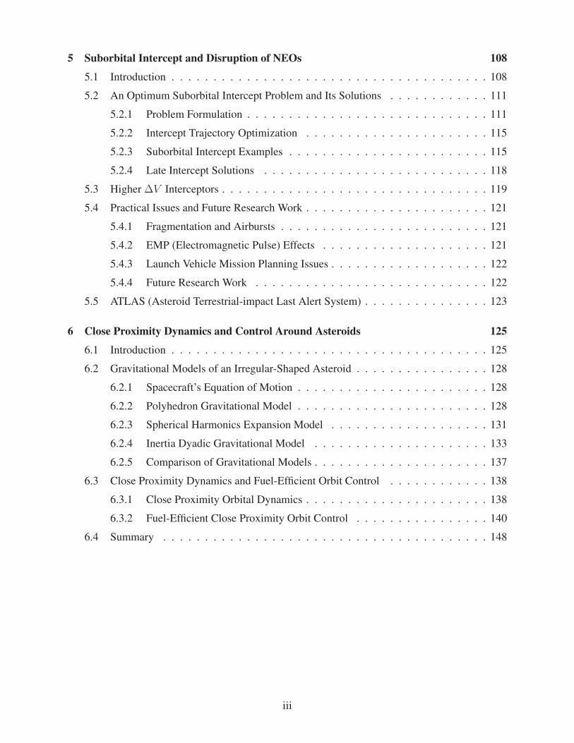
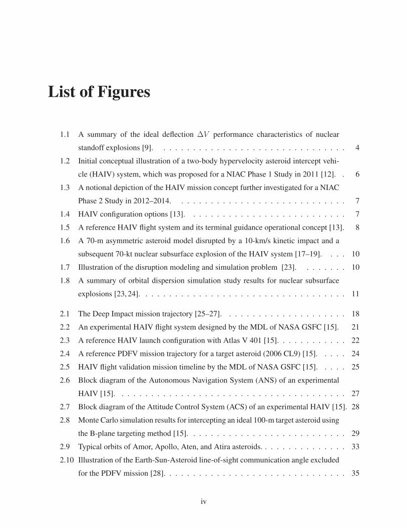
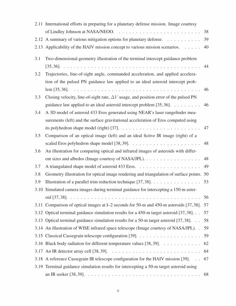
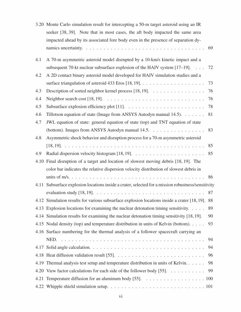