Engineering Costs and Production Economics, 11 (1987) 69-78 Elsevier Science Publishers B.V., Amsterdam - Printed in The Netherlands

69

AN INPUT-OUTPUT MODEL FOR EQUIPMENT REPLACEMENT DECISIONS

J.M.A. Tanchoco

School of Industrial Engineering, Purdue University, West Lafayette, IN 47907 (U.S.A.)

and

L.C. Leung

Department of General Business Management, The Chinese University of Hong Kong, Shatin, New Territories (Hong Kong)

ABSTRACT

This paper provides an approach to equip- equipment replacement decisions. Specifically, ment replacement decisions based on input- a replacement model is developed which in- output analysis. Replacement decision is cast corporates factors such as input substitution, within the framework of production technol- expansion of output, product price-volume ogy selection by examining the input-output relationship, and obsolescence and deteriora- requirements for the production system. The tion effects. The optimal replacement policy proposed approach explicitly integrates pro- is to maximize the terminal wealth of a ma- duction and investment possibilities in to chine tool over a specified planning horizon.

1. BACKGROUND

Traditional equipment replacement analysis originated from the early papers of Taylor [ 1 ] and Hotelling [ 21. Their work established the criterion of maximizing the present value of the machine’s earnings minus its operating and capitalized cost. Their analyses dealt with a single machine life cycle, i.e., the economic life. Preinreich [3 I later showed that the determination of the economic life of a single machine is dependent on the economic life of each machine in the chain of future replace- ments.

The important contribution of extending the model to account for equipment obsoles-

0167-188X/87/$03.50 0 1987 Elsevier Science Publishers B.V.

cence was provided by Terborgh [4] . Ter- borgh contended that the replacement of an existing machine, the defender, should be conditioned by a comparison of its perform- ance with that of the latest new available machine, the challenger. That is, the growth in the inferiority of an old asset relative to the initial performance of the latest equipment is a key factor in the analysis. Terborgh’s in- feriority growth factor consists of two com- ponents: obsolescence and deterioration.

In the post-Terborgh literature, many proposed models [ 5-81 did not depart from the study of the replacement of identical ma- chine types, i.e., like-for-like equipment. Smith [6] later indicated that since a physical

70

equipment is a fixed input to a production process, the choice of equipment could affect the production technology itself and vice- versa. Smith formulated the like-for-like re- placement problem within the framework of production theory and derived several eco- nomic interpretations. The discussion in this paper will follow this framework as it applied to the replacement of identical as well as non- identical machines. The input-output require- ments for a machine form the basis for the replacement model presented. Specifically, the profitability of a production system over a planning horizon is to be determined sub- ject to the input-output transformation process, i.e. the production function, over a planning period.

The role of production function is vital in this replacement approach. It integrates the effects of inputs and outputs into the replace- ment decision. They jointly determine whether or not new equipment should be acquired. Viewed from this perspective, the selection of the replacement chain is parallel to the selec- tion of a sequence of production functions over the planning period. This approach to replacement analysis represents a major departure from the traditional approach. Explicitly examined are several important issues such as: (a) input-oriented issues: capital-labor intensity, effects of input-price changes, and cost allocation; and (b) output- oriented issues: capacity expansion, changes in product demand, and economies of scale.

In the sections to follow, discussion on the optimality criterion, output policy, possibility of input substitutions, and the use of produc- tion functions are provided. ‘A Loentief-type production function [9] is applied where obsolescence and deterioration rates are re- flected through the input-output coefficients. The model determines an optimal replace- ment policy which will minimize the terminal wealth of a production process over a speci- fied finite planning horizon.

2. FACTORS IN EVALUATING REPLACE- MENT POLICIES

The choice of criterion is critical to the evaluation of a replacement policy. Two major economic criteria are frequently em- ployed - cost minimization and profit maxi- mization. Cost minimization involves the minimization of the aggregate discounted value of the initial investment, salvage value and operating costs of a machine or machines. The profit maximization objective includes the revenue component with the goal of maxi- mizing the discounted value of total profit, i.e. total revenue minus both capitalized and operating costs

The two criteria are unique but are equiv- alent under certain conditions. In general, if the revenue is constant, then cost minimiza- tion is in effect the same as profit maximiza- tion The implication is that price is independ- ent of output quantity. In short, the validity of applying either criterion depends largely upon the price-volume relationship of the product and the economic market place.

Whether or not the output level and the revenue generated are altered in any way by the replacement decision is critical to the eco- nomic evaluation of a replacement policy. If neither output level nor selling price is changed by the replacement, then the replacement decision can only be influenced by the rele- vant cost considerations since total revenue would remain constant. In fact, before assess- ing the appropriate criterion for any replace- ment evaluation, the required output level needs to be defined. Based on output level, re- placement decisions may be categorized as (a) replacement without expansion, and (b) ex- pansion with and without replacement.

2.1. Replacement without expansion

When a replacement activity does not cor- respond to a change in output level, it is view-

71

ed as replacement without expansion. This replacement situation implies that there is no desire to increase the output level by virtue of the replacement. It should be noted that the new machine may provide a lower, equal, or higher capacity and may also provide a more efficient means of production.

2.2, Expansion with and without replacement

If an increase in the output level is brought about by virtue of replacement, then this is termed as expansion with replacement, or more appropriately, replacement with expan- sion. Replacement is required since the desired output level exceeds the capacity of the exist- ing machine. In fact, a primary motivation for replacing an existing machine may be to real- ize an increase in total profit by decreasing the unit selling price, which could in turn in- crease the demand for the product. In such a situation, the capacity of the new machine must be greater than or equal to the desired output level. Expansion may also be brought about by retrofitting an existing machine. This case will not be considered in this paper.

When the output capacity is increased due to greater utilization of an existing equip- ment, this is considered an expansion without replacement. This category is included since it is a practical alternative to replacing an exist- ing equipment. Alteration of output capacity can also affect the input requirements.

Examining replacement problems utilizing production functions enables one to investigate the effects on input requirements, or more specifically the input substitutions that may occur, in order to attain a desired output level. This is an area that has received very little attention in the engineering economy literature.

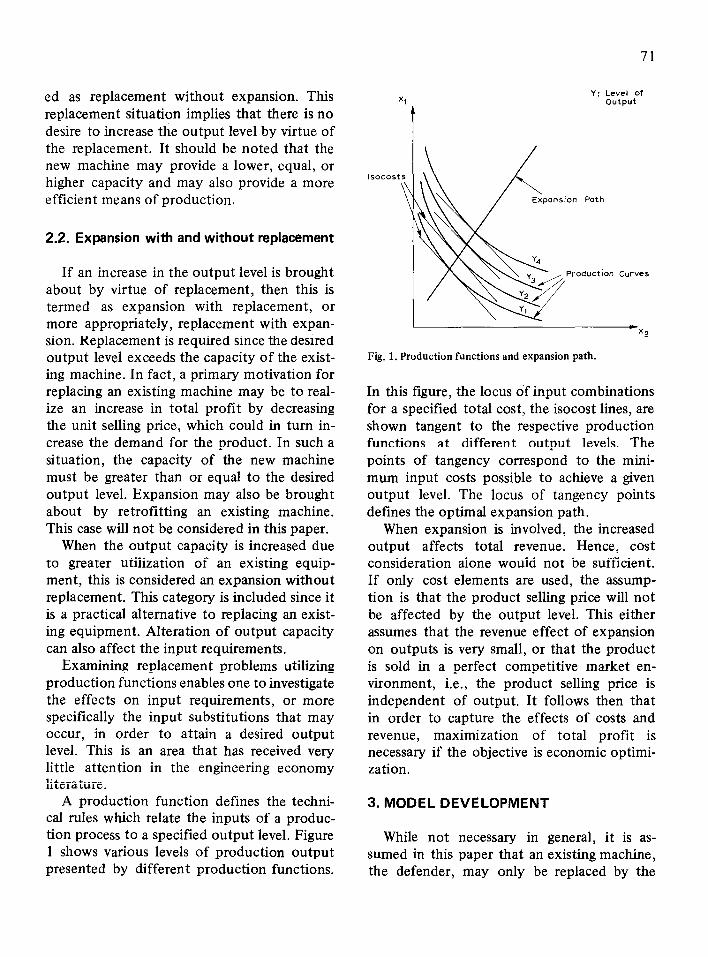
A production function defines the techni- cal rules which relate the inputs of a produc- tion process to a specified output level. Figure 1 shows various levels of production output presented by different production functions.

Y: Level of output

Production Curves

Fig. 1. Production functions and expansion path.

In this figure, the locus of input combinations for a specified total cost, the isocost lines, are shown tangent to the respective production functions at different output levels. The points of tangency correspond to the mini- mum input costs possible to achieve a given output level. The locus of tangency points defines the optimal expansion path.

When expansion is involved, the increased output affects total revenue. Hence, cost consideration alone would not be sufficient. If only cost elements are used, the assump- tion is that the product selling price will not be affected by the output level. This either assumes that the revenue effect of expansion on outputs is very small, or that the product is sold in a perfect competitive market en- vironment, i.e., the product selling price is independent of output. It follows then that in order to capture the effects of costs and revenue, maximization of total profit is necessary if the objective is economic optimi- zation.

3. MODEL DEVELOPMENT

While not necessary in general, it is as- sumed in this paper that an existing machine, the defender, may only be replaced by the

72

latest machine(s), challengers, available. This assumption is made to underline the effect of technological obsolescence on the replace- ment policy. Also, it is assumed that both the defender and challengers are single machines. The option of leasing is not considered, and the physical lives of all machines are assumed to exceed the planning horizon.

In the modeling of cash flows, the end-of- period convention is assumed for all operating revenues and costs with the exception of the initial equipment purchase cost which is a beginning-of-period disbursement. The time periods are discrete and the decision to keep or replace the defender is made at the begin- ning of the period.

The symbols used throughout this paper are based on the triple (i,j,t), were i denotes the machine types, j denotes the age index and t denotes the period of operation. The triple (i,j,t) denotes the ith machine type, made in time period j, and operated in time period t. It is assumed that there are y1 ma- chines types. Thus, i = 1, 2, . . . . n; j = 1, 2, . . . . t; and t = 1, 2, . . . . T where T is a specified planning horizon. Additionally, the symbol * is used to identify the defender machine. Thus, the triple (i*,j*,t) denotes the defender machine operated in period t.

In the following sections, a discussion is made on the revenue and cost components of a production process requiring labor and capital equipment as inputs. The end-of- period future worths for the defender and challengers are subsequently derived. Next, the combinatorial nature of the replacement decision is discussed. Then the criterion for determining an optimal replacement policy is defined and the objective function formulated. The production constraints are then specified. An example illustrating the model developed is included.

3.1. Replacement alternatives and the

production process

The operating profit in period t based on Y units of a single product requiring labor and equipment (capital) inputs is given by

OW,t) = p(i,j,t)YW,t) - ~w,(r)x,(i,Lt) + dWmW,t) 1 (1)

where Y(ij,t) = the output level (production = sales), p(i,j, t) = the product selling price, WI(t) = the price of labor in period t, x,(ij,t) = the amount of labor input in period t, d(t) =

the price of equipment maintenance in period t, and m(i,j,t) = the amount of maintenance input in period t.

Defining n(t) as the wealth (future worth) at the end of period t (except the last period corresponding to the end of planning horizon 13,

@(i*,i*,t) + (1 + ~)n (t - l), for the defender; n(t) = and @(i,t,r) - (1 + ~)[W(i,f,t) - W*J*,r - 111 + (*I

(1 + p)n(t - l), for the ith replacement altema- tive, VI = 1,2,...)1

where p = the reinvestment rate, W(i,t,t) = the

initial outlay for the ith challenger, and S(i*j*,t - 1) = the salvage value of the de- fender machine at the beginning of period t.

3.2. Terminal wealth maximization

Specifying T as the planning horizon, there are T decision periods. At the beginning of each of these periods, the firm must decide to either keep the defender or replace the de- fender with one of y1 available challengers in such a way that the terminal wealth, n(T), is maximized, that is,

Maximize IT( 7) where

keep: @(i*,j*,r) + S(i*,j*,T) + (1 + p)n(t- l), and n(T) = replace: @(i,T,T) + S(i*j*,T- 1) - W(i,T,?J (3)

+ S(i,T,T) + (1 + p)n(t - l), VI = 1,2 ,..., n

73

3.3. Economic factors and allocation constraints

In this section, the functional relationship are developed for (a) input and output rela- tionships, (b) labor and maintenance coeffi- cients, (c) price of labor and maintenance in- puts, (d) machine capacities, (e) price-volume relationships, (t-9 machine values, and (g) labor and maintenance availability.

3.3.1. Input-output relationships

Define a(ij,t) as the labor coefficient and b(ij,t) as the maintenance coefficient. The labor and maintenance required are assumed to vary linearly with the output level. This is commonly known as a Leontief-type produc- tion function. For the defender,

x,(i*j*,t) = ~l(i”,j*,t)Y(i*j*,t), and m(i*,j*,t) = b(i*j*,t)Y(i*,j*,t);

and for the ith challanger,

x,(i,t,t) =u(i,t,t)Y(i,t,t), and m(i,t,t) = b(i,t,r)Y(i,t,t). VI = 1,2,...,n

for the defender with respect to the chal- lengers.

3.3.3 Price of labor and maintenance input

It is assumed that the prices of both labor, wl(t), and maintenance, d(t), are known and that their values are constant within each period but are subject to variations between. periods.

3.3.4 Machine capacity

All machine capacities, Q(ij.t> are assumed to be known. Additionally, the machine capacity of the defender machine is assumed to remain the same as it was originally pur- chased, i.e.,

Q(i*,j*,t) = Q(i*,j*,t - 1) = . . . . = Q(i*,j*,j*,.

The capacities of each challenger available at each end-of-period t are also assumed identi- cal, i.e.,

Q(l,t,t) = Q(Z,t,r) = . . . = Q(n,t,t)

The conditions above imply that capacity changes can only occur through replacements.

3.3.2 Labor and maintenance coefficients 3.3.5 Price-volume relationships

In general, for the defender, these values would increase monotonically from period to period, i.e.,

a(i*j*,j*) < a(i*,j*,j* + 1) C . . . . < a(i*,j*,t), and b(i*j*j*) < b(l*j*j* + 1) < . . . . < b(i*,j*,t).

The increasing values of both labor and maintenance coefficients indicate the effects of deterioration. On the other hand, for the challengers, these values would decrease monotonically from period to period, i.e.,

a&1,1) > a&2,2) > . . . > n&t&, and b&111) > b&2,2) 2 . . . > b(i,t,t).

The decreasing values indicate technological change. The combination of these two effects is commonly known as the inferiority growth

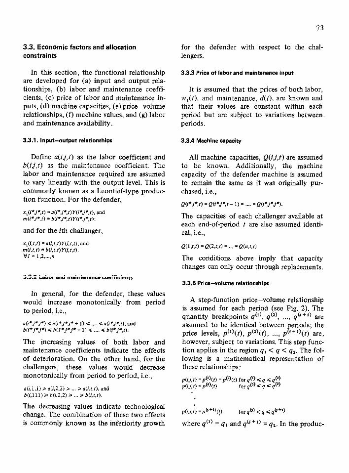
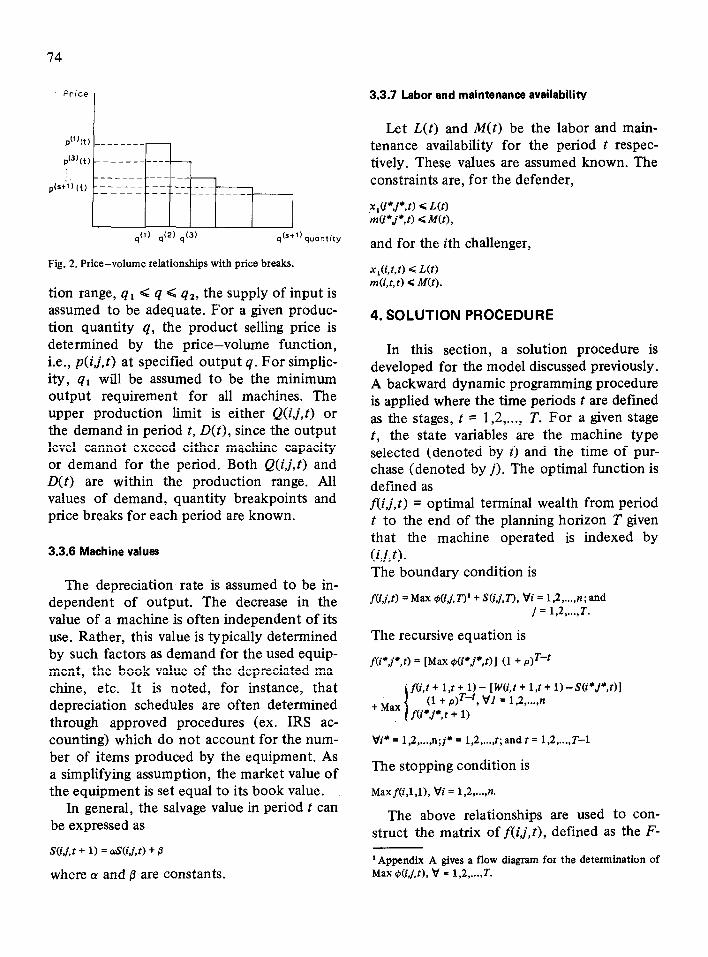
A step-function price-volume relationship is assumed for each period (see Fig. 2). The quantity breakpoints q(l), qt2), . . . . q(‘+‘) are assumed to be identical between periods; the price levels, p(‘)(t) pc2)(t) p@ ‘l)(t) are, however, subject to’variatidn~.‘This step func- tion applies in the region q1 < (I < q2. The fol- lowing is a mathematical representation of these relationships:

p(ij,t) = p@(r) = p@(t) for q(l) < * 4 q(a) p(ij,r) = p(%) for @) < 4 < (I(‘)

p&j,;) =pQ+%{) for cp) <q < @+I)

where q(l) = q1 and q(’ + ‘) = q2. In the produc-

74

Price 3.3.7 Labor and maintenance availability

Fig. 2. Price-volume relationships with price breaks.

tion range, q1 Q 4 < q2, the supply of input is assumed to be adequate. For a given produc- tion quantity 4, the product selling price is determined by the price-volume function, i.e., p(ij,t) at specified output 4. For simplic- ity, q1 will be assumed to be the minimum output requirement for all machines. The upper production limit is either Q<i,j,t> or the demand in period t, D(t), since the output level cannot exceed either machine capacity or demand for the period. Both Q(i,j,t> and D(t) are within the production range. All values of demand, quantity breakpoints and price breaks for each period are known.

3.3.6 Machine values

The depreciation rate is assumed to be in- dependent of output. The decrease in the value of a machine is often independent of its use. Rather, this value is typically determined by such factors as demand for the used equip- ment, the book value of the depreciated ma- chine, etc. It is noted, for instance, that depreciation schedules are often determined through approved procedures (ex. IRS ac- counting) which do not account for the num- ber of items produced by the equipment. As a simplifying assumption, the market value of the equipment is set equal to its book value.

In general, the salvage value in period t can be expressed as

s(i,j,r + 1) = orS(ij,f) + p

where (Y and p are constants.

Let L(t) and M(t) be the labor and main- tenance availability for the period t respec- tively. These values are assumed known. The constraints are, for the defender,

x,CP,j*,t1 <L(f) m(i*j*,t) 6 M(t),

and for the ith challenger,

4. SOLUTION PROCEDURE

In this section, a solution procedure is developed for the model discussed previously. A backward dynamic programming procedure is applied where the time periods t are defined as the stages, t = 1,2 ,..., T. For a given stage t, the state variables are the machine type selected (denoted by i) and the time of pur- chase (denoted by j). The optimal function is defined as f(i,j,t) = optimal terminal wealth from period t to the end of the planning horizon T given that the machine operated is indexed by (W). The boundary condition is

fcij,U = Max &ij, TY + S(ij,TI, Vi = 1,2 ,..., II ; and j = 1,2 ,..., T.

The recursive equation is

f(i*,j*,r) = [Max @(i*j*,t)] (1 + p)T-t

fO,t+ l,t+ l)- [W&r+ l,t+ l)-S(i*j*,t)]

+ Max (1 + p)T-‘, VI = 1 2 , ,...,n

fv,j*,t + 1) 1

Vi* = 1,2 ,... ,n;j* = 1,2 ,..., t; and t = 1,2 ,..., T-l

The stopping condition is

Maxf(i,l,l), vi = 1,2 ,..., n.

The above relationships are used to con- struct the matrix of f(i,j,t), defined as the F-

‘Appendix A gives a flow diagram for the determination of Max @(ij,f), V = 1,2 ,..., T.

matrix. The optimal terminal wealth would be reflected by the maximum of Ai,l,l) Vi = 1,2,...,n. The optimal replacement policy can then be obtained by retracing the paths that lead to the optimal decision. Additionally, the optimal output levels of the correspond- ing machines in the chain of replacements would indicate the expansion/contraction policy of the firm. This is determined when the optimal operating profits for each ma- chine in each period are computed.

5. AN ILLUSTRATIVE EXAMPLE

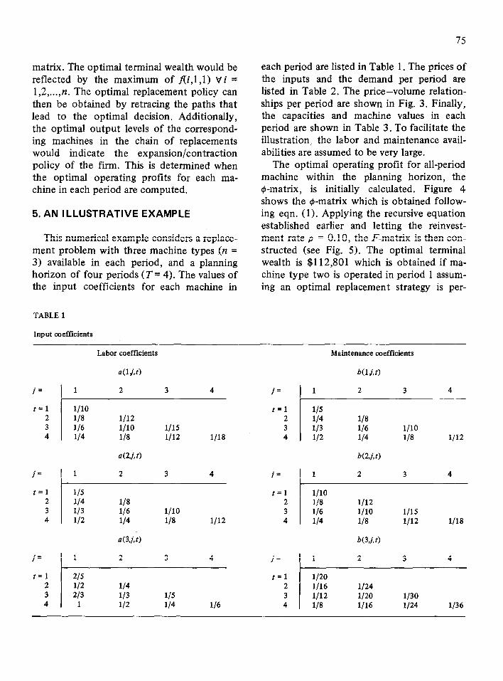
This numerical example considers a replace- ment problem with three machine types (n = 3) available in each period, and a planning horizon of four periods (T = 4). The values of the input coefficients for each machine in

TABLE 1

Input coefficients

75

each period are listed in Table 1. The prices of the inputs and the demand per period are listed in Table 2. The price-volume relation- ships per period are shown in Fig. 3. Finally, the capacities and machine values in each period are shown in Table 3. To facilitate the illustration, the labor and maintenance avail- abilities are assumed to be very large.

The optimal operating profit for all-period machine within the planning horizon, the #-matrix, is initially calculated. Figure 4 shows the $-matrix which is obtained follow- ing eqn. (1). Applying the recursive equation established earlier and letting the reinvest- ment rate p = 0.10, the F-matrix is then con- structed (see Fig. 5). The optimal terminal wealth is $112,801 which is obtained if ma- chine type two is operated in period 1 assum- ing an optimal replacement strategy is per-

j=

t=1 2 3 4

o(U t) KUt)

2 3 4 j=

r=1 118 2 l/6 l/10 3 l/4 l/8 l/12 4

fl

a(3,jA b(3,W

Labor coefficients Maintenance coefficients

a(lj,r) b(lj,t)

;I; j ::; ;[ ; ;$ :I)

76

formed from there on. The task then is to trace this replacement chain starting from machine type two in year one. According to

Price

7 Quantity 1000 3000 5000 7000 9000 11000

1000 3000 5000 7000 9000 11000

Fig. 3. Price-output relationships by period.

A- j = periods of make

i, t = periods of use machine

type

f(2,l ,l), this value is obtained only when the decision in the next period, year two, is to replace the defender by machine type 1. Sim-

TABLE 2

Labor input rate, maintenance rate and demand for each yeas

w&) d(t) D(t)

t=1 5 I 7000 2 I 8 8000 3 10 9 9000 4 14 10 10000

TABLE 3

Machine capacities and machine values

j=l 2 3 4

t=l 9000 Machine capacities 2 9000 10000 for all types 3 9000 10000 11000

4 9600 10000 11000 12000

r=l Machine values 2 for all types 3

4

j=l 2 3 4

25000 20000 40000 15000 30000 60000 10000 20000 40000 80000

5000 10000 20000 40000

A-- j. period of make

n t_ / it

machine = period of use

“SC

i,,,4,1

---* l?epbxc

- Keep

Fig. 4. Matrix of optimal operating profit. Fig. 5. F-matrix for 10% reinvestment rate.

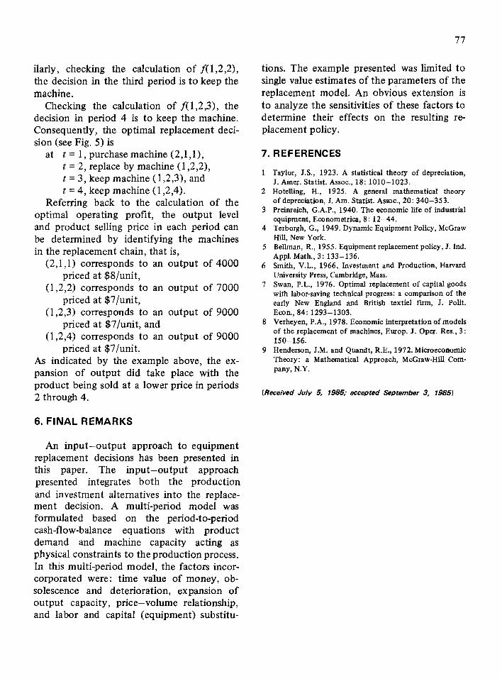
ilarly, checking the calculation of f(l,2,2), the decision in the third period is to keep the machine.

Checking the calculation of f( 1,2,3), the decision in period 4 is to keep the machine. Consequently, the optimal replacement deci- sion (see Fig. 5) is

at t = 1, purchase machine (2,l ,l>, t = 2, replace by machine (1,2,2), t = 3, keep machine ( 1,2,3), and t = 4, keep machine (1,2,4).

Referring back to the calculation of the optimal operating profit, the output level and product selling price in each period can be determined by identifying the machines in the replacement chain, that is,

(2,1,1) corresponds to an output of 4000 priced at $8/unit,

(1,2,2) corresponds to an output of 7000 priced at $7/unit,

(1,2,3) corresponds to an output of 9000 priced at $7/unit, and

(1,2,4) corresponds to an output of 9000 priced at $7/unit.

As indicated by the example above, the ex- pansion of output did take place with the product being sold at a lower price in periods 2 through 4.

6. FINAL REMARKS

An input-output approach to equipment replacement decisions has been presented in this paper. The input-output approach presented integrates both the production and investment alternatives into the replace- ment decision. A multi-period model was formulated based on the period-to-period cash-flow-balance equations with product demand and machine capacity acting as physical constraints to the production process. In this multi-period model, the factors incor- corporated were: time value of money, ob- solescence and deterioration, expansion of output capacity, price-volume relationship, and labor and capital (equipment) substitu-

77

tions. The example presented was limited to single value estimates of the parameters of the replacement model. An obvious extension is to analyze the sensitivities of these factors to determine their effects on the resulting re- placement policy.

7. REFERENCES

Taylor, J.S., 1923. A statistical theory of depreciation, J. Amer. Statist. Assoc., 18: 1010-1023. HoteIling, H., 1925. A general mathematical theory of depreciation, J. Am. Statist. Assoc., 20: 340-353. Preinreich, G.A.P., 1940. The economic life of industrial equipment, Econometrica, 8: 12-44. Terborgh, G., 1949. Dynamic Equipment Policy, McGraw HiII, New York. Bellman, R., 1955. Equipment replacement policy, J. Ind. Appl. Math., 3: 133-136. Smith, V.L., 1966, Investment and Production, Harvard University Press, Cambridge, Mass. Swan, P.L., 1976. Optimal replacement of capital goods with labor-saving technical progress: a comparison of the early New England and British textiel firm, J. Polit. Econ., 84: 1293-1303. Verheyen, P.A., 1978. Economic interpretation of models of the repkcement of machines, Europ. J. Oper. Res., 3: 150-156. Henderson, J.M. and Quandt, R.E., 1972. Microeconomic Theory: a Mathematical Approach, McGraw-Hill Com- pany, N.Y.

(Received July 5, 1985; accepted September 3, 1985)

78

APPENDIX A Flow Diagram for the Determination of Max $(i,j,t), t= 1.2, . . . , T

Kirl 1 I

REVENUES COSTS