Favoritenstraße 9-11 / E186, A-1040 Wien, AustriaTel. +43 (1) 58801-18601, Fax +43 (1) 58801-18699www.cg.tuwien.ac.at

Forschungsbericht / Technical Report

TECHNISCHE UNIVERSITÄT WIENInstitut für Computergraphik und Algorithmen

An Integer Linear ProgrammingApproach and a Hybrid VariableNeighborhood Search for the Car

Sequencing Problem

Matthias Prandtstetter and Gunther R. Raidl

TR–186–1–05–01

23. November 2005

An Integer Linear Programming Approach

and a Hybrid Variable Neighborhood Search

for the Car Sequencing Problem ⋆

Matthias Prandtstetter, Gunther R. Raidl

Vienna University of Technology,Institute of Computer Graphics and Algorithms,

Favoritenstrasse 9–11 / E186–1, A–1040 Vienna, Austriahttp://www.ads.tuwien.ac.at

Abstract

In this paper we present two major approaches to solve the car sequencing problem,in which the goal is to find an optimal arrangement of commissioned vehicles alonga production line with respect to constraints of the form “no more than lc cars areallowed to require a component c in any subsequence of mc consecutive cars”. Thefirst method is an exact one based on integer linear programming (ILP). The secondapproach is hybrid: it uses ILP techniques within a general variable neighborhoodsearch (VNS) framework for examining large neighborhoods. We tested the twomethods on benchmark instances provided by CSPlib and the automobile man-ufacturer RENAULT for the ROADEF Challenge 2005. These tests reveal thatour approaches are competitive to previous reported algorithms. For the CSPlib

instances we were able to shorten the required computation time for reaching andproving optimality. Furthermore, we were able to obtain tight bounds on some ofthe ROADEF instances. For two of these instances the proposed ILP-method couldprovide new optimality proofs for already known solutions. For the VNS, the indi-vidual contributions of the used neighborhoods are also experimentally analyzed.Results highlight the significant impact of each structure. In particular the largeones examined using ILP techniques enhance the overall performance significantly,so that the hybrid approach clearly outperforms variants including only commonlydefined neighborhoods.

Key words: Car Sequencing Problem, Integer Linear Programming, VariableNeighborhood Search, Hybrid Meta-heuristics

⋆ This work is supported by the RTN ADONET under grant 504438.Email addresses: prandtstetter@ads.tuwien.ac.at (Matthias Prandtstetter),

raidl@ads.tuwien.ac.at (Gunther R. Raidl).

Preprint submitted to Elsevier Science 26 February 2007

1 Introduction

In automobile industry a cost-effective arrangement of commissioned carsalong the production line is desired. Although the individual cars are similar,each automobile requires particular components to be installed by differentworking bays along the assembly line. In addition to the different configura-tions of cars to be arranged along the production line, each vehicle has to bepainted with exactly one color. The arising problem in which the goal is tominimize the number of color changes while considering the constraints de-fined by various working bays is called car sequencing problem (CarSP). Afeasible solution to CarSP is a permutation of all cars to be produced at acertain day taking all constraints into consideration.

The production line itself consists of three stages: the body shop, the paintshop, and the assembly shop. In the body shop the chassis of the cars aremanufactured, the paint shop workers paint the cars, and in the assembly shopdifferent options like air condition, sun roofs, or sound systems get installed.The constraints defined by the body shop and the assembly shop are similarto each other, whereas the paint shop constraints differ significantly. For theformer, we consider restrictions which can be expressed as “No more than lccars are allowed to require component c in any sequence of mc consecutive

cars.” For the latter, we consider constraints of the form: “At most s cars with

the same color are allowed to be arranged consecutively.” Changing the colorafter at most s cars is motivated by a more psychological reason: In automobileindustry, the paint of a car is applied using an injector. During this sprayingthe paint slowly agglutinates. To obtain good results the injector has to becleaned in regular intervals. If the same color would be applied after cleaningthe injector again, the staff concerned with the cleaning process would getimprecise, because “It’s the same color again.” This leads to improper paintingresults, which consequently evoke reclamations.

In Section 2 we first give a formal definition of CarSP, and in Section 3 wepresent a brief literature review. Section 4 proposes a new integer linear pro-gramming (ILP) formulation whose solution with the general purpose ILPsolver CPLEX yields proven optimal solutions for small and medium-sizedproblem instances. For dealing with larger instances, a second approach basedon general variable neighborhood search (VNS) is introduced in Section 5.Several types of neighborhoods are presented: in addition to some adoptedfrom previous work, also new large neighborhoods that are examined by ILPmethods are introduced. For comparison with results found in the literature,we use two different sets of benchmark instances. The first set is taken fromthe publicly available benchmark collection called CSPlib [2]. The other setis taken from the instances proposed by the French Operations Research So-ciety ROADEF and the car manufacturer RENAULT for the ROADEF

2

Challenge 2005 [9]. Experimental results, which are presented in Section 6,indicate that the new ILP approach performs well in comparison to otherexact methods; in particular we were able to approximately halve the timeneeded to solve some of the benchmark instances. The variants of our VNSapproach that include the large neighborhoods examined using ILP techniquesare shown to outperform those considering only traditional structures. In fact,an experimental analysis indicates that each neighborhood we propose in thisarticle usually contributes significantly to the overall success. In particular, theVNS-variant including all neighborhoods turns out to be competitive to theleading algorithms from the ROADEF Challenge 2005. Conclusions completethis article.

2 Formal Definition

In this section, we present a formal definition of CarSP. The notation intro-duced here will be used throughout the whole document.

Given are a set of possible components C, including a set of colors F ⊆ C,and a set K of requested configurations

K = {k : k ⊆ C, |k ∩ F | = 1} ,

i.e. each configuration k is a subset of components to be installed, and exactlyone color is selected in each configuration.

If configuration k contains component c, a corresponding 0–1 constant ack

is set to 1, otherwise to 0. Component vector aTk = (a0k, . . . , a|C|k) denotes

the incidence vector for configuration k. Let function H(aTi , aT

j ) be the Ham-ming distance of two configurations i and j. All configurations requested inan instance of CarSP are pairwise different, i.e. H(aT

i , aTj ) ≥ 1, for all pairs

(i, j) ∈ K2, i 6= j, and for each k ∈ K there is further given an integer demandδk ≥ 1 indicating how many vehicles of configuration k have to be produced.

A solution to CarSP is a mapping X = (x1, . . . , xn) : {1, . . . , n} → K specify-ing a sequence of length n =

∑

k∈K δk, which assigns exactly one configurationk ∈ K to each position i = 1, . . . , n. Since only commissioned cars shall beproduced, the restriction |{xi : xi = k}| = δk, for all k ∈ K, has to be ful-filled. Furthermore, the number of consecutive cars painted with the samecolor f ∈ F has to be less than or equal to the maximum color block size s.

For each component c ∈ C we are given a sliding window length mc ∈ N

and a quota lc ∈ N. Only lc cars are allowed to require component c in anysubsequence of mc consecutive vehicles. Due to the constraints defined by the

3

paint shop lf is equal to s and mf is equal to s + 1 for all colors f ∈ F . Wedenote the total demand of any component c ∈ C by dc =

∑

k∈K ack · δk.

The production of the last day needs to be considered. For this purpose addi-tional constants eci ∈ {0, 1}, c ∈ C, i = 1, . . . ,mc − 1, are used: eci is set to 1iff the i-th last car of the previous day required component c.

Often CarSP is formulated as an optimization problem in which the totalcosts of color changes and weighted assembly shop constraint violations haveto be minimized. For this purpose, we associate constant costs γf > 0, f ∈ F ,with a change to color f and costs γc > 0, c ∈ C \ F , with a violation of anassembly shop constraint. The goal is to find a sequence X of commissionedcars minimizing the objective function

obj(X) =n

∑

i=1

costs(i) (1)

with the costs for each position i being

costs(i) = change(i) +∑

c∈C\F

viol(i, c), (2)

change(i) =

γf · maxf∈F

{

afx1− ef11

}

if i = 1

γf · maxf∈F

{

afxi− afxi−1

}

otherwise(3)

viol(i, c) =

γc · max

{

0,i

∑

j=i−mc+1acxi

− lc

}

if i ≥ mc

γc · max

{

0,i

∑

j=1acxi

+mc−i∑

j=1ecj − lc

}

otherwise(4)

under the remaining hard constraints

i∑

j=1

afxj+

s−i+1∑

j=1

efj ≤ s for i = 1, . . . , s (5)

i∑

j=i−s

afxj≤ s for i = s + 1, . . . , n (6)

ensuring that no more than s cars of the same color are scheduled in a row.Expression change(i) represents the costs for a potential color change at posi-tion i of sequence X and viol(i, c) denotes the costs for possible assembly shopconstraint violations at position i with respect to component c. The latter arecomputed as the sum of cars requiring component c within the last mc cars(including the car at position i) minus the quota lc; if this difference is lessthan 0, the number of violations is set to 0.

Note that for computing the costs of color changes considering not only thenew color to but also the color of the previous car would be more precise. Since

4

typically color changes are penalized using a constant factor independently ofthe involved colors, we use this simplified problem description.

3 Previous Work

Gent [1] showed that the decision problem associated with the car sequencingproblem whether there exists an optimal solution without any violations ofthe constraints defined by the assembly line is NP-hard. Kis [8] proved thatthis decision problem is NP-hard in a strong sense, and Hu [6] stated that theoptimization problem including the color constraints as defined in Section 2is NP-hard, too.

Several different approaches have been made to solve CarSP or variants ofit. The methods used vary from greedy heuristics to meta-heuristics like antcolony optimization, whereas only a few exact algorithms have been described.

3.1 Exact methods

Gravel et al. [4] proposed an ILP approach for a variant of CarSP without theconstraints specifically related to the paint shop. It is able to solve commonlyused benchmark instances with about 200 cars and 5 components to provenoptimality within practically reasonable time. The main idea applied in thisformulation is to group cars with the same configuration into classes to avoidsymmetries.

Hu [6] describes another ILP approach that also takes constraints defined bythe paint shop into account. Unfortunately, the size of practically solvableinstances is limited to about 30 cars with 8 components.

Another exact ILP approach is presented in [12], which, in contrast to theapproach by Hu and analogously to the formulation of Gravel et al., classifiescars with the same configuration into groups. Thereby, the size of practicallysolvable instances is enlarged to at most 300 cars with about 8 components.

3.2 Greedy heuristics

Gottlieb et al. [3] proposed greedy heuristics using different evaluation strate-gies. They construct sequences of cars by always adding the next best carin respect to some evaluation function to a current partially filled sequence.Once a car is placed at a position, it is never reconsidered again. Some of

5

the proposed evaluation functions take the currently available cars and thealready existing partial sequence into account, whereas others only computea global value indicating whether a car is hard to arrange without constraintviolations or not.

Many other approaches like the following local search based techniques utilizesimilar greedy heuristics for computing initial solutions.

3.3 Local search based methods

Many attempts for solving CarSP are based on the concept of local search.Puchta et al. [3,13] proposed an approach that makes use of six different typesof neighborhood structures which are defined by the following moves: exchang-ing two cars (swap moves), removing one car and inserting it at another posi-tion (insert move), swapping to consecutive cars (transposition moves), swap-ping two cars similar with respect to their configuration (similar swap moves),inverting a subsequence of cars (Lin2Opt moves) and randomly rearrangingcars in a subsequence (random move). Within a local search framework, thetype of move and the affected positions are chosen at random. In contrast,Jaskiewicz et al. [7] decide the initial position, where the move is applied to,by means of a greedy heuristic. Then they look for the best move to be appliedat this position.

Perron et al. [10] define similar moves, but they apply them to subsequences,i.e. swap moves exchange two subsequences of cars and insert moves shift asubsequence of cars to another position.

In [12], we presented a general variable neighborhood search approach forCarSP, which combines well known neighborhood structures with newly de-fined ones examined using ILP techniques. The current article extends thiswork and discusses several aspects in more detail. For instance, the conclu-sions drawn by investigating preliminary results presented in [12] were usedto adjust and refine the applied search parameters and data structures forevaluating single (improvement) moves. New variants of utilized neighbor-hood structures where included within the VNS approach as proposed in thisarticle. Furthermore, a new ILP formulation is presented.

3.4 Ant colony optimization

Gravel et al. [4] and Gottlieb et al. [3] presented different variants of antcolony optimization (ACO) approaches for CarSP. The proposed variants dif-fer in the local heuristics they apply for selecting the next car and in the

6

neighborhoods used during local search. The iterative solution constructionprocess is guided by local heuristics, pheromone information, and random de-cisions. A pheromone value is maintained for each ordered pair of cars, and itis strengthened when in good candidate solutions the second car is scheduleddirectly after the first. In some variants of this ACO approach, each candidatesolution as well as the final result is further improved by local search.

4 A New Integer Linear Programming Formulation

This section introduces a new ILP formulation for CarSP. We will later see thatfor many practical instances it can be significantly faster solved to optimalitythan previous formulations. This new ILP formulation differs from the previousones therein that the assignment of individual components to positions ofthe production line is emphasized. Suitable constraints guarantee that thecommissioned cars are produced.

The following variables are used: For each position i ∈ {1, . . . , n} and eachcomponent c ∈ C, 0–1 variables bci indicate whether component c is to beinstalled at the i-th car (bci = 1) or not (bci = 0). Furthermore, for eachk ∈ K and each position i ∈ {1, . . . , n} a binary variable pki is set to 1 iffthe components assigned to position i correspond to configuration k. For eachcomponent c ∈ C \ F and position i ∈ {1, . . . , n} variable gci represents thenumber of constraint violations occurring at the corresponding position withrespect to the constraints defined for component c. A binary variable wfi isset to 1 iff a change to color f occurs at position i.

The formulation as an integer linear program is as follows:

min∑

c∈C\F

γc ·n

∑

i=1

gci +∑

f∈F

γf ·n

∑

i=1

wfi (7)

subject to∑

f∈F

bfi = 1 i ∈ {1, . . . , n} (8)

n∑

i=1

bci = dc c ∈ C (9)

pki ≤ ack · bci + (1 − ack) · (1 − bci) k ∈ K, c ∈ C, i ∈ {1, . . . , n} (10)

bci =∑

k∈K

ack · pki i ∈ {1, . . . , n}, c ∈ C (11)

n∑

i=1

pki = δk k ∈ K (12)

7

gci ≥i

∑

j=1

bcj +

mc−i∑

j=1

ecj − lc i ∈ {1, . . . , mc − 1}, c ∈ C\F (13)

gci ≥i

∑

j=i−mc+1

bcj − lc i ∈ {mc, . . . , n}, c ∈ C\F (14)

wf1 ≥ bf1 − ef1 f ∈ F (15)

wfi ≥ bfi − bf(i−1) i ∈ {2, . . . , n}, f ∈ F (16)i

∑

j=1

bfj +s+1−i∑

j=1

efj ≤ s i ∈ {1, . . . , s}, f ∈ F (17)

i∑

j=i−s

bfj ≤ s i ∈ {s + 1, . . . , n}, f ∈ F (18)

gci ≥ 0 i ∈ {1, . . . , n}, c ∈ C\F (19)

wfi ≥ 0 i ∈ {1, . . . , n}, f ∈ F (20)

bci ∈ {0, 1} c ∈ C, i ∈ {1, . . . , n} (21)

pki ∈ {0, 1} k ∈ K, i ∈ {1, . . . , n} (22)

Objective function (7) corresponds to function obj (X ) in Eq. (1) and aims atminimizing the costs for color changes and constraint violations. Since eachcar has to be painted with exactly one color, constraints (8) are introduced.Equations (9) ensure that in total dc cars requiring component c ∈ C areproduced. Constraints (10) allow variables pki to be set to 1 only if the com-ponents assigned to position i correspond to the requirements of configurationk. In addition, we introduce the equations (11) which guarantee that eachvariable bci is set in accordance to the values of the corresponding variablespki. Equalities (12) assure the production of the correct amount δk of eachconfiguration k ∈ K.

To ensure that the number of occurring constraint violations is correctlycounted we introduce constraints (13), (14) and (19). For counting the correctnumber of color changes, we add inequalities (15), (16) and (20).

Finally, we have to ensure the hard constraints defined by the paint shop,which state that in any subsequence of s + 1 consecutive cars at least onecolor change has to occur. For this purpose, we introduce constraints (17) and(18).

Like for other so far published ILP models the application of this formulationis limited to moderately sized instances with up to 300 cars and about 8components. For approaching larger instances, we also developed an algorithmbased on general variable neighborhood search in which several types of largeneighborhoods are explored via integer linear programming.

8

5 A Heuristic Approach Based on Variable Neighborhood Search

5.1 General Variable Neighborhood Search Framework

General variable neighborhood search (VNS) is a meta-heuristic concept whichfollows the idea of exploiting different neighborhood structures within a localsearch framework in order to escape from local optima. This method was firstproposed by Hansen and Mladenovic, and a detailed introduction can be foundin [5].

Algorithm 5.1: VND(X)

Input: an initial solution XOutput: a local optimum in respect to all available neighborhoods Nt, for

t = 1, . . . , tmax

t ← 1repeat

find X∗ ∈ Nt(X) with f(X∗) ≤ f(X ′), ∀X ′ ∈ Nt(X)if f(X∗) < f(X) then

X ← X∗

t ← 1else

t ← t + 1

until t > tmax

return X

Variable neighborhood descent (VND) is used as a subroutine for finding so-lutions that are local optima with respect to a set of tmax different neighbor-hood structures {N1, . . . ,Ntmax

}. Algorithm 5.1 shows this procedure whichperforms a local search and systematically switches between the neighbor-hoods. Typically, the sizes of the neighborhoods or the time complexities forevaluating them induce a natural order of them such that the smallest orfastest neighborhood is examined first followed by the more complex ones.Different step functions can be applied, but it is most common to choose abest-improvement or a next-improvement strategy.

VND is embedded in the general VNS framework, which uses a second set ofneighborhood structures {N1, . . . , Numax

} and focuses more on diversification,see Alg. 5.2. For escaping local optima, a shaking operation is performed thatrandomly chooses a feasible solution from the u-th neighborhood Nu(X).

Neighborhood structures {N1, . . . , Numax} should be designed in such a way

that the similarity between the incumbent solution X and the candidate solu-tions in Nu(X) decreases with an increasing parameter u. If no improvement

9

Algorithm 5.2: VNS()

Output: the best heuristic solution found

generate initial solution Xrepeat

u ← 1repeat

X ← Shaking(u, X)

X ′ ← VND(X)

if f(X ′) < f(X) thenX ← X ′

u ← 1else

u ← u + 1

until u > umax

until stopping condition is met

return X

i j

Fig. 1. Swap move: Configurations at positions i and j are swapped. All otherconfigurations stay at their positions.

could be achieved during the last VND iteration attempts are made to escapethe current local optimum by steadily increasing u. Otherwise, if the algorithmwas able to find a better solution, it restarts with N1. The whole procedure isrepeated until some stopping criterion is met.

5.2 Neighborhoods for VND

In the following, we present the neighborhood structures N1 to Ntmax, which

are used within VND. They utilize in general three different types of basicmoves: swap, shift, and κ-exchange. In our VNS for CarSP we represent acandidate solution naturally by its configuration vector X = (x1, . . . , xn) andin the following we denote by πi a subsequence of X of arbitrary length, by(xi) the subsequence consisting of a single configuration xi, and by “·” theconcatenation operator.

10

i j

Fig. 2. Backward shift move: One configuration is moved from position j to po-sition i. All configurations between these two positions are shifted one positionbackward.

5.2.1 Swap moves

A swap move SWP(X, i, j) swaps the positions of two configurations in thecurrent arrangement X, see Fig. 1; i.e. configuration xi at position i is ex-changed with configuration xj at position j. The configurations at all otherpositions k, k 6= i and k 6= j, are unaffected by this move:

SWP(

π1 · (xi) · π2 · (xj) · π3, i, j)

= π1 · (xj) · π2 · (xi) · π3 (23)

For saving computation time in the evaluation of neighborhoods induced bythis type of move, we use an incremental method for computing objective val-ues. For this purpose, we define an array of size n · |C|, whose entries representthe number of occurrences of each component c ∈ C within each sliding win-dow of size mc. Thereby, a potential change in the number of violations forcomponent c ∈ C can be computed in constant time. Using a second array ofsize n whose entries point to the first configuration within the current colorblock it is further possible to detect and evaluate potential color changes andviolations of the maximum color block size in constant time. For this purposeit is only necessary to save the length of each color block. In total, evaluatinga single move only takes time O(

∑

c∈C\F mc).

5.2.2 Shift moves

There are two types of shift moves depending on the displacement of the af-fected car: backward shift BSH (X, i, j) and forward shift moves FSH (X, i, j).If a backward shift move is applied to the current arrangement the config-uration at position j is moved to position i with i < j, whereas all cars atlocations k, with k = i, . . . , j − 1, are shifted one position backward along theproduction line, see also Fig. 2:

BSH(

π1 · (xi) · π2 · (xj) · π3, i, j)

= π1 · (xj) · (xi) · π2 · π3 (backward) (24)

The forward shift move is defined correspondingly:

FSH(

π1 · (xi) · π2 · (xj) · π3, i, j)

= π1 · π2 · (xj) · (xi) · π3 (forward) (25)

11

pool

Fig. 3. κ-exchange move: A set of configurations is selected and set free, i.e. put intoa pool. Then these configurations are reassigned to the free positions.

Exploiting the same data structures as for swap moves it is possible to achievean incremental and efficient evaluation of shift moves in time O(

∑

c∈C\F mc).Since it is required to update the utilized data structure for each affectedposition when a shift move is applied, the worst case consists of repositioningthe last configuration of the current arrangement to the first position alongthe production line (or vice versa), which can only be done in time O(n · |C|).

5.2.3 κ-Exchange moves

For the above mentioned moves the improvement possibilities are limited,since the contribution costs for at most 2 · maxc∈C{mc} configurations arechanged. To enhance the potential improvement we introduce κ-exchangemoves EXG(X,S). For this type of moves a set S of κ different positionsin the current sequence X is selected in some way, e.g. randomly or by someheuristic, and the corresponding configurations are set free and reassignedalong the production line, see also Fig. 3:

EXG(

π1 · (xi1) · π2 · . . . · (xiκ) · πκ+1, S)

= π1 · (xj1) · π2 · . . . · (xjκ) · πκ+1

with (j1, . . . , jκ) being a permutation of S = {i1, . . . , iκ} ⊆ {1, . . . , n} (26)

Using the same data structure as for swap and shift moves, an evaluation andapplication of this move can in general be done in time O(n · |C|).

Based on these three introduced types of moves, we define the following neigh-borhood structures.

5.2.4 Neighborhood Swapping

The swapping neighborhood S(X) consists of all feasible candidate solutionswhich can be derived from a current solution X by applying one single swap

12

move SWP(X, i, j), i.e.

S(X) ={

X ′ : X ′ = SWP(X, i, j), for all i = 1, . . . , n − 1, j = i + 1, . . . , n}

(27)

To penalize infeasible arrangements of cars, i.e. sequences violating the con-straints defined by the paint shop, we define a penalization factor for violationsof the paint shop constraints equal to n · |C| · maxc∈C{γc}. In this way, it isguaranteed that the objective value of each feasible candidate solution is lowerthan the objective value of infeasible arrangements.

The maximum size of this neighborhood is bounded above by n2−n2

. There-fore, completely examining this neighborhood can be achieved in time O(n2 ·∑

c∈C\F mc). For our implementation time complexity is even in O(n · |K| ·∑

c∈C\F mc) since we are caching the change of the objective function for mov-ing configuration k ∈ K from position j to position i. If another swap moveSWP(X, i, j′) with j′ > j and xj = xj′ is evaluated, the cached value for po-sition i can be reused. Since |K| ≤ n the additional space needed for cachingthe partial results is justified.

5.2.5 Neighborhood Shifting

All candidate solutions which can be derived from X by using either an back-ward shift move BSH (X, i, j) or a forward shift move FSH (X, i, j) composethe shifting neighborhood SH(X):

SH(X) ={

X ′ : X ′ = BSH(X, i, j) ∨ X ′ = FSH(X, j, i),

for all i = 1, . . . , n − 1, j = i + 1, . . . , n}

(28)

In addition to all feasible candidate solutions the infeasible arrangements de-rived from X by applying a shift move are also regarded using the same penal-ization strategy as for neighborhood S(X). Since this neighborhood consists ofup to n2−n pairwise disjoint candidate solutions and the worst case time com-plexity for evaluating an shift move is in O(

∑

c∈C\F mc), completely iteratingthrough this neighborhood can be done in time complexity (n·|K|·

∑

c∈C\F mc).To achieve this result it is crucial to compute the objective values of multipleoccurrences of partial arrangements only once. Therefore, the same cachingstrategies as described for the neighborhood S(X) are applied.

5.2.6 Neighborhood Greedy Swapping

The greedy swapping neighborhood GSκ(X) of a current solution X is definedon a restricted set of all possible single swap moves SWP(X, i, j) and therefore,GSκ(X) is a subset of S(X). Let Wκ be the set of κ ≥ 1 positions with

13

maximum contributions costs(i) in the objective function. Ties are brokenrandomly. Allowed swap moves are all those where the first position i is in Wκ,while the second position can be freely chosen from {1, . . . , n}\{i}. Therefore,this neighborhood consists of up to n · κ different candidate solutions and acomplete examination is possible in time O(n · κ ·

∑

c∈C\F mc):

GSκ(X) ={

X ′ : X ′ = SWP(X, i, j), i ∈ Wκ, j ∈ {1, . . . , n} \ {i}}

(29)

5.2.7 Neighborhood Greedy Shifting

The greedy shifting neighborhood GSHκ(X) consists of all candidate solutionswhich can be obtained by applying a restricted single shift move to a currentsolution X. If Wκ is again the set of κ ≥ 1 positions with maximum contri-butions costs(i) in the objective function, only shift moves BSH (X, i, j) andFSH (X, i, j) whose position j is in Wκ are allowed. Again, the other positioni can be freely chosen from {1, . . . , n} \ {j}. The size of this neighborhood islimited to at most n · κ different neighbors, and examining this neighborhoodcan be done in O(n · κ ·

∑

c∈C\F mc).

GSHκ(X) ={

X ′ : X ′ = BSH(X, i, j), j ∈ Wκ, i < j

∨ X ′ = FSH(X, i, j), j ∈ Wκ, i > j}

(30)

5.2.8 Neighborhood Similar Swapping

Another special case of the neighborhood S(X) constitutes the similar swap-ping neighborhood SSκ(X) which consists of all candidate solutions which canbe derived by applying a swap move SWP(X, i, j) on configurations differingin at least one but no more than κ components, i.e.

1 ≤ H(xi, xj) ≤ κ. (31)

This neighborhood is formally defined as

SSκ(X) ={

X ′ : X ′ = SWP(X, i, j), 1 ≤ H(xi, xj) ≤ κ,

for all i = 1, . . . , n − 1, j = i + 1, . . . , n}

(32)

Although this neighborhood might include up to n2−n2

neighbors, the size is ingeneral much smaller. Since SSκ(X) ⊆ S(X), the time needed for completelyexamining this neighborhood is bounded by O(n · |K| ·

∑

c∈C\F mc).

14

5.2.9 Neighborhood Similar Shifting

Analogously to SSκ(X) we define the similar shifting neighborhood SSHκ(X),which is a subset of neighborhood SH(X) and consists of all solutions thatcan be produced by a shift move under restriction (31):

SSHκ(X) ={

X ′ : X ′ = BSH(X, i, j) ∨ X ′ = FSH(X, j, i),

1 ≤ H(xi, xj) ≤ κ, for all i = 1, . . . , n − 1, j = i + 1, . . . , n}

(33)

Again, the size of this neighborhood is in practice typically much smaller thanthe theoretically possible size of n2 − n, and the evaluation time is boundedby O(n · |K| ·

∑

c∈C\F mc).

5.2.10 Neighborhood κ-Exchange with Random Selection

Since all so far mentioned neighborhoods are defined by applying either a singleswap or shift move, all contained candidate solutions are relatively similar tothe original solution X. To increase diversification among the investigated can-didate solutions the neighborhood Rκ(X) is defined exploiting a κ-exchangemove EXG(X,S). The set S of mutable positions along the production line israndomly chosen with |S| = κ:

Rκ(X, S) ={

X ′ : X ′ = EXG(X, S)}

(34)

Already for small values of κ the size of this neighborhood is huge, becausethere are in the worst case κ! pairwise disjoint arrangements of the corre-sponding configurations. Therefore, we decided to solve the subproblem ofexamining this neighborhood by using an exact method based on integer lin-ear programming.

The idea behind our approach is to define a subproblem which can be solvedmore efficiently than the initially stated problem and to substitute the ob-tained results into the original model. For this purpose, we fix all variables inthis model with exception of those which correspond to the elected positions inset S. Doing this using the formulation presented in Section 4, the additionalconstraints

pki =

1 k = xi

0 otherwisefor i 6∈ S, (35)

15

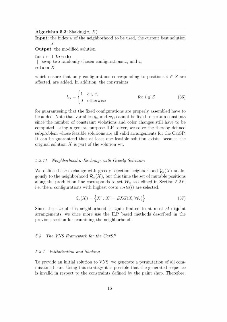
Algorithm 5.3: Shaking(u, X)

Input: the index u of the neighborhood to be used, the current best solutionX

Output: the modified solution

for i ← 1 to u doswap two randomly chosen configurations xi and xj

return X

which ensure that only configurations corresponding to positions i ∈ S areaffected, are added. In addition, the constraints

bci =

1 c ∈ xi

0 otherwisefor i 6∈ S (36)

for guaranteeing that the fixed configurations are properly assembled have tobe added. Note that variables gci and wfi cannot be fixed to certain constantssince the number of constraint violations and color changes still have to becomputed. Using a general purpose ILP solver, we solve the thereby definedsubproblem whose feasible solutions are all valid arrangements for the CarSP.It can be guaranteed that at least one feasible solution exists, because theoriginal solution X is part of the solution set.

5.2.11 Neighborhood κ-Exchange with Greedy Selection

We define the κ-exchange with greedy selection neighborhood Gκ(X) analo-gously to the neighborhood Rκ(X), but this time the set of mutable positionsalong the production line corresponds to set Wκ as defined in Section 5.2.6,i.e. the κ configurations with highest costs costs(i) are selected:

Gκ(X) ={

X ′ : X ′ = EXG(X,Wκ)}

(37)

Since the size of this neighborhood is again limited to at most κ! disjointarrangements, we once more use the ILP based methods described in theprevious section for examining the neighborhood.

5.3 The VNS Framework for the CarSP

5.3.1 Initialization and Shaking

To provide an initial solution to VNS, we generate a permutation of all com-missioned cars. Using this strategy it is possible that the generated sequenceis invalid in respect to the constraints defined by the paint shop. Therefore,

16

Table 1Order of the neighborhood structures for VND.

N1 = GS1 N4 = GSH5 N7 = SS2 N10 = SH N13 = R130

N2 = GSH1 N5 = GS20 N8 = S N11 = R65 N14 = G130

N3 = GS5 N6 = GSH20 N9 = SSH2 N12 = G65

we use a factor equal to n · |C| ·maxc∈C{γc} for penalizing each paint shop con-straint violation. In the further context we refer to this method for generatinginitial solutions as random arrangement (RA).

The shaking algorithm used for trying to escape local optima is straightfor-ward, see Alg. 5.3. Neighborhoods Nu(X), u = 1, . . . , umax, with umax = 3

4· n,

are implicitly defined by a series of u individual swaps of two randomly chosenconfigurations. Using this strategy has two advantages: firstly, evaluating andapplying swap moves can be done efficiently and secondly, diversification andtherefore the chance of escaping local optima grows with increasing values ofu.

5.3.2 The Order of the Neighborhoods for VND

Our implementation of VND applies tmax = 14 different neighborhood struc-tures N1, . . . ,N14. The order of these neighborhoods is crucial for runtimeperformance of the neighborhood search. Therefore, we decided to examinethem by increasing order of time complexity. Thus our VND implementationexplores the more expensive neighborhoods in the end. The order we used forour test runs is printed in Table 1.

In neighborhoods N1 to N6, we turn the attention on minimizing the maximumcontributions costs(i) to the objective function. The selection of the values forκ, i.e. κ = 1, 5, 20, is based on preliminary tests. If there was no improvementwithin these neighborhoods, we change our strategy for finding new and bettersolutions by trying to rearrange cars which are similar to each other (N7 andN9). To profit by exchanges of cars which are not very similar to each otherwe introduce neighborhoods N8 and N10. The neighborhoods based on swapmoves are examined first, because exploring them can be done faster thanevaluating neighborhoods utilizing shift moves. In the end the most expensiveneighborhoods based on κ-exchange moves are examined—once with 65 con-figurations set free and the second time with 130 cars to be rearranged. Thesevalues are chosen, because preliminary tests showed that problems of this sizecan be solved in acceptable time using exact methods based on integer linearprogramming.

17

5.3.3 Examining the Neighborhoods

For examining neighborhoods N1 to N10, we use two alternative strategies:best improvement and next improvement. For the remaining neighborhoodsN11 – N14, we use CPLEX 10.0 as general purpose ILP solver to solve theILP formulation presented in [12] to explore them. Analogously to best andnext improvement, we define a limited best improvement and a limited next

improvement strategy. Using limited next improvement the evaluation processterminates as soon as a better integer feasible solution was found or a timelimit has been reached. If no improvement could be achieved the best so farfound solution is returned.

6 Tests and Results

Two different sets of benchmark instances are considered here: the first onetaken from CSPlib [2] to compare our ILP approach with the one presentedby Gravel et al. in [4], and the second one taken from the instances provided byROADEF and the automobile manufacturer RENAULT for the ROADEF

Challenge 2005 [9] for testing our methods on larger instances. Only the latterinstances include constraints defined by the paint shop.

All experiments were performed on a dual AMD Opteron 2.4GHz PC with4GB RAM. Our algorithm has been implemented in C++ and for solving theILP formulations the general purpose ILP solver CPLEX 10.0 by ILOG hasbeen used.

6.1 Results on CSPlib Instances

The CSPlib library itself is split into two subsets of instances. The first onecontains 70 instances which are all satisfiable, i.e. there exists an optimalsolution with zero costs. All of these instances consist of exactly 200 cars with5 different components and 17 to 30 configurations. They are grouped intoseven classes, each of them indicating the utilization rate of the componentsin the instances, i.e. the percentage of cars requiring a component in regardto all cars of the instance. Each class has ten members and we refer to eachof these groups as util-rate-*, e.g. 60-* for the group of instances with anutilization rate of 60%.

The second subset of CSPlib benchmarks consists of nine additional instanceswhich are partly not completely satisfiable and typically harder to solve. Theseinstances consider 100 cars with 5 different components and 19 to 26 configu-

18

Table 2Average time for solving the CSPlib instances to optimality in seconds. Values inparentheses indicate standard deviation.

60-* 65-* 70-* 75-* 80-* 85-* 90-*

C-ILP 4.85 (5.8) 6.65 (5.4) 6.65 (1.7) 13.16 (8.4) 18.65 (10.6) 18.53 (8.7) 33.63 (15.1)

K-ILP 9.38 (6.0) 9.20 (5.1) 15.6 (3.6) 22.0 (12.5) 30.43 (12.0) 37.30 (13.7) 61.03 (26.1)

GRAVEL 3.27 (2.4) 6.87 (3.5) 11.94 (5.5) 15.85 (7.6) 27.86 (16.1) 40.39 (22.1) 77.26 (36.4)

1.7 (1.7) 3.1 (12.1) 8.6 (39.1) 3.1 (3.8) 4.5 (6.7) 14.6 (45.0) 40.2 (81.7)hybr. 98 99 94 93 93 97 93

1.2 (0.6) 1.3 (0.7) 1.5 (0.6) 1.8 (0.7) 2.5 (0.9) 2.9 (1.2) 3.6 (1.2)NA

heur. 85 86 88 78 66 43 10

0.6 (0.4) 0.6 (0.3) 0.9 (0.8) 2.8 (16.0) 6.5 (26.2) 4.9 (10.5) 10.3 (23.7)hybr. 100 100 99 98 96 97 93

0.5 (0.2) 0.6 (0.3) 0.6 (0.3) 1.0 (0.3) 1.4 (0.4) 1.6 (0.6) 2.1 (0.6)

bes

tR

A

heur. 98 97 90 85 60 45 16

0.9 (1.0) 1.4 (2.5) 2.0 (4.1) 2.2 (3.1) 8.5 (22.4) 7.6 (25.7) 27.7 (72.0)hybr. 100 100 100 98 100 98 96

0.8 (0.5) 0.8 (0.4) 1.0 (0.4) 1.3 (0.6) 2.1 (0.7) 2.2 (0.9) 3.0 (1.0)NA

heur. 91 90 89 80 60 42 16

0.7 (2.5) 0.6 (0.7) 0.9 (1.2) 1.6 (2.4) 5.9 (14.9) 6.0 (29.3) 11.9 (27.2)hybr. 100 100 100 100 98 99 99

0.4 (0.2) 0.5 (0.2) 0.6 (0.2) 0.8 (0.3) 1.2 (0.4) 1.4 (0.5) 1.7 (0.5)

nex

tR

A

heur. 94 91 94 80 57 42 18

rations.

Table 2 shows the results obtained for the test runs on the first subset ofCSPlib instances. The first three rows represent the mean time for each classneeded by the three ILP based exact approaches for finding optimal solutions(including proofs of optimality). The values in parentheses stand for the corre-sponding standard deviations. The second part of the table depicts the resultsobtained using the heuristic approaches. Each line contains the mean time forreaching the optimum, the corresponding standard deviation in parenthesesand below these two values the number of runs reaching the optimal solu-tion with zero costs. For the heuristic approaches ten runs per instance wereperformed. Therefore each mean value corresponds to 100 individual runs.

We refer with C-ILP to the ILP formulation presented in Section 4. K-ILP

stands for the formulation presented in [12] and GRAVEL denotes the resultsobtained by using the formulation by Gravel et al. [4]. Since this formulationuses a method of counting constraint violations different to the strategy pro-posed for the ROADEF Challenge 2005, we adapted their objective functionsuch that beside the number of positions with constraint violations the exactnumber of constraint violations is counted. In addition, we added a methodanalogously to the method presented in Section 4 for counting the numberof color changes. Finally, the weighted sum of all constraint violations andthe number of color changes is computed, see [11] for details. We indicate theresults obtained by using our VNS approach with (limited) best improvementwith best, whereas next denotes the setting with (limited) next improvement

19

used as step function for examining the neighborhoods.

To elaborate the impact of hybrid neighborhoods on the final results, we testedour approach using two different settings: The first one is based on the VNS-framework including all neighborhoods as described in Section 5 (we denotethis setting by hybr.) and the other one uses the same neighborhoods exceptthose taking advantage of the ILP based methods for examining them (denotedwith heur.).

Since our VNS approach did not yield promising results within preliminarytests for some instances using random arrangement (RA) for generating initialsolutions, we implemented a second method to which we refer as naive arrange-ment (NA). NA builds a sequence in a greedy way by placing all cars withconfiguration k1 ∈ K at the beginning, followed by cars with configurationk2 ∈ K and so on.

To summarize, the ILP formulation presented in Section 4 is in general thefastest one on these kind of instances. Since each of the instances can be solvedwithout any constraint violations and the objective function of the ILP formu-lations includes no negative terms, the corresponding LP relaxation triviallyis 0. Therefore, CPLEX consumes no extra time for proving optimality. Fur-thermore, as soon as our VNS approach reaches an objective value of 0, anoptimal solution is found. Thus, the comparison of run times given in Table 2is fair.

For the heuristic approaches, the hybrid VNS-approach yields better resultsthan the purely heuristic one with a forfeit of computation time across theboard. Further, the (limited) next improvement strategy provides faster atleast as good results than using (limited) best improvement as step functionand the initial solution generated by RA seems to have a positive impact onthe solution process for these instances. In general, the VNS-approaches areusually significantly faster than the exact methods with the drawback thatsometimes the optimal solution might not be reached.

For the second subset of CSPlib not all instances are satisfiable. Therefore,the first row of Table 3 covers the so far best known (and partly optimal)solution. The next three rows indicate the objective values obtained by solvingthe ILP models. Underneath these values the consumed computation times areprinted, whereas the solution process was stopped after 600 seconds and theso far best solution was used. The remaining eight rows reproduce the resultsobtained using the VNS approaches, where the average number of violationsover 10 runs, the standard deviation in parentheses and below these valuesthe total number of runs finding the best known solutions are printed for eachinstance and test setting.

The time needed for solving the ILP model as proposed in Section 4 is in

20

Table 3Computational results for the set of hard CSPlib instances. The first three rowspresent the results obtained by the exact methods whereas the remaining rows givean overview over results gained by the VNS approach.

10-93 16-81 19-71 21-90 26-82 36-92 41-66 4-72 6-76

best sol. 3 0 2 2 0 2 0 0 6

8 0 2 2 0 2 0 0 6C-ILP600.0 s 51.9 s 600.0 s 600.0 s 28.8 s 600.0 s 11.9 s 24.1 s 600.0 s

11 0 4 2 0 7 0 0 6K-ILP600.0 s 280.6 s 600.0 s 600.0 s 23.0 s 600.0 s 13.0 s 35.6 s 600.0 s

6 0 3 4 0 2 0 0 6GRAVEL600.0 s 49.4 s 600.0 s 600.0 s 32.1 s 600.0 s 14.5 s 41.4 s 600.0 s

16.7 (6.0) 19.6 (7.0) 9.5 (4.7) 4.1 (4.6) 3.4 (5.7) 9.4 (2.9) 0.0 (0.0) 7.9 (6.5) 7.3 (1.8)hybr. 0 0 1 8 6 0 10 1 4

25.9 (2.6) 24.8 (2.8) 17.1 (3.0) 15.2 (2.6) 12.4 (4.2) 17.3 (2.1) 6.9 (1.7) 15.4 (2.7) 12.0 (2.1)NA

heur. 0 0 0 0 0 0 0 0 0

18.3 (5.0) 18.7 (5.5) 8.4 (5.0) 3.4 (2.4) 4.9 (5.2) 8.7 (1.5) 0.9 (2.0) 9.3 (5.5) 7.3 (1.4)hybr. 0 0 1 7 4 0 8 1 4

26.5 (3.5) 22.6 (4.4) 15.9 (3.2) 12.7 (2.5) 13.2 (3.3) 15.2 (2.4) 7.7 (1.4) 15.1 (2.1) 11.8 (1.0)

bes

tR

A

heur. 0 0 0 0 0 0 0 0 0

7.1 (1.4) 0.0 (0.0) 3.5 (1.5) 3.1 (1.4) 0.0 (0.0) 3.9 (0.7) 0.0 (0.0) 0.0 (0.0) 6.0 (0.0)hybr. 0 10 2 3 10 0 10 10 10

25.9 (2.8) 22.8 (3.8) 18.3 (3.8) 14.3 (2.3) 13.4 (4.5) 15.8 (2.6) 6.5 (1.5) 14.8 (2.4) 11.0 (1.3)NA

heur. 0 0 0 0 0 0 0 0 0

8.0 (1.1) 0.0 (0.0) 3.2 (1.2) 3.0 (0.9) 0.0 (0.0) 3.7 (1.4) 0.0 (0.0) 0.2 (0.6) 6.0 (0.0)hybr. 0 10 3 3 10 2 10 9 10

25.2 (2.7) 20.7 (3.5) 18.0 (2.5) 12.8 (2.1) 11.6 (2.5) 16.4 (3.1) 8.0 (2.0) 15.9 (1.4) 11.4 (1.6)

nex

tR

A

heur. 0 0 0 0 0 0 0 0 0

general shorter than the computation time needed for solving the model in-troduced by Gravel et al. [4]. Is is evident that the third formulation is theworst one on these instances. Results obtained for the VNS approaches aresimilar to the previously presented results. On this second subset of CSPlib

instances the hybrid approach is much better than the pure heuristic one,which was not able to find the best known solution for any of the instances.Again, the (limited) next improvement strategy yields better results in shortertime than (limited) best improvement and the strategy for generating an initialsolution seems to have no noticeable impact on the solution process.

In conclusion, the hybrid VNS approach with (limited) next improvementas step function and RA used for generating initial solutions yields the bestresults on CSPlib instances. The results obtained using the hybrid variantsof the VNS approach justify the extra computation time needed during thesolution process. For the second subset of instances the traditional approachwas even not able to reach the so far best known solution for any instance.The high performance of (limited) next improvement in contrast to (limited)best improvement can be explained by the extra time available for additionalVNS iterations, because especially in the large neighborhoods examined usingILP based methods much time is consumed for trying to prove optimality for

21

a found solution.

6.2 ROADEF instances

ROADEF and the automobile manufacturer RENAULT published threesets of test instances for the ROADEF Challenge 2005: set A, B, and X [9].We used set X for the experiments documented here, since this set was alsoused for the final evaluation procedure and ranking of the candidates. Thereare 19 instances with 65 to 1319 cars, 5 to 20 colors, 5 to 26 components,and 10 to 328 configurations in set X. For the final evaluation process atthe ROADEF Challenge 2005 the available computation time was limited to600 seconds on a Pentium IV 1.6 GHz with 1 GB RAM. Since the objectivefunction defined by RENAULT for the ROADEF Challenge 2005 is slightlydifferent from function (1) stated previously, the number of violations whichdefinitely occur at the first positions of the production of the next day areadded to the objective function for these tests.

Although the ILP formulation presented in Section 4 yields good results onCSPlib instances, preliminary tests showed that the formulation presentedin [12] yields faster at least as good results on instances including paint shopconstraints. Therefore, we used this formulation for examining large neighbor-hoods.

Each column in Tables 4 and 5 represents one instance from set X. In the head-ing, the instance number, the number of cars, the number of components, andthe number of colors are presented. Rows 1 to 8 show average results for eachinstance over ten runs using 600 seconds as time limit. The values beneaththe averages indicate the standard deviations. A triple of values v1/v2/v3 in-dicates v1 violations of the highest order objective, v2 violations of the secondobjective and v3 violations of the least important objective. Again best/next

represents the step function used, NA/RA denotes the strategy for generat-ing the initial solution and hybr./heur. indicates which sets of neighborhoodshave been used for the test runs. The two rows labeled with R-best and R-

worst indicate the objective value of the best and worst solution among thecandidates obtained during the final evaluation procedure of the ROADEF

Challenge 2005, respectively. The last three rows present results obtained bysolving the instances using the different ILP formulations. Cells without anyentry indicate that even solving the LP-relaxations for these instances was notpossible within the given time limits. If one entry is given, this value representsa lower bound on the corresponding instance. If two values are printed in onecell, there are two possibilities: the first one indicates an upper and a lowerbound for the optimum. The other value indicates the objective value of theoptimum and the solution time in seconds (including the proof of optimality)

22

Table 4. Results obtained for set X of the ROADEF Challenge 2005. The first eight rows represent the objective values (and standarddeviations below) obtained using different settings of the VNS approach. The next 2 lines represent the best and worst results obtainedduring the ROADEF Challenge 2005, respectively. The last three rows indicate the results obtained using CPLEX solving the discussedILP models.

inst. n (1) 704 (2) 1260 (3) 1319 (4) 996 (5) 325 (6) 65 (7) 780 (8) 921 (9) 231 (10) 90|C| |F | 12 13 12 13 18 15 20 20 26 15 6 5 7 14 8 10 7 8 1 6

13.0/2.1/4.6 0.0/260.4/57.4 80.0/537.4/61.1 5.5/329.7/637.3 46.5/429.3/ 99.8 0.0/0.0/3.0 0.0/181.2/ 12.3 0.0/116.1/599.3 8.8/ 95.1/49.9 5.7/10.3/0.0hybr. 0.0/0.3/1.6 0.0/ 5.7/ 7.1 8.3/ 12.4/13.8 4.2/ 25.9/ 8.0 2.6/ 11.6/ 4.6 0.0/0.0/0.0 0.0/ 8.4/ 11.0 0.0/ 6.8/ 23.2 1.7/ 1.4/ 7.0 0.5/ 0.5/0.0

13.0/4.8/9.2 0.0/257.0/64.7 79.3/542.3/61.7 4.5/310.3/636.5 49.7/447.6/ 98.1 0.0/0.0/4.0 0.0/186.6/ 14.1 0.0/117.0/605.7 11.3/102.5/54.2 6.0/11.0/0.0NA

heur. 0.0/0.4/1.8 0.0/ 3.5/ 9.4 11.7/ 9.9/22.2 5.4/ 18.0/ 10.7 4.5/ 13.0/ 2.9 0.0/0.0/0.0 0.0/ 6.1/ 9.9 0.0/ 11.5/ 21.6 2.8/ 3.1/ 9.2 0.0/ 0.0/0.0

111.5/0.2/0.6 0.0/394.1/40.1 67.8/573.5/37.3 10.7/312.9/648.4 46.0/425.3/ 96.2 0.0/0.0/3.1 0.0/213.8/ 7.3 0.0/219.1/491.0 8.6/ 95.5/45.6 6.5/10.4/0.0hybr. 7.4/0.6/1.1 0.0/ 7.1/ 4.4 6.2/ 8.9/14.0 3.6/ 20.6/ 10.8 3.6/ 14.4/ 2.9 0.0/0.0/0.3 0.0/ 12.1/ 9.8 0.0/ 8.2/ 8.4 1.1/ 2.1/ 6.8 1.6/ 0.5/0.0

170.3/0.3/0.5 0.0/398.0/41.6 68.6/570.1/34.1 10.3/302.3/640.5 49.2/448.2/ 96.6 0.0/0.0/4.3 0.0/218.5/ 5.5 0.0/230.1/491.9 11.5/107.2/37.1 16.8/10.9/0.0

bes

t

RA

heur. 11.2/0.7/0.8 0.0/ 10.1/ 8.3 8.2/ 13.4/11.5 4.0/ 15.4/ 11.1 3.1/ 12.9/ 4.0 0.0/0.0/0.5 0.0/ 12.2/ 2.4 0.0/ 5.9/ 8.4 2.5/ 2.9/ 4.1 3.6/ 0.9/0.0

13.0/2.0/8.5 0.0/330.3/44.5 78.0/562.2/39.1 6.4/353.9/637.6 44.2/428.9/ 96.6 0.0/0.0/3.0 0.0/181.2/ 7.0 0.0/175.4/506.0 8.9/ 95.7/43.6 5.2/10.8/0.0hybr. 0.0/0.0/2.5 0.0/ 11.7/ 7.9 8.2/ 16.0/13.3 3.3/ 36.8/ 8.7 1.8/ 11.4/ 2.6 0.0/0.0/0.0 0.0/ 8.4/ 6.4 0.0/ 10.5/ 9.3 2.2/ 2.3/ 5.2 0.4/ 0.4/0.0

13.0/3.3/9.6 0.0/335.8/43.8 83.5/566.3/37.9 6.5/359.5/643.0 45.9/450.2/ 97.9 0.0/0.0/4.1 0.0/184.6/ 4.9 0.0/176.4/514.9 12.7/106.9/44.8 6.0/11.0/0.0NA

heur. 0.0/1.1/3.6 0.0/ 7.9/ 5.9 12.0/ 21.5/13.9 2.0/ 45.4/ 10.1 3.2/ 13.2/ 3.7 0.0/0.0/0.3 0.0/ 7.2/ 3.4 0.0/ 6.7/ 8.8 3.2/ 3.2/10.2 0.0/ 0.0/0.0

85.0/0.5/1.8 0.0/376.3/42.2 81.6/578.0/31.1 8.8/349.2/634.2 45.5/434.0/ 98.9 0.0/0.0/3.0 0.0/195.4/ 3.5 0.0/206.7/484.7 8.6/ 94.7/44.8 5.5/10.7/0.0hybr. 11.8/0.8/1.2 0.0/ 10.8/ 4.4 6.5/ 13.5/ 5.3 3.1/ 15.5/ 15.7 4.1/ 18.9/ 3.6 0.0/0.0/0.0 0.0/ 5.9/ 1.1 0.0/ 4.4/ 8.0 1.9/ 1.2/ 5.5 1.1/ 0.5/0.0

139.7/0.8/0.9 0.0/387.4/44.2 69.2/582.9/34.2 7.9/345.1/638.4 45.6/448.1/ 97.7 0.0/0.0/4.4 0.0/198.2/ 3.0 0.0/215.2/499.1 10.8/106.9/42.2 15.9/10.5/0.0

nex

t

RA

heur. 14.2/1.0/1.1 0.0/ 6.2/ 6.5 8.2/ 22.2/12.9 4.7/ 31.6/ 11.5 3.2/ 11.4/ 4.2 0.0/0.0/0.5 0.0/ 9.3/ 0.9 0.0/ 7.2/ 9.3 2.2/ 2.1/ 8.0 1.9/ 0.7/0.0

R-best 12.0/2.0/3.0 0.0/192.4/66.0 0.0/337.0/ 6.0 0.0/160.0/407.6 36.0/341.4/ 95.4 0.0/0.0/3.0 0.0/110.2/ 98.4 0.0/ 55.2/794.8 8.0/ 35.8/87.0 5.0/10.0/0.0

R-worst 12.2/2.0/4.4 0.0/314.0/44.0 49.4/444.8/33.8 16.0/950.0/509.0 338.2/408.0/118.2 0.0/9.4/3.0 0.0/180.8/223.8 0.0/145.0/530.0 12.0/103.0/52.0 6.0/10.0/0.0

– – – – – 0.0/0.0/3.0 – – – 5.0/10.0/0.0C-ILP

– – – – – 0.33 s – – 1 001 501.0 18.98 s

– – – – – 3.0 – – – 5.0/10.0/0.0K-ILP

– – – – – 0.25 s – – 1 001 501.0 48.38 s

– – – – – 3.0 – – – 7 012 000.0GRAVEL

– – – – – 17.98 s – – 1 001 023.0 1 552 111.0

23

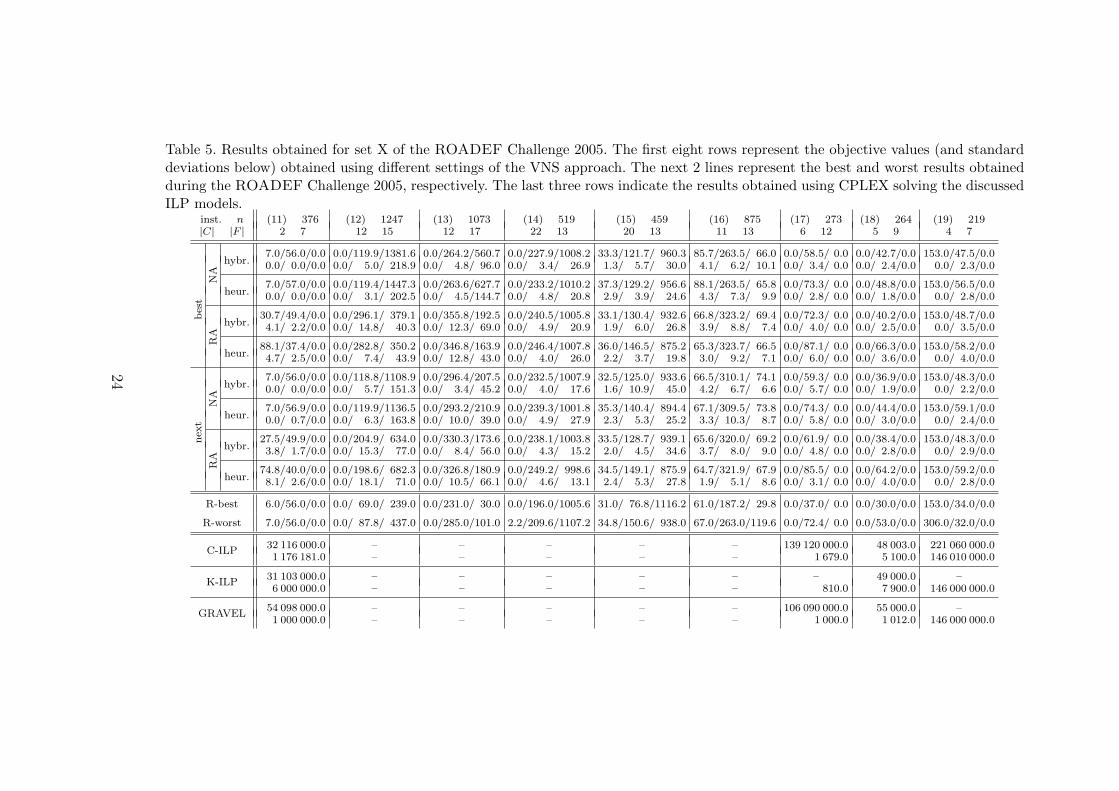
Table 5. Results obtained for set X of the ROADEF Challenge 2005. The first eight rows represent the objective values (and standarddeviations below) obtained using different settings of the VNS approach. The next 2 lines represent the best and worst results obtainedduring the ROADEF Challenge 2005, respectively. The last three rows indicate the results obtained using CPLEX solving the discussedILP models.

inst. n (11) 376 (12) 1247 (13) 1073 (14) 519 (15) 459 (16) 875 (17) 273 (18) 264 (19) 219|C| |F | 2 7 12 15 12 17 22 13 20 13 11 13 6 12 5 9 4 7

7.0/56.0/0.0 0.0/119.9/1381.6 0.0/264.2/560.7 0.0/227.9/1008.2 33.3/121.7/ 960.3 85.7/263.5/ 66.0 0.0/58.5/ 0.0 0.0/42.7/0.0 153.0/47.5/0.0hybr. 0.0/ 0.0/0.0 0.0/ 5.0/ 218.9 0.0/ 4.8/ 96.0 0.0/ 3.4/ 26.9 1.3/ 5.7/ 30.0 4.1/ 6.2/ 10.1 0.0/ 3.4/ 0.0 0.0/ 2.4/0.0 0.0/ 2.3/0.0

7.0/57.0/0.0 0.0/119.4/1447.3 0.0/263.6/627.7 0.0/233.2/1010.2 37.3/129.2/ 956.6 88.1/263.5/ 65.8 0.0/73.3/ 0.0 0.0/48.8/0.0 153.0/56.5/0.0NA

heur. 0.0/ 0.0/0.0 0.0/ 3.1/ 202.5 0.0/ 4.5/144.7 0.0/ 4.8/ 20.8 2.9/ 3.9/ 24.6 4.3/ 7.3/ 9.9 0.0/ 2.8/ 0.0 0.0/ 1.8/0.0 0.0/ 2.8/0.0

30.7/49.4/0.0 0.0/296.1/ 379.1 0.0/355.8/192.5 0.0/240.5/1005.8 33.1/130.4/ 932.6 66.8/323.2/ 69.4 0.0/72.3/ 0.0 0.0/40.2/0.0 153.0/48.7/0.0hybr. 4.1/ 2.2/0.0 0.0/ 14.8/ 40.3 0.0/ 12.3/ 69.0 0.0/ 4.9/ 20.9 1.9/ 6.0/ 26.8 3.9/ 8.8/ 7.4 0.0/ 4.0/ 0.0 0.0/ 2.5/0.0 0.0/ 3.5/0.0

88.1/37.4/0.0 0.0/282.8/ 350.2 0.0/346.8/163.9 0.0/246.4/1007.8 36.0/146.5/ 875.2 65.3/323.7/ 66.5 0.0/87.1/ 0.0 0.0/66.3/0.0 153.0/58.2/0.0

bes

t

RA

heur. 4.7/ 2.5/0.0 0.0/ 7.4/ 43.9 0.0/ 12.8/ 43.0 0.0/ 4.0/ 26.0 2.2/ 3.7/ 19.8 3.0/ 9.2/ 7.1 0.0/ 6.0/ 0.0 0.0/ 3.6/0.0 0.0/ 4.0/0.0

7.0/56.0/0.0 0.0/118.8/1108.9 0.0/296.4/207.5 0.0/232.5/1007.9 32.5/125.0/ 933.6 66.5/310.1/ 74.1 0.0/59.3/ 0.0 0.0/36.9/0.0 153.0/48.3/0.0hybr. 0.0/ 0.0/0.0 0.0/ 5.7/ 151.3 0.0/ 3.4/ 45.2 0.0/ 4.0/ 17.6 1.6/ 10.9/ 45.0 4.2/ 6.7/ 6.6 0.0/ 5.7/ 0.0 0.0/ 1.9/0.0 0.0/ 2.2/0.0

7.0/56.9/0.0 0.0/119.9/1136.5 0.0/293.2/210.9 0.0/239.3/1001.8 35.3/140.4/ 894.4 67.1/309.5/ 73.8 0.0/74.3/ 0.0 0.0/44.4/0.0 153.0/59.1/0.0NA

heur. 0.0/ 0.7/0.0 0.0/ 6.3/ 163.8 0.0/ 10.0/ 39.0 0.0/ 4.9/ 27.9 2.3/ 5.3/ 25.2 3.3/ 10.3/ 8.7 0.0/ 5.8/ 0.0 0.0/ 3.0/0.0 0.0/ 2.4/0.0

27.5/49.9/0.0 0.0/204.9/ 634.0 0.0/330.3/173.6 0.0/238.1/1003.8 33.5/128.7/ 939.1 65.6/320.0/ 69.2 0.0/61.9/ 0.0 0.0/38.4/0.0 153.0/48.3/0.0hybr. 3.8/ 1.7/0.0 0.0/ 15.3/ 77.0 0.0/ 8.4/ 56.0 0.0/ 4.3/ 15.2 2.0/ 4.5/ 34.6 3.7/ 8.0/ 9.0 0.0/ 4.8/ 0.0 0.0/ 2.8/0.0 0.0/ 2.9/0.0

74.8/40.0/0.0 0.0/198.6/ 682.3 0.0/326.8/180.9 0.0/249.2/ 998.6 34.5/149.1/ 875.9 64.7/321.9/ 67.9 0.0/85.5/ 0.0 0.0/64.2/0.0 153.0/59.2/0.0

nex

t

RA

heur. 8.1/ 2.6/0.0 0.0/ 18.1/ 71.0 0.0/ 10.5/ 66.1 0.0/ 4.6/ 13.1 2.4/ 5.3/ 27.8 1.9/ 5.1/ 8.6 0.0/ 3.1/ 0.0 0.0/ 4.0/0.0 0.0/ 2.8/0.0

R-best 6.0/56.0/0.0 0.0/ 69.0/ 239.0 0.0/231.0/ 30.0 0.0/196.0/1005.6 31.0/ 76.8/1116.2 61.0/187.2/ 29.8 0.0/37.0/ 0.0 0.0/30.0/0.0 153.0/34.0/0.0

R-worst 7.0/56.0/0.0 0.0/ 87.8/ 437.0 0.0/285.0/101.0 2.2/209.6/1107.2 34.8/150.6/ 938.0 67.0/263.0/119.6 0.0/72.4/ 0.0 0.0/53.0/0.0 306.0/32.0/0.0

32 116 000.0 – – – – – 139 120 000.0 48 003.0 221 060 000.0C-ILP

1 176 181.0 – – – – – 1 679.0 5 100.0 146 010 000.0

31 103 000.0 – – – – – – 49 000.0 –K-ILP

6 000 000.0 – – – – – 810.0 7 900.0 146 000 000.0

54 098 000.0 – – – – – 106 090 000.0 55 000.0 –GRAVEL

1 000 000.0 – – – – – 1 000.0 1 012.0 146 000 000.0

24

Table 6Mapping of short names to names used by ROADEF and RENAULT for theROADEF Challenge 2005.

short name original name # cars # components # colors

(1) 022 RAF EP ENP S49 J2 704 12 13

(2) 023 EP RAF ENP S49 J2 1260 12 13

(3) 024 EP RAF ENP S49 J2 1319 18 15

(4) 025 EP ENP RAF S49 J1 996 20 20

(5) 028 CH1 EP ENP RAF S50 J4 325 26 15

(6) 028 CH2 EP ENP RAF S51 J1 65 6 5

(7) 029 EP RAF ENP S49 J5 780 7 14

(8) 034 VP EP RAF ENP S51 J1 J2 J3 921 8 10

(9) 034 VU EP RAF ENP S51 J1 J2 J3 231 7 8

(10) 035 CH1 RAF EP S50 J4 90 1 6

(11) 035 CH2 RAF EP S50 J4 376 2 7

(12) 039 CH1 EP RAF ENP S49 J1 1247 12 15

(13) 039 CH3 EP RAF ENP S49 J1 1073 12 17

(14) 048 CH1 EP RAF ENP S50 J4 519 22 13

(15) 048 CH2 EP RAF ENP S49 J5 459 20 13

(16) 064 CH1 EP RAF ENP S49 J1 875 11 13

(17) 064 CH2 EP RAF ENP S49 J4 273 6 12

(18) 655 CH1 EP RAF ENP S51 J2 J3 J4 264 5 9

(19) 655 CH2 EP RAF ENP S52 J1 J2 S01 J1 219 4 7

labeled with s. A mapping of the names used in Tables 4–5 to the originalnames as used by ROADEF and RENAULT can be found in Table 6.

Referring to Table 4 and 5, it can be seen that for instances 6 and 10 we wereable to find best solutions and prove their optimality using the exact methodsbased on integer linear programming. Further, we were able to compute lowerbounds for instances 11 and 19 which indicate that the currently known bestsolution is close to the optimum.

In general, the instances proposed for the ROADEF Challenge 2005 are toolarge to be solved exactly. Even computing the LP-relaxations of currentlyavailable ILP formulations for ROADEF instances is in general too expensivein practice. The VNS approach proposed in this paper provides competitiveresults in comparison with the best methods of the challenge. Especially thecombination of the VNS scheme with the exact ILP approach for searchinglarge neighborhoods leads to excellent results in comparison with the pureheuristic VNS approach.

We further studied the individual contributions of each neighborhood duringa run of VNS. Figure 4 exemplarily shows for instance 15 measured improve-ment ratios, i.e. the ratios of neighborhood evaluations yielding improved so-lutions to the total number of evaluations. The first plot are the results for

25

Fig. 4. This plot presents a characteristic graphical output of statistics indicatingthe ratio of improvements and total searches in the individual neighborhoods.

the hybrid approach with (limited) best strategy and NA for generating ini-tial solutions. The second plot show ratios obtained by using the same settingbut without those neighborhoods examined using ILP based methods. Theseresults—together with those presented in Table 4—verify that examining theneighborhoods examined using ILP based methods is beneficial and can im-prove the final results after 600 seconds CPU time.

It is interesting that the approaches using NA yield better results than theapproaches using RA for generating initial solutions for 14 out of 19 ROADEFinstances. This happens, because initial solutions generated by NA are mostlyinfeasible, since the constraints defined by the paint shop are violated in gen-eral. Therefore, the first iterations of VND are typically used for repairingthese solutions with respect to these constraints. However, once such a so-lution is feasible with respect to the paint shop constraints, it will usuallycontain substantially fewer color changes than a random solution derived byRA. In the further optimization, it seems to be hard for the VNS to make largeimprovements with respect to the number of color changes, while focusing atthe same time on the other objective of reducing lc/mc constraint violations.

We were not able to notice a significant performance difference between (lim-ited) best and next improvement, although a trend towards (limited) nextimprovement being more promising can be detected.

7 Conclusions

In this paper we presented an ILP formulation which can be used to solve in-stances with up to about 300 cars to proven optimality. On CSPlib instances,this formulation leads to significantly shorter computation time than compa-

26

rable formulations from literature. This in particular holds for instances withhigh utilization rates. For two ROADEF instances we were able to providenew optimality proofs for already known solutions and for two other instanceswe were able to compute tight lower bounds indicating that the currentlyknown best solution is close to the optimum.

Further, we presented a general variable neighborhood search approach tothe car sequencing problem, which takes advantage of by searching largeneighborhoods by means of integer linear programming. Since the considera-tion of these is beneficial but computationally expensive, we combined themwith traditional neighborhoods that can be quickly searched by enumeration.This approach is competitive compared to the methods presented during theROADEF Challenge 2005 and the variants of our VNS approach includingneighborhoods examined using ILP based methods outperform those variantswithout these neighborhoods.

For the future, we have plans to add and investigate further large neighborhoodstructures and other ILP techniques for searching them. For instance, it seemspromising to also consider Lagrangian relaxation based methods.

References

[1] I. P. Gent. Two results on car-sequencing problems. Technical report, APES-02-1998, Department of Computer Science, University of Strathclyde, UK, April1998.

[2] I. P. Gent and T. Walsh. CSPlib: a benchmark library for constraints.Technical report, APES-09-1999, Department of Computer Science, Universityof Strathclyde, UK, 1999.

[3] J. Gottlieb, M. Puchta, and C. Solnon. A study of greedy, local search, and antcolony optimization approaches for car sequencing problems. In G. R. Raidlet al., editors, Proceedings of the Applications of Evolutionary Computing onEvoWorkshops 2003, volume 2611 of Lecture Notes in Computer Science, pages246–257. Springer-Verlag Berlin Heidelberg, 2003.

[4] M. Gravel, C. Gagne, and W. L. Price. Review and comparison of three methodsfor the solution of the car sequencing problem. Journal of the OperationalResearch Society, 56(11):1287–1295, November 2005.

[5] P. Hansen and N. Mladenovic. A tutorial on variable neighborhood search.Technical Report G-2003-46, Les Cahiers du GERAD, HEC Montreal andGERAD, Canada, 2003.

[6] B. Hu. Interaktive Reihenfolgeplanung fur die Automobilindustrie. Master’sthesis, Vienna University of Technology, Vienna, Austria, 2004.

27

[7] A. Jaszkiewicz, P. Kominek, and M. Kubiak. Adaptation of the genetic localsearch algorithm to a car sequencing problem. 7th National Conference onEvolutionary Algorithms and Global Optimization, Kazimierz Dolny, Poland,pages 67–74, 2004.

[8] T. Kis. On the complexity of the car sequencing problem. Operations ResearchLetters, 32(4):331–335, July 2004.

[9] A. Nguyen. Challenge ROADEF’2005: Car sequencing problem. online referenceat http://www.prism.uvsq.fr/~vdc/ROADEF/CHALLENGES/2005/. last visitedOctober 31, 2006.

[10] L. Perron and P. Shaw. Combining forces to solve the car sequencing problem.In J.-C. Regin and M. Rueher, editors, CPAIOR, volume 3011 of Lecture Notesin Computer Science, pages 225–239. Springer, 2004.

[11] M. Prandtstetter. Exact and heuristic methods for solving the Car SequencingProblem. Master’s thesis, Vienna University of Technology, Vienna, Austria,2005.

[12] M. Prandtstetter and G. R. Raidl. A variable neighborhood search approach forsolving the car sequencing problem. In Proceedings of the XVIII Mini EUROConference on VNS, Tenerife, Spain, 2005.

[13] M. Puchta and J. Gottlieb. Solving car sequencing problems by localoptimization. In Proceedings of the Applications of Evolutionary Computingon EvoWorkshops 2002, volume 2279 of Lecture Notes in Computer Science,pages 132–142, London, UK, 2002. Springer-Verlag.

28