An Integer Programming Approach for

Linear Programs with Probabilistic Constraints ∗†

James LuedtkeShabbir Ahmed

George NemhauserGeorgia Institute of Technology

765 Ferst Drive, Atlanta, GA, USAluedtke@gatech.edu

May 3, 2007

Abstract

Linear programs with joint probabilistic constraints (PCLP) are dif-ficult to solve because the feasible region is not convex. We consider aspecial case of PCLP in which only the right-hand side is random andthis random vector has a finite distribution. We give a mixed-integerprogramming formulation for this special case and study the relaxationcorresponding to a single row of the probabilistic constraint. We obtaintwo strengthened formulations. As a byproduct of this analysis, we obtainnew results for the previously studied mixing set, subject to an additionalknapsack inequality. We present computational results which indicatethat by using our strengthened formulations, instances that are consider-ably larger than have been considered before can be solved to optimality.

Keywords: Stochastic Programming, Integer Programming, Probabilistic Con-straints, Chance Constraints, Mixing Set

1 Introduction

Consider a linear program with a probabilistic or chance constraint

(PCLP ) min{

cx : x ∈ X, P{Tx ≥ ξ} ≥ 1 − ǫ}

(1)

∗This research has been supported in part by the National Science Foundation under grantsDMI-0121495 and DMI-0522485.

†An extended abstract of this paper has been published in the Proceedings of the TwelfthConference on Integer Programming and Combinatorial Optimization (IPCO 2007) [13].

1

where X ={

x ∈ Rd+ : Ax = b

}

is a polyhedron, c ∈ Rd, T is an m × d random

matrix, ξ is a random vector taking values in Rm, and ǫ is a confidence parameter

chosen by the decision maker, typically near zero, e.g., ǫ = 0.01 or ǫ = 0.05. Notethat in (1) we enforce a single probabilistic constraint over all rows, rather thanrequiring that each row independently be satisfied with high probability. Sucha constraint is known as a joint probabilistic constraint, and is appropriate in acontext in which it is important to have all constraints satisfied simultaneouslyand there may be dependence between random variables in different rows.

Problems with joint probabilistic constraints have been extensively studied;see [17] for background and an extensive list of references. Probabilistic con-straints have been used in various applications including supply chain manage-ment [11], production planning [15], optimization of chemical processes [9, 10]and surface water quality management [20]. Unfortunately, linear programswith probabilistic constraints are still largely intractable except for a few veryspecial cases. There are two primary reasons for this intractability. First, ingeneral, for a given x ∈ X , the quantity P{Tx ≥ ξ} is hard to compute, as itrequires multi-dimensional integration. Second, the feasible region defined by aprobabilistic constraint generally is not convex.

In this work, we demonstrate that by using integer programming techniques,instances of PCLP that are considerably larger than have been considered beforecan be solved to optimality under the following two simplifying assumptions:

(A1) Only the right-hand side vector ξ is random; the matrix T = T is deter-ministic.

(A2) The random vector ξ has a finite distribution.

Despite its restrictiveness, the special case given by assumption A1 has receivedconsiderable attention in the literature, see, e.g., [5, 6, 17]. A notable result forthis case is that if the distribution of the right-hand side is log-concave, then thefeasible region defined by the joint probabilistic constraint is convex [16]. Thisallows problems in which the dimension, m, of the random vector is small to besolved to optimality, but higher dimensional problems are still intractable due tothe difficulty in checking feasibility of the probabilistic constraint. Specializedmethods have been developed in [4, 6, 17] for the case in which assumption A1holds and the random vector has discrete but not necessarily finite distribution.These methods rely on the enumeration of certain efficient points of the distri-bution, and hence do not scale well with m since the number of efficient pointsgenerally grows exponentially with m.

Assumption A2 may also seem very restrictive. However, if the possiblevalues for ξ are generated by taking Monte Carlo samples from a general dis-tribution, we can think of the resulting problem as an approximation of theproblem with general distribution. Under some reasonable assumptions we canshow that the optimal solution of the sampled problem converges exponentiallyfast to the optimal solution of the original problem as the number of scenariosincreases. Also, the optimal objective of the sampled problem can be used to

2

develop statistical lower bounds on the optimal objective of the original prob-lem. See [1, 3, 19] for some related results. It seems that the reason such asampling approach has not been seriously considered for PCLP in the past isthat the resulting sampled problem has a non-convex feasible region, and thusis generally intractable. Our contribution is to demonstrate that, at least underassumption A1, it is nonetheless possible to solve the sampled problem.

Under assumption A2 it is possible to write a mixed-integer programming(MIP) formulation for PCLP, as has been done, for example, in [18]. In thegeneral case, such a formulation requires the introduction of “big-M” type con-straints, and hence is difficult to solve. However, by restricting attention to thecase of assumption A1, we are able to develop strong mixed-integer program-ming formulations. Our approach in developing these formulations is to considerthe relaxation obtained from a single row in the probabilistic constraint. Thisyields a system similar to the mixing set introduced by Gunluk and Pochet[8], subject to an additional knapsack inequality. We are able to derive strongvalid inequalities for this system by first using the knapsack inequality to “pre-process” the mixing set and then applying the mixing inequalities of [8]; seealso [2, 7]. We also derive an extended formulation, equivalent to one given byMiller and Wolsey in [14]. Making further use of the knapsack inequality, we areable to derive more general classes of valid inequalities for both the original andextended formulations. If all scenarios are equally likely, the knapsack inequal-ity reduces to a cardinality restriction. In this case, we are able to characterizethe convex hull of feasible solutions to the extended formulation for the singlerow case. Although these results are motivated by the application to PCLP,they can be used in any problem in which a mixing set appears along with aknapsack constraint.

The remainder of this paper is organized as follows. In Section 2 we verifythat PCLP remains NP -hard even under assumptions A1 and A2, and presentthe standard MIP formulation. In Section 3 we analyze this MIP and presentclasses of valid inequalities that make the formulation strong. In Section 4 wepresent an extended formulation, and a new class of valid inequalities and showthat in the equi-probable scenarios case, these inequalities define the convex hullof the single row formulation. In Section 5 we present computational resultsusing the strengthened formulations, and we close with concluding remarks inSection 6.

2 The MIP Formulation

We now consider a probabilistically constrained linear programming problemwith random right-hand side given by

(PCLPR) min cxs.t. Ax = b

P{Tx ≥ ξ} ≥ 1 − ǫx ≥ 0.

(2)

3

Here A is an r×d matrix, b ∈ Rr, T is an m×d matrix, ξ is a random vector in

Rm, ǫ ∈ (0, 1) (typically small) and c ∈ R

d. We assume that ξ has finite support,that is there exist vectors, ξi ∈ R

m, i = 1, . . . , n such that P{ξ = ξi} = πi foreach i where πi > 0 and

∑ni=1 πi = 1. We refer to the possible outcomes as

scenarios. We assume without loss of generality that ξi ≥ 0 and πi ≤ ǫ for eachi. We also define the set N = {1, . . . , n}.

Before proceeding, we note that PCLPR is NP-hard even under assumptionsA1 and A2.

Theorem 1. PCLPR is NP-hard, even in the special case in which πi = 1/nfor all i ∈ N , the constraints Ax = b are not present, T is the m × m identity

matrix, and c = (1, . . . , 1) ∈ Rm.

Proof. Let K = ⌈(1 − ǫ)n⌉. Then, under the stated conditions PCLPR can bewritten as

minI⊆N

m∑

j=1

maxi∈I

{ξij} : |I| ≥ K

.

We show that the associated decision problem:

(DPCLP) Given non-negative integers ξij for i = 1, . . . , n, j =1, . . . , m, K ≤ n and B, is there an I ⊆ N such that |I| ≥ Kand

∑mj=1 maxi∈I {ξij} ≤ B?

is NP-complete by reduction from the NP-complete problem CLIQUE. Consideran instance of CLIQUE given by graph G = (V, E), in which we wish to decidewhether there exists a clique of size C. We construct an instance of DPCLP byletting {1, . . . , m} = V , N = E, B = C, K = C(C − 1)/2 and ξij = 1 if edge iis incident to node j and ξij = 0 otherwise. The key observation is that for anyI ⊆ E, and j ∈ V ,

maxi∈I

{ξij} =

{

1 if some edge i ∈ I is incident to node j0 otherwise.

Hence, if there exists a clique of size C in G then we have a subgraph of Gconsisting of C nodes and C(C − 1)/2 edges. Thus there exists I ⊆ N with|I| = C(C − 1)/2 = K and

m∑

j=1

maxi∈I

{ξij} = C = B

and the answer to DPCLP is yes.Conversely, if the answer to DPCLP is yes, there exists I ⊆ E of size at least

K = C(C −1)/2 such that the number of nodes incident to I is at most B = C.This can only happen if I defines a clique of size C.

We now formulate PCLPR as a mixed-integer program [18]. To do so, weintroduce for each i ∈ N , a binary variable zi, where zi = 0 guarantees that

4

Tx ≥ ξi. Observe that because ǫ < 1 we must have Tx ≥ ξi for at least onei ∈ N , and because ξi ≥ 0 for all i, this implies Tx ≥ 0 in every feasible solutionof PCLPR. Then, letting v = Tx, we obtain the MIP formulation of PCLPR

(PMIP ) min cx

s.t. Ax = b, Tx − v = 0 (3)

v + ξizi ≥ ξi i = 1, . . . , n (4)n

∑

i=1

πizi ≤ ǫ (5)

x ≥ 0, z ∈ {0, 1}n

where (5) is equivalent to the probabilistic constraint

n∑

i=1

πi(1 − zi) ≥ 1 − ǫ.

3 Strengthening the Formulation

We begin by considering how the formulation PMIP can be strengthened whenthe probabilities πi are general. In Section 3.2 we present results specialized tothe case when all πi are equal.

3.1 General Probabilities

Our approach is to strengthen PMIP by ignoring (3) and finding strong formu-lations for the set

F :={

(v, z) ∈ Rm+ × {0, 1}n

: (4), (5)}

. (6)

Note that

F =

m⋂

j=1

{(v, z) : (vj , z) ∈ Gj} ,

where for j = 1, . . . , m

Gj = {(vj , z) ∈ R+ × {0, 1}n: (5), vj + ξijzi ≥ ξij i = 1, . . . , n} .

Thus, a natural first step in developing a strong formulation for F is to develop astrong formulation for each Gj . In particular, note that if an inequality is facet-defining for conv(Gj), then it is also facet-defining for conv(F ). This followsbecause if an inequality valid for Gj is supported by n + 1 affinely independentpoints in R

n+1, then because this inequality will not have coefficients on vi forany i 6= j, the set of supporting points can trivially be extended to a set ofn +m affinely independent supporting points in R

n+m by appropriately settingthe vi values for each i 6= j.

5

The above discussion leads us to consider the generic set

G = {(y, z) ∈ R+ × {0, 1}n: (5), y + hizi ≥ hi i = 1, . . . , n} (7)

obtained by dropping the index j and setting y = vj and hi = ξij for each i.We assume without loss of generality that h1 ≥ h2 ≥ · · · ≥ hn. The relaxationof G obtained by dropping (5) is a mixing set given by

P = {(y, z) ∈ R+ × {0, 1}n: y + hizi ≥ hi i = 1, . . . , n} .

This set has been extensively studied, in varying degrees of generality, byAtamturk et. al [2], Gunluk and Pochet [8], Guan et. al [7] and Miller andWolsey [14]. The star inequalities of [2] given by

y +

l∑

j=1

(htj− htj+1

)ztj≥ ht1 ∀T = {t1, . . . , tl} ⊆ N, (8)

where t1 < t2 < · · · < tl and htl+1:= 0 are valid for P . Furthermore, these

inequalities can be separated in polynomial time, are facet-defining for P whent1 = 1, and are sufficient to define the convex hull of P [2, 7, 8].

We can tighten these inequalities for G by using the knapsack constraint(5). In particular, let p := max{k :

∑ki=1 πi ≤ ǫ}. Then, from the knapsack

constraint, we cannot have zi = 1 for all i = 1, . . . , p + 1 and thus we have y ≥hp+1. This also implies that the mixed-integer constraints in G are redundantfor i = p + 1, . . . , n. Thus, we can replace the inequalities y + hizi ≥ hi fori = 1, . . . , n in the definition of G by the inequalities

y + (hi − hp+1)zi ≥ hi i = 1, . . . , p. (9)

That is, we have

G = {(y, z) ∈ R+ × {0, 1}n: (5), (9)} . (10)

In addition to yielding a tighter relaxation, the description (10) of G is alsomore compact. In typical applications, ǫ is near 0, suggesting p << n. Whenapplied for each j in the set F , if p is the same for all rows, this would yield aformulation with mp << mn rows.

By applying the star inequalities to (10) we obtain

Theorem 2. The inequalities

y +

l∑

j=1

(htj− htj+1

)ztj≥ ht1 ∀T = {t1, . . . , tl} ⊆ {1, . . . , p} (11)

with t1 < . . . < tl and htl+1:= hp+1, are valid for G. Moreover, (11) is facet-

defining for conv(G) if and only if ht1 = h1.

6

Proof. The result follows directly from Proposition 3.4 and Theorem 3.5 of [2]after appropriate reformulation. See also [7, 8]. However, since our formulationdiffers somewhat, we give a self-contained proof. To prove (11) is valid, let(y, z) ∈ G and let j∗ = min

{

j ∈ {1, . . . , l} : ztj= 0

}

. Then y ≥ htj∗. Thus,

y +

l∑

j=1

(htj− htj+1

)ztj≥ htj∗

+

j∗−1∑

j=1

(htj− htj+1

) = ht1 .

If ht1 < h1, then a stronger inequality can be obtained by including index 1 inthe set T , proving that this is a necessary condition for (11) to be facet-defining.

Consider the following set of points: (h1, ei), i ∈ N \T , (hi,∑i−1

j=1 ej), i ∈ T and

(hp+1,∑p

j=1 ej), where ej is the jth unit vector in Rn. It is straightforward to

verify that these n + 1 feasible points satisfy (11) at equality and are affinelyindependent, completing the proof.

We refer to the inequalities (11) as the strengthened star inequalities. Be-cause the strengthened star inequalities are just the star inequalities applied toa strengthened mixing set, separation can be accomplished using an algorithmfor separation of star inequalities [2, 7, 8].

3.2 Equal Probabilities

We now consider the case in which πi = 1/n for all i ∈ N . Thus p = max{k :∑k

i=1 1/n ≤ ǫ} = ⌊nǫ⌋ and the knapsack constraint (5) becomes

n∑

i=1

zi ≤ nǫ

which, by integrality on zi, can be strengthened to the simple cardinality re-striction

n∑

i=1

zi ≤ p. (12)

Thus, the feasible region (10) becomes

G′ = {(y, z) ∈ R+ × {0, 1}n: (9), (12)} .

Although the strengthened star inequalities are not sufficient to characterize theconvex hull of G′, we now show that it is possible to separate over conv(G′) inpolynomial time. To obtain this result we first show that for any (γ, α) ∈ R

n+1,the problem

min {γy + αz : (y, z) ∈ G′} (13)

is easy to solve. For k = 1, . . . , p let

Sk = {S ⊆ {k, . . . , n} : |S| ≤ p−k+1}

7

and

S∗k ∈ argmin

S∈Sk

{

∑

i∈S

αi

}

.

Also, let S∗p+1 = ∅ and k∗ ∈ arg min{γhk +

∑

i∈S∗

kαi : k = 1, . . . , p + 1}.

Lemma 3. If γ < 0, then (13) is unbounded. Otherwise, an optimal solution

to (13) is given by y = hk∗ and zi = 1 for i ∈ S∗k∗ ∪ {1, . . . , k∗ − 1} and zi = 0

otherwise.

Proof. Problem (13) is unbounded when γ < 0 because (1,0) is a feasible direc-tion for G′. Now suppose γ ≥ 0. We consider all feasible values of y, y ≥ hp+1.First, if y ≥ h1, then the zi can be set to any values satisfying (12), and henceit would yield the minimum objective to set zi = 1 if and only if i ∈ S∗

1 andto set y = h1 since γ ≥ 0. For any k ∈ {2, . . . , p + 1}, if hk−1 > y ≥ hk thenwe must set zi = 1 for i = 1, . . . , k − 1. The minimum objective in this caseis then obtained by setting y = hk and zi = 1 for i = 1, . . . , k − 1 and i ∈ S∗

k .The optimal solution to (13) is then obtained by considering y in each of theseranges.

Using Lemma 3, we can optimize over G′ by first sorting the values of αi inincreasing order, then finding the sets S∗

k by considering at most p − k + 1 ofthe smallest values in this list for each k = 1, . . . , p + 1. Subsequently findingthe index k∗ yields an optimal solution defined by Lemma 3. This yields anobvioius algorithm with complexity O(n log n + p2) = O(n2). It follows that wecan separate over conv(G′) in polynomial time. We begin by characterizing theset of valid inequalities for G′.

Theorem 4. Any valid inequality for G′ with nonzero coefficient on y can be

written in the form

y ≥ β +

n∑

i=1

αizi. (14)

Furthermore, (14) is valid for G′ if and only if there exists (σ, ρ) such that

β +

k−1∑

i=1

αi + (p−k+1)σk +

n∑

i=k

ρik ≤ hk k = 1, . . . , p + 1 (15)

αi − σk − ρik ≤ 0 i = k, . . . , n, k = 1, . . . , p + 1 (16)

σ ≥ 0, ρ ≥ 0. (17)

Proof. First consider a generic inequality of the form γy ≥ β +∑n

i=1 αizi. Since(1,0) is a feasible direction for G′, we know this inequality is valid for G′ onlyif γ ≥ 0. Thus, if a valid inequality for G′ has nonzero coefficient γ on y, thenγ > 0, and so we can scale the inequality such that γ = 1, thus obtaining theform (14). Now, since any extreme point of conv(G′) is an optimal solution to(13) for some (γ′, α′) ∈ Rn+1, we know by Lemma 3 that the extreme pointsof conv(G′) are contained in the set of feasible points given by y = hk, zi = 1

8

for i = 1, . . . , k − 1 and i ∈ S, and zi = 0 otherwise, for all S ∈ Sk andk = 1, . . . , p + 1. This fact, combined with the fact that (1,0) is the only

feasible direction for G′, implies inequality (14) is valid for G′ if and only if

β +

k−1∑

i=1

αi + maxS∈Sk

∑

i∈S

αi ≤ hk k = 1, . . . , p + 1. (18)

Note that

maxS∈Sk

∑

i∈S

αi = maxω

n∑

i=k

ωikαi

s.t.

n∑

i=k

ωik ≤ p−k+1 (19)

0 ≤ ωik ≤ 1 i = k, . . . , n

= minσ,ρ

(p−k+1)σk +n

∑

i=k

ρik

s.t. σk + ρik ≥ αi i = k, . . . , n (20)

σk ≥ 0, ρik ≥ 0 i = k, . . . , n

by linear programming duality since (19) is feasible and bounded and its optimalsolution is integral. It follows that condition (18) is satisfied and hence (14) isvalid for G′ if and only if there exists (σ, ρ) such that the system (15) - (17) issatisfied.

Using Theorem 4 we can separate over conv(G′) by solving a polynomial sizelinear program.

Corollary 5. Suppose (y∗, z∗) satisfy z∗ ∈ Z := {z ∈ [0, 1]n :∑n

i=1 zi ≤ p}.Then, (y∗, z∗) ∈ conv(G′) if and only if

y∗ ≥ LP ∗ = maxα,β,σ,ρ

{

β +

n∑

i=1

αiz∗i : (15) − (17)

}

(21)

where LP ∗ exists and is finite. Furthermore, if y∗ < LP ∗ and (α∗, β∗) is optimal

to (21), then y ≥ β∗ +∑n

i=1 α∗zi is a valid inequality for G′ which is violated

by (y∗, z∗).

Proof. By Theorem (4), if y∗ ≥ LP ∗, then (y∗, z∗) satisfies all valid inequalitiesfor G′ which have nonzero coefficient on y. But, z∗ ∈ Z and integrality ofthe set Z imply (y∗, z∗) also satisfies all valid inequalities which have a zerocoefficient on y, showing that (y∗, z∗) ∈ conv(G′). Conversely, if y∗ < LP ∗,then the optimal solution to (21) defines a valid inequality of the form (14)which is violated by (y∗, z∗).

We next argue that (21) has an optimal solution. First note that it is feasiblesince we can set β = hp+1 and all other variables to zero. Next, because z∗ ∈ Z,

9

and Z is an integral polytope, we know there exists sets Sj , j ∈ J for some

finite index set J , and λ ∈ R|J|+ such that

∑

j∈J λj = 1 and z∗ =∑

j∈J λjzj

where zji = 1 if i ∈ Sj and 0 otherwise. Hence,

β +

n∑

i=1

αiz∗i = β +

∑

j∈J

λj

∑

i∈Sj

αi =∑

j∈J

λj(β +∑

i∈Sj

αi) ≤∑

j∈J

λjh1 = h1

where the inequality follows from (18) for k = 1 which is satisfied whenever(α, β, σ, ρ) is feasible to (15) - (17). Thus, the objective is bounded, and so (21)has an optimal solution.

Although (21) yields a theoretically efficient way to separate over conv(G′), itstill may be too expensive to solve a linear program to generate cuts. We wouldtherefore prefer to have an explicit characterization of a class or classes of validinequalities for G′ with an associated combinatorial algorithm for separation.The following theorem gives an example of one such class, which generalizes thestrengthened star inequalities.

Theorem 6. Let m ∈ {1, . . . , p}, T = {t1, . . . , tl} ⊆ {1, . . . , m} and Q ={q1, . . . , qp−m} ⊆ {p+1, . . . , n} . For m < p, define ∆m

1 = hm+1 − hm+2 and

∆mi = max

∆mi−1, hm+1 − hm+i+1 −

i−1∑

j=1

∆mj

i = 2, . . . , p − m.

Then, with htl+1:= hm+1,

y +l

∑

j=1

(htj− htj+1

)ztj+

p−m∑

j=1

∆mj (1 − zqj

) ≥ ht1 (22)

is valid for G′.

Proof. First note that if m = p, we recover the strengthened star inequalities.Now, let m < p and T, Q satisfy the conditions of the theorem and let (y, z) ∈ G′

and S = {i ∈ N : zi = 1}. Suppose first there exists tj ∈ T \ S and let j∗ =min{j ∈ {1, . . . , l} : tj /∈ S}. Then, ztj∗

= 0 and so y ≥ htj∗. Hence,

y +

l∑

j=1

(htj− htj+1

)ztj≥ htj∗

+

j∗−1∑

j=1

(htj− htj+1

)

= ht1 ≥ ht1 −

p−m∑

j=1

∆mj (1 − zqj

)

since ∆mj ≥ 0 for all j.

Next, suppose T ⊆ S. Now let k =∑

i∈Q(1−zi) so that, because |Q| = p−m,0 ≤ k ≤ p−m and

∑

i∈Q zi = p−m− k. Because Q ⊆ {p + 1, . . . , n}, we know

10

∑pi=1 zi +

∑

i∈Q zj ≤ p and hence∑p

i=1 zi ≤ k+m. It follows that y ≥ hk+m+1.Next, note that by definition, ∆m

1 ≤ ∆m2 ≤ · · ·∆m

p−m. Thus

p−m∑

j=1

∆mj (1 − zqj

) ≥k

∑

j=1

∆mj = ∆m

k +

k−1∑

j=1

∆mj

≥ (hm+1 − hm+k+1 −k−1∑

j=1

∆mj ) +

k−1∑

j=1

∆mj

= hm+1 − hm+k+1. (23)

Using (23), y ≥ hk+m+1 and the fact that T ⊆ S we have

y +

l∑

j=1

(htj− htj+1

)ztj≥ hk+m+1 +

l∑

j=1

(htj− htj+1

)

= hk+m+1 + ht1 − hm+1 ≥ ht1 −

p−m∑

j=1

∆mj (1 − zqj

)

completing the proof.

In [12] it is shown that the inequalities given by (22) are facet-defining forconv(G′) when t1 = 1.

Example 1. Let n = 10 and ǫ = 0.4 so that p = 4 and suppose h1−5 ={20, 18, 14, 11, 6}. The formulation of G′ for this example is

y + 14z1 ≥ 20

y + 12z2 ≥ 18

y + 8z3 ≥ 14

y + 5z4 ≥ 11

10∑

i=1

zi ≤ 4, zi ∈ {0, 1} i = 1, . . . , 10.

Let m = 2, T = {1, 2} and Q = {5, 6}. Then, ∆21 = 3 and ∆2

2 = max {3, 8 − 3} =5 so that (22) yields

y + 2z1 + 4z2 + 3(1 − z5) + 5(1 − z6) ≥ 20.

Separation of inequalities (22) can be accomplished by a simple modificationto the routine for separating the strengthened star inequalities. We have alsoidentified other classes of valid inequalities [12], but have not yet been able tofind a general class that characterizes the convex hull of G′.

11

4 A Strong Extended Formulation

4.1 General Probabilities

LetFS = {(y, z) ∈ R+ × [0, 1]n : (5), (11)} .

FS represents the polyhedral relaxation of G, augmented with the strengthenedstar inequalities. Note that the inequalities (9) are included in FS by takingT = {i}, so that enforcing integrality in FS would yield a valid formulation forthe set G. Our aim is to develop a reasonably compact extended formulationwhich is equivalent to FS. To do so, we introduce variables w1, . . . , wp and let

EG ={

(y, z, w) ∈ R+ × {0, 1}n+p: (24) − (27)

}

where

wi − wi+1 ≥ 0 i = 1, . . . , p (24)

zi − wi ≥ 0 i = 1, . . . , p (25)

y +

p∑

i=1

(hi − hi+1)wi ≥ h1 (26)

n∑

i=1

πizi ≤ ǫ (27)

and wp+1 := 0. The variables wi can be interpreted as deciding whether or notscenario i is satisfied for the single row under consideration. The motivation forintroducing these variables is that because they are specific to the single rowunder consideration, the ordering on the hi values implies that the inequalities(24) can be safely added. Note that this is not the case for the original vari-ables zi for i ∈ N since they are common to all rows in the formulation. Theinequalities (25) ensure that if a scenario is infeasible for the single row underconsideration, then it is infeasible overall. Because of the inequalities (24), theinequalities (9) used in the description (10) of G can be replaced by the singleinequality (26). We now show that EG is a valid formulation for G.

Theorem 7. Proj(y,z)(EG) = G.

Proof. First, suppose (y, z, w) ∈ EG. Let l ∈ {1, . . . , p + 1} be such that wi =1, i = 1, . . . , l − 1 and wi = 0, i = l, . . . , p. Then, y ≥ h1 − (h1 − hl) = hl. Fori = 1, . . . , l − 1 we have also zi = 1 and hence,

y + (hi − hp+1)zi ≥ hl + (hi − hp+1) ≥ hi

and for i = l, . . . , n we have y + (hi − hp+1)zi ≥ hl ≥ hi which establishes that(y, z) ∈ G. Now, let (y, z) ∈ G and let l = min {i : zi = 0}. Then, y + (hl −hp+1)zl = y ≥ hl. Let wi = 1, i = 1, . . . , l − 1 and wi = 0, i = l, . . . , p. Then,zi ≥ wi for i = 1, . . . , p, wi are non-increasing, and y ≥ hl = h1 −

∑pi=1(hi −

hi+1)wi which establishes (y, z, w) ∈ EG.

12

An interesting result is that the linear relaxation of this extended formu-lation is as strong as having all strengthened star inequalities in the originalformulation. A similar type of result has been proved in [14]. Let EF be thepolyhedron obtained by relaxing integrality in EG.

Theorem 8. Proj(y,z)(EF ) = FS.

Proof. First suppose (y, z) ∈ FS. We show there exists w ∈ Rp+ such that

(y, z, w) ∈ EF . For i = 1, . . . , p let wi = min{zj : j = 1, . . . , i}. By definition,1 ≥ w1 ≥ w2 ≥ · · ·wp ≥ 0 and zi ≥ wi for i = 1, . . . , p. Next, let T :={i = 1, . . . , p : wi = zi} = {t1, . . . , tl}, say. By construction, we have wi = wtj

for i = tj , . . . , tj+1 − 1, j = 1, . . . , l (tp+1 := p + 1). Thus,

p∑

i=1

(hi − hi+1)wi =

l∑

j=1

(htj− htj+1

)wtj=

l∑

j=1

(htj− htj+1

)ztj

implying that y +∑p

i=1(hi − hi+1)wi ≥ h1 as desired.Now suppose (y, z, w) ∈ EF . Let T = {t1, . . . , tl} ⊆ {1, . . . , p}. Then,

y +l

∑

j=1

(htj− htj+1

)ztj≥ y +

l∑

j=1

(htj− htj+1

)wtj

≥ y +

l∑

j=1

tj+1−1∑

i=tj

(hi − hi+1)wi

= y +

p∑

i=t1

(hi − hi+1)wi.

But also, y +∑p

i=1(hi − hi+1)wi ≥ h1 and so

y +

p∑

i=t1

(hi − hi+1)wi ≥ h1 −t1−1∑

i=1

(hi − hi+1)wi ≥ h1 − (h1 − ht1) = ht1 .

Thus, (y, z) ∈ FS.

Because of the knapsack constraint (27), formulation EF does not charac-terize the convex hull of feasible solutions of G. We therefore investigate whatother valid inequalities exist for this formulation. We introduce the notation

fk :=

k∑

i=1

πi, k = 0, . . . , p.

Theorem 9. Let k ∈ {1, . . . , p} and let S ⊆ {k, . . . , n} be such that∑

i∈S πi ≤ǫ − fk−1. Then,

∑

i∈S

πizi +∑

i∈{k,...,p}\S

πiwi ≤ ǫ − fk−1 (28)

is valid for EG.

13

Proof. Let l = max {i : wi = 1} so that zi = wi = 1 for i = 1, . . . , l and hence∑n

i=l+1 πizi ≤ ǫ − fl. Suppose first l < k. Then,∑

i∈{k,...,p}\S πiwi = 0 and

the result follows since, by definition of the set S,∑

i∈S πi ≤ ǫ − fk−1. Next,suppose l ≥ k. Then,

∑

i∈S

πizi ≤∑

i∈S∩{k,...,l}

πizi +

n∑

i=l+1

πizi ≤∑

i∈S∩{k,...,l}

πi + ǫ − fl

and also∑

i∈{k,...,p}\S πiwi =∑

i∈{k,...,l}\S πi. Thus,

∑

i∈S

πizi +∑

i∈{k,...,p}\S

πiwi ≤∑

i∈S∩{k,...,l}

πi + ǫ − fl +∑

i∈{k,...,l}\S

πi = ǫ − fk−1.

4.2 Equal Probabilities

Now, consider the case in which πi = 1/n for i = 1, . . . , n. Then the extendedformulation becomes

EG′ ={

(y, z, w) ∈ R+ × {0, 1}n+p : (12) and (24) − (26)}

.

The inequalities (28) become

∑

i∈S

zi +∑

i∈{k,...,p}\S

wi ≤ p−k+1 ∀S ∈ Sk, k = 1, . . . , p. (29)

Example 2. (Example 1 continued.) The extended formulation EG′ is given by

w1 ≥ w2 ≥ w3 ≥ w4

zi ≥ wi i = 1, . . . , 4

y + 2w1 + 4w2 + 3w3 + 5w4 ≥ 20

10∑

i=1

zi ≤ 4, z ∈ {0, 1}10, w ∈ {0, 1}4

.

Let k = 2 and S = {4, 5, 6}. Then (29) becomes

z4 + z5 + z6 + w2 + w3 ≤ 3.

Next we show that in the equal probabilities case, the inequalities (29) to-gether with the inequalities defining EG′ are sufficient to define the convex hullof the extended formulation EG′. Let

EH ′ ={

(y, z, w) ∈ R+ × [0, 1]n+p : (12), (24) − (26) and (29)}

be the linear relaxation of the extended formulation, augmented with this setof valid inequalities.

14

Theorem 10. EH ′ = conv(EG′).

Proof. That EH ′ ⊇ conv(EG′) is immediate by validity of the extended formu-lation and the inequalities (29).

To prove EH ′ ⊆ conv(EG′) we first show that it is sufficient to prove thatthe polytope

H ={

(z, w) ∈ [0, 1]n+p : (12), (24), (25) and (29)}

is integral. Indeed, suppose H is integral, and let (y, z, w) ∈ EH ′. Then,(z, w) ∈ H , and hence there a exists a finite set of integral points (zj , wj), j ∈ J ,

each in H , and a weight vector λ ∈ R|J|+ with

∑

j∈J λj = 1 such that (z, w) =∑

j∈J λj(zj, wj). For each j ∈ J define yj = h1 −

∑pi=1(hi − hi+1)w

ji so that

(yj , zj, wj) ∈ EG′ and also

∑

j∈J

λjyj = h1 −

p∑

i=1

(hi − hi+1)wi ≤ y.

Thus, there exists µ ≥ 0 such that (y, z, w) =∑

j∈J λj(yj , zj, wj) + µ(1,0)

where each (yj , zj, wj) ∈ EG′ and (1,0) is a feasible direction for EG′, whichestablishes that (y, z, w) ∈ conv(EG′).

We now move to proving the integrality of H , or equivalently, that H =conv(HI) where HI = H ∩ {0, 1}n+p. Thus, if (z, w) ∈ H , we aim to prove(z, w) ∈ conv(HI). We do this in two steps. First we establish a sufficientcondition for (z, w) ∈ conv(HI), and then show that if (z, w) ∈ H it satisfiesthis condition.

A sufficient condition for (z, w) ∈ conv(HI).

First observe that the feasible points of HI are given by wj = 1 for j =1, . . . , k − 1 and wj = 0 for j = k, . . . , p and

zj =

{

1 j = 1, . . . , k − 1 and j ∈ S

0 j ∈ {k, . . . , n} \ S

for all S ∈ Sk and k = 1, . . . , p + 1. Thus, an inequality

n∑

j=1

αjzj +

p∑

j=1

γjwj − β ≤ 0 (30)

is valid for conv(HI) if and only if

k−1∑

j=1

(αj + γj) + maxS∈Sk

∑

j∈S

αj − β ≤ 0 k = 1, . . . , p + 1. (31)

15

Representing the term max{

∑

j∈S αj : S ∈ Sk

}

as a linear program and taking

the dual, as in (19) and (20) in the proof of Theorem 4, we obtain that (31) issatisfied and hence (30) is valid if and only if the the system of inequalities

k−1∑

j=1

(αj + γj) +

n∑

j=k

ρjk + (p−k+1)σk − β ≤ 0 (32)

αj − σk − ρjk ≤ 0 j = k, . . . , n (33)

σk ≥ 0, ρjk ≥ 0 j = k, . . . , n (34)

has a feasible solution for k = 1, . . . , p + 1. Thus, (w, z) ∈ conv(HI) if and onlyif

maxα,β,γ,σ,ρ

n∑

j=1

αjzj +

p∑

j=1

γjwj − β : (32) − (34), k = 1, . . . , p + 1

≤ 0.

For k = 1, . . . , p + 1, associate with (32) the dual variable δk, and with (33) thedual variables ηjk for j = k, . . . , n. Then, applying Farkas’ lemma to (32) - (34)and the condition

n∑

j=1

αjzj +

p∑

j=1

γjwj − β > 0

we obtain that (w, z) ∈ conv(HI) if and only if the system

p+1∑

k=j+1

δk = wj j = 1, . . . , p (35)

p+1∑

k=j+1

δk +

j∑

k=1

ηjk = zj j = 1, . . . , p (36)

p+1∑

k=1

ηjk = zj j = p + 1, . . . , n (37)

(p−k+1)δk −n

∑

j=k

ηjk ≥ 0 k = 1, . . . , p + 1 (38)

δk − ηjk ≥ 0 j = k, . . . , n, k = 1, . . . , p + 1 (39)

p+1∑

k=1

δk = 1 (40)

δk ≥ 0, ηjk ≥ 0 j = k, . . . , n, k = 1, . . . , p + 1 (41)

has a feasible solution, where constraints (35) are associated with variablesγ, (36) and (37) are associated with α, (38) are associated with σ, (39) areassociated with ρ, and (40) is associated with β. Noting that (35) and (40)

16

imply δk = wk−1 − wk for k = 1, . . . , p + 1, with w0 := 1 and wp+1 := 0, we seethat (w, z) ∈ conv(HI) if and only if wk−1 − wk ≥ 0 for k = 1, . . . , p + 1 andthe system

min{j,p+1}∑

k=1

ηjk = θj j = 1, . . . , n (42)

n∑

j=k

ηjk ≤ (p−k+1)(wk−1 − wk) k = 1, . . . , p + 1 (43)

0 ≤ ηjk ≤ wk−1 − wk j = k, . . . , n, k = 1, . . . , p + 1 (44)

has a feasible solution, where θj = zj − wj for j = 1, . . . , p and θj = zj forj = p + 1, . . . , n.

Verification that (z, w) ∈ H implies (z, w) ∈ conv(HI).

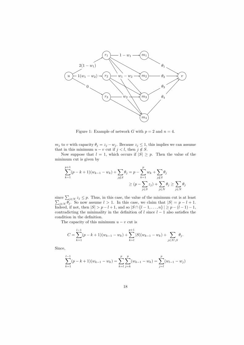
Let (z, w) ∈ H and consider a network G with node set given by V ={u, v, rk for k = 1, . . . , p + 1, mj for j ∈ N}. This network has arcs from u tork with capacity (p−k+1)(wk−1−wk) for all k = 1, . . . , p+1, arcs from rk to mj

with capacity wk−1 −wk for all j = k, . . . , n and k = 1, . . . , p+1, and arcs frommj to v with capacity θj for all j ∈ N . An example of this network with n = 4and p = 2 is given in Figure 1. The labels on the arcs in this figure representthe capacities. For the arcs from nodes rk to nodes mj , the capacity dependsonly on the node rk, so only the first outgoing arc from each rk is labeled. It iseasy to check that if this network has a flow from u to v of value

∑

j∈N θj , thenthe system (42) - (44) has a feasible solution. We will show that (z, w) ∈ Himplies the minimum u − v cut in the network is at least

∑

j∈N θj , and by themax-flow min-cut theorem, this guarantees a flow of this value exists, provingthat (z, w) ∈ conv(HI).

Now, consider a minimum u− v cut in the network G, defined by a node setU ⊂ V with u ∈ U and v /∈ U . Let S = {mj : j ∈ N \ U}. Note that if rk /∈ Uwe obtain an arc in the cut, from u to rk, with capacity (p− k +1)(wk−1 −wk),whereas if rk ∈ U , we obtain a set of arcs in the cut, from rk to mj for j ∈ Ssuch that j ≥ k, with total capacity

∑

j∈S∩{k,...,n}

(wk−1 − wk) = |S ∩ {k, . . . , n} |(wk−1 − wk).

Thus, because wk−1 ≥ wk we can assume that in this minimum u − v cutrk ∈ U if and only if |S ∩ {k, . . . , n} | < p− k + 1. Hence, if we let l = min{k =1, . . . , p+1 : |S∩{k, . . . , n} | ≥ p−k+1} then we can assume rk ∈ U for 1 ≤ k < land rk /∈ U for l ≤ k ≤ p + 1.

We now show that S ⊆ {l, . . . , n}. Indeed, suppose j < l. If j ∈ S then thecut includes arcs from rk to mj with capacity (wk−1 − wk) for all 1 ≤ k ≤ jyielding a total capacity of 1 − wj . If j /∈ S, then the cut includes an arc from

17

r1 m1

u r2 m2 v

r3 m3

m4

2(1 − w1)

1(w1 − w2)

0

1 − w1

w1 − w2

w2

θ1

θ2

θ3

θ4

Figure 1: Example of network G with p = 2 and n = 4.

mj to v with capacity θj = zj −wj . Because zj ≤ 1, this implies we can assumethat in this minimum u − v cut if j < l, then j /∈ S.

Now suppose that l = 1, which occurs if |S| ≥ p. Then the value of theminimum cut is given by

p+1∑

k=1

(p − k + 1)(wk−1 − wk) +∑

j /∈S

θj = p −

p∑

k=1

wk +∑

j /∈S

θj

≥ (p −∑

j∈S

zj) +∑

j∈N

θj ≥∑

j∈N

θj

since∑

j∈N zj ≤ p. Thus, in this case, the value of the minimum cut is at least∑

j∈N θj . So now assume l > 1. In this case, we claim that |S| = p − l + 1.Indeed, if not, then |S| > p− l + 1, and so |S ∩ {l − 1, . . . , n} | ≥ p− (l− 1)− 1,contradicting the minimality in the definition of l since l − 1 also satisfies thecondition in the definition.

The capacity of this minimum u − v cut is

C =

l−1∑

k=1

(p − k + 1)(wk−1 − wk) +

p+1∑

k=l

|S|(wk−1 − wk) +∑

j∈N\S

θj .

Since,

l−1∑

k=1

(p − k + 1)(wk−1 − wk) =

p∑

k=l

p∑

j=k

(wk−1 − wk) =

p∑

j=l

(wl−1 − wj)

18

it follows that

C = (p − l + 1)wl−1 −

p∑

k=l

wk + (1 − wl−1)|S| +∑

j∈N\S

θj

= (p − l + 1) −

p∑

k=l

wk +∑

j∈N\S

θj ≥∑

j∈N

θj

by (29) for k = l since S ⊆ {l, . . . , n} and |S| = p − l + 1.

We close this section by noting that inequalities (29) can be separated inpolynomial time. Indeed, suppose we wish to separate the point (z∗, w∗). Thenseparation can be accomplished by calculating

V ∗k = max

S∈Sk

∑

i∈S

z∗i +∑

i∈{k,...,p}\S

w∗i

= maxS∈Sk

{

∑

i∈S

θ∗i

}

+

p∑

i=k

w∗i

for k = 1, . . . , p where θ∗i = z∗i − w∗i for i = 1, . . . , p and θ∗i = z∗i for i =

p + 1, . . . , n. If V ∗k > p−k+1 for any k, then a violated inequality is found. Hence,

a trivial separation algorithm is to first sort the values θ∗i in non-increasingorder, then for each k, find the maximizing set S ∈ Sk by searching this list.This yields an algorithm with complexity O(n log n + p2) = O(n2). However,the complexity can be improved to O(n log n) as follows. Start by storing thep largest values of θ∗i over i ∈ {p + 1, . . . , n} in a heap, and define V ∗

p+1 = 0.Then, for k = p, . . . , 1 do the following. First insert θ∗k into this heap. Nextremove the largest value, say θ∗max, from the heap and finally calculate V ∗

k by

V ∗k = V ∗

k+1 + max {θ∗max, 0} + w∗k.

The initial heap construction is accomplished with complexity O(n log n), andthe algorithm then proceeds through p steps, each requiring insertion into aheap and removal of the maximum value from a heap, which can each be donewith O(log p) complexity, yielding overall complexity of O(n log n). For generalprobabilities πi, (heuristic) separation of inequalities (28) can be accomplishedby (heuristically) solving p knapsack problems.

5 Computational Experience

We performed computational tests on a probabilistic version of the classicaltransportation problem. We have a set of suppliers I and a set of customersD with |D| = m. The suppliers have limited capacity Mi for i ∈ I. There isa transportation cost cij for shipping a unit of product from supplier i ∈ I tocustomer j ∈ D. The customer demands are random and are represented bya random vector d ∈ R

m+ . We assume we must choose the shipment quantities

before the customer demands are known. We enforce the probabilistic constraint

P{∑

i∈I

xij ≥ dj , j = 1, . . . , m} ≥ 1 − ǫ (45)

19

where xij ≥ 0 is the amount shipped from supplier i ∈ I to customer j ∈ D.The objective is to minimize distribution costs subject to (45), and the supplycapacity constraints

∑

j∈D

xij ≤ Mi, ∀i ∈ I.

We randomly generated instances with the number of suppliers fixed at 40 andvarying numbers of customers and scenarios. The supply capacities and costcoefficients were generated using normal and uniform distributions respectively.For the random demands, we experimented with independent normal, dependentnormal and independent Poisson distributions. We found qualitatively similarresults in all cases, but the independent normal case yielded the most challenginginstances, so for our experiments we focus on this case. For each instance,we first randomly generated the mean and variance of each customer demand.We then generated the number n of scenarios required, independently acrossscenarios and across customer locations, as Monte Carlo samples with these fixedparameters. In most instances we assumed all scenarios occur with probability1/n, but we also did some tests in which the scenarios have general probabilities,which were randomly generated. CPLEX 9.0 was used as the MIP solver andall experiments were done on a computer with two 2.4 Ghz processors (althoughno parallelism is used) and 2.0 Gb of memory. We set a time limit of one hour.For each problem size we generated 5 random instances and, unless otherwisespecified, the computational results reported are averages over the 5 instances.

5.1 Comparison of Formulations

In Table 1 we compare the results obtained by solving our instances using

1. formulation PMIP given by (3) - (5),

2. formulation PMIP with strengthened star inequalities (11), and

3. the extended formulation of Sect. 4, but without (28) or (29).

When the strengthened star inequalities are not used, we still used the im-proved formulation of G corresponding to (10). Recall that the strengthenedstar inequalities subsume the rows defining the formulation PMIP; therefore,when using these inequalities we initially added only a small subset of the mpinequalities in the formulation. Subsequently separating the strengthened starinequalities as needed guarantees the formulation remains valid. For formulationPMIP without strengthened star inequalities, we report the average optimalitygap that remained after the hour time limit was reached, where we define theoptimality gap as the difference between the final upper and lower bounds, di-vided by the upper bound. For the other two formulations, which we refer toas the strong formulations, we report the geometric average of the time to solvethe instances to optimality. We used ǫ = 0.05 and ǫ = 0.1, reflecting the naturalassumption that we want to meet demand with high probability.

20

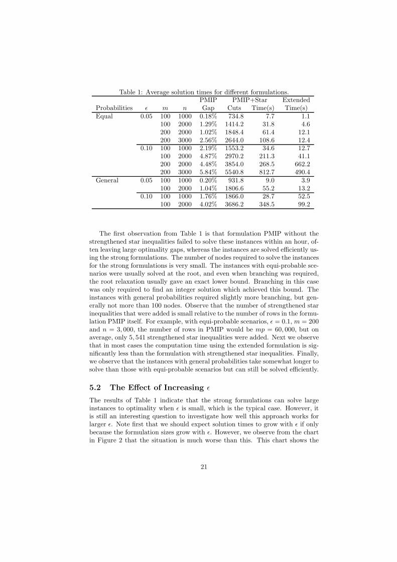
Table 1: Average solution times for different formulations.PMIP PMIP+Star Extended

Probabilities ǫ m n Gap Cuts Time(s) Time(s)Equal 0.05 100 1000 0.18% 734.8 7.7 1.1

100 2000 1.29% 1414.2 31.8 4.6200 2000 1.02% 1848.4 61.4 12.1200 3000 2.56% 2644.0 108.6 12.4

0.10 100 1000 2.19% 1553.2 34.6 12.7100 2000 4.87% 2970.2 211.3 41.1200 2000 4.48% 3854.0 268.5 662.2200 3000 5.84% 5540.8 812.7 490.4

General 0.05 100 1000 0.20% 931.8 9.0 3.9100 2000 1.04% 1806.6 55.2 13.2

0.10 100 1000 1.76% 1866.0 28.7 52.5100 2000 4.02% 3686.2 348.5 99.2

The first observation from Table 1 is that formulation PMIP without thestrengthened star inequalities failed to solve these instances within an hour, of-ten leaving large optimality gaps, whereas the instances are solved efficiently us-ing the strong formulations. The number of nodes required to solve the instancesfor the strong formulations is very small. The instances with equi-probable sce-narios were usually solved at the root, and even when branching was required,the root relaxation usually gave an exact lower bound. Branching in this casewas only required to find an integer solution which achieved this bound. Theinstances with general probabilities required slightly more branching, but gen-erally not more than 100 nodes. Observe that the number of strengthened starinequalities that were added is small relative to the number of rows in the formu-lation PMIP itself. For example, with equi-probable scenarios, ǫ = 0.1, m = 200and n = 3, 000, the number of rows in PMIP would be mp = 60, 000, but onaverage, only 5, 541 strengthened star inequalities were added. Next we observethat in most cases the computation time using the extended formulation is sig-nificantly less than the formulation with strengthened star inequalities. Finally,we observe that the instances with general probabilities take somewhat longer tosolve than those with equi-probable scenarios but can still be solved efficiently.

5.2 The Effect of Increasing ǫ

The results of Table 1 indicate that the strong formulations can solve largeinstances to optimality when ǫ is small, which is the typical case. However, itis still an interesting question to investigate how well this approach works forlarger ǫ. Note first that we should expect solution times to grow with ǫ if onlybecause the formulation sizes grow with ǫ. However, we observe from the chartin Figure 2 that the situation is much worse than this. This chart shows the

21

root LP solve times and optimality gaps achieved after an hour of computationtime for an example instance with equi-probable scenarios, m = 50 rows andn = 1, 000 scenarios at increasing levels of ǫ, using the formulation PMIP withstrengthened star inequalities. Root LP solve time here refers to the time untilno further strengthened star inequalities could be separated. We see that thetime to solve the root linear programs does indeed grow with ǫ as expected,but the optimality gaps achieved after an hour of computation time deterioratedrastically with growing ǫ. This is explained by the increased time to solve thelinear programming relaxations combined with an apparent weakening of therelaxation bound as ǫ increases.

ǫ

Figure 2: The effect of increasing ǫ.

5.3 Testing Inequalities (29)

With small ǫ the root relaxation given by the extended formulation is extremelytight, so that adding the inequalities (29) is unlikely to have a positive impact oncomputation time. However, for larger ǫ, we have seen that formulation PMIP,augmented with the strengthened star inequalities, and hence also the extendedformulation, may have a substantial optimality gap. We therefore investigatedwhether using inequalities (29) in the extended formulation can improve solutiontime in this case. In Table 2 we present results comparing solution times andnode counts with and without inequalities (29) for instances with larger ǫ. Weperformed these tests on smaller instances since these instances are already hardfor these values of ǫ. We observe that adding inequalities (29) at the root candecrease the root optimality gap significantly. For the instances that could besolved in one hour, this leads to a significant reduction in the number of nodes

22

Table 2: Results with and without inequalities (29).Root Gap Nodes Time(s) or Gap

m ǫ n Ext +(29) Ext +(29) Ext +(29)25 0.3 250 1.18% 0.67% 276.9 69.0 121.2 93.9

0.3 500 1.51% 0.58% 455.0 165.8 750.6 641.30.35 250 2.19% 1.50% 1259.4 409.0 563.2 408.40.35 500 2.55% 1.61% 2297.6 968.8 0.22% 0.06%

50 0.3 500 2.32% 2.00% 991.8 238.6 1.37% 1.41%0.3 1000 2.32% 1.75% 28.3 8.5 1.98% 1.66%

0.35 500 4.10% 3.31% 650.4 92.9 3.03% 2.66%0.35 1000 4.01% 3.23% 22.7 6.2 3.58% 3.17%

explored, and a moderate reduction in solution time. For the instances whichwere not solved in one hour, the remaining optimality gap was usually, but notalways, lower when the inequalities (29) were used. These results indicate thatwhen ǫ is somewhat larger, inequalities (29) may be helpful on smaller instances.However, they also reinforce the difficulty of the instances with larger ǫ, sinceeven with these inequalities, only the smallest of these smaller instances couldbe solved to optimality within an hour.

6 Concluding Remarks

We have presented strong integer programming formulations for linear programswith probabilistic constraints in which the right-hand side is random with finitedistribution. In the process we made use of existing results on mixing sets, andhave introduced new results for the case in which the mixing set additionallyhas a knapsack restriction. Computational results indicate that these formula-tions are extremely effective on instances in which reasonably high reliabilityis enforced, which is the typical case. However, instances in which the desiredreliability level is lower remain difficult to solve, partly due to increased sizeof the formulations, but more significantly due to the weakening of the for-mulation bounds. Moreover, these instances remain difficult even when usingthe inequalities which characterize the single row relaxation convex hull. Thissuggests that relaxations which consider multiple rows simultaneously need tobe studied to yield valid inequalities which significantly improve the relaxationbounds for these instances.

Our future work in this area will focus on addressing the two assumptionswe made at the beginning of this paper. The finite distribution assumption canbe addressed by using the results about the statistical relationship between aproblem with probabilistic constraints and its Monte Carlo sample approxima-tion to establish methods for generating bounds on the optimal value of theoriginal problem. Computational studies will need to be performed to establishthe practicality of this approach. We expect that relaxing the assumption that

23

only the right-hand side is random will be more challenging. A natural firststep in this direction will be to extend results from the generalized mixing set[14, 21] to the case in which an additional knapsack constraint is present.

References

[1] Ahmed, S., Shapiro, A.: The sample average approximation method forstochastic programs with integer recourse (2002). Preprint available atwww.optimization-online.org

[2] Atamturk, A., Nemhauser, G.L., Savelsbergh, M.W.P.: The mixed vertexpacking problem. Math. Program. 89, 35–53 (2000)

[3] Atlason, J., Epelman, M.A., Henderson, S.G.: Call center staffing withsimulation and cutting plane methods. Ann. Oper. Res. 127, 333–358(2004)

[4] Beraldi, P., Ruszczynski, A.: A branch and bound method for stochasticinteger programs under probabilistic constraints. Optim. Methods Softw.17, 359–382 (2002)

[5] Cheon, M.S., Ahmed, S., Al-Khayyal, F.: A branch-reduce-cut algorithmfor the global optimization of probabilistically constrained linear programs.Math. Program. 108, 617–634 (2006)

[6] Dentcheva, D., Prekopa, A., Ruszczynski, A.: Concavity and efficientpoints of discrete distributions in probabilistic programming. Math. Pro-gram. 89, 55–77 (2000)

[7] Guan, Y., Ahmed, S., Nemhauser, G.L.: Sequential pairing of mixed integerinequalities. Discrete Optim. 4, 21–39 (2007)

[8] Gunluk, O., Pochet, Y.: Mixing mixed-integer inequalities. Math. Program.90, 429–457 (2001)

[9] Henrion, R., Li, P., Moller, A., Steinbach, M.C., Wendt, M., Wozny, G.:Stochastic optimization for operating chemical processes under uncertainty.In: M. Grotschel, S. Krunke, J. Rambau (eds.) Online Optimization ofLarge Scale Systems, pp. 457–478 (2001)

[10] Henrion, R., Moller, A.: Optimization of a continuous distillation processunder random inflow rate. Computers and Mathematics with Applications45, 247–262 (2003)

[11] Lejeune, M.A., Ruszczynski, A.: An efficient trajectory method for proba-bilistic inventory-production-distribution problems. Oper. Res. (Forthcom-ing, 2007)

24

[12] Luedtke, J.: Integer programming approaches to two non-convex optimiza-tion problems. Ph.D. thesis, Georgia Institute of Technology, Atlanta, GA(2007)

[13] Luedtke, J., Ahmed, S., Nemhauser, G.: An integer programming ap-proach for linear programs with probabilistic constraints. In: M. Fischetti,D. Williamson (eds.) IPCO 2007, Lect. Notes Comput. Sci., pp. 410–423.Springer-Verlag, Berlin (2007)

[14] Miller, A.J., Wolsey, L.A.: Tight formulations for some simple mixed inte-ger programs and convex objective integer programs. Math. Program. 98,73–88 (2003)

[15] Murr, M.R., Prekopa, A.: Solution of a product substitution problem usingstochastic programming. In: S.P. Uryasev (ed.) Probabilistic ConstrainedOptimization: Methodology and Applications, pp. 252–271. Kluwer Aca-demic Publishers (2000)

[16] Prekopa, A.: On probabilistic constrained programmming. In: H.W. Kuhn(ed.) Proceedings of the Princeton Symposium on Mathematical Program-ming, pp. 113–138. Princeton University Press, Princeton, N.J. (1970)

[17] Prekopa, A.: Probabilistic programming. In: A. Ruszczynski, A. Shapiro(eds.) Stochastic Programming, Handbooks in Operations Research and

Management Science, vol. 10, pp. 267–351. Elsevier (2003)

[18] Ruszczynski, A.: Probabilistic programming with discrete distributions andprecedence constrained knapsack polyhedra. Math. Program. 93, 195–215(2002)

[19] Shapiro, A., Homem-de-Mello, T.: On the rate of convergence of optimalsolutions of Monte Carlo approximations of stochastic programs. SIAMJ. Optim. 11, 70–86 (2000)

[20] Takyi, A.K., Lence, B.J.: Surface water quality management using amultiple-realization chance constraint method. Water Resources Research35, 1657–1670 (1999)

[21] Van Vyve, M.: The continuous mixing polyhedron. Math. Oper. Res. 30,441–452 (2005)

25