an integrated intelligent technique for monthly rainfall
TRANSCRIPT

An Integrated Intelligent Technique for Monthly Rainfall Time Series Prediction
Jesada Kajornrit, Kok Wai Wong, Chun Che Fung School of Engineering and Information Technology,
Murdoch University, Murdoch, Western Australia, 6150 [email protected], k.wong, [email protected]
Yew Soon Ong School of Computer Engineering,
Nanyang Technological University, Singapore, 639798 [email protected]
Abstract—This paper proposes a methodology to create an interpretable fuzzy model for monthly rainfall time series pre-diction. The proposed methodology incorporates the advantag-es of artificial neural network, fuzzy logic and genetic algo-rithm. In the first step, the differences between the time series data are calculated and they are used to define the interval between the membership functions of a Mamdani-type fuzzy inference system. Next, artificial neural network is used to develop the model from input-output data and the established model is then used to extract the fuzzy rules. The parameters of the created fuzzy model are then optimized by using genetic algorithm. The proposed model was applied to eight monthly rainfall time series data in the northeast region of Thailand. The experimental results showed that the proposed model pro-vided satisfactory prediction accuracy when compared to other commonly-used prediction models. Due to the interpretability nature of the model, human analysts can gain insight know-ledge of the data to be modeled.
Keywords—Time Series Prediction; Monthly Rainfall Data; Fuzzy Logic; Artificial Neural Network; Genetic Algorithm; Interpretability; Northeast Region of Thailand
I. INTRODUCTION In agricultural countries such as Thailand, efficient water
management is necessary to provide effective flood and drought prevention, reservoir operation, contract negotia-tion, and irrigation scheduling [1]. One of the key issues in water management is the accurate forecasting of rainfall. Accurate rainfall forecasting will provide accurate and time-ly projection of flow forecasting in the river basins. Howev-er, due to the complexity nature of the rainfall, this task is not trivial. Hydrological processes such as rainfall depend on many complex factors that are not clearly understood [2]. Therefore, to perform this task, data-driven based models seem to be a promising approach to tackle this problem.
Recently, intelligent techniques such as Artificial Neural Network (ANN) have been successfully adopted in hydro-logical studies [3]. These techniques have provided consi-derable accurate results and they could be established with-out the need of prior knowledge [4]. Consequently, such techniques are attractive for researchers and hydrologists. Examples are Somvanshi et al. [5] who applied ANN to rainfall time series data whereas Jain and Kumar [6] applied ANN to streamflow time series data. Their results demon-
strate that ANN had provided better accurate results over the conventional Box-Jenkins (BJ) approach.
Due to the high flexibility of ANN, modular concept can be applied to enhance the prediction accuracy. Wu et al. [4] proposed ANN and modular ANN with data preprocessing techniques to predict rainfall time series. They applied three preprocessing techniques to smoothen time series data. Fur-thermore, they also successfully applied ANN combined with support vector regression in their subsequent works [2]. However, although ANN is able to provide good quantita-tive results, the qualitative drawback of ANN still exits. The model interpretability is deprived due to the black-box na-ture of ANN model.
Interpretability is another important issue in data-driven modeling. Interpretable models can provide insight know-ledge of the data to be modeled when prior knowledge is unknown [7]. Fuzzy Logic (FL) [8] is a grey-box model which has been successful applied in many disciplines in-cluding hydrological areas [9], [10]. Compared to the black-box nature of ANN, fuzzy modeling formulates the system knowledge with rules in a transparent way for interpretation and analysis. However, establishing an efficient interpreta-ble fuzzy system is not an easy task because interpretability and accuracy issues can be contrasting objectives [11].
Adaptive Neuro Fuzzy Inference System (ANFIS) [12] is another technique that has been successfully applied in hy-drological area. ANFIS is a Sugeno-type FIS [13] which has its parameters adjusted to the training data by using back-propagation algorithm. Nayak et al. [14] and Kermani et al. [15] introduced ANFIS model to river flow time series pre-diction. Wang et al. [16] showed the performance of ANFIS in predicting monthly discharge time series. Although AN-FIS is more transparent to human analysts than ANN, its consequent part is still not intuitive as much as Mamdani-type FIS [17]. Furthermore, applications of ANFIS in hy-drology usually belong to the class of prototype-based mod-eling. This technique sometimes causes the model to loss its interpretability during the learning process [7].
As mentioned, this paper proposes a methodology to create an interpretable Mamdani-type FIS model to monthly rainfall time series prediction problem. The proposed me-thodology combined advantages of ANN, FL and Genetic Algorithm (GA) [18] and applied to eight monthly rainfall
2014 IEEE International Conference on Fuzzy Systems (FUZZ-IEEE) July 6-11, 2014, Beijing, China
978-1-4799-2072-3/14/$31.00 ©2014 IEEE 1632
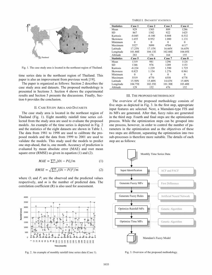
Fig. 1. The case study area is located in the northeast region of Thailand.
time series data in the northeast region of Thailand. This paper is also an improvement from previous work [19].
The paper is organized as follows: Section 2 describes the case study area and datasets. The proposed methodology is presented in Sections 3. Section 4 shows the experimental results and Section 5 presents the discussions. Finally, Sec-tion 6 provides the conclusion.
II. CASE STUDY AREA AND DATASETS The case study area is located in the northeast region of
Thailand (Fig. 1). Eight monthly rainfall time series col-lected from the study area are used to evaluate the proposed models. An example of the time series is depicted in Fig. 2 and the statistics of the eight datasets are shown in Table 1. The data from 1981 to 1998 are used to calibrate the pro-posed models and the data from 1999 to 2001 are used to validate the models. This study used the models to predict one step-ahead, that is, one month. Accuracy of prediction is evaluated by mean absolute error (MAE) and root mean square error (RMSE) as given in equation (1) and (2). ∑ | |⁄ (1) ∑ ⁄ (2) where Oi and Pi are the observed and the predicted values respectively, and m is the number of predicted data. The correlation coefficient (R) is also used for assessment.
Fig. 2. An example of monthly rainfall time series data (Case 1).
TABLE I. DATASETS’ STATISTICS
Statistics Case 1 Case 2 Case 3 Case 4 Mean 929 1303 889 1286 SD 867 1382 922 1425 Kurtosis -0.045 -0.100 0.808 0.532 Skewness 1.655 0.952 1.080 1.131 Minimum 0 0 0 0 Maximum 3527 5099 4704 6117 Latitude 17.25N 17.15N 16.66N 16.65N Longitude 101.80E 104.13E 102.88E 104.05E Altitude 283 176 164 155 Statistics Case 5 Case 6 Case 7 Case 8 Mean 1319 981 1296 1124 SD 1346 976 1289 1153 Kurtosis -0.224 1.229 1.590 1.725 Skewness 0.825 1.154 1.276 0.961 Minimum 0 0 0 0 Maximum 5519 4770 6558 6778 Latitude 15.50N 15.40N 14.63N 15.40N Longitude 104.75E 102.35E 101.30E 103.40E Altitude 129 152 476 152
III. THE PROPOSED METHODOLOGY The overview of the proposed methodology consists of
five steps as depicted in Fig. 3. In the first step, appropriate input features are selected. Next, a Mamdani-type FIS and its MFs are generated. After that, fuzzy rules are generated in the third step. Fourth and final steps are the optimization process. While the optimization steps can be grouped into one process, however, in order to control the number of pa-rameters in the optimization and as the objectives of these two steps are different, separating the optimization into two sub-processes is therefore more suitable. The details of each step are as follows:
Fig. 3. Overview of the proposed methodology.
0
500
1000
1500
2000
2500
3000
3500
4000
1 12 23 34 45 56 67 78 89 100
111
122
133
144
155
166
177
188
199
210
221
232
243
Rain
fall
(mm
)
Time (month)
Input Identification
Generate Fuzzy MFs
Generate Fuzzy Rules
Optimize Rainfall MFs
Optimize Time MFs
Monthly Time Series Data
Mamdani's Fuzzy Model
First Difference
Artificial Neural Network
Genetic Algorithm
Genetic Algorithm
ACF and PACF
Thailand
1 2
3 4
5 6
7 8
N
1633

A. Input identification
The objective of predicting rainfall using antecedent val-ues is to generalize a relationship in the following form:
(3)
where is a m-dimensional input vector representing rain-fall value with different time lags and y is a one-dimensional output representing predicted rainfall value. In general, is not known prior and there is no consistent theory to define
for non-linear techniques [16]. In general, two statistical methods, the autocorrelation
function (ACF) and the partial autocorrelation function (PACF), are employed to determine the dimension m of input vectors [2], [16]. The ACF and PACF are generally used in diagnosing the order of the autoregressive process. Fig. 4 shows an example of ACF and PACF of the dataset. ACF exhibits the peak value at lag 12 and PACF showed a signifi-cant correlation at 95% confidence level interval up to lag 12. Therefore, these suggested that twelve antecedent rainfall values contain sufficient information to predict future rain-fall.
However, for a FIS model, selecting 12 lags can result in the increase of complexity in fuzzy rules and will cause the readability problem, especially, in the antecedent part [7]. Furthermore, due to the issue of curse of dimensionality, the number of fuzzy parameters could increase tremendously. Even using the phase space reconstruction to identify input may not be a good solution to this problem. However, as the monthly time series is periodic in nature, adding time coeffi-cient as a supplementary feature is a promising approach [20], [21], [22].
Time coefficient (Ct) is used to assist the model to scope prediction into specific period. It may be Ct = 2 (wet and dry period) or Ct = 12 (calendar months). This study adopted Ct = 12 as a supplementary feature. Once Ct is added into the system, 12-lag information may be redundant. This study proposed the use of first lag that crosses the confidence in-terval line as the minimum information for the model. There-fore, two first lags of rainfalls and Ct are considered as the model inputs. This selection conforms to the suggestion in [21] and [22] in that 2-lag antecedence is sufficient informa-tion for monthly time series prediction.
B. Generate Fuzzy MFs In order to create MFs for an interpretable fuzzy system,
two aspects must be considered simultaneously. The created MFs should be distinguish [7], [23] and should reflect the nature of the time series at the same time. Huarng [24] sug-gested that the appropriate interval length between two con-secutive MFs for time series data should be at least a half of the fluctuations in the time series. The fluctuation in time series data is the absolute value of the first difference of any two consecutive data. This concept is adopted in this study and it is adapted to fit to the nature of the monthly rainfall data.
In this paper, the absolute values of the first difference of time series is calculated and percentile at 25, 50 and 75 of these values are adopted to explain the fluctuation of the
rainfall at low, medium and high periods. The low period of the rainfall is defined as zero to percentile 50 of the rainfall values, the medium period is defined as percentile 50 to percentile 75. Above percentile 75 are defined as high pe-riod. This procedure is applied to first lag, second lag inputs and output of the fuzzy model. In this study, triangle MF is preferred to Gaussian MF because the asymmetric characte-ristic of the MF is more flexible.
Fig. 4. ACF and PACF of rainfall time series data (Case 1).
An example of the generated MFs is shown in Fig. 5. It is clear that these generated MFs show the completeness of partition of input variable [7], [23] and the normalization [7], [23] criteria for the interpretable fuzzy system.
Fig. 5. An example of Ct's MFs and Rainfall's MFs (Case 1).
0 10 20 30 40 50 60-0.5
0
0.5
1
Lag
Sam
ple
Aut
ocor
rela
tion
Sample Autocorrelation Function (ACF)
0 10 20 30 40 50 60-0.4
-0.2
0
0.2
0.4
0.6
0.8
1
Lag
Sam
ple
Par
tial A
utoc
orre
latio
ns
Sample Partial Autocorrelation Function
0 0.1 0.2 0.3 0.4 0.5 0.6 0.7 0.8 0.9 1
0
0.2
0.4
0.6
0.8
1
month
Deg
ree
of
me
mb
ersh
ip
jan feb mar apr may jun jul agu sep oct nov dec
0 0.2 0.4 0.6 0.8 1 1.2
0
0.2
0.4
0.6
0.8
1
Rainfall
Deg
ree
of
me
mb
ersh
ip
A1 A2 A3 A4 A5 A6 A7 A8 A9
95% Confidence Interval Line
95% Confidence Interval Line
1634

C. Generate Fuzzy Rules One drawback of FL is its lack of self-learning ability to
generalize the input-output relationships from training data. This study uses the learning ability from ANN to create fuzzy rules. The procedure to create fuzzy rules is as fol-lows:
Step 1. Use one hidden layer back-propagation neural net-work (BPNN) to learn from the training data. The number of input nodes is 3 and output node is 1. The number of hidden node is selected by trial and error.
Step 2. Prepare the set of input data. The set of input data is all the points in the input space where the degree of mem-bership values is 1 in all dimensions. (This input data are the antecedent part of the fuzzy rules).
Step 3. Feed the input data into the BPNN, the output of BPNN are then mapped to the nearest MF in the output di-mension of fuzzy model. (This output data are the conse-quence part of the fuzzy rules).
Using this procedure, the readability fuzzy rules are gener-ated in the form: "IF month = M AND first lag = A AND second lag = B THEN rainfall = C".
D. Optimize Fuzzy MFs
In Fig. 3, the process consists of rainfall's MFs and time's MFs optimization. The first one is to optimize MFs of input 2, input 3 and output, while the second one is to optimize input 1's MFs. Actually, such processes could be done in a single process. However, the objectives of these two processes are different and to control the number of parame-ters in each optimization process, this study separates the optimization process into two sub-processes.
The objective of the first one is to fit the fuzzy rules and fuzzy MFs of rainfall variable. As these two parameters come from two approaches, they may not fit well. The ob-jective of the second optimization is to capture uncertainty in time dimension. This study hypothesizes that the substan-tial uncertainty in time dimension will be well extracted when rainfall parameters are already fitted.
In the first part of optimization process, the GA chromo-some consists of the sequence of input 2, input 3 and output respectively. In turn, the inputs and output are the sequence of MFs which consists of three parameters of triangle MF (a, b, c). The parameters are allowed to be searched in a small space [25], [26].
Let a, b and c be the initial value of MF's parameters and let x be a parameter to be optimized, the search space of x is [x - α, x + α] and α is defined as
(4)
where σ is user's parameter ranged in [0,1]. In other word, searching space α is depended on the size of the initial MF.
In the second part of the optimization process, the GA chromosome is the sequence of MFs of input 1. The search space is set in a different way.
Fig. 6. Search space of MFs in time input dimension.
Fig. 6 demonstrates a conceptual example of how to set the search space of parameter a, b and c. Search space of a and c are set in this manner in order to allow the FIS to cap-ture the uncertainty in time between months and search space of b is set in this manner in order to allow FIS to re-duce some firing strength of that month. Furthermore, this setting is to prevent the FIS model from indistinguishability [7]. The search space for parameters a and c are equal to the intersection range of the two MFs and half of the intersec-tion for parameter b as demonstrated by the arrows in Fig. 6.
For both processes, the fitness function is the minimize sum square error between observed values (O) and predicted values (P) of the training data and it is given as ∑ (5)
where S is the number of training data.
IV. EXPERIMENTAL RESULTS
In order to assess the prediction accuracy, the proposed model is compared to some hydrological commonly-used models, namely, Autoregressive Moving Average (ARMA) [4], [16], BPNN [2], [4], [5], [6] and ANFIS [14], [15], [16]. Furthermore, the proposed model is also compared to BPNN that used to create fuzzy rules and the model before opti-mized. A. Models preparation
In order to select the optimal ARMA models, Akaike In-formation Criterion (AIC) is adopted [4], [16]. This study generated ARMA models from calibration data by replacing parameters p and q of ARMA model from 0 to 12. The pa-rameters that gave lowest AIC value were used for ARMA model. Table 2 shows the ARMA models for eight datasets.
TABLE II. THE SELECTED PARAMETERS AND AIC VALUES
Case (p,q) AIC Case (p,q) AIC 1 (4,4) 13.417 5 (5,3) 13.751 2 (10,9) 13.982 6 (12,1) 13.536 3 (6,3) 13.379 7 (12,0) 14.334 4 (8,11) 14.182 8 (11,2) 13.850
For BPNN and ANFIS, there is no consistent theory to se-
lect the number of input. However, the work of [2], [4], [16] recommended the use of ACF and PACF to investigate the appropriate inputs. Considering ACF and PACF in Fig. 4, it pointed out that time series show autoregressive process up
May Jun Jul Aug Apr
la ua lc uc
lb ub
1635

to lag 12. Therefore, 12-lag inputs should provide sufficient information for the models.
TABLE III. THE ARCHITECTURE AND EPOCH OF BPNNS AND ANFIS
Case hn / cls Case hn / cls 1 3 / 2 5 2 / 2 2 2 / 2 6 3 / 3 3 3 / 3 7 2 / 2 4 3 / 2 8 3 / 2
The architecture of BPNN and ANFIS are twelve input
nodes and one output node. The optimal number of parame-ters was selected by trial and error. To investigate the op-timal number of parameters, calibration data were separated into two parts. The first part was used to train models and the second part was used to test the models.
In the case of BPNN, the experiments varied the number of hidden nodes from 2 to 6. An example of the results is shown in Fig. 7 (top). From the experiment, the number of two or three hidden nodes can provide minimum error. Ta-ble 3 summarizes the number of hidden node (hn) of BPNN of eight datasets. Furthermore, when the number of training epochs is larger than 15, the error of testing data started to increase. Therefore, the number of epoch was limited to 15.
In the case of ANFIS, the prototype-based model is used. Sugeno-type FIS was generated from fuzzy c-mean cluster-ing technique and was then optimized by ANFIS procedure. An example of the results is shown in Fig 7 (bottom). The experiment pointed out that small number of cluster pro-vided better prediction. The effect of error to number of epochs is more sensitive than BPNN. Only 2 or 3 epochs are enough to generalize data. The number of selected cluster (cls) of ANFIS is presented in Table 3.
In the case of the proposed model, BPNN used to create fuzzy rules were selected in the same manner. The value of σ in the first optimization was set to 0.25 so as to preserve the shape of MFs after optimized. The number of population was 100 for both optimizations and the number of genera-tion was 30 and 15 for first and second optimization respec-tively, where the best and average fitness values were met. Reproduction scheme elite count was set to 2 and crossover fraction was set to 0.8.
B. Quantitative results
From now on, BPNN12 refers to BPNN with twelve ante-cedence lags input, BPNN3 refers to BPNN with Ct and two antecedence lags input, MFIS-ORG is the proposed model before optimization, MFIS-OPT1 and MFIS-OPT2 are the proposed models after the first and the second optimization respectively. Table 4, 5 and 6 show the experimental results. MAE and RMSE of each case are normalized by its mean of the dataset. The Average column in the Tables 4 and 5 show the average values of these normalized errors.
According to these average values, the accuracy of all models are ranked as MFIS-OPT2 > MFIS-OPT1 > BPNN3 > MFIS-ORG > ANFIS > ARMA > BPNN12. In comparison with the commonly-used models in hydrology, the proposed models can meet the accuracy requirement. These results also point out that:
• BPNN12 did not show superior results than ARMA in this study. However, it does not mean that BPNN12 is not an efficient method. The dataset in this study are relatively small in comparison with the datasets used in other studies mentioned before. The number of training data may not be enough when BPNN's input is large (12 dimensions). In general, efficient ANN models prefer large training data. The accuracy of BPNN12 may be better if more training data are available.
• ANFIS is capable to capture the uncertainty in the data because it provided better results than BPNN12 and AR-MA. However, the use of ANFIS should be handled with care because such model showed higher sensitivity than BPNN12. As can be seen in Fig. 7, ANFIS tended to loss generalization in only few epochs. This is one reason that BPNN was used instead of ANFIS to generate fuzzy rules in the proposed method.
• Using Ct as the supplementary feature for periodic time series data is an efficient way to improve the prediction accuracy. According to the experimental results, BPNN3 provided considerable improvement from BPNN12 and ANFIS.
• Conversion from BPNN3 to MFIS-ORG inevitably de-creases some prediction accuracy. However, this issue can be address by the optimization process. One can see that the prediction accuracy of MFIS-ORG was improved when fuzzy rules and MFs were fitted well (MFIS-OPT1).
• The uncertainty in the time dimension has significant ef-fect to the prediction accuracy of the proposed models. Once the MFs in time dimension were optimized (MFIS-OPT2), the accuracy of the proposed models were im-proved.
Fig 7. Trial & error process of (top) BPNN and (bottom) ANFIS.
0.130
0.140
0.150
0.160
0.170
0.180
0.190
5 10 15 20 25 30 35 40 45 50
Nor
mal
ized
MA
E
Epochs
2 3 4 5 6
0.07000.0800
0.0900
0.10000.1100
0.1200
0.1300
0.14000.1500
1 2 3 4 5 6 7 8 9 10
Nor
mal
ized
MA
E
Epochs
2 3 4 5
1636

TABLE IV. MEAN ABSOLUTE ERROR (MAE) OF VALIDATION PERIOD Model Case 1 Case 2 Case 3 Case 4 Case 5 Case 6 Case 7 Case 8 Average
ARMA 688 626 529 707 823 560 671 471 0.562 BPNN12 526 631 551 793 806 648 736 592 0.581 ANFIS 516 505 515 671 683 585 661 473 0.511
BPNN3 476 512 443 631 722 518 639 486 0.487 MFIF-ORG 493 508 472 681 679 530 581 547 0.496 MFIS-OPT1 452 503 444 614 662 515 574 491 0.469 MFIS-OPT2 449 497 373 608 613 506 571 461 0.448
TABLE V. ROOT MEAN SQUARE ERROR (RMSE) OF VALIDATION PERIOD Model Case 1 Case 2 Case 3 Case 4 Case 5 Case 6 Case 7 Case 8 Average
ARMA 888 883 771 1028 1162 836 844 645 0.782 BPNN12 719 926 866 1243 1153 994 963 852 0.851 ANFIS 715 773 752 982 1017 829 864 679 0.732
BPNN3 710 827 701 979 1085 752 818 701 0.724 MFIS-ORG 725 848 714 1018 1020 781 760 791 0.735 MFIS-OPT1 679 814 690 952 992 750 757 711 0.700 MFIS-OPT2 678 802 597 911 934 741 746 672 0.670
TABLE VI. CORRELATION COEFFICIENT (R) OF VALIDATION PERIOD Model Case 1 Case 2 Case 3 Case 4 Case 5 Case 6 Case 7 Case 8 Average
ARMA 0.539 0.787 0.543 0.797 0.666 0.587 0.466 0.776 0.645 BPNN12 0.731 0.761 0.572 0.740 0.656 0.465 0.371 0.664 0.620 ANFIS 0.764 0.844 0.583 0.835 0.738 0.613 0.468 0.772 0.702
BPNN3 0.749 0.822 0.632 0.846 0.703 0.695 0.570 0.757 0.722 MFIS-ORG 0.748 0.824 0.623 0.809 0.741 0.663 0.612 0.691 0.714 MFIS-OPT1 0.794 0.838 0.645 0.837 0.755 0.704 0.630 0.750 0.744 MFIS-OPT2 0.800 0.844 0.732 0.855 0.781 0.718 0.634 0.767 0.766
In summary, the details of conversion from BPNN3 to MFIS-OPT2, the results showed that not all cases provided significant improvement. Case 3, 5 and 7 provided large improvement up to 10 percent. Case 1, 4 and 8 provided moderate improvement about 5 percent. Case 2 and 6 showed small improvement approximate 2 percent. This difference is subject to
• If the uncertainty in time series data is not strong, the pre-diction accuracy between those two models may not be different because BPNN is capable of handling weak un-certainty.
• In order to preserve the interpretability of the proposed model, search space is limit into a small region. GA may not be able to find better optimal solution in the constraint search space.
C. Qualitative results
Fig. 8 shows an example of fuzzy parameters of MFIS-OPT2. As the model's parameters are transparently presented in term of fuzzy rules and fuzzy MFs, human analysts can make use of his/her knowledge to enhance the model capa-bility [9]. Furthermore, when the prior knowledge of the data to be modeled is unclear or unknown, these fuzzy pa-
rameters can provide information to better understand the data.
In the work of [7], interpretability of fuzzy systems is di-vided into fuzzy set level and fuzzy rule level. Fuzzy set levels is low-level interpretability and fuzzy rule level is high-level interpretability. It will be used herein.
In the fuzzy set level, one can see that the distinguisha-bility, normality and completeness of partition in input space of MFs were preserved after optimization. Optimized MFs are rather well structured and clear. These are impor-tant criteria in the fuzzy interpretability issues because these criteria are generally lost during the optimization process.
The number of fuzzy sets in each input dimension ranges from 9 - 13 depending on the fluctuation in time series. Al-though these numbers are higher than those proposed by [7] (an appropriate number of MFs in each input should not exceed 7 ± 2), these numbers are necessary because they are good explanation to the fluctuation in the time series data.
In the fuzzy rule level, the proposed model provides good readability of single rules with only three conditions in an-tecedent part while ANFIS has twelve conditions. Since the fuzzy rules are extracted from generalized BPNN3 by using mapping procedure, the consistence and completeness of fuzzy rules is met. In case of the transparency of the rules structure, as the proposed model presents the month feature
1637

Fig. 8. An example of fuzzy parameters in MFIS-OPT2 (Case 1)
as an input to the system, the fuzzy rule, IF month=M AND 1stlag=A AND 2ndlag=B THEN rainfall= C, can character-ize or explain the monthly rainfall time series data in a hu-man understanding manner.
However, although many interpretable fuzzy criteria have been met, a modulate number of fuzzy rules is still the prob-lem because the proposed model has a large numbers of fuzzy rules. For example, if the number of MFs in the model is 9, the number of fuzzy rules generated is 972. This prob-lem may need to be addressed.
For the monthly rainfall time series data in this study, a number of redundant rules (i.e., high rainfall in dry period and vice versa) can be removed later by human analysts. This can be done by using expert knowledge or by observ-ing from historical records. Thank to the good readability structure of the fuzzy rules, this removal is not a compli-cated task.
V. DISCUSSIONS Up to this point, the experimental results have been pre-
sented in term of quantitative and qualitative aspects. The results showed that the proposed model provided satisfacto-ry prediction accuracy and acceptable model interpretability. However, the main objective of the proposed model is to create an efficient method to gain insight into the monthly rainfall time series data.
Fig. 9 presents the uncertainty in time dimension of monthly rainfall time series data via fuzzy parameters. These fuzzy MFs allow human analysts to investigate the uncertainty of the rainfall data between months. Conse-quently, further analysis in the data could be enhanced.
Fig. 9. A presentation of uncertainty in time dimension through fuzzy MFs
(Case 1 to Case 8 are presented from top to bottom)
0 0.1 0.2 0.3 0.4 0.5 0.6 0.7 0.8 0.9 1
0
0.5
1
month
Deg
ree
of
mem
bers
hip jan f eb mar apr may jun jul agu sep oct nov dec
0 0.2 0.4 0.6 0.8 1 1.2
0
0.5
1
lag1
Deg
ree
of m
emb
ersh
ip
A1 A2 A3 A4 A5 A6 A7 A8 A9
0 0.2 0.4 0.6 0.8 1 1.2
0
0.5
1
lag2
Deg
ree
of m
emb
ersh
ip
B1 B2 B3 B4 B5 B6 B7 B8 B9
0 0.2 0.4 0.6 0.8 1 1.2
0
0.5
1
rainfall
Deg
ree
of m
emb
ersh
ip
C1 C2 C3 C4 C5 C6 C7 C8 C9
0 0.1 0.2 0.3 0.4 0.5 0.6 0.7 0.8 0.9 1
0
0.5
1
month
Deg
ree
of
mem
bers
hip jan f eb mar apr may jun jul agu sep oct nov dec
0 0.1 0.2 0.3 0.4 0.5 0.6 0.7 0.8 0.9 1
0
0.5
1
month
Deg
ree
of
mem
bers
hip jan f eb mar apr may jun jul agu sep oct nov dec
0 0.1 0.2 0.3 0.4 0.5 0.6 0.7 0.8 0.9 1
0
0.5
1
month
Deg
ree
of
mem
bers
hip jan f eb mar apr may jun jul agu sep oct nov dec
0 0.1 0.2 0.3 0.4 0.5 0.6 0.7 0.8 0.9 1
0
0.5
1
month
Deg
ree
of m
embe
rshi
p jan f eb mar apr may jun jul agu sep oct nov dec
0 0.1 0.2 0.3 0.4 0.5 0.6 0.7 0.8 0.9 1
0
0.5
1
month
Deg
ree
of m
embe
rshi
p jan f eb mar apr may jun jul agu sep oct nov dec
0 0.1 0.2 0.3 0.4 0.5 0.6 0.7 0.8 0.9 1
0
0.5
1
month
Deg
ree
of m
emb
ersh
ip
jan f eb mar apr may jun jul agu sep oct nov dec
0 0.1 0.2 0.3 0.4 0.5 0.6 0.7 0.8 0.9 1
0
0.5
1
month
Deg
ree
of m
embe
rshi
p jan f eb mar apr may jun jul agu sep oct nov dec
0 0.1 0.2 0.3 0.4 0.5 0.6 0.7 0.8 0.9 1
0
0.5
1
month
Deg
ree
of m
embe
rshi
p jan f eb mar apr may jun jul agu sep oct nov dec
0 0.1 0.2 0.3 0.4 0.5 0.6 0.7 0.8 0.9 1
0
0.5
1
month
Deg
ree
of m
emb
ersh
ip
jan f eb mar apr may jun jul agu sep oct nov dec
1638

To analyze this uncertainty, the method such as prototype-based fuzzy modeling may not be appropriate for this task. The original shape of month's MFs can be loss when the prototypes are created or during the optimization process. Consequently, the interpretability will be inevitably de-creased.
In this methodology, the fuzzy MFs have firstly been created based on the characteristics of time series data. Thus, the requirement is how to create the fuzzy rules for the model. Among several neuro-fuzzy methods [9], coop-erative neuro fuzzy technique [19] seems to be the most appropriate.
This cooperative neuro-fuzzy technique uses BPNN to generalize the input-output relationships from training data and the BPNN is then used to extract fuzzy rules. This tech-nique is matched to the requirement of methodology, in which the original shape of MFs can be preserved when the fuzzy rules are created.
VI. CONCLUSION Accurate rainfall forecasting is crucial for reservoir opera-
tion, flood and drought prevention and contract negotiation because it can provide accurate and timely future projection of the flow forecasting. This study proposed an integration of intelligent techniques, namely, fuzzy logic, artificial neural network and genetic algorithm to create an interpret-able fuzzy model for monthly rainfall time series prediction. Eight monthly rainfall time series data in the northeast re-gion of Thailand were used to evaluate the proposed model. The experimental results showed that the proposed model provided satisfactory prediction accuracy when it was com-pared to conventional methods. Furthermore, the proposed model is transparent to human analysts through fuzzy para-meters. The advantage of the proposed model is that it pro-vides the overview of uncertainty in time dimension be-tween months in form of fuzzy MFs. This is an important issue for human analysts to gain insight in the data to be modeled when a prior knowledge is unclear or unknown.
REFERENCES [1] S. Araghinejad, M. Azmi, and M. Kholghi, “Application of artificial
neural network ensembles in probabilistic hydrological forecasting,” Journal of Hydrology, vol. 407, pp. 94-104, 2011.
[2] C.L. Wu and K.W. Chau, “Prediction of rainfall time series using modular soft computing methods,” Engineering applications of artifi-cial intelligence, vol. 26, pp. 997-1007, 2013.
[3] ASCE task committee on application of artificial neural networks in hydrology, “Artificial neural networks in hydrology. II: Hydrologic applications,” Journal of hydrologic engineering, vol. 5(2), pp. 124–137, 2000.
[4] C.L. Wu, K.W. Chau, and C. Fan, “Prediction of rainfall time series using modular artificial neural networks coupled with data-preprocessing techniques,” Journal of Hydrology, vol. 389, pp. 146-167, 2010.
[5] V.K. Somvanshi, O.P. Pandey, P.K. Agrawal, N.V. Kalanker1, M.R. Prakash, and R. Chand, “Modeling and prediction of rainfall using ar-tificial neural network and ARIMA techniques,” Journal of Indian Geophysical Union, vol. 10(2), pp. 141-151, 2006.
[6] A. Jain and A.M. Kumar, “Hybrid neural network models for hydro-logic time series forecasting,” Applied Soft Computing, vol. 7, pp. 585-592, 2007.
[7] S. Zhou and J.Q. Gan, “Low level interpretability and high level interpretability: a unifed view of data-driven interpretable fuzzy sys-tem modeling,” Fuzzy Sets and Systems, vol. 159, pp. 3091-3131, 2008.
[8] L.A. Zadeh, “Fuzzy Sets,” Information and control, vol. 8, pp. 338–353, 1965.
[9] K. W. Wong, P. M. Wong, T. D. Gedeon, and C. C. Fung, “Rainfall Prediction Model Using Soft Computing Technique,” Soft Compu-ting, vol. 7(6), pp. 434-438, 2003.
[10] J. Kajornrit, K.W. Wong, and C.C. Fung, “Rainfall Prediction in the Northeast Region of Thailand using Modular Fuzzy Inference Sys-tem,” In: IEEE International Conference on Fuzzy Systems, 2012.
[11] O. Cordon, “A history review of evolutionary learning methods for Mamdani-type fuzzy rule-based system: Designing interpretable ge-netic fuzzy system,” International Journal of Approximate Reasoning, vol. 52, pp. 894-913, 2011.
[12] J.S.R. Jang, C.T. Sun, and E. Mizutani “Neuro-fuzzy and soft compu-ting a computational approach to learning and machine intelligence," Prentice Hall Inc, Upper Saddle River, 1997.
[13] M. Sugeno and T. Yasukawa, “A fuzzy-logic-based approach to qua-litative modeling” IEEE Transaction on Fuzzy System, vol.1(1), pp. 7-31, 1993.
[14] P.C. Nayak, K.P. Sudheerb, D.M. Ranganc, and K.S. Ramasastri “A neuro-fuzzy computing technique for modeling hydrological time se-ries,” Journal of Hydrology, vol. 291. pp. 52-66, 2004.
[15] M.Z. Kermani and M. Teshnehlab, “Using adaptive neuro-fuzzy inference system for hydrological time series prediction,” Applied Soft Computing, vol. 8, pp. 928-936, 2008.
[16] W. Wang, K. Chau, C. Cheng, and L. Qiu, “A comparison of perfor-mance of several artificial intelligence methods for forecasting monthly discharge time series,” Journal of Hydrology, vol. 374, pp. 294-306, 2009.
[17] E.H. Mamdani and S. Assilian, “An experiment in linguistic synthesis with fuzzy logic controller,” International Journal of Man-Machine Studies, vol. 7(1), pp. 1-13, 1975.
[18] J.H. Holland, “Adaptation in natural and artificial system,” University of Michigan Press, Ann Arbor, 1975.
[19] J. Kajornrit, K.W. Wong, and C.C. Fung, “Rainfall prediction in the northeast region of Thailand using cooperative neuro-fuzzy tech-nique," Asian International Journal of Science and Technology in Production and Manufacturing Engineering, vol. 5(3), pp. 9-17, 2012.
[20] Z.F. Toprak, E. Eris, N. Agiralioglu, H.K. Cigizoglu, L. Yilmaz, H. Aksoy, H.G. Coskun, G. Andic, and U. Alganci, “Modeling monthly mean flow in a poorly gauged basin by fuzzy logic,” Clean, vol. 37(7), pp. 555-567, 2009.
[21] H. Raman and N. Sunilkumar, “Multivariate modeling of water re- sources time series using artificial neural network,” Hydrological Sciences –Journal- des Sciences Hydroligiques, vol. 40, pp.145-163, 1995.
[22] M.E. Keskin, D. Taylan, and O. Terzi, “Adaptive neural-based fuzzy inference system (ANFIS) approach for modelling hydrological time series,” Hydrological Sciences Journal, vol. 51(4), pp. 588-598, 2006.
[23] K.W. Wong, L.T. Kóczy, T. Gedeon, A. Chong and D. Tikk, “Im-provement of the cluster searching algorithm in Sugeno and Yasuka-wa’s qualitative modeling approach,” In: 7th Fuzzy Days on Computa-tional Intelligence, Theory and Applications, 2001.
[24] K. Huarng, “Effective lengths of intervals to improve forecasting in fuzzy time series,” Fuzzy sets and system, vol. 123, pp. 387-394, 2001.
[25] H. Ishibuchi, K. Nozaki, N. Yamamoto, and H. Tanaka, “Construc-tion of fuzzy classification systems with rectangular fuzzy rules using genetic algorithms,” Fuzzy Sets and Systems, vol. 65, pp. 237-253, 1994.
[26] O. Cordón, F. Herrera, and P. Villar, “Generating the Knowledge Base of a Fuzzy Rule-Based System by the Genetic Learning of the Data Base,” IEEE Transaction on Fuzzy Systems, vol. 9(4), 2001.
1639