an integrated production-inventory system in a multi-stage multi-firm supply chain
TRANSCRIPT
Transportation Research Part E 46 (2010) 32–48
Contents lists available at ScienceDirect
Transportation Research Part E
journal homepage: www.elsevier .com/locate / t re
An integrated production-inventory system in a multi-stagemulti-firm supply chain
Kit Nam Francis Leung *
Department of Management Sciences, City University of Hong Kong, 83 Tat Chee Avenue, Kowloon Tong, Hong Kong
a r t i c l e i n f o
Article history:Received 28 February 2009Received in revised form 27 May 2009Accepted 5 June 2009
Keywords:Production-inventoryLot streamingComplete backordersThe complete/perfect squares method
1366-5545/$ - see front matter � 2009 Elsevier Ltddoi:10.1016/j.tre.2009.06.003
* Tel.: +852 27888589; fax: +852 27888560.E-mail address: [email protected]
a b s t r a c t
We first generalize a number of integrated models with/without lot streaming and with/without complete backorders under the integer–multiplier coordination mechanism, andthen individually derive the optimal solution to the three- and four-stage model, usingalgebraic methods of complete squares and perfect squares. We subsequently deduce opti-mal expressions for some well-known models. For our model, we check that the optimalsolution, which is algebraically derived, is a global one. We present three numerical exam-ples for illustrative purposes. We finally suggest some future research work involvingextension or modification of the generalized model.
� 2009 Elsevier Ltd. All rights reserved.
1. Introduction
Increasing attention has been given to management of multi-stage multi-firm supply chains in recent years. This is due torising competition, shorter life cycles of products, quick changes in today’s business environment and severity of green is-sues. Integrated deteriorating production-inventory models incorporating the factor of environmental consciousness can befound in Yu et al. (2008), Chung and Wee (2008), and Wee and Chung (2009). Integration of a (green) supply chain is nowcrucial to successful international business operations since an integrated approach improves global systems’ performanceand cost effectiveness. Besides integrating operations of all members in a supply chain, improvement of the traditional meth-od of solving inventory problems is also necessary. Without using derivatives, Grubbström (1995) first derived optimalexpressions for the classical EOQ (economic order quantity) model using the unity decomposition method, which is an alge-braic approach. Adopting this method, Grubbström and Erdem (1999) and Cárdenas-Barrón (2001) derived optimal expres-sions for EOQ and EPQ (economic production quantity) models with complete backorders. In this paper, a generalized modelfor a three- or four-stage multi-firm integrated production-inventory system is solved, using the methods of completesquares and perfect squares proposed in Leung (2008a,b), which are simple algebraic methods; ordinary readers unfamiliarwith differential calculus can also easily understand how to derive optimal expressions of decision variables and theobjective function.
2. Assumptions, symbols and designations
The integrated production-inventory model is developed under the following assumptions:
. All rights reserved.
K.N.F. Leung / Transportation Research Part E 46 (2010) 32–48 33
(1) A single item is considered.(2) There are two or more stages.(3) Production and demand rates (with the former greater than the latter) are independent of production or order quan-
tity, and are constant.(4) Unit cost is independent of quantity purchased, and order quantity will not vary from one cycle to another.(5) Setup or ordering costs are different for all firms in the chain.(6) Holding costs of raw materials are different from those of finished products.(7) Holding costs of raw materials are different for all firms in the chain.(8) Holding costs of finished goods are different for all firms in the chain.(9) Shortages are allowed for some/all retailers and are completely backordered, and all backorders are made up at the
beginning of the next order cycle.(10) Neither a wait-in-process unit, nor a defective-in-transit unit, is considered.(11) Each upstream firm implements perfect inspection to guarantee that defective units are not delivered to any retailer.(12) All firms have complete information of each other.(13) The number of shipments of each supplier, manufacturer, assembler or retailer is a positive integer.(14) The planning horizon is infinite.
The following symbols (some as defined in Leung, 2009) are used in expression of the joint total relevant cost per year.
Dij = demand rate of firm j (=1; . . . ; JiÞ in stage i (=1; . . . ;nÞ (units per year)Pij = production rate of firm j (=1; . . . ; JiÞ in stage i (=1; . . . ;n� 1Þ (units per year)Sij = setup or ordering cost of firm j (=1; . . . ; JiÞ in stage i (=1; . . . ; nÞ ($ per cycle)gij = holding cost of incoming raw materials of firm j (=1; . . . ; JiÞ in stage i (=1; . . . ;n� 1Þ ($ per unit per year)hij = holding cost of finished goods of firm j (=1; . . . ; JiÞ in stage i (=1; . . . ;nÞ ($ per unit per year)bnj � bj = backordering cost of finished goods of firm j (=1; . . . ; JnÞ in stage n ($ per unit per year)
Without lot streaming for any firm in stage i (=1; . . . ;n� 1Þ, we denote
tnj � tj = backordering time of firm j (=1; . . . ; JnÞ in stage n (tj are decision variables, each with non-negative real values)(a fraction of a year)TðbÞnj � T = basic cycle time of firm j (=1; . . . ; JnÞ in stage n (T is a decision variable with non-negative real values) (a fractionof a year)Tij ¼ T
Qn�1k¼i Kk= integer–multiplier cycle time of firm j (=1; . . . ; JiÞ in stage i (=1; . . . ;n� 1Þ (K1; . . . ;Kn�1 are decision vari-
ables, each with positive integral values) (a fraction of a year)TCð0Þij = total relevant cost of firm j (=1; . . . ; JiÞ in stage i (=1; . . . ;nÞ ($ per year)JTCðK1; . . . ;Kn�1; T; tjÞ ¼
Pni¼1
PJij¼1TCð0Þij = joint total relevant cost as a function of K1; . . . ;Kn�1; T and tj (the objective func-
tion) ($ per year)
With lot streaming for any firm in stage i (=1; . . . ;n� 1Þ, we denote
unj B uj = backordering time of firm j (=1; . . . ; JnÞ in stage n (uj are decision variables, each with non-negative real values)(a fraction of a year)UðbÞnj B U = basic cycle time of firm j (=1; . . . ; JnÞ in stage n (U is a decision variable with non-negative real values) (a fractionof a year)Uij ¼ U
Qn�1k¼i Lk = integer–multiplier cycle time of firm j (=1; . . . ; JiÞ in stage i (=1; . . . ;n� 1Þ (L1; . . . ; Ln�1 are decision vari-
ables, each with positive integral values) (a fraction of a year)TCð1Þij = total relevant cost of firm j (=1; . . . ; JiÞ in stage i (=1; . . . ;nÞ ($ per year)JTCðL1; . . . ; Ln�1;U;ujÞ ¼
Pni¼1
PJij¼1TCð1Þij = joint total relevant cost as a function of L1; . . . ; Ln�1; U and uj (the objective func-
tion) ($ per year)
To simplify the presentation of the subsequent mathematical expressions, we designate
uij ¼Dij
Pijand �uij ¼ 1�uij for i ¼ 1; . . . ;n� 1; j ¼ 1; . . . ; Ji; ð1Þ
SiJ ¼XJi
j¼1
Sij for i ¼ 1; . . . ;n; ð2Þ
H1 ¼XJ1
j¼1
D1j½u1jðg1j þ h1jÞ þ h1j�; ð3Þ
34 K.N.F. Leung / Transportation Research Part E 46 (2010) 32–48
Hi ¼XJi
j¼1
Dij½uijðgij þ hijÞ þ hij� �XJi�1
j¼1
Di�1;jhi�1;j for i ¼ 2; . . . ;n� 1; ð4Þ
HðbÞn ¼XJn
j¼1
Dnjbjhnj
bj þ hnj�XJn�1
j¼1
Dn�1;jhn�1;j; ð5Þ
I1 ¼XJ1
j¼1
D1jðu1jg1j þ �u1jh1jÞ; ð6Þ
Ii ¼XJi
j¼1
Dijðuijgij þ �uijhijÞ þXJi�1
j¼1
Di�1;jhi�1;jðui�1;j � �ui�1;jÞ for i ¼ 2; . . . ;n� 1; ð7Þ
and
IðbÞn ¼XJn
j¼1
Dnjbjhnj
bj þ hnjþXJn�1
j¼1
Dn�1;jhn�1;jðun�1;j � �un�1;jÞ: ð8Þ
Assume that there is an uninterrupted production run. In the case of no lot streaming in stage i (=1; . . . ;n� 1Þ, no ship-ments can be made from a production batch until the whole batch is finished. According to Goyal (1988, p. 237), the averageinventory without lot streaming, for example, in stage 2, is TD2j
2 ðu2jK2 þ K2 � 1Þ units, which is the same as term 2 in Eq. (5) ofKhouja (2003).
Without lot streaming, the total relevant cost per year of firm j (=1; . . . ; JiÞ in stage i (=1; . . . ;n� 1Þ is given by
TCð0Þij ¼Qn�1
k¼i Kk � TD2ij
2Pij� ðgij þ hijÞ þ
Qn�1k¼i Kk �
Qn�1k¼iþ1Kk
� �TDij
2� hij þ
SijQn�1k¼i Kk � T
; ð9Þ
where term 1 represents the sum of holding cost of raw materials while they are being converted into finished goods and thecost of holding finished goods during the production process, term 2 represents the holding cost of finished goods after pro-duction, and term 3 represents the setup cost. Note that Eq. (9) is the same as Eq. (6) of Leung (2009), and its inclusion is forready comparison with Eq. (13).
Incorporating designation (1) in Eq. (9) yields
TCð0Þij ¼TDij½uijðgij þ hijÞ þ hij�
Qn�1k¼i Kk
2� TDijhij
Qn�1k¼iþ1Kk
2þ Sij
TQn�1
k¼i Kk
for i ¼ 1; . . . ;n� 1; j ¼ 1; . . . ; Ji andYn�1
k¼n
Kk � 1;
ð10Þ
which is Eq. (7) of Leung (2009).The total relevant cost per year of firm j (=1; . . . ; JnÞ in stage n, each associated with complete backorders, is given by
TCð0Þnj ¼DnjhnjðT � tjÞ2
2Tþ
Dnjbjt2j
2Tþ Snj
Tfor j ¼ 1; . . . ; Jn; ð11Þ
where term 1 represents the holding cost of finished goods, term 2 represents the backordering cost of finished goods, andterm 3 represents the ordering cost.
Expanding Eq. (11) and grouping like terms yield
TCð0Þnj ¼Dnjðbj þ hnjÞ
2Tt2
j �2hnjTtj
bj þ hnj
� �þ DnjhnjT
2þ Snj
T:
Using the complete squares method (by taking half the coefficient of tjÞ advocated in Leung (2008a,b), we have
TCð0Þnj ¼Dnjðbj þ hnjÞ
2Ttj �
hnjTbj þ hnj
� �2
�TDnjh
2nj
2ðbj þ hnjÞþ TDnjhnj
2þ Snj
T
¼ Dnjðbj þ hnjÞ2T
tj �hnjT
bj þ hnj
� �2
þ TDnjbjhnj
2ðbj þ hnjÞþ Snj
T: ð12Þ
Also, assume that there is an uninterrupted production run. In the case of lot streaming in stage i (=1; . . . ;n� 1Þ, ship-ments can be made from a production batch even before the whole batch is finished. According to Joglekar (1988, p.1397–1398), the average inventory with lot streaming, for example, in stage 2, is UD2j
2 ½u2j þ �u2jðL2 � 1Þ� units, which is thesame as Eq. (7) of Ben-Daya and Al-Nassar (2008). Sucky (2005) discussed the integrated single vendor single buyer system,with and without lot streaming, in detail.
K.N.F. Leung / Transportation Research Part E 46 (2010) 32–48 35
With lot streaming, the total relevant cost per year of firm j (=1; . . . ; JiÞ in stage i (=1; . . . ;n� 1Þ is given by
TCð1Þij ¼Qn�1
k¼i Lk � UD2ij
2Pij� gij þ
Qn�1k¼iþ1Lk � UD2
ij
2Pij� hij þ
Qn�1k¼i Lk �
Qn�1k¼iþ1Lk
� �UDij 1� Dij
Pij
� �2
� hij þSijQn�1
k¼i Lk � U; ð13Þ
where term 1 represents the sum of holding cost of raw materials while they are being converted into finished goods, terms 2and 3 represent the holding cost of finished goods during a production cycle, and term 4 represents the setup cost.
Incorporating designation (1) in Eq. (13) yields
TCð1Þij ¼UDijðuijgij þ �uijhijÞ
Qn�1k¼i Lk
2þ
UDijhijðuij � �uijÞQn�1
k¼iþ1Lk
2þ Sij
UQn�1
k¼i Lk
for i ¼ 1; . . . ;n� 1;
j ¼ 1; . . . ; Ji andYn�1
k¼n
Lk � 1: ð14Þ
The total relevant cost per year of firm j (=1; . . . ; JnÞ in stage n, each associated with complete backorders, which is similarto Eq. (11) because no production occurs in stage n, is given by
TCð1Þnj ¼DnjhnjðU � ujÞ2
2Uþ
Dnjbju2j
2Uþ Snj
Ufor j ¼ 1; . . . ; Jn; ð15Þ
where term 1 represents the holding cost of finished goods, term 2 represents the backordering cost, and term 3 representsthe ordering cost.
Following the derivation of Eq. (12), we have
TCð1Þnj ¼Dnjðbj þ hnjÞ
2Uuj �
hnjUbj þ hnj
� �2
þ UDnjbjhnj
2ðbj þ hnjÞþ Snj
U: ð16Þ
3. An algebraic solution to an integrated model of a 3-stage multi-firm supply chain based on integer multipliersassigned to suppliers and manufacturers, with complete backorders allowed for retailers
3.1. With lot streaming in stages 1 and 2
The joint total relevant cost per year for the supply chain integrating multiple suppliers ði ¼ 1; j ¼ 1; . . . ; J1Þ, multiplemanufacturers ði ¼ 2; j ¼ 1; . . . ; J2Þ and multiple retailers ði ¼ 3; j ¼ 1; . . . ; J3Þ is given by
JTCðL1; L2;U;ujÞ ¼XJ1
j¼1
TCð1Þ1j þXJ2
j¼1
TCð1Þ2j þXJ3
j¼1
TCð1Þ3j : ð17Þ
Substituting Eqs. (14) and (16) with n ¼ 3 in Eq. (17) yields
JTCðL1; L2;U;ujÞ ¼UL1L2
2
XJ1
j¼1
D1jðu1jg1j þ �u1jh1jÞ þUL2
2
XJ1
j¼1
D1jh1jðu1j � �u1jÞ þS1J
UL1L2þ UL2
2
XJ2
j¼1
D2jðu2jg2j þ �u2jh2jÞ
þ U2
XJ2
j¼1
D2jh2jðu2j � �u2jÞ þS2J
UL2þ U
2
XJ3
j¼1
D3jbjh3j
bj þ h3jþ S3J
Uþ 1
2U
XJ3
j¼1
D3jðbj þ h3jÞ uj �h3jU
bj þ h3j
� �2
¼ 1U
S1J
L1L2þ S2J
L2þ S3J
� �þ U
2
L1L2PJ1
j¼1D1jðu1jg1j þ �uijh1jÞ
þL2PJ2
j¼1D2jðu2jg2j þ �u2jh2jÞ þPJ1
j¼1D1jh1jðu1j � �u1jÞh i
þPJ3
j¼1D3jh3j þPJ2
j¼1D2jh2jðu2j � �u2jÞ
" #
8>>>>>><>>>>>>:
9>>>>>>=>>>>>>;
þ 12U
XJ3
j¼1
D3jðbj þ h3jÞ uj �h3jU
bj þ h3j
� �2
;
and then incorporating designations (6), and (2), (7) and (8) with n ¼ 3 obtains
JTCðL1; L2;U;ujÞ ¼1U
S1J
L1L2þ S2J
L2þ S3J
� �þ U
I1L1L2 þ I2L2 þ IðbÞ3
2
!þ 1
2U
XJ3
j¼1
D3jðbj þ h3jÞ uj �h3jU
bj þ h3j
� �2
: ð18Þ
36 K.N.F. Leung / Transportation Research Part E 46 (2010) 32–48
Adopting the perfect squares method provided in Leung (2008a, p. 279) to Eq. (18), we have
JTCðL1; L2;U;ujÞ ¼
ffiffiffiffiffiffiffiffiffiffiffiffiffiffiffiffiffiffiffiffiffiffiffiffiffiffiffiffiffiffiffiffiffiffiffiffiffiffiffiffiffiffiffi1U
S1J
L1L2þ S2J
L2þ S3J
� �s�
ffiffiffiffiffiffiffiffiffiffiffiffiffiffiffiffiffiffiffiffiffiffiffiffiffiffiffiffiffiffiffiffiffiffiffiffiffiffiffiffiffiffiffiffiffiffiffiffiffiffiU
I1L1L2 þ I2L2 þ IðbÞ3
2
!vuut24
35
2
þ
ffiffiffiffiffiffiffiffiffiffiffiffiffiffiffiffiffiffiffiffiffiffiffiffiffiffiffiffiffiffiffiffiffiffiffiffiffiffiffiffiffiffiffiffiffiffiffiffiffiffiffiffiffiffiffiffiffiffiffiffiffiffiffiffiffiffiffiffiffiffiffiffiffiffiffiffiffiffiffiffiffiffiffiffi2
S1J
L1L2þ S2J
L2þ S3J
� �ðI1L1L2 þ I2L2 þ IðbÞ3 Þ
sþ 1
2U
XJ3
j¼1
D3jðbj þ h3jÞ uj �h3jU
bj þ h3j
� �2
: ð19Þ
For two fixed positive integral values of decision variables L1 and L2, Eq. (19) has a unique minimum value when the twoquadratic non-negative terms, depending on U and uj, are made equal to zero. Therefore, the optimal values of the decisionvariables and the resulting minimum cost are denoted and determined by
U�ðL1; L2Þ ¼
ffiffiffiffiffiffiffiffiffiffiffiffiffiffiffiffiffiffiffiffiffiffiffiffiffiffiffiffiffiffiffiffiffiffiffiffiffiffiffiffiffiffiffiffiffiffiffiffiffiffiffiffiffiffiffiffiffiffiffiffiffiffiffiffiffiffiffiffiffiffiffiffiffiffiffiffiffiffiffiffiffiffiffiffiffiffiffiffi2
S1J
L1L2þ S2J
L2þ S3J
� �1
I1L1L2 þ I2L2 þ IðbÞ3
!vuut ; ð20Þ
u�j ðL1; L2Þ ¼h3jU
�ðL1; L2Þbj þ h3j
for j ¼ 1; . . . ; J3; ð21Þ
and
JTC�ð1ÞðL1; L2Þ � JTC½L1; L2;U�ðL1; L2Þ; u�j ðL1; L2Þ� ¼
ffiffiffiffiffiffiffiffiffiffiffiffiffiffiffiffiffiffiffiffiffiffiffiffiffiffiffiffiffiffiffiffiffiffiffiffiffiffiffiffiffiffiffiffiffiffiffiffiffiffiffiffiffiffiffiffiffiffiffiffiffiffiffiffiffiffiffiffiffiffiffiffiffiffiffiffiffiffiffiffiffiffiffiffi2
S1J
L1L2þ S2J
L2þ S3J
� �ðI1L1L2 þ I2L2 þ IðbÞ3 Þ
s: ð22Þ
The two options to determine optimal integral values of L1 and L2 were established in Section 3 of Leung (2009) and aregiven by
Lð1Þ�1 ¼ffiffiffiffiffiffiffiffiffiffiffiffiffiffiffiffiffiffiffiffiffiffiffiffiffiS1J I2
S2J I1þ 0:25
sþ 0:5
$ %and Lð1Þ�2 ¼
ffiffiffiffiffiffiffiffiffiffiffiffiffiffiffiffiffiffiffiffiffiffiffiffiffiffiffiffiffiffiffiffiffiffiffiffiffiffiffiffiffiffiffiffiffiffiffiIðbÞ3
S1J
Lð1Þ�1
þ S2J
� �S3JðI1Lð1Þ�1 þ I2Þ
þ 0:25
vuuut þ 0:5
66666647777775; ð23Þ
and
Lð2Þ�2 ¼
ffiffiffiffiffiffiffiffiffiffiffiffiffiffiffiffiffiffiffiffiffiffiffiffiffiffiffiffiS2J I
ðbÞ3
S3J I2þ 0:25
sþ 0:5
66647775 and Lð2Þ�1 ¼
ffiffiffiffiffiffiffiffiffiffiffiffiffiffiffiffiffiffiffiffiffiffiffiffiffiffiffiffiffiffiffiffiffiffiffiffiffiffiffiffiffiffiffiffiffiffiffiffiffiS1J I2 þ
IðbÞ3
Lð2Þ�2
� �I1ðS2J þ S3JL
ð2Þ�2 Þþ 0:25
vuuut þ 0:5
66666647777775; ð24Þ
where xb c is the largest integer 6x.
3.2. Without lot streaming in stages 1 and 2
The joint total relevant cost per year for the supply chain integrating multiple suppliers ði ¼ 1; j ¼ 1; . . . ; J1Þ, multiplemanufacturers ði ¼ 2; j ¼ 1; . . . ; J2Þ and multiple retailers ði ¼ 3; j ¼ 1; . . . ; J3Þ is given by
JTCðK1;K2; T; tjÞ ¼XJ1
j¼1
TCð0Þ1j þXJ2
j¼1
TCð0Þ2j þXJ3
j¼1
TCð0Þ3j : ð25Þ
Substituting Eqs. (10) and (12) with n ¼ 3 in Eq. (25) yields
JTCðK1;K2; T; tjÞ ¼TK1K2
2
XJ1
j¼1
Dij½u1jðg1j þ h1jÞ þ h1j� �TK2
2
XJ1
j¼1
D1jh1j þS1J
TK1K2þ TK2
2
XJ2
j¼1
D2j½u2jðg2j þ h2jÞ þ h2j�
� T2
XJ2
j¼1
D2jh2j þS2J
TK2þ T
2
XJ3
j¼1
D3jbjh3j
bj þ h3jþ S3J
Tþ 1
2T
XJ3
j¼1
D3jðbj þ h3jÞ tj �h3jT
bj þ h3j
� �2
¼ 1T
S1J
K1K2þ S2J
K2þ S3J
� �þ T
2
K1K2PJ1
j¼1D1j½u1jðg1j þ h1jÞ þ h1j�
þK2PJ2
j¼1D2j½u2jðg2j þ h2jÞ þ h2j� �PJ1
j¼1D1jh1j
n oþPJ3
j¼1D3jbjh3j
bjþh3j�PJ2
j¼1D2jh2j
� �
8>>>><>>>>:
9>>>>=>>>>;
þ 12T
XJ3
j¼1
D3jðbj þ h3jÞ tj �h3jT
bj þ h3j
� �2
;
K.N.F. Leung / Transportation Research Part E 46 (2010) 32–48 37
and then incorporating designations (3), and (2), (5) and (6) with n ¼ 3 obtains
JTCðK1;K2; T; tjÞ ¼1T
S1J
K1K2þ S2J
K2þ S3J
� �þ T
H1K1K2 þ H2K2 þ HðbÞ3
2
!þ 1
2T
XJ3
j¼1
D3jðbj þ h3jÞ tj �h3jT
bj þ h3j
� �2
: ð26Þ
Following the procedure of manipulating Eq. (18), we can deduce from Eq. (26) optimal expressions given by Eqs. (20)–(24),in which I1; I2; IðbÞ3 ; L1; L2; U; uj and JTC�ð1ÞðL1; L2Þ are replaced by H1; H2; HðbÞ3 ; K1; K2; T; tj and JTC�ð0ÞðK1;K2Þ, respectively.
Further, suppose that bj ¼ 1 (i.e. each backorder cost is too expensive); hence Eq. (21) gives t�j ¼ 0 for all j and designa-tion (5) becomes
limbj!1
HðbÞ3 � H3 ¼XJ3
j¼1
D3jh3j �XJ2
j¼1
D2jh2j; ð27Þ
which is designation (5) with n ¼ 3, of Leung (2009). Then we readily obtain the optimal solution to Leung (2009) 3-stagemodel.
4. An algebraic solution to an integrated model of a 4-stage multi-firm supply chain based on integer multipliersassigned to suppliers, manufacturers and assemblers, with complete backorders allowed for retailers
4.1. With lot streaming in stages 1–3
The joint total relevant cost per year for the supply chain integrating multiple suppliers ði ¼ 1; j ¼ 1; . . . ; J1Þ, multiplemanufacturers ði ¼ 2; j ¼ 1; . . . ; J2Þ, multiple assemblers ði ¼ 3; j ¼ 1; . . . ; J3Þ and multiple retailers ði ¼ 4; j ¼ 1; . . . ; J4Þ isgiven by
JTCðL1; L2; L3;U;ujÞ ¼XJ1
j¼1
TCð1Þ1j þXJ2
j¼1
TCð1Þ2j þXJ3
j¼1
TCð1Þ3j þXJ4
j¼1
TCð1Þ4j : ð28Þ
Substituting Eqs. (14) and (16) with n ¼ 4 in Eq. (28), incorporating designations (6), and (7) and (8) with n ¼ 4, andmanipulating yield
TCðL1; L2; L3;U;ujÞ ¼1U
S1J
L1L2L3þ S2J
L2L3þ S3J
L3þ S4J
� �þ U
I1L1L2L3 þ I2L2L3 þ I3L3 þ IðbÞ4
2
!
þ 12U
XJ4
j¼1
D4jðbj þ h4jÞ uj �h4jU
bj þ h4j
� �2
: ð29Þ
Following the procedure of manipulating Eq. (18) and employing the five options to determine optimal integral values ofL1; L2 and L3 established in Section 4 of Leung (2009), we can deduce from Eq. (29) the optimal expressions given by
U�ðL1; L2; L3Þ ¼
ffiffiffiffiffiffiffiffiffiffiffiffiffiffiffiffiffiffiffiffiffiffiffiffiffiffiffiffiffiffiffiffiffiffiffiffiffiffiffiffiffiffiffiffiffiffiffiffiffiffiffiffiffiffiffiffiffiffiffiffiffiffiffiffiffiffiffiffiffiffiffiffiffiffiffiffiffiffiffiffiffiffiffiffiffiffiffiffiffiffiffiffiffiffiffiffiffiffiffiffiffiffiffiffiffiffiffiffiffiffiffiffiffiffiffiffiffiffiffiffiffiffiffiffiffiffiffiffiffi2
S1J
L1L2L3þ S2J
L2L3þ S3J
L3þ S4J
� �1
I1L1L2L3 þ I2L2L3 þ I3L3 þ IðbÞ4
!vuut ; ð30Þ
u�j ðL1; L2; L3Þ ¼h4jU
�ðL1; L2; L3Þbj þ h4j
for j ¼ 1; . . . ; J4; ð31Þ
JTC�ð1ÞðL1; L2; L3Þ � JTC½L1; L2; L3;U�ðL1; L2; L3Þ; u�j ðL1; L2; L3Þ�
¼
ffiffiffiffiffiffiffiffiffiffiffiffiffiffiffiffiffiffiffiffiffiffiffiffiffiffiffiffiffiffiffiffiffiffiffiffiffiffiffiffiffiffiffiffiffiffiffiffiffiffiffiffiffiffiffiffiffiffiffiffiffiffiffiffiffiffiffiffiffiffiffiffiffiffiffiffiffiffiffiffiffiffiffiffiffiffiffiffiffiffiffiffiffiffiffiffiffiffiffiffiffiffiffiffiffiffiffiffiffiffiffiffiffiffiffiffiffiffiffiffiffiffiffiffiffiffi2
S1J
L1L2L3þ S2J
L2L3þ S3J
L3þ S4J
� �ðI1L1L2L3 þ I2L2L3 þ I3L3 þ IðbÞ4 Þ
s; ð32Þ
Lð1Þ�1 ¼ffiffiffiffiffiffiffiffiffiffiffiffiffiffiffiffiffiffiffiffiffiffiffiffiffiS1J I2
S2J I1þ 0:25
sþ 0:5
$ %; Lð1Þ�2 ¼
ffiffiffiffiffiffiffiffiffiffiffiffiffiffiffiffiffiffiffiffiffiffiffiffiffiffiffiffiffiffiffiffiffiffiffiffiffiffiffiffiffiffiffiffiffiffiffiI3
S1J
Lð1Þ�1
þ S2J
� �S3JðI1Lð1Þ�1 þ I2Þ
þ 0:25
vuuut þ 0:5
66666647777775;
Lð1Þ�3 ¼
ffiffiffiffiffiffiffiffiffiffiffiffiffiffiffiffiffiffiffiffiffiffiffiffiffiffiffiffiffiffiffiffiffiffiffiffiffiffiffiffiffiffiffiffiffiffiffiffiffiffiffiffiffiffiffiffiffiffiffiffiffiffiffiffiffiffiffiffiffiffiffiffiffiIðbÞ4
S1J
Lð1Þ�1 Lð1Þ�2
þ S2J
Lð1Þ�2
þ S3J
� �S4JðI1Lð1Þ�1 Lð1Þ�2 þ I2Lð1Þ�2 þ I3Þ
þ 0:25
vuuut þ 0:5
66666647777775; ð33Þ
38 K.N.F. Leung / Transportation Research Part E 46 (2010) 32–48
Lð2Þ�1 ¼ Lð1Þ�1 ; Lð2Þ�3 ¼
ffiffiffiffiffiffiffiffiffiffiffiffiffiffiffiffiffiffiffiffiffiffiffiffiffiffiffiffiS3J I
ðbÞ4
S4J I3þ 0:25
sþ 0:5
66647775; Lð2Þ�2 ¼
ffiffiffiffiffiffiffiffiffiffiffiffiffiffiffiffiffiffiffiffiffiffiffiffiffiffiffiffiffiffiffiffiffiffiffiffiffiffiffiffiffiffiffiffiffiffiffiffiffiffiffiffiffiffiffiffiffiffiffiffiffiffiffiffiffiffiffiffiffiffiffiffiffiffiS1J
Lð2Þ�1
þ S2J
� �I3 þ
IðbÞ4
Lð2Þ�3
� �
S3J þ S4JLð2Þ�3
� �I1Lð2Þ�1 þ I2
� �þ 0:25
vuuuut þ 0:5
66666647777775; ð34Þ
Lð3Þ�2 ¼ffiffiffiffiffiffiffiffiffiffiffiffiffiffiffiffiffiffiffiffiffiffiffiffiffiS2J I3
S3J I2þ 0:25
sþ 0:5
$ %; Lð3Þ�1 ¼
ffiffiffiffiffiffiffiffiffiffiffiffiffiffiffiffiffiffiffiffiffiffiffiffiffiffiffiffiffiffiffiffiffiffiffiffiffiffiffiffiffiffiffiffiffiffiffiffiffiffiffiS1J I2 þ I3
Lð3Þ�2
� �
I1 S2J þ S3JLð3Þ�2
� �þ 0:25
vuuuut þ 0:5
66666647777775;
Lð3Þ�3 ¼
ffiffiffiffiffiffiffiffiffiffiffiffiffiffiffiffiffiffiffiffiffiffiffiffiffiffiffiffiffiffiffiffiffiffiffiffiffiffiffiffiffiffiffiffiffiffiffiffiffiffiffiffiffiffiffiffiffiffiffiffiffiffiffiffiffiffiffiffiffiffiffiffiffiffiffiIðbÞ4
S1J
Lð3Þ�1 Lð3Þ�2
þ S2J
Lð3Þ�2
þ S3J
� �
S4J I1Lð3Þ�1 Lð3Þ�2 þ I2Lð3Þ�2 þ I3
� �þ 0:25
vuuuut þ 0:5
66666647777775; ð35Þ
Lð4Þ�2 ¼ Lð3Þ�2 ; Lð4Þ�3 ¼
ffiffiffiffiffiffiffiffiffiffiffiffiffiffiffiffiffiffiffiffiffiffiffiffiffiffiffiffiffiffiffiffiffiffiffiffiffiffiffiffiffiffiffiffiffiffiffiffiffiIðbÞ4
S2J
Lð4Þ�2
þ S3J
� �
S4J I2Lð4Þ�2 þ I3
� �þ 0:25
vuuuut þ 0:5
66666647777775;
Lð4Þ�1 ¼
ffiffiffiffiffiffiffiffiffiffiffiffiffiffiffiffiffiffiffiffiffiffiffiffiffiffiffiffiffiffiffiffiffiffiffiffiffiffiffiffiffiffiffiffiffiffiffiffiffiffiffiffiffiffiffiffiffiffiffiffiffiffiffiffiffiffiffiffiffiffiffiffiffiffiffiffiffiffiffiS1J I2 þ I3
Lð4Þ�2
þ I bð Þ4
Lð4Þ�2 Lð4Þ�3
� �
I1 S2J þ S3JLð4Þ�2 þ S4JL
ð4Þ�2 Lð4Þ�3
� �þ 0:25
vuuuut þ 0:5
66666647777775; ð36Þ
and
Lð6Þ�3 ¼ Lð2Þ�3 ; Lð6Þ�2 ¼
ffiffiffiffiffiffiffiffiffiffiffiffiffiffiffiffiffiffiffiffiffiffiffiffiffiffiffiffiffiffiffiffiffiffiffiffiffiffiffiffiffiffiffiffiffiffiffiffiffiffiffiS2J I3 þ
IðbÞ4
Lð6Þ�3
� �
I2 S3J þ S4JLð6Þ�3
� �þ 0:25
vuuuut þ 0:5
66666647777775;
Lð6Þ�1 ¼
ffiffiffiffiffiffiffiffiffiffiffiffiffiffiffiffiffiffiffiffiffiffiffiffiffiffiffiffiffiffiffiffiffiffiffiffiffiffiffiffiffiffiffiffiffiffiffiffiffiffiffiffiffiffiffiffiffiffiffiffiffiffiffiffiffiffiffiffiffiffiffiffiffiffiffiffiffiffiffiS1J I2 þ I3
Lð6Þ�2
þ IðbÞ4
Lð6Þ�2 Lð6Þ�3
� �
I1 S2J þ S3JLð6Þ�2 þ S4JL
ð6Þ�2 Lð6Þ�3
� �þ 0:25
vuuuut þ 0:5
66666647777775: ð37Þ
4.2. Without lot streaming in stages 1–3
Following the development in Section 4.1, we can readily obtain the optimal expressions given by (30)–(37), in whichI1; I2; I3; IðbÞ4 ; L1; L2; L3; U; uj and JTC�ð1ÞðL1; L2; L3Þ are replaced by H1; H2; H3; HðbÞ4 ; K1; K2; K3; T; tj and JTC�ð0ÞðK1; K2; K3Þ, respectively.
Further, suppose that bj ¼ 1; hence Eq. (31) gives t�j ¼ 0 for all j and designation (5) becomes
limbj!1
HðbÞ4 � H4 ¼XJ4
j¼1
D4jh4j �XJ3
j¼1
D3jh3j; ð38Þ
which is designation (5) with n ¼ 4, of Leung (2009). Then we readily obtain the optimal solution to Leung (2009) 4-stagemodel.
5. Deducing five special models of a 2/3-stage single/multi-firm supply chain with lot streaming
5.1. Ben-Daya and Al-Nassar (2008) model based on integer–multiplier coordination mechanism
Suppose that for all j; S1j ¼ S1; S2j ¼ S2; S3j ¼ S3; g1j ¼ h0; g2j ¼ h1j ¼ h1; h2j ¼ h2; h3j ¼ h3 and bj ¼ 1 (and hence Eq.(21) gives u�j ¼ 0). Then designations (2) and (6)–(8) become
S1J ¼ J1S1; S2J ¼ J2S2; S3J ¼ J3S3; ð39Þ
K.N.F. Leung / Transportation Research Part E 46 (2010) 32–48 39
I1 ¼ h0
XJ1
j¼1
D1ju1j þ h1
XJ1
j¼1
D1j �u1j; ð40Þ
I2 ¼ h1
XJ2
j¼1
D2ju2j þ h2
XJ2
j¼1
D2j �u2j þ h1
XJ1
j¼1
D1jðu1j � �u1jÞ; ð41Þ
and
limbj!1
IðbÞ3 � I3 ¼ Dh3 þ h2
XJ2
j¼1
D2jðu2j � �u2jÞ; ð42Þ
where the total demand at each stage is given by
D ¼XJ1
j¼1
D1j ¼XJ2
j¼1
D2j ¼XJ3
j¼1
D3j: ð43Þ
Incorporating designations (39)–(43) in Eq. (23) (or (24)), (20) and (22), we have the optimal solution L�1; L�2;U
�; JTC�ð1Þ� �
toBen-Daya and Al-Nassar (2008) model with an integer multiplier at each stage. However, our optimal solution procedure, asillustrated in Example 2 in Section 7, is much easier and simpler than that suggested by Ben-Daya and Al-Nassar (2008,p. 102).
5.2. Ben-Daya and Al-Nassar (2008) model based on equal-cycle-time coordination mechanism
Incorporating designations (39)–(43) in Eqs. (20) and (22) with L1 ¼ L2 ¼ 1, we have
U�ð1;1Þ ¼ffiffiffiffiffiffiffiffiffiffiffiffiffiffiffiffiffiffiffiffiffiffiffiffiffiffiffiffiffiffiffiffiffiffiffiffiffiffiffiffiffiffiffiffiffiffiffiffiffiffiffiffiffiffiffiffiffiffiffiffiffiffiffiffiffiffiffiffiffiffiffiffiffiffiffiffiffiffiffiffiffiffiffiffiffiffiffiffiffiffiffiffiffiffiffiffiffiffiffiffiffiffiffiffiffiffi
2ðJ1S1 þ J2S2 þ J3S3Þðh0 þ h1Þ
PJ1j¼1D1ju1j þ ðh1 þ h2Þ
PJ2j¼1D2ju2j þ Dh3
s; ð44Þ
which is Eq. (5) of Ben-Daya and Al-Nassar (2008), and
JTC�ð1Þð1;1Þ ¼ffiffiffiffiffiffiffiffiffiffiffiffiffiffiffiffiffiffiffiffiffiffiffiffiffiffiffiffiffiffiffiffiffiffiffiffiffiffiffiffiffiffiffiffiffiffiffiffiffiffiffiffiffiffiffiffiffiffiffiffiffiffiffiffiffiffiffiffiffiffiffiffiffiffiffiffiffiffiffiffiffiffiffiffiffiffiffiffiffiffiffiffiffiffiffiffiffiffiffiffiffiffiffiffiffiffiffiffiffiffiffiffiffiffiffiffiffiffiffiffiffiffiffiffiffiffiffiffiffiffiffiffiffiffiffiffiffiffiffiffiffiffiffiffiffiffiffiffiffiffiffiffiffiffiffiffiffi2ðJ1S1 þ J2S2 þ J3S3Þ ðh0 þ h1Þ
XJ1
j¼1D1ju1j þ ðh1 þ h2Þ
XJ2
j¼1D2ju2j þ Dh3
h ir; ð45Þ
which was not derived in Ben-Daya and Al-Nassar (2008).
5.3. Chung and Wee (2007) model based on a single manufacturer/vendor, a single distributor and a single retailer/buyer withcomplete backorders allowed for the retailer/buyer
Suppose J1 ¼ J2 ¼ J3 ¼ 1 and g11 ¼ g21 ¼ 0, and denote D11 ¼ D21 ¼ D31 ¼ D; P11 ¼ P; P21 ¼ 1 (for the distributor),u11 ¼ u; �u11 ¼ �u; u21 ¼ 0; �u21 ¼ 1; S11 ¼ Sm; S21 ¼ Sd; S31 ¼ Sr; h11 ¼ hm; h21 ¼ hd; h31 ¼ hr; b1 ¼ b and u1 ¼ u. Thendesignations (6)–(8) become
Im � I1 ¼ Dhm �u; ð46ÞId � I2 ¼ D½hd þ hmðu� �uÞ�; ð47Þ
and
IðbÞr � IðbÞ3 ¼ Dbhr
bþ hr� hd
� �: ð48Þ
Incorporating designations (46)–(48) in Eq. (23) (or (24)) and (20)–(22), we have the optimal solutionL�1; L
�2;U
�;u�; JTC�ð1Þ� �
to Chung and Wee (2007) 3-stage supply chain model with lot streaming, two distinct integer multipli-ers for the vendor and the distributor, and complete backorders allowed for the buyer.
Notice that the integrated model expressed by Eq. (2) of Chung and Wee (2007) is fundamentally incorrect because the
last term in this equation should be bB2
2q (not ðbþHbÞB2
2q , which is doubly penalized by each backorder). However, optimal expres-sions (16)–(20) of Chung and Wee (2007), after replacing symbol b by b� Hb, are correct. In addition, we have one more op-tion given by Eq. (24) to identify L�1; L
�2
� �.
5.4. Wu and Ouyang (2003) or Wee and Chung (2007) model based on a single manufacturer/vendor and a single retailer/buyerwith complete backorders allowed for the retailer/buyer
Suppose that only stages 2 and 3 exist in a supply chain. Then we have J1 ¼ 0; S1j ¼ S1J ¼ 0 and g1j ¼ h1j ¼ I1 ¼ 0. Further,suppose J2 ¼ J3 ¼ 1 and g21 ¼ 0, and denote D21 ¼ D31 ¼ D; P21 ¼ P; u21 ¼ u; �u21 ¼ �u; S21 ¼ Sm; S31
¼ Sr; h21 ¼ hm; h31 ¼ hr; b1 ¼ b; L2 ¼ L and u1 ¼ u. Then designations (7) and (8) become
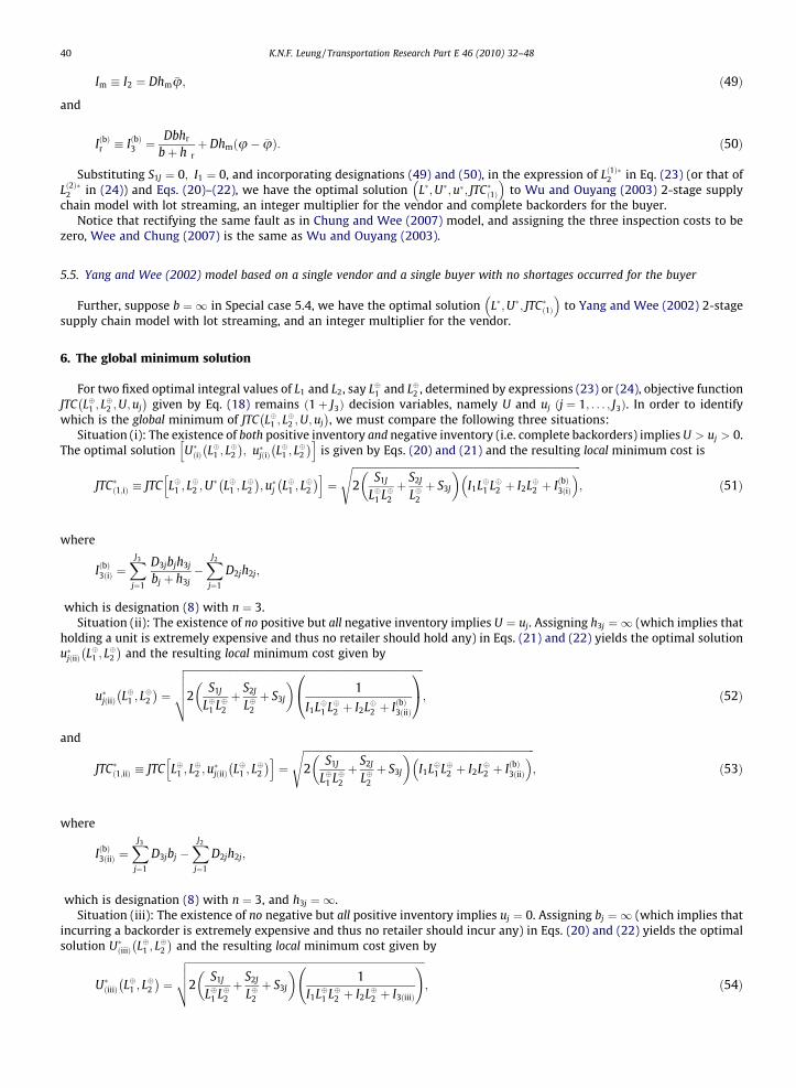
40 K.N.F. Leung / Transportation Research Part E 46 (2010) 32–48
Im � I2 ¼ Dhm �u; ð49Þ
and
IðbÞr � IðbÞ3 ¼Dbhr
bþ h rþ Dhmðu� �uÞ: ð50Þ
Substituting S1J ¼ 0; I1 ¼ 0, and incorporating designations (49) and (50), in the expression of Lð1Þ�2 in Eq. (23) (or that ofLð2Þ�2 in (24)) and Eqs. (20)–(22), we have the optimal solution L�;U�;u�; JTC�ð1Þ
� �to Wu and Ouyang (2003) 2-stage supply
chain model with lot streaming, an integer multiplier for the vendor and complete backorders for the buyer.Notice that rectifying the same fault as in Chung and Wee (2007) model, and assigning the three inspection costs to be
zero, Wee and Chung (2007) is the same as Wu and Ouyang (2003).
5.5. Yang and Wee (2002) model based on a single vendor and a single buyer with no shortages occurred for the buyer
Further, suppose b ¼ 1 in Special case 5.4, we have the optimal solution L�;U�; JTC�ð1Þ� �
to Yang and Wee (2002) 2-stagesupply chain model with lot streaming, and an integer multiplier for the vendor.
6. The global minimum solution
For two fixed optimal integral values of L1 and L2, say L�1 and L�2 , determined by expressions (23) or (24), objective functionJTC L�1 ; L
�2 ;U;uj
� �given by Eq. (18) remains ð1þ J3Þ decision variables, namely U and uj ðj ¼ 1; . . . ; J3Þ. In order to identify
which is the global minimum of JTC L�1 ; L�2 ;U; uj
� �, we must compare the following three situations:
Situation (i): The existence of both positive inventory and negative inventory (i.e. complete backorders) implies U > uj > 0.The optimal solution U�ðiÞ L�1 ; L
�2
� �; u�jðiÞ L�1 ; L
�2
� �h iis given by Eqs. (20) and (21) and the resulting local minimum cost is
JTC�ð1;iÞ � JTC L�1 ; L�2 ;U
� L�1 ; L�2
� �;u�j L�1 ; L
�2
� �h i¼
ffiffiffiffiffiffiffiffiffiffiffiffiffiffiffiffiffiffiffiffiffiffiffiffiffiffiffiffiffiffiffiffiffiffiffiffiffiffiffiffiffiffiffiffiffiffiffiffiffiffiffiffiffiffiffiffiffiffiffiffiffiffiffiffiffiffiffiffiffiffiffiffiffiffiffiffiffiffiffiffiffiffiffiffiffiffiffiffiffiffi2
S1J
L�1 L�2þ S2J
L�2þ S3J
� �I1L�1 L�2 þ I2L�2 þ IðbÞ3ðiÞ
� �s; ð51Þ
where
IðbÞ3ðiÞ ¼XJ3
j¼1
D3jbjh3j
bj þ h3j�XJ2
j¼1
D2jh2j;
which is designation (8) with n ¼ 3.Situation (ii): The existence of no positive but all negative inventory implies U ¼ uj. Assigning h3j ¼ 1 (which implies that
holding a unit is extremely expensive and thus no retailer should hold any) in Eqs. (21) and (22) yields the optimal solutionu�jðiiÞ L�1 ; L
�2
� �and the resulting local minimum cost given by
u�jðiiÞ L�1 ; L�2
� �¼
ffiffiffiffiffiffiffiffiffiffiffiffiffiffiffiffiffiffiffiffiffiffiffiffiffiffiffiffiffiffiffiffiffiffiffiffiffiffiffiffiffiffiffiffiffiffiffiffiffiffiffiffiffiffiffiffiffiffiffiffiffiffiffiffiffiffiffiffiffiffiffiffiffiffiffiffiffiffiffiffiffiffiffiffiffiffiffiffiffiffiffiffiffi2
S1J
L�1 L�2þ S2J
L�2þ S3J
� �1
I1L�1 L�2 þ I2L�2 þ IðbÞ3ðiiÞ
0@
1A
vuuut ; ð52Þ
and
JTC�ð1;iiÞ � JTC L�1 ; L�2 ;u
�jðiiÞ L�1 ; L
�2
� �h i¼
ffiffiffiffiffiffiffiffiffiffiffiffiffiffiffiffiffiffiffiffiffiffiffiffiffiffiffiffiffiffiffiffiffiffiffiffiffiffiffiffiffiffiffiffiffiffiffiffiffiffiffiffiffiffiffiffiffiffiffiffiffiffiffiffiffiffiffiffiffiffiffiffiffiffiffiffiffiffiffiffiffiffiffiffiffiffiffiffiffiffiffi2
S1J
L�1 L�2þ S2J
L�2þ S3J
� �I1L�1 L�2 þ I2L�2 þ IðbÞ3ðiiÞ
� �s; ð53Þ
where
IðbÞ3ðiiÞ ¼XJ3
j¼1
D3jbj �XJ2
j¼1
D2jh2j;
which is designation (8) with n ¼ 3, and h3j ¼ 1.Situation (iii): The existence of no negative but all positive inventory implies uj ¼ 0. Assigning bj ¼ 1 (which implies that
incurring a backorder is extremely expensive and thus no retailer should incur any) in Eqs. (20) and (22) yields the optimalsolution U�ðiiiÞ L�1 ; L
�2
� �and the resulting local minimum cost given by
U�ðiiiÞ L�1 ; L�2
� �¼
ffiffiffiffiffiffiffiffiffiffiffiffiffiffiffiffiffiffiffiffiffiffiffiffiffiffiffiffiffiffiffiffiffiffiffiffiffiffiffiffiffiffiffiffiffiffiffiffiffiffiffiffiffiffiffiffiffiffiffiffiffiffiffiffiffiffiffiffiffiffiffiffiffiffiffiffiffiffiffiffiffiffiffiffiffiffiffiffiffiffiffiffiffi2
S1J
L�1 L�2þ S2J
L�2þ S3J
� �1
I1L�1 L�2 þ I2L�2 þ I3ðiiiÞ
!vuut ; ð54Þ
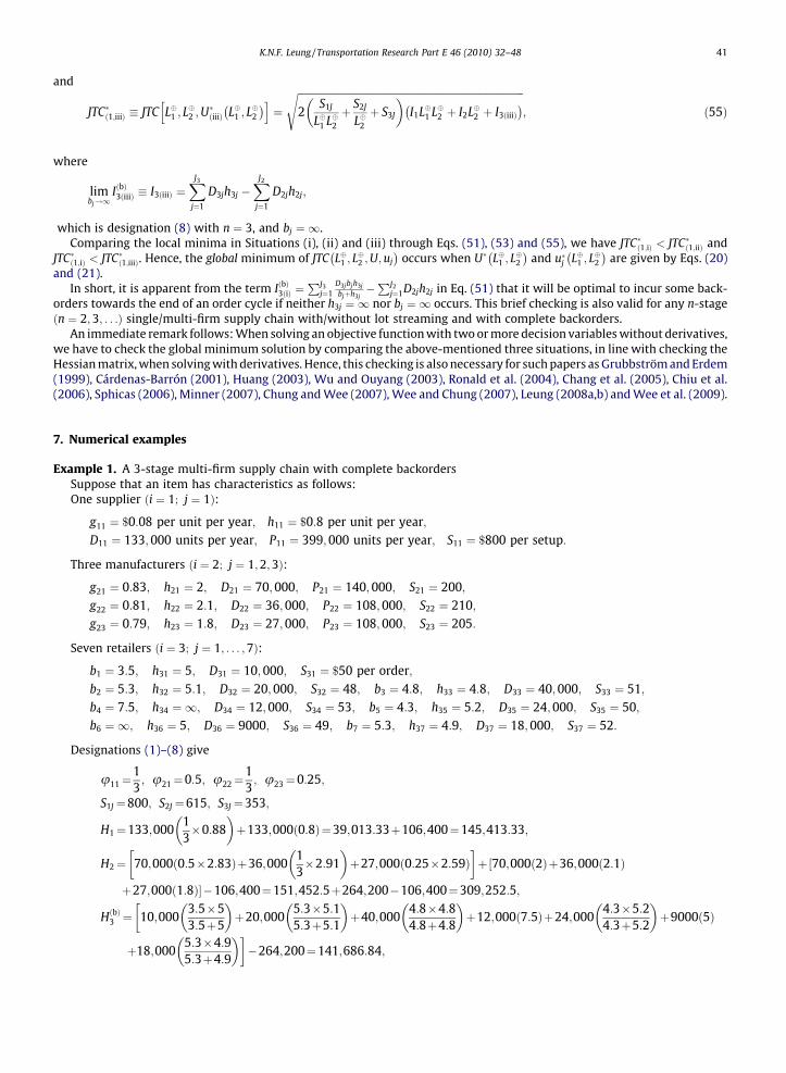
K.N.F. Leung / Transportation Research Part E 46 (2010) 32–48 41
and
JTC�ð1;iiiÞ � JTC L�1 ; L�2 ;U
�ðiiiÞ L�1 ; L
�2
� �h i¼
ffiffiffiffiffiffiffiffiffiffiffiffiffiffiffiffiffiffiffiffiffiffiffiffiffiffiffiffiffiffiffiffiffiffiffiffiffiffiffiffiffiffiffiffiffiffiffiffiffiffiffiffiffiffiffiffiffiffiffiffiffiffiffiffiffiffiffiffiffiffiffiffiffiffiffiffiffiffiffiffiffiffiffiffiffiffiffiffiffiffi2
S1J
L�1 L�2þ S2J
L�2þ S3J
� �I1L�1 L�2 þ I2L�2 þ I3ðiiiÞ� �s
; ð55Þ
where
limbj!1
IðbÞ3ðiiiÞ � I3ðiiiÞ ¼XJ3
j¼1
D3jh3j �XJ2
j¼1
D2jh2j;
which is designation (8) with n ¼ 3, and bj ¼ 1.Comparing the local minima in Situations (i), (ii) and (iii) through Eqs. (51), (53) and (55), we have JTC�ð1;iÞ < JTC�ð1;iiÞ and
JTC�ð1;iÞ < JTC�ð1;iiiÞ. Hence, the global minimum of JTC L�1 ; L�2 ;U;uj
� �occurs when U� L�1 ; L
�2
� �and u�j L�1 ; L
�2
� �are given by Eqs. (20)
and (21).In short, it is apparent from the term IðbÞ3ðiÞ ¼
PJ3j¼1
D3jbjh3j
bjþh3j�PJ2
j¼1D2jh2j in Eq. (51) that it will be optimal to incur some back-orders towards the end of an order cycle if neither h3j ¼ 1 nor bj ¼ 1 occurs. This brief checking is also valid for any n-stageðn ¼ 2;3; . . .Þ single/multi-firm supply chain with/without lot streaming and with complete backorders.
An immediate remark follows: When solving an objective function with two or more decision variables without derivatives,we have to check the global minimum solution by comparing the above-mentioned three situations, in line with checking theHessian matrix, when solving with derivatives. Hence, this checking is also necessary for such papers as Grubbström and Erdem(1999), Cárdenas-Barrón (2001), Huang (2003), Wu and Ouyang (2003), Ronald et al. (2004), Chang et al. (2005), Chiu et al.(2006), Sphicas (2006), Minner (2007), Chung and Wee (2007), Wee and Chung (2007), Leung (2008a,b) and Wee et al. (2009).
7. Numerical examples
Example 1. A 3-stage multi-firm supply chain with complete backordersSuppose that an item has characteristics as follows:One supplier ði ¼ 1; j ¼ 1Þ:
g11 ¼ $0:08 per unit per year; h11 ¼ $0:8 per unit per year;D11 ¼ 133; 000 units per year; P11 ¼ 399;000 units per year; S11 ¼ $800 per setup:
Three manufacturers ði ¼ 2; j ¼ 1;2;3Þ:
g21 ¼ 0:83; h21 ¼ 2; D21 ¼ 70;000; P21 ¼ 140; 000; S21 ¼ 200;g22 ¼ 0:81; h22 ¼ 2:1; D22 ¼ 36;000; P22 ¼ 108; 000; S22 ¼ 210;g23 ¼ 0:79; h23 ¼ 1:8; D23 ¼ 27;000; P23 ¼ 108; 000; S23 ¼ 205:
Seven retailers ði ¼ 3; j ¼ 1; . . . ;7Þ:
b1 ¼ 3:5; h31 ¼ 5; D31 ¼ 10; 000; S31 ¼ $50 per order;b2 ¼ 5:3; h32 ¼ 5:1; D32 ¼ 20;000; S32 ¼ 48; b3 ¼ 4:8; h33 ¼ 4:8; D33 ¼ 40;000; S33 ¼ 51;b4 ¼ 7:5; h34 ¼ 1; D34 ¼ 12;000; S34 ¼ 53; b5 ¼ 4:3; h35 ¼ 5:2; D35 ¼ 24;000; S35 ¼ 50;b6 ¼ 1; h36 ¼ 5; D36 ¼ 9000; S36 ¼ 49; b7 ¼ 5:3; h37 ¼ 4:9; D37 ¼ 18; 000; S37 ¼ 52:
Designations (1)–(8) give
u11¼13; u21¼0:5; u22¼
13; u23¼0:25;
S1J ¼800; S2J ¼615; S3J ¼353;
H1¼133;00013�0:88
� �þ133;000ð0:8Þ¼39;013:33þ106;400¼145;413:33;
H2¼ 70;000ð0:5�2:83Þþ36;00013�2:91
� �þ27;000ð0:25�2:59Þ
þ½70;000ð2Þþ36;000ð2:1Þ
þ27;000ð1:8Þ��106;400¼151;452:5þ264;200�106;400¼309;252:5;
HðbÞ3 ¼ 10;0003:5�53:5þ5
� �þ20;000
5:3�5:15:3þ5:1
� �þ40;000
4:8�4:84:8þ4:8
� �þ12;000ð7:5Þþ24;000
4:3�5:24:3þ5:2
� �þ9000ð5Þ
þ18;0005:3�4:95:3þ4:9
� ��264;200¼141;686:84;
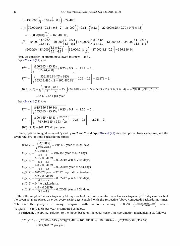
42 K.N.F. Leung / Transportation Research Part E 46 (2010) 32–48
I1¼133;00013�0:08þ2
3�0:8
� �¼74;480;
I2¼ 70;000ð0:5�0:83þ0:5�2Þþ36;00013�0:81þ2
3�2:1
� �þ27;000ð0:25�0:79þ0:75�1:8Þ
�133;000ð0:8Þ 13
� �¼165;485:83;
IðbÞ3 ¼ 10;0003:5�53:5þ5
� �þ20;000
5:3�5:15:3þ5:1
� �þ40;000
4:8�4:84:8þ4:8
� �þ12;000ð7:5Þþ24;000
4:3�5:24:3þ5:2
� �
þ9000ð5Þþ18;0005:3�4:95:3þ4:9
� �� 36;000ð2:1Þ 1
3
� �þ27;000ð1:8Þð0:5Þ
¼356;386:84:
First, we consider lot streaming allowed in stages 1 and 2:Eqs. (23) and (22) give
Lð1Þ�1 ¼
ffiffiffiffiffiffiffiffiffiffiffiffiffiffiffiffiffiffiffiffiffiffiffiffiffiffiffiffiffiffiffiffiffiffiffiffiffiffiffiffiffiffiffiffiffiffiffiffiffiffiffiffiffiffi800ð165;485:83Þ
615ð74;480Þ þ 0:25
sþ 0:5
$ %¼ b2:27c ¼ 2;
Lð1Þ�2 ¼
ffiffiffiffiffiffiffiffiffiffiffiffiffiffiffiffiffiffiffiffiffiffiffiffiffiffiffiffiffiffiffiffiffiffiffiffiffiffiffiffiffiffiffiffiffiffiffiffiffiffiffiffiffiffiffiffiffiffiffiffiffiffiffiffiffiffiffiffiffiffiffiffiffiffiffiffiffiffiffiffiffiffiffiffi356;386:84 800
2 þ 615� �
353ð74;480� 2þ 165;485:83Þ þ 0:25
sþ 0:5
66647775 ¼ b2:37c ¼ 2;
JTC�ð1Þð2;2Þ ¼
ffiffiffiffiffiffiffiffiffiffiffiffiffiffiffiffiffiffiffiffiffiffiffiffiffiffiffiffiffiffiffiffiffiffiffiffiffiffiffiffiffiffiffiffiffiffiffiffiffiffiffiffiffiffiffiffiffiffiffiffiffiffiffiffiffiffiffiffiffiffiffiffiffiffiffiffiffiffiffiffiffiffiffiffiffiffiffiffiffiffiffiffiffiffiffiffiffiffiffiffiffiffiffiffiffiffiffiffiffiffiffiffiffiffiffiffiffiffiffiffiffiffiffiffiffiffiffiffiffiffiffiffiffiffiffiffiffiffiffiffiffiffiffiffiffiffiffi2
8004þ 615
2þ 353
� �ð74;480� 4þ 165;485:83� 2þ 356;386:84Þ
s¼
ffiffiffiffiffiffiffiffiffiffiffiffiffiffiffiffiffiffiffiffiffiffiffiffiffiffiffiffiffiffiffiffiffiffiffiffiffiffiffiffiffiffiffiffiffiffi2ð860:5Þð985;278:5Þ
p¼ $41;178:44 per year:
Eqs. (24) and (22) give
Lð2Þ�2 ¼
ffiffiffiffiffiffiffiffiffiffiffiffiffiffiffiffiffiffiffiffiffiffiffiffiffiffiffiffiffiffiffiffiffiffiffiffiffiffiffiffiffiffiffiffiffiffiffiffiffiffiffiffiffiffi615ð356;386:84Þ353ð165;485:83Þ þ 0:25
sþ 0:5
$ %¼ b2:50c ¼ 2;
Lð2Þ�1 ¼
ffiffiffiffiffiffiffiffiffiffiffiffiffiffiffiffiffiffiffiffiffiffiffiffiffiffiffiffiffiffiffiffiffiffiffiffiffiffiffiffiffiffiffiffiffiffiffiffiffiffiffiffiffiffiffiffiffiffiffiffiffiffiffiffiffiffiffiffiffiffiffiffiffiffiffiffi800ð165;485:83þ 356;386:84
2 Þ74;480ð615þ 353� 2Þ þ 0:25
sþ 0:5
66647775 ¼ b2:24c ¼ 2;
JTC�ð1Þð2;2Þ ¼ $41;178:44 per year:
Hence, optimal integral values of L1 and L2 are 2 and 2, and Eqs. (20) and (21) give the optimal basic cycle time, and theseven retailers’ optimal backordering times:
U�ð2;2Þ ¼
ffiffiffiffiffiffiffiffiffiffiffiffiffiffiffiffiffiffiffiffiffiffiffiffi2ð860:5Þ
985;278:5
s¼ 0:04179 year ffi 15:25 days;
u�1ð2;2Þ ¼5� 0:04179
3:5þ 5¼ 0:02458 year ffi 8:97 days;
u�2ð2;2Þ ¼5:1� 0:04179
5:3þ 5:1¼ 0:02049 year ffi 7:48 days;
u�3ð2;2Þ ¼4:8� 0:04179
4:8þ 4:8¼ 0:020895 year ffi 7:63 days;
u�4ð2;2Þ ¼ 0:06073 year ffi 22:17 days ðall backordersÞ;
u�5ð2;2Þ ¼5:2� 0:04179
4:3þ 5:2¼ 0:02287 year ffi 8:35 days;
u�6ð2;2Þ ¼ 0 ðno backordersÞ;
u�7ð2;2Þ ¼4:9� 0:04179
5:3þ 4:9¼ 0:02008 year ffi 7:33 days:
Thus, the supplier fixes a setup every 61 days, each of the three manufacturers fixes a setup every 30.5 days and each ofthe seven retailers places an order every 15.25 days, coupled with the respective (above-computed) backordering times.
Note that the yearly cost saving, compared with no lot streaming, is 8.59% ¼ 45;049:66�41;178:4445;049:66
� �, where
JTC�ð0Þð2;1Þ ¼ $45;049:66 per year is computed as below.In particular, the optimal solution to the model based on the equal-cycle-time coordination mechanism is as follows:
JTC�ð1Þð1;1Þ ¼ffiffiffiffiffiffiffiffiffiffiffiffiffiffiffiffiffiffiffiffiffiffiffiffiffiffiffiffiffiffiffiffiffiffiffiffiffiffiffiffiffiffiffiffiffiffiffiffiffiffiffiffiffiffiffiffiffiffiffiffiffiffiffiffiffiffiffiffiffiffiffiffiffiffiffiffiffiffiffiffiffiffiffiffiffiffiffiffiffiffiffiffiffiffiffiffiffiffiffiffiffiffiffiffiffiffiffiffiffiffiffiffiffiffiffiffiffiffiffiffiffiffiffiffiffiffiffi2ð800þ 615þ 353Þð74;480þ 165;485:83þ 356;386:84Þ
p¼
ffiffiffiffiffiffiffiffiffiffiffiffiffiffiffiffiffiffiffiffiffiffiffiffiffiffiffiffiffiffiffiffiffiffiffiffiffiffiffiffiffiffiffiffiffiffiffiffi2ð1768Þð596;352:67Þ
p¼ $45;920:62 per year;
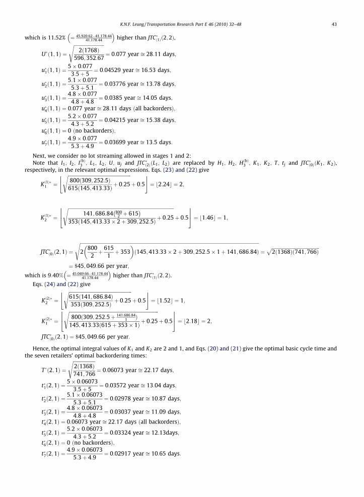
K.N.F. Leung / Transportation Research Part E 46 (2010) 32–48 43
which is 11.52% ¼ 45;920:62�41;178:4441;178:44
� �higher than JTC�ð1Þð2;2Þ,
U�ð1;1Þ ¼
ffiffiffiffiffiffiffiffiffiffiffiffiffiffiffiffiffiffiffiffiffiffiffiffiffiffi2ð1768Þ
596;352:67
s¼ 0:077 year ffi 28:11 days;
u�1ð1;1Þ ¼5� 0:077
3:5þ 5¼ 0:04529 year ffi 16:53 days;
u�2ð1;1Þ ¼5:1� 0:077
5:3þ 5:1¼ 0:03776 year ffi 13:78 days;
u�3ð1;1Þ ¼4:8� 0:077
4:8þ 4:8¼ 0:0385 year ffi 14:05 days;
u�4ð1;1Þ ¼ 0:077 year ffi 28:11 days ðall backordersÞ;
u�5ð1;1Þ ¼5:2� 0:077
4:3þ 5:2¼ 0:04215 year ffi 15:38 days;
u�6ð1;1Þ ¼ 0 ðno backordersÞ;
u�7ð1;1Þ ¼4:9� 0:077
5:3þ 4:9¼ 0:03699 year ffi 13:5 days:
Next, we consider no lot streaming allowed in stages 1 and 2:Note that I1; I2; IðbÞ3 ; L1; L2; U; uj and JTC�ð2ÞðL1; L2Þ are replaced by H1; H2; HðbÞ3 ; K1; K2; T; tj and JTC�ð0ÞðK1; K2Þ,
respectively, in the relevant optimal expressions. Eqs. (23) and (22) give
Kð1Þ�1 ¼
ffiffiffiffiffiffiffiffiffiffiffiffiffiffiffiffiffiffiffiffiffiffiffiffiffiffiffiffiffiffiffiffiffiffiffiffiffiffiffiffiffiffiffiffiffiffiffiffiffiffiffiffiffiffi800ð309;252:5Þ
615ð145;413:33Þ þ 0:25
sþ 0:5
$ %¼ b2:24c ¼ 2;
Kð1Þ�2 ¼
ffiffiffiffiffiffiffiffiffiffiffiffiffiffiffiffiffiffiffiffiffiffiffiffiffiffiffiffiffiffiffiffiffiffiffiffiffiffiffiffiffiffiffiffiffiffiffiffiffiffiffiffiffiffiffiffiffiffiffiffiffiffiffiffiffiffiffiffiffiffiffiffiffiffiffiffiffiffiffiffiffiffiffiffiffiffiffiffiffiffiffi141;686:84 800
2 þ 615� �
353ð145;413:33� 2þ 309;252:5Þ þ 0:25
sþ 0:5
66647775 ¼ b1:46c ¼ 1;
JTC�ð0Þð2;1Þ ¼
ffiffiffiffiffiffiffiffiffiffiffiffiffiffiffiffiffiffiffiffiffiffiffiffiffiffiffiffiffiffiffiffiffiffiffiffiffiffiffiffiffiffiffiffiffiffiffiffiffiffiffiffiffiffiffiffiffiffiffiffiffiffiffiffiffiffiffiffiffiffiffiffiffiffiffiffiffiffiffiffiffiffiffiffiffiffiffiffiffiffiffiffiffiffiffiffiffiffiffiffiffiffiffiffiffiffiffiffiffiffiffiffiffiffiffiffiffiffiffiffiffiffiffiffiffiffiffiffiffiffiffiffiffiffiffiffiffiffiffiffiffiffiffiffiffiffiffiffiffiffiffiffiffiffi2
8002þ 615
1þ 353
� �ð145;413:33� 2þ 309;252:5� 1þ 141;686:84Þ
s¼
ffiffiffiffiffiffiffiffiffiffiffiffiffiffiffiffiffiffiffiffiffiffiffiffiffiffiffiffiffiffiffiffiffiffiffiffiffiffiffiffiffi2ð1368Þð741;766Þ
p¼ $45;049:66 per year;� �
which is 9:40% ¼ 45;049:66�41;178:4441;178:44 higher than JTC�ð1Þð2;2Þ.
Eqs. (24) and (22) give
Kð2Þ�2 ¼
ffiffiffiffiffiffiffiffiffiffiffiffiffiffiffiffiffiffiffiffiffiffiffiffiffiffiffiffiffiffiffiffiffiffiffiffiffiffiffiffiffiffiffiffiffiffiffiffiffiffiffiffiffiffi615ð141;686:84Þ353ð309;252:5Þ þ 0:25
sþ 0:5
$ %¼ b1:52c ¼ 1;
Kð2Þ�1 ¼
ffiffiffiffiffiffiffiffiffiffiffiffiffiffiffiffiffiffiffiffiffiffiffiffiffiffiffiffiffiffiffiffiffiffiffiffiffiffiffiffiffiffiffiffiffiffiffiffiffiffiffiffiffiffiffiffiffiffiffiffiffiffiffiffiffiffiffiffiffiffiffiffiffiffiffiffiffi800ð309;252:5þ 141;686:84
1 Þ145;413:33ð615þ 353� 1Þ þ 0:25
sþ 0:5
66647775 ¼ b2:18c ¼ 2;
JTC�ð0Þð2;1Þ ¼ $45; 049:66 per year:
Hence, the optimal integral values of K1 and K2 are 2 and 1, and Eqs. (20) and (21) give the optimal basic cycle time andthe seven retailers’ optimal backordering times:
T�ð2;1Þ ¼
ffiffiffiffiffiffiffiffiffiffiffiffiffiffiffiffiffiffiffi2ð1368Þ741;766
s¼ 0:06073 year ffi 22:17 days;
t�1ð2;1Þ ¼5� 0:06073
3:5þ 5¼ 0:03572 year ffi 13:04 days;
t�2ð2;1Þ ¼5:1� 0:06073
5:3þ 5:1¼ 0:02978 year ffi 10:87 days;
t�3ð2;1Þ ¼4:8� 0:06073
4:8þ 4:8¼ 0:03037 year ffi 11:09 days;
t�4ð2;1Þ ¼ 0:06073 year ffi 22:17 days ðall backordersÞ;
t�5ð2;1Þ ¼5:2� 0:06073
4:3þ 5:2¼ 0:03324 year ffi 12:13days;
t�6ð2;1Þ ¼ 0 ðno backordersÞ;
t�7ð2;1Þ ¼4:9� 0:06073
5:3þ 4:9¼ 0:02917 year ffi 10:65 days:
44 K.N.F. Leung / Transportation Research Part E 46 (2010) 32–48
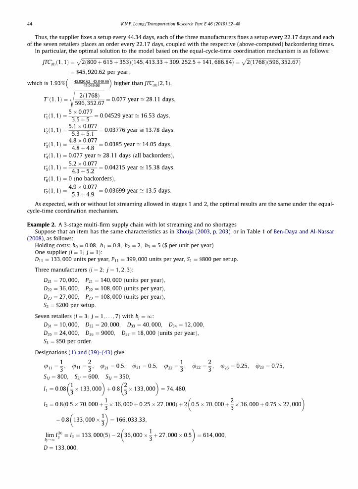
Thus, the supplier fixes a setup every 44.34 days, each of the three manufacturers fixes a setup every 22.17 days and eachof the seven retailers places an order every 22.17 days, coupled with the respective (above-computed) backordering times.
In particular, the optimal solution to the model based on the equal-cycle-time coordination mechanism is as follows:
JTC�ð0Þð1;1Þ ¼ffiffiffiffiffiffiffiffiffiffiffiffiffiffiffiffiffiffiffiffiffiffiffiffiffiffiffiffiffiffiffiffiffiffiffiffiffiffiffiffiffiffiffiffiffiffiffiffiffiffiffiffiffiffiffiffiffiffiffiffiffiffiffiffiffiffiffiffiffiffiffiffiffiffiffiffiffiffiffiffiffiffiffiffiffiffiffiffiffiffiffiffiffiffiffiffiffiffiffiffiffiffiffiffiffiffiffiffiffiffiffiffiffiffiffiffiffiffiffiffiffiffiffiffiffiffiffiffiffiffiffiffiffiffi2ð800þ 615þ 353Þð145;413:33þ 309;252:5þ 141;686:84Þ
p¼
ffiffiffiffiffiffiffiffiffiffiffiffiffiffiffiffiffiffiffiffiffiffiffiffiffiffiffiffiffiffiffiffiffiffiffiffiffiffiffiffiffiffiffiffiffiffiffiffi2ð1768Þð596;352:67Þ
p¼ $45;920:62 per year;
which is 1:93% ¼ 45;920:62�45;049:6645;049:66
� �higher than JTC�ð0Þð2;1Þ,
T�ð1;1Þ ¼
ffiffiffiffiffiffiffiffiffiffiffiffiffiffiffiffiffiffiffiffiffiffiffiffiffiffi2ð1768Þ
596;352:67
s¼ 0:077 year ffi 28:11 days;
t�1ð1;1Þ ¼5� 0:077
3:5þ 5¼ 0:04529 year ffi 16:53 days;
t�2ð1;1Þ ¼5:1� 0:077
5:3þ 5:1¼ 0:03776 year ffi 13:78 days;
t�3ð1;1Þ ¼4:8� 0:077
4:8þ 4:8¼ 0:0385 year ffi 14:05 days;
t�4ð1;1Þ ¼ 0:077 year ffi 28:11 days ðall backordersÞ;
t�5ð1;1Þ ¼5:2� 0:077
4:3þ 5:2¼ 0:04215 year ffi 15:38 days;
t�6ð1;1Þ ¼ 0 ðno backordersÞ;
t�7ð1;1Þ ¼4:9� 0:077
5:3þ 4:9¼ 0:03699 year ffi 13:5 days:
As expected, with or without lot streaming allowed in stages 1 and 2, the optimal results are the same under the equal-cycle-time coordination mechanism.
Example 2. A 3-stage multi-firm supply chain with lot streaming and no shortagesSuppose that an item has the same characteristics as in Khouja (2003, p. 203), or in Table 1 of Ben-Daya and Al-Nassar
(2008), as follows:Holding costs: h0 ¼ 0:08; h1 ¼ 0:8; h2 ¼ 2; h3 ¼ 5 ($ per unit per year)One supplier ði ¼ 1; j ¼ 1Þ:D11 ¼ 133;000 units per year, P11 ¼ 399;000 units per year, S1 ¼ $800 per setup.
Three manufacturers ði ¼ 2; j ¼ 1;2;3Þ:
D21 ¼ 70;000; P21 ¼ 140;000 ðunits per yearÞ;D22 ¼ 36; 000; P22 ¼ 108;000 ðunits per yearÞ;D23 ¼ 27; 000; P23 ¼ 108;000 ðunits per yearÞ;S2 ¼ $200 per setup:
Seven retailers ði ¼ 3; j ¼ 1; . . . ;7Þ with bj ¼ 1:
D31 ¼ 10;000; D32 ¼ 20; 000; D33 ¼ 40; 000; D34 ¼ 12; 000;D35 ¼ 24; 000; D36 ¼ 9000; D37 ¼ 18;000 ðunits per yearÞ;S3 ¼ $50 per order:
Designations (1) and (39)–(43) give
u11 ¼13; �u11 ¼
23; u21 ¼ 0:5; �u21 ¼ 0:5; u22 ¼
13; �u22 ¼
23; u23 ¼ 0:25; �u23 ¼ 0:75;
S1J ¼ 800; S2J ¼ 600; S3J ¼ 350;
I1 ¼ 0:0813� 133;000
� �þ 0:8
23� 133; 000
� �¼ 74;480;
I2 ¼ 0:8ð0:5� 70;000þ 13� 36; 000þ 0:25� 27;000Þ þ 2 0:5� 70; 000þ 2
3� 36;000þ 0:75� 27;000
� �
� 0:8 133; 000� 13
� �¼ 166;033:33;
limbj!1
IðbÞ3 � I3 ¼ 133;000ð5Þ � 2 36;000� 13þ 27;000� 0:5
� �¼ 614; 000;
D ¼ 133;000:
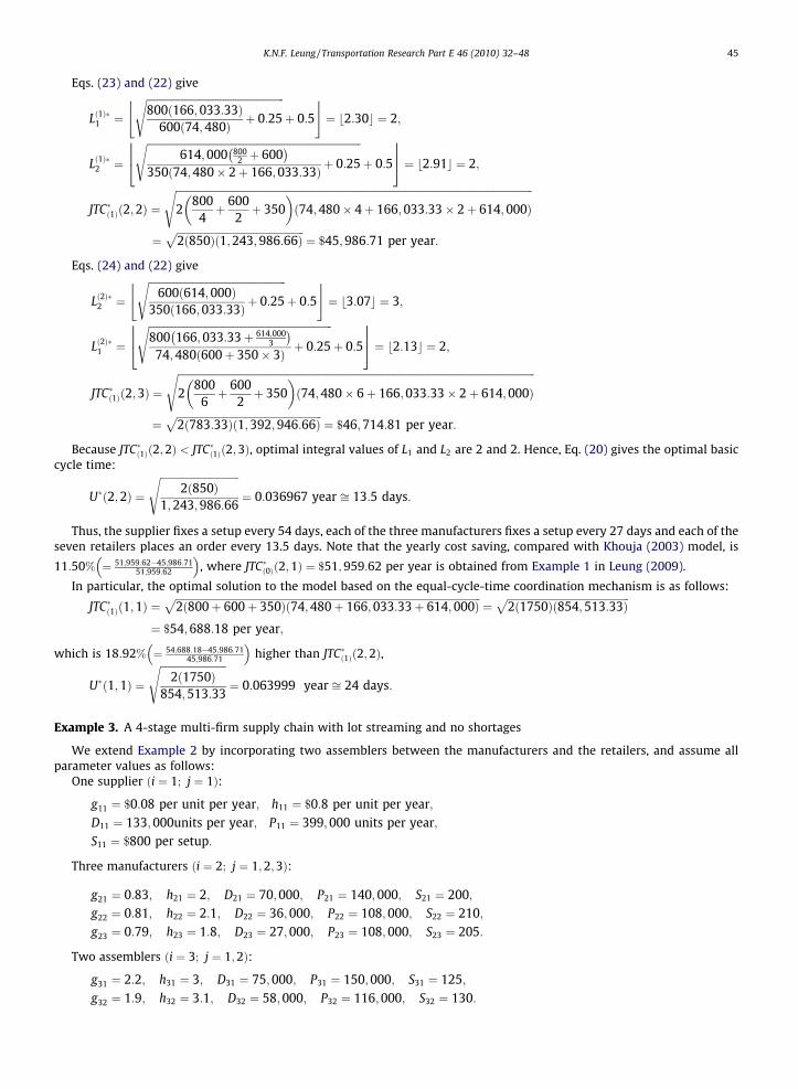
K.N.F. Leung / Transportation Research Part E 46 (2010) 32–48 45
Eqs. (23) and (22) give
Lð1Þ�1 ¼
ffiffiffiffiffiffiffiffiffiffiffiffiffiffiffiffiffiffiffiffiffiffiffiffiffiffiffiffiffiffiffiffiffiffiffiffiffiffiffiffiffiffiffiffiffiffiffiffiffiffiffiffiffiffi800ð166; 033:33Þ
600ð74;480Þ þ 0:25
sþ 0:5
$ %¼ b2:30c ¼ 2;
Lð1Þ�2 ¼
ffiffiffiffiffiffiffiffiffiffiffiffiffiffiffiffiffiffiffiffiffiffiffiffiffiffiffiffiffiffiffiffiffiffiffiffiffiffiffiffiffiffiffiffiffiffiffiffiffiffiffiffiffiffiffiffiffiffiffiffiffiffiffiffiffiffiffiffiffiffiffiffiffiffiffiffiffiffiffiffiffiffiffiffi614;000 800
2 þ 600� �
350ð74;480� 2þ 166;033:33Þ þ 0:25
sþ 0:5
66647775 ¼ b2:91c ¼ 2;
JTC�ð1Þð2;2Þ ¼
ffiffiffiffiffiffiffiffiffiffiffiffiffiffiffiffiffiffiffiffiffiffiffiffiffiffiffiffiffiffiffiffiffiffiffiffiffiffiffiffiffiffiffiffiffiffiffiffiffiffiffiffiffiffiffiffiffiffiffiffiffiffiffiffiffiffiffiffiffiffiffiffiffiffiffiffiffiffiffiffiffiffiffiffiffiffiffiffiffiffiffiffiffiffiffiffiffiffiffiffiffiffiffiffiffiffiffiffiffiffiffiffiffiffiffiffiffiffiffiffiffiffiffiffiffiffiffiffiffiffiffiffiffiffiffiffiffiffiffiffi2
8004þ 600
2þ 350
� �ð74;480� 4þ 166;033:33� 2þ 614; 000Þ
s
¼ffiffiffiffiffiffiffiffiffiffiffiffiffiffiffiffiffiffiffiffiffiffiffiffiffiffiffiffiffiffiffiffiffiffiffiffiffiffiffiffiffiffiffiffiffiffiffiffiffiffi2ð850Þð1;243;986:66Þ
p¼ $45;986:71 per year:
Eqs. (24) and (22) give
Lð2Þ�2 ¼
ffiffiffiffiffiffiffiffiffiffiffiffiffiffiffiffiffiffiffiffiffiffiffiffiffiffiffiffiffiffiffiffiffiffiffiffiffiffiffiffiffiffiffiffiffiffiffiffiffiffiffiffiffiffi600ð614;000Þ
350ð166;033:33Þ þ 0:25
sþ 0:5
$ %¼ b3:07c ¼ 3;
Lð2Þ�1 ¼
ffiffiffiffiffiffiffiffiffiffiffiffiffiffiffiffiffiffiffiffiffiffiffiffiffiffiffiffiffiffiffiffiffiffiffiffiffiffiffiffiffiffiffiffiffiffiffiffiffiffiffiffiffiffiffiffiffiffiffiffiffiffiffiffiffiffiffiffiffiffiffiffi800 166; 033:33þ 614;000
3
� �74;480ð600þ 350� 3Þ þ 0:25
sþ 0:5
66647775 ¼ b2:13c ¼ 2;
JTC�ð1Þð2;3Þ ¼
ffiffiffiffiffiffiffiffiffiffiffiffiffiffiffiffiffiffiffiffiffiffiffiffiffiffiffiffiffiffiffiffiffiffiffiffiffiffiffiffiffiffiffiffiffiffiffiffiffiffiffiffiffiffiffiffiffiffiffiffiffiffiffiffiffiffiffiffiffiffiffiffiffiffiffiffiffiffiffiffiffiffiffiffiffiffiffiffiffiffiffiffiffiffiffiffiffiffiffiffiffiffiffiffiffiffiffiffiffiffiffiffiffiffiffiffiffiffiffiffiffiffiffiffiffiffiffiffiffiffiffiffiffiffiffiffiffiffiffiffi2
8006þ 600
2þ 350
� �ð74;480� 6þ 166;033:33� 2þ 614;000Þ
s
¼ffiffiffiffiffiffiffiffiffiffiffiffiffiffiffiffiffiffiffiffiffiffiffiffiffiffiffiffiffiffiffiffiffiffiffiffiffiffiffiffiffiffiffiffiffiffiffiffiffiffiffiffiffiffiffiffiffi2ð783:33Þð1;392;946:66Þ
p¼ $46;714:81 per year:
Because JTC�ð1Þð2;2Þ < JTC�ð1Þð2;3Þ, optimal integral values of L1 and L2 are 2 and 2. Hence, Eq. (20) gives the optimal basiccycle time:
U�ð2;2Þ ¼
ffiffiffiffiffiffiffiffiffiffiffiffiffiffiffiffiffiffiffiffiffiffiffiffiffiffiffiffiffiffiffi2ð850Þ
1;243;986:66
s¼ 0:036967 year ffi 13:5 days:
Thus, the supplier fixes a setup every 54 days, each of the three manufacturers fixes a setup every 27 days and each of theseven retailers places an order every 13.5 days. Note that the yearly cost saving, compared with Khouja (2003) model, is
11:50% ¼ 51;959:62�45;986:7151;959:62
� �, where JTC�ð0Þð2;1Þ ¼ $51;959:62 per year is obtained from Example 1 in Leung (2009).
In particular, the optimal solution to the model based on the equal-cycle-time coordination mechanism is as follows:
JTC�ð1Þð1;1Þ ¼ffiffiffiffiffiffiffiffiffiffiffiffiffiffiffiffiffiffiffiffiffiffiffiffiffiffiffiffiffiffiffiffiffiffiffiffiffiffiffiffiffiffiffiffiffiffiffiffiffiffiffiffiffiffiffiffiffiffiffiffiffiffiffiffiffiffiffiffiffiffiffiffiffiffiffiffiffiffiffiffiffiffiffiffiffiffiffiffiffiffiffiffiffiffiffiffiffiffiffiffiffiffiffiffiffiffiffiffiffiffiffiffiffiffiffiffiffiffiffiffi2ð800þ 600þ 350Þð74;480þ 166;033:33þ 614; 000Þ
p¼
ffiffiffiffiffiffiffiffiffiffiffiffiffiffiffiffiffiffiffiffiffiffiffiffiffiffiffiffiffiffiffiffiffiffiffiffiffiffiffiffiffiffiffiffiffiffiffiffi2ð1750Þð854;513:33Þ
p¼ $54;688:18 per year;
which is 18:92% ¼ 54;688:18�45;986:7145;986:71
� �higher than JTC�ð1Þð2;2Þ,ffiffiffiffiffiffiffiffiffiffiffiffiffiffiffiffiffiffiffiffiffiffiffiffiffiffis
U�ð1;1Þ ¼ 2ð1750Þ854;513:33
¼ 0:063999 year ffi 24 days:
Example 3. A 4-stage multi-firm supply chain with lot streaming and no shortages
We extend Example 2 by incorporating two assemblers between the manufacturers and the retailers, and assume allparameter values as follows:
One supplier ði ¼ 1; j ¼ 1Þ:
g11 ¼ $0:08 per unit per year; h11 ¼ $0:8 per unit per year;D11 ¼ 133; 000units per year; P11 ¼ 399; 000 units per year;S11 ¼ $800 per setup:
Three manufacturers ði ¼ 2; j ¼ 1;2;3Þ:
g21 ¼ 0:83; h21 ¼ 2; D21 ¼ 70;000; P21 ¼ 140; 000; S21 ¼ 200;g22 ¼ 0:81; h22 ¼ 2:1; D22 ¼ 36;000; P22 ¼ 108; 000; S22 ¼ 210;g23 ¼ 0:79; h23 ¼ 1:8; D23 ¼ 27;000; P23 ¼ 108; 000; S23 ¼ 205:
Two assemblers ði ¼ 3; j ¼ 1;2Þ:
g31 ¼ 2:2; h31 ¼ 3; D31 ¼ 75;000; P31 ¼ 150;000; S31 ¼ 125;g32 ¼ 1:9; h32 ¼ 3:1; D32 ¼ 58;000; P32 ¼ 116;000; S32 ¼ 130:
46 K.N.F. Leung / Transportation Research Part E 46 (2010) 32–48
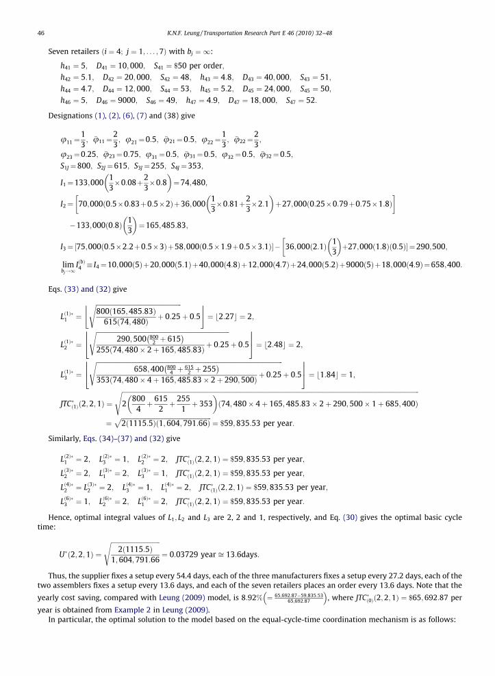
Seven retailers ði ¼ 4; j ¼ 1; . . . ;7Þ with bj ¼ 1:
h41 ¼ 5; D41 ¼ 10;000; S41 ¼ $50 per order;h42 ¼ 5:1; D42 ¼ 20;000; S42 ¼ 48; h43 ¼ 4:8; D43 ¼ 40;000; S43 ¼ 51;h44 ¼ 4:7; D44 ¼ 12; 000; S44 ¼ 53; h45 ¼ 5:2; D45 ¼ 24;000; S45 ¼ 50;h46 ¼ 5; D46 ¼ 9000; S46 ¼ 49; h47 ¼ 4:9; D47 ¼ 18; 000; S47 ¼ 52:
Designations (1), (2), (6), (7) and (38) give
u11¼13; �u11¼
23; u21¼0:5; �u21¼0:5; u22¼
13; �u22¼
23;
u23¼0:25; �u23¼0:75; u31¼0:5; �u31¼0:5; u32¼0:5; �u32¼0:5;S1J¼800; S2J ¼615; S3J¼255; S4J ¼353;
I1¼133;00013�0:08þ2
3�0:8
� �¼74;480;
I2¼ 70;000ð0:5�0:83þ0:5�2Þþ36;00013�0:81þ2
3�2:1
� �þ27;000ð0:25�0:79þ0:75�1:8Þ
�133;000ð0:8Þ 13
� �¼165;485:83;
I3¼½75;000ð0:5�2:2þ0:5�3Þþ58;000ð0:5�1:9þ0:5�3:1Þ�� 36;000ð2:1Þ 13
� �þ27;000ð1:8Þð0:5Þ�¼290;500;
limbj!1
IðbÞ4 � I4¼10;000ð5Þþ20;000ð5:1Þþ40;000ð4:8Þþ12;000ð4:7Þþ24;000ð5:2Þþ9000ð5Þþ18;000ð4:9Þ¼658;400:
Eqs. (33) and (32) give
Lð1Þ�1 ¼
ffiffiffiffiffiffiffiffiffiffiffiffiffiffiffiffiffiffiffiffiffiffiffiffiffiffiffiffiffiffiffiffiffiffiffiffiffiffiffiffiffiffiffiffiffiffiffiffiffiffiffiffiffiffi800ð165;485:83Þ
615ð74;480Þ þ 0:25
sþ 0:5
$ %¼ b2:27c ¼ 2;
Lð1Þ�2 ¼
ffiffiffiffiffiffiffiffiffiffiffiffiffiffiffiffiffiffiffiffiffiffiffiffiffiffiffiffiffiffiffiffiffiffiffiffiffiffiffiffiffiffiffiffiffiffiffiffiffiffiffiffiffiffiffiffiffiffiffiffiffiffiffiffiffiffiffiffiffiffiffiffiffiffiffiffiffiffiffiffiffiffiffiffi290;500 800
2 þ 615� �
255ð74;480� 2þ 165;485:83Þ þ 0:25
sþ 0:5
66647775 ¼ b2:48c ¼ 2;
Lð1Þ�3 ¼
ffiffiffiffiffiffiffiffiffiffiffiffiffiffiffiffiffiffiffiffiffiffiffiffiffiffiffiffiffiffiffiffiffiffiffiffiffiffiffiffiffiffiffiffiffiffiffiffiffiffiffiffiffiffiffiffiffiffiffiffiffiffiffiffiffiffiffiffiffiffiffiffiffiffiffiffiffiffiffiffiffiffiffiffiffiffiffiffiffiffiffiffiffiffiffiffiffiffiffiffiffiffiffiffiffiffiffiffiffiffiffiffiffiffiffiffiffiffi658;400 800
4 þ 6152 þ 255
� �353ð74;480� 4þ 165;485:83� 2þ 290;500Þ þ 0:25
sþ 0:5
66647775 ¼ b1:84c ¼ 1;
JTC�ð1Þð2;2;1Þ ¼
ffiffiffiffiffiffiffiffiffiffiffiffiffiffiffiffiffiffiffiffiffiffiffiffiffiffiffiffiffiffiffiffiffiffiffiffiffiffiffiffiffiffiffiffiffiffiffiffiffiffiffiffiffiffiffiffiffiffiffiffiffiffiffiffiffiffiffiffiffiffiffiffiffiffiffiffiffiffiffiffiffiffiffiffiffiffiffiffiffiffiffiffiffiffiffiffiffiffiffiffiffiffiffiffiffiffiffiffiffiffiffiffiffiffiffiffiffiffiffiffiffiffiffiffiffiffiffiffiffiffiffiffiffiffiffiffiffiffiffiffiffiffiffiffiffiffiffiffiffiffiffiffiffiffiffiffiffiffiffiffiffiffiffiffiffiffiffiffiffiffiffiffiffiffiffiffiffiffiffiffiffiffiffiffiffiffiffiffi2
8004þ 615
2þ 255
1þ 353
� �ð74;480� 4þ 165;485:83� 2þ 290;500� 1þ 685;400Þ
s
¼ffiffiffiffiffiffiffiffiffiffiffiffiffiffiffiffiffiffiffiffiffiffiffiffiffiffiffiffiffiffiffiffiffiffiffiffiffiffiffiffiffiffiffiffiffiffiffiffiffiffiffiffiffiffiffiffiffi2ð1115:5Þð1;604;791:66Þ
p¼ $59;835:53 per year:
Similarly, Eqs. (34)–(37) and (32) give
Lð2Þ�1 ¼ 2; Lð2Þ�3 ¼ 1; Lð2Þ�2 ¼ 2; JTC�ð1Þð2;2;1Þ ¼ $59;835:53 per year;
Lð3Þ�2 ¼ 2; Lð3Þ�1 ¼ 2; Lð3Þ�3 ¼ 1; JTC�ð1Þð2;2;1Þ ¼ $59;835:53 per year;
Lð4Þ�2 ¼ Lð3Þ�2 ¼ 2; Lð4Þ�3 ¼ 1; Lð4Þ�1 ¼ 2; JTC�ð1Þð2;2;1Þ ¼ $59;835:53 per year;
Lð6Þ�3 ¼ 1; Lð6Þ�2 ¼ 2; Lð6Þ�1 ¼ 2; JTC�ð1Þð2;2;1Þ ¼ $59;835:53 per year:
Hence, optimal integral values of L1; L2 and L3 are 2, 2 and 1, respectively, and Eq. (30) gives the optimal basic cycletime:
U�ð2;2;1Þ ¼
ffiffiffiffiffiffiffiffiffiffiffiffiffiffiffiffiffiffiffiffiffiffiffiffiffiffiffiffiffiffiffi2ð1115:5Þ
1;604;791:66
s¼ 0:03729 year ffi 13:6days:
Thus, the supplier fixes a setup every 54.4 days, each of the three manufacturers fixes a setup every 27.2 days, each of thetwo assemblers fixes a setup every 13.6 days, and each of the seven retailers places an order every 13.6 days. Note that the
yearly cost saving, compared with Leung (2009) model, is 8:92% ¼ 65;692:87�59;835:5365;692:87
� �, where JTC�ð0Þð2;2;1Þ ¼ $65;692:87 per
year is obtained from Example 2 in Leung (2009).In particular, the optimal solution to the model based on the equal-cycle-time coordination mechanism is as follows:
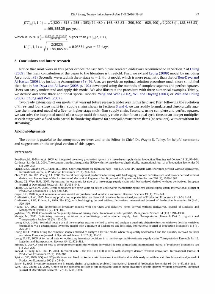
K.N.F. Leung / Transportation Research Part E 46 (2010) 32–48 47
JTC�ð1Þð1;1;1Þ ¼ffiffiffiffiffiffiffiffiffiffiffiffiffiffiffiffiffiffiffiffiffiffiffiffiffiffiffiffiffiffiffiffiffiffiffiffiffiffiffiffiffiffiffiffiffiffiffiffiffiffiffiffiffiffiffiffiffiffiffiffiffiffiffiffiffiffiffiffiffiffiffiffiffiffiffiffiffiffiffiffiffiffiffiffiffiffiffiffiffiffiffiffiffiffiffiffiffiffiffiffiffiffiffiffiffiffiffiffiffiffiffiffiffiffiffiffiffiffiffiffiffiffiffiffiffiffiffiffiffiffiffiffiffiffiffiffiffiffiffiffiffiffiffiffiffiffiffiffiffiffiffiffiffiffiffiffiffiffiffi2ð800þ 615þ 255þ 353Þð74;480þ 165;485:83þ 290;500þ 685;400Þ
p ffiffiffiffiffiffiffiffiffiffiffiffiffiffiffiffiffiffiffiffiffiffiffiffiffiffiffiffiffiffiffiffiffiffiffiffiffiffiffiffiffiffiffiffiffiffiffiffiffiffiffiffiffi2ð2023Þð1;188;865:83Þ
p¼ $69;355:25 per year;
which is 15:91% ¼ 69;355:25�59;835:5359;835:53
� �higher than JTC�ð1Þð2;2;1Þ,
U�ð1;1;1Þ ¼
ffiffiffiffiffiffiffiffiffiffiffiffiffiffiffiffiffiffiffiffiffiffiffiffiffiffiffiffiffiffiffi2ð2023Þ
1;188;865:83
s¼ 0:05834 year ffi 22 days:
8. Conclusions and future research
Notice that most work in this paper echoes the last two future research endeavors recommended in Section 7 of Leung(2009). The main contribution of the paper to the literature is threefold: First, we extend Leung (2009) model by includingAssumption (9). Secondly, we establish the n-stage ðn ¼ 3;4; . . .Þmodel, which is more pragmatic than that of Ben-Daya andAl-Nassar (2008), by including Assumptions (5)–(9). Also, we provide an optimal solution procedure much more simplifiedthat that in Ben-Daya and Al-Nassar (2008, p. 102), developed using the methods of complete squares and perfect squares.Users can easily understand and apply this model. We also illustrate the procedure with three numerical examples. Thirdly,we deduce and solve three additional special models: Yang and Wee (2002), Wu and Ouyang (2003) or Wee and Chung(2007); Chung and Wee (2007).
Two ready extensions of our model that warrant future research endeavors in this field are: First, following the evolutionof three- and four-stage multi-firm supply chains shown in Sections 3 and 4, we can readily formulate and algebraically ana-lyze the integrated model of a five- or higher-stage multi-firm supply chain. Secondly, using complete and perfect squares,we can solve the integrated model of a n-stage multi-firm supply chain either for an equal cycle time, or an integer multiplierat each stage with a fixed ratio partial backordering allowed for some/all downstream firms (or retailers), with or without lotstreaming.
Acknowledgements
The author is grateful to the anonymous reviewer and to the Editor-in-Chief, Dr. Wayne K. Talley, for helpful commentsand suggestions on the original version of this paper.
References
Ben-Daya, M., Al-Nassar, A., 2008. An integrated inventory production system in a three-layer supply chain. Production Planning and Control 19 (2), 97–104.Cárdenas-Barrón, L.E., 2001. The economic production quantity (EPQ) with shortage derived algebraically. International Journal of Production Economics 70
(3), 289–292.Chang, S.K.J., Chuang, P.C.J., Chen, H.J., 2005. Short comments on technical note – the EOQ and EPQ models with shortages derived without derivatives.
International Journal of Production Economics 97 (2), 241–243.Chiu, Y.S.P., Lin, H.D., Cheng, F.T., 2006. Technical note: optimal production lot sizing with backlogging, random defective rate, and rework derived without
derivatives. Proceedings of the Institution of Mechanical Engineers Part B: Journal of Engineering Manufacture 220 (9), 1559–1563.Chung, C.J., Wee, H.M., 2007. Optimizing the economic lot size of a three-stage supply chain with backordered derived without derivatives. European
Journal of Operational Research 183 (2), 933–943.Chung, C.J., Wee, H.M., 2008. Green-component life-cycle value on design and reverse manufacturing in semi-closed supply chain. International Journal of
Production Economics 113 (2), 528–545.Goyal, S.K., 1988. A joint economic-lot-size model for purchaser and vendor: a comment. Decision Sciences 19 (1), 236–241.Grubbström, R.W., 1995. Modeling production opportunities: an historical overview. International Journal of Production Economics 41 (1-3), 1–14.Grubbström, R.W., Erdem, A., 1999. The EOQ with backlogging derived without derivatives. International Journal of Production Economics 59 (1–3),
529–530.Huang, Y.F., 2003. The deterministic inventory models with shortages and defective items derived without derivatives. Journal of Statistics and
Management Systems 6 (2), 171–180.Joglekar, P.N., 1988. Comments on ‘‘A quantity discount pricing model to increase vendor profits”. Management Science 34 (11), 1391–1398.Khouja, M., 2003. Optimizing inventory decisions in a multi-stage multi-customer supply chain. Transportation Research Part E: Logistics and
Transportation Review 39 (3), 193–208.Leung, K.N.F., 2008a. Technical note: a use of the complete squares method to solve and analyze a quadratic objective function with two decision variables
exemplified via a deterministic inventory model with a mixture of backorders and lost sales. International Journal of Production Economics 113 (1),275–281.
Leung, K.N.F., 2008b. Using the complete squares method to analyze a lot size model when the quantity backordered and the quantity received are bothuncertain. European Journal of Operational Research 187 (1), 19–30.
Leung, K.N.F., 2009. A technical note on optimizing inventory decisions in a multi-stage multi-customer supply chain. Transportation Research Part E:Logistics and Transportation Review 45 (4), 572–582.
Minner, S., 2007. A note on how to compute order quantities without derivatives by cost comparisons. International Journal of Production Economics 105(1), 293–296.
Ronald, R., Yang, G.K., Chu, P., 2004. Technical note – the EOQ and EPQ models with shortages derived without derivations. International Journal ofProduction Economics 92 (2), 197–200.
Sphicas, G.P., 2006. EOQ and EPQ with linear and fixed backorder costs: two cases identified and models analyzed without calculus. International Journal ofProduction Economics 100 (1), 59–64.
Sucky, E., 2005. Inventory management in supply chains: a bargaining problem. International Journal of Production Economics 93–94 (1–6), 253–262.Wee, H.M., Chung, C.J., 2007. A note on the economic lot size of the integrated vendor–buyer inventory system derived without derivatives. European
Journal of Operational Research 177 (2), 1289–1293.
48 K.N.F. Leung / Transportation Research Part E 46 (2010) 32–48
Wee, H.M., Chung, C.J., 2009. Optimizing replenishment policy for an integrated production inventory deteriorating model considering green component-value design and remanufacturing. International Journal of Production Research 47 (5), 1343–1368.
Wee, H.M., Wang, W.T., Chung, C.J., 2009. A modified method to compute economic order quantities without derivatives by cost-difference comparisons.European Journal of Operational Research 194 (1), 336–338.
Wu, K.S., Ouyang, L.Y., 2003. An integrated single-vendor single-buyer inventory system with shortage derived algebraically. Production Planning andControl 14 (6), 555–561.
Yang, P.C., Wee, H.M., 2002. The economic lot size of the integrated vendor-buyer inventory system derived without derivatives. Optimal ControlApplications and Methods 23 (3), 163–169.
Yu, C.P.J., Wee, H.M., Wang, K.J., 2008. Supply chain partnership for three-echelon deteriorating inventory model. Journal of Industrial and ManagementOptimization 4 (4), 827–842.