91

An integrated production-marketing planning model With Cubic production cost function and imperfect production

process

Seyed Jafar Sadjadi1, Ali Bonyadi Naeini2*,Aghil Hamidi Hesar Sorkh2, Seyed R. Moosavi Tabatabaei1

1 Department of industrial Engineering, Iran University of science and Technology,Tehran, Iran 2 Department of progress Engineering, Iran University of science and Technology,Tehran, Iran

sjsadjadi@iust.ac.ir,Bonyadi@iust.ac.ir,Aghil_hamidi@ind.iust.ac.ir,r_tabatabae@iust.ac.ir

Abstract

The basic assumption in the traditional inventory model is that all outputs are perfect items. However, this assumption is too simplistic in the most real-life situations due to a natural phenomenon in a production process. From this it is deduced that the system produces non-perfects items which can be classified into four groups of perfect, imperfect, reworkable defective and non-reworkable defective items. In this paper, compared with classic model, a new integrated imperfect quality economic production quantity problem is proposed where demand can be determined as a power function of selling price, advertising intensity, and customer services volume. Furthermore, as novelty way the unit cost is defined as a cubic function of outputs which is similar to real world. Also, a geometric programming modeling procedure is employed to formulate the problem. Finally, a numerical example is illustrated to study and analysis the behavior and application of the model. Keywords: Geometric programming, inventory, comprehensive demand function, cubic production cost function, non-perfect production process.

1- Introduction All companies to gain and maintain their competitive advantage have faced with the problem of effective joint decisions. Interaction between economic production quantity (EPQ) as one of the most celebrated inventory control models and other functions such as marketing can be regarded as a key factor for success in the competitive business environment. In the classic EPQ models have been considered various underlying assumption. For example, those models do not consider the presence of defective products in the lot and rework of them as well. Also, those models assume that production cost and demand are fixed (Yassine, Maddah, & Salameh, 2012). However, many researchers and practitioners have developed inventory models that have relaxed some of the assumptions of the basic EPQ models. Examples of such studies are surveyed below. *Corresponding author ISSN: 1735-8272, Copyright c 2017 JISE. All rights reserved

Journal of Industrial and Systems Engineering Vol. 10, special issue on production and inventory, pp 91-108 Winter (February) 2017

92

Rosenblatt and Lee (1986) developed an EPQ model that deals with the effects of an imperfect production process on the optimal production cycle time. Lee and Park (1991) improved the models in Rosenblatt & Lee (1986)by considering the difference between reworking cost before sale and warranty cost after sale. Subramanyam and Kumaraswami (1981) introduced an EOQ model under varying marketing policies and conditions. Brown et al. (1986) examined the sensitivity the basic EOQ inventory model to lot-sizing error, where holding cost was assumed to be a strictly increasing function of average inventory. Yum and Mcdowell (1987)suggested a 0-1 mixed integer linear programming model. Their model permitted any combination of scarp, rework or repair at the station. Baker and Urban (1988) evaluated an inventory system with stock-dependent demand. Liu and Yang (1996) considered a single-stage imperfect production system with kinds scarps including reworkable and non-reworkable items. Lin (1999) established an integrated EPQ model for a single product system with an imperfect production process and a resource constraint. Groenevelt et al. (1992) focused on the effect of machine breakdowns and corrective maintenance on the economic lot-sizing decisions. Salameh and Jaber (2000)point out the items of imperfect quality that can be sold as a single batch by the end of the screening process. Khanra and Chaudhuri (2003) investigated an order-inventory model with a time-dependent quadratic demand. Sana et al. (2004) investigate an inventory model with a liner-dependent demand and a uniform production rate. Sana and Chaudhuri (2008)considered an EQO model for various types of deterministic demand. You and Hsieh (2007) studied the pricing and ordering problem for an inventory system under the condition that demand is price and stock dependent. You (2005) addressed the problem of joint determination of order size and optimal prices for a perishable inventory system under the condition that demand is time and price dependent. Jamal et al. (2004) developed models for the optimal production lot size with provision for rework of defective items. Cardenas-Barron (2008)used an algebraic procedure in order to determine the optimal solution for two inventory policies that were proposed by Jamal et al. (2004). Chan et al. (2003) introduced a formwork to integrate lower pricing, rework and reject situations into a single EPQ model. Hayek and Salameh (2001)extended the traditional EPQ considering that produced items are not always perfect. In their model, the defective items can be reworked at a constant rate at the end of the production cycle. Recently, to capture the real situations better, several researchers have focused on EPQ/EOQ model improvement through using nonlinear relationships between different parameters. In this direction, Geometric programming (GP) is a useful methodology for solving nonlinear optimization problems. GP methods have been used extensively since Duffin et al. (1967)presented the famous GP method in 1967. Many years later, Chen (1989) proposed GP formulations for an EOQ problem where the cost production per unit was assumed to be a function of the demand. Lee (1993a) formulated a profit maximization selling price and order quantity for both non-quantity discount and continuous quantity discount cases. In a subsequent paper, Lee (1993b)formulated a profit maximization GP model. He considered two types of resource (i) storage space and (ii) inventory investment budget. Lee and Kim (1993)examined the effects of integration and marketing decisions for a short-to-medium-range planning horizon by GP method. In a later paper, Kim and lee (1998) formulated and investigated a variable capacity problem for joint determination of price and lotsize. Chen (2000)proposed an inventory model to determine the quality level, selling quantity and purchasing price for an intermediate firm. Jung and klein(2001) developed and analyzed two inventory models under total cost minimization and profit maximization via GP techniques, Where selling price is modeled as a decreasing power function of the demand per unit time. Abuo-El-Ata et al. ( 2003) proposed a multi-item inventory model with varying order cost under two restrictions on the expected order cost and holding cost. Sadjadi et al. (2005)presented an integrated production, marketing and inventory model. In this work, like Lee and kim(1993) demand is defined as a function of price and marketing expenditure. Jung and klein(2006) analyzed three inventory model under various cost functions of order quantity and demand. Mandal et al. (2006) formulated a deteriorating multi-item inventory model with limited storage space. Islam (Islam, 2008)a multi-objective marketing planning inventory model under the limitations of space capacity and the total allowable shortage cost constraint. Panda and Maiti

93

(2009) formulated multi-item EPQ models with limited storage area. They considered demand as a power function of the selling price, stock dependent unit production, and holding costs. Sadjadi et al.(2009) examined a joint lot sizing and marketing problem with the flexible and imperfect reliability of the production process. They considered unit product’s cost as a function of production lot size. Ghazi Nezami et al. (2009)extended the model of Sadjadi et al. (2005) by considering some functions such as pricing cost and market share loss functions. Fathian et al. (2009)introduced a GP based model to analyze the pricing method and the service quality for E-business companies. They extended demand function presented in Sadjadi et al.,(2005) by considering the effect of service expenditures on the demand rate. Kotb and Fergany (2011) suggested an EOQ model of multiple items with both demand-dependent unit cost and leading time via GP method. The main purpose of this paper is to determine the optimal solutions by considering cost function as a cubic function of lot size that is close to real world. In addition, authors consider demand as a power function of selling price, marketing expenditures in different channel and service expenditure in different types. Finally, unlike previous works in this domain which find optimal solutions by classical approach for GP with zero or one degree of difficulty, where authors using recent advances in optimization software for solving GP model.

2- Preliminaries The following notation and assumptions are considered to develop the model:

D Annual demand ; I

Mean storage inventory;

MP Total market demand; TR

Average income per unit time;

ψ Percent company’s share of total market demand; TC

Average total cost per unit time;

w Space requirement for each item; A P

Average annual profit;

W Total space available for holding produced items; L The goal associated to number of production cycles;

RP Production rate in units per unit time; r

Reliability level of the production process;

B Total budget available to the marketing methods and customer service types; R

Total resources available;

( )NC r Maintenance costs per production cycle; b Resource requirements for each item;

( , , )Y s hC C C r

Total cost of interest and depreciation for the production process in each cycle;

i Percentage of imperfect items price;

hC Holding cost per unit time; Decision variables

pC Total cost of production ; p Sale price of each good quality product (unit of

money per unit);

Rc Precent repair cost for each defective item reworked; jM

Volume of investments in marketing method j = 1,. . .,J,per unit time

2n Percentage of non-reworkable defective items; lS Volume of invesments in customer service type l = 1,…,L, per unit time

3n Percentage of imperfect quality items; Q Production lot size per cycle;

1n Percentage of reworkable defective items; sC Set-up cost (representing process flexibility);

T

Length of production inventory cycle;

2-1- Assumptions 1- The production–inventory system produces various types of non-perfect products include

imperfect, defective but reworkable, and non-reworkable defective.

94

The demand of the item is considered as a power function of the selling price, Marketing

expenditure and customer service expenditure.J

j1j=1

j( , , )L

l ll

D k MS p Sp M α β τ−

=

= ∏∏ , where,k is scaling

constant ( 0k > ), α is price elasticity to demand ( 1α > ), jβ and lτ are elasticity of demand with

respect to expenditures in marketing method j thand customer service levellth ( j l0 , 1β τ< < ).

2- Interest and depreciation cost is defined as a decreasing power function of set-up cost and holding cost and also a increasing power function of process reliability.

( , , ) fY s h s hC C C r vC C rδ θ− −= , Where v is a scaling constant ( 0v > ), and , , , 0.v fδ θ >

3- Maintenance cost is defined as a decreasing power function of process reliability, ( )NC r mr γ−= , where m is a scaling constant( 0m > ), and γ is elasticity of maintenance cost with regard to reliability ( 0 1γ< < ).

4- Holding cost per unit is defined as a function of lot-size. hC dQ λ−= ,where 0d > and0 1λ< < 5- No shortage and backlogging are allowed. 6- Lead time is negligible.

7- Total production cost (( )AC Q× ) is a cubic function of lot-size.

2 1 3 2P 1 2 3 0 1 2 3 0( )C C e Q e Q e e Q e Q e Q e Q e−= + + + = + + + , 1 3,e e and 0 0e ≥ . 2 0e ≤ .From this function it is

clear that the relationship between total cost and output resembles the elongated S curve; notice how the total cost curve first increases gradually and then rapidly, as predicted by the celebrated law of diminishing returns (Gujarati, 2003). The pictorial representation of demand function is shown in the following figure:

Fig. 1. Short-run cost functions –marginal cost (MC), average cost (AC) and total cost of production

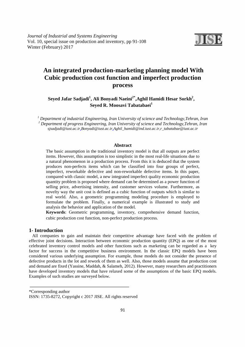
3-Problem definition Consider a manufacturer who produces a single product at a finite production rate N, and his production process due to natural phenomenon may produce non-perfect items. Hence, all items produced are screened, and inspection cost per item is included Cp. those Items that do not confirm to quality are withdrawn from the inventory and classify into various types of products –imperfect, defective but reworkable, and non-reworkable defective(see figure 2).The imperfect products are sold at the end of processing period as a single batch at a reduced price per unit that is a percentage of the selling price of good quality products, also, the rework process starts immediately after the regular production. The main objective of the present study is to maximize the total profit of the inventory system.

0

0.1

0.2

0.3

0.4

0.5

0.6

0.7

0.8

0.9

0.5069255660.4763268610.449436893

MC AC

Co

st

Output

0

50

100

150

200

250

300

350

400

450

Cp

Cost

Output

95

Fig. 2.Production system with rework

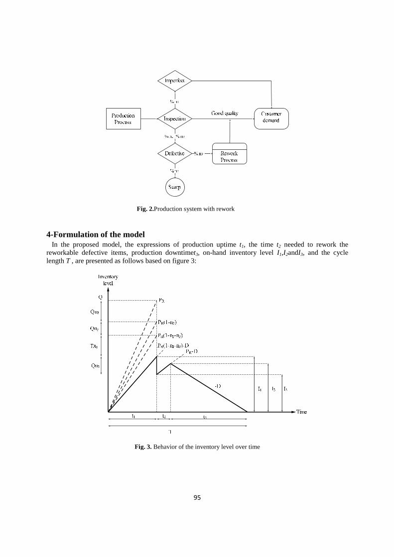
4-Formulation of the model In the proposed model, the expressions of production uptime t1, the time t2 needed to rework the reworkable defective items, production downtimet3, on-hand inventory level I1,I2andI3, and the cycle length T , are presented as follows based on figure 3:

Fig. 3. Behavior of the inventory level over time

96

(1) 3

1

,ii

T t=

=∑ (2) 1 31 ,r n n= − −

)3( 1 ,

R

Qt

P=

)4( 22 ,

R

n Qt

P=

)5( ,rQ

TD

=

)6( 1 2 30 1,n n n≤ + + ≤ The profit per cycle is determined as follows:

)7(

} } InventoryHolding CostReworking cost Interest/Depreciation CostSet-up CostSales Revenue Production Cost Maintenance Cos

1 2( ) ( ) ( , , ) ( )s R h Y s h Nprofit prQ ipn Q C AC Q AC c n Q C I C C C r C r= + − − − − − −6447448 64748 6447448 6447448 t

customer service costMarketing Cost

( ) ( )J L

j lj l

T M T S− × − ×∑ ∑

678

142431442443

Therefore, the per unit time profit function is given as:

j l 1 2 j l( , ( , , ) ( ) (1

, , , ) ( ) ( ))Ts s

J L

h Y s h Nl

Rj

Q C TR TC prQ ipnQ C AC Q AC cAP p C I C C C r C r T M Sn Q − − − ×

= − = + − − − −

+∑ ∑M S (8)

Note, the inventory holding cost in Eq. (8) is calculated as follows:

1 1 2 1 2

1 1 2

1 2 3

1 0

1( ) ( ) ( ) ( )

T t t t t t t

h h h h ht t t t t t t

I I IC I C q t dt C q t C q t C q t

T T

+ + +

= = = = +

+ + = = = + + ∫ ∫ ∫ ∫

In this model ( )q t is inventory level in time, so that, cab be rewritten

1 1 2 3 2 2 3

21 3 1 2 2 3

1 3

1 1 1 1( )

2 2 2

( (1 ) (1 2 (1 ) )).2 (1 )

h h h

hR

R

C I t C I I t C I tT

C QP n n D n n n n

P n n

= + + +

= − − − − + + −− −

(9)

Therefore, the joint production problem on base GP model for the problem can be written as,

( )

1 1 1 1 1j l 1 2

2

1 3 1 2 2 31 2

1 1 1 1Y

1 1

, , , )

(1 (1 2 (1 ) ))2 (1 )

( , , ) ( )

( , s s R

hR

R

J L

s h N J lj l

M Q C pD ipDn r C Dr Q CDr c CDn r

C QP n n D n n n n

P n n

C C C r Dr Q C r Dr

TP

S

a p

Q M

x − − − − −

− − − −

= =

= + − − −

− − − − − + + −− −

− − − −∑ ∑

M S

(10)

97

4- 1- The constraints There are some limitations to the maximizing Eq. (10) that cannot be ignored to derive the optimal total profit.

(i) Based on real world, the storage space for holding the inventory of all items is not unlimited. ,wrQ W≤

(ii) Investment amount on marketing and customer service cannot be infinite, it may have an upper limit on the maximum investment, i.e.,

J L

j l

( ) ,j lM S B+ ≤∑ ∑

(iii) An upper limit on the numbers of production cycles that can be made in a time cycle on the system, i.e.,

,D

LrQ

≤

(iv) The objective is to find out the optimal value such that total demand satisfied by the manufacturer should not be less than the minimum market share targeted,

MP Dψ ≤ (v) There is a limitation on the total resources available,

,bQ R≤

4- 2- Final Model By considering the previous section points’, and after substitutingD , pC , YC , hC and NC with

their corresponding equations, the EPQ can be rearranged as following optimization problem

j l 1

J L J L1 1 11

j l j l 2j=1 l=1 j=1 l=1

J L J L1 2 1

1 j l 2 2 j l 2j=1 l=1 j=1 l=1

J L1

3 j lj=1 l=1

, , , )

( ) (1 )

(1 ) (1

( ,

)

(1

j jl l

j jl l

j l

s R

R R

Q C

in kk p M S kC p M S r Q c n

r

ke p M S r Q c n ke p M S r Q c n

ke p M S r

Max TP p

β βτ τα α

β βτ τα α

β τα

− − − −

− − − −

− −

=

= + − − +

+ + − +

−

∏ ∏ ∏ ∏

∏ ∏ ∏ ∏

∏ ∏

M S

J L1 1 1

2 0 j lj=1 l=1

J L1 1 1 1 (1 )

1 2 2 3 j lj=1 l=1

J L J L J L1 1

j l j lj lj=1 l=1 j=1 l=1

) 0.5

(1 2 (1 ) )0.5

( )

.

j l

j l

j jl l

R

f fR s

l

c n ke p M S r Q drQ

n n n n kdP p M S r Q kd vC r Q

p M S kmr p M S Q M S

s t

bQ

β τα λ

β τα λ δ θ λ

β βτ γ τα α

− − − −

− − − − − − − − −

− −− − −

+ − +

− + + − −

− − +

≤

∏ ∏

∏ ∏

∑ ∑∏ ∏ ∏ ∏

J L

j l

1 1

J L1 1

j lj=1 l=1

,

( ) ,

,

,

,

l

j

j

l

j l

J L

M lj l

kp M S r

R

M S B

wrQ W

P kp M S

LQ

τ

β τα

βαψ

− −

= =

−

−

+ ≤

≤

≤

≤

∑ ∑

∏ ∏

∏ ∏

(11)

98

5- Modeling procedure The EPQ model formulated in the previous section is a constrained signomial GP with a degree difficulty 12, (DD=total number of terms -(total number of decision variable +1) (Duffin et al., 1967). In order to solve this model by GP modeling approach, it must betransformed to a standard form of GP. In the standard form of GP, the objective must be posynomial and it must be minimized, also, the inequality constraints can only have the form of a posynomial less than or equal to one(Boyd, Kim, Vandenberghe, & Hassibi, 2007). Due to this fact, in the rest of this section, a brief description of the method used to transform signomial GP to posynomial GP is proposed. Accordingly, although the EPQ model described in the previous section is not a standard GP, but it transformed to standard form in this section by using a trick. The trick mentioned in here refers to the concepts of the relations between geometric and arithmetic means (see equation 12).

11

( ) .n

N N

n n nnn

v vω ω==

≤∑∏ where1

1N

nn

ω=

=∑ (12)

In equation 12, denoted nv are positive numbers, and nω are nonnegative weights. Letting

. ,n i iv Uω ≡ so the inequality can be written as:

11

( ) n

N Nn

nnn n

UUω

ω ==

≤∑∏ (13)

Now, in order to use the above relations, the objective function of the EPQ model can be expressed as follows.

1 1 2( , , , , , )j lMaxTP p C r Q U U= −M S (14)

Here, if in order to simplify the objective function, considering following notations

11 ( ),

iF

n kk

r+= , (15)

22 (1 ),Rc nF += (16) 1 23 2 3(1 2 (1 ) ),nF n n n− + + −= , (17)

The parameters U1 and U2 can be defined as follows

99

j

J L J L1 1 1

1 j 2 2 j l 3j=1 l=1 j=1 l=1

J L1 1

j lj=1 l=1

J L J L1 1 1 2

2 j l 2 1 j l 2 3j=1 l=1 j=1 l=1

J1

j lj 1

1

2=

0.5jl l

j l

j jl l

j l

l

s

F p M S F ke p M S r Q F kdP p

M S r Q

U kC p M S r Q F ke p M S r Q F ke p

M S r F k

U β βτ τα α α

β τ λ

β βτ τα α α

β τ

− − − − −

− −

− − − − − −

−

=

+ +

+ +

+

=

∏ ∏ ∏ ∏

∏ ∏

∏ ∏ ∏ ∏

∏L J L

1 1 10 j l

l=1 j=1 l=1

J L J L J L1 1 1

l j l j lj lj=1 l=1 j=1 l=1

0.5

( ) ( )

j l

j jl l

fs

f

e p M S r Q rQ kd vC p

M S r Q kmr p M S Q M S

β τα λ δ α

β βτ τθ λ γ α

− − − − − − −

− − − − − −

+ +

+ + +

∏ ∏ ∏

∑ ∑∏ ∏ ∏ ∏

(18)

Then, there the objective function, by definition one auxiliary variable and constraint can be written as

j l 1

1 2

( , , , , )

,

Q C Z

U

Max T

U

p

Z

P =

− ≥

M S

The constraint cab be transformed to two constraints following by definition a new X variable, 1 1

21 2 1 2 1 2 1

1

1, (1)

1, (2)

ZX U XU U Z U Z U U X Z U

U X

− −

−

+ ≤− ≥ ⇒ ≥ + ⇒ ≥ ≥ + ⇒ ≥

(19)

(20)

The model above is a non-standard Posynomial GP, in order to transform this model to standard GP form ( 1≤ ), here the reversed GP approach is applied (Beightler & Phillips, 1976; Chiang, 2005). Base on the approach, Eq. (13) hold at equalities if and only if:

1

nn N

nn

U

Uω

=

=∑

where 0ω > (21)

As,a lower bound inequality on the posynomialnU can be approximated by an upper bound inequality on the following monomial:

1

1 1 11 1

1

( ) 1 ( ) 1 ( ) 1n n

N NN N Nif asn n n

n n n nNn n nn nn n

nn

U U UU U U

U

ω ωωω ω

−−

= = == =

=

≤ → = → ≥ ⇒ ≤ ⇒ ≤∑ ∑ ∑∏ ∏∑

(22)

Therefore, in the proposed model, for the second constraint, we have:

3 31 1

1 1 1 11 1

1 1,asn n

n n

U U U X U X− −

= =

= → ≥ ⇒ ≥∑ ∑

31 231 1 1311 12

11 1 2 3

( ) 1 1,asn

n

UU UU X

ωω ω

ω ω ω

−− −− −

=

≤ → ≤

∑

(23)

Also, from equation (21), we obtain:

11

1 1

1 1 1 1 11 2 2 3

1 1 1

1

1 1 1

0.,

5j

j l

j jl l l

J L

j lj l

J L J L J L

j l j l j lj l j l j l

F p M S

F p M S F ke p M S r Q F kdP p M S r Q

β τα

β β βτ τ τα α α λω

−

= =

− − − − − − −

= = = = = =

+ +=

∏ ∏

∏ ∏ ∏ ∏ ∏ ∏ (24)

100

12 2

1 1

1 1 1 1 11 2 2 3

1 1 1 1 1

2

1

0.5,

j

j l

j jl l l

J L

j lj l

J L J L J L

j l j l j lj l j l j l

F ke p M S r Q

F p M S F ke p M S r Q F kdP p M S r Q

β τα

β β βτ τ τα α α λω

− −

= =

− − − − − − −

= = = = = =

+ +=

∏ ∏

∏ ∏ ∏ ∏ ∏ ∏

1 1 13

1 1

1 1 1 1 11 2 2 3

1 1 1 1 1 1

3

0.5

0.5,

j

j l

j jl l l

J L

j lj l

J L J L J L

j l j l j lj l j l j l

F kdP p M S r Q

F p M S F ke p M S r Q F kdP p M S r Q

β τα λ

β β βτ τ τα α α λω

− − − −

= =

− − − − − − −

= = = = = =

+=

+

∏ ∏

∏ ∏ ∏ ∏ ∏ ∏

And for the first constraint, we have:

9 91 1 1 1

2 2 2 21 1

1 1,asn n

n n

U U ZX U X ZX U X− − − −

= =

= → + ≤ ⇒ + ≤∑ ∑ (25)

Finally, after rearranging primary constraints, the EPQ model can be rewritten as follows:

1 2

3

1j l 1

1 1 1 11 2 2

1 1 1 1

1 1 1 13

1 1

1

1 2

3

( , , , , ) ( )

0.5

.

1,

j jl l

j l

J L J L

j l j lj l j l

J L

j lj l

s

Q C Z Z

F p M S X F ke p M S r QX

F kdP p M S r Q X

Z

MinTP p Max

X kC p M

s t

β βτ τα α

β τα λ

α

ω ω

ω

ω ω

ω

−

− − − − −

= = = =

− − − − −

= =

−

− −

−

−

≤

= =

+

∏ ∏ ∏ ∏

∏ ∏

M S

J L J L1 1 1 1 2 1

j l 2 1 j lj=1 l=1 j=1 l=1

J L J L1 1 1 1 1

2 3 j l 2 0 j lj=1 l=1 j=1 l=1

J L1 1 1 1 1

j lj=1 l=1

j

0.5

j jl l

j jl l

j l

j

f fs

S r Q X F ke p M S r Q X

F ke p M S r X F ke p M S r Q X

rQ X kd vC p M S r Q X kmr p

M S

β βτ τα

β βτ τα α

β τλ δ α θ λ γ α

β

− − − − − −

− − − − − − −

− − − − − − − − − − −

+

+ +

+ + +

∏ ∏ ∏ ∏

∏ ∏ ∏ ∏

∏ ∏J L J L

1 1 1 1l j l

j lj=1 l=1

J L1 1

j lj=1 l

1

J L1

j

1

1

=

l

1

1

1

1

(

1,

( ) 1,

1,

) ( ) 1,

1,

1,

l

j l

j l

j l

J L

M lj l

bQR

M S B

wr

Q X M

QW

P k p M S

X S X

kp M S r Q L

β τ

τ

β τα

αψ

−

−

−

− −−

=

− − − −

− − −−

=

+ + ≤

≤

+ ≤

≤

≤

≤

∑ ∑

∑

∏ ∏

∏

∑

∏ ∏

∏

(26)

101

6- Solution approach and numerical experiment To illustrate the validity of the proposed model and the usefulness of the proposed solution method, a simple numerical experiment is presented and the related results are reported in this section. To this end, consider a company who wants to sell its commodity regarding two methods for advertising (TV, Newspaper) as well as providing two types service to consumers (Buying advice, Product Warranty).The other required information to decision-making is set from marketing and production departments as follows:

1 0.12,τ = 2 0.11,β = 1 0.13,β = 2.55,α = 3 10 ^13,k = ×

0 141,e = 3 63.48,e = 2 12.96,e = 1 0.94,e = 2 0.1,τ =

0.15,d = 0.2,λ = 334,L = 0.1,f = 0.70,i = 5,v = 4700000,B =

0.19,ψ = 0.34,Rc = 4110 ,0MP ×=

5,b = 10,m = 0.5,γ = 4,θ = 3.5,δ =

1 0.23,n = 10000,P = 1900,W = 23,w = 1000,R =

3 0.03,n = 2 0.01,n =

The EPQ model (26) is a very complex GP problem. so, unlike conventional method in the literature(Duffin et al., 1967).this paper uses the latest software development for determining the optimal closed form solution. The results of running the CVX for optimum conditions (*) are as follows:

* $656,526,287Z = * 90Q = * 47$ ,460p = *1 1,305 62$ ,7M =

*2 1,104 21$ ,4M =

*1 1,249 34$ ,0S = *

2 1,040 87$ ,5S = * $1.63SC =

In addition, total demand achieved by the manufacturer, which is a power function of decision variables, is * 22,160D = .

6- 1- Sensitive analysis To analyze the effects of main parameters changes on the optimal solution, a sensitivity analysis is performed on the examples described in the previous section. First, we have to admit a fact that due to high degrees of nonlinearities of the model it is not always possible to expect a certain behavior of the decision variables. However, figures (4)-(18) show the results of sensitive analysis on the main parameters. The following conclusions can be drawn from figures (4) - (18):

� *Z is highly sensitive to the changes in parameterα (figure 4).This is because with the decline in theα , ( 2.55 ( 0.01)H H= − × ), it can be concluded that sensitive price of customers to the commodity is reduced, and as a result, the company can raise its commodity price without any threat (figure 5). Also, asα decreases, due to restriction on the investment on the various methods of marketing and types of customers’ service, the company directs funds toward effective options of marketing methods and customer service types (figure 6).Finally, as α decreases, from figure 7, it can be seen that the lot-size has a reverse relationship withα . This is because that the company is not limited to the inventory holding costs and production cost due to increased revenue.

� *Z is highly sensitive to the changes in parametersjβ and lτ ( j and 1,2l = )

102

( 0 0( ) ( ) ( 0.017)j l j l Hβ τ β τ= + × ) where and another equations0 jβ and 0lτ refers to the default

example values. Generally, when customers get more sensitive to the marketing and customer service there is an incentive for the company to increases its investment in the marketing and customer service. From the results of analyses (figure 8), we can see when jβ and lτ increased

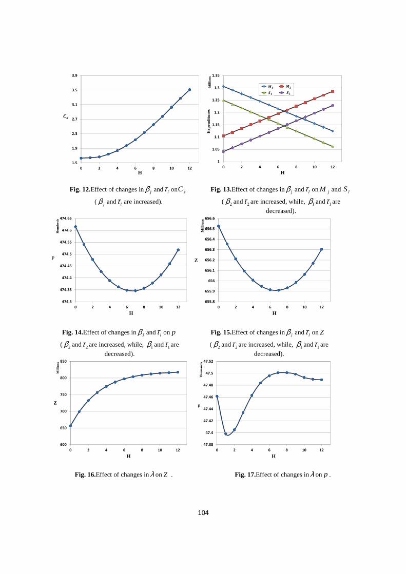
simultaneously by a similar amount, the company in order to maximize total profit should allocate limited budget to various options of marketing and customer service. As a result of this allocation, the company will be able to raise its commodity price (figure 9) and, subsequently, its profit increases (figure 10), so that it does not feel any pressure against the increased cost of inventory holding and production, due to increasing the lotsize, and increase in setup cost (see figures 11 and 12).

� Base on the figure 8, we reached to this conclusion that the company should allocate limited budget to various options of marketing and customer service. Nevertheless, according to figures. 13-15, this investment should be in a diverse range of options of marketing and customer service with different elasticity values. So that it is seen that when values of 2β and 2τ are increased

according to the equation2 2 0 0( ) ( ) ( 0.0015)j l Hβ τ β τ= + × , while simultaneously, 1β and 1τ are

decreased according to1 1 0 0( ) ( ) ( 0.0015)j l Hβ τ β τ= − × , *2M and *

2S increase, and both *1M

and *1S decrease (figure 13). Also, figures 14 and 15 show when jβ and lτ get closer to each

other, the commodity price, and total annual profit decrease.

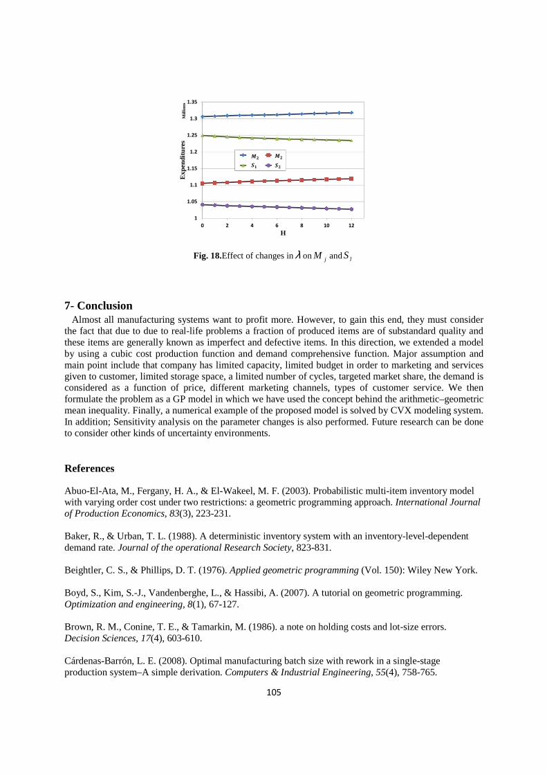
� According to figures 16 and 17, *p and *Z are moderately sensitive to the changes in the

parameterλ . So that when λ increases ( 0.2 ( 0.08)Hλ = + × ), then *p and *Z increase; and

when rate increases of *Z decreases, the company the company directs funds toward effective options of marketing methods and customer service types (where it is assumed that1β and lτ are

constant)(see figure 18).

Fig.4. Effect of changes inα onZ Fig. 5.Effect of changes inα on p

550

650

750

850

950

1050

1150

1250

1350

1450

0 2 4 6 8 10 12

Z

Mill

ions

H

40

45

50

55

60

65

70

75

80

0 2 4 6 8 10 12

P

Tho

usan

ds

H

103

Fig. 6.Effect of changes inα onQ Fig. 7.Effect of changes inα on jM and lS

Fig. 8.Effect of changes in jβ and lτ on Z

( jβ and lτ are increased).

Fig. 9.Effect of changes in jβ and lτ on p

( jβ and lτ are increased).

Fig. 10.Effect of changes in jβ and lτ onQ

( jβ and lτ are increased).

Fig. 11.Effect of changes in jβ and lτ on jM

and lS ( jβ and lτ are increased).

85

90

95

100

105

110

115

0 2 4 6 8 10 12

Q

H

1

1.05

1.1

1.15

1.2

1.25

1.3

1.35

0 2 4 6 8 10 12

Exp

endi

ture

sM

illio

ns

H

. .

. .��

��

��

��

0

2E+10

4E+10

6E+10

8E+10

1E+11

1.2E+11

0 2 4 6 8 10 12

Z

H

0

500

1000

1500

2000

2500

3000

3500

4000

4500

0 2 4 6 8 10 12

P

Tho

usan

ds

H

80

85

90

95

100

105

110

115

0 2 4 6 8 10 12

Q

H

1.02

1.07

1.12

1.17

1.22

1.27

1.32

0 2 4 6 8 10 12

Exp

endi

ture

sM

illio

ns

H

. .

. .

�� ��

�� ��

104

Fig. 12.Effect of changes in jβ and lτ on sC

( jβ and lτ are increased).

Fig. 13.Effect of changes in jβ and lτ on jM and lS

( 2β and 2τ are increased, while, 1β and 1τ are

decreased).

Fig. 14.Effect of changes in jβ and lτ on p

( 2β and 2τ are increased, while, 1β and 1τ are

decreased).

Fig. 15.Effect of changes in jβ and lτ onZ

( 2β and 2τ are increased, while, 1β and 1τ are

decreased).

Fig. 16.Effect of changes inλ onZ . Fig. 17.Effect of changes inλ on p .

1.5

1.9

2.3

2.7

3.1

3.5

3.9

0 2 4 6 8 10 12

.

H

��

1

1.05

1.1

1.15

1.2

1.25

1.3

1.35

0 2 4 6 8 10 12

Exp

endi

ture

sM

illio

ns

H

. .

. .

��

��

��

��

474.3

474.35

474.4

474.45

474.5

474.55

474.6

474.65

0 2 4 6 8 10 12

P

Hun

dred

s

H

655.8

655.9

656

656.1

656.2

656.3

656.4

656.5

656.6

0 2 4 6 8 10 12

Z

Mill

ions

H

600

650

700

750

800

850

0 2 4 6 8 10 12

Z

Mill

ions

H

47.38

47.4

47.42

47.44

47.46

47.48

47.5

47.52

0 2 4 6 8 10 12

p

Tho

usan

ds

H

105

Fig. 18.Effect of changes inλ on jM and lS

7- Conclusion Almost all manufacturing systems want to profit more. However, to gain this end, they must consider the fact that due to due to real-life problems a fraction of produced items are of substandard quality and these items are generally known as imperfect and defective items. In this direction, we extended a model by using a cubic cost production function and demand comprehensive function. Major assumption and main point include that company has limited capacity, limited budget in order to marketing and services given to customer, limited storage space, a limited number of cycles, targeted market share, the demand is considered as a function of price, different marketing channels, types of customer service. We then formulate the problem as a GP model in which we have used the concept behind the arithmetic–geometric mean inequality. Finally, a numerical example of the proposed model is solved by CVX modeling system. In addition; Sensitivity analysis on the parameter changes is also performed. Future research can be done to consider other kinds of uncertainty environments.

References

Abuo-El-Ata, M., Fergany, H. A., & El-Wakeel, M. F. (2003). Probabilistic multi-item inventory model with varying order cost under two restrictions: a geometric programming approach. International Journal of Production Economics, 83(3), 223-231. Baker, R., & Urban, T. L. (1988). A deterministic inventory system with an inventory-level-dependent demand rate. Journal of the operational Research Society, 823-831. Beightler, C. S., & Phillips, D. T. (1976). Applied geometric programming (Vol. 150): Wiley New York. Boyd, S., Kim, S.-J., Vandenberghe, L., & Hassibi, A. (2007). A tutorial on geometric programming. Optimization and engineering, 8(1), 67-127. Brown, R. M., Conine, T. E., & Tamarkin, M. (1986). a note on holding costs and lot-size errors. Decision Sciences, 17(4), 603-610. Cárdenas-Barrón, L. E. (2008). Optimal manufacturing batch size with rework in a single-stage production system–A simple derivation. Computers & Industrial Engineering, 55(4), 758-765.

1

1.05

1.1

1.15

1.2

1.25

1.3

1.35

0 2 4 6 8 10 12

Exp

endi

ture

sM

illio

ns

H

. .

. .��

��

�� ��

106

Chan, W., Ibrahim, R., & Lochert, P. (2003). A new EPQ model: integrating lower pricing, rework and reject situations. Production Planning & Control, 14(7), 588-595. Chen, C.-K. (2000). Optimal determination of quality level, selling quantity and purchasing price for intermediate firms. Production Planning & Control, 11(7), 706-712. Cheng, T. (1989). An economic order quantity model with demand-dependent unit cost. European Journal of Operational Research, 40(2), 252-256. Chiang, M. (2005). Geometric programming for communication systems: Now Publishers Inc. Duffin, R. J., Peterson, E. L., & Zener, C. (1967). Geometric programming: theory and application: Wiley New York. F. Ghazi Nezami , S. J. S., Mir B. Aryanezhad. (2009). A Geometric Programming Approach for a Nonlinear Joint Production- Marketing Problem. International Association of Computer Science and Information Technology - Spring Conference . Fathian, M., Sadjadi, S. J., & Sajadi, S. (2009). Optimal pricing model for electronic products. Computers & Industrial Engineering, 56(1), 255-259. Groenevelt, H., Pintelon, L., & Seidmann, A. (1992). Production lot sizing with machine breakdowns. Management Science, 38(1), 104-123. Gujarati, D. N. (2003). Basic Econometrics. 4th: New York: McGraw-Hill. Hayek, P. A., & Salameh, M. K. (2001). Production lot sizing with the reworking of imperfect quality items produced. Production Planning & Control, 12(6), 584-590. Islam, S. (2008). Multi-objective marketing planning inventory model: A geometric programming approach. Applied Mathematics and Computation, 205(1), 238-246. Jamal, A., Sarker, B. R., & Mondal, S. (2004). Optimal manufacturing batch size with rework process at a single-stage production system. Computers & Industrial Engineering, 47(1), 77-89. Jung, H., & Klein, C. M. (2001). Optimal inventory policies under decreasing cost functions via geometric programming. European Journal of Operational Research, 132(3), 628-642. Jung, H., & Klein, C. M. (2006). Optimal inventory policies for profit maximizing EOQ models under various cost functions. European Journal of Operational Research, 174(2), 689-705. Khanra, S., & Chaudhuri, K. (2003). A note on an order-level inventory model for a deteriorating item with time-dependent quadratic demand. Computers & operations research, 30(12), 1901-1916. Kim, D., & Lee, W. J. (1998). Optimal joint pricing and lot sizing with fixed and variable capacity. European Journal of Operational Research, 109(1), 212-227. Kotb, K. A., & Fergany, H. A. (2011). Multi-item EOQ model with both demand-dependent unit cost and varying leading time via geometric programming. Applied Mathematics, 2(5), 551-555.

107

Lee, J. S., & Park, K. S. (1991). Joint determination of production cycle and inspection intervals in a deteriorating production system. Journal of the operational Research Society, 775-783. Lee, W. J. (1993a). Determining Order Quantity and Selling Price by Geometric Programming: Optimal Solution, Bounds, and Sensitivity. Decision Sciences, 24(1), 76-87. Lee, W. J. (1993b). Optimal order quantities and prices with storage space and inventory investment limitations. Computers & Industrial Engineering, 26(3), 481-488. Lee, W. J., & Kim, D. (1993). Optimal and heuristic decision strategies for integrated production and marketing planning. Decision Sciences, 24(6), 1203-1214. Lin, C.-S. (1999). Integrated production-inventory models with imperfect production processes and a limited capacity for raw materials. Mathematical and Computer Modelling, 29(2), 81-89. Liu, J. J., & Yang, P. (1996). Optimal lot-sizing in an imperfect production system with homogeneous reworkable jobs. European Journal of Operational Research, 91(3), 517-527. Mandal, N. K., Roy, T. K., & Maiti, M. (2006). Inventory model of deteriorated items with a constraint: a geometric programming approach. European Journal of Operational Research, 173(1), 199-210. Panda, D., & Maiti, M. (2009). Multi-item inventory models with price dependent demand under flexibility and reliability consideration and imprecise space constraint: A geometric programming approach. Mathematical and Computer Modelling, 49(9), 1733-1749. Rosenblatt, M. J., & Lee, H. L. (1986). Economic production cycles with imperfect production processes. IIE transactions, 18(1), 48-55. Sadjadi, S. J., Aryanezhad, M.-B., & Jabbarzadeh, A. (2009). An integrated pricing and lot sizing model with reliability consideration. Paper presented at the Computers & Industrial Engineering, 2009. CIE 2009. International Conference on. Sadjadi, S. J., Oroujee, M., & Aryanezhad, M. B. (2005). Optimal production and marketing planning. Computational Optimization and Applications, 30(2), 195-203. Salameh, M., & Jaber, M. (2000). Economic production quantity model for items with imperfect quality. International Journal of Production Economics, 64(1), 59-64. Sana, S., Goyal, S., & Chaudhuri, K. (2004). A production–inventory model for a deteriorating item with trended demand and shortages. European Journal of Operational Research, 157(2), 357-371. Sana, S. S., & Chaudhuri, K. (2008). A deterministic EOQ model with delays in payments and price-discount offers. European Journal of Operational Research, 184(2), 509-533. Subramanyam, E. S., & Kumaraswamy, S. (1981). EOQ formula under varying marketing policies and conditions. AIIE Transactions, 13(4), 312-314. Yassine, A., Maddah, B., & Salameh, M. (2012). Disaggregation and consolidation of imperfect quality shipments in an extended EPQ model. International Journal of Production Economics, 135(1), 345-352.

108

You, P.-S. (2005). Inventory policy for products with price and time-dependent demands. Journal of the Operational Research Society, 56(7), 870-873. You, P.-S., & Hsieh, Y.-C. (2007). An EOQ model with stock and price sensitive demand. Mathematical and Computer Modelling, 45(7), 933-942. Yum, B. J., & Mcdowellj, E. d. (1987). Optimal inspection policies in a serial production system including scrap rework and repair: an MILP approach. International Journal of Production Research, 25(10), 1451-1464.