lable at ScienceDirect

Renewable Energy 71 (2014) 553e562

Contents lists avai

Renewable Energy

journal homepage: www.elsevier .com/locate/renene

An integrated reservoir-power system model for evaluating theimpacts of wind integration on hydropower resources*

Jordan D. Kern a, *, Dalia Patino-Echeverri b, Gregory W. Characklis a

a University of North Carolina at Chapel Hill, Department of Environmental Sciences and Engineering, Rosenau Hall CB #7431, Chapel Hill, NC 27599-7431,United Statesb Duke University, Nicholas School of the Environment A150 LSRC, Box 90328, Durham, NC 27708, United States

a r t i c l e i n f o

Article history:Received 22 October 2013Accepted 10 June 2014Available online 28 June 2014

Keywords:Wind energyHydropowerPower system analysisDam operationsUnit commitmentRiver flows

* This work was funded by the Hydropower ReseaDepartment of Energy, Wind and Water Power Techn* Corresponding author. Tel.: þ1 2023650095.

E-mail addresses: jdkern@live.unc.edu (J.D. K(D. Patino-Echeverri), charack@email.unc.edu (G.W. C

http://dx.doi.org/10.1016/j.renene.2014.06.0140960-1481/© 2014 Elsevier Ltd. All rights reserved.

a b s t r a c t

Despite the potential for hydroelectric dams to help address challenges related to the variability andunpredictability of wind energy, at present there are few systems-based wind-hydro studies available inthe scientific literature. This work represents an attempt to begin filling this gap through the develop-ment of a systems-based modeling framework for analysis of wind power integration and its impacts onhydropower resources. The model, which relies entirely on publicly available information, was developedto assess the effects of wind energy on hydroelectric dams in a power system typical of the SoutheasternUS (i.e., one in which hydropower makes up <10% of total system capacity). However, the model caneasily reflect different power mixes; it can also be used to simulate reservoir releases at self-scheduled(profit maximizing) dams or ones operated in coordination with other generators to minimize totalsystem costs. The modeling framework offers flexibility in setting: the level and geographical distributionof installed wind power capacity; reservoir management rules, and static or dynamic fuel prices forpower plants. In addition, the model also includes an hourly ‘natural’ flow component designedexpressly for the purpose of assessing changes in hourly river flow patterns that may occur as aconsequence of wind power integration. Validation of the model shows it can accurately reproducemarket price dynamics and dam storage and release patterns under current conditions. We alsodemonstrate the model's capability in assessing the impact of increased wind market penetration on thevolumes of reserves and electricity sold by a hydroelectric dam.

© 2014 Elsevier Ltd. All rights reserved.

1. Introduction

The extent to which large scale integration of wind energy inelectric power systems will impact market prices, system costs andreliability may depend greatly on the availability of sources that canquickly change (or ‘ramp’) electricity output [1e3]. Due to theircapacity for energy storage, lowmarginal costs, and fast ramp rates,hydroelectric dams are often regarded as an ideal resource formitigating problematic issues related to wind's intermittency andunpredictability [4]. In recent years, researchers have investigated awide range of topics concerning the coordinated use of wind andhydropower. However, few studies to date have made use of

rch Foundation and the U.S.ologies program.

ern), dalia.patino@duke.eduharacklis).

comprehensive reservoir and power system models in assessingthe costs and benefits of wind-hydro projects, and the developmentof such models remains a limiting factor in addressing a number ofunanswered questions in this area.

Previous studies of wind-hydro projects can be separatedconceptually into two categories of analysis: ‘pairwise’ and ‘sys-tem-based’ [4]. Pairwise analyses evaluate the costs and benefits ofwind-hydro projects operated in isolation (i.e., somewhat discon-nected from other elements of a larger electric power system).Simpler examples include investigations of the capacity value [5]and firm energy costs [6,7] of wind-hydro projects. More sophis-ticated pairwise studies have used historical market prices torepresent wind-hydro projects' connection to larger electric powersystems. Examples include previous research on: the value of en-ergy storage in wind-hydro systems [8,9]; the financial and envi-ronmental costs of dams' providing a ‘wind firming’ service [10];project optimization [11]; the use of dams to increase wind marketpenetration [12]; and the use of multipurpose dams to integratewind energy [13]. Pairwise wind-hydro studies, particularly those

J.D. Kern et al. / Renewable Energy 71 (2014) 553e562554

that include some consideration of a project's system context, canoffer valuable insights. However, they are generally less capable ofcapturing the more complex, endogenous economic and opera-tional consequences of large scale wind integration for generatorsand consumers [4].

More comprehensive ‘system-based’ models simulate the effectof wind power integration on the workings of entire electric powersystems made up of many different sizes and types of generators. Assuch, they offer the significant advantage of being able to simulatechanges in market prices and system costs that may occur as a resultof wind power integration, and then evaluate how these changescould impact the use of hydroelectric dams. However, most previoussystem-based wind-hydro studies have been conducted by electricpower utilities, and detailed modeling information (and even re-sults) from these studies is generally considered proprietary [4].Examples of system-based studies from academic literature includeinvestigations of the impacts of wind-hydro projects on: the value ofwind energy [14]; and the cost of reducing CO2 emissions [15].

Few wind-hydro studies to date have taken a system-basedapproach. As a consequence, significant gaps in knowledgeremain as to how wind power integration may impact hydropowerresources. For example: in all but a few US states, hydropowermeets less than 10% of total annual electricity demand; but most (ifnot all) system-based wind-hydro studies have focused on ‘hydrodominant’ systems, in which hydropower makes up a much largerpercentage of total system generation. The effects of wind powerintegration on dam operations may be much different in a systemwith relatively little hydropower capacity. There has likewise beenlittle consideration in previous studies given to the role of markettype (i.e., regulated versus competitive) in framing the incentivestructure for hydroelectric dams to help integrate intermittentwind energy. In addition, no system-based study has addressed thepotential for wind energy to impact environmental flows down-stream of hydroelectric dams. Investigation of these topics requiresmodels that can simulate the effects of wind power integration onhydroelectric dams under a variety of structural, economic, andhydrological conditions, while also maintaining the operationalcomplexity of interconnected reservoir and electric power systems.

At present, there are few systems-based wind-hydro studiesavailable in the scientific literature. This work represents an attemptto begin filling this gap through the development of a systems-based modeling framework for analysis of wind power integrationand its impacts on hydropower resources. The model, which reliesentirely on publically available information, was developed toassess the effects of wind energy on hydroelectric dams in a powersystem typical of the Southeastern US (i.e., one in which hydro-power makes up <10% of total system capacity). However, themodel can easily reflect different powermixes; it can also be used tosimulate reservoir releases at self-scheduled (profit maximizing)dams or ones operated in coordination with other generators tominimize total system costs. The modeling framework offers flexi-bility in setting: the level and geographical distribution of installedwind power capacity; reservoir management rules, and static ordynamic fuel prices for power plants. In addition, the model alsoincludes an hourly ‘natural’ flow component designed expressly forthe purpose of assessing changes in hourly flow patterns that mayoccur as a consequence of wind power integration.

2. Methods

The reservoir-power system model consists of: 1) an electricitymarket (EM) model; and 2) a reservoir system model. The EMmodel iteratively solves two linked mixed integer optimizationprograms, a unit commitment and economic dispatch problem, toallow a power system operator to meet fluctuating hourly

electricity demand. A single iteration of the EM model and its twosub problems yields hourly market prices for a single 24 h period.

The reservoir system model consists of: 1) an hourly naturalflowmodel that simulates ‘natural’ (pre-dam) flows at dam sites; 2)a daily reservoir operations model that determines availablereservoir storage for hydropower production; and 3) a hydropowerdispatch model that schedules hourly reservoir releases in order tomaximize dam profits. Fig. 1 shows a schematic of the integratedreservoir (components shown in dark grey) and EM (componentsshown in light grey) model.

2.1. Electricity market model

The EMmodel was developed in order to simulate the operationof a large power system based on the Dominion Zone of PJMInterconnection (a wholesale electricity market located in the Mid-Atlantic region of the U.S). Dominion's total generation capacity isapproximately 23 GW, with a peak annual electricity demand ofroughly 19 GW. Using the Environmental Protection Agency's (EPA)2010 eGrid database, each generator in the utility's footprint wascataloged by generating capacity (MW), age, fuel type, primemoverand average heat rate (MMBtu/MWh). Specific operating con-straints parameters were estimated for each size and type of plantusing industry, governmental and academic sources. To reduce thecomputational complexity of the EM model (i.e., maintain reason-able solution times) units from each plant type were clustered byfixed and variable costs of electricity and reserves, with each clusterof similar generators forming a ‘composite’ plant. The total numberof power plants represented in the model was reduced from 68 to amore manageable, yet representative, quantity (24)dwith totalsystem wide capacity remaining the same. Each generator in themodeled system belongs to one of eight different power planttypes: conventional hydropower, pumped storage hydropower,coal, combined cycle natural gas (NGCC), combustion turbine nat-ural gas (NGCT), oil, nuclear or biomass. Table 2 of supplementalmaterials section shows detailed operating characteristics of eachplant in the modeled generation portfolio.

The EM model has two main components: 1) a unit commit-ment (UC) problem that represents both ‘day ahead’ electricity and‘reserves’markets; and 2) an economic dispatch (ED) problem thatrepresents a ‘real time’ electricity market [16].

2.1.1. Unit commitment problemThe UC problem uses information regarding the costs (variable,

fixed, and start) of participating power plants to schedule the status(on/off) and generation (MWh) at each plant in the system 24 h inadvance. The UC problem is responsible for meeting forecast ‘dayahead’ (DA) electricity demand and satisfying system wide re-quirements for the provision of spinning and non spinning ‘re-serves’ (unscheduled generating capacity that is set aside for thenext day as ‘back up’). The objective function of the UC problem isto minimize the cost of meeting forecast electricity demand andreserve requirements over a 96 h planning horizon, given a diversegeneration portfolio:

Minimize ZUCX96

t¼1

XJ

j

��DA MWht;j*VCj

�þ �ONt;j*FCj

�

þ ðSRV MWt;j*VC SRjÞ þ ðSRV ONt;j*FC SRjÞþ ðNRV MWt;j*VC NRjÞ þ

�STARTt;j*SCj

��

(1)

where, t ¼ hour in planning horizon 2{1,2,…96}, j ¼ generator insystem portfolio.

Fig. 1. Conceptual framework of integrated reservoir-power system model. Orange boxes denote computing order; light grey boxes denote components of the electricity market(EM) model; and dark grey boxes denote components of the reservoir system model. (For interpretation of the references to colour in this figure legend, the reader is referred to theweb version of this article.)

J.D. Kern et al. / Renewable Energy 71 (2014) 553e562 555

Decision variables

� DA_MWht,j ¼ DA electricity scheduled in hour t at generator j(MWh).

� ONt,j ¼ Binary ‘on/off’ variable indicating DA electricityproduction.

� SRV_MWt,j ¼ Spinning reserve capacity scheduled in hour t atgenerator j (MW).SRV_ONt,j ¼ Binary ‘on/off’ variable indicating spinning reserveprovision.

� NRV_MWt;j ¼Non spinning reserve capacity scheduled in hour tat generator j (MW).

� STARTt,j ¼ Binary ‘on/off’ variable indicating plant start.

Parameters

� VCj ¼ Variable cost of DA electricity production at generator j($/MWh).

� FCj ¼ Fixed cost of DA electricity production at generator j ($).� VC_SRj ¼ Variable cost of spinning reserve at generator j($/MWh).

� FC_SRj ¼ Fixed cost of spinning reserve provision at generator j($).

� VC_NRj ¼ Variable cost of non spinning reserve at generator j($/MW).

� SCj ¼ Start cost of generator j.

Solution of the UC problem yields a preliminary hourlyschedule of DA electricity generation and provision of reserves foreach plant in the system over the entire planning horizon(t ¼ 1,2,…96). However, only the first 24 h of the calculatedoperating schedule is considered ‘locked in’dscheduled genera-tion and reserves for later hours, i.e., t ¼ 25, 26,… 96, are

immediately discarded. This strategy ensures that plant operatingschedules are conditioned on multi-day forecast information forelectricity demand, wind availability, and hydropower capacity,but it also makes sure plant operations are formally scheduled nomore than 24 h in advance. Market prices for both DA electricityand reserves for hours t ¼ 1,2,…24 are then determined by thevariable cost of the most expensive plant used to meet demand ineach market, respectively.

2.1.2. Economic dispatch problemAfter the UC problem is solved, the model adjusts in real time

via the economic dispatch (ED) problem. The ED problem repre-sents the operation of a ‘real time’ (RT) electricity market thatcompensates for demand forecast error, forced reductions in po-wer plant output, and/or wind forecast errors by schedulinggeneration from system reserves. The objective function for the EDproblem is to minimize the cost of meeting RT electricity demandover a 24 h planning horizon (t ¼ 1,2,…24) using generation ca-pacity that was designated one day prior as reserves by the UCproblem:

Minimize ZED :X24

t¼1

XPp

�RT MWht;p*VCp

�

þX24

t¼1

XNn

�ðRT MWht;n*VCnÞ þ ðRT ONt;n*FCnÞ

þ �STARTt;n*SCn

��

(2)

where, t ¼ hour in planning horizon 2{1,2,…24}.p ¼ generator in spinning reserves portfolio n ¼ generator in

non spinning reserves portfolio.

J.D. Kern et al. / Renewable Energy 71 (2014) 553e562556

Decision variables

� RT_MWht,p ¼ RT electricity produced in hour t using spinningreserves from generator s (MWh).

� RT_MWht,n ¼ RT electricity produced in hour t using non spin-ning reserves from generator n (MWh).

� RT_ONt,n ¼ Binary ‘on/off’ variable indicating real time elec-tricity production from non spinning reserves at generator n.

� STARTt,n ¼ Binary ‘on/off’ variable indicating plant start (Non-spinning generator).

Parameters

� VCp ¼ Variable cost of RT electricity production at generator p($/MWh).

� VCn ¼ Variable cost of RT electricity production at generator n($/MWh).

� FCn ¼ Fixed cost of electricity production at generator n ($).� SCn ¼ Start cost of generator n.

Solution of the ED problem yields an hourly schedule of RTelectricity generation from each plant in the system's combinedspinning and non-spinning reserves portfolio over the planninghorizon (t ¼ 1,2,…24). RT electricity prices are then set by thevariable cost of the most expensive generator used tomeet demandin each hour. After the ED problem is solved, the larger electricitymarket (EM) model shifts 24 h into the future and begins its twostage process again.

Both the UC and ED problems are subject to a number of con-straints, which can be separated conceptually into two classes: 1)constraints that enforce adherence to plant specific operatingcharacteristics (e.g., minimum/maximum generating capacities,maximum ramp rates, minimum up/down times, etc.); and 2)constraints that apply to overall system operation (e.g., the systemmust always meet hourly demand for electricity and reserves). It isimportant to note that the EM model does not include consider-ation of transmission constraints and therefore assumes infinitetransmission capacity on all lines. Further details regarding the EMmodel, including plant specific operating parameters for themodeled generation portfolio, problem constraints, and modelingassumptions, and full mathematical formulations can be found insupplemental materials Section 6.1.

2.1.3. Wind development scenariosThe EM model can represent a wide array of potential wind

development pathways using hourly wind data from the EasternWind Integration and Transmission Study (EWITS) dataset [17].Wind development scenarios are developed for testing by speci-fying a desired: 1) geographical source region(s) (e.g., Mid West,Offshore Atlantic coast, etc.); 2) wind site distribution (i.e., single ormulti region); and 3) average annual wind penetration (wind en-ergy as a fraction of total electricity demandd e.g., 5%, 15%, or 25%).After these three parameters have been specified, the EWITSdatabase is filtered to remove wind sites outside the desiredgeographical region(s); then the remaining wind sites are sorted bycapacity factor (CF) and selected one at a time (highest CF valuefirst) until the product of cumulative installed wind capacity (MW)and average wind site CF (%) is equivalent to the product of targetwind market penetration (%) and average annual DA electricitydemand (MWh). This wind site selection algorithm inherently as-sumes that in order tomaximize return on investment, wind powerdevelopers will first exhaust sites with higher capacity factorsbefore installing wind turbines in areas where wind is less active.This assumption does not, however, account for the cost of trans-mission infrastructure, which may make the distance between

wind sites and demand centers a more important concern thancapacity factor [18].

The wind site selection algorithm yields an assembly of indi-vidually modeled wind sites, each of which is associated with twounique time series: 1) a vector of hourly DA wind energy forecasts(MWh); and 2) a vector of hourly wind forecast errors, i.e., actualminus forecast wind energy output (MWh). For a given winddevelopment scenario, time series data are summed across allindividually selected sites, yielding a pair of composite wind datavectorsdthe first describing total DA forecast wind energy acrossall selected wind sites, and the second describing total wind energyforecast error across the same collection of wind sites.

2.1.4. Day ahead and real time electricity demandForecast wind energy is incorporated into the DA electricity

market as ‘demand reduction’ by estimating hourly net demand asequal to forecast DA electricity demand (taken from historical da-tabases maintained by PJM Interconnection) [19] minus forecastwind energy (taken from the EWITS database) (Equation (3)). RTelectricity demand in each hour is simulated stochastically as thesum of three different factors: 1) forced reductions in plant output;2) demand forecast errors in the DA electricity market; and 3) windforecast errors:

Net DA Demands;t ¼ DA Demandt �Wind Fors;t (3)

RT Demands;t¼max

0@DemErrtþ

XJ

j

Out Gent;j�Wind Errs;t ;0

1A

(4)

where, DA_Demands,t ¼ forecast DA electricity demand in hour t(MWh).

Wind_Fors,t ¼ forecast wind energy supply for scenario s in hourt (MWh).

Dem_Errt ¼ DA electricity demand forecast error (actual minusforecast) in hour t (MWh).

Out_Gent,j ¼ Forced reduction in electricity output at generator jin hour t (MW).

Wind_Errs,t ¼ DA wind error (actual minus forecast)in hour t inscenario s (MWh).

s ¼ wind scenario.t ¼ hour in simulation period.j ¼ generator in system portfolio.The max operator in Equation (4) ensures that RT electricity

demand is always greater than or equal to zero, thereby dis-regarding cases when forecast errors can lead to negative demand.Details regarding the stochastic model used to simulate RT elec-tricity demand are described in Section 6.1.3 of supplementalmaterials.

2.1.5. Reserve requirementsEach wind scenario tested assumes a static, baseline reserve

requirement consistent with an Nminus 1 criterion (i.e., the systemoperator must always have enough reserves to be able tocompensate for the loss of its single largest generator). In addition,each scenario includes an additional dynamic reserve componentset as a fixed percentage of forecast wind energy in each hour. Thetotal hourly system reserve requirement for each scenario is thencalculated as:

Reserves;t ¼ NM1þ as*WindFors;t (5)

where, s ¼ a given wind scenario.t ¼ hour in simulation run.

J.D. Kern et al. / Renewable Energy 71 (2014) 553e562 557

NM1 ¼ static N minus 1 reserve requirement (MWh) as ¼fixedpercentage specified for wind scenario s.

An approach similar to those described in Refs. [20,21] is used todetermine values ofas. Values of as are selected for each scenariosuch that loss of load probability is equivalent to baseline condi-tions (i.e., system reliability is equivalent to that of a systemwith 0%wind market penetration). Detailed discussion of the reserverequirement calculation process, along with typical values of as

found for different wind levels, can be found in Section 6.4.1 of thesupplemental materials.

2.2. Reservoir system model

The reservoir system model is based on a three dam cascade inthe Roanoke River basin, which spans both North Carolina andVirginia (Fig. 2). The reservoir system model comprises: 1) anhourly natural flow model that simulates reservoir inflows into thefurthest upstream reservoir (John H. Kerr Dam), as well as naturalflows at the present day site of the furthest downstream dam in thebasin (Roanoke Rapids Dam); 2) a daily reservoir operations modelthat outputs daily volumes of reservoir storage available for hy-dropower production at each dam; and 3) a hydropower dispatchmodel that optimizes hourly reservoir releases. The hydropowerdispatch model is only used to schedule releases (maximize hy-dropower profits) at dams that are assumed to be self-scheduled. Ifdams are assumed to be controlled by a central operator, they areincluded as generators in the EMmodel and scheduled in a mannerconsistent with the system's minimum cost objectives.

2.2.1. Hourly natural flow modelIn many regions, there is considerable interest in how flow

patterns below hydroelectric dams influenced by wind develop-ment would compare to flows under both baseline (0% wind) and‘natural’ (pre-dam) conditions. However, despite widespreadavailability of historical daily flow data, no records of hourly, pre-

Fig. 2. Three dam cascade in Roanoke River basin. USGS gages used to calculate hourly inflshown in green. (For interpretation of the references to colour in this figure legend, the re

dam flows exist for many present day dam sites. In order tosimulate natural hourly flow dynamics at the sites of present dayhydroelectric dams, an hourly river flow model was developedusing a signal processing technique similar to that used by Knapp[22]. Details on model construction and validation can be found insupplemental materials Section 6.2.1.

2.2.2. Daily reservoir operations modelReservoir inflows to the furthest upstream dam in the system

(John H. Kerr Dam) simulated by the hourly natural flow model arefed directly to a daily reservoir operations model (DROM), whichuses time series inputs of inflows, precipitation, and evaporation todrive water balance equations at all three reservoirs. The DROMcalculates available storage for hydropower generation at each damon a daily basis as a function of: reservoir guide curves (schedulesof target lake elevation for each day of the calendar year); begin-ning of period reservoir storage values; hydropower turbine ca-pacities; minimum flow requirements, and water supply contracts.Output from the DROM (in the form of daily volumes of water forrelease) is then fed to the EMmodel (for centrally controlled dams)or the hourly hydropower dispatch model (for self-scheduleddams) for more detailed hourly scheduling. For more informationon the daily reservoir operations model (data sources, reservoiroperating parameters, and model validation), please refer to Kernet al. [23].

2.2.3. Hourly hydropower dispatch modelAny dam assumed to be controlled by a central system operator

is scheduled by the EM model, consistent with the objective ofminimizing system cost. For self-scheduled dams, however, anhourly hydropower dispatch model is used to maximize profitsfrom the sale of DA electricity, reserves and RT electricity. The hy-dropower dispatch model works by iteratively solving a deter-ministic optimization program with the following objectivefunction:

ows at John H. Kerr reservoir and at the present day site of Roanoke Rapids Dam areader is referred to the web version of this article.)

Fig. 3. Cumulative probability distribution function of relative MIP gap values for theUC problem from 19 yearlong simulation runs (6935 model solutions), using a 4-minrestriction on solution time by CPLEX. 83% of all individual solutions are within 1% ofthe optimal non-integer objective function value.

J.D. Kern et al. / Renewable Energy 71 (2014) 553e562558

Maximize Profits :X96

t¼1

DA MWht*DA Ptð Þ þ RV MWt*RV Ptð Þ

þ RT MWht*RT Ptð Þ � ONt*Fixed Costð Þ� STARTt*Start Costð Þ

(6)

where, t ¼ hour of planning horizon, 2{1,2,…96}.Decision variables

� DA_MWh t¼ Electricity (MWh) sold in DA market in hour t.� RV_MWt ¼ Capacity (MW) sold in reserves market in hour t.� RT_MWht ¼ Electricity (MWh) sold in RT market in hour t.� ONt ¼ Binary ‘on/off’ variable indicating electricity production.� STARTt ¼ Binary ‘on/off’ variable indicating plant start.

Time series parameters

� DA_Pt ¼ DA electricity price in hour t ($/MWh).� RV_Pt ¼ reserves price in hour t ($/MWh).� RT_Pt ¼ RT electricity price in hour t ($/MWh).

A single iteration of the hydropower dispatch model's coreoptimization program yields an hourly schedule of hydropowerproduction in each market (i.e., DA electricity, reserves, and RTelectricity) for hours t¼ 1,2,…96. However, only the first 24 h of theproposed hydropower schedule are considered ‘locked in’. Sales ofelectricity and reserves in other hours (t ¼ 25,26,…96) are dis-carded immediately, and water associated with these discardedsales are retained as available storage. This strategy ensures thatreservoir releases are conditioned on expectations of future wateravailability and market prices, but also makes sure that releases areformally scheduled no more than 24 h in advance. After the hy-dropower dispatch model schedules reservoir releases for a single24 h period, the planning horizon is shifted one day into the future.The model gives the dam operator some degree of perfect foresightfor future day-ahead, reserves and real time prices. Thus, the so-lutions obtained are considered an upper bound to the profits adamwould make in reality by responding to market prices. Furtherdiscussion of the hydropower dispatch model for self-scheduledhydroelectric dams (including a complete mathematical formula-tion) is presented in Section 6.2.2 of supplemental materials.

3. Results and discussion

In the following section, we present results on computationalperformance and discuss model validation of the reservoir and EMmodels. In addition, results from three yearlong wind developmentscenarios are presented in order to demonstrate the capabilities ofthe integrated modeling framework in evaluating the impact ofwind power integration on hydropower resources.

3.1. Computing environment and solver algorithm performance

The hourly natural flow model and daily reservoir operationsmodel were implemented in MATLAB. All optimization problems(the EM and hydropower dispatch models) were formulated usingthe AMPL language and solved using CPLEX.

By far, the most computationally intensive component of theintegrated model is the UC problem of the EM model, due to thelarge number of binary variables involved in its mathematicalstructure (three binary variables per generation unit (24), per hour(96), for a total of 6912). As such, efforts to shorten the averagesimulation time of the larger integrated model focused on limiting

the UC model's role as a performance bottleneck. Solution times fora single iteration of the UC problemda single iteration simulateshourly prices in the DA electricity and reserves markets for onedaydwere restricted to 4 min. This time restriction, which ensuresthat a yearlong modeling run requires roughly 24 h of computingtime (or less), was selected heuristically based on tradeoffs be-tween model detail and solution optimality.

The solver CPLEX works by first identifying the non integerbased solution of a linear program; then it employs branch andbound and simplex algorithms to identify integer based solutionswhose objective function values approximate that of the noninteger solution. The relative degree of separation between theobjective functions of integer and non integer solutions (Equation(7)) can be viewed as a measure of solution optimality, and iscalculated as:

Relative MIP Gap ¼ OBJn � OBJiOBJn

(7)

where, OBJn ¼ objective function value for non integer solution.OBJi ¼ objective function value for integer solution.The effect of a 4 min time restriction on the solver's ability to

achieve optimal solutions is explored in Fig. 3. A cumulativeprobability distribution function (CDF) was derived from relativeMIP gap values observed in 19 separate yearlong simulation runs ofthe UC problem (each representing a different wind developmentscenario). Fig. 3 shows that roughly 83% of all UC problem iterationswere within 1% of the non integer objective function value (i.e.,total system costs in $US), and 99.4% of all solutions were within10% of the non integer objective function value. Thus, even with atime restriction of 4 min, the solver is able to closely approximatethe optimal non integer solutions to the UC problem over a range ofwind development scenarios.

3.2. Model validation

3.2.1. Electricity market modelFig. 4 compares historical mean daily prices for DA electricity in

the Dominion Zone of PJM alongside prices simulated by the UCproblem of the EM model for the year 2006. Panel A, which shows

Fig. 4. Validation of unit commitment problem of electricity market model. A) Cumulative probability distribution functions for simulated and historical mean daily day-aheadelectricity prices; B) Histogram of corrected (simulated þ $19/MWh) and historical mean daily day-ahead electricity prices; C) Daily autocorrelation functions for simulated andhistorical electricity prices; D) Time series of corrected and historical mean day-ahead electricity prices.

J.D. Kern et al. / Renewable Energy 71 (2014) 553e562 559

CDFs for both historical and simulated DA prices, suggests that thesimulation underestimates most prices by between $15 and $25/MWh. This error may be due to underestimated fuel prices andplant heat rates; is also likely due to generators in Dominion'sactual portfolio submitting bids to provide electricity at rateshigher than their marginal costs to recoup fixed operational andstart costs (or, possibly, take advantage of market power). In panel Bof Fig. 4, frequency histograms are shown for historical DA elec-tricity prices and ‘corrected’ prices simulated by the UC problem(i.e., simulated prices þ $19/MWh). Histograms for both historicaland corrected prices are mean centered on $55/MWh, but thedistribution of corrected prices shows significantly more kurtosis,due to the smaller number of generating units and correspondingunique prices possible in the EM model. Nonetheless, panels B andC of Fig. 4 demonstrate that the UC problem is able to accuratelyreproduce historical dynamics in DA electricity prices over differenttimescales.

The UC model also demonstrates a high degree of success inreplicating the time series characteristics and statistical momentsof historical reserves prices, which, compared to electricity prices,tend to be significantly much lower and less volatile (typicallyfluctuating between $5 and $15/MW).

RT electricity demand in the ED component of the EM model isdriven by stochastic models for demand forecast error and forcedunit outages; as such, no effort was made to reproduce the exacthistorical sequence of RT electricity prices in the Dominion Zone ofPJM. However, it is worth nothing that, like historical RT electricityprices, those simulated by the ED problem tend to be lower onaverage (but more volatile) than DA prices. The main discrepancybetween historical and simulated RT electricity prices is a higherfrequency of simulated prices with a value of $0/MWh; this is due

to the EM model's hourly temporal resolution, which precludes itfrom considering minute to minute markets for load followingelectricity or frequency regulation.

3.2.2. Reservoir system modelThe hourly natural flow model developed in order to simulate

‘pre-dam’ river flows and current dam sites was able to closelyreproduce hourly time series characteristics of natural river flows;however, the model does underestimate total annual inflows to thethree dam system by roughly 11%, because it does not account forrunoff from floodplains adjacent to the river. A detailed validationof the hourly natural flow model can be found in supplementalmaterials, Section 6.2.1. The DROM, which calculates availablestorage for hydropower generation at each dam on a daily basis,was fully developed as part of a previous study. For details on theDROM (including data sources, reservoir operating parameters, andmodel validation), please refer to Kern et al. [23].

Output from the DROM (daily volumes of reservoir storageavailable for hydropower production) is fed to the EM model (forcentrally controlled dams) or the hourly hydropower dispatchmodel (for self-scheduled dams) for hourly scheduling. Fig. 5compares historical hourly reservoir releases at Roanoke RapidsDam for the year 2006 alongside releases simulated by the EMmodel (i.e., Roanoke Rapids Dam is assumed to be controlled by thecentralized system operator). Panel A of Fig. 5 shows a count ofsimulated and historical hourly flows compartmentalized into fourquadrants: i) hours of historical ‘peak’ releases (i.e., reservoirdischarges � 280 kL/s) that were correctly simulated as such; ii)hours of historical minimum flow releases (i.e., flows < 280 kL/s)that were simulated as peak releases; iii) hours of minimum flowreleases that were correctly simulated as such; and iv) hours of

Fig. 5. Comparison of historical and simulated hourly hydropower releases at Roanoke Rapids Dam. A) Historical and simulated flows presented in tabular form show the modelcorrectly predicts hourly flows 80% of the time; B) Time series of historical and simulated reservoir releases.

J.D. Kern et al. / Renewable Energy 71 (2014) 553e562560

historical peak releases that were simulated as minimum flow re-leases. Approximately 80% of all simulated flows are located inquadrant (i) or (iii), i.e., they are correctly matched to historicalreservoir releases. The largest source of error (accounting forroughly 15% of simulated hourly flows) is the EMmodel schedulingminimum flows at Roanoke Rapids Dam during hours of historicalpeak flow. The primary source of this error is the hourly naturalflow model, which underestimates inflows to the reservoir system(and thereby reduces reservoir storage available for peak hydro-power releases. Panel C of Fig. 5 shows that overall, however, thereservoir system model does well at replicating typical reservoirrelease schedules.

3.3. Wind integration case study

The EMmodel was used to simulate market prices for DA and RTelectricity and reserves under three different levels (0%, 5% and25%) of average daily wind market penetration (i.e., wind energyconsumed as a fraction of total electricity demand) using landbased wind sites located in the Mid-Atlantic region of the US.

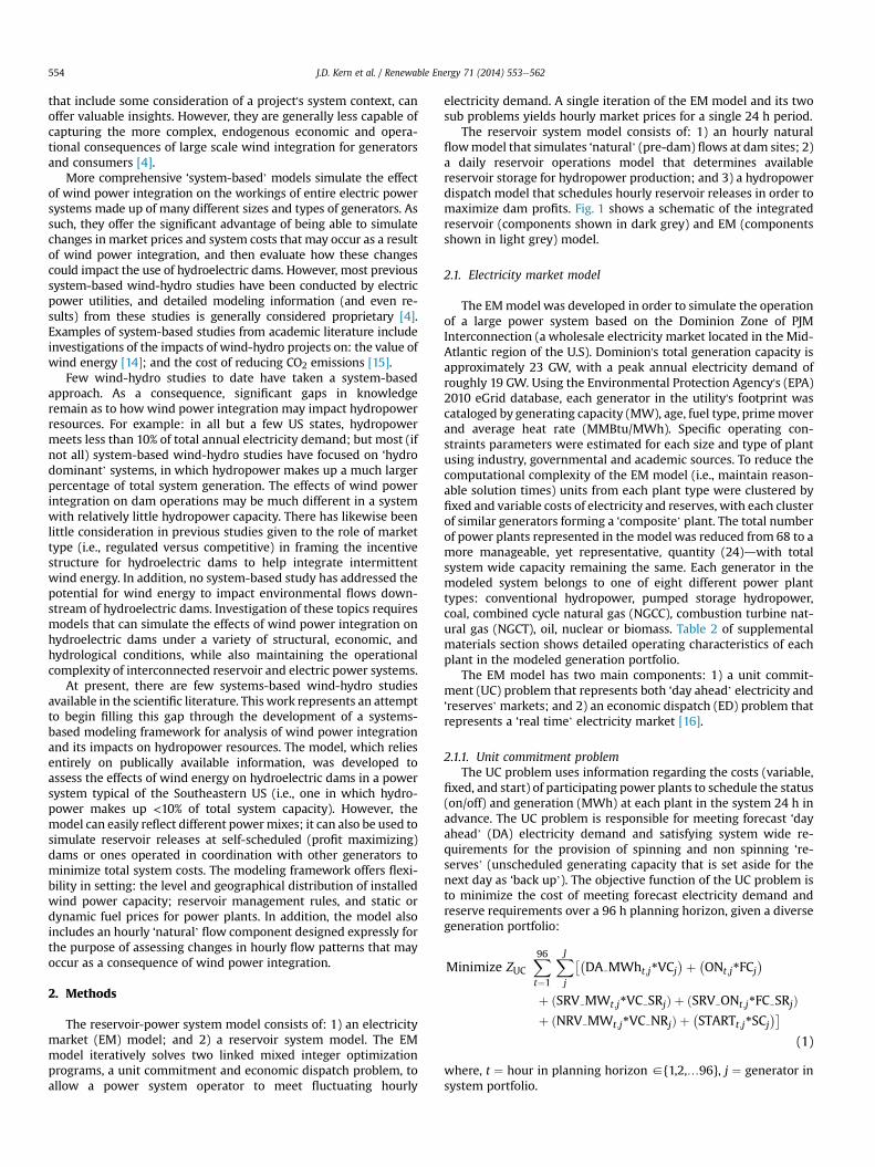
Fig. 6 shows CDFs of mean daily prices for DA (panel A) and RTelectricity (panel B), estimated from the results of a yearlongsimulation that assumed average 2010 fuel prices for coal andnatural gas power plants (of about $1.62/MMBtu, and $4.86/MMBturespectively) [24]. Each panel also indicates the plant type that isdominant in setting the hourly market clearing price for eachsection of the CDF. Panel A shows that a modest amount (i.e., 5%market penetration) of low cost wind energy reduces the marketshare of combined cycle natural gas (NGCC) generators in the DAelectricity market, which results in less expensive coal generatorssetting the market clearing price more often. At 25% wind pene-tration, however, the system relies much more on NGCC generatorsin order to accommodate lower, more volatile net electricity de-mand patterns and increased demand for spinning reserves; as aresult, NGCC units more frequently set the market clearing price

and the bottom 2/3 of the cumulative probability distribution in-creases in value. At the same time, 25% wind market penetrationreduces the frequency of DA price spikes (e.g., especially thosecaused by periods of peak summer demand) associated with theuse of more expensive oil and combustion turbine natural gasgenerators. Thus, panel A shows that the upper quartile of the DAprice distribution is reduced at 25% wind penetration.

In the RTelectricity market (Fig. 6, panel B) wind energy has twomain effects on prices: 1) positive wind forecast errors offset othersources of RT electricity demand and result in more frequent hourswith an RT price of $0/MWh; and 2) negative wind forecast errorsincrease RT electricity demand and cause more frequent occur-rences of high RT prices. Particularly at 25% market penetration,wind energy causes the bottom portion of the cumulative proba-bility distribution function for RT prices to decrease, while the tophalf increases.

In order to illustrate the ability of the integrated model to cap-ture changes in dam operations and revenues as a consequence ofwind power integration, results are also presented from the hy-dropower dispatchmodel under 0%, 5%, and 25% average daily windmarket penetration (i.e., here Roanoke Rapids Dam is assumed tobe a self-scheduled, profit maximizing entity). Fig. 7 shows that at0% wind market penetration, the ratio of total annual DA electricityto reserves sold is roughly 8:5 in favor of the DAmarket. At 5% windmarket penetration, Roanoke Rapids Dam sells slightly more re-serves and RT electricity and less DA electricity. Average prices ineach market decrease due to wind energy's effect on the marketshare of NGCC plants, and annual profits at the dam decrease from$US 8.13 million at baseline to $US 7.81 million at 5% windpenetration.

At 25% wind market penetration, average prices in each marketincrease due to increasedmarket share of NGCC plantsdand profitsat the dam increase to $US 9.44 million. More severe negative windforecast errors entice the dam to significantly increase its sale ofreserves and RT electricity on an annual basis, resulting in a sales

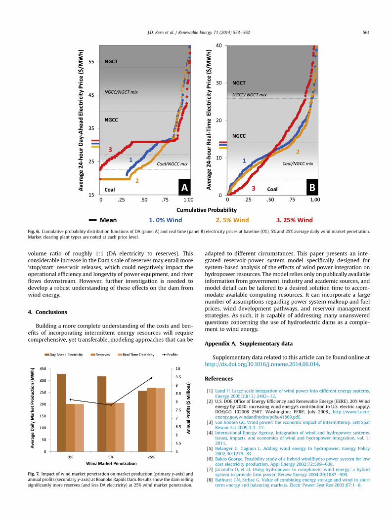
Fig. 6. Cumulative probability distribution functions of DA (panel A) and real time (panel B) electricity prices at baseline (0%), 5% and 25% average daily wind market penetration.Market clearing plant types are noted at each price level.

J.D. Kern et al. / Renewable Energy 71 (2014) 553e562 561

volume ratio of roughly 1:1 (DA electricity to reserves). Thisconsiderable increase in the Dam's sale of reserves may entail more‘stop/start’ reservoir releases, which could negatively impact theoperational efficiency and longevity of power equipment, and riverflows downstream. However, further investigation is needed todevelop a robust understanding of these effects on the dam fromwind energy.

4. Conclusions

Building a more complete understanding of the costs and ben-efits of incorporating intermittent energy resources will requirecomprehensive, yet transferable, modeling approaches that can be

Fig. 7. Impact of wind market penetration on market production (primary y-axis) andannual profits (secondary y-axis) at Roanoke Rapids Dam. Results show the dam sellingsignificantly more reserves (and less DA electricity) at 25% wind market penetration.

adapted to different circumstances. This paper presents an inte-grated reservoir-power system model specifically designed forsystem-based analysis of the effects of wind power integration onhydropower resources. Themodel relies only on publically availableinformation from government, industry and academic sources, andmodel detail can be tailored to a desired solution time to accom-modate available computing resources. It can incorporate a largenumber of assumptions regarding power system makeup and fuelprices, wind development pathways, and reservoir managementstrategies. As such, it is capable of addressing many unansweredquestions concerning the use of hydroelectric dams as a comple-ment to wind energy.

Appendix A. Supplementary data

Supplementary data related to this article can be found online athttp://dx.doi.org/10.1016/j.renene.2014.06.014.

References

[1] Lund H. Large scale integration of wind power into different energy systems.Energy 2005;30(13):2402e12.

[2] U.S. DOE Office of Energy Efficiency and Renewable Energy (EERE). 20% Windenergy by 2030: increasing wind energy's contribution to U.S. electric supply.DOE/GO 102008 2567. Washington: EERE; July 2008., http://www1.eere.energy.gov/windandhydro/pdfs/41869.pdf.

[3] van Kooten GC. Wind power: the economic impact of intermittency. Lett SpatResour Sci 2009;3:1e17.

[4] International Energy Agency. Integration of wind and hydropower systems.Issues, impacts, and economics of wind and hydropower integration, vol. 1;2011.

[5] Belanger C, Gagnon L. Adding wind energy to hydropower. Energy Policy2002;30:1279e84.

[6] Bakos George. Feasibility study of a hybrid wind/hydro power system for lowcost electricity production. Appl Energy 2002;72:599e608.

[7] Jaramillo O, et al. Using hydropower to compliment wind energy: a hybridsystem to provide firm power. Renew Energy 2004;29:1887e909.

[8] Bathurst GN, Strbac G. Value of combining energy storage and wind in shortterm energy and balancing markets. Electr Power Syst Res 2003;67:1e8.

J.D. Kern et al. / Renewable Energy 71 (2014) 553e562562

[9] Angarita JM, Usaola JG. Combining hydro generation and wind energy. Biddingand operation on electricity spot markets. Electr Power Syst Res2007;77(5e6):393e400.

[10] Fernandez Alisha, Blumsack Seth, Reed Patrick. Evaluating wind following andecosystem services for hydroelectric dams. J Regulat Econ 2012;41(1):139e54. http://dx.doi.org/10.1007/s11149-011-9177-9.

[11] Castronuovo E, Lopes JA. On the optimization of the daily operation of a wind-hydro power plant. IEEE Trans Power Syst August 2004;19(3).

[12] Matevosyan J, et al. Hydropower planning coordinated with wind power inareas with congestion problems for trading on the spot and the regulatingmarket. Electr Power Syst Res 2009;79:39e48.

[13] Fernandez Alisha, Blumsack Seth, Reed Patrick. Operating constraints andhydrologic variability limit hydropower in supporting wind integration. En-viron Res Lett 2013;8(2).

[14] Vogstad K. Utilising the complementary characteristics of wind power andhydropower through coordinated hydro production scheduling using theEMPS model. Department of Electrical Eng NTNU; 2003.

[15] Scorah H, et al. The economics of storage, transmission and drought: inte-grating variable wind power into spatially separated electricity grids. EnergyEcon 2012;34(2):536e41.

[16] Kirschen Daniel, Strbac Goran. Fundamentals of power system economics.Wiley Publishing; 2004.

[17] National Renewable Energy Laboratory. Eastern wind integration and trans-mission study; 2011.

[18] Hoppock D, Echeverri D. Cost of wind energy: comparing distant wind re-sources to local resources in the midwestern united states. Environ SciTechnol 2010;44(22):8758e65.

[19] PJM Interconnection. DA energy market. Website: http://www.pjm.com/markets and operations/energy/DA.aspx. [accessed 10.10.12].

[20] EnerNex Corporation. Final report e 2006 Minnesota wind integration study;2006.

[21] Gooi HB, et al. Optimal scheduling of spinning reserve. IEEE Trans Power SystNovember 1999;14(4):1485e92.

[22] Knapp C. The generalized correlation method for estimation of time delay.IEEE Trans Acoust Speech Signal Process 1976;24(4):320e7.

[23] Kern J, Characklis G, Doyle M, Blumsack S, Whisnant R. Influence of deregu-lated electricity markets on hydropower generation and downstream flowregime. J Water Resourc Plan Manage 2012;138(4):342e55.

[24] Energy Information Administration. Website: http://www.eia.gov; September2012.