an interactive simulation environment for...

VOL. 9, NO. 1, JANUARY 2014 ISSN 1990-6145

ARPN Journal of Agricultural and Biological Science ©2006-2014 Asian Research Publishing Network (ARPN). All rights reserved.

www.arpnjournals.com

24

AN INTERACTIVE SIMULATION ENVIRONMENT FOR EVALUATING MANAGERIAL DECISIONS IN A

SUGARCANE PLANTATION IN MEXICO

Enrique Arjona,1 Víctor Perez1, Graciela Bueno1 and Luis Salazar2 1Colegio de Postgraduados, Montecillo, Edo. de Mex., Mexico

2Universidad Tecnologica del Valle del Mezquital, Ixmiquilpan, Hgo., Mexico E-Mail: [email protected]

ABSTRACT

We developed a discrete event simulation environment of the harvesting, transportation and cane processing systems of a sugarcane plantation in Mexico. The purpose of the environment is to help managers to plan and evaluate immediate and mediate actions with a tool that incorporates powerful technological and methodological advances. Simulations are highly interactive and the supporting model can be easily modified at runtime to adjust and test temporary policies. Simulated time can be adjusted to mimic real time allowing the environment to behave as a high-fidelity simulator. Data initialization and runtime user interactions are done through the use of visual components and formal sums of objects. The environment is particularly valuable for the analysis of transient and stationary states, identifying bottlenecks, and obtaining optimum numbers of personnel and machinery. The supporting model includes all the activities that occur from the burning of the cane to its processing in the mill. In a typical day simulation, more than one thousand workers and about two hundred machines are involved. With the environment, several new possible ferry policies in the plantation were statistically evaluated finding one that decreases the daily total processing time in about 7% using the existing machinery. Keywords: sugarcane, managerial decisions, discrete simulation, computer-aided analysis. 1. INTRODUCTION

Planning managerial decisions in a sugarcane plantation during the sugar-making season is very complex. The combinatory of personnel and machinery is very large. Managerial decisions include daily planning of areas to harvest, and allocating labor and machinery for burning, trimming, heaping, loading, and delivering the cane from the plantation to the mill yard. Harvesting occurs simultaneously in separate, often distant sections of the plantation, making it hard to share machinery among sections. Machinery and cane are transported over local roads in riparian areas where few bridges exist; it must often be ferried across rivers. Finally, sugarcane must be harvested within certain periods of plant maturity and, once trimmed; the cane should be milled within 24 hours to preserve weight, saccharose content and juice quality.

Simulation modeling of the sugar cane logistic supply chain has been done using diverse approaches. Hansen et al. (2002) developed a model to study methods of reducing harvest to mill delays. Higgins and Davies (2005) developed a capacity planning model to estimate transport, shifts and delays in harvesting operation. Ianoni and Morabito (2006) studied the reception area processes of a sugar cane plant, analyzing the performance of the system and investigating alternative configurations and policies for its operations. Guan et al. (2008) developed a hybrid continuous-discrete model based on Petri nets where the continuous part models the work in the farm land and the discrete part represents the status changes in resources. Lejars et al. (2008) developed the simulation tool MAGI to help sugarcane growers and millers in designing and assessing new ways of organizing cane supply management within a mill area. Le Gal et al.

(2009) coupled the MAGI model with a daily logistic model to explore the relationship between the two models. Assis et al. (2010) developed a model to analyze the variation of the profit of the sugarcane load transported to the mill, considering the variation of freight and discount applied in relation to the lead time.

On the other hand, object-oriented and real-time simulation modeling technologies have been applied to specific processes of agricultural systems. Villani et al. (2004) developed an object-oriented hybrid model of cane processing using Petri nets and differential equations. Piewthongngam et al. (2009) integrated a simulation model with a mathematical one to optimize sugar production taking in consideration cane supply and mill capacity in a plantation. Parthanadee and Buddhakulsomsiri (2010) used a simulation model to derive real-time dispatching rules in agricultural industries which perform their production schedule in advance in a weekly basis and that have a high interdependence of shared resources. Hameed et al. (2012) developed an object-oriented model of agricultural in-field machinery activities that allows very detailed representation of complex operations.

The simulation environment presented in this paper comprises the harvesting, transportation and cane processing systems of a sugarcane plantation in Mexico and is very different from the tools and models above cited. It is object-oriented but was entirely developed with a RAD tool (see section 2.5 below). It is highly interactive and of a very high level of abstraction. Its supporting model includes all the activities that occur from the burning of the cane to its processing in the mill and the user has total control of the model components at runtime.




25

The model has a one to one correspondence with the discrete components of the plantation so the evolution of the supply logistics in the plantation can be observed in detail by means of dynamic plots and very easy to follow reports. Simulated time can be adjusted to mimic real time allowing the environment to behave as a high-fidelity simulator. In a typical day simulation more than one thousand workers and about two hundred machines are involved. 2. MATERIALS AND METHODS 2.1. The sugarcane plantation

The simulation environment was developed for a sugar plantation in the state of Veracruz, on the Gulf Coast of Mexico where the climate is warm and humid. Annual average temperature is 30ºC. Annual precipitation is 900-1200 mm. Rain season is from May to October, with July being the rainiest month. On average some 3,200 t/d of cane are harvested and milled on the plantation. The sugar-making season begins in middle November or early December and ends in early May lasting about 171 days. The plantation is divided into seven sections; each section integrates several small, rural communities. Three of the roads that connect the sections and the mill yard merge at a river crossing served by a ferry. Most of the cane is trimmed manually; heaping and loading are wholly mechanized. The plantation has an average labor force of about 1, 200, 2 mechanical harvesters, 19 loaders, 113 trucks and 48 tractors and wagons. Each section of the plantation is assigned a weekly amount of cane to harvest, based on estimated saccharose content. Weekly plans for allocating labor and machinery are made accordingly. 2.2. Activity models

As the core of the simulation environment is an activity dynamic model (Poole and Szymankiewicz, 1977; Kreutzer, 1986, Banks et al., 2001), following, we briefly describe the generalities of activity models. These generalities comprise several improvements to the original activity simulation modeling paradigm.

Components of an activity model are entities, waiting lines, activities, and entity flows. Entities represent the physical or logical components of the system and may have attributes. When an activity model is

executed, entities move from waiting lines to activities and vice-versa. Entities in waiting lines are inactive. At the beginning of an activity, the entities required for the activity are taken from the waiting lines. When an activity is in progress, some taken entities may be modified, others may be consumed, and new entities may be generated. At the ending of an activity those entities that were not consumed become inactive and are stored in the waiting lines. Activities may start any time (whenever the entities required by them are available in the appropriate waiting lines).

The number of entities required to start an activity may be constant or variable. There may be several choices of entities required in an activity and of waiting lines from which the entities are taken. Entities required for an activity may be constrained to specific positions in the waiting lines or to meet attribute conditions. Attribute conditions may be absolute or relative to attribute values of others entities required by the activity. The duration of an activity may be constant or variable. Activity durations may depend on attribute values of the entities that participate in the activity and on theoretical or empirical distributions. At the end of an activity, entities may be stored in any of several waiting lines and at specific positions in those lines.

Finally, activities can have access to global variables as the current simulation time and the duration of an activity. 2.3. The support model

The support model is an object-oriented totally interactive activity simulation model, roughly based in a batch model of the harvesting and transportation systems of the plantation developed several years ago and that proved to be very useful for analyzing amortization problems (Arjona et al., 2001).

As mentioned in the introduction, the model covers the harvesting, transportation and cane processing systems of the plantation. The model has a one to one correspondence with the discrete components of the plantation and includes all the activities that occur from the burning of the cane to its processing in the mill. Figure-1 depicts harvesting, and Figure-2 transportation and processing (a system that sometimes causes bottlenecks in transportation).




26

Figure-1. Activity model of the plantation harvesting system.

Figure-2. Activity model of the plantation transportation and processing systems.

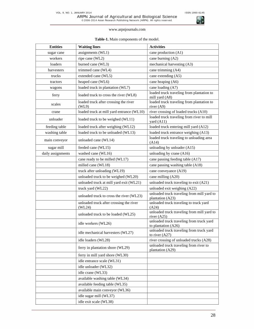
Rectangles represent activities, circles represent waiting lines, and directed arcs represent flows of entities. Each entity represents a physical or logical component of the system (raw materials, machinery, workers, orders, products, etc.). The main entities, waiting lines, and activities of the model are given in Table-1. (For clarity, components used for scheduling, blocking, alternative

operation policies, handling of failures and information flows were not listed. Some of those components appear in Figure-1 as empty boxes and circles).

Each activity has specific flow conditions, attribute modifications and duration. For example, the activity "river crossing of loaded trucks" (A10) requires the following entities:




27

An inactive ferry in the plantation shore (WL29). Three to five loaded trucks waiting to cross the river

(WL8). These entities do not have to meet any condition on their attributes. At the beginning of the activity they are taken from the first positions of the waiting lines. The number of trucks taken will depend only on the availability of trucks in WL8. The activity lasts 22 minutes. No attribute modifications occur at the beginning of this activity. Attribute modifications that occur at the end of the activity are the following: The ferry attribute "number of trips completed," is

increased by 1. The ferry attribute "number of loaded trucks ferried,"

is increased by 3, 4, or 5, depending on the number of trucks that participated in the activity.

For each participating truck, the truck attribute "lost time awaiting the ferry," is increased by the difference of the starting time of the activity and the value of its attribute "arriving time to the shore".

Finally, at the end of the activity the following occur: The ferry becomes available and momentarily

inactive. This is indicated by storing the ferry at the end of the waiting line "ferry in mill yard shore" (WL30).

The trucks that participated in the activity are momentarily inactive in the mill yard shore, this is indicated by storing the trucks, one by one, at the end of the waiting line "loaded truck after crossing the river" (WL9).

The main outputs of the model are, (1) a point estimate of the total processing time of a given amount of

cane; and (2) dynamic data for charts, plots and reports. These data includes lost time in machinery use and the values of several other variables.

Lost times arise when loaders or trucks are inactive. Loaders become inactive when there is no cane to load or no trucks to be loaded. Trucks become inactive when they are waiting for a loader, a harvester, a ferry, a scale, a crane, or an unloader.

The other values computed by the model are statistics about breakdowns in the cane processing system and statistics about the use of each harvester, loader, truck, and ferry.

The operation of the model is as follows: at the beginning of each simulated day, cane and workers are generated, the trucks are in the truck yard and the other machinery is waiting in the plantation. After generation, the cane is burned, and trimmed manually or mechanically harvested and loaded into trucks (while operating in the plantation, the mechanical harvesters have always a truck at their side). If the cane was trimmed manually, it is also extended manually and after extension, heaped and loaded into trucks by loaders. Once loaded, the cane is transported to the mill yard using direct paths or paths interrupted by the river where loaded trucks have to wait for the ferry, cross the river and continue their travel to the mill yard. In the mill yard, loaded trucks have to wait for availability of the entrance scale and afterwards, for availability of the unloader or the crane. At this point, if some component of the cane processing system breaks down, the unloading process is stopped temporarily and trucks have to wait until the component is fixed. Once unloaded, the trucks go to the exit scale and then; to the plantation or to the truck yard. When returning to the plantation, the trucks that use the paths interrupted by the river have to wait again for the ferry, cross the river, and continue their travel to the plantation. The simulated day ends when all the generated cane is transported and processed in the mill.




28

Table-1. Main components of the model.

Entities Waiting lines Activities sugar cane assignments (WL1) cane production (A1)

workers ripe cane (WL2) cane burning (A2) loaders burned cane (WL3) mechanical harvesting (A3)

harvesters trimmed cane (WL4) cane trimming (A4) trucks extended cane (WL5) cane extending (A5)

tractors heaped cane (WL6) cane heaping (A6) wagons loaded truck in plantation (WL7) cane loading (A7)

ferry loaded truck to cross the river (WL8) loaded truck traveling from plantation to mill yard (A8)

scales loaded truck after crossing the river (WL9)

loaded truck traveling from plantation to river (A9)

crane loaded truck at mill yard entrance (WL10) river crossing of loaded trucks (A10)

unloader loaded truck to be weighed (WL11) loaded truck traveling from river to mill yard (A11)

feeding table loaded truck after weighing (WL12) loaded truck entering mill yard (A12) washing table loaded truck to be unloaded (WL13) loaded truck entrance weighing (A13)

main conveyor unloaded cane (WL14) loaded truck traveling to unloading area (A14)

sugar mill feeded cane (WL15) unloading by unloader (A15) daily assignments washed cane (WL16) unloading by crane (A16)

cane ready to be milled (WL17) cane passing feeding table (A17) milled cane (WL18) cane passing washing table (A18) truck after unloading (WL19) cane conveyance (A19) unloaded truck to be weighed (WL20) cane milling (A20) unloaded truck at mill yard exit (WL21) unloaded truck traveling to exit (A21) truck yard (WL22) unloaded exit weighing (A22)

unloaded truck to cross the river (WL23) unloaded truck traveling from mill yard to plantation (A23)

unloaded truck after crossing the river (WL24)

unloaded truck traveling to truck yard (A24)

unloaded truck to be loaded (WL25) unloaded truck traveling from mill yard to river (A25)

idle workers (WL26) unloaded truck traveling from truck yard to plantation (A26)

idle mechanical harvesters (WL27) unloaded truck traveling from truck yard to river (A27)

idle loaders (WL28) river crossing of unloaded trucks (A28)

ferry in plantation shore (WL29) unloaded truck traveling from river to plantation (A29)

ferry in mill yard shore (WL30) idle entrance scale (WL31) idle unloader (WL32) idle crane (WL33) available washing table (WL34) available feeding table (WL35) available main conveyor (WL36) idle sugar mill (WL37) idle exit scale (WL38)




29

2.4. Visual components and formal sums The simulation environment combines visual

components with formal sums. Visual components are used to denote user actions. Formal sums are used for the model description, model initialization, and simulation monitoring.

Visual components are programmed objects that are used in many Windows applications. Many of them as buttons, scrollbars, etc. are familiar to most users. Visual components have a common characteristic: they are very easy to master.

Formal sums are textual components similar to algebraic sums. They provide an explicit compact way to reference entities. In formal sums, operands are entities, and parentheses, triangular brackets, square brackets and braces have a dual function: to delimit an entity with their attributes, and to indicate the way in which an entity is retrieved from or stored in a waiting line or to indicate if the retrieving of the entity is optional. Only attributes of interest are specified in a formal sum, all the others are implicitly given. Use of capital letters is optional and makes no difference in entity or attribute names.

In their simpler form, formal sums represent a union of entities without specific characteristics. For example: 2<Truck> + 1<Ferry>

Entities in formal sums can have specific characteristics that are indicated by means of explicit attribute values. These values can be unique or can belong to a range. One or more explicit attribute values may be specified in an entity. Each attribute value is represented by the attribute name, a relational symbol, and a value. Attribute values are separated by commas and written at the right of the entity name inside the entity delimiters. For example: 2<Truck, Cargo=Cane, Load<=7> + 1<Ferry>

Triangular brackets, square brackets and parenthesis are used to represent the way in which an entity is retrieved from or stored in a waiting line. When retrieving entities from a waiting line, triangular brackets are used to retrieve entities from any position, parentheses to retrieve the entities from the head, and square brackets to retrieve entities from the tail. When storing entities in a waiting line, triangular brackets or parentheses are used to store entities in the head and square brackets to store entities in the tail. For example, in the formal sum: 1[Truck]

The square brackets indicate that the truck should be retrieved (stored) from (in) the tail of a waiting line.

Finally, braces are used to represent optional entities. For example, in the formal sum: 3<Truck> + 2{Truck} + 1<Ferry>

The braces indicate that two of the trucks are not mandatory, so the number of required trucks is from 3 to 5. 2.5. Programming tools

The environment was implemented in Delphi that is an object-oriented RAD (Rapid Application Development) tool for Windows. Last version is XE2

released in September 2011. The native code generated by Delphi does not need any software support, with the exception of a 32-or 64-bit Windows operating system. 3. RESULTS 3.1. The simulation environment

The simulation environment is highly interactive and of a very high level of abstraction. It comprises an ample set of forms (Windows screens) for input and output. All the forms are interactive and parameters and data of interest can be changed in real or simulated time to analyze the effect of changes. Resources or entities are given as formal sums. Dynamic graphs on performance of activities and on behavior of waiting lines can be obtained as well as detailed reports on segments of the simulation. Random variate generators and automatic statistics collection routines are provided for activities. Replication of activities is implicitly driven by the availability of resources and running data is automatically collected. All results can be stored in files for comparison and later usage.

Following we describe features of some of the forms and how they are used to perform a simulation run and to interact with the support model. Later on, in section 3.3, we will describe two more forms (a chart and a plot forms). 3.1.1. The main form

The main form (see Figure-3) includes two menu bars, a form with two display windows, and several buttons and input boxes. First menu bar includes access to files and help (all model modifications, reports, chart and plots can be saved for later usage). Second menu bar includes the displaying of statistics and dynamic charts and flows. First window displays names of activities in progress as well as their starting and (future) ending times. Second window displays the dynamic contents of all the waiting lines. The lower input boxes are used to specify the ending time of a simulation and the real time between steps that determines how fast is a simulation run. Time between steps can be adjusted to mimic real time allowing the environment to behave as a high-fidelity simulator. The lower buttons are used to start, and to pause and continue a simulation run. 3.1.2. The input and output matrix forms

In an activity model, it is necessary to specify which entities are required to start each activity and where to store those entities when the activities end. Entities required to start an activity are taken from specific waiting lines in determined positions and entities released at the end of an activity are stored in specific waiting lines in determined positions.

In the environment, input and output requirements of all the activities of the support model are given as sparse matrices whose non-null elements are formal sums of entities. Matrix rows correspond to activities and columns to waiting lines. In the input matrix, the row of a non-null element indicates which activity




30

requires the formal sum, and the column the waiting line from where the formal sum must be taken. In the output matrix, the row of a non-null element indicates which activity will release the formal sum and the column the waiting line where the formal sum must be stored. As was mentioned in section 2.4, entity delimiters indicate the position where the entity will be taken or stored and if the entity is optional. For example, if the formal sum:

(Scale) + (Truck)

is the element stored internally in the position (2, 3) of an input matrix, then the formal sum (one scale and one truck) should be taken from the head of the waiting line number 3 to start activity 2. Activity and waiting line numbering are done automatically by the environment (when they are defined using the first and second buttons of the main form) and the users do not need to remember their numbers because access to activities and waiting lines is by name.

Figure-3. Main form.

Input and output matrices can be accessed with the third and fourth buttons of the main form. Once a matrix form is accessed, their elements can be easily accessed by selecting the names of an activity (row) and of a waiting line (column) from scroll-down lists, and

modified to test new alternatives for the input/output of activities. This can be done before or during a pause of the simulation. In this later case, modifications will take effect immediately from the time point where the simulation was paused (see Figure-4).

Figure-4. Input matrix form.




31

3.1.3. Attribute modifications form With respect to entity attribute modifications that

happen in activities, the environment provides a form see

Figure-5 supported by an internal interpreter. The form is accessed with the sixth button of the main form.

Figure-5. Attribute modifications form.

Activities are selected with an IF-ENDIF sentence and attribute modifications are specified using functional expressions. Functional expression combine provided functions and global variables. Specification of an attribute modification includes the entity name, the attribute name and the new value of the attribute. For example, the function call: ASSIGN_STRING_VALUE (‘Truck’, ‘Direction’, ‘Mill yard’); makes the assignment: Direction of truck = Mill yard.

Provided functions can be nested to access attribute values of the entities that participate in the activity. For example the function call: ASSIGN_VALUE (‘Truck’, ‘Hours accumulated’, GET_VALUE (‘Truck’, ‘Hours accumulated’) + Activity Duration); increases the hours accumulated of the truck by the activity duration. In this case Activity Duration is a global variable that depends of the activity accessed and that is automatically updated by the internal interpreter.

As in the case of input and output matrices, attribute modifications in activities can be modified before or during a pause of the simulation and modifications will take effect immediately from the time point where the simulation was paused.

The second menu bar of the attribute modifications form allows printing or saving the modifications done in a file for its later use. 3.1.4. Initial waiting lines content form

This form is accessed with the first button of the main form. When the model is been initialized, this form requires the typing of the formal sums that describe the initial contents of the waiting lines (see Figure-6). These entities and their instances will be defined and created dynamically at run-time at the beginning of a simulation run. Entity attributes included in the formal sums are only those that need a specific initialization. Other entity attributes can be defined and initialized dynamically when activities are performed. Entities and their instances can also be defined and created (or consumed) dynamically when an activity ends. 3.1.5. Simulation report form

This form (see Figure-7), which is displayed with the last icon of the second bar menu in the main form, is used for displaying a monitoring report of the simulation runs. The report includes starting and ending times of each activity executed and the movement of entities resulting from each activity execution. Each entity is included with all its attribute values. The report can be complete or




32

partial depending on which of the last two input boxes of the main form is selected. Selection of these boxes can be changed at any time during a simulation run, so the user

interactively decides which time periods of the simulation run must be included in the report.

Figure-6. Initial waiting lines content form.

Figure-7. Simulation report form. 3.2. Data collection, distribution fitting, and validation of the environment

Field data were collected over two years during the sugar-making season. Some data were collected daily, others every other week, and a few in a single day. Data collected daily included: amount of cane to harvest, amount of cane harvested, amount of cane harvested by each harvester, amount of cane loaded by each loader,

amount of cane transported by each truck, time of occurrence and duration of breakdowns in cane processing, and rains. Data collected every other week were: waiting times of trucks in the plantation, loading times of trucks, round trip times of trucks from the plantation to the mill yard, waiting times of trucks in the mill yard, waiting times of trucks at the shore, productivity




33

of workers in harvesting work. Data collected in a single day were data about processing times in the mill.

Activity durations of the supporting model were determined analyzing most of the field collected data. The remaining data was reserved for validation. Some activity durations were considered as constants. Loading times were considered to be gamma random variables and the amount of loaded cane was considered proportional to the loading time. Mechanical harvesting times were also considered to be gamma random variables and the amount of cane harvested was considered proportional to the harvesting time. The theoretical distributions were fitted using Chi-square tests at significance levels of 5%. The proportional factors were determined from the data collected using regression analysis. Traveling times were considered to follow empirical distributions obtained directly from the data collected. Processing times were considered constant except for the case of breakdowns, the durations of which were added to the processing times.

The environment was validated using the part of the data collected that was not used for distribution fitting. We performed two sets of 15 replications, each replication corresponding to a working day. The differences between the total processing times of the plantation and the environment were used to compute confidence intervals for the means of those differences at a 95% confidence level. The intervals included zero, so we considered the validation successful. Actually, outputs from the environment were very consistent with real data, perhaps explained largely by the fact that simulated harvesting and transportation were subdivided into many independent activities whose durations had small and very small variances. So, in the environment as in the real world, the variances of the total processing times were mainly due to the time spent in waiting lines, which in turn depended highly on plantation layout, operation policies and the number of components considered.

3.3. Dynamic outputs To show the graphical utility of the environment,

in Figures 8 to 12 are given examples of the operation of the simulation environment. The purpose of the Figures is to show two dynamic display forms of the environment, one for activity charts and the other for waiting line content plots. Units correspond to hours of plantation operation. All the examples correspond to real data. Comments on the plots are heuristic because are based on a single run. In section 3.4 we will show statistical experiments done with the environment replicating stochastic runs and changing the operation policies of the plantation.

Figure-8 shows that with only a few hours of operation, the plantation has performed more than two thousand activities. Many of the activities have been performed more than 130 times. In Figures 9 to 11 the interaction between activities can be appreciated by the presence of stationary processes in several of the waiting lines. Figure-9 shows that idle loaders have a very small transient period of about 20 minutes followed by a weak stationarity pattern. The length of the queue oscillates between 2 and 9 and suggests, considering a slack, that the plantation has at most 1 loader in excess. Figure-10 shows that loaded trucks waiting to be weighed have a regular transient period of about three hours followed by a strong stationary pattern. The length of the queue oscillates from 0 to 1 truck except for a few very short periods, so the queue behavior can be considered very satisfactory. Figure-11 shows that unloaded trucks waiting to be loaded have a long transient period of about three hours followed by a strong stationary pattern. This means a lot of truck and driver time wasted. Moreover, the minimum length of the queue is 7 suggesting that the plantation has about 5 trucks in excess. Finally, in Figure-12, it can be appreciated that loaded trucks waiting to cross the river have a small transient period followed by a weak increasing, and actually undesirable, stationary pattern. This suggests the convenience of testing other crossing policies for the ferry.

Figure-8. Dynamic bar graph of number of executions of each one of the activities at time 5.87.




34

3.4 Simulation experiments In Arjona et al. (2001), using the batch

simulation model already mentioned, were presented several statistical analyses of the daily total processing time in the plantation changing the number of resources. The purpose of those analyses was to determine minimum sets of machinery to solve some amortization problems. Several alternatives were found that were considered very satisfactory. All the experiments performed in 2001 that

included varying the number of workers, the daily cane assignments and the number of trucks and workers were replicated in the environment as a sort of cross validation.

However, as the mill still had free times every day with the proposed configuration of the plantation, using the interactive simulation environment developed we explored some changes in the operation policies of the plantation trying to reduce the daily total processing time.

Figure-9. Dynamic plot of waiting line of idle loaders.

Figure-10. Dynamic plot of waiting line of loaded trucks waiting to be weighed.

With the exception of some proposed ferry policies that improved a little the total processing time, all the other policies tested resulted in daily total processing times greater than or statistically equal to the real mean time, so the actual operation policy seemed to be the best.

However, after analyzing the simulation results of the proposed policies for the ferry operation that gave small reductions in the daily processing time, new ferry

policies were proposed. The best of these new proposed policies resulted in a daily total processing time that is about 7% less than the actual processing time. This policy is very different from the actual one.

The actual crossing policy was to cross the river when there are at least 5 trucks waiting to cross the river in the shore where the ferry is (plantation or mill yard) or at least 5 trucks waiting to cross the river in the opposite




35

shore (the ferry has a load capacity of 5 trucks). In this later case, the ferry crosses the river with any number of trucks (0 to 5) waiting in its side and returns with 5 trucks from the opposite shore.

The best proposed policy is to cross the river from the plantation shore with 3 to 5 trucks waiting in this

shore (without taking into consideration trucks waiting in the opposite shore), and to cross the river from the mill yard shore with 1 to 5 trucks waiting in this shore or when there are at least 5 trucks waiting to cross the river in the opposite shore.

Figure-11. Dynamic plot of waiting line of unloaded trucks waiting to be loaded.

Figure-12. Dynamic plot of waiting line of loaded trucks waiting to cross the river.

All simulations performed were terminating and each corresponded to a working day. Proposed policies were based on preliminary runs, analysis of stationary waiting line behavior and real world experience. Each policy simulated was evaluated in terms of its total processing time. Processing time was computed in hours. To estimate total processing times and evaluate policies, for each proposed policy we made 171 independent replications. The differences between the total processing times of each proposed policy and the actual one were used to compute 95% confidence intervals for the means of those differences to identify the policies with a total processing time statistically different from the actual one.

After this, we performed sensitivity analyses using hypothesis tests to determine the total processing time of each one of these policies. Finally, we determined the processing time of the policies as percentages of the actual processing time.

Table-2 depicts the estimated population mean time required to process 3, 200 t of cane (a typical day’s assignment) with 8 of the ferry policies tested. Policies are ordered from greater to lower total processing times given as percentages of the actual processing time. The actual policy appears as the fourth in the Table, the best as the eighth.




36

Table-2. Estimated total processing times of 8 of the ferry policies tested. Processing times are given

as percentages of the actual processing time.

Ferry policy Processing time

1. To cross the river from the plantation or the mill yard shore when there are at least 5 trucks waiting to cross in the shore where the ferry is. 115%

2. To cross the river from the plantation or the mill yard shore when there are at least 3 trucks waiting to cross in the shore where the ferry is. 103%

3. To cross the river from the plantation shore when there are at least 5 trucks waiting to cross in this shore or in the opposite shore. To cross the river from the mill yard shore when there is at least 1 truck waiting to cross in this shore.

100%

4. To cross the river from the plantation or the mill yard shore when there are at least 5 trucks waiting to cross in the shore where the ferry is or in the opposite shore. 100%*

5. To cross the river from the plantation or the mill yard shore when there are at least 3 trucks waiting to cross in the shore where the ferry is or in the opposite shore. 99%

6. To cross the river from the plantation or the mill yard shore when there are at least 3 trucks waiting to cross in the shore where the ferry is or at least 2 in the opposite shore. 96%

7. To cross the river from the plantation shore when there are at least 3 trucks waiting to cross in this shore. To cross the river from the mill yard shore when there is at least 1 truck waiting to cross in this shore.

95%

8. To cross the river from the plantation shore when there are at least 3 trucks waiting to cross in this shore. To cross the river from the mill yard shore when there is at least 1 truck waiting to cross in this shore or there are at least 5 trucks waiting to cross in the opposite shore.

93%**

* Actual policy ** Best policy

4. CONCLUSIONS A highly interactive simulation environment for evaluating managerial decisions in a sugar plantation was developed. Main uses of the environment include the analysis of utilization of personnel and machinery, the analysis of interrelated activities and policies, and the stationarity analysis of processes in the plantation.

The simulation environment support model includes the harvesting, transportation and cane processing systems and is an object-oriented model roughly based on a batch simulation model of the plantation developed in 2001 that proved to be very useful to analyze machinery amortization problems.

In the environment, anytime at runtime, the support model can be modified so the model is not only dynamic in its variables but also in its design. Also, anytime at runtime, all required dynamic plots of single (or groups of) entities in the waiting lines can be observed, compared or printed. The simulation speed can be controlled by the user making possible to analyze interactively run results and if the simulation speed is adjusted to mimic real-time the environment behaves as a high-fidelity simulator.

As all user interactions are done through the use of visual components and formal sums of objects and the supporting model is an activity model, the environment is very easy to master by non-simulation specialists as usually are high level managers.

With the environment, proposed policies for the plantation were tested. The aim of these policies was to

reduce the daily total processing time. As almost all proposed policies tested with the environment led to a greater daily total processing time than the actual one, their testing in the real system would have been very costly and very inconvenient. Moreover, the best policy found, that is a new policy for the ferry operation, is totally different to the actual operating policy and was suggested after many experiments with other unsuccessful and poorly successful policies. In this case the simulation environment proved to be very valuable.

As the support model of the environment can be (easily) dynamically modified, this type of simulation environment can be very useful to prove possible actions in a plantation when breakdowns, weather inclemencies, greater than usual cane supplies, less than usual number of trucks or workers, or some other contingencies happen. In a plantation, as with any complex system, unforeseen contingencies usually happen and to make wrong decisions about which actions to take can be very costly. REFERENCES Arjona E., Bueno G. and Salazar L. 2001. An activity simulation model for the analysis of the harvesting and transportation systems of a sugarcane plantation. Computers and Electronics in Agriculture. 32: 247-264. Assis J.J., Prado A., Rangel L. and Soares D. 2010. A simulation model to evaluate sugarcane supply systems. In: Johansson, B., Jain, S., Montoya-Torres, J. and Hugan, J., Yücesan, (Eds.). Proceedings of the 2010 Winter




37

Simulation Conference. SCS Publishing Co., San Diego. pp. 2114-2125. Banks J., Carson J.S., Nelson B.L. and Nicol D.M. 2001. Discrete-Event System Simulation, 3rd Ed. Prentice Hall Int., N.J. Guan S., Nakamura M., Shikanai T. and Okazaki T. 2008. Hybrid Petri nets modeling for farm work flow. Computers and Electronics in Agriculture. 62: 149-158. Hameed I.A., Bochtis D.D., Sorensen C.G. and Vougioukas S. 2012. An object-oriented model for simulating agricultural in-field machinery activities. Computers and Electronics in Agriculture. 81: 24-32. Hansen A.C., Barnes A.J. and Lyne P.W. 2002. Simulation modeling of sugarcane harvest-to-mill delivery systems. Transactions of the ASABE. 45(3): 531-538. Higgins A. and Davies I. 2005. A simulation model for the capacity planning in sugarcane transport. Computers and Electronics in Agriculture. 47: 85-102. Iannoni A.P. and Morabito R. 2006. A discrete simulation analysis of a logistics supply system. Transportation Research. 42: 191-200. Kreutzer W. 1986. System Simulation Programming Styles and Languages. Addison-Wesley, Great Britain. Lejars C., Le Gal P. and Auzoux S. 2008. A decision support approach for cane supply management within a sugar mill area. Computers and Electronics in Agriculture. 60: 239-249. Le Gal P., Le Masson J., Bezuidenhout C.N. and Lagrange L.F. 2009. Coupled modelling of sugarcane supply planning and logistics as a management tool. Computers and Electronics in Agriculture. 68: 168-177. Parthanadee P. and Buddhakulsomsiri J. 2010. Simulation modeling and analysis for production scheduling using real-time dispatching rules: A case study in canned fruit industry. Computers and Electronics in Agriculture. 70: 245-255. Piewthongngam K., Pathumnakul S. and Setthanan K. 2009. Application of crop growth simulation and mathematical modeling to supply chain management in the Thai sugar industry. Agricultural Systems. 102: 58-66. Poole T. and Szymankiewicz J. 1977. Using Simulation to Solve Problems. McGraw Hill Co., UK. Villani E., Pascal J.C., Miyagi P.E. and Valette R. 2004. Object oriented approach for cane sugar production: modelling and analysis. Control Engineering Practice. 12(10): 1279-1289.

an interactive simulation environment for...

Documents