an introduction to domain decomposition methods
TRANSCRIPT

HAL Id: cel-01100932https://hal.archives-ouvertes.fr/cel-01100932v4
Submitted on 10 Jul 2015 (v4), last revised 17 Mar 2021 (v6)
HAL is a multi-disciplinary open accessarchive for the deposit and dissemination of sci-entific research documents, whether they are pub-lished or not. The documents may come fromteaching and research institutions in France orabroad, or from public or private research centers.
L’archive ouverte pluridisciplinaire HAL, estdestinée au dépôt et à la diffusion de documentsscientifiques de niveau recherche, publiés ou non,émanant des établissements d’enseignement et derecherche français ou étrangers, des laboratoirespublics ou privés.
An Introduction to Domain Decomposition Methods:algorithms, theory and parallel implementation
Victorita Dolean, Pierre Jolivet, Frédéric Nataf
To cite this version:Victorita Dolean, Pierre Jolivet, Frédéric Nataf. An Introduction to Domain Decomposition Methods:algorithms, theory and parallel implementation. Master. France. 2015. cel-01100932v4
An Introduction to Domain Decomposition
Methods: algorithms, theory and parallel
implementation
Victorita Dolean Pierre Jolivet Frederic Nataf
July 10, 2015

2

i
The purpose of this text is to offer an overview of the most popular do-main decomposition methods for partial differential equations (PDE). Thepresentation is kept as much as possible at an elementary level with a spe-cial focus on the definitions of these methods in terms both of PDEs andof the sparse matrices arising from their discretizations. We also provideimplementations written in an open source finite element software. In ad-dition, we consider a number of methods that have not been presented inother books. We think that this book will give a new perspective and thatit will complement those of Smith, Bjørstad and Gropp [175], Quarteroniand Valli [165], Mathew [138] and Toselli and Widlund[184] as well as thereview article [22].
The book is addressed to computational scientists, mathematicians, physi-cists and, in general, to people involved in numerical simulation of par-tial differential equations. It can also be used as textbook for advancedundergraduate/First-Year Graduate students. The mathematical tools neededare basic linear algebra, notions of programming, variational formulation ofPDEs and basic knowledge in finite element discretization.
The value of domain decomposition methods is part of a general needfor parallel algorithms for professional and consumer use. We will focus onscientific computing and more specifically on the solution of the algebraicsystems arising from the approximation of a partial differential equation.
Domain decomposition methods are a family of methods to solve prob-lems of linear algebra on parallel machines in the context of simulation. Inscientific computing, the first step is to model mathematically a physicalphenomenon. This often leads to systems of partial differential equationssuch as the Navier-Stokes equations in fluid mechanics, elasticity systemin solid mechanics, Schrodinger equations in quantum mechanics, Black andScholes equation in finance, Lighthill-Witham equations for traffic, . . . Func-tional analysis is used to study the well-posedness of the PDEs which is anecessary condition for their possible numerical approximation. Numericalanalysis enables to design stable and consistant discretization schemes. Thisleads to discrete equations F (u) = b ∈ Rn where n is the number of degreesof freedom of the discretization. If F is linear, calculate u is a problemof linear algebra. If F is nonlinear, a method for solving is the classicalNewton’s method, which also leads to solving a series of linear systems.
In the past, improving performance of a program, either in speed or inthe amount of data processed, was only a matter of waiting for the nextgeneration processors. Every eighteen months, computer performance dou-bled. As a consequence, linear solver research would take second place to thesearch for new discretization schemes. But since approximately year 2005the clock speed stagnates at 2-3 GHz. The increase in performance is almostentirely due to the increase in the number of cores per processor. All ma-jor processor vendors are producing multicore chips and now every machine
ii
is a parallel machine. Waiting for the next generation machine does notguarantee anymore a better performance of a software. To keep doublingperformance parallelism must double. It implies a huge effort in algorithmicdevelopment. Scientific computing is only one illustration of this generalneed in computer science. Visualization, data storage, mesh generation,operating systems, . . . must be designed with parallelism in mind.
We focus here on parallel linear iterative solvers. Contrary to directmethods, the appealing feature of domain decomposition methods is thatthey are naturally parallel. We introduce the reader to the main classesof domain decomposition algorithms: Schwarz, Neumann-Neumann/FETIand Optimized Schwarz. For each method we start by the continuous for-mulation in terms of PDEs for two subdomains. We then give the definitionin terms of stiffness matrices and their implementation in a free finite ele-ment package in the many subdomain case. This presentation reflects thedual nature of domain decomposition methods. They are solvers of linearsystems keeping in mind that the matrices arise from the discretization ofpartial differential operators. As for domain decomposition methods thatdirectly address non linearities, we refer the reader to e.g. [16] or [17] andreferences therein.
In Chapter 1 we start by introducing different versions of Schwarz algo-rithms at continuous level, having as a starting point H. Schwarz method(see [174]): Jacobi Schwarz Method (JSM), Additive Schwarz Method (ASM)and Restricted Additive Schwarz (RAS) which the default parallel solver inPETSc. The first natural feature of these algorithms are that they are equiv-alent to a Block-Jacobi method when the overlap is minimal. We move onto the algebraic versions of the Schwarz methods. In order to do this, sev-eral concepts are necessary: restriction and prolongation operators as wellas partitions of unity which make possible the global definition. These con-cepts are explained in detail in the case of different type of discretizations(finite difference or finite element) and spatial dimensions. The conver-gence of the Schwarz method in the two-subdomain case is illustrated forone-dimensional problems and then for two-dimensional problems by usingFourier analysis. A short paragraph introduces P.L. Lions algorithm thatwill be considered into details in Chapter 2. The last part of the chapter isdedicated to the numerical implementation by using FreeFem++ [108] forgeneral decompositions into subdomains.
In Chapter 2 we present Optimized Schwarz methods applied to theHelmholtz equation which models acoustic wave propagation in the fre-quency domain. We begin with the two subdomain case. We show theneed for the use of interface conditions different from Dirichlet or Neumannboundary conditions. The Lions and Despres algorithms which are basedon Robin interface conditions are analyzed together with their implementa-tions. We also show that by taking even more general interface conditions,
iii
much better convergence can be achieved at no extra cost compared to theuse of Robin interface conditions. We consider the many subdomain caseas well. These algorithms are the method of choice for wave propagationphenomena in the frequency regime. Such situations occur in acoustics,electromagnetics and elastodynamics.
In Chapter 3 we present the main ideas which justify the use of Krylovmethods instead of stationary iterations. Since Schwarz methods introducedin Chapters 1 and 2 represent fixed point iterations applied to precondi-tioned global problems, and consequently not providing the fastest conver-gence possible, it is natural to apply Krylov methods instead. This providesthe justification of using Schwarz methods as preconditioners rather thansolvers. Numerical implementations and results using FreeFem++ are clos-ing the chapter. Although some part of the presentation of some Krylovmethods is not standard, readers already familiar with Krylov methods mayas well skip it.
Chapter 4 is devoted to the introduction of two-level methods. In thepresence of many subdomains, the performance of Schwarz algorithms, i.e.the iteration number and execution time will grow linearly with the numberof subdomains in one direction. From a parallel computing point of view thistranslates into a lack of scalability. The latter can be achieved by adding asecond level or a coarse space. This is strongly related to multigrid methodsand to deflation methods from numerical linear algebra. The simplest coarsespace which belongs to Nicolaides is introduced and then implemented inFreeFem++.
In Chapter 5, we show that Nicolaides coarse space (see above) is aparticular case of a more general class of spectral coarse spaces which aregenerated by vectors issued from solving some local generalized eigenvalueproblems. Then, a theory of these two-level algorithms is presented. First, ageneral variational setting is introduced as well as elements from the abstracttheory of the two-level additive Schwarz methods (e.g. the concept of stabledecomposition). The analysis of spectral and classical coarse spaces goesthrough some properties and functional analysis results. These results arevalid for scalar elliptic PDEs. This chapter is more technical than the othersand is not necessary to the sequel of the book.
Chapter 6 is devoted to the Neumann-Neumann and FETI algorithms.We start with the two subdomain case for the Poisson problem. Then, weconsider the formulation in terms of stiffness matrices and stress the dualityof these methods. We also establish a connection with block factorizationof the stiffness matrix of the original problem. We then show that in themany subdomains case Neumann-Neumann and FETI are no longer strictlyequivalent. For sake of simplicity, we give a FreeFem++ implementation ofonly the Neumann-Neumann algorithm. The reader is then ready to delveinto the abundant litterature devoted to the use of these methods for solvingcomplex mechanical problems.
iv
In Chapter 7, we return to two level methods. This time, a quite recentadaptive abstract coarse space, as well as most classical two-level methodsare presented in a different light, under a common framework. Moreover,their convergence properties are proven in an abstract setting, providedthat the assumptions of the Fictitious Space Lemma are satisfied. Thenew coarse space construction is based on solving GENeralized Eigenvalueproblems in the Overlap (GenEO). The construction is provable in the sensethat the condition number is given in terms of an explicit formula where theconstants that appear are the maximal number of neighbors of a subdomainand a threshold prescribed by the user. The latter can be applied to abroader class of elliptic equations, which include systems of PDEs such aslinear elasticity even with highly heterogeneous coefficients. From § 7.1 to§ 7.6 , we give all the materials necessary to build and analyze two-levelmethods for Additive Schwarz methods. In section 7.7, we build a coarsespace for one level Optimized Schwarz methods of Chapter 2. It is basedon introducing SORAS algorithm and two related generalized eigenvalueproblems. The resulting algorithm is named SORAS-GenEO-2. Section 7.8is devoted to endow one level Neumann-Neumann algorithm of Chapter 6with a GenEO type coarse space.
In Chapter 8 we introduce the parallel computational framework usedin the parallel version of the free finite element package FreeFem++ whichis currently linked with HPDDM, a C++ framework for high-performancedomain decomposition methods, available at the following URL: https:
//github.com/hpddm/hpddm. For sake of simplicity we restrict ourselves tothe two-level Schwarz methods. Numerical simulations of very large scaleproblems on high performance computers show the weak and strong scala-bilities of the Schwarz methods for 2D and 3D Darcy and elasticity problemswith highly heterogeneous coefficients with billions of degrees of freedom. Aself contained FreeFem++ parallel script is given.
We give in Figure 1, the dependency graph of the various chapters. Forinstance in order to read Chapter 4 it is necessary to be familiar with bothChapters 3 and 1. From this graph, the reader is able to choose his way inreading the book. We suggest some possible partial readings. A reader inter-ested in having a quick and partial view and already familiar with Krylovmethods, may very well read only Chapter 1 followed by Chapter 4. Fornew comers to Krylov methods, reading of Chapter 3 must be intercalatedbetween Chapter 1 and Chapter 4.For a quick view on all Schwarz methods without entering into the technicaldetails of coarse spaces, one could consider beginning by Chapter 1 followedby Chapter 2 and then by Chapter 3 on the use of Schwarz methods aspreconditioners, to finish with Chapter 4 on classical coarse spaces.For the more advanced reader, Chapters 5 and 7 provide the technical frame-work for the analysis and construction of more sophisticated coarse spaces.

v
1 2 3 4 5 6 71−6 77 78 8
Figure 1: Dependency graph of chapters
And last, but not least Chapter 8 gives the keys of parallel implementationand illustrates with large scale numerical results the previously introducedmethods.

vi

Contents
1 Schwarz methods 1
1.1 Three continuous Schwarz Algorithms . . . . . . . . . . . . . . 1
1.2 Connection with the Block Jacobi algorithm . . . . . . . . . . 6
1.3 Discrete partition of unity . . . . . . . . . . . . . . . . . . . . . 9
1.3.1 Two subdomain case in one dimension . . . . . . . . . 10
1d Algebraic setting . . . . . . . . . . . . . . . . . . . . . 10
1d Finite element decomposition . . . . . . . . . . . . . 12
1.3.2 Multi dimensional problems and many subdomains . . 13
Multi-D algebraic setting . . . . . . . . . . . . . . . . . . 13
Multi-D finite element decomposition . . . . . . . . . . 14
1.4 Iterative Schwarz methods: RAS, ASM . . . . . . . . . . . . . 15
1.5 Convergence analysis . . . . . . . . . . . . . . . . . . . . . . . . 16
1.5.1 1d case: a geometrical analysis . . . . . . . . . . . . . . 16
1.5.2 2d case: Fourier analysis for two subdomains . . . . . . 17
1.6 More sophisticated Schwarz methods: P.L. Lions’ Algorithm . 19
1.7 Schwarz methods using FreeFem++ . . . . . . . . . . . . . . . 21
1.7.1 A very short introduction to FreeFem++ . . . . . . . . 21
1.7.2 Setting the domain decomposition problem . . . . . . . 26
1.7.3 Schwarz algorithms as solvers . . . . . . . . . . . . . . . 36
1.7.4 Systems of PDEs: the example of linear elasticity . . . 38
2 Optimized Schwarz methods (OSM) 43
2.1 P.L. Lions’ Algorithm . . . . . . . . . . . . . . . . . . . . . . . . 43
2.1.1 Computation of the convergence factor . . . . . . . . . 45
2.1.2 General convergence proof . . . . . . . . . . . . . . . . . 47
2.2 Helmholtz problems . . . . . . . . . . . . . . . . . . . . . . . . . 50
2.2.1 Convergence issues for Helmholtz . . . . . . . . . . . . . 51
2.2.2 Despres’ Algorithm for the Helmholtz equation . . . . 54
2.3 Implementation issues . . . . . . . . . . . . . . . . . . . . . . . . 57
2.3.1 Two-domain non-overlapping decomposition . . . . . . 58
2.3.2 Overlapping domain decomposition . . . . . . . . . . . 62
2.4 Optimal interface conditions . . . . . . . . . . . . . . . . . . . . 65
2.4.1 Optimal interface conditions and ABC . . . . . . . . . 65
1
2 CONTENTS
2.4.2 Optimal Algebraic Interface Conditions . . . . . . . . . 69
2.5 Optimized interface conditions . . . . . . . . . . . . . . . . . . . 71
2.5.1 Optimized interface conditions for η −∆ . . . . . . . . 71
2.5.2 Optimized IC for Helmholtz . . . . . . . . . . . . . . . . 74
Optimized Robin interface conditions . . . . . . . . . . 77
Optimized Second order interface conditions . . . . . . 79
Numerical results . . . . . . . . . . . . . . . . . . . . . . 81
2.5.3 Optimized IC for other equations . . . . . . . . . . . . . 86
2.6 FreeFem++ implementation of ORAS . . . . . . . . . . . . . . 87
3 Krylov methods 91
3.1 Fixed point iterations . . . . . . . . . . . . . . . . . . . . . . . . 92
3.2 Krylov spaces . . . . . . . . . . . . . . . . . . . . . . . . . . . . . 93
3.2.1 Gradient methods . . . . . . . . . . . . . . . . . . . . . . 96
3.3 The Conjugate Gradient method . . . . . . . . . . . . . . . . . 97
3.3.1 The Preconditioned Conjugate Gradient Method . . . 102
3.4 The GMRES method for non-symmetric problems . . . . . . . 104
3.4.1 The GMRES method . . . . . . . . . . . . . . . . . . . . 106
3.4.2 Convergence of the GMRES algorithm . . . . . . . . . 109
3.5 Krylov methods for ill-posed problems . . . . . . . . . . . . . . 111
3.6 Schwarz preconditioners using FreeFem++ . . . . . . . . . . . 114
4 Coarse Spaces 123
4.1 Need for a two-level method . . . . . . . . . . . . . . . . . . . . 123
4.2 Nicolaides coarse space . . . . . . . . . . . . . . . . . . . . . . . 128
4.2.1 Nicolaides coarse space using FreeFem++ . . . . . . . 129
5 Theory of two-level ASM 135
5.1 Introduction of a spectral coarse space . . . . . . . . . . . . . . 135
5.1.1 Spectral coarse spaces for other problems . . . . . . . . 138
5.2 Variational setting . . . . . . . . . . . . . . . . . . . . . . . . . . 138
5.3 Additive Schwarz setting . . . . . . . . . . . . . . . . . . . . . . 139
5.4 Abstract theory for the two-level ASM . . . . . . . . . . . . . . 143
5.5 Definition and properties of coarse spaces . . . . . . . . . . . . 145
5.5.1 Nicolaides coarse space . . . . . . . . . . . . . . . . . . . 146
5.5.2 Spectral coarse space . . . . . . . . . . . . . . . . . . . . 146
5.6 Convergence theory for ASM with Nicolaides and spectralcoarse spaces . . . . . . . . . . . . . . . . . . . . . . . . . . . . . 149
5.7 Functional analysis results . . . . . . . . . . . . . . . . . . . . . 152
5.8 Theory of spectral coarse spaces for scalar heterogeneous prob-lems . . . . . . . . . . . . . . . . . . . . . . . . . . . . . . . . . . . 153

CONTENTS 3
6 Neumann-Neumann and FETI Algorithms 155
6.1 Direct and Hybrid Substructured solvers . . . . . . . . . . . . . 155
6.2 Two-subdomains at the continuous level . . . . . . . . . . . . . 158
6.2.1 Iterative Neumann-Neumann and FETI algorithms . . 159
6.2.2 Substructured reformulations . . . . . . . . . . . . . . . 161
6.2.3 FETI as an optimization problem . . . . . . . . . . . . 164
6.3 Two subdomains case at the algebraic level . . . . . . . . . . . 165
6.3.1 Link with approximate factorization . . . . . . . . . . . 168
6.4 Many subdomains case . . . . . . . . . . . . . . . . . . . . . . . 169
6.4.1 Remarks on FETI . . . . . . . . . . . . . . . . . . . . . . 172
6.5 Neumann-Neumann in FreeFem++ . . . . . . . . . . . . . . . . 173
6.5.1 FreeFem++ scripts . . . . . . . . . . . . . . . . . . . . . 177
6.6 Non-standard Neumann-Neumann type methods . . . . . . . . 182
6.6.1 Smith normal form of linear systems of PDEs . . . . . 183
6.6.2 An optimal algorithm for the bi-harmonic operator . . 186
6.6.3 Some optimal algorithms . . . . . . . . . . . . . . . . . . 188
7 GenEO Coarse Space 191
7.1 Reformulation of the Additive Schwarz Method . . . . . . . . 192
7.2 Mathematical Foundation . . . . . . . . . . . . . . . . . . . . . . 195
7.2.1 Fictitious Space Lemma . . . . . . . . . . . . . . . . . . 195
7.2.2 Symmetric Generalized Eigenvalue problem . . . . . . 197
7.2.3 Auxiliary lemma . . . . . . . . . . . . . . . . . . . . . . . 202
7.3 Finite element setting . . . . . . . . . . . . . . . . . . . . . . . . 204
7.4 GenEO coarse space for Additive Schwarz . . . . . . . . . . . . 205
7.4.1 Some estimates for a stable decomposition with RASM,2206
7.4.2 Definition of the GenEO coarse space . . . . . . . . . . 208
7.5 Hybrid Schwarz with GenEO . . . . . . . . . . . . . . . . . . . . 211
7.5.1 Efficient implementation . . . . . . . . . . . . . . . . . . 213
7.6 FreeFem++ Implementation . . . . . . . . . . . . . . . . . . . . 215
7.7 SORAS-GenEO-2 . . . . . . . . . . . . . . . . . . . . . . . . . . 220
7.7.1 Symmetrized ORAS method . . . . . . . . . . . . . . . . 220
7.7.2 Two-level SORAS algorithm . . . . . . . . . . . . . . . . 222
7.7.3 Nearly Incompressible elasticity . . . . . . . . . . . . . . 223
7.8 Balancing Neumann-Neumann . . . . . . . . . . . . . . . . . . . 226
7.8.1 Easy Neumann-Neumann . . . . . . . . . . . . . . . . . 227
7.8.2 Neumann-Neumann with ill-posed subproblems . . . . 230
7.8.3 GenEO BNN . . . . . . . . . . . . . . . . . . . . . . . . . 234
7.8.4 Efficient implementation of the BNNG method . . . . 238
8 Implementation of Schwarz methods 239
8.1 A parallel FreeFem++ script . . . . . . . . . . . . . . . . . . . . 239
8.1.1 Three dimensional elasticity problem . . . . . . . . . . 239
8.1.2 Native DDM solvers and PETSc Interface . . . . . . . 243
4 CONTENTS
FreeFem++ interface . . . . . . . . . . . . . . . . 244PETSc interface . . . . . . . . . . . . . . . . . . . 245
8.1.3 Validation of the computation . . . . . . . . . . . . . . . 2468.1.4 Parallel Script . . . . . . . . . . . . . . . . . . . . . . . . 246
8.2 Numerical experiments . . . . . . . . . . . . . . . . . . . . . . . 2528.2.1 Small scale computations . . . . . . . . . . . . . . . . . 2528.2.2 Large Scale Computations . . . . . . . . . . . . . . . . . 253
Strong scaling experiments . . . . . . . . . . . . . . . . . 253Weak scaling experiments . . . . . . . . . . . . . . . . . 257
8.3 FreeFem++ Algebraic Formulation . . . . . . . . . . . . . . . . 259

Chapter 1
Schwarz methods
1.1 Three continuous Schwarz Algorithms
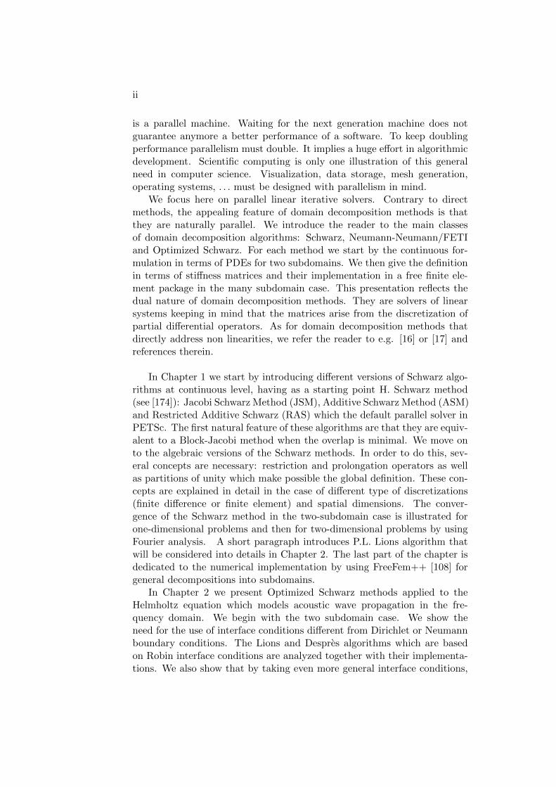
Hermann Schwarz was a German analyst of the 19th century. He was in-terested in proving the existence and uniqueness of the Poisson problem.At his time, there were no Sobolev spaces nor Lax-Milgram theorem. Theonly available tool was the Fourier transform, limited by its very nature tosimple geometries. In order to consider more general situations, H. Schwarzdevised an iterative algorithm for solving Poisson problem set on a union ofsimple geometries, see [174]. For a historical presentation of these kind ofmethods see [88].
Let the domain Ω be the union of a disk and a rectangle, see figure 1.1.Consider the Poisson problem which consists in finding u ∶ Ω→ R such that:
−∆(u) = f in Ωu = 0 on ∂Ω.
(1.1)
Definition 1.1.1 (Original Schwarz algorithm) The Schwarz algorithmis an iterative method based on solving alternatively sub-problems in domains
Ω1 Ω2
Figure 1.1: A complex domain made from the union of two simple geometries
1

2 CHAPTER 1. SCHWARZ METHODS
Ω1 and Ω2. It updates (un1 , un2)→ (un+11 , un+1
2 ) by:
−∆(un+11 ) = f in Ω1
un+11 = 0 on ∂Ω1 ∩ ∂Ω
un+11 = un2 on ∂Ω1 ∩Ω2.
then,
−∆(un+12 ) = f in Ω2
un+12 = 0 on ∂Ω2 ∩ ∂Ω
un+12 = un+1
1 on ∂Ω2 ∩Ω1.(1.2)
H. Schwarz proved the convergence of the algorithm and thus the well-posedness of the Poisson problem in complex geometries.
With the advent of digital computers, this method also acquired a prac-tical interest as an iterative linear solver. Subsequently, parallel computersbecame available and a small modification of the algorithm [128] makes itsuited to these architectures. Its convergence can be proved using the max-imum principle [127].
Definition 1.1.2 (Parallel Schwarz algorithm) Iterative method whichsolves concurrently in all subdomains, i = 1,2:
−∆(un+1i ) = f in Ωi
un+1i = 0 on ∂Ωi ∩ ∂Ω
un+1i = un3−i on ∂Ωi ∩Ω3−i.
(1.3)
It is easy to see that if the algorithm converges, the solutions u∞i , i = 1,2in the intersection of the subdomains take the same values. Indeed, in theoverlap Ω12 ∶= Ω1 ∩Ω2, let e∞ ∶= u∞1 −u∞2 . By the last line of (1.3), we knowthat e∞ = 0 on ∂Ω12. By linearity of the Poisson equation, we also have thate∞ is harmonic. Thus, e∞ solves the homogeneous well-posed boundaryvalue problem (BVP):
−∆(e∞) = 0 in Ω12
e∞ = 0 on ∂Ω12
and thus e∞ = 0 .Algorithms (1.2) and (1.3) act on the local functions (ui)i=1,2. In order
to write algorithms that act on global functions we need extension operatorsand partitions of unity.
Definition 1.1.3 (Extension operators and partition of unity) Let theextension operator Ei such that Ei(wi) ∶ Ω → R is the extension of a func-tion wi ∶ Ωi ↦ R, by zero outside Ωi. We also define the partition of unityfunctions χi ∶ Ωi → R, χi ≥ 0 and χi(x) = 0 for x ∈ ∂Ωi ∖ ∂Ω and such that:
w =2
∑i=1
Ei(χiw∣Ωi) (1.4)
for any function w ∶ Ω↦ R.

1.1. THREE CONTINUOUS SCHWARZ ALGORITHMS 3
There are two ways to write related algorithms that act on global functions.They are given in Definitions 1.1.4 and 1.1.5.
Definition 1.1.4 (First global Schwarz iteration) Let un be an approx-imation to the solution to the Poisson problem (1.1), un+1 is computed bysolving first local sub-problems:
−∆(wn+1i ) = f in Ωi, wn+1
i = un on ∂Ωi ∩Ω3−i
wn+1i = 0 on ∂Ωi ∩ ∂Ω .
(1.5)
and then gluing them together using the partition of unity functions:
un+1 ∶=2
∑i=1
Ei(χiwn+1i ) . (1.6)
We can prove the following property:
Lemma 1.1.1 Algorithm (1.5)-(1.6) which iterates on un and algorithm(1.3) which iterates on (un1 , un2) are equivalent.
Proof Starting from initial guesses which satisfy u0 =2
∑i=1
Ei(χi u0i ), we
prove by induction that
un =2
∑i=1
Ei(χi uni ) . (1.7)
holds for all n ≥ 0. Assume the property holds at step n of the algorithm.Then, using the fact that χ1 = 1 and χ2 = 0 on ∂Ω1∩Ω2 we have by definitionthat wn+1
1 is a solution to BVP (1.3) (with i = 1):
−∆(wn+11 ) = f in Ω1,wn+1
1 = 0 on ∂Ω1 ∩ ∂Ω,
wn+11 = un =
2
∑i=1
Ei(χi uni ) = un2 on ∂Ω1 ∩Ω2.
(1.8)
and thus wn+11 = un+1
1 . The proof is the same for wn+12 = un+1
2 . Finally, wehave using (1.6):
un+1 =2
∑i=1
Ei(χiwni ) =2
∑i=1
Ei(χi uni ) .
This result can be seen as a continuous version of the algebraic formulationestablished in [71].
We introduce in Algorithm 1 another formulation to algorithm (1.5)-(1.6)in terms of the continuous residual rn ∶= f + ∆un. This way, we get closerto the algebraic definition of domain decomposition methods. Algorithm 1is named RAS which stands for Restricted Additive Schwarz.

4 CHAPTER 1. SCHWARZ METHODS
Lemma 1.1.2 (Equivalence between Schwarz’ algorithm and RAS)The algorithm defined by (1.12), (1.13) and (1.14) is called the continuousRAS algorithm. It is equivalent to the Schwarz’ algorithm (1.3).
Proof Here, we have to prove the equality
un = E1(χ1un1) +E2(χ2u
n2) ,
where un1,2 is given by (1.3) and un is given by (1.12)-(1.13)-(1.14). Weassume that the property holds for the initial guesses:
u0 = E1(χ1u01) +E2(χ2u
02)
and proceed by induction assuming the property holds at step n of thealgorithm, i.e. un = E1(χ1u
n1) +E2(χ2u
n2). From (1.14) we have
un+1 = E1(χ1(un + vn1 )) +E2(χ2(un + vn2 )) . (1.9)
We prove now that un∣Ω1
+ vn1 = un+11 by proving that un
∣Ω1+ vn1 satisfies (1.3)
as un+11 does. We first note that, using (1.13)-(1.12) we have:
−∆(un + vn1 ) = −∆(un) + rn = −∆(un) + f +∆(un) = f in Ω1,
un + vn1 = un on ∂Ω1 ∩Ω2,(1.10)
It remains to prove that
un = un2 on ∂Ω1 ∩Ω2 .
By the induction hypothesis we have un = E1(χ1un1) +E2(χ2u
n2). On ∂Ω1 ∩
Ω2, we have χ1 ≡ 0 and thus χ2 ≡ 1. So that on ∂Ω1 ∩Ω2 we have :
un = χ1un1 + χ2u
n2 = un2 . (1.11)
Finally from (1.10) and (1.11) we can conclude that un∣Ω1
+ vn1 satisfies
problem (1.3) and is thus equal to un+11 . The same holds for domain Ω2,
un∣Ω2
+ vn2 = un+12 . Then equation (1.9) reads
un+1 = E1(χ1un+11 ) +E2(χ2u
n+12 )
which ends the proof of the equivalence between Schwarz’ algorithm and thecontinuous RAS algorithm (1.12)-(1.13)- (1.14).
Another global variant of the parallel Schwarz algorithm (1.3) consistsin replacing formula (1.6) by a simpler formula not based on the partitionof unity.
1.1. THREE CONTINUOUS SCHWARZ ALGORITHMS 5
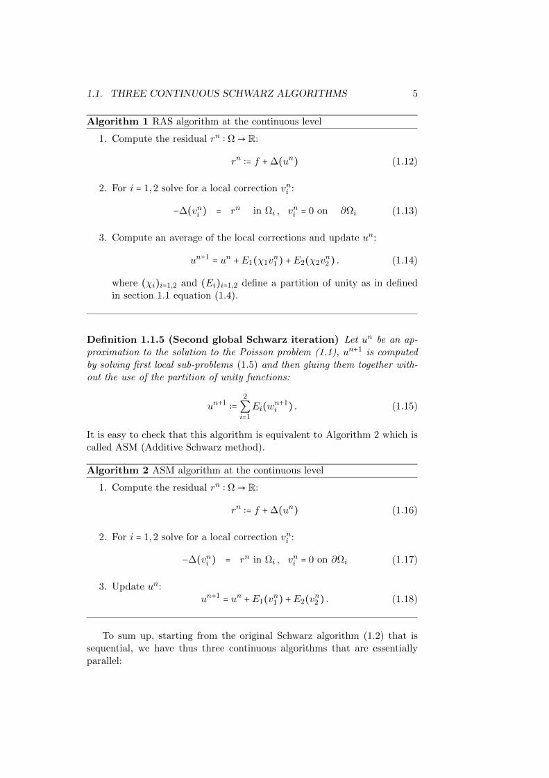
Algorithm 1 RAS algorithm at the continuous level
1. Compute the residual rn ∶ Ω→ R:
rn ∶= f +∆(un) (1.12)
2. For i = 1,2 solve for a local correction vni :
−∆(vni ) = rn in Ωi , vni = 0 on ∂Ωi (1.13)
3. Compute an average of the local corrections and update un:
un+1 = un +E1(χ1vn1 ) +E2(χ2v
n2 ) . (1.14)
where (χi)i=1,2 and (Ei)i=1,2 define a partition of unity as in definedin section 1.1 equation (1.4).
Definition 1.1.5 (Second global Schwarz iteration) Let un be an ap-proximation to the solution to the Poisson problem (1.1), un+1 is computedby solving first local sub-problems (1.5) and then gluing them together with-out the use of the partition of unity functions:
un+1 ∶=2
∑i=1
Ei(wn+1i ) . (1.15)
It is easy to check that this algorithm is equivalent to Algorithm 2 which iscalled ASM (Additive Schwarz method).
Algorithm 2 ASM algorithm at the continuous level
1. Compute the residual rn ∶ Ω→ R:
rn ∶= f +∆(un) (1.16)
2. For i = 1,2 solve for a local correction vni :
−∆(vni ) = rn in Ωi , vni = 0 on ∂Ωi (1.17)
3. Update un:un+1 = un +E1(vn1 ) +E2(vn2 ) . (1.18)
To sum up, starting from the original Schwarz algorithm (1.2) that issequential, we have thus three continuous algorithms that are essentiallyparallel:
6 CHAPTER 1. SCHWARZ METHODS
• Algorithm (1.3) Jacobi Schwarz Method (JSM)
• Algorithm (1.12)-(1.13)-(1.14) Restricted Additive Schwarz (RAS)
• Algorithm (1.16)-(1.17)-(1.18) Additive Schwarz Method (ASM)
The discrete version of the first algorithm is seldom implemented sinceit involves duplication of unknowns. The discrete version of the secondalgorithm is the restricted additive Schwarz method (RAS, see[19, 20]) whichis the default parallel solver in the package PETSC [7]. The discrete versionof the third algorithm is the additive Schwarz method (ASM) for which manytheoretical results have been derived, see [184] and references therein. Thelatter term was introduced first by Dryja and Widlund in [66] for a variantof the algorithm firstly introduced at continuous level in [139].
1.2 Connection with the Block Jacobi algorithm
In the previous section we have noticed that the three methods illustratedifferent points of view of the Schwarz iteration, the continuous aspect em-phasized the interest of the overlap (see § 1.5), which is hidden in the discreteformulation. When going to the discrete level, we will see that Schwarz al-gorithm is, from a linear algebra point of view, a variation of a block-Jacobialgorithm.
We first recall the definition of a block Jacobi algorithm and then es-tablish a connection with the Schwarz algorithms. Let us consider a linearsystem:
AU = F (1.19)
with a matrix A of size m ×m, a right-hand side F ∈ Rm and a solutionU ∈ Rm where m is an integer. The set of indices 1, . . . ,m is partitionedinto two sets
N1 ∶= 1, . . . ,ms and N2 ∶= ms + 1, . . . ,m .
Let U1 ∶= (Uk)k∈N1 ∶= U∣N1, U2 ∶= (Uk)k∈N2 ∶= U∣N2
and similarly F1 ∶= F∣N1,
F2 ∶= F∣N2.
The linear system has the following block form:
( A11 A12
A21 A22)( U1
U2) = ( F1
F2)
where Aij ∶= A∣Ni×Nj, 1 ≤ i, j ≤ 2.
Definition 1.2.1 (Jacobi algorithm) Let D be the diagonal of A, the Ja-cobi algorithm reads:
DUn+1 =DUn + (F −AUn) ,

1.2. CONNECTION WITH THE BLOCK JACOBI ALGORITHM 7
or equivalently,
Un+1 = Un +D−1(F −AUn) = Un +D−1rn ,
where rn = F −AUn is the residual of the equation.
We now define a block Jacobi algorithm.
Definition 1.2.2 (Block-Jacobi algorithm) The block-Jacobi algorithmreads:
( A11 00 A22
)( Un+11
Un+12
) = ( A11 00 A22
)( Un1
Un2
) + ( F1
F2) −A( Un
1
Un2
)
(1.20)or equivalently
⎛⎝A11 0
0 A22
⎞⎠⎛⎝
Un+11
Un+12
⎞⎠=⎛⎝F1 −A12 Un
2
F2 −A21 Un1
⎞⎠. (1.21)
In order to have a more compact form of the previous algorithm, we in-troduce R1 the restriction operator from N into N1 and similarly R2 therestriction operator from N into N2. The transpose operator RTi are exten-sions operators from Ni into N . Note that Aii = RiARTi .
Lemma 1.2.1 (Compact form of a block-Jacobi algorithm) The al-gorithm (1.21) can be re-written as
Un+1 = Un + (RT1 (R1ART1 )−1R1 +RT2 (R2AR
T2 )−1R2) rn . (1.22)
Proof Let Un = (Un1T ,Un
2T )T , algorithm (1.21) becomes
⎛⎝A11 0
0 A22
⎞⎠
Un+1 = F −⎛⎝
0 A12
A21 0
⎞⎠
Un . (1.23)
On the other hand, equation (1.20) can be rewritten equivalently
( Un+11
Un+12
) = ( Un1
Un2
)+( A11 00 A22
)−1
( rn1rn2
)⇔Un+1 = Un+( A−111 00 A−1
22) rn
(1.24)where rni ∶= rn
∣Ni, i = 1,2 . By taking into account that
( A−111 00 0
) = RT1 A−111R1 = RT1 (R1AR
T1 )−1R1
and
( 0 00 A−1
22) = RT2 A−1
22R2 = RT2 (R2ART2 )−1R2 ,
8 CHAPTER 1. SCHWARZ METHODS
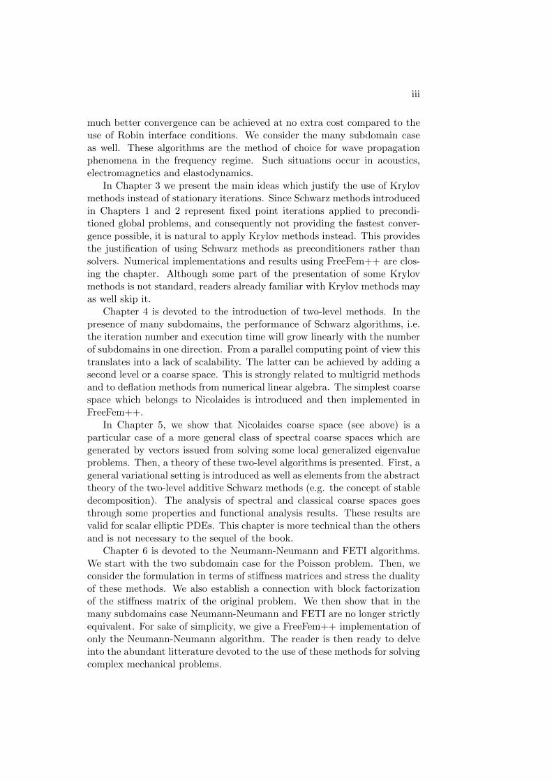
Ω1 Ω2xms xms+1
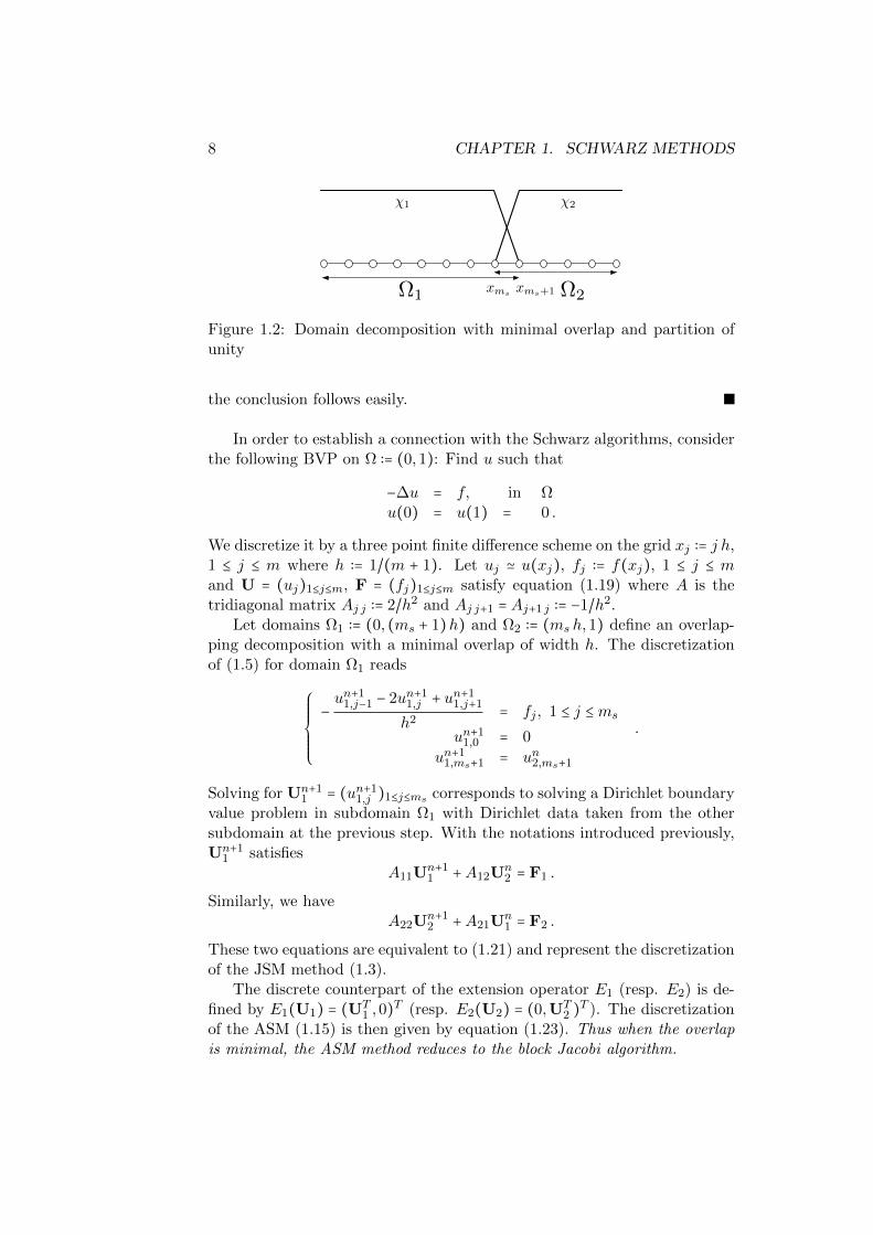
χ1 χ2
Figure 1.2: Domain decomposition with minimal overlap and partition ofunity
the conclusion follows easily.
In order to establish a connection with the Schwarz algorithms, considerthe following BVP on Ω ∶= (0,1): Find u such that
−∆u = f, in Ωu(0) = u(1) = 0 .
We discretize it by a three point finite difference scheme on the grid xj ∶= j h,1 ≤ j ≤ m where h ∶= 1/(m + 1). Let uj ≃ u(xj), fj ∶= f(xj), 1 ≤ j ≤ mand U = (uj)1≤j≤m, F = (fj)1≤j≤m satisfy equation (1.19) where A is thetridiagonal matrix Aj j ∶= 2/h2 and Aj j+1 = Aj+1 j ∶= −1/h2.
Let domains Ω1 ∶= (0, (ms + 1)h) and Ω2 ∶= (ms h,1) define an overlap-ping decomposition with a minimal overlap of width h. The discretizationof (1.5) for domain Ω1 reads
⎧⎪⎪⎪⎪⎪⎨⎪⎪⎪⎪⎪⎩
−un+1
1,j−1 − 2un+11,j + un+1
1,j+1
h2= fj , 1 ≤ j ≤ms
un+11,0 = 0
un+11,ms+1 = un2,ms+1
.
Solving for Un+11 = (un+1
1,j )1≤j≤ms corresponds to solving a Dirichlet boundaryvalue problem in subdomain Ω1 with Dirichlet data taken from the othersubdomain at the previous step. With the notations introduced previously,Un+1
1 satisfiesA11U
n+11 +A12U
n2 = F1 .
Similarly, we haveA22U
n+12 +A21U
n1 = F2 .
These two equations are equivalent to (1.21) and represent the discretizationof the JSM method (1.3).
The discrete counterpart of the extension operator E1 (resp. E2) is de-fined by E1(U1) = (UT
1 ,0)T (resp. E2(U2) = (0,UT2 )T ). The discretization
of the ASM (1.15) is then given by equation (1.23). Thus when the overlapis minimal, the ASM method reduces to the block Jacobi algorithm.
1.3. DISCRETE PARTITION OF UNITY 9
Let χi, i = 1,2 be the piecewise linear functions that define a partitionof unity on the domain decomposition, see Figure 1.2. In this very simpleconfiguration,
χ1(x) =⎧⎪⎪⎨⎪⎪⎩
1 if 0 ≤ x ≤ xmsxms+1 − x
hif xms ≤ x ≤ xms+1
and
χ2(x) =⎧⎪⎪⎨⎪⎪⎩
x − xmsh
if xms ≤ x ≤ xms+1
1 if xms+1 ≤ x ≤ 1.
Functions χi, i = 1,2 define a partition of unity in the sense of (1.4). Sincethe overlap is minimal, the discretization of (1.6) is equivalent to that of(1.15). Thus RAS reduces, in this case, to ASM.
Remark 1.2.1 In conclusion when the overlap is minimal the discrete coun-terparts of the three Schwarz methods of section 1.1 are equivalent to thesame block Jacobi algorithm. Notice here a counter-intuitive feature: a nonoverlapping decomposition of the set of indices N corresponds to a geometricdecomposition of the domain Ω with minimal overlap.
1.3 Algebraic algorithms: discrete partition of unity
Our goal is to introduce in the general case the algebraic counterparts ofalgorithms RAS and ASM defined in § 1.1. The simplest way to do so is towrite the iterative method in terms of residuals as is done in equation (1.22).In order to do this, we need to settle some elements necessary in this writing.One of them is the proper definition of the partition of unity.
At the continuous level (partial differential equations), the main ingre-dients of the partition of unity are
• An open domain Ω and an overlapping decomposition into N opensubsets Ω = ∪Ni=1Ωi.
• A function u ∶ Ω→ R.
• The extension operator Ei of a function Ωi → R to a function Ω → Requals to zero in Ω/Ωi.
• The partition of unity functions χi, 1 ≤ i ≤ N introduced in for-mula (1.4) which verify for all functions u ∶ Ω→ R:
u =2
∑i=1
Ei(χi u∣Ωi).
We can give a similar definition at the discrete level.

10 CHAPTER 1. SCHWARZ METHODS
Definition 1.3.1 (Algebraic partition of unity) At the discrete level,the main ingredients of the partition of unity are
• A set indices of degrees of freedom N and a decomposition into Nsubsets N = ∪Ni=1Ni.
• A vector U ∈ R#N .
• The restriction of a vector U ∈ R#N to a subdomain Ωi, 1 ≤ i ≤ Ncan be expressed as RiU where Ri is a rectangular #Ni×#N Booleanmatrix. The extension operator will be the transpose matrix RTi .
• The partition of unity “functions” at discrete level correspond to diag-onal matrices of size #Ni × #Ni with non negative entries such thatfor all vectors U ∈ R#N
U =N
∑i=1
RTi DiRiU ,
or in other words
Id =N
∑i=1
RTi DiRi (1.25)
where Id ∈ R#N×#N is the identity matrix.
As pointed out in Remark 1.2.1 an overlapping decomposition of a domainΩ might correspond to a partition of the set of indices.
In the following we will give some simple examples where all the ingre-dients of the Definition 1.3.1 are detailed and we will check that (1.25) isverified in those cases.
1.3.1 Two subdomain case in one dimension
1d Algebraic setting
We start from the 1d example of § 1.2 with n = 5, ns = 3 so that the set ofindices N ∶= 1, . . . ,5 is partitioned into two sets, see Figure 1.3
N1 ∶= 1,2,3 and N2 ∶= 4,5 .
Then, matrix R1 is of size 3 × 5 and matrix R2 is of size 2 × 5:
R1 =⎛⎜⎝
1 0 0 0 00 1 0 0 00 0 1 0 0
⎞⎟⎠
and R2 = (0 0 0 1 00 0 0 0 1
) ,

1.3. DISCRETE PARTITION OF UNITY 11
N1 N2
1 2 3 4 5
Figure 1.3: Algebraic partition of the set of indices
and
RT1 =
⎛⎜⎜⎜⎜⎜⎜⎝
1 0 00 1 00 0 10 0 00 0 0
⎞⎟⎟⎟⎟⎟⎟⎠
and RT2 =
⎛⎜⎜⎜⎜⎜⎜⎝
0 00 00 01 00 1
⎞⎟⎟⎟⎟⎟⎟⎠
.
We also have
D1 =⎛⎜⎝
1 0 00 1 00 0 1
⎞⎟⎠
and D2 = (1 00 1
) .
It is clear that relation (1.25) holds.
N δ=11
N δ=12
1 2 3 4 5
Figure 1.4: Algebraic decomposition of the set of indices into overlappingsubsets
Consider now the case where each subset is extended with a neighboringpoint, see Figure 1.4:
N δ=11 ∶= 1,2,3,4 and N δ=1
2 ∶= 3,4,5 .Then, matrices R1 and R2 are:
R1 =⎛⎜⎜⎜⎝
1 0 0 0 00 1 0 0 00 0 1 0 00 0 0 1 0
⎞⎟⎟⎟⎠
and R2 =⎛⎜⎝
0 0 1 0 00 0 0 1 00 0 0 0 1
⎞⎟⎠.
The simplest choices for the partition of unity matrices are
D1 =⎛⎜⎜⎜⎝
1 0 0 00 1 0 00 0 1 00 0 0 0
⎞⎟⎟⎟⎠
and D2 =⎛⎜⎝
0 0 00 1 00 0 1
⎞⎟⎠

12 CHAPTER 1. SCHWARZ METHODS
or
D1 =⎛⎜⎜⎜⎝
1 0 0 00 1 0 00 0 1/2 00 0 0 1/2
⎞⎟⎟⎟⎠
and D2 =⎛⎜⎝
1/2 0 00 1/2 00 0 1
⎞⎟⎠.
Again, it is clear that relation (1.25) holds.
Ω1 Ω2
1 2 3 4 5
Figure 1.5: Finite element partition of the mesh
1d Finite element decomposition
We still consider the 1d example with a decomposition into two subdomainsbut now in a finite element spirit. A partition of the 1D mesh of Figure 1.5corresponds to an overlapping decomposition of the set of indices:
N1 ∶= 1,2,3 and N2 ∶= 3,4,5 .
Then, matrices R1 and R2 are:
R1 =⎛⎜⎝
1 0 0 0 00 1 0 0 00 0 1 0 0
⎞⎟⎠
and R2 =⎛⎜⎝
0 0 1 0 00 0 0 1 00 0 0 0 1
⎞⎟⎠.
In order to satisfy relation (1.25), the simplest choice for the partition ofunity matrices is
D1 =⎛⎜⎝
1 0 00 1 00 0 1/2
⎞⎟⎠
and D2 =⎛⎜⎝
1/2 0 00 1 00 0 1
⎞⎟⎠
Consider now the situation where we add a mesh to each subdomain, seeFigure 1.6. Accordingly, the set of indices is decomposed as:
N δ=11 ∶= 1,2,3,4 and N δ=1
2 ∶= 2,3,4,5 .
Then, matrices R1 and R2 are:
R1 =⎛⎜⎜⎜⎝
1 0 0 0 00 1 0 0 00 0 1 0 00 0 0 1 0
⎞⎟⎟⎟⎠
and R2 =⎛⎜⎜⎜⎝
0 1 0 0 00 0 1 0 00 0 0 1 00 0 0 0 1
⎞⎟⎟⎟⎠.
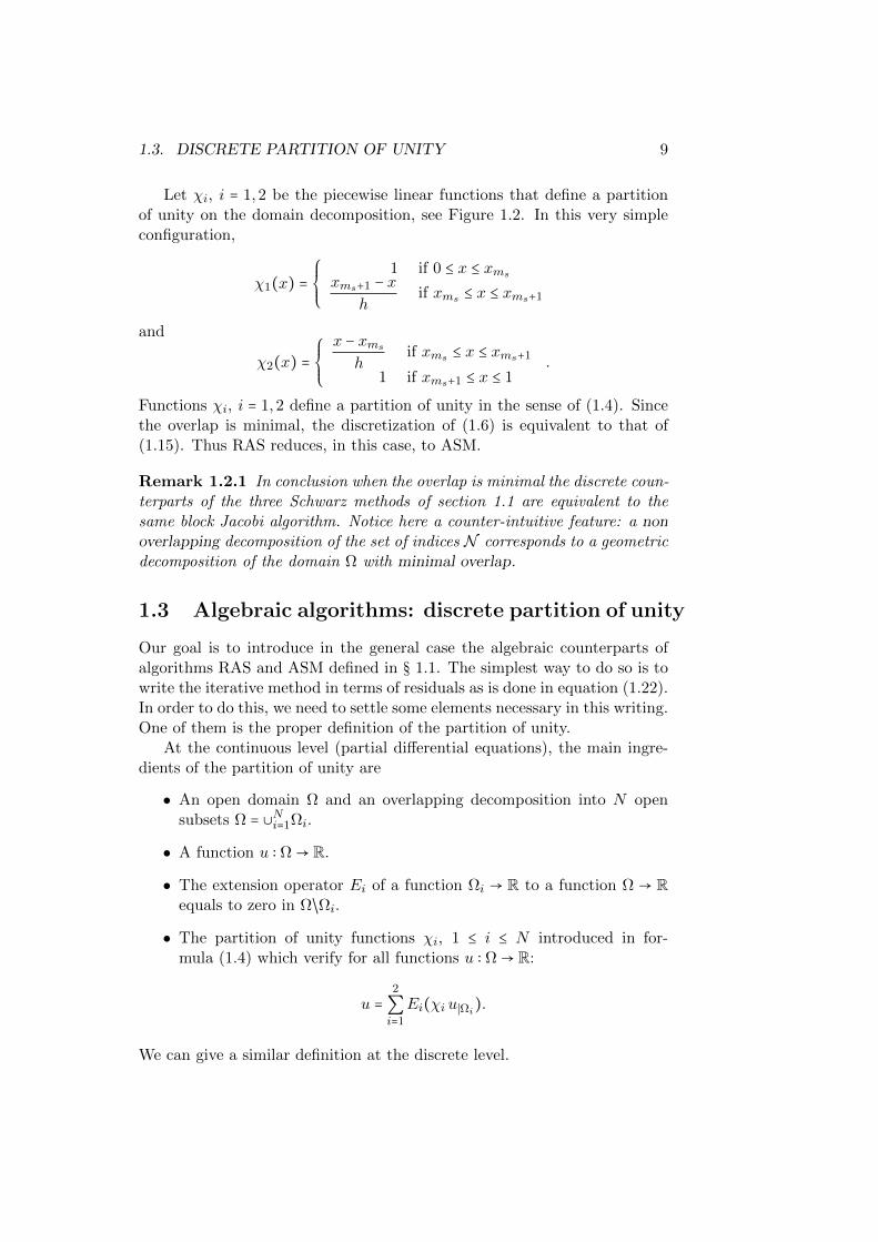
1.3. DISCRETE PARTITION OF UNITY 13
Ωδ=11 Ωδ=1
2
1 2 3 4 5
Figure 1.6: Finite element decomposition of the mesh into overlapping sub-domains
In order to satisfy relation (1.25), the simplest choice for the partition ofunity matrices is
D1 =⎛⎜⎜⎜⎝
1 0 0 00 1 0 00 0 1/2 00 0 0 0
⎞⎟⎟⎟⎠
and D2 =⎛⎜⎜⎜⎝
0 0 0 00 1/2 0 00 0 1 00 0 0 1
⎞⎟⎟⎟⎠.
Another possible choice that will satisfy relation (1.25) as well is
D1 =⎛⎜⎜⎜⎝
1 0 0 00 1/2 0 00 0 1/2 00 0 0 1/2
⎞⎟⎟⎟⎠
and D2 =⎛⎜⎜⎜⎝
1/2 0 0 00 1/2 0 00 0 1/2 00 0 0 1
⎞⎟⎟⎟⎠.
1.3.2 Multi dimensional problems and many subdomains
In the general case, the set of indices N can be partitioned by an automaticgraph partitioner such as METIS[121] or SCOTCH [26]. From the inputmatrix A, a connectivity graph is created. Two indices i, j ∈ N are connectedif the matrix coefficient Aij ≠ 0. Usually, even if matrix A is not symmetric,the connectivity graph is symmetrized. Then algorithms that find a goodpartitioning of the vertices even for highly unstructured graphs are used.This distribution must be done so that the number of elements assigned toeach processor is roughly the same, and the number of adjacent elementsassigned to different processors is minimized (graph cuts). The goal of thefirst condition is to balance the computations among the processors. Thegoal of the second condition is to minimize the communication resultingfrom the placement of adjacent elements to different processors.
Multi-D algebraic setting
Let us consider a partition into N subsets (see Figure 1.7):
N ∶=N
⋃i=1
Ni, Ni ∩Nj = ∅ for i ≠ j . (1.26)

14 CHAPTER 1. SCHWARZ METHODS
Let Ri be the restriction matrix from set N to the subset Ni and Di theidentity matrix of size #Ni × #Ni, 1 ≤ i ≤ N . Then, relation (1.25) issatisfied.
N δ=12
N δ=11
N δ=13N2
N1
N3
Figure 1.7: Partition and overlapping decomposition of the set of indices
Consider now the case where each subset Ni is extended with its directneighbors to formN δ=1
i , see Figure 1.7. Let Ri be the restriction matrix fromsetN to the subsetN δ=1
i and Di be a diagonal matrix of size #N δ=1i ×#N δ=1
i ,1 ≤ i ≤ N . For the choice of the coefficients of Di there are two main options.The simplest one is to define it as a Boolean matrix:
(Di)jj ∶= 1 if j ∈ Ni,0 if j ∈ N δ=1
i /Ni.
Then, relation (1.25) is satisfied. Another option is to introduce for all j ∈ Nthe set of subsets having j as an element:
Mj ∶= 1 ≤ i ≤ N ∣ j ∈ N δ=1i .
Then, define
(Di)jj ∶= 1/#Mj , for j ∈ N δ=1i .
Then, relation (1.25) is satisfied.
Multi-D finite element decomposition
Partitioning a set of indices is well adapted to an algebraic framework. Ina finite element setting, the computational domain is the union of elementsof the finite element mesh Th. A geometric partition of the computationaldomain is natural. Here again, graph partitioning can be used by firstmodeling the finite element mesh by a graph, and then partitioning theelements into N parts (Ti,h)1≤i≤N , see Figure 1.8. By adding to each part

1.4. ITERATIVE SCHWARZ METHODS: RAS, ASM 15
Figure 1.8: Left: Finite element partition; Right: one layer extension of theright subdomain
layers of elements, it is possible to create overlapping subdomains resolvedby the finite element meshes:
Ωi = ⋃τ∈Ti,h
τ for 1 ≤ i ≤ N . (1.27)
Let φkk∈N be a basis of the finite element space. We define
Ni ∶= k ∈ N ∶ supp (φk) ∩Ωi ≠ ∅1 ≤ i ≤ N. (1.28)
For each degree of freedom k ∈ N , let
µk ∶= #j ∶ 1 ≤ j ≤ N and supp (φk) ∩Ωj ≠ ∅ .
Let Ri be the restriction matrix from set N to the subset Ni and Di be adiagonal matrix of size #Ni ×#Ni, 1 ≤ i ≤ N such that
(Di)kk ∶= 1/µk, k ∈ Ni.
Then, relation (1.25) is satisfied.
1.4 Iterative Schwarz methods: RAS, ASM
In a similar way to what was done for the block Jacobi algorithm in equa-tion (1.22), we can define RAS (the counterpart of Algorithm (1.5)-(1.6))and ASM algorithms (the counterpart of Algorithm (1.5)-(1.15)).
Definition 1.4.1 (RAS algorithm) The iterative RAS algorithm is thepreconditioned fixed point iteration defined by
Un+1 = Un +M−1RASrn, rn ∶= F −AUn

16 CHAPTER 1. SCHWARZ METHODS
where the matrix
M−1RAS ∶=
N
∑i=1
RTi Di (RiARTi )−1Ri (1.29)
is called the RAS preconditioner.
Definition 1.4.2 (ASM algorithm) The iterative ASM algorithm is thepreconditioned fixed point iteration defined by
Un+1 = Un +M−1ASMrn, rn ∶= F −AUn
where the matrix
M−1ASM ∶=
N
∑i=1
RTi (RiARTi )−1Ri (1.30)
is called the ASM preconditioner.
1.5 Convergence analysis
In order to have an idea about the convergence of these methods, we performa simple yet revealing analysis. We consider in § 1.5.1. a one dimensionaldomain decomposed into two subdomains. This shows that the size of theoverlap between the subdomains is key to the convergence of the method. In§ 1.5.2 an analysis in the multi dimensional case is carried out by a Fourieranalysis. It reveals that the high frequency component of the error is veryquickly damped thanks to the overlap whereas the low frequency part willdemand a special treatment, see chapter 4 on coarse spaces and two-levelmethods.
1.5.1 1d case: a geometrical analysis
In the 1D case, the original sequential Schwarz method (1.2) can be ana-lyzed easily. Let L > 0 and the domain Ω = (0, L) be decomposed into twosubodmains Ω1 ∶= (0, L1) and Ω2 ∶= (l2, L) with l2 ≤ L1. By linearity of theequation and of the algorithm the error eni ∶= uni − u∣Ωi , i = 1,2 satisfies
−d2en+1
1
dx2= 0 in (0, L1)
en+11 (0) = 0
en+11 (L1) = en2(L1)
then,−d
2en+12
dx2= 0 in (l2, L)
en+12 (l2) = en+1
1 (l2)en+1
2 (L) = 0 .(1.31)
Thus the errors are affine functions in each subdomain:
en+11 (x) = en2(L1)
x
L1and en+1
2 (x) = en+11 (l2)
L − xL − l2
.
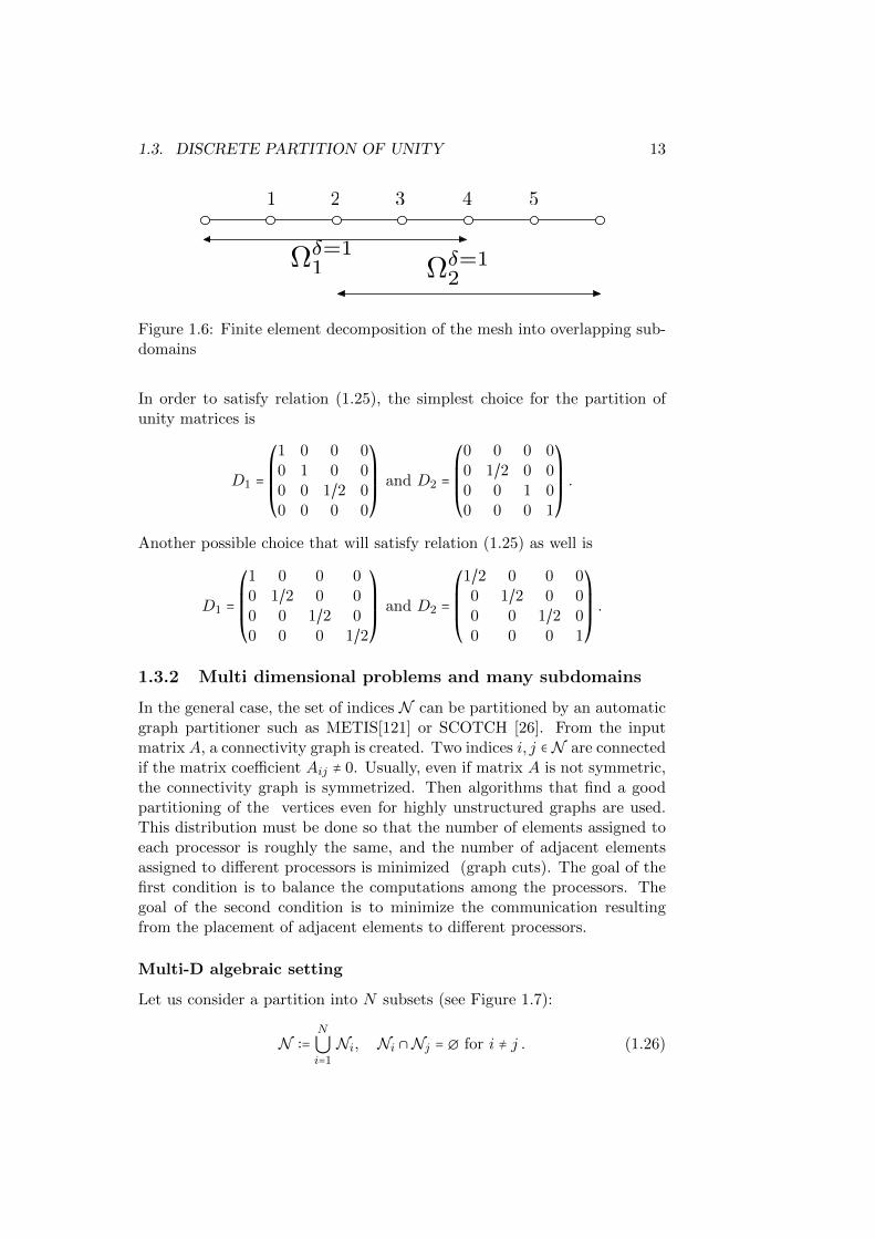
1.5. CONVERGENCE ANALYSIS 17
L1l2 L
e11 e1
2
e21
e22
e31
0
x
δ
e02
Figure 1.9: Convergence of the Schwarz method
Thus, we have
en+12 (L1) = en+1
1 (l2)L −L1
L − l2= en2(L1)
l2L1
L −L1
L − l2.
Let δ ∶= L1 − l2 denote the size of the overlap, we have
en+12 (L1) =
l2l2 + δ
L − l2 − δL − l2
en2(L1) =1 − δ/(L − l2)
1 + δ/l2en2(L1) .
We see that the following quantity is the convergence factor of the algorithm
ρ1 =1 − δ/(L − l2)
1 + δ/l2
It is clear that δ > 0 is a sufficient and necessary condition to have con-vergence. The convergence becomes faster as the ratio of the size of theoverlap over the size of a subdomain is bigger. A geometric illustration ofthe history of the convergence can be found in figure 1.9.
1.5.2 2d case: Fourier analysis for two subdomains
For sake of simplicity we consider the plane R2 decomposed into two half-planes Ω1 = (−∞, δ) × R and Ω2 = (0,∞) × R with an overlap of size δ > 0.

18 CHAPTER 1. SCHWARZ METHODS
We choose as an example a symmetric positive definite problem (η > 0)
(η −∆)(u) = f in R2,
u is bounded at infinity ,
The Jacobi-Schwarz method for this problem is the following iteration
(η −∆)(un+11 ) = f(x, y), (x, y) ∈ Ω1
un+11 (δ, y) = un2(δ, y), y ∈ R
(1.32)
and(η −∆)(un+1
2 ) = f(x, y), (x, y) ∈ Ω2
un+12 (0, y) = un1(0, y), y ∈ R
(1.33)
with the local solutions un+1j , j = 1,2 bounded at infinity.
In order to compute the convergence factor, we introduce the errors
eni ∶= uni − u∣Ωi , i = 1,2.
By linearity, the errors satisfy the above algorithm with f = 0:
(η −∆)(en+11 ) = f(x, y), (x, y) ∈ Ω1
en+11 (δ, y) = en2(δ, y), y ∈ R
(1.34)
and(η −∆)(en+1
2 ) = f(x, y), (x, y) ∈ Ω2
en+12 (0, y) = en1(0, y), y ∈ R
(1.35)
with en+1j bounded at infinity.
By taking the partial Fourier transform of the first line of (1.34) in they direction we get:
(η − ∂2
∂x2+ k2)(en+1
1 (x, k)) = 0 in Ω1.
For a given Fourier variable k, this is an ODE whose solution is sought inthe form
en+11 (x, k) =∑
j
γj(k) exp(λj(k)x).
A simple computation gives
λ1(k) = λ+(k), λ2(k) = λ−(k), with λ±(k) = ±√η + k2.
Therefore we have
en+11 (x, k) = γn+1
+ (k) exp(λ+(k)x) + γn+1− (k) exp(λ−(k)x).

1.6. MORE SOPHISTICATED SCHWARZMETHODS: P.L. LIONS’ ALGORITHM19
Since the solution must be bounded at x = −∞, this implies that γn+1− (k) ≡ 0.
Thus we haveen+1
1 (x, k) = γn+1+ (k) exp(λ+(k)x)
or equivalently, by changing the value of the coefficient γ+,
en+11 (x, k) = γn+1
1 (k) exp(λ+(k)(x − δ))
and similarly, in domain Ω2 we have:
en+12 (x, k) = γn+1
2 (k) exp(λ−(k)x)
with γn+11,2 to be determined. From the interface conditions we get
γn+11 (k) = γn2 (k) exp(λ−(k)δ)
andγn+1
2 (k) = γn1 (k) exp(−λ+(k)δ).Combining these two and denoting λ(k) = λ+(k) = −λ−(k), we get for i = 1,2,
γn+1i (k) = ρ(k;α, δ)2 γn−1
i (k)
with ρ the convergence factor given by:
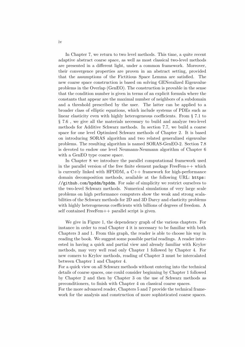
ρ(k;α, δ) = exp(−λ(k)δ), λ(k) =√η + k2. (1.36)
A graphical representation can be found in Figure 1.10 for some values ofthe overlap. This formula deserves a few remarks.
Remark 1.5.1 We have the following properties:
• For all k ∈ R, ρ(k) < exp(−√η δ) < 1 so that γni (k)→ 0 uniformly as ngoes to infinity.
• ρ→ 0 as k tends to infinity, high frequency modes of the error convergevery fast.
• When there is no overlap (δ = 0), ρ = 1 and there is stagnation of themethod.
1.6 More sophisticated Schwarz methods: P.L. Li-ons’ Algorithm
During the last decades, more sophisticated Schwarz methods were designed,namely the optimized Schwarz methods. These methods are based on aclassical domain decomposition, but they use more effective transmission

20 CHAPTER 1. SCHWARZ METHODS
k
ρ
exp sqrt.1k^ 2 , exp 0.5sqrt.1k^ 2 , k from 0 to 7
Input in terpre ta tion :
p lotexp 0.1 k 2 exp 0.5 0.1 k 2 k 0 to 7
Plo t:
1 2 3 4 5 6 7
0.2
0.4
0.6
0.8
k 20.1
0.5 k 20.1
Genera ted by Wolfram |Alpha (www.wolfram alpha.com ) on October 26 , 2011 from Cham paign, IL.© Wolfram Alpha LLC—A Wolfram Research Company
1
Figure 1.10: Convergence rate of the Schwarz method for η = .1, δ = 0.5 (redcurve) or δ = 1 (blue curve).
1 2n1
n21 2n1n2
Figure 1.11: Outward normals for overlapping and non overlapping subdo-mains for P.L. Lions’ algorithm.
1.7. SCHWARZ METHODS USING FREEFEM++ 21
conditions than the classical Dirichlet conditions at the interfaces betweensubdomains. The first more effective transmission conditions were first in-troduced by P.L. Lions’ [129]. For elliptic problems, we have seen thatSchwarz algorithms work only for overlapping domain decompositions andtheir performance in terms of iterations counts depends on the width ofthe overlap. The algorithm introduced by P.L. Lions [129] can be applied toboth overlapping and non overlapping subdomains. It is based on improvingSchwarz methods by replacing the Dirichlet interface conditions by Robininterface conditions.
Let α be a positive number, the modified algorithm reads
−∆(un+11 ) = f in Ω1,
un+11 = 0 on ∂Ω1 ∩ ∂Ω,
( ∂
∂n1+ α) (un+1
1 ) = ( ∂
∂n1+ α) (un2) on ∂Ω1 ∩Ω2 ,
(1.37)
and
−∆(un+12 ) = f in Ω2,
un+12 = 0 on ∂Ω2 ∩ ∂Ω
( ∂
∂n2+ α) (un+1
2 ) = ( ∂
∂n2+ α) (un1) on ∂Ω2 ∩Ω1
(1.38)
where n1 and n2 are the outward normals on the boundary of the subdo-mains, see Figure 1.11.
This algorithm was extended to Helmholtz problem by Despres [45]. Itis also possible to consider other interface conditions than Robin conditionsand optimize their choice with respect to the convergence factor. All theseideas will be presented in detail in Chapter 2.
1.7 Schwarz methods using FreeFem++
The aim of this part is to illustrate numerically the previously definedSchwarz methods applied to second order elliptic boundary value problems(e.g Laplace equation and elasticity). In order to do this we will use thefree finite element software FreeFem++ [108] developed at the LaboratoireJacques-Louis Lions at Universite Pierre et Marie Curie (Paris 6).
1.7.1 A very short introduction to FreeFem++
FreeFem++ allows a very simple and natural way to solve a great varietyof variational problems by finite element type methods including Discon-tinuous Galerkin (DG) discretizations. It is also possible to have access tothe underlying linear algebra such as the stiffness or mass matrices. In this
22 CHAPTER 1. SCHWARZ METHODS
section we will provide only a minimal number of elements of this software,necessary for the understanding of the programs in the next section, see alsohttp://www.cmap.polytechnique.fr/spip.php?article239. A very de-tailed documentation of FreeFem++ is available on the official websitehttp://www.freefem.org/ff++, at the following addresshttp://www.freefem.org/ff++/ftp/freefem++doc.pdf . The standardimplementation includes tons of very useful examples that make a tuto-rial by themselves. It is also possible to use the integrated environ-ment FreeFem++-cs [124] which provides an intuitive graphical interfaceto FreeFem++ users.
To start with, suppose we want to solve a very simple homogeneousDirichlet boundary value problem for a Laplacian defined on a unit squareΩ =]0,1[2:
−∆u = f in Ωu = 0 on ∂Ω
(1.39)
The variational formulation of this problem reads:
Find u ∈H10(Ω) ∶= w ∈H1(Ω) ∶ w = 0 on ∂Ω such that
∫Ω∇u.∇vdx − ∫
Ωf v dx = 0,∀v ∈H1
0(Ω) .
A feature of FreeFem++ is to penalize Dirichlet boundary conditions. Theabove variational formulation is first replaced by
Find u ∈H1(Ω) such that
∫Ω∇u.∇vdx − ∫
Ωfv dx = 0,∀v ∈H1(Ω) .
Then the finite element approximation leads to a system of the type
M
∑j=1
Aijuj − Fj = 0, i = 1, ...,M, Aij = ∫Ω∇φi.∇φjdx,Fi = ∫
Ωφi dx
where (φi)1≤i≤M are the finite element functions. Note that the discretizedsystem corresponds to a Neumann problem. Dirichlet conditions of the typeu = g are then implemented by penalty, namely by setting
Aii = 1030, Fi = 1030 ⋅ gi
if i is a boundary degree of freedom. The penalty number 1030 is calledTGV1 and it is possible to change this value. The keyword on imposes theDirichlet boundary condition through this penalty term.
1Tres Grande Valeur (Terrifically Great Value) = Very big value in French

1.7. SCHWARZ METHODS USING FREEFEM++ 23
Ω
Γ3
Γ2
Γ1
Γ4
Figure 1.12: Numbering of square borders in FreeFem++
The following FreeFem++ script is solving this problem in a few lines.The text after // symbols are comments ignored by the FreeFem++ lan-guage. Each new variable must be declared with its type (here int designsintegers).
3 // Number of mesh points in x and y directionsint Nbnoeuds=10;
Listing 1.1: ./FreefemCommon/survival.edp
The function square returns a structured mesh of the square: the first twoarguments are the number of mesh points according to x and y directionsand the third one is a parametrization of Ω for x and y varying between 0and 1 (here it is the identity). The sides of the square are labeled from 1 to4 in trigonometrical sense (see Figure 1.12).
//Mesh definitionmesh Th=square(Nbnoeuds,Nbnoeuds,[x,y]);
Listing 1.2: ./FreefemCommon/survival.edp
We define the function representing the right-hand side using the keywordfunc
// Functions of x and y14 func f=x∗y;
func g=1.;
Listing 1.3: ./FreefemCommon/survival.edp

24 CHAPTER 1. SCHWARZ METHODS
and the P1 finite element space Vh over the mesh Th using the keywordfespace
// Finite element space on the mesh Thfespace Vh(Th,P1);//uh and vh are of type Vh
22 Vh uh,vh;
Listing 1.4: ./FreefemCommon/survival.edp
The functions uh and vh belong to the P1 finite element space Vh which isan approximation to H1(Ω). Note here that if one wants to use P2 insteadP1 finite elements, it is enough to replace P1 by P2 in the definition of Vh.
26 // variational problem definitionproblem heat(uh,vh,solver=LU)=
int2d(Th)(dx(uh)∗dx(vh)+dy(uh)∗dy(vh))−int2d(Th)(f∗vh)
30 +on(1,2,3,4,uh=0);
Listing 1.5: ./FreefemCommon/survival.edp
The keyword problem allows the definition of a variational problem, herecalled heat which can be expressed mathematically as:Find uh ∈ Vh such that
∫Ω∇uh.∇vhdx − ∫
Ωfvhdx = 0,∀vh ∈ Vh .
Afterwards, for the Dirichlet boundary condition the penalization isimposed using TGV which is usually is equal to 1030.
Note that keyword problem defines problem (1.39) without solving it. Theparameter solver sets the method that will be used to solve the resultinglinear system, here a Gauss factorization. In order to effectively solve thefinite element problem, we need the command
34 //Solving the problemheat;// Plotting the resultplot(uh,wait=1);
Listing 1.6: ./FreefemCommon/survival.edp

1.7. SCHWARZ METHODS USING FREEFEM++ 25
The FreeFem++ script can be saved with your favorite text editor (e.g.under the name heat.edp). In order to execute the script FreeFem++, itis enough to write the shell command FreeFem++ heat.edp. The resultwill be displayed in a graphic window.
One can easily modify the script in order to solve the same kind of problemsbut with mixed Neumann and Fourier boundary conditions such as
⎧⎪⎪⎪⎪⎪⎪⎪⎨⎪⎪⎪⎪⎪⎪⎪⎩
−∆u + u = f in Ω∂u
∂n= 0 on Γ1
u = 0 on Γ2∂u∂n + αu = g on Γ3 ∪ Γ4.
(1.40)
where f and g are arbitrary functions and α a positive real.The new variational formulation consists in determining uh ∈ Vh such that
∫Ω∇uh.∇vhdx + ∫
Γ3∪Γ4
αuhvh − ∫Γ3∪Γ4
gvh − ∫Ωfvhdx = 0,
for all vh ∈ Vh. Here again the Dirichlet boundary condition will bepenalized. The FreeFem++ definition of the problem reads:
// Changing boundary conditions to Neumann or Robin42 real alpha =1.;
problem heatRobin(uh,vh)=int2d(Th)(dx(uh)∗dx(vh)+dy(uh)∗dy(vh))+int1d(Th,3,4)(alpha∗uh∗vh)
46 −int1d(Th,3,4)(g∗vh)−int2d(Th)(f∗vh)+on(2,uh=0);
Listing 1.7: ./FreefemCommon/survival.edp
In the variational formulation of (1.40) the extra boundary integralon Γ3 ∪ Γ4 is defined by the keyword int1d(Th,3,4)(function to
integrate).
The keyword varf allows the definition of a variational formulation
// Using linear algebra packagevarf varheatRobin(uh,vh)=
54 int2d(Th)(dx(uh)∗dx(vh)+dy(uh)∗dy(vh))+int1d(Th,3,4)(alpha∗uh∗vh)−int1d(Th,3,4)(g∗vh)−int2d(Th)(f∗vh)
58 +on(2,uh=0);
26 CHAPTER 1. SCHWARZ METHODS
Listing 1.8: ./FreefemCommon/survival.edp
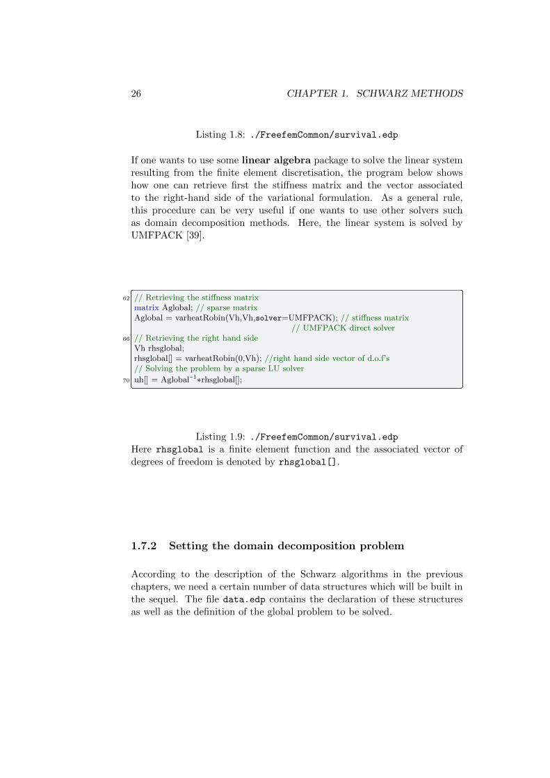
If one wants to use some linear algebra package to solve the linear systemresulting from the finite element discretisation, the program below showshow one can retrieve first the stiffness matrix and the vector associatedto the right-hand side of the variational formulation. As a general rule,this procedure can be very useful if one wants to use other solvers suchas domain decomposition methods. Here, the linear system is solved byUMFPACK [39].
62 // Retrieving the stiffness matrixmatrix Aglobal; // sparse matrixAglobal = varheatRobin(Vh,Vh,solver=UMFPACK); // stiffness matrix
// UMFPACK direct solver66 // Retrieving the right hand side
Vh rhsglobal;rhsglobal[] = varheatRobin(0,Vh); //right hand side vector of d.o.f’s// Solving the problem by a sparse LU solver
70 uh[] = Aglobal−1∗rhsglobal[];
Listing 1.9: ./FreefemCommon/survival.edpHere rhsglobal is a finite element function and the associated vector ofdegrees of freedom is denoted by rhsglobal[].
1.7.2 Setting the domain decomposition problem
According to the description of the Schwarz algorithms in the previouschapters, we need a certain number of data structures which will be built inthe sequel. The file data.edp contains the declaration of these structuresas well as the definition of the global problem to be solved.

1.7. SCHWARZ METHODS USING FREEFEM++ 27
1 load ”metis” // mesh partitionerload ”medit” // OpenGL−based scientific visualization softwareint nn=2,mm=2; // number of the domains in each directionint npart= nn∗mm; // total number of domains
5 int nloc = 20; // local no of dof per domain in one directionbool withmetis = 1; // =1 (Metis decomp) =0 (uniform decomp)int sizeovr = 1; // size of the geometric overlap between subdomains, algebraic ⤸
Ç overlap is sizeovr+1real allong = real(nn)/real(mm); // aspect ratio of the global domain
9 // Mesh of a rectangular domainmesh Th=square(nn∗nloc,mm∗nloc,[x∗allong,y]);// radial mesh ⤸
Ç [(1.+x∗allong)∗cos(pi∗y),(1.+x∗allong)∗sin(pi∗y)]);//fespace Vh(Th,P1);fespace Ph(Th,P0);
13 Ph part; // piecewise constant functionint[int] lpart(Ph.ndof); // giving the decomposition// Domain decomposition data structuresmesh[int] aTh(npart); // sequence of subdomain meshes
17 matrix[int] Rih(npart); // local restriction operatorsmatrix[int] Dih(npart); // partition of unity operatorsint[int] Ndeg(npart); // number of dof for each meshreal[int] AreaThi(npart); // area of each subdomain
21 matrix[int] aA(npart),aN(npart); // local matricesVh[int] Z(npart); // coarse space, see Chapter 3// Definition of the problem to solve// Delta (u) = f, u = 1 on the global boundary
25 //int[int] chlab=[1,1 ,2,1 ,3,1 ,4,1 ];//Th=change(Th,refe=chlab); // all label borders are set to onemacro Grad(u) [dx(u),dy(u)] // EOMfunc f = 1; // right hand side
29 func g = 0 ; // Dirichlet datafunc kappa = 1.; // viscosityfunc eta = 0;Vh rhsglobal,uglob; // rhs and solution of the global problem
33 varf vaglobal(u,v) = int2d(Th)(eta∗u∗v+kappa∗Grad(u)’∗Grad(v))+on(1,u=g) + int2d(Th)(f∗v);
matrix Aglobal;// Iterative solver parameters
37 real tol=1e−6; // tolerance for the iterative methodint maxit=300; // maximum number of iterations
Listing 1.10: ./FreefemCommon/data.edp
Afterwards we have to define a piecewise constant function part whichtakes integer values. The isovalues of this function implicitly defines a nonoverlapping partition of the domain. We have a coloring of the subdomains.
Suppose we want a decomposition of a rectangle Ω into nn×mm domains withapproximately nloc points in one direction, or a more general partitioningmethod, using for example METIS [121] or SCOTCH [26]. In order toperform one of these decompositions, we make use of one of the routines
28 CHAPTER 1. SCHWARZ METHODS
IsoValue-0.1578950.07894740.2368420.3947370.5526320.7105260.8684211.026321.184211.342111.51.657891.815791.973682.131582.289472.447372.605262.763163.15789
uniform decompositionIsoValue-0.1578950.07894740.2368420.3947370.5526320.7105260.8684211.026321.184211.342111.51.657891.815791.973682.131582.289472.447372.605262.763163.15789
Metis decomposition
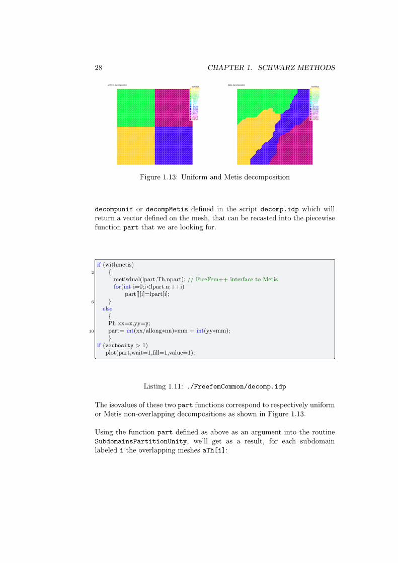
Figure 1.13: Uniform and Metis decomposition
decompunif or decompMetis defined in the script decomp.idp which willreturn a vector defined on the mesh, that can be recasted into the piecewisefunction part that we are looking for.
if (withmetis)2
metisdual(lpart,Th,npart); // FreeFem++ interface to Metisfor(int i=0;i<lpart.n;++i)
part[][i]=lpart[i];6
elsePh xx=x,yy=y;
10 part= int(xx/allong∗nn)∗mm + int(yy∗mm);
if (verbosity > 1)plot(part,wait=1,fill=1,value=1);
Listing 1.11: ./FreefemCommon/decomp.idp
The isovalues of these two part functions correspond to respectively uniformor Metis non-overlapping decompositions as shown in Figure 1.13.
Using the function part defined as above as an argument into the routineSubdomainsPartitionUnity, we’ll get as a result, for each subdomainlabeled i the overlapping meshes aTh[i]:

1.7. SCHWARZ METHODS USING FREEFEM++ 29
func bool SubdomainsPartitionUnity(mesh & Th, real[int] & partdof, int ⤸Ç sizeoverlaps, mesh[int] & aTh, matrix[int] & Rih, matrix[int] & Dih, int[int] ⤸Ç & Ndeg, real[int] & AreaThi)
33 int npart=partdof.max+1;
mesh Thi=Th; // freefem’s trick, formal definitionfespace Vhi(Thi,P1); // freefem’s trick, formal definitionVhi[int] pun(npart); // local fem functions
37 Vh sun=0, unssd=0;Ph part;part[]=partdof;for(int i=0;i<npart;++i)
41 Ph suppi= abs(part−i)<0.1; // boolean 1 in the subdomain 0 elswhereAddLayers(Th,suppi[],sizeoverlaps,unssd[]); // ovr partitions by adding layersThi=aTh[i]=trunc(Th,suppi>0,label=10,split=1);// ovr mesh interfaces label ⤸
Ç 1045 Rih[i]=interpolate(Vhi,Vh,inside=1); // Restriction operator : Vh −> Vhi
pun[i][]=Rih[i]∗unssd[];pun[i][] = 1.;// a garder par la suitesun[] += Rih[i]’∗pun[i][];
49 Ndeg[i] = Vhi.ndof;AreaThi[i] = int2d(Thi)(1.);
for(int i=0;i<npart;++i)
53 Thi=aTh[i];pun[i]= pun[i]/sun;Dih[i]=pun[i][]; //diagonal matrix built from a vector
57 if(verbosity > 1)plot(pun[i],wait=1,value=1,fill=1,dim=3);
return true;
61
Listing 1.12: ./FreefemCommon/createPartition.idp
Note that in the CreatePartition.idp script, the function AddLayers iscalled:
30 CHAPTER 1. SCHWARZ METHODS
func bool AddLayers(mesh & Th,real[int] &ssd,int n,real[int] &unssd)3
// build a continuous function uussd (P1) and modifies ssd :// IN: ssd in the caracteristics function on the input subdomain.// OUT: ssd is a boolean function, unssd is a smooth function
7 // ssd = 1 if unssd >0; add n layer of element and unssd = 0 ouside of this layerPh s;assert(ssd.n==Ph.ndof);assert(unssd.n==Vh.ndof);
11 unssd=0;s[]= ssd;Vh u;varf vM(uu,v)=int2d(Th,qforder=1)(uu∗v/area);
15 matrix M=vM(Ph,Vh);for(int i=0;i<n;++i)
u[]= M∗s[];19 u = u>.1;
unssd+= u[];s[]= M’∗u[];s = s >0.1;
23 unssd /= (n);u[]=unssd;ssd=s[];
27 return true;
Listing 1.13: ./FreefemCommon/createPartition.idpThese last two functions are tricky. The reader does not need to understandtheir behavior in order to use them. They are given here for sake ofcompleteness. The restriction/interpolation operators Rih[i] from thelocal finite element space Vh[i] to the global one Vh and the diagonal localmatrices Dih[i] are thus created.
Afterwards one needs to build the overlapping decomposition and theassociated algebraic partition of unity, see equation (1.25). Programtestdecomp.edp (see below) shows such an example by checking that thepartition of unity is correct.
1.7. SCHWARZ METHODS USING FREEFEM++ 31
load ”medit”
3 verbosity=2;include ”dataGENEO.edp”include ”decomp.idp”include ”createPartition.idp”
7 SubdomainsPartitionUnity(Th,part[],sizeovr,aTh,Rih,Dih,Ndeg,AreaThi);// check the partition of unityVh sum=0,fctone=1;for(int i=0; i < npart;i++)
11 Vh localone;
real[int] bi = Rih[i]∗fctone[]; // restriction to the local domainreal[int] di = Dih[i]∗bi;
15 localone[] = Rih[i]’∗di;sum[] +=localone[] ;plot(localone,fill=1,value=1, dim=3,wait=1);
19 plot(sum,fill=1,value=1, dim=3,wait=1);
Listing 1.14: ./FreefemCommon/testdecomp.edp
Suppose we want to do now the same thing in a three-dimensionalcase.
1 load ”msh3”func mesh3 Cube(int[int] & NN,real[int,int] &BB ,int[int,int] & L)// basic functions to build regular mesh of a cube// int[int] NN=[nx,ny,nz]; the number of seg in the 3 direction
5 // real [int,int] BB=[[xmin,xmax],[ymin,ymax],[zmin,zmax]]; bounding bax// int [int,int] L=[[1,2],[3,4],[5,6]]; label of the 6 faces left,right, front, back, down, up
// first build the 6 faces of the cube.9 real x0=BB(0,0),x1=BB(0,1);
real y0=BB(1,0),y1=BB(1,1);real z0=BB(2,0),z1=BB(2,1);int nx=NN[0],ny=NN[1],nz=NN[2];
13 mesh Thx = square(nx,ny,[x0+(x1−x0)∗x,y0+(y1−y0)∗y]);
int[int] rup=[0,L(2,1)], rdown=[0,L(2,0)],rmid=[1,L(1,0), 2,L(0,1), 3, L(1,1), 4, L(0,0) ];
17 mesh3 Th=buildlayers(Thx,nz, zbound=[z0,z1],labelmid=rmid, labelup = rup, labeldown = rdown);
return Th;
Listing 1.15: ./FreefemCommon/cube.idp
We would like to build a cube or a parallelepiped defined by calling thefunction Cube defined in the script cube.idp and then to split it intoseveral domains. Again we need a certain number of data structures which
32 CHAPTER 1. SCHWARZ METHODS
will be declared in the file data3d.edp
load ”metis”load ”medit”int nn=2,mm=2,ll=2; // number of the domains in each direction
4 int npart= nn∗mm∗ll; // total number of domainsint nloc = 11; // local no of dof per domain in one directionbool withmetis = 1; // =1 (Metis decomp) =0 (uniform decomp)int sizeovr = 2; // size of the overlap
8 real allongx, allongz;allongx = real(nn)/real(mm);allongz = real(ll)/real(mm);// Build the mesh
12 include ”cube.idp”int[int] NN=[nn∗nloc,mm∗nloc,ll∗nloc];real [int,int] BB=[[0,allongx],[0,1],[0,allongz]]; // bounding boxint [int,int] L=[[1,1],[1,1],[1,1]]; // the label of the 6 faces
16 mesh3 Th=Cube(NN,BB,L); // left,right,front, back, down, rightfespace Vh(Th,P1);fespace Ph(Th,P0);Ph part; // piecewise constant function
20 int[int] lpart(Ph.ndof); // giving the decomposition// domain decomposition data structuresmesh3[int] aTh(npart); // sequence of ovr. meshesmatrix[int] Rih(npart); // local restriction operators
24 matrix[int] Dih(npart); // partition of unity operatorsint[int] Ndeg(npart); // number of dof for each meshreal[int] VolumeThi(npart); // volume of each subdomainmatrix[int] aA(npart); // local Dirichlet matrices
28 Vh[int] Z(npart); // coarse space// Definition of the problem to solve// Delta (u) = f, u = 1 on the global boundaryVh intern;
32 intern = (x>0) && (x<allongx) && (y>0) && (y<1) && (z>0) && (z<allongz);Vh bord = 1−intern;macro Grad(u) [dx(u),dy(u),dz(u)] // EOMfunc f = 1; // right hand side
36 func g = 1; // Dirichlet dataVh rhsglobal,uglob; // rhs and solution of the global problemvarf vaglobal(u,v) = int3d(Th)(Grad(u)’∗Grad(v))
+on(1,u=g) + int3d(Th)(f∗v);40 matrix Aglobal;
// Iterative solverreal tol=1e−10; // tolerance for the iterative methodint maxit=200; // maximum number of iterations
Listing 1.16: ./FreefemCommon/data3d.edp
Then we have to define a piecewise constant function part which takes inte-ger values. The isovalues of this function implicitly defines a non overlappingpartition of the domain. Suppose we want a decomposition of a rectangle Ω
1.7. SCHWARZ METHODS USING FREEFEM++ 33
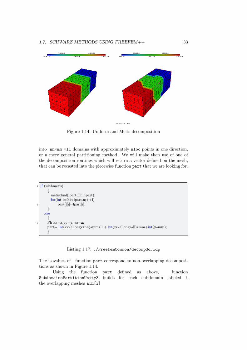
Figure 1.14: Uniform and Metis decomposition
into nn×mm ×ll domains with approximately nloc points in one direction,or a more general partitioning method. We will make then use of one ofthe decomposition routines which will return a vector defined on the mesh,that can be recasted into the piecewise function part that we are looking for.
1 if (withmetis)
metisdual(lpart,Th,npart);for(int i=0;i<lpart.n;++i)
5 part[][i]=lpart[i];
else
9 Ph xx=x,yy=y, zz=z;part= int(xx/allongx∗nn)∗mm∗ll + int(zz/allongz∗ll)∗mm+int(y∗mm);
Listing 1.17: ./FreefemCommon/decomp3d.idp
The isovalues of function part correspond to non-overlapping decomposi-tions as shown in Figure 1.14.
Using the function part defined as above, functionSubdomainsPartitionUnity3 builds for each subdomain labeled i
the overlapping meshes aTh[i]

34 CHAPTER 1. SCHWARZ METHODS
31 func bool SubdomainsPartitionUnity3(mesh3 & Th, real[int] & partdof, int ⤸Ç sizeoverlaps, mesh3[int] & aTh, matrix[int] & Rih, matrix[int] & Dih, int[int] ⤸Ç & Ndeg, real[int] & VolumeThi)
int npart=partdof.max+1;mesh3 Thi=Th; // freefem’s trick, formal definition
35 fespace Vhi(Thi,P1); // freefem’s trick, formal definitionVhi[int] pun(npart); // local fem functionsVh sun=0, unssd=0;Ph part;
39 part[]=partdof;for(int i=0;i<npart;++i)
// boolean function 1 in the subdomain 0 elswhere43 Ph suppi= abs(part−i)<0.1;
AddLayers3(Th,suppi[],sizeoverlaps,unssd[]); // overlapping partitions by ⤸Ç adding layers
Thi=aTh[i]=trunc(Th,suppi>0,label=10,split=1); // overlapping mesh, ⤸Ç interfaces have label 10
Rih[i]=interpolate(Vhi,Vh,inside=1); // Restriction operator : Vh −> Vhi47 pun[i][]=Rih[i]∗unssd[];
sun[] += Rih[i]’∗pun[i][];Ndeg[i] = Vhi.ndof;VolumeThi[i] = int3d(Thi)(1.);
51 for(int i=0;i<npart;++i)
Thi=aTh[i];55 pun[i]= pun[i]/sun;
Dih[i]=pun[i][];//diagonal matrix built from a vector
return true;59
Listing 1.18: ./FreefemCommon/createPartition3d.idp
by making use of the function AddLayers3 in the CreatePartition3d.idp.
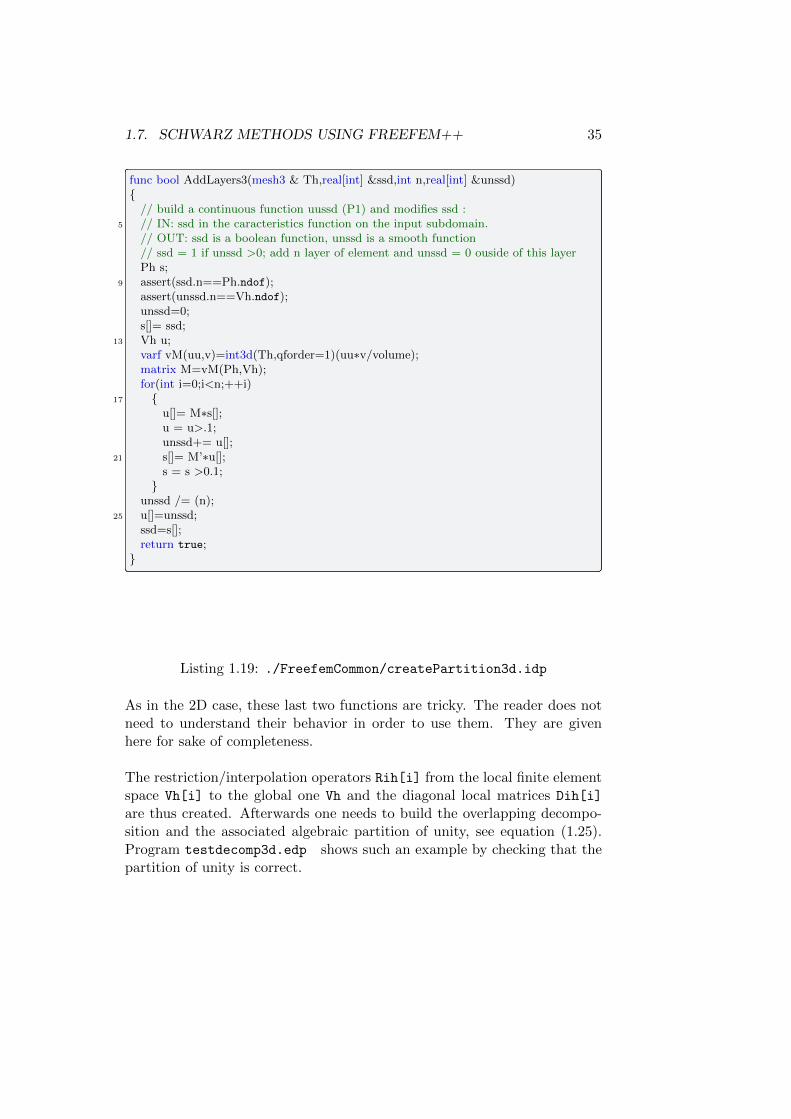
1.7. SCHWARZ METHODS USING FREEFEM++ 35
func bool AddLayers3(mesh3 & Th,real[int] &ssd,int n,real[int] &unssd)
// build a continuous function uussd (P1) and modifies ssd :5 // IN: ssd in the caracteristics function on the input subdomain.
// OUT: ssd is a boolean function, unssd is a smooth function// ssd = 1 if unssd >0; add n layer of element and unssd = 0 ouside of this layerPh s;
9 assert(ssd.n==Ph.ndof);assert(unssd.n==Vh.ndof);unssd=0;s[]= ssd;
13 Vh u;varf vM(uu,v)=int3d(Th,qforder=1)(uu∗v/volume);matrix M=vM(Ph,Vh);for(int i=0;i<n;++i)
17 u[]= M∗s[];u = u>.1;unssd+= u[];
21 s[]= M’∗u[];s = s >0.1;
unssd /= (n);
25 u[]=unssd;ssd=s[];return true;
Listing 1.19: ./FreefemCommon/createPartition3d.idp
As in the 2D case, these last two functions are tricky. The reader does notneed to understand their behavior in order to use them. They are givenhere for sake of completeness.
The restriction/interpolation operators Rih[i] from the local finite elementspace Vh[i] to the global one Vh and the diagonal local matrices Dih[i]
are thus created. Afterwards one needs to build the overlapping decompo-sition and the associated algebraic partition of unity, see equation (1.25).Program testdecomp3d.edp shows such an example by checking that thepartition of unity is correct.
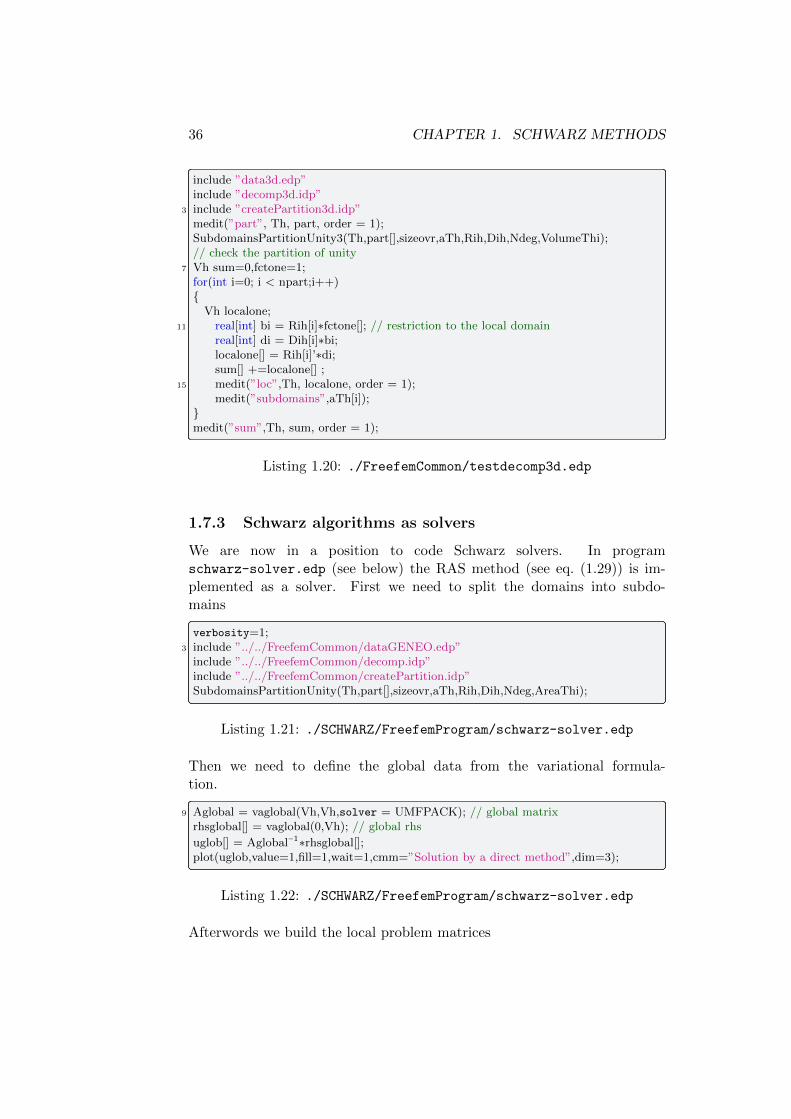
36 CHAPTER 1. SCHWARZ METHODS
include ”data3d.edp”include ”decomp3d.idp”
3 include ”createPartition3d.idp”medit(”part”, Th, part, order = 1);SubdomainsPartitionUnity3(Th,part[],sizeovr,aTh,Rih,Dih,Ndeg,VolumeThi);// check the partition of unity
7 Vh sum=0,fctone=1;for(int i=0; i < npart;i++)
Vh localone;11 real[int] bi = Rih[i]∗fctone[]; // restriction to the local domain
real[int] di = Dih[i]∗bi;localone[] = Rih[i]’∗di;sum[] +=localone[] ;
15 medit(”loc”,Th, localone, order = 1);medit(”subdomains”,aTh[i]);
medit(”sum”,Th, sum, order = 1);
Listing 1.20: ./FreefemCommon/testdecomp3d.edp
1.7.3 Schwarz algorithms as solvers
We are now in a position to code Schwarz solvers. In programschwarz-solver.edp (see below) the RAS method (see eq. (1.29)) is im-plemented as a solver. First we need to split the domains into subdo-mains
verbosity=1;3 include ”../../FreefemCommon/dataGENEO.edp”
include ”../../FreefemCommon/decomp.idp”include ”../../FreefemCommon/createPartition.idp”SubdomainsPartitionUnity(Th,part[],sizeovr,aTh,Rih,Dih,Ndeg,AreaThi);
Listing 1.21: ./SCHWARZ/FreefemProgram/schwarz-solver.edp
Then we need to define the global data from the variational formula-tion.
9 Aglobal = vaglobal(Vh,Vh,solver = UMFPACK); // global matrixrhsglobal[] = vaglobal(0,Vh); // global rhs
uglob[] = Aglobal−1∗rhsglobal[];plot(uglob,value=1,fill=1,wait=1,cmm=”Solution by a direct method”,dim=3);
Listing 1.22: ./SCHWARZ/FreefemProgram/schwarz-solver.edp
Afterwords we build the local problem matrices

1.7. SCHWARZ METHODS USING FREEFEM++ 37
for(int i = 0;i<npart;++i)
17 cout << ” Domain :” << i << ”/” << npart << endl;matrix aT = Aglobal∗Rih[i]’;aA[i] = Rih[i]∗aT;set(aA[i],solver = UMFPACK);// direct solvers
21
Listing 1.23: ./SCHWARZ/FreefemProgram/schwarz-solver.edp
and finally the Schwarz iteration
ofstream filei(”Conv.m”);25 Vh un = 0; // initial guess
Vh rn = rhsglobal;for(int iter = 0;iter<maxit;++iter)
29 real err = 0, res;Vh er = 0;for(int i = 0;i<npart;++i)
33 real[int] bi = Rih[i]∗rn[]; // restriction to the local domain
real[int] ui = aA[i] −1∗ bi; // local solvebi = Dih[i]∗ui;// bi = ui; // uncomment this line to test the ASM method as a solver
37 er[] += Rih[i]’∗bi;
un[] += er[]; // build new iteratern[] = Aglobal∗un[]; // computes global residual
41 rn[] = rn[] − rhsglobal[];rn[] ∗= −1;err = sqrt(er[]’∗er[]);res = sqrt(rn[]’∗rn[]);
45 cout << ”Iteration: ” << iter << ” Correction = ” << err << ” Residual = ” ⤸Ç << res << endl;
plot(un,wait=1,value=1,fill=1,dim=3,cmm=”Approximate solution at step ” + ⤸Ç iter);
int j = iter+1;// Store the error and the residual in Matlab/Scilab/Octave form
49 filei << ”Convhist(”+j+”,:)=[” << err << ” ” << res <<”];” << endl;if(err < tol) break;
plot(un,wait=1,value=1,fill=1,dim=3,cmm=”Final solution”);
Listing 1.24: ./SCHWARZ/FreefemProgram/schwarz-solver.edp
The convergence history of the algorithm is stored in a Matlab file (alsocompatible with Scilab or Octave) Conv.m, under the form of a two-columnmatrix containing the error evolution as well as the residual one.

38 CHAPTER 1. SCHWARZ METHODS
0 10 20 30 40 50 6010 6
10 5
10 4
10 3
10 2
10 1
100
101
102
overlap=2overlap=5overlap=10
Figure 1.15: Solution and RAS convergence as a solver for different overlaps
The result of tracing the evolution of the error is shown in Figure 1.15 whereone can see the convergence history of the RAS solver for different values ofthe overlapping parameter.
Remark 1.7.1 Previous tests have shown a very easy use of the RAS iter-ative algorithm and some straightforward conclusions from this.
• The convergence of RAS, not very fast even in a simple configurationof 4 subdomains, improves when the overlap is getting bigger.
• Note that it is very easy to test the ASM method, see eq. (1.30), whenused as a solver. It is sufficient to uncomment the line bi = ui;.
• Running the program shows that the ASM does not converge. For thisreason, the ASM method is always used a preconditioner for a Krylovmethod such as CG, GMRES or BiCGSTAB, see chapter 3.
• In the the three-dimensional case the only part that changes is thedecomposition into subdomains. The other parts of the algorithm areidentical.
include ”../../FreefemCommon/data3d.edp”include ”../../FreefemCommon/decomp3d.idp”
4 include ”../../FreefemCommon/createPartition3d.idp”SubdomainsPartitionUnity3(Th,part[],sizeovr,aTh,Rih,Dih,Ndeg,VolumeThi);
Listing 1.25: ./SCHWARZ/FreefemProgram/schwarz-solver3d.edp
1.7.4 Systems of PDEs: the example of linear elasticity
Suppose we want to solve now another kind of problem, such a linear elas-ticity. A few changes will be necessary.

1.7. SCHWARZ METHODS USING FREEFEM++ 39
load ”metis”2 load ”medit”
int nn=3,mm=3; // number of the domains in each directionint npart= nn∗mm; // total number of domainsint nloc = 20; // local no of dof per domain in one direction
6 bool withmetis = 1; // =1 (Metis decomp) =0 (uniform decomp)int sizeovr = 2; // size of the overlapreal allong = real(nn)/real(mm); // aspect ratio of the global domainfunc E = 2∗10ˆ11; // Young modulus ans Poisson ratio
10 func sigma = 0.3;func lambda = E∗sigma/((1+sigma)∗(1−2∗sigma)); // Lame coefficientsfunc mu = E/(2∗(1+sigma));real sqrt2=sqrt(2.);
14 func eta = 1.0e−6;// Mesh of a rectangular domainmesh Th=square(nn∗nloc,mm∗nloc,[x∗allong,y]);fespace Vh(Th,[P1,P1]); // vector fem space
18 fespace Uh(Th,P1); // scalar fem spacefespace Ph(Th,P0);Ph part; // piecewise constant functionint[int] lpart(Ph.ndof); // giving the decomposition
22 // Domain decomposition data structuresmesh[int] aTh(npart); // sequence of ovr. meshesmatrix[int] Rih(npart); // local restriction operatorsmatrix[int] Dih(npart); // partition of unity operators
26 int[int] Ndeg(npart); // number of dof for each meshreal[int] AreaThi(npart); // area of each subdomainmatrix[int] aA(npart); // local Dirichlet matrices// Definition of the problem to solve
30 int[int] chlab=[1,11 ,2,2 ,3,33 ,4,1 ]; //Dirichlet conditions for label = 1Th=change(Th,refe=chlab);macro Grad(u) [dx(u),dy(u)] // EOMmacro epsilon(u,v) [dx(u),dy(v),(dy(u)+dx(v))/sqrt2] // EOM
34 macro div(u,v) ( dx(u)+dy(v) ) // EOMfunc uboundary = (0.25 − (y−0.5)ˆ2);varf vaBC([u,v],[uu,vv]) = on(1, u = uboundary, v=0) + on(11, u = 0, v=0) + ⤸
Ç on(33, u=0,v=0);// global problem
38 Vh [rhsglobal,rrhsglobal], [uglob,uuglob];macro Elasticity(u,v,uu,vv) eta∗(u∗uu+v∗vv) + ⤸
Ç lambda∗(div(u,v)∗div(uu,vv))+2.∗mu∗( epsilon(u,v)’∗epsilon(uu,vv) ) // ⤸Ç EOM
varf vaglobal([u,v],[uu,vv]) = int2d(Th)(Elasticity(u,v,uu,vv)) + vaBC; // ⤸Ç on(1,u=uboundary,v=0)
matrix Aglobal;42 // Iterative solver parameters
real tol=1e−6; // tolerance for the iterative methodint maxit=200; // maximum number of iterations
Listing 1.26: ./FreefemCommon/dataElast.edp
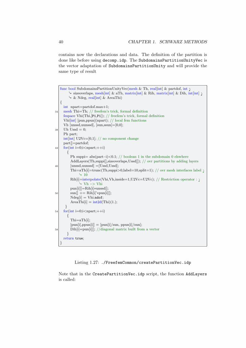
40 CHAPTER 1. SCHWARZ METHODS
contains now the declarations and data. The definition of the partition isdone like before using decomp.idp. The SubdomainsPartitionUnityVec isthe vector adaptation of SubdomainsPartitionUnity and will provide thesame type of result
func bool SubdomainsPartitionUnityVec(mesh & Th, real[int] & partdof, int ⤸Ç sizeoverlaps, mesh[int] & aTh, matrix[int] & Rih, matrix[int] & Dih, int[int] ⤸Ç & Ndeg, real[int] & AreaThi)
int npart=partdof.max+1;
34 mesh Thi=Th; // freefem’s trick, formal definitionfespace Vhi(Thi,[P1,P1]); // freefem’s trick, formal definitionVhi[int] [pun,ppun](npart); // local fem functionsVh [unssd,uunssd], [sun,ssun]=[0,0];
38 Uh Ussd = 0;Ph part;int[int] U2Vc=[0,1]; // no component changepart[]=partdof;
42 for(int i=0;i<npart;++i)
Ph suppi= abs(part−i)<0.1; // boolean 1 in the subdomain 0 elswhereAddLayers(Th,suppi[],sizeoverlaps,Ussd[]); // ovr partitions by adding layers
46 [unssd,uunssd] =[Ussd,Ussd];Thi=aTh[i]=trunc(Th,suppi>0,label=10,split=1); // ovr mesh interfaces label ⤸
Ç 10Rih[i]=interpolate(Vhi,Vh,inside=1,U2Vc=U2Vc); // Restriction operator : ⤸
Ç Vh −> Vhipun[i][]=Rih[i]∗unssd[];
50 sun[] += Rih[i]’∗pun[i][];Ndeg[i] = Vhi.ndof;AreaThi[i] = int2d(Thi)(1.);
54 for(int i=0;i<npart;++i)
Thi=aTh[i];[pun[i],ppun[i]] = [pun[i]/sun, ppun[i]/sun];
58 Dih[i]=pun[i][]; //diagonal matrix built from a vector
return true;
Listing 1.27: ./FreefemCommon/createPartitionVec.idp
Note that in the CreatePartitionVec.idp script, the function AddLayers
is called:
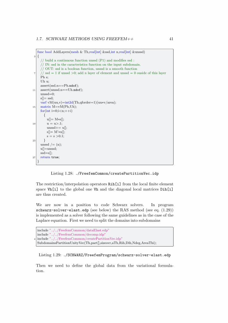
1.7. SCHWARZ METHODS USING FREEFEM++ 41
func bool AddLayers(mesh & Th,real[int] &ssd,int n,real[int] &unssd)3
// build a continuous function uussd (P1) and modifies ssd :// IN: ssd in the caracteristics function on the input subdomain.// OUT: ssd is a boolean function, unssd is a smooth function
7 // ssd = 1 if unssd >0; add n layer of element and unssd = 0 ouside of this layerPh s;Uh u;assert(ssd.n==Ph.ndof);
11 assert(unssd.n==Uh.ndof);unssd=0;s[]= ssd;varf vM(uu,v)=int2d(Th,qforder=1)(uu∗v/area);
15 matrix M=vM(Ph,Uh);for(int i=0;i<n;++i)
u[]= M∗s[];19 u = u>.1;
unssd+= u[];s[]= M’∗u[];s = s >0.1;
23 unssd /= (n);u[]=unssd;ssd=s[];
27 return true;
Listing 1.28: ./FreefemCommon/createPartitionVec.idp
The restriction/interpolation operators Rih[i] from the local finite elementspace Vh[i] to the global one Vh and the diagonal local matrices Dih[i]
are thus created.
We are now in a position to code Schwarz solvers. In programschwarz-solver-elast.edp (see below) the RAS method (see eq. (1.29))is implemented as a solver following the same guidelines as in the case of theLaplace equation. First we need to split the domains into subdomains
include ”../../FreefemCommon/dataElast.edp”include ”../../FreefemCommon/decomp.idp”
4 include ”../../FreefemCommon/createPartitionVec.idp”SubdomainsPartitionUnityVec(Th,part[],sizeovr,aTh,Rih,Dih,Ndeg,AreaThi);
Listing 1.29: ./SCHWARZ/FreefemProgram/schwarz-solver-elast.edp
Then we need to define the global data from the variational formula-tion.
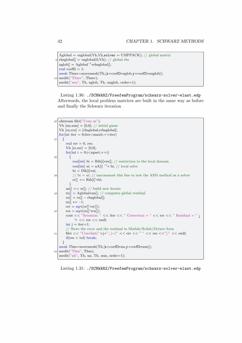
42 CHAPTER 1. SCHWARZ METHODS
Aglobal = vaglobal(Vh,Vh,solver = UMFPACK); // global matrix9 rhsglobal[] = vaglobal(0,Vh); // global rhs
uglob[] = Aglobal−1∗rhsglobal[];real coeff2 = 1;mesh Thmv=movemesh(Th,[x+coeff2∗uglob,y+coeff2∗uuglob]);
13 medit(”Thmv”, Thmv);medit(”uex”, Th, uglob, Th, uuglob, order=1);
Listing 1.30: ./SCHWARZ/FreefemProgram/schwarz-solver-elast.edpAfterwords, the local problem matrices are built in the same way as beforeand finally the Schwarz iteration
27 ofstream filei(”Conv.m”);Vh [un,uun] = [0,0]; // initial guessVh [rn,rrn] = [rhsglobal,rrhsglobal];for(int iter = 0;iter<maxit;++iter)
31 real err = 0, res;Vh [er,eer] = [0,0];for(int i = 0;i<npart;++i)
35 real[int] bi = Rih[i]∗rn[]; // restriction to the local domain
real[int] ui = aA[i] −1∗ bi; // local solvebi = Dih[i]∗ui;
39 // bi = ui; // uncomment this line to test the ASM method as a solverer[] += Rih[i]’∗bi;
un[] += er[]; // build new iterate
43 rn[] = Aglobal∗un[]; // computes global residualrn[] = rn[] − rhsglobal[];rn[] ∗= −1;err = sqrt(er[]’∗er[]);
47 res = sqrt(rn[]’∗rn[]);cout << ”Iteration: ” << iter << ” Correction = ” << err << ” Residual = ” ⤸
Ç << res << endl;int j = iter+1;// Store the error and the residual in Matlab/Scilab/Octave form
51 filei << ”Convhist(”+j+”,:)=[” << err << ” ” << res <<”];” << endl;if(res < tol) break;
mesh Thm=movemesh(Th,[x+coeff2∗un,y+coeff2∗uun]);
55 medit(”Thm”, Thm);medit(”uh”, Th, un, Th, uun, order=1);
Listing 1.31: ./SCHWARZ/FreefemProgram/schwarz-solver-elast.edp

Chapter 2
Optimized Schwarz methods(OSM)
During the last decades, a new class of non-overlapping and overlappingSchwarz methods was developed for partial differential equations, namelythe optimized Schwarz methods. These methods are based on a classicaldomain decomposition, but they use more effective transmission conditionsthan the classical Dirichlet conditions at the interfaces between subdomains.
We first introduce P.L. Lions’ domain decomposition method [129] in § 2.1.Instead of solving a Dirichlet or Neumann boundary value problem (BVP)in the subdomains as in Schwarz or FETI/BNN algorithms, a Robin (a.k.aas mixed) BVP is solved. We compute the convergence factor of the methodand give a general convergence proof. This algorithm was extended toHelmholtz problem by Despres [45], see § 2.2. This extension is all themore important since the original Schwarz method is not convergent in thecase of wave propagation phenomena in the frequency regime. Implementa-tion issues are discussed in § 2.3. In particular, when subdomains overlapOSM can be implemented simply by replacing the Dirichlet solves in ASMwith Robin solves. This justifies the “S” in OSM. Then, in sections 2.4 and2.5, we show that it is possible to consider other interface conditions thanRobin conditions and optimize their choice with respect to the convergencefactor. This explains the “O” in OSM. In the last section 2.6, we explain aFreeFem++ implementation.
2.1 P.L. Lions’ Algorithm
For elliptic problems, Schwarz algorithms work only for overlapping domaindecompositions and their performance in terms of iterations counts dependson the width of the overlap. Substructuring algorithms such as BNN (Bal-ancing Neumann-Neumann [132]) or FETI (Finite Element Tearing and In-
43

44 CHAPTER 2. OPTIMIZED SCHWARZ METHODS (OSM)
1 2n1
n21 2n1n2
Figure 2.1: Outward normals for overlapping and non overlapping subdo-mains for P.L. Lions’ algorithm.
terconnecting [80]) are defined for non overlapping domain decompositionsbut not for overlapping subdomains. The algorithm introduced by P.L. Lions[129] can be applied to both overlapping and non overlapping subdomains.It is based on improving Schwarz methods by replacing the Dirichlet inter-face conditions by Robin interface conditions. Let α be a positive number,the modified algorithm reads
−∆(un+11 ) = f in Ω1,
un+11 = 0 on ∂Ω1 ∩ ∂Ω,
( ∂
∂n1+ α) (un+1
1 ) = ( ∂
∂n1+ α) (un2) on ∂Ω1 ∩Ω2 ,
(2.1)
and
−∆(un+12 ) = f in Ω2,
un+12 = 0 on ∂Ω2 ∩ ∂Ω
( ∂
∂n2+ α) (un+1
2 ) = ( ∂
∂n2+ α) (un1) on ∂Ω2 ∩Ω1
(2.2)
where n1 and n2 are the outward normals on the boundary of the subdo-mains, see Figure 2.1.
We use Fourier transform to analyze the benefit of the Robin interface con-ditions in a simple case. The domain Ω = R2 is decomposed into two half-planes Ω1 = (−∞, δ) × R and Ω2 = (0,∞) × R with δ ≥ 0. We consider theexample of a symmetric positive definite problem
(η −∆)(u) = f in R2,
with η being a positive constant. The algorithm can be written as:
(η −∆)(un+11 ) = f(x, y), (x, y) ∈ Ω1
un+11 is bounded at infinity
( ∂
∂n1+ α) (un+1
1 )(δ, y) = ( ∂
∂n1+ α) (un2)(δ, y), y ∈ R
(2.3)
2.1. P.L. LIONS’ ALGORITHM 45
and
(η −∆)(un+12 ) = f(x, y), (x, y) ∈ Ω2
un+12 is bounded at infinity
( ∂
∂n2+ α) (un+1
2 )(0, y) = ( ∂
∂n2+ α) (un1)(0, y), y ∈ R
(2.4)
2.1.1 Computation of the convergence factor
In order to compute the convergence factor of the algorithm given by (2.3)and (2.4) we introduce the errors eni = uni − u∣Ωi , i = 1,2. By linearity, theerrors satisfy (2.3) and (2.4) with f = 0:
(η −∆)(en+11 ) = 0, (x, y) ∈ Ω1
en+11 is bounded at infinity
( ∂
∂n1+ α) (en+1
1 )(δ, y) = ( ∂
∂n1+ α) (en2)(δ, y), y ∈ R
(2.5)
and
(η −∆)(en+12 ) = 0, (x, y) ∈ Ω2
en+12 is bounded at infinity
( ∂
∂n2+ α) (en+1
2 )(0, y) = ( ∂
∂n2+ α) (en1)(0, y), y ∈ R
(2.6)
By taking the partial Fourier transform of the first line of (2.5) in the ydirection we get:
(η − ∂2
∂x2+ k2)(en+1
1 (x, k)) = 0 for x < δ and k ∈ R.
For a given k, this is an ODE whose solution is sought in the form
∑j γj(k) exp(λj(k)x). A simple calculation shows that lambda is neces-sarily given by:
λ±(k) = ±√η + k2.
Therefore we have
en+11 (x, k) = γn+1
+ (k) exp(λ+(k)x) + γn+1− (k) exp(λ−(k)x).
From the second line of (2.5), the solution must be bounded at x = −∞.This implies that γn+1
− (k) ≡ 0. Thus we have
en+11 (x, k) = γn+1
+ (k) exp(λ+(k)x)
or equivalently, by changing the value of the coefficient γ+,
en+11 (x, k) = γn+1
1 (k) exp(λ+(k)(x − δ))
46 CHAPTER 2. OPTIMIZED SCHWARZ METHODS (OSM)
and similarly for subdomain 2,
en+12 (x, k) = γn+1
2 (k) exp(λ−(k)x)
with γn+11,2 to be determined. From the interface conditions we get
γn+11 (k)(λ+ + α) = γn2 (k)(λ− + α) exp(λ−(k)δ)
and
γn+12 (k)(−λ− + α) = γn1 (k)(−λ+ + α) exp(−λ+(k)δ).
Combining these two and denoting λ(k) = λ+(k) = −λ−(k), we get for i = 1,2,
γn+1i (k) = ρ(k, δ;α)2γn−1
i (k)
with
ρ(k, δ;α) = ∣λ(k) − αλ(k) + α ∣ exp(−λ(k)δ) (2.7)
where λ(k) =√η + k2 and α > 0.
Remark 2.1.1 Formula (2.7) deserves a few remarks.
• With or without overlap, f For all k ∈ R, ρ(k, δ;α) < 1 so that γni (k)→0 as n goes to infinity. The method is convergent.
• When domains overlap (δ > 0), ρ(k, δ;α) is uniformly bounded fromabove by a constant smaller than one, ρ(k, δ;α) < exp(−√η δ) < 1 andρ→ 0 as k tends to infinity. Convergence is geometric.
• When there is no overlap (δ = 0), ρ→ 1 as k tends to infinity.
• Let kc ∈ R. By taking α = λ(kc), we have ρ(kc) = 0.
• For the original Schwarz method (1.3), the convergence factor isexp(−λ(k)δ) and for δ = 0 we see once again that there is no con-vergence. Replacing the Dirichlet interface conditions (ICs) by Robinconditions enhances the convergence of the k-th component of the errorto zero by an improvement factor
ρ(k,0;α) = ∣λ(k) − αλ(k) + α ∣ < 1 . (2.8)

2.1. P.L. LIONS’ ALGORITHM 47
0
0.2
0.4
0.6
0.8
1
0 5 10 15 20 25 30 35 40
Co
nve
rge
nce
Ra
te
Fourier number
with Robin interface conditionsDirichlet interface conditions
0
0.2
0.4
0.6
0.8
1
0 5 10 15 20 25 30 35 40
Fourier number
Improvement factor
Figure 2.2: Left: Convergence factor (dotted line: Dirichlet ICs, solid line:Robin ICs) vs. Fourier number.Right: Improvement factor due to Robin interface conditions (2.8) vs.Fourier number
2.1.2 General convergence proof
The convergence proof given by P.L. Lions in the elliptic case [129] was ex-tended by B. Despres [45] to Helmholtz equation and then to time-harmonicMaxwell equations [47]. A general presentation for these equations is givenin [35]. We treat here the elliptic case with interface conditions (IC)more general than Robin IC since they involve second order tangentialderivatives along the interfaces. Our proof is formal since no functionalanalysis framework is given. Nevertheless, this general convergence resultshows the robustness of this approach in the non overlapping case.
Let Ω be an open set, we consider the following problem:
η(x)u −∇ ⋅ (κ(x)∇u) = f in Ω,u = 0 on ∂Ω,
where the functions x↦ η(x), κ(x) are positive functions.
The domain is decomposed into N non-overlapping subdomains (Ωi)1≤i≤N ,
Ω = ∪Ni=1Ωi and Ωi ∩Ωj = ∅, for i ≠ j.Let Γij denote the interface Γij = ∂Ωi ∩ ∂Ωj , i ≠ j. For two disjointssubdomains, we have Γij = ∅.
For sake of simplicity in the writing of the interface conditions, we considerthe two dimensional case (Ω ⊂ R2) although the proof is valid in arbitrarydimension. The interface conditions include second order tangential deriva-tives and have the form
Bij ∶= κ(x)∂
∂ni+Λij , Λij ∶= αij(x) − ∂
∂τi(βij(x)
∂
∂τi) (2.9)

48 CHAPTER 2. OPTIMIZED SCHWARZ METHODS (OSM)
where αij and βij are functions from Γij into R that verify
αij(x) = αji(x) ≥ α0 > 0,
βij(x) = βji(x) ≥ 0
βij(x) = 0 on ∂Γij .
In this case the operators Λij = Λji defined in (2.9) have the following re-markable properties
• Λij is SPD (symmetric positive definite).
• Λij has an invertible SPD square root, denoted by Λ1/2ij whose inverse
is denoted by Λ−1/2ij , which is SPD as well.
The algorithm consists in computing the iterates un+1i of the local solutions
from the previous iterates uni by solving
η(x)un+1i −∇ × (κ(x)∇un+1
i ) = f in Ωi,
un+1i = 0 on ∂Ω ∩ ∂Ωi
(κ(x) ∂
∂ni+Λij)un+1
i = (−κ(x) ∂
∂nj+Λij)unj on Γij .
(2.10)The interface condition in the algorithm (2.10) can be rewritten as
Λ−1/2ij (κ(x)∂ui
∂ni) +Λ
1/2ij (ui) = −Λ
−1/2ij (κ(x)∂uj
∂nj) +Λ
1/2ij (uj) on Γij .
(2.11)The convergence proof of the algorithm (2.10) follows the arguments givenin [35] and is based on a preliminary result which is an energy estimate
Lemma 2.1.1 (Energy Estimate) Let u denote a function that satisfies
η(x)u −∇ ⋅ (κ(x)∇u) = 0 in Ωi
u = 0 on ∂Ωi ∩ ∂Ω,
Then,
∫Ωiη(x)∣ui∣2 + κ(x)∣∇ui∣2 +
1
4∑j≠i∫
Γij(Λ
−1/2ij [κ(x)∂ui
∂ni−Λij(ui)])
2
= 1
4∑j≠i∫
Γij(Λ
−1/2ij [κ(x)∂ui
∂ni+Λij(ui)])
2
Proof From the variational formulation of the local problem
η(x)ui −∇ ⋅ (κ(x)∇ui) = 0 in Ωi,
2.1. P.L. LIONS’ ALGORITHM 49
we get by choosing the test function equal to ui and integrating by parts:
∫Ωiη(x)∣ui∣2 + κ(x)∣∇ui∣2 = ∫
∂Ωiκ(x)∂ui
∂niui =∑
j≠i∫
Γijκ(x)∂ui
∂niui
= ∑j≠i∫
Γijκ(x)∂ui
∂niΛ−1/2ij Λ
1/2ij (ui)
= ∑j≠i∫
ΓijΛ−1/2ij (κ(x)∂ui
∂ni) Λ
1/2ij (ui)
From the identity ab = 14((a + b)2 − (a − b)2), we infer
∫Ωiη(x)∣ui∣2 + κ(x)∣∇ui∣2 +∑
j≠i
1
4∫
Γij(Λ
−1/2ij (κ(x)∂ui
∂ni) −Λ
1/2ij (ui))
2
=∑j≠i
1
4∫
Γij(Λ
−1/2ij (κ(x)∂ui
∂ni) +Λ
1/2ij (ui))
2
which leads to the conclusion.We are ready to prove the following convergence result
Theorem 2.1.1 The algorithm (2.10) converges in H1, that is
limn→∞
∥uni − u∣Ωi∥H1(Ωi) = 0 for i = 1, . . . ,N
Proof In order to prove the convergence of the algorithm we prove thateni = uni − uΩi converges to zero. By linearity of the equations and of thealgorithm, it is clear that the error en+1
i satisfies
η(x)en+1i −∇ ⋅ (κ(x)∇en+1
i ) = 0 in Ωi,en+1i = 0 on ∂Ω ∩ ∂Ωi
Λ−1/2ij (κ(x)∂e
n+1i
∂ni) +Λ
1/2ij (en+1
i ) = −Λ−1/2ij (κ(x) ∂e
nj
∂nj) +Λ
1/2ij (enj ) on Γij .
We apply the energy estimate to en+1i and taking into account the interface
condition (2.11) and noticing that by assumption we have Λij = Λji, we get
∫Ωiη(x)∣en+1
i ∣2 + κ(x)∣∇en+1i ∣2 = ∑
j≠i
1
4∫
Γij(Λ
−1/2ji (−κ(x)
∂enj
∂nj) +Λ
1/2ji (enj ))
2
− (Λ−1/2ij (κ(x)∂e
n+1i
∂ni) −Λ
1/2ij (en+1
i ))2
(2.12)We introduce the following notations:
En+1i ∶= ∫
Ωiη(x)∣en+1
i ∣2 + κ(x)∣∇en+1i ∣2,
Cn+1ij ∶= 1
4∫
Γij(Λ
−1/2ij (κ(x)∂e
n+1i
∂ni) −Λ
1/2ij (en+1
i ))2
En+1 =N
∑i=1
En+1i , Cn = ∑
i,j(j≠i)
Cnji.

50 CHAPTER 2. OPTIMIZED SCHWARZ METHODS (OSM)
With these notations, estimate (2.12) can be re-written as
En+1i +∑
j≠i
Cn+1ij =∑
j≠i
Cnji.
After summation over the subdomains, we have
N
∑i=1
En+1i + ∑
i,j(j≠i)
Cn+1ij = ∑
i,j(j≠i)
Cnji = ∑i,j(j≠i)
Cnij .
Let us denote
En+1 ∶=N
∑i=1
En+1i and Cn ∶= ∑
i,j(j≠i)
Cnji ,
we haveEn+1 + Cn+1 = Cn.
Hence, by summation over n, we get
∞
∑n=0
En+1 ≤ C0.
This series is convergent only if En → 0 as n →∞, which proves that for allsubdomain 1 ≤ i ≤ N we have necessarily eni → 0 in H1 norm as n tends toinfinity.
The same kind of proof holds for the Maxwell system [47] and the convection-diffusion equation [145].
2.2 Helmholtz problems
We have considered so far domain decomposition methods for Poisson orelasticity problems which yield symmetric positive definite matrices. With asuitable coarse space, Schwarz or BNN/FETI type methods are very power-ful methods whose scalability can be proven. But, the numerical simulationof propagation phenomena via Helmholtz equations, Maxwell and elasticitysystems in the frequency domain yield matrices which are symmetric butnot positive. The extension of P.L. Lions algorithm to Helmholtz problemin [45], § 2.2.2, is the first iterative method with proven convergence for thisindefinite operator.
2.2.1 Convergence issues of the Schwarz method forHelmholtz
The Helmholtz equation is derived from the acoustic wave equation:
1
c2
∂2u
∂t2−∆u = f(t, x, y)

2.2. HELMHOLTZ PROBLEMS 51
which models for instance pressure variation with a source term f and asound velocity c. When the source is time periodic, it makes sense to lookfor time periodic solutions as well. With some abuse of notation, let f =f(x, y) exp(iωt) (i2 = −1) be a harmonic source term of frequency ω, we seekthe solution to the acoustic wave equation in the form u = u(x, y) exp(iωt).Then, u must be a solution to the Helmholtz equation
L(u) ∶= (−ω2
c2−∆)(u) = f(x, y), x, y ∈ Ω
whose solution is in general complex valued.
An extra difficulty comes from the non positivity of the Helmholtz operatordue to the negative sign of the term of order zero. More precisely, a Schwarzalgorithm for solving Helmholtz equation involves the decomposition of do-main Ω into N overlapping subdomains (Ωj)1≤j≤N , the solving of Dirichletproblems in the subdomains:
(−ω2
c2−∆)(un+1
j ) = f(x, y), in Ωj , 1 ≤ j ≤ Nun+1j = un, on ∂Ωj
(2.13)
and then using a partition of unity (ξj)1≤j≤N related to (Ωj)1≤j≤N :
un+1 ∶=N
∑j=1
ξj un+1j .
The problem is that this algorithm is not necessarily well-posed. Indeed,if ω2/c2 is an eigenvalue of the Poisson operator in a subdomain Ωk, thereexists a non zero function vk ∶ Ωk → R such that:
−∆vk = ω2
c2vk in Ωk
vk = 0 on ∂Ωk .
Then, problem (2.13) is ill-posed in subdomain Ωk. Either there is nosolution to it or if there is one, it is possible to add to it any functionproportional to the eigenvalue vk and still satisfy equation (2.13). We havehere what is called a Fredholm alternative.
Moreover, even when the local problems are well-posed, a bad convergence isto be expected. We present the analysis in the case of the plane divided intotwo subdomains although it is very similar to the elliptic case considered in§ 1.5.2. We introduce the wave number
ω ∶= ωc.
52 CHAPTER 2. OPTIMIZED SCHWARZ METHODS (OSM)
Consider the domain is Ω = R2 with the Sommerfeld radiation condition atinfinity,
limr→∞
√r (∂u
∂r+ iωu) = 0,
where r =√x2 + y2. We decompose it into two subdomains with or without
overlap, δ ≥ 0, Ω1 = (−∞, δ ) × R and Ω2 = (0,∞) × R and consider theSchwarz algorithm
−∆un+11 − ω2un+1
1 = f(x, y), x, y ∈ Ω1
un+11 (δ, y) = un2(δ, y) , ∀y ∈ R
limr→∞
√r (∂u
n+11
∂r+ iωun+1
1 ) = 0
(2.14)
and−∆un+1
2 − ω2un+12 = f(x, y), x, y ∈ Ω2
un+12 (0, y) = un1(0, y) , ∀y ∈ R
limr→∞
√r (∂u
n+12
∂r+ iωun+1
2 ) = 0 .
(2.15)
For the convergence analysis it suffices by linearity to consider the casef(x, y) = 0 and to analyze convergence to the zero solution. Let the Fouriertransform in y direction be denoted by
u(x, k) ∶= (Fu)(x, k) = ∫Ru(x, y)e−ikydy,
Taking a Fourier transform of the algorithms (2.14) and (2.15) in the ydirection we obtain
−∂2un+1
1
∂x2− (ω2 − k2)un+1
1 = 0,
x < δ, k ∈ R (2.16)un+1
1 (δ, k) = un2(δ, k)
and
−∂2un+1
2
∂x2− (ω2 − k2)un+1
2 = 0,
x > 0, k ∈ R (2.17)un+1
2 (0, k) = un1(0, k)
The general solutions of these ordinary differential equations are
un+1j = Ajeλ(k)x +Bje−λ(k)x, j = 1,2,
where λ(k) denotes the root of the characteristic equation λ2 + (ω2 −k2) = 0with positive real or imaginary part,
λ(k) = √k2 − ω2 for ∣k∣ ≥ ω,
i√ω2 − k2 for ∣k∣ < ω.
(2.18)

2.2. HELMHOLTZ PROBLEMS 53
Note that the main difference with the elliptic case is that λ(k) is a complexvalued function. It takes real values for the vanishing modes ∣k∣ ≥ ω andpurely imaginary values for propagative modes ∣k∣ < ω. Since the Sommerfeldradiation condition excludes growing solutions as well as incoming modes atinfinity, we obtain the local solutions
un+11 (x, k) = un+1
1 (δ, k)eλ(k)(x−δ)un+1
2 (x, k) = un+12 (0, k)e−λ(k)x. (2.19)
Then, it is easy to check that
un+11 (δ, k) = exp (−2λ(k) δ) un−1
1 (δ, k).
Defining the convergence factor ρ by
ρ(k, δ) ∶= ∣ un+11 (δ, k)un−1
1 (δ, k)∣1/2
(2.20)
we find by plugging (2.19) into (2.14) and (2.15) that
ρ(k, δ) = ∣ exp (−λ(k) δ)∣ (2.21)
where λ(k) is given by (2.18). By induction, the following result follows foreven n
∣un1(0, k)∣ = ∣ρ(k, δ)nu01(0, k), un2(0, k)∣ = ∣ρ(k, δ)nu0
2(0, k)∣ .
Remark 2.2.1 We can distinguish a few features from the expression of theconvergence factor, see Figure 2.3:
• The main difference with the elliptic case is that ρ(k, δ) is a complexvalued function. The convergence will occur if the modulus of ρ issmaller than one, ∣ρ(k, δ)∣ < 1.
• For vanishing modes ∣k∣ > ω, λ(k) is negative and real so that thesemodes converge faster for larger overlaps. But we have ∣ρ(k, δ)∣ ≡ 1 forpropagative modes ∣k∣ < ω whatever the overlap is since there λ(k) ∈iR. This prevents the convergence of the Schwarz algorithm for theHelmholtz equation.
• A possible fix is the use of a relaxation parameter θ:
un+1i ∶= θun+1
i + (1 − θ)uni .
The choice of the optimal parameter θ is not easy and the overallconvergence rate is not good anyway.
It is thus clear that the Schwarz method cannot be used safely nor efficientlyas a solver for the Helmholtz equation.

54 CHAPTER 2. OPTIMIZED SCHWARZ METHODS (OSM)
0
0.2
0.4
0.6
0.8
1
1.2
0 5 10 15 20 25 30 35 40
Fourier number
Convergence rate for omega = 10
Figure 2.3: Convergence factor (2.21) of the Schwarz method for Helmholtzequation vs. Fourier number
2.2.2 Despres’ Algorithm for the Helmholtz equation
The algorithm by P.L. Lions can be applied to the Helmholtz equation withthe choice α = iω (i2 = −1). We give here a slight modification of theoriginal algorithm given in [44]. Domain Ω is decomposed intoN overlappingsubdomains (Ωj)1≤j≤N and at each iteration a subdomain solve reads
(−ω2 −∆)(un+1j ) = f(x, y) in Ωj , 1 ≤ j ≤ N
( ∂
∂nj+ iω)(un+1
j ) = ( ∂
∂nj+ iω)(un) on ∂Ωj
(2.22)
and then using a partition of unity (ξj)1≤j≤N related to (Ωj)1≤j≤N :
un+1 ∶=N
∑j=1
ξj un+1j .
This algorithm fixes the two drawbacks of the Schwarz algorithm explainedin § 2.2.1. First, note that the solution to the boundary value problem (2.22)is unique even if ω2 is an eigenvalue of the Laplace operator with Dirichletboundary conditions. Indeed, suppose for some subdomain Ωk (1 ≤ k ≤ N)we have a function v ∶ Ωk → C that satisfies:
−ω2v −∆v = 0 in Ωk
( ∂
∂nk+ iω) (v) = 0 on ∂Ωk .

2.2. HELMHOLTZ PROBLEMS 55
Multiplying the equation by the conjugate of v and integrating by parts, weget:
∫Ωk−ω2∣v∣2 + ∣∇v∣2 − ∫
∂Ωk
∂v
∂nkv = 0 .
Taking into account the Robin condition on ∂Ωk, we have:
∫Ωk−ω2∣v∣2 + ∣∇v∣2 + ∫
∂Ωki ω∣v∣2 = 0 .
Taking the imaginary part of the above equality, we get:
∫∂Ωk
ω∣v∣2 = 0 ,
so that v is zero on ∂Ωk. Using again the Robin condition, we have that∂v/∂nk = 0 as well on ∂Ωk. Together with the fact that −ω2v − ∆v = 0 inΩk, a unique continuation principle proves that v is identically zero in Ω.Thus Despres algorithm is always well defined.The second point is that convergence of algorithm was proved in [46] for anon overlapping decomposition of domain Ω. It is worth noticing that it wasthe first time an iterative solver with proven convergence was proposed forthe Helmholtz and subsequently Maxwell equations [47]. For overlappingsubdomains, no general convergence proof is available. But, in the case ofthe plane R2 decomposed into two overlapping half-planes, the convergencefactor can be computed and a convergence result follows. The algorithmstudied here can be written as
−∆un+11 − ω2un+1
1 = f(x, y), x, y ∈ Ω1
( ∂
∂n1+ iω) (un+1
1 )(δ, y) = ( ∂
∂n1+ iω)un2(δ, y) , ∀y ∈ R
limr→∞
√r (∂u
n+11
∂r+ iωun+1
1 ) = 0
(2.23)
and
−∆un+12 − ω2un+1
2 = f(x, y), x, y ∈ Ω2
( ∂
∂n2+ iω)un+1
2 (0, y) = ( ∂
∂n2+ iω)un1(0, y) , ∀y ∈ R
limr→∞
√r (∂u
n+12
∂r+ iωun+1
2 ) = 0 .
(2.24)
Performing a convergence analysis as in § 2.1, the convergence factor is:
ρ(k, δ) = ∣λ(k) − iωλ(k) + iω ∣ ∣ exp(−λ(k) δ)∣ (2.25)

56 CHAPTER 2. OPTIMIZED SCHWARZ METHODS (OSM)
0
0.2
0.4
0.6
0.8
1
1.2
0 5 10 15 20 25 30 35 40
Fourier number
Convergence rate for omega = 10
Figure 2.4: Convergence factor (2.25) of Despres method for Helmholtzequation vs. Fourier number (δ = 0.1)
where λ(k) is given by formula (2.18). Note that we have
ρ(k, δ) =
⎧⎪⎪⎪⎪⎪⎪⎨⎪⎪⎪⎪⎪⎪⎩
∣√ω2 − k2 − ω√ω2 − k2 + ω
∣ , for ∣k∣ < ∣ω∣,
exp(−√k2 − ω2δ), for ∣k∣ < ∣ω∣ ,
see Figure 2.4. Note that for propagative modes ∣k∣ < ∣ω∣, ∣ exp(−λ(k)δ)∣ =1 since λ(k) is purely imaginary. Therefore the convergence comes fromthe Robin condition independently of the overlap. As for vanishing modes∣k∣ > ∣ω∣, λ is real. The modulus of the rational fraction in (2.25) is 1 andconvergence comes from the overlap. Thus for all Fourier modes except ∣k∣ =ω, the convergence factor is smaller than one. Thus, the method convergesfor almost every Fourier number k.
2.3 Implementation issues
A Robin boundary value problem is different from standard Dirichlet orNeumann problems but poses no difficulty as long as the right-hand side ofthe Robin condition is known. But as we shall see, the discretization of theright-hand side (2.26) on an interface is not a trivial task. Fortunately, itmay be eased by tricks explained in § 2.3.1 and 2.3.2.
2.3. IMPLEMENTATION ISSUES 57
Consider for example the problem (2.1) in Lions’ algorithm and let gn2 denotethe right-hand side on the interface of subdomain Ω1:
gn2 ∶= ( ∂
∂n1+ α) (un2) on ∂Ω1 ∩ Ω2 . (2.26)
Then, the bilinear form associated to the variational formulation of (2.1) is:
aRobin ∶ H1(Ω1) ×H1(Ω1) Ð→ R(u, v) z→ ∫
Ω1
(ηuv +∇u ⋅ ∇v) + ∫∂Ω1∩Ω2
αuv .
(2.27)Note that the boundary integral term containing α is positive when v = u.Thus bilinear form aRobin is even more coercive than the one associated withthe Neumann boundary value problem which contains only the subdomainintegral term. The linear form related to (2.1) reads:
lRobin ∶ H1(Ω1) Ð→ Rv z→ ∫
Ω1
f v + ∫∂Ω1∩Ω2
gn2 v .(2.28)
The variational formulation of the Robin boundary value problem reads:
Find u ∈H1(Ω1) such that∀v ∈H1(Ω1), aRobin(u, v) = lRobin(v) .
The finite element discretization is simply obtained by replacing the infinitedimensional Sobolev space H1(Ω1) by a finite dimensional space for examplea classical P1 finite element space denoted Vh(Ω1):
Find u ∈ Vh(Ω1) such that∀vh ∈ Vh(Ω1), aRobin(uh, vh) = lRobin(vh) .
From an algebraic point of view, we consider a finite element basis
φk∣k ∈ N1 ⊂ Vh(Ω1)
where N1 is the set of degrees of freedom. The matrix form of aRobin,h isdenoted by ARobin,1:
[ARobin,1]kl ∶= aRobin,h(φl, φk) = ∫Ω1
(ηφlφk +∇φl ⋅ ∇φk) + ∫∂Ω1∩Ω2
αφl φk .
(2.29)Matrix ARobin,1 is actually the sum of the mass matrix, a stiffness matrixwhich corresponds to a Neumann problem and of a matrix that has zero
entries for interior degrees of freedom (
Supp φk ∩ (∂Ω1 ∩Ω2) = ∅), see equa-tion (2.39) as well.Note that the same technique can be applied in the case of the Despres’algorithm for the Helmholtz equation with minimal adjustements due to
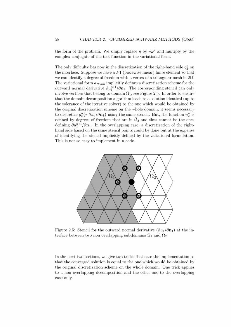
58 CHAPTER 2. OPTIMIZED SCHWARZ METHODS (OSM)
the form of the problem. We simply replace η by −ω2 and multiply by thecomplex conjugate of the test function in the variational form.
The only difficulty lies now in the discretization of the right-hand side gn2 onthe interface. Suppose we have a P1 (piecewise linear) finite element so thatwe can identify a degree of freedom with a vertex of a triangular mesh in 2D.The variational form aRobin implicitly defines a discretization scheme for theoutward normal derivative ∂un+1
1 /∂n1. The corresponding stencil can onlyinvolve vertices that belong to domain Ω1, see Figure 2.5. In order to ensurethat the domain decomposition algorithm leads to a solution identical (up tothe tolerance of the iterative solver) to the one which would be obtained bythe original discretization scheme on the whole domain, it seems necessaryto discretize gn2 (= ∂un2 /∂n1) using the same stencil. But, the function un2 isdefined by degrees of freedom that are in Ω2 and thus cannot be the onesdefining ∂un+1
1 /∂n1. In the overlapping case, a discretization of the right-hand side based on the same stencil points could be done but at the expenseof identifying the stencil implicitly defined by the variational formulation.This is not so easy to implement in a code.
1 2
Figure 2.5: Stencil for the outward normal derivative (∂u1/∂n1) at the in-terface between two non overlapping subdomains Ω1 and Ω2
In the next two sections, we give two tricks that ease the implementation sothat the converged solution is equal to the one which would be obtained bythe original discretization scheme on the whole domain. One trick appliesto a non overlapping decomposition and the other one to the overlappingcase only.

2.3. IMPLEMENTATION ISSUES 59
2.3.1 Two-domain non-overlapping decomposition
This section is concerned with the Finite Element implementation of theinterface conditions of Robin type for a non-overlapping decomposition ofthe domain. We present the discretization scheme for a decomposition of adomain Ω into two non overlapping subdomains Ω1 and Ω2 with interfaceΓ12. We consider first the optimized Schwarz algorithm at the continuouslevel,
(η −∆)un+11 = f in Ω1
∂un+11
∂n1+ αun+1
1 = −∂un2
∂n2+ αun2 on Γ12
(2.30)(η −∆)un+1
2 = f in Ω2
∂un+12
∂n2+ αun+1
2 = −∂un1
∂n1+ αun1 on Γ12.
where we have used that on the interface between non overlapping subdo-mains, we have n1 = −n2, see Figure 2.1. A direct discretization wouldrequire the computation of the normal derivatives along the interfaces in or-der to evaluate the right-hand sides in the transmission conditions of (2.30).This can be avoided by re-naming the problematic quantities:
λn1 = −∂un2
∂n2+ αun2 and λn2 = −∂u
n1
∂n1+ αun1 .
The algorithm (2.30) becomes
(η −∆)un+11 = f in Ω1
∂un+11
∂n1+ αun+1
1 = λn1 on Γ12
(2.31)(η −∆)un+1
2 = f in Ω2
∂un+12
∂n2+ αun+1
2 = λn2 on Γ12
λn+11 =−λn2 + 2αun+1
2
λn+12 =−λn1 + 2αun+1
1 .
The last two update relations of (2.31) follow from:
λn+11 ∶= −∂u
n+12
∂n2+ αun+1
2 = −(∂un+12
∂n2+ αun+1
2 ) + 2αun+12 = −λn2 + 2αun+1
2
(2.32)and similarly
λn+12 ∶= −∂u
n+11
∂n1+ αun+1
1 = −(∂un+11
∂n1+ αun+1
1 ) + 2αun+11 = −λn1 + 2αun+1
1 .
(2.33)
60 CHAPTER 2. OPTIMIZED SCHWARZ METHODS (OSM)
Equations (2.32) and (2.33) can be interpreted as a fixed point algorithm inthe new variables λj , j = 1,2, to solve the substructured problem
λ1 = −λ2 + 2αu2(λ2, f) ,λ2 = −λ1 + 2αu1(λ1, f) ,
(2.34)
where uj = uj(λj , f), j = 1,2, are solutions of:
(η −∆)uj = f in Ωj ,
∂uj
∂nj+ αuj = λj on Γ12.
Instead of solving the substructured problem (2.34) by the fixed point itera-tion (2.31), one usually uses a Krylov subspace method to solve the substruc-tured problem. This corresponds to using the optimized Schwarz method asa preconditioner for the Krylov subspace method.At this point, we can introduce the algebraic counterparts of the continu-ous quantities. A finite element discretization of the substructured prob-lem (2.34) leads to the linear system
λ1 = −λ2 + 2αB2u2
λ2 = −λ1 + 2αB1u1(2.35)
where uj = uj(λj ,fj), j = 1,2 are solutions of:
ARobin,1u1 = f1 +BT1 λ1
ARobin,2u2 = f2 +BT2 λ2
(2.36)
We detail now the new matrices and vectors we have introduced:
• Vectors u1, u2 contain the degrees of freedom of the subdomain solu-tions.
• Vectors f1, f2 are the degrees of freedom related to f .
• Matrices B1 and B2 are the trace operators of the domains Ω1 and Ω2
on the interface Γ12.
In order to define matrices ARobin,j , we first split the two vectors u1 and u2
into interior and boundary degrees of freedom:
uj =⎡⎢⎢⎢⎢⎣
uij
ubj
⎤⎥⎥⎥⎥⎦, j = 1,2, (2.37)
where the indices i and b correspond to interior and interface degrees offreedom respectively for domain Ωj . Then the discrete trace operators B1

2.3. IMPLEMENTATION ISSUES 61
and B2 are just the Boolean matrices corresponding to the decomposition(2.37) and they can be written as
Bj = [0 I] , j = 1,2, (2.38)
where I denotes the identity matrix of appropriate size. For example,
B1u1 = ub1 and B2u2 = ub2.
Matrices ARobin,1 and ARobin,2 arise from the discretization of the local η−∆operators along with the interface conditions ∂n + α,
ARobin,j =Kj +BTj αMΓ12Bj , j = 1,2. (2.39)
Here Kj are local matrices of problem (as combination of stiffness and massmatrices) and MΓ12 is the interface mass matrix
[MΓ12]nm = ∫Γ12
φnφm dξ (2.40)
The functions φn and φm are the basis functions associated with the degreesof freedom n and m on the interface Γ12.For given λ1 and λ2, the functions u1 and u2 can be computed by solvingequations (2.36). By eliminating u1 and u2 in (2.35) using (2.36), we obtainthe substructured linear system
Fλ = d, (2.41)
where λ = (λ1,λ2) and the matrix F and the right-hand side d are
F = ( I I − 2αB2A−1Robin,2B
T2
I − 2αB1A−1Robin,1B
T1 I
)
d = (2αB1A−1Robin,1f1
2αB2A−1Robin,2f2.
)(2.42)
The linear system (2.41) is solved by a Krylov subspace method , see Chap-ter 3. The matrix vector product amounts to solving a subproblem in eachsubdomain and to send interface data between subdomains.The general case of a decomposition into an arbitrary number of subdomainsis treated in [91] for the case of the Helmholtz equations. It is also possible todiscretize the interface conditions by using Lagrange multipliers the methodis then named FETI 2 LM (Two-Lagrange Multiplier ), see [167].
2.3.2 Overlapping domain decomposition
The trick explained in the non overlapping case cannot be used in theoverlapping case, see Figure 2.1. Indeed, even in the simple case of two
62 CHAPTER 2. OPTIMIZED SCHWARZ METHODS (OSM)
subdomains, the normal derivatives are computed on two distinct interfaces∂Ω1 ∩ Ω2 and ∂Ω2 ∩ Ω1. Here as well, it is possible to write an algorithmequivalent to P.L. Lions’ algorithm (2.1)-(2.2) but where the iterate is afunction un ∶ Ω→ R i.e. it is not a pair of functions (un1 , un2).
Let a overlapping domain decomposition Ω = Ω1 ∪ Ω2 with a partition ofunity functions χ1 and χ2:
χ1 + χ2 = 1, suppχi ⊂ Ωi, i = 1,2.
Let un ∶ Ω→ R be an approximate solution to a Poisson equation. Then theupdate un+1 is computed by the following algorithm which is the continuousversion of the Optimized Restricted Additive Schwarz (ORAS) algorithm,see [38]. The solution will come from section 1.3 where an equivalence
Algorithm 3 ORAS algorithm at the continuous level
1. Compute the residual rn ∶ Ω→ R:
rn ∶= f − (η −∆)un (2.43)
2. For i = 1,2 solve for a local correction vni :
(η −∆)vni = rn in Ωi
vni = 0 on ∂Ωi ∩ ∂Ω
( ∂
∂ni+ α) (vni ) = 0 on ∂Ωi ∩ Ω3−i
(2.44)
3. Compute an average of the local corrections and update un:
un+1 = un +E1(χ1vn1 ) +E2(χ2v
n2 ) . (2.45)
where (χi)i=1,2 and (Ei)i=1,2 define a partition of unity as in definedin section 1.1 equation (1.4).
between the original Schwarz algorithm and the RAS method was shown atthe continuous level.
Lemma 2.3.1 (Equivalence between Lions’ algorithm and ORAS)The algorithm defined by (2.43), (2.44) and (2.45) is equivalent to theLions’ Schwarz algorithm
Proof The approach is very similar to what is done in Lemma 1.1.2where we prove the equivalence between the Schwarz algorithm and theRAS method. Here, we have to prove the equality
un = E1(χ1un1) +E2(χ2u
n2) ,

2.3. IMPLEMENTATION ISSUES 63
where un1,2 are given by (2.1)-(2.2) and un is given by (2.43)-(2.44)-(2.45).We assume that the property holds for the initial guesses:
u0 = E1(χ1u01) +E2(χ2u
02)
and proceed by induction assuming the property holds at step n of thealgorithm, i.e. un = E1(χ1u
n1) +E2(χ2u
n2). From (2.45) we have
un+1 = E1(χ1(un + vn1 )) +E2(χ2(un + vn2 )) . (2.46)
We prove now that un∣Ω1
+ vn1 = un+11 by proving that un
∣Ω1+ vn1 satisfies (2.1)
as un+11 does. We first note that, using (2.44)-(2.43) we have:
(η −∆)(un + vn1 ) = (η −∆)un + rn = (η −∆)un + f − (η −∆un) = f in Ω1,
( ∂
∂n1+ α) (un + vn1 ) = ( ∂
∂n1+ α) (un) on ∂Ω1 ∩Ω2,
(2.47)It remains to prove that
( ∂
∂n1+ α) (un) = ( ∂
∂n1+ α) (un2) on ∂Ω1 ∩Ω2 .
By the induction hypothesis we have un = E1(χ1un1) + E2(χ2u
n2). On a
neighborhood of ∂Ω1 ∩Ω2 (zone (c) in Figure 2.6), we have χ1 ≡ 0 and thusχ2 ≡ 1. In this neighborhood, their derivatives are zero as well, so that on∂Ω1 ∩Ω2 we have :
( ∂
∂n1+ α) (un) = ( ∂
∂n1+ α) (χ1u
n1 + χ2u
n2) = ( ∂
∂n1+ α) (un2) . (2.48)
Finally from (2.47) and (2.48) we can conclude that un∣Ω1
+vn1 = un+11 satisfies
problem (2.1) and is thus equal to un+11 . The same holds for domain Ω2,
un∣Ω2
+ vn2 = un+12 . Then equation (2.46) reads
un+1 = E1(χ1un+11 ) +E2(χ2u
n+12 )
which ends the proof of the equivalence between P.L. Lions’ algorithm thecontinuous version of the ORAS algorithm.
The advantage of the ORAS method over a direct implementation ofP.L. Lions algorithm is that the Robin boundary condition (2.44) hasa zero right-hand side that needs no discretization. The only drawbackat the discretized level is that the actual overlap is reduced by a meshsize compared to a full discretization of the original P.L. Lions algorithm,see [38] for more details.

64 CHAPTER 2. OPTIMIZED SCHWARZ METHODS (OSM)
1 2n1n2
(a) (b) (c)(a) (c)
Figure 2.6: Function of partition of unity χ1. In zone (a): χ1 ≡ 1, in zone(b): 0 < χ1 < 1 and in zone (c): χ1 ≡ 0.
We now give the algebraic definition of the ORAS method by giving thediscrete counterparts of steps (2.43)-(2.44)-(2.45), see [38]. Let Un ∈ R#N
be an approximate solution to a linear system:
AU = F . (2.49)
The set of degrees of freedom N is decomposed into two subsets N1 and N2.For i = 1,2, let Ri denote the Boolean restriction matrix to Ni and Di definean algebraic partition of unity ∑2
i=1RTi DiRi = Id, as in (1.25).
The update Un+1 is computed in several steps by the following algorithm
1. Compute the residual rn ∈ R#N :
rn ∶= F −AUn (2.50)
2. For i = 1,2 solve for a local correction Vin:
Ai,RobinVni = Ri rn (2.51)
where Ai,Robin is the discretization matrix of a Robin problem as ex-plained in (2.29) or in (2.39).
3. Compute an average of the local corrections and update Un accord-ingly:
Un+1 = Un +RT1 D1 Vn1 +RT2 D2 Vn
2 . (2.52)
The above three steps algorithm can be written more compactly as:
Definition 2.3.1 (ORAS algorithm) The iterative Optimized Restricted

2.4. OPTIMAL INTERFACE CONDITIONS 65
Additive Schwarz (ORAS) algorithm is the preconditioned fixed point itera-tion defined by
Un+1 = Un +M−1ORASrn, rn ∶= F −AUn
where the matrix
M−1ORAS ∶=
2
∑i=1
RTi DiA−1i,RobinRi (2.53)
is called the ORAS preconditioner.
In short, the only difference with the RAS method (1.29) consists in replacingthe local Dirichlet matrices RiAR
Ti by matrices ARobin,i which correspond
to local Robin subproblems.As explained in chapter 3, it is more profitable to use a Krylov methodin place of the above iterative fixed-point algorithm. It consists in solving(2.49) by a Krylov method such as GMRES or BiCGSTAB preconditionedby operator M−1
ORAS .
2.4 Optimal interface conditions
2.4.1 Optimal interface conditions and ABC
Robin boundary conditions are not the most general interface conditions.Rather than give the general conditions in an a priori form, we shall derivethem in this section so as to have the fastest convergence. We establishthe existence of interface conditions which are optimal in terms of iterationcounts. The corresponding interface conditions are pseudo-differential andare not practical. Nevertheless, this result is a guide for the choice ofpartial differential interface conditions. Moreover, this result establishesa link between the optimal interface conditions and artificial boundaryconditions. This is also a help when dealing with the design of interfaceconditions since it gives the possibility to use the numerous papers andbooks published on the subject of artificial boundary conditions, see e.g.[75, 99] or more generally on truncation of infinite domains via the PMLtechnique [119, 29].
We consider a general linear second order elliptic partial differential operatorL and the problem:
L(u) = f, Ωu = 0, ∂Ω.
The domain Ω is decomposed into two subdomains Ω1 and Ω2. We supposethat the problem is regular so that ui ∶= u∣Ωi , i = 1,2, is continuous and hascontinuous normal derivatives across the interface Γi = ∂Ωi ∩ Ωj , i ≠ j. A

66 CHAPTER 2. OPTIMIZED SCHWARZ METHODS (OSM)
Ω1
Ω2
Ω1cΩ2
c
Γ1
Γ2
Figure 2.7: Subdomains and their complements
modified Schwarz type method is considered.
L(un+11 ) = f in Ω1
un+11 = 0 on ∂Ω1 ∩ ∂Ω
µ1∇un+11 .n1 + B1(un+1
1 )= −µ1∇un2 .n2 + B1(un2) on Γ1
L(un+12 ) = f in Ω2
un+12 = 0 on ∂Ω2 ∩ ∂Ω
µ2∇un+12 .n2 + B2(un+1
2 )= −µ2∇un1 .n1 + B2(un1) on Γ2
(2.54)where µ1 and µ2 are real-valued functions and B1 and B2 are operatorsacting along the interfaces Γ1 and Γ2. For instance, µ1 = µ2 = 0 and B1 =B2 = Id correspond to the original Schwarz algorithm (1.3); µ1 = µ2 = 1 andBi = α ∈ R, i = 1,2, has been proposed in [129] by P. L. Lions.The question to which we would like to answer is:
Are there other possibilities in order to have convergence in aminimal number of steps?
In order to answer this question, we note that by linearity, the error e satisfies(we supposed here with no loss of generality that µ1 = µ2 = 1)
L(en+11 ) = 0 in Ω1
en+11 = 0 on ∂Ω1 ∩ ∂Ω
∇en+11 .n1 + B1(en+1
1 )= −∇en2 .n2 + B1(en2) on Γ1
L(en+12 ) = 0 in Ω2
en+12 = 0 on ∂Ω2 ∩ ∂Ω
∇en+12 .n2 + B2(en+1
2 )= −∇en1 .n1 + B2(en1) on Γ2
The initial guess e0i is arbitrary so that it is impossible to have convergence
at step 1 of the algorithm. Convergence needs at least two iterations. Havinge2
1 ≡ 0 requires−∇e1
2.n2 + B1(e12) ≡ 0.

2.4. OPTIMAL INTERFACE CONDITIONS 67
The only meaningful information on e12 is that
L(e12) = 0 in Ω2.
In order to use this information, we introduce the DtN (Dirichlet to Neu-mann) map (a.k.a. Steklov-Poincare):
u0 ∶ Γ1 → RDtN2(u0) ∶= ∇v.n2∣∂Ω1∩Ω2
,(2.55)
where n2 is the outward normal to Ω2 ∖ Ω1, and v satisfies the followingboundary value problem:
L(v) = 0 in Ω2 ∖ Ω1
v = 0 on ∂Ω2 ∩ ∂Ωv = u0 on ∂Ω1 ∩ Ω2.
If we take
B1 ∶= DtN2
we see that this choice is optimal since we have
−∇e12.n2 + B1(e1
2) ≡ 0.
Indeed, in Ω2 ∖ Ω1 ⊂ Ω2, e12 satisfies
L(e12) = 0.
Hence,
∇e12.n2 = DtN2(e1
2)∇e1
2.n2 = B1(e12) (B1 = DtN2)
We have formally proved
Result 2.4.1 The use of Bi = DtNj (i ≠ j) as interface conditions in (2.54)is optimal: we have (exact) convergence in two iterations.
The two-domain case for an operator with constant coefficients has beenfirst treated in [107]. The multidomain case for a variable coefficient oper-ator with both positive results [146] and negative conjectures for arbitrarydomain decompositions [152] has been considered as well.
Remark 2.4.1 The main feature of this result is to be very general since itdoes not depend on the exact form of the operator L and can be extended tosystems or to coupled systems of equations as well with a proper care of thewell-posedness of the algorithm.

68 CHAPTER 2. OPTIMIZED SCHWARZ METHODS (OSM)
As an application, we take Ω = R2 and Ω1 = ] −∞,0 [×R. Using the sameFourier technique that was used to study algorithm (2.5)-(2.6), it is possi-ble to give the explicit form of the DtN operator for a constant coefficientoperator.
• If L = η −∆, the action of the DtN map can be computed as:
DtNu0 = ∫R
√η + k2 u0(k) eiky dk.
We say that DtN is a pseudo-differential operator whose symbol is
DtN ∶=√η + k2 .
• If L is a convection-diffusion operator L ∶= η + a∇− ν∆, the symbol ofthe DtN map is
DtN ∶=−a.n1 +
√(a.n1)2 + 4ν(η + a.τ1kν + ν2k2)
2ν
where n1 is the outward normal to subdomain Ω1 and τ1 is the tan-gential derivative along the interface.
• If L = −ω2 −∆ is the Helmholtz operator, the symbol of DtN is
DtN ∶=√k2 − ω2 .
These symbols are not polynomials in the Fourier variable k so that thecorresponding operators and hence the optimal interface conditions are notpartial differential operators. They correspond to exact absorbing condi-tions. These conditions are used on the artificial boundary resulting fromthe truncation of a computational domain. The solution on the truncateddomain depends on the choice of this artificial condition. We say that itis an exact absorbing boundary condition if the solution computed on thetruncated domain is the restriction of the solution of the original problem.Surprisingly enough, the notions of exact absorbing conditions for domaintruncation and that of optimal interface conditions in domain decompositionmethods coincide.As the above examples show, the optimal interface transmission conditionsare pseudodifferential. Therefore they are difficult to implement. More-over, in the general case of a variable coefficient operator and/or a curvedboundary, the exact form of these operators is not known, although they canbe approximated by partial differential operators which are easier to imple-ment. The approximation of the DtN has been addressed by many authorssince the seminal paper [75] by Engquist and Majda on this question.

2.4. OPTIMAL INTERFACE CONDITIONS 69
U
U1
U2
Figure 2.8: Geometric Partition into two subdomains and correspondingpartition of the degrees of freedom
2.4.2 Optimal Algebraic Interface Conditions
The issue of optimal interface conditions is considered here at the matrixlevel for a non overlapping domain decomposition. When a partial differen-tial problem is discretized by a finite element method for instance, it yieldsa linear system of the form AU = F, where F is a given right-hand side andU is the set of unknowns. Corresponding to the domain decomposition, the
set of unknowns U is decomposed into interior nodes of the subdomainsU1
andU2, and to unknowns, UΓ, associated to the interface Γ. This leads to
a block decomposition of the linear system
⎛⎜⎝
A11 A1Γ 0AΓ1 AΓΓ AΓ2
0 A2Γ A22
⎞⎟⎠
⎛⎜⎜⎝
U1
UΓU2
⎞⎟⎟⎠=⎛⎜⎜⎝
F1
FΓF2
⎞⎟⎟⎠. (2.56)
In order to write an optimized Schwarz method, we have to introduce twosquare matrices T1 and T2 which act on vectors of the type UΓ. Then theOSM algorithm reads:
(A11 A1Γ
AΓ1 AΓΓ + T2)⎛⎝
Un+1
1
Un+1Γ,1
⎞⎠=⎛⎝
F1
FΓ + T2UnΓ,2 −AΓ2
Un
2
⎞⎠
(2.57)
(A22 A2Γ
AΓ2 AΓΓ + T1)⎛⎝
Un+1
2
Un+1Γ,2
⎞⎠=⎛⎝
F2
FΓ + T1UnΓ,1 −AΓ1
Un
1
⎞⎠
(2.58)

70 CHAPTER 2. OPTIMIZED SCHWARZ METHODS (OSM)
Lemma 2.4.1 Assume AΓΓ + T1 + T2 is invertible and problem (2.56) iswell-posed. Then if the algorithm (2.57)-(2.58) converges, it converges to
the solution of (2.56). That is, if we denote by (U∞
1 ,U∞Γ,1,
U∞
2 ,U∞Γ,2) the
limit as n goes to infinity of the sequence (Un
1 ,UnΓ,1,
Un
2 ,UnΓ,2)
n≥0,
U∞i = Ui and U∞
Γ,1 = U∞Γ,2 = UΓ, i = 1,2.
Proof Note first that we have a duplication of the interface unknowns UΓ
into UΓ,1 and UΓ,2.We subtract the last line of (2.57) to the last line of (2.58), take the limitas n goes to infinity and get:
(AΓΓ + T1 + T2)(U∞Γ,1 −U∞
Γ,2) = 0
which proves that U∞Γ,1 = U∞
Γ,2. Then, taking the limit of (2.57) and (2.58)
as n goes to infinity shows that (U∞
1 ,U∞Γ,1 = U∞
Γ,2,U∞
2 )T
is a solution to
(2.56) which is unique by assumption.As in § 2.4, we can use the optimal interface conditions
Lemma 2.4.2 Assume Aii is invertible for i = 1,2.Then, in algorithm (2.57)-(2.58), taking
T1 ∶= −AΓ1A−111A1Γ and T2 ∶= −AΓ2A
−122A2Γ
yields a convergence in two steps.
Proof Note that in this case, the bottom-right blocks of the two by twobock matrices in (2.57) and (2.58)
AΓΓ −AΓ1A−111A1Γ and AΓΓ −AΓ2A
−122A2Γ
are actually Schur complements. It is classical that the subproblems (2.57)and (2.58) are well-posed. By linearity, in order to prove convergence, it is
sufficient to consider the convergence to zero in the case (F1,FΓ,
F2)
T= 0.
At step 1 of the algorithm, we have
A11
U
1
1 +A1ΓU1Γ,1 = 0
or equivalently by applying −AΓ1A−111 :
−AΓ1
U
1
1 −AΓ1A−111A1ΓU1
Γ,1 = 0
So that the right-hand side of (2.58) is zero at step 2 (i.e. n = 1). We havethus convergence to zero in domain 2. The same holds for domain 1.Matrices T1 and T2 are in general dense matrices whose computation anduse as interface conditions is very costly. The relationship between optimalalgebraic interface conditions and the continuous ones is simply that lastline of block matrices in (2.57) and (2.58) are the correct discretizations ofthe optimal interface introduced in § 2.4.1.

2.5. OPTIMIZED INTERFACE CONDITIONS 71
2.5 Optimized interface conditions
As we have already seen in the previous chapters, three different reasonsled to the development of the new transmission conditions. The first reasonwas to obtain Schwarz algorithms that are convergent without overlap, see[129]. The second motivation for changing the transmission conditions wasto obtain a convergent Schwarz method for the Helmholtz equation, wherethe classical overlapping Schwarz algorithm is not convergent [43, 47]. Thethird motivation was that the convergence of the classical Schwarz methodis rather slow and depends strongly on the size of the overlap. For anintroduction to optimized Schwarz methods, see [86].
2.5.1 Optimized interface conditions for η −∆
In section 2.1.2, we have proved convergence of the domain decompositionmethod with interface conditions of the type
∂n + α − ∂τ (β∂τ ) (2.59)
for a general but non overlapping domain decomposition.In section 2.4, we have exhibited interface conditions which are optimal interms of iteration counts but are pseudo-differential operators difficult to usein practice. These results are not sufficient for the design of effective bound-ary conditions which for the sake of simplicity must have the form (2.59).From section 2.4, we know that the parameters α and β must somehow besuch that (2.59) approximates the optimal interface conditions
∂
∂ni+DtN.
At first sight, it seems that the approximations proposed in the field ofartificial boundary conditions are also relevant in the context of domaindecomposition methods. Actually this is not the case, as was proved for theconvection-diffusion equation, see [113, 114].In order to clarify the situation, we need an estimate of the convergencefactor as a function of the parameters α and β, the size of the overlapand the coefficients of the partial differential operator. In particular it willprovide a means for choosing the interface conditions in an optimal way.This type of study is limited to a very simple situation: a constant coefficientoperator and a whole space decomposed into two half-spaces. But, let usinsist on the fact that these limitations concern only this theoretical study.The optimized values of the parameters of the interface conditions can beused with success in complex applications, see section 2.5.2. The robustnessof the approach comes from the general convergence result of section 2.1.2and from the replacement of the fixed point algorithm on the interface by

72 CHAPTER 2. OPTIMIZED SCHWARZ METHODS (OSM)
a Krylov type method as explained for equations (2.41) and (2.49). Theefficiency comes from the study below which is made possible by the use ofFourier techniques similar to the ones used in artificial boundary conditions.
Optimization of the interface conditions
It is possible to optimize the choice of the parameter α in Robin interfaceconditions in order to minimize the maximum convergence factor in thephysical space
maxkρ(k, δ;α).
When the subdomains overlap we have seen that the convergence factor(2.7) is bounded from above by a positive constant so that it can be checkedthat the following min-max problem
maxkρ(k, δ;αopt) = min
αmaxkρ(k, δ;α)
admits a unique solution.When the subdomains do not overlap, then for any choice of α we have
maxkρ(k,0;α) = 1,
so that the above min-max problem is ill-posed.Anyhow, the purpose of domain decomposition methods is not to solve di-rectly partial differential equations. They are used to solve the correspond-ing linear systems arising from their discretizations. It is possible to studythe convergence factor of the related domain decomposition methods at thediscrete level based on the discretization scheme, see [143]. Fourier trans-form is replaced by discrete Fourier series, i.e. the decomposition on thevectors
Vk = (eij∆y k)j∈Z , k ∈ π/(Z∆y)
with ∆y the mesh size in the y direction. This convergence factor depends asbefore on the parameters of the continuous problem but also on the discreteparameters: mesh size in x and y. The resulting formula is quite complexand would be very difficult to optimize.Nevertheless, comparison with the continuous case and numerical exper-iments prove that a semi-continuous approach is sufficient for finding anoptimal value for the parameter α. This of course due to the fact thatas the discretization parameters go to zero, the discrete convergence factortends to its continuous counterpart.For the sake of simplicity, we consider only the non-overlapping case, δ = 0.We keep the formula of the convergence factor in the continuous case:
ρ(k,α) ∶= ∣λ(k) − αλ(k) + α ∣ (2.60)

2.5. OPTIMIZED INTERFACE CONDITIONS 73
1/∆y 10 20 40 80
αscopt 6 7 10 16
α = 1 27 51 104 231
Table 2.1: Number of iterations for different values of the mesh size and twopossible choices for α
with λ(k) =√η + k2. But we observe that the mesh induces a truncation in
the frequency domain. We have ∣k∣ < π/∆y ∶= kmax. For a parameter α, theconvergence factor is approximated by
ρh(α) = max∣k∣<π/∆y
ρ(k;α).
The optimization problem reads:
Find αscopt such that
ρh(αscopt) = min
αmaxk<π/∆y
ρ(k;α). (2.61)
It can be checked that the optimum is given by the relation
ρ(0;αscopt) = ρ(kmax;αsc
opt).
Let λm = λ(0) and λM = λ(kmax), then we have
αscopt =
√λmλM . (2.62)
It can then easily be checked that in the limit of small ∆y,
ρh(αscopt) ≃ 1 − 2
√√η∆y
πand αsc
opt ≃ η1/4 π
∆y.
Whereas for α independent of ∆y, we have
ρh(α) ≃ 1 − 2α∆y
π
for small ∆y. Numerical tests on the model problem of a rectangle dividedinto two half-rectangles and a finite difference discretization shows a goodagreement with the above formulas. In Table 2.1, the iteration counts aregiven for two possible choices of the parameter α, α = 1 or αsc
opt given by for-
mula (2.62) and for a reduction of the error by a factor of 10−6. For refinedmesh, the iteration count is reduced by a factor larger than ten. The opti-mized Schwarz method is thus quite sensitive to the choice of the interfacecondition. As we shall see in the next section, when the method is used asa preconditioner in Krylov methods as explained in § 2.3.1, performance is

74 CHAPTER 2. OPTIMIZED SCHWARZ METHODS (OSM)
less dependent on the optimal choice of the interface condition. Typically,the iteration count is reduced by a factor three, see Table 2.3. Since takingoptimal interface conditions is beneficial in terms of iteration counts andhas no extra cost, it is a good thing to do especially for wave propagationphenomena that we consider in the sequel.
2.5.2 Optimized conditions for the Helmholtz
The complete study is found in [91] for a complete presentation. In orderto have a self-consistent paragraph, we set up once again the consideredHelmholtz equation
L(u) ∶= (−ω2 −∆)(u) = f(x, y), x, y ∈ Ω.
The difficulty comes from the negative sign of the term of order zero of theoperator.Although the following analysis could be carried out on rectangular domainsas well, we prefer for simplicity to present the analysis in the domain Ω = R2
with the Sommerfeld radiation condition at infinity,
limr→∞
√r (∂u
∂r+ iωu) = 0,
where r =√x2 + y2. We decompose the domain into two non-overlapping
subdomains Ω1 = (−∞,0 ]×R and Ω2 = [0,∞)×R and consider the Schwarzalgorithm
−∆un+11 − ω2un+1
1 = f(x, y), x, y ∈ Ω1
B1(un+11 )(0) = B1(un2)(0)
(2.63)
and−∆un+1
2 − ω2un+12 = f(x, y), x, y ∈ Ω2
B2(un+12 )(0) = B2(un1)(0)
(2.64)
where Bj , j = 1,2, are two linear operators. Note that for the classicalSchwarz method Bj is the identity, Bj = I and without overlap the algo-rithm cannot converge. But even with overlap in the case of the Helmholtzequation, only the evanescent modes in the error are damped, while thepropagating modes are unaffected by the Schwarz algorithm [91]. One pos-sible remedy is to use a relatively fine coarse grid [21] or Robin transmissionconditions, see for example [45, 18]. We consider here transmission con-ditions which lead to a convergent non-overlapping version of the Schwarzmethod. We assume that the linear operators Bj are of the form
Bj ∶= ∂x + Tj , j = 1,2,
for two linear operators T1 and T2 acting in the tangential direction on theinterface. Our goal is to use these operators to optimize the convergence

2.5. OPTIMIZED INTERFACE CONDITIONS 75
factor of the algorithm. For the analysis it suffices by linearity to considerthe case f(x, y) = 0 and to analyze convergence to the zero solution. Takinga Fourier transform in the y direction we obtain
−∂2un+1
1
∂x2− (ω2 − k2)un+1
1 = 0,
x < 0, k ∈ R (2.65)(∂x + σ1(k))(un+1
1 )(0) = (∂x + σ1(k))(un2)(0)
and
−∂2un+1
2
∂x2− (ω2 − k2)un+1
2 = 0,
x > 0, k ∈ R (2.66)(∂x + σ2(k))(un+1
2 )(0) = (∂x + σ2(k))(un1)(0)
where σj(k) denotes the symbol of the operator Tj , and k is the Fourier vari-able, which we also call frequency. The general solutions of these ordinarydifferential equations are
un+1j = Ajeλ(k)x +Bje−λ(k)x, j = 1,2,
where λ(k) denotes the root of the characteristic equation λ2 + (ω2 −k2) = 0with positive real or imaginary part,
λ(k) =√k2 − ω2 for ∣k∣ ≥ ω,
λ(k) = i√ω2 − k2 for ∣k∣ < ω.
(2.67)
Since the Sommerfeld radiation condition excludes growing solutions as wellas incoming modes at infinity, we obtain the solutions
un+11 (x, k) = un+1
1 (0, k)eλ(k)x
un+12 (x, k) = un+1
2 (0, k)e−λ(k)x.
Using the transmission conditions and the fact that
∂un+11
∂x= λ(k)un+1
1
∂un+12
∂x= −λ(k)un+1
2
we obtain over one step of the Schwarz iteration
un+11 (x, k) = −λ(k) + σ1(k)
λ(k) + σ1(k)eλ(k)xun2(0, k)
un+12 (x, k) = λ(k) + σ2(k)
−λ(k) + σ2(k)e−λ(k)xun1(0, k).

76 CHAPTER 2. OPTIMIZED SCHWARZ METHODS (OSM)
Evaluating the second equation at x = 0 for iteration index n and insertingit into the first equation, we get after evaluating again at x = 0
un+11 (0, k) = −λ(k) + σ1(k)
λ(k) + σ1(k)⋅ λ(k) + σ2(k)−λ(k) + σ2(k)
un−11 (0, k).
Defining the convergence factor ρ by
ρ(k) ∶= −λ(k) + σ1(k)λ(k) + σ1(k)
⋅ λ(k) + σ2(k)−λ(k) + σ2(k)
(2.68)
we find by induction that
u2n1 (0, k) = ρ(k)nu0
1(0, k),
and by a similar calculation on the second subdomain,
u2n2 (0, k) = ρ(k)nu0
2(0, k).
Choosing in the Fourier transformed domain
σ1(k) ∶= λ(k), σ2(k) ∶= −λ(k)
corresponds to using exact absorbing boundary conditions as interface con-ditions. So we get ρ(k) ≡ 0 and the algorithm converges in two steps inde-pendently of the initial guess. Unfortunately this choice becomes difficultto use in the real domain where computations take place, since the optimalchoice of the symbols σj(k) leads to non-local operators Tj in the real do-main, caused by the square root in the symbols. We have to construct localapproximations for the optimal transmission conditions.In Despres algorithm [44], the approximation consists in Tj ≡ iω (i2 = −1). In[75], the approximation valid for the truncation of an infinite computationaldomain is obtained via Taylor expansions of the symbol in the vicinity ofk = 0:
T appj = ±i(ω − 1
2ω∂ττ) ,
which leads to the zeroth or second order Taylor transmission conditions,depending on whether one keeps only the constant term or also the secondorder term. But these transmission conditions are only effective for the lowfrequency components of the error. This is sufficient for the truncation of adomain since there is an exponential decay of the high frequency part (largek) of the solution away from the artificial boundary.But in domain decomposition, what is important is the convergence factorwhich is given by the maximum over k of ρ(k). Since there is no overlapbetween the subdomains, it is not possible to profit from any decay. Wepresent now an approximation procedure suited to domain decomposition
2.5. OPTIMIZED INTERFACE CONDITIONS 77
methods. To avoid an increase in the bandwidth of the local discretizedsubproblems, we take polynomials of degree at most 2, which leads to trans-mission operators T app
j which are at most second order partial differentialoperators acting along the interface. By symmetry of the Helmholtz equa-tion there is no interest in a first order term. We therefore approximate theoperators Tj , j = 1,2, in the form
T appj = ±(a + b∂ττ )
with a, b ∈ C and where τ denotes the tangent direction at the interface.
Optimized Robin interface conditions
We approximate the optimal operators Tj , j = 1,2, in the form
T appj = ±(p + qi), p, q ∈ R+. (2.69)
The non-negativity of p, q comes from the Shapiro-Lopatinski necessary con-dition for the well-posedness of the local subproblems (2.14)–(2.15). Insert-ing this approximation into the convergence factor (2.68) we find
ρ(p, q, k) =
⎧⎪⎪⎪⎪⎪⎪⎪⎪⎪⎪⎪⎪⎨⎪⎪⎪⎪⎪⎪⎪⎪⎪⎪⎪⎪⎩
p2 + (q −√ω2 − k2)
2
p2 + (q +√ω2 − k2)
2, ω2 ≥ k2
q2 + (p −√k2 − ω2)
2
q2 + (p +√k2 − ω2)
2, ω2 < k2.
(2.70)
First note that for k2 = ω2 the convergence factor ρ(p, q, ω) = 1, no matterwhat one chooses for the free parameters p and q. In the Helmholtz caseone can not uniformly minimize the convergence factor over all relevantfrequencies, as in the case of positive definite problems, see [112, 91, 114].The point k = ω represents however only one single mode in the spectrum,and a Krylov method will easily take care of this when the Schwarz methodis used as a preconditioner, as our numerical experiments will show. Wetherefore consider the optimization problem
minp, q∈R+
( maxk∈(kmin, ω−)∪(ω+, kmax)
∣ρ(p, q, k)∣) , (2.71)
where ω− and ω+ are parameters to be chosen, and kmin denotes the smallestfrequency relevant to the subdomain, and kmax denotes the largest frequencysupported by the numerical grid. This largest frequency is of the orderπ/h. For example, if the domain Ω is a strip of height L with homogeneousDirichlet conditions on top and bottom, the solution can be expanded in

78 CHAPTER 2. OPTIMIZED SCHWARZ METHODS (OSM)
a Fourier series with the harmonics sin(jπy/L), j ∈ N. Hence the relevantfrequencies are k = jπ/L. They are equally distributed with a spacing π/Land thus choosing ω− = ω − π/L and ω+ = ω + π/L leaves precisely onefrequency k = ω for the Krylov method and treats all the others by theoptimization. If ω falls in between the relevant frequencies, say jπ/L < ω <(j + 1)π/L then we can even get the iterative method to converge by choosingω− = jπ/L and ω+ = (j + 1)π/L, which will allow us to directly verify ourasymptotic analysis numerically without the use of a Krylov method. Howto choose the optimal parameters p and q is given by the following:
Theorem 2.5.1 (Optimized Robin conditions) Under the three as-sumptions
2ω2 ≤ ω2− + ω2
+, ω− < ω (2.72)
2ω2 > k2min + ω2
+, (2.73)
2ω2 < k2min + k2
max, (2.74)
the solution to the min-max problem (2.71) is unique and the optimal pa-rameters are given by
p∗ = q∗ =
¿ÁÁÀ
√ω2 − ω2
−
√k2
max − ω2
2. (2.75)
The optimized convergence factor (2.71) is then given by
maxk∈(kmin, ω−)∪(ω+, kmax)
ρ(p∗, q∗, k) =1 −
√2 ( ω2−ω2
−k2
max−ω2 )
1/4+√
ω2−ω2−
k2max−ω
2
1 +√
2 ( ω2−ω2−
k2max−ω
2 )1/4
+√
ω2−ω2−
k2max−ω
2
(2.76)
For the proof, see [91].
Optimized Second order interface conditions
We approximate the operators Tj , j = 1,2 in the form T app1 = −T app2 = a+b∂ττwith a, b ∈ C and τ denoting the tangent direction at the interface. Thedesign of optimized second order transmission conditions is simplified by
Lemma 2.5.1 Let u1 and u2 be two functions which satisfy
L(uj) ≡ (−ω2 −∆)(u) = f in Ωj, j = 1,2
and the transmission condition
( ∂
∂n1+ α)( ∂
∂n1+ β) (u1) = (− ∂
∂n2+ α)(− ∂
∂n2+ β) (u2) (2.77)

2.5. OPTIMIZED INTERFACE CONDITIONS 79
with α,β ∈ C, α+β ≠ 0 and nj denoting the unit outward normal to domainΩj. Then the second order transmission condition
( ∂
∂n1+ αβ − ω
2
α + β − 1
α + β∂2
∂τ 21
)(u1) = (− ∂
∂n2+ αβ − ω
2
α + β − 1
α + β∂2
∂τ 22
)(u2)
(2.78)is satisfied as well.
Proof Expanding the transmission condition (2.77) yields
( ∂2
∂n21
+ (α + β) ∂
∂n1+ αβ)(u1) = ( ∂
2
∂n22
− (α + β) ∂
∂n2+ αβ)(u2).
Now using the equation L(u1) = f , we can substitute −( ∂2
∂τ21+ ω2)(u1) − f
for ∂2
∂n21(u1) and similarly we can substitute −( ∂2
∂τ22+ ω2)(u2)−f for ∂2
∂n22(u2).
Hence, we get
(− ∂2
∂τ 21
− ω2 + (α + β) ∂
∂n1+ αβ)(u1)−f = (− ∂
2
∂τ 22
− ω2 − (α + β) ∂
∂n2+ αβ)(u2)−f.
Now the terms f on both sides cancel and a division by α+β yields (2.78).
Note that Higdon has already proposed approximations to absorbing bound-ary conditions in factored form in [110]. In our case, this special choice ofapproximating σj(k) by
σapp1 (k) = −σapp2 (k) = αβ − ω2
α + β + 1
α + βk2 (2.79)
leads to a particularly elegant formula for the convergence factor. Insertingσappj (k) into the convergence factor (2.68) and simplifying, we obtain
ρ(k;α,β) ∶= (λ(k) − σ1
λ(k) + σ1)
2
= (−(α + β)λ(k) + αβ + k2 − ω2
(α + β)λ(k) + αβ + k2 − ω2)
2
= (λ(k)2 − (α + β)λ(k) + αβ
λ(k)2 + (α + β)λ(k) + αβ)2
= (λ(k) − αλ(k) + α)
2
(λ(k) − βλ(k) + β)
2
(2.80)
where λ(k) is defined in (2.67) and the two parameters α,β ∈ C can be usedto optimize the performance. By the symmetry of λ(k) with respect to k, itsuffices to consider only positive k to optimize performance. We thus needto solve the min-max problem
minα,β∈C
( maxk∈(kmin, ω−)∪(ω+, kmax)
∣ρ(k;α,β)∣) (2.81)
80 CHAPTER 2. OPTIMIZED SCHWARZ METHODS (OSM)
where ω− and ω+ are again the parameters to exclude the frequency k = ωwhere the convergence factor equals 1, as in the zeroth order optimizationproblem. The convergence factor ρ(k;α,β) consists of two factors and λ isreal for vanishing modes and imaginary for propagative modes. If we choseα ∈ iR and β ∈ R then for λ real the first factor is of modulus one and thesecond one can be optimized using β. If λ is imaginary, then the secondfactor is of modulus one and the first one can be optimized independentlyusing α. Hence for this choice of α and β the min-max problem decouples.We therefore consider here the simpler min-max problem
minα∈iR, β∈R
( maxk∈(kmin, ω−)∪(ω+, kmax)
∣ρ(k;α,β)∣) (2.82)
which has an elegant analytical solution. Note however that the originalminimization problem (2.81) might have a solution with better convergencefactor, an issue investigated in [87].
Theorem 2.5.2 (Optimized Second Order Conditions) The solutionof the min-max problem (2.82) is unique and the optimal parameters aregiven by
α∗ = i ((ω2 − k2min)(ω2 − ω2
−))1/4 ∈ iR (2.83)
and
β∗ = ((k2max − ω2)(ω2
+ − ω2))1/4 ∈ R. (2.84)
The convergence factor (2.82) is then for the propagating modes given by
maxk∈(kmin,ω−)
∣ρ(k,α∗, β∗)∣ = ((ω2 − ω2−)1/4 − (ω2 − k2
min)1/4
(ω2 − ω2−)1/4 + (ω2 − k2
min)1/4)
2
(2.85)
and for the evanescent modes it is
maxk∈(ω+, kmax)
ρ(k,α∗, β∗) = ((k2max − ω2)1/4 − (ω2
+ − ω2)1/4
(k2max − ω2)1/4 + (ω2
+ − ω2)1/4)
2
. (2.86)
Proof For k ∈ (kmin, ω−) we have ∣ i√ω2−k2−β
i√ω2−k2+β
∣ = 1 since β ∈ R and thus
∣ρ(k;α,β)∣ = ∣ i√ω2−k2−α
i√ω2−k2+α
∣2
depends only on α . Similarly, for k ∈ (ω+, kmax)
we have ∣√k2−ω2−α√k2−ω2+α
∣ = 1 since α ∈ iR and therefore ∣ρ(k;α,β)∣ = ∣√k2−ω2−β
√k2−ω2+β
∣2
depends only on β. The solution (α, β) of the minimization problem (2.82)is thus given by the solution of the two independent minimization problems
minα∈iR,
( maxk∈(kmin, ω−)
∣ i√ω2 − k2 − α
i√ω2 − k2 + α
∣) (2.87)
2.5. OPTIMIZED INTERFACE CONDITIONS 81
and
minβ∈R
( maxk∈(ω+, kmax)
∣√k2 − ω2 − β√k2 − ω2 + β
∣) . (2.88)
We show the solution for the second problem (2.88) only, the solutionfor the first problem (2.87) is similar. First note that the maximum of
∣ρβ ∣ ∶= ∣√k2−ω2−β
√k2−ω2+β
∣ is attained on the boundary of the interval [ω+, kmax],because the function ρβ (but not ∣ρβ ∣) is monotonically increasing withk ∈ [ω+, kmax]. On the other hand as a function of β, ∣ρβ(ω+)∣ grows mono-tonically with β while ∣ρβ(kmax)∣ decreases monotonically with β. The opti-mum is therefore reached when we balance the two values on the boundary,ρβ(ω+) = −ρβ(kmax) which implies that the optimal β satisfies the equation
√k2
max − ω2 − β√k2
max − ω2 + β= −
√ω2+ − ω2 − β√ω2+ − ω2 + β
(2.89)
whose solution is given in (2.84).
The optimization problem (2.88) arises also for symmetric positive definiteproblems when an optimized Schwarz algorithm without overlap and Robintransmission conditions is used and the present solution can be found in[187].Note that the optimization of the interface conditions was performed for theconvergence factor of a fixed-point method and not for a particular Krylovmethod applied to the substructured problem. In the positive definite caseone can show that minimizing the convergence factor is equivalent to mini-mizing the condition number of the substructured problem [113]. Numericalexperiments in the next section indicate that for the Helmholtz equationour optimization also leads to parameters close to the best ones for thepreconditioned Krylov method.
Numerical results
We present two sets of numerical experiments. The first set corresponds tothe model problem analyzed in this paper and the results obtained illustratethe analysis and confirm the asymptotic convergence results. The secondnumerical experiment comes from industry and consists of analyzing thenoise levels in the interior of a VOLVO S90.
We study a two dimensional cavity on the unit square Ω with homogeneousDirichlet conditions on top and bottom and on the left and right radiation

82 CHAPTER 2. OPTIMIZED SCHWARZ METHODS (OSM)
conditions of Robin type. We thus have the Helmholtz problem
−∆u − ω2u = f 0 < x, y < 1
u = 0 0 < x < 1, y = 0,1
∂u
∂x− iωu = 0 x = 0, 0 < y < 1
−∂u∂x
− iωu = 0 x = 1, 0 < y < 1.
(2.90)
We decompose the unit square into two subdomains of equal size, and weuse a uniform rectangular mesh for the discretization. We perform all ourexperiments directly on the error equations, f = 0 and choose the initialguess of the Schwarz iteration so that all the frequencies are present in theerror.
We show two sets of experiments: The first one with ω = 9.5π, thus exclud-ing ω from the frequencies k relevant in this setting, k = nπ, n = 1,2, . . ..This allows us to test directly the iterative Schwarz method, since withoptimization parameters ω− = 9π and ω+ = 10π we obtain a convergencefactor which is uniformly less than one for all k. Table 2.2 shows thenumber of iterations needed for different values of the mesh parameter hfor both the zeroth and second order transmission conditions. The Taylor
Order Zero Order TwoIterative Krylov Iterative Krylov
h Taylor Optimized Taylor Optimized Taylor Optimized Taylor Optimized
1/50 - 457 26 16 - 22 28 91/100 - 126 34 21 - 26 33 101/200 - 153 44 26 - 36 40 131/400 - 215 57 34 - 50 50 151/800 - 308 72 43 - 71 61 19
Table 2.2: Number of iterations for different transmission conditions anddifferent mesh parameter for the model problem
transmission conditions do not lead to a convergent iterative algorithm,because for all frequencies k > ω, the convergence factor equals 1. However,with Krylov acceleration, GMRES in this case, the methods converge.Note however that the second order Taylor condition is only a little betterthan the zeroth order Taylor conditions. The optimized transmissionconditions lead, in the case where ω lies between two frequencies, alreadyto a convergent iterative algorithm. The iterative version even beats theKrylov accelerated Taylor conditions in the second order case. No wonderthat the optimized conditions lead by far to the best algorithms when theyare accelerated by a Krylov method, the second order optimized Schwarz
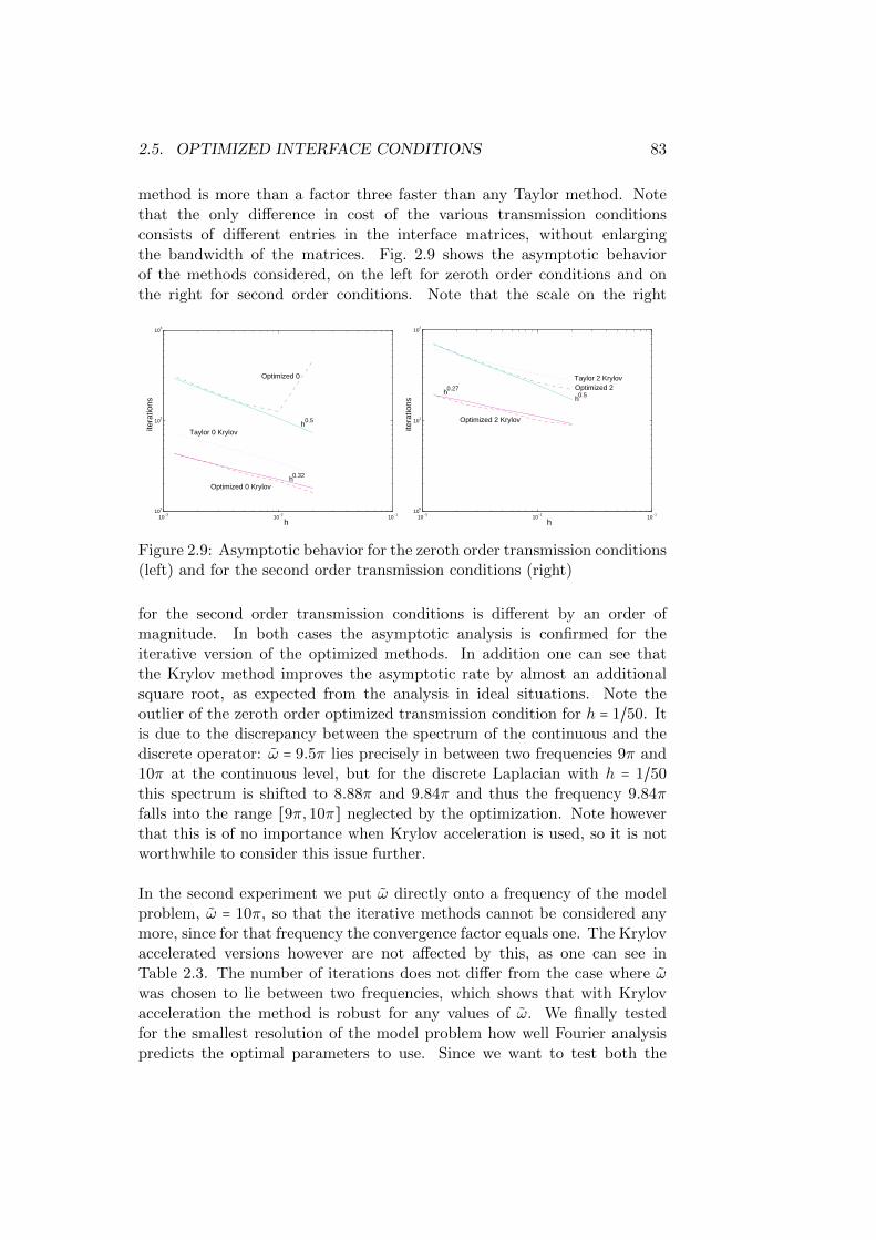
2.5. OPTIMIZED INTERFACE CONDITIONS 83
method is more than a factor three faster than any Taylor method. Notethat the only difference in cost of the various transmission conditionsconsists of different entries in the interface matrices, without enlargingthe bandwidth of the matrices. Fig. 2.9 shows the asymptotic behaviorof the methods considered, on the left for zeroth order conditions and onthe right for second order conditions. Note that the scale on the right
10−3
10−2
10−1
101
102
103
h
itera
tions
Taylor 0 Krylov
Optimized 0
Optimized 0 Krylov
h0.5
h0.32
10−3
10−2
10−1
100
101
102
h
itera
tions
Taylor 2 Krylov Optimized 2
Optimized 2 Krylov
h0.5h0.27
Figure 2.9: Asymptotic behavior for the zeroth order transmission conditions(left) and for the second order transmission conditions (right)
for the second order transmission conditions is different by an order ofmagnitude. In both cases the asymptotic analysis is confirmed for theiterative version of the optimized methods. In addition one can see thatthe Krylov method improves the asymptotic rate by almost an additionalsquare root, as expected from the analysis in ideal situations. Note theoutlier of the zeroth order optimized transmission condition for h = 1/50. Itis due to the discrepancy between the spectrum of the continuous and thediscrete operator: ω = 9.5π lies precisely in between two frequencies 9π and10π at the continuous level, but for the discrete Laplacian with h = 1/50this spectrum is shifted to 8.88π and 9.84π and thus the frequency 9.84πfalls into the range [9π,10π] neglected by the optimization. Note howeverthat this is of no importance when Krylov acceleration is used, so it is notworthwhile to consider this issue further.
In the second experiment we put ω directly onto a frequency of the modelproblem, ω = 10π, so that the iterative methods cannot be considered anymore, since for that frequency the convergence factor equals one. The Krylovaccelerated versions however are not affected by this, as one can see inTable 2.3. The number of iterations does not differ from the case where ωwas chosen to lie between two frequencies, which shows that with Krylovacceleration the method is robust for any values of ω. We finally testedfor the smallest resolution of the model problem how well Fourier analysispredicts the optimal parameters to use. Since we want to test both the

84 CHAPTER 2. OPTIMIZED SCHWARZ METHODS (OSM)
Order Zero Order Twoh Taylor Optimized Taylor Optimized
1/50 24 15 27 91/100 35 21 35 111/200 44 26 41 131/400 56 33 52 161/800 73 43 65 20
Table 2.3: Number of iterations for different transmission conditions anddifferent mesh parameter for the model problem when ω lies precisely on afrequency of the problem and thus Krylov acceleration is mandatory
iterative and the Krylov versions, we need to put again the frequency ωin between two problem frequencies, and in this case it is important to beprecise. We therefore choose ω to be exactly between two frequencies ofthe discrete problem, ω = 9.3596π, and optimized using ω− = 8.8806π andω+ = 9.8363π. Fig. 2.10 shows the number of iterations the algorithm needsto achieve a residual of 10e−6 as a function of the optimization parameters pand q of the zeroth order transmission conditions, on the left in the iterativeversion and on the right for the Krylov accelerated version. The Fourier
10 15 20 25 30 35 40 45 5010
15
20
25
30
35
40
45
50
q
p
35
35
40
40
40
4045
45
45
45
45
50
50
5050
50
50
50
55
55
55
55
55
55
55
60
60
60
60
60
60
60
65
65
65
65
65 65
65
70
70
70
70
70
10 15 20 25 30 35 40 45 5010
15
20
25
30
35
40
45
50
q
p
17
17
17
17
17
18
18
18
18
18
19
19
19
1919
20
20
20
2020
21
21
21
21
22
22
23
2425
Figure 2.10: Number of iterations needed to achieve a certain precision asfunction of the optimization parameters p and q in the zeroth order trans-mission conditions, for the iterative algorithm (left) and for the Krylov ac-celerated algorithm (right). The star denotes the optimized parameters p∗
and q∗ found by our Fourier analysis
analysis shows well where the optimal parameters lie and when a Krylovmethod is used, the optimized Schwarz method is very robust with respectto the choice of the optimization parameter. The same holds also for thesecond order transmission conditions, as Fig. 2.11 shows.

2.5. OPTIMIZED INTERFACE CONDITIONS 85
5 10 15 20 25 30 35 40 45 50 55 605
10
15
20
25
30
beta
alph
a
17
17
18
18
18
18
19
19
19
19
19
20
20
20 20
20
20
21
21
21
21
21
212222
22 2222
22
22
2424
24 24
24
24
24
26
26
26 26
26
26
26
28
28
28 2828
28
3030
30 30 30
3535
35 3535
4040
40 4040
4545
45 4545
45
5050
50
50
50
50
5555
55
55
55
55
6060
60
60
60
65
65
6570
7075 7580 85905 10 15 20 25 30 35 40 45 50 55 60
5
10
15
20
25
30
beta
alph
a
10
10
10
10
10
101111
11
11
11
1212
12
1212
1313
13
14
14
14
15
15
1516
1617
181920
Figure 2.11: Number of iterations needed to achieve a certain precisionas function of the optimization parameters α and β in the second ordertransmission conditions, for the iterative algorithm (left) and for the Krylovaccelerated algorithm (right). The star denotes the optimized parametersα∗ and β∗ found by our Fourier analysis
Noise levels in a VOLVO S90
We analyze the noise level distribution in the passenger cabin of a VOLVOS90. The vibrations are stemming from the part of the car called firewall.This example is representative for a large class of industrial problems whereone tries to determine the acoustic response in the interior of a cavity causedby vibrating parts. We perform a two dimensional simulation on a verti-cal cross section of the car. Fig. 2.12 shows the decomposition of the carinto 16 subdomains. The computations were performed in parallel on a net-work of sun workstations with 4 processors. The problem is characterized
12
12 4 3 513
915
117
1610
14 6
8
Figure 2.12: Decomposition into 16 subdomains (left) and acoustic field inthe passenger compartment (right) of the VOLVO S90
by ωa = 18.46 which corresponds to a frequency of 1000 Hz in the car oflength a. To solve the problem, the optimized Schwarz method was used asa preconditioner for the Krylov method ORTHODIR, and as convergence

86 CHAPTER 2. OPTIMIZED SCHWARZ METHODS (OSM)
criterion we used
∥Ku − f∥L2 ≤ 10−6∥f∥L2 . (2.91)
When using zeroth order Taylor conditions and a decomposition into16 subdomains, the method needed 105 iterations to converge, whereaswhen using second order optimized transmission conditions, the methodconverged in 34 iterations, confirming that also in real applications theoptimized Schwarz method is about a factor 3 faster, as we found for themodel problem earlier. Fig. 2.12 shows the acoustic field obtained in thepassenger compartment of the VOLVO S90.
2.5.3 Optimized conditions for other equations
Over the last years, a lot of results have been obtained for different classes ofequations and optimized algorithms based on carefully chosen parameters inthe transmission conditions, have been derived. For steady state symmetricproblems, we can cite [42, 86]. For advection-diffusion type problems, see[115, 113, 114, 130, 143, 144]. As far as the Helmholtz equations are con-cerned, optimized transmission conditions were developed in [27, 28, 34, 91,89]. There are also works for problems involving discontinuous coefficientsin [67, 82, 96]. Other particular aspects has been discussed, such as theinfluence of the geometry [85], coarse grid corrections [68], cross points[90] or circular domains [93]. In fluid dynamics, optimized transmissionconditions have been studied in [56, 54, 55]. See also [187] for porousflow media. Like the Helmholtz equations, high-frequency time-harmonicMaxwell’s equations are difficult to solve by classical iterative methodssince they are indefinite in nature. Optimized methods have been developedboth for the first order formulation of Maxwell equations in [57, 58, 53] or[72, 73] and also for the second order formulation in [27][section 4.7], [33, 4,163, 162, 166].
All the previous methods were based on optimized polynomial approxima-tions of the symbol of the transparent boundary conditions. An alternativeis the use of the rational approximations of Pade type, see [6]. Perfectlymatched layers (PML) [119] [29] are also used in domain decompositionmethods [171], [6]. Note as well that approximate factorization methodsfor the Helmholtz operator can be designed using absorbing boundaryconditions [92] or PML [164]. For applications to real life problems usinga Discontinuous Galerkin method can be found in [57, 58, 74]. For finite-element based non-overlapping and non-conforming domain decompositionmethods for the computation of multiscale electromagnetic radiation andscattering problems we refer to [126, 163, 162, 166]. In a recent workthe first order and second order formulations were presented in a unified

2.6. FREEFEM++ IMPLEMENTATION OF ORAS 87
framework in [52, 51].
Note that the method of deriving optimized transmission conditions is quitegeneral and can be in principle applied to other types of equations.
2.6 FreeFem++ implementation of ORAS
As a numerical illustration, we solve the Helmholtz equation in a square Ωof size 6 wavelengths with first order absorbing boundary condition:
−k2u −∆u = f in Ω ,∂u
∂n+ iku = 0 on ∂Ω .
The right handside f is a Gaussian function. The real part of the solu-tion is plotted on Figure 2.13. After discretization, the resulting linear
Figure 2.13: Real part of a solution of a Helmholtz equation
system (2.49) is solved by a domain decomposition method. As explainedin chapter 3, it is more profitable to use a Krylov method preconditionedby the ORAS operator M−1
ORAS (2.53) in place of the iterative fixed-pointalgorithm (2.22). We solve (2.49) by a preconditioned GMRES. We needto provide the FreeFem++ implementation for the ORAS preconditioner.As in the case of the Schwarz algorithm, we need to create a specific datafile dataHelmholtz.edp and a partition of unity and the restriction andextension operators.

88 CHAPTER 2. OPTIMIZED SCHWARZ METHODS (OSM)
load ”metis”load ”medit”
3 int nn=4,mm=4; // number of the domains in each directionint npart= nn∗mm; // total number of domainsint nloc = 40; // local no of dof per domain in one directionbool withmetis = 0; // =1 (Metis decomp) =0 (uniform decomp)
7 int sizeovr = 2; // size of the overlapreal allong = real(nn)/real(mm); // aspect ratio of the global domain// Mesh of a rectangular domainmesh Th=square(nn∗nloc,mm∗nloc,[x∗allong,y]);
11 fespace Vh(Th,P1);fespace Ph(Th,P0);Ph part; // piecewise constant functionint[int] lpart(Ph.ndof); // giving the decomposition
15 // Domain decomposition data structuresmesh[int] aTh(npart); // sequence of ovr. meshesmatrix[int] Rihreal(npart); // local restriction operatorsmatrix[int] Dihreal(npart); // partition of unity operators
19 matrix<complex>[int] Rih(npart); // local restriction operatorsmatrix<complex>[int] Dih(npart); // partition of unity operatorsint[int] Ndeg(npart); // number of dof for each meshreal[int] AreaThi(npart); // area of each subdomain
23 matrix<complex>[int] aA(npart); // local Dirichlet matricesmatrix<complex>[int] aR(npart); // local Robin matrices// Definition of the problem to solve// −kˆ2∗u − Delta (u) = f,
27 // u = g, Dirichlet boundary (top and bottom)// dn(u) + i k u = 0, Robin boundary (left and right)int Dirichlet=1, Robin=2;int[int] chlab=[1, Robin, 2, Robin, 3, Robin, 4, Robin];
31 Th=change(Th,refe=chlab);macro Grad(u) [dx(u),dy(u)] // EOMreal k=12.∗pi;func f = exp(−((x−.5)ˆ2+(y−.5)ˆ2)∗120.);//1; // right hand side
35 func g = 0; // Dirichlet datavarf vaglobal(u,v) = int2d(Th)(−kˆ2∗u∗v+Grad(u)’∗Grad(v))
+ int1d(Th,Robin)(1i∗k∗u∗v) − int2d(Th)(f∗v)+ ⤸Ç on(Dirichlet,u=g) ;
matrix<complex> Aglobal;39 Vh<complex> rhsglobal,uglob; // rhs and solution of the global problem
complex alpha = 1i∗k; // Despres algorithm// Optimal alpha:// h12: the mesh size for a rectangular domain of dimension 2x1,
43 // that is obtained with nnxmm = 2x1,4x2,8x4real h21 = 1./(mm∗nloc);real kplus = k+pi/1; // the rectangle height is 1real kminus = k−pi/1;
47 real Cw = min(kplusˆ2−kˆ2,kˆ2−kminusˆ2);real alphaOptR = pow(Cw/h21,1/3.)/2;complex alphaOpt = alphaOptR + 1i∗alphaOptR;//alpha = alphaOpt;
51 //alpha=1.0e30;// Iterative solverreal tol=1e−4; // tolerance for the iterative methodint maxit=1000; // maximum number of iterations
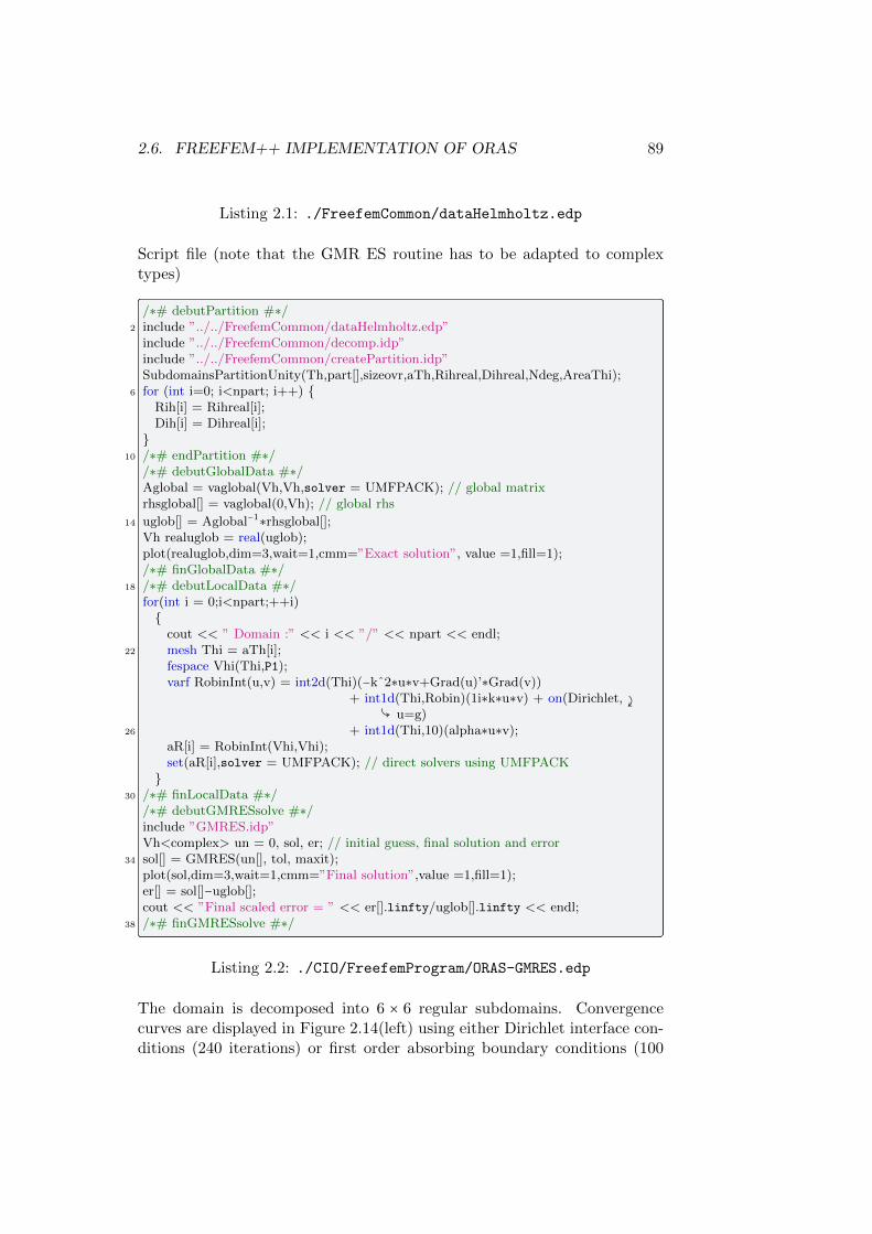
2.6. FREEFEM++ IMPLEMENTATION OF ORAS 89
Listing 2.1: ./FreefemCommon/dataHelmholtz.edp
Script file (note that the GMR ES routine has to be adapted to complextypes)
/∗# debutPartition #∗/2 include ”../../FreefemCommon/dataHelmholtz.edp”
include ”../../FreefemCommon/decomp.idp”include ”../../FreefemCommon/createPartition.idp”SubdomainsPartitionUnity(Th,part[],sizeovr,aTh,Rihreal,Dihreal,Ndeg,AreaThi);
6 for (int i=0; i<npart; i++) Rih[i] = Rihreal[i];Dih[i] = Dihreal[i];
10 /∗# endPartition #∗/
/∗# debutGlobalData #∗/Aglobal = vaglobal(Vh,Vh,solver = UMFPACK); // global matrixrhsglobal[] = vaglobal(0,Vh); // global rhs
14 uglob[] = Aglobal−1∗rhsglobal[];Vh realuglob = real(uglob);plot(realuglob,dim=3,wait=1,cmm=”Exact solution”, value =1,fill=1);/∗# finGlobalData #∗/
18 /∗# debutLocalData #∗/for(int i = 0;i<npart;++i)
cout << ” Domain :” << i << ”/” << npart << endl;22 mesh Thi = aTh[i];
fespace Vhi(Thi,P1);varf RobinInt(u,v) = int2d(Thi)(−kˆ2∗u∗v+Grad(u)’∗Grad(v))
+ int1d(Thi,Robin)(1i∗k∗u∗v) + on(Dirichlet, ⤸Ç u=g)
26 + int1d(Thi,10)(alpha∗u∗v);aR[i] = RobinInt(Vhi,Vhi);set(aR[i],solver = UMFPACK); // direct solvers using UMFPACK
30 /∗# finLocalData #∗/
/∗# debutGMRESsolve #∗/include ”GMRES.idp”Vh<complex> un = 0, sol, er; // initial guess, final solution and error
34 sol[] = GMRES(un[], tol, maxit);plot(sol,dim=3,wait=1,cmm=”Final solution”,value =1,fill=1);er[] = sol[]−uglob[];cout << ”Final scaled error = ” << er[].linfty/uglob[].linfty << endl;
38 /∗# finGMRESsolve #∗/
Listing 2.2: ./CIO/FreefemProgram/ORAS-GMRES.edp
The domain is decomposed into 6 × 6 regular subdomains. Convergencecurves are displayed in Figure 2.14(left) using either Dirichlet interface con-ditions (240 iterations) or first order absorbing boundary conditions (100

90 CHAPTER 2. OPTIMIZED SCHWARZ METHODS (OSM)
iterations). These results are obtained by a one level method that is with-out a coarse space correction. We can improve them by adding a speciallydesigned coarse space for Helmholtz equations [36]. The effect can be seen inFigure 2.14 (right). We plot the convergence curves for the one level Despresalgorithm and its acceleration using either 5 or 10 vectors per subdomain inthe coarse space.
0 50 100 150 200 25010−4
10−3
10−2
10−1
100
101
Iterations
Res
idua
l
DirichletDespres
0 10 20 30 40 50 60 70 80 90 10010−4
10−3
10−2
10−1
100
Iterations
Res
idua
l
DespresCS−5CS−10
Figure 2.14: Left: Comparison between Schwarz and Despres algorithms.Right: Comparison between one level Despres algorithm and its accelerationwith a coarse space [36]

Chapter 3
Krylov methods
In chapter 1, we introduced Schwarz methods as iterative solvers. Theaim of this chapter is to explain the benefit of using domain decompositionmethods as preconditioners for Krylov type methods such as CG (conjugategradient), GMRES or BICGSTAB. In § 3.1, we present fixed point methods.In § 3.2, we introduce the fundamental notion of Krylov subspace. Thisyields to two celebrated algorithms: the Conjugate Gradient (CG) methodfor symmetric positive definite problems § 3.3 and the Generalized MinimalRESidual (GMRES) method for nonsymmetric linear systems § 3.4. At theend of § 3.4, we explain why Krylov methods are always preferable to fixedpoint iterations. In § 3.5, the case where the system is not invertible isdealt with. Finally, in § 3.6, we give FreeFem++ implementations and useof Krylov methods for domain decomposition methods. It should be noticedthat the detailed and sometime technical derivation of these methods is notnecessary for using them with success.3.6
Recall first that the iterative versions of the Schwarz methods introduced inchapter 1 can be written as preconditioned fixed point iterations
Un+1 = Un +M−1rn, rn ∶= F −AUn
where M−1 is depending on the method used (RAS or ASM). The key pointin what follows is to prove that fixed point methods (3.3) are intrinsicallyslower than Krylov methods, for more details see [41]. Since this result isvalid for any fixed point method, we will start by placing ourselves in anabstract linear algebra framework and then apply the results to the Schwarzmethods.
3.1 Fixed point iterations
Consider the following well-posed but difficult to solve linear system
Ax = b, x ∈ RN (3.1)
91
92 CHAPTER 3. KRYLOV METHODS
and M an “easy to invert” matrix of the same size than A. Actually byeasy to invert, we mean that the matrix-vector of M−1 by a residual vectorr = b − Ax is cheap. Then, equation (3.1) can be solved by an iterativemethod
M xn+1 =M xn + (b −Axn)⇔M xn+1 =M xn + rn . (3.2)
This suggests the following definition.
Definition 3.1.1 (Fixed point method) The following algorithm equiv-alent to (3.2)
xn+1 = xn +M−1(b −Axn)⇔ xn+1 = xn +M−1rn (3.3)
is called a fixed point algorithm and the solution x of (3.1) is a fixed pointof the operator:
xz→ x +M−1(b −Ax) .The difference between matrices A and M is denoted by P ∶=M −A. Whenconvergent the iteration (3.3) will converge to the solution of the precondi-tioned system
M−1Ax =M−1b .
The above system which has the same solution as the original system iscalled a preconditioned system; here M−1 is called the preconditioner. Inother words, a splitting method is equivalent to a fixed-point iteration on apreconditioned system. We see that the fixed point iterations (3.3) can bewritten as
xn+1 = xn +M−1(b −Axn)
= (I −M−1(M − P ))xn +M−1b
= M−1Pxn +M−1b
= M−1Pxn +M−1Ax =M−1Pxn +M−1(M − P )x
= x +M−1P (xn − x) .
(3.4)
From (3.4) it is easy to see that the error vector en ∶= xn − x verifies
en+1 =M−1Pen
so thaten+1 = (M−1P )n+1e0. (3.5)
For this reason M−1P is called the iteration matrix associated with (3.4)and since the expression of the iteration doesn’t change w.r.t. to n, we call(3.4) a stationary iteration.We recall below the well-known convergence results in the case of stationaryiterations.

3.2. KRYLOV SPACES 93
Lemma 3.1.1 (Convergence of the fixed point iterations) The fixedpoint iteration (3.4) converges for arbitrary initial error e0 (that is en → 0as n→∞) if and only if the spectral radius of the iteration matrix is inferiorto 1, that is ρ(M−1P ) < 1 where
ρ(B) = max∣λ∣, λ eigenvalue of B.
For the detailed proof see for example [103].
In general, it is not easy to ensure that the spectral radius of the iterationmatrix M−1P is smaller than one. Except for M -matrices (A non-singularand A−1 non-negative), for which any regular splitting A = M − P (Mnon-singular, M−1 and P non-negative) leads to a convergent fixed pointiteration. (see Chapter 4 in [169] for details).
These drawbacks of fixed point methods motivate the use of Krylov typemethods which are much more efficient in terms of robustness and speed.
3.2 Krylov spaces
In this section we will show that the solution of a fixed point method belongsto an affine space called Krylov space. We start by showing that the solutionof a fixed point iteration can be written as a series.
Lemma 3.2.1 (Fixed point solution as a series) Let
zn ∶=M−1rn =M−1(b −Axn)
be the residual preconditioned by M at the iteration n for the fixed pointiteration
xn+1 = xn + zn = xn +M−1(b −Axn) (3.6)
Then, the fixed point iteration is equivalent to
xn+1 = x0 +n
∑i=0
(M−1P )i z0 . (3.7)
Proof Note that we have that
xn+1 = xn +M−1rn = xn + zn ⇒ xn+1 = x0 + z0 + z1 +⋯ + zn. (3.8)
From (3.5) we see that the residual vector rn = b−Axn = −A(xn−x) verifies
rn = −Aen = (P −M)(M−1P )ne0 = (PM−1)nPe0 − (PM−1)n−1Pe0
= (PM−1)n(Pe0 −Me0) = (PM−1)nr0.(3.9)

94 CHAPTER 3. KRYLOV METHODS
From (3.9) we have that
zn =M−1rn =M−1(PM−1)nr0 =M−1(PM−1)nMz0 = (M−1P )nz0. (3.10)
From (3.8) and (3.10) we obtain
xn+1 = x0 + z0 + (M−1P )z1 +⋯ + (M−1P )nzn = x0 +n−1
∑i=0
(M−1P )i z0. (3.11)
which leads to the conclusion. Thus the error xn+1 −x0 is a geometric seriesof common ratio M−1P . Note that (3.11) can be also written in terms ofthe residual vector.
xn+1 = x0 +M−1r0 + (M−1P )M−1r1 +⋯ + (M−1P )nM−1rn
= x0 +n−1
∑i=0
(M−1P )iM−1 r0.(3.12)
The previous result leads to the following remark.
Remark 3.2.1 The correction xn+1 − x0 is given by
xn+1 − x0 = Sn(M−1P )M−1 r0 = Sn(M−1P )z0 , (3.13)
where Sn is the polynomial given by Sn(t) = 1 + t + ⋯ + tn. Moreover, from(3.12) we see that
xn+1 − x0 ∈ SpanM−1r0, (M−1P )M−1r0,⋯, (M−1P )nM−1r0
= Spanz0, (M−1P )z0,⋯, (M−1P )nz0(3.14)
In conclusion the solution of a fixed point iteration is generated in a spacespanned by powers of the iteration matrix M−1P = I −M−1A applied to agiven vector. The main computational cost is thus given by the multiplica-tion by the matrix A and by the application of M−1. At nearly the samecost, we could generate better approximations in the same space (or betterpolynomials of matrices).
Definition 3.2.1 (Krylov spaces) For a given matrix B and a vector ywe define the Krylov subspaces of dimension n associated to B and y by
Kn(B,y) ∶= Spany, By, . . . ,Bn−1y .
Therefore, a Krylov space is a space of polynomials of a matrix times avector.

3.2. KRYLOV SPACES 95
According to the previous definition, we see from (3.14) that
xn − x0 ∈ Kn(M−1P,M−1r0) = Kn(M−1P,z0).By the same kind of reasoning, we also have that
en = (M−1P )ne0 ⇒ en ∈ Kn+1(M−1P,e0),
zn = (M−1P )nz0 ⇒ zn ∈ Kn+1(M−1P,z0).But since M−1P = I −M−1A we see that
Kn(M−1P,z0) = Kn(M−1A,z0).A reasonable way to compute iteratively a solution would be to look foran optimal element in the above mentioned space. This element will benecessarily better and will approach faster the solution than a fixed pointmethod. Krylov type methods differ by the way an “optimality” conditionis imposed in order to uniquely define xn and by the actual algorithm thatimplements it.
Remark 3.2.2 Note also that the difference between two successive iteratesis given by
xn+1 − xn = (M−1P )zn = (M−1P )nM−1r0
= (I −M−1A)nM−1r0 ∈ Kn+1(M−1A,M−1r0)This sequence can be further improved by searching for a better solution inthis Krylov space.
Example 3.2.1 From the family of fixed point methods we can mention theRichardson iterations with a relaxation parameter.
xn+1 = xn + αrn = xn + α(b −Axn). (3.15)
The parameter α can be chosen in such a way to have the best convergencefactor over the iterations. In the case of a symmetric positive definite matrix,the value of α which minimizes the convergence rate of the algorithm is
αopt =2
λmin(A) + λmax(A)and in this case the error behaves as
∥en∥A ≤ (κ2(A) − 1
κ2(A) + 1)n
∥e0∥A
where
κ2(A) = λmax(A)λmin(A)
is the condition number of A, λmax(A) and λmin(A) being the extreme eigen-values of A. In practice, it is very difficult to estimate accurately λmin orλmax and thus αopt. This motivates the introduction of the gradient methodin the next paragraph.

96 CHAPTER 3. KRYLOV METHODS
3.2.1 Gradient methods
This suggests the definition of a new class of methods for symmetric positivematrices.
Definition 3.2.2 (Gradient methods) A descent method is an iterationof the form
xn+1 = xn + αnpn, αn ≥ 0 (3.16)
where αn is chosen such that it minimizes ∥en+1∥2A = ∥xn+1 − x∥2
A (thesquare of the A-norm for the error norm at each iteration, ∥en+1∥2
A ∶=(Aen+1, en+1)2) and vector pn is called the descent direction. If pn = rn,the resulting method is called optimal gradient method.
Consider function f :
α z→ f(α) ∶= ∥xn + αpn − x∥2A
and the minimization problem
f(αn) ∶= ∥xn + αnpn´¹¹¹¹¹¹¹¹¹¹¹¹¹¹¹¹¹¹¹¹¸¹¹¹¹¹¹¹¹¹¹¹¹¹¹¹¹¹¹¹¹¹¶
xn+1
−x∥2A
= minα
∥xn + αpn − x∥2A = min
α(A(xn + αpn − x),xn + αpn − x)
= minα
[α2(Apn,pn) + 2α(Apn,xn − x) + (A(xn − x),xn − x)]
= minα
[α2(Apn,pn) − 2α(pn,A(x − xn)´¹¹¹¹¹¹¹¹¹¹¹¹¹¹¹¹¹¹¹¹¸¹¹¹¹¹¹¹¹¹¹¹¹¹¹¹¹¹¹¹¹¶
rn
)] + (A(xn − x),xn − x).
We have that the optimal parameter αn is characterized by:
∂f
∂α(αn) = 0⇒ αn =
(pn, rn)(Apn,pn) . (3.17)
Note that in the case of the gradient method (pn = rn) αn becomes
αn =∥rn∥2
2
∥rn∥2A
= (en, rn)A∥rn∥2
A
. (3.18)
We have the following convergence result.
Lemma 3.2.2 (Optimal gradient convergence) The optimal step gra-dient method xn+1 = xn + αnrn, with αn chosen in (3.18) converges and theerror estimate is verifying the estimate
∥en∥A ≤ (1 − 1
κ2(A))n2
∥e0∥A
where κ2(A) = λmax(A)
λmin(A)is the condition number of A.

3.3. THE CONJUGATE GRADIENT METHOD 97
Proof From (3.16) we see that
∥en+1∥2A = ∥en + αnrn∥2
A = ∥en∥2A + 2αn (en, rn)A
´¹¹¹¹¹¹¹¹¹¹¹¹¹¹¹¹¸¹¹¹¹¹¹¹¹¹¹¹¹¹¹¹¹¹¶−αn∥rn∥2
A
+α2n∥rn∥2
A
= ∥en∥2A − α2
n∥rn∥2A = ∥en∥2
A − α2n(Arn, rn) = ∥en∥2
A −(rn, rn)2
(Arn, rn)= ∥en∥2
A (1 − (rn, rn)(A−1rn, rn) ⋅
(rn, rn)(Arn, rn)) ,
where we have used the identity:
∥en∥2A = (en,Aen) = (A−1rn, rn) .
Matrix A being symmetric positive definite we have
λmin(A) ≤ (rn, rn)(A−1rn, rn) ≤ λmax(A) and
1
λmax(A) ≤ (rn, rn)(Arn, rn) ≤ 1
λmin(A)which leads to the estimate
∥en+1∥2A ≤ (1 − λmin(A)
λmax(A)) ∥en∥2A ⇒ ∥en∥A ≤ (1 − 1
κ2(A))n2
∥e0∥A
and this ends the proof.
3.3 The Conjugate Gradient method
We present here a Krylov method that applies to symmetric positive definite(SPD) matrices. Suppose that we want to solve Ax = b with A a SPDmatrix. The idea is that the solution at each iteration solves a minimizationproblem in the A-norm over a Krylov space:
Find yn ∈ Kn(A, r0) such that
∥en∥A = ∥x − (x0 + yn)´¹¹¹¹¹¹¹¹¹¹¹¹¹¹¹¹¹¸¹¹¹¹¹¹¹¹¹¹¹¹¹¹¹¹¹¹¶
xn
∥A = minw∈Kn(A,r0)
∥x − (x0 +w)∥A . (3.19)
In the following we will define a new method that extends the idea of gradientmethods and will prove afterwards that is exactly the Krylov method whoseiterates are given by (3.19).
Definition 3.3.1 (Conjugate Gradient) Starting from an initial guessx0 and an initial descent direction p0 = r0 = b −Ax0, a conjugate gradientmethod is an iteration of the form
xn+1 = xn + αnpn,
rn+1 = rn − αnApn,
pn+1 = rn+1 + βn+1pn,
(3.20)

98 CHAPTER 3. KRYLOV METHODS
where αn and βn are chosen such that they minimize the norm of the error∥en+1∥2
A = ∥xn+1 − x∥2A at each iteration.
Coefficients αn and βn+1 are easy to find. First, from (3.18) we see that thecoefficient αn which minimizes ∥en+1∥2
A is necessarily given by
αn =(pn, rn)
(Apn,pn) . (3.21)
By taking the dot product of the second relation of (3.20) by pn and byusing (3.21) into it, we see that
(rn+1,pn) = (rn,pn) − αn(Apn,pn) = 0.
By taking the dot product of the third relation of (3.20) by rn+1 and byusing the previous orthogonality relation we obtain
(pn+1, rn+1) = (rn+1, rn+1) + βn+1(rn+1,pn) = (rn+1, rn+1), ∀n ≥ 0.
By replacing the last relation taken in n into (3.21) we get
αn =(rn, rn)
(Apn,pn) = ∥rn∥22
∥pn∥2A
. (3.22)
In a similar way we can find βn+1. If we replace the (3.22) taken in n + 1into ∥en+2∥2
A and use the third relation of (3.20) to replace pn+1 we get
∥en+2∥2A = ∥xn+2 − x∥2
A = ∥xn+1 − x + αn+1pn+1∥2
A
= ∥en+1∥2A + 2(Aen+1
´¹¹¹¹¸¹¹¹¹¹¶−rn+1
, αn+1pn+1) + α2
n+1∥pn+1∥2A
= ∥en+1∥2A − 2αn+1(rn+1, rn+1) + α2
n+1∥pn+1∥2A
= ∥en+1∥2A −
(rn+1, rn+1)4
(Apn+1,pn+1)= ∥en+1∥2
A −(rn+1, rn+1)4
(A(rn+1 + βn+1pn), (rn+1 + βn+1pn)).
Therefore, minimizing ∥en+2∥2A with respect to βn+1 is equivalent to mini-
mizing the quadratic form (A(rn+1 +βn+1pn), (rn+1 +βn+1p
n)) with respectto βn+1, which gives
βn+1 = −(Arn+1,pn)(Apn,pn) . (3.23)
By taking the A-dot product of the third relation of (3.20) by pn and byusing (3.23) into it see that
(Apn+1,pn) = (Arn+1,pn) + βn+1(Apn,pn) = 0 .

3.3. THE CONJUGATE GRADIENT METHOD 99
Using this identity and taking the A-dot product of the third relation of(3.20) by pn+1 we get
(Apn+1,pn+1) = (Arn+1,pn+1) + βn(Apn+1,pn)= (Arn+1,pn+1) = (Apn+1, rn+1) (3.24)
By using (3.24) into the dot product of the second relation of (3.20) by rn
(rn+1, rn) = (rn, rn) − αn(Apn, rn) = (rn, rn) − αn(Apn,pn) = 0. (3.25)
Finally by taking the dot product of the second relation of (3.20) by rn+1
and by using (3.25)
(rn+1,Apn) = −∥rn+1∥22
αn. (3.26)
By plugging (3.26) into (3.23) we conclude by using the expression of (3.22)that
βn+1 =∥rn+1∥2
2
∥rn∥22
. (3.27)
The resulting algorithm is given in Algorithm 4, see [9].
Algorithm 4 CG algorithm
Compute r0 ∶= b −Ax0, p0 = r0
for i = 0,1, . . . doρi = (ri, ri)2
qi = Apiαi =
ρi(pi,qi)2
xi+1 = xi + αipiri+1 = ri − αiqiρi+1 = (ri+1, ri+1)2
βi+1 =ρi+1
ρipi+1 = ri+1 + βi+1picheck convergence; continue if necessary
end for
We can see that the conjugate gradient algorithm has a few remarkableproperties that can be stated in the following lemma.
Lemma 3.3.1 (Conjugate Gradient as a Krylov method) Thedescent directions pn are A-orthogonal or conjugate
(Apk,pl) = 0, ∀k, l, k ≠ l
and the residual vectors are orthogonal between them and to the descentdirections
(rk, rl) = 0, ∀k, l, k ≠ l and (pk, rl) = 0, ∀k, l, k < l

100 CHAPTER 3. KRYLOV METHODS
Moreover, both the descent directions and the residuals span the Krylovspace:
Kn+1(A, r0) = Spanr0, r1,⋯, rn = Spanp0,p1,⋯,pn (3.28)
and vector xn from (3.20) minimizes the error norm ∥en∥2A on the affine
space x0 +Kn(A, r0). The algorithm will converge in at most N iterations,N being the size of matrix A.
Proof The proof is a direct consequence of the algebraic manipulationsperformed previously to find the coefficients αn and βn+1. The property(3.28) can be obtained by recurrence on the relations (3.20) and in thesame way the fact that xn ∈ x0 +Kn(A, r0). Moreover, the matrix A beingsymmetric positive definite, there exists an A-orthogonal basis of size N ,which explains why we cannot have more than N conjugate descent vectors.This leads to a convergence in at most N iterations.
Lemma 3.3.2 (Convergence of the Conjugate Gradient method)The conjugate gradient method defined in (3.20) converges to the solutionof the linear system Ax = b and we have the error estimate:
∥en∥A ≤ 2⎛⎝
√κ2(A) − 1
√κ2(A) + 1
⎞⎠
n
∥e0∥A (3.29)
where κ2(A) is the condition number of the matrix A.
Proof As we have seen previously, the conjugate gradient method is aKrylov method. Since
en ∈ Kn(A, r0) = Kn+1(A,e0)
this means that building a sequence of iterates xn is equivalent to build asequence of polynomials Pn ∈ Pn with real coefficients such that
• en = Pn(A)e0.
• Pn(0) = 1.
• Pn minimizes J(Q) = ∥Q(A)e0∥2A over all the polynomials Q ∈ Pn such
that Q(0) = 1.
Matrix A can be diagonalized using orthonormal eigenvectors A = TΛT t.For any given polynomial Q,
Q(A) = TQ(Λ)T t.
3.3. THE CONJUGATE GRADIENT METHOD 101
Therefore we have for any monic (coefficient of the leading term is equal toone) polynomial Q of degree n
∥en∥A = ∥Pn(A)e0∥A ≤ ∥Q(A)e0∥A = ∥TQ(Λ)T te0∥A ≤ maxλ∈σ(A)
∣Q(λ)∣∥e0∥A
and the estimate yields
∥en∥A ≤ minQ∈Pn,Q(0)=1
maxλ∈[λ1,λ2]
∣Q(λ)∣∥e0∥A, (3.30)
where λ1 = λmin(A) and λ2 = λmax(A). We know from [25] that
maxx∈[λ1,λ2]
Q∗(x) = minQ∈Pn,Q(0)=1
maxx∈[λ1,λ2]
∣Q(x)∣,
where
Q∗(x) =Tn (2x−λ1−λ2
λ2−λ1)
Tn (−λ1−λ2
λ2−λ1),
with Tn being the Chebyshev polynomial of the first kind
Tn(x) =⎧⎪⎪⎪⎨⎪⎪⎪⎩
(x +√x2 − 1)n + (x −
√x2 − 1)n
2, ∣x∣ > 1,
cos(narccos(x)) , ∣x∣ ≤ 1.
We see that
maxx∈[λ1,λ2]
∣Q∗(x)∣ = 1
∣Tn (−λ1−λ2
λ2−λ1)∣
= 1
Tn (κ2(A)+1κ2(A)−1)
= 2
(√κ2(A)−1
√κ2(A)+1
)−n
+ (√κ2(A)−1
√κ2(A)+1
)n ≤ 2
⎛⎝
√κ2(A) − 1
√κ2(A) + 1
⎞⎠
n
(3.31)From (3.31) and (3.30) the conclusion follows.
Remark 3.3.1 We estimate the iteration counts to reach a reduction factorof the error by a factor ε ≪ 1 for a poorly conditioned system, κ2(A) ≫1. From Lemma 3.2.2, the optimal gradient method will converge in nOGiterations with :
ε = (1 − 1
κ2(A))nOG
2
.
Thus, we have
log ε = nOG2
log(1 − 1
κ2(A)) ,

102 CHAPTER 3. KRYLOV METHODS
that isnOG ≃ 2κ2(A) (− log ε) .
From Lemma 3.3.2, the conjugate gradient method will converge in nCGiterations with:
nCG ≃√κ2(A)
2(− log ε) .
These estimates are clearly in favor of the CG algorithm over the optimalgradient method.
3.3.1 The Preconditioned Conjugate Gradient Method
In order to have a faster convergence, a SPD preconditioner denoted hereM is often used. In order to preserve the SPD properties, we use the factthat M−1 admits a SPD square root denoted M−1/2 such that
M−1/2 ⋅ M−1/2 =M−1 .
The CG method is applied to the symmetrized preconditioned system
(M−1/2AM−1/2)M1/2x =M−1/2 b.
instead of simply M−1A since the latter is generally non-symmetric, butits spectrum is the same as of matrix M−1/2AM−1/2. A naive and costlyimplementation would require the quite expensive computation of the squareroot of the inverse of operator M . Once again, a detailed analysis revealsthat it can be bypassed.
Lemma 3.3.3 (Preconditioned Conjugate Gradient) The conjugategradient method applied to the system
Ax = b, (3.32)
withA =M−1/2AM−1/2, x =M1/2x, b =M−1/2 b
can be rewritten as the following iterative method: starting from and initialguess x0 and of an initial descent direction
p0 =M−1r0 =M−1(b −Ax0),
compute the sequence of approximations as
xn+1 = xn + αnpn,
rn+1 = rn − αnApn,
pn+1 = M−1rn+1 + βn+1pn,
(3.33)

3.3. THE CONJUGATE GRADIENT METHOD 103
where αn and βn+1 are given by
αn =(M−1rn, rn)
∥pn∥2A
, βn+1 =(M−1rn+1, rn+1)
(M−1rn, rn) . (3.34)
Proof Suppose we apply now the conjugate gradient method (3.20) to thesystem (3.32). This gives
xn+1 = xn + αnpn,
rn+1 = rn − αnApn,
pn+1 = rn+1 + βn+1pn,
(3.35)
with
xn =M1/2xn, pn =M1/2pn, rn =M−1/2rn, A =M−1/2AM−1/2. (3.36)
and the coefficients
αn = (rn, rn)∥pn∥2
A
= (M−1/2rn,M−1/2rn)((M−1/2AM−1/2)M1/2pn,M1/2pn)
= (M−1rn, rn)∥pn∥2
A
,
βn = (rn+1, rn+1)(rn, rn) = (M−1/2rn+1,M−1/2rn+1)
(M−1/2rn,M−1/2rn)= (M−1rn+1, rn+1)
(M−1rn, rn)(3.37)
which are exactly the coefficients from (3.34).By replacing now (3.36) into the three relations of (3.35), we obtain theiterations (3.33). The initial descent direction p0 is derived from
p0 = r0 ⇔M1/2p0 =M−1/2r0 ⇔ p0 =M−1r0.
which ends the proof.
We have just proved the the preconditioned conjugate gradient requiresonly the application of the preconditioner M−1 and the computation ofM−1/2 is thus not required. Moreover, since the spectrum of M−1/2AM−1/2
and M−1A is the same, in the convergence estimate (3.29) we simply haveto replace κ2(A) by κ2(M−1A).
The resulting iterative procedure is given in Algorithm 5.
Remark 3.3.2 There is another way of deriving the preconditioned form ofthe Conjugate Gradient Method by noting that even if M−1A is not symmet-ric, it is self-adjoint for the M -inner product (recall that M is symmetricpositive definite), that is
(M−1Ax, y)M = (Ax, y) = (x,Ay) = (x,M(M−1A)y) = (x,M−1Ay)M ,

104 CHAPTER 3. KRYLOV METHODS
Algorithm 5 PCG algorithm
Compute r0 ∶= b −Ax0, z0 =M−1r0, p0 = z0.for i = 0,1, . . . doρi = (ri,zi)2
qi = Apiαi =
ρi(pi,qi)2
xi+1 = xi + αipiri+1 = ri − αiqizi+1 =M−1ri+1
ρi+1 = (ri+1,zi+1)2
βi+1 =ρi+1
ρipi+1 = zi+1 + βi+1picheck convergence; continue if necessary
end for
where (x, y)M ∶= (Mx,y). Therefore, an alternative is to replace the usualEuclidean inner product in the Conjugate Gradient algorithm by the M -innerproduct. This idea is considered by Saad (see Chapter 9 of [169] for details).
3.4 The GMRES method for non-symmetric prob-lems
If either operator A or preconditioner M is not symmetric positive definitepositive, PCG algorithm cannot be used. The bad news is that in theunsymmetric case there is no method with a fixed cost per iteration thatleads to an optimal choice for xn. In this case, two popular methods are theGMRES [170] and BICGSTAB [185]. With a left preconditioning, they areapplied to preconditioned system
M−1Ax =M−1b
These methods differ by the way they pick an approximation xn to thesolution x in the Krylov subspace Kn((M−1A),z0) with z0 = M−1r0 =M−1(b −Ax0) being the initial preconditioned residual.In order to fix the ideas we will concentrate on the solution of the unprecon-ditioned system Ax = b, in the preconditioned case A needs to be replacedby M−1A and b by M−1b.Note that it makes sense to minimize the residual, because the error is ingeneral unknown, and we can only directly minimize special norms of theerror. Moreover, the norm of the error is bounded by a constant times thenorm of the residual
∥en∥2 = ∥A−1rn∥2 ≤ ∥A−1∥∥rn∥2
3.4. THE GMRES METHOD FOR NON-SYMMETRIC PROBLEMS 105
and finally we can note that
∥rn∥2 = (Aen,Aen) = (A∗Aen,en) = ∥en∥2A∗A.
In what follows we will concentrate on the GMRES method by explainingin detail the principles on which it is based and some ideas about its conver-gence properties. Let us introduce first the general framework of a minimalresidual method.
Definition 3.4.1 (Minimal residual method) Given an initial iteratex0 and the initial residual r0 = b −Ax0, a minimal residual method appliedto a system Ax = b will build the iterates xn = x0 + yn where
yn ∈ Kn(A, r0) such that
∥rn∥2 = ∥r0 −Ayn∥2 = minw∈Kn(A,r0)
∥Aw − r0∥2 .(3.38)
We say that they minimize the euclidean norm of the residual.
We see from the previous definition that we look for the vector xn = x0 +yn
such that yn achieves the minimum of ∥r0 − Ay∥ over Kn(A, r0). If thedimension of Kn(A, r0) is n and v1,v2,⋯,vn is a basis of it, then we canlook for yn under the form
yn =n
∑j=1
yjvj .
If we denote the function to minimize by
f(y1, y2,⋯, yn) = ∥r0 −An
∑i=1
yivi∥2
2
= ∥r0 −n
∑i=1
yiAvi∥2
2
then the optimality conditions ∂f∂yi
= 0 translates into
n
∑j=1
(Avj ,Avi)yj = (r0,Avi). (3.39)
If V denotes the matrix containing the column vectors vj then (3.39) isequivalent to the system
(V ∗A∗AV )Yn = F where Yn = (y1, y2,⋯, yn)T . (3.40)
Note that the size of the system (3.40) increases with the number of itera-tions, which means the algorithmic complexity to compute the solution of(3.40) increases as the number of iterations becomes larger. On the otherside, if the basis of Kn(A, r0) has no particular structure then the system(3.40) can be too ill-conditioned. The GMRES method proposes a cheapsolution by building a special basis of the Krylov space which makes thesystem easy to solve.

106 CHAPTER 3. KRYLOV METHODS
3.4.1 The GMRES method
The idea of the GMRES method is to build an orthonormal basis of theKrylov space by using a Gram-Schmidt algorithm. That is,
Starting from v1 =r0
∥r0∥2,
Compute vn+1 =Avn −
n
∑i=1
(Avn,vi)vi
∥Avn −n
∑i=1
(Avn,vi)vi∥2
, n ≥ 1.(3.41)
Computing the Gram-Schmidt orthogonalisation of the basis of a Krylovspace is called Arnoldi method.Supposing that the recurrence from (3.41) is well-defined (that is the de-nominator is non-null), then it is equivalent to
Avn =n
∑i=1
(Avn,vi)vi + ∥Avn −n
∑i=1
(Avn,vi)vi∥2
vn+1 (3.42)
If we denote by Vn the unitary matrix (V ∗n Vn = In) having as columns the first
n already computed orthonormal vectors v1,⋯,vn, then Vn+1 is obtainedfrom Vn by adding the column vector vn+1. Thus equation (3.42) can bere-written as
AVn = Vn+1Hn, (3.43)
where the entries of the rectangular matrix Hn ∈Mn+1,n(C) are
(Hn)i,n = (Avn,vi), i ≤ n,
(Hn)n+1,n = ∥Avn −n
∑i=1
(Hn)i,nvi∥2
.(3.44)
Moreover, since (Hn)l,m = 0, l >m+1, we say that Hn is a upper Hessenbergmatrix. Note also that the matrix Hn+1 is obtained from Hn by adding acolumn given by the elements (Hn+1)i,n+1 from (3.44) and a line whose onlynon-zero element is (Hn+1)n+2,n+1.With these notations and by using (3.43) we see that the problem (3.40) isequivalent to finding Yn such that
V ∗n A
∗AVnYn = ∥r0∥[(A∗v1,v1), (A∗v1,v2),⋯, (A∗v1,vn)]T ⇔
H∗n V
∗n+1Vn+1
´¹¹¹¹¹¹¹¹¹¹¹¹¹¹¹¹¸¹¹¹¹¹¹¹¹¹¹¹¹¹¹¹¹¶In
HnYn = ∥r0∥ [(H∗
n)1,1, (H∗n)2,1⋯, (H∗
n)n,1]T
(3.45)and consequently
H∗nHnY
n = βH∗nη1,n+1, where β = ∥r0∥2 (3.46)

3.4. THE GMRES METHOD FOR NON-SYMMETRIC PROBLEMS 107
where η1,n+1 is the first column vector of the canonical basis of Rn+1. Solvingsuch a system is straightforward if one knows the QR decomposition of Hn
Hn = QnRn
with Qn being a unitary matrix of order n+ 1 and Rn and upper triangularmatrix of size (n + 1) × n where the last line is null. This factorization isquite easy to compute in the case of an upper Hessenberg matrix (since it“almost” upper triangular). Supposing that this factorization is availablethen (3.46) reduces to the system
R∗n (Q∗
nQn)´¹¹¹¹¹¹¹¹¹¹¹¹¸¹¹¹¹¹¹¹¹¹¹¹¹¹¶
In
RnYn = βR∗
nQ∗nη1,n+1 ⇔ R∗
nRnYn = βR∗
nQ∗nη1,n+1. (3.47)
If we denote by Rn is the main bloc of size n×n of Rn obtained by deletingthe last row we have that
R∗nRn = R∗
nRn (3.48)
(last row of Rn is zero). In the same way R∗nQ
∗n is obtained from R∗
nQ∗n by
appending a column vector (Qn is the main bloc of size n×n of Qn obtainedby deleting the last row and column). Thus
βR∗nQ
∗nη1,n+1 = βR∗
nQ∗nη1,n, (3.49)
where η1,n is the first column vector of the canonical basis of Rn. We canconclude from (3.48) and (3.49) that solving (3.47) reduces to solving anupper triangular system of order n
RnYn = gn, gn = βQ∗
nη1,n. (3.50)
The complexity of solving (3.50) is known to be of order n2 operations.To summarize, the iterate n obtained from the optimization problem (3.38)is given by
xn = x0 +n
∑i=1
yivi = x0 + Vnyn = x0 + R−1n gn. (3.51)
By using (3.43) and the fact that Yn is a solution of (3.50), we see that theresidual norm at iteration n verifies
∥rn∥2 = ∥b −Axn∥2 = ∥b −A(x0 + VnYn)∥2 = ∥r0 −AVnYn∥2
= ∥Vn+1(βη1,n+1 −AVnYn∥2 = ∥βVn+1η1,n+1 − Vn+1HnYn∥2
= ∥βVn+1 (QnQ∗n)
´¹¹¹¹¹¹¹¹¹¹¹¹¸¹¹¹¹¹¹¹¹¹¹¹¹¹¶In
η1,n+1 − Vn+1 (QnQ∗n)
´¹¹¹¹¹¹¹¹¹¹¹¹¸¹¹¹¹¹¹¹¹¹¹¹¹¹¶In
QnRn´¹¹¹¹¸¹¹¹¹¶Hn
Yn∥2
= ∥Vn+1Qn [βQ∗nη1,n+1 −RnYn] ∥2 = ∥Vn+1Qn([gn, γn+1]T − [RnYn,0]T )∥2
= ∥Vn+1Qn[0,0,⋯, γn+1]T ∥2 = ∣γn+1∣,(3.52)

108 CHAPTER 3. KRYLOV METHODS
where γn+1 is the last element of βQ∗nη1,n+1 (we used the fact matrices Vn+1
and Qn are unitary). See [169] for more details of the proof.
The resulting iterative procedure is given in Algorithm 6.
Algorithm 6 GMRES algorithm
Compute r0 ∶= b −Ax0, β = ∥r0∥2, v1 = r0/β, ξ1 = β.for n = 1,2, . . . do
wn+1 = Avnfor i = 1,2, . . . , n do
(Hn)i,n = (wn,vi).wn+1 = vn+1 − (Hn)i,nvi
end for(Hn)n+1,n = ∥wn+1∥2.if (Hn)n+1,n ≠ 0 then
vn+1 = wn+1/(Hn)n+1,n.end iffor i = 1,2, . . . , n − 1 do
( (Hn)i,n(Hn)i+1,n
) = ( ci si−si ci
)( (Hn)i,n(Hn)i+1,n
)
end forCompute Givens rotation
cn = (Hn)n,n/√
(Hn)2n,n + (Hn)2
n+1,n, sn = (Hn)n+1,n/√
(Hn)2n,n + (Hn)2
n+1,n.
Update (Hn)n,n = cn(Hn)n,n + sn(Hn)n+1,n, (Hn)n+1,n = 0.Update (ξn, ξn+1) = (cnξn,−snξn).Solve the triangular system Hy = (ξ1, ξ2,⋯, ξn)T .xn = x0 + [v1v2⋯vn]ycheck convergence on residual norm ξn+1; continue if necessary
end for
Remark 3.4.1 The GMRES method has the following properties:
• As in the case of the conjugate gradient, the GMRES method convergesin maximum N iterations, where N is the dimension of the linearsystem to solve.
• The method requires the storage in memory at the iteration n, thematrix Vn and the QR factorization of Hn: the cost of such a methodis quite high (or order nN for n iterations). When n is small w.r.t.

3.4. THE GMRES METHOD FOR NON-SYMMETRIC PROBLEMS 109
N , the cost is marginal. When the iteration counts gets large, its costcan be a problem.
• We can write a restarted version of the algorithm after each j iterationsby using the current approximation of the solution as starting point.In this case, however, we the convergence property in a finite numberof iterations is lost.
3.4.2 Convergence of the GMRES algorithm
In the case where A is diagonalizable we can derive an estimate of theconvergence based on the eigenvalues of A. Note that the GMRES methodbuilds a sequence of polynomials Pn ∈ Pn which minimize at each iterationthe quantity ∥Q(A)r0∥2, where Q ∈ Pn and Q(0) = 1.In the case where A is diagonalizable we have
A =WΛW −1 ⇒ Q(A) =WQ(Λ)W −1
and we have the estimate on the residual
∥rn∥2 = minQ∈Pn,Q(0)=1
∥WQ(Λ)W −1r0∥2
≤ ∥W ∥2∥W −1∥2∥r0∥2 minQ∈Pn,Q(0)=1
∥Q(Λ)∥2
= κ2(W )∥r0∥2 minQ∈Pn,Q(0)=1
maxλ∈σ(A)
∣Q(Λ)∣
(3.53)
Estimate (3.53) might be very inaccurate since the polynomial minimizing∥WQ(Λ)W −1∥2 might be very different of that minimizing ∥Q(Λ)∥2. Wecan distinguish the following cases
• A is a normal matrix that is A commutes with its transpose. In thiscase there exists a unitary matrix W such that A =WΛW −1 (see e.g.[100] or [111]), which means that
∥WQ(Λ)W −1∥2 = ∥Q(Λ)∥2 and κ2(W ) = 1.
In this case the estimate (3.53) is very precise
∥rn∥2 ≤ ∥r0∥2 minQ∈Pn,Q(0)=1
maxλ∈σ(A)
∣Q(Λ)∣.
Estimating the convergence rate is equivalent to find a polynomialwith Q(0) = 1 which approximates 0 on the spectrum of A. If A has abig number of eigenvalues close to 0 then the convergence will be veryslow.
• If A is not a normal matrix, but is diagonalizable such that the matrixW is well conditioned, then the estimate (3.53) remains reasonable.
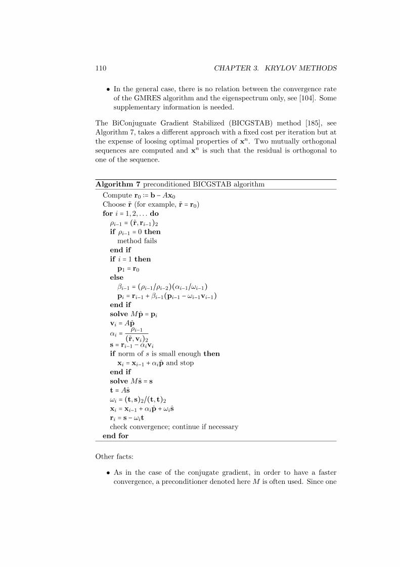
110 CHAPTER 3. KRYLOV METHODS
• In the general case, there is no relation between the convergence rateof the GMRES algorithm and the eigenspectrum only, see [104]. Somesupplementary information is needed.
The BiConjuguate Gradient Stabilized (BICGSTAB) method [185], seeAlgorithm 7, takes a different approach with a fixed cost per iteration but atthe expense of loosing optimal properties of xn. Two mutually orthogonalsequences are computed and xn is such that the residual is orthogonal toone of the sequence.
Algorithm 7 preconditioned BICGSTAB algorithm
Compute r0 ∶= b −Ax0
Choose r (for example, r = r0)for i = 1,2, . . . doρi−1 = (r, ri−1)2
if ρi−1 = 0 thenmethod fails
end ifif i = 1 then
p1 = r0
elseβi−1 = (ρi−1/ρi−2)(αi−1/ωi−1)pi = ri−1 + βi−1(pi−1 − ωi−1vi−1)
end ifsolve M p = pivi = Ap
αi =ρi−1
(r,vi)2s = ri−1 − αiviif norm of s is small enough then
xi = xi−1 + αip and stopend ifsolve M s = st = Asωi = (t, s)2/(t, t)2
xi = xi−1 + αip + ωisri = s − ωitcheck convergence; continue if necessary
end for
Other facts:
• As in the case of the conjugate gradient, in order to have a fasterconvergence, a preconditioner denoted here M is often used. Since one

3.5. KRYLOV METHODS FOR ILL-POSED PROBLEMS 111
doesn’t need to preserve some symmetry, the preconditioned iterationis simply derived from the unpreconditioned one by replacing A byM−1A into Algorithm (6).
• Krylov methods do not need the explicit form of the operators A norof the preconditioner M . They are based on applying these operatorsto vectors (so called matrix vector product operations) as it is the casefor the fixed point method (3.3). These are matrix free methods.
• There exist Matlab functions for the main Krylov methods: pcg forthe Conjugate Gradient and gmres for the GMRES method.
In conclusion fixed point iterations (3.3) generate an approximate solutionxn that belongs to the same Krylov space as CG or GMRES iterate xnKbut with “frozen” coefficients. Thus we have that xn is less (actually muchmuch less) optimal than xnK . In conclusion, As a result, it is convenient toreplace the fixed point method by a Krylov type method.
For more details on these Krylov methods, see [169] for a complete overviewincluding implementation issues, [9] for their templates and for a more math-ematical introduction [103] and for finite precision effects [141].
3.5 Krylov methods for ill-posed problems
Since it will be needed in some sub-structuring methods § 6.5, we considerhere the case where the linear system
Ax = b (3.54)
is square but ill-posed. In order to have existence of a solution, we assumethat b ∈ range(A). A solution is unique up to any element of ker(A). Weshall see that if A is symmetric, Krylov method will converge to a solution.When A is non symmetric, we may not converge to a solution.We start with the symmetric case. It is known in this case that
RN = ker(A)⊕⊥ range(A)
and that there is a unique solution x ∈ range(A) to (3.54) denoted A†b inthe sequel. Thus we have that A† is an isomorphism from range(A) ontoitself.The idea at the origin of Krylov methods can be found in the followinglemma which is true for an invertible matrix.
Lemma 3.5.1 Let C be an invertible matrix of size N × N . Then, thereexists a polynomial P of degree p < N such that
C−1 = P(C) .

112 CHAPTER 3. KRYLOV METHODS
Proof Let
M(X) ∶=d
∑i=0
aiXi
be a minimal polynomial of C of degree d ≤ N . We have that
d
∑i=0
aiCi = 0
and there is no non zero polynomial of lower degree that annihilates C.Thus, a0 cannot be zero. Otherwise, we would have
Cd
∑i=1
aiCi−1 = 0 .
and since C is invertible:d
∑i=1
aiCi−1 = 0 .
Then, ∑d−1i=0 ai+1X
i would be an annihilating polynomial of C of degree lowerthan d. By definition of a minimal polynomial, this is impossible. Thisproves that a0 ≠ 0 and we can divide by a0:
Id +Cd
∑i=1
aia0Ci−1 = 0
that is
C−1 = P(C), P(C) ∶= −d
∑i=1
aia0Ci−1 . (3.55)
Our first step is to extend Lemma 3.5.1 to the non invertible symmetriccase.
Lemma 3.5.2 Let A be a symmetric indefinite matrix of size N ×N . Thenthere exist coefficients (ai)2≤i≤p with p ≤ N such that
A =p
∑i=2
aiAi . (3.56)
Proof Let Λ denote the set of the eigenvalues of A without taking intoaccount their multiplicities. Since matrix A is non invertible, we have 0 ∈ Λ.Moreover, since it is symmetric, it is diagonalizable and it is easy to checkthat A cancels its characteristic polynomial, that is
∏λ∈Λ
(λId −A) = 0 . (3.57)

3.5. KRYLOV METHODS FOR ILL-POSED PROBLEMS 113
The zero-th order term of the above polynomial is zero and the next termis non zero since it takes the following value:
−⎛⎝ ∏λ∈Λ∖0
λ⎞⎠A.
Then, it suffices to expand polynomial from the left-hand side of (3.57),divide it by ∏λ∈Λ∖0 λ and rearrange terms to end the proof.The consequence of this is the following lemma
Lemma 3.5.3 The unique solution to Ay = r that belongs to range(A), fora given r ∈ range(A) can be written as
y =p
∑i=2
aiAi−2 r (3.58)
where the coefficients ai are given in (3.56).
Proof Let r = At ∈ range(A) for some t ∈ RN . Note that since t may havea non zero component in ker(A), we may have y ≠ t. We apply Lemma 3.5.2and right multiply (3.56) by vector t:
A (p
∑i=2
aiAi−2) r
´¹¹¹¹¹¹¹¹¹¹¹¹¹¹¹¹¹¹¹¹¹¹¹¹¹¹¹¹¹¹¹¹¹¹¹¸¹¹¹¹¹¹¹¹¹¹¹¹¹¹¹¹¹¹¹¹¹¹¹¹¹¹¹¹¹¹¹¹¹¹¹¶y∶=
= r .
Thus, we conclude that y given by (3.58) is the unique solution to Ay = rthat belongs to range(A).
We apply now these results to the solving of Ax = b ∈ range(A) by a Krylovmethod with x0 as an initial guess. This result does not depend on theactual implementation of the Krylov method.
Lemma 3.5.4 (Krylov method for undefinite symmetric systems)Let x0 be the initial guess decomposed into its component in kerA andrange(A):
x0 = x0ker + x0
range .
Then, the solution x to equation (3.54) provided by the Krylov method is
x = x0ker +A†b
In other words, the solution to equation (3.54) “selected” by a Kryolv methodis the one whose component in the kernel of A is x0
ker.

114 CHAPTER 3. KRYLOV METHODS
Proof At step n, a Krylov method will seek an approximate solution to
Ay = b −Ax0 ∶= r0 ∈ range(A)in Kn(A, r0). From (3.58), the method will converge in at most p − 1 itera-tions and then the final solution is
x = x0 + y = x0ker + x0
range + y´¹¹¹¹¹¹¹¹¹¹¹¹¹¹¹¹¹¹¸¹¹¹¹¹¹¹¹¹¹¹¹¹¹¹¹¹¹¶
y
with y ∈ range(A). It is then obvious to see that
Ay = A(x0range + y) = Ax0
range + r0 = b.
so that y = A†b.
Thus, we have proved that a Krylov method applied to an indefinite sym-metric linear system makes sense since for n large enough a solution toAx = b ∈ range(A) can be found in x0 +Kn(A, r0).Remark 3.5.1 This is not generally true in the non symmetric case. Forthe general case, we give now a counter-example. Consider the followingsystem:
⎛⎜⎝
0 0 01 0 00 1 0
⎞⎟⎠
x = b =⎛⎜⎝
011
⎞⎟⎠
(3.59)
whose solutions are
x =⎛⎜⎝
110
⎞⎟⎠+R
⎛⎜⎝
001
⎞⎟⎠.
In particular, the first component of any solution is equal to 1. For sakeof simplicity, assume x0 = 0. Then, the first residual r0 = b has its firstcomponent equal to zero. The same holds for Ak r0 for all k ≥ 1. Thus forall n, any vector in the space x0+Kn(A, r0) has its first component equalto zero and cannot be a solution to system (3.59).
3.6 Schwarz preconditioners using FreeFem++
In order to use Schwarz algorithms as a preconditioner in Krylov methods,in addition to the usual ingredients (partition of the mesh, local matricesand restriction operators), we need only the associated matrix-vectorproduct to the global problem as well as the preconditioning method used.
In the following program Aglobal corresponds to the finite element dis-cretization of the variational formulation of the problem to be solved. Wethen need the matrix-vector product of the operator Aglobal with a vectorl.

3.6. SCHWARZ PRECONDITIONERS USING FREEFEM++ 115
func real[int] A(real[int] &x)3
// Matrix vector product with the global matrixVh Ax;Ax[]= Aglobal∗x;
7 return Ax[];
Listing 3.1: ./FreefemCommon/matvecAS.idp
The preconditioning method can be Additive Schwarz (AS) which can befound in the routine
// and the application of the preconditionerfunc real[int] AS(real[int] &l)
13 // Application of the ASM preconditioner// Mˆ−1∗y = \sum RiˆT∗Aiˆ−1∗Ri∗y// Ri restriction operators, Ai =Ri∗A∗RiˆT local matrices
17 Vh s = 0;for(int i=0;i<npart;++i)
real[int] bi = Rih[i]∗l; // restricts rhs
21 real[int] ui = aA[i] −1∗ bi; // local solvess[] += Rih[i]’∗ui; // prolongation
return s[];25
Listing 3.2: ./FreefemCommon/matvecAS.idp

116 CHAPTER 3. KRYLOV METHODS
// Preconditioned Conjugate Gradient Applied to the system3 // A(un[]) = rhsglobal[]
// preconditioned by the linear operator// AS: r[] −> AS(r[])func real[int] myPCG(real[int] xi,real eps, int nitermax)
7 ofstream filei(”Convprec.m”);ofstream fileignu(”Convprec.gnu”);
Vh r, un, p, zr, rn, w, er;11 un[] = xi;
r[] = A(un[]);r[] −= rhsglobal[];r[] ∗= −1.0;
15 zr[] = AS(r[]);real resinit=sqrt(zr[]’∗zr[]);p = zr;for(int it=0;it<nitermax;++it)
19 plot(un,value=1,wait=1,fill=1,dim=3,cmm=”Approximate solution at ⤸
Ç iteration ”+it);real relres = sqrt(zr[]’∗zr[])/resinit;cout << ”It: ”<< it << ” Relative residual = ” << relres << endl;
23 int j = it+1;filei << ”relres(”+j+”)=” << relres << ”;” << endl;fileignu << relres << endl;if(relres < eps)
27 cout << ”CG has converged in ” + it + ” iterations ” << endl;cout << ”The relative residual is ” + relres << endl;break;
31 w[] = A(p[]);real alpha = r[]’∗zr[];real aux2 = alpha;
35 real aux3 = w[]’∗p[];alpha /= aux3; // alpha = (rj,zj)/(Apj,pj);un[] += alpha∗p[]; // xj+1 = xj + alpha∗p;r[] −= alpha∗w[]; // rj+1 = rj − alpha∗Apj;
39 zr[] = AS(r[]); // zj+1 = M−1∗rj+1;real beta = r[]’∗zr[];beta /= aux2; // beta = (rj+1,zj+1)/(rj,zj);p[] ∗= beta;
43 p[] += zr[];
return un[];
Listing 3.3: ./KRYLOV/FreefemProgram/PCG.idp
The Krylov method applied in this case is the Conjugate Gradient (we are inthe symmetric case since both the original problem and the preconditionerare symmetric positive definite) The whole program where these routines

3.6. SCHWARZ PRECONDITIONERS USING FREEFEM++ 117
are called is AS-PCG.edp.
/∗# debutPartition #∗/2 include ”../../FreefemCommon/dataGENEO.edp”
include ”../../FreefemCommon/decomp.idp”include ”../../FreefemCommon/createPartition.idp”SubdomainsPartitionUnity(Th,part[],sizeovr,aTh,Rih,Dih,Ndeg,AreaThi);
6 /∗# endPartition #∗//∗# debutGlobalData #∗/Aglobal = vaglobal(Vh,Vh,solver = UMFPACK); // global matrixrhsglobal[] = vaglobal(0,Vh); // global rhs
10 uglob[] = Aglobal−1∗rhsglobal[];/∗# finGlobalData #∗//∗# debutLocalData #∗/for(int i = 0;i<npart;++i)
14 cout << ” Domain :” << i << ”/” << npart << endl;matrix aT = Aglobal∗Rih[i]’;aA[i] = Rih[i]∗aT;
18 set(aA[i],solver = UMFPACK); // direct solvers using UMFPACK
/∗# finLocalData #∗//∗# debutPCGSolve #∗/
22 include ”../../FreefemCommon/matvecAS.idp”include ”PCG.idp”Vh un = 0, sol; // initial guess un and final solutioncout << ”Schwarz Dirichlet algorithm” << endl;
26 sol[] = myPCG(un[], tol, maxit); // PCG with initial guess unplot(sol,cmm=” Final solution”, wait=1,dim=3,fill=1,value=1);Vh er = sol−uglob;cout << ” Final error: ” << er[].linfty << endl;
30 /∗# finPCGSolve #∗/
Listing 3.4: ./KRYLOV/FreefemProgram/AS-PCG.edp
In the three-dimensional case the only thing that changes with respect tothe main script is the preparation of the data
include ”../../FreefemCommon/data3d.edp”3 include ”../../FreefemCommon/decomp3d.idp”
include ”../../FreefemCommon/createPartition3d.idp”SubdomainsPartitionUnity3(Th,part[],sizeovr,aTh,Rih,Dih,Ndeg,VolumeThi);
Listing 3.5: ./KRYLOV/FreefemProgram/AS-PCG3d.edp
We can also use RAS as a preconditioner in GMRES or BiCGSTAB,by slightly modifying the program as described in the following rou-tines:
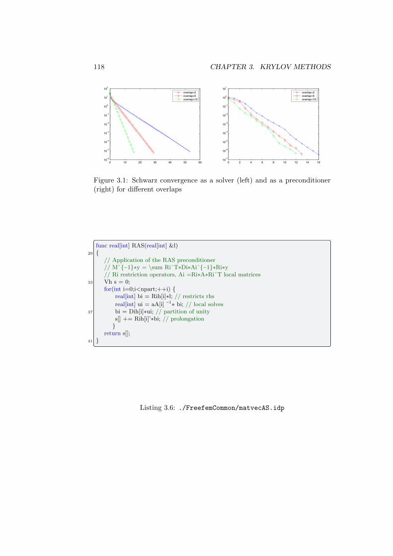
118 CHAPTER 3. KRYLOV METHODS
0 10 20 30 40 50 6010 6
10 5
10 4
10 3
10 2
10 1
100
101
102
overlap=2overlap=5overlap=10
0 2 4 6 8 10 12 14 1610 7
10 6
10 5
10 4
10 3
10 2
10 1
100
101
overlap=2overlap=5overlap=10
Figure 3.1: Schwarz convergence as a solver (left) and as a preconditioner(right) for different overlaps
func real[int] RAS(real[int] &l)29
// Application of the RAS preconditioner// Mˆ−1∗y = \sum RiˆT∗Di∗Aiˆ−1∗Ri∗y// Ri restriction operators, Ai =Ri∗A∗RiˆT local matrices
33 Vh s = 0;for(int i=0;i<npart;++i)
real[int] bi = Rih[i]∗l; // restricts rhs
real[int] ui = aA[i] −1∗ bi; // local solves37 bi = Dih[i]∗ui; // partition of unity
s[] += Rih[i]’∗bi; // prolongation
return s[];41
Listing 3.6: ./FreefemCommon/matvecAS.idp
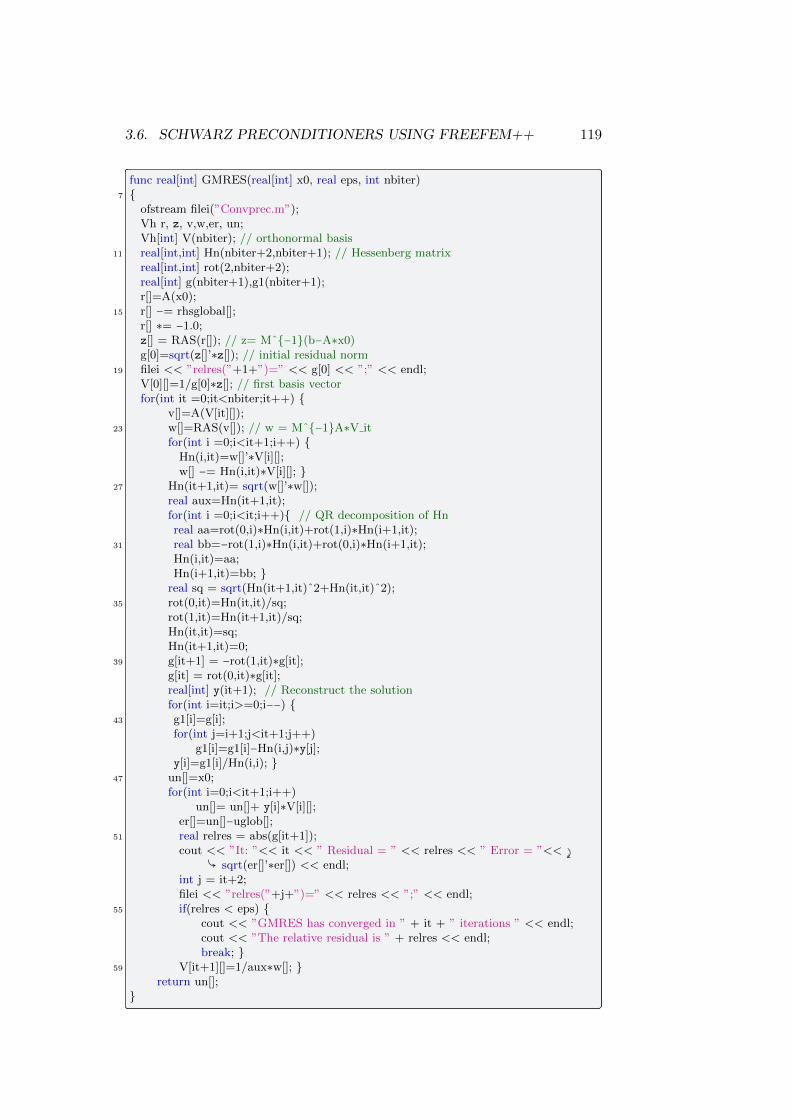
3.6. SCHWARZ PRECONDITIONERS USING FREEFEM++ 119
func real[int] GMRES(real[int] x0, real eps, int nbiter)7
ofstream filei(”Convprec.m”);Vh r, z, v,w,er, un;Vh[int] V(nbiter); // orthonormal basis
11 real[int,int] Hn(nbiter+2,nbiter+1); // Hessenberg matrixreal[int,int] rot(2,nbiter+2);real[int] g(nbiter+1),g1(nbiter+1);r[]=A(x0);
15 r[] −= rhsglobal[];r[] ∗= −1.0;z[] = RAS(r[]); // z= Mˆ−1(b−A∗x0)g[0]=sqrt(z[]’∗z[]); // initial residual norm
19 filei << ”relres(”+1+”)=” << g[0] << ”;” << endl;V[0][]=1/g[0]∗z[]; // first basis vectorfor(int it =0;it<nbiter;it++)
v[]=A(V[it][]);23 w[]=RAS(v[]); // w = Mˆ−1A∗V it
for(int i =0;i<it+1;i++) Hn(i,it)=w[]’∗V[i][];w[] −= Hn(i,it)∗V[i][];
27 Hn(it+1,it)= sqrt(w[]’∗w[]);real aux=Hn(it+1,it);for(int i =0;i<it;i++) // QR decomposition of Hnreal aa=rot(0,i)∗Hn(i,it)+rot(1,i)∗Hn(i+1,it);
31 real bb=−rot(1,i)∗Hn(i,it)+rot(0,i)∗Hn(i+1,it);Hn(i,it)=aa;Hn(i+1,it)=bb;
real sq = sqrt(Hn(it+1,it)ˆ2+Hn(it,it)ˆ2);35 rot(0,it)=Hn(it,it)/sq;
rot(1,it)=Hn(it+1,it)/sq;Hn(it,it)=sq;Hn(it+1,it)=0;
39 g[it+1] = −rot(1,it)∗g[it];g[it] = rot(0,it)∗g[it];real[int] y(it+1); // Reconstruct the solutionfor(int i=it;i>=0;i−−)
43 g1[i]=g[i];for(int j=i+1;j<it+1;j++)
g1[i]=g1[i]−Hn(i,j)∗y[j];y[i]=g1[i]/Hn(i,i);
47 un[]=x0;for(int i=0;i<it+1;i++)
un[]= un[]+ y[i]∗V[i][];er[]=un[]−uglob[];
51 real relres = abs(g[it+1]);cout << ”It: ”<< it << ” Residual = ” << relres << ” Error = ”<< ⤸
Ç sqrt(er[]’∗er[]) << endl;int j = it+2;filei << ”relres(”+j+”)=” << relres << ”;” << endl;
55 if(relres < eps) cout << ”GMRES has converged in ” + it + ” iterations ” << endl;cout << ”The relative residual is ” + relres << endl;break;
59 V[it+1][]=1/aux∗w[]; return un[];

120 CHAPTER 3. KRYLOV METHODS
Listing 3.7: ./KRYLOV/FreefemProgram/GMRES.idp

3.6. SCHWARZ PRECONDITIONERS USING FREEFEM++ 121
func real[int] BiCGstab(real[int] xi, real eps, int nbiter)7 ofstream filei(”Convprec.m”);
Vh r, rb, rs, er, un, p, yn, zn, z, v, t, tn;un[]=xi;r[]=A(un[]);
11 r[] −= rhsglobal[];r[] ∗= −1.0;rb[]=r[];real rho=1.;
15 real alpha=1.;real omega=1.;z[] = RAS(r[]);real resinit=sqrt(z[]’∗z[]);
19 p[]=0; v[]=0;real rhonew, beta;for(int it =1;it<nbiter;it++)
real relres = sqrt(z[]’∗z[])/resinit;23 cout << ”It: ”<< it << ” Relative residual = ” << relres << endl;
int j = it+1;filei << ”relres(”+j+”)=” << relres << ”;” << endl;if(relres < eps)
27 cout << ”BiCGstab has converged in ” + it + ” iterations ” << endl;cout << ”The relative residual is ” + relres << endl;break;
31 rhonew=rb[]’∗r[]; // rhoi = (rb,rim1);beta=(rhonew/rho)∗(alpha/omega); // beta = (rhoi/rhoim1)∗(alpha/omega);p[] −=omega∗v[]; // pi = rim1 + beta∗(pim1 − omega∗vim1);p[] ∗= beta;
35 p[] += r[];yn[] = RAS(p[]); // y = Mm1∗pi; vi = A∗y;v[] = A(yn[]);alpha = rhonew/(rb[]’∗v[]); // alpha = rhoi/(rb’∗vi);
39 rs[] = r[]; // s = rim1 − alpha∗vi;rs[] −= alpha∗v[];zn[] = RAS(rs[]); // z = Mm1∗s; t = A∗z;t[] = A(zn[]);
43 tn[] = RAS(t[]); // tn = Mm1∗t;omega = (tn[]’∗zn[])/(tn[]’∗tn[]); // omega = ⤸
Ç (Mm1∗t,Mm1∗s)/(Mm1∗t,Mm1∗t);un[] += alpha∗yn[]; // xi = xim1 + alpha∗y + omega∗z;un[] += omega∗zn[];
47 r[] = rs[];r[] −= omega∗t[];z[] = RAS(r[]);rho = rhonew;
51 return un[];
Listing 3.8: ./KRYLOV/FreefemProgram/BiCGstab.idp
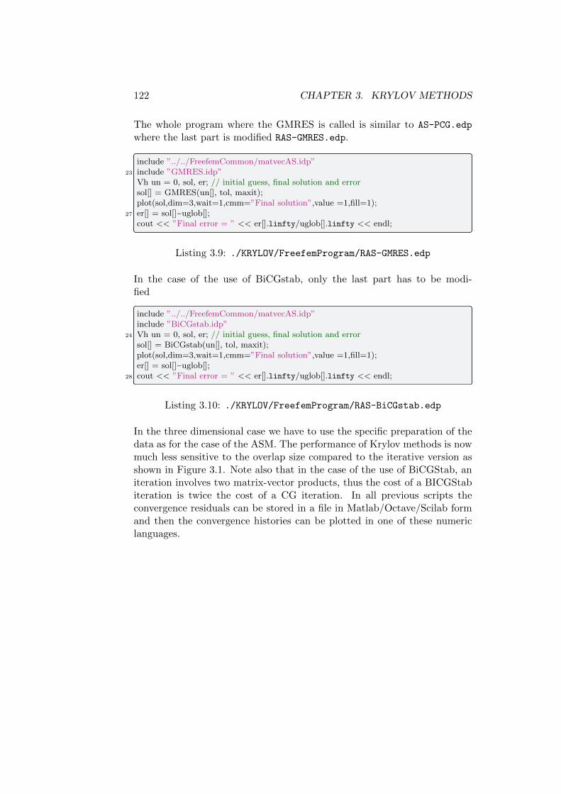
122 CHAPTER 3. KRYLOV METHODS
The whole program where the GMRES is called is similar to AS-PCG.edp
where the last part is modified RAS-GMRES.edp.
include ”../../FreefemCommon/matvecAS.idp”23 include ”GMRES.idp”
Vh un = 0, sol, er; // initial guess, final solution and errorsol[] = GMRES(un[], tol, maxit);plot(sol,dim=3,wait=1,cmm=”Final solution”,value =1,fill=1);
27 er[] = sol[]−uglob[];cout << ”Final error = ” << er[].linfty/uglob[].linfty << endl;
Listing 3.9: ./KRYLOV/FreefemProgram/RAS-GMRES.edp
In the case of the use of BiCGstab, only the last part has to be modi-fied
include ”../../FreefemCommon/matvecAS.idp”include ”BiCGstab.idp”
24 Vh un = 0, sol, er; // initial guess, final solution and errorsol[] = BiCGstab(un[], tol, maxit);plot(sol,dim=3,wait=1,cmm=”Final solution”,value =1,fill=1);er[] = sol[]−uglob[];
28 cout << ”Final error = ” << er[].linfty/uglob[].linfty << endl;
Listing 3.10: ./KRYLOV/FreefemProgram/RAS-BiCGstab.edp
In the three dimensional case we have to use the specific preparation of thedata as for the case of the ASM. The performance of Krylov methods is nowmuch less sensitive to the overlap size compared to the iterative version asshown in Figure 3.1. Note also that in the case of the use of BiCGStab, aniteration involves two matrix-vector products, thus the cost of a BICGStabiteration is twice the cost of a CG iteration. In all previous scripts theconvergence residuals can be stored in a file in Matlab/Octave/Scilab formand then the convergence histories can be plotted in one of these numericlanguages.

Chapter 4
Coarse Spaces
Theoretical and numerical results show that domain decomposition methodsbased solely on local subdomain solves are not scalable with respect to thenumber of subdomains. This can be fixed by using a two-level method inwhich the preconditioner is enriched by the solve of a coarse problem whosesize is of the order of the number of subdomains. In § 4.1, we see that onelevel Schwarz methods are not scalable since the iteration count grows asthe number of subdomains in one direction. We present a fix introduced inNicolaides [151]. A numerical implementation is given in § 4.2.1. In § 5.1
4.1 Need for a two-level method
The results presented so far concern only a small number of subdomains,two for the theoretical results of § 1.5 and four for the numerical resultsof § 3.6. When the number of subdomains is large, plateaus appear in theconvergence of Schwarz domain decomposition methods. This is the caseeven for a simple model such as the Poisson problem:
−∆u = f, in Ω,u = 0, on ∂Ω.
The problem of one level method comes from the fact that in the Schwarzmethods of § 1 there is a lack of a global exchange of information. Data are
Figure 4.1: Decomposition into many subdomains
123

124 CHAPTER 4. COARSE SPACES
exchanged only from one subdomain to its direct neighbors. But the solutionin each subdomain depends on the right-hand side in all subdomains. Letus denote by Nd the number of subdomains in one direction. Then, forinstance, the leftmost domain of Figure 4.1 needs at least Nd iterationsbefore being aware about the value of the right-hand side f in the rightmostsubdomain. The length of the plateau is thus typically related to the numberof subdomains in one direction and therefore to the notion of scalability metin the context of high performance computing.To be more precise, there are two common notions of scalability.
Definition 4.1.1 (Strong scalability) Strong scalability is defined ashow the solution time varies with the number of cores for a fixed total prob-lem size. Ideally, the elapsed time is inversely proportional to the number ofcores.
Definition 4.1.2 (Weak scalability) Weak scalability is defined as howthe solution time varies with the number of cores for a fixed problem size percore. Ideally the elapsed time is constant for a fixed ratio between the sizeof the problem and the number of cores.
A mechanism through which the scalability can be achieved (in this case theweak scalability) consists in the introduction of a two-level preconditionervia a coarse space correction. In two-level methods, a small problem ofsize typically the number of subdomains couples all subdomains at eachiteration. Note that here the term scalable refers to the number of iterations.In real applications, scalability is defined in terms of the total computingtime. When measured by the computing time, the two-level methods areoften not scalable for large scale calculation because the coarse grid solveris not scalable. As a result, a multilevel (more than two) approach is oftennecessary.To illustrate the need of a coarse space, in Figure 4.2 we consider a 2Dproblem decomposed into 2×2, 4×4 and 8×8 subdomains. For each domaindecomposition, we have two curves: one with a one-level method which haslonger and longer plateaus and the second curve with a coarse grid correctionwhich is denoted by M2 for which plateaus are much smaller. The problemof one level methods and its cure are also well illustrated in Figure 4.3 fora domain decomposition into 64 strips as well as in Table 4.1. The onelevel method has a long plateau in the convergence whereas with a coarsespace correction convergence is quite fast. We also see that for the one-levelcurves, the plateau has a size proportional to the number of subdomains inone direction. This can be understood by looking at Figure 4.4 where weplot the slow decrease of the error for a one dimensional Poisson problem.From the linear algebra point of view, stagnation in the convergence of one-level Schwarz methods corresponds to a few very low eigenvalues in thespectrum of the preconditioned problem. Using preconditioners M−1
ASM or

4.1. NEED FOR A TWO-LEVEL METHOD 125
-7
-6
-5
-4
-3
-2
-1
0
0 10 20 30 40 50 60 70 80
Log_10 (
Err
or)
Number of iterations (GCR)
M22x2
2x2 M24x4
M28x8
4x4 8x8
Figure 4.2: Japhet, Nataf, Roux (1998)
M−1RAS , we can remove the influence of very large eigenvalues of the coeffi-
cient matrix, which correspond to high frequency modes. It has been provedthat for a SPD (symmetric positive definite) matrix, the largest eigenvalueof the preconditioned system by M−1
ASM is bounded by the number of col-ors needed for the overlapping decomposition such that different colors areused for adjacent subdomains, see [184] or [169] for instance. But the smalleigenvalues still exist and hamper the convergence. These small eigenvaluescorrespond to low frequency modes and represent a certain global informa-tion with which we have to deal efficiently.A classical remedy consists in the introduction of a coarse grid or coarsespace correction that couples all subdomains at each iteration of the iterativemethod. This is closely related to deflation technique classical in linearalgebra, see Nabben and Vuik’s paper [183] and references therein. This isconnected as well to augmented or recycled Krylov space methods, see e.g.[76], [154] [168] or [23] and references therein.Suppose we have identified the modes corresponding to the slow convergenceof the iterative method used to solve the linear system:
Ax = b
with a preconditioner M , in our case a domain decomposition method. Thatis, we have some a priori knowledge on the small eigenvalues of the precondi-tioned system M−1A. For a Poisson problem, these slow modes correspondto constant functions that are in the null space (kernel) of the Laplace op-erators. For a homogeneous elasticity problem, they correspond to the rigidbody motions.Let us call Z the rectangular matrix whose columns correspond to theseslow modes. There are algebraic ways to incorporate this information to

126 CHAPTER 4. COARSE SPACES
accelerate the method. We give here the presentation that is classical indomain decomposition, see e.g. [137] or [184]. In the case where A is SPD,the starting point is to consider the minimization problem
minβ
∥A(y +Zβ) − b∥A−1 .
It corresponds to finding the best correction to an approximate solution yby a vector Zβ in the vector space spanned by the nc columns of Z. Thisproblem is equivalent to
minβ∈Rnc
2(Ay − b, Zβ)2 + (AZβ,Zβ)2
and whose solution is:
β = (ZTAZ)−1ZT (b −Ay) .
Thus, the correction term is:
Zβ = Z (ZTAZ)−1ZT (b −Ay)´¹¹¹¹¹¹¹¹¹¹¹¹¹¹¹¹¸¹¹¹¹¹¹¹¹¹¹¹¹¹¹¹¹¶
r
.
This kind of correction is called a Galerkin correction. Let R0 ∶= ZT andr = b−Ay be the residual associated to the approximate solution y. We havejust seen that the best correction that belongs to the vector space spannedby the columns of Z reads:
Zβ = RT0 β = RT0 (R0ART0 )−1R0r .
When using such an approach with an additive Schwarz method (ASM) asdefined in eq. (1.29), it is natural to introduce an additive correction to theadditive Schwarz method.
Definition 4.1.3 (Two-level additive Schwarz preconditioner) Thetwo-level additive Schwarz preconditioner is defined as
M−1ASM,2 ∶= RT0 (R0AR
T0 )−1
R0 +N
∑i=1
RTi (RiARTi )−1Ri (4.1)
where the Ri’s (1 ≤ i ≤ N) are the restriction operators to the overlappingsubdomains and R0 = ZT .
Remark 4.1.1 This definition suggests the following remarks.
• The structure of the two level preconditioner M−1ASM,2 is the same that
of the one level method.

4.1. NEED FOR A TWO-LEVEL METHOD 127
N subdomains Schwarz With coarse grid
4 18 25
8 37 22
16 54 24
32 84 25
64 144 25
Table 4.1: Iteration counts for a Poisson problem on a domain decomposedinto strips. The number of unknowns is proportional to the number ofsubdomains (weak scalability).
• Compared to the one level Schwarz method where only local subprob-lems have to be solved in parallel, the two-level method adds the solvingof a linear system of matrix R0AR
T0 which is global in nature. This
global problem is called coarse problem.
• The coarse problem couples all subdomains at each iteration but itsmatrix is a small O(N ×N) square matrix and the extra cost is neg-ligible compared to the gain provided the number of subdomains is nottoo large.
In Table 4.1 we display the iteration counts for a decomposition of thedomain in an increasing number of subdomains. In figure 4.3, we see thatwithout a coarse grid correction, the convergence curve of the one levelSchwarz method has a very long plateau that can be bypassed by a two-level method.
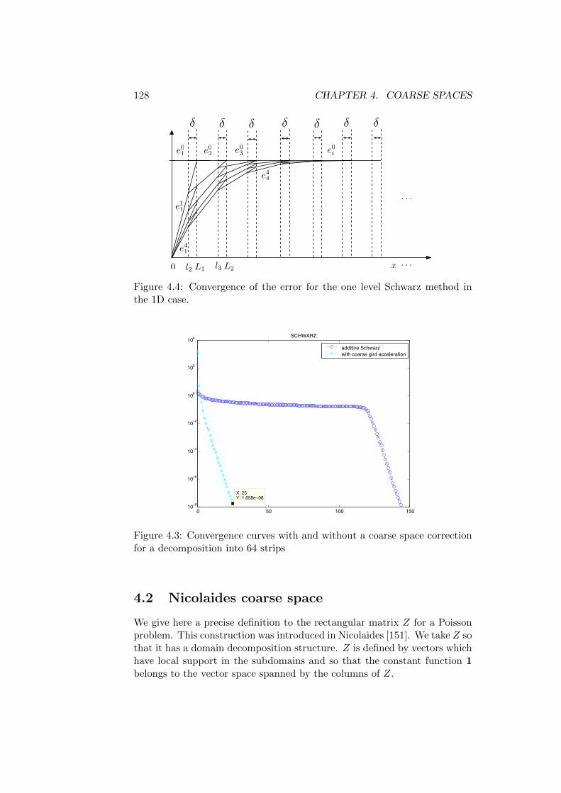
128 CHAPTER 4. COARSE SPACES
L1l20 x
l3 L2
. . .
. . .
e11
e41
e44
e01 e0
2 e03 e0
i
Figure 4.4: Convergence of the error for the one level Schwarz method inthe 1D case.
0 50 100 15010−8
10−6
10−4
10−2
100
102
104
X: 25Y: 1.658e−08
SCHWARZ
additive Schwarzwith coarse gird acceleration
Figure 4.3: Convergence curves with and without a coarse space correctionfor a decomposition into 64 strips
4.2 Nicolaides coarse space
We give here a precise definition to the rectangular matrix Z for a Poissonproblem. This construction was introduced in Nicolaides [151]. We take Z sothat it has a domain decomposition structure. Z is defined by vectors whichhave local support in the subdomains and so that the constant function 1belongs to the vector space spanned by the columns of Z.

4.2. NICOLAIDES COARSE SPACE 129
Recall first that we have a discrete partition of unity (see § 1.3) in thefollowing sense: let Ni be subsets of indices, Di be diagonal matrices, 1 ≤i ≤ N :
Di ∶ R#Ni z→ R#Ni (4.2)
so that we have:N
∑i=1
RTi DiRi = Id .
With these ingredients we are ready to provide the definition of what wewill further call classical or Nicolaides coarse space.
Definition 4.2.1 (Nicolaides coarse space) We define Z as the matrixwhose i-th column is
Zi ∶= RTi DiRi1 for 1 ≤ i ≤ N (4.3)
where 1 is the vector of dimension N full of ones. The global structure ofZ is thus the following:
Z =
⎡⎢⎢⎢⎢⎢⎢⎢⎣
D1R11 0 ⋯ 00 D2R21 ⋱⋮ ⋱ ⋱ 00 0 0 DNRN1
⎤⎥⎥⎥⎥⎥⎥⎥⎦
. (4.4)
Numerical results of Figures 4.3 and Table 4.1 have been obtained by a two-level Schwarz preconditioner (4.1) where R0 = ZT with Z being defined by(4.4).
4.2.1 Nicolaides coarse space using FreeFem++
We provide FreeFem++ scripts that will illustrate numerically the perfor-mance of the Nicolaides coarse space. We need first to build matrix Z whoseexpression is given in (4.4),
// Build coarse spacefor(int i=0;i<npart;++i)
4 Z[i]=1.;// Z[i][] = Z[i][].∗intern[];real[int] zit = Rih[i]∗Z[i][];
8 real[int] zitemp = Dih[i]∗zit;Z[i][]=Rih[i]’∗zitemp;
Listing 4.1: ./FreefemCommon/coarsespace.idp
then the coarse matrix A0 = ZTAZ = R0ART0 ,

130 CHAPTER 4. COARSE SPACES
13 real[int,int] Ef(npart,npart); // E = ZˆT∗A∗Zfor(int i=0;i<npart;++i)
real[int] vaux = A(Z[i][]);17 for(int j=0;j<npart;++j)
Ef(j,i) = Z[j][]’∗vaux;
21 matrix E;E = Ef;set(E,solver=UMFPACK);
Listing 4.2: ./FreefemCommon/coarsespace.idp
the coarse solver Q = RT0 (R0ART0 )−1R0
func real[int] Q(real[int] &l) // Q = Z∗E−1∗ZˆT
29 real[int] res(l.n);res=0.;real[int] vaux(npart);for(int i=0;i<npart;++i)
33 vaux[i]=Z[i][]’∗l;
real[int] zaux=E−1∗vaux; // zaux=E−1∗ZˆT∗l
37 for(int i=0;i<npart;++i) // Z∗zaux
res +=zaux[i]∗Z[i][];
41 return res;
Listing 4.3: ./FreefemCommon/coarsespace.idp
the projector outside the coarse space P = I −QA and its transpose P T =I −AQ.

4.2. NICOLAIDES COARSE SPACE 131
45 func real[int] P(real[int] &l) // P = I − A∗Q
real[int] res=Q(l);real[int] res2=A(res);
49 res2 −= l;res2 ∗= −1.;return res2;
53 func real[int] PT(real[int] &l) // PˆT = I−Q∗A
real[int] res=A(l);real[int] res2=Q(res);
57 res2 −= l;res2 ∗= −1.;return res2;
Listing 4.4: ./FreefemCommon/coarsespace.idp
Based on the previous quantities, we can build two versions of the additiveSchwarz preconditioner. First the classical one, called AS2 corresponding tothe formula (4.1) and then, the alternative hybrid version Q + P TM−1
AS,1Pdetailed in § 7.5.
func real[int] AS2(real[int] & r)real[int] z = Q(r);
8 real[int] aux = AS(r);z += aux;return z;
12 func real[int] BNN(real[int] &u) // precond BNN
real[int] aux1 = Q(u);real[int] aux2 = P(u);
16 real[int] aux3 = AS(aux2);aux2 = PT(aux3);aux2 += aux1;
return aux2;20
Listing 4.5: ./COARSEGRID/FreefemProgram/PCG-CS.idp
After that we can use one of these inside a preconditioned conjugate gradient.Finally the main program script is given by AS2-PCG.edp, whose first partis identical as in the case of the one-level method.

132 CHAPTER 4. COARSE SPACES
Figure 4.5: Decomposition into subdomains
include ”../../FreefemCommon/matvecAS.idp”include ”../../FreefemCommon/coarsespace.idp”
24 include ”PCG−CS.idp”Vh un = 0, sol; // initial guess un and final solutioncout << ”Schwarz Dirichlet algorithm” << endl;sol[] = myPCG(un[], tol, maxit); // PCG with initial guess un
28 plot(sol,cmm=” Final solution”, wait=1,dim=3,fill=1,value=1);Vh er = sol−uglob;cout << ” Final error: ” << er[].linfty << endl;
Listing 4.6: ./COARSEGRID/FreefemProgram/AS2-PCG.edp
An identical thing can be performed for the non-symmetric preconditioner,by simply replacing AS by RAS in the two versions of the preconditoners.After that we can use one of these inside a BiCGstab or a GMRES.
6 func real[int] RAS2(real[int] & r)real[int] z = Q(r);real[int] aux = RAS(r);z += aux;
10 return z;func real[int] BNN(real[int] &u) // precond BNN
14 real[int] aux1 = Q(u);real[int] aux2 = P(u);real[int] aux3 = RAS(aux2);aux2 = PT(aux3);
18 aux2 += aux1;return aux2;
Listing 4.7: ./COARSEGRID/FreefemProgram/BiCGstab-CS.idp
We perform now the following numerical experiment: consider a uniformdecomposition into n×n square subdomains where each domain has 20× 20discretization points with two layers of overlap. We see that in the absenceof the coarse space, the iteration number of a Schwarz method used asa preconditioner in a Krylov method, depends linearly on the number of

4.2. NICOLAIDES COARSE SPACE 133
0 10 20 30 40 50 60 7010−8
10−7
10−6
10−5
10−4
10−3
10−2
10−1
100
Iteration
Res
idua
l nor
m (l
ogsc
ale)
2x2 subdomains4x4 subdomains8x8 subdomains
0 5 10 15 20 2510−8
10−7
10−6
10−5
10−4
10−3
10−2
10−1
100
Iteration
Res
idua
l nor
m (l
ogsc
ale)
2x2 subdomains4x4 subdomains8x8 subdomains
Figure 4.6: Convergence history without and with coarse space for variousdomain decompositions
subdomains in one direction. By introducing the Nicolaides coarse space weremove this dependence on the number of subdomains.

134 CHAPTER 4. COARSE SPACES

Chapter 5
Theory of two-level AdditiveSchwarz methods
In this chapter we first introduce first the spectral coarse space which gen-eralizes the idea of Nicolaides coarse space. In order to quantify the actionof this new preconditioner we need to estimate the condition number of thepreconditioned matrix M−1
ASM,2A. This requires a theoretical framework al-lowing a functional analysis of the condition number of the two-level Schwarzmethod with this spectral coarse space.
5.1 Introduction of a spectral coarse space
In this section we introduce a more general coarse space construction thatreduces to that of Nicolaides for a particular choice of a threshold parameter.This new construction answers to the natural question on how to enrichthe coarse space by allowing it to have a size larger than the number ofsubdomains. This enrichment is mainly motivated by the complexity of theproblem to solve, which is often a result of highly heterogeneous coefficients.We will try to keep it for the moment as elementary as possible without anytheoretical convergence proof in this chapter.Classical coarse spaces are known to give good results when the jumps in
Ω1 Ω2
Figure 5.1: Coefficient α varying along and across the interface.
135
136 CHAPTER 5. THEORY OF TWO-LEVEL ASM
the coefficients are across subdomain interfaces (see e.g. [64, 133, 49, 50])or inside the subdomains and not near their boundaries (cf. [160, 159]).However, when the discontinuities are along subdomain interfaces, classicalmethods do not work anymore. In [147], we proposed the constructionof a coarse subspace for a scalar elliptic positive definite operator, whichleads to a two-level method that is observed to be robust with respectto heterogeneous coefficients for fairly arbitrary domain decompositions,e.g. provided by an automatic graph partitioner such as METIS or SCOTCH[120, 26]. This method was extensively studied from the numerical pointof view in [148]. The main idea behind the construction of the coarsespace is the computation of the low-frequency modes associated witha generalized eigenvalue problem based on the Dirichlet-to-Neumann(DtN) map on the boundary of each subdomain. We use the harmonicextensions of these low-frequency modes to the whole subdomain tobuild the coarse space. With this method, even for discontinuities along(rather than across) the subdomain interfaces (cf. Fig. 5.1), the iterationcounts are robust to arbitrarily large jumps of the coefficients leadingto a very efficient, automatic preconditioning method for scalar hetero-geneous problems. As usual with domain decomposition methods, it isalso well suited for parallel implementation as it has been illustrated in [118].
We first motivate why the use of spectral information local to the sub-domains is the key ingredient in obtaining an optimal convergence. Afull mathematical analysis of the two-level method will be given in chapter 5.
We now propose a construction of the coarse space that will be suitable forparallel implementation and efficient for arbitrary domain decompositionsand highly heterogeneous problems such as the Darcy problem with Dirichletboundary conditions:
−div(α∇u) = f, in Ω
where α can vary of several orders of magnitude, typically between 1 and 106.
We still choose Z such that it has the form
Z =
⎡⎢⎢⎢⎢⎢⎢⎢⎣
W 1 0 ⋯ 0⋮ W 2 ⋯ 0⋮ ⋮ ⋯ ⋮0 0 ⋯ WN
⎤⎥⎥⎥⎥⎥⎥⎥⎦
, (5.1)
where N is the number of overlapping subdomains. But W i is now arectangular matrix whose columns are based on the harmonic extensionsof the eigenvectors corresponding to small eigenvalues of the DtN map ineach subdomain Ωi multiplied by the local component of the partition ofunity, see definition 5.5.1. Note that the sparsity of the coarse operator
5.1. INTRODUCTION OF A SPECTRAL COARSE SPACE 137
E = ZTAZ is a result of the sparsity of Z. The nonzero components of Ecorrespond to adjacent subdomains.
More precisely, let us consider first at the continuous level the Dirichlet toNeumann map DtNΩi .
Definition 5.1.1 (Dirichlet-to-Neumann map) For any function de-fined on the interface uΓi ∶ Γi ↦ R, we consider the Dirichlet-to-Neumannmap
DtNΩi(uΓi) =∂v
∂ni∣Γi
,
where Γi ∶= ∂Ωi ∖ ∂Ω and v satisfies
⎧⎪⎪⎪⎨⎪⎪⎪⎩
−div(α∇v) = 0, in Ωi,v = uΓi , on Γi,v = 0, on ∂Ωi ∩ ∂Ω.
(5.2)
If the subdomain is not a floating one (i.e. ∂Ωi ∩ ∂Ω ≠ ∅), we use on∂Ωi ∩ ∂Ω the boundary condition from the original problem v = 0.
To construct the coarse grid subspace, we use some low frequency modes ofthe DtN operator by solving the following eigenvalue problem
DtNΩi(u) = λu. (5.3)
In order to obtain the variational formulation of (5.3) we multiply (5.2) bya test function w, equal to zero on ∂Ωi ∩ ∂Ω
∫Ωiα∇v ⋅ ∇w − ∫
Γiα∂v
∂niw = 0.
By using the fact that
α∂v
∂ni= λαv on Γi and w = 0 on ∂Ωi ∩ ∂Ω
we get the variational formulation of the eigenvalue problem of the localDirichlet-to-Neumann map
Find (v, λ) such that ∫Ωiα∇v ⋅ ∇w = λ∫
∂Ωiαvw, ∀w. (5.4)
We now motivate our choice of this coarse space based on DtN map. Wewrite the original Schwarz method at the continuous level, where the domainΩ is decomposed in a one-way partitioning. The error eni between the currentiterate at step n of the algorithm and the solution u∣Ωi (eni ∶= uni − u∣Ωi) insubdomain Ωi at step n of the algorithm is harmonic
− div(α∇en+1i ) = 0 in Ωi . (5.5)
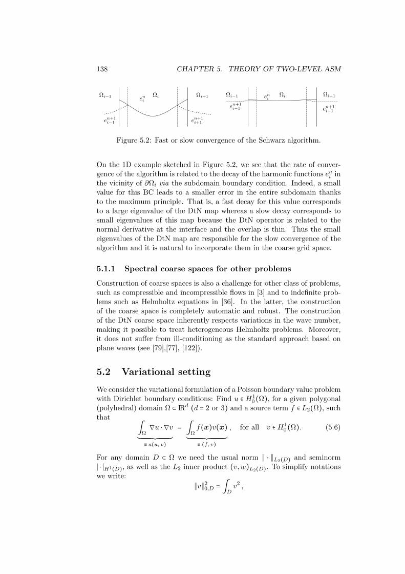
138 CHAPTER 5. THEORY OF TWO-LEVEL ASM
Ωi Ωi+1Ωi−1 eni
en+1i−1 en+1
i+1
Ωi Ωi+1Ωi−1 eni
en+1i−1 en+1
i+1
Figure 5.2: Fast or slow convergence of the Schwarz algorithm.
On the 1D example sketched in Figure 5.2, we see that the rate of conver-gence of the algorithm is related to the decay of the harmonic functions eni inthe vicinity of ∂Ωi via the subdomain boundary condition. Indeed, a smallvalue for this BC leads to a smaller error in the entire subdomain thanksto the maximum principle. That is, a fast decay for this value correspondsto a large eigenvalue of the DtN map whereas a slow decay corresponds tosmall eigenvalues of this map because the DtN operator is related to thenormal derivative at the interface and the overlap is thin. Thus the smalleigenvalues of the DtN map are responsible for the slow convergence of thealgorithm and it is natural to incorporate them in the coarse grid space.
5.1.1 Spectral coarse spaces for other problems
Construction of coarse spaces is also a challenge for other class of problems,such as compressible and incompressible flows in [3] and to indefinite prob-lems such as Helmholtz equations in [36]. In the latter, the constructionof the coarse space is completely automatic and robust. The constructionof the DtN coarse space inherently respects variations in the wave number,making it possible to treat heterogeneous Helmholtz problems. Moreover,it does not suffer from ill-conditioning as the standard approach based onplane waves (see [79],[77], [122]).
5.2 Variational setting
We consider the variational formulation of a Poisson boundary value problemwith Dirichlet boundary conditions: Find u ∈ H1
0(Ω), for a given polygonal(polyhedral) domain Ω ⊂ IRd (d = 2 or 3) and a source term f ∈ L2(Ω), suchthat
∫Ω∇u ⋅ ∇v
´¹¹¹¹¹¹¹¹¹¹¹¹¹¹¹¹¹¹¹¹¹¹¹¹¸¹¹¹¹¹¹¹¹¹¹¹¹¹¹¹¹¹¹¹¹¹¹¹¹¹¶≡ a(u, v)
= ∫Ωf(x)v(x)
´¹¹¹¹¹¹¹¹¹¹¹¹¹¹¹¹¹¹¹¹¹¹¹¹¹¹¹¹¹¹¹¸¹¹¹¹¹¹¹¹¹¹¹¹¹¹¹¹¹¹¹¹¹¹¹¹¹¹¹¹¹¹¹¹¶≡ (f, v)
, for all v ∈H10(Ω). (5.6)
For any domain D ⊂ Ω we need the usual norm ∥ ⋅ ∥L2(D) and seminorm∣ ⋅ ∣H1(D), as well as the L2 inner product (v,w)L2(D). To simplify notationswe write:
∥v∥20,D = ∫
Dv2 ,

5.3. ADDITIVE SCHWARZ SETTING 139
and the seminorm ∣ ⋅ ∣a,D is defined by
∣v∣2a,D = ∫D
∣∇v∣2 .
When D = Ω we omit the domain from the subscript and write ∥ ⋅ ∥0 and∣ ⋅ ∣a instead of ∥ ⋅ ∥0,Ω and ∣ ⋅ ∣a,Ω respectively. Note that the seminorm ∣ ⋅ ∣abecomes a norm on H1
0(Ω).Finally, we will also need averages and norms defined on (d−1)–dimensionalmanifolds X ⊂ IRd, namely for any v ∈ L2(X) we define
vX ∶= 1
∣X ∣ ∫X u and ∥v∥20,X ∶= ∫
Xv2.
where ∣X ∣ is the measure of the manifold X.We consider a discretization of the variational problem (5.6) with P1 con-tinuous, piecewise linear finite elements (FE). To define the FE spaces andthe approximate solution, we assume that we have a shape regular, sim-plicial triangulation Th of Ω. The standard space of continuous and piece-wise linear (w.r.t Th) functions is then denoted by Vh, and the subspace offunctions from Vh that vanish on the boundary of Ω by Vh,0. Note thatVh,0 = Vh ∩H1
0(Ω). Denote by φkk∈N the basis of Vh,0 and xkk∈N theassociated nodes in Ω. Let us write the discrete FE problem that we wantto solve: Find uh ∈ Vh,0 such that
a(uh, vh) = (f, vh), for all vh ∈ Vh,0. (5.7)
which gives the matrix form
AU = F, Aij = a(φj , φi), Fi = (f, φi), ∀i, j ∈ N .
so that uh = ∑k∈N Uk φk where U = (Uk)k∈N .For technical reasons, we also need the standard nodal value interpolationoperator Ih from C(Ω) to Vh(Ω):
Ih(v) ∶= ∑k∈N
v(xk)φk .
This interpolant is known to be stable in the sense that there exists a con-stant CIh > 0 such that for all continuous, piecewise quadratic (w.r.t. Th)function v, we have:
∥Ih(v)∥a ≤ CIh ∥v∥a . (5.8)
5.3 Additive Schwarz setting
In order to automatically construct a robust two-level Schwarz precondi-tioner, we first partition our domain Ω into a set of non-overlapping subdo-mains Ω′
jNj=1 resolved by Th using for example a graph partitioner such as

140 CHAPTER 5. THEORY OF TWO-LEVEL ASM
METIS [120] or SCOTCH [26]. Each subdomain Ω′j is then extended to a
domain Ωj by adding one or several layers of mesh elements in the sense ofDefinition 5.3.1, thus creating an overlapping decomposition ΩjNj=1 of Ω(see Figure 1.8).
Definition 5.3.1 Given an open subset D′ ⊂ Ω which is resolved by Th, theextension of D′ by one layer of elements is
D = Int( ⋃k∈dof(D′)
supp(φk)), where dof(D′) ∶= k ∈ N ∶ supp(φk)∩D′ ≠ ∅,
and Int(⋅) denotes the interior of a domain. Extensions by more than onelayer can then be defined recursively.
The proof of the following lemma is a direct consequence of Definition 5.3.1.
Lemma 5.3.1 For every degree of freedom k, with k ∈ N , there is a subdo-main Ωj, with 1 ≤ j ≤ N , such that supp(φk) ⊂ Ωj .
Note that in the case of P1 finite elements the degrees of freedom are in factthe values of the unknown function in the vertices of the mesh.
Definition 5.3.2 (Number of overlapping domains) We define
k0 = maxτ∈Th
(#Ωj ∶ 1 ≤ j ≤ N, τ ⊂ Ωj).
as the maximum number of subdomains to which one cell can belong.
Another ingredient of a decomposition is the following:
Definition 5.3.3 (Number of colors) We define the number Nc as theminimum number of colors we can use to color a decomposition such as anytwo neighboring domains have different colors.
Note that there is an obvious relation: k0 ≤ Nc.
Definition 5.3.4 (Overlapping parameter) We define for each domainthe overlapping parameter as
δj ∶= infx∈Ωj∖∪i≠jΩi
dist(x, ∂Ωj ∖ ∂Ω). (5.9)
Lemma 5.3.2 (Partition of unity) With k0 as in Definition 5.3.2, thereexist functions χjNj=1 ⊂ Vh(Ω) such that
• χj(x) ∈ [0,1], ∀x ∈ Ω,
5.3. ADDITIVE SCHWARZ SETTING 141
• supp(χj) ⊂ Ωj,
• ∑Nj=1 χj(x) = 1, ∀x ∈ Ω,
• ∣∇χj ∣ ≤ Cχδ−1j .
Proof Let
dj(x) ∶= dist(x, ∂Ωj ∖ ∂Ω), x ∈ Ωj ,0,x ∈ Ω ∖Ωj
Then it is enough to set
χj(x) ∶= Ih⎛⎝
dj(x)∑Nj=1 dj(x)
⎞⎠.
The first three properties are obvious, the last one can be found in [184],page 57.
Note that with the help of partition of unity of functions χjNj=1 defined on
Ω, subordinate to the overlapping decomposition ΩjNj=1 we can define
Ωj ∶= x ∈ Ωj ∶ χj(x) < 1
as the boundary layer of Ωj that is overlapped by neighboring domains.Now, for each j = 1, . . . ,N , let
Vh(Ωj) ∶= v∣Ωj ∶ v ∈ Vh
denote the space of restrictions of functions in Vh to Ωj . Furthermore, let
Vh,0(Ωj) ∶= v∣Ωj ∶ v ∈ Vh, supp (v) ⊂ Ωj
denote the space of finite element functions supported in Ωj . By definition,the extension by zero of a function v ∈ Vh,0(Ωj) to Ω lies again in Vh. Wedenote the corresponding extension operator by
Ej ∶ Vh,0(Ωj)→ Vh . (5.10)
Lemma 5.3.1 guarantees that Vh = ∑Nj=1EjVh,0(Ωj). The adjoint of Ej
E⊺j ∶ V ′
h → Vh,0(Ωj)′ ,
called the restriction operator, is defined by ⟨E⊺j g, v⟩ = ⟨g,Ejv⟩ (where
< ⋅, ⋅ > denotes the duality pairing), for v ∈ Vh,0(Ωj), g ∈ V ′h. However, for
the sake of simplicity, we will often leave out the action of Ej and viewVh,0(Ωj) as a subspace of Vh.
142 CHAPTER 5. THEORY OF TWO-LEVEL ASM
The final ingredient is a coarse space V0 ⊂ Vh which will be defined later.Let E0 ∶ V0 → Vh denote the natural embedding and E⊺
0 its adjoint. Thenthe two-level additive Schwarz preconditioner (in matrix form) reads
M−1ASM,2 = RT0 A−1
0 R0 +N
∑j=1
RTj A−1j Rj , A0 ∶= R0AR
T0 and Aj ∶= RjARTj ,
(5.11)where Rj , R0 are the matrix representations of E⊺
j and E⊺0 with respect to
the basis φkk∈N and the chosen basis of the coarse space V0 which will bespecified later.
As usual for standard elliptic BVPs, Aj corresponds to the original (global)system matrix restricted to subdomain Ωj with Dirichlet conditions on theartificial boundary ∂Ωj ∖ ∂Ω.
On each of the local spaces Vh,0(Ωj) the bilinear form aΩj(⋅, ⋅) is positivedefinite since
aΩj(v,w) = a(Ejv,Ejw), for all v,w ∈ Vh,0(Ωj),
and because a(⋅, ⋅) is coercive on Vh. For the same reason, the matrix Ajin (5.11) is invertible. An important ingredient in the definition of Schwarzalgorithms are the following operators:
Pj ∶ Vh → Vh,0(Ωj), aΩj(Pju, vj) = a(u,Ejvj), ∀vj ∈ Vh,0(Ωj).
andPj = EjPj ∶ Vh → Vh, j = 1⋯N.
Lemma 5.3.3 (Properties of Pi) The operators Pj are projectors whichare self-adjoint with respect to the scalar product induced by a(⋅, ⋅) and pos-itive semi-definite.
Proof By definition of Pj , Pj and aΩj we have
a(Pju, v) = a(EjPju, v) = a(v,EjPju)= aΩj(Pju, Pjv) = a(EjPju,EjPjv) = a(Pju,Pjv).
(5.12)
Similarly we have a(u,Pjv) = a(Pjv, u) = a(Pjv,Pju) which proves thata(Pju, v) = a(u,Pjv), that is Pj is self-adjoint w.r.t a scalar product.
They are also projectors since by (5.12)
a(Pju, v) = a(Pju,Pjv) = a(P2j u,Pjv) = a(P2
j u, v).
As a consequence of the coercivity of the bilinear forms aΩj we have
a(Pju,u) = a(EjPju,u) = a(u,EjPju) = aΩj(Pju, Pju) ≥ 0.

5.4. ABSTRACT THEORY FOR THE TWO-LEVEL ASM 143
We will denote the additive Schwarz operator by
Pad =N
∑i=0
Pi =N
∑i=0
EjPj
We can give an interpretation for the above from the linear algebra point ofview. In this case if we denote by Pj and Pj the matrix counterparts of Pjand Pj w.r.t. the finite element basis φkk∈N we get
Pj = A−1j RjA, Pj = RTj A−1
j RjA.
Taking into account (5.11), then the additive matrix which corresponds tothe “parallel” or block-Jacobi version of the original Schwarz method is thengiven
Pad ∶=M−1ASM,2A =
N
∑i=0
Pi. (5.13)
A measure of the convergence is the condition number of Pad, κ(Pad) whichcan be computed using its biggest and the smallest eigenvalues (which arereal since Pad is self-adjoint w.r.t to the a-inner product):
λmax(Pad) = supu∈Vh
a(Padu,u)a(u,u) , λmin(Pad) = inf
u∈Vh
a(Padu,u)a(u,u) .
5.4 Abstract theory for the two-level ASM
We present here the abstract framework for additive Schwarz methods (see[184, Chapter 2]). In the following we summarize the most important ingre-dients.
Lemma 5.4.1 (Upper bound of the eigenvalues of Pad) With Nc asin Definition 5.3.3, the largest eigenvalue of the additive Schwarz operatorpreconditioned operator Pad =M−1
ASM,2A is bounded as follows
λmax(Pad) ≤ Nc + 1.
Proof We start by proving that
λmax(Pad) ≤ N + 1.
By using the fact that Pi are a-orthogonal projectors, we get for all u ∈ Vh:
a(Piu,u)∥u∥2
a
= a(Piu,Piu)∥u∥2a
≤ 1

144 CHAPTER 5. THEORY OF TWO-LEVEL ASM
which implies:
λmax(Pad) = supu∈Vh
N
∑i=0
a(Piu,u)∥u∥2
a
≤N
∑i=0
supu∈Vh
a(Piu,u)∥u∥2
a
≤ N + 1.
As for the estimate with a bound on the maximum number colors, we pro-ceed in the following way. By assumption, there are Nc sets of indices Θi,i = 1, . . . ,Nc, such that all subdomains Ωj for j ∈ Θi have no intersectionwith one another. Then,
PΘi ∶= ∑j∈Θi
Pj , i = 1,⋯,Nc.
are again an a-orthogonal projectors to which we can apply the samereasoning to get to the conclusion. Note that this result can be furtherimproved to λmax(Pad) ≤ k0 where k0 is the maximum multiplicity of theintersection between subdomains, see[184].
Definition 5.4.1 (Stable decomposition) Given a coarse space V0 ⊂ Vh,local subspaces Vh,0(Ωj)1≤j≤N and a constant C0, a C0-stable decomposi-tion of v ∈ Vh is a family of functions vj0≤j≤N that satisfies
v =N
∑j=0
Ejvj , with v0 ∈ V0 , vj ∈ Vh,0(Ωj), for j ≥ 1, (5.14)
and N
∑j=0
∥vj∥2a,Ωj
≤ C20 ∥v∥2
a . (5.15)
Theorem 5.4.1 If every v ∈ Vh admits a C0-stable decomposition (withuniform C0), then the smallest eigenvalue of M−1
ASM,2A satisfies
λmin(M−1ASM,2A) ≥ C−2
0 . (5.16)
Proof We use the projector properties of Pj and the definitions of Pj andPj to get
a(Padu,u) =N
∑j=0
a(Pju,u) =N
∑j=0
a(Pju,Pju)
=N
∑j=0
a(EjPju,EjPju) =N
∑j=0
aΩj(Pju, Pju)
=N
∑j=0
∥Pju∥2
a,Ωj.
(5.17)

5.5. DEFINITION AND PROPERTIES OF COARSE SPACES 145
On the other hand, by using the same properties, the decomposition ofu = ∑Nj=0Ejuj and a repeated application of the Cauchy-Schwarz inequalitywe get:
∥u∥2a = a(u,u) =
N
∑j=0
a(u,Ejuj) =N
∑j=0
aΩj(Pju,uj)
≤N
∑j=0
∥Pju∥a,Ωj ∥uj∥a,Ωj ≤⎛⎝N
∑j=0
∥Pju∥2
a,Ωj
⎞⎠
1/2⎛⎝N
∑j=0
∥uj∥2a,Ωj
⎞⎠
1/2
.
(5.18)From (5.18) we get first that
∥u∥4a ≤
⎛⎝N
∑j=0
∥Pju∥2
a,Ωj
⎞⎠⎛⎝N
∑j=0
∥uj∥2a,Ωj
⎞⎠.
which can be combined with (5.17) to conclude that:
a(Padu,u)∥u∥2
a
=∑Nj=0 ∥Pju∥
2
a,Ωj
∥u∥2a
≥ ∥u∥2a
∑Nj=0 ∥uj∥2a,Ωj
We can clearly see that if the decomposition u =N
∑j=0
Ejuj is C20 -stable that
is (5.15) is verified, then the smallest eigenvalue of Pad satisfies:
λmin(Pad) = infu∈Vh
a(Padu,u)∥u∥2
a
≥ C−20 .
From Lemma 5.4.1 and (5.16) we get the final condition number estimate.
Corollary 5.4.1 The condition number of the Schwarz preconditioner(5.11) can be bounded by
κ(M−1ASM,2A) ≤ C2
0(Nc + 1).
5.5 Definition and properties of the Nicolaidesand spectral coarse spaces
In the following, we will construct a C0-stable decomposition in a specificframework, but prior to that we will provide in an abstract setting, a suffi-cient and simplified condition of stability.

146 CHAPTER 5. THEORY OF TWO-LEVEL ASM
5.5.1 Nicolaides coarse space
The Nicolaides coarse space is made of local components associated topiecewise constant functions per subdomain. These functions are not inVh,0(Ωj) since they do not vanish on the boundary. To fix this problem, wehave to distinguish between so called floating subodmains Ωj which do nottouch the global boundary where a Dirichlet boundary condition is imposed(∂Ω ∩ ∂Ωj = ∅) and subdomains that have part of their boundary on ∂Ω.For floating subdomains, we’ll make use of the partition of unity functionswhereas the other subdomains will not contribute to the coarse space. Moreprecisely, we define
ΠNicoj u ∶=
⎧⎪⎪⎪⎨⎪⎪⎪⎩
( 1
∣Ωj ∣ ∫Ωju)1Ωj = uΩj1Ωj if Ωj floating
0 otherwise .
Functions 1Ωj are not in Vh,0(Ωj) so we’ll use the partition of unity functionsχj to build the global coarse space. Recall that Ih denotes the standardnodal value interpolation operator from C(Ω) to Vh(Ω) and define
ΦHj ∶= Ih(χj1Ωj) .
The coarse space is now defined as
V0 ∶= spanΦHj ∶ Ωj is a floating subdomain .
The use of the standard nodal value interpolation operator Ih is made nec-essary by the fact that χj1Ωj is not a P1 finite element function. By con-struction each of the functions Φj ∈ Vh,0, so that as required V0 ⊂ Vh,0. Thedimension of V0 is the number of floating subdomains.
5.5.2 Spectral coarse space
As motivated in § 5.1, the coarse space is made of local components associ-ated to generalized eigenvalue problems in the subdomains glued togetherwith the partition of unity functions except that in this section we havea constant coefficient operator, see [63] for the theory with heterogeneouscoefficients.
Consider the variational generalized eigenvalue problem:
Find (v, λ) ∈ Vh(Ωj) ×R such that
∫Ωj
∇v ⋅ ∇w = λ∫∂Ωj
v w, ∀w ∈ Vh(Ωj) . (5.19)
Let n∂Ωj be the number of degrees of freedom on ∂Ωj . Since the right-handside of the generalized eigenvalue problem is an integral over the boundary

5.5. DEFINITION AND PROPERTIES OF COARSE SPACES 147
of the subdomain Ωj , we have at most n∂Ωj eigenpairs in (5.19). Let
(v(j)` , λ(j)` )1≤`≤n∂Ωj
, denote these eigenpairs.
For some mj (1 ≤ mj ≤ n∂Ωj ) the local coarse space is now defined as the
span of the first mj finite element functions v(j)` ∈ Vh(Ωj), 1 ≤ ` ≤ mj . For
any u ∈ Vh(Ωj), we can define the projection on spanv(j)` mj`=1 by
Πspecj u ∶=
mj
∑`=1
aj (v(j)` , u) v(j)` . (5.20)
where aj is the local bilinear form associated to the Laplace operator on thelocal domain Ωj
aj(v,w) ∶= ∫Ωj
∇v ⋅ ∇w, ∀v, w ∈ Vh(Ωj)
where the eigenvectors are normalized: aj(v(j)` , v(j)` ) = 1. Functions v
(j)` are
not in Vh,0(Ωj) so we’ll use the partition of unity functions χj to build theglobal coarse space.
Definition 5.5.1 (Spectral coarse space) The spectral coarse space isdefined as
V0 ∶= spanΦHj,` ∶ 1 ≤ j ≤ N and 1 ≤ ` ≤mj , where ΦH
j,` ∶= Ih(χjv(j)` ).
Remark 5.5.1 The structure of this coarse space imposes the following re-marks
• As in the case of the Nicolaides coarse space, the use of the standard
nodal value interpolation operator Ih is justified by the fact that χjv(j)`
is not a P1 finite element function.
• The dimension of V0 is ∑Nj=1mj.
• By construction each of the functions Φj,` ∈ Vh,0, so that as requiredV0 ⊂ Vh,0.
• When mj = 1 and the subdomain does not touch the boundary of Ω, thelowest eigenvalue of the DtN map is zero and the corresponding eigen-vector is a constant vector. Thus Nicolaides and the spectral coarsespaces are then identical.
In the following we will illustrate some very natural properties of the pro-jection operators defined before.

148 CHAPTER 5. THEORY OF TWO-LEVEL ASM
Lemma 5.5.1 (Stability of the local projections) There exist con-stants CP and Ctr independent of δj and of the size of the subdomain suchthat for any u ∈ Vh(Ωj), and for Πj = ΠNico
j or Πj = Πspecj
∣Πju∣a,Ωj ≤ ∣u∣a,Ωj , (5.21)
∥u −Πju∥0,Ωj
≤ 2√cj δj ∣u∣a,Ωj . (5.22)
where
cj ∶=⎧⎪⎪⎪⎨⎪⎪⎪⎩
C2P + (δjλ(j)
mj+1)−1, for Πj = Πspec
j ,
C2P +C−1
tr (Hjδj ) , for Πj = ΠNicoj ,
(5.23)
Hj denotes the diameter of the domain Ωj.
Proof The results in the first part of the proof are true for both cases, thatis Πj = ΠNico
j or Πj = Πspecj . Stability estimate (5.21) follows immediately
from the fact that Πspecj is an a(j)-orthogonal projection and from the
consideration that ∣ΠNicoj u∣a,Ωj = 0 since ΠNico
j u is a constant function.
To prove (5.22) let us first apply Lemma 5.7.2, i.e.
∥u −Πju∥20,Ω
j≤ 2C2
P δ2j ∣u −Πju∣2a,Ω
j+ 4 δj∥u −Πju∥2
0,∂Ωj, (5.24)
It follows from the triangle inequality and (5.21) that
∣u −Πju∣2a,Ωj≤ ∣u −Πju∣2a,Ωj ≤ 2 ∣u∣2a,Ωj (5.25)
and so it only remains to bound ∥u −Πju∥20,∂Ωj
.
At this point we have to distinguish between the Nicolaides and spectralcoarse spaces.
So if Πj = ΠNicoj and Ωj is a floating subdomain, under some regularity
assumptions of the subdomains, we have the following inequality (see [184]for this type of result)
∥u −Πju∥20,∂Ωj
≤ CtrHj ∣u∣2a,Ωj .
When Ωj is not floating, Πju = 0 and the above inequality becomes aclassical trace inequality.
In the case of the spectral coarse space, that is Πj = Πspecj , let us extend
the set v(j)` n∂Ωj
`=1 to an aj-orthonormal basis of Vh(Ωj) by adding nj =dimVh,0(Ωj) suitable functions v
(j)n∂Ωj
+`, ` = 1, . . . , nj , and write
u =nj+n∂Ωj
∑`=1
aj (v(j)` , u) v(j)` . (5.26)

5.6. CONVERGENCE THEORY FORASMWITH NICOLAIDES AND SPECTRAL COARSE SPACES149
The restriction of the functions v(j)` n∂Ωj
`=1 to the boundary ∂Ωj forms a
complete basis of Vh(∂Ωj). This implies that v(j)n∂Ωj
+` ≡ 0 on ∂Ωj , for all ` =1, . . . , nj . Moreover, it follows from the definition of the eigenproblem that
the functions v(j)` n∂Ωj
`=1 are orthogonal also in the (⋅, ⋅)0,∂Ωj inner product.Therefore
∥u −Πju∥20,∂Ωj
=n∂Ωj
∑`=mj+1
a(v(j)` , u)2∥v(j)` ∥2
0,∂Ωj(5.27)
=n∂Ωj
∑`=mj+1
1
λ(j)`
a (v(j)` , u)2
(5.28)
≤ 1
λ(j)mj+1
n∂Ωj
∑`=1
a (v(j)` , u)2= 1
λ(j)mj+1
∣u∣2a,Ωj
and the result follows from (5.24), (5.25) and (5.27). Note that this estimatedoes not require any regularity assumption on the subdomain.
5.6 Convergence theory for ASM with Nicolaidesand spectral coarse spaces
We are now ready to state the existence of a stable splitting for the previouslybuil t coarse spaces.
Lemma 5.6.1 (Existence of a stable splitting) For any u ∈ Vh,0, letuj0≤j≤N be defined by
u0 ∶= Ih⎛⎝J
∑j=1
χjΠju∣Ωj⎞⎠∈ V0 and uj ∶= Ih(χj(u −Πju)). (5.29)
where Πj is ΠNicoj or Πspec
j . Then uj0≤j≤N form a C20 -stable decomposition
of u in the sense of the Definition 5.4.1 with
C20 ∶= (8 + 8 C2
χN
maxj=1
cj) k0 CIh (k0 + 1) + 1 ,
where cj depends on the choice of the coarse space and is given by for-mula (5.23).
Proof Note that the proof is the same for both cases, that is Πj = ΠNicoj
and Πj = Πspecj .
In the following, to ease the presentation when there is no confusion andit is clear from the context, we will simply denote the restriction u∣Ωj of u
150 CHAPTER 5. THEORY OF TWO-LEVEL ASM
onto Ωj by u, and write, e.g., Πju instead of Πju∣Ωj . Reversely where is noconfusion we will simply write uj instead of its extension to Ω, Ejuj .
Let’s show first (5.14), that is u = ∑Nj=0 uj ,
N
∑j=1
uj =N
∑j=1
Ih(χj(u −Πju)) = Ih⎛⎝N
∑j=1
χju⎞⎠−
J
∑j=1
Ih (χjΠju) = u − u0 .
We go now to the second part, that is to the proof of (5.15). From a simpleapplication of the triangle inequality it follows that
N
∑j=0
∥uj∥2a ≤ ∥u − u0∥2
a + ∥u∥2a +
N
∑j=1
∥uj∥2a (5.30)
Since the interpolant Ih is stable with respect to the a-norm (see (5.8)) andsince each cell is overlapped by at most k0 domains, we have
∥u − u0∥2a = ∥Ih(
J
∑j=1
χj(u −Πju))∥2
a≤ CIh ∥
N
∑j=1
χj(u −Πju)∥2
a
≤ CIhk0
N
∑j=1
∥χj(u −Πju)∥2a .
Substituting this into (5.30) and using the definition of uj as well as thea-stability of the interpolant Ih we get
N
∑j=0
∥uj∥2a ≤ CIh(k0 + 1)
N
∑j=1
∥χj(u −Πju)∥2a + ∥u∥2
a. (5.31)
Note that suppχj = Ωj and supp∇χj = Ω
j . Thus, using triangle in-equality and product rule
N
∑j=1
∥χj(u −Πju)∥2a ≤ 2
N
∑j=1
∥χj∥2∞∣u −Πju∣2a,Ωj + ∥∇χj∥2
∞∥u −Πju∥20,Ω
j
≤N
∑j=1
4∣u∣2a,Ωj + 4∣Πju∣2a,Ωj + 2C2χδ
−2j ∥u −Πju∥2
0,Ωj.
(5.32)Note that in the last part we used the last property of the partition of unitystated in Lemma 5.3.2.
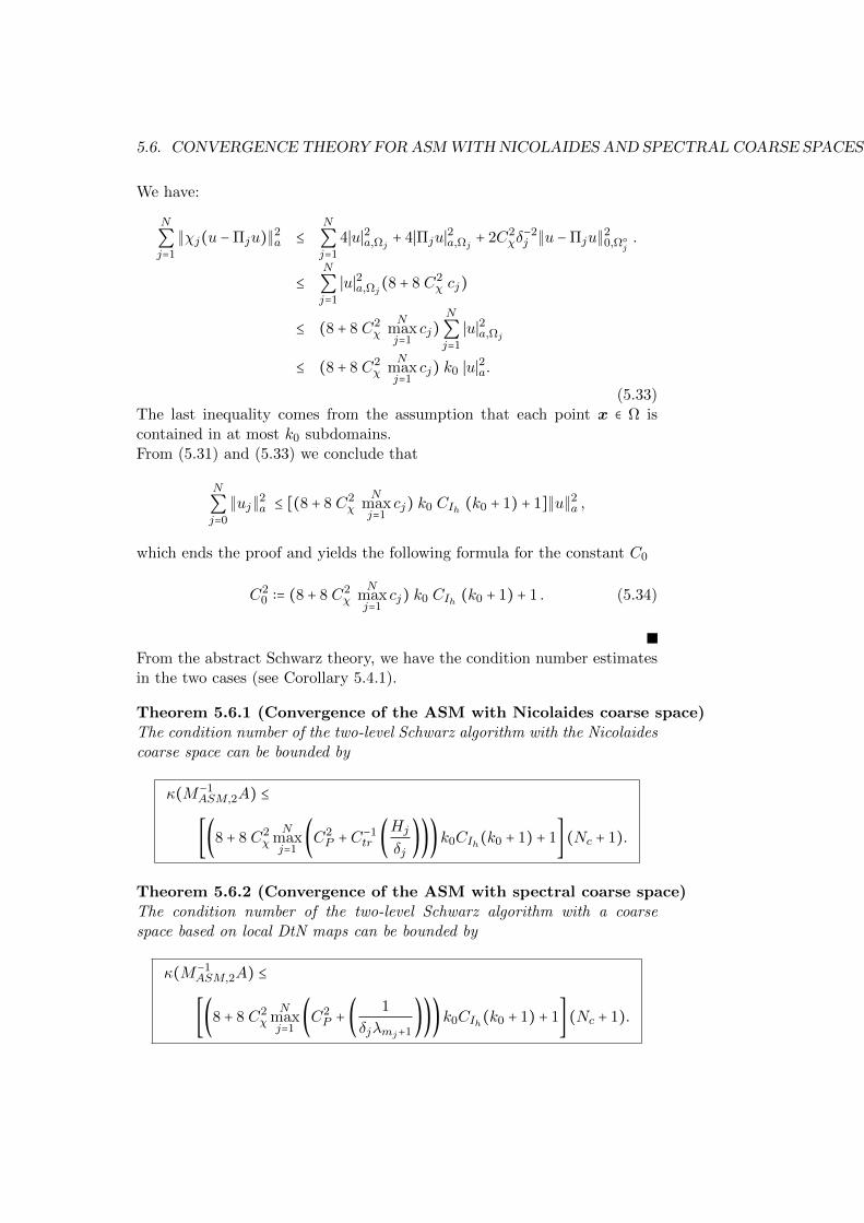
5.6. CONVERGENCE THEORY FORASMWITH NICOLAIDES AND SPECTRAL COARSE SPACES151
We have:
N
∑j=1
∥χj(u −Πju)∥2a ≤
N
∑j=1
4∣u∣2a,Ωj + 4∣Πju∣2a,Ωj + 2C2χδ
−2j ∥u −Πju∥2
0,Ωj.
≤N
∑j=1
∣u∣2a,Ωj(8 + 8 C2χ cj)
≤ (8 + 8 C2χ
Nmaxj=1
cj)N
∑j=1
∣u∣2a,Ωj
≤ (8 + 8 C2χ
Nmaxj=1
cj) k0 ∣u∣2a.(5.33)
The last inequality comes from the assumption that each point x ∈ Ω iscontained in at most k0 subdomains.From (5.31) and (5.33) we conclude that
N
∑j=0
∥uj∥2a ≤ [(8 + 8 C2
χN
maxj=1
cj) k0 CIh (k0 + 1) + 1]∥u∥2a ,
which ends the proof and yields the following formula for the constant C0
C20 ∶= (8 + 8 C2
χN
maxj=1
cj) k0 CIh (k0 + 1) + 1 . (5.34)
From the abstract Schwarz theory, we have the condition number estimatesin the two cases (see Corollary 5.4.1).
Theorem 5.6.1 (Convergence of the ASM with Nicolaides coarse space)The condition number of the two-level Schwarz algorithm with the Nicolaidescoarse space can be bounded by
κ(M−1ASM,2A) ≤
[(8 + 8 C2χ
Nmaxj=1
(C2P +C−1
tr (Hj
δj)))k0CIh(k0 + 1) + 1] (Nc + 1).
Theorem 5.6.2 (Convergence of the ASM with spectral coarse space)The condition number of the two-level Schwarz algorithm with a coarsespace based on local DtN maps can be bounded by
κ(M−1ASM,2A) ≤
[(8 + 8 C2χ
Nmaxj=1
(C2P + ( 1
δjλmj+1)))k0CIh(k0 + 1) + 1] (Nc + 1).

152 CHAPTER 5. THEORY OF TWO-LEVEL ASM
Djk
Xjk
Ωj
Ω0j
Figure 5.3: Assumption on the overlapping region
Remark 5.6.1 Note that, by choosing the number mj of modes per subdo-
main in the coarse space such that λ(j)mj+1 ≥H−1
j , the preconditioned problemusing the coarse space verifies
κ(M−1ASM,2A) ≤
[(8 + 8 C2χ
Nmaxj=1
(C2P + (Hj
δj)))k0CIh(k0 + 1) + 1] (Nc + 1).
Hence, we have the same type of estimate as for the Nicolaides coarse space.An interesting observation is that the bound depends only in an additiveway on the constant CP and on the ratio of subdomain diameter to overlap.
5.7 Functional analysis results
We prove Lemma 5.7.2 that was used to establish estimate (5.22). We startby stating an assumption on the overlapping subregions.
Assumption 5.7.1 We assume that each Ωj , j = 1, . . . ,N , can be subdi-
vided into regions Djk, k = 1, . . . ,Kj (see Figure 5.3), such that diam(Djk) ≂δj and ∣Djk∣ ≂ δdj , and such that, for each k, the (d−1)–dimensional manifold
Xjk ∶= ∂Ωj ∩Djk has the following properties:
(i) ∣Xjk∣ ≂ δd−1j .
(ii)∣Djk ∣
∣Xjk ∣≤ 2δj .
We assume as well that the triangulation Th resolves each of the regions Djk
and each of the manifolds Xjk.
In [161], the following uniform Poincare inequality is proved:

5.8. THEORYOF SPECTRAL COARSE SPACES FOR SCALAR HETEROGENEOUS PROBLEMS153
Lemma 5.7.1 There exists a uniform constant CP > 0, such that the fol-lowing Poincare–type inequality holds for all j = 1, . . . ,N and k = 1, . . . ,Kj:
∥v − vXjk∥0,Djk ≤ CP δj ∣v∣a,Djk , for all v ∈ Vh(Djk).
The constant CP is independent of h and δj.
We then prove the following result:
Lemma 5.7.2 We have
∥u∥20,Ω
j≤ 2C2
P δ2j ∣u∣2a,Ω
j+ 4δj∥u∥2
0,∂Ωj, for all u ∈ Vh(Ω
j).
Proof It follows from Lemma 5.7.1, as well as the triangle and the Cauchy-Schwarz inequalities, that
12∥u∥
20,Djk
≤ ∥u − uXjk∥20,Djk
+ ∥uXjk∥20,Djk
≤ C2P δ
2j ∣u∣2a,Djk +
∣Djk∣∣Xjk∣2
(∫Xjk
u)2
≤ C2P δ
2j ∣u∣2a,Djk +
∣Djk∣∣Xjk∣∫Xjk
u2
≤ C2P δ
2j ∣u∣2a,Djk + 2δj ∥u∥2
0,Xjk.
The final result follows by summing over k = 1, . . . ,Kj .
5.8 Theory of spectral coarse spaces for scalar het-erogeneous problems
The analysis of the spectral coarse space introduced in [147] for highly het-erogeneous Darcy equation
−div(α∇u) = f, in Ω
where α can vary of several orders of magnitude, typically between 1 and106 was analyzed in [63]. A similar but different approach is developed in[84]. These results generalize the classical estimates of overlapping Schwarzmethods to the case where the coarse space is richer than just the kernelof the local operators (which is the set of constant functions) [151], orother classical coarse spaces (cf. [184]). It is particularly well suited tothe small overlap case. In the case of generous overlap, our analysis relieson an assumption on the coefficient distribution that may not be satisfiedfor small scale coefficient variation. This assumption does not seem to benecessary in practice, see also [148] for more extensive numerical results.

154 CHAPTER 5. THEORY OF TWO-LEVEL ASM
The idea of a coarse space based on spectral information that allows toachieve any a priori chosen target convergence rate was developed andimplemented in the spectral AMGe method in [24]. More recently, in theframework of two-level overlapping Schwarz, [84, 83, 147, 148, 70] also buildcoarse spaces for problems with highly heterogeneous coefficients by solvinglocal eigenproblems. However, compared to the earlier works in the AMGcontext the recent papers all focus on generalized eigenvalue problems. Wecan distinguish three sets of methods that all differ by the choice of thebilinear form on the right-hand side of the generalized eigenproblem. In[84, 83], the right-hand side is the local mass matrix, or a “homogenized”version obtained by using a multiscale partition of unity. In [147, 148] theright-hand side corresponds to an L2-product on the subdomain boundary,so that the problem can be reduced to a generalized eigenproblem for theDtN operator on the subdomain boundary. The latest set of papers, [70],uses yet another type of bilinear form on the right-hand side, inspired bytheoretical considerations. In [173], the construction of energy-minimizingcoarse spaces that obey certain functional constraints are used to buildrobust coarse spaces for elliptic problems with large variations in thecoefficients.
All these approaches have their advantages and disadvantages, which dependon many factors, in particular the type of coefficient variation and the sizeof the overlap. When the coefficient variation is on a very small scale manyof the above approaches lead to rather large (and therefore costly) coarsespaces, and it is still an open theoretical question how large the coarse spacewill have to become in each case to achieve robustness for an arbitrarycoefficient variation and how to mitigate this.
Chapter 6
Neumann-Neumann andFETI Algorithms
The last decade has shown, that Neumann-Neumann [13, 132, 125] typeand FETI [81] algorithms, as well as their variants such as BDDC [48] andFETI-DP [78] algorithms, are very efficient domain decomposition methods.Most of the early theoretical and numerical work has been carried out forsymmetric positive definite second order problems, see for example [40, 135,81, 136]. Then, the method was extended to different other problems, likethe advection-diffusion equations [95, 1], plate and shell problems [181] orthe Stokes equations [155, 182].
These methods require pseudo inverses for local Neumann solves which canbe ill-posed either in the formulation of the domain decomposition problemor in the domain decomposition preconditioner. FETI methods are based onthe introduction of Lagrange multipliers on the interfaces to ensure a weakcontinuity of the solution. We present here an alternative formulation of theNeumann-Neumann algorithm with the purpose of simplifying the numericalimplementation. This is made at the expense of minor modifications to theoriginal algorithm while keeping its main features. We start with a historicaland heuristic presentation of these methods.
6.1 Direct and Hybrid Substructured solvers
Neumann-Neumann and FETI methods originated from parallel directsolvers. For a general matrix, direct methods consist in performing itsGauss decomposition into a lower triangular matrix and an upper triangularone, a.k.a. LU decomposition. For a symmetric positive definite matrix, aCholesky decomposition into a lower triangular matrix times its transposeis cheaper (a.k.a. LLT decomposition). In order to benefit from the spar-sity of the matrix arising from a finite element discretization of a partial
155
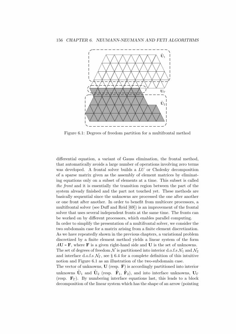
156 CHAPTER 6. NEUMANN-NEUMANN AND FETI ALGORITHMS
U
U1
U2
Figure 6.1: Degrees of freedom partition for a multifrontal method
differential equation, a variant of Gauss elimination, the frontal method,that automatically avoids a large number of operations involving zero termswas developed. A frontal solver builds a LU or Cholesky decompositionof a sparse matrix given as the assembly of element matrices by eliminat-ing equations only on a subset of elements at a time. This subset is calledthe front and it is essentially the transition region between the part of thesystem already finished and the part not touched yet. These methods arebasically sequential since the unknowns are processed the one after anotheror one front after another. In order to benefit from multicore processors, amultifrontal solver (see Duff and Reid [69]) is an improvement of the frontalsolver that uses several independent fronts at the same time. The fronts canbe worked on by different processors, which enables parallel computing.In order to simplify the presentation of a multifrontal solver, we consider thetwo subdomain case for a matrix arising from a finite element discretization.As we have repeatedly shown in the previous chapters, a variational problemdiscretized by a finite element method yields a linear system of the formAU = F, where F is a given right-hand side and U is the set of unknowns.The set of degrees of freedom N is partitioned into interior d.o.f.s N1 and N2
and interface d.o.f.s NΓ, see § 6.4 for a complete definition of this intuitivenotion and Figure 6.1 as an illustration of the two-subdomain case.The vector of unknowns, U (resp. F) is accordingly partitioned into interior
unknownsU1 and
U2 (resp.
F1,
F2), and into interface unknowns, UΓ
(resp. FΓ). By numbering interface equations last, this leads to a blockdecomposition of the linear system which has the shape of an arrow (pointing

6.1. DIRECT AND HYBRID SUBSTRUCTURED SOLVERS 157
down to the right):
⎛⎜⎝
A11 0 A1Γ
0 A22 A2Γ
AΓ1 AΓ2 AΓΓ
⎞⎟⎠
⎛⎜⎜⎝
U1U2
UΓ
⎞⎟⎟⎠=⎛⎜⎜⎝
F1F2
FΓ
⎞⎟⎟⎠. (6.1)
A simple computation shows that we have a block factorization of matrix A
A =⎛⎜⎝
I0 I
AΓ1A−111 AΓ2A
−122 I
⎞⎟⎠
⎛⎜⎝
A11
A22
S
⎞⎟⎠
⎛⎜⎝
I 0 A−111A1Γ
I A−122A2Γ
I
⎞⎟⎠. (6.2)
Here, the matrix
S ∶= AΓΓ −AΓ1A−111A1Γ −AΓ2A
−122A2Γ (6.3)
is a Schur complement matrix and it is dense. It corresponds to an elimina-
tion of the interior unknownsUi, i = 1,2.
From (6.2) we can see that the inverse of A can be easily computed from itsfactorization
A−1 =⎛⎜⎝
I 0 −A−111A1Γ
I −A−122A2Γ
I
⎞⎟⎠
⎛⎜⎝
A−111
A−122
S−1
⎞⎟⎠
⎛⎜⎝
I0 I
−AΓ1A−111 −AΓ2A
−122 I
⎞⎟⎠.
(6.4)Note that in practice, the three matrices A−1
11 , A−122 and S−1 are never evalu-
ated explicitly. From the above formula, it appears that applying A−1 to theright-hand side F is equivalent to solving linear systems for the three abovematrices which can be done by factorizing them. The parallelism comesfrom the fact that matrices A11 and A22 can be factorized concurrently. Wesay we advance two fronts in parallel. Once it is done, matrix S can becomputed and then factorized.By considering more than two fronts and recursive variants, it is possibleto have numerical efficiency for one or possibly two dozens of cores andproblems of size one or two millions of unknowns in two dimensions andhundreds of thousands degrees of freedom in three dimensions. Althoughthese figures improve over time, it is generally accepted that purely directsolvers cannot scale well on large parallel platforms. The bottleneck comesfrom the fact that S is a full matrix which is costly to compute andfactorize. This is unfortunate since direct solvers have the advantage overiterative solvers to be very predictable, reliable and easy to integrate viathird-party libraries. There is thus a great amount of effort in developinghybrid direct/iterative solvers that try to take advantage of the two worlds.
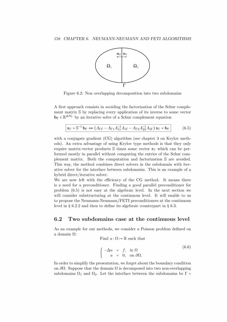
158 CHAPTER 6. NEUMANN-NEUMANN AND FETI ALGORITHMS
n1n2
Figure 6.2: Non overlapping decomposition into two subdomains
A first approach consists in avoiding the factorization of the Schur comple-ment matrix S by replacing every application of its inverse to some vectorbΓ ∈ R#NΓ by an iterative solve of a Schur complement equation
xΓ = S−1 bΓ ⇔ (AΓΓ −AΓ1A−111A1Γ −AΓ2A
−122A2Γ)xΓ = bΓ (6.5)
with a conjugate gradient (CG) algorithm (see chapter 3 on Krylov meth-ods). An extra advantage of using Krylov type methods is that they onlyrequire matrix-vector products S times some vector rΓ which can be per-formed mostly in parallel without computing the entries of the Schur com-plement matrix. Both the computation and factorization S are avoided.This way, the method combines direct solvers in the subdomain with iter-ative solver for the interface between subdomains. This is an example of ahybrid direct/iterative solver.We are now left with the efficiency of the CG method. It means thereis a need for a preconditioner. Finding a good parallel preconditioner forproblem (6.5) is not easy at the algebraic level. In the next section wewill consider substructuring at the continuous level. It will enable to usto propose the Neumann-Neumann/FETI preconditioners at the continuouslevel in § 6.2.2 and then to define its algebraic counterpart in § 6.3.
6.2 Two subdomains case at the continuous level
As an example for our methods, we consider a Poisson problem defined ona domain Ω:
Find u ∶ Ω↦ R such that
−∆u = f, in Ωu = 0, on ∂Ω.
(6.6)
In order to simplify the presentation, we forget about the boundary conditionon ∂Ω. Suppose that the domain Ω is decomposed into two non-overlappingsubdomains Ω1 and Ω2. Let the interface between the subdomains be Γ =

6.2. TWO-SUBDOMAINS AT THE CONTINUOUS LEVEL 159
Ω1 ∩ Ω2, and (ni)i=1,2 be the outward normal to the artificial boundary Γcorresponding to Ω1,2.It is known that u1 (resp. u2) is the restriction of the solution to (6.6) tosubdomain Ω1 (resp. Ω2) if and only if:
⎧⎪⎪⎪⎪⎪⎪⎪⎪⎨⎪⎪⎪⎪⎪⎪⎪⎪⎩
−∆ui = f, in Ωi, i = 1,2 ,
u1 = u2, on Γ ,
∂u1
∂n1+ ∂u2
∂n2= 0, on Γ .
(6.7)
In other words, the local functions must satisfy the Poisson equation in thesubdomains and match at the interface. Since the Poisson equation is ascalar second order partial differential equations, we have two continuityequations on the interface one for the unknown and the second one for thenormal derivatives. Recall that for overlapping subdomains, a matchingcondition of the unknown on the interfaces is sufficient, see chapter 1 onSchwarz methods.
6.2.1 Iterative Neumann-Neumann and FETI algorithms
In this section we will write iterative methods for solving eq. (6.7). They arevery naturally derived from (6.7) by relaxing then correcting the continuityrelations on the interface. When the flux continuity is relaxed, we obtainwhat is called a Neumann-Neumann method and when the continuity onthe Dirichlet data is relaxed we obtain an iterative version of the FETIalgorithm. Both Neumann-Neumann and FETI methods will be investigatedat the algebraic level in the sequel in § 6.3.
Definition 6.2.1 (Iterative Neumann-Neumann algorithm) Let unidenote an approximation to the solution u in a subdomain Ωi, i = 1,2 atthe iteration n. Starting from an initial guess u0
i , the Neumann-Neumanniteration computes the approximation (un+1
1 , un+12 ) from (un1 , un2) by solving
a local Dirichlet problem with a continuous data at the interface
⎧⎪⎪⎪⎪⎨⎪⎪⎪⎪⎩
−∆(un+12
i ) = f, in Ωi,
un+ 1
2i = 1
2(unj + uni ), on Γ.
(6.8)
followed by a correction for the jump of the fluxes on the interface
⎧⎪⎪⎪⎪⎪⎪⎪⎨⎪⎪⎪⎪⎪⎪⎪⎩
−∆(en+1i ) = 0, in Ωi,
∂en+1i
∂ni= −1
2
⎛⎜⎝∂u
n+ 12
1
∂n1+ ∂u
n+ 12
2
∂n2
⎞⎟⎠
on Γ.(6.9)

160 CHAPTER 6. NEUMANN-NEUMANN AND FETI ALGORITHMS
l L0
x
u01
u02
u122u
121
u11 u1
2
Figure 6.3: First iteration of a Neumann-Neumann algorithm
The next iteration is then given by
un+1i = un+
12
i + en+1i , i = 1,2. (6.10)
The rationale for the first step (6.8) is to satisfy the Poisson equation in thesubdomains while ensuring the continuity of the solution on the interface Γ.After this step, the solution is continuous on the interfaces but the fluxesmay not match. The jump on the fluxes is corrected after (6.10). On Γ wehave
∂un+11
∂n1+ ∂u
n+12
∂n2= ∂
∂n1(un+
12
1 + en+11 ) + ∂
∂n2(un+
12
2 + en+12 )
=∂u
n+ 12
i
∂ni− 1
2
⎛⎜⎝∂u
n+ 12
1
∂n1+ ∂u
n+ 12
2
∂n2
⎞⎟⎠+ ∂u
n+ 12
2
∂n2− 1
2
⎛⎜⎝∂u
n+ 12
1
∂n1+ ∂u
n+ 12
2
∂n2
⎞⎟⎠= 0.
Then, functions un+1i , i = 1,2 may not match on the interface. In order to
correct this misfit correction (6.8) is applied again and so on.
Definition 6.2.2 (Iterative FETI algorithm) Let uni denote an approx-imation to the solution u in a subdomain Ωi, i = 1,2 at the iteration n.Starting from the initial guess u0
i , FETI iteration computes the approxima-tion (un+1
1 , un+12 ) from (un1 , un2) by first correcting the jump of the normal
derivatives on the interface
⎧⎪⎪⎪⎪⎪⎪⎨⎪⎪⎪⎪⎪⎪⎩
−∆(un+12
i ) = f, in Ωi,
∂un+ 1
2i
∂ni= ∂uni
∂ni− 1
2(∂u
n1
∂n1+ ∂u
n2
∂n2) on Γ.
(6.11)

6.2. TWO-SUBDOMAINS AT THE CONTINUOUS LEVEL 161
and then the discontinuity of the solution:
⎧⎪⎪⎪⎨⎪⎪⎪⎩
−∆(en+1i ) = 0, in Ωi,
en+1i = 1
2(un+ 1
2j − un+
12
i ) on Γ for j ≠ i .(6.12)
The next iteration is then given by:
un+1i = un+
12
i + en+1i , ı = 1,2, . (6.13)
6.2.2 Substructured reformulations
It consists in reformulating the algorithms from the Definitions 6.2.1 and6.2.2 in term of the interface unknowns on Γ and operators acting on theseinterface unknowns.
Definition 6.2.3 (Interface operators for the Neumann-Neumann algorithm)Let the operators S1,S2 be defined as
Si(uΓ, f) ∶=∂ui∂ni
, i = 1,2, (6.14)
where ui solve the local problems
⎧⎪⎪⎨⎪⎪⎩
−∆ui = f, in Ωi,
ui = uΓ, on Γ.(6.15)
Let also S be defined as the operator
S(uΓ, f) ∶= S1(uΓ, f) + S2(uΓ, f) =∂u1
∂n1+ ∂u2
∂n2(6.16)
which quantifies the jump of the normal derivative at the interface. Definealso operator T by
T (gΓ) ∶=1
2(S−1
1 (gΓ,0) + S−12 (gΓ,0))
1
2= 1
4(e1 ∣Γ + e2 ∣Γ) . (6.17)
where the ei ∣Γ ∶= S−1i (uΓ,0) are obtained by solving Neumann local problems
⎧⎪⎪⎪⎪⎨⎪⎪⎪⎪⎩
−∆ei = 0, in Ωi,
∂ei∂ni
= gΓ on Γ .(6.18)
With this notations, steps (6.9)-(6.10) can be re-written in terms of interfaceunknowns.

162 CHAPTER 6. NEUMANN-NEUMANN AND FETI ALGORITHMS
Lemma 6.2.1 (Neumann-Neumann interface iterative version)The substructured counterpart of the Neumann-Neumann algorithm fromDefinition 6.2.1 will compute un+1
Γ from unΓ by the following iteration
un+1Γ = unΓ − (T S) (unΓ, f) . (6.19)
This defines what we call the iterative interface version of the Neumann-Neumann algorithm.
In order to accelerate this fixed point method by a Krylov algorithm, weidentify this equation with formula (3.3) of chapter 3 on Krylov methods.It is then more efficient to use a Krylov method to solve the substructuredproblem.
Definition 6.2.4 (Substructuring formulation for Neumann-Neumann)The substructured formulation of the Neumann-Neumann iteration consistsin solving, typically by a PCG algorithm, the interface problem
Find uΓ ∶ Γ→ R such thatS(.,0)(uΓ) = −S(0, f)
(6.20)
preconditioned by the linear operator T .
It can be checked that both operators S(.,0) and T are symmetric positivedefinite and thus the preconditioned conjugate gradient algorithm (PCG)can be used. Moreover the action of both operators S(.,0) and T canbe computed mostly in parallel. This very popular preconditioner for theoperator S(0, .) was proposed in [13].
Remark 6.2.1 There are at least three point of views that indicate the rel-evance of this simply derived preconditioner
• Symmetry considerations In the special case where Γ is a symmetryaxis for domain Ω (see fig. 6.2), we have S−1
1 (.,0) = S−12 (.,0) and thus
T is an exact preconditioner for S(.,0) since it is easy to check that(T S)(.,0) = Id.
• Mechanical interpretation The unknown u may be the temperaturein domain Ω that obeys a Poisson equation with a source term f .Operator S(.,0) acts on temperature on the interface and returns aheat flux across the interface. A good preconditioner should act on aheat flux and return a temperature. If the Poisson equation is replacedby the elasticity system, the notion of temperature is replaced by thatof displacement and that of the normal flux by that of a normal stressto the interface (or a force).

6.2. TWO-SUBDOMAINS AT THE CONTINUOUS LEVEL 163
• Functional analysis considerations A classical setting for the in-terface operator S(.,0) is to define it as continuous linear operator
from the Sobolev space H1/200 (Γ) with values in H−1/2(Γ). Operator
T is a continuous linear operator from H−1/2(Γ) with values into
H1/200 (Γ). Thus, the preconditioned operator T S(.,0) is a contin-
uous from H1/200 (Γ) into itself. Any meaningful discretizations of this
product of operators is then expected to lead to a condition numberindependent of the mesh size.
It is possible to consider the Neumann-Neumann preconditioner the otherway round. The unknown is the flux at the interface between the subdo-mains. In this case we will obtain the FETI iterative algorithm. Note thatdue to the opposite signs of the outward normal ni to subdomain Ωi, thedefinition of the normal flux is arbitrary up to a flip of sign. In this casewe will have to define first interface operators acting on fluxes (or dual vari-ables) which will be preconditioned by operators acting on “displacements”(or the primal variables).
Definition 6.2.5 (Interface operator for the FETI algorithm) Letλ be a function that lives on the interface Γ and Tfeti be a function of fand λ defined by
Tfeti(λ, f) ∶= v2 − v1 (6.21)
where the vi are solutions of the Neumann BVP’s (i = 1,2):
⎧⎪⎪⎪⎪⎨⎪⎪⎪⎪⎩
−∆vi = f in Ωi,
∂vi∂ni
= (−1)iλ on Γ.(6.22)
This function quantifies the jump of the solutions across the interface.
Note that we have Tfeti(λ,0) = 4T (λ) (defined by (6.17)), which means theoperator
Sfeti =1
2S(.,0)1
2(6.23)
is a good preconditioner for Tfeti. By using a similar argument as in thecase of the Neumann-Neumann algorithm, we can state the following result.
Lemma 6.2.2 (FETI interface iterative version) The substructuredcounterpart of the FETI algorithm from Definition 6.2.2 will compute λn+1
Γ
from λnΓ by the following iteration
λn+1Γ = λnΓ − (Sfeti Tfeti) (λnΓ, f) . (6.24)
This defines what we call the iterative interface version of the FETI algo-rithm.
164 CHAPTER 6. NEUMANN-NEUMANN AND FETI ALGORITHMS
In order to accelerate this fixed point method by a Krylov algorithm, weidentify this equation with formula (3.3) of chapter 3 on Krylov methods.It is then more efficient to use a Krylov method to solve the substructuredproblem.
Definition 6.2.6 (Substructuring formulation for FETI) The sub-structured formulation of the FETI iteration iteration consists in solvingthe interface problem
Find λ ∶ Γ↦ R such thatTfeti(λ,0) = −Tfeti(0, f) .
(6.25)
preconditioned by the operator Sfeti which involves the solving in parallel ofa Dirichlet boundary value problem in each subdomain.
Problem (6.25) is solved by a PCG algorithm with (6.23) as a preconditioner.This approach has been developed in [80, 37, 123].
6.2.3 FETI as an optimization problem
As explained in the sequel, equation (6.25) can be interpreted as the dualproblem of a minimization problem under equality constraints. First notethat the original boundary value problem (6.6) is equivalent to the followingminimization problem:
minu∈H1(Ω)
JΩ(u), JΩ(u) ∶= 1
2∫
Ω∣∇u∣2 − ∫
Ωf u (6.26)
where H1(Ω) is the Sobolev space of functions that are square integrable andtheir derivatives are square integrable as well. In order to introduce domaindecomposition methods, we make use of a functional analysis result thatproves that space H1(Ω) is isomorphic to the “domain decomposed space”(local H1 functions with Dirichlet traces continuous at the interface):
H1(Ω1,Ω2) ∶= (u1, u2) ∈H1(Ω1) ×H1(Ω2)/ u1 = u2 on Γ ,see e.g. [14] or [30]. This allows the “splitting” of the functional of optimiza-tion problem (6.26) into local contributions constrained by the continuitycondition at the interface. We have thus the following
Lemma 6.2.3 (Dual optimization problem) Minimization prob-lem (6.26) is equivalent to
min(u1,u2)∈H1(Ω1,Ω2)
J(u1, u2) ∶= min(u1,u2)∈H1(Ω1,Ω2)
JΩ1(u1) + JΩ(u2)
= minu1 ∈H1(Ω1)u2 ∈H2(Ω2)u1 = u2,on Γ
1
2∫
Ω1
∣∇u1∣2 +1
2∫
Ω2
∣∇u2∣2 − ∫Ω1
f u1 − ∫Ω2
f u2.
(6.27)

6.3. TWO SUBDOMAINS CASE AT THE ALGEBRAIC LEVEL 165
Note that a Lagrangian function of this constrained optimization problemcan be written as
L(u1, u2, λ) ∶= JΩ1(u1) + JΩ(u2) + ∫Γλ (u1 − u2) .
By computing the differential of L with respect to the ui’s we get that thecritical points satisfy weakly the local boundary value problems, on one hand
⎧⎪⎪⎪⎪⎨⎪⎪⎪⎪⎩
−∆ui = f, in Ω1
∂ui∂ni
= (−1)iλ, on Γ(6.28)
and the continuity conditionu1 = u2 (6.29)
on the other hand. We see that (6.28) and (6.29) can be rewritten equiva-lently by using the relations (6.21) and (6.22) from Definition 6.2.5,
Tfeti(λ, f) = 0
which is equivalent to the substructured formulation (6.25).
6.3 Two subdomains case at the algebraic level
The goal of this section is to write the algebraic counterpart of the algorithmsdefined in the previous section at the continuous level. This way, we shall beable to propose a good preconditioner for the algebraic Schur complementequation (6.5). This will be done in a finite element framework.As we have seen in the beginning of this chapter, a variational problemdiscretized by a finite element method yields a linear system of the formAU = F, where F is a given right-hand side and U is the set of unknowns.The set of degrees of freedom N is decomposed into interior d.o.f.s N1 andN2 and interface d.o.f.sNΓ, see § 6.4 for a complete definition of this intuitivenotion and Figure 6.1 as an illustration of the two-subdomain case.The vector of unknowns U (resp. F) is decomposed into interior unknownsU1 and
U2 (resp.
F1,
F2), and into interface unknowns, UΓ (resp. FΓ). By
numbering interface equations last, we obtain a block decomposition of thelinear system which has the shape of an arrow (pointing down to the right):
⎛⎜⎝
A11 0 A1Γ
0 A22 A2Γ
AΓ1 AΓ2 AΓΓ
⎞⎟⎠
⎛⎜⎜⎝
U1U2
UΓ
⎞⎟⎟⎠=⎛⎜⎜⎝
F1F2
FΓ
⎞⎟⎟⎠. (6.30)
The algebraic counterpart of the continuous substructured problem (6.20)
amounts simply to an elimination of the interior unknownsUi, i = 1,2 in
166 CHAPTER 6. NEUMANN-NEUMANN AND FETI ALGORITHMS
(6.30) which leads to a Schur complement equation:
S(UΓ,F) ∶= (AΓΓ −AΓ1A−111A1Γ −AΓ2A
−122A2Γ) (UΓ)
−(FΓ −AΓ1A−111
F1 −AΓ2A
−122
F2) = 0
(6.31)
The natural algebraic form of operator S by (6.16) is thus defined by Sin the above formula. In order to find the algebraic counterparts of thecontinuous preconditioner T (eq.(6.17)) and thus of the continuous opera-tors Si (eq.(6.14)), i = 1,2 we need somehow to split the operator into twocontributions coming from the subdomains.For this purpose, we first of all note that there is a natural decomposi-tion of AΓΓ = (aklΓΓ)k,l∈NΓ
into its contribution coming from each subdomainAΓΓ = A1
ΓΓ + A2ΓΓ. More precisely, let k, l be the indices of two degrees of
freedom on the interface associated with two basis functions φk and φl. Thecorresponding entry aklΓΓ can be decomposed into a sum aklΓΓ = a1,kl
ΓΓ + a2,klΓΓ ,
where
ai,klΓΓ = ∫Ωi∇φk∇φl, i = 1,2.
In the same spirit, we define for i = 1,2 and k ∈ NΓ:
f(i),kΓ ∶= ∫
Ωif φk
and F(i)Γ ∶= (f (i),k
Γ )k∈NΓ. In order to make things simple, we have only
considered the Poisson problem. Other partial differential equations such asthe elasticity equations can be handled in the same manner.Finally, we have a decomposition of matrix AΓΓ into
AΓΓ = A(1)ΓΓ +A(2)
ΓΓ (6.32)
and of FΓ into
FΓ = F(1)Γ +F
(2)Γ .
We can infer that for each domain i = 1,2, the local operators
Si(UΓ,F) ∶= (A(i)ΓΓ −AΓiA
−1ii AiΓ) (UΓ) − (F(i)
Γ −AΓiA−1ii
Fi) .
are discretizations of the continuous operators Si, i = 1,2 and let Si ∶= Si(.,0)be local Schur complements. Note that from (6.32) we have as in the con-tinuous case that:
S(UΓ,F) = S1(UΓ,F) + S2(UΓ,F) and S = S1 + S2.
Coming back to the substructuring, we obtain now natural a very naturaldefinition.

6.3. TWO SUBDOMAINS CASE AT THE ALGEBRAIC LEVEL 167
Definition 6.3.1 (Substructuring formulation for Neumann-Neumann)Since S = S(⋅,0), the substructured formulation reads
Find UΓ ∈ R#NΓ , such thatS(UΓ) = −S(0,F) (6.33)
The preconditioner T analogous to (6.17) is the weighted sum:
T ∶= 1
2(S1(.,0)−1 + S2(.,0)−1)1
2. (6.34)
The action of Si(.,0)−1 on some interface vector gΓ, vi,Γ = Si(.,0)−1gΓ canbe computed by solving the discretized Neumann problem related to (6.18):
(Aii AiΓ
AΓi A(i)ΓΓ
)(vivi,Γ
) =⎛⎝
0
gΓ
⎞⎠. (6.35)
To sum up, the Neumann-Neumann method consists in solving for UΓ theSchur complement equation (6.31) or (6.33) by the PCG method using oper-ator T (6.34) as a preconditioner. At convergence, the algorithm will providethe interface values. Interior values in each subdomain can be computed bysolving local Dirichlet problems:
AiiUi=
F i −AiΓUΓ . (6.36)
Parallelism is natural since all these steps can mostly be computed concur-rently on two processors. Matrix-vector products with operators S and Tare both defined as sums of local computations and are therefore essentiallyparallel with a very high ratio of local computations over data transfer be-tween processors. As for the step defined by equation (6.36), it is purelyparallel.
As in the continuous case, it is possible to invert the role of the Neumannand Dirichlet problems and thus obtain the FETI algorithm.
Definition 6.3.2 (FETI interface operator) Let the operator
Tfeti ∶ R#NΓ ×R#N Ð→ R#NΓ
be defined for some λ ∈ R#NΓ and F ∈ R#N as
Tfeti(λ,F) ∶= V2,Γ −V1,Γ ,
where (Vi, Vi,Γ) are the solutions of
(Aii AiΓ
AΓi A(i)ΓΓ
)(Vi
Vi,Γ
) =⎛⎝
Fi
F(i)Γ + (−1)iλ
⎞⎠. (6.37)
168 CHAPTER 6. NEUMANN-NEUMANN AND FETI ALGORITHMS
It can be checked that Tfeti(λ,0) = 4T. We can infer from this that since T isa good preconditioner for S, 1
4S is a good preconditioner for Tfeti. This leadsto the following definition of the discrete FETI substructured formulation.
Definition 6.3.3 (Substructuring formulation for FETI) The sub-structured formulation of the FETI algorithm reads
Find λ ∈ R#NΓ , such thatTfeti(λ,0) = −Tfeti(0,F) .
This problem is solved by the PCG algorithm, using the operator
1
2S
1
2
as a preconditioner.
This approach has been developed in [80, 37, 123].
6.3.1 Link with approximate factorization
Following [175], we will establish a connection between the Neumann-Neumann algorithm and a block approximate factorization of the originalsystem (6.30). Recall first that an exact block factorization of matrix A isgiven by equation (6.2) so that its inverse is given by the formula in equation(6.4)
A−1 =⎛⎜⎝
I 0 −A−111A1Γ
I −A−122A2Γ
I
⎞⎟⎠
⎛⎜⎝
A−111
A−122
S−1
⎞⎟⎠
⎛⎜⎝
I0 I
−AΓ1A−111 −AΓ2A
−122 I
⎞⎟⎠.
This suggests the approximation M−1 ≃ A−1 of the inverse, which naturallyprovides a preconditioner
M−1 ∶=⎛⎜⎝
I 0 −A−111A1Γ
I −A−122A2Γ
I
⎞⎟⎠
⎛⎜⎝
A−111
A−122
T
⎞⎟⎠
⎛⎜⎝
I0 I
−AΓ1A−111 −AΓ2A
−122 I
⎞⎟⎠.
(6.38)where T is given by (6.34). A direct computation shows that the precondi-tioned system M−1A has the following form:
M−1A =⎛⎜⎝
I 0 00 I 00 0 TS
⎞⎟⎠
Due to the properties of matrices S and T we can state some remarkablefeatures.

6.4. MANY SUBDOMAINS CASE 169
Figure 6.4: Non overlapping geometric partition
Remark 6.3.1 This preconditioner has a few properties:
• In the case of exact solves in the subdomains, that is for the computa-tion of the exact factorization of Aii, the application of this precondi-tioner is equivalent to that of the Schur complement approach, exceptthat it is performed at global level.
• Inexact solvers can be used in the subdomains since the application ofM−1 requires the repeated application of A−1
ii .
• The preconditioner is symmetric and this symmetry can be preservedin the case of inexact solves, provided that the same inexact solves areused in the first and the last terms of (6.38).
• The bad news is that even if we have the spectral equivalence of thepreconditioner with the diagonal blocks A−1
ii , M−1 is not necessarilyspectrally equivalent to matrix A. Whereas with overlapping Schwarzmethods when the local subdomain solvers are replaced by a spectrallyequivalent solver the convergence behavior of the ASM is asymptoticallyequivalent to that of ASM with exact solvers, see [175].
6.4 Many subdomains case
In a finite element setting, the computational domain is the union of elementsof the finite element mesh Th. A geometric partition of the computationaldomain is natural. Here again, graph partitioning can be used by firstmodeling the finite element mesh by a graph, and then partitioning it intoN parts, see Figure 6.4.As in section 1.3.2, we define a partition of unity for the non overlappingdecomposition of the domain Ω into subdomains Ωi, i = 1, . . . ,N . We recall

170 CHAPTER 6. NEUMANN-NEUMANN AND FETI ALGORITHMS
that it corresponds to an overlapping decomposition of the set of d.o.f.sN since some basis functions have a support that intersects two or moresubdomains. Let φkk∈N be a basis of the finite element space. For 1 ≤ i ≤N , we define
Ni ∶= k ∈ N ∶ supp (φk) ∩Ωi ≠ ∅the set of degrees of freedom whose associated basis function intersects sub-domain Ωi. For each degree of freedom k ∈ N , let
µk ∶= #j ∶ 1 ≤ j ≤ N and k ∈ Nj
be the number of subdomains that “interact” with function φk. For exam-ple, for a P1 finite element method and an interface point shared by twosubdomains, we have µk = 2. If the point is a cross point shared by foursubdomains, we have µk = 4.The global set of d.o.f’s can be decomposed into unknowns interior to sub-domains Ωi, 1 ≤ i ≤ N :
N i∶= k ∈ Ni/ µk = 1
and the set of interface unknowns, also called the skeleton, defined as:
NΓ ∶= k ∈ N / µk > 1 .
LetRi and RΓ be the restriction boolean matrices from the global set N
to subsetsN i and NΓ. For U ∈ R#N , let
Ui∶=
Ri U = (Uk)
k∈N i
be the set
of interior degrees of freedom of subdomain Ωi and UΓ ∶= RΓU = (Uk)k∈NΓ
denote the set of interface degrees of freedom. Note that the sets (N i)1≤i≤N
and NΓ form a partition of N
N = (N
⋃i=1
N i)⋃NΓ.
For a finite element discretization of partial differential equations, the matrixhas a sparse structure:
Ri A
Rj
T= 0, for i ≠ j .
If the skeleton unknowns are numbered last, the corresponding block formof the global problem is thus:
⎛⎜⎜⎜⎜⎜⎜⎝
A11 0 ⋯ 0 A1Γ
0 A22 ⋮ A2Γ
⋮ 0 ⋱ 0 ⋮0 0 ANN ANΓ
AΓ1 AΓ2 ⋯ AΓN AΓΓ
⎞⎟⎟⎟⎟⎟⎟⎠
⎛⎜⎜⎜⎜⎜⎜⎜⎝
U1U2
⋮UN
UΓ
⎞⎟⎟⎟⎟⎟⎟⎟⎠
=
⎛⎜⎜⎜⎜⎜⎜⎜⎝
F1F2
⋮FN
FΓ
⎞⎟⎟⎟⎟⎟⎟⎟⎠
(6.39)
6.4. MANY SUBDOMAINS CASE 171
As in the two-subdomain case for matrix (6.1), it has an arrow shape whichallows a multifrontal direct factorization.In order to define a Neumann-Neumann preconditioner for the substructuredproblem
SUΓ = FΓ −N
∑i=1
AΓiA−1ii
Fi, where S ∶= AΓΓ −
N
∑i=1
AΓiA−1ii AiΓ , (6.40)
we make use of the decomposition induced on the skeleton NΓ by the geo-metrical domain decomposition. We have thus the following decompositionof the skeleton:
NΓ = ⋃1≤i≤N
NΓi .
where the set of indices of interface unknowns of subdomain Ωi is
NΓi ∶= k ∈ Ni/ µk > 1 = NΓ ∩Ni 1 ≤ i ≤ N.
Let RΓi be the restriction Boolean matrix from the skeleton NΓ to NΓi . Fora vector of skeleton d.o.f. UΓ ∈ R#NΓ , let UΓi ∶= RΓiUΓ = (UΓk)k∈NΓi
denotethe set of interface degrees of freedom of subdomain Ωi.Let DΓi be a diagonal matrix of size R#NΓi ×R#NΓi whose entries are
(DΓi)kk ∶=1
µk, ∀k ∈ NΓi .
We have clearly partition of unity on the skeleton:
N
∑i=1
RTΓiDΓiRΓi = IdΓ .
In order to define a Neumann-Neumann preconditioner for (6.40), we firstdecompose AΓΓ into its local contributions coming from the subdomains:
AΓΓ =N
∑i=1
A(i)ΓΓ
as it was done in the two subdomain case in eq. (6.32). More precisely fora Poisson problem, let k, l be the indices of two degrees of freedom on theinterface associated with two basis functions φk and φl. The correspondingentry aklΓΓ can be decomposed into a sum ai,klΓΓ , where
ai,klΓΓ = ∫Ωi∇φk∇φl, i = 1, . . . ,N .
This yields a decomposition of S:
S =N
∑i=1
Si, Si ∶= A(i)ΓΓ −AΓiA
−1ii AiΓ . (6.41)
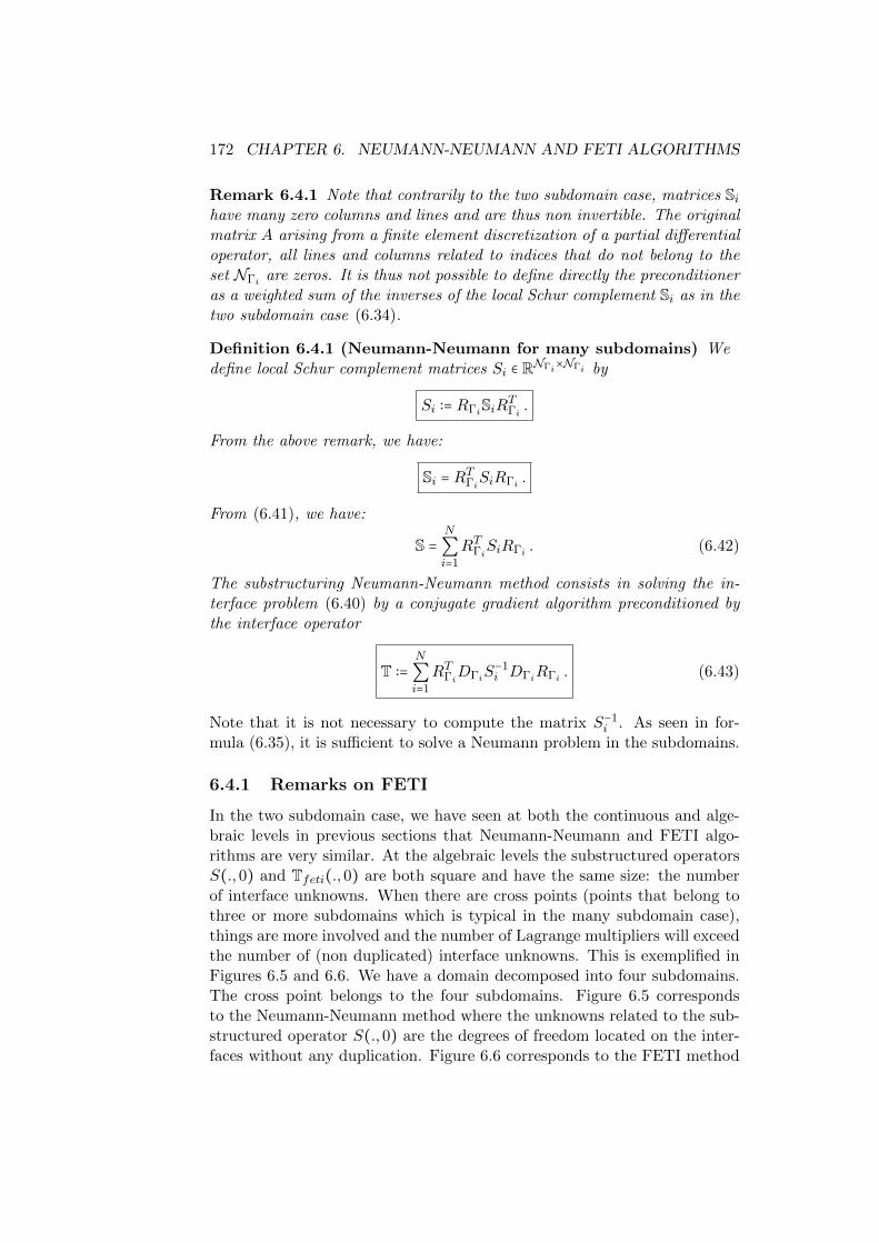
172 CHAPTER 6. NEUMANN-NEUMANN AND FETI ALGORITHMS
Remark 6.4.1 Note that contrarily to the two subdomain case, matrices Sihave many zero columns and lines and are thus non invertible. The originalmatrix A arising from a finite element discretization of a partial differentialoperator, all lines and columns related to indices that do not belong to theset NΓi are zeros. It is thus not possible to define directly the preconditioneras a weighted sum of the inverses of the local Schur complement Si as in thetwo subdomain case (6.34).
Definition 6.4.1 (Neumann-Neumann for many subdomains) Wedefine local Schur complement matrices Si ∈ RNΓi
×NΓi by
Si ∶= RΓiSiRTΓi .
From the above remark, we have:
Si = RTΓiSiRΓi .
From (6.41), we have:
S =N
∑i=1
RTΓiSiRΓi . (6.42)
The substructuring Neumann-Neumann method consists in solving the in-terface problem (6.40) by a conjugate gradient algorithm preconditioned bythe interface operator
T ∶=N
∑i=1
RTΓiDΓiS−1i DΓiRΓi . (6.43)
Note that it is not necessary to compute the matrix S−1i . As seen in for-
mula (6.35), it is sufficient to solve a Neumann problem in the subdomains.
6.4.1 Remarks on FETI
In the two subdomain case, we have seen at both the continuous and alge-braic levels in previous sections that Neumann-Neumann and FETI algo-rithms are very similar. At the algebraic levels the substructured operatorsS(.,0) and Tfeti(.,0) are both square and have the same size: the numberof interface unknowns. When there are cross points (points that belong tothree or more subdomains which is typical in the many subdomain case),things are more involved and the number of Lagrange multipliers will exceedthe number of (non duplicated) interface unknowns. This is exemplified inFigures 6.5 and 6.6. We have a domain decomposed into four subdomains.The cross point belongs to the four subdomains. Figure 6.5 correspondsto the Neumann-Neumann method where the unknowns related to the sub-structured operator S(.,0) are the degrees of freedom located on the inter-faces without any duplication. Figure 6.6 corresponds to the FETI method
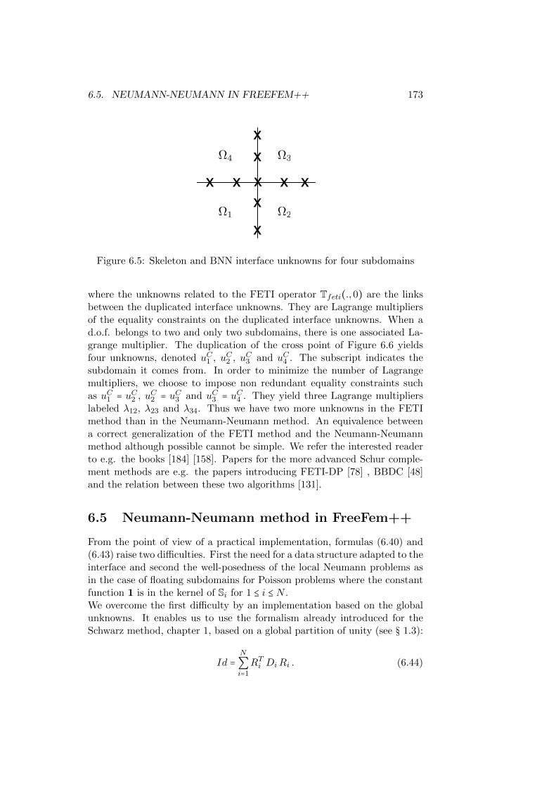
6.5. NEUMANN-NEUMANN IN FREEFEM++ 173
xx xxx
xx
x x1
4 3
2
Figure 6.5: Skeleton and BNN interface unknowns for four subdomains
where the unknowns related to the FETI operator Tfeti(.,0) are the linksbetween the duplicated interface unknowns. They are Lagrange multipliersof the equality constraints on the duplicated interface unknowns. When ad.o.f. belongs to two and only two subdomains, there is one associated La-grange multiplier. The duplication of the cross point of Figure 6.6 yieldsfour unknowns, denoted uC1 , uC2 , uC3 and uC4 . The subscript indicates thesubdomain it comes from. In order to minimize the number of Lagrangemultipliers, we choose to impose non redundant equality constraints suchas uC1 = uC2 , uC2 = uC3 and uC3 = uC4 . They yield three Lagrange multiplierslabeled λ12, λ23 and λ34. Thus we have two more unknowns in the FETImethod than in the Neumann-Neumann method. An equivalence betweena correct generalization of the FETI method and the Neumann-Neumannmethod although possible cannot be simple. We refer the interested readerto e.g. the books [184] [158]. Papers for the more advanced Schur comple-ment methods are e.g. the papers introducing FETI-DP [78] , BBDC [48]and the relation between these two algorithms [131].
6.5 Neumann-Neumann method in FreeFem++
From the point of view of a practical implementation, formulas (6.40) and(6.43) raise two difficulties. First the need for a data structure adapted to theinterface and second the well-posedness of the local Neumann problems asin the case of floating subdomains for Poisson problems where the constantfunction 1 is in the kernel of Si for 1 ≤ i ≤ N .We overcome the first difficulty by an implementation based on the globalunknowns. It enables us to use the formalism already introduced for theSchwarz method, chapter 1, based on a global partition of unity (see § 1.3):
Id =N
∑i=1
RTi DiRi . (6.44)

174 CHAPTER 6. NEUMANN-NEUMANN AND FETI ALGORITHMS
xxxx
x x xxx
xxxxx
x x xxx
xC
12
C23
C34
1 2
34
uC1 uC
2
uC3uC
4
Figure 6.6: FETI duplicated interfaces and non redundant Lagrange multi-pliers for four subdomains
As for the second difficulty, we regularize the Neumann problems. Sincethey are involved only in the preconditioning step, the converged solutionis not affected. In section 7.8.2, we present a more classical approach tohandle a possible kernel in matrix Si.
We detail here our FreeFem++ implementation. As explained in § 1.7, aDirichlet boundary condition is penalized with a parameter denoted heretgv. Denote the matrix of a local “Dirichlet” problem by AiD:
AiD ∶= (Aii AiΓiAΓi i A
(i)ΓiΓi
+ tgv Id) . (6.45)
For the sake of simplicity, we suppose that tgv is sufficiently large so that:
(AiD)−1 (F i
F iΓ + tgv UΓi
) = ( A−1ii (
F i −AiΓiUΓi)UΓi
) . (6.46)
Let ε be a small positive parameter and M i = (mi,kl)k,l∈Ni denote the localmass matrix of the subdomain Ωi. More precisely, for k, l ∈ Ni, we define
mi,kl ∶= (∫Ωiφkφl) .
The regularized local Neumann problem AiN is defined by:
AiN ∶= εM i + (Aii AiΓiAΓi i A
(i)ΓiΓi
) . (6.47)
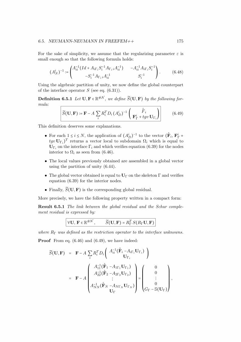
6.5. NEUMANN-NEUMANN IN FREEFEM++ 175
For the sake of simplicity, we assume that the regularizing parameter ε issmall enough so that the following formula holds:
(AiN)−1 ∶=⎛⎝A−1ii (Id +AiΓiS−1
i AΓi iA−1ii ) −A−1
ii AiΓiS−1i
−S−1i AΓi iA
−1ii S−1
i
⎞⎠. (6.48)
Using the algebraic partition of unity, we now define the global counterpartof the interface operator S (see eq. (6.31)).
Definition 6.5.1 Let U,F ∈ R#N , we define S(U,F) by the following for-mula:
S(U,F) ∶= F −A∑i
RTi Di (AiD)−1 (F i
FiΓ + tgvUΓi
) (6.49)
This definition deserves some explanations.
• For each 1 ≤ i ≤ N , the application of (AiD)−1 to the vector (Fi, Fi
Γ +tgvUΓi)T returns a vector local to subdomain Ωi which is equal toUΓi on the interface Γi and which verifies equation (6.39) for the nodesinterior to Ωi as seen from (6.46).
• The local values previously obtained are assembled in a global vectorusing the partition of unity (6.44).
• The global vector obtained is equal to UΓ on the skeleton Γ and verifiesequation (6.39) for the interior nodes.
• Finally, S(U,F) is the corresponding global residual.
More precisely, we have the following property written in a compact form:
Result 6.5.1 The link between the global residual and the Schur comple-ment residual is expressed by:
∀U, F ∈ R#N , S(U,F) = RTΓ S(RΓU,F)
where RΓ was defined as the restriction operator to the interface unknowns.
Proof From eq. (6.46) and (6.49), we have indeed:
S(U,F) = F −A∑i
RTi Di ( A−1ii (
Fi −AiΓiUΓi)
UΓi
)
= F −A
⎛⎜⎜⎜⎜⎜⎜⎜⎝
A−111(
F1 −A1Γ1UΓ1)
A−122(
F2 −A2Γ2UΓ2)
⋮A−1NN(
FN −ANΓNUΓN )
UΓ
⎞⎟⎟⎟⎟⎟⎟⎟⎠
=
⎛⎜⎜⎜⎜⎜⎜⎝
00⋮0
GΓ − S(UΓ)
⎞⎟⎟⎟⎟⎟⎟⎠
,
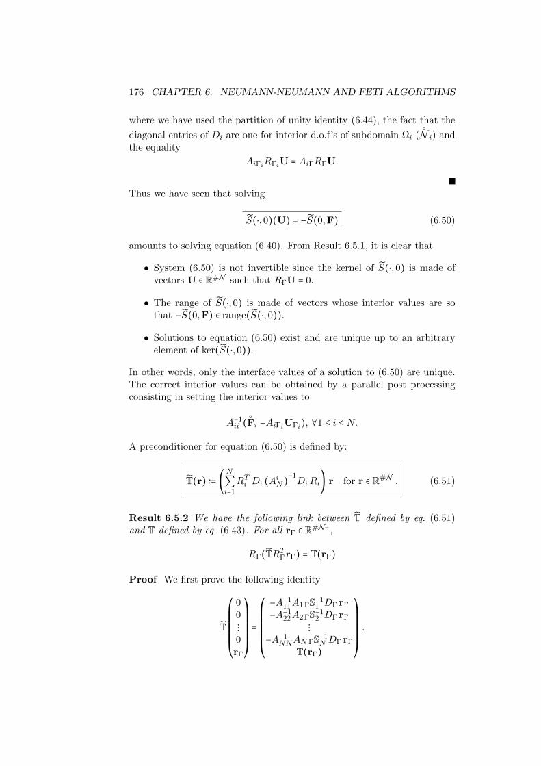
176 CHAPTER 6. NEUMANN-NEUMANN AND FETI ALGORITHMS
where we have used the partition of unity identity (6.44), the fact that the
diagonal entries of Di are one for interior d.o.f’s of subdomain Ωi (N i) and
the equality
AiΓiRΓiU = AiΓRΓU.
Thus we have seen that solving
S(⋅,0)(U) = −S(0,F) (6.50)
amounts to solving equation (6.40). From Result 6.5.1, it is clear that
• System (6.50) is not invertible since the kernel of S(⋅,0) is made ofvectors U ∈ R#N such that RΓU = 0.
• The range of S(⋅,0) is made of vectors whose interior values are sothat −S(0,F) ∈ range(S(⋅,0)).
• Solutions to equation (6.50) exist and are unique up to an arbitraryelement of ker(S(⋅,0)).
In other words, only the interface values of a solution to (6.50) are unique.The correct interior values can be obtained by a parallel post processingconsisting in setting the interior values to
A−1ii (
Fi −AiΓiUΓi), ∀1 ≤ i ≤ N.
A preconditioner for equation (6.50) is defined by:
T(r) ∶= (N
∑i=1
RTi Di (AiN)−1DiRi) r for r ∈ R#N . (6.51)
Result 6.5.2 We have the following link between T defined by eq. (6.51)and T defined by eq. (6.43). For all rΓ ∈ R#NΓ,
RΓ(TRTΓrΓ) = T(rΓ)
Proof We first prove the following identity
T
⎛⎜⎜⎜⎜⎜⎜⎝
00⋮0rΓ
⎞⎟⎟⎟⎟⎟⎟⎠
=
⎛⎜⎜⎜⎜⎜⎜⎝
−A−111A1 ΓS−1
1 DΓ rΓ
−A−122A2 ΓS−1
2 DΓ rΓ
⋮−A−1
NNAN ΓS−1N DΓ rΓ
T(rΓ)
⎞⎟⎟⎟⎟⎟⎟⎠
.
6.5. NEUMANN-NEUMANN IN FREEFEM++ 177
This shows that the action of T on the interface component of the residualamounts to that of T defined by formula (6.43). Then, for each subdomaini,1 ≤ i ≤ N , we have
(AiN)−1DiRi
⎛⎜⎜⎜⎜⎜⎜⎝
00⋮0rΓ
⎞⎟⎟⎟⎟⎟⎟⎠
= (AiN)−1 ( 0DΓirΓi
) = (−A−1ii AiΓ S−1
i DΓ rΓ
RΓi S−1i DΓ rΓ
) .
For the interior unknowns to the subdomains Di is the identity so that
Di(AiN)−1DiRi
⎛⎜⎜⎜⎜⎜⎜⎝
00⋮0rΓ
⎞⎟⎟⎟⎟⎟⎟⎠
= (−A−1ii AiΓ S−1
i DΓ rΓ
DΓiRΓi S−1i DΓ rΓ
) .
Finally, due to the fact that the global partition of unity (6.50) induces aninterface partition of unity , we have by left multiplying by RTi and summingover the subdomains:
T
⎛⎜⎜⎜⎜⎜⎜⎝
00⋮0rΓ
⎞⎟⎟⎟⎟⎟⎟⎠
=
⎛⎜⎜⎜⎜⎜⎜⎝
−A−111A1 ΓS−1
1 DΓ rΓ
−A−122A2 ΓS−1
2 DΓ rΓ
⋮−A−1
NNAN ΓS−1N DΓ rΓ
T(rΓ)
⎞⎟⎟⎟⎟⎟⎟⎠
.
To summarize,
• We solve the (ill-posed) linear system (6.50) by a conjugate gradientmethod preconditioned by operator T (6.51).
• The solution returned by the Krylov method is correct on the interfacebut interior values need to be corrected, see § 3.5 and the characteri-zation of the kernel and range of S(.,0) above.
• This correction is achieved by the following post processing step:
Ui= A−1
ii (Fi −AiΓiUΓi)
where UΓi is the restriction to Γi of the interface values UΓ.
6.5.1 FreeFem++ scripts
We are ready now to provide the FreeFem++ implementation. Thebeginning is identical of those of the Schwarz routines, except that the
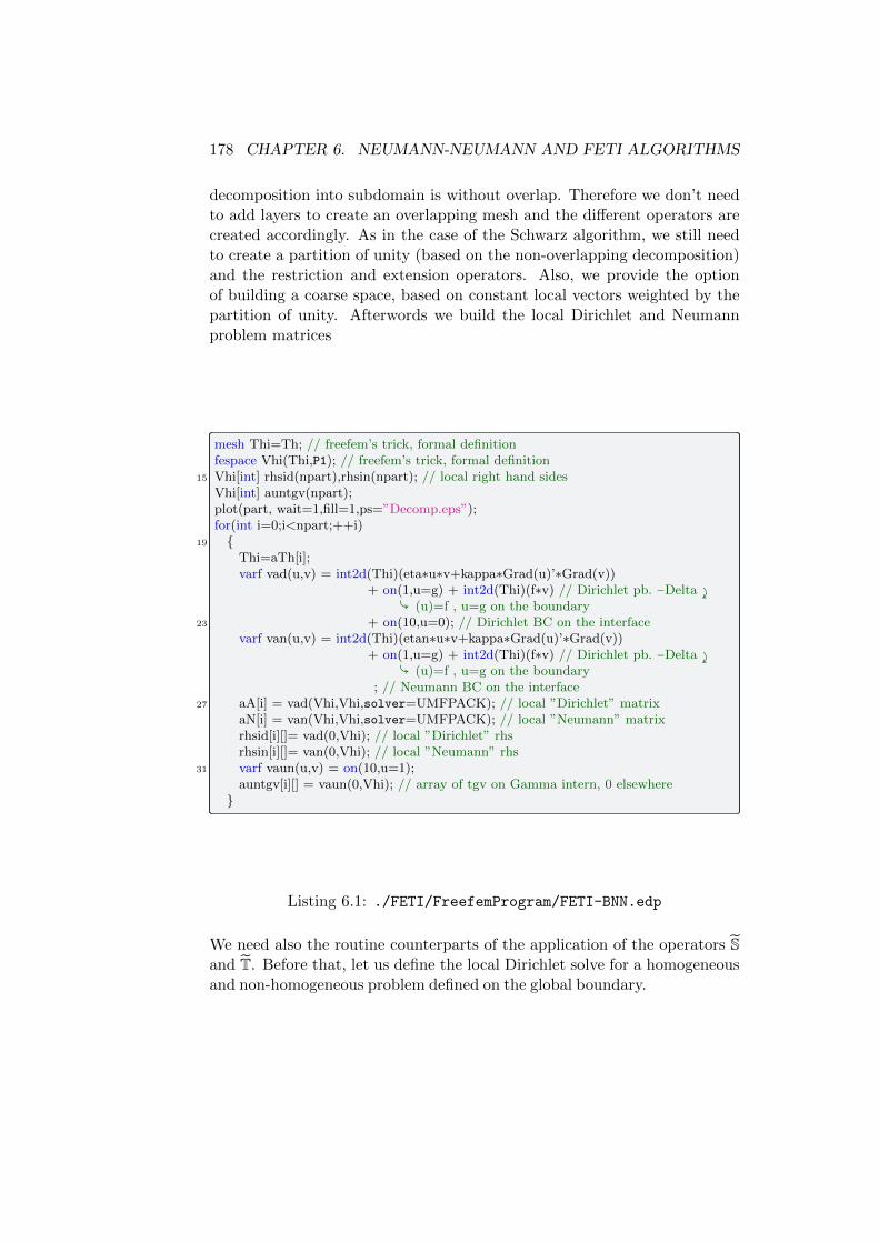
178 CHAPTER 6. NEUMANN-NEUMANN AND FETI ALGORITHMS
decomposition into subdomain is without overlap. Therefore we don’t needto add layers to create an overlapping mesh and the different operators arecreated accordingly. As in the case of the Schwarz algorithm, we still needto create a partition of unity (based on the non-overlapping decomposition)and the restriction and extension operators. Also, we provide the optionof building a coarse space, based on constant local vectors weighted by thepartition of unity. Afterwords we build the local Dirichlet and Neumannproblem matrices
mesh Thi=Th; // freefem’s trick, formal definitionfespace Vhi(Thi,P1); // freefem’s trick, formal definition
15 Vhi[int] rhsid(npart),rhsin(npart); // local right hand sidesVhi[int] auntgv(npart);plot(part, wait=1,fill=1,ps=”Decomp.eps”);for(int i=0;i<npart;++i)
19 Thi=aTh[i];varf vad(u,v) = int2d(Thi)(eta∗u∗v+kappa∗Grad(u)’∗Grad(v))
+ on(1,u=g) + int2d(Thi)(f∗v) // Dirichlet pb. −Delta ⤸Ç (u)=f , u=g on the boundary
23 + on(10,u=0); // Dirichlet BC on the interfacevarf van(u,v) = int2d(Thi)(etan∗u∗v+kappa∗Grad(u)’∗Grad(v))
+ on(1,u=g) + int2d(Thi)(f∗v) // Dirichlet pb. −Delta ⤸Ç (u)=f , u=g on the boundary
; // Neumann BC on the interface27 aA[i] = vad(Vhi,Vhi,solver=UMFPACK); // local ”Dirichlet” matrix
aN[i] = van(Vhi,Vhi,solver=UMFPACK); // local ”Neumann” matrixrhsid[i][]= vad(0,Vhi); // local ”Dirichlet” rhsrhsin[i][]= van(0,Vhi); // local ”Neumann” rhs
31 varf vaun(u,v) = on(10,u=1);auntgv[i][] = vaun(0,Vhi); // array of tgv on Gamma intern, 0 elsewhere
Listing 6.1: ./FETI/FreefemProgram/FETI-BNN.edp
We need also the routine counterparts of the application of the operators Sand T. Before that, let us define the local Dirichlet solve for a homogeneousand non-homogeneous problem defined on the global boundary.

6.5. NEUMANN-NEUMANN IN FREEFEM++ 179
func real[int] extendDir(real[int] ud, bool hom)3 // Solve local Dirichlet problems with ud at the interface
// homogeneous on the real boundary (hom = 1) or not (hom = 0)
Vh s=0;7 for(int i=0;i<npart;++i)
real[int] ui = Rih[i]∗ud; // local solutionreal[int] bi = ui .∗ auntgv[i][]; // take into account the interface conditions
11 if (hom)bi = auntgv[i][] ? bi : 0; // update rhs
elsebi = auntgv[i][] ? bi : rhsid[i][];
15 ui= aA[i] −1∗ bi; // solve local Dirichlet problembi = Dih[i]∗ui; // use the partition of unitys[]+= Rih[i]’∗bi; // extend the local solution globally
19 return s[];
Listing 6.2: ./FreefemCommon/matvecDtNtD.idp
The effect of operator S is given by
func real[int] A(real[int] &l) // DtN operator
26 Vh ui, rn, s;ui[]=l.∗intern[];s[] = extendDir(ui[],1);rn[]= Aglobal∗s[];
30 rn[] = rn[] .∗ intern[];return rn[];
Listing 6.3: ./FreefemCommon/matvecDtNtD.idp
and that of operator T is given by
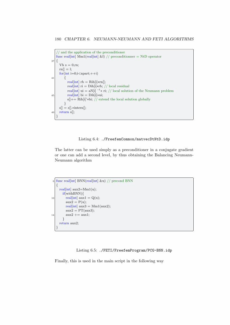
180 CHAPTER 6. NEUMANN-NEUMANN AND FETI ALGORITHMS
// and the application of the preconditionerfunc real[int] Mm1(real[int] &l) // preconditionner = NtD operator
37 Vh s = 0,rn;rn[] = l;for(int i=0;i<npart;++i)
41 real[int] rb = Rih[i]∗rn[];real[int] ri = Dih[i]∗rb; // local residual
real[int] ui = aN[i] −1∗ ri; // local solution of the Neumann problem45 real[int] bi = Dih[i]∗ui;
s[]+= Rih[i]’∗bi; // extend the local solution globally
s[] = s[].∗intern[];49 return s[];
Listing 6.4: ./FreefemCommon/matvecDtNtD.idp
The latter can be used simply as a preconditioner in a conjugate gradientor one can add a second level, by thus obtaining the Balancing Neumann-Neumann algorithm
6 func real[int] BNN(real[int] &u) // precond BNN
real[int] aux2=Mm1(u);if(withBNN)
10 real[int] aux1 = Q(u);aux2 = P(u);real[int] aux3 = Mm1(aux2);aux2 = PT(aux3);
14 aux2 += aux1;
return aux2;
Listing 6.5: ./FETI/FreefemProgram/PCG-BNN.idp
Finally, this is used in the main script in the following way

6.5. NEUMANN-NEUMANN IN FREEFEM++ 181
0 20 40 60 80 100 120 14010−9
10−8
10−7
10−6
10−5
10−4
10−3
10−2
10−1
100Comparison of convergence Neumann−Neumann
Iterations
Res
idua
l
4x48x810x10
0 1 2 3 4 5 6 710−8
10−7
10−6
10−5
10−4
10−3
10−2
10−1
100Comparison of convergence Balancing Neumann−Neumann
Iterations
Res
idua
l
4x48x810x10
Figure 6.7: Neumann-Neumann convergence without (left) and with (right)coarse space for a uniform decomposition
Vh s, b, un, gd;37 include ”../../FreefemCommon/matvecDtNtd.idp”
include ”../../FreefemCommon/coarsespace.idp”// compute rhs of the interface problem: b[]un = 0;
41 gd[]=g;un[]+= bord[].∗gd[];s[] = extendDir(un[],0);b[]= Aglobal∗s[];
45 b[]−= rhsglobal[];b[] ∗= −1;include ”PCG−BNN.idp”Vh lam = 0,sol;
49 lam[] = lam[].∗intern[]; // insures that the first iterate verifieslam[]+= bord[].∗gd[]; // the global BC, from iter=1 on this is truesol[] = myPCG(lam[],tol,maxit);sol[] = extendDir(sol[],0);
53 Vh err = sol−uglob;plot(sol,cmm=” Final Solution”, wait=1,dim=3,fill=1,value=1);cout << ” Final error: ” << err[].linfty << endl;
Listing 6.6: ./FETI/FreefemProgram/FETI-BNN.edp
In Figures 6.7 and 6.8, we report results for uniform and Metis decomposi-tions into 4×4, 8×8 and 10×10 subdomains. We use the Neumann-Neumannmethod as a preconditioner in a Krylov method. In the first set of tests themethod is used without a coarse space and we see that the iteration num-ber depends linearly on the total number of domains and not only on thenumber of domains in one direction as in the case of the Schwarz methods.By adding a coarse space, the behavior becomes insensitive to the numberof subdomains as expected. Note that the convergence is better in the caseof uniform decompositions than in the case of decompositions using Metis.
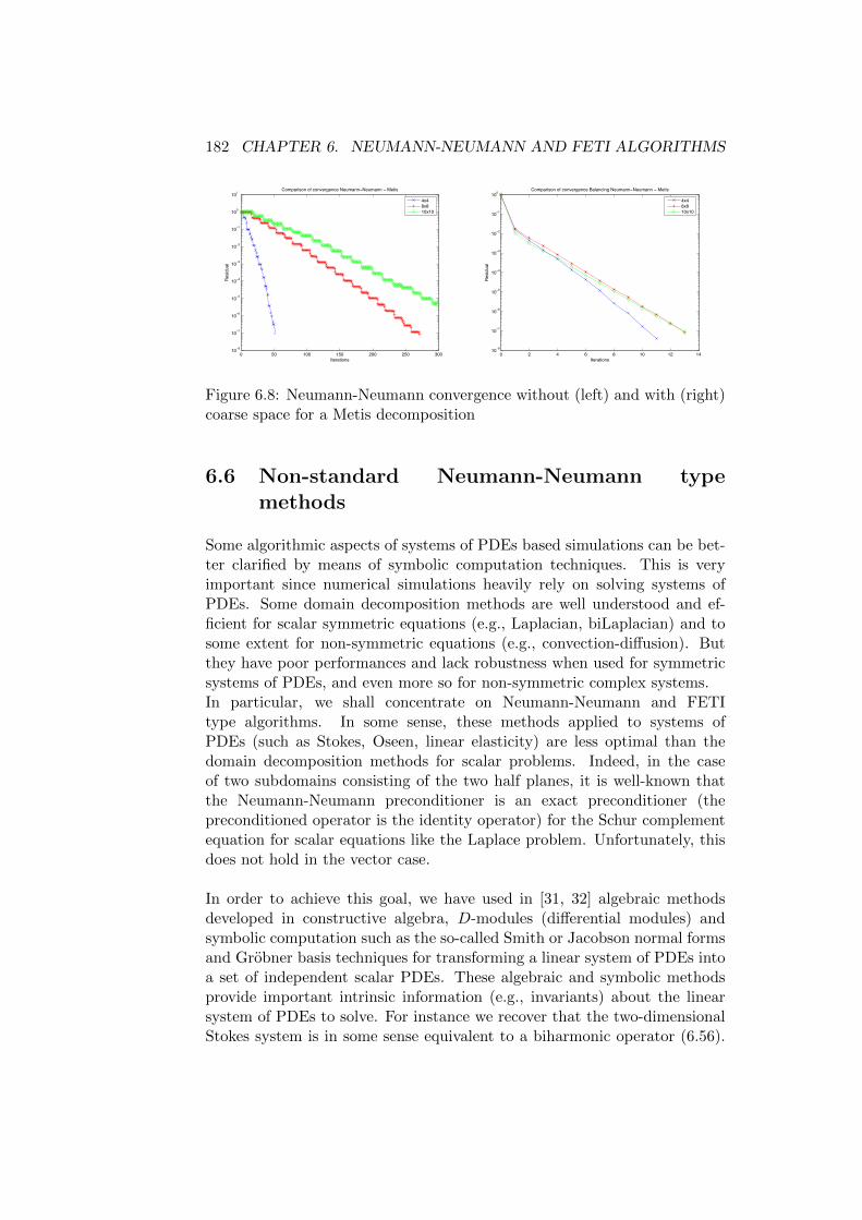
182 CHAPTER 6. NEUMANN-NEUMANN AND FETI ALGORITHMS
0 50 100 150 200 250 30010−8
10−7
10−6
10−5
10−4
10−3
10−2
10−1
100
101Comparison of convergence Neumann−Neumann − Metis
Iterations
Res
idua
l
4x48x810x10
0 2 4 6 8 10 12 1410−8
10−7
10−6
10−5
10−4
10−3
10−2
10−1
100Comparison of convergence Balancing Neumann−Neumann − Metis
Iterations
Res
idua
l
4x48x810x10
Figure 6.8: Neumann-Neumann convergence without (left) and with (right)coarse space for a Metis decomposition
6.6 Non-standard Neumann-Neumann typemethods
Some algorithmic aspects of systems of PDEs based simulations can be bet-ter clarified by means of symbolic computation techniques. This is veryimportant since numerical simulations heavily rely on solving systems ofPDEs. Some domain decomposition methods are well understood and ef-ficient for scalar symmetric equations (e.g., Laplacian, biLaplacian) and tosome extent for non-symmetric equations (e.g., convection-diffusion). Butthey have poor performances and lack robustness when used for symmetricsystems of PDEs, and even more so for non-symmetric complex systems.In particular, we shall concentrate on Neumann-Neumann and FETItype algorithms. In some sense, these methods applied to systems ofPDEs (such as Stokes, Oseen, linear elasticity) are less optimal than thedomain decomposition methods for scalar problems. Indeed, in the caseof two subdomains consisting of the two half planes, it is well-known thatthe Neumann-Neumann preconditioner is an exact preconditioner (thepreconditioned operator is the identity operator) for the Schur complementequation for scalar equations like the Laplace problem. Unfortunately, thisdoes not hold in the vector case.
In order to achieve this goal, we have used in [31, 32] algebraic methodsdeveloped in constructive algebra, D-modules (differential modules) andsymbolic computation such as the so-called Smith or Jacobson normal formsand Grobner basis techniques for transforming a linear system of PDEs intoa set of independent scalar PDEs. These algebraic and symbolic methodsprovide important intrinsic information (e.g., invariants) about the linearsystem of PDEs to solve. For instance we recover that the two-dimensionalStokes system is in some sense equivalent to a biharmonic operator (6.56).

6.6. NON-STANDARD NEUMANN-NEUMANN TYPE METHODS 183
In fluid mechanics, it relates to the stream function formulation [11]. Thesebuild-in properties need to be taken into account in the design of newnumerical methods, which can supersede the usual ones based on a directextension of the classical scalar methods to linear systems of PDEs. Bymeans of these techniques, it is also possible to transform the linear systemof PDEs into a set of decoupled PDEs under certain types of invertibletransformations. One of these techniques is the so-called Smith normalform of the matrix of OD operators associated with the linear system.The Smith normal form has already been successfully applied to openproblems in the design of Perfectly Matched Layers (PML). The theory ofPML for scalar equations was well-developed and the usage of the Smithnormal form allowed to extend these works to systems of PDEs. In [142],a general approach is proposed and applied to the particular case of thecompressible Euler equations that model aero-acoustic phenomena and in[10] for shallow-water equations.
For domain decomposition methods, several results have been obtained oncompressible Euler equations [59, 60], Stokes and Oseen systems [61, 62]or in [101] where a new method in the ”Smith” spirit has been derived.Previously the computations were performed heuristically, whereas in [31,32], a systematic way to build optimal algorithms for given PDE systemswas shown.
Notations. If R is a ring, then Rp×q is the set of p×q matrices with entries inR and GLp(R) is the group of invertible matrices of Rp×p, namely GLp(R) ∶=E ∈ Rp×p ∣ ∃ F ∈ Rp×p ∶ EF = F E = Ip. An element of GLp(R) is called anunimodular matrix. A diagonal matrix with elements di’s will be denoted bydiag(d1, . . . , dp). If k is a field (e.g., k = Q, R, C), then k[x1, . . . , xn] is thecommutative ring of polynomials in x1, . . . , xn with coefficients in k. In whatfollows, k(x1, . . . , xn) will denote the field of rational functions in x1, . . . , xnwith coefficients in k. Finally, if r, r′ ∈ R, then r′ ∣ r means that r′ divides r,i.e., there exists r′′ ∈ R such that r = r′′ r′.
6.6.1 Smith normal form of linear systems of PDEs
We first introduce the concept of Smith normal form [176] of a matrix withpolynomial entries (see, e.g., [94] or [188], Theorem 1.4). The Smith nor-mal form is a mathematical technique which is classically used in moduletheory, linear algebra, symbolic computation, ordinary differential systems,and control theory. It was first developed to study matrices with integerentries.
Theorem 6.6.1 Let k be a field, R = k[s], p a positive integer and A ∈ Rp×p.

184 CHAPTER 6. NEUMANN-NEUMANN AND FETI ALGORITHMS
Then, there exist two matrices E ∈ GLp(R) and F ∈ GLp(R) such that
A = E S F,
where S = diag(d1, . . . , dp) and the di ∈ R satisfying d1 ∣d2 ∣⋯ ∣dp. In partic-ular, we can take di =mi/mi−1, where mi is the greatest common divisor ofall the i× i-minors of A (i.e., the determinants of all i× i-submatrices of A),with the convention that m0 = 1. The matrix S = diag(d1, . . . , dp) ∈ Rp×p iscalled a Smith normal form of A.
We note that E ∈ GLp(R) is equivalent to det(E) is an invertible polyno-mial, i.e., det(E) ∈ k ∖ 0. Also, in what follows, we shall assume that thedi’s are monic polynomials, i.e., their leading coefficients are 1, which willallow us to call the matrix S = diag(d1, . . . , dp) the Smith normal form of A.But, the unimodular matrices E and F are not uniquely defined by A. Theproof of Theorem 6.6.1 is constructive and gives an algorithm for computingmatrices E, S and F . The computation of Smith normal forms is availablein many computer algebra systems such as Maple, Mathematica, Magma. . .
Consider now the following model problem in Rd with d = 2,3:
Ld(w) = g in Rd, ∣w(x)∣→ 0 for ∣x∣→∞. (6.52)
For instance, Ld(w) can represent the Stokes/Oseen/linear elasticity opera-tors in dimension d. In the case of the Oseen equation, the diagonal matrixS (6.57) is the product of a Laplace operator and a convection-diffusion op-erator. We suppose that the inhomogeneous linear system of PDEs (6.52)has constant coefficients, then it can be rewritten as
Adw = g, (6.53)
where Ad ∈ Rp×p, R = k[∂x, ∂y] (resp., R = k[∂x, ∂y, ∂z]) for d = 2 (resp.,d = 3) and k is a field.In what follows, we shall study the domain decomposition problem in whichRd is divided into two half planes subdomains. We assume that the directionnormal to the interface of the subdomains is particularized and denoted by∂x. If Rx = k(∂y)[∂x] for d = 2 or Rx = k(∂y, ∂z)[∂x] for d = 3, then,computing the Smith normal form of the matrix Ad ∈ Rp×px , we obtain Ad =E S F , where S ∈ Rp×px is a diagonal matrix, E ∈ GLp(Rx) and F ∈ GLp(Rx).The entries of the matrices E, S, F are polynomials in ∂x, and E andF are unimodular matrices, i.e., det(E), det(F ) ∈ k(∂y) ∖ 0 if d = 2, ordet(E), det(F ) ∈ k(∂y, ∂z)∖ 0 if d = 3. We recall that the matrices E andF are not unique contrary to S. Using the Smith normal form of Ad, weget:
Adw = g ⇔ ws ∶= F w, Sws = E−1 g. (6.54)
6.6. NON-STANDARD NEUMANN-NEUMANN TYPE METHODS 185
In other words, (6.54) is equivalent to the uncoupled linear system:
Sws = E−1 g. (6.55)
Since E ∈ GLp(Rx) and F ∈ GLp(Rx), the entries of their inverses are stillpolynomial in ∂x. Thus, applying E−1 to the right-hand side g of Adw = gamounts to taking k-linear combinations of derivatives of g with respect tox. If Rd is split into two subdomains R− × Rd−1 and R+ × Rd−1, then theapplication of E−1 and F−1 to a vector can be done for each subdomainindependently. No communication between the subdomains is necessary.In conclusion, it is enough to find a domain decomposition algorithm forthe uncoupled system (6.55) and then transform it back to the original one(6.53) by means of the invertible matrix F over Rx. This technique can beapplied to any linear system of PDEs once it is rewritten in a polynomialform. The uncoupled system acts on the new dependent variables ws, whichwe shall further call Smith variables since they are issued from the Smithnormal form.
Remark 6.6.1 Since the matrix F is used to transform (6.55) to (6.53)(see the first equation of the right-hand side of (6.54)) and F is not unique,we need to find a matrix F as simple as possible (e.g., F has minimal degreein ∂x) so that to obtain a final algorithm whose form can be used for practicalcomputations.
Example 6.6.1 Consider the two dimensional elasticity operator definedby E2(u) ∶= −µ∆u − (λ + µ)∇divu. If we consider the commutative poly-nomial rings R = Q(λ,µ)[∂x, ∂y], Rx = Q(λ,µ)(∂y)[∂x] = Q(λ,µ, ∂y)[∂x]and
A2 = ((λ + 2µ)∂2
x + µ∂2y (λ + µ)∂x ∂y
(λ + µ)∂x ∂y µ∂2x + (λ + 2µ)∂2
y
) ∈ R2×2
the matrix of PD operators associated with E2, i.e., E2(u) = A2 u, then theSmith normal form of A2 ∈ R2×2
x is defined by:
SA2 = (1 0
0 ∆2 ) . (6.56)
The particular form of SA2 shows that, over Rx, the system of PDEs for thelinear elasticity in R2 is algebraically equivalent to a bi-harmonic equation.
Example 6.6.2 Consider the two dimensional Oseen operator O2(w) =O2(v, q) ∶= (cv−ν∆v+b ⋅∇v+∇q,∇⋅v), where b is the convection velocity.If b = 0, then we obtain the Stokes operator S2(w) = S2(v, q) ∶= (cv −ν∆v + ∇q,∇ ⋅ v). If R = Q(b1, b2, c, ν)[∂x, ∂y], Rx = Q(b1, b2, c, ν)(∂y)[∂x] =

186 CHAPTER 6. NEUMANN-NEUMANN AND FETI ALGORITHMS
Q(b1, b2, c, ν, ∂y)[∂x] and
O2 =⎛⎜⎜⎝
−ν (∂2x + ∂2
y) + b1 ∂x + b2 ∂y + c 0 ∂x
0 −ν (∂2x + ∂2
y) + b1 ∂x + b2 ∂y + c ∂y
∂x ∂y 0
⎞⎟⎟⎠
the matrix of PD operators associated with O2, i.e., O2(w) = O2 w, thenthe Smith normal form of O2 ∈ R3×3
x is defined by:
SO2 =⎛⎜⎜⎝
1 0 0
0 1 0
0 0 ∆L2
⎞⎟⎟⎠, L2 = c − ν∆ + b ⋅ ∇. (6.57)
From the form of SO2 we can deduce that the two-dimensional Oseen equa-tions can be mainly characterized by the scalar fourth order PD operator∆L2. This is not surprising since the stream function formulation of theOseen equations for d = 2 gives the same PDE for the stream function.
Remark 6.6.2 The above applications of Smith normal forms suggest thatone should design an optimal domain decomposition method for the bi-harmonic operator ∆2 (resp., L2 ∆) in the case of linear elasticity (resp., theOseen/Stokes equations) for the two-dimensional problems, and then trans-form it back to the original system.
6.6.2 An optimal algorithm for the bi-harmonic operator
We give here an example of Neumann-Neumann methods in its iterativeversion for Laplace and biLaplace equations. For simplicity, consider a de-composition of the domain Ω = R2 into two half planes Ω1 = R− × R andΩ2 = R+ ×R. Let the interface 0×R be denoted by Γ and (ni)i=1,2 be theoutward normal of (Ωi)i=1,2.We consider the following problem:
−∆u = f in R2,∣u(x)∣ → 0 for ∣ x∣→∞. (6.58)
and the following Neumann-Neumann algorithm applied to (6.58):
This algorithm is optimal in the sense that it converges in two iterations.
Since the bi-harmonic operator seems to play a key role in the design of anew algorithm for both Stokes and elasticity problem in two dimensions, weneed to build an optimal algorithm for it. We consider the following problem:
Find φ ∶ R2 → R such that∆2φ = g in R2, ∣φ(x)∣→ 0 for ∣x∣→∞. (6.60)
6.6. NON-STANDARD NEUMANN-NEUMANN TYPE METHODS 187
Let unΓ be the interface solution at iteration n. We obtain un+1Γ from unΓ by
the following iterative procedure
−∆ui,n = f, in Ωi,
ui,n = unΓ, on Γ,
⎧⎪⎪⎪⎪⎨⎪⎪⎪⎪⎩
−∆ui,n = 0, in Ωi,
∂ui,n
∂ni= −1
2(∂u
1,n
∂n1+ ∂u
2,n
∂n2) , on Γ,
(6.59)and then un+1
Γ = unΓ + 12(u1,n + u2,n).
Let (φnΓ,DφnΓ) be the interface solution at iteration n (suppose also thatφ0
Γ = φ0∣Γ, Dφ0Γ = (∆φ0)Γ). We obtain (φn+1
Γ ,DφnΓ) from (φnΓ,DφnΓ) by thefollowing iterative procedure
⎧⎪⎪⎪⎪⎨⎪⎪⎪⎪⎩
−∆2φi,n = f, in Ωi,
φi,n = φnΓ, on Γ,
∆φi,n = DφnΓ, on Γ,
⎧⎪⎪⎪⎪⎪⎪⎪⎪⎪⎪⎨⎪⎪⎪⎪⎪⎪⎪⎪⎪⎪⎩
−∆2φi,n = 0, in Ωi,
∂φi,n
∂ni= −1
2(∂φ
1,n
∂n1+ ∂φ
2,n
∂n2) , on Γ,
∂∆φi,n
∂ni= −1
2(∂∆φ1,n
∂n1+ ∂∆φ2,n
∂n2) , on Γ,
(6.61)and then φn+1
Γ = φnΓ + 12(φ1,n + φ2,n) , Dφn+1
Γ =DφnΓ + 12(∆φ1,n + ∆φ2,n).
and the following “Neumann-Neumann” algorithm applied to (6.60):This is a generalization of the Neumann-Neumann algorithm for the ∆operator and is also optimal (the proof can be found in [61]).
Now, in the case of the two dimensional linear elasticity, φ represents the sec-ond component of the vector of Smith variables, that is, φ = (ws)2 = (Fu)2,where u = (u, v) is the displacement field. Hence, we need to replace φwith (Fu)2 into the algorithm for the biLaplacian, and then simplify itusing algebraically admissible operations. Thus, one can obtain an optimalalgorithm for the Stokes equations or linear elasticity depending on theform of F . From here comes the necessity of choosing in a proper way thematrix F (which is not unique), used to define the Smith normal form,in order to obtain a “good” algorithm for the systems of PDEs from theoptimal one applied to the bi-harmonic operator. In [59] and [61], thecomputation of the Smith normal forms for the Euler equations and theStokes equations was done by hand or using the Maple command Smith.Surprisingly, the corresponding matrices F have provided good algorithmsfor the Euler equations and the Stokes equations even if the approach wasentirely heuristic.
The efficiency of our algorithms heavily relies on the simplicity of the Smith
188 CHAPTER 6. NEUMANN-NEUMANN AND FETI ALGORITHMS
variables, that is on the entries of the unimodular matrix F used to com-pute the Smith normal form of the matrix A. Within a constructive algebraicanalysis approach, we developed a method for constructing many possibleSmith variables (completion problem). Taking into account physical aspects,the user can then choose the simplest one among them. Also, in the algo-rithms presented in the previous sections, we have equations in the domainsΩi and interface conditions on Γ obtained heuristically. We have designedan automatic way to reduce the interface conditions with respect to theequations in the domains (reduction problem). For more details and explicitcomputations, we refer the reader to [31, 32].
6.6.3 Some optimal algorithms
After performing the completion and the reduction of the interface condi-tions, we can give examples of optimal algorithms.
Example 6.6.3 Consider the elasticity operator:
Ed u = − div σ (u), σ(u) = µ (∇u + (∇u)T ) + λ div u Id.
If d = 2, then the completion algorithm gives two possible choices for F :
F =⎛⎝−∂x (µ∂2
x−λ∂2y)
(λ+µ)∂3y
1
1 0
⎞⎠, F =
⎛⎝
1 − (λ+µ)∂x ((3µ+2λ)∂2y+(2µ+λ)∂
2x)
∂3y
0 1
⎞⎠.
(6.62)By replacing φ into the Neumann-Neumann algorithm for the biLaplacianby (Fu)2 and re-writing the interface conditions, using the equations insidethe domain like in [61], we get two different algorithms for the elasticitysystem. Note that, in the first case of (6.62), φ = u, and, in the second one,φ = v (where u = (u, v)). Below, we shall write in detail the algorithm inthe second case. To simplify the writing, we denote by uτ = u ⋅ τ , un = u ⋅n,σnn(u) = (σ(u) ⋅ n) ⋅ n, σnτ(u) = (σ(u) ⋅ n) ⋅ τ .
Remark 6.6.3 We found an algorithm with a mechanical meaning: Findthe tangential part of the normal stress and the normal displacement at theinterface so that the normal part of the normal stress and the tangentialdisplacement on the interface match. This is very similar to the originalNeumann-Neumann algorithm, which means that the implementation effortof the new algorithm from an existing Neumann-Neumann is negligible (thesame type of quantities − displacement fields and efforts − are imposed atthe interfaces), except that the new algorithm requires the knowledge of somegeometric quantities, such as normal and tangential vectors. Note also that,with the adjustment of the definition of tangential quantities for d = 3, thealgorithm is the same, and is also similar to the results in [61].

6.6. NON-STANDARD NEUMANN-NEUMANN TYPE METHODS 189
Let (unΓ, σnΓ) be the interface solution at iteration n (suppose also thatu0
Γ = (u0τ)∣Γ, σ0
Γ = (σsnn(u0))∣Γ). We obtain (un+1Γ , σnΓ) from (unΓ, σnΓ) by
the following iterative procedure
⎧⎪⎪⎪⎪⎨⎪⎪⎪⎪⎩
E2(ui,n) = f, in Ωi,
u1,nτi = unΓ, on Γ,
σnini(ui,n) = σnΓ, on Γ,
⎧⎪⎪⎪⎪⎪⎪⎪⎪⎪⎪⎨⎪⎪⎪⎪⎪⎪⎪⎪⎪⎪⎩
E2(ui,n) = 0, in Ωi,
ui,nτi = −1
2(u1,n
n1+ u2,n
n2) , on Γ,
σniτi(ui,n) = −1
2(σn1τ1(u1,n) + σn2τ2(u2,n)) ,
on Γ,(6.63)
and un+1Γ = unΓ + 1
2(u1,n
τ1 + u2,nτ2 ) , σn+1
Γ = σnΓ + 12(σn1n1(u1,n) + σn2n2(u2,n)).
All algorithms and interface conditions are derived for problems posed onthe whole space, since for the time being, this is the only way to treat fromthe algebraic point of view these problems. The effect of the boundarycondition on bounded domains cannot be quantified with the same tools.All the algorithms are designed in the PDE level and it is very importantto choose the right discrete framework in order to preserve the optimalproperties. For example, in the case of linear elasticity a good candidatewould be the TDNNS finite elements that can be found in [157] and thealgorithms obtained by these algebraic techniques have been used to designa FETI-TDNNS method [156].

190 CHAPTER 6. NEUMANN-NEUMANN AND FETI ALGORITHMS
Chapter 7
Robust Coarse Spaces viaGeneralized Eigenproblems:the GenEO method
We have already analyzed in Chapter 5 two-level additive Schwarz methodsfor a Poisson problem with a coarse space motivated by heuristic ideas.The condition number estimates were based on a specific tool to domaindecomposition methods and multigrid methods namely the notion of stabledecomposition (definition 5.4.1) as well as on functional analysis resultssuch as Poincare inequalities or trace theorems and on a numerical analysisinterpolation inequality (5.8). In this chapter, we present the GenEO(Generalized Eigenvalue in the Overlap) method to build coarse spaces forwhich any targeted convergence rate can be achieved. The constructionis as algebraic as possible. We shall make a heavy use of a generalizationof the stable decomposition notion, namely the Fictitious Space Lemma,see § 7.2.1. This abstract result is based on writing domain decompositionmethods as a product of three linear operators.
As we also mentioned previously, the main motivation to build a robustcoarse space for a two-level additive Schwarz method is to achieve scalabilitywhen solving highly heterogeneous problems i.e. for which the convergenceproperties do not depend on the variation of the coefficient. Recently, forscalar elliptic problems, operator dependent coarse spaces have been built inthe case where coefficients are not resolved by the subdomain partition, seee.g. [63, 70, 84, 83, 102, 148, 160, 172, 173]. We have seen in Chapter 5 thata very useful tool for building coarse spaces for which the correspondingtwo-level method is robust, regardless of the partition into subdomains andof the coefficient distribution, is the solution of local generalized eigenvalueproblems. In this spirit, for the Darcy problem, [84] proposes to solve localgeneralized eigenvalue problems on overlapping coarse patches and local
191

192 CHAPTER 7. GENEO COARSE SPACE
contributions are then ’glued together’ via a partition of unity to obtain aglobal coarse space. More recently [83, 70] and [148, 63] have built on theseideas and proposed different coarse spaces based on different generalizedeigenvalue problems. The theoretical results in [63] rely on uniform (in thecoefficients) weighted Poincare inequalities and they have two drawbacks:(i) at the theoretical level some assumptions are needed on the coefficientdistribution in the overlaps and (ii) the arguments cannot be generalizedeasily to the case of systems of PDEs because the maximum principle doesnot hold anymore.
As a remedy to these drawbacks, in [178], we proposed a coarse spaceconstruction based on Generalized Eigenproblems in the Overlap (whichwe will refer to as the GenEO coarse space); the method was previouslyintroduced in [177] by the same authors. This particular construction hasbeen applied successfully to positive definite systems of PDEs discretized byfinite elements with only a few extra assumptions. The resulting generalizedeigenvalue problems are closely related, but different to the ones proposedin [70]. Which of the two approaches is better in practice in terms ofstability versus coarse space size is still the object of ongoing research, seefor example [186].
In this chapter, the GenEO method, as well as most classical two-level meth-ods are presented in a different light, under a common framework. Moreover,their convergence can be proven in an abstract setting, provided that theassumptions of the Fictitious Space Lemma are satisfied. Before stating thisLemma, we first reformulate the two-level ASM method in this framework.
7.1 Reformulation of the Additive SchwarzMethod
In this section we make a first step in the use of the abstract theory ofthe “Fictitious Space Lemma” 7.2.2 by better formalizing the AdditiveSchwarz Method (ASM). In order to simplify the presentation, we will placeourselves directly in an algebraic setting where the set of degrees of freedomN is decomposed into N subsets (Ni)1≤i≤N . In this framework we also havea partition of unity
N
∑i=1
RTi DiRi = Id
as defined in paragraph 1.3 equation (1.25). The coarse space is of size #N0
and spanned by the columns of a rectangular matrix RT0 of size #N ×#N0.Note that most of the assumptions of this lemma are verified without theprecise definition of a coarse space. That is why, the latter will be specifiedlater on in Definition 7.4.2 only when the stable decomposition property

7.1. REFORMULATION OF THE ADDITIVE SCHWARZ METHOD193
requires it.
In the fictitious space lemma (see Lemma 7.2.2) a certain number of abstractingredients are needed. These ingredients can be easily identified in the caseof the ASM. This intuitive introduction will give the general flavour of themethods exposed later on. We will come to the abstract framework afterthis short presentation.
Definition 7.1.1 (ASM components in the Fictitious Space Lemma)Two Hilbert spaces H, HD, two other associated bilinear forms and inducedscalar products as well as the RASM,2 operator between them are defined asfollows.
• Space H ∶= R#N endowed with the standard Euclidian scalar product.We consider another bilinear form a defined by :
a ∶H ×H → R, (U,V)z→ a(U,V) ∶= VTAU. (7.1)
where A is the matrix of the problem we want to solve. Recall thatmatrix A is symmetric positive definite.
• Space HD, defined as the product space
HD ∶= R#N0 ×N
∏i=1
R#Ni (7.2)
is endowed with standard scalar Euclidian product. For U = (Ui)0≤i≤N ,V = (Vi)0≤i≤N with Ui,Vi ∈ R#Ni, the bilinear form b is defined by
b ∶HD ×HD Ð→ R
(U ,V) z→ b(U ,V) ∶=N
∑i=0
a(RTi Ui,RTi Vi) =
N
∑i=0
VTi (RiARTi )Ui
∶= VTBU ,(7.3)
where B ∶HD →HD is the operator defined by
∀ U = (Ui)0≤i≤N ∈HD B(U) ∶= (RiARTi Ui)0≤i≤N . (7.4)
Note that B is actually a block diagonal operator whose inverse is:
∀ U = (Ui)0≤i≤N ∈HD B−1(U) ∶= ((RiARTi )−1Ui)0≤i≤N .
• The linear operator RASM,2 is defined as:
RASM,2 ∶HD Ð→H, (Ui)0≤i≤N ↦N
∑i=0
RTi Ui. (7.5)
194 CHAPTER 7. GENEO COARSE SPACE
After having settled these ingredients, we can proceed to the reformulationof the Additive Schwarz Method.
Lemma 7.1.1 (ASM in terms of Fictitious Space Lemma) Thetwo-level ASM preconditioner
M−1ASM,2 =
N
∑i=0
RTi (RiARTi )−1Ri (7.6)
can be re-written as
M−1ASM,2 =RASM,2B
−1R∗ASM,2 , (7.7)
where the operator R∗ASM,2 ∶H →HD is the adjoint of the operator RASM,2
with respect to the standard Euclidean scalar products and operator B isdefined in (7.4).
Proof First of all, note that by definition R∗ASM,2 can be written as:
(R∗ASM,2(U),V)2 ∶= (U,RASM,2(V))2, ∀U ∈H, V ∶= (Vi)0≤i≤N ∈HD.
or in other words:
N
∑i=0
VTi (R∗
ASM,2(U))i ∶= UTRASM,2(V) ,
that isN
∑i=0
VTi (R∗
ASM,2(U))i ∶= UTN
∑i=0
RTi Vi =N
∑i=0
VTi RiU .
Since this equality is valid for arbitrary Vi, we have the identification:
R∗ASM,2(U) = (RiU)0≤i≤N . (7.8)
which leads to the re-writing (7.7) of the Additive Schwarz Method.The explanation of the application of the preconditionner in term of theseoperators is the following
• According to (7.8), the right most operator R∗ASM,2 decomposes a
global vector in H into local components in HD
• The middle operator B−1 corresponds to solving a coarse problem andN local Dirichlet problems
• RASM,2 interpolates the modified local components into a global vectorin H.
As we shall see in the sequel of the chapter, this abstract form is also validfor many domain decomposition methods such as the balancing Neumann-Neumann preconditioner (BNN) and a modified version of the OptimizedSchwarz method (OSM). It will enable us to both analyze their conditionnumber and propose new coarse space constructions.

7.2. MATHEMATICAL FOUNDATION 195
7.2 Mathematical Foundation
In this paragraph we present a few abstract lemmas that are needed inthe sequel. Lemmas 7.2.2 and 7.2.7 are at the core of the study of manymultilevel methods. Lemma 7.2.5 is specific to the GenEO method we willintroduce.
7.2.1 Fictitious Space Lemma
We first state the lemma proved in [150, 149] as it is written in [105]. In itsproof we need the following auxiliary result:
Lemma 7.2.1 (Auxiliary result) Let m be an integer, A1,A2 ∈ Rm×m betwo symmetric positive definite matrices. Suppose there exists a constant csuch that
(A1u,u) ≤ c (A2u,u), ∀u ∈ Rm .Then, A−1
2 A1 has real eigenvalues that are bounded by constant c.
Lemma 7.2.2 (Fictitious Space Lemma) Let H and HD be two Hilbertspaces, with the scalar products denoted by (⋅, ⋅) and (⋅, ⋅)D. Let the sym-metric positive bilinear forms a ∶ H × H → R and b ∶ HD × HD → R,generated by the s.p.d. operators A ∶ H → H and B ∶ HD → HD, respec-tively (i.e. (Au, v) = a(u, v) for all u, v ∈H and (BuD, vD)D = b(uD, vD) forall uD, vD ∈ HD). Suppose that there exists a linear operator R ∶ HD → H,such that
• R is surjective.
• there exists a positive constant cR such that
a(RuD,RuD) ≤ cR ⋅ b(uD, uD) ∀uD ∈HD . (7.9)
• there exists a positive constant cT such that for all u ∈ H there existsuD ∈HD with RuD = u and
cT ⋅ b(uD, uD) ≤ a(RuD,RuD) = a(u,u) . (7.10)
We introduce the adjoint operator R∗ ∶ H →HD by (RuD, u) = (uD, R∗u)Dfor all uD ∈HD and u ∈H.Then, we have the following spectral estimate
cT ⋅ a(u,u) ≤ a (RB−1R∗Au, u) ≤ cR ⋅ a(u,u) , ∀u ∈H (7.11)
which proves that the eigenvalues of operator RB−1R∗A are bounded frombelow by cT and from above by cR with sharp bounds for the spectrum ofRB−1R∗A given by the best possible constants cT and cR in the above in-equalities.
196 CHAPTER 7. GENEO COARSE SPACE
Proof We will give a proof of the spectral estimates only in the finitedimensional case. First note that operator RB−1R∗ ∶ H ↦ H is symmetricby definition. Its positive definiteness, is easy to check. For any u ∈ H, wehave:
(RB−1R∗u, u) = (B−1R∗u, R∗u)D ≥ 0 .
Since B is S.P.D. the above term is zero iff R∗u = 0. Since R is surjective,it follows that R∗ is one-to-one. Thus, R∗u = 0 implies that u = 0.We first prove the upper bound of the spectral estimate (7.11). First notethat (7.9) is equivalent to
(R∗ARuD, uD)D ≤ cR(BuD, uD)D , ∀uD ∈HD .
Using Lemma 7.2.1, the eigenvalues of B−1R∗AR ∶ HD ↦ HD are real andbounded from above by cR. This bound carries over to operator RB−1R∗A ∶H ↦H. Indeed, for any positive integer n we have:
(RB−1R∗A)n =R (B−1R∗AR)n−1B−1R∗A.
Thus, for any u ∈H ∖ 0
∥(RB−1R∗A)nu∥1/n = ∥R (B−1R∗AR)n−1B−1R∗Au∥1/n
≤ ∥R∥1/nHD↦H
∥(B−1R∗AR)n−1∥1/n ∥B−1R∗Au∥1/nH↦HD
.
By taking the limit as n tends to infinity of the previous inequelity, weobtain that the spectral radius of RB−1R∗A is bounded from above by thatof B−1R∗AR which is itself less than or equal to cR.We now prove the lower bound cT . For all u ∈ H, let uD ∈ HD such thatR(uD) = u satisfies estimate (7.10) we have:
a(u,u) = a(R(uD), u) = (R(uD),Au) = (uD,R∗Au)D= (uD,B B−1R∗Au)D = b(uD,B−1R∗Au)≤ b(uD, uD)1/2 b(B−1R∗Au,B−1R∗Au)1/2
≤ 1√cTa(u,u)1/2 b(B−1R∗Au,B−1R∗Au)1/2
(7.12)
Dividing by a(u,u)1/2/√cT and squaring we get
cT a(u,u) ≤ (R∗Au,B−1R∗Au)D= (Au,RB−1R∗Au) = a(u,RB−1R∗Au) .
For a proof valid in the infinite dimensional case as well and for a proof ofthe optimality of the spectral estimate see [150, 149] or [105].
7.2. MATHEMATICAL FOUNDATION 197
Remark 7.2.1 Lemma 7.2.2 is crucial in the definition of domain decom-position algorithms and it requires a few elements of explanation:
• If R were invertible, constant c−1T in estimate (7.10) would be a conti-
nuity constant of R−1.
• In order to apply this lemma to the ASM method, we have definedR as a sum of vectors local to subdomains, see (7.5). Then, esti-mate (7.10) is often known as the ”stable decomposition property”, see[189] or [184]. In the sequel we use this name even when the operatorR involves also projections.
Note also that the bilinear operators from Lemma 7.2.2 can also be relatedto an optimization problem.
Lemma 7.2.3 (Related optimization problem) For all u ∈ H, wehave:
a((RB−1R∗A)−1u, u) = minuD ∣R(uD)=u
b(uD, uD) , .
Proof By definition, this is equivalent to prove:
((RB−1R∗)−1u, u) = minuD ∣R(uD)=u
(BuD, uD)D .
We solve this constrained quadratic minimization problem using a La-grangian:
L ∶ HD ×H → R(uD, λ) ↦ 1
2(BuD, uD)D − (λ,R(uD) − u) .
By differentiating the Lagrangian L, we get the following optimality system:
BuD =R∗(λ) and R(uD) = u ,
so that λ = (RB−1R∗)−1u and uD = B−1R∗(RB−1R∗)−1u. This leads to(BuD, uD)D = ((RB−1R∗)−1u, u).
7.2.2 Symmetric Generalized Eigenvalue problem
Important remark: In order to avoid further confusions, we warn thereader that in this section, the notation A or B do not refer to the matricesof a linear system to be solved but to abstracts linear operators.
Let V be a Hilbert space of dimension n with the scalar product denotedby (⋅, ⋅). Let A and B be symmetric positive linear operators from V on V .
198 CHAPTER 7. GENEO COARSE SPACE
We first assume that operator B is also definite. We introduce the followinggeneralized eigenvalue problem
Find (yk, µk) ∈ V ×R such thatAyk = µk B yk .
(7.13)
Since operator B is symmetric positive definite, the eigenvalues of (7.13)can be chosen so that they form a both A-orthogonal and B-orthonormalbasis of V :
(Byk, yl) = δkl, (Ayk, yl) = 0 for k ≠ lwhere δkl is the classical Kroenecker symbol. We have the following resultverified by the solutions of this problem
Lemma 7.2.4 Let τ > 0 and define the space related to the eigenpairs ofthe problem (7.13)
Yτ ∶= Spanyk∣ µk <1
τ . (7.14)
Let ξτ denote the projection on Yτ parallel to Spanyk∣ µk ≥ 1τ .
Then, for all y ∈ V the following inequality holds
(y − ξτ(y),B(y − ξτ(y) ) ≤ τ (Ay,y) . (7.15)
Proof Let y ∈ V , we have
y =n
∑k=1
(By,yk)yk = ∑µk<
1τ
(By,yk)yk
´¹¹¹¹¹¹¹¹¹¹¹¹¹¹¹¹¹¹¹¹¹¹¹¹¹¹¹¹¹¹¹¹¹¹¹¹¹¹¹¹¹¹¹¸¹¹¹¹¹¹¹¹¹¹¹¹¹¹¹¹¹¹¹¹¹¹¹¹¹¹¹¹¹¹¹¹¹¹¹¹¹¹¹¹¹¹¹¹¶∈Yτ
+ ∑µk≥
1τ
(By,yk)yk
´¹¹¹¹¹¹¹¹¹¹¹¹¹¹¹¹¹¹¹¹¹¹¹¹¹¹¹¹¹¹¹¹¹¹¹¹¹¹¹¹¹¹¹¸¹¹¹¹¹¹¹¹¹¹¹¹¹¹¹¹¹¹¹¹¹¹¹¹¹¹¹¹¹¹¹¹¹¹¹¹¹¹¹¹¹¹¹¹¶∈Spanyk ∣ µk≥
1τ
.
Thus, we have:y − ξτ(y) = ∑
µk≥1τ
(By,yk)yk ,
so that using the B-orthonormality of the eigenvector basis,
(B(y − ξτ(y)), y − ξτ(y)) = ∑µk≥
1τ
(By,yk)2 ≤ τ ∑µk≥
1τ
(By,yk)2µk . (7.16)
On the other hand, using the A-orthogonality of the eigenvector basis, wehave:
(Ay,y) = (n
∑k=1
(By,yk)Ayk,n
∑l=1
(By,yl)yl,)
= (n
∑k=1
(By,yk)Ayk, y)
=n
∑k=1
(By,yk) (Ay,yk)
=n
∑k=1
(By,yk)2µk ≥ ∑µk≥
1τ
(By,yk)2µk .
(7.17)

7.2. MATHEMATICAL FOUNDATION 199
Combining (7.16) and (7.17) ends the proof.
We need to consider the case where both operators A and B may be undefi-nite. Let P be the orthogonal projection on range(A). Since A is symmetricpositive, P is actually a projection parallel to ker(A). We introduce the fol-lowing generalized eigenvalue problem
Find (xk, λk) ∈ range(A) ×R such thatPBP xk = λk Axk .
(7.18)
Note that operator PBP is symmetric positive from range(A) into itselfand that matrix A seen as a linear operator from range(A) into itself issymmetric positive definite. Thus the eigenvalues of (7.18) can be chosen sothat they form a both A and PBP orthogonal basis of range(A). We havethe following result verified by the solutions of this problem
Lemma 7.2.5 Let τ > 0 and define the space related to the eigenpairs ofthe problem (7.18)
Zτ ∶= ker(A)⊕Spanxk∣ λk > τ . (7.19)
Let πτ denote the projection on Zτ parallel to Spanxk∣ λk ≤ τ.Then, for all x ∈ V the following inequality holds
(x − πτ(x),B(x − πτ(x) ) ≤ τ (Ax,x) . (7.20)
Proof Let C be the symmetric linear operator defined as follows:
C ∶ range(A)→ range(A)xz→ PBPx
Let m ∶= dim range(A) = n − dim ker(A). By normalizing the family ofeigenvectors (xk)1≤k≤m from (7.18) so that they form an A-orthonormalbasis of range(A), we get
Px =m
∑k=1
(APx,xk)xk.
Note that the eigenvectors are C-orthogonal as well
(Cxk,xl) = (λkAxk,xl) = λkδkl,
where δkl is the classical Kronecker delta function. For any x ∈ V , we havethe following decomposition into components of ker(A) and range(A):
x = (x − Px)´¹¹¹¹¹¹¹¹¹¹¹¹¹¹¹¸¹¹¹¹¹¹¹¹¹¹¹¹¹¹¹¹¶∈ker(A)
+m
∑k=1
(APx,xk)xk
´¹¹¹¹¹¹¹¹¹¹¹¹¹¹¹¹¹¹¹¹¹¹¹¹¹¹¹¹¹¹¹¹¹¹¹¹¹¹¹¹¹¹¹¸¹¹¹¹¹¹¹¹¹¹¹¹¹¹¹¹¹¹¹¹¹¹¹¹¹¹¹¹¹¹¹¹¹¹¹¹¹¹¹¹¹¹¹¹¶∈ range(A)
.

200 CHAPTER 7. GENEO COARSE SPACE
In this spirit, the orthogonal projection πτ(x) of x on Zτ is:
πτ(x) ∶= (x − Px)´¹¹¹¹¹¹¹¹¹¹¹¹¹¹¹¸¹¹¹¹¹¹¹¹¹¹¹¹¹¹¹¹¶∈ker(A)
+ ∑λk>τ
(APx,xk)xk
´¹¹¹¹¹¹¹¹¹¹¹¹¹¹¹¹¹¹¹¹¹¹¹¹¹¹¹¹¹¹¹¹¹¹¹¹¹¹¹¹¹¹¹¹¹¹¹¹¸¹¹¹¹¹¹¹¹¹¹¹¹¹¹¹¹¹¹¹¹¹¹¹¹¹¹¹¹¹¹¹¹¹¹¹¹¹¹¹¹¹¹¹¹¹¹¹¹¶∈Spanxk ∣ λk>τ
.
Note that πτ is a projection parallel to Spanxk∣λk ≤ τ. By estimating nowthe first term of (7.20) we see that
x − πτ(x) = ∑λk≤τ
(APx,xk)xk .
By plugging this formula into (B(x − πτ(x)),x − πτ(x)) and by using thefact that the eigenvectors xk and xl belong to range(A) (xk = Pxk) andtheir C-orthogonality, we get
(B(x − πτ(x)),x − πτ(x)) =⎛⎝ ∑k∣λk≤τ
(APx,xk)Bxk, ∑l∣λl≤τ
(APx,xl)xl⎞⎠
= ∑l∣λl≤τ
∑k∣λk≤τ
(APx,xk) (APx,xl) (Bxk,xl)
= ∑l∣λl≤τ
∑k∣λk≤τ
(APx,xk) (APx,xl) (BPxk, Pxl)
= ∑l∣λl≤τ
∑k∣λk≤τ
(APx,xk) (APx,xl) (Cxk,xl)
= ∑λk≤τ
(APx,xk)2λk.
(7.21)We can easily find upper bounds of this expression
∑λk≤τ
(APx,xk)2λk ≤ τ ∑λk≤τ
(APx,xk)2 ≤ τm
∑k=1
(APx,xk)2
= τ (APx,m
∑k=1
(APx,xk)xk) = τ(APx, Px) = τ(Ax,x).
(7.22)From (7.21) and (7.22), the conclusion follows.
We have defined two generalised eigenvalue problems with no apparent con-nection (7.13) and (7.18). They allow the definition of two different sets(7.14) and (7.19). In the following we would like to analyze the relationshipbetween these two sets.
Lemma 7.2.6 (Relationship between Yτ and Zτ) We suppose that Bis a positive operator. We can distinguish between these cases
• If A is positive definite then Yτ = Zτ .
• If A is not positive definite then Yτ = Zτ if and only if PBP = PB.
7.2. MATHEMATICAL FOUNDATION 201
Proof Consider first the case when A is positive definite. In this case theprojection on the range of A is the identity: P = I and ker(A) = ∅. Thusproblem (7.18) reduces to
Bxk = λkAxk⇔ A−1Bxk = λkxkwhile (7.13) will be equivalent to
A−1Byk =1
µkyk
We can thus conclude that
Yτ = Spanyk∣ µk <1
τ = Spanxk∣ λk > τ = Zτ .
If A is not definite but B is, we can now left-multiply (7.13) by B−1/2 whichresults into
B−1/2AB−1/2
´¹¹¹¹¹¹¹¹¹¹¹¹¹¹¹¹¹¹¹¹¹¹¹¹¹¹¹¹¹¹¹¸¹¹¹¹¹¹¹¹¹¹¹¹¹¹¹¹¹¹¹¹¹¹¹¹¹¹¹¹¹¹¹¶A
B1/2yk´¹¹¹¹¹¹¹¹¸¹¹¹¹¹¹¹¹¶
yk
= µkB1/2yk´¹¹¹¹¹¹¹¹¸¹¹¹¹¹¹¹¹¶
yk
⇔ Ayk = µkyk. (7.23)
which is a standard eigenvalue problem. First note that
range(A) = B−1/2range(A), ker(A) = B1/2ker(A).
Let us analyze the problem (7.23). If µk = 0 then yk ∈ ker(A). Otherwise
µk ≠ 0⇒ yk =1
µkAyk ∈ range(A)⇔ P yk =
1
µkAyk. (7.24)
with P being the projection onto the range(A) parallel to ker(A).Consider now the similar problem
P xk = λkAxk ⇔P xk = λkB
−1/2AB−1/2xk´¹¹¹¹¹¹¹¹¹¹¹¹¸¹¹¹¹¹¹¹¹¹¹¹¹¶
xk
⇔
B1/2PB−1/2
´¹¹¹¹¹¹¹¹¹¹¹¹¹¹¹¹¹¹¹¹¹¹¹¹¹¹¹¸¹¹¹¹¹¹¹¹¹¹¹¹¹¹¹¹¹¹¹¹¹¹¹¹¹¹¹¶P
Bxk = λkAxk ⇔
PBxk = λkAxk.
(7.25)
We see that
B1/2Yτ = SpanB1/2yk∣ µk <1
τ = Spanyk∣ µk <
1
τ
= ker(A)⊕ Spanxk ∶ λk > τ
= B1/2ker(A) +B1/2Spanxk ∶ λk > τ⇒
Yτ = ker(A) + Spanxk ∶ λk > τ
with xk being the solution of the generalised eigenvalue problem (7.25). Thisleads to the conclusion that Yτ = Zτ if and only if PBP = PB.

202 CHAPTER 7. GENEO COARSE SPACE
Remark 7.2.2 (Counterexample) Problems (7.18) and (7.25) are notequivalent in general. Indeed,
PBxk = PB (xker(A)
k + xrange(A)
k ) = PBPxk + PBxker(A)
k
and the quantity PBxker(A)
k is not necessarily null. Consider now the fol-lowing example
A = ( 1 00 0
) , B = ( 2 11 1
)⇒ P = ( 1 00 0
) .
The solution of the eigenproblem (7.13) is
( 1 00 0
)y = µ( 2 11 1
)y ⇔ ( y1
0) = µ( 2y1 + y2
y1 + y2)
⇔ (y, µ) ∈ [( 01
) ,0] , [( 1−1
) ,1]
The solution of the eigenproblem is now (7.18)
( 2 00 0
)x = λ( 1 00 0
)x ⇔ ( 2x1
0) = λ( x1
0)
⇔ (x, λ) ∈ [( 01
) ,0] , [( 10
) ,2]
Consider now τ = 1.5. Then we have
Yτ = Span( 01
) , Zτ = Span( 01
) ,( 10
) = R2.
therefore Yτ ≠ Zτ .
7.2.3 Auxiliary lemma
In the sequel, we make often use of the following lemma:
Lemma 7.2.7 Let M, n, (ni)1≤i≤M be positive integers, Qi ∈ Rn×ni, 1 ≤ i ≤M be rectangular matrices and A ∈ Rn×n be a symmetric positive definitematrix. Let k0 be an integer defined by:
k0 ∶= max1≤j≤M
#i ∣QTi AQj ≠ 0.
Then for all Ui ∈ Rni, 1 ≤ i ≤M , we have the following estimate
(M
∑i=1
QiUi)T
A (M
∑i=1
QiUi) ≤ k0
M
∑i=1
UTi (QTi AQi)Ui (7.26)

7.2. MATHEMATICAL FOUNDATION 203
Proof By Cauchy-Schwarz inequality, we have:
(M
∑i=1
QiUi)T
A (M
∑i=1
QiUi) = ∑i,j∣QTi AQj≠0
(UTi Q
Ti )A (QjUj)
≤ ∑i,j∣QTi AQj≠0
(UTi Q
Ti AQiUi)
1/2 (UTj Q
Tj AQjUj)
1/2.
(7.27)Let us introduce the connectivity matrix C ∈ RM ×RM defined as follows:
Cij = 1 if QTi AQj ≠ 0, 1 ≤ i, j ≤M0 otherwise.
(7.28)
and v ∈ RM , v = (vi)1≤i≤M the vector of norms defined as
v ∶= ((UT1 Q
T1 AQ1U1)1/2, . . . , (UT
MQTMAQMUM)1/2)
T. (7.29)
Note that we have
∥v∥22 =
M
∑i=1
v2i =
M
∑i=1
UTi (QTi AQi)Ui (7.30)
and matrix C is symmetric as a consequence of the symmetry of A. Withnotations (7.28) and (7.29), estimate (7.27) becomes
(M
∑i=1
QiUi)T
A (M
∑i=1
QiUi) ≤ vTCv . (7.31)
Note that we also have by definition of an operator norm:
vTCv ≤ ∥C∥2 ⋅ ∥v∥22 . (7.32)
Since matrix C is symmetric, its 2-norm is given by the largest eigevalue inmodulus, which is less than the infinity norm of C. It can be easily checkedthat ∥C∥∞ = k0 and by consequence we will have ∥C∥2 ≤ k0. Finally, fromestimates (7.30), (7.31) and (7.32), we have
(M
∑i=1
QiUi)T
A (M
∑i=1
QiUi) ≤ k0
M
∑i=1
v2i = k0
M
∑i=1
UTi (QTi AQi)Ui
which ends the proof.
204 CHAPTER 7. GENEO COARSE SPACE
7.3 Finite element setting
We recall here the finite element setting that is used in order to build thecoarse space. Consider first the variational formulation of a problem for agiven open domain Ω ⊂ IRd (d = 2 or 3)
aΩ(u, v) = l(v), ∀v ∈ V (7.33)
where l(v) denotes a linear form over a Hilbert space V . The problem weconsider is given through a symmetric positive definite bilinear form that isdefined in terms of an integral over any open set ω ⊂ Rd for some integer d.Typical examples are the Darcy equation (K is a diffusion tensor)
aω(u, v) ∶= ∫ω
K∇u ⋅ ∇v dx , (7.34)
or the elasticity system (C is the fourth-order stiffness tensor and ε(u) isthe strain tensor of a displacement field u):
aω(u, v) ∶= ∫ωC ε(u) ∶ ε(v)dx .
We consider a discretization of the variational problem (7.33) by the finiteelement (FE) method on a mesh Th of Ω: Ω = ⋃c∈Th c. The approximationspace is then denoted by Vh, φkk∈N denotes its basis and N is the relatedindex set. Let us write the discrete FE problem that we want to solve:
Find uh ∈ Vh such thataΩ(uh, vh) = l(vh), for all vh ∈ Vh.
(7.35)
which gives the matrix form
AU = b, Aij = aΩ(φj , φi), bi = l(φi), ∀i, j ∈ N .so that
uh = ∑k∈N
uk φk, U = (uk)k∈N .
Domain Ω is decomposed into N subdomains (Ωi)1≤i≤N so that all sub-domains are a union of cells of the mesh Th. This decomposition inducesa natural decomposition of the set of indices N into N subsets of indices(Nj)1≤j≤N as was done in eq. (1.28):
Nj ∶= k ∈ N ∶ meas((φk) ∩Ωj) ≠ 0 , 1 ≤ j ≤ N . (7.36)
Let Aj be the #Nj ×#Nj matrix defined by
VTj A
jUj ∶= aΩj
⎛⎝ ∑k∈Nj
Ujkφk, ∑k∈Nj
Vjkφk⎞⎠, Uj , Vj ∈ RNj . (7.37)
When the bilinear form a results from the variational solve of a Laplaceproblem, the previous matrix corresponds to the discretisation of local Neu-mann boundary value problems. For this reason we will call it “Neumann”matrix even in a more general setting.
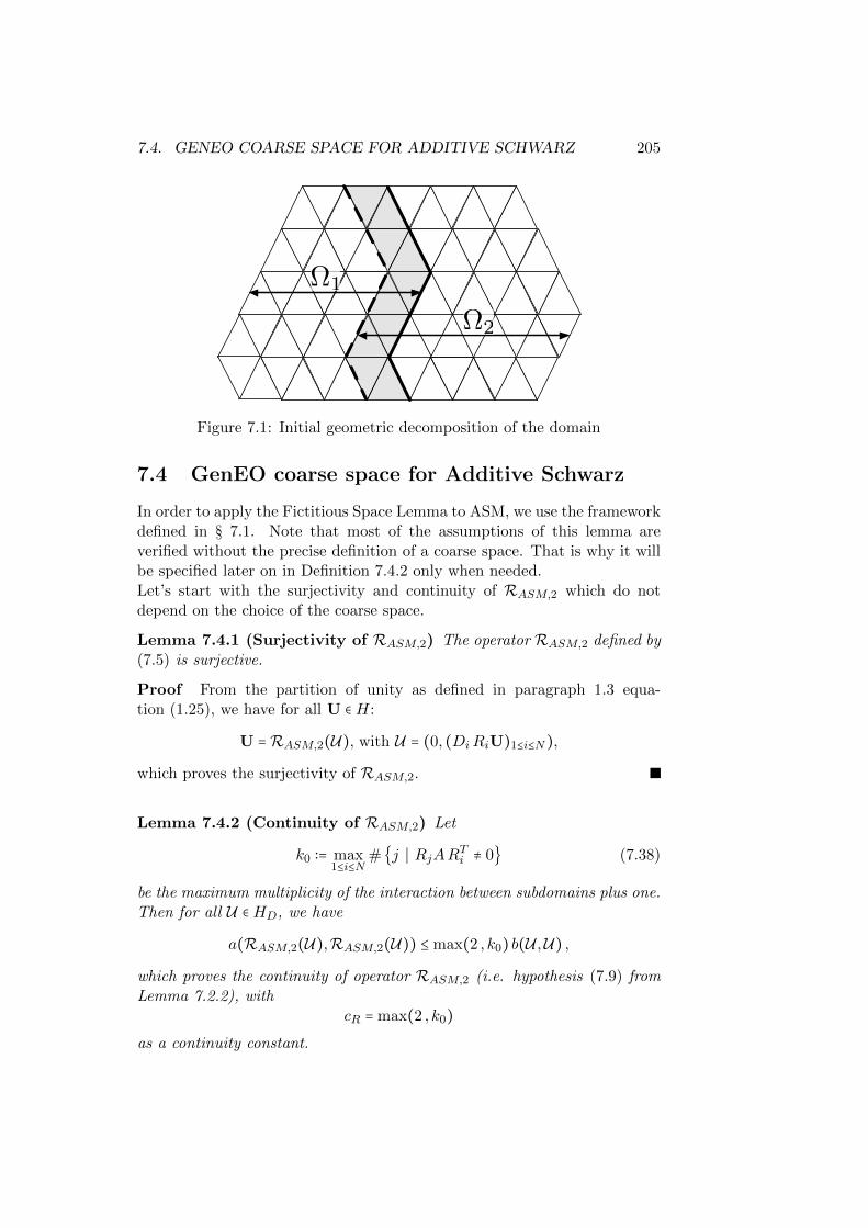
7.4. GENEO COARSE SPACE FOR ADDITIVE SCHWARZ 205
1
2
Figure 7.1: Initial geometric decomposition of the domain
7.4 GenEO coarse space for Additive Schwarz
In order to apply the Fictitious Space Lemma to ASM, we use the frameworkdefined in § 7.1. Note that most of the assumptions of this lemma areverified without the precise definition of a coarse space. That is why it willbe specified later on in Definition 7.4.2 only when needed.Let’s start with the surjectivity and continuity of RASM,2 which do notdepend on the choice of the coarse space.
Lemma 7.4.1 (Surjectivity of RASM,2) The operator RASM,2 defined by(7.5) is surjective.
Proof From the partition of unity as defined in paragraph 1.3 equa-tion (1.25), we have for all U ∈H:
U =RASM,2(U), with U = (0, (DiRiU)1≤i≤N),
which proves the surjectivity of RASM,2.
Lemma 7.4.2 (Continuity of RASM,2) Let
k0 ∶= max1≤i≤N
#j ∣ RjARTi ≠ 0 (7.38)
be the maximum multiplicity of the interaction between subdomains plus one.Then for all U ∈HD, we have
a(RASM,2(U),RASM,2(U)) ≤ max(2 , k0) b(U ,U) ,
which proves the continuity of operator RASM,2 (i.e. hypothesis (7.9) fromLemma 7.2.2), with
cR = max(2 , k0)as a continuity constant.

206 CHAPTER 7. GENEO COARSE SPACE
Proof Let U ∶= (Ui)0≤i≤N ∈HD. Then we have by definition
a(RASM,2(U),RASM,2(U)) = (N
∑i=0
RTi Ui)T
A(N
∑i=0
RTi Ui) (7.39)
and
b(U ,U) =N
∑i=0
(RTi Ui)TA (RTi Ui) . (7.40)
Applying Lemma 7.2.7, with M = N +1, Qi = RTi (0 ≤ i ≤ N) would not yielda sharp estimate. Indeed, we note that R0AR
Ti ≠ 0, 0 ≤ i ≤ N which means
the constant k0 in Lemma 7.2.7 would be equal to N + 1. Thus, we proceedin two steps. Since A is symmetric positive, we have:
(N
∑i=0
RTi Ui)T
A(N
∑i=0
RTi Ui) ≤ 2 ((RT0 U0)TA(RT0 U0)
+(N
∑i=1
RTi Ui)T
A(N
∑i=1
RTi Ui)⎞⎠
(7.41)
We use Lemma 7.2.7 to estimate the last term and we have:
(N
∑i=0
RTi Ui)T
A(N
∑i=0
RTi Ui) ≤ 2 ((RT0 U0)TA(RT0 U0)
+k0
N
∑i=1
(RTi Ui)TA (RTi Ui))
≤ max(2 , k0)N
∑i=0
(RTi Ui)TA (RTi Ui) .
(7.42)
7.4.1 Some estimates for a stable decomposition with RASM,2
We now focus on the stable decomposition, estimate (7.10), which requiresfurther analysis and is dependent on the choice of the coarse space givenhere by its column-matrix form Z0 = RT0 . Nevertheless, we note that someintermediate results, valid for arbitrary coarse space, simplify the require-ment of (7.10). For example, the following lemma which is valid whateverthe choice of Z0 = RT0 .
Lemma 7.4.3 Let U ∈ H and U ∶= (Ui)0≤i≤N ∈ HD such that U =RASM,2(U).Then, we have:
b(U ,U) ≤ 2a(U,U) + (2k0 + 1)N
∑i=1
a(RTi Ui,RTi Ui) . (7.43)

7.4. GENEO COARSE SPACE FOR ADDITIVE SCHWARZ 207
Proof By definition of RASM,2 (see eq. (7.5)) and Cauchy-Schwarz inequal-ity, we have:
b(U ,U) = a(RT0 U0,RT0 U0) +
N
∑i=1
a(RTi Ui,RTi Ui)
= a(U −N
∑i=1
RTi Ui, U −N
∑i=1
RTi Ui) +N
∑i=1
a(RTi Ui,RTi Ui)
≤ 2 [a(U,U) + a(N
∑i=1
RTi Ui,N
∑i=1
RTi Ui)] +N
∑i=1
a(RTi Ui,RTi Ui)
≤ 2
⎡⎢⎢⎢⎢⎣a(U,U) + ∑
1≤i,j≤N/RjARTi ≠0
a(RTi Ui,RTj Uj)
⎤⎥⎥⎥⎥⎦+N
∑i=1
a(RTi Ui,RTi Ui)
Applying Lemma 7.2.7, the middle term can be bounded by
k0
N
∑i=1
a(RTi Ui,RTi Ui) .
and the conclusion follows.
Note that the result (7.43) is insufficient to yield a spectral estimate of theASM preconditioner. We still have to bound from above the subdomain en-ergy terms a(RTi Ui, R
Ti Ui), 1 ≤ i ≤ N , by the global energy term a(U, U).
In order to do this, we first introduce an estimate to a(U, U) from belowin terms of a sum of some local energy terms, see (7.44) and then infer fromit a construction of the coarse space in Definition 7.4.2.
Lemma 7.4.4 Let k1 be the maximal multiplicity of subdomains intersec-tion, i.e. the largest integer m such that there exists m different subdomainswhose intersection has a non zero measure.Then, for all U ∈ RN , we have
N
∑j=1
(RjU)T AjRjU ≤ k1 UTAU = k1 a(U,U) (7.44)
where matrices Aj are defined by eq. (7.37).
Proof This property makes use of the finite element setting of § 7.3. Letuh ∶= ∑k∈N Ukφk, then by definition
aΩ(uh, uh) = UTAU and aΩj(uh, uh) = (RjU)T AjRjU .
Since at most k1 of the subdomains have a non zero measure intersection,the sum ∑Nj=1 aΩj(uh, uh) cannot exceed k1 times aΩ(uh, uh). Let us be moreexplicit in the case of a Darcy equation (7.34). Inequality (7.44) reads:
N
∑j=1∫
ΩjK ∣∇uh∣2 dx ≤ k1∫
ΩK ∣∇uh∣2 dx .

208 CHAPTER 7. GENEO COARSE SPACE
7.4.2 Definition of the GenEO coarse space
All the previous results are valid independently of the choice of the(Uj)1≤j≤N in the decomposition of U and of the coarse space. They can’tgive access to an estimate of the constant cT in the stable decompositionestimate required by condition (7.10) of the Fictitious Space Lemma 7.2.2.But, they are important steps since they enable a local construction of aglobal coarse space so that the constant cT can be chosen, a priori less than1/2, see Lemma 7.4.3. Actually, we see from (7.43) and (7.44) that it issufficient, for some given parameter τ > 0, to define (Uj)1≤j≤N such that
N
∑j=1
a(RTj Uj ,RTj Uj) ≤ τ
N
∑j=1
(RjU)T AjRjU , (7.45)
which can be satisfied by demanding that for all subdomains j we have
a(RTj Uj ,RTj Uj) ≤ τ (RjU)T AjRjU . (7.46)
This estimate will have as a consequence the stability of the decompositionand a short computation shows that we can take cT ∶= (2 + (2k0 + 1)k0 τ)−1
in (7.10). The definition of Uj which satisfy (7.46) for a given threshold τwill be a consequence of the definition of the coarse space.
We now detail the construction of the GenEO coarse space.To start with, we apply the abstract Lemma 7.2.5 in each subdomain to thefollowing generalized eigenvalue problem:
Definition 7.4.1 (Generalized eigenvalue problem) For all subdo-mains 1 ≤ j ≤ N , let
Bj ∶=Dj(RjARTj )Dj .
Let Pj be the projection on range(Aj) parallel to ker(Aj). Consider thegeneralized eigenvalue problem:
Find (Ujk, λjk) ∈ range(Aj) ×R
PjBjPj Ujk = λjk AjUjk .
Define alsoZjτ ∶= ker(Aj)⊕SpanUjk∣ λjk > τ
and the local projection πj on Zjτ parallel to SpanUjk∣ λjk ≤ τ .
With these notations, Lemma 7.2.5 translates into:
7.4. GENEO COARSE SPACE FOR ADDITIVE SCHWARZ 209
Lemma 7.4.5 (Intermediate Lemma) For all subdomain 1 ≤ j ≤ N andUj ∈ RNj , we have:
(RTj Dj(Id − πj)Uj)TA (RTj Dj(Id − πj)Uj) ≤ τ UT
j AjUj . (7.47)
We see now that estimate (7.46) can be obtained directly from (7.47) pro-vided that Uj are such that the left-hand sides of (7.46) and (7.47) are thesame, that is
Uj ∶=Dj(Id − πj)RjU. (7.48)
It remains now to define the coarse space component U0 and the coarsespace interpolation operator, such that ∑Nj=0R
Tj Uj = U. From the previous
results we can infer that this decomposition is stable.
Definition 7.4.2 (GenEO Coarse space) The GenEO coarse space isdefined as a sum of local contributions weighted with the partition of unity:
V0 ∶=N
⊕j=1
RTj DjZjτ . (7.49)
Let Z0 ∈ R#N×dim(V0) be a column matrix so that V0 is spanned by itscolumns. We denote its transpose R0 ∶= ZT0 .
Note that for all U0 ∈ V0, we have the following equality:
U0 = RT0 ((R0RT0 )−1)R0 U0 .
Theorem 7.4.1 (GenEO stable decomposition) Let U ∈ RN , for allsubdomain 1 ≤ j ≤ N , we define Uj like in (7.48) and U0 by:
U0 ∶= (R0RT0 )−1R0
⎛⎝N
∑j=1
RTj Dj πjRjU⎞⎠
so that
RT0 U0 ∶=N
∑j=1
RTj Dj πjRjU.
Let cT ∶= (2 + (2k0 + 1)k0 τ)−1 and U denote (Ui)0≤i≤N ∈HD.Then, U is a cT -stable decomposition of U since we have:
RASM,2(U) =N
∑j=0
RTj Uj = U and b(U ,U) ≤ 1
cTUTAU = a(U,U) .

210 CHAPTER 7. GENEO COARSE SPACE
Proof We first check that R(U) = U . By definition, we have:
U =N
∑j=1
RTj DjRjU
=N
∑j=1
RTj Dj πjRjU
´¹¹¹¹¹¹¹¹¹¹¹¹¹¹¹¹¹¹¹¹¹¹¹¹¹¹¹¹¹¹¹¹¹¹¹¹¹¹¹¹¹¹¹¸¹¹¹¹¹¹¹¹¹¹¹¹¹¹¹¹¹¹¹¹¹¹¹¹¹¹¹¹¹¹¹¹¹¹¹¹¹¹¹¹¹¹¹¶RT0 U0
+N
∑j=1
RTj Dj(Id − πj)RjU´¹¹¹¹¹¹¹¹¹¹¹¹¹¹¹¹¹¹¹¹¹¹¹¹¹¹¹¹¹¹¹¹¹¹¹¹¹¹¹¹¹¹¹¹¸¹¹¹¹¹¹¹¹¹¹¹¹¹¹¹¹¹¹¹¹¹¹¹¹¹¹¹¹¹¹¹¹¹¹¹¹¹¹¹¹¹¹¹¹¶
Uj
=N
∑j=0
RTj Uj .
We now prove the second part of the theorem, the stability of the decom-position. By Lemma 7.4.3, we have
b(U ,U) ≤ 2a(U,U) + (2k0 + 1)N
∑i=1
a(RTi Ui,RTi Ui) . (7.50)
Then, by definition of Ui, 1 ≤ i ≤ N in equation (7.48):
a(RTi Ui,RTi Ui) = (RTi Di(Id − πi)RiU)T A (RTi Di(Id − πi)RiU) (7.51)
and by Lemma 7.4.5 we have thus:
a(RTi Ui,RTi Ui) ≤ τ (RiU)T Ai (RiU) .
Summing over all subdomains and using Lemma 7.4.4, we have:
N
∑i=1
a(RTi Ui,RTi Ui) ≤ k1 τ UTAU .
Finally, using (7.50) and (7.51), we have:
b(U ,U) ≤ (2 + (2k0 + 1)k1 τ)UTAU . (7.52)
Combining Lemma 7.4.2 and equation (7.52), we have thus proved
Theorem 7.4.2 The eigenvalues of the two level Schwarz preconditionedsystem satisfy the following estimate
1
2 + (2k0 + 1)k1 τ≤ λ(M−1
ASM2A) ≤ max(2 , k0) .
Due to the definition of the coarse space, we see that the condition numberof the preconditioned problem will not depend on the number of the subdo-mains but only on the parameters k0, k1 and τ . Parameter τ can be chosenarbitrarily small at the expense of a large coarse space.
7.5. HYBRID SCHWARZ WITH GENEO 211
7.5 Hybrid Schwarz with GenEO
Another version of the Schwarz preconditionner, which we will call HybridSchwarz method (HSM) can be also formalized in the framework of the Fic-titious Space Lemma. The coarse space is as before based on the same gener-alized eigensolves. The difference lies in the way the coarse space correctionis applied, see [132] and [183]. Let P0 (see (7.58)) denote the a-orthogonalprojection on the GenEO coarse space V0 defined above, Definition 7.4.2.Let us denote by M−1
ASM the one-level Schwarz method
M−1ASM ∶=
N
∑i=1
RTi (RiARTi )−1Ri .
Following [132], the hybrid Schwarz preconditioner is defined as follows:
M−1HSM ∶= RT0 (R0AR
T0 )−1R0 + (Id − P0)M−1
ASM(Id − P T0 ) . (7.53)
We shall see at the end how to implement efficiently this preconditioner ina preconditioned conjugate gradient method (PCG).
We first study the spectral properties of this preconditioner. In order toapply the Fictitious Space Lemma 7.2.2, it suffices in the previous set up tomodify the linear operator R (7.5) and replace it by the following definition.
Definition 7.5.1 For U = (Ui)0≤i≤N , RHSM ∶HD Ð→H is defined by
RHSM(U) ∶= RT0 U0 +N
∑i=1
(Id − P0)RTi Ui . (7.54)
We check the assumptions of the Fictitious Space Lemma when RHSM re-places RASM,2 in Definition 7.1.1. This will give us the condition numberestimate (7.57).
Lemma 7.5.1 (Surjectivity of RHSM) The operator RHSM is surjec-tive.
Proof For all U ∈H, we have:
U = P0 U + (Id − P0)U = P0 U +N
∑i=1
(Id − P0)RTi DiRiU .
Since P0 U ∈ V0, there exists U0 ∈ R#N0 such that P0 U = RT0 U0. Thus, wehave
U = RT0 U0 +N
∑i=1
(Id − P0)RTi (DiRiU) ,

212 CHAPTER 7. GENEO COARSE SPACE
or, in other words
RHSM(U0, (DiRiU)1≤i≤N) = U .
which proves the surjectivity.
Lemma 7.5.2 (Continuity of RHSM) Let k0 be defined as in (7.38).Then, for all U = (Ui)0≤i≤N ∈HD, the following estimate holds
a(RHSM(U),RHSM(U)) ≤ k0 b(U ,U). (7.55)
Proof Since P0 and Id − P0 are a-orthogonal projections, we have alsomaking use of Lemma 7.2.7:
a(RHSM(U),RHSM(U)) = a(RT0 U0,RT0 U0)
+a((Id − P0)N
∑i=1
RTi Ui, (Id − P0)N
∑i=1
RTi Ui)
≤ a(RT0 U0, RT0 U0) + a(
N
∑i=1
RTi Ui,N
∑i=1
RTi Ui)
≤ a(RT0 U0, RT0 U0) + k0
N
∑i=1
a(RTi Ui,RTi Ui)
≤ k0
N
∑i=0
a(RTi Ui,RTi Ui) = k0 b(U ,U) .
Lemma 7.5.3 (Stable decomposition with RHSM) Let U ∈ H. For1 ≤ j ≤ N , we define:
Uj ∶=Dj (Id − πj)Rj U
and U0 ∈ RN0 such that:RT0 U0 = P0 U .
We define U ∶= (Ui)1≤i≤N ∈HD.Then, we have
RHSM(U) = U
and the stable decomposition property is verified
b(U ,U) ≤ (1 + k1 τ)a(U,U). (7.56)
Proof We first check that we have indeed a decomposition, i.e. that theequality RHSM(U) = U holds. Note that for all 1 ≤ j ≤ N we have
RTj Dj πj Rj U ∈ V0 ⇒ (Id − P0)RTj Dj πj Rj U = 0 .
7.5. HYBRID SCHWARZ WITH GENEO 213
We have:
U = P0U + (Id − P0)U = P0U + (Id − P0)N
∑j=1
RTj Dj Rj U
= P0 U + (Id − P0)N
∑j=1
RTj Dj Rj U
= RT0 U0 + (Id − P0)N
∑j=1
RTj Dj (Id − πj)Rj U =RHSM(U) .
The last thing to do is to check the stability of this decomposition. UsingLemma 7.4.5, then Lemma 7.4.4 and the fact that P0 is a a-orthogonalprojection, we have
b(U ,U) = a(RT0 U0,RT0 U0)
+N
∑j=1
a(RTj Dj (Id − πj)Rj U´¹¹¹¹¹¹¹¹¹¹¹¹¹¹¹¹¹¹¹¹¹¹¹¹¹¹¹¹¹¹¹¹¹¹¹¹¹¹¹¹¹¹¹¹¹¹¹¹¸¹¹¹¹¹¹¹¹¹¹¹¹¹¹¹¹¹¹¹¹¹¹¹¹¹¹¹¹¹¹¹¹¹¹¹¹¹¹¹¹¹¹¹¹¹¹¹¹¶
Uj
, RTj Dj (Id − πj)Rj U´¹¹¹¹¹¹¹¹¹¹¹¹¹¹¹¹¹¹¹¹¹¹¹¹¹¹¹¹¹¹¹¹¹¹¹¹¹¹¹¹¹¹¹¹¹¹¹¹¸¹¹¹¹¹¹¹¹¹¹¹¹¹¹¹¹¹¹¹¹¹¹¹¹¹¹¹¹¹¹¹¹¹¹¹¹¹¹¹¹¹¹¹¹¹¹¹¹¶
Uj
)
≤ a(P0U, P0U) + τN
∑j=1
(RjU)T Aj (RjU)
≤ a(U,U) + k1 τa(U,U) ≤ (1 + k1 τ)a(U,U) .
Previous lemmas lead to the condition number estimate of the algorithm:
Theorem 7.5.1 (Hybrid Schwarz algorithm) Let τ be a user-definedparameter to build the GenEO coarse space as in Definition 7.4.1.The eigenvalues of the hybrid Schwarz preconditioned system satisfy the fol-lowing estimate
1
1 + k1 τ≤ λ(M−1
HSM A) ≤ k0. (7.57)
Note that a hybrid preconditionner will lead to a better condition num-ber than for the additive one (Theorem 7.4.2) and consequently to a fasterconvergence.
7.5.1 Efficient implementation of the hybrid Schwarzmethod
As it is written in (7.53), the application of the hybrid preconditionerinvolves several applications of the projection P0. We see in this paragraphthat a clever choice of the initial guess in the PCG algorithm reduces thecost of the algorithm, see [132].
Note first that the matrix form of P0 is:
P0 = RT0 (R0ART0 )−1R0A. (7.58)
214 CHAPTER 7. GENEO COARSE SPACE
Indeed, this formula clearly defines a projection since
(RT0 (R0ART0 )−1R0A)2 = RT0 (R0AR
T0 )−1R0AR
T0 (R0AR
T0 )−1R0A
= RT0 (R0ART0 )−1R0A.
This projection is A-orthogonal since for all vectors U , V , we have:
(RT0 (R0ART0 )−1R0AU , V )A = (RT0 (R0AR
T0 )−1R0AU , AV )
= (U , RT0 (R0ART0 )−1R0AV )A .
Finally, the range of RT0 (R0ART0 )−1R0A is V0 since for all U ∈ V0, there
exist W such that U = RT0W and we have:
RT0 (R0ART0 )−1R0AU = RT0 (R0AR
T0 )−1R0AR
T0W = RT0W = U .
From (7.58), we can rewrite definition (7.53) of M−1HSM as:
M−1HSM ∶= P0A
−1 + (Id − P0)M−1ASM(Id − P T0 ) .
Note also that :
P T0 A = ART0 (R0ART0 )−1R0A = AP0 .
These relations yield the following expression for the preconditioned operator
M−1HSMA = P0 + (Id − P0)M−1
ASMA(Id − P0) . (7.59)
When solving the linear system Ax = b with the preconditioned conjugategradient (PCG) preconditioned by M−1
HSM (7.53) the method seeks an ap-proximation to the solution in the Krylov space
Kn(M−1HSMA, r0) ∶= r0,M−1
HSMA r0, . . . , (M−1HSMA)n−1r0
where
r0 ∶=M−1HSM (b −Ax0)
is the initial preconditioned residual. If r0 is chosen so that
P0 r0 = 0 ,
we have a simplification in the expression of the Krylov subspace:
Kn(M−1HSMA, r0) = r0, (Id − P0)M−1
ASMAr0, . . . , ((Id − P0)M−1ASM)n−1r0 .
7.6. FREEFEM++ IMPLEMENTATION 215
This can be easily proved using formula (7.59) and the fact that P 20 = P0:
M−1HSMA r0 = (P0 + (Id − P0)M−1
ASMA(Id − P0)) r0= (Id − P0)M−1
ASMA r0 ,
(M−1HSMA)2 r0 = (P0 + (Id − P0)M−1
ASMA(Id − P0))(Id − P0)M−1ASMA r0
= (Id − P0)M−1ASMA(Id − P0)M−1
ASMA r0
= ((Id − P0)M−1ASMA)2 r0,
⋮
It means that in the PCG method, it is sufficient to consider that the pre-conditioner is
(Id − P0)M−1ASM .
In order to have P0 r0 = 0, we can choose for example
x0 = RT0 (R0ART0 )−1R0 b .
By using (7.53) and (7.58) we see that:
P0M−1HSM = P0R
T0 (R0AR
T0 )−1R0 = RT0 (R0AR
T0 )−1R0
which leads to
P0 r0 = P0M−1HSM(b −ART0 (R0AR
T0 )−1R0 b)
= RT0 (R0ART0 )−1R0 (b −ART0 (R0AR
T0 )−1R0 b)
= 0 .
To sum up, the PCG algorithm (see Algorithm 5 in § 3.3.1) for the HybridSchwarz method takes the form given in Algorithm 8.
7.6 FreeFem++ Implementation
We illustrate the GenEO coarse space on a Darcy problem with two layersof very high and different heterogeneities, see Figure 7.2:
− div(α∇u) = f, in Ω (7.60)
where α ∶ Ω↦ R is defined by:
α =⎧⎪⎪⎪⎨⎪⎪⎪⎩
1.e6 if .2 < y < .41.e5 if .6 < y < .81. else
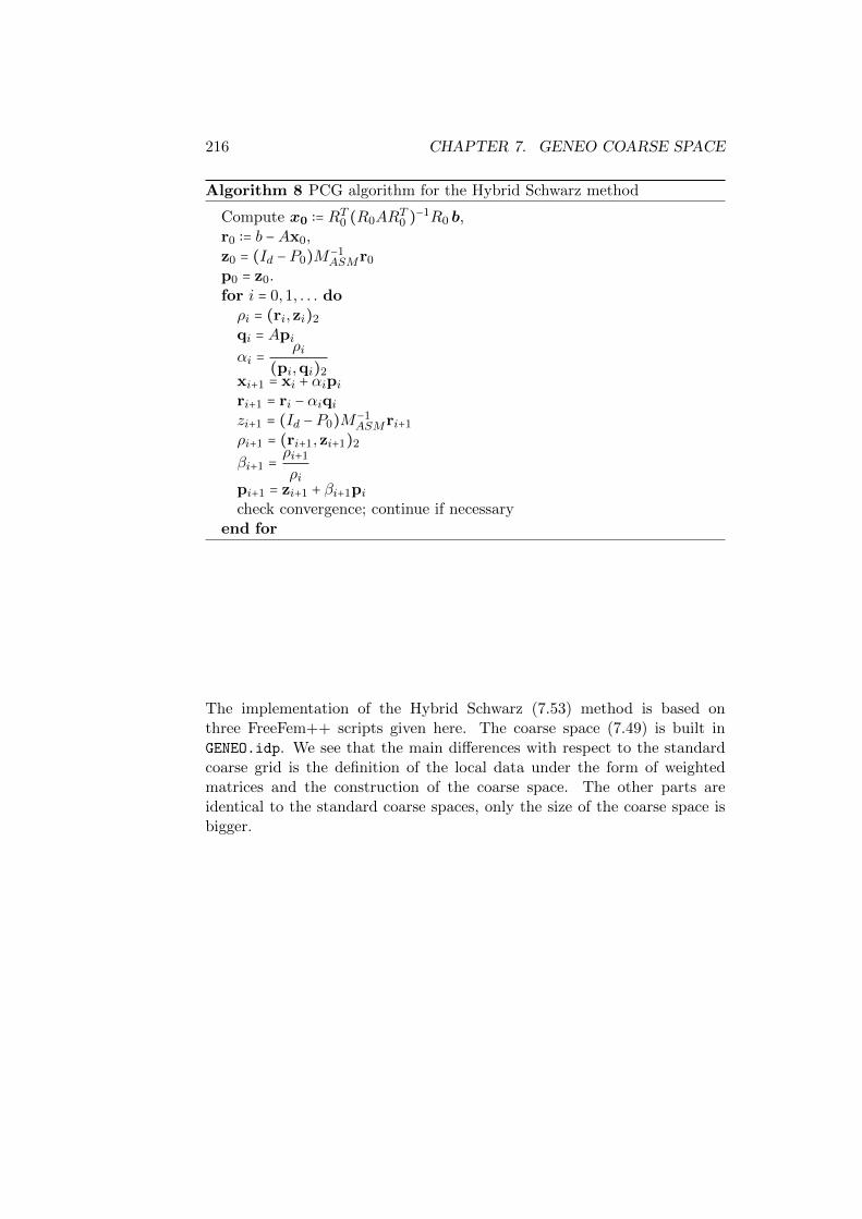
216 CHAPTER 7. GENEO COARSE SPACE
Algorithm 8 PCG algorithm for the Hybrid Schwarz method
Compute x0 ∶= RT0 (R0ART0 )−1R0 b,
r0 ∶= b −Ax0,z0 = (Id − P0)M−1
ASMr0
p0 = z0.for i = 0,1, . . . doρi = (ri,zi)2
qi = Apiαi =
ρi(pi,qi)2
xi+1 = xi + αipiri+1 = ri − αiqizi+1 = (Id − P0)M−1
ASMri+1
ρi+1 = (ri+1,zi+1)2
βi+1 =ρi+1
ρipi+1 = zi+1 + βi+1picheck convergence; continue if necessary
end for
The implementation of the Hybrid Schwarz (7.53) method is based onthree FreeFem++ scripts given here. The coarse space (7.49) is built inGENEO.idp. We see that the main differences with respect to the standardcoarse grid is the definition of the local data under the form of weightedmatrices and the construction of the coarse space. The other parts areidentical to the standard coarse spaces, only the size of the coarse space isbigger.
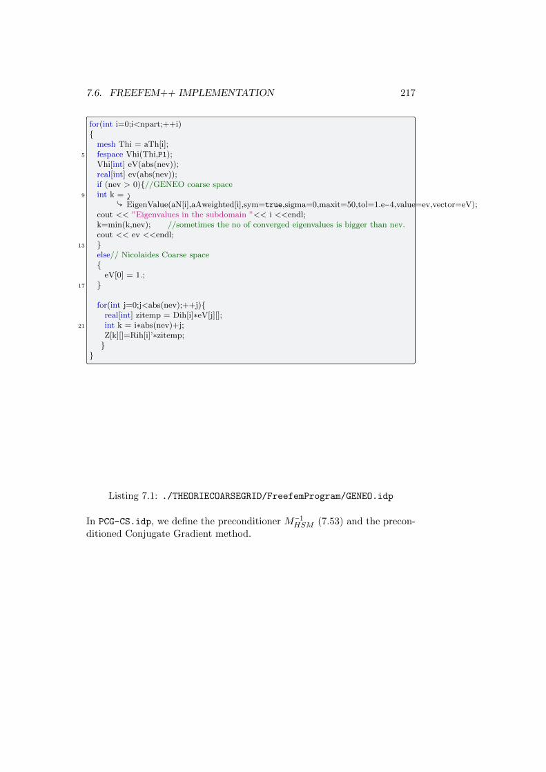
7.6. FREEFEM++ IMPLEMENTATION 217
for(int i=0;i<npart;++i)
mesh Thi = aTh[i];5 fespace Vhi(Thi,P1);
Vhi[int] eV(abs(nev));real[int] ev(abs(nev));if (nev > 0)//GENEO coarse space
9 int k = ⤸Ç EigenValue(aN[i],aAweighted[i],sym=true,sigma=0,maxit=50,tol=1.e−4,value=ev,vector=eV);
cout << ”Eigenvalues in the subdomain ”<< i <<endl;k=min(k,nev); //sometimes the no of converged eigenvalues is bigger than nev.cout << ev <<endl;
13 else// Nicolaides Coarse space
eV[0] = 1.;17
for(int j=0;j<abs(nev);++j)real[int] zitemp = Dih[i]∗eV[j][];
21 int k = i∗abs(nev)+j;Z[k][]=Rih[i]’∗zitemp;
Listing 7.1: ./THEORIECOARSEGRID/FreefemProgram/GENEO.idp
In PCG-CS.idp, we define the preconditioner M−1HSM (7.53) and the precon-
ditioned Conjugate Gradient method.

218 CHAPTER 7. GENEO COARSE SPACE
func real[int] AS2(real[int] & r)real[int] z = Q(r);
8 real[int] aux = AS(r);z += aux;return z;
12 func real[int] BNN(real[int] &u) // precond BNN
real[int] aux1 = Q(u);real[int] aux2 = P(u);
16 real[int] aux3 = AS(aux2);//aux3 = AS(P(u))aux2 = PT(aux3);// aux2 = PT(AS(P(u)))aux2 += aux1;// aux2 = Q(u) + PT(AS(P(u)))
return aux2;20
/∗# fin BNNPrecond #∗//∗# debutCGSolve #∗/func real[int] myPCG(real[int] xi,real eps, int nitermax)
24 ofstream filei(”Convprec.m”); // Matlab convergence history fileofstream fileignu(”Convprec.gnu”); // Gnuplot convergence history file
Vh r, un, p, zr, zrel, rn, w, er;28 un[] = xi;
r[] = A(un[]);r[] −= rhsglobal[];r[] ∗= −1.0;
32 zr[] = BNN(r[]);real resinit=sqrt(zr[]’∗zr[]);p = zr;for(int it=0;it<nitermax;++it)
36 plot(un,value=1,wait=1,fill=1,dim=3,cmm=”Approximate solution at ⤸
Ç iteration ”+it);real relres = sqrt(zr[]’∗zr[])/resinit;cout << ”It: ”<< it << ” Relative residual = ” << relres << endl;
40 int j = it+1;filei << ”relres(”+j+”)=” << relres << ”;” << endl;fileignu << relres << endl;if(relres < eps)
44 cout << ”CG has converged in ” + it + ” iterations ” << endl;cout << ”The relative residual is ” + relres << endl;break;
48 w[] = A(p[]);real alpha = r[]’∗zr[];real aux2 = alpha;
52 real aux3 = w[]’∗p[];alpha /= aux3; // alpha = (rj,zj)/(Apj,pj);un[] += alpha∗p[]; // xj+1 = xj + alpha∗p;r[] −= alpha∗w[]; // rj+1 = rj − alpha∗Apj;
56 zr[] = BNN(r[]); // zj+1 = M−1∗rj+1;real beta = r[]’∗zr[];beta /= aux2; // beta = (rj+1,zj+1)/(rj,zj);p[] ∗= beta;
60 p[] += zr[];
return un[];
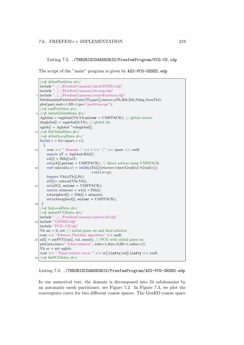
7.6. FREEFEM++ IMPLEMENTATION 219
Listing 7.2: ./THEORIECOARSEGRID/FreefemProgram/PCG-CS.idp
The script of the ”main” program is given by AS2-PCG-GENEO.edp
/∗# debutPartition #∗/include ”../../FreefemCommon/dataGENEO.edp”include ”../../FreefemCommon/decomp.idp”
4 include ”../../FreefemCommon/createPartition.idp”SubdomainsPartitionUnity(Th,part[],sizeovr,aTh,Rih,Dih,Ndeg,AreaThi);plot(part,wait=1,fill=1,ps=”partition.eps”);/∗# endPartition #∗/
8 /∗# debutGlobalData #∗/Aglobal = vaglobal(Vh,Vh,solver = UMFPACK); // global matrixrhsglobal[] = vaglobal(0,Vh); // global rhs
uglob[] = Aglobal−1∗rhsglobal[];12 /∗# finGlobalData #∗/
/∗# debutLocalData #∗/for(int i = 0;i<npart;++i)
16 cout << ” Domain :” << i << ”/” << npart << endl;matrix aT = Aglobal∗Rih[i]’;aA[i] = Rih[i]∗aT;set(aA[i],solver = UMFPACK); // direct solvers using UMFPACK
20 varf valocal(u,v) = int2d(aTh[i])(eta∗u∗v+ka∗(Grad(u)’∗Grad(v)))+on(1,u=g);
fespace Vhi(aTh[i],P1);aN[i]= valocal(Vhi,Vhi);
24 set(aN[i], solver = UMFPACK);matrix atimesxi = aA[i] ∗ Dih[i];aAweighted[i] = Dih[i] ∗ atimesxi;set(aAweighted[i], solver = UMFPACK);
28 /∗# finLocalData #∗//∗# debutPCGSolve #∗/include ”../../FreefemCommon/matvecAS.idp”
32 include ”GENEO.idp”include ”PCG−CS.idp”Vh un = 0, sol; // initial guess un and final solutioncout << ”Schwarz Dirichlet algorithm” << endl;
36 sol[] = myPCG(un[], tol, maxit); // PCG with initial guess unplot(sol,cmm=” Final solution”, wait=1,dim=3,fill=1,value=1);Vh er = sol−uglob;cout << ” Final relative error: ” << er[].linfty/sol[].linfty << endl;
40 /∗# finPCGSolve #∗/
Listing 7.3: ./THEORIECOARSEGRID/FreefemProgram/AS2-PCG-GENEO.edp
In our numerical test, the domain is decomposed into 24 subdomains byan automatic mesh partitioner, see Figure 7.2. In Figure 7.3, we plot theconvergence curve for two different coarse spaces. The GenEO coarse space

220 CHAPTER 7. GENEO COARSE SPACEIsoValue-52630.626316.878948.41315801842122368432894753421063947384473695000015526336052646578967105277631598157908684229210541.05263e+06
Figure 7.2: Diffusion coefficient (left) and subdomain partition (right)
with two degrees of freedom per subdomain yields a convergence in 18 itera-tions whereas a coarse space built from subdomain-wise constant functions,Nicolaides coarse space, yields a convergence in almost 120 iterations.
0 20 40 60 80 100 12010−7
10−6
10−5
10−4
10−3
10−2
10−1
100
Iterations
Resid
ual
NicolaidesGenEO
Figure 7.3: Comparison between Nicolaides and GenEO coarse spaces
7.7 SORAS-GenEO-2 coarse space for OptimizedSchwarz method
7.7.1 Symmetrized ORAS method
The purpose of this section is to define a general framework for buildingadaptive coarse space for Optimized Schwarz Methods (OSM, see § 2) fordecomposition into overlapping subdomains. We show that we can achievethe same robustness that what was done in this chapter for Schwarz [178]and FETI-BDD [179] domain decomposition methods with GenEO (Gener-alized Eigenvalue in the Overlap) coarse spaces. For this, a non standardsymmetric variant of the ORAS method as well as two generalized eigenvalueproblems are introduced in [106].
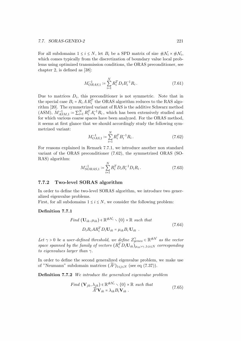
7.7. SORAS-GENEO-2 221
For all subdomains 1 ≤ i ≤ N , let Bi be a SPD matrix of size #Ni × #Ni,which comes typically from the discretization of boundary value local prob-lems using optimized transmission conditions, the ORAS preconditioner, seechapter 2, is defined as [38]:
M−1ORAS,1 ∶=
N
∑i=1
RTi DiB−1i Ri . (7.61)
Due to matrices Di, this preconditioner is not symmetric. Note that inthe special case Bi = RiARTi the ORAS algorithm reduces to the RAS algo-rithm [20]. The symmetrized variant of RAS is the additive Schwarz method(ASM), M−1
ASM,1 ∶= ∑Ni=1RTi A
−1i Ri , which has been extensively studied and
for which various coarse spaces have been analyzed. For the ORAS method,it seems at first glance that we should accordingly study the following sym-metrized variant:
M−1OAS,1 ∶=
N
∑i=1
RTi B−1i Ri . (7.62)
For reasons explained in Remark 7.7.1, we introduce another non standardvariant of the ORAS preconditioner (7.62), the symmetrized ORAS (SO-RAS) algorithm:
M−1SORAS,1 ∶=
N
∑i=1
RTi DiB−1i DiRi . (7.63)
7.7.2 Two-level SORAS algorithm
In order to define the two-level SORAS algorithm, we introduce two gener-alized eigenvalue problems.First, for all subdomains 1 ≤ i ≤ N , we consider the following problem:
Definition 7.7.1
Find (Uik, µik) ∈ R#Ni ∖ 0 ×R such that
DiRiARTi DiUik = µikBiUik .
(7.64)
Let γ > 0 be a user-defined threshold, we define Zγgeneo ⊂ R#N as the vectorspace spanned by the family of vectors (RTi DiUik)µik>γ ,1≤i≤N correspondingto eigenvalues larger than γ.
In order to define the second generalized eigenvalue problem, we make useof ”Neumann” subdomain matrices (Aj)1≤j≤N (see eq (7.37)).
Definition 7.7.2 We introduce the generalized eigenvalue problem
Find (Vjk, λjk) ∈ R#Ni ∖ 0 ×R such that
AiVik = λikBiVik .(7.65)

222 CHAPTER 7. GENEO COARSE SPACE
Let τ > 0 be a user-defined threshold, we define Zτgeneo ⊂ R#N as the vector
space spanned by the family of vectors (RTi DiVik)λik<τ ,1≤i≤N correspondingto eigenvalues smaller than τ .
We are now ready to define the SORAS two level preconditioner
Definition 7.7.3 (The SORAS-GenEO-2 preconditioner) Let P0 de-note the A-orthogonal projection on the coarse space
ZGenEO-2 ∶= Zγgeneo⊕Zτgeneo ,
the two-level SORAS-GenEO-2 preconditioner is defined as follows:
M−1SORAS,2 ∶= P0A
−1 + (Id − P0)N
∑i=1
RTi DiB−1i DiRi(Id − P T0 ) . (7.66)
This definition is reminiscent of the balancing domain decomposition pre-conditioner [132] introduced for Schur complement based methods. Notethat the coarse space is now defined by two generalized eigenvalue problemsinstead of one in [178, 179] for ASM and FETI-BDD methods. We have thefollowing theorem
Theorem 7.7.1 (Spectral estimate for the SORAS-GenEO-2 preconditioner)Let k0 be the maximal multiplicity of the subdomain intersections (seeeq. (7.38)), γ, τ > 0 be arbitrary constants used in Definitions 7.7.2 and7.7.3 .Then, the eigenvalues of the two-level preconditioned operator satisfy thefollowing spectral estimate
1
1 + k0
τ
≤ λ(M−1SORAS,2A) ≤ max(1, k0 γ)
where λ(M−1SORAS,2A) is an eigenvalue of the preconditioned operator.
The proof is based on the fictitious space lemma [150].
Remark 7.7.1 An analysis of a two-level version of the preconditionerM−1OAS (7.63) following the same path yields the following two generalized
eigenvalue problems:
Find (Ujk, µjk) ∈ R#Ni ∖ 0 ×R such thatAiUik = µikBiUik ,
andFind (Vjk, λjk) ∈ R#Ni ∖ 0 ×R such that
AiVik = λikDiBiDiVik ..
7.7. SORAS-GENEO-2 223
In the general case for 1 ≤ i ≤ N , matrices Di may have zero entries forboundary degrees of freedom since they are related to a partition of unity.Moreover very often matrices Bi and Ai differ only by the interface condi-tions that is for entries corresponding to boundary degrees of freedom. There-fore, matrix DiBiDi on the right hand side of the last generalized eigenvalueproblem is not impacted by the choice of the interface conditions of the onelevel optimized Schwarz method. This cannot lead to efficient adaptive coarsespaces.
7.7.3 Nearly Incompressible elasticity
Although our theory does not apply in a straightforward manner to saddlepoint problems, we use it for these difficult problems for which it is notpossible to preserve both symmetry and positivity of the problem. Notethat generalized eigenvalue problems (7.89) and (7.66) still make sense if Ais the matrix of a saddle point problem and matrices Bi and Ai are properlydefined for each subdomain 1 ≤ i ≤ N . The new coarse space was testedquite successfully on Stokes and nearly incompressible elasticity problemswith a discretization based on saddle point formulations in order to avoidlocking phenomena. We first report 2D results for the latter case wherecomparisons are made with other methods in terms of iteration counts only.The mechanical properties of a solid can be characterized by its Youngmodulus E and Poisson ratio ν or alternatively by its Lame coefficients λand µ. These coefficients relate to each other by the following formulas:
λ = Eν
(1 + ν)(1 − 2ν) and µ = E
2(1 + ν) . (7.67)
The variational problem consists in finding (uh, ph) ∈ Vh ∶= Pd2 ∩H10(Ω) × P1
such that for all (vh, qh) ∈ Vh⎧⎪⎪⎪⎪⎨⎪⎪⎪⎪⎩
∫Ω 2µε(uh) ∶ ε(vh)dx − ∫Ω phdiv (vh)dx = ∫Ω fvhdx
− ∫Ω div (uh)qhdx − ∫Ω1λphqh = 0
(7.68)
Matrix Ai arises from the variational formulation (7.69) where the integra-tion over domain Ω is replaced by the integration over subdomain Ωi andfinite element space Vh is restricted to subdomain Ωi. Matrix Bi correspondsto a Robin problem and is the sum of matrix Ai and of the matrix of thefollowing variational formulation restricted to the same finite element space:
∫∂Ωi∖∂Ω
2αµ(2µ + λ)λ + 3µ
uh ⋅ vh with α = 10 in our test.
We test various domain decomposition methods for a heterogeneous beamof eight layers of steel (E1, ν1) = (210 ⋅ 109,0.3) and rubber (E2, ν2) = (0.1 ⋅

224 CHAPTER 7. GENEO COARSE SPACE
Figure 7.4: 2D Elasticity: coefficient distribution of steel and rubber.
Table 7.1: 2D Elasticity. GMRES iteration counts for a solid made of steeland rubber. Simulations made with FreeFem++ [108]
AS SORAS AS+ZEM SORAS +ZEM AS-GenEO SORAS geneo2d.o.f N iter. iter. iter. dim iter. dim iter. dim iter. dim
35841 8 150 184 117 24 79 24 110 184 13 14570590 16 276 337 170 48 144 48 153 400 17 303
141375 32 497 >1000 261 96 200 96 171 800 22 561279561 64 >1000 >1000 333 192 335 192 496 1600 24 855561531 128 >1000 >1000 329 384 400 384 >1000 2304 29 1220
1077141 256 >1000 >1000 369 768 >1000 768 >1000 3840 36 1971
109,0.4999), see Figure 7.4. The beam is clamped on its left and right sides.Iteration counts for a relative tolerance of 10−6 are given in Table 7.1. Wecompare the one level Additive Schwarz (AS) and SORAS methods, thetwo level AS and SORAS methods with a coarse space consisting of rigidbody motions which are zero energy modes (ZEM) and finally AS with aGenEO coarse space and SORAS with the GenEO-2 coarse space defined inDefinition 7.7.3 with τ = 0.4 and γ = 103. Columns dim refer to the totalsize of the coarse space of a two-level method. Eigenvalue problem (7.66)accounts for roughly 90% of the GenEO-2 coarse space size.We performed large 3D simulations on 8192 cores of a IBM/Blue Gene Qmachine with 1.6 GHz Power A2 processors for both elasticity (200 millionsof d.o.f’s in 200 sec.) and Stokes (200 millions of d.o.f’s in 150 sec. )equations. Computing facilities were provided by an IDRIS-GENCI project.
7.8. BALANCING NEUMANN-NEUMANN 225
7.8 Balancing Neumann-Neumann
In the same spirit as in the previous sections of this chapter, the purposeis to reformulate the classical Neumann-Neumann algorithms in theframework of the Fictitious Space Lemma. Note that GenEO versions ofthe Neumann-Neumann and FETI algorithms were first introduced in [179]and then analyzed in [180].
We first recall the Neumann-Neumann algorithm introduced in chapter 6.The aim is to solve the substructured system (6.40)
SUΓ =GΓ ∈ R#NΓ (7.69)
where S is the Schur complement of the global matrix (6.39). This systemis defined on the interfaces degrees of freedom indexed by NΓ. The set NΓ
is decomposed into subdomain interfaces degrees of freedom:
NΓ =N
⋃i=1
NΓi .
For each subdomain 1 ≤ i ≤ N , let RΓi be the restriction operator from theskeleton R#NΓ onto the subdomain interface R#NΓi and DΓi ∈ R#NΓi
×#NΓi
be invertible diagonal matrices so that we have the following partition ofunity on the skeleton:
N
∑i=1
RTΓiDΓiRΓi = IR#NΓ . (7.70)
In this context, a Schwarz preconditioner for problem (7.70):
M−1ASMS ∶=
N
∑i=1
RTΓi(RΓiSRTΓi)
−1RΓi
has been considered in [97, 98]. The Neumann-Neumann (NN) precondi-tioner works differently, see Definition 6.4.1. It is based on a decompositionof the global Schur complement operator S into a sum of symmetric positive(but usually not definite) operators. Let (Si)1≤i≤N be given by (6.41), recallthat we have:
S =N
∑i=1
Si .
In § 6.4, we have defined local operators for 1 ≤ i ≤ N :
Si ∶= RΓi SiRTΓi
where Si ∈ R#NΓi×#NΓi are subdomain contributions. Thus, we have
S =N
∑i=1
RTΓiSiRΓi (7.71)

226 CHAPTER 7. GENEO COARSE SPACE
and equation (7.70) can be re-written as
N
∑i=1
RTΓiSiRΓiUΓ =GΓ . (7.72)
When the operators Si are invertible, the Neumann-Neumann precondi-tioner [13] is defined as:
M−1NN ∶=
N
∑i=1
RTΓiDΓiS−1i DΓiRΓi . (7.73)
7.8.1 Easy Neumann-Neumann
We start with the analysis of the one-level Neumann-Neumann (NN) methodassuming that the local matrices Si are invertible.
Definition 7.8.1 (NN components in the Fictitious Space Lemma)In the framework of the Fictitious Space Lemma 7.2.2 we define
• The space of the skeleton
H ∶= R#NΓ
endowed with the standard Euclidean scalar product and the bilinearform a ∶H ×H ↦ R
a(U ,V ) ∶= (SU , V ) , ∀U , V ∈H .
• The product space of the subdomain interfaces
HD ∶=N
∏i=1
RNΓi
endowed with the standard Euclidean scalar product and the bilinearform b
b ∶HD ×HD Ð→ R
((Ui)1≤i≤N , (Vi)1≤i≤N) z→N
∑i=1
(SiUi,Vi) .
• The linear operator RNN as
RNN ∶HD Ð→H
(Ui)1≤i≤N ↦N
∑i=1
RTΓiDΓiUi(7.74)

7.8. BALANCING NEUMANN-NEUMANN 227
With these notations, the preconditioner M−1NN is given by RNNB−1R∗
NN .
Note that the operatpor RNN is surjective since from (7.71), we have forall U ∈H:
U =N
∑i=1
RTΓiDΓiRΓiU =RNN((RΓiU)1≤i≤N) .
Contrarily to the Schwarz method, the stable decomposition is easily checkedand is satisfied with cT = 1. Indeed, let U ∈ H, we have the natural decom-position U = ∑Ni=1R
TΓiDΓiRΓiU . In other words, let U ∶= (RΓiU)1≤i≤N , we
have U =RNN(U). By definition of the bilinear form b we have:
b(U ,U) =N
∑i=1
(SiRΓiU , RΓiU) = (N
∑i=1
RTΓiSiRΓiU , U) = (SU ,U) = a(U ,U) .
We now study the stability of RNN which is more intricate.
Lemma 7.8.1 (Continuity of the operator RNN) Let
k2 ∶= max1≤i≤N
#j ∣ RΓjSRTΓi ≠ 0 (7.75)
be the maximum multiplicity of the interaction between sub-interfaces via theSchur complement operator. Let also
τmax ∶= max1≤i≤N
maxUi∈R#Ni/0
(SRTΓiDΓiUi, RTΓiDΓiUi)
(SiUi, Ui). (7.76)
Then, for all U ∈HD we have:
a(RNN(U), RNN(U)) ≤ cR b(U , U) .
with cR ∶= k2 τmax.
Proof Let U = (Ui)1≤i≤N ∈HD, then
a(RNN(U),RNN(U)) =⎛⎝S(
N
∑i=1
RTΓiDΓiUi) ,N
∑j=1
RTΓjDΓjUj⎞⎠.
It is sufficient to apply Lemma 7.2.7 where matrix A is S to get
a(RNN(U),RNN(U)) ≤ k2
N
∑i=1
(SRTΓiDΓiUi, RTΓiDΓiUi) (7.77)
We now estimate the continuity constant of the linear operator RNN . From(7.78) and the definition of τmax, we have:
a(RNN(U), RNN(U)) ≤ k2
N
∑i=1
(SRTΓiDΓiUi, RTΓiDΓiUi)
≤ k2 τmaxN
∑i=1
(SiUi, Ui) = k2 τmax b(U , U) .

228 CHAPTER 7. GENEO COARSE SPACE
i
Figure 7.5: Interface skeleton and support of SRTΓi .
Note that k2 is typically larger than k0 defined in (7.38) as the numberof neighbors of a subdomain. This is due to the sparsity pattern of S asillustrated in Figure 7.5 for a P1 finite element discretization. The entriesof SRTΓi are not zero on the interfaces drawn with a continuous line. On
the dashed interfaces, the entries of SRTΓi are zero. Note that k2 is typicallythe number of neighbors of neighbors of a subdomain as seen it can be seenfrom this equality
k2 = max1≤i≤N
#j ∣N
∑k=1
RΓjRTΓkSkRΓk R
TΓi ≠ 0 (7.78)
obtained using formula (7.72) in the definition of k2 (7.76).
By applying the Fictitious Space Lemma 7.2.2 we have just proved:
Theorem 7.8.1 (Spectral estimate for Easy Neumann-Neumann)Let τmax be defined by (7.77) and k2 by (7.76). Then, the eigenvalues ofthe Neumann-Neumann preconditioned (7.74) system satisfy the followingestimate
1 ≤ λ(M−1NN S) ≤ k2 τmax .
This result is of little practical use since it assumes that the local Neumannsubproblems are well-posed which is not always the case. Moreover, we havestudied only the one level method.We address the former issue in the next section and a GenEO coarse spaceconstruction in § 7.8.3.

7.8. BALANCING NEUMANN-NEUMANN 229
7.8.2 Neumann-Neumann with ill-posed subproblems
In the case of a Poisson problem and for floating subdomains (subdomainswhich do not touch the boundary of the global domain), constant functionsare in the kernel of the Neumann subproblems and thus the Schur com-plement Si has a non trivial kernel. For elasticity problems, one has toconsider rigid body motions. Thus, we have to take into account the possi-bility to have a non zero kernel for the local Schur complement Si, 1 ≤ i ≤ Nsince for stationary problems, it will often be the case. For each subdomain1 ≤ i ≤ N , the operator Si is symmetric and we have the orthogonal direct
sum (denoted by the symbol⊥⊕):
RNΓi = kerSi⊥⊕ rangeSi
and we denote by
Pi the orthogonal projection from RNΓi on kerSi and parallel to rangeSi .
Note that Si induces an isomorphism from rangeSi into itself whose inversewill be denoted by S†
i ,
S†i ∶ rangeSi → rangeSi .
In order to capture the part of the solution that will come from the local ker-nels Si (1 ≤ i ≤ N), let Zi be a rectangular matrix of size #NΓi ×dim(kerSi)whose columns are a basis of kerSi. We form a rectangular matrix Z0 ofsize #NΓ ×∑Ni=1 dim(kerSi) by concatenation of the Zi’s:
Z0 ∶= (RTΓiDΓiZi)1≤i≤N .
Let W0 be the vector space spanned by the columns of Z0, we introduce the
projection P0 from R#NΓ on W0 and which is S orthogonal.
Note that if Z0 is full rank, the matrix form of the linear operator P0 is
P0 = Z0(ZT0 SZ0)−1ZT0 S . (7.79)
Definition 7.8.2 (Balancing NN and the Fictitious Space Lemma)In the framework of the Fictitious Space Lemma 7.2.2 we define
• The Hilbert spaceH ∶= RNΓ
with its standard Euclidean scalar product denoted (⋅, ⋅) is also endowedwith the bilinear form a defined as:
a(U,V) ∶= VT SU .
230 CHAPTER 7. GENEO COARSE SPACE
• The product space defined by
HD ∶=W0 ×N
∏i=1
rangeSi
with its standard Euclidean scalar product denoted (⋅, ⋅) is also endowedwith the bilinear form b defined as:
b ∶HD ×HD Ð→ R
((Ui)0≤i≤N , (Vi)0≤i≤N) z→ VT0 SU0 +
N
∑i=1
VTi SiUi .
• The linear operator RBNN is defined as:
RBNN ∶HD Ð→H
(Ui)0≤i≤N z→U0 + (Id − P0)N
∑i=1
RTΓiDΓiUi .(7.80)
Lemma 7.8.2 (Balancing Neumann-Neumann preconditioner)Using the notations in Definition 7.8.2, the Balancing Neumann-Neummanpreconditioner is
RBNNB−1R∗BNN = P0 S−1 + (Id − P0)
N
∑i=1
RTΓiDΓiS†i (Id − Pi)DΓiRΓi(Id − P0)T .
(7.81)
Proof We first need to find R∗BNN . By definition, we have:
R∗BNN ∶H Ð→HD
Uz→R∗BNN(U) ,
such that∀V ∈HD , VTR∗
BNN(U) =RBNN(V)TU .
For all V ∶= (Vi)0≤i≤N ∈HD, the above equation is
VT0R∗
BNN(U)0 +N
∑i=1
VTi R∗
BNN(U)i = (V0 + (Id − P0)N
∑i=1
RTΓiDΓiVi)TU
= VT0 U +
N
∑i=1
VTi DΓiRΓi(Id − P0)TU .
SinceHD is a product space, for arbitrary V0 ∈W0 and Vi ∈ R#NΓi (1 ≤ i ≤ N)we can identify each term in the sum. Thus we have:
R∗BNN(U)0 = P0U
7.8. BALANCING NEUMANN-NEUMANN 231
and since, for all 1 ≤ i ≤ N , Id − Pi is the orthogonal projection from RNΓi
on rangeSi, we have:
R∗BNN(U)i = (Id − Pi)DΓiRΓi(Id − P0)TU .
We now identify operator B ∶ HD → HD related to the bilinear form b andthen B−1. Operator B is a block diagonal operator whose diagonal entriesare denoted (Bi)0≤i≤N . It is clear that for all subdomains 1 ≤ i ≤ N , Bi isthe restriction of Si from rangeSi into itself whose inverse is S†
i . As for B0,actually we identify directly its inverse. For all U0, V0 ∈W0, we have:
(V0, U0)S = (V0, SU0) = (V0, B0U0)= (V0, SS−1B0U0) = (V0, S−1B0U0)S = (V0, P0S−1B0U0)S .
We can infer that P0S−1B0 ∶ W0 → W0 is the identity operator so thatB−1
0 = P0S−1. Note that when formula (7.80) is valid, we have
P0S−1 = Z0(ZT0 SZ0)−1ZT0 .
This yields the final form of the preconditioner RBNNB−1R∗BNN which is
called the Balancing Neumann-Neumann preconditioner, see [134], [125] and[65]:
M−1BNN ∶= P0 S−1 + (Id − P0)
N
∑i=1
RTΓiDΓiS†i (Id − Pi)DΓiRΓi(Id − P0)T .
(7.82)
We now check the assumptions of the Fictitious Space Lemma 7.2.2.
Lemma 7.8.3 (Surjectivity of RBNN) The operator RBNN is surjec-tive.
Proof From the partition of unity (7.71), we have for all U ∈H:
U = P0U + (Id − P0)U = P0U + (Id − P0) (Id − P0)U
= P0U + (Id − P0)N
∑i=1
RTΓiDΓiRΓi(Id − P0)U
= P0U + (Id − P0)N
∑i=1
RTΓiDΓi(Id − Pi)RΓi(Id − P0)U
+ (Id − P0)N
∑i=1
RTΓiDΓiPiRΓi(Id − P0)U
(7.83)
The last term is zero since PiRΓi(Id − P0)U ∈ kerSi and thus
N
∑i=1
RTΓiDΓiPiRΓi(Id − P0)U ∈W0

232 CHAPTER 7. GENEO COARSE SPACE
and Id − P0 is a projection parallel to W0. Finally we have proved that fora given U ∈H if we define U ∈HD by
U ∶= (P0U, ((Id − Pi)RΓi(Id − P0)U)1≤i≤N) (7.84)
we have RBNN(U) = U.
Lemma 7.8.4 (Stable decomposition) The stable decomposition prop-erty (7.10) is verified with an optimal constant cT = 1.
Proof Let U ∈H, we use the decomposition defined in equation (7.85). Byusing Si Pi ≡ 0 (Pi projects on kerSi), the symmetry of Si, equation (7.72)and the S orthogonality of projection P0, we have:
b(U , U) = (SP0U, P0U)
+N
∑i=1
(Si(Id − Pi)RΓi(Id − P0)U, (Id − Pi)RΓi(Id − P0)U)
= (SP0U, P0U)
+N
∑i=1
(SiRΓi(Id − P0)U, (Id − Pi)RΓi(Id − P0)U)
= (SP0U, P0U) +N
∑i=1
(SiRΓi(Id − P0)U, RΓi(Id − P0)U)
= (SP0U, P0U) + (S(Id − P0)U, (Id − P0)U)= (SU, U) = a(U,U) .
(7.85)
We now consider the stability of the linear operator RBNN .
Lemma 7.8.5 (Continuity of RBNN) Let k0 be defined as in (7.76). Letτmax be defined by:
τmax ∶= max1≤i≤N
maxUi∈rangeSi/0
(SRTΓiDΓiUi, RTΓiDΓiUi)
(SiUi, Ui). (7.86)
Then, the stability property (7.9) is verified with the constant cR =max(1, k0τmax).

7.8. BALANCING NEUMANN-NEUMANN 233
Proof Let U ∈ HD, by the S orthogonality of the projection P0 andLemma 7.2.7 with A substituted by S, we have:
a(RBNN(U), RBNN(U)) = (SRBNN(U), RBNN(U))
= (S (P0U0 + (Id − P0)N
∑i=1
RTΓiDΓiUi), P0U0 + (Id − P0)N
∑i=1
RTΓiDΓiUi)
= (SP0U0, P0U0) + (S(Id − P0)N
∑i=1
RTΓiDΓiUi, (Id − P0)N
∑i=1
RTΓiDΓiUi)
≤ (SU0, U0) + (SN
∑i=1
RTΓiDΓiUi,N
∑i=1
RTΓiDΓiUi)
≤ (SU0, U0) + k2
N
∑i=1
(SRTΓiDΓiUi, RTΓiDΓiUi)
≤ max(1, k2τmax) ( (SU0, U0) +N
∑i=1
(SiUi, Ui))
= max(1, k2τmax) b(U , U)(7.87)
where τmax is defined by equation (7.87).By applying the Fictitious Space Lemma 7.2.2 we have just proved:
Theorem 7.8.2 (Spectral estimate for BNN) Let τmax be defined by(7.87) and k2 by (7.76). Then, the eigenvalues of the Neumann-Neumannpreconditioned (7.83) system satisfy the following estimate
1 ≤ λ(M−1BNN S) ≤ max(1, k2 τmax) .
Constant τmax in (7.87) can be large and thus the Balancing NeumannNeumann preconditioner (7.83) can be inefficient. For this reason, in thenext section, we define a coarse space which allow to guarantee any targetedconvergence rate.
7.8.3 GenEO BNN
We introduce an adaptive coarse space based on a generalized eigenvalueproblem on the interface of each subdomain 1 ≤ i ≤ N which allows to guar-antee a targeted convergence rate. We introduce the following eigenvalueproblem:
Find (Uik, µik) ∈ R#NΓi ∖ 0 ×R such that
SiUik = µikDΓiRΓiSRTΓiDΓiUik .(7.88)
Matrix DΓiRΓiSRTΓiDΓi is symmetric positive definite (DΓi is invertible) sothat we can apply Lemma (7.2.4) to it. Let τ > 0 be a user-defined threshold,for each subdomain 1 ≤ i ≤ N , we introduce a subspace of Wi ⊂ RNΓi :
Wi ∶= SpanUik ∣µik <1
τ . (7.89)
234 CHAPTER 7. GENEO COARSE SPACE
Note that the zero eigenvalue (µik = 0) corresponds to the kernel of Si sothat we have: ker(Si) ⊂Wi. Now, let
ξi denote projection from RNΓi on Wi parallel to SpanUik ∣µik ≥1
τ .
From these definitions, it can easily be checked that:
Lemma 7.8.6 For all subdomain 1 ≤ i ≤ N and Ui ∈ R#NΓi , we have:
(RTΓiDΓi(Id − ξi)Ui)T SRTΓiDΓi(Id − ξi)Ui) ≤ τ UT
i SiUi . (7.90)
Proof It is sufficient to apply Lemma (7.2.4) with V ∶= R#NΓi , operatorA ∶= Si and operator B ∶=DΓiRΓiSRTΓiDΓi .
Definition 7.8.3 (GenEO Coarse Space) Let Wi, 1 ≤ i ≤ N be the i-thlocal component of the GenEO coarse space as defined in (7.90). Let Zi bea rectangular matrix of size #NΓi × dimWi whose columns are a basis ofWi. We form a rectangular matrix ZGenEO of size #NΓ ×∑Ni=1 dimWi by aweighted concatenation of the Zi’s:
ZGenEO ∶= (RTΓiDΓiZi)1≤i≤N .
Let WGenEO be the vector space spanned by the columns of ZGenEO and
projection Pg from R#NΓ on WGenEO and which is S orthogonal. (7.91)
If the columns of ZGenEO are independent, the matrix form of Pg is:
Pg = ZGenEO(ZTGenEOSZGenEO)−1ZTGenEO S .
The proof is similar to that of formula (7.58) that was done in the contextof the hybrid Schwarz method in § 7.5. Note that ker(Sj) ⊂ Wj for all1 ≤ j ≤ N , so that we have W0 ⊂WGenEO.
Definition 7.8.4 (BNN - GenEO) The Balancing Neumann-Neumann-GenEO preconditioner is defined by
M−1BNNG ∶= PgS−1 + (Id − Pg)
N
∑i=1
RTΓiDΓiS†i (Id − Pi)DΓiRΓi(Id − Pg)T ,
(7.92)
In order to study this new preconditioner we use the same framework thanfor the balancing Neumann-Neumann method except that the natural coarse
7.8. BALANCING NEUMANN-NEUMANN 235
space W0 is replaced by the GenEO coarse space WGenEO in the definitionof the product space HD:
HD ∶=WGenEO ×N
∏i=1
range (Si) ,
and accordingly operator RBNN is replaced by the linear operator RBNNGdefined as:
RBNNG ∶HD Ð→H
(Ui)0≤i≤N z→ U0 + (Id − Pg)N
∑i=1
RTΓiDΓiUi .(7.93)
It can easily be checked from § 7.8.2 that the surjectivity of RBNNG andthe stable decomposition are unchanged since W0 ⊂WGenEO.
Lemma 7.8.7 (Surjectivity of RBNNG) Operator RBNNG is surjective.
Proof Similarly to (7.84), we have:
U = PgU + (Id − Pg)U = PgU + (Id − Pg) (Id − Pg)U
= PgU + (Id − Pg)N
∑i=1
RTΓiDΓiRΓi(Id − Pg)U
= PgU + (Id − Pg)N
∑i=1
RTΓiDΓi(Id − Pi)RΓi(Id − Pg)U
+ (Id − Pg)N
∑i=1
RTΓiDΓiPiRΓi(Id − Pg)U
(7.94)
The last term of this equation is zero since for all subdomains i, PiRΓi(Id −Pg)U ∈ kerSi and thus
N
∑i=1
RTΓiDΓiPiRΓi(Id − Pg)U ∈W0 ⊂WGenEO
and Id −Pg is a projection parallel to WGenEO. Finally we have proved thatfor all U ∈H if we define U ∈HD by
U ∶= (PgU, ((Id − Pi)RΓi(Id − Pg)U)1≤i≤N) (7.95)
we have RBNNG(U) = U.As for the stable decomposition estimate with a stability constant cT = 1,since projection Pg is S-orthogonal as P0 is, it suffices to replace P0 by Pgin equation (7.86). The change in coarse space will improve the stability ofthe linear operator RBNNG.
Lemma 7.8.8 (Continuity of RBNN) Let k0 be defined as in (7.76).Then the stability property (7.9) is verified with the constant cR =max(1, k0τ).
236 CHAPTER 7. GENEO COARSE SPACE
Proof Let U ∈ HD, since Pg is an S-orthogonal projection on WGenEO, wehave:
(SRBNNG(U), RBNNG(U))
= (S (U0 + (Id − Pg)N
∑i=1
RTΓiDΓiUi), U0 + (Id − Pg)N
∑i=1
RTΓiDΓiUi)
= (SU0, U0) + (S(Id − Pg)N
∑i=1
RTΓiDΓiUi, (Id − Pg)N
∑i=1
RTΓiDΓiUi) .
(7.96)Since Pg is the S-orthogonal projection on WGenEO and that
N
∑i=1
RTΓiDΓiξiUi ∈WGenEO
we have
(S(Id − Pg)N
∑i=1
RTΓiDΓiUi, (Id − Pg)N
∑i=1
RTΓiDΓiUi)
= (S(Id − Pg)N
∑i=1
RTΓiDΓi(Id − ξi)Ui, (Id − Pg)N
∑i=1
RTΓiDΓi(Id − ξi)Ui) .
Thus using equality (7.97), Lemma 7.8.1 and then Lemma 7.8.6 we have:
(SRBNNG(U), RBNNG(U))= (SU0, U0)
+(S(Id − Pg)N
∑i=1
RTΓiDΓi(Id − ξi)Ui, (Id − Pg)N
∑i=1
RTΓiDΓi(Id − ξi)Ui)
≤ (SU0, U0) + k2
N
∑i=1
(SiRTΓiDΓi(Id − ξi)Ui, RTΓiDΓi(Id − ξi)Ui)
≤ max(1, k2τ) ((SU0, U0) +N
∑i=1
(SiUi, Ui))
≤ max(1, k2τ) b(U, U) .(7.97)
where τ is the user defined threshold.To sum up, by applying the Fictitious Space Lemma 7.2.2 we have:
Theorem 7.8.3 (Spectral estimate for BNNG) Let τ be a user de-fined threshold to build the GenEO coarse space WGenEO (Definition 7.8.3),Pg defined by equation (7.92) and k2 be defined by (7.76). Then, the eigen-values of the Neumann-Neumann preconditioned (7.83) system satisfy thefollowing estimate
1 ≤ λ(M−1BNNG S) ≤ max(1, k2 τ) .

7.8. BALANCING NEUMANN-NEUMANN 237
7.8.4 Efficient implementation of the BNNG method
As for the Hybrid Schwarz method § 7.5.1, when M−1BNNG is used as a pre-
conditioner in the PCG method to solve the linear system (7.70)
SUΓ =GΓ ,
an efficient implementation can be done if the initial guess is such that theinitial residual is S-orthogonal to WGenEO. It can be achieved simply bytaking as initial guess:
UΓ0 ∶= ZGenEO(ZTGenEOSZGenEO)−1ZTGenEOGΓ .
In this case the application of the preconditioner M−1BNNG in the PCG algo-
rithm can be replaced by the application of:
(Id − Pg)N
∑i=1
RTΓiDΓiS†i (Id − Pi)DΓiRΓi .

238 CHAPTER 7. GENEO COARSE SPACE
Chapter 8
Parallel implementation ofSchwarz methods
As depicted in previous chapters, domain decomposition methods can beused to design extremely robust parallel preconditioners. The purpose of thischapter is to give an introduction to their use on parallel computers throughtheir implementation in the free finite element package FreeFem++ [108].We start with a self-contained script of a three dimensional elasticity prob-lem, § 8.1. The solver can be either one of the domain decomposition meth-ods introduced in the book, a direct solver or an algebraic multigrid method.The last two solvers are available via the PETSc [8, 7] interface. In the nextsection § 8.3, we explain the algebraic formalism used for domain decompo-sition methods that bypasses a global numbering of the unknowns. In thelast section § 8.2, we show strong and weak scalability results for variousproblems on both small and large numbers of cores.
8.1 A parallel FreeFem++ script
The first subsection § 8.1.1 is devoted to the formulation of the elasticityproblem and its geometry. Such an equation typically arises in compu-tational solid mechanics, for modeling small deformations of compressiblebodies. The solver of the corresponding linear system will be chosen in§ 8.1.2. In § 8.1.3 , we explain how to visualize the solution. The completescript elasticity-3d.edp is given at the end of this section in § 8.1.4.
8.1.1 Three dimensional elasticity problem
The mechanical properties of a solid can be characterized by its Youngmodulus E and Poisson ratio ν or alternatively by its Lame coefficients λ
239
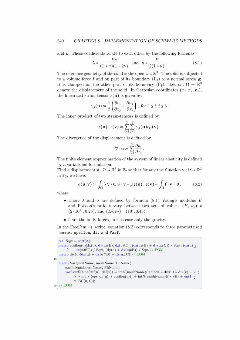
240 CHAPTER 8. IMPLEMENTATION OF SCHWARZ METHODS
and µ. These coefficients relate to each other by the following formulas:
λ = Eν
(1 + ν)(1 − 2ν) and µ = E
2(1 + ν) . (8.1)
The reference geometry of the solid is the open Ω ⊂ R3. The solid is subjectedto a volume force f and on part of its boundary (Γ3) to a normal stress g.It is clamped on the other part of its boundary (Γ1). Let u ∶ Ω → R3
denote the displacement of the solid. In Cartesian coordinates (x1, x2, x3),the linearized strain tensor ε(u) is given by:
εij(u) ∶= 1
2(∂ui∂xj
+ ∂uj∂xi
) , for 1 ≤ i, j ≤ 3 .
The inner product of two strain-tensors is defined by:
ε(u) ∶ ε(v) ∶=3
∑i=1
3
∑j=1
εij(u)εij(v) .
The divergence of the displacement is defined by
∇ ⋅ u ∶=3
∑i=1
∂ui∂xi
.
The finite element approximation of the system of linear elasticity is definedby a variational formulation:Find a displacement u ∶ Ω→ R3 in P2 so that for any test function v ∶ Ω→ R3
in P2, we have:
a(u,v) ∶= ∫Ωλ∇ ⋅ u ∇ ⋅ v + µε(u) ∶ ε(v) − ∫
Ωf ⋅ v = 0 , (8.2)
where
• where λ and ν are defined by formula (8.1) Young’s modulus Eand Poisson’s ratio ν vary between two sets of values, (E1, ν1) =(2 ⋅ 1011,0.25), and (E2, ν2) = (107,0.45).
• f are the body forces, in this case only the gravity.
In the FreeFem++ script, equation (8.2) corresponds to three parametrizedmacros: epsilon, div and Varf.
real Sqrt = sqrt(2.);macro epsilon(u)[dx(u), dy(u#B), dz(u#C), (dz(u#B) + dy(u#C)) / Sqrt, (dz(u) ⤸
Ç + dx(u#C)) / Sqrt, (dy(u) + dx(u#B)) / Sqrt]// EOMmacro div(u)(dx(u) + dy(u#B) + dz(u#C))// EOM
16
macro Varf(varfName, meshName, PhName)coefficients(meshName, PhName)varf varfName(def(u), def(v)) = intN(meshName)(lambda ∗ div(u) ∗ div(v) + 2. ⤸
Ç ∗ mu ∗ (epsilon(u)’ ∗ epsilon(v))) + intN(meshName)(f ∗ vB) + on(1, ⤸Ç BC(u, 0));
20 // EOM
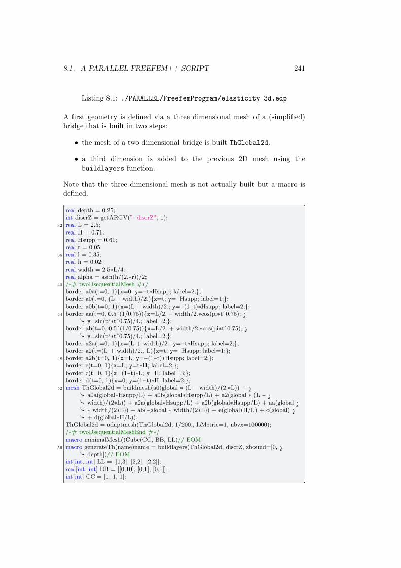
8.1. A PARALLEL FREEFEM++ SCRIPT 241
Listing 8.1: ./PARALLEL/FreefemProgram/elasticity-3d.edp
A first geometry is defined via a three dimensional mesh of a (simplified)bridge that is built in two steps:
• the mesh of a two dimensional bridge is built ThGlobal2d.
• a third dimension is added to the previous 2D mesh using thebuildlayers function.
Note that the three dimensional mesh is not actually built but a macro isdefined.
real depth = 0.25;int discrZ = getARGV(”−discrZ”, 1);
32 real L = 2.5;real H = 0.71;real Hsupp = 0.61;real r = 0.05;
36 real l = 0.35;real h = 0.02;real width = 2.5∗L/4.;real alpha = asin(h/(2.∗r))/2;
40 /∗# twoDsequentialMesh #∗/border a0a(t=0, 1)x=0; y=−t∗Hsupp; label=2;;border a0(t=0, (L − width)/2.)x=t; y=−Hsupp; label=1;;border a0b(t=0, 1)x=(L − width)/2.; y=−(1−t)∗Hsupp; label=2;;
44 border aa(t=0, 0.5ˆ(1/0.75))x=L/2. − width/2.∗cos(pi∗tˆ0.75); ⤸Ç y=sin(pi∗tˆ0.75)/4.; label=2;;
border ab(t=0, 0.5ˆ(1/0.75))x=L/2. + width/2.∗cos(pi∗tˆ0.75); ⤸Ç y=sin(pi∗tˆ0.75)/4.; label=2;;
border a2a(t=0, 1)x=(L + width)/2.; y=−t∗Hsupp; label=2;;border a2(t=(L + width)/2., L)x=t; y=−Hsupp; label=1;;
48 border a2b(t=0, 1)x=L; y=−(1−t)∗Hsupp; label=2;;border e(t=0, 1)x=L; y=t∗H; label=2;;border c(t=0, 1)x=(1−t)∗L; y=H; label=3;;border d(t=0, 1)x=0; y=(1−t)∗H; label=2;;
52 mesh ThGlobal2d = buildmesh(a0(global ∗ (L − width)/(2.∗L)) + ⤸Ç a0a(global∗Hsupp/L) + a0b(global∗Hsupp/L) + a2(global ∗ (L − ⤸Ç width)/(2∗L)) + a2a(global∗Hsupp/L) + a2b(global∗Hsupp/L) + aa(global ⤸Ç ∗ width/(2∗L)) + ab(−global ∗ width/(2∗L)) + e(global∗H/L) + c(global) ⤸Ç + d(global∗H/L));
ThGlobal2d = adaptmesh(ThGlobal2d, 1/200., IsMetric=1, nbvx=100000);/∗# twoDsequentialMeshEnd #∗/macro minimalMesh()Cube(CC, BB, LL)// EOM
56 macro generateTh(name)name = buildlayers(ThGlobal2d, discrZ, zbound=[0, ⤸Ç depth])// EOM
int[int, int] LL = [[1,3], [2,2], [2,2]];real[int, int] BB = [[0,10], [0,1], [0,1]];int[int] CC = [1, 1, 1];
242 CHAPTER 8. IMPLEMENTATION OF SCHWARZ METHODS
Listing 8.2: ./PARALLEL/FreefemProgram/elasticity-3d.edpThis geometry is partitioned and distributed among the MPI processes.
Figure 8.1: Partitioning into eight subdomains
From now on, all the tasks can be computed concurrently, meaning thateach MPI process is in charge of only one subdomain and variables are localto each process. Then a parallel mesh refinement is made by cutting eachtetrahedra into 8 tetrahedra. This corresponds to a mesh refinement factors equals to 2. Note also that at this point, the displacement field u isapproximated by P2 continuous piecewise quadratic functions.
func Pk = [P2, P2, P2];
build(generateTh, Th, ThBorder, ThOverlap, D, numberIntersection, ⤸Ç arrayIntersection, restrictionIntersection, Wh, Pk, mpiCommWorld, s)
75 ThGlobal2d = square(1, 1);
Listing 8.3: ./PARALLEL/FreefemProgram/elasticity-3d.edpThe Young and Poisson modulus are heterogeneous and the exterior forcesare constant.
Remark 8.1.1 In our numerical experiments, Poisson’s ratio being rela-tively far from the incompressible limit of 0.5, it is not necessary to switchto a mixed finite element formulation since there is no locking effect.

8.1. A PARALLEL FREEFEM++ SCRIPT 243
real f = −900000.;func real stripes(real a, real b, real paramA, real paramB)
int da = int(a ∗ 10);107 return (da == (int(da / 2) ∗ 2) ? paramB : paramA);
macro coefficients(meshName, PhName)111 fespace PhName(meshName, P0);
PhName Young = stripes(y, x, 2e11, 1e7);PhName poisson = stripes(y, x, 0.25, 0.45);PhName tmp = 1. + poisson;
115 PhName mu = Young / (2. ∗ tmp);PhName lambda = Young ∗ poisson / (tmp ∗ (1. − 2. ∗ poisson));// EOM
Listing 8.4: ./PARALLEL/FreefemProgram/elasticity-3d.edp
8.1.2 Native DDM solvers and PETSc Interface
At this point, the physics, the geometry and the discretization of the threedimensional elasticity problem have been given in the script. In order tofind the finite element approximation of the displacement field, we haveto solve the corresponding global algebraic system which is actually neverassembled. Its distributed storage among the processes depends on whetherwe use native FreeFem++ solvers or other solvers via the PETSc interface.The native FreeFem++ solvers are:
• a parallel GMRES solver which is the default parallel solver inFreeFem++,
• a one-level Schwarz method, either ASM or RAS,
• the two-level Schwarz method with a GenEO coarse space, § 7.
They are implemented inside HPDDM, a C++ framework for high-performance domain decomposition methods, available at the followingURL: https://github.com/hpddm/hpddm. Its interface with FreeFem++also include substructuring methods, like the FETI and BDD methods, asdescribed § 6. The solvers interfaced with PETSc are:
• the PETSc parallel GMRES solver,
• the multi frontal parallel solver MUMPS [5],
• GAMG: an algebraic multigrid solver [2].

244 CHAPTER 8. IMPLEMENTATION OF SCHWARZ METHODS
solver = getARGV(”−solver”, 0);if(solver == 0)
82 if(mpirank == 0)
cout << ”What kind of solver would you like to use ?” << endl;cout << ” [1] PETSc GMRES” << endl;
86 cout << ” [2] GAMG” << endl;cout << ” [3] MUMPS” << endl;cout << ” [10] ASM” << endl;cout << ” [11] RAS” << endl;
90 cout << ” [12] Schwarz GenEO” << endl;cout << ” [13] GMRES” << endl;cout << ”Please type in a number: ”;cin >> solver;
94 if(solver != 1 && solver != 2 && solver != 3 && solver != 4 && solver ⤸Ç != 10 && solver != 11 && solver != 12)
cout << ”Wrong choice, using GMRES instead !” << endl;solver = 10;
98
broadcast(processor(0), solver);
Listing 8.5: ./PARALLEL/FreefemProgram/elasticity-3d.edp
FreeFem++ interface If the native FreeFem++ solvers are used, thelocal stiffness matrices are assembled concurrently:
assemble(A, rhs, Wh, Th, ThBorder, Varf)
Listing 8.6: ./PARALLEL/FreefemProgram/elasticity-3d.edpThe local operator is attached to a distributed structure dschwarz whichis a FreeFem++ type. If necessary, the GenEO coarse space is built:
matrix N;if(mpisize > 1 && solver == 12)
166 int[int] parm(1);parm(0) = getARGV(”−nu”, 20);EVproblem(vPbNoPen, Th, Ph)matrix noPen = vPbNoPen(Wh, Wh, solver = CG);
170 attachCoarseOperator(mpiCommWorld, Aglob, A = noPen, /∗threshold = 2. ⤸Ç ∗ h[].max / diam,∗/ parameters = parm);
Listing 8.7: ./PARALLEL/FreefemProgram/elasticity-3d.edpThe distributed linear system is solved by a call that includes addi-tional command line arguments that are automatically passed to thesolvers.

8.1. A PARALLEL FREEFEM++ SCRIPT 245
DDM(Aglob, u[], rhs, dim = getARGV(”−gmres restart”, 60), iter = ⤸Ç getARGV(”−iter”, 100), eps = getARGV(”−eps”, 1e−8), solver = ⤸Ç solver − 9);
Listing 8.8: ./PARALLEL/FreefemProgram/elasticity-3d.edp
PETSc interface If the PETSc interface is used, the local stiffness matrixK ∶= Aii ∶= RiARTi and the local load vector rhs are built concurrently fromthe variational forms for all subdomains 1 ≤ i ≤ N .
124 Varf(vPb, Th, Ph)matrix A = vPb(Wh, Wh);rhs = vPb(0, Wh);dmatrix Mat(A, arrayIntersection, restrictionIntersection, D, bs = 3);
Listing 8.9: ./PARALLEL/FreefemProgram/elasticity-3d.edpdmatrix is a FreeFem++ type.If an algebraic multigrid method is used via the PETSc interface, the nearnull space must be provided in order to enhance the convergence, see e.g.[109]. For an elasticity problem, it is made of the rigid body motions whichare three translations and three rotations, here along the axis.
Wh[int] def(Rb)(6);[Rb[0], RbB[0], RbC[0]] = [ 1, 0, 0];[Rb[1], RbB[1], RbC[1]] = [ 0, 1, 0];
135 [Rb[2], RbB[2], RbC[2]] = [ 0, 0, 1];[Rb[3], RbB[3], RbC[3]] = [ y, −x, 0];[Rb[4], RbB[4], RbC[4]] = [−z, 0, x];[Rb[5], RbB[5], RbC[5]] = [ 0, z, −y];
Listing 8.10: ./PARALLEL/FreefemProgram/elasticity-3d.edpEventually, the solver may be called by passing command line parametersto PETSc:
141 set(Mat, sparams = ”−pc type gamg −ksp type gmres −pc gamg threshold ⤸Ç 0.05 −ksp monitor”, nearnullspace = Rb);
else if(solver == 3)
set(Mat, sparams = ”−pc type lu −pc factor mat solver package mumps ⤸Ç −mat mumps icntl 7 2 −ksp monitor”);
145 mpiBarrier(mpiCommWorld);timing = mpiWtime();
u[] = Mat−1 ∗ rhs;
Listing 8.11: ./PARALLEL/FreefemProgram/elasticity-3d.edp
246 CHAPTER 8. IMPLEMENTATION OF SCHWARZ METHODS
8.1.3 Validation of the computation
The true residual is computed by first performing a parallel matrix vec-tor product either via matrix Mat that is interfaced with the PETSc inter-face
res = Mat ∗ u[];
Listing 8.12: ./PARALLEL/FreefemProgram/elasticity-3d.edpor via the matrix Aglob in the “native” FreeFem++ Schwarz for-mat.
res = Aglob ∗ u[];
Listing 8.13: ./PARALLEL/FreefemProgram/elasticity-3d.edpOnce the linear system is solved and the residual is computed, the sequelof the program does not depend on whether a FreeFem++ or a PETScinterface was used. The residual is subtracted from the distributed right-hand side rhs and distributed scalar product are performed based onLemma 8.3.1
182 res −= rhs;real rhsnorm = dscalprod(D, rhs, rhs);real dist = dscalprod(D, res, res);if(mpirank == 0)
186 cout << ” −−− normalized Lˆ2 norm of the true residual: ” << sqrt(dist / ⤸Ç rhsnorm) << endl;
Listing 8.14: ./PARALLEL/FreefemProgram/elasticity-3d.edpThe three dimensional solution can be visualized by the plot com-mand.
193 plotMPI(Th, u, ”Global solution”, Pk, def, 3, 1);meshN ThMoved = movemesh3(Th, transfo = [x + u, y + uB, z + uC]);plotMPI(ThMoved, u, ”Moved mesh”, Pk, def, 3, 1);
Listing 8.15: ./PARALLEL/FreefemProgram/elasticity-3d.edp
Timings for the solvers are given in Section 8.2.
8.1.4 Parallel Script
For sake of completeness, the full script is given here, split into fivepieces.

8.1. A PARALLEL FREEFEM++ SCRIPT 247
macro K()real// EOMmacro def()def3// EOMmacro init()init3// EOM
5 macro BC()BC3// EOMmacro meshN()mesh3// EOMmacro intN()int3d// EOMmacro measureN()volume// EOM
9 macro bbN()bb3// EOMinclude ”Schwarz/macro.idp”
/∗# problemPhysics #∗/13 real Sqrt = sqrt(2.);
macro epsilon(u)[dx(u), dy(u#B), dz(u#C), (dz(u#B) + dy(u#C)) / Sqrt, (dz(u) ⤸Ç + dx(u#C)) / Sqrt, (dy(u) + dx(u#B)) / Sqrt]// EOM
macro div(u)(dx(u) + dy(u#B) + dz(u#C))// EOM
17 macro Varf(varfName, meshName, PhName)coefficients(meshName, PhName)varf varfName(def(u), def(v)) = intN(meshName)(lambda ∗ div(u) ∗ div(v) + 2. ⤸
Ç ∗ mu ∗ (epsilon(u)’ ∗ epsilon(v))) + intN(meshName)(f ∗ vB) + on(1, ⤸Ç BC(u, 0));
// EOM21 /∗# problemPhysicsEnd #∗/
/∗# vfGENEO #∗/macro EVproblem(varfName, meshName, PhName)
coefficients(meshName, PhName)25 varf varfName(def(u), def(v)) = intN(meshName)(lambda ∗ div(u) ∗ div(v) + 2. ⤸
Ç ∗ mu ∗ (epsilon(u)’ ∗ epsilon(v))) + on(1, BC(u, 0));// EOM/∗# vfGENEOEnd #∗/
29 /∗# sequentialMesh #∗/real depth = 0.25;int discrZ = getARGV(”−discrZ”, 1);real L = 2.5;
33 real H = 0.71;real Hsupp = 0.61;real r = 0.05;real l = 0.35;
37 real h = 0.02;real width = 2.5∗L/4.;real alpha = asin(h/(2.∗r))/2;
Listing 8.16: ./PARALLEL/FreefemProgram/elasticity-3d.edp

248 CHAPTER 8. IMPLEMENTATION OF SCHWARZ METHODS
border a0a(t=0, 1)x=0; y=−t∗Hsupp; label=2;;border a0(t=0, (L − width)/2.)x=t; y=−Hsupp; label=1;;border a0b(t=0, 1)x=(L − width)/2.; y=−(1−t)∗Hsupp; label=2;;
44 border aa(t=0, 0.5ˆ(1/0.75))x=L/2. − width/2.∗cos(pi∗tˆ0.75); ⤸Ç y=sin(pi∗tˆ0.75)/4.; label=2;;
border ab(t=0, 0.5ˆ(1/0.75))x=L/2. + width/2.∗cos(pi∗tˆ0.75); ⤸Ç y=sin(pi∗tˆ0.75)/4.; label=2;;
border a2a(t=0, 1)x=(L + width)/2.; y=−t∗Hsupp; label=2;;border a2(t=(L + width)/2., L)x=t; y=−Hsupp; label=1;;
48 border a2b(t=0, 1)x=L; y=−(1−t)∗Hsupp; label=2;;border e(t=0, 1)x=L; y=t∗H; label=2;;border c(t=0, 1)x=(1−t)∗L; y=H; label=3;;border d(t=0, 1)x=0; y=(1−t)∗H; label=2;;
52 mesh ThGlobal2d = buildmesh(a0(global ∗ (L − width)/(2.∗L)) + ⤸Ç a0a(global∗Hsupp/L) + a0b(global∗Hsupp/L) + a2(global ∗ (L − ⤸Ç width)/(2∗L)) + a2a(global∗Hsupp/L) + a2b(global∗Hsupp/L) + aa(global ⤸Ç ∗ width/(2∗L)) + ab(−global ∗ width/(2∗L)) + e(global∗H/L) + c(global) ⤸Ç + d(global∗H/L));
ThGlobal2d = adaptmesh(ThGlobal2d, 1/200., IsMetric=1, nbvx=100000);/∗# twoDsequentialMeshEnd #∗/macro minimalMesh()Cube(CC, BB, LL)// EOM
56 macro generateTh(name)name = buildlayers(ThGlobal2d, discrZ, zbound=[0, ⤸Ç depth])// EOM
int[int, int] LL = [[1,3], [2,2], [2,2]];real[int, int] BB = [[0,10], [0,1], [0,1]];int[int] CC = [1, 1, 1];
60 /∗# sequentialMeshEnd #∗/
include ”Schwarz/additional macro.idp”
64 int overlap = getARGV(”−overlap”, 1);
if(mpirank == 0) cout << ” −−− ” << mpirank << ”/” << mpisize;
68 cout << ” − input parameters: global size = ” << global << ” − refinement ⤸Ç factor = ” << s << ” − precision = ” << getARGV(”−eps”, 1e−8) << ⤸Ç ” − overlap = ” << overlap << ” − with partitioner? = ” << ⤸Ç partitioner << endl;
/∗# parallelMesh #∗/72 func Pk = [P2, P2, P2];
build(generateTh, Th, ThBorder, ThOverlap, D, numberIntersection, ⤸Ç arrayIntersection, restrictionIntersection, Wh, Pk, mpiCommWorld, s)
ThGlobal2d = square(1, 1);
Listing 8.17: ./PARALLEL/FreefemProgram/elasticity-3d.edp

8.1. A PARALLEL FREEFEM++ SCRIPT 249
Wh def(u);/∗# chooseSolver #∗/
80 solver = getARGV(”−solver”, 0);if(solver == 0)
if(mpirank == 0) 84 cout << ”What kind of solver would you like to use ?” << endl;
cout << ” [1] PETSc GMRES” << endl;cout << ” [2] GAMG” << endl;cout << ” [3] MUMPS” << endl;
88 cout << ” [10] ASM” << endl;cout << ” [11] RAS” << endl;cout << ” [12] Schwarz GenEO” << endl;cout << ” [13] GMRES” << endl;
92 cout << ”Please type in a number: ”;cin >> solver;if(solver != 1 && solver != 2 && solver != 3 && solver != 4 && solver ⤸
Ç != 10 && solver != 11 && solver != 12) cout << ”Wrong choice, using GMRES instead !” << endl;
96 solver = 10;
100 broadcast(processor(0), solver);/∗# chooseSolverEnd #∗/
/∗# physicalParameters #∗/104 real f = −900000.;
func real stripes(real a, real b, real paramA, real paramB) int da = int(a ∗ 10);return (da == (int(da / 2) ∗ 2) ? paramB : paramA);
108
macro coefficients(meshName, PhName)fespace PhName(meshName, P0);
112 PhName Young = stripes(y, x, 2e11, 1e7);PhName poisson = stripes(y, x, 0.25, 0.45);PhName tmp = 1. + poisson;PhName mu = Young / (2. ∗ tmp);
116 PhName lambda = Young ∗ poisson / (tmp ∗ (1. − 2. ∗ poisson));// EOM
Listing 8.18: ./PARALLEL/FreefemProgram/elasticity-3d.edp

250 CHAPTER 8. IMPLEMENTATION OF SCHWARZ METHODS
real[int] res(Wh.ndof);120 real[int] rhs(Wh.ndof);
if(solver == 1 || solver == 2 || solver == 3) /∗# StiffnessRhsMatrix #∗/
124 Varf(vPb, Th, Ph)matrix A = vPb(Wh, Wh);rhs = vPb(0, Wh);dmatrix Mat(A, arrayIntersection, restrictionIntersection, D, bs = 3);
128 /∗# StiffnessRhsMatrixEnd #∗/// sparams will override command line arguments !if(solver == 2)
/∗# rigidBodyMotion #∗/132 Wh[int] def(Rb)(6);
[Rb[0], RbB[0], RbC[0]] = [ 1, 0, 0];[Rb[1], RbB[1], RbC[1]] = [ 0, 1, 0];[Rb[2], RbB[2], RbC[2]] = [ 0, 0, 1];
136 [Rb[3], RbB[3], RbC[3]] = [ y, −x, 0];[Rb[4], RbB[4], RbC[4]] = [−z, 0, x];[Rb[5], RbB[5], RbC[5]] = [ 0, z, −y];
/∗# rigidBodyMotionEnd #∗/140 /∗# SolverPETSc #∗/
set(Mat, sparams = ”−pc type gamg −ksp type gmres −pc gamg threshold ⤸Ç 0.05 −ksp monitor”, nearnullspace = Rb);
else if(solver == 3)
144 set(Mat, sparams = ”−pc type lu −pc factor mat solver package mumps ⤸Ç −mat mumps icntl 7 2 −ksp monitor”);
mpiBarrier(mpiCommWorld);timing = mpiWtime();
u[] = Mat−1 ∗ rhs;148 /∗# SolverPETScEnd #∗/
timing = mpiWtime() − timing;/∗# matrixVectorPETSc #∗/
res = Mat ∗ u[];152 /∗# matrixVectorPETScEnd #∗/
else
/∗# localMatrix #∗/156 assemble(A, rhs, Wh, Th, ThBorder, Varf)
Listing 8.19: ./PARALLEL/FreefemProgram/elasticity-3d.edp
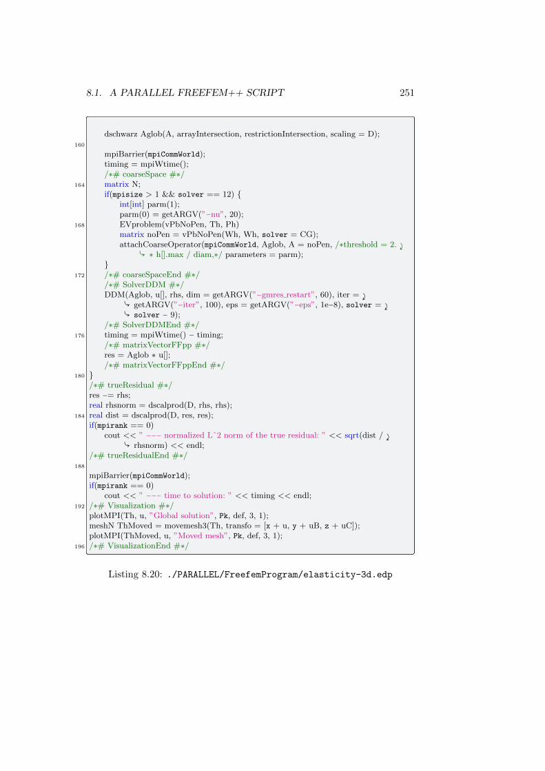
8.1. A PARALLEL FREEFEM++ SCRIPT 251
dschwarz Aglob(A, arrayIntersection, restrictionIntersection, scaling = D);160
mpiBarrier(mpiCommWorld);timing = mpiWtime();/∗# coarseSpace #∗/
164 matrix N;if(mpisize > 1 && solver == 12)
int[int] parm(1);parm(0) = getARGV(”−nu”, 20);
168 EVproblem(vPbNoPen, Th, Ph)matrix noPen = vPbNoPen(Wh, Wh, solver = CG);attachCoarseOperator(mpiCommWorld, Aglob, A = noPen, /∗threshold = 2. ⤸
Ç ∗ h[].max / diam,∗/ parameters = parm);
172 /∗# coarseSpaceEnd #∗//∗# SolverDDM #∗/DDM(Aglob, u[], rhs, dim = getARGV(”−gmres restart”, 60), iter = ⤸
Ç getARGV(”−iter”, 100), eps = getARGV(”−eps”, 1e−8), solver = ⤸Ç solver − 9);
/∗# SolverDDMEnd #∗/176 timing = mpiWtime() − timing;
/∗# matrixVectorFFpp #∗/res = Aglob ∗ u[];/∗# matrixVectorFFppEnd #∗/
180 /∗# trueResidual #∗/res −= rhs;real rhsnorm = dscalprod(D, rhs, rhs);
184 real dist = dscalprod(D, res, res);if(mpirank == 0)
cout << ” −−− normalized Lˆ2 norm of the true residual: ” << sqrt(dist / ⤸Ç rhsnorm) << endl;
/∗# trueResidualEnd #∗/188
mpiBarrier(mpiCommWorld);if(mpirank == 0)
cout << ” −−− time to solution: ” << timing << endl;192 /∗# Visualization #∗/
plotMPI(Th, u, ”Global solution”, Pk, def, 3, 1);meshN ThMoved = movemesh3(Th, transfo = [x + u, y + uB, z + uC]);plotMPI(ThMoved, u, ”Moved mesh”, Pk, def, 3, 1);
196 /∗# VisualizationEnd #∗/
Listing 8.20: ./PARALLEL/FreefemProgram/elasticity-3d.edp
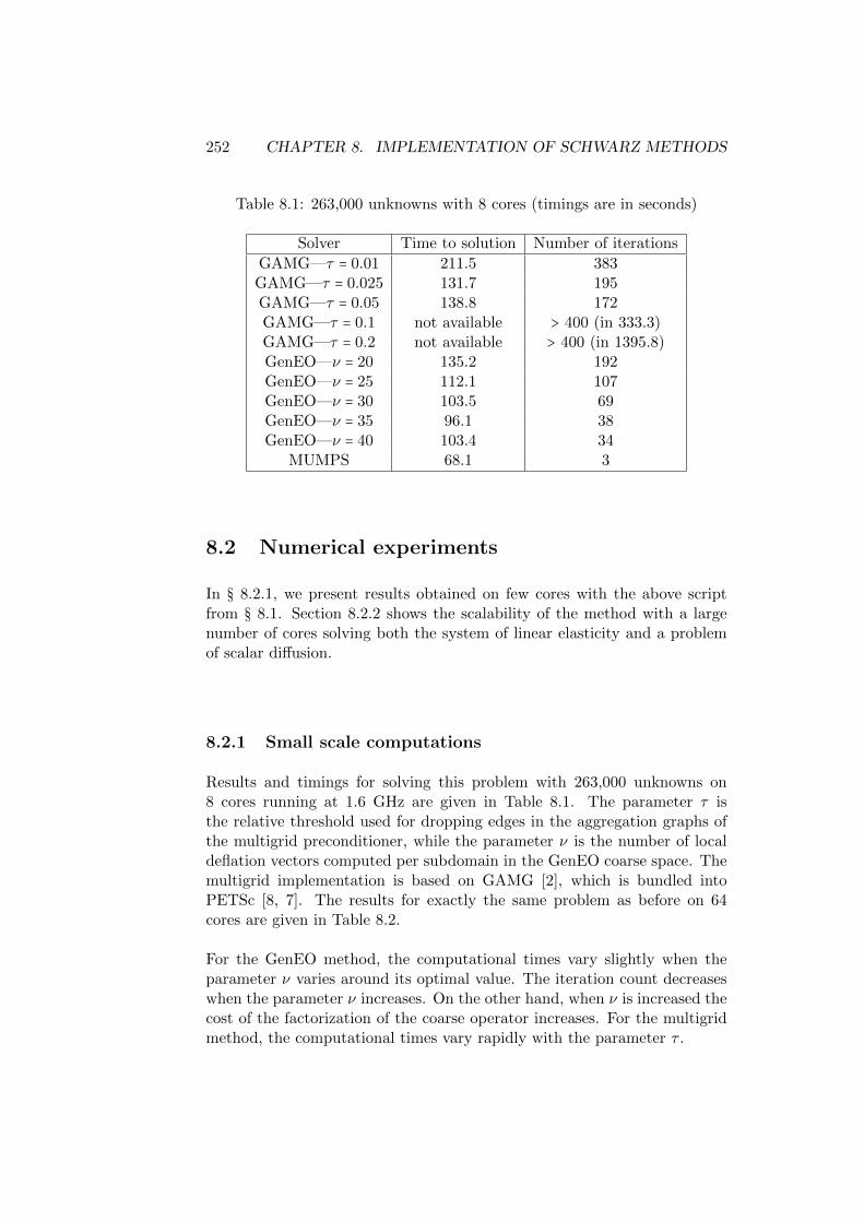
252 CHAPTER 8. IMPLEMENTATION OF SCHWARZ METHODS
Table 8.1: 263,000 unknowns with 8 cores (timings are in seconds)
Solver Time to solution Number of iterations
GAMG—τ = 0.01 211.5 383GAMG—τ = 0.025 131.7 195GAMG—τ = 0.05 138.8 172GAMG—τ = 0.1 not available > 400 (in 333.3)GAMG—τ = 0.2 not available > 400 (in 1395.8)GenEO—ν = 20 135.2 192GenEO—ν = 25 112.1 107GenEO—ν = 30 103.5 69GenEO—ν = 35 96.1 38GenEO—ν = 40 103.4 34
MUMPS 68.1 3
8.2 Numerical experiments
In § 8.2.1, we present results obtained on few cores with the above scriptfrom § 8.1. Section 8.2.2 shows the scalability of the method with a largenumber of cores solving both the system of linear elasticity and a problemof scalar diffusion.
8.2.1 Small scale computations
Results and timings for solving this problem with 263,000 unknowns on8 cores running at 1.6 GHz are given in Table 8.1. The parameter τ isthe relative threshold used for dropping edges in the aggregation graphs ofthe multigrid preconditioner, while the parameter ν is the number of localdeflation vectors computed per subdomain in the GenEO coarse space. Themultigrid implementation is based on GAMG [2], which is bundled intoPETSc [8, 7]. The results for exactly the same problem as before on 64cores are given in Table 8.2.
For the GenEO method, the computational times vary slightly when theparameter ν varies around its optimal value. The iteration count decreaseswhen the parameter ν increases. On the other hand, when ν is increased thecost of the factorization of the coarse operator increases. For the multigridmethod, the computational times vary rapidly with the parameter τ .
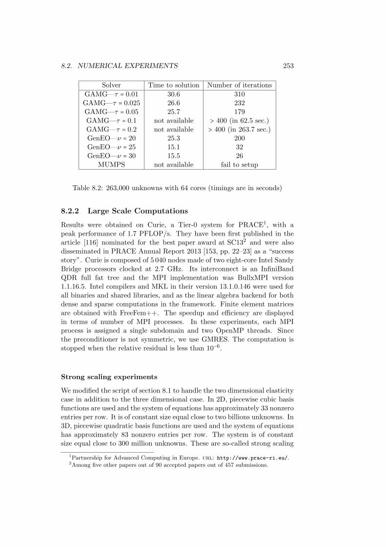
8.2. NUMERICAL EXPERIMENTS 253
Solver Time to solution Number of iterations
GAMG—τ = 0.01 30.6 310GAMG—τ = 0.025 26.6 232GAMG—τ = 0.05 25.7 179GAMG—τ = 0.1 not available > 400 (in 62.5 sec.)GAMG—τ = 0.2 not available > 400 (in 263.7 sec.)GenEO—ν = 20 25.3 200GenEO—ν = 25 15.1 32GenEO—ν = 30 15.5 26
MUMPS not available fail to setup
Table 8.2: 263,000 unknowns with 64 cores (timings are in seconds)
8.2.2 Large Scale Computations
Results were obtained on Curie, a Tier-0 system for PRACE1, with apeak performance of 1.7 PFLOP/s. They have been first published in thearticle [116] nominated for the best paper award at SC132 and were alsodisseminated in PRACE Annual Report 2013 [153, pp. 22–23] as a “successstory”. Curie is composed of 5 040 nodes made of two eight-core Intel SandyBridge processors clocked at 2.7 GHz. Its interconnect is an InfiniBandQDR full fat tree and the MPI implementation was BullxMPI version1.1.16.5. Intel compilers and MKL in their version 13.1.0.146 were used forall binaries and shared libraries, and as the linear algebra backend for bothdense and sparse computations in the framework. Finite element matricesare obtained with FreeFem++. The speedup and efficiency are displayedin terms of number of MPI processes. In these experiments, each MPIprocess is assigned a single subdomain and two OpenMP threads. Sincethe preconditioner is not symmetric, we use GMRES. The computation isstopped when the relative residual is less than 10−6.
Strong scaling experiments
We modified the script of section 8.1 to handle the two dimensional elasticitycase in addition to the three dimensional case. In 2D, piecewise cubic basisfunctions are used and the system of equations has approximately 33 nonzeroentries per row. It is of constant size equal close to two billions unknowns. In3D, piecewise quadratic basis functions are used and the system of equationshas approximately 83 nonzero entries per row. The system is of constantsize equal close to 300 million unknowns. These are so-called strong scaling
1Partnership for Advanced Computing in Europe. url: http://www.prace-ri.eu/.2Among five other papers out of 90 accepted papers out of 457 submissions.
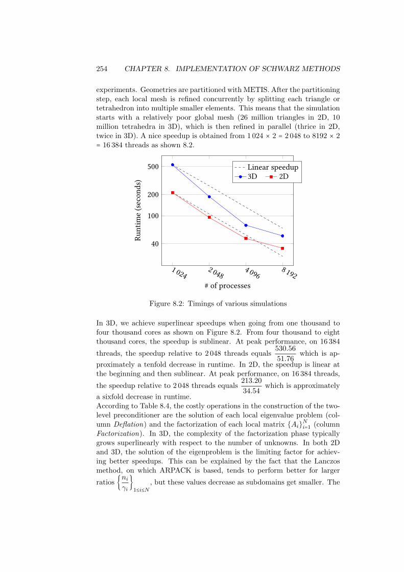
254 CHAPTER 8. IMPLEMENTATION OF SCHWARZ METHODS
experiments. Geometries are partitioned with METIS. After the partitioningstep, each local mesh is refined concurrently by splitting each triangle ortetrahedron into multiple smaller elements. This means that the simulationstarts with a relatively poor global mesh (26 million triangles in 2D, 10million tetrahedra in 3D), which is then refined in parallel (thrice in 2D,twice in 3D). A nice speedup is obtained from 1 024 × 2 = 2 048 to 8192 × 2= 16 384 threads as shown 8.2.
1 0242 048
4 0968 192
40
100
200
500
# of processes
Runtim
e(secon
ds)
Linear speedup3D 2D
Figure 8.2: Timings of various simulations
In 3D, we achieve superlinear speedups when going from one thousand tofour thousand cores as shown on Figure 8.2. From four thousand to eightthousand cores, the speedup is sublinear. At peak performance, on 16 384
threads, the speedup relative to 2 048 threads equals530.56
51.76which is ap-
proximately a tenfold decrease in runtime. In 2D, the speedup is linear atthe beginning and then sublinear. At peak performance, on 16 384 threads,
the speedup relative to 2 048 threads equals213.20
34.54which is approximately
a sixfold decrease in runtime.According to Table 8.4, the costly operations in the construction of the two-level preconditioner are the solution of each local eigenvalue problem (col-umn Deflation) and the factorization of each local matrix AiNi=1 (columnFactorization). In 3D, the complexity of the factorization phase typicallygrows superlinearly with respect to the number of unknowns. In both 2Dand 3D, the solution of the eigenproblem is the limiting factor for achiev-ing better speedups. This can be explained by the fact that the Lanczosmethod, on which ARPACK is based, tends to perform better for larger
ratios niγi
1≤i≤N
, but these values decrease as subdomains get smaller. The
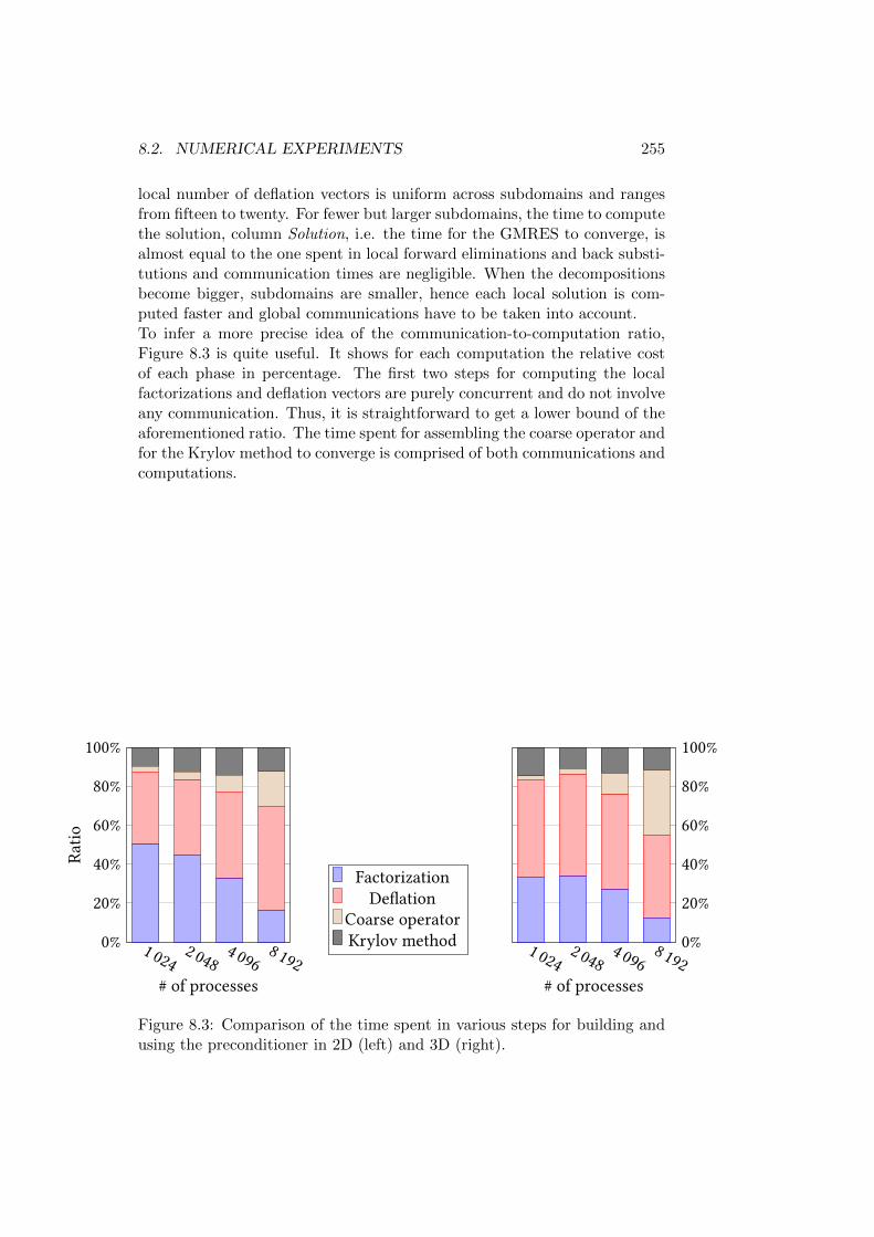
8.2. NUMERICAL EXPERIMENTS 255
local number of deflation vectors is uniform across subdomains and rangesfrom fifteen to twenty. For fewer but larger subdomains, the time to computethe solution, column Solution, i.e. the time for the GMRES to converge, isalmost equal to the one spent in local forward eliminations and back substi-tutions and communication times are negligible. When the decompositionsbecome bigger, subdomains are smaller, hence each local solution is com-puted faster and global communications have to be taken into account.To infer a more precise idea of the communication-to-computation ratio,Figure 8.3 is quite useful. It shows for each computation the relative costof each phase in percentage. The first two steps for computing the localfactorizations and deflation vectors are purely concurrent and do not involveany communication. Thus, it is straightforward to get a lower bound of theaforementioned ratio. The time spent for assembling the coarse operator andfor the Krylov method to converge is comprised of both communications andcomputations.
1 0242 048
4 0968 192
0%
20%
40%
60%
80%
100%
# of processes
Ratio
1 0242 048
4 0968 192
0%
20%
40%
60%
80%
100%
# of processes
FactorizationDeflation
Coarse operatorKrylov method
Figure 8.3: Comparison of the time spent in various steps for building andusing the preconditioner in 2D (left) and 3D (right).
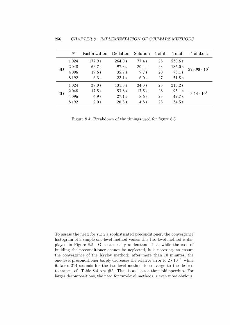
256 CHAPTER 8. IMPLEMENTATION OF SCHWARZ METHODS
N Factorization Deflation Solution # of it. Total # of d.o.f.
3D
1 024 177.9 s 264.0 s 77.4 s 28 530.6 s
293.98 · 1062 048 62.7 s 97.3 s 20.4 s 23 186.0 s4 096 19.6 s 35.7 s 9.7 s 20 73.1 s8 192 6.3 s 22.1 s 6.0 s 27 51.8 s
2D
1 024 37.0 s 131.8 s 34.3 s 28 213.2 s
2.14 · 1092 048 17.5 s 53.8 s 17.5 s 28 95.1 s4 096 6.9 s 27.1 s 8.6 s 23 47.7 s8 192 2.0 s 20.8 s 4.8 s 23 34.5 s
Figure 8.4: Breakdown of the timings used for figure 8.3.
To assess the need for such a sophisticated preconditioner, the convergencehistogram of a simple one-level method versus this two-level method is dis-played in Figure 8.5. One can easily understand that, while the cost ofbuilding the preconditioner cannot be neglected, it is necessary to ensurethe convergence of the Krylov method: after more than 10 minutes, theone-level preconditioner barely decreases the relative error to 2×10⁻⁵, whileit takes 214 seconds for the two-level method to converge to the desiredtolerance, cf. Table 8.4 row #5. That is at least a threefold speedup. Forlarger decompositions, the need for two-level methods is even more obvious.

8.2. NUMERICAL EXPERIMENTS 257
0 100 200 300 400
10−6
10−5
10−4
10−3
10−2
# of iterations
Relativ
eresidu
alerror
M−1RAS eq. (1.15)
P−1A-DEF1 eq. (1.19a)
Figure 8.5:Convergence of the restarted GMRES(40) for a 2D problemof linear elasticity using 1 024 subdomains. Timings for thesetup and solution phases using P−1
A-DEF1 are available in 8.4,using M−1
RAS, the convergence is not reached after 10 minutes.
Weak scaling experiments
Moving on to the weak scaling properties, see Definition 4.1.2, the problemnow being solved is a scalar equation of diffusivity
−∇ ⋅ (κ∇u) = 1 in Ωu = 0 on [0; 1] × 0 . (8.3)
with highly heterogeneous coefficients. Parameter κ varies from 1 to 3 ⋅ 106
as displayed in Figure 8.6. The partitioned domain is Ω = [0; 1]d (d = 2 or3) with piecewise quartic basis functions in 2D yielding linear systems withapproximately 23 nonzero entries per row, and piecewise quadratic basisfunctions in 3D yielding linear systems with approximately 27 nonzeroentries per row. After using Green’s formula, its variational formulation is,for all test functions v ∈H1
0(Ω):
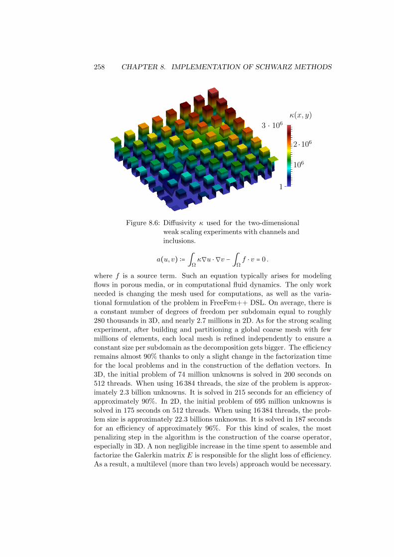
258 CHAPTER 8. IMPLEMENTATION OF SCHWARZ METHODS
κ(x, y)
3 · 106
2 ·106
106
1
Figure 8.6: Diffusivity κ used for the two-dimensionalweak scaling experiments with channels andinclusions.
a(u, v) ∶= ∫Ωκ∇u ⋅ ∇v − ∫
Ωf ⋅ v = 0 .
where f is a source term. Such an equation typically arises for modelingflows in porous media, or in computational fluid dynamics. The only workneeded is changing the mesh used for computations, as well as the varia-tional formulation of the problem in FreeFem++ DSL. On average, there isa constant number of degrees of freedom per subdomain equal to roughly280 thousands in 3D, and nearly 2.7 millions in 2D. As for the strong scalingexperiment, after building and partitioning a global coarse mesh with fewmillions of elements, each local mesh is refined independently to ensure aconstant size per subdomain as the decomposition gets bigger. The efficiencyremains almost 90% thanks to only a slight change in the factorization timefor the local problems and in the construction of the deflation vectors. In3D, the initial problem of 74 million unknowns is solved in 200 seconds on512 threads. When using 16 384 threads, the size of the problem is approx-imately 2.3 billion unknowns. It is solved in 215 seconds for an efficiency ofapproximately 90%. In 2D, the initial problem of 695 million unknowns issolved in 175 seconds on 512 threads. When using 16 384 threads, the prob-lem size is approximately 22.3 billions unknowns. It is solved in 187 secondsfor an efficiency of approximately 96%. For this kind of scales, the mostpenalizing step in the algorithm is the construction of the coarse operator,especially in 3D. A non negligible increase in the time spent to assemble andfactorize the Galerkin matrix E is responsible for the slight loss of efficiency.As a result, a multilevel (more than two levels) approach would be necessary.

8.3. FREEFEM++ ALGEBRAIC FORMULATION 259
8.3 FreeFem++ Algebraic Formulation
We present here the way we compute a global matrix vector product orthe action of a global one-level preconditioner, using only their local com-ponents plus point-to-point (between a pair of processes) communications.The special feature of this implementation is that no global numbering ofthe unknowns is needed. This is the way domain decomposition methodshave been implemented in FreeFem++.Recall that the set of indices N is decomposed into N sets (Ni)1≤i≤N . AMPI-process is attached to each subset. Let n ∶= #N be the number of de-grees of freedom of the global finite element space. A global vector U ∈ Rnis stored in a distributed way. Each process i , 1 ≤ i ≤ N , stores the localvector Ui ∶= RiU ∈ R#Ni where Ri is the restriction operator introducedin chapter 1 Definition 1.3.1. A total storage of ∑Ni=1 #Ni scalars must beallocated, which is larger than the size n of the original system. The extracost in memory is not a problem since it is distributed among the N MPIprocesses. The unknowns in the intersection of two subsets of degrees offreedom are duplicated. It is important to ensure that the result (vi)1≤i≤N
of all linear algebra operators applied to this representation will preserve itscoherence, that is the duplicated degrees of freedom share the same valuesacross the subdomains Ni, 1 ≤ i ≤ N :
Definition 8.3.1 A sequence of local vectors (Vi)1≤i≤N ∈ ΠNi=1R#Ni is co-
herent if there exists a vector V ∈ Rn such that for all 1 ≤ i ≤ N , we have:
Vi = RiV .
Another equivalent definition could have been that for all 1 ≤ i, j ≤ N , wehave:
RTj RjRTi Ui = RTi RiRTj Uj .
We have to define basic linear algebra operations based on this distributedstorage and to ensure that all linear algebra operations are performed sothat the coherence is enforced, up to round-off errors.We start with the scalar product of two distributed vectors:
Lemma 8.3.1 Let U,V ∈ Rn. We have the following formula for theirscalar product (U,V):
(U,V) =N
∑i=1
(RiU,DiRiV) .
Proof Using the partition of unity (1.25)
Id =N
∑i=1
RTi DiRi ,
260 CHAPTER 8. IMPLEMENTATION OF SCHWARZ METHODS
we have:
(U,V) = (U,N
∑i=1
RTi DiRiV) =N
∑i=1
(RiU,DiRiV)
=N
∑i=1
(Ui,DiVi) .
Local scalar products are performed concurrently. Thus, the implemen-tation is parallel except for the sum which corresponds to a MPI Reduce
call across the N MPI processes. Note also that the implementation relieson the knowledge of a partition of unity so that the FreeFem++ syntax isdscalprod(D,u,v).
A axpy procedure y ← αx + y for x, y ∈ Rn and α ∈ R is easily implementedconcurrently for distributed vectors in the form:
yi ← αxi + yi ,∀1 ≤ i ≤ N .
The matrix-vector product is more intricate. Let A ∈ Rn×n be a matrix andlet U,V ∈ Rn be two global vectors. We want to compute V ∶= AU basedon a distributed storage of U in the form (Ui)1≤i≤N . Using the partition ofunity identity (1.25), we have for all 1 ≤ i ≤ N :
Vi ∶= RiAU =N
∑j=1
RiARTj DjRjU =
N
∑j=1
RiARTj DjUj .
If matrix A arises from a finite element discretization of a partial differentialequation as it is the case here when using FreeFem++, it is possible tosimplify the matrix-vector product. The sparsity pattern of matrix A followsthe one of the graph of the underlying mesh. Let k, l be two degrees offreedom associated to the basis functions φk and φl. If their supports havea zero measure intersection, then:
Akl = 0 .
We can take advantage of this sparsity pattern in the following way. A degreeof freedom k ∈ Nj is interior to Nj if for all i ≠ j and all l ∈ Ni ∖Nj , Akl = 0.Otherwise, it is said to be a boundary degree of freedom. If the overlap issufficient, it is possible to choose diagonal matrix Dj with zero entries forthe boundary degrees of freedom. Then all non zero rows of matrix ARTj Dj
have indices in Nj that is:
RiARTj Dj = RiRTj RjARTj Dj .

8.3. FREEFEM++ ALGEBRAIC FORMULATION 261
Moreover, for non neighboring subdomains indexed i and j, the interactionmatrix RiAR
Tj is zero. Denoting Oi the neighbors of a subdomain i
Oi ∶= j ∈ J1;NK ∶ j ≠ i and RiARTj ≠ 0 ,
we have:
Vi ∶= RiAU =N
∑j=1
RiARTj DjRjU = (RiARTi
´¹¹¹¹¹¹¹¹¹¸¹¹¹¹¹¹¹¹¹¹¶Aii
)DiUi+∑j∈Oi
RiRTj (RjARTj
´¹¹¹¹¹¹¹¹¹¹¸¹¹¹¹¹¹¹¹¹¹¹¶Ajj
)DjUj .
Matrix Ajj ∶= RjARTj is local to domain j. The matrix operation RiRTj
corresponds to copy data on the overlap from subdomain j to subdomain i.Therefore, the matrix vector product is computed in three steps:
• concurrent computing of (RjARTj )DjUj for all 1 ≤ j ≤ N ;
• neighbor to neighbor MPI-communications;
• concurrent sum of neighbor contributions.
More details can be found in the PhD manuscript of P. Jolivet written inEnglish [117].
Since we have basic linear algebra subroutines, we have all the necessaryingredients for solving concurrently the linear system Ax = b by a Krylovmethod such as CG (conjugate gradient) or GMRES. We now turn our at-tention to domain decomposition methods. The ASM preconditioner reads:
M−1ASM ∶=
N
∑j=1
RTj A−1jjRj .
Let R be a distributed residual so that each MPI process stores Rj ∶= Rj R,1 ≤ j ≤ N . We want to compute for each subdomain 1 ≤ i ≤ N the restrictionof the application of the ASM preconditioner to R:
RiM−1ASM R = Ri
N
∑j=1
RTj A−1jj Rj R = A−1
ii Ri + ∑j∈Oi
(RiRTj )A−1jj Rj .
This task is performed by first solving concurrently on all subdomains alinear system:
Ajj Zj = Rj ∀1 ≤ j ≤ n . (8.4)
Then data transfers between neighboring subdomains implement theRiR
Tj Zj formula. The contribution from neighboring subdomains are

262 CHAPTER 8. IMPLEMENTATION OF SCHWARZ METHODS
summed locally. This pattern is very similar to that of the matrix vec-tor product.The RAS preconditioner reads:
M−1RAS ∶=
N
∑j=1
RTj DjA−1jjRj .
Its application to a distributed residual r consists in computing:
RiM−1RAS R = Ri
N
∑j=1
RTj Dj A−1jj Rj R =DiA
−1ii Ri + ∑
j∈Oi
(RiRTj )Dj A−1jj Rj .
The only difference in the implementation of RAS compared to ASM lies inthe concurrent multiplication of the local solution to (8.4) by the partitionof unity matrix Dj before data transfer between neighboring subdomains.

8.3. FREEFEM++ ALGEBRAIC FORMULATION 263
256 512 1 0242 048
4 0968 192
0%
20%
40%
60%
80%
100%
# of processes
Efficiency
relativ
eto
256processes
3D2D
695
22 311
#of
d.o.f.—
inmillions
74
2 305
(a) Timings of various simulations
256 512 1 0242 048
4 0968 192
0
50
100
150
200
# of processes
Time(secon
ds)
2.1M d.o.f.sbdmn in 2D
256 512 1 0242 048
4 0968 192
0
100
200
# of processes
280k d.o.f.sbdmn in 3D
FactorizationDeflation
Coarse operatorKrylov method
(b) Comparison of the time spent in various steps for building and using the preconditioner

264 CHAPTER 8. IMPLEMENTATION OF SCHWARZ METHODS
N Factorization Deflation Solution # of it. Total # of d.o.f.
3D
256 64.2 s 117.7 s 15.8 s 13 200.6 s 74.6 · 106512 64.0 s 112.2 s 19.9 s 18 199.4 s 144.7 · 1061 024 63.2 s 118.6 s 16.2 s 14 202.4 s 288.8 · 1062 048 59.4 s 117.6 s 21.3 s 17 205.3 s 578.0 · 1064 096 58.1 s 110.7 s 27.9 s 20 207.5 s 1.2 · 1098 192 55.0 s 116.6 s 23.6 s 17 215.2 s 2.3 · 109
2D
256 29.4 s 111.3 s 25.7 s 29 175.8 s 696.0 · 106512 29.6 s 111.5 s 28.0 s 28 179.1 s 1.4 · 1091 024 29.4 s 112.2 s 33.6 s 28 185.2 s 2.8 · 1092 048 29.2 s 112.2 s 33.7 s 28 185.2 s 5.6 · 1094 096 29.8 s 113.7 s 31.0 s 26 185.4 s 11.2 · 1098 192 29.8 s 113.8 s 30.7 s 25 187.6 s 22.3 · 109
(c) Breakdown of the timings used for the figure on top
Figure 8.7: Weak scaling experiments.

Bibliography
[1] Yves Achdou, Patrick Le Tallec, Frederic Nataf, and MarinaVidrascu. A domain decomposition preconditioner for an advection-diffusion problem. Comput. methods appl. mech. engrg., 184:145–170,2000 (cited on page 155).
[2] M. Adams, H. Bayraktar, T. Keaveny, and P. Papadopoulos. Ul-trascalable implicit finite element analyses in solid mechanics withover a half a billion degrees of freedom. In Proceedings of the 2004acm/ieee conference on supercomputing. In SC04. IEEE ComputerSociety, 2004, 34:1–34:15 (cited on pages 243, 252).
[3] Hubert Alcin, Bruno Koobus, Olivier Allain, and Alain Dervieux.Efficiency and scalability of a two-level Schwarz algorithm for incom-pressible and compressible flows. Internat. j. numer. methods fluids,72(1):69–89, 2013. issn: 0271-2091. doi: 10.1002/fld.3733. url:http://dx.doi.org/10.1002/fld.3733 (cited on page 138).
[4] Ana Alonso-Rodriguez and Luca Gerardo-Giorda. New nonoverlap-ping domain decomposition methods for the harmonic Maxwell sys-tem. Siam j. sci. comput., 28(1):102–122, 2006 (cited on page 86).
[5] Patrick R. Amestoy, Iain S. Duff, Jean-Yves L’Excellent, and JackoKoster. A fully asynchronous multifrontal solver using distributed dy-namic scheduling. Siam j. matrix analysis and applications, 23(1):15–41, 2001 (cited on page 243).
[6] Xavier Antoine, Yassine Boubendir, and Christophe Geuzaine. Aquasi-optimal non-overlapping domain decomposition algorithm forthe Helmholtz equation. Journal of computational physic, 231(2):262–280, 2012 (cited on page 86).
[7] Satish Balay, Shrirang Abhyankar, Mark F. Adams, Jed Brown, PeterBrune, Kris Buschelman, Victor Eijkhout, William D. Gropp, DineshKaushik, Matthew G. Knepley, Lois Curfman McInnes, Karl Rupp,Barry F. Smith, and Hong Zhang. PETSc Web page. http://www.mcs.anl.gov/petsc. 2014. url: http://www.mcs.anl.gov/petsc(cited on pages 6, 239, 252).
265

266 BIBLIOGRAPHY
[8] Satish Balay, William D. Gropp, Lois Curfman McInnes, and BarryF. Smith. Efficient management of parallelism in object orientednumerical software libraries. In Modern software tools in scientificcomputing. E. Arge, A. M. Bruaset, and H. P. Langtangen, editors.Birkhauser Press, 1997, pages 163–202 (cited on pages 239, 252).
[9] R. Barrett, M. Berry, T. F. Chan, J. Demmel, J. Donato, J. Dongarra,V. Eijkhout, R. Pozo, C. Romine, and H. Van der Vorst. Templatesfor the solution of linear systems: building blocks for iterative meth-ods, 2nd edition. SIAM, Philadelphia, PA, 1994 (cited on pages 99,111).
[10] H. Barucq, J. Diaz, and M. Tlemcani. New absorbing layers condi-tions for short water waves. J. comput. phys., 229(1):58–72, 2010.issn: 0021-9991. doi: 10.1016/j.jcp.2009.08.033. url: http://dx.doi.org/10.1016/j.jcp.2009.08.033 (cited on page 183).
[11] G. K. Batchelor. An introduction to fluid dynamics. Of CambridgeMathematical Library. Cambridge University Press, Cambridge, pa-perback edition, 1999, pages xviii+615. isbn: 0-521-66396-2 (cited onpage 183).
[12] Michele Benzi. Preconditioning techniques for large linear systems: asurvey. J. comput. phys., 182(2):418–477, 2002. issn: 0021-9991. doi:10.1006/jcph.2002.7176. url: http://dx.doi.org/10.1006/jcph.2002.7176 (cited on page ii).
[13] Jean-Francois Bourgat, Roland Glowinski, Patrick Le Tallec, and Ma-rina Vidrascu. Variational formulation and algorithm for trace oper-ator in domain decomposition calculations. In Domain decompositionmethods. Tony Chan, Roland Glowinski, Jacques Periaux, and OlofWidlund, editors. SIAM, Philadelphia, PA, 1989, pages 3–16 (citedon pages 155, 162, 227).
[14] Haım Brezis. Analyse fonctionnelle : theorie et applications. Dunod,Paris, 1983 (cited on page 164).
[15] Peter N. Brown and Homer F. Walker. GMRES on (nearly) singularsystems. Siam j. matrix anal. appl., 18(1):37–51, 1997. issn: 0895-4798. doi: 10.1137/S0895479894262339. url: http://dx.doi.
org/10.1137/S0895479894262339 (cited on page 114).
[16] X. C. Cai, W. D. Gropp, D. E. Keyes, R. G. Melvin, and D. P.Young. Parallel Newton-Krylov-Schwarz algorithms for the transonicfull potential equation. Sisc, 19:245–265, 1998 (cited on page ii).
[17] Xiao Chuan Cai and David Keyes. Nonlinearly preconditioned inex-act newton algorithms. Sisc, 2003 (cited on page ii).

BIBLIOGRAPHY 267
[18] Xiao-Chuan Cai, Mario A. Casarin, Frank W. Elliott Jr., and OlofB. Widlund. Overlapping Schwarz algorithms for solving Helmholtz’sequation. In, Domain decomposition methods, 10 (boulder, co, 1997),pages 391–399. Amer. Math. Soc., Providence, RI, 1998 (cited onpage 75).
[19] Xiao-Chuan Cai, Charbel Farhat, and Marcus Sarkis. A minimumoverlap restricted additive Schwarz preconditioner and applicationsto 3D flow simulations. Contemporary mathematics, 218:479–485,1998 (cited on page 6).
[20] Xiao-Chuan Cai and Marcus Sarkis. A restricted additive Schwarzpreconditioner for general sparse linear systems. Siam journal on sci-entific computing, 21:239–247, 1999 (cited on pages 6, 221).
[21] Xiao-Chuan Cai and Olof B. Widlund. Domain decomposition algo-rithms for indefinite elliptic problems. Siam j. sci. statist. comput.,13(1):243–258, 1992 (cited on page 75).
[22] Tony F. Chan and Tarek P. Mathew. Domain decomposition algo-rithms. In, Acta numerica 1994, pages 61–143. Cambridge UniversityPress, 1994 (cited on page i).
[23] Andrew Chapman and Yousef Saad. Deflated and augmented Krylovsubspace techniques. Numer. linear algebra appl., 4(1):43–66, 1997.issn: 1070-5325. doi: 10.1002/(SICI)1099-1506(199701/02)4:1<43::AID-NLA99>3.3.CO;2-Q. url: http://dx.doi.org/10.1002/(SICI)1099-1506(199701/02)4:1%3C43::AID-NLA99%3E3.
3.CO;2-Q (cited on page 125).
[24] T. Chartier, R. D. Falgout, V. E. Henson, J. Jones, T. Manteuf-fel, S. McCormick, J. Ruge, and P. S. Vassilevski. Spectral AMGe(ρAMGe). Siam j. sci. comput., 25(1):1–26, 2003. issn: 1064-8275.doi: 10.1137/S106482750139892X. url: http://dx.doi.org/10.1137/S106482750139892X (cited on page 154).
[25] P.L. Chebyshev. Theorie des mecanismes connus sous le nom de par-allelogrammes. Imprimerie de l’Academie imperiale des sciences, 1853(cited on page 101).
[26] C. Chevalier and F. Pellegrini. PT-SCOTCH: a tool for efficient par-allel graph ordering. Parallel computing, 6-8(34):318–331, 2008 (citedon pages 13, 27, 136, 140).
[27] Philippe Chevalier. Methodes numeriques pour les tubes hy-perfrequences. resolution par decomposition de domaine. PhD thesis.Universite Paris VI, 1998 (cited on page 86).

268 BIBLIOGRAPHY
[28] Philippe Chevalier and Frederic Nataf. Symmetrized method withoptimized second-order conditions for the Helmholtz equation. In,Domain decomposition methods, 10 (boulder, co, 1997), pages 400–407. Amer. Math. Soc., Providence, RI, 1998 (cited on page 86).
[29] W. C. Chew and W. H. Weedon. A 3d perfectly matched mediumfrom modified maxwell’s equations with stretched coordinates. Ieeetrans. microwave opt. technol. lett., 7:599–604, 1994 (cited onpages 66, 86).
[30] Philippe G. Ciarlet. The finite element method for elliptic problems.North-Holland, Amsterdam, 1978 (cited on page 164).
[31] Thomas Cluzeau, Victorita Dolean, Frederic Nataf, and AlbanQuadrat. Preconditionning techniques for systems of partial differen-tial equations based on algebraic methods. Technical report (7953).http://hal.inria.fr/hal-00694468. INRIA, 2012 (cited on pages 182,183, 188).
[32] Thomas Cluzeau, Victorita Dolean, Frederic Nataf, and AlbanQuadrat. Symbolic techniques for domain decomposition methods.In, Domain decomposition methods in science and engineering XX.Springer LNCSE, http://hal.archives-ouvertes.fr/hal-00664092, 2013(cited on pages 182, 183, 188).
[33] Francis Collino, G. Delbue, Patrick Joly, and A. Piacentini. A newinterface condition in the non-overlapping domain decomposition.Comput. methods appl. mech. engrg., 148:195–207, 1997 (cited onpage 86).
[34] Francis Collino, G. Delbue, Patrick Joly, and A. Piacentini. A newinterface condition in the non-overlapping domain decomposition forthe Maxwell equations Helmholtz equation and related optimal con-trol. Comput. methods appl. mech. engrg, 148:195–207, 1997 (citedon page 86).
[35] Francis Collino, Souad Ghanemi, and Patrick Joly. Domain decompo-sition method for harmonic wave propagation: a general presentation.Comput. methods appl. mech. engrg., 184(2-4):171–211, 2000. Vistasin domain decomposition and parallel processing in computationalmechanics. issn: 0045-7825. doi: 10.1016/S0045-7825(99)00228-5. url: http://dx.doi.org/10.1016/S0045-7825(99)00228-5(cited on pages 47, 48).
[36] Lea Conen, Victorita Dolean, Rolf Krause, and Frederic Nataf. Acoarse space for heterogeneous Helmholtz problems based on theDirichlet-to-Neumann operator. J. comput. appl. math., 271:83–99,2014. issn: 0377-0427. doi: 10.1016/j.cam.2014.03.031. url:

BIBLIOGRAPHY 269
http://dx.doi.org/10.1016/j.cam.2014.03.031 (cited onpages 90, 138).
[37] Lawrence C. Cowsar, Jan Mandel, and Mary F. Wheeler. Balanc-ing domain decomposition for mixed finite elements. Math. comp.,64(211):989–1015, 1995 (cited on pages 164, 168).
[38] Amik St-Cyr, Martin J. Gander, and S. J. Thomas. Optimized multi-plicative, additive, and restricted additive Schwarz preconditioning.Siam j. sci. comput., 29(6):2402–2425 (electronic), 2007. issn: 1064-8275. doi: 10.1137/060652610. url: http://dx.doi.org/10.
1137/060652610 (cited on pages 62, 64, 221).
[39] T. A. Davis and I. S. Duff. A combined unifrontal-multifrontalmethod for unsymmetric sparse matrices. Acm transactions on math-ematical software, 25(1):1–19, 1999 (cited on page 26).
[40] Yann-Herve De Roeck and Patrick Le Tallec. Analysis and test of alocal domain decomposition preconditioner. In Fourth internationalsymposium on domain decomposition methods for partial differen-tial equations. Roland Glowinski, Yuri Kuznetsov, Gerard Meurant,Jacques Periaux, and Olof Widlund, editors. SIAM, Philadelphia,PA, 1991, pages 112–128 (cited on page 155).
[41] Eric de Sturler. Lecture notes on iterative methods. http :
/ / www . math . vt . edu / people / sturler / LectureNotes /
IterativeMethods.html. 2014 (cited on page 91).
[42] Q. Deng. An analysis for a nonoverlapping domain decompositioniterative procedure. Siam j. sci. comput., 18:1517–1525, 1997 (citedon page 86).
[43] Bruno Despres. Decomposition de domaine et probleme deHelmholtz. C.r. acad. sci. paris, 1(6):313–316, 1990 (cited onpage 71).
[44] Bruno Despres. Domain decomposition method and the helmholtzproblem. In Mathematical and numerical aspects of wave propaga-tion phenomena (strasbourg, 1991). SIAM, Philadelphia, PA, 1991,pages 44–52 (cited on pages 54, 77).
[45] Bruno Despres. Domain decomposition method and the Helmholtzproblem.II. In Second international conference on mathematical andnumerical aspects of wave propagation (newark, de, 1993). SIAM,Philadelphia, PA, 1993, pages 197–206 (cited on pages 21, 43, 47, 50,75).
[46] Bruno Despres. Methodes de decomposition de domaine pour lesproblemes de propagation d’ondes en regimes harmoniques. PhD the-sis. Paris IX, 1991 (cited on page 55).

270 BIBLIOGRAPHY
[47] Bruno Despres, Patrick Joly, and Jean E. Roberts. A domain decom-position method for the harmonic Maxwell equations. In Iterativemethods in linear algebra (brussels, 1991). North-Holland, Amster-dam, 1992, pages 475–484 (cited on pages 47, 50, 55, 71).
[48] Clark R. Dohrmann. A preconditioner for substructuring basedon constrained energy minimization. Siam j. sci. comput.,25(1):246–258 (electronic), 2003. issn: 1064-8275. doi: 10.1137/
S1064827502412887. url: http : / / dx . doi . org / 10 . 1137 /
S1064827502412887 (cited on pages 155, 173).
[49] Clark R. Dohrmann and Olof B. Widlund. An overlapping Schwarzalgorithm for almost incompressible elasticity. Siam j. numer. anal.,47(4):2897–2923, 2009 (cited on page 136).
[50] Clark R. Dohrmann and Olof B. Widlund. Hybrid domain decom-position algorithms for compressible and almost incompressible elas-ticity. Internat. j. numer. methods engrg., 82(2):157–183, 2010 (citedon page 136).
[51] Victorita Dolean, Martin J. Gander, Stephane Lanteri, Jin-Fa Lee,and Zhen Peng. Effective transmission conditions for domain decom-position methods applied to the time-harmonic curl-curl maxwell’sequations. Journal of computational physics, 2014 (cited on page 87).
[52] Victorita Dolean, Martin J. Gander, Stephane Lanteri, Jin-Fa Lee,and Zhen Peng. Optimized Schwarz methods for curl-curl time-harmonic Maxwell’s equations. In Proceedings of the 21st interna-tional domain decomposition conference. Jocelyne Erhel, Martin J.Gander, Laurence Halpern, Taoufik Sassi, and Olof Widlund, edi-tors. Springer LNCSE, 2013 (cited on page 87).
[53] Victorita Dolean, Luca Gerardo Giorda, and Martin J. Gander. Opti-mized Schwarz methods for Maxwell equations. Siam j. scient. comp.,31(3):2193–2213, 2009 (cited on page 86).
[54] Victorita Dolean, Stephane Lanteri, and Frederic Nataf. Construc-tion of interface conditions for solving compressible Euler equationsby non-overlapping domain decomposition methods. Int. j. numer.meth. fluids, 40:1485–1492, 2002 (cited on page 86).
[55] Victorita Dolean, Stephane Lanteri, and Frederic Nataf. Convergenceanalysis of a Schwarz type domain decomposition method for thesolution of the Euler equations. Appl. num. math., 49:153–186, 2004(cited on page 86).
[56] Victorita Dolean, Stephane Lanteri, and Frederic Nataf. Optimizedinterface conditions for domain decomposition methods in fluid dy-namics. Int. j. numer. meth. fluids, 40:1539–1550, 2002 (cited onpage 86).

BIBLIOGRAPHY 271
[57] Victorita Dolean, Stephane Lanteri, and Ronan Perrussel. A do-main decomposition method for solving the three-dimensional time-harmonic Maxwell equations discretized by discontinuous Galerkinmethods. J. comput. phys., 227(3):2044–2072, 2008 (cited onpage 86).
[58] Victorita Dolean, Stephane Lanteri, and Ronan Perrussel. OptimizedSchwarz algorithms for solving time-harmonic Maxwell’s equationsdiscretized by a discontinuous Galerkin method. Ieee. trans. magn.,44(6):954–957, 2008 (cited on page 86).
[59] Victorita Dolean and Frederic Nataf. A new domain decompositionmethod for the compressible Euler equations. M2an math. model.numer. anal., 40(4):689–703, 2006. issn: 0764-583X. doi: 10.1051/m2an:2006026. url: http://dx.doi.org/10.1051/m2an:2006026(cited on pages 183, 187).
[60] Victorita Dolean and Frederic Nataf. A new domain decompositionmethod for the compressible Euler equations using Smith factoriza-tion. In, Domain decomposition methods in science and engineeringXVII. Volume 60, in Lect. Notes Comput. Sci. Eng. Pages 331–338.Springer, Berlin, 2008. doi: 10.1007/978-3-540-75199-1_40. url:http://dx.doi.org/10.1007/978-3-540-75199-1_40 (cited onpage 183).
[61] Victorita Dolean, Frederic Nataf, and Gerd Rapin. Deriving a newdomain decomposition method for the Stokes equations using theSmith factorization. Math. comp., 78(266):789–814, 2009. issn: 0025-5718. doi: 10.1090/S0025-5718-08-02172-8. url: http://dx.doi.org/10.1090/S0025-5718-08-02172-8 (cited on pages 183,187, 188).
[62] Victorita Dolean, Frederic Nataf, and Gerd Rapin. How to use theSmith factorization for domain decomposition methods applied tothe Stokes equations. In, Domain decomposition methods in scienceand engineering XVII. Volume 60, in Lect. Notes Comput. Sci. Eng.Pages 477–484. Springer, Berlin, 2008. doi: 10.1007/978-3-540-75199-1_60. url: http://dx.doi.org/10.1007/978-3-540-75199-1_60 (cited on page 183).
[63] Victorita Dolean, Frederic Nataf, Robert Scheichl, and NicoleSpillane. Analysis of a two-level Schwarz method with coarse spacesbased on local Dirichlet-to-Neumann maps. Comput. methods appl.math., 12(4):391–414, 2012. issn: 1609-4840. doi: 10.2478/cmam-2012-0027. url: http://dx.doi.org/10.2478/cmam-2012-0027(cited on pages 146, 153, 191, 192).

272 BIBLIOGRAPHY
[64] Maksymilian Dryja, Marcus V. Sarkis, and Olof B. Widlund. Multi-level Schwarz methods for elliptic problems with discontinuous coeffi-cients in three dimensions. Numer. math., 72(3):313–348, 1996 (citedon page 136).
[65] Maksymilian Dryja and Olof B. Widlund. Schwarz methods ofNeumann-Neumann type for three-dimensional elliptic finite elementproblems. Comm. pure appl. math., 48(2):121–155, 1995 (cited onpage 232).
[66] Maksymilian Dryja and Olof B. Widlund. Some domain decomposi-tion algorithms for elliptic problems. In Iterative methods for largelinear systems. Linda Hayes and David Kincaid, editors. Proceedingof the Conference on Iterative Methods for Large Linear Systemsheld in Austin, Texas, October 19 - 21, 1988, to celebrate the sixty-fifth birthday of David M. Young, Jr. Academic Press, San Diego,California, 1989, pages 273–291 (cited on page 6).
[67] Olivier Dubois. Optimized schwarz methods for the advection-diffusion equation and for problems with discontinuous coefficients.PhD thesis. McGill University, 2007 (cited on page 86).
[68] Olivier Dubois, Martin J. Gander, Sebastien Loisel, Amik St-Cyr,and Daniel B. Szyld. The optimized Schwarz method with a coarsegrid correction. Siam j. sci. comput., 34(1):A421–A458, 2012. issn:1064-8275. doi: 10.1137/090774434. url: http://dx.doi.org/10.1137/090774434 (cited on page 86).
[69] I. S. Duff and J. K. Reid. The multifrontal solution of indefinite sparsesymmetric linear equations. Acm trans. math. software, 9(3):302–325,1983. issn: 0098-3500. doi: 10.1145/356044.356047. url: http://dx.doi.org/10.1145/356044.356047 (cited on page 156).
[70] Yalchin Efendiev, Juan Galvis, Raytcho Lazarov, and Joerg Willems.Robust domain decomposition preconditioners for abstract sym-metric positive definite bilinear forms. Esaim math. model. numer.anal., 46(5):1175–1199, 2012. issn: 0764-583X. doi: 10.1051/m2an/2011073. url: http://dx.doi.org/10.1051/m2an/2011073 (citedon pages 154, 191, 192).
[71] Evridiki Efstathiou and Martin J. Gander. RAS: understanding re-stricted additive Schwarz. Technical report (06). McGill University,2002 (cited on page 3).
[72] Mohamed El Bouajaji, Victorita Dolean, Martin J. Gander, andStephane Lanteri. Comparison of a one and two parameter familyof transmission conditions for Maxwell’s equations with damping. InDomain decomposition methods in science and engineering xx. ac-cepted for publication. Springer LNCSE, 2012 (cited on page 86).
BIBLIOGRAPHY 273
[73] Mohamed El Bouajaji, Victorita Dolean, Martin J. Gander, andStephane Lanteri. Optimized Schwarz methods for the time-harmonicMaxwell equations with dampimg. Siam j. scient. comp., 34(4):2048–2071, 2012 (cited on page 86).
[74] Mohamed El Bouajaji, Victorita Dolean, Martin J. Gander, StephaneLanteri, and Ronan Perrussel. Domain decomposition methods forelectromagnetic wave propagation problems in heterogeneous mediaand complex domains. In Domain decomposition methods in scienceand engineering xix. Volume 78(1). Springer LNCSE, 2011, pages 5–16 (cited on page 86).
[75] Bjorn Engquist and Andrew Majda. Absorbing boundary conditionsfor the numerical simulation of waves. Math. comp., 31(139):629–651,1977 (cited on pages 66, 69, 77).
[76] Jocelyne Erhel and Frederic Guyomarc’h. An augmented conjugategradient method for solving consecutive symmetric positive definitelinear systems. Siam j. matrix anal. appl., 21(4):1279–1299, 2000(cited on page 125).
[77] Charbel Farhat, Philip Avery, Radek Tezaur, and Jing Li. FETI-DPH: a dual-primal domain decomposition method for acoustic scat-tering. J. comput. acoust., 13(3):499–524, 2005. issn: 0218-396X. doi:10.1142/S0218396X05002761. url: http://dx.doi.org/10.1142/S0218396X05002761 (cited on page 138).
[78] Charbel Farhat, Michel Lesoinne, Patrick LeTallec, Kendall Pierson,and Daniel Rixen. FETI-DP: a dual-primal unified FETI method.I. A faster alternative to the two-level FETI method. Internat. j.numer. methods engrg., 50(7):1523–1544, 2001. issn: 0029-5981. doi:10.1002/nme.76. url: http://dx.doi.org/10.1002/nme.76 (citedon pages 155, 173).
[79] Charbel Farhat, A. Macedo, and M. Lesoinne. A two-level domaindecomposition method for the iterative solution of high-frequency ex-terior Helmholtz problems. Numer. math., 85(2):283–303, 2000 (citedon page 138).
[80] Charbel Farhat and Francois–Xavier Roux. A method of Finite Ele-ment Tearing and Interconnecting and its parallel solution algorithm.Int. j. numer. meth. engrg., 32:1205–1227, 1991 (cited on pages 44,164, 168).
[81] Charbel Farhat and Francois-Xavier Roux. An unconventional do-main decomposition method for an efficient parallel solution of large-scale finite element systems. Siam j. sc. stat. comput., 13:379–396,1992 (cited on page 155).
274 BIBLIOGRAPHY
[82] Eric Flauraud. Methode de decomposition de domaine pour des mi-lieux poreux failles. in preparation. PhD thesis. Paris VI, 2001 (citedon page 86).
[83] Juan Galvis and Yalchin Efendiev. Domain decomposition precondi-tioners for multiscale flows in high contrast media: reduced dimensioncoarse spaces. Multiscale model. simul., 8(5):1621–1644, 2010. issn:1540-3459. doi: 10.1137/100790112. url: http://dx.doi.org/10.1137/100790112 (cited on pages 154, 191, 192).
[84] Juan Galvis and Yalchin Efendiev. Domain decomposition precon-ditioners for multiscale flows in high-contrast media. Multiscalemodel. simul., 8(4):1461–1483, 2010. issn: 1540-3459. doi: 10.1137/090751190. url: http://dx.doi.org/10.1137/090751190 (citedon pages 153, 154, 191).
[85] Martin J. Gander. On the influence of geometry on optimized Schwarzmethods. Sema j., 53(1):71–78, 2011. issn: 1575-9822 (cited onpage 86).
[86] Martin J. Gander. Optimized Schwarz methods. Siam j. numer.anal., 44(2):699–731, 2006 (cited on pages 71, 86).
[87] Martin J. Gander. Optimized Schwarz methods for Helmholtz prob-lems. In Thirteenth international conference on domain decomposi-tion, 2001, pages 245–252 (cited on page 80).
[88] Martin J. Gander. Schwarz methods over the course of time. Elec-tronic transactions on numerical analysis, 31:228–255, 2008 (cited onpage 1).
[89] Martin J. Gander, Laurence Halpern, and Frederic Magoules. Anoptimized schwarz method with two-sided robin transmission con-ditions for the helmholtz equation. Int. j. for num. meth. in fluids,55(2):163–175, 2007 (cited on page 86).
[90] Martin J. Gander and Felix Kwok. Best Robin parameters foroptimized Schwarz methods at cross points. Siam j. sci. com-put., 34(4):A1849–A1879, 2012. issn: 1064-8275. doi: 10 . 1137 /
110837218. url: http://dx.doi.org/10.1137/110837218 (citedon page 86).
[91] Martin J. Gander, Frederic Magoules, and Frederic Nataf. OptimizedSchwarz methods without overlap for the Helmholtz equation. Siamj. sci. comput., 24(1):38–60, 2002 (cited on pages 62, 74, 75, 78, 86).
[92] Martin J. Gander and Frederic Nataf. AILU: a preconditioner basedon the analytic factorization of the elliptic operator. Numer. linearalgebra appl., 7(7-8):505–526, 2000. Preconditioning techniques forlarge sparse matrix problems in industrial applications (Minneapolis,MN, 1999). issn: 1070-5325. doi: 10.1002/1099- 1506(200010/
BIBLIOGRAPHY 275
12)7:7/8<505::AID- NLA210> 3.0.CO;2- Z. url: http://dx.
doi.org/10.1002/1099-1506(200010/12)7:7/8%3C505::AID-
NLA210%3E3.0.CO;2-Z (cited on page 86).
[93] Martin J. Gander and Yingxiang Xu. Optimized Schwarz Methods forCircular Domain Decompositions with Overlap. Siam j. numer. anal.,52(4):1981–2004, 2014. issn: 0036-1429. doi: 10.1137/130946125.url: http://dx.doi.org/10.1137/130946125 (cited on page 86).
[94] Felix R. Gantmacher. Theorie des matrices. Dunod, 1966 (cited onpage 183).
[95] Luca Gerardo-Giorda, Patrick Le Tallec, and Frederic Nataf. ARobin-Robin preconditioner for advection-diffusion equations withdiscontinuous coefficients. Comput. methods appl. mech. engrg.,193:745–764, 2004 (cited on page 155).
[96] Luca Gerardo Giorda and Frederic Nataf. Optimized Schwarz meth-ods for unsymmetric layered problems with strongly discontinuousand anisotropic coefficients. Technical report (561). submitted. EcolePolytechnique, France: CMAP, CNRS UMR 7641, 2004. url: http://www.cmap.polytechnique.fr/preprint/repository/561.pdf
(cited on page 86).
[97] L. Giraud and A. Haidar. Parallel algebraic hybrid solvers for large3D convection-diffusion problems. Numer. algorithms, 51(2):151–177,2009. issn: 1017-1398. doi: 10.1007/s11075- 008- 9248- x. url:http://dx.doi.org/10.1007/s11075- 008- 9248- x (cited onpage 226).
[98] L. Giraud, A. Haidar, and L. T. Watson. Parallel scalability study ofhybrid preconditioners in three dimensions. Parallel comput., 34(6-8):363–379, 2008. issn: 0167-8191. doi: 10.1016/j.parco.2008.01.006. url: http://dx.doi.org/10.1016/j.parco.2008.01.006(cited on page 226).
[99] Dan Givoli. Numerical methods for problems in infinite domains. El-sevier, 1992 (cited on page 66).
[100] Gene H. Golub and Charles F. Van Loan. Matrix computations. JohnsHopkins Univ. Press, 1989. Second Edition. (cited on page 109).
[101] Pierre Gosselet and Christian Rey. Non-overlapping domain de-composition methods in structural mechanics. Arch. comput. meth-ods engrg., 13(4):515–572, 2006. issn: 1134-3060. doi: 10 . 1007 /
BF02905857. url: http://dx.doi.org/10.1007/BF02905857 (citedon page 183).
[102] Ivan Graham, P. O. Lechner, and Robert Scheichl. Domain decom-position for multiscale PDEs. Numer. math., 106(4):589–626, 2007(cited on page 191).

276 BIBLIOGRAPHY
[103] Anne Greenbaum. Iterative methods for solving linear systems. Vol-ume 17 of Frontiers in Applied Mathematics. Society for Indus-trial and Applied Mathematics (SIAM), Philadelphia, PA, 1997,pages xiv+220. isbn: 0-89871-396-X (cited on pages 93, 111).
[104] Anne Greenbaum, Vlastimil Ptak, and Zdenv e˘ k Strakos. Anynonincreasing convergence curve is possible for gmres. Siam jour-nal on matrix analysis and applications, 17(3):465–469, 1996 (citedon page 110).
[105] M. Griebel and P. Oswald. On the abstract theory of additiveand multiplicative Schwarz algorithms. Numer. math., 70(2):163–180,1995. issn: 0029-599X. doi: 10.1007/s002110050115. url: http://dx.doi.org/10.1007/s002110050115 (cited on pages 195, 196).
[106] Ryadh Haferssas, Pierre Jolivet, and Frederic Nataf. A Robust CoarseSpace for Optimized Schwarz methods SORAS-GenEO-2. 2015. url:https://hal.archives- ouvertes.fr/hal- 01100926 (cited onpage 220).
[107] Thomas Hagstrom, R. P. Tewarson, and Aron Jazcilevich. Numeri-cal experiments on a domain decomposition algorithm for nonlinearelliptic boundary value problems. Appl. math. lett., 1(3), 1988 (citedon page 68).
[108] F. Hecht. New development in freefem++. J. numer. math., 20(3-4):251–265, 2012. issn: 1570-2820 (cited on pages ii, 21, 225, 239).
[109] Van Emden Henson and Ulrike Meier Yang. Boomeramg: a paral-lel algebraic multigrid solver and preconditioner. Applied numericalmathematics, 41(1):155–177, 2002 (cited on page 245).
[110] R.L. Higdon. Absorbing boundary conditions for difference approx-imations to the multi-dimensional wave equations. Mathematics ofcomputation, 47(176):437–459, 1986 (cited on page 79).
[111] Roger A. Horn and Charles R. Johnson. Matrix analysis. CambridgeUniversity Press, Cambridge, second edition, 2013, pages xviii+643.isbn: 978-0-521-54823-6 (cited on page 109).
[112] Caroline Japhet. Optimized Krylov-Ventcell method. Application toconvection-diffusion problems. In Proceedings of the 9th internationalconference on domain decomposition methods. Petter E. Bjørstad,Magne S. Espedal, and David E. Keyes, editors. ddm.org, 1998,pages 382–389 (cited on page 78).
[113] Caroline Japhet and Frederic Nataf. The best interface conditionsfor domain decomposition methods: absorbing boundary conditions.to appear in ’Artificial Boundary Conditions, with Applications toComputational Fluid Dynamics Problems’ edited by L. Tourrette,Nova Science. 2000 (cited on pages 72, 81, 86).

BIBLIOGRAPHY 277
[114] Caroline Japhet, Frederic Nataf, and Francois Rogier. The optimizedorder 2 method. application to convection-diffusion problems. Fu-ture generation computer systems future, 18(1):17–30, 2001 (cited onpages 72, 78, 86).
[115] Caroline Japhet, Frederic Nataf, and Francois-Xavier Roux. The Op-timized Order 2 Method with a coarse grid preconditioner. applica-tion to convection-diffusion problems. In Ninth international confer-ence on domain decompositon methods in science and engineering.P. Bjorstad, M. Espedal, and D. Keyes, editors. John Wiley & Sons,1998, pages 382–389 (cited on page 86).
[116] P. Jolivet, F. Hecht, F. Nataf, and C. Prud’homme. Scalable do-main decomposition preconditioners for heterogeneous elliptic prob-lems. In Proceedings of the 2013 acm/ieee conference on supercom-puting. In SC13. Best paper finalist. ACM, 2013, 80:1–80:11 (citedon page 253).
[117] Pierre Jolivet. Methodes de decomposition de domaine. applica-tion au calcul haute performance. PhD thesis. Universite de Greno-ble, https://www.ljll.math.upmc.fr/ jolivet/thesis.pdf, 2014 (cited onpage 261).
[118] Pierre Jolivet, Victorita Dolean, Frederic Hecht, Frederic Nataf,Christophe Prud’homme, and Nicole Spillane. High performance do-main decomposition methods on massively parallel architectures withfreefem++. J. numer. math., 20(3-4):287–302, 2012. issn: 1570-2820(cited on page 136).
[119] J.P.Berenger. A perfectly matched layer for the absorption of elec-tromagnetic waves. J. of comp.phys., 114:185–200, 1994 (cited onpages 66, 86).
[120] G. Karypis and V. Kumar. METIS: A software package forpartitioning unstructured graphs, partitioning meshes, and com-puting fill-reducing orderings of sparse matrices. Technical re-port. http://glaros.dtc.umn.edu/gkhome/views/metis. Departmentof Computer Science, University of Minnesota, 1998 (cited onpages 136, 140).
[121] George Karypis and Vipin Kumar. Metis, unstructured graph parti-tioning and sparse matrix ordering system. version 2.0. Technical re-port. Minneapolis, MN 55455: University of Minnesota, Departmentof Computer Science, August 1995 (cited on pages 13, 27).
[122] Jung-Han Kimn and Marcus Sarkis. Restricted overlapping balanc-ing domain decomposition methods and restricted coarse problemsfor the Helmholtz problem. Comput. methods appl. mech. engrg.,196(8):1507–1514, 2007. issn: 0045-7825. doi: 10.1016/j.cma.2006.
278 BIBLIOGRAPHY
03.016. url: http://dx.doi.org/10.1016/j.cma.2006.03.016(cited on page 138).
[123] Axel Klawonn and Olof B. Widlund. FETI and Neumann–Neumanniterative substructuring methods: connections and new results.Comm. pure appl. math., 54:57–90, 2001 (cited on pages 164, 168).
[124] Antoine Le Hyaric. Introduction to freefem++-cs. url: https://hal.archives-ouvertes.fr/hal-01169630 (cited on page 22).
[125] Patrick Le Tallec. Domain decomposition methods in computationalmechanics. In J. Tinsley Oden, editor, Computational mechanics ad-vances. Volume 1 (2), pages 121–220. North-Holland, 1994 (cited onpages 155, 232).
[126] Seung-Cheol Lee, Marinos Vouvakis, and Jin-Fa Lee. A non-overlapping domain decomposition method with non-matching gridsfor modeling large finite antenna arrays. J. comput. phys., 203(1):1–21, 2005 (cited on page 86).
[127] Pierre-Louis Lions. On the Schwarz alternating method. II. In Do-main decomposition methods. Tony Chan, Roland Glowinski, JacquesPeriaux, and Olof Widlund, editors. SIAM, Philadelphia, PA, 1989,pages 47–70 (cited on page 2).
[128] Pierre-Louis Lions. On the Schwarz alternating method. III: a variantfor nonoverlapping subdomains. In First international symposium ondomain decomposition methods for partial differential equations. TonyF. Chan, Roland Glowinski, Jacques Periaux, and Olof Widlund,editors. SIAM, Philadelphia, PA, 1990 (cited on page 2).
[129] Pierre-Louis Lions. On the Schwarz alternating method. III: a variantfor nonoverlapping subdomains. In Third international symposium ondomain decomposition methods for partial differential equations , heldin houston, texas, march 20-22, 1989. Tony F. Chan, Roland Glowin-ski, Jacques Periaux, and Olof Widlund, editors. SIAM, Philadelphia,PA, 1990 (cited on pages 21, 43, 44, 47, 67, 71).
[130] Gert Lube, Lars Mueller, and Frank-Christian Otto. A non-overlapping domain decomposition method for the advection-diffusion problem. Computing, 64:49–68, 2000 (cited on page 86).
[131] J. Mandel and B. Sousedık. BDDC and FETI-DP under minimalistassumptions. Computing, 81(4):269–280, 2007. issn: 0010-485X. doi:10.1007/s00607-007-0254-y. url: http://dx.doi.org/10.1007/s00607-007-0254-y (cited on page 173).
[132] Jan Mandel. Balancing domain decomposition. Comm. on appliednumerical methods, 9:233–241, 1992 (cited on pages 44, 155, 211,213, 222).

BIBLIOGRAPHY 279
[133] Jan Mandel and Marian Brezina. Balancing domain decomposi-tion for problems with large jumps in coefficients. Math.comp.,65(216):1387–1401, 1996 (cited on page 136).
[134] Jan Mandel and Marian Brezina. Balancing domain decompositionfor problems with large jumps in coefficients. Math. comp., 65:1387–1401, 1996 (cited on page 232).
[135] Jan Mandel and Marian Brezina. Balancing domain decomposition:theory and computations in two and three dimensions. Technical re-port (UCD/CCM 2). Center for Computational Mathematics, Uni-versity of Colorado at Denver, 1993 (cited on page 155).
[136] Jan Mandel, Clark R. Dohrmann, and Radek Tezaur. An algebraictheory for primal and dual substructuring methods by constraints.Appl. numer. math., 54:167–193, 2005 (cited on page 155).
[137] Jan Mandel and Bedrich Sousedık. Coarse spaces over the ages. In,Domain decomposition methods in science and engineering XIX. Vol-ume 78, in Lect. Notes Comput. Sci. Eng. Pages 213–220. Springer,Heidelberg, 2011. doi: 10.1007/978- 3- 642- 11304- 8_23. url:http://dx.doi.org/10.1007/978-3-642-11304-8_23 (cited onpage 126).
[138] Tarek P. A. Mathew. Domain decomposition methods for the numer-ical solution of partial differential equations. Volume 61 of LectureNotes in Computational Science and Engineering. Springer-Verlag,Berlin, 2008, pages xiv+764. isbn: 978-3-540-77205-7. doi: 10.1007/978-3-540-77209-5. url: http://dx.doi.org/10.1007/978-3-540-77209-5 (cited on page i).
[139] A. M. Matsokin and S. V. Nepomnyaschikh. A Schwarz alternatingmethod in a subspace. Soviet mathematics, 29(10):78–84, 1985 (citedon page 6).
[140] G. Meurant. Computer solution of large linear systems. Volume 28of Studies in Mathematics and its Applications. North-Holland Pub-lishing Co., Amsterdam, 1999, pages xxii+753. isbn: 0-444-50169-X(cited on page ii).
[141] Gerard Meurant. The Lanczos and conjugate gradient algorithms.Volume 19 of Software, Environments, and Tools. Society for In-dustrial and Applied Mathematics (SIAM), Philadelphia, PA, 2006,pages xvi+365. isbn: 978-0-898716-16-0; 0-89871-616-0. doi: 10 .
1137/1.9780898718140. url: http://dx.doi.org/10.1137/1.9780898718140. From theory to finite precision computations (citedon page 111).

280 BIBLIOGRAPHY
[142] Frederic Nataf. A new approach to perfectly matched layers for thelinearized Euler system. J. comput. phys., 214(2):757–772, 2006. issn:0021-9991. doi: 10.1016/j.jcp.2005.10.014. url: http://dx.doi.org/10.1016/j.jcp.2005.10.014 (cited on page 183).
[143] Frederic Nataf. Absorbing boundary conditions in block Gauss-Seidelmethods for convection problems. Math. models methods appl. sci.,6(4):481–502, 1996 (cited on pages 73, 86).
[144] Frederic Nataf and Francis Nier. Convergence rate of some do-main decomposition methods for overlapping and nonoverlappingsubdomains. Numerische mathematik, 75(3):357–77, 1997 (cited onpage 86).
[145] Frederic Nataf and Francois Rogier. Factorization of the convection-diffusion operator and the Schwarz algorithm. M3AS, 5(1):67–93,1995 (cited on page 50).
[146] Frederic Nataf, Francois Rogier, and Eric de Sturler. Optimal inter-face conditions for domain decomposition methods. Technical report(301). CMAP (Ecole Polytechnique), 1994 (cited on page 68).
[147] Frederic Nataf, Hua Xiang, and Victorita Dolean. A two level domaindecomposition preconditioner based on local Dirichlet-to-Neumannmaps. C. r. mathematique, 348(21-22):1163–1167, 2010 (cited onpages 136, 153, 154).
[148] Frederic Nataf, Hua Xiang, Victorita Dolean, and Nicole Spillane. Acoarse space construction based on local Dirichlet to Neumann maps.Siam j. sci comput., 33(4):1623–1642, 2011 (cited on pages 136, 153,154, 191, 192).
[149] Sergey V. Nepomnyaschikh. Decomposition and fictious domainsfor elliptic boundary value problems. In Fifth international sympo-sium on domain decomposition methods for partial differential equa-tions. David E. Keyes, Tony F. Chan, Gerard A. Meurant, JeffreyS. Scroggs, and Robert G. Voigt, editors. SIAM, Philadelphia, PA,1992, pages 62–72 (cited on pages 195, 196).
[150] Sergey V. Nepomnyaschikh. Mesh theorems of traces, normalizationsof function traces and their inversions. Sov. j. numer. anal. math.modeling, 6:1–25, 1991 (cited on pages 195, 196, 223).
[151] Roy A. Nicolaides. Deflation of conjugate gradients with applicationsto boundary value problems. Siam j. numer. anal., 24(2):355–365,1987. issn: 0036-1429. doi: 10.1137/0724027. url: http://dx.doi.org/10.1137/0724027 (cited on pages 123, 128, 153).
[152] Francis Nier. Remarques sur les algorithmes de decomposition de do-maines. In, Seminaire: equations aux derivees partielles, 1998–1999,Exp. No. IX, 26. Ecole Polytech., 1999 (cited on page 68).
BIBLIOGRAPHY 281
[153] M. Oorsprong, F. Berberich, V. Teodor, T. Downes, S. Erotokritou,S. Requena, E. Hogan, M. Peters, S. Wong, A. Gerber, E. Emeriau,R. Guichard, G. Yepes, K. Ruud, et al., editors. Prace annual report2013. Insight Publishers, 2014 (cited on page 253).
[154] Michael L. Parks, Eric de Sturler, Greg Mackey, Duane D. Johnson,and Spandan Maiti. Recycling Krylov subspaces for sequences of lin-ear systems. Siam j. sci. comput., 28(5):1651–1674 (electronic), 2006.issn: 1064-8275. doi: 10.1137/040607277. url: http://dx.doi.org/10.1137/040607277 (cited on page 125).
[155] Luca F. Pavarino and Olof B. Widlund. Balancing Neumann-Neumann methods for incompressible Stokes equations. Comm. pureappl. math., 55(3):302–335, 2002 (cited on page 155).
[156] Astrid Pechstein and Clemens Pechstein. A feti method for atdnns discretization of plane elasticity. Technical report (2013-05). http://www.numa.uni-linz.ac.at/publications/List/2013/2013-05.pdf: Johannes Kepler University Linz, 2013 (cited on page 189).
[157] Astrid Pechstein and Joachim Schoberl. Anisotropic mixed finite el-ements for elasticity. Internat. j. numer. methods engrg., 90(2):196–217, 2012. issn: 0029-5981. doi: 10.1002/nme.3319. url: http:
//dx.doi.org/10.1002/nme.3319 (cited on page 189).
[158] Clemens Pechstein. Finite and boundary element tearing and in-terconnecting solvers for multiscale problems. Springer-Verlag, 2013(cited on page 173).
[159] Clemens Pechstein and Robert Scheichl. Analysis of FETI methodsfor multiscale PDEs. Numer. math., 111(2):293–333, 2008 (cited onpage 136).
[160] Clemens Pechstein and Robert Scheichl. Scaling up through do-main decomposition. Appl. anal., 88(10-11):1589–1608, 2009 (citedon pages 136, 191).
[161] Clemens Pechstein and Robert Scheichl. Weighted Poincare inequal-ities. Technical report (NuMa-Report 2010-10). Institute of Compu-tational Mathematics, Johannes Kepler University Linz, 2010 (citedon page 152).
[162] Zhen Peng and Jin-Fa Lee. Non-conformal domain decompositionmethod with second-order transmission conditions for time-harmonicelectromagnetics. J. comput. phys., 229(16):5615–5629, 2010 (cited onpage 86).
[163] Zhen Peng, Vineet Rawat, and Jin-Fa Lee. One way domain decompo-sition method with second order transmission conditions for solvingelectromagnetic wave problems. J. comput. phys., 229(4):1181–1197,2010 (cited on page 86).

282 BIBLIOGRAPHY
[164] Jack Poulson, Bjorn Engquist, Siwei Li, and Lexing Ying. A paral-lel sweeping preconditioner for heterogeneous 3D Helmholtz equa-tions. Siam j. sci. comput., 35(3):C194–C212, 2013. issn: 1064-8275.doi: 10.1137/120871985. url: http://dx.doi.org/10.1137/
120871985 (cited on page 86).
[165] Alfio Quarteroni and Alberto Valli. Domain decomposition methodsfor partial differential equations. Oxford Science Publications, 1999(cited on page i).
[166] Vineet Rawat and Jin-Fa Lee. Nonoverlapping domain decomposi-tion with second order transmission condition for the time-harmonicMaxwell’s equations. Siam j. sci. comput., 32(6):3584–3603, 2010.issn: 1064-8275 (cited on page 86).
[167] Francois-Xavier Roux, Frederic Magoules, Laurent Series, and Yas-sine Boubendir. Approximation of optimal interface boundary condi-tons for two-Lagrange multiplier FETI method. In, Domain decompo-sition methods in science and engineering. Volume 40, in Lect. NotesComput. Sci. Eng. Pages 283–290. Springer, Berlin, 2005 (cited onpage 62).
[168] Yousef Saad. Analysis of augmented Krylov subspace methods. Siamj. matrix anal. appl., 18(2):435–449, 1997. issn: 0895-4798. doi: 10.1137/S0895479895294289. url: http://dx.doi.org/10.1137/S0895479895294289 (cited on page 125).
[169] Youssef Saad. Iterative methods for sparse linear systems. PWS Pub-lishing Company, 1996 (cited on pages 93, 104, 108, 111, 125).
[170] Youssef Saad and Martin H. Schultz. GMRES: a generalized minimalresidual algorithm for solving nonsymmetric linear systems. Siam j.sci. stat. comp., 7:856–869, 1986 (cited on page 104).
[171] Achim Schadle, Lin Zschiedrich, Sven Burger, Roland Klose, andFrank Schmidt. Domain decomposition method for Maxwell’s equa-tions: scattering off periodic structures. J. comput. phys., 226(1):477–493, 2007. issn: 0021-9991. doi: 10.1016/j.jcp.2007.04.017. url:http://dx.doi.org/10.1016/j.jcp.2007.04.017 (cited onpage 86).
[172] Robert Scheichl and Eero Vainikko. Additive Schwarz withaggregation-based coarsening for elliptic problems with highly vari-able coefficients. Computing, 80(4):319–343, 2007 (cited on page 191).
[173] Robert Scheichl, Panayot S. Vassilevski, and Ludmil Zikatanov. Weakapproximation properties of elliptic projections with functional con-straints. Multiscale model. simul., 9(4):1677–1699, 2011. issn: 1540-3459. doi: 10.1137/110821639. url: http://dx.doi.org/10.
1137/110821639 (cited on pages 154, 191).
BIBLIOGRAPHY 283
[174] H. A. Schwarz. Uber einen Grenzubergang durch alternierendesVerfahren. Vierteljahrsschrift der Naturforschenden Gesellschaft inZurich, 15:272–286, 1870 (cited on pages ii, 1).
[175] Barry F. Smith, Petter E. Bjørstad, and William Gropp. Domaindecomposition: parallel multilevel methods for elliptic partial differ-ential equations. Cambridge University Press, 1996 (cited on pages i,168, 169).
[176] Henry J Stephen Smith. On systems of linear indeterminate equationsand congruences. Philosophical transactions of the royal society oflondon, 151:293–326, 1861 (cited on page 183).
[177] Nicole Spillane, Victorita Dolean, Patrice Hauret, Frederic Nataf,Clemens Pechstein, and Robert Scheichl. A robust two-level domaindecomposition preconditioner for systems of PDEs. C. r. math. acad.sci. paris, 349(23-24):1255–1259, 2011. issn: 1631-073X. doi: 10.
1016/j.crma.2011.10.021. url: http://dx.doi.org/10.1016/j.crma.2011.10.021 (cited on page 192).
[178] Nicole Spillane, Victorita Dolean, Patrice Hauret, Frederic Nataf,Clemens Pechstein, and Robert Scheichl. Abstract robust coarsespaces for systems of PDEs via generalized eigenproblems in theoverlaps. Numer. math., 126(4):741–770, 2014. issn: 0029-599X. doi:10.1007/s00211-013-0576-y. url: http://dx.doi.org/10.1007/s00211-013-0576-y (cited on pages 192, 220, 222).
[179] Nicole Spillane, Victorita Dolean, Patrice Hauret, Frederic Nataf, andDaniel Rixen. Solving generalized eigenvalue problems on the inter-faces to build a robust two-level FETI method. C. r. math. acad.sci. paris, 351(5-6):197–201, 2013. issn: 1631-073X. doi: 10.1016/j.crma.2013.03.010. url: http://dx.doi.org/10.1016/j.crma.2013.03.010 (cited on pages 220, 222, 226).
[180] Nicole Spillane and Daniel Rixen. Automatic spectral coarse spacesfor robust finite element tearing and interconnecting and balanceddomain decomposition algorithms. Internat. j. numer. methods en-grg., 95(11):953–990, 2013. issn: 0029-5981. doi: 10.1002/nme.4534.url: http://dx.doi.org/10.1002/nme.4534 (cited on page 226).
[181] Patrick Le Tallec, Jan Mandel, and Marina Vidrascu. A Neumann-Neumann Domain Decomposition Algorithm for Solving Plate andShell Problems. Siam j. numer. anal., 35:836–867, 1998 (cited onpage 155).
[182] Patrick Le Tallec and A. Patra. Methods for adaptive hp approxi-mations of Stokes problem with discontinuous pressure fields. Comp.meth. appl. mech. eng., 145:361–379, 1997 (cited on page 155).

284 BIBLIOGRAPHY
[183] J.M. Tang, R. Nabben, C. Vuik, and Y.A. Erlangga. Comparisonof two-level preconditioners derived from deflation, domain decom-position and multigrid methods. Journal of scientific computing,39(3):340–370, 2009 (cited on pages 125, 211).
[184] Andrea Toselli and Olof Widlund. Domain decomposition methods- algorithms and theory. Volume 34 of Springer Series in Computa-tional Mathematics. Springer, 2005 (cited on pages i, 6, 125, 126, 141,143, 144, 148, 153, 173, 197).
[185] H. A. van der Vorst. Bi-CGSTAB: a fast and smoothly convergingvariant of Bi-CG for the solution of nonsymmetric linear systems.Siam j. sci. statist. comput., 13(2):631–644, 1992. issn: 0196-5204.doi: 10.1137/0913035. url: http://dx.doi.org/10.1137/
0913035 (cited on pages 104, 110).
[186] Joerg Willems. Robust multilevel methods for general symmetric pos-itive definite operators. Siam j. numer. anal., 52(1):103–124, 2014.issn: 0036-1429. doi: 10.1137/120865872. url: http://dx.doi.org/10.1137/120865872 (cited on page 192).
[187] Francoise Willien, Isabelle Faille, Frederic Nataf, and Frederic Schnei-der. Domain decomposition methods for fluid flow in porous medium.In 6th european conference on the mathematics of oil recovery, 1998(cited on pages 81, 86).
[188] J.T. Wloka, B. Rowley, and B. Lawruk. Boundary Value Problemsfor Elliptic Systems. Cambridge University Press, Cambridge, 1995(cited on page 183).
[189] Jinchao Xu. Theory of multilevel methods. PhD thesis. Cornell Uni-versity, 1989 (cited on page 197).