an introduction to floating-point arithmetic and …an introduction to floating-point arithmetic and...
TRANSCRIPT

An Introduction toFloating-Point Arithmetic and Computation
Jeff Arnold
CERN openlab9 May 2017
c©2017 Jeffrey M. Arnold Floating-Point Arithmetic and Computation 1

Agenda
• Introduction
• Standards
• Properties
• Error-Free Transformations
• Summation Techniques
• Dot Products
• Polynomial Evaluation
• Value Safety
• Pitfalls and Gremlins
• Tools
• References and Bibliography
c©2017 Jeffrey M. Arnold Floating-Point Arithmetic and Computation 2

Why is Floating-Point Arithmetic Important?
• It is ubiquitous in scientific computing• Most research in HEP can’t be done without it
• Algorithms are needed which• Get the best answers• Get the best answers all the time• “Best”means the right answer for the situation and context• There is always a compromise between fast and accurate
c©2017 Jeffrey M. Arnold Floating-Point Arithmetic and Computation 3

Important to Teach About Floating-Point Arithmetic
• A rigorous approach to floating-point arithmetic is seldomtaught in programming courses
• Not enough physicists/programmers study numerical analysis
• Many physicists/programmers think floating-point arithmeticis• inaccurate and ill-defined• filled with unpredictable behaviors and random errors• mysterious
• Physicists/programmers need to be able to develop correct,accurate and robust algorithms• they need to be able to write good code to implement those
algorithms
c©2017 Jeffrey M. Arnold Floating-Point Arithmetic and Computation 4

Reasoning about Floating-Point Arithmetic
Reasoning about floating-point arithmetic is important because
• One can prove algorithms are correct without exhaustiveevaluation• One can determine when they fail
• One can prove algorithms are portable
• One can estimate the errors in calculations
• Hardware changes have made floating-point calculationsappear to be less deterministic• SIMD instructions• hardware threading
Accurate knowledge about these factors increases confidence infloating-point computations
c©2017 Jeffrey M. Arnold Floating-Point Arithmetic and Computation 5

Classification of real numbers
In mathematics, the set of real numbers R consists of
• rational numbers Q {p/q : p, q ∈ Z, q 6= 0}• integers Z {p : |p| ∈W}• whole W {p : p ∈ N ∪ 0}• natural N {p : p ∈ {1, 2, ...}}
• irrational numbers {x : x ∈ Rx /∈ Q}• algebraic numbers A• transcendental numbers
Dyadic rationals: ratio of an integer and 2b where b is a wholenumber
c©2017 Jeffrey M. Arnold Floating-Point Arithmetic and Computation 6
Some Properties of Floating-Point Numbers
Floating-point numbers do not behave as do the real numbersencountered in mathematics.
While all floating-point numbers are rational numbers
• The set of floating-point numbers does not form a field underthe usual set of arithmetic operations
• Some common rules of arithmetic are not always valid whenapplied to floating-point operations
• There are only a finite number of floating-point numbers
c©2017 Jeffrey M. Arnold Floating-Point Arithmetic and Computation 7

Floating-Point Numbers are Rational Numbers
What does this imply?
• Since there are only a finite number of floating-pointnumbers, there are rational numbers which are notfloating-point numbers
• The decimal equivalent of any finite floating-point valuecontains a finite number of non-zero digits
• The values of transcendentals such as π, e and√
2 cannot berepresented exactly by a floating-point value regardless offormat or precision
c©2017 Jeffrey M. Arnold Floating-Point Arithmetic and Computation 8

How Many Floating-Point Numbers Are There?
• ∼ 2p+1(2emax + 1)
• Single-precision: ∼ 4.3× 10⁹
• Double-precision: ∼ 1.8× 10¹⁹
• Number of protons circulating in LHC: ∼ 6.7× 10¹⁴
c©2017 Jeffrey M. Arnold Floating-Point Arithmetic and Computation 9

Standards
There have been three major standards affecting floating-pointarithmetic:
• IEEE 754-1985 Standard for Binary Floating-Point Arithmetic
• IEEE 854-1987 Standard for Radix-IndependentFloating-Point Arithmetic
• IEEE 754-2008 Standard for Floating-Point Arithmetic• This is the current standard• It is also an ISO standard (ISO/IEC/IEEE 60559:2011)
c©2017 Jeffrey M. Arnold Floating-Point Arithmetic and Computation 10

IEEE 754-2008
• Merged IEEE 754-1985 and IEEE 854-1987• Tried not to invalidate hardware which conformed to IEEE
754-1985
• Standardized larger formats• For example, quad-precision format
• Standardized new instructions• For example, fused multiply-add (FMA)
From now on, we will only talk about IEEE 754-2008
c©2017 Jeffrey M. Arnold Floating-Point Arithmetic and Computation 11

Operations Specified by IEEE 754-2008
All these operations must return the correct finite-precision resultusing the current rounding mode
• Addition
• Subtraction
• Multiplication
• Division
• Remainder
• Fused multiply add (FMA)
• Square root
• Comparison
c©2017 Jeffrey M. Arnold Floating-Point Arithmetic and Computation 12

Other Operations Specified by IEEE 754-2008
• Conversions between different floating-point formats
• Conversions between floating-point and integer formats• Conversion to integer must be correctly rounded
• Conversion between floating-point formats and externalrepresentations as character sequences• Conversions must be monotonic• Under some conditions, binary → decimal → binary
conversions must be exact (“round-trip”conversions)
c©2017 Jeffrey M. Arnold Floating-Point Arithmetic and Computation 13

Special Values
• Zero• zero is signed
• Infinity• infinity is signed
• Subnormals
• NaN (Not a Number)• Quiet NaN• Signaling NaN• NaNs do not have a sign
c©2017 Jeffrey M. Arnold Floating-Point Arithmetic and Computation 14
Rounding Modes in IEEE 754-2008
The result must be the infinity-precise result rounded to thedesired floating-point format.Possible rounding modes are
• Round to nearest• round to nearest even
• in the case of ties, select the result with a significand which iseven
• required for binary and decimal• the default rounding mode for binary
• round to nearest away• required only for decimal
• round toward 0
• round toward +∞• round toward −∞
c©2017 Jeffrey M. Arnold Floating-Point Arithmetic and Computation 15

Exceptions Specified by IEEE 754-2008
• Underflow• Absolute value of a non-zero result is less than the smallest
non-zero finite floating-point number• Result is 0
• Overflow• Absolute value of a result is greater than the largest finite
floating-point number• Result is ±∞
• Division by Zero• x/y where x is finite and non-zero and y = 0
• Inexact• The result, after rounding, is different than the
infinitely-precise result
c©2017 Jeffrey M. Arnold Floating-Point Arithmetic and Computation 16

Exceptions Specified by IEEE 754-2008
• Invalid• An operand is a NaN•√x where x < 0
• however,√−0 = −0
• (±∞)± (±∞)• (±0)× (±∞)• (±0)/(±0)• (±∞)/(±∞)• some floating-point→integer or decimal conversions
c©2017 Jeffrey M. Arnold Floating-Point Arithmetic and Computation 17

Formats Specified in IEEE 754-2008
Formats
• Basic Formats:• Binary with sizes of 32, 64 and 128 bits• Decimal with sizes of 64 and 128 bits
• Other formats:• Binary with a size of 16 bits• Decimal with a size of 32 bits
c©2017 Jeffrey M. Arnold Floating-Point Arithmetic and Computation 18
Transcendental and Algebraic Functions
The standard recommends the following functions be correctlyrounded:
• ex, ex − 1, 2x, 2x − 1, 10x, 10x − 1
• logα(Φ) for α = e, 2, 10 and Φ = x, 1 + x
•√x2 + y2, 1/
√x, (1 + x)n, xn, x1/n
• sin(x), cos(x), tan(x), sinh(x), cosh(x), tanh(x) and theirinverse functions
• sin(πx), cos(πx)
• And more . . .
c©2017 Jeffrey M. Arnold Floating-Point Arithmetic and Computation 19

We’re Not Going to Consider Everything...
The rest of this talk will be limited to the following aspects ofIEEE 754-2008:
• Binary32, Binary64 and Binary128 formats• The radix in these cases is always 2: β = 2• This includes the formats handled by the SSE and AVX
instruction sets on the x86 architecture• We will not consider any aspects of decimal arithmetic or the
decimal formats• We will not consider “double extended”format
• Also known as the “IA32 x87”format
• The rounding mode is assumed to be round-to-nearest-even
c©2017 Jeffrey M. Arnold Floating-Point Arithmetic and Computation 20

Storage Format of a Binary Floating-Point Number
s E
� -w bits
significand
� -p− 1 bits
IEEE Name Format Size w p emin emaxBinary32 Single 32 8 24 -126 +127Binary64 Double 64 11 53 -1022 +1023Binary128 Quad 128 15 113 -16382 +16383
Notes:
• E = e− emin + 1
• emax = −emin + 1
• p− 1 will be addressed later
c©2017 Jeffrey M. Arnold Floating-Point Arithmetic and Computation 21

The Value of a Floating-Point Number
The format of a floating-point number is determined by thequantities:
• radix β• sometimes called the “base”
• sign s ∈ {0, 1}• exponent e
• an integer such that emin ≤ e ≤ emax
• precision p• the number of “digits”in the number
c©2017 Jeffrey M. Arnold Floating-Point Arithmetic and Computation 22

The Value of a Floating-Point Number
The value of a floating-point number is determined by
• the format of the number
• the digits in the number: xi, 0 ≤ i < p, where 0 ≤ xi < β.
The value of a floating-point number can be expressed as
x = (−)sβep−1∑i=0
xiβ−i
where the significand is
m =
p−1∑i=0
xiβ−i
with0 ≤ m < β
c©2017 Jeffrey M. Arnold Floating-Point Arithmetic and Computation 23
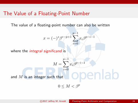
The Value of a Floating-Point Number
The value of a floating-point number can also be written
x = (−)sβe−p+1p−1∑i=0
xiβp−i−1
where the integral significand is
M =
p−1∑i=0
xiβp−i−1
and M is an integer such that
0 ≤M < βp
c©2017 Jeffrey M. Arnold Floating-Point Arithmetic and Computation 24
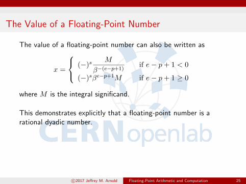
The Value of a Floating-Point Number
The value of a floating-point number can also be written as
x =
(−)sM
β−(e−p+1)if e− p+ 1 < 0
(−)sβe−p+1M if e− p+ 1 ≥ 0
where M is the integral significand.
This demonstrates explicitly that a floating-point number is arational dyadic number.
c©2017 Jeffrey M. Arnold Floating-Point Arithmetic and Computation 25

Requiring Uniqueness
x = (−)sβep−1∑i=0
xiβ−i
To make the combination of e and {xi} unique, x0 must benon-zero if possible.Otherwise, using binary radix (β = 2), 0.5 could be written as
• 2−1 × 1 · 20 (e = −1, x0 = 1)
• 20 × 1 · 2−1 (e = 0, x0 = 0, x1 = 1)
• 21 × 1 · 2−2 (e = 1, x0 = x1 = 0, x2 = 1)
• . . .
c©2017 Jeffrey M. Arnold Floating-Point Arithmetic and Computation 26

Requiring Uniqueness
This requirement to make x0 6= 0 if possible has the effect ofminimizing the exponent in the representation of the number.
However, the exponent is constrained to be in the rangeemin ≤ e ≤ emax.
Thus, if minimizing the exponent would result in e < emin, then x0
must be 0.
A non-zero floating-point number with x0 = 0 is called asubnormal number. The term “denormal”is also used.
c©2017 Jeffrey M. Arnold Floating-Point Arithmetic and Computation 27

Subnormal Floating-Point Numbers
m =
p−1∑i=0
xiβ−i
• If m = 0, then x0 = x1 = · · · = xp−1 = 0 and the value of thenumber is ±0
• If m 6= 0 and x0 6= 0, the number is a normal number with1 ≤ m < β
• If m 6= 0 but x0 = 0, the number is subnormal with0 < m < 1• The exponent of the value is emin
c©2017 Jeffrey M. Arnold Floating-Point Arithmetic and Computation 28

Why have Subnormal Floating-Point Numbers?
• Subnormals allow for “gradual”rather than “abrupt”underflow
• With subnormals, a = b⇔ a− b = 0
However, processing of subnormals can be difficult to implement inhardware
• Software intervention may be required
• May impact performance
c©2017 Jeffrey M. Arnold Floating-Point Arithmetic and Computation 29

Why p− 1?
• For normal numbers, x0 is always 1
• For subnormal numbers and zero, x0 is always 0
• There are many more normal numbers than subnormalnumbers
An efficient storage format:
• Don’t store x0 in memory; assume it is 1
• Use a special exponent value to signal a subnormal or zero;e = emin − 1 seems useful• thus E = 0 for both a value of 0 and for subnormals
c©2017 Jeffrey M. Arnold Floating-Point Arithmetic and Computation 30

A Walk Through the Doubles
0x0000000000000000 plus 00x0000000000000001 smallest subnormal...0x000fffffffffffff largest subnormal0x0010000000000000 smallest normal...0x001fffffffffffff
0x0020000000000000 2× smallest normal...0x7fefffffffffffff largest normal0x7ff0000000000000 +∞
c©2017 Jeffrey M. Arnold Floating-Point Arithmetic and Computation 31

A Walk Through the Doubles
0x7fefffffffffffff largest normal0x7ff0000000000000 +∞0x7ff0000000000001 NaN...0x7fffffffffffffff NaN0x8000000000000000 −0
c©2017 Jeffrey M. Arnold Floating-Point Arithmetic and Computation 32

A Walk Through the Doubles
0x8000000000000000 minus 00x8000000000000001 smallest -subnormal...0x800fffffffffffff largest -subnormal0x8010000000000000 smallest -normal...0x801fffffffffffff
...0xffefffffffffffff largest -normal0xfff0000000000000 −∞
c©2017 Jeffrey M. Arnold Floating-Point Arithmetic and Computation 33

A Walk Through the Doubles
0xffefffffffffffff largest -normal0xfff0000000000000 −∞0xfff0000000000001 NaN...0xffffffffffffffff NaN0x0000000000000000 Back to the beginning!
c©2017 Jeffrey M. Arnold Floating-Point Arithmetic and Computation 34

c©2017 Jeffrey M. Arnold Floating-Point Arithmetic and Computation 35

Notation
• Floating-point operations are written• ⊕ for addition• for subtraction• ⊗ for multiplication• � for division
• a⊕ b represents the floating-point addition of a and b• a and b are floating-point numbers• the result is a floating-point number• in general, a⊕ b 6= a+ b• similarly for , ⊗ and �
• fl(x) denotes the result of a floating-point operation usingthe current rounding mode• E.g., fl(a+ b) = a⊕ b
c©2017 Jeffrey M. Arnold Floating-Point Arithmetic and Computation 36

Some Inconvenient Properties of Floating-Point Numbers
Let a, b and c be floating-point numbers. Then
• a+ b may not be a floating-point number• a+ b may not always equal a⊕ b• Similarly for the operations −, × and /• Recall that floating-point numbers do not form a field
• (a⊕ b)⊕ c may not be equal to a⊕ (b⊕ c)• Similarly for the operations , ⊗ and �
• a⊗ (b⊕ c) may not be equal to (a⊗ b)⊕ (a⊕ c)• (1� a)⊗ a may not be equal to a
c©2017 Jeffrey M. Arnold Floating-Point Arithmetic and Computation 37

The Fused Multiply-Add Instruction (FMA)
• Computes (a× b) + c in a single instruction
• There is only one rounding• There are two roundings with sequential multiply and add
instructions
• May allow for faster and more accurate calculation of• matrix multiplication• dot product• polynomial evaluation
• Standardized in IEEE 754-2008
• Execution time similar to an add or multiply but latency isgreater.
c©2017 Jeffrey M. Arnold Floating-Point Arithmetic and Computation 38

The Fused Multiply-Add Instruction (FMA)
However... Use of FMA may change floating-point results
• fl(a× b+ c) is not always the same as (a⊗ b)⊕ c• The compiler may be allowed to evaluate an expression as
though it were a single operation
• Consider
double a, b, c;
c = a >= b ? std::sqrt(a * a - b * b) : 0;
There are values of a and b for which the computed value ofa * a - b * b is negative even though a>=b
c©2017 Jeffrey M. Arnold Floating-Point Arithmetic and Computation 39

The Fused Multiply-Add Instruction (FMA)
Consider the following example:
double x = 0x1 .3333333333333p+0;
double x1 = x*x;
double x2 = fma(x,x,0);
double x3 - fma(x, x, -x*x));
x = 0x1 .3333333333333p+0;
x1 = x*x = 0x1.70 a3d70a3d70ap +0
x2 = fma(x,x,0) = 0x1.70 a3d70a3d70ap +0
x3 = fma(x,x,-x*x) = -0x1.eb851eb851eb8p -55
x3 is the difference between the exact value of x*x and its valueconverted to double precision. The relative error is ≈ 0.24 ulp
c©2017 Jeffrey M. Arnold Floating-Point Arithmetic and Computation 40

The Fused Multiply-Add Instruction (FMA)
Floating-point contractions
• Evaluate an expression as though it were a single operation
double a, b, c, d;
// Single expression; maybe replaced
// by a = FMA(b, c, d)
a = b * c + d;
• Combine multiple expression into a single operation
double a, b, c, d;
// Multiple expressions; maybe replaced
// by a = FMA(b, c, d)
a = b; a *=c; a +=d;
c©2017 Jeffrey M. Arnold Floating-Point Arithmetic and Computation 41

The Fused Multiply-Add Instruction (FMA)
Contractions are controlled by compiler switch(es) and #pragmas
• -fpp-contract=on|off|fast
• #pragma STDC FP CONTRACT ON|OFF
IMPORTANT: Understand how your particular compilerimplements these features
• gcc behavor has changed over time and may change in thefuture
• clang behaves differently than gcc
c©2017 Jeffrey M. Arnold Floating-Point Arithmetic and Computation 42

Forward and Backward Errors
The problem we wish to solve is
f(x)→ y
but the problem we are actually solving is
f(x)→ y
Our hope is thatx = x+ ∆x ≈ x
andf(x) = f(x+ ∆x) = y ≈ y = f(x)
c©2017 Jeffrey M. Arnold Floating-Point Arithmetic and Computation 43

Forward and Backward Errors
For example, iff(x) = sin(x) and x = π
theny = 0
However, ifx = M PI
thenx 6= x and f(x) 6= f(x)
Note we are assuming that if x ≡ x then std::sin(x) ≡ sin(x)
c©2017 Jeffrey M. Arnold Floating-Point Arithmetic and Computation 44

Forward and Backward Errors
Absolute forward error: |y − y| = |∆y|
Relative forward error:|y − y||y|
=|∆y||y|
This requires knowing the exact value of y and that y 6= 0
Absolute backward error: |x− x| = |∆x|
Relative backward error:|x− x||x|
=|∆x||x|
This requires knowing the exact value of x and that x 6= 0
c©2017 Jeffrey M. Arnold Floating-Point Arithmetic and Computation 45

Forward and Backward Errors
By J.G. Nagy, Emory University. From Brief Notes on Conditioning, Stability and Finite Precision Arithmetic
c©2017 Jeffrey M. Arnold Floating-Point Arithmetic and Computation 46

Condition Number
• Well conditioned: small ∆x produces small ∆y
• Ill conditioned: small ∆x produces large ∆y
condition number =relative change in y
relative change in x
=
∣∣∣∆yy ∣∣∣∣∣∆xx
∣∣≈∣∣∣∣xf ′(x)
f(x)
∣∣∣∣
c©2017 Jeffrey M. Arnold Floating-Point Arithmetic and Computation 47

Condition Number
• ln x for x ≈ 1
Condition number ≈∣∣∣∣xf ′(x)
f(x)
∣∣∣∣ =
∣∣∣∣ 1
ln x
∣∣∣∣→∞• sin x for x ≈ π
Condition number ≈∣∣∣ x
sin x
∣∣∣→∞
c©2017 Jeffrey M. Arnold Floating-Point Arithmetic and Computation 48

Error Measures
ulp: ulp(x) is the place value of the least bit of the significand of xIf x 6= 0 and |x| = βe
∑p−1i=0 xiβ
−i, then ulp(x) = βe−p+1
c©2017 Jeffrey M. Arnold Floating-Point Arithmetic and Computation 49
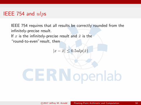
IEEE 754 and ulps
IEEE 754 requires that all results be correctly rounded from theinfinitely-precise result.If x is the infinitely-precise result and x is the“round-to-even”result, then
|x− x| ≤ 0.5ulp(x)
c©2017 Jeffrey M. Arnold Floating-Point Arithmetic and Computation 50

Approximation Error
const double a = 0.1;
const double b = 0.01;
• Both 0.1 and 0.01 are rational numbers but neither is afloating-point number
• The value of a is greater than 0.1 by ∼ 5.6× 10⁻¹⁸ or ∼ 0.4ulps
• The value of b is greater than 0.01 by ∼ 2.1× 10⁻¹⁹ or ∼ 0.1ulps
c©2017 Jeffrey M. Arnold Floating-Point Arithmetic and Computation 51

Approximation Error
const double a = 0.1;
const double b = 0.01;
double c = a * a;
• c is greater than b by 1 ulp or ∼ 1.7× 10⁻¹⁸
• c is greater than 0.01 by ∼ 1.9× 10⁻¹⁸ > 1 ulp
c©2017 Jeffrey M. Arnold Floating-Point Arithmetic and Computation 52
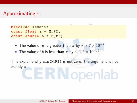
Approximating π
#include <cmath >
const float a = M_PI;
const double b = M_PI;
• The value of a is greater than π by ∼ 8.7× 10⁻⁸
• The value of b is less than π by ∼ 1.2× 10⁻¹⁶
This explains why sin(M PI) is not zero: the argument is notexactly π
c©2017 Jeffrey M. Arnold Floating-Point Arithmetic and Computation 53
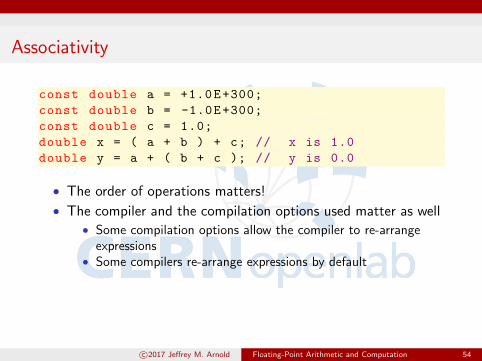
Associativity
const double a = +1.0E+300;
const double b = -1.0E+300;
const double c = 1.0;
double x = ( a + b ) + c; // x is 1.0
double y = a + ( b + c ); // y is 0.0
• The order of operations matters!
• The compiler and the compilation options used matter as well• Some compilation options allow the compiler to re-arrange
expressions• Some compilers re-arrange expressions by default
c©2017 Jeffrey M. Arnold Floating-Point Arithmetic and Computation 54

Distributivity
const double a = 10.0/3.0;
const double b = 0.1;
const double c = 0.2;
double x = a * (b + c);
// x is 0x1 .0000000000001p+0
double y = (a * b) + (a * c);
// y is 0x1 .0000000000000p+0
• Again, the order of operations, the compiler and thecompilation options used all matter
c©2017 Jeffrey M. Arnold Floating-Point Arithmetic and Computation 55

The “Pigeonhole”Principle
• You have n+ 1 pigeons (i.e., discrete objects)
• You put them into n pigeonholes (i.e., boxes)
• At least one pigeonhole contains more than one pigeon.
c©2017 Jeffrey M. Arnold Floating-Point Arithmetic and Computation 56

The “Pigeonhole”Principle
An example of using the ”Pigeonhole” Principle:
• The number of IEEE Binary64 numbers in [1, 2) is N = 252
• The number of IEEE Binary64 numbers in [1, 4) is 2N
• Each value in [1, 4) has its square root in (1, 2]
• Since there are more values in [1, 4) than in [1, 2), there mustbe at least two distinct floating-point numbers in [1, 4) whichhave the same square root
c©2017 Jeffrey M. Arnold Floating-Point Arithmetic and Computation 57
Catastrophic Cancellation
Catastrophic cancellation occurs when two nearly equalfloating-point numbers are subtracted.
If x ≈ y, their signifcands are nearly identical. When they aresubtracted, only a few low-order digits remain. I.e., the result hasvery few significant digits left.
c©2017 Jeffrey M. Arnold Floating-Point Arithmetic and Computation 58

Sterbenz’s Lemma
Lemma
Let a and b be floating-point numbers with
b/2 ≤ a ≤ 2b
. If subnormal numbers are available, a b = a− b.
Thus there is no rounding error associated with a b when a and bsatisfy the criteria.
However, there may be lost of significance.
c©2017 Jeffrey M. Arnold Floating-Point Arithmetic and Computation 59

Error-Free Transformations
An error-free transformation (EFT) is an algorithm whichtransforms a (small) set of floating-point numbers into another(small) set of floating-point numbers of the same precision withoutany loss of information.
f(x, y) 7−→ (s, t)
c©2017 Jeffrey M. Arnold Floating-Point Arithmetic and Computation 60

Error-Free Transformations
EFTs are most useful when they can be implemented using onlythe precision of the floating-point numbers involved.
EFTs exist for
• Addition: a+ b = s+ t where s = a⊕ b• Multiplication: a× b = s+ t where s = a⊗ b• Splitting: a = s+ t
Additional EFTs can be derived by composition. For example, anEFT for dot products makes use of those for addition andmultiplication.
c©2017 Jeffrey M. Arnold Floating-Point Arithmetic and Computation 61

An EFT for Addition
Require: |a| ≥ |b|1: s← a⊕ b2: t← b (s a)3: return (s, t)
Ensure: a+ b = s+ t where s = a⊕ b and t are floating-pointnumbers
A possible implementation
void
FastSum(const double a, const double b,
double * const s, double * const t) {
// No unsafe optimizations!
*s = a+b;
*t = b-(*s-a);
return;
}c©2017 Jeffrey M. Arnold Floating-Point Arithmetic and Computation 62

Another EFT for Addition: TwoSum
1: s← a⊕ b2: z ← s a3: t← (a (s z)⊕ (b z)4: return (s, t)
Ensure: a+ b = s+ t where s = a⊕ b and t are floating-pointnumbers
A possible implementation
void
TwoSum(const double a, const double b,
double * const s, double * const t) {
// No unsafe optimizations!
*s = a+b;
double z = *s-a;
*t = (a-(*s-z))+(b-a);
return;
} c©2017 Jeffrey M. Arnold Floating-Point Arithmetic and Computation 63
Comparing FastSum and TwoSum
• A realistic implementation of FastSum requires a branch and3 floating-point opertions
• TwoSum takes 6 floating-point operations but requires nobranches
• TwoSum is usually faster on modern pipelined processors
• The algorithm used in TwoSum is valid in radix 2 even ifunderflow occurs but fails with overflow
c©2017 Jeffrey M. Arnold Floating-Point Arithmetic and Computation 64

Precise Splitting Algorithm
• Given a base-2 floating-point number x, determine thefloating-point numbers xh and xl such that x = xh + xl
• For 0 < δ < p, where p is the precision and δ is a parameter,• The signficand of xh fits in p− δ bits• The signficand of xl fits in δ − 1 bits• All other bits are 0• δ is typically chosed to be dp/2e
• No information is lost in the transformation• Aside: how do we end up only needing
(p− δ) + (δ − 1) = p− 1 bits?
• This scheme is known as Veltkamp’s algorithm
c©2017 Jeffrey M. Arnold Floating-Point Arithmetic and Computation 65

Precise Splitting EFT
Require: C = 2s + 1; C ⊗ x does not overflow1: a← C ⊗ x2: b← x a3: xh ← a⊕ b4: xl ← x xh5: return (xh, xl)
Ensure: x = xh + xl
c©2017 Jeffrey M. Arnold Floating-Point Arithmetic and Computation 66

Precise Splitting EFT
Possible implementation
void
Split(const double x, const int delta ,
double * const x_h , double * const x_l) {
// No unsafe optimizations!
double c = (double )((1UL << delta) + 1);
*x_h = (c * x) + (x - (c * x));
*x_l = x - *x_h;
return;
}
c©2017 Jeffrey M. Arnold Floating-Point Arithmetic and Computation 67

Precise Multiplication
• Given floating-point numbers x and y, determinefloating-point numbers s and t such that a× b = s+ t wheres = a⊗ b and
t = ((((xh ⊗ yh) s)⊕ (xh ⊗ yl))⊕ (xl ⊗ yh))⊕ (xl ⊗ yl).
• Known as Dekker’s algorithm
c©2017 Jeffrey M. Arnold Floating-Point Arithmetic and Computation 68

Precise Multiplication EFT
The algorithm is much simpler using FMA
1: s← x⊗ y2: t← FMA(x, y,−s)3: return (s, t)
Ensure: x ∗ y = s+ t where s = x⊗ y and t are floating-pointnumbers
Possible implementation
void
Prod(const double a, const double b,
double * const s, double * const t) {
// No unsafe optimizations!
*s = a * b;
*t = FMA(a, b, -*s);
return;
}c©2017 Jeffrey M. Arnold Floating-Point Arithmetic and Computation 69

Summation Techniques
• Traditional
• Sorting and Insertion
• Compensated
• Reference: Higham: Accuracy and Stability of NumericalAlgorithms
c©2017 Jeffrey M. Arnold Floating-Point Arithmetic and Computation 70

Summation Techniques
Condition number:
Csum =
∑i |xi|
|∑
i xi|
• If Csum is not too large, the problem is not ill-conditioned andtraditional methods may be sufficient
• If Csum is too large, we need to have results appropriate to ahigher precision without actually using a higher precision
• Obviously, if higher precision is readily available, use it
c©2017 Jeffrey M. Arnold Floating-Point Arithmetic and Computation 71

Traditional Summation
s =
n−1∑i=0
xi
double
Sum(const double* x, const unsigned int n)
{ // No unsafe optimizations!
double sum = x[0]
for(unsigned int i = 1; i < n; i++) {
sum += x[i];
}
return;
}
c©2017 Jeffrey M. Arnold Floating-Point Arithmetic and Computation 72

Sorting and Insertion
• Reorder the operands• By value or magnitude• Increasing or decreasing
• Insertion• First sort by magnitude• Remove x1 and x2 and compute their sum• Insert that value into the list keeping the list sorted• Repeat until only one element is in the list
• Many Variations• If lots of cancellations, sorting by decreasing magnitude may
be better but not always
c©2017 Jeffrey M. Arnold Floating-Point Arithmetic and Computation 73

Compensated Summation
• Based on FastTwoSum and TwoSum techniques
• Knowledge of the exact rounding error in a floating-pointaddition is used to correct the summation
• Developed by William Kahan
c©2017 Jeffrey M. Arnold Floating-Point Arithmetic and Computation 74

Compensated (Kahan) Summation
Function Kahan (x,n)Input: n > 0s← x0
t← 0for i = 1 to n− 1 do
y ← xi − t // Apply correction
z ← s+ y // New sum
t← (z − s)− y // New correction ≈ low part of y
s← z // Update sum
endreturn s
c©2017 Jeffrey M. Arnold Floating-Point Arithmetic and Computation 75

Compensated (Kahan) Summation
double
Kahan(const double* x, const unsigned int n)
{ // No unsafe optimizations!
double s = x[0];
double t = 0.0;
for( int i = 1; i < n_values; i++ ) {
double y = x[i] - t;
double z = s + y;
t = ( z - s ) - y;
s = z;
}
return s;
}
c©2017 Jeffrey M. Arnold Floating-Point Arithmetic and Computation 76

Compensated Summation
Many variations known. Consult the literature for papers withthese authors:
• William M Kahan
• Donald Knuth
• Douglas Priest
• S M Rump, T Ogita and S Oishi
• Jonathan Shewchuk
• AriC project (CNRS/ENS Lyon/INRIA)
c©2017 Jeffrey M. Arnold Floating-Point Arithmetic and Computation 77

Choice of Summation Technique
• Performance
• Error Bound• Is it (weakly) dependent on n?
• Condition Number• Is it known?• Is it difficult to determine?• Some algorithms allow it to be determined simultaneously with
an estimate of the sum• Permits easy evaluation of the suitability of the result
• No one technique fits all situations all the time
c©2017 Jeffrey M. Arnold Floating-Point Arithmetic and Computation 78

Dot Product
S = xᵀy
=
n−1∑i=0
xi · yi
where x and y are vectors of length n.
c©2017 Jeffrey M. Arnold Floating-Point Arithmetic and Computation 79

Dot Product
Traditional algorithm
Require: x and y are n-dimensional vectors with n ≥ 01: s← 02: for i = 0 to n− 1 do3: s← s⊕ (xi ⊗ yi)4: end for5: return s
c©2017 Jeffrey M. Arnold Floating-Point Arithmetic and Computation 80
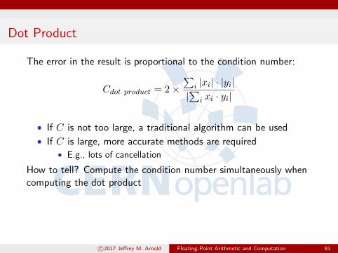
Dot Product
The error in the result is proportional to the condition number:
Cdot product = 2×∑
i |xi| · |yi||∑
i xi · yi|
• If C is not too large, a traditional algorithm can be used
• If C is large, more accurate methods are required• E.g., lots of cancellation
How to tell? Compute the condition number simultaneously whencomputing the dot product
c©2017 Jeffrey M. Arnold Floating-Point Arithmetic and Computation 81
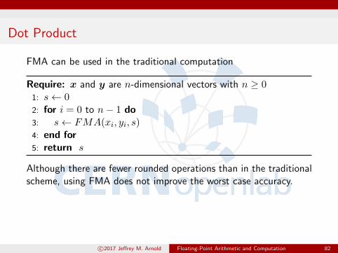
Dot Product
FMA can be used in the traditional computation
Require: x and y are n-dimensional vectors with n ≥ 01: s← 02: for i = 0 to n− 1 do3: s← FMA(xi, yi, s)4: end for5: return s
Although there are fewer rounded operations than in the traditionalscheme, using FMA does not improve the worst case accuracy.
c©2017 Jeffrey M. Arnold Floating-Point Arithmetic and Computation 82

Dot Product
Recall
• Sum(x, y) computes s and t with x+ y = s+ t and s = x⊕ y• Prod(x, y) computes s and t with x+ y = s+ t and s = x⊗ y
Since each individual product in the sum for the dot product istransformed using Prod(x, y) into the sum of two floating-pointnumbers, the dot product of 2 vectors can be reduced tocomputing the sum of 2N floating-point numbers.
To accurately compute that sum, Sum(x, y) is used.
c©2017 Jeffrey M. Arnold Floating-Point Arithmetic and Computation 83

Dot Product
Compensated dot product algorithm
Require: x and y are n-dimensional vectors with n ≥ 01: (sh, sl)← (0, 0)2: for i = 0 to n− 1 do3: (ph, pl)← Prod(xi, yi)4: (sh, a)← Sum(sh, ph)5: sl ← sl ⊕ (pl ⊕ a)6: end for7: return sh ⊕ sl
The relative accuracy of this algorithm is the same as thetraditional algorithm when computed using twice the precision.
c©2017 Jeffrey M. Arnold Floating-Point Arithmetic and Computation 84

Polynomial Evaluation
Evaluate
p(x) =
n∑i=0
aixi
= a0 + a1x+ a2x2 + · · ·+ an−1x
n−1 + anxn
Condition number
C(p, x) =
∑ni=0 |ai| |x|
i
|∑n
i=0 aixi|
Note that C(p, x) = 1 for certain combinations of a and x. E.g., ifai ≥ 0 for all i and x ≥ 0.
c©2017 Jeffrey M. Arnold Floating-Point Arithmetic and Computation 85

Horner’s Scheme
Nested multiplication is a standard method for evaluating p(x):
p(x) = (((anx+ an−1)x+ an−2)x · · ·+ a1)x+ a0
This is known as Horner’s scheme (although Newton published itin 1711!)
c©2017 Jeffrey M. Arnold Floating-Point Arithmetic and Computation 86
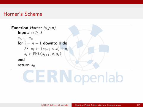
Horner’s Scheme
Function Horner (x,p,n)Input: n ≥ 0sn ← anfor i = n− 1 downto 0 do
// si ← (si+1 × x) + aisi ←FMA(si+1, x, ai)
endreturn s0
c©2017 Jeffrey M. Arnold Floating-Point Arithmetic and Computation 87

Horner’s Scheme
A possible implementation
double
Horner(const double x,
const double * const a,
const int n) {
double s = a[ n ];
for (int i = n - 1; i >= 0; i--} (
// s = s * x + a[ i ];
s = FMA(s, x, a[ i ]);
}
return s;
}
c©2017 Jeffrey M. Arnold Floating-Point Arithmetic and Computation 88

Applying EFTs to Horner’s Scheme
Horner’s scheme can be improved by applying the EFTs Sum andProd
Function HornerEFT (x,p,n)Input: n ≥ 0sn ← anfor i = n− 1 downto 0 do
(pi, πi)← Prod(si+1, x)(si, σi)← Sum(pi, ai)
endreturn s0, π, σ
The value of s0 calculated by this algorithm is the same as thatusing the traditional Horner’s scheme.
c©2017 Jeffrey M. Arnold Floating-Point Arithmetic and Computation 89
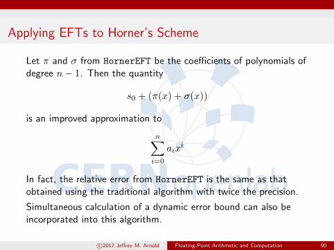
Applying EFTs to Horner’s Scheme
Let π and σ from HornerEFT be the coefficients of polynomials ofdegree n− 1. Then the quantity
s0 + (π(x) + σ(x))
is an improved approximation to
n∑i=0
aixi
In fact, the relative error from HornerEFT is the same as thatobtained using the traditional algorithm with twice the precision.
Simultaneous calculation of a dynamic error bound can also beincorporated into this algorithm.
c©2017 Jeffrey M. Arnold Floating-Point Arithmetic and Computation 90

Second Order Horner’s Scheme
Horner’s scheme is sequential: each step of the calculation dependson the result of the preceeding step.
Consider
p(x) = a0 + a1x+ a2x2 + · · ·+ an−1x
n−1 + anxn
= (a0 + a2x2 + · · · ) + x(a1 + a3x
2 + · · · )= q(x2) + xr(x2)
• The calculations of q(x2) and r(x2) can be done in parallel
• This technique may be applied recursively
c©2017 Jeffrey M. Arnold Floating-Point Arithmetic and Computation 91

Estrin’s Method
Isolate subexpressions of the form (ak + ak+1x) and x2n from p(x):
p(x) = (ao+a1x)+(a2+a3x)x2+((a4+a5x)+(a6+a7x)x2)x4+· · ·
The subexpressions (ak + ak+1x) can be evaluated in parallel
c©2017 Jeffrey M. Arnold Floating-Point Arithmetic and Computation 92

Value Safety
“Value Safety”refers to transformations which, althoughalgebraically valid, may affect floating-point results.
Ensuring “Value Safety”requires that no optimizations be donewhich could change the result of any series of floating-pointoperations as specified by the programming language.
• Changes to underflow or overflow behavior
• Effects of an operand which is not a finite floating-pointnumber. E.g., ±∞ or a NaN
Transformations which violate “Value Safety”are not error freetransformations.
c©2017 Jeffrey M. Arnold Floating-Point Arithmetic and Computation 93

Value Safety
In “safe”mode, the compiler may not make changes such as
(x+ y) + z ⇔ x+ (y + z) Reassociations are not value-safex ∗ (y + z)⇔ x ∗ y + x ∗ z Distributions are not value-safex ∗ (y ∗ z)⇔ (x ∗ y) ∗ z May change under-/overflow behaviorx/x⇔ 1.0 x may be 0, ∞ or a NaNx+ 0⇔ x x may be −0 or a NaNx ∗ 0⇔ 0 x may be −0, ∞ or a NaN
c©2017 Jeffrey M. Arnold Floating-Point Arithmetic and Computation 94

A Note on Compiler Options
• There are many compiler options which affect floating-pointresults
• Not all of them are obvious
• Some of them are enabled/disabled by other options• -On• -march and others which specify platform characteristics
• Options differ among compilers
c©2017 Jeffrey M. Arnold Floating-Point Arithmetic and Computation 95
Optimizations Affecting Value Safety
• Expression rearrangements
• Flush-to-zero
• Approximate division and square root
• Math library accuracy
c©2017 Jeffrey M. Arnold Floating-Point Arithmetic and Computation 96

Expression Rearrangements
These rearrangements are not value-safe:
• (a⊕ b)⊕ c⇒ a⊕ (b⊕ c)• a⊗ (b⊕ c)⇒ (a⊗ b)⊕ (a⊕ c)
To disallow these changes:
gcc Don’t use -ffast-math
icc Use -fp-model precise
• Recall that options such as -On are “aggregated”or“composite”options• they enable/disable many other options• their composition may change with new compiler releases
Disallowing rearrangements may affect performance
c©2017 Jeffrey M. Arnold Floating-Point Arithmetic and Computation 97

Subnormal Numbers and Flush-To-Zero
• Subnormal numbers extend the range of floating-pointnumbers but with reduced precision and reduced performance
• If you do not require subnormals, disable their generation
• “Flush-To-Zero”means “Replace all generated subnormalswith 0”• Note that this may affect tests for == 0.0 and != 0.0
• If using SSE or AVX, this replacement is fast since it is doneby the hardware
c©2017 Jeffrey M. Arnold Floating-Point Arithmetic and Computation 98

Subnormal Numbers and Flush-To-Zero
gcc -ffast-math enables flush-to-zero
gcc But -O3 -ffast-math disables flush-to-zero
icc Done by default at -O1 or higher
icc Use of -no-ftz or fp-model precise to will prevent this
icc Use -fp-model precise -ftz to get both “precise”behaviorand subnormals
• Options must be applied to the program unit containing main
as well
c©2017 Jeffrey M. Arnold Floating-Point Arithmetic and Computation 99

Reductions
• Summation is an example of a reduction
• Parallel implementations of reductions are inherentlyvalue-unsafe because they may change the order of operations• the parallel implementation can be through vectorization or
multi-threading or both• there are OpenMP and TBB options to make reductions
“reproducible”• For OpenMP KMP DETERMINSTIC REDUCTION=yes
icc use of -fp-model precise disables automatic vectorizationand automatic parallelization via threading
c©2017 Jeffrey M. Arnold Floating-Point Arithmetic and Computation 100

The Hardware Floating-Point Environment
The hardware floating-point environment is controled by severalCPU control words
• Rounding mode
• Status flags
• Exception mask
• Control of subnormals
If you change anything affecting the assumed state of the processorwith respect to floating-point behavior, you must tell the compiler
• Use #pragma STDC FENV ACCESS ON
icc Use -fp-model strict
#pragma STDC FENV ACCESS ON is required if flags are accessed
c©2017 Jeffrey M. Arnold Floating-Point Arithmetic and Computation 101

Precise Exceptions
Precise Exceptions: floating-point exceptions are reported exactlywhen they occur
To enable precision exceptions
• Use #pragma float control(except, on)
icc Use -fp-model strict or -fp-model except
Enabling precise exceptions disables speculative execution offloating-point instructions. This will probably affect performance.
c©2017 Jeffrey M. Arnold Floating-Point Arithmetic and Computation 102

Math Library Features – icc
A variety of options to control precision and consistency of results
• -fimf-precision=<high|medium|low>[:funclist]
• -fimf-arch-consistency=<true|false>[:funclist]
• And several more options• -fimf-absolute-error=<value>[:funclist]• -fimf-accuracy-bits=<value>[:funclist]• . . .
c©2017 Jeffrey M. Arnold Floating-Point Arithmetic and Computation 103

Tools
• double-double and quad-double data types• Implemented in C++• Fortran 90 interfaces provided• Available from LBL as qd-X.Y.Z.tar.gz• ”LBNL-BSD” type license
c©2017 Jeffrey M. Arnold Floating-Point Arithmetic and Computation 104

Tools
GMP – The GNU Multiple Precision Arithmetic Library
• a C library
• arbitrary precision arithmetic for• signed integers• rational numbers• floating-point numbers
• used by gcc and g++ compilers
• C++ interfaces
• GNU LGPL license
c©2017 Jeffrey M. Arnold Floating-Point Arithmetic and Computation 105

Tools
MPFR
• a C library for multiple-precision floating-point computations
• all results are correctly rounded
• used by gcc and g++
• C++ interface available
• free with a GNU LGPL license
c©2017 Jeffrey M. Arnold Floating-Point Arithmetic and Computation 106

Tools
CRlibm
• a C library
• all results are correctly rounded
• C++ interface available
• Python bindings available
• free with a GNU LGPL license
c©2017 Jeffrey M. Arnold Floating-Point Arithmetic and Computation 107

Tools
• limits
• defines characteristics of arithmetic types• provides the template for the class numeric limits• #include <limits>• requires -std=c++11• specializations for each fundamental type• compiler and platform specific
c©2017 Jeffrey M. Arnold Floating-Point Arithmetic and Computation 108

Tools
• cmath
• functions to compute common mathematical operations andtransformations
• #include <cmath>• frexp
• get exponent and significand
• ldexp
• create value from exponent and significand
• Note: frexp and ldexp assume a different“normalization”than usual: 1/2 ≤ m < 1
• nextafter
• create next representable value
• fpclassify
• returns one of FP INFINITE, FP NAN, FP ZERO,
F SUBNORMAL, FP NORMAL
c©2017 Jeffrey M. Arnold Floating-Point Arithmetic and Computation 109

Pitfalls and Gremlins
Catastrophic Cancellation
• x2 − y2 for x ≈ y• (x+ y)(x− y) may be preferable• x− y is computed with no round-off error (Sterbenz’s Lemma)• x+ y is computed with relatively small error
• FMA(x,x,-y*y) can be very accurate• However FMA(x,x,-x*x) is not usually 0!
• similarly 1− x2 for x ≈ 1• -FMA(x,x,-1.0) is very accurate
c©2017 Jeffrey M. Arnold Floating-Point Arithmetic and Computation 110

Pitfalls and Gremlins
“Gratuitous”Overflow
Consider√x2 + 1 for large x
•√x2 + 1→ |x| as |x| → ∞
• |x|√
1 + 1/x2 may be preferable• if x2 overflows, 1/x→ 0• |x|
√1 + 1/x2 → |x|
c©2017 Jeffrey M. Arnold Floating-Point Arithmetic and Computation 111

Pitfalls and Gremlins
Consider the Newton-Raphson iteration for 1/√x:
yn+1 ← yn(3− xy2n)/2
where yn ≈ 1/√x. Since xy2
n ≈ 1, there is at most an alignmentshift of 2 when computing 3− xy2
n, and the final operation consistsof multiplying yn by a computed quantity near 1. (The division by2 is exact.)
If the iteration is rewritten as
yn + yn(1− xy2n)/2,
the final addition involves a large alignment shift between yn andthe correction term yn(1− xy2
n)/2 avoiding cancellation.
c©2017 Jeffrey M. Arnold Floating-Point Arithmetic and Computation 112

Pitfalls and Gremlins
This situation can be generalized:
When calculating a quantity from other calculated (i.e., inexact)values, try to formulate the expressions so that the final operationis an addition of a smaller “correction”term to a value which isclose to the final result.
c©2017 Jeffrey M. Arnold Floating-Point Arithmetic and Computation 113
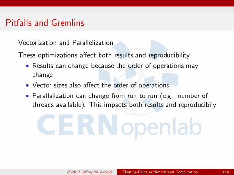
Pitfalls and Gremlins
Vectorization and Parallelization
These optimizations affect both results and reproducibility
• Results can change because the order of operations maychange
• Vector sizes also affect the order of operations
• Parallalization can change from run to run (e.g., number ofthreads available). This impacts both results and reproducibily
c©2017 Jeffrey M. Arnold Floating-Point Arithmetic and Computation 114
Pitfalls and Gremlins
And finally... CPU manufacturer can impact results. Not allfloating-point instructions execute exactly the same on AMD andIntel processors
• The rsqrt and rcp instructions differ
• They are not standardized
• Both implementations meet the specification given by Intel
The exact same non-vectorized, non-parallelized, non-threadedapplication may give different results on systems with similarprocessors each vendor.
c©2017 Jeffrey M. Arnold Floating-Point Arithmetic and Computation 115

Pitfalls and Gremlins
And undoubtedly others, as yet undiscovered.
c©2017 Jeffrey M. Arnold Floating-Point Arithmetic and Computation 116

Bibliography
J.-M. Muller et al, Handbookof Floating-Point Arithmetic,Birkauser, Boston, 2010
c©2017 Jeffrey M. Arnold Floating-Point Arithmetic and Computation 117

Bibliography
J.-M. Muller, Elementary Functions,Algorithms and Implementation (2nd
Edition), Birkauser, Boston, 2006
c©2017 Jeffrey M. Arnold Floating-Point Arithmetic and Computation 118

Bibliography
N.J. Higham, Accuracy and Stabilityof Numerical Algorithms (2nd
Edition), Siam, Philadelphia, 2002.
c©2017 Jeffrey M. Arnold Floating-Point Arithmetic and Computation 119

Bibliography
• IEEE, IEEE Standard for Floating-Point Arithmetic, IEEEComputer Society, August 2008.
• D. Goldberg, What every computer scientist should knowabout floating-point arithmetic, ACM Computing Surverys,23(1):5-47, March 1991
• Publications from CNRS/ENS Lyon/INRIA/AriC project(J.-M. Muller et al).
• Publications from the PEQUAN project at LIP6, UniversitePierre et Marie Curie (Stef Graillat, Christoph Lauter et al).
• Publications from Institut fur Zuverlassiges Rechnen (Institutefor Reliable Computing), Technische UniversitatHamburg-Harburg (Siegfried Rump et al).
c©2017 Jeffrey M. Arnold Floating-Point Arithmetic and Computation 120

c©2017 Jeffrey M. Arnold Floating-Point Arithmetic and Computation 121

c©2017 Jeffrey M. Arnold Floating-Point Arithmetic and Computation 122