an introduction to fortran 90 - uni-wuerzburg.de · 4 chapter 2 – an introduction to fortran 90...
TRANSCRIPT
2An Introduction to Fortran 90
This chapter aims at giving a short introduction to Fortran 90. As describing all featuresof the Fortran language would probably fill some hundred pages, we will concentrateon the basic features that will be needed to follow the rest of this textbook. Nevertheless,there are various Fortran tutorials out in the internet that could be used as complementaryliterature.
2.1 About Fortran in general
2.1.1 The history of Fortran
Fortran is pretty old. Actually it is considered the first realized higher programming lan-guage. It goes back to a proposal by John W. Backus, an IBM programmer, in 1953. Theterm Fortran is derived from The IBM Formula Translation System. Before the release of thefirst Fortran compiler in April 1957, people used to use assembly languages. The intro-duction of a higher programming language compiler reduced the number of code linesneeded to write a program tremendously and therefore FORTRAN, the first release ofthe Fortran programming language, grew pretty fast in popularity. From 1957 on severalversions followed the initial FORTRAN version, namely FORTRAN II and FORTRANIII in 1958 and FORTRAN IV in 1961. In 1966, the American Standards Association (nowknown as the ANSI) approved a standardized American Standard Fortran. The program-ming language defined on this standard was called FORTRAN 66. Approving an updatedstandard in 1977, the ANSI paved the way for a new Fortran version known as FORTRAN77. This version became pretty popular in computational economics during the 80ies andbeginning 90ies. More than 13 years later, the Fortran 90 standard was released by bothISO and ANSI in consecutive years. With FORTRAN 90, the fixed format standard wasexchanged by a free format standard. In addition, many new features like modules, recur-sive procedures, derived data types and dynamic memory allocation made the languagemuch more flexible. From Fortran 90 on, there has only been one major revision whichbasically introduced object-oriented programming features into the Fortran language in2003. However, as object-oriented programming will not be needed and Fortran 90 is byfar the more popular language, we will focus on the 1990 version in this book.
4 Chapter 2 – An Introduction to Fortran 90
2.1.2 Why to use Fortran
Fortran is a general purpose, procedural, imperative, high-level programming language.In detail this means that (a) Fortran was not created for a special purpose like e.g. Matlab,Mathematica or Gauss were for efficiently dealing with matrices or solving mathematicalproblems, (b) Fortran code that will be used several times can be stored in functions andsubroutines that can be called from other program parts, (c) a Fortran program consists ofstatements that will be executed one after the other (i.e. a Fortran program starts with thefirst line and ends with the last), and (d) Fortran abstracts from the details of a computer,i.e. having the right compiler, Fortran code could be run on every computer independentof its hardware configuration and operating system.
At this point our students usually ask "So, why to use Fortran? Why not a special pur-pose language or something more "fashionable" like Java?". Let us come up with somejustifying points. First, special purpose languages might be relatively efficient in the spe-cific purpose they were created for, however, slow in other areas. Matlab, for example,is very good in working with matrices of regular or sparse nature. However, if you haveever tried to run some do-loops in Matlab, you will know what we mean. Second, whenit comes to the more "fashionable" languages like Java or C++, one has to always keepin mind that those languages are usually object-oriented and abundant. They are verygood for creating software with Graphical User Interfaces, but not for running numericalmaths code quickly and efficiently. As computational economics usually consists of atleast 80% numerical methods, we need a programming language that is efficient in exe-cuting do-loops and if-statements, calling functions and subroutines and allows to per-manently store general code that is frequently used. Fortran is a language that matchesall those features and not much more. The only real alternative we know would be C.There is no real reason why not to use C instead of Fortran, it’s just a matter of preference.Last but not least, Fortran has been used a lot by engineers, numerical mathematiciansand computational economists during the 80ies and 90ies where a lot of optimizers andinterpolation techniques were written. Fortunately, Fortran 90 is backward compatiblewith FORTRAN 77, i.e. all the code that is out there can be easily included in our Fortranprograms.
All in all, it seems reasonable for us to have chosen a language that matches all the fea-tures we need but does not come with any unnecessary extras that just make executionless efficient.
2.1.3 The way high-level programming languages work
Low-level assembly languages that are basically used to program computers, micropro-cessors, etc. do not abstract from the computer’s instruction set architecture. Therefore,the syntax of assembly languages depends on the specific physical or virtual computerused. In addition, assembly languages are quite complicated and even a small programm
2.1. About Fortran in general 5
requires many lines of computer code.
In opposite to that, high-level programming languages abstract from the system architec-ture and are therefore portable between different systems. As in all other languages, onehas to learn the vocabulary, grammar, and punctuation called syntax of that language.However, compared to real languages, the syntax of a high-level language can be learnedwithin some hours. In addition, the semantics, i.e. the meaning or interpretation of thedifferent symbols you use, usually follows principles that can be comprehended by usingpure logic.
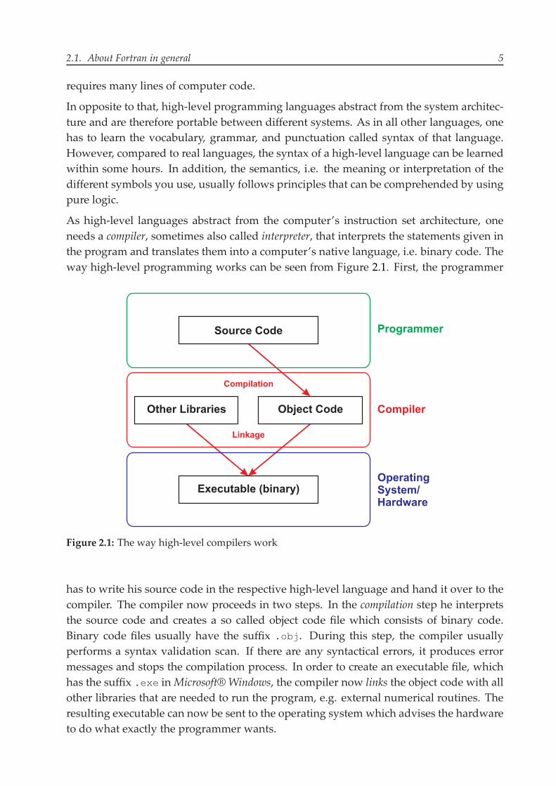
As high-level languages abstract from the computer’s instruction set architecture, oneneeds a compiler, sometimes also called interpreter, that interprets the statements given inthe program and translates them into a computer’s native language, i.e. binary code. Theway high-level programming works can be seen from Figure 2.1. First, the programmer
Programmer
Compiler
OperatingSystem/Hardware
Source Code
Executable (binary)
Compilation
Linkage
Other Libraries Object Code
Figure 2.1: The way high-level compilers work
has to write his source code in the respective high-level language and hand it over to thecompiler. The compiler now proceeds in two steps. In the compilation step he interpretsthe source code and creates a so called object code file which consists of binary code.Binary code files usually have the suffix .obj. During this step, the compiler usuallyperforms a syntax validation scan. If there are any syntactical errors, it produces errormessages and stops the compilation process. In order to create an executable file, whichhas the suffix .exe inMicrosoft® Windows, the compiler now links the object code with allother libraries that are needed to run the program, e.g. external numerical routines. Theresulting executable can now be sent to the operating system which advises the hardwareto do what exactly the programmer wants.
6 Chapter 2 – An Introduction to Fortran 90
2.1.4 Fortran Compilers for Windows® and Linux
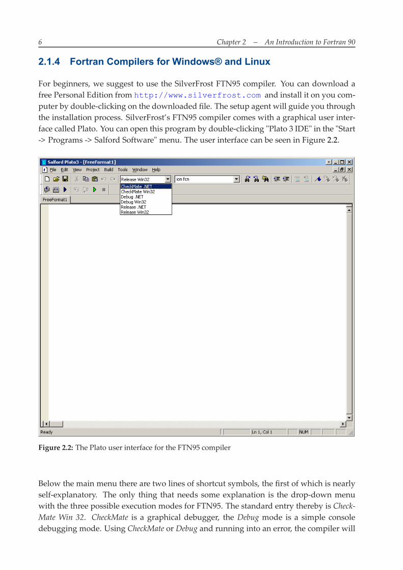
For beginners, we suggest to use the SilverFrost FTN95 compiler. You can download afree Personal Edition from http://www.silverfrost.com and install it on you com-puter by double-clicking on the downloaded file. The setup agent will guide you throughthe installation process. SilverFrost’s FTN95 compiler comes with a graphical user inter-face called Plato. You can open this program by double-clicking "Plato 3 IDE" in the "Start-> Programs -> Salford Software" menu. The user interface can be seen in Figure 2.2.
Figure 2.2: The Plato user interface for the FTN95 compiler
Below the main menu there are two lines of shortcut symbols, the first of which is nearlyself-explanatory. The only thing that needs some explanation is the drop-down menuwith the three possible execution modes for FTN95. The standard entry thereby is Check-Mate Win 32. CheckMate is a graphical debugger, the Debug mode is a simple consoledebugging mode. Using CheckMate or Debug and running into an error, the compiler will
2.1. About Fortran in general 7
give us detailed information about what happened and where exactly it occurred. In op-posite to that, Releaseminimizes the debug information in our programm which makes itrun pretty quick. Note, however, that the Release mode should only be used, if the pro-gram is fully developed and free of bugs. Please only use theWin32 modes, as the .NETmodes are only conceived for users that want to integrate the FTN95 compiler into aMi-crosoft® .NET Framework. Using the .NET mode without having the compiler properlyintegrated into the framework can produce weird results.1 The text field and the threebuttons on the right of the execution mode choice menu are used to search within a pro-gram or a file. The next two buttons increase and decrease the intent of code, respectively.The two buttons on the right of the intent buttons comment or uncomment some codelines. The last four buttons finally can be used to toggle bookmarks.
In order to demonstrate the usage of the second line of shortcut symbols, we first have towrite a small program. You can start a new program by creating a Free Format FortranSource File via using the "File -> New" button and typing some program code. Alterna-tively, you could open the file prog2_01.f90 from the program database that accompa-nies this book. The easiest example given in any computational textbook usually is theHello World program shown in Program 2.1.
Program 2.1: Hello World
program HelloWorld
write(*,*)’Hello World’
end program
A Fortran program always begins with the word program indicating that the programstarts here. After that, one has to declare the program’s name, which must follow theFortran naming conventions, i.e.
1. the name can’t have more than 31 characters,
2. it must start with a letter,
3. the other characters may be of any kind including symbols,
4. capital letters may be used but the compiler is case insensitive, and
5. the name must not be a valid Fortran command.
Finally, the program ends with end program. In between these two statements, we canwrite the general program code which will be executed in an imperative way, i.e. theprogram starts with the first line and ends with the last. In the case of Program 2.1 there
1 It might even happen that you have to reinstall the compiler afterwards.
8 Chapter 2 – An Introduction to Fortran 90
is only one statement that makes the program write Hello World in an unformattedway to the console.
In order to execute the above program, we need the second line of shortcut symbols inPlato. The three buttons on the left are the most important for now. The first of thethree symbols makes the FTN95 compiler perform a compile step with our program codeincluding a syntactical error analysis. Pushing this button, an output window with theinformation the compiler produces will appear. Possible syntactical errors will be printedin red color and can be tracked via double-clicking on the error message. Warnings andcomments are printed in purple and green, respectively, and can usually be ignored. Ifthe compile step was successful, a statement saying "Compilation completed with noerrors" will appear in the output window. The button in the middle induces, in additionto compilation, the linkage of the object code, i.e. pushing the middle button, FTN95 willcreate an executable .exe file that can be run underMicrosoft®Windows. Last, the buttonwith the blue triangle on the right will create an executable file and directly run it on theconsole. Now try to run the above code on you own and figure out yourself how the threedifferent buttons work.
There is an alternative for advanced programmers of Fortran that really want to do lots oflonger simulations and therefore need a quick and optimized compiler. The compiler isreleased by Intel® and called the Intel® Visual Fortran Compiler. This one can be purchasedfrom the Intel® website for several hundred dollars. Note that you can easily integratethis compiler intoMicrosoft® Visual Studio. There also exists a free, non-commercial con-sole version of the Intel® Fortran Compiler for Linux which can be downloaded from thewebsite’s download section using the link Free non-commercial licenses for Linux.
2.2 Imperative Fortran programs
Nowing the basics of running a program in Fortran, we can now proceed and write thefirst imperative Fortran code. In order to describe the general structure of Fortran pro-grams and give an overview over the basic features, we will restrict ourselves to im-perative Fortran programs and leave the procedural component (i.e. subroutines andfunctions) to Section 2.3.
2.2.1 The general structure of Fortran programs
In general, a Fortran program consists of a declarative part in which all variables neededfor the execution are declared2 and an executable part which gives instructions on whatto do with all those variables. The executable part thereby consists of several statements,where one statement usually is given in one line. This is what the concept of imperative
2 Technically speaking, the declaration of a variable induces the compiler to reserve some space in thememory that can be used to store data.
2.2. Imperative Fortran programs 9
programming basically is about. The structure can easily be seen from Program 2.2, theinterpretation of which is straightforward. Note that, after having written the first pieceof executable code, we can not declare any variable anymore. The green statements inProgram 2.2 starting with an exclamation point are comments. Those can be used tomake it easier for the user to read the program, however, the compiler completely ignoresthem.
Program 2.2: Hello
program Hello
! declaration of variables
implicit nonecharacter(len=50) :: input
! executable code
write(*,*)’Please type your name:’read(*,*)inputwrite(*,*)’Hello ’,input
end program
2.2.2 The declaration of variables
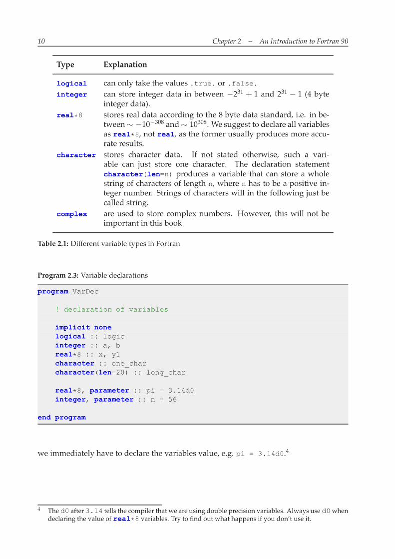
Variables are used to store data during the execution of the program. Table 2.1 summa-rizes the 5 data types Fortran knows. Declaring the type of a variable at the beginningof a program is not compulsory per se. Nevertheless, Fortan implicitly declares all vari-ables that are used in the executable code as integer. This can cause severe problemswhen we run our program and forget to declare one variable that, for example, shouldbe of real*8 type. To prevent Fortran from implicit variable declaration and make dec-laration statements compulsory for any variable, we suggest to always use the statementimplicit none at the beginning of the declarative program part, see Program 2.2. Hav-ing specified implicit none, the compiler will tell us which variables are not yet de-clared and throw an error message during the compilation step.3
Program 2.3 shows some examples of variable declarations. The interpretation of thefirst declaration statements should be clear from the above explanations. In addition tospecifying the type of a variable, we can also make it a parameter like in the last twostatements of the program. This basically tells the compiler that the value of a variableshould be fixed at a certain level and not be changed anymore. Specifying a parameter,
3 Verify this by running Program 2.2 and commenting out the linewhereinput is declared. In the outputwindow of Plato 3 there now will appear an error message when you try to execute the program.
10 Chapter 2 – An Introduction to Fortran 90
Type Explanation
logical can only take the values .true. or .false.integer can store integer data in between −231 + 1 and 231 − 1 (4 byte
integer data).real*8 stores real data according to the 8 byte data standard, i.e. in be-
tween∼ −10−308 and∼ 10308. We suggest to declare all variablesas real*8, not real, as the former usually produces more accu-rate results.
character stores character data. If not stated otherwise, such a vari-able can just store one character. The declaration statementcharacter(len=n) produces a variable that can store a wholestring of characters of length n, where n has to be a positive in-teger number. Strings of characters will in the following just becalled string.
complex are used to store complex numbers. However, this will not beimportant in this book
Table 2.1: Different variable types in Fortran
Program 2.3: Variable declarations
program VarDec
! declaration of variables
implicit nonelogical :: logicinteger :: a, breal*8 :: x, y1character :: one_charcharacter(len=20) :: long_char
real*8, parameter :: pi = 3.14d0integer, parameter :: n = 56
end program
we immediately have to declare the variables value, e.g. pi = 3.14d0.4
4 The d0 after3.14 tells the compiler that we are using double precision variables. Always use d0whendeclaring the value of real*8 variables. Try to find out what happens if you don’t use it.
2.2. Imperative Fortran programs 11
2.2.3 The basics of imperative programming
After having declared the necessary variables, one obviously wants to work with them.The first thing we would like to do is giving values to those variables and display thesevalues on the console.
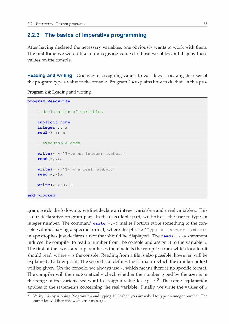
Reading and writing One way of assigning values to variables is making the user ofthe program type a value to the console. Program 2.4 explains how to do that. In this pro-
Program 2.4: Reading and writing
program ReadWrite
! declaration of variables
implicit noneinteger :: areal*8 :: x
! executable code
write(*,*)’Type an integer number:’read(*,*)a
write(*,*)’Type a real number:’read(*,*)x
write(*,*)a, x
end program
gram, we do the following: we first declare an integer variable a and a real variable x. Thisis our declarative program part. In the executable part, we first ask the user to type aninteger number. The command write(*,*) makes Fortran write something to the con-sole without having a specific format, where the phrase ’Type an integer number:’
in apostrophes just declares a text that should be displayed. The read(*,*)a statementinduces the compiler to read a number from the console and assign it to the variable a.The first of the two stars in parentheses thereby tells the compiler from which location itshould read, where * is the console. Reading from a file is also possible, however, will beexplained at a later point. The second star defines the format in which the number or textwill be given. On the console, we always use *, which means there is no specific format.The compiler will then automatically check whether the number typed by the user is inthe range of the variable we want to assign a value to, e.g. a.5 The same explanationapplies to the statements concerning the real variable. Finally, we write the values of a
5 Verify this by running Program 2.4 and typing 12.5 when you are asked to type an integer number. Thecompiler will then throw an error message.
12 Chapter 2 – An Introduction to Fortran 90
and x to the console. Note that we can write several variables at once by just separatingthem with a comma. The same applies to the read statement.
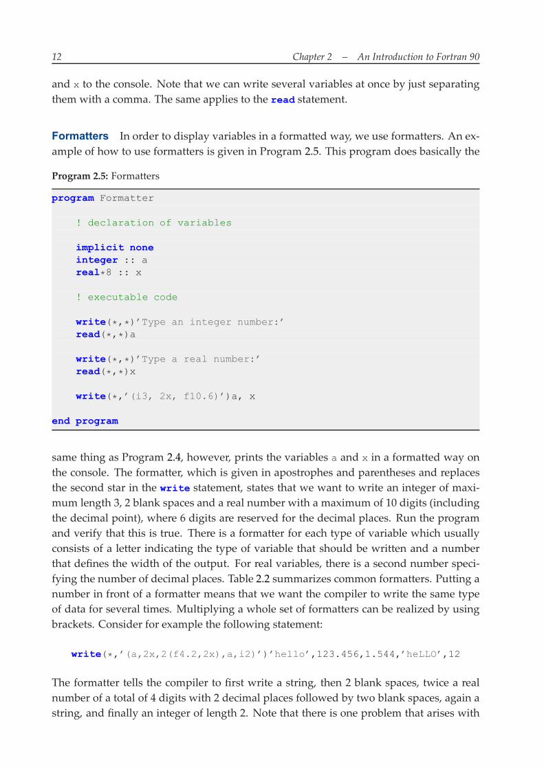
Formatters In order to display variables in a formatted way, we use formatters. An ex-ample of how to use formatters is given in Program 2.5. This program does basically the
Program 2.5: Formatters
program Formatter
! declaration of variables
implicit noneinteger :: areal*8 :: x
! executable code
write(*,*)’Type an integer number:’read(*,*)a
write(*,*)’Type a real number:’read(*,*)x
write(*,’(i3, 2x, f10.6)’)a, x
end program
same thing as Program 2.4, however, prints the variables a and x in a formatted way onthe console. The formatter, which is given in apostrophes and parentheses and replacesthe second star in the write statement, states that we want to write an integer of maxi-mum length 3, 2 blank spaces and a real number with a maximum of 10 digits (includingthe decimal point), where 6 digits are reserved for the decimal places. Run the programand verify that this is true. There is a formatter for each type of variable which usuallyconsists of a letter indicating the type of variable that should be written and a numberthat defines the width of the output. For real variables, there is a second number speci-fying the number of decimal places. Table 2.2 summarizes common formatters. Putting anumber in front of a formatter means that we want the compiler to write the same typeof data for several times. Multiplying a whole set of formatters can be realized by usingbrackets. Consider for example the following statement:
write(*,’(a,2x,2(f4.2,2x),a,i2)’)’hello’,123.456,1.544,’heLLO’,12
The formatter tells the compiler to first write a string, then 2 blank spaces, twice a realnumber of a total of 4 digits with 2 decimal places followed by two blank spaces, again astring, and finally an integer of length 2. Note that there is one problem that arises with
2.2. Imperative Fortran programs 13
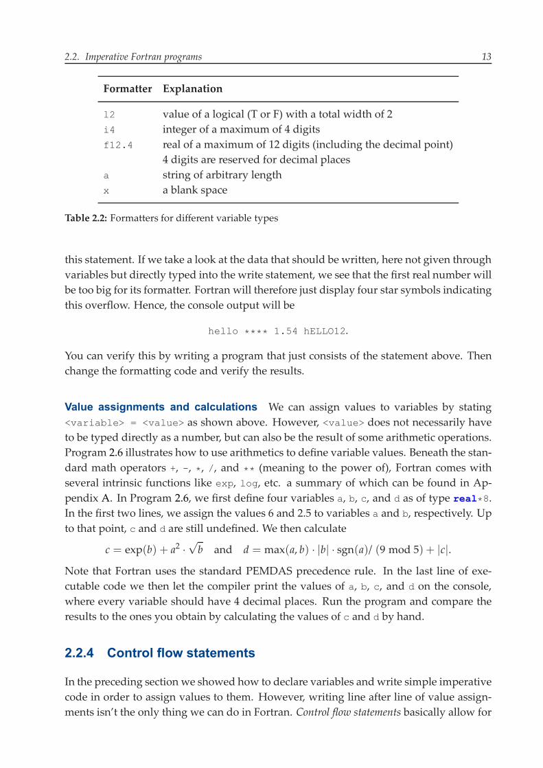
Formatter Explanation
l2 value of a logical (T or F) with a total width of 2i4 integer of a maximum of 4 digitsf12.4 real of a maximum of 12 digits (including the decimal point)
4 digits are reserved for decimal placesa string of arbitrary lengthx a blank space
Table 2.2: Formatters for different variable types
this statement. If we take a look at the data that should be written, here not given throughvariables but directly typed into the write statement, we see that the first real number willbe too big for its formatter. Fortran will therefore just display four star symbols indicatingthis overflow. Hence, the console output will be
hello **** 1.54 hELLO12.
You can verify this by writing a program that just consists of the statement above. Thenchange the formatting code and verify the results.
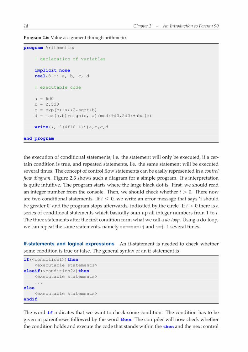
Value assignments and calculations We can assign values to variables by stating<variable> = <value> as shown above. However, <value> does not necessarily haveto be typed directly as a number, but can also be the result of some arithmetic operations.Program 2.6 illustrates how to use arithmetics to define variable values. Beneath the stan-dard math operators +, -, *, /, and ** (meaning to the power of), Fortran comes withseveral intrinsic functions like exp, log, etc. a summary of which can be found in Ap-pendix A. In Program 2.6, we first define four variables a, b, c, and d as of type real*8.In the first two lines, we assign the values 6 and 2.5 to variables a and b, respectively. Upto that point, c and d are still undefined. We then calculate
c = exp(b) + a2 ·√b and d = max(a, b) · |b| · sgn(a)/ (9 mod 5) + |c|.
Note that Fortran uses the standard PEMDAS precedence rule. In the last line of exe-cutable code we then let the compiler print the values of a, b, c, and d on the console,where every variable should have 4 decimal places. Run the program and compare theresults to the ones you obtain by calculating the values of c and d by hand.
2.2.4 Control flow statements
In the preceding section we showed how to declare variables andwrite simple imperativecode in order to assign values to them. However, writing line after line of value assign-ments isn’t the only thing we can do in Fortran. Control flow statements basically allow for
14 Chapter 2 – An Introduction to Fortran 90
Program 2.6: Value assignment through arithmetics
program Arithmetics
! declaration of variables
implicit nonereal*8 :: a, b, c, d
! executable code
a = 6d0b = 2.5d0c = exp(b)+a**2*sqrt(b)d = max(a,b)*sign(b, a)/mod(9d0,5d0)+abs(c)
write(*, ’(4f10.4)’)a,b,c,d
end program
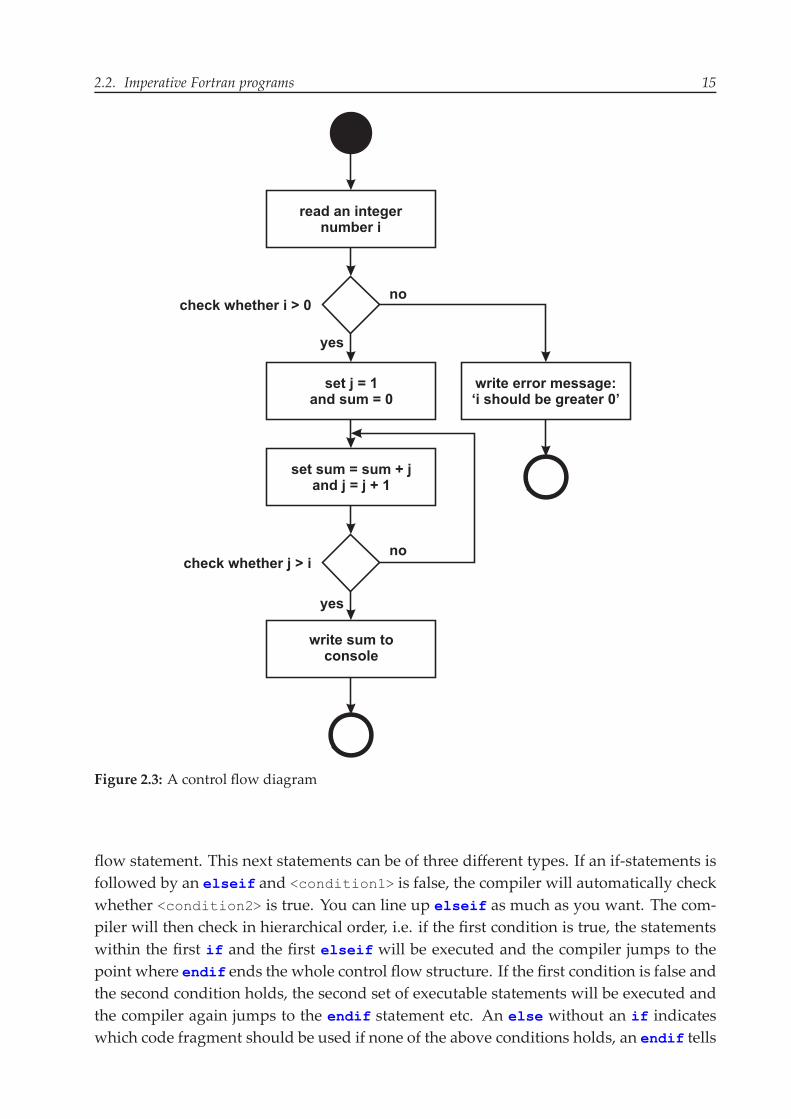
the execution of conditional statements, i.e. the statement will only be executed, if a cer-tain condition is true, and repeated statements, i.e. the same statement will be executedseveral times. The concept of control flow statements can be easily represented in a controlflow diagram. Figure 2.3 shows such a diagram for a simple program. It’s interpretationis quite intuitive. The program starts where the large black dot is. First, we should readan integer number from the console. Then, we should check whether i > 0. There noware two conditional statements. If i ≤ 0, we write an error message that says ’i shouldbe greater 0’ and the program stops afterwards, indicated by the circle. If i > 0 there is aseries of conditional statements which basically sum up all integer numbers from 1 to i.The three statements after the first condition formwhat we call a do-loop. Using a do-loop,we can repeat the same statements, namely sum=sum+j and j=j+1 several times.
If-statements and logical expressions An if-statement is needed to check whethersome condition is true or false. The general syntax of an if-statement is
if(<condition1>)then<executable statements>
elseif(<condition2>)then<executable statements>...
else<executable statements>
endif
The word if indicates that we want to check some condition. The condition has to begiven in parentheses followed by the word then. The compiler will now check whetherthe condition holds and execute the code that stands within the then and the next control
2.2. Imperative Fortran programs 15
read an integernumber i
check whether i > 0
yes
no
write error message:‘i should be greater 0’
set j = 1sum = 0and
set sum = sum + jand j = j + 1
check whether j > ino
yes
write sum toconsole
Figure 2.3: A control flow diagram
flow statement. This next statements can be of three different types. If an if-statements isfollowed by an elseif and <condition1> is false, the compiler will automatically checkwhether <condition2> is true. You can line up elseif as much as you want. The com-piler will then check in hierarchical order, i.e. if the first condition is true, the statementswithin the first if and the first elseif will be executed and the compiler jumps to thepoint where endif ends the whole control flow structure. If the first condition is false andthe second condition holds, the second set of executable statements will be executed andthe compiler again jumps to the endif statement etc. An else without an if indicateswhich code fragment should be used if none of the above conditions holds, an endif tells
16 Chapter 2 – An Introduction to Fortran 90
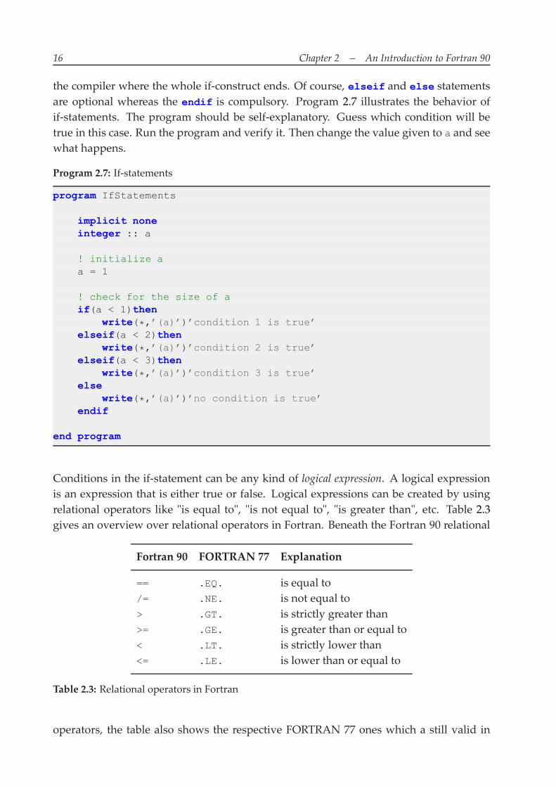
the compiler where the whole if-construct ends. Of course, elseif and else statementsare optional whereas the endif is compulsory. Program 2.7 illustrates the behavior ofif-statements. The program should be self-explanatory. Guess which condition will betrue in this case. Run the program and verify it. Then change the value given to a and seewhat happens.
Program 2.7: If-statements
program IfStatements
implicit noneinteger :: a
! initialize aa = 1
! check for the size of aif(a < 1)then
write(*,’(a)’)’condition 1 is true’elseif(a < 2)then
write(*,’(a)’)’condition 2 is true’elseif(a < 3)then
write(*,’(a)’)’condition 3 is true’else
write(*,’(a)’)’no condition is true’endif
end program
Conditions in the if-statement can be any kind of logical expression. A logical expressionis an expression that is either true or false. Logical expressions can be created by usingrelational operators like "is equal to", "is not equal to", "is greater than", etc. Table 2.3gives an overview over relational operators in Fortran. Beneath the Fortran 90 relational
Fortran 90 FORTRAN 77 Explanation
== .EQ. is equal to/= .NE. is not equal to> .GT. is strictly greater than>= .GE. is greater than or equal to< .LT. is strictly lower than<= .LE. is lower than or equal to
Table 2.3: Relational operators in Fortran
operators, the table also shows the respective FORTRAN 77 ones which a still valid in
2.2. Imperative Fortran programs 17
Fortran 90. In the following, we will only use the Fortran 90 commands. Nevertheless,you can find the old operators in a lot of code especially in older textbooks. An exam-ple for a logical expression is a + b <= c. Note that relational operators bind less thanmathematical ones, i.e. the compiler will first evaluate all mathematical parts of logicalstatements and then the relational ones. Let e.g. a = 3, b = 5 and c = 6. The logicalexpression will therefore be evaluated in the following way:
a + b <= c ⇒ 3 + 5 <= 6 ⇒ 8 <= 6 ⇒ .false.
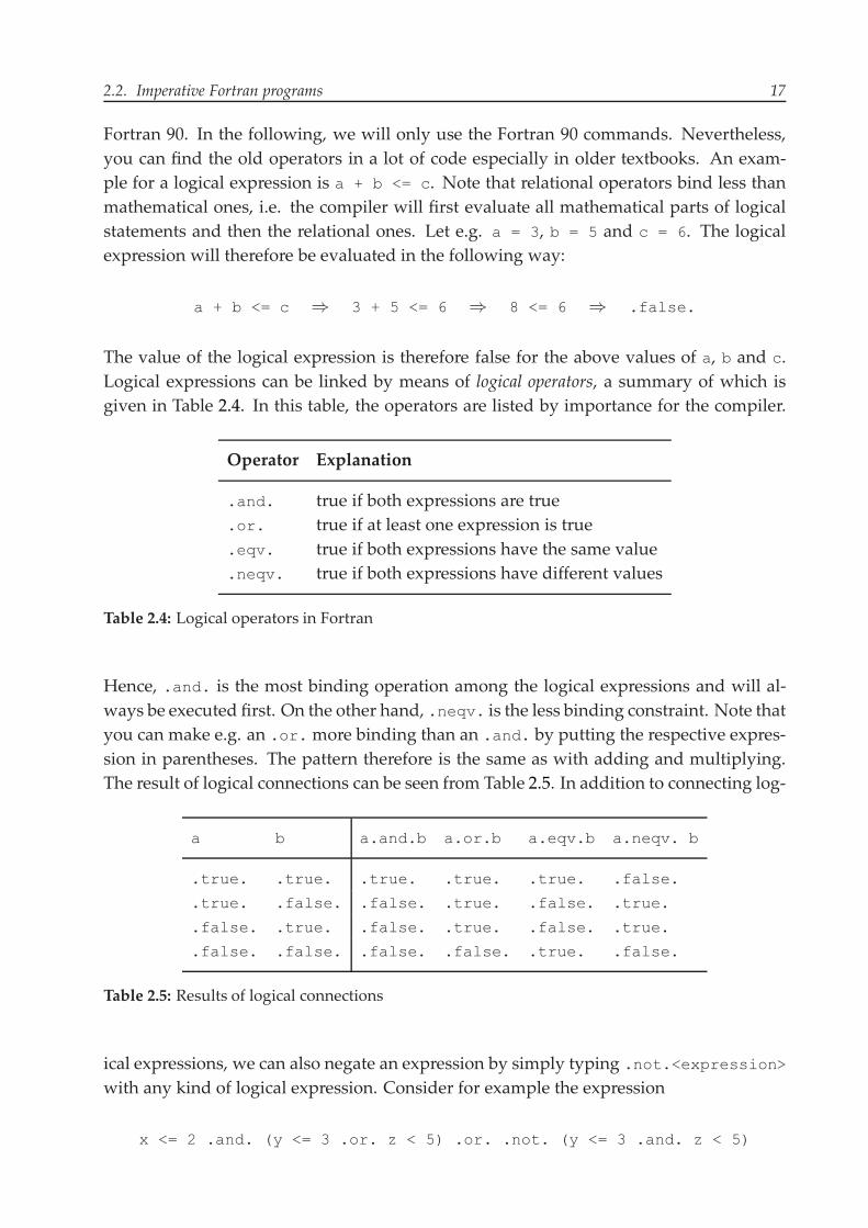
The value of the logical expression is therefore false for the above values of a, b and c.Logical expressions can be linked by means of logical operators, a summary of which isgiven in Table 2.4. In this table, the operators are listed by importance for the compiler.
Operator Explanation
.and. true if both expressions are true
.or. true if at least one expression is true
.eqv. true if both expressions have the same value
.neqv. true if both expressions have different values
Table 2.4: Logical operators in Fortran
Hence, .and. is the most binding operation among the logical expressions and will al-ways be executed first. On the other hand, .neqv. is the less binding constraint. Note thatyou can make e.g. an .or.more binding than an .and. by putting the respective expres-sion in parentheses. The pattern therefore is the same as with adding and multiplying.The result of logical connections can be seen from Table 2.5. In addition to connecting log-
a b a.and.b a.or.b a.eqv.b a.neqv. b
.true. .true. .true. .true. .true. .false.
.true. .false. .false. .true. .false. .true.
.false. .true. .false. .true. .false. .true.
.false. .false. .false. .false. .true. .false.
Table 2.5: Results of logical connections
ical expressions, we can also negate an expression by simply typing .not.<expression>with any kind of logical expression. Consider for example the expression
x <= 2 .and. (y <= 3 .or. z < 5) .or. .not. (y <= 3 .and. z < 5)
18 Chapter 2 – An Introduction to Fortran 90
x <= 2 .and. (y <= 3 .or. z < 5) .or. .not. (y <= 3 .and. z < 5)
4 <= 2 .and. (6 <= 3 .or. 8 < 5) .or. .not. (6 <= 3 .and. 8 < 5)
.false. .and. (.false. .or. .false.) .or. .not. (.false. .and. .false.)
.false. .and. .false. .or. .not. .false.
.false. .or. .true.
.true.
x=4 y=6 z=8 y=6 z=8
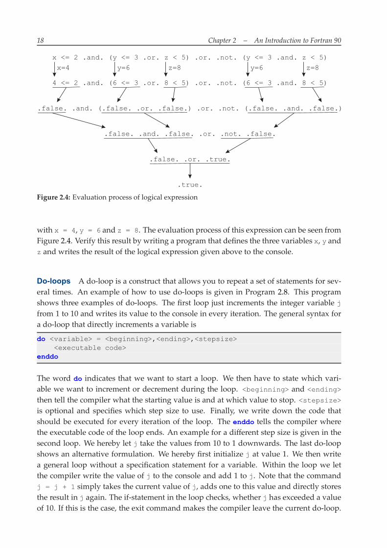
Figure 2.4: Evaluation process of logical expression
with x = 4, y = 6 and z = 8. The evaluation process of this expression can be seen fromFigure 2.4. Verify this result by writing a program that defines the three variables x, y andz and writes the result of the logical expression given above to the console.
Do-loops A do-loop is a construct that allows you to repeat a set of statements for sev-eral times. An example of how to use do-loops is given in Program 2.8. This programshows three examples of do-loops. The first loop just increments the integer variable jfrom 1 to 10 and writes its value to the console in every iteration. The general syntax fora do-loop that directly increments a variable is
do <variable> = <beginning>,<ending>,<stepsize><executable code>
enddo
The word do indicates that we want to start a loop. We then have to state which vari-able we want to increment or decrement during the loop. <beginning> and <ending>
then tell the compiler what the starting value is and at which value to stop. <stepsize>is optional and specifies which step size to use. Finally, we write down the code thatshould be executed for every iteration of the loop. The enddo tells the compiler wherethe executable code of the loop ends. An example for a different step size is given in thesecond loop. We hereby let j take the values from 10 to 1 downwards. The last do-loopshows an alternative formulation. We hereby first initialize j at value 1. We then writea general loop without a specification statement for a variable. Within the loop we letthe compiler write the value of j to the console and add 1 to j. Note that the commandj = j + 1 simply takes the current value of j, adds one to this value and directly storesthe result in j again. The if-statement in the loop checks, whether j has exceeded a valueof 10. If this is the case, the exit command makes the compiler leave the current do-loop.
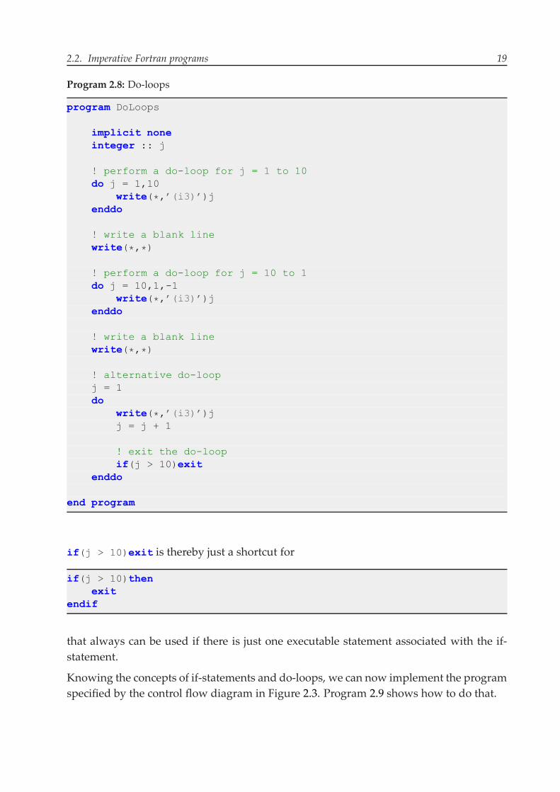
2.2. Imperative Fortran programs 19
Program 2.8: Do-loops
program DoLoops
implicit noneinteger :: j
! perform a do-loop for j = 1 to 10do j = 1,10
write(*,’(i3)’)jenddo
! write a blank linewrite(*,*)
! perform a do-loop for j = 10 to 1do j = 10,1,-1
write(*,’(i3)’)jenddo
! write a blank linewrite(*,*)
! alternative do-loopj = 1do
write(*,’(i3)’)jj = j + 1
! exit the do-loopif(j > 10)exit
enddo
end program
if(j > 10)exit is thereby just a shortcut for
if(j > 10)thenexit
endif
that always can be used if there is just one executable statement associated with the if-statement.
Knowing the concepts of if-statements and do-loops, we can now implement the programspecified by the control flow diagram in Figure 2.3. Program 2.9 shows how to do that.
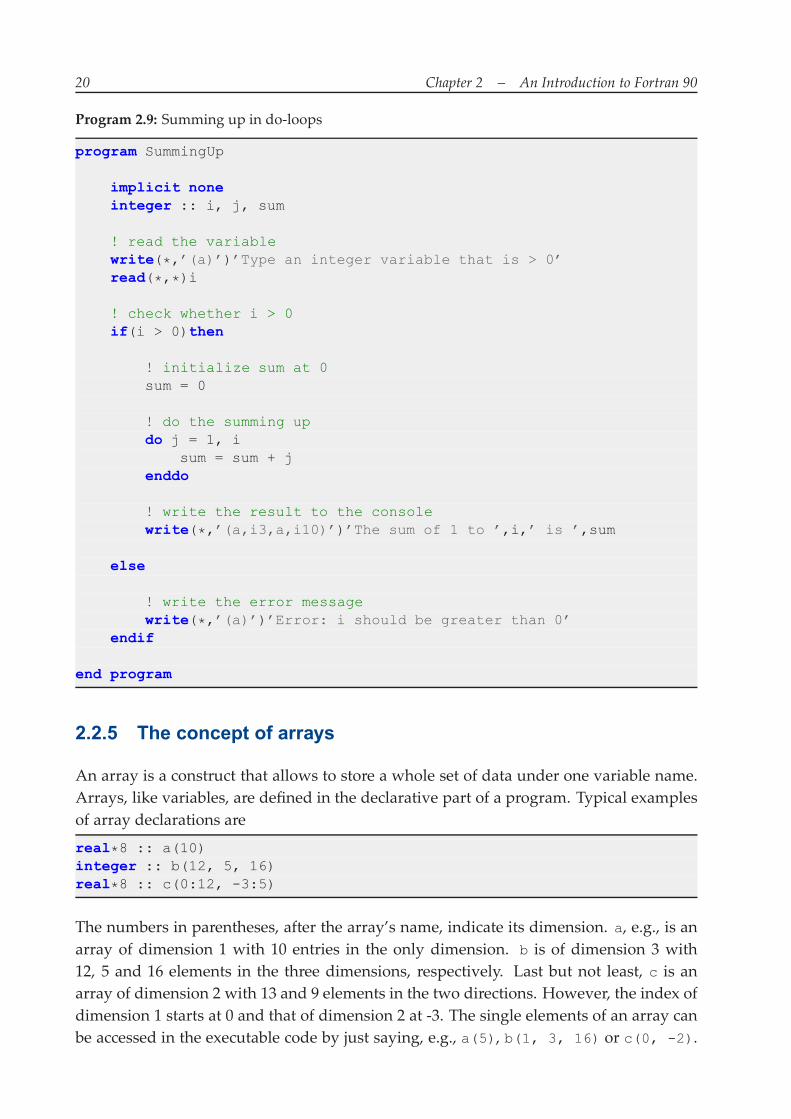
20 Chapter 2 – An Introduction to Fortran 90
Program 2.9: Summing up in do-loops
program SummingUp
implicit noneinteger :: i, j, sum
! read the variablewrite(*,’(a)’)’Type an integer variable that is > 0’read(*,*)i
! check whether i > 0if(i > 0)then
! initialize sum at 0sum = 0
! do the summing updo j = 1, i
sum = sum + jenddo
! write the result to the consolewrite(*,’(a,i3,a,i10)’)’The sum of 1 to ’,i,’ is ’,sum
else
! write the error messagewrite(*,’(a)’)’Error: i should be greater than 0’
endif
end program
2.2.5 The concept of arrays
An array is a construct that allows to store a whole set of data under one variable name.Arrays, like variables, are defined in the declarative part of a program. Typical examplesof array declarations are
real*8 :: a(10)integer :: b(12, 5, 16)real*8 :: c(0:12, -3:5)
The numbers in parentheses, after the array’s name, indicate its dimension. a, e.g., is anarray of dimension 1 with 10 entries in the only dimension. b is of dimension 3 with12, 5 and 16 elements in the three dimensions, respectively. Last but not least, c is anarray of dimension 2 with 13 and 9 elements in the two directions. However, the index ofdimension 1 starts at 0 and that of dimension 2 at -3. The single elements of an array canbe accessed in the executable code by just saying, e.g., a(5), b(1, 3, 16) or c(0, -2).
2.2. Imperative Fortran programs 21
The statement b(1, 3, 16) then returns the value of the array at positions 1, 3, and 16in the three dimensions, respectively. Note that, if not defined otherwise, an array’s indexalways starts with 1. In the case of c, however, we made the array index start with 0 andgo up to 12 in the first dimension, which means a total size of 13.
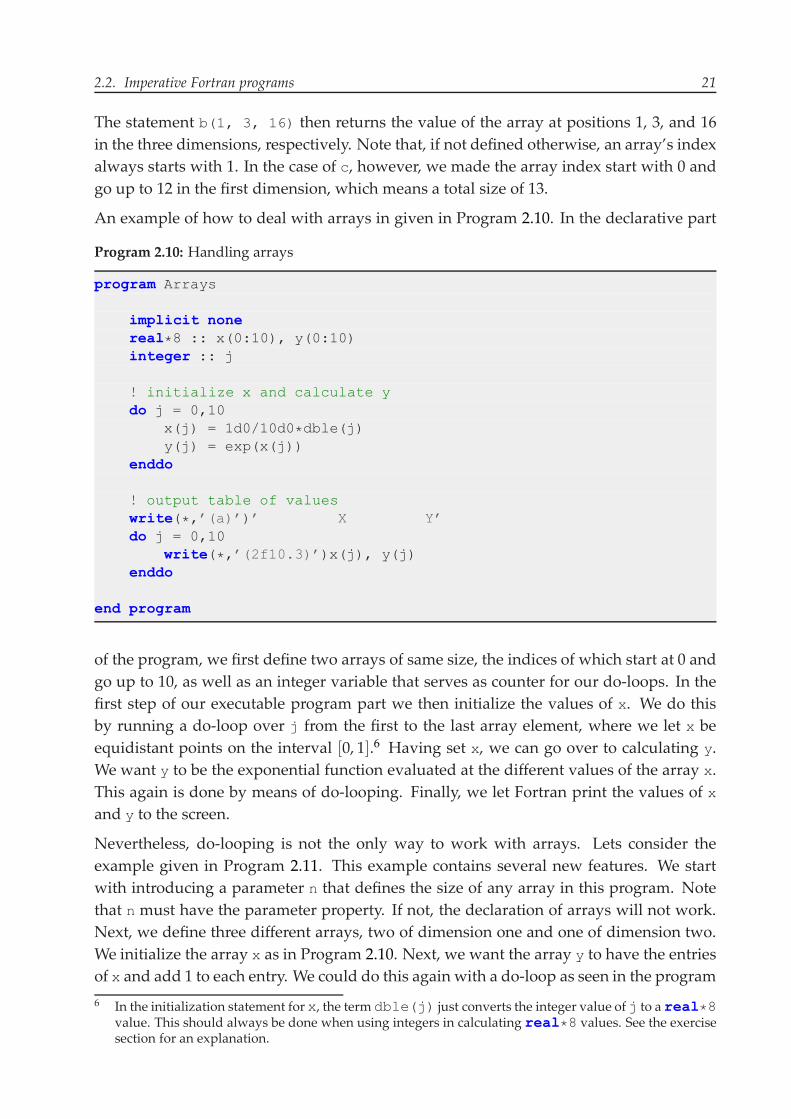
An example of how to deal with arrays in given in Program 2.10. In the declarative part
Program 2.10: Handling arrays
program Arrays
implicit nonereal*8 :: x(0:10), y(0:10)integer :: j
! initialize x and calculate ydo j = 0,10
x(j) = 1d0/10d0*dble(j)y(j) = exp(x(j))
enddo
! output table of valueswrite(*,’(a)’)’ X Y’do j = 0,10
write(*,’(2f10.3)’)x(j), y(j)enddo
end program
of the program, we first define two arrays of same size, the indices of which start at 0 andgo up to 10, as well as an integer variable that serves as counter for our do-loops. In thefirst step of our executable program part we then initialize the values of x. We do thisby running a do-loop over j from the first to the last array element, where we let x beequidistant points on the interval [0, 1].6 Having set x, we can go over to calculating y.We want y to be the exponential function evaluated at the different values of the array x.This again is done by means of do-looping. Finally, we let Fortran print the values of xand y to the screen.
Nevertheless, do-looping is not the only way to work with arrays. Lets consider theexample given in Program 2.11. This example contains several new features. We startwith introducing a parameter n that defines the size of any array in this program. Notethat n must have the parameter property. If not, the declaration of arrays will not work.Next, we define three different arrays, two of dimension one and one of dimension two.We initialize the array x as in Program 2.10. Next, we want the array y to have the entriesof x and add 1 to each entry. We could do this again with a do-loop as seen in the program
6 In the initialization statement for x, the term dble(j) just converts the integer value of j to a real*8value. This should always be done when using integers in calculating real*8 values. See the exercisesection for an explanation.
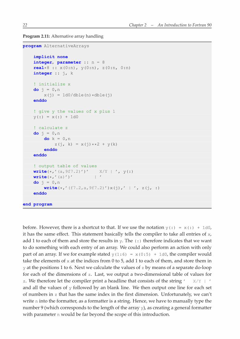
22 Chapter 2 – An Introduction to Fortran 90
Program 2.11: Alternative array handling
program AlternativeArrays
implicit noneinteger, parameter :: n = 8real*8 :: x(0:n), y(0:n), z(0:n, 0:n)integer :: j, k
! initialize xdo j = 0,n
x(j) = 1d0/dble(n)*dble(j)enddo
! give y the values of x plus 1y(:) = x(:) + 1d0
! calculate zdo j = 0,n
do k = 0,nz(j, k) = x(j)**2 + y(k)
enddoenddo
! output table of valueswrite(*,’(a,9f7.2)’)’ X/Y | ’, y(:)write(*,’(a)’)’ | ’do j = 0,n
write(*,’(f7.2,a,9f7.2)’)x(j),’ | ’, z(j, :)enddo
end program
before. However, there is a shortcut to that. If we use the notation y(:) = x(:) + 1d0,it has the same effect. This statement basically tells the compiler to take all entries of x,add 1 to each of them and store the results in y. The (:) therefore indicates that we wantto do something with each entry of an array. We could also perform an action with onlypart of an array. If we for example stated y(1:6) = x(0:5) + 1d0, the compiler wouldtake the elements of x at the indices from 0 to 5, add 1 to each of them, and store them iny at the positions 1 to 6. Next we calculate the values of z by means of a separate do-loopfor each of the dimensions of z. Last, we output a two-dimensional table of values forz. We therefore let the compiler print a headline that consists of the string ’ X/Y | ’
and all the values of y followed by an blank line. We then output one line for each setof numbers in z that has the same index in the first dimension. Unfortunately, we can’twrite n into the formatter, as a formatter is a string. Hence, we have to manually type thenumber 9 (which corresponds to the length of the array y), as creating a general formatterwith parameter nwould be far beyond the scope of this introduction.
2.3. Subroutines and functions 23
2.3 Subroutines and functions
Subroutines and functions can be used to store code that is frequently used within oneprogram. While a subroutine just executes some imperative code, a function is a constructthat, like a function in maths, receives some input value and calculates a return value.
Subroutines Program 2.12 demonstrates how to use subroutines in a Fortran program.Subroutines, as well as functions, are defined outside of the main program. We declare a
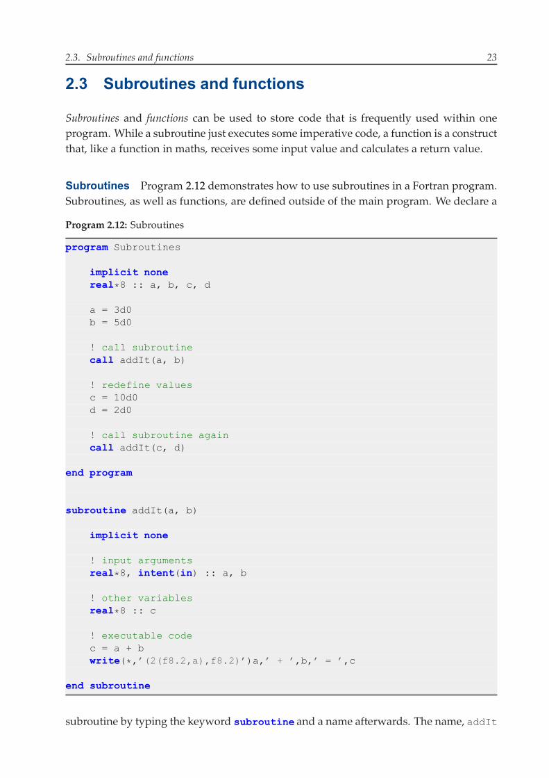
Program 2.12: Subroutines
program Subroutines
implicit nonereal*8 :: a, b, c, d
a = 3d0b = 5d0
! call subroutinecall addIt(a, b)
! redefine valuesc = 10d0d = 2d0
! call subroutine againcall addIt(c, d)
end program
subroutine addIt(a, b)
implicit none
! input argumentsreal*8, intent(in) :: a, b
! other variablesreal*8 :: c
! executable codec = a + bwrite(*,’(2(f8.2,a),f8.2)’)a,’ + ’,b,’ = ’,c
end subroutine
subroutine by typing the keyword subroutine and a name afterwards. The name, addIt
24 Chapter 2 – An Introduction to Fortran 90
in the case of Program 2.12, must follow the Fortran naming conventions as describedin Section 2.1.4 and must neither correspond to the program name nor any name of avariable declared in the main program. After having specified the name, we can tellFortran which communication variables the subroutine receives from the main program.7
These communication variables are the only interface that links the main program to thesubroutine. All other variables declared in the main program can not be used. In ourcase, we specified two input variables, a and b, the sum of which will be calculated andwritten to the console. Note that communication variables do not have to be simple inputarguments per se. If we pass on a variable and change its value within the subroutine,the change will also be adopted by the main program. The structure of a subroutine isnow pretty much the same as that of a main program. We first have a declarative part inwhich we define all variables used in the subroutine, including communication variables.In addition, we can regulate whether our communication variables should be of input oroutput type. This is done via an intent statement. If a variable’s intent is in, we are notallowed to change its value throughout the subroutine.8 If the intent is out, the variablemust be given a value within the subroutine. Specifying inout has the same effect asnot declaring any intent. After having declared all variables, the executable part of oursubroutine specifies what to do with them. We can use any kind of executable statementswe know from our main programs.
When it comes to using a subroutine in a main program, we use the keyword call fol-lowed by the name of the subroutine that should be called.9 In addition, we have to spec-ify which variables of the main program to pass on to the subroutine, where the numberand type of variables must be exactly the same as those specified in the subroutine’s dec-laration. In our case, we use the subroutine with different variables twice. Note thatwe declared the variables a, b, and c in the main program as well as in the subroutine.This usually is no problem, as the subroutine does not know about the variable namesdeclared in the main program. It just takes the communication variables as given andworks with its own variable declarations.
Functions Functions are a bit more difficult to use. Program 2.13 shows an example.Declaring a function is very similar to declaring a subroutine. However, in addition tospecifying the type and intent of communications variables, we also have to state thefunction’s return value. This is done using a type declaration with the function’s name.The name will therefore serve as a regular variable throughout the executable part of thefunction. The value given to this variable finally is the return value of the function, whichin our example corresponds to the sum of a and b. In the main program, things are a bitmore complicated. The problem is to tell the main program that there is a function out
7 You do not need to specify any communication variable. Just type empty parentheses in this case.8 Verify this by trying to change the value of a in the above subroutine. When compiling, there now
should be an error in the output window saying that this is not allowed.9 Subroutines do not necessarily have to be called by a main program, but can also be used by other
subroutines.
2.3. Subroutines and functions 25
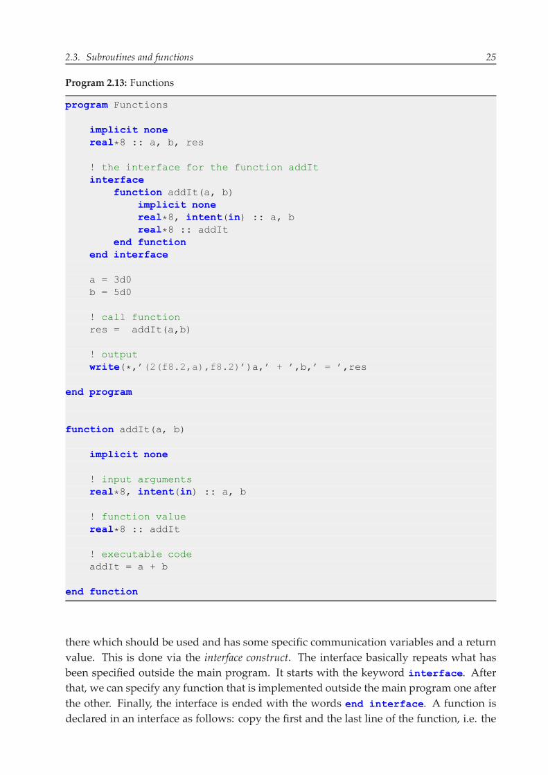
Program 2.13: Functions
program Functions
implicit nonereal*8 :: a, b, res
! the interface for the function addItinterface
function addIt(a, b)implicit nonereal*8, intent(in) :: a, breal*8 :: addIt
end functionend interface
a = 3d0b = 5d0
! call functionres = addIt(a,b)
! outputwrite(*,’(2(f8.2,a),f8.2)’)a,’ + ’,b,’ = ’,res
end program
function addIt(a, b)
implicit none
! input argumentsreal*8, intent(in) :: a, b
! function valuereal*8 :: addIt
! executable codeaddIt = a + b
end function
there which should be used and has some specific communication variables and a returnvalue. This is done via the interface construct. The interface basically repeats what hasbeen specified outside the main program. It starts with the keyword interface. Afterthat, we can specify any function that is implemented outside the main program one afterthe other. Finally, the interface is ended with the words end interface. A function isdeclared in an interface as follows: copy the first and the last line of the function, i.e. the
26 Chapter 2 – An Introduction to Fortran 90
part that starts with function and the end function statement. Then just copy all dec-larations of communication variables and the function type declaration to the interface,as we did in Program 2.13. You do not need to copy local variable declaration statement,i.e. the declaration of variables that are only used within the function.
Having specified the function through our interface construct, we now can use it in ourmain program. As a function has a return value, we do not call it via a call statementlike a subroutine, but assign the return value directly to a variable, res in our case. resnow contains our function value, i.e. the sum of a and b. Finally, we write the result tothe console.
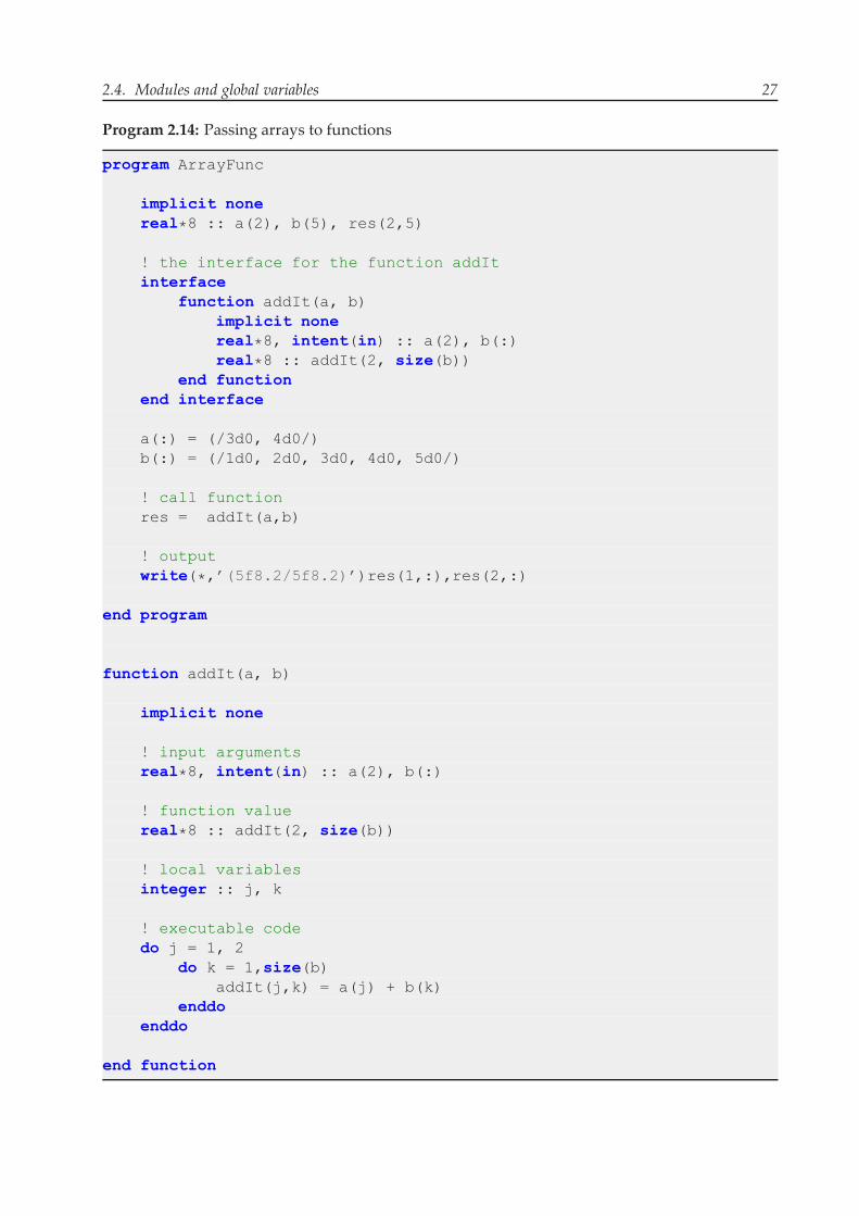
Passing arrays to functions or subroutines Sometimes one would like to pass anarray to a function or subroutine. This can be done in two ways, see Program 2.14. If wetake a look at the function declaration, we see that communication variable a is specifiedlike we would specify a regular array in a main program. The declaration statementtherefore tells the compiler that it should expect an array of dimension 1 and length 2 to bepassed to the function. In the case of b, we used the so-called assumed-shape statement.Typing a : instead of a valid integer number, we allow the length of b to be anything.The compiler therefore will just expect an array of dimension one, but with an arbitrarylength. However, we can refer to b’s length, which will be calculated on-the-fly duringruntime, by typing size(b).10 We consequently define our return value as an array oftwo dimensions, the first of which is of size 2 and the second of the same size as b. Theexecutable code of our function should then be straightforward. The interface is adaptedanalogically.
In the main program, we now specify three arrays. The two input arrays of dimension 1and the array that should store the result of our function. This arraymust have dimension2 with the size of a in dimension 1 and that of b in dimension 2. We then initialize thearrays a and b. There is a shortcut to do this by saying a(:) = (/<values>/), where<values> is just a comma separated list of initialization values. Finally, we can call ourfunction, assign the return value to res, and write the result to the console.
2.4 Modules and global variables
A module is a construct that allows to store frequently used code and variables in a sep-arate location. The code and variables can then be used by different programs.
10 If you declare a multidimensional array, you can refer to the length into any dimension by statingsize(b, <dim>)where <dim> is just an integer number declaring the dimension.
2.4. Modules and global variables 27
Program 2.14: Passing arrays to functions
program ArrayFunc
implicit nonereal*8 :: a(2), b(5), res(2,5)
! the interface for the function addItinterface
function addIt(a, b)implicit nonereal*8, intent(in) :: a(2), b(:)real*8 :: addIt(2, size(b))
end functionend interface
a(:) = (/3d0, 4d0/)b(:) = (/1d0, 2d0, 3d0, 4d0, 5d0/)
! call functionres = addIt(a,b)
! outputwrite(*,’(5f8.2/5f8.2)’)res(1,:),res(2,:)
end program
function addIt(a, b)
implicit none
! input argumentsreal*8, intent(in) :: a(2), b(:)
! function valuereal*8 :: addIt(2, size(b))
! local variablesinteger :: j, k
! executable codedo j = 1, 2
do k = 1,size(b)addIt(j,k) = a(j) + b(k)
enddoenddo
end function
28 Chapter 2 – An Introduction to Fortran 90
2.4.1 Storing code in a module
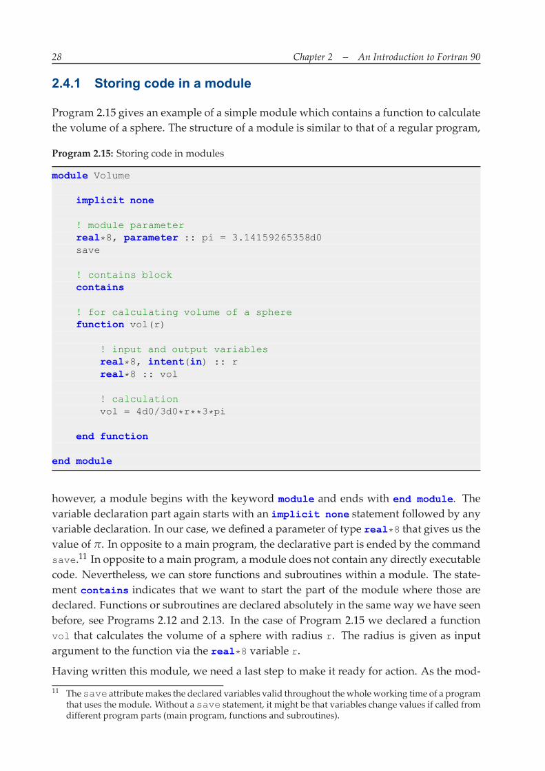
Program 2.15 gives an example of a simple module which contains a function to calculatethe volume of a sphere. The structure of a module is similar to that of a regular program,
Program 2.15: Storing code in modules
module Volume
implicit none
! module parameterreal*8, parameter :: pi = 3.14159265358d0save
! contains blockcontains
! for calculating volume of a spherefunction vol(r)
! input and output variablesreal*8, intent(in) :: rreal*8 :: vol
! calculationvol = 4d0/3d0*r**3*pi
end function
end module
however, a module begins with the keyword module and ends with end module. Thevariable declaration part again starts with an implicit none statement followed by anyvariable declaration. In our case, we defined a parameter of type real*8 that gives us thevalue of π. In opposite to a main program, the declarative part is ended by the commandsave.11 In opposite to a main program, a module does not contain any directly executablecode. Nevertheless, we can store functions and subroutines within a module. The state-ment contains indicates that we want to start the part of the module where those aredeclared. Functions or subroutines are declared absolutely in the same way we have seenbefore, see Programs 2.12 and 2.13. In the case of Program 2.15 we declared a functionvol that calculates the volume of a sphere with radius r. The radius is given as inputargument to the function via the real*8 variable r.
Having written this module, we need a last step to make it ready for action. As the mod-
11 Thesave attributemakes the declared variables valid throughout thewhole working time of a programthat uses the module. Without a save statement, it might be that variables change values if called fromdifferent program parts (main program, functions and subroutines).
2.4. Modules and global variables 29
ule contains no directly executable code, we can’t run it on the console like a regularprogram, but we have to compile it. This is done by clicking the Compile-shortcut sym-bol (in the second line of shortcut symbols the one on the left, see Figure 2.2) or pressingCtrl+F7. Compiling the module, there should appear a message in the output windowsaying "Compilation completed with no errors". Now go to the folder in which you putthe module code, i.e. prog2_15.f90. You will now see two files, prog2_15.mod andprog2_15.obj. The .mod file contains information about the module, its variables andprocedures, whereas the .obj file contains the binary object code of the module that canbe linked to other executable code by the compiler, see Figure 2.1. Note that if you want aprogram to use this module, those two files have to lie in the same folder as the programitself.
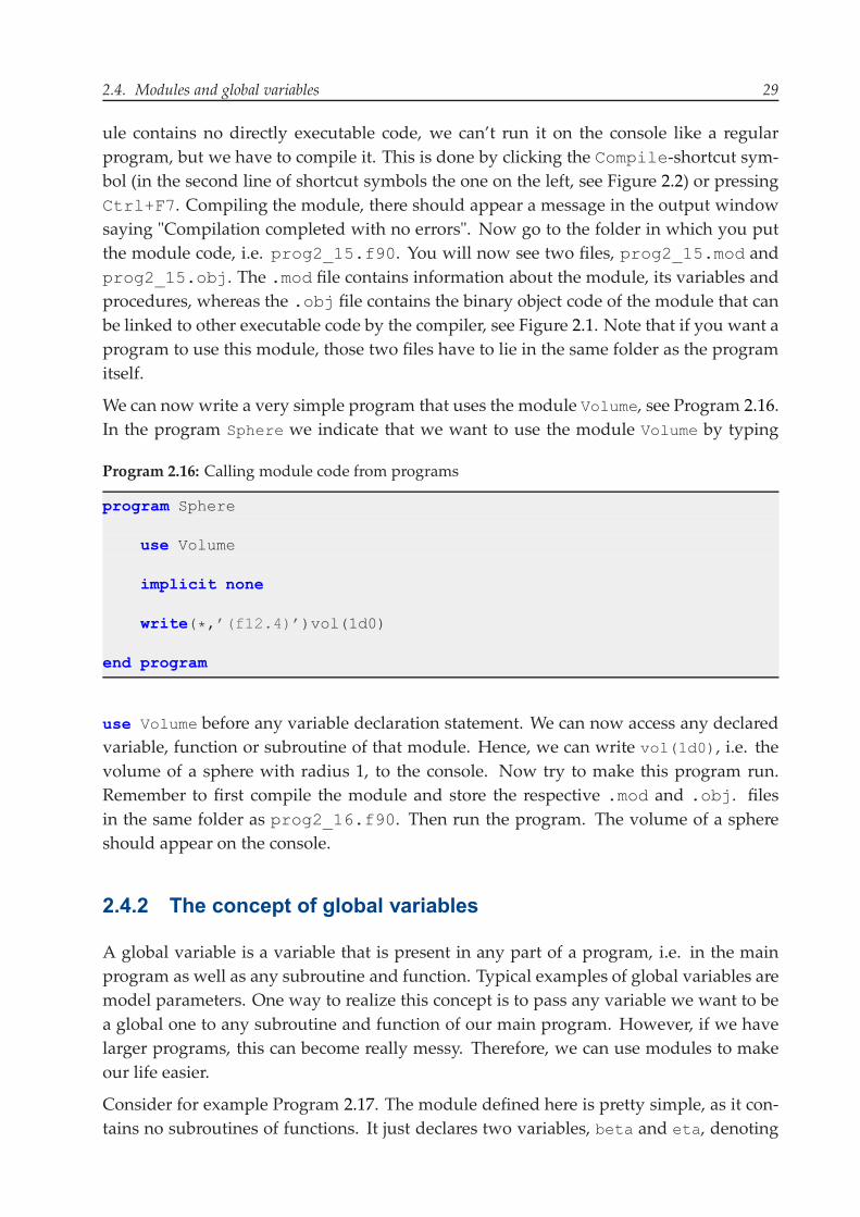
We can now write a very simple program that uses the module Volume, see Program 2.16.In the program Sphere we indicate that we want to use the module Volume by typing
Program 2.16: Calling module code from programs
program Sphere
use Volume
implicit none
write(*,’(f12.4)’)vol(1d0)
end program
use Volume before any variable declaration statement. We can now access any declaredvariable, function or subroutine of that module. Hence, we can write vol(1d0), i.e. thevolume of a sphere with radius 1, to the console. Now try to make this program run.Remember to first compile the module and store the respective .mod and .obj. filesin the same folder as prog2_16.f90. Then run the program. The volume of a sphereshould appear on the console.
2.4.2 The concept of global variables
A global variable is a variable that is present in any part of a program, i.e. in the mainprogram as well as any subroutine and function. Typical examples of global variables aremodel parameters. One way to realize this concept is to pass any variable we want to bea global one to any subroutine and function of our main program. However, if we havelarger programs, this can become really messy. Therefore, we can use modules to makeour life easier.
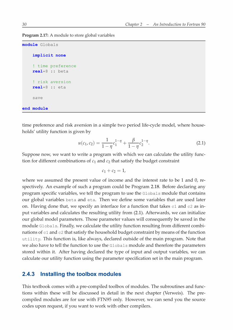
Consider for example Program 2.17. The module defined here is pretty simple, as it con-tains no subroutines of functions. It just declares two variables, beta and eta, denoting
30 Chapter 2 – An Introduction to Fortran 90
Program 2.17: Amodule to store global variables
module Globals
implicit none
! time preferencereal*8 :: beta
! risk aversionreal*8 :: eta
save
end module
time preference and risk aversion in a simple two period life-cycle model, where house-holds’ utility function is given by
u(c1, c2) =1
1− ηc1−η1 +
β
1− ηc1−η2 . (2.1)
Suppose now, we want to write a program with which we can calculate the utility func-tion for different combinations of c1 and c2 that satisfy the budget constraint
c1 + c2 = 1,
where we assumed the present value of income and the interest rate to be 1 and 0, re-spectively. An example of such a program could be Program 2.18. Before declaring anyprogram specific variables, we tell the program to use the Globalsmodule that containsour global variables beta and eta. Then we define some variables that are used lateron. Having done that, we specify an interface for a function that takes c1 and c2 as in-put variables and calculates the resulting utility from (2.1). Afterwards, we can initializeour global model parameters. Those parameter values will consequently be saved in themodule Globals. Finally, we calculate the utility function resulting from different combi-nations of c1 and c2 that satisfy the household budget constraint bymeans of the functionutility. This function is, like always, declared outside of the main program. Note thatwe also have to tell the function to use the Globalsmodule and therefore the parametersstored within it. After having declared the type of input and output variables, we cancalculate our utility function using the parameter specification set in the main program.
2.4.3 Installing the toolbox modules
This textbook comes with a pre-compiled toolbox of modules. The subroutines and func-tions within these will be discussed in detail in the next chapter (Verweis). The pre-compiled modules are for use with FTN95 only. However, we can send you the sourcecodes upon request, if you want to work with other compilers.
2.4. Modules and global variables 31
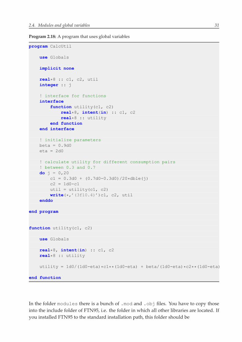
Program 2.18: A program that uses global variables
program CalcUtil
use Globals
implicit none
real*8 :: c1, c2, utilinteger :: j
! interface for functionsinterface
function utility(c1, c2)real*8, intent(in) :: c1, c2real*8 :: utility
end functionend interface
! initialize parametersbeta = 0.9d0eta = 2d0
! calculate utility for different consumption pairs! between 0.3 and 0.7do j = 0,20
c1 = 0.3d0 + (0.7d0-0.3d0)/20*dble(j)c2 = 1d0-c1util = utility(c1, c2)write(*,’(3f10.4)’)c1, c2, util
enddo
end program
function utility(c1, c2)
use Globals
real*8, intent(in) :: c1, c2real*8 :: utility
utility = 1d0/(1d0-eta)*c1**(1d0-eta) + beta/(1d0-eta)*c2**(1d0-eta)
end function
In the folder modules there is a bunch of .mod and .obj files. You have to copy thoseinto the include folder of FTN95, i.e. the folder in which all other libraries are located. Ifyou installed FTN95 to the standard installation path, this folder should be
32 Chapter 2 – An Introduction to Fortran 90
c:\Program Files\Salford Software\FTN95\include,
if not, try to find the folder by searching for FTN95. Copy all .mod and .obj files fromthe modules folder into Fortran’s include folder. If Plato 3 is opened, close and re-openit. The toolbox should now be ready to use.
2.4.4 Plotting graphs with ESPlot
The program ESPlot is a Microsoft® Windows freeware program for engineers and scien-tists provided through the website
http://www.neng.usu.edu/mae/faculty/stevef/prg/ESPlot/index.html
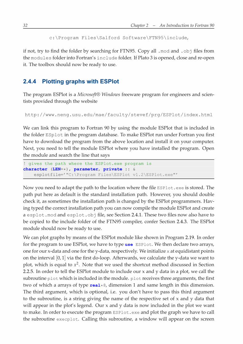
We can link this program to Fortran 90 by using the module ESPlot that is included inthe folder ESplot in the program database. To make ESPlot run under Fortran you firsthave to download the program from the above location and install it on your computer.Next, you need to tell the module ESPlot where you have installed the program. Openthe module and search the line that says
! gives the path where the ESPlot.exe program ischaracter (LEN=*), parameter, private :: &
esplotfile=’"C:\Program Files\ESPlot v1.2\ESPlot.exe"’
Now you need to adapt the path to the location where the file ESPlot.exe is stored. Thepath put here as default is the standard installation path. However, you should doublecheck it, as sometimes the installation path is changed by the ESPlot programmers. Hav-ing typed the correct installation path you can now compile the module ESPlot and createa esplot.mod and esplot.obj file, see Section 2.4.1. These two files now also have tobe copied to the include folder of the FTN95 compiler, confer Section 2.4.3. The ESPlotmodule should now be ready to use.
We can plot graphs by means of the ESPlot module like shown in Program 2.19. In orderfor the program to use ESPlot, we have to type use ESPlot. We then declare two arrays,one for our x-data and one for the y-data, respectively. We initialize x at equidistant pointson the interval [0, 1] via the first do-loop. Afterwards, we calculate the y-data we want toplot, which is equal to x2. Note that we used the shortcut method discussed in Section2.2.5. In order to tell the ESPlot module to include our x and y data in a plot, we call thesubroutine plotwhich is included in themodule. plot receives three arguments, the firsttwo of which a arrays of type real*8, dimension 1 and same length in this dimension.The third argument, which is optional, i.e. you don’t have to pass this third argumentto the subroutine, is a string giving the name of the respective set of x and y data thatwill appear in the plot’s legend. Our x and y data is now included in the plot we wantto make. In order to execute the program ESPlot.exe and plot the graph we have to callthe subroutine execplot. Calling this subroutine, a window will appear on the screen
2.4. Modules and global variables 33
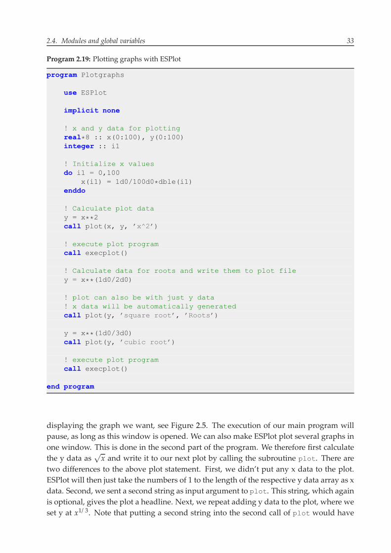
Program 2.19: Plotting graphs with ESPlot
program Plotgraphs
use ESPlot
implicit none
! x and y data for plottingreal*8 :: x(0:100), y(0:100)integer :: i1
! Initialize x valuesdo i1 = 0,100
x(i1) = 1d0/100d0*dble(i1)enddo
! Calculate plot datay = x**2call plot(x, y, ’x^2’)
! execute plot programcall execplot()
! Calculate data for roots and write them to plot filey = x**(1d0/2d0)
! plot can also be with just y data! x data will be automatically generatedcall plot(y, ’square root’, ’Roots’)
y = x**(1d0/3d0)call plot(y, ’cubic root’)
! execute plot programcall execplot()
end program
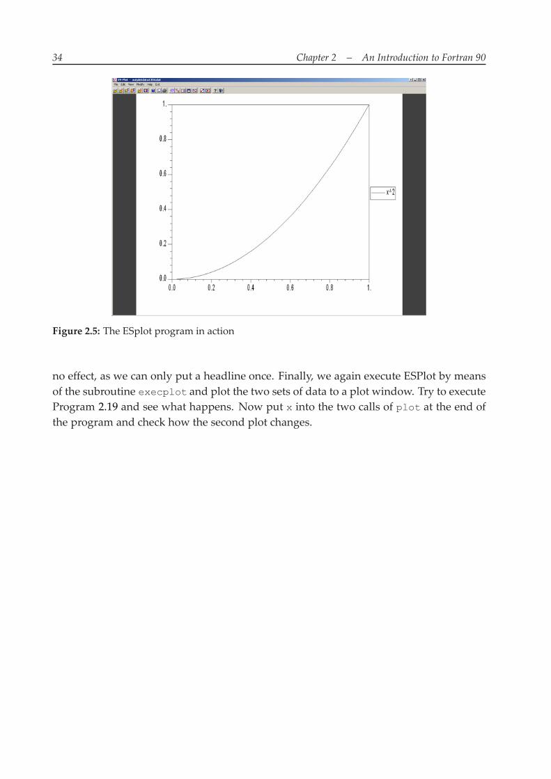
displaying the graph we want, see Figure 2.5. The execution of our main program willpause, as long as this window is opened. We can also make ESPlot plot several graphs inone window. This is done in the second part of the program. We therefore first calculatethe y data as
√x and write it to our next plot by calling the subroutine plot. There are
two differences to the above plot statement. First, we didn’t put any x data to the plot.ESPlot will then just take the numbers of 1 to the length of the respective y data array as xdata. Second, we sent a second string as input argument to plot. This string, which againis optional, gives the plot a headline. Next, we repeat adding y data to the plot, where weset y at x1/ 3. Note that putting a second string into the second call of plot would have
34 Chapter 2 – An Introduction to Fortran 90
Figure 2.5: The ESplot program in action
no effect, as we can only put a headline once. Finally, we again execute ESPlot by meansof the subroutine execplot and plot the two sets of data to a plot window. Try to executeProgram 2.19 and see what happens. Now put x into the two calls of plot at the end ofthe program and check how the second plot changes.