An Introduction to Independent Components Analysis (ICA)

Anish R. Shah, CFA

Northfield Information Services

Anish@northinfo.com

London

Nov 9, 2010

Overview of Talk

• Review principal components

• Introduce independent components

Part I: Principal Components Analysis (PCA)

• At each step, PCA finds the direction that explains the most remaining variation

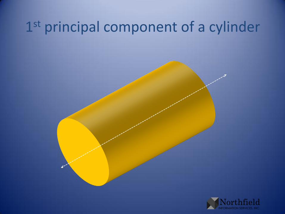
1st principal component of a cylinder

PCA on the Florida Keys

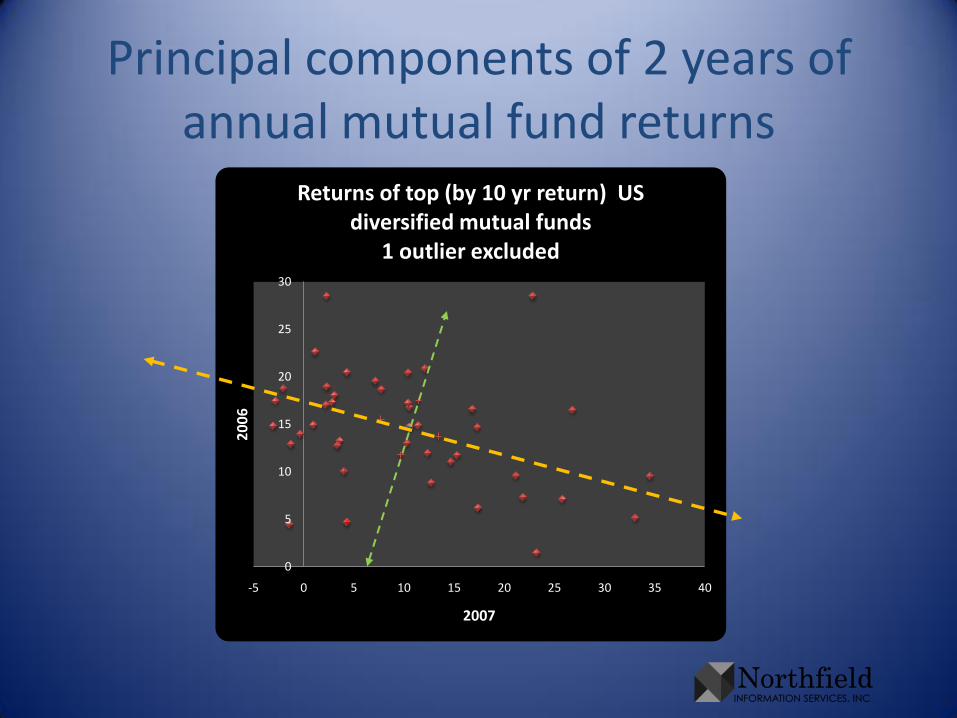
Principal components of 2 years of annual mutual fund returns

0

5

10

15

20

25

30

-5 0 5 10 15 20 25 30 35 40

20

06

2007

Returns of top (by 10 yr return) US diversified mutual funds

1 outlier excluded

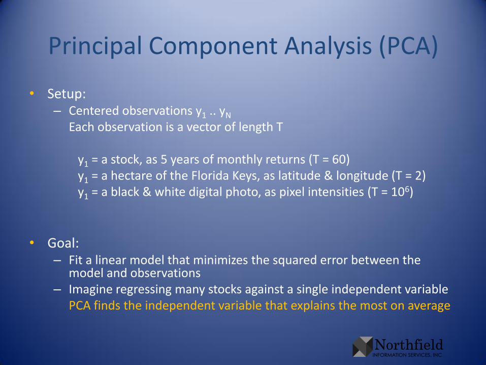
Principal Component Analysis (PCA)

• Setup:– Centered observations y1 .. yN

Each observation is a vector of length T

y1 = a stock, as 5 years of monthly returns (T = 60)y1 = a hectare of the Florida Keys, as latitude & longitude (T = 2)y1 = a black & white digital photo, as pixel intensities (T = 106)

• Goal:– Fit a linear model that minimizes the squared error between the

model and observations– Imagine regressing many stocks against a single independent variable

PCA finds the independent variable that explains the most on average

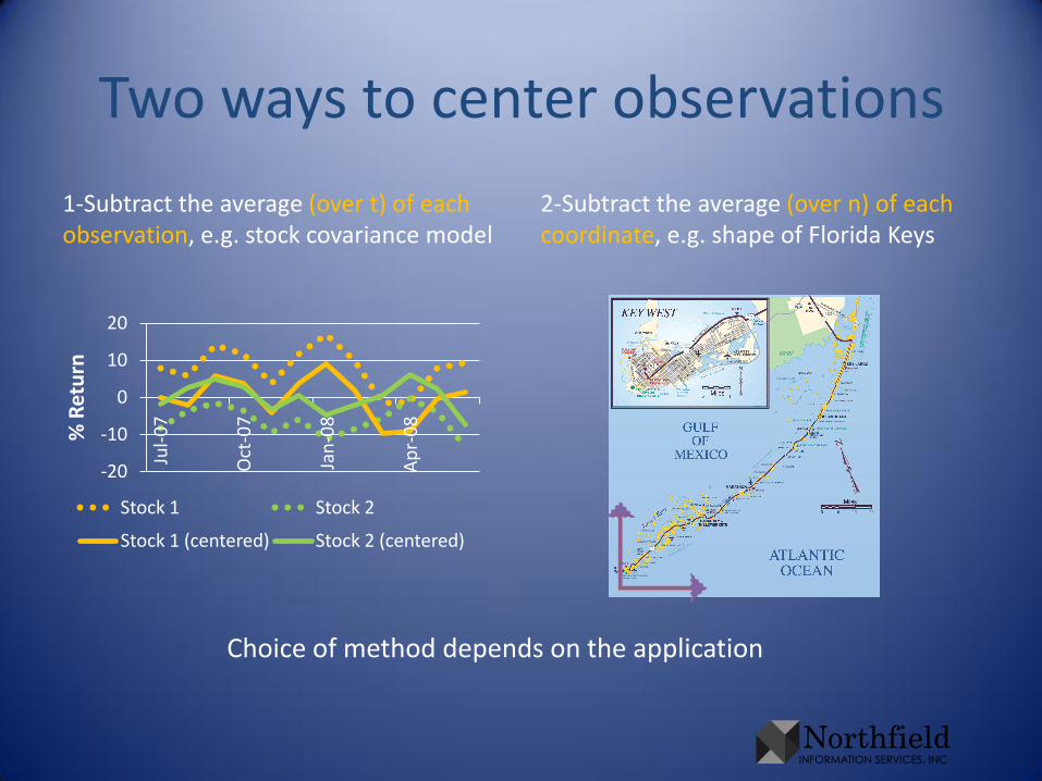
Two ways to center observations

-20

-10

0

10

20

Jul-

07

Oct

-07

Jan

-08

Ap

r-0

8

% R

etu

rn

Stock 1 Stock 2

Stock 1 (centered) Stock 2 (centered)

1-Subtract the average (over t) of each observation, e.g. stock covariance model

2-Subtract the average (over n) of each coordinate, e.g. shape of Florida Keys

Choice of method depends on the application

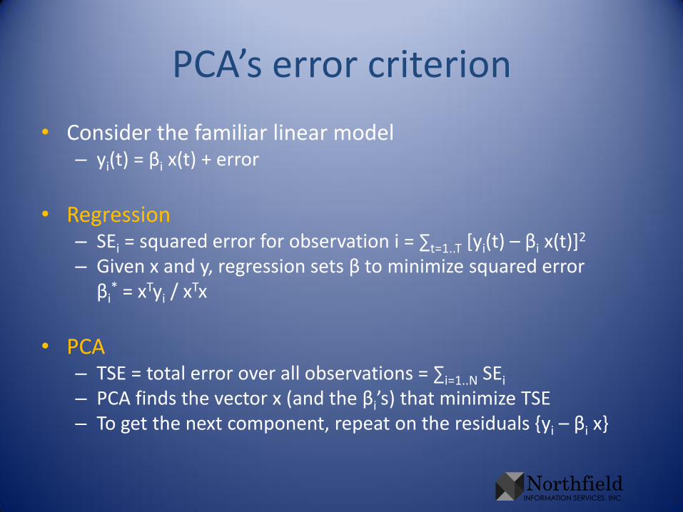
PCA’s error criterion

• Consider the familiar linear model– yi(t) = βi x(t) + error

• Regression– SEi = squared error for observation i = ∑t=1..T [yi(t) – βi x(t)]2

– Given x and y, regression sets β to minimize squared errorβi

* = xTyi / xTx

• PCA– TSE = total error over all observations = ∑i=1..N SEi

– PCA finds the vector x (and the βi’s) that minimize TSE– To get the next component, repeat on the residuals {yi – βi x}

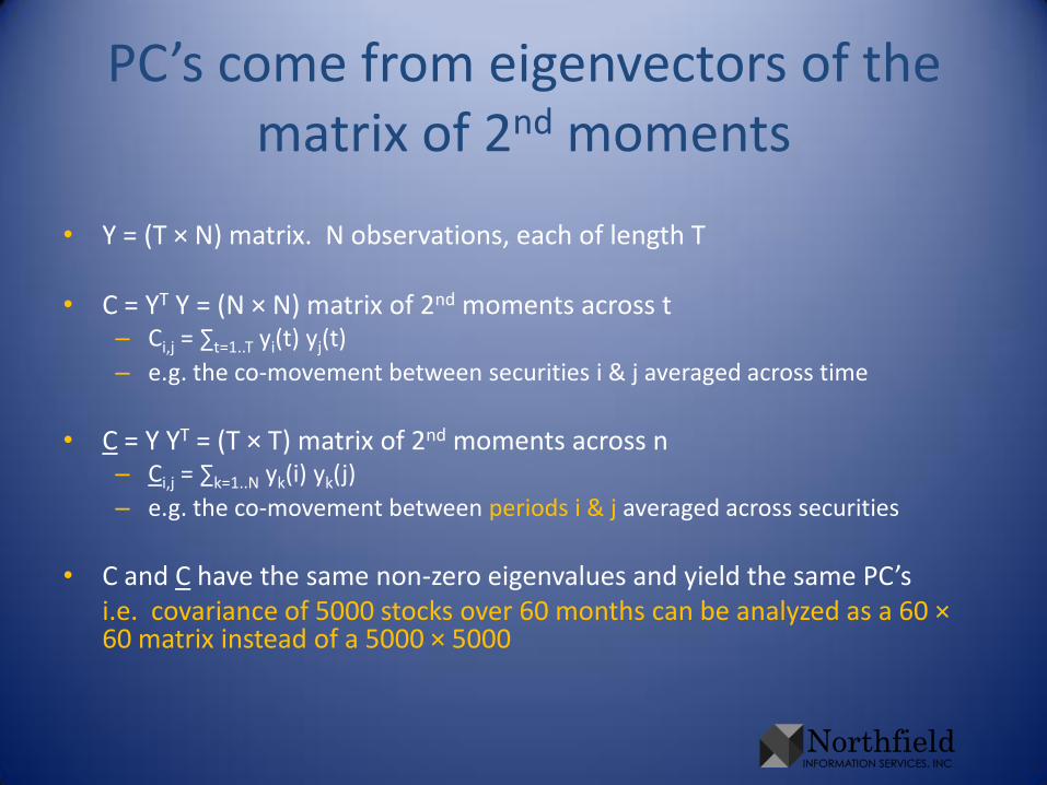
PC’s come from eigenvectors of the matrix of 2nd moments

• Y = (T × N) matrix. N observations, each of length T

• C = YT Y = (N × N) matrix of 2nd moments across t– Ci,j = ∑t=1..T yi(t) yj(t)

– e.g. the co-movement between securities i & j averaged across time

• C = Y YT = (T × T) matrix of 2nd moments across n– Ci,j = ∑k=1..N yk(i) yk(j)

– e.g. the co-movement between periods i & j averaged across securities

• C and C have the same non-zero eigenvalues and yield the same PC’si.e. covariance of 5000 stocks over 60 months can be analyzed as a 60 ×60 matrix instead of a 5000 × 5000

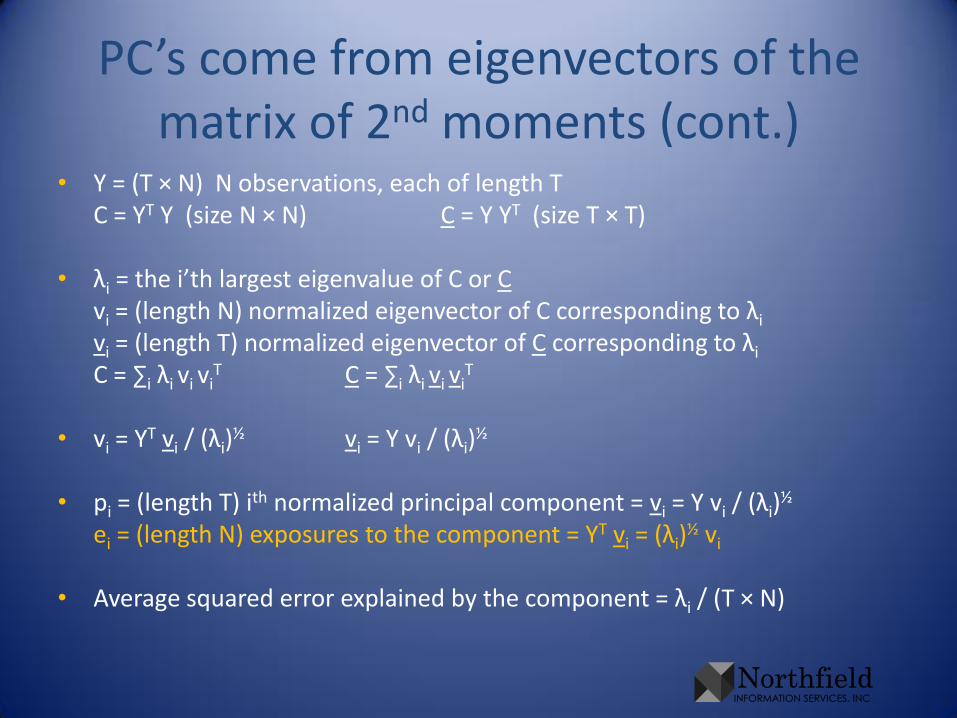
PC’s come from eigenvectors of the matrix of 2nd moments (cont.)

• Y = (T × N) N observations, each of length TC = YT Y (size N × N) C = Y YT (size T × T)

• λi = the i’th largest eigenvalue of C or Cvi = (length N) normalized eigenvector of C corresponding to λi

vi = (length T) normalized eigenvector of C corresponding to λi

C = ∑i λi vi viT C = ∑i λi vi vi

T

• vi = YT vi / (λi)½ vi = Y vi / (λi)

½

• pi = (length T) ith normalized principal component = vi = Y vi / (λi)½

ei = (length N) exposures to the component = YT vi = (λi)½ vi

• Average squared error explained by the component = λi / (T × N)

PCA (cont.)

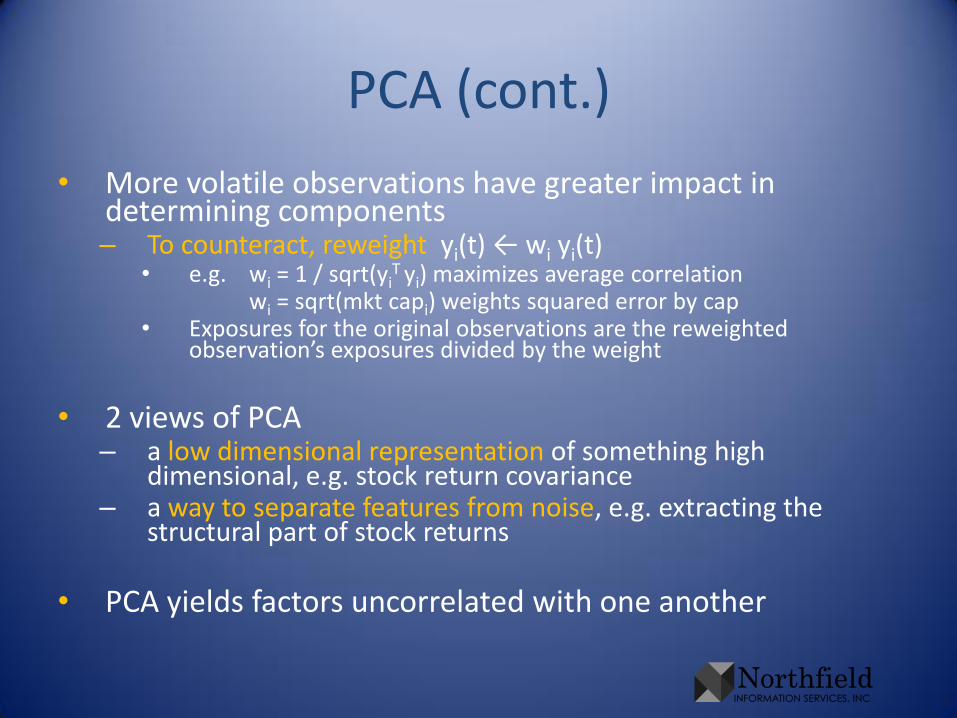
• More volatile observations have greater impact in determining components– To counteract, reweight yi(t) ← wi yi(t)

• e.g. wi = 1 / sqrt(yiT yi) maximizes average correlation

wi = sqrt(mkt capi) weights squared error by cap• Exposures for the original observations are the reweighted

observation’s exposures divided by the weight

• 2 views of PCA– a low dimensional representation of something high

dimensional, e.g. stock return covariance– a way to separate features from noise, e.g. extracting the

structural part of stock returns

• PCA yields factors uncorrelated with one another

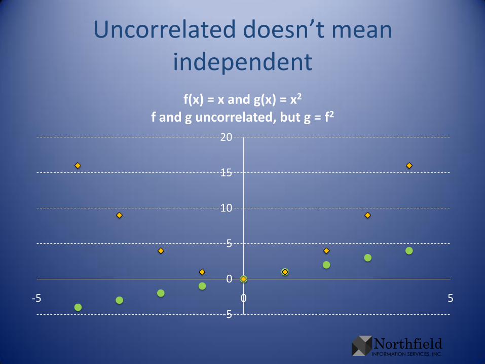
Uncorrelated doesn’t mean independent

-5

0

5

10

15

20

-5 0 5

f(x) = x and g(x) = x2

f and g uncorrelated, but g = f2

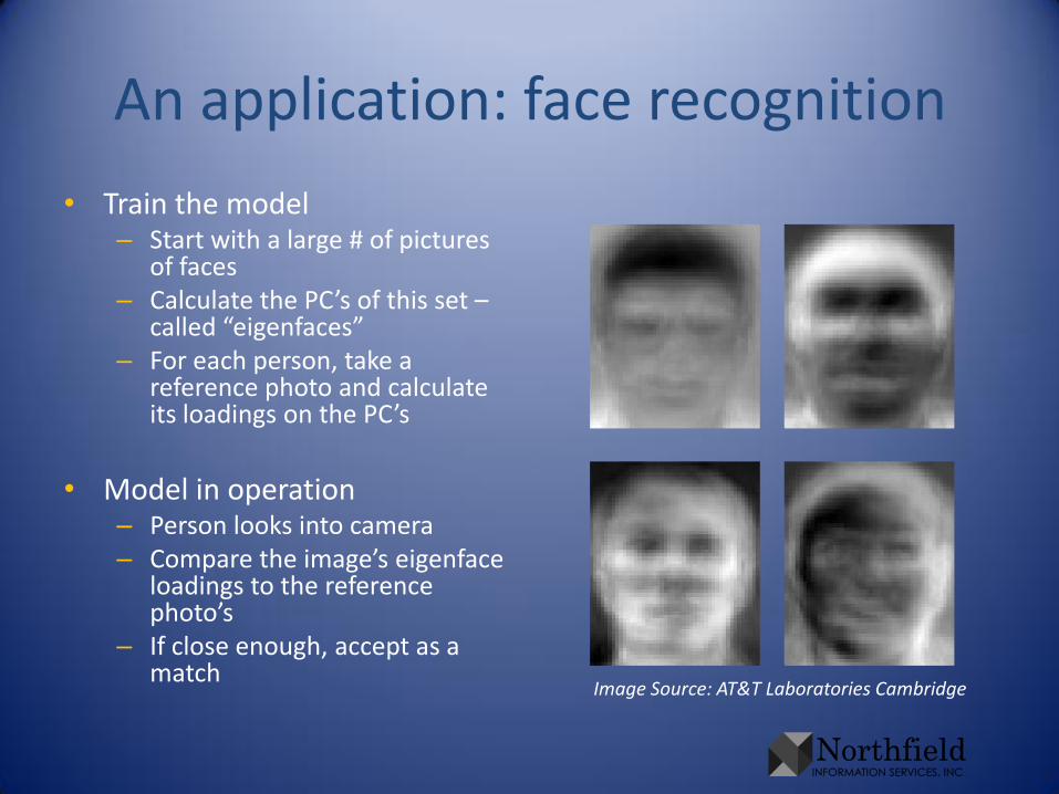
An application: face recognition

• Train the model– Start with a large # of pictures

of faces– Calculate the PC’s of this set –

called “eigenfaces”– For each person, take a

reference photo and calculate its loadings on the PC’s

• Model in operation– Person looks into camera– Compare the image’s eigenface

loadings to the reference photo’s

– If close enough, accept as a match

Image Source: AT&T Laboratories Cambridge

Part II: Independent Components

• Goal: extract the signals driving a process

– Cocktail party problem – separate the sound of several talkers into individual voices

– Stock market returns – extract signals that investors use to price securities, fit predictive model for profit

• Cichocki, Stansell, Leonowicz, & Buck. "Independent variable selection: Application of independent component analysis to forecasting a stock index", Journal of Asset Management, v6(4) Dec 2005

• Back & Weigand. “A first application of independent component analysis to extracting structure from stock returns”, International Journal of Neural Systems, v8(4) Aug 1997

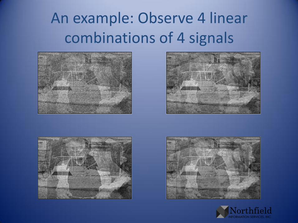
An example: Observe 4 linear combinations of 4 signals

Principal Components

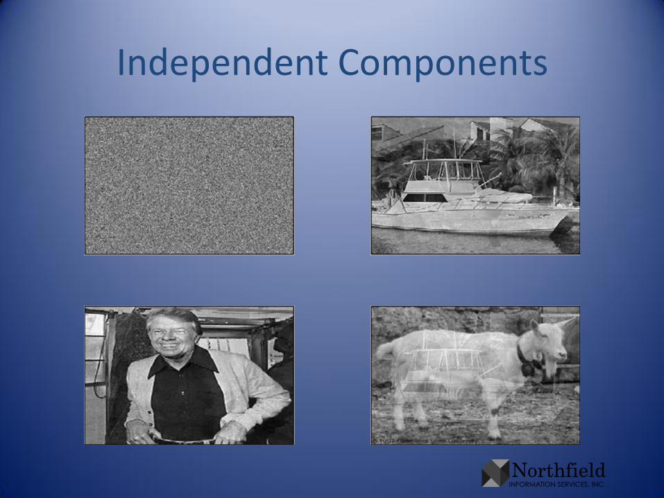
Independent Components

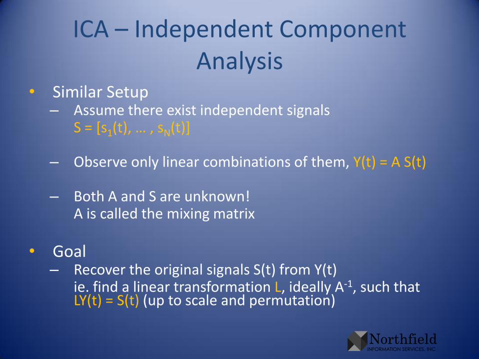
ICA – Independent Component Analysis

• Similar Setup– Assume there exist independent signals

S = [s1(t), … , sN(t)]

– Observe only linear combinations of them, Y(t) = A S(t)

– Both A and S are unknown!A is called the mixing matrix

• Goal– Recover the original signals S(t) from Y(t)

ie. find a linear transformation L, ideally A-1, such that LY(t) = S(t) (up to scale and permutation)

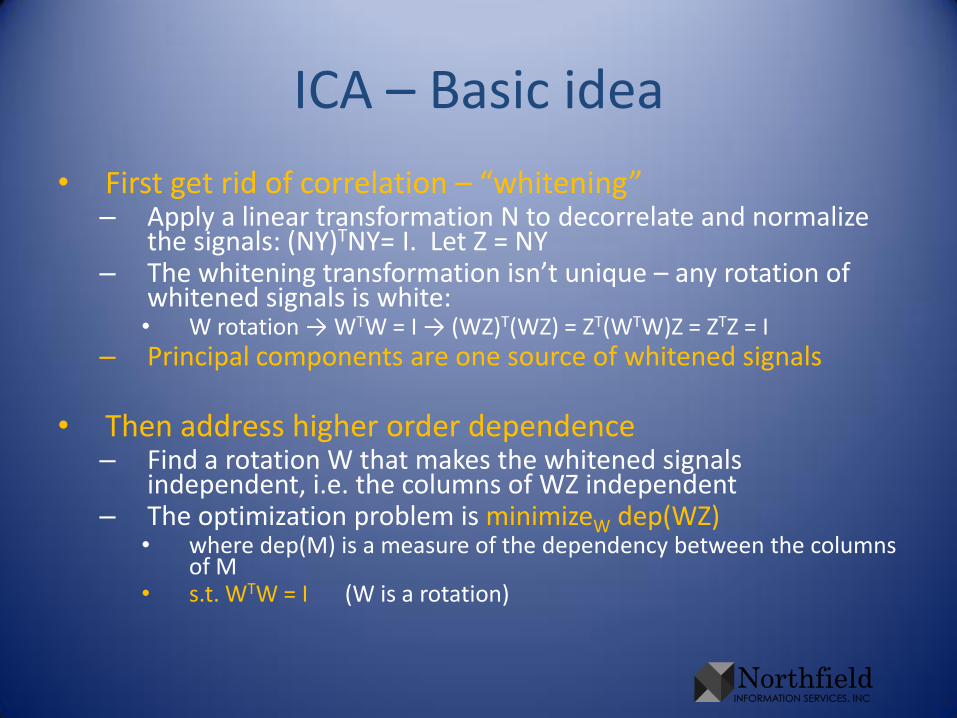
ICA – Basic idea

• First get rid of correlation – “whitening”– Apply a linear transformation N to decorrelate and normalize

the signals: (NY)TNY= I. Let Z = NY– The whitening transformation isn’t unique – any rotation of

whitened signals is white:• W rotation → WTW = I → (WZ)T(WZ) = ZT(WTW)Z = ZTZ = I

– Principal components are one source of whitened signals

• Then address higher order dependence– Find a rotation W that makes the whitened signals

independent, i.e. the columns of WZ independent– The optimization problem is minimizeW dep(WZ)

• where dep(M) is a measure of the dependency between the columns of M

• s.t. WTW = I (W is a rotation)

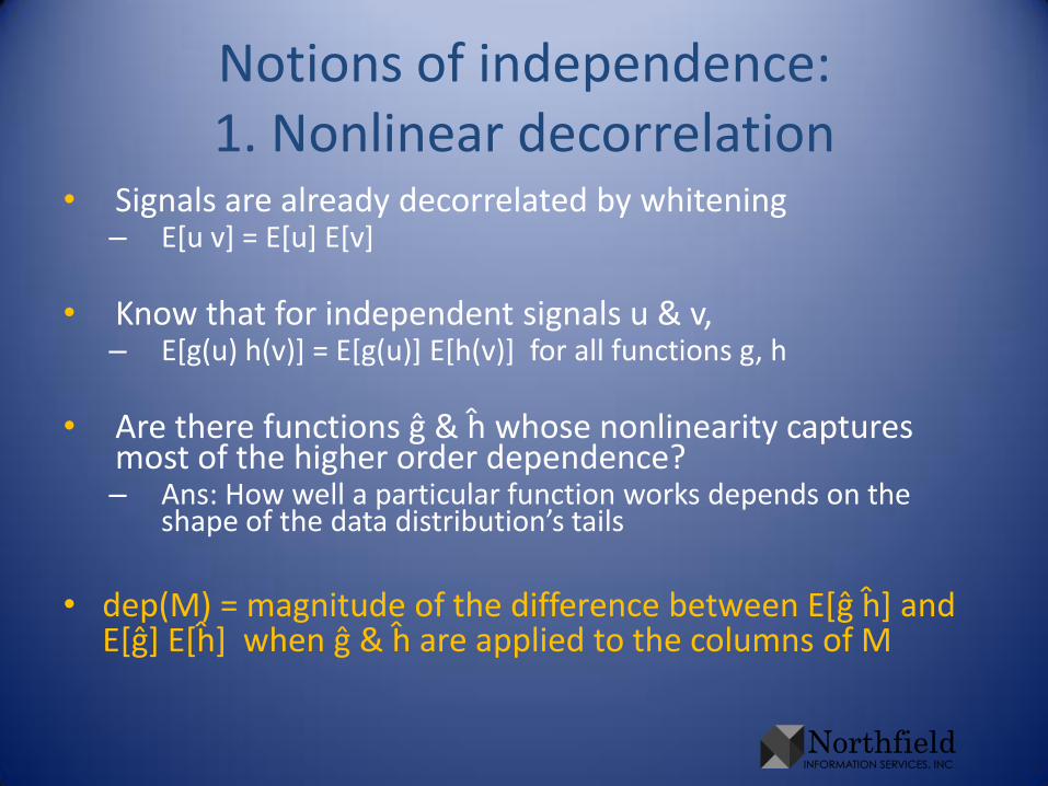
Notions of independence:1. Nonlinear decorrelation

• Signals are already decorrelated by whitening– E[u v] = E[u] E[v]

• Know that for independent signals u & v,– E[g(u) h(v)] = E[g(u)] E[h(v)] for all functions g, h

• Are there functions ĝ & ĥ whose nonlinearity captures most of the higher order dependence?– Ans: How well a particular function works depends on the

shape of the data distribution’s tails

• dep(M) = magnitude of the difference between E[ĝ ĥ] and E[ĝ] E[ĥ] when ĝ & ĥ are applied to the columns of M

Notions of independence:2. Non-Gaussianity

• Model is Y = AS– where the columns of S are independent

• Central limit theorem says adding things together makes them more Gaussian

• Unmixed signals should be less Gaussian

A measure of non-Gaussianity: Kurtosis

• Kurtosis– 4th centered moment / squared variance– A measure of the mass in the distribution’s tails– Highly influenced by outliers– Takes values from 0 to ∞, Gaussian is 3

• Excess Kurtosis = Kurtosis – 3– Takes values from – 3 to ∞, Gaussian is 0– Maximize the absolute value to find non-

Gaussian– dep(M) = -1 × |excess kurtosis of columns of M|

Background: Information theory(Shannon 1948)

• Entropy– H(X) = - ∑ p(x) log p(x)– # of bits needed to encode X

• Differential Entropy (for continuous random variables)– h(X) = - p(x) log p(x) dx– For a given variance, Gaussians maximize differential entropy

• Kullback-Leibler Divergence (Relative Entropy)– D(p||q) = p(x) log [p(x)/q(x)] dx ≥ 0

• Mutual Information– I(X,Y) = D[ p(x,y) || p(x) p(y) ]

= avg # of bits X tells about Y = avg # of bits Y tells about X– I(X,Y) = 0 ↔ X & Y independent

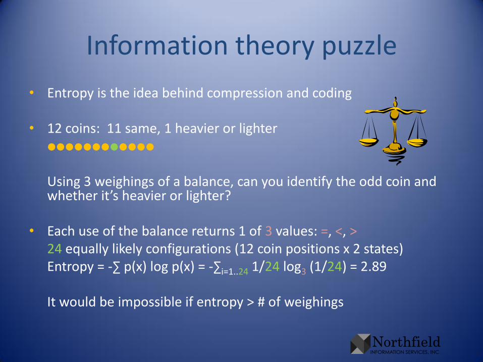
Information theory puzzle

• Entropy is the idea behind compression and coding

• 12 coins: 11 same, 1 heavier or lighter

Using 3 weighings of a balance, can you identify the odd coin and whether it’s heavier or lighter?

• Each use of the balance returns 1 of 3 values: =, <, >24 equally likely configurations (12 coin positions x 2 states)Entropy = -∑ p(x) log p(x) = -∑i=1..24 1/24 log3 (1/24) = 2.89

It would be impossible if entropy > # of weighings

A measure of non-Gaussianity: Negentropy

• Negentropy– Shortfall in entropy relative to a Gaussian with the same

variance– Useful because scale invariant

• To evaluate, need probability distribution– Estimate densities by expansions around a Gaussian density– Cumulant (moment) based (Edgeworth, Gram-Charlier)

• sensitive to outliers

– By non-polynomial functions, e.g. x exp(-x2/2), tanh(x)• more robust, but choice of functions depends on the tails

• Maximize an approximation of negentropy– dep(M) = -1 × |negentropy of columns of M|

Mutual information

• Minimize the mutual information among the signals

– dep(M) = mutual information of columns of M

• After manipulating and constraining the signals to be uncorrelated, minimizing mutual information is maximizing negentropy

Another characterization: Maximum likelihood

• Recall model Y = As– let B = A-1

– p(Y) = |det(B)| ∏i pi(biTY)

• Find demixing matrix B that maximizes the likelihood of the observations Y

• First need an (inexact) model of the p’s, similar to density approximation for negentropy

Connections to human wiring

• ICA can be characterized as sparse coding

– How can signals be represented compactly (each signal loading on a few of the factors) while retaining as much information as possible?

– A neuron codes only a few messages and rarely fires

• Edges are the independent components in pictures of nature

– Our visual system is built to detect edges

Summary

• Incredibly clever and powerful tool for extracting information

• Fundamental – can motivate results from many different starting points

References

• Hyvärinen, A, J Karhunen, and E Oja. Independent Component Analysis. 2001

• Stone, James. Independent Component Analysis: A Tutorial Introduction. 2004

• Bishop, Christopher. Pattern Recognition and Machine Learning. 2007

• Shawe-Taylor, J and N Cristianini. Kernel Methods for Pattern Analysis. 2004