an introduction to langmuir probe diagnostics of...
TRANSCRIPT

An introduction to Langmuir probe
diagnostics of plasmas
Luis Conde
Departamento de Física Aplicada
E.T.S. Ingenieros Aeronáuticos
Universidad Politécnica de Madrid
28040 Madrid, Spain.
May 28, 2011
Abstract
In this short review is introduced the elementary theory of collecting Langmuir probes
in spherical and cylindrical geometries. The classical results for either repelled and at-
tracted charges are deduced and the different approximations and limits of application
are discussed with special insight in laboratory and practical applications. The principles
and operation modes of emissive Langmuir probes are also discussed and also an updated
bibliography is provided for further reading.
Contents
1 Introduction. 3
2 Qualitative description of collecting current voltage curves. 4
3 The simplified theory for collisionless unmagnetized plasmas. 8
3.1 Spherical probe . . . . . . . . . . . . . . . . . . . . . . . . . . . . . . . . . . . . 9
3.1.1 Repelled particles . . . . . . . . . . . . . . . . . . . . . . . . . . . . . . . 10
3.1.2 Attracted particles . . . . . . . . . . . . . . . . . . . . . . . . . . . . . . 12
3.2 Cylindrical probe . . . . . . . . . . . . . . . . . . . . . . . . . . . . . . . . . . . 13
3.2.1 Repelled particles . . . . . . . . . . . . . . . . . . . . . . . . . . . . . . . 14
3.2.2 Attracted particles . . . . . . . . . . . . . . . . . . . . . . . . . . . . . . 15
3.3 Approximations . . . . . . . . . . . . . . . . . . . . . . . . . . . . . . . . . . . . 17
3.3.1 The thin sheath limit . . . . . . . . . . . . . . . . . . . . . . . . . . . . . 17
3.3.2 The thick sheath limit . . . . . . . . . . . . . . . . . . . . . . . . . . . . 18
3.4 The energy distribution function of repelled particles . . . . . . . . . . . . . . . 20
1

Dept. Física. E.T.S.I. Aeronáuticos. Universidad Politécnica de Madrid
4 Interpretation of Langmuir probe data for repelling electrons 21
4.1 The analysis of experimental results . . . . . . . . . . . . . . . . . . . . . . . . 21
5 Emissive Langmuir probes 23
5.1 Floating emissive probe . . . . . . . . . . . . . . . . . . . . . . . . . . . . . . . 24
5.2 The inflection point method . . . . . . . . . . . . . . . . . . . . . . . . . . . . . 26
2
Eur. Master NFEP: Laboratory Project. An introduction to Langmuir probes.
1 Introduction.
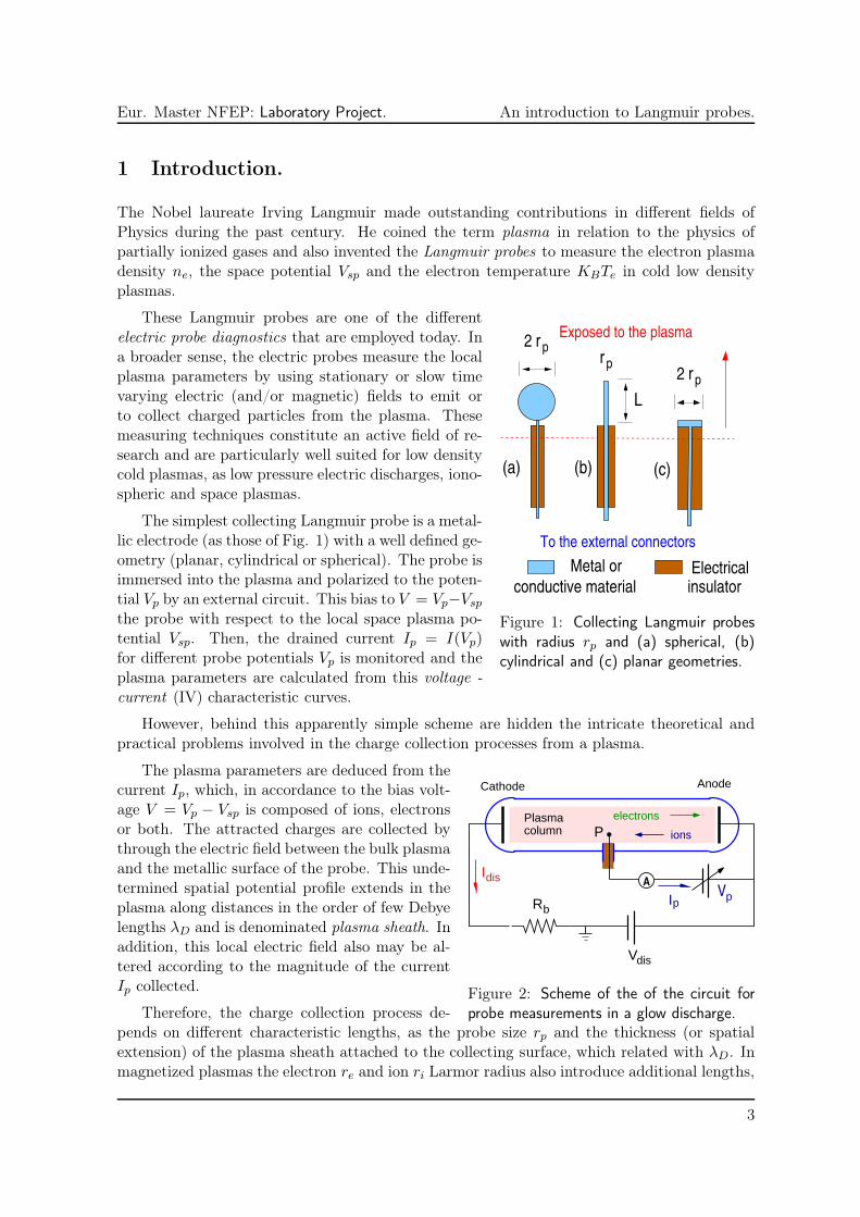
The Nobel laureate Irving Langmuir made outstanding contributions in different fields ofPhysics during the past century. He coined the term plasma in relation to the physics ofpartially ionized gases and also invented the Langmuir probes to measure the electron plasmadensity ne, the space potential Vsp and the electron temperature KBTe in cold low densityplasmas.
These Langmuir probes are one of the different
pr2
pr2
pr
L
(b)(a) (c)
conductive material
Metal or Electricalinsulator
To the external connectors
Exposed to the plasma
Figure 1: Collecting Langmuir probeswith radius rp and (a) spherical, (b)cylindrical and (c) planar geometries.
electric probe diagnostics that are employed today. Ina broader sense, the electric probes measure the localplasma parameters by using stationary or slow timevarying electric (and/or magnetic) fields to emit orto collect charged particles from the plasma. Thesemeasuring techniques constitute an active field of re-search and are particularly well suited for low densitycold plasmas, as low pressure electric discharges, iono-spheric and space plasmas.
The simplest collecting Langmuir probe is a metal-lic electrode (as those of Fig. 1) with a well defined ge-ometry (planar, cylindrical or spherical). The probe isimmersed into the plasma and polarized to the poten-tial Vp by an external circuit. This bias to V = Vp−Vsp
the probe with respect to the local space plasma po-tential Vsp. Then, the drained current Ip = I(Vp)for different probe potentials Vp is monitored and theplasma parameters are calculated from this voltage -
current (IV) characteristic curves.
However, behind this apparently simple scheme are hidden the intricate theoretical andpractical problems involved in the charge collection processes from a plasma.
The plasma parameters are deduced from the
IdisVpIpbR
Vdis
Plasmacolumn P ions
electrons
Cathode Anode
A
Figure 2: Scheme of the of the circuit forprobe measurements in a glow discharge.
current Ip, which, in accordance to the bias volt-age V = Vp − Vsp is composed of ions, electronsor both. The attracted charges are collected bythrough the electric field between the bulk plasmaand the metallic surface of the probe. This unde-termined spatial potential profile extends in theplasma along distances in the order of few Debyelengths λD and is denominated plasma sheath. Inaddition, this local electric field also may be al-tered according to the magnitude of the currentIp collected.
Therefore, the charge collection process de-pends on different characteristic lengths, as the probe size rp and the thickness (or spatialextension) of the plasma sheath attached to the collecting surface, which related with λD. Inmagnetized plasmas the electron re and ion ri Larmor radius also introduce additional lengths,
3

Dept. Física. E.T.S.I. Aeronáuticos. Universidad Politécnica de Madrid
as well as the mean free paths λ for collisions between electrons and/or ions and neutral atomsin collisional and weakly ionized plasmas.
The disparity between these magnitudes, that may differ by orders of magnitude for thedifferent plasmas in nature and/or in measuring systems, leads the theory of Langmuir probesunfortunately incomplete. In fact, no general model is available relating the current voltagecurves I(Vp) with the actual plasma properties under all possible physical conditions.
For unmagnetized Maxwellian plasmas the simplified theory developed by Langmuir andHarold M. Mott-Smith in 1926 allows under ideal conditions to determine the plasma potentialVsp, electron temperature KBTe and density ne ≃ ni. The interpretation of the measurementsoutside the narrow limits of this simplified theory is difficult and many points still remainsobscure.
The idealized situation where the simplified the-
Idis
Vdis
pV
Idc
Vdc
pI
P
Plasma
electrons
ions
Ip
CathodeAnode
A
Figure 3: Scheme of the of the circuitfor probe measurements in a plasmaproduced by thermionic emission ofelectrons.
ory strictly applies is seldom found in the experimentsof interest. However, even in these situations wheredifferent drifting populations of charged particles arepresent or under intense magnetic fields the electricprobes may provide valuable information.
The reader will find these notes as incomplete be-cause they only cover a limited number of topics onLangmuir probe theory. The fundamentals are intro-duced with a detailed deduction of the relevant ex-pressions, however, they do not intend to replace theexcellent monographs and reviews existing in the lit-erature [1, 2, 3, 5]. Our aim is to facilitate to ourstudents an starting point and more involved modelsare left for further readings.
2 Qualitative description of collecting current voltage curves.
The Figs. 2 and 3 represents the two simplest measurement circuits using collecting Lang-muir probes in experiments with cold weakly ionized plasmas. The first case is a glow dis-
charge plasma into a glass tube (or other gas evacuated vessel) with typical pressures between10−2 − 102 mBar. The electric discharge is produced by applying a high DC voltage Vdis
(between 300-600 Volts or more) and the corresponding discharge current Idis is in the rangeof 0.1 − 100 mA. The physical properties of the glow discharge and other electric dischargesare discussed in detail in Ref. [3].
In the scheme of Fig. 3 the wires heated up to red glow by a DC current Ih inside thevacuum chamber to produce the thermoionic emission of electrons. These electrons are lateraccelerated by a discharge voltage Vdis ∼ 20 − 80 Volts, over the first ionization potential ofthe neutral gas, and cause the electron impact ionization of the neutral atoms remaining inthe vacuum chamber. In this case, the discharge current Idis may reach several amps andadditional permanent magnets (not shown in the picture) are frequently disposed around theplasma chamber. This confines the electrons and enhance the local ionization.
4

Eur. Master NFEP: Laboratory Project. An introduction to Langmuir probes.
In both cases, the probe P is immersed at a given point within the plasma biased to theelectric potential Vp with respect to a reference electrode. The anode of the discharge is usedin Figs. 2 and 3. However the cathode or the grounded metallic wall of the plasma chambercould also serve for reference electrode in other situations.
In the following, we will refer to a general probe as
A B
C
D
Vp (Volts)
Probe
current
Vp > VspVp < Vsp
Vp= Vsp
Ies= Ip(Vsp)
Ip(VF) = 0
Vp= VFIis
Figure 4: An idealized IV curve of ob-tained with a collecting Langmuir probein a cold plasma.
those of Fig. 1 with a characteristic length rp. We willspecify if the probe is either, spherical, cylindrical orplanar only when geometry dependent properties arerelevant.
The current-voltage curves (IV) are obtained bymeasuring the drained current Ip by the probe for eachbias potential Vp and Fig. 4 represents an idealizedvoltage current (IV) curve.
In order to give a qualitative interpretation wewill consider an idealized non equilibrium collision-less, Maxwellian and unmagnetized plasma. Thus, thecollisional mean free paths of all particles are largerthan all characteristic lengths (λ ≫ rp, λD) and also
the electron temperature KBTe ≫ KBTi ≃ KBTa is higher than those of ions and neutrals.
The potential Vsp in Fig. 4 corresponds to the electric potential at the point of the plasmawhere the probe is inserted. The collecting probe do not emit particles, and in accordance tothe potential Vp, the drained current Ip = Ii + Ie from the plasma is composed of an ion Iiand electron Ie currents.
For very negative bias voltages Vp ≪ Vsp (at the
r = r p r = r s
Po
ten
tial
Ions
Electrons
pV
(r)
spV
r
bulk plasmaV
Plasma potential
spatial profile
sheath
Met
allic
su
rfac
e
Figure 5: Radial potential profile at-tached to an ion collecting metallic sur-face.
left of point A in Fig.4) the electrons are repelled,while ions are attracted by the probe. The drainedion current from the plasma is limited by the electricshielding of the probe and Ip decreases slowly for verynegative Vp ≪ Vsp. The current Ip ≃ Iis is denomi-nated ion saturation current.
In the opposite limit (voltages at the right of pointC in Fig. 4) where Vp ≫ Vsp the ions are repelled andthe electrons are the attracted charges. In this casethe electrons are responsible for the electric shieldingof the probe and Ip ≃ Ies is called the electron satu-
ration current. The bias potential VF where Ip = 0is the floating potential (point B) where the contribu-tions of the ion and electron currents are equals.
The situation where Vp ≪ Vsp is shown in the scheme of Fig. 5 only an small number ofelectrons have energy enough to jump the potential barrier of Vp. The ions are attracted tothe probe and a layer of negative space charge (negative sheath) develops for r < rs attachedto the metallic surface.
The potential drop from Vsp to Vp and the perturbation caused by the probe electric fieldis concentrated within the space charge layer around the probe, decreases asymptotically in
5

Dept. Física. E.T.S.I. Aeronáuticos. Universidad Politécnica de Madrid
the transition to the unperturbed plasma. The Fig. 6 represents the opposite situation withVp ≫ Vsp where the attracted particles are electrons and again the negative sheath for r < rsconnects the space potential of the unperturbed bulk plasma with Vp.
This effect is quite similar to the plasma polariza-
pV
spV(r)V
Plasma potential
spatial profile
r = r s r = r p
Po
ten
tial
bulk plasma
Ions
Electrons
sheath
r
Met
allic
su
rfac
e
Figure 6: Radial potential profile at-tached to an electron collecting metallicsurface.
tion around a point charge where the spatial fluctua-tions of the plasma potential,
δVsp ∼ (1/r)× exp(−r/λD),
that exponentially decreases with the radial distance.Thus, the thickness of the sheath in Figs. 5 and 6and therefore, the perturbation over the distance rpintroduced in the plasma by the probe is restricted toa few Debye lengths 1.
The vertical doted lines in Figs. 5 and 6 representsthe external surface of the sheath rs around the probe.This boundary is not accurately determined and is thelimit beyond the plasma could be considered again
quasineutral and electric field free. The electrons (or ions) are brought from the bulk plasma tothis boundary mostly by thermal motion. This factor determines the flux of charged particlescrossing the radius rs > rp towards the probe.
Therefore, the attracted charges are collected over the surface defined by rs which couldnot be precisely calculated without solving the Poisson equation to determine V (r). This willbe a key point for attracted particles which enter in the plasma sheath over a surface with anundetermined radius rs > rp.
Figure 7: A cylindrical probe operating in a glow discharge plasma (left) and a closer view for largeposive bias (right). In weakly ionized plasmas, this glow is produced for Vp ≫ Vsp by the inelasticcollisions between neutral atoms and attracted electrons in the sheath.
The plasma sheath formed by attracted electrons can be visualized in a weakly ionizedplasma by the bright glow surrounding the cylindrical probe in Fig. 7. Because of the largeneutral gas atom density, the inelastic collisions of neutrals with the accelerated electrons inthe sheath produce the emission of light. The large electron currents heat the probe and thisfact is also used for probe surface cleaning.
1The structure of the ion sheath is discussed in detail in Sec. 8.2 pp. 290-295 of Ref. [4].
6

Eur. Master NFEP: Laboratory Project. An introduction to Langmuir probes.
On the contrary, the repelled charges with thermal energy enough to overcome the potentialbarrier and to reach the probe are collected over its surface. The drained current Ip of attractedparticles (for either Vp ≫ Vsp and Vp ≪ Vsp) becomes therefore weakly dependent of Vp asshown in Fig. 4. This saturation process by attracted particles is in the origin of the currentsIis and Ies which are respectively the ion and electron saturation currents.
The electrons are repelled for probe bias
Collectedelectrons
en (E)
(eVsp )
E=0
)spp VVe(> > 0
= eVp> 0
Electron energy E
pE
E p
Ele
ctro
n d
ensi
ty
Figure 8: Electron collection process in the re-tarding field region (curve BC) of Fig. 4.
Vp − Vsp < 0 below the local plasma poten-tial. The Fig. 8 represents the fraction ofcollected electron with energy enough to reachthe probe because of the finite electron tem-perature KBTe of the Maxwellian energy dis-tribution.
The number of electrons with energy,
E = −e(Vp − Vsp) ≥ 0
that reach the probe increases as the biasVp − Vsp with respect to the bulk plasma de-creases. This fact explains the abrupt grow-
ing of Ip in Fig. 4 between B and C which is strongly dependent of Vp, contrary to the currentsaturation processes (over point C and below B). This part of the IV curve is frequentlydenominated electron retarding field because the probe bias Vp repels a fraction of electronsfrom reaching the probe.
Finally, when Vp = Vsp no sheath develops around the probe and the charges reach itssurface because of their thermal motion. Thus, the probe collects the thermal flux of bothelectrons Γe,Th and ions Γi,Th. In consequence, the probe biased at the space plasma potentialdrains an electric current from the plasma even in the absence of potential difference betweenthe conductor and the surrounding plasma.
The thermal flux of electrons (α = e) and (α = e) ions is given by,
Γα,Th =1
4nα
(
8KBTe
πmα
)1/2
and their density currents are, Iα.Th = qα Γα,Th. Because, mi ≫ me 1 and KBTe ≫ KBTi onpractical grounds,
Ip = Ie,Th + Ii,Th = Ie,Th
(
1 +Ie,Th
Ii,Th
)
≃ Ie,Th
and therefore, the current Ip(Vp) in Fig. 4 is equal to the electron thermal and saturationcurrents Ip(Vp) ≃ Iet = Ies ≫ Iis.
The next step is to calculate the plasma parameters from the IV curve fitting obtainedin the experiments. This requires of physical models relating the drained current Ip with theenergy distribution functions of charged particles. Unfortunately, because of the wide rangeof plasma densities, temperatures and characteristic lengths the results are quite unrealistic ifthe wrong model is employed.
7
Dept. Física. E.T.S.I. Aeronáuticos. Universidad Politécnica de Madrid
3 The simplified theory for collisionless unmagnetized plasmas.
The simplest model relating the plasma properties with current voltage curves was formulatedby Langmuir and Mott-Smith and is valid for unmagnetized collisionless Maxwellian plasmas.The following formulation of the theory essentially comes from Ref. [5] and these calculationsrely on some assumptions that apply to most of nonequilibrium laboratory plasmas.
1. The bulk plasma volume is considered as infinite, stationary, homogeneousand quasineutral ne ≃ ni.
2. Electron and ions have Maxwellian distributions of velocities and the kinetictemperature of the species are KBTe ≫ KBTi ≃ KBTa, where α = e, i, arepresents respectively electrons, ions and neutral atoms.
3. The collisional mean free paths of electrons λe and ions λi are larger than rpand λD.
4. The charged particles that reach the surface of the probe do not chemicallyreact with the probe material, are always collected and contribute to theprobe current I(Vp).
5. The perturbation introduced by the probe in the plasma is confined to a spacecharge sheath with a well defined boundary. Outside this sheath the spacepotential is assumed uniform in the bulk plasma.
6. The sheath thickness d ≪ rp is small compared with the characteristic probedimension and therefore edge effects may be neglected.
7. The potential around the probe preserves the symmetry (spherical, cylindricalor planar) and V (r) is a monotonically decreasing (or increasing) functionbetween the sheath edge and the probe surface.
First of all, we will consider the motion of a charge qα (α = e, i) of mass mα, located at theradial distance r with initial speed v. This particle moves close to a cylindrical or sphericalprobe and we will use in the following e = |e| > 0, then qe = −e for electrons and qi = +e forions.
The bulk plasma is considered as stationary and uniform in space (see previous points 1,3 and 5) and the plasma potential takes an uniform value Vsp. For the a radial distance r theelectric potential with respect to this undisturbed plasma is φ(r) = V (r)− Vsp and the probepotential is φp = V (rp)− Vsp.
It is of worth to recall that the plasma potential profile around the probe φ(r) = V (r)− Vsp
remains undetermined. The only requisite (see previous points 5, 6 and 7) for the sheathpotential φ(r) is to be a monotonic function decreasing or increasing fast enough close to theprobe surface as in Figs. 5 and 6.
Two different situations arise, the charge qα could be repelled by the retarding electric field
around the probe when qα φ(r) > 0. For electrons corresponds to the BC part of the IV curveof Fig. 4). On the contrary, the particle may be also attracted by the accelerating field whenqα φ(r) < 0 (in Fig. 4 the parts AB for ions and CD for electrons).
8

Eur. Master NFEP: Laboratory Project. An introduction to Langmuir probes.
3.1 Spherical probe
In the case of the spherical probe, the motion of a single charge is restricted to a planedefined by its velocity v and the plane of symmetry of the sphere. As in Fig. 9, the speedv = v⊥ + v‖ has two components v‖ parallel and perpendicular v⊥ to the radial directioner, normal to the probe surface. The charge that reaches the probe surface rp with speedv
′
= v′‖ + v′
⊥ comes from the radial distance r ≥ rp with the initial velocity v.
In the absence of collisions the energy of this
pr
er
VV||
Vprobe
Figure 9: The scheme of the spherical probeand the components of the charge velocity.
particle is conserved,
mα
2(v2‖ + v2⊥) + qαVsp =
mα
2(v′
2‖ + v′
2⊥) + qαVp
and also for the component of the angular mo-mentum perpendicular to the plane of Figs. 9and 10,
r v⊥ = rp v′⊥ and, v′⊥ =
r
rpv⊥
Setting φp = Vp − Vsp we have,
V
VV||
pr
ereθds
r
ϕ
ϕ
Figure 10: The velocityv = v‖ + v⊥ of the chargecrossing the surface element dSplaced at the radial distance r.
v′2= v2‖ + v2⊥
(
1− r2
r2p
)
− 2 qαmα
φp ≥ 0
In order to be collected v′ ≥ 0 and this relates the mag-nitude of the angular v⊥ and radial v‖ components of thevelocity of collected charges,
v2⊥ ≤v2‖ − 2qαφp/mα
(r/rp)2 − 1
As shown in Fig. 10 the components of the speed are,v⊥ = v sin ϕ and v‖ = v cos ϕ,
v2 sin2 ϕ ≤ v2 cos2 ϕ− 2qαφp/mα
(r/rp)2 − 1
From this expression we obtain the maximum allowed angleϕm of the particle velocity v with the radial direction erof Fig. 10 for the distance r,
sin2 ϕm ≤r2pr2
(
1− 2 qαφp
mαv2
)
=r2pr2
(
1− qαφp
E
)
(1)
This latter depends on the radial distance r to the probe and the ratio between the electrostaticenergy (qαφp) and the initial kinetic energy E of the incoming charge.
The key point of collecting Langmuir probe theory is to relate the energy spectrum of theattracted or repelled particles with current drained by the probe. Therefore, in order to relate
9

Dept. Física. E.T.S.I. Aeronáuticos. Universidad Politécnica de Madrid
I(rp) with the plasma properties, instead of a monoenergetic charged particle, we consider avelocity distribution function fα(v). Then, for each charged specie in the plasma,
dnα = nαo fα(v) dv
represents the number of particles by volume unit of the specie α with velocities between v
and v + dv. The above distribution function fα(v) is normalized to,
∫ +∞
−∞fα(v) d
3v = 1
and nαo represents the density of particles of the specie α in the undisturbed bulk plasma.
3.1.1 Repelled particles
For repelled particles qαφp > 0 and positive values of Eq. (1) require the kinetic energy ofcharges E ≥ qα φp, also r ≥ rp for sin2 ϕ ≤ 1. Therefore, the probe collects over its surfaceonly the repelled particles with energy enough to overcome the potential barrier.
Because of the symmetry, the current density dj(r) over dS in Figs. 10 and 11 of chargesattracted or repelled by the spherical is parallel fo er and,
(dj)‖ = dj = qα v‖ dnα
The details of the integration over the surface dS are in Fig. 11, and using dv = v2 sinϕdθ dϕdvwe have,
dj = (qαnαo) (v cosϕ) v2 sinϕfα(v) dv dθ dϕ (2)
Now, we make an important assumption: the velocity distribution function is isotropic, onlydepends of the energy of particles, fα(v) = fα(|v|), we obtain,
j(r) = (qαnαo)
∫ ∞
vm
v3fα(v) dv
∫ 2π
0dθ
∫ ϕm
0sinϕ cosϕdϕ
For repelled charges (qαφp > 0) a minimum initial energy (or speed) mv2m/2 ≥ qα φp isnecessary to overcome the potential barrier around the probe. Therefore,
j(r) = (qαnαo)π
∫ ∞
vm
v3fα(v) sin2 ϕm dv
and sinϕm is eliminated by using Eq. (1),
j(r) = (qαnαo)π
(
r2pr2
)
∫ ∞
√2qαφp/mα
v3fα(v)
(
1− 2qαφp
mαv2
)
dv (3)
This last expression only depends on the particle velocity v and decreases with the radialdistance. In the absence of ionizations and charge losses for r ≥ rp for particles with v ≥ vmthe probe current is, I(r) = I(rp) and I(rp) = (4πr2) j(r) and finally we have,
10

Eur. Master NFEP: Laboratory Project. An introduction to Langmuir probes.
I(rp) = (qαnαo)π Asph
∫ ∞
√2 qαφp/mα
v3fα(v)
(
1− 2 qαφp
mαv2
)
dv (4)
where Asph = 4πr2p is the area of the spherical probe.
The Eqs. (3) and (4) are usually are made dimensionless using the thermal speed,
c =
√
2KBTα
mα
where KBTα is the kinetic temperature of the specie α. The
er
mϕ−
V||
mϕ+
ds
θ
Figure 11: The angles con-sidered over a surface elementdS in Eq.(2).
scaled velocity is u = v/c and um =√
φp with φp = qφp/KBTα.This dimensionless probe potential compares the electrostatic(eφp) and thermal (KBTα) energies of particles. Thus,
j(r) = (qαnαo)π c4
(
r2pr2
)
∫ ∞
√φp
u3fα(u)
(
1− φp
u2
)
du (5)
The above integrals could be evaluated for the particularcase of the Maxwell Boltzmann velocity distribution function,
f(u) =1
π3/2 c3e−u2
(6)
Using,∫ ∞
um
u3 e−u2
(
1− u2mu2
)
du =e−u2
m
2
we obtain a simple expression for the current of repelled particles,
j(r) =qα nαo
4Vth exp
(
qα (Vsp − Vp)
KBTα
)
(7)
where Vth = (8KBTα/πmα)1/2 and also,
I(rp) =qα nαoAsph
4Vth exp
(
qα (Vsp − Vp)
KBTα
)
(8)
This exponential growth of the current is in accordance with the expected response for electronsof the ideal probe along the segment BC in Fig. 4. When the probe is biased at the localplasma potential (Vp = Vsp or φp = 0) the current collected is the random flux of charges toits surface,
I(Vp) =qα nαo Asph
4Vth (9)
11

Dept. Física. E.T.S.I. Aeronáuticos. Universidad Politécnica de Madrid
3.1.2 Attracted particles
For attracted charges setting qαφp = −|qαφp| < 0 in Eq. (1),
sin2 ϕm ≤r2pr2
(
1 +2 |qαφp|mαv2
)
=r2pr2
(
1 +|qαφp|E
)
(10)
Thus, the behavior of the particle orbits depend on whether the initial particle velocities aresmaller or larger that a certain velocity vs defined by the radial distance,
rs = rp
√
1 +|qαφp|E
which is rs > rp for E > 0. For a fixed (and at this point undetermined) value of rs the speedvs from Eq. (10) is,
v2s =2 |qαφp|
mα(r2s/r2p − 1)
that defines the energy Es = mαv2s/2 leading sinϕm = 1 in Eq. (10).
The radial distance rs, that could be identified with the sheath threshold of Figs. 5 and6, and cannot be precisely determined at this point without solving the Poisson equation todetermine the plasma potential profile φ(r) around the probe.
Therefore, for r = rs the particles with E ≤ Es are collected because the Eq. (10) is alwayssatisfied. The radial distance rs plays the role of threshold radius for the particle orbits andthe motion of the charges to the probe is said sheath limited. For v > vs and r = rs only thoseparticles with sin2 ϕ ≤ 1 are collected while others orbit or their trajectories bend around theprobe. The motion of the charges is said to be orbit limited.
For accelerated particles the current density dj‖(r) going into dS in Figs. 10 and 11 iscomposed of two terms, dj(rs) = djsl(rs) + djol(rs) according to the velocity of the incomingcharges with,
jsl(rs) = (qαnαo)
∫ vs
0v3fα(v) dv
∫ 2π
0dθ
∫ π
0sinϕ cosϕdϕ
also,
jol(rs) = (qαnαo)
∫ ∞
vs
v3fα(v) dv
∫ 2π
0dθ
∫ ϕm
0sinϕ cosϕdϕ
After the integration and using Eq. (10) for sin2ϕm we have,
j(rs) = (qαnαo)π
[
∫ vs
0v3fα(v) dv +
(
r2pr2s
)
∫ ∞
vs
v3fα(v)
(
1 +2 |qαφp|mαv2
)
dv
]
(11)
As before, the probe current is I(rp) = 4πr2s j(rs) and then,
I(rp) = (qαnαo)π
[
(4πr2s)
∫ vs
0v3fα(v) dv + (4πr2p)
∫ ∞
vs
v3fα(v)
(
1 +2 |qαφp|mαv2
)
dv
]
(12)
12

Eur. Master NFEP: Laboratory Project. An introduction to Langmuir probes.
Now, in order to calculate the final result for particular case of the Maxwell Boltzmanndistribution (Eq. 6) we introduce the equivalent dimensionless expression to Eq. (11),
j(rs) = (qαnαo)π c41
π3/2 c3
[
∫ us
0u3fα(u) du +
(
r2pr2s
)
∫ ∞
us
u3fα(u)
(
1 +|φp|u2
)
du
]
where us = vs/c. Then,
j(rs) = (qαnαo)c√π
[
∫ us
0u3 e−u2
du +
(
r2pr2s
)
∫ ∞
us
u3e−u2
(
1 +|φp|u2
)
du
]
and using the integrals,
∫ us
0u3 e−u2
du =1
2
[
1− e−u2s (1 + u2s)
]
∫ ∞
us
u3 e−u2
(
1 +|φp|u2
)
du =e−u2
s
2
[
1 + u2s + |φp|]
this leads to,
j(rs) = (qαnαo)c
2√π
[
1 + e−u2s
(
(r2pr2s
− 1) + u2s (r2pr2s
− 1) +r2pr2s
|φp|)]
The final expression is,
j(rs) = (qαnαo)c
2√π
[
1 + (r2pr2s
− 1)e−u2s
]
(13)
and the collected current coincides with the Eq. (29) of Ref. [5],
I(rp) =Asph
4(qαnαo)Vth
r2sr2p
[
1− (1−r2pr2s
) exp
(
−r2p
r2s − r2p
|qαφp|KBTα
)]
(14)
3.2 Cylindrical probe
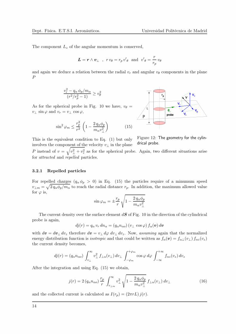
The scheme with the motion of particles in the cylindrical geometry is represented in Fig. 12where we assume the probe with a length L ≫ rp much larger than its radius. As for thespherical probe, the velocity at rp is v′ and v at the radial distance r > rp. The speed vzalong the Z axis is constant and the Fig. 10 also applies for the component v⊥ = vr + vθ inthe plane P perpendicular to the probe axis with v‖ ≡ v (compare with Fig.12). Therefore,
mα
2(v2r + v2θ + v2z)− qαφp =
mα
2(v′
2r + v′
2θ + v2z)
13
Dept. Física. E.T.S.I. Aeronáuticos. Universidad Politécnica de Madrid
The component Lz of the angular momentum is conserved,
L = r ∧ v⊥ , r vθ = rp v′θ and v′θ =
r
rpvθ
and again we deduce a relation between the radial vr and angular vθ components in the planeP
er
Vz
Vr
VθV
prV
probe
L
P
Figure 12: The geometry for the cylin-drical probe.
v2r − qα φp/mα
(r2/r2p − 1)≥ v2θ
As for the spherical probe in Fig. 10 we have, vθ =v⊥ sinϕ and vr = v⊥ cosϕ,
sin2 ϕm ≤r2pr2
(
1− 2 qαφp
mαv2⊥
)
(15)
This is the equivalent condition to Eq. (1) but onlyinvolves the component of the velocity v⊥ in the plane
P instead of v =√
v2⊥ + v2z as for the spherical probe. Again, two different situations arise
for attracted and repelled particles.
3.2.1 Repelled particles
For repelled charges (qα φp > 0) in Eq. (15) the particles require of a minumum speedv⊥m =
√
2 qαφp/mα to reach the radial distance rp. In addition, the maximum allowed valuefor ϕ is,
sinϕm = ±rpr
√
1− 2 qαφp
mαv2⊥
The current density over the surface element dS of Fig. 10 in the direction of the cylindricalprobe is again,
dj(r) = qα vr dnα = (qαnαo) (v⊥ cosϕ) fα(v) dv
with dv = dv⊥ dvz therefore dv = v⊥ dϕ dv⊥ dvz. Now, assuming again that the normalizedenergy distribution function is isotropic and that could be written as fα(v) = fα⊥(v⊥) fαz(vz)the current density becomes,
dj(r) = (qαnαo)
∫ ∞
v⊥
v2⊥ f⊥α(v⊥) dv⊥
∫ +ϕm
−ϕm
cosϕ dϕ
∫ +∞
−∞fαz(vz) dvz
After the integration and using Eq. (15) we obtain,
j(r) = 2 (qαnαo)rpr
∫ ∞
v⊥m
v2⊥
√
1− 2 qαφp
mαv2⊥f⊥α(v⊥) dv⊥ (16)
and the collected current is calculated as I(rp) = (2πrL) j(r).
14

Eur. Master NFEP: Laboratory Project. An introduction to Langmuir probes.
I(rp) = 2Acyl (qαnαo)
∫ ∞
v⊥m
v2⊥
√
1− 2 qαφp
mαv2⊥
f⊥α(v⊥) dv⊥ (17)
where Acyl = 2πrpL is the surface of the probe.
For the particular case of the Maxwell Boltzmann
V
erVr
Vz
pr
ϕL
r
dS
probeP
Figure 13: The velocity v = v⊥ + vzof a charge over the surface element dsplaced at the radial distance r.
distribution (Eq. 6) using the dimensionless velocityu = v⊥/c as before,
j(r) = 2 (qαnαo)rpr
∫ ∞
um
u2 e−u2
√
1− φp
u2du
and in this case,
∫ ∞
um
u2 e−u2
√
1− φp
u2du =
√π
4e−u2
m
The final values for the current density at the radialdistance r is,
j(r) =rpr
(qαnαo)Vth
4exp
(
φp
)
=rpr
(qαnαo)Vth
4exp
(
qαφp
KBTα
)
(18)
and the current collected by the probe is,
I(rp) =(qαnαo)Vth Acyl
4exp
(
qα(Vp − Vsp)
KBTα
)
(19)
Thus, for a Maxwellian plasma the current of repelled particle for spherical and cylindricalprobes only differ by a geometrical factor, Asph or Acyl. Again, when the probe is biased tothe plasma potential φp = 0 and collects the thermal flow of particles,
I(Vp) =(qαnαo)Acyl
4Vth
3.2.2 Attracted particles
For attracted charges qα φp < 0 and the Eq. (15) becomes,
sin2 ϕ =r2pr2
(
1 +2 |qαφp|mαv2⊥
)
(20)
which defines the radial distance rs > rp and the critical speed v⊥s. According to the velocityof the attracted charges, as for the spherical probe, the radial component of the current densityat the distance rs is the sum dj(rs) = djsl(rs)+djol(rs) of the sheath limited and orbit limitedparts . In this case using vr = v⊥ cosϕ and,
(dj)r = dj(rc) = qα vr dnα = (qαnαo) (v⊥ cosϕ)fα(v) dv
15

Dept. Física. E.T.S.I. Aeronáuticos. Universidad Politécnica de Madrid
Assuming an anisotropic velocity distribution function, with the details of the integration asindicated in Fig. 13,
jsl(rs) = (qαnαo)
∫ v⊥s
0v2⊥fα⊥(v⊥) dv⊥
∫ π
−πcosϕdϕ
∫ +∞
−∞fαz(vz) dvz (21)
and,
jol(rs) = (qαnαo)
∫ ∞
v⊥s
v2⊥fα⊥(v⊥) dv⊥
∫ ϕm
−ϕm
cosϕdϕ
∫ +∞
−∞fαz(vz) dvz
Using the Eq. (20) the integration leads to,
j(rs) = 2 (qαnαo)
∫ v⊥s
0v2⊥fα⊥(v⊥) dv⊥ +(qαnαo)
rprs
∫ ∞
v⊥s
v2⊥
√
1 +2 |qαφp|mαv
2⊥
fα⊥(v⊥) dv⊥ (22)
The corresponding current is I(rp) = (2π rs L) j(rs). Because of the cylindrical symmetry,this last equation involves the two dimensional velocity distribution function fα⊥(v⊥). Thedimensionless Eq. (22) with u = v⊥/c is,
j(rs) = (qαnαo)2 c
π
2
∫ us
0u2fα⊥(u) du +
rprs
∫ ∞
us
u2 fα⊥(u)
√
1 +|φp|u2
du
and for the particular case of the two dimensional Maxwell Boltzmann distribution,
f2d(u) =2
π ce−u2
we obtain,
j(rs) = (qαnαo)2c
π
∫ us
0u2e−u2
du +rprs
∫ ∞
us
u2 e−u2
√
1 +|φp|u2
du
The values of these integrals are,
∫ us
0u2e−u2
du =1
4
[
−2 us e−u2
s +√π Erf(us)
]
∫ ∞
us
u2 e−u2
√
1 +|φp|u2
du =e−u2
2
√
u2s + |φp|+√π
4e|φp| Erfc(
√
u2s + |φp| )
where Erf(x) and Erfc(x) are the error and the complementary error functions. After somemanipulations we obtain,
j(rs) =1
4(qαnαo)Vth
[
Erf(us) +rpre|φp| Erfc(
√
u2s + |φp| )]
(23)
and also for the current I(rp) = (2φ rs L) j(rs),
I(rp) =Acyl
4(qαnαo)Vth
[
rsrp
Erf(us) + e|φp| Erfc(
√
u2s + |φp| )]
(24)
16

Eur. Master NFEP: Laboratory Project. An introduction to Langmuir probes.
3.3 Approximations
For the particular case of the Maxwell Boltzmann velocity distribution the the results (Eqs. (7)and (18)) are equivalent and independent of the geometry of the probe for repelled particles.On the contrary, for attracted charges are different the Eqs. (13) for the spherical probe andEqs.(23) for the cylindrical geometry 2.
In addition, the above results for accelerating fields contains the radial distance rs thatcould be identified with the sheath edge. This distance would mark the threshold betweenthe bulk unperturbed plasma and the plasma sheath, as indicated in Figs. 5 and 6. In fact,such radius is undetermined as well as the plasma potential drop φ(r) around the probe. Thiscalculation is complex and involves Poisson equation for the electric field around the probe,which is also influenced by the local spatial charge distribution in the sheath.
Therefore, some approximations are required to eliminate rs from the above expressionsfor attracted particles. They compare the probe radius rp with the radial distance rs of thesheath limit. The thin sheath approximation corresponds to rs − rp ≫ rp while in the thick
sheath limit rs ≫ rp.
3.3.1 The thin sheath limit
In this case the normalized speed,
u2c = |φp|r2p
r2s − r2p
is large in the limit rs − rp ≫ rp. Thus, writing Ies = Asph (qαnαoVth)/4 the Eq. 14 reads,
I(rp) = Iesr2sr2p
[
1− (1−r2pr2s
)e−u2c
]
and using exp(−u2c) ≃ 1 we obtain,
I(rp) ≃ Iesr2sr2p
(
1− 1 +r2pr2s
)
= Ies
Therefore, the current of attracted particles for an spherical probe in the thin sheath limit isconstant for bias voltages Vp ≫ Vsp.
For the cylindrical probe, with Ies = Acyl (qαnαoVth)/4 the Eq. 24 reads,
I(rp) = Ies
[
rsrp
Erf(uc) + e|φp| Erfc(
√
u2c + |φp| )]
= Ies F ( uc, |φp|)
and in the limit rs − rp ≫ rp we may use of,
Erfc(x) = 1− Erf(x) ≃ 1√π
e−x2
x
2These expressions corresponds to Eqs. (29) and (30) in Ref. [5] and (43-49) in Ref. [7].
17

Dept. Física. E.T.S.I. Aeronáuticos. Universidad Politécnica de Madrid
for large values of x. Thus, the function F ( uc, |φp|) can be approximated by,
F ( uc, |φp|) ≃rsrp
(1− 1√π
e−u2
u) +
e|φp|
√π
e−u2
e−|φp|
√
u2c + |φp|
And we have,
u2c + |φp| = |φp|r2p
r2s − r2p+ |φp| =
r2sr2p
u2c
After some simple manipulations we obtain,
F ( uc, |φp|) ≃rsrp
(
1− 1√π
r2pr2s − r2p
r2pe−u2
u
)
≃ rsrp
∼ 1
Therefore, in the thin sheath limit the current of attracted charges collected by both, the cylin-drical and spherical probes I = Ies is equal to the electron saturation current and independentof the probe bias for Vp ≫ VSp.
3.3.2 The thick sheath limit
For the spherical probe when rs/rp ≫ 1 we approximate,
exp (−u2c) = exp
[
−|φp|1
r2s/r2p − 1
]
≃ exp
(
−|φp|r2pr2s
)
∼ 1− |φp|r2pr2s
and in Eq. (14) we have,
I(rp) ≃Asph
4(qα nαo)Vth
[
r2sr2p
− r2sr2p
(
1−r2pr2s
) (
1−r2pr2s
|φp|)]
Writing Ies = (Asph qα nαo Vth)/4 we obtain,
I(rp) ≃ Ies
(
1 + |φp| −r2pr2s
|φp|)
Finally, neglecting the small term,
I(rp) ≃ Ies (1 +|qαφp|KBTα
) (25)
In the thick sheath limit the collected current of attracted particles for the spherical probegrows linearly with the bias potential Vp ≫ Vsp.
In the case of the cylindrical geometry,
F ( uc, |φp|) =rsrp
Erf(uc) + e|φp| Erfc (rsrp
uc)
18

Eur. Master NFEP: Laboratory Project. An introduction to Langmuir probes.
and because rs ≫ rp for low values of uc we make use of Erf(x) ≃ (2x)/√π,
F ( uc, |φp|) ≃rsrp
2√πuc + e|φp| Erfc (
rsrp
uc)
After some simple manipulations we obtain,
F ( uc, |φp|) ≃2√π
√
φp + e|φp| Erfc (
√
φp)
On the contrary, the argument of Erfc (√
φp) ≃ Erfc (rsuc/rp) is large and we could make useof the previous approximation. Then,
F ( uc, |φp|) ≃2√π(
√
φp +1
2
1√
φp
) ∼ 2√π(1 + |φp|)1/2
The final expression for the cylindrical probe is,
I(rp) = Ies2√π(1 +
|qαφp|KBTα
)1/2 (26)
For Maxwellian plasmas where the thick sheath approximation is valid, the Eqs. (25) and(26) suggest that KBTα could be determined by plotting Ip (or I2p) aganist φp = Vp − Vsp.The density unperturbed density nαo also may be determined from the value of Ise.
-5 -4 -3 -2 -1 0 1 2 3 4 5Normalized bias potential (φp = eVp/KBTe)
0
1
2
Nor
mal
ized
cur
rent
( I/
I se )
CylinderSphere
Thick sheath approximation
( φsp = 2 )
VF
(a)
-2 -1 0 1 2 3 4 5Normalized bias potential ( φp = eVp/KBTe)
0,01
0,1
1
Nor
mal
ized
cur
rent
( I/
I se )
CylinderSphereLeast squares fit
Thick sheath approximation
(φsp = 2)
exp (-(φsp-φp) )Fit to
(b)
Figure 14: Comparison of the thick sheath approximation for spherical and cylindrical probes in(a) linear and in (b) logarithmic axis for an Argon plasma. The electron temperature is KBTe = 3eV and the ion temperature KBTi = 0.013 eV (equivalent to the room temperature of 300 K ).The plasma potential is Vsp = 6 V, (φsp = 2 V with φsp = e Vsp/KBTe).
19

Dept. Física. E.T.S.I. Aeronáuticos. Universidad Politécnica de Madrid
The results of the thick sheath approximation for a typical plasma are represented in Fig.14 and have a similar look to the idealized current voltage curve of Fig. 4. The curves alsocompare the Eq. (25) for spherical and Eq. (26) for cylindrical geometries. In the electronsaturation region (CD in Fig. 4 where Vp > Vsp) the current is geometry dependent whilethis is not the case for repelled electrons (AC in Fig. 4 where V < Vsp). This fact is causedby the low temperatures and large mass of ions that increase for Vp < Vsp the ion saturationcurrent less than Ise for V > Vsp.
We conclude that the equations (25) and (26) lead to an important result. When the thick
sheath approximation is valid in Maxwellian plasmas, the repelled particle temperature KBTα
could be determined by plotting Ip (or I2p) against φp = Vp − Vsp. Once KBTα is obtained,the plasma density nαo may be determined from the value of Ies = A (qα nα)VTh/4.
However, as we shall see the validity of this approximation is limited when compared withactual experimental data (see Fig. 16 and the discussion in Sec. 4.1). In this thick sheath
approximation the electric field around the probe remains undetermined because the Poissonequation has been ignored. Thus, more involved models are required to account for the orbitalmotion of attracted charges.
3.4 The energy distribution function of repelled particles
Finally, without making assumptions regarding the energy distribution function g(E) andimportant result is deduced from Eqs. (4) and (17) for both geometries. [2, 9]. Deriving withrespect of the lower limit of the integrals,
I(α) =
∫ b
af(x, α) dx
we have,
dI
dα= f(b, α)
db
dα− f(a, α)
da
dα+
∫ b
a
∂f(x, α)
∂xdx
From Eq. (4) for the spherical probe we obtain,
I(rp) =Asph qα
4
∫ ∞
qαφp
(1 +qαφp
E) g(E)
√
2E
mαdE
Therefore,
d2I
dφ2p
= 0− 0 +
∫ ∞
qαφp
q2απr2p
E(1 +
qαφp
E) g(E)
√
2E
mαdE
and,
d2I
dφ2p
= −(q2απr2p) g(E)
√
2qαmαφp
We conclude distribution energy for repelled particles can be calculated from the second dif-ferential of the current with respect to the bias voltage,
20

Eur. Master NFEP: Laboratory Project. An introduction to Langmuir probes.
g(E) = − 1
(q2απr2p)
√
mαφp
2qα
(
d2I
dφ2p
)
This result is valid for any geometry as far as the velocity distribution is isotropic. Then,even for non Maxwellian plasmas, the distribution function of repelled particles g(E) can beobtained from the experimental data. While this result is valid for any kind of repelled charge,in of particular interest for the electrons.
However High noise of the initial curve makes it very difficult to obtain the second differ-ential of the current with respect to the bias voltage.
4 Interpretation of Langmuir probe data for repelling electrons
The above simplified theory considers an isotropic equilibrium plasma where none privilegeddirection for the particle speed exists. This is not the case for a large number of situationsof physical interest where the probe and/or the plasma are in relative motion. However, theabove theory only applies as far as the drift velocity of the plasma is low compared with thethermal speed of charges. This is also a common situations in low pressure discharge plasmas.
However, even when the energy distribution function is non Maxwellian, some importantinformation could be obtained using collecting Langmuir probes. As we have seen, the repelledcharges are collected over the surface S of the probe and Eq. (5) for the spherical and Eq.(16) for cylindrical geometry are valid for any isotropic velocity distribution function fα(u).
In general, the repelled charge current of the specie α may be directly connected with fα(u),this is of relevance for the repelled electrons. The electrons are mainly concerned because ofthe lower ion temperature, that leads the repelled ion currents to be one or two orders ofmagnitude much smaller than the electron currents in most experiments [2].
4.1 The analysis of experimental results
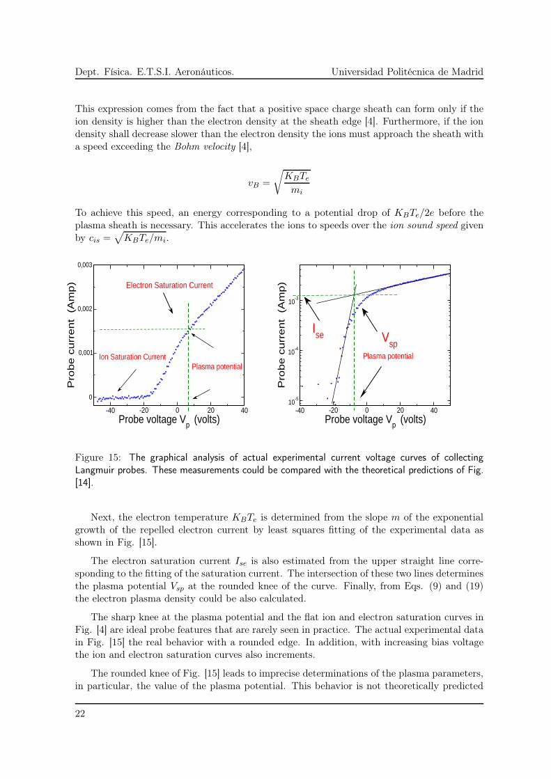
The classical analysis of the IV curves of collecting Langmuir curves is simple and based inthe fact that Eqs. (8) and (19) are geometry independent. This calculation has been subjectof a large number of refinements but its basic scheme has not been changed since the earlywork of Irvin Langmuir.
The first step is to subtract to all experimental data the value of the ion saturation current.This moves upwards the curve leading all currents positive. However, this value is frequentlyso small that this correction becomes negligible as for the experimental data shown in Fig.[15]. For low temperature plasmas where Ti ≪ Te the ion saturation current is approximatedclose to the floating potential by the Bohm relation [4],
Iis = IBohm = 0.6ni e S
√
KBTe
mi
The factor 0.6 = e−1/2 comes from the approximation of the plasma potential Vsp ≃KBTe/2 at the end of the presheath [4].
21
Dept. Física. E.T.S.I. Aeronáuticos. Universidad Politécnica de Madrid
This expression comes from the fact that a positive space charge sheath can form only if theion density is higher than the electron density at the sheath edge [4]. Furthermore, if the iondensity shall decrease slower than the electron density the ions must approach the sheath witha speed exceeding the Bohm velocity [4],
vB =
√
KBTe
mi
To achieve this speed, an energy corresponding to a potential drop of KBTe/2e before theplasma sheath is necessary. This accelerates the ions to speeds over the ion sound speed givenby cis =
√
KBTe/mi.
-40 -20 0 20 40Probe voltage Vp (volts)
0
0,001
0,002
0,003
Pro
be
cu
rre
nt
(A
mp
)
Ion Saturation Current
Electron Saturation Current
Plasma potential
-40 -20 0 20 40Probe voltage Vp (volts)
10-5
10-4
10-3
Pro
be
cu
rre
nt
(A
mp
)
Ise
Plasma potential
Vsp
Figure 15: The graphical analysis of actual experimental current voltage curves of collectingLangmuir probes. These measurements could be compared with the theoretical predictions of Fig.[14].
Next, the electron temperature KBTe is determined from the slope m of the exponentialgrowth of the repelled electron current by least squares fitting of the experimental data asshown in Fig. [15].
The electron saturation current Ise is also estimated from the upper straight line corre-sponding to the fitting of the saturation current. The intersection of these two lines determinesthe plasma potential Vsp at the rounded knee of the curve. Finally, from Eqs. (9) and (19)the electron plasma density could be also calculated.
The sharp knee at the plasma potential and the flat ion and electron saturation curves inFig. [4] are ideal probe features that are rarely seen in practice. The actual experimental datain Fig. [15] the real behavior with a rounded edge. In addition, with increasing bias voltagethe ion and electron saturation curves also increments.
The rounded knee of Fig. [15] leads to imprecise determinations of the plasma parameters,in particular, the value of the plasma potential. This behavior is not theoretically predicted
22

Eur. Master NFEP: Laboratory Project. An introduction to Langmuir probes.
in Fig. [14] for the thick sheath approximation where the effect of the local electric field isneglected. This suggests that the sheath formed around the probe would be responsible forthis behavior.
Because of the electric imperfect probe shielding of electrons close to Vsp, the expansionof the plasma sheath is the more accepted explanation for this round off observed in Fig. 15[1, 2].
However, this point is unclear, the plasma sheaths around the probe are small in weaklyionized plasmas with densities in the order of ∼ 108 cm−3 and Te ≈ 2 eV. The typical sheaththickness, in the order of the Debye length, are smaller than 0.1 mm [8], orders of magnitudebelow the typical size of the probe. Thus, the expansion of the sheath would produce anegligible increase in the collected current compared with those observed in the experiments.
On the contrary, for lower plasma densities and smaller probes the sheath expansion in-creases the collected current because the effective area for particles collection is the sheathand not the geometric probe area. Consequently, when the probe dimensions are comparableto the sheath thickness, the probe geometry has a larger influence on the IV characteristics.
This dependence of the current collected with the relative weight of each characteristiclengths (Debye length vs. probe size) and the actual extension of the perturbation introducedin the plasma (plasma sheath) remains as an open question.
-20 -10 0 10 20
0,0
2,0x10⁻⁷
4,0x10⁻⁷
6,0x10⁻⁷
8,0x10⁻⁷
1,0x10⁻⁶
Experimental Data Electron Saturation Fit Ion Saturation Fit Ion Saturation Fit
I p2 [A
2]
(Vp-V
sp) [V]
y = a + b*xIntercept -3,23131E-7Slope 7,16217E-8
y = a + b*xIntercept -2,39295E-7Slope -5,46828E-8
y = a + b*xIntercept -4,04524E-8Slope -4,03697E-8
f=2x10² Hzp=6.3x10⁻³ mbarVB=46.3 V
-24 -18 -12 -6 0 6 12 18 24
0,0
8,0x10⁻⁷
1,6x10⁻⁶
2,4x10⁻⁶
3,2x10⁻⁶
f=1x10³ Hzp=6.3x10⁻³ mbarVB=46.3 V
Experimental Data Electron Saturation Fit Ion Saturation Fit
I p2 [A
2]
(Vp-V
sp) [V]
y = a + b*xIntercept -3,32195E-Slope -2,02738E-
y = a + b*x
Intercept -7,69066E-7Slope 1,46914E-7
Figure 16: Comparison of the above graphical analysis with the thick sheath approximation formeasurements using cylindrical probes.
Finally, the expressions obtained using the thick sheath approximation are compared inFig. 16 with the values obtained from the graphical analysis of data in Fig. 15.
5 Emissive Langmuir probes
As discussed before, the plasma potential is determined from the IV curves of collecting
23

Dept. Física. E.T.S.I. Aeronáuticos. Universidad Politécnica de Madrid
probes by the crossing point of two fitting lines. This method is prone to errors because ofthe round knee found in actual IV curves, as well as the noise observed for low values of thedrained current in low density plasmas [3, 2]. The emissive probes are intended to providereliable measurements of the plasma potential.
The emissive Langmuir probes are made of a thin
Ip
Iheat
Vp
electrodeReference
Hea
ting
volta
ge
P
Probe
A
wireHeated
Plasma
Figure 17: Scheme of the basic electri-cal connections of an emissive probe.
wire immersed in the plasma and heated up by a DCor AC currents. This heated filament is biased as acollecting probe as shown in the scheme of Fig. 17.
The current Ih heats the wire up to red glow withintemperature range of 1700-2000 K as in Fig. 18. Thisproduces the thermal emission of an electron currentgiven by the Schotty-Richardson formula [3, 2],
je,Th = C Tw2 exp
(
− eWf
KBTw
)
and, Iem = S×je,Th
(26)
where S is the surface of the wire, Tw is the filamenttemperature, Wf the work function of the metal andthe constant C = 6.02 × 10⁵ A/m2K2. This emittedelectron current essentially depends on the tempera-ture Tw of the filament.
Therefore, when the probe is biased more positive than the local plasma potential Vp > Vsp
the emitted electrons are reflected back to the probe. On the contrary, if the bias potential isnegative with respect to the surroundings Vp > Vsp the electrons can escape to the plasma andappear as an effective ion current. The interpretation of emissive probe data is based on theseparation of the hot and cold IV traces that occurs near the plasma potential. This electronemission process is not sensitive to the plasma flow because only depends on the local plasmapotential, rather than the electron kinetic energy. However, emissive probes do not provideuseful data on plasma density and temperature as collecting probes.
Although emissive probes have been investigated for a long time there still remain manycontroversial issues regarding the emitted electron current and the space charge effects. Inaccordance to the magnitude of the current given by Eq. (5) the emissive probes operate intwo different regimes. The strong emission regime (Ie,Th/Ies > 1) occurs when the thermalelectron current is higher than the electron saturation current Ies collected by the cold probe.In this case charge space effects around the wire are important while could be neglected inthe opposite weakly emission limit (Ie,Th/Ise < 1).
5.1 Floating emissive probe
For probes operating in the low emission mode, the current Ihw from a heated wire could bewritten as [2, 11],
Ihw =
−(Iem + Isi) Vp ≤ Vsp
−IemG (Vp − Vsp) exp
[
−e (Vp − Vsp)
KBTw
]
Vp > Vsp
24

Eur. Master NFEP: Laboratory Project. An introduction to Langmuir probes.
Figure 18: The picture and scheme of an emissive probe (left) and this probe operating in a glowdischarge plasma (right).
Here, Iem is the electron thermal current of Eq. (5) and Iis the ion saturation current. Theelectron thermal emission depends on the temperature of the wire Tw and is considered asconstant for Vp ≤ Vsp and decreasing for Vp > Vsp. The same filament for low Tw, acting as acylindrical cold probe collects the current Icw also approximated by,
Icw =
IesG′ (Vp − Vsp) Vp ≥ Vsp
Ise exp
[
e (Vp − Vsp)
KBTe
]
Vp < Vsp
where Ise is the electron saturation current. The factors G′ (Vp − Vsp) and G (Vp − Vsp)account for the orbital motion of electrons and could be approximated [2] using the thick
sheath model of Eq. (26).
The heated probe combines the emission and collection processes and the total collectedcurrent is I(Vp) = Icw + Ihw, and writing φp = (Vp − Vsp) for φp < 0 we obtain,
Ip(φp) = Ise e(eφp/KBTe) − (Iem + Isi)
The first term is the exponential increase of the electron current when Vp approaches Vsp,which is reduced by a constant negative electron emission current. For the floating potentialI(VF ) = 0 of the probe,
Ise e(e φF /KBTe) = Iem + Isi
taking the logarithm in both sides,
ln
(
Iem + Isi
Ise
)
=e φF
KBTe
Finally, we obtain,
25

Dept. Física. E.T.S.I. Aeronáuticos. Universidad Politécnica de Madrid
Vsp = VF − KBTe
eln
(
Iem + IsiIse
)
In the weak emission regime Iem + Isi < Ise andIheat
Hea
ting
volta
ge
P
R
R
Probe
Heatedwire
Plasma
Figure 19: Symmetric emissive probecircuit.
ln(Iem + Isi/Ies) < 1 and finally,
Vsp = VF +KBTe
eln
(
IseIem + Isi
)
> VF (26)
This last equation permits to determine Vsp using thefloating potential of the emissive probe. The emissioncurrent Iem increases with the temperature of the wire(Eq. (5)) when Iem ≃ Ise the logarithm in Eq. (5.1)is very small and Vsp ≃ VF . Therefore the potential of a floating emissive probe is very closeto the value of the plasma potential.
There is an inevitable voltage drop ∆V along the hot wire which limits the accuracy ofthe measurements of Vsp. The circuit of Fig. 19 is employed to improve the readings biasingthe point P . The signal from the probe is connected to the same point in the scheme of Fig.17.
5.2 The inflection point method
Procedures which involve significant electron emission, such as the floating potential method,perturbs the local surrounding of the probe. This is of particular concern in low densityplasmas where the emitted electron current may perturb the local electron density.
Ref. [11] introduces the inflection point method to determine the plasma potential moreaccurately. Because this is an quite sophisticated technique, which involves the numericaldifferentiation of the experimental data it will not be considered in this work.
The principal idea of the inflection point technique is to follow the inflection point of theIV characteristics as the emission is decreased down to the point of zero emission. Whenspace charge effects can be neglected, the inflection point corresponds to the plasma potential.Therefore, the inflection point is determined by the derivative dI/dVb. There, where the slopeof the curve changes the inflection point can be found.
The total probe current Ip for Vp ≤ Vsp is,
Ip = Ise exp
[
e (Vp − Vsp)
KBTe
]
− (Iem + Iis)
and for Vp > Vsp,
Ip = Ise
[
1 +e (Vp − Vsp)
KBTe
]1/2
− Iem exp
[−e (Vp − Vsp)
KBTw
] [
1 +e (Vp − Vsp)
KBTw
]1/2
26

Eur. Master NFEP: Laboratory Project. An introduction to Langmuir probes.
Differentiating both equations for Ip with respect to Vp gives,
dIpdVp
=e IseKBTe
exp
[
e (Vp − Vsp)
KBTe
]
and
dIpdVp
=e IseKBTe
1
2
[
1 +e Vp
KBTe
]−1/2
− e IemKBTw
exp
[−e (Vp − Vsp)
KBTw
]
×
×[
(
1
2+
e Vp
KBTw
)−1/2
−(
1 +eVp
KBTw
)−1/2]
When these equations are plotted for an ideal cylindrical probe, the plasma potential can bedetermined by the sharp peak for Vb ∼ Vsp.
It is difficult to determine the small peak of the slope in the derivation because of the noise.It is determined by observing the moving peak by varying the emission. Ref. [2] found thatspace charge effects can be reduced by decreasing probe radius. With increasing radius theradial electrical field decreases and the shift becomes greater
References
[1] I.M. Hutchinson. Principles of plasma diagnostics. (Cambridge University Press, Cam-bridge, 1987) Chap. 3.
[2] N. Hershkowitz. How Langmuir probes work. in Plasma Diagnostics. Discharge parameters
and chemistry, Vol. 1 ed. by O. Auciello and D.L. Flamm (Academic Press, Boston,1989), Chap. 3.
[3] Y.P. Raizer, Gas Discharge Physics. (Springer Verlag, Berlin, 1991). Chaps. 6 and 8.
[4] F.F. Chen. Introduction to plasma physics and controlled fusion. Vol. 1: Plasma physics.2nd edition (Plenum Press, New York, 1984).
[5] L. Schott. Electric probes in Plasma Diagnostics, ed. by W. Lochte-Holtgreven (Elsevier,New York, 1968), Chap. 11.
[6] F.F. Chen. Lecture notes on Langmuir probe diagnostics. Mini course on plasma disg-nostics, IEEE-ICOPS meeting. Jeju, Korea (2003). Available from the web page of theauthor: http://www.ee.ucla.edu/ ffchen/Publs/Chen210R.pdf.
[7] F.F. Chen. Electric Probes. in Plasma Diagnostic Techniques. R.H. Huddlestone and S.L.Leonard, Editors. (Academic Press, New York), Chapter 4, pp. 113-200 (1965). Availablefrom the web page of the author: http://www.ee.ucla.edu/ ffchen/Publs/Chen210R.pdf.
[8] R.L. Merlino. Understanding Langmuir probe curent-voltage characteristics. Amer. J. Phys.75, (12), pp. 1078-1085 (2007).
27

Dept. Física. E.T.S.I. Aeronáuticos. Universidad Politécnica de Madrid
[9] J.E. Allen. Probe Theory - The orbital motion approach. Physica Scripta. 45, pp. 497-503(1992).
[10] R.F. Kemp and J.M. Sellen. Plasma potential measurements by electron emitting emissiveprobes. Rev. Sci. Instrum. 35, (4), pp. 455-461 (1966).
[11] J.R. Smith, N. Hershkowitz and P. Coakley, Inflection point method of interpreting emissiveprobe characteristics. Rev. Sci. Instrum. 50, (2), pp. 210-218 (1979).
28