an introduction to lp relaxations for map inference

An Introduction toLP Relaxations for MAP Inference

Adrian Weller

MLSALT4 LectureFeb 15, 2016

With thanks to David Sontag (NYU)for use of some of his slides and illustrations

For more information, seehttp://mlg.eng.cam.ac.uk/adrian/

1 / 37

Example of MAP inference: image denoising

Inference is combining prior beliefs with observed evidence to form aprediction.

−→ MAP inference2 / 37

Example of MAP inference: protein side-chain placement

Find “minimum energy” configuration of amino acid side-chainsalong a fixed carbon backbone:  Given desired 3D structure, choose amino-acids giving the most stable folding

  Joint distribution over the variables is given by

Key problems

  Find marginals:

  Find most likely assignment (MAP):

Probabilistic inference

Partition function

Protein backbone

Side-chain�(corresponding to�

1 amino acid)

X1

X2 X3 X3

X1

X2

X4

θ34(x3, x4)

θ12(x1, x2) θ13(x1, x3)

(Yanover, Meltzer, Weiss ‘06)

Focus of this talk

“Potential” function� for each edge

a table

Orientations of the side-chains are represented by discretizedangles called rotamers

Rotamer choices for nearby amino acids are energetically coupled(attractive and repulsive forces)

3 / 37

Outline of talk

Background on undirected graphical models

Basic LP relaxation

Tighter relaxations

Message passing and dual decomposition

We’ll comment on

When is an LP relaxation tight

4 / 37

Background: undirected graphical models

Powerful way to represent relationships across variables

Many applications including: computer vision, social networkanalysis, deep belief networks, protein folding...

In this talk, focus on pairwise models with discrete variables(sometimes binary)

Example: Grid for computer vision

5 / 37

Background: undirected graphical models

Discrete variables X1, . . . ,Xn with Xi ∈ {0, . . . , ki − 1}Potential functions, will somehow write as vector θ

Write x = (. . . x1, . . . , xn, . . . ) for one ‘overcomplete configuration’of all variables, θ · x for its total score

Probability distribution given by

p(x) =1

Zexp(θ · x)

To ensure probabilities sum to 1, need normalizing constant orpartition function Z =

∑x exp (θ · x)

We are interested in maximum a posteriori (MAP) inferencei.e., find a global configuration with highest probability

x∗ ∈ argmax p(x) = argmax θ · x

6 / 37

Background: how do we write potentials as a vector θ?

θ · x means the total score of a configuration x , where we sumover all potential functionsIf we have potential functions θc over some subsets c ∈ C ofvariables, then we want

∑c∈C θc(xc), where xc means a

configuration of variables just in the subset cθc(xc) provides a measure of local compatibility, a table of values

If we only have some unary/singleton potentials θi andedge/pairwise potentials θij then we can write the total score as

∑

i

θi (xi ) +∑

(i ,j)

θij(xi , xj)

Indices? Usually assume either no unary potentials (absorb theminto edges) or one for every variable, leading to a graph topology(V ,E ) with total score

∑

i∈V={1,...,n}θi (xi ) +

∑

(i ,j)∈Eθij(xi , xj)

7 / 37

Background: how do we write potentials as a vector θ?

θ · x means the total score of a configuration x , where we sumover all potential functionsIf we have potential functions θc over some subsets c ∈ C ofvariables, then we want

∑c∈C θc(xc), where xc means a

configuration of variables just in the subset cθc(xc) provides a measure of local compatibility, a table of valuesIf we only have some unary/singleton potentials θi andedge/pairwise potentials θij then we can write the total score as

∑

i

θi (xi ) +∑

(i ,j)

θij(xi , xj)

Indices? Usually assume either no unary potentials (absorb theminto edges) or one for every variable, leading to a graph topology(V ,E ) with total score

∑

i∈V={1,...,n}θi (xi ) +

∑


7 / 37

Background: overcomplete representation

The overcomplete representation conveniently allows us to write

θ · x =∑

i∈Vθi (xi ) +

∑


Concatenate singleton and edge terms into big vectors

θ =

. . .

. . .θi (0)θi (1). . .. . .

θij(0, 0)θij(0, 1)θij(1, 0)θij(1, 1). . .. . .

x =

. . .

. . .1[Xi = 0]1[Xi = 1]

. . .

. . .1[Xi = 0,Xj = 0]1[Xi = 0,Xj = 1]1[Xi = 1,Xj = 0]1[Xi = 1,Xj = 1]

. . .

. . .

There are many possible values of x how many?

∏i∈V ki

8 / 37

Background: overcomplete representation

The overcomplete representation conveniently allows us to write

θ · x =∑

i∈Vθi (xi ) +

∑


Concatenate singleton and edge terms into big vectors

θ =

. . .

. . .θi (0)θi (1). . .. . .

θij(0, 0)θij(0, 1)θij(1, 0)θij(1, 1). . .. . .

x =

. . .

. . .1[Xi = 0]1[Xi = 1]

. . .

. . .1[Xi = 0,Xj = 0]1[Xi = 0,Xj = 1]1[Xi = 1,Xj = 0]1[Xi = 1,Xj = 1]

. . .

. . .

There are many possible values of x how many?∏

i∈V ki8 / 37

Background: Binary pairwise models

θ · x is the score of a configuration x

Probability distribution given by

p(x) =1

Zexp(θ · x)

For MAP inference, want x∗ ∈ argmax p(x) = argmax θ · xWant to optimize over {0, 1} coordinates of ‘overcompleteconfiguration space’ corresponding to all 2n possible settings

The convex hull of these defines the marginal polytope MEach point µ ∈M corresponds to a probability distribution overthe 2n configurations, giving a vector of marginals

9 / 37

Background: the marginal polytope (all valid marginals)

Marginal polytope!1!0!0!1!1!0!1"0"0"0"0!1!0!0!0!0!1!0"

�µ =

= 0!

= 1! = 0!X2!

X1!

X3 !

0!1!0!1!1!0!0"0"1"0"0!0!0!1!0!0!1!0"

�µ� =

= 1!

= 1! = 0!X2!

X1!

X3 !

1

2

��µ� + �µ

�

valid marginal probabilities!

(Wainwright & Jordan, ’03)!

Edge assignment for"!

Edge assignment for"X1X2!

Edge assignment for"X2X3!

Assignment for X1 "

Assignment for X2 "

Assignment for X3!

Figure 2-1: Illustration of the marginal polytope for a Markov random field with three nodesthat have states in {0, 1}. The vertices correspond one-to-one with global assignments tothe variables in the MRF. The marginal polytope is alternatively defined as the convex hullof these vertices, where each vertex is obtained by stacking the node indicator vectors andthe edge indicator vectors for the corresponding assignment.

2.2 The Marginal Polytope

At the core of our approach is an equivalent formulation of inference problems in terms ofan optimization over the marginal polytope. The marginal polytope is the set of realizablemean vectors µ that can arise from some joint distribution on the graphical model:

M(G) ={µ ∈ Rd | ∃ θ ∈ Rd s.t. µ = EPr(x;θ)[φ(x)]

}(2.7)

Said another way, the marginal polytope is the convex hull of the φ(x) vectors, one for eachassignment x ∈ χn to the variables of the Markov random field. The dimension d of φ(x) isa function of the particular graphical model. In pairwise MRFs where each variable has kstates, each variable assignment contributes k coordinates to φ(x) and each edge assignmentcontributes k2 coordinates to φ(x). Thus, φ(x) will be of dimension k|V |+ k2|E|.

We illustrate the marginal polytope in Figure 2-1 for a binary-valued Markov randomfield on three nodes. In this case, φ(x) is of dimension 2 · 3 + 22 · 3 = 18. The figure showstwo vertices corresponding to the assignments x = (1, 1, 0) and x′ = (0, 1, 0). The vectorφ(x) is obtained by stacking the node indicator vectors for each of the three nodes, and thenthe edge indicator vectors for each of the three edges. φ(x′) is analogous. There should bea total of 9 vertices (the 2-dimensional sketch is inaccurate in this respect), one for eachassignment to the MRF.

Any point inside the marginal polytope corresponds to the vector of node and edgemarginals for some graphical model with the same sufficient statistics. By construction, the

17

X1X3

10 / 37

Background: overcomplete and minimal representations

The overcomplete representation is highly redundant,e.g. µi (0) + µi (1) = 1 ∀iHow many dimensions if n binary variables with m edges?

2n + 4m

Instead, we sometimes pick a minimal representation

What’s the minimum number of dimensions we need? n + m

For example, we could use q = (q1, . . . , qn, . . . , qij , . . . ) whereqi = µi (1) ∀i , qij = µij(1, 1) ∀(i , j), then

µi =

(1− qiqi

), µj =

(1− qjqj

), µij =

(1 + qij − qi − qj qj − qij

qi − qij qij

)

Note many other possible minimal representations

11 / 37


The overcomplete representation is highly redundant,e.g. µi (0) + µi (1) = 1 ∀iHow many dimensions if n binary variables with m edges? 2n + 4m


What’s the minimum number of dimensions we need?

n + m


µi =

(1− qiqi

), µj =

(1− qjqj

), µij =


qi − qij qij

)


11 / 37


The overcomplete representation is highly redundant,e.g. µi (0) + µi (1) = 1 ∀iHow many dimensions if n binary variables with m edges? 2n + 4m


What’s the minimum number of dimensions we need? n + m


µi =

(1− qiqi

), µj =

(1− qjqj

), µij =


qi − qij qij

)


11 / 37

LP relaxation: MAP as an integer linear program (ILP)

MAP inference as a discrete optimization problem is to identify aconfiguration with maximum total score

x∗ ∈ argmaxx

∑

i∈Vθi (xi ) +

∑

ij∈Eθij(xi , xj)

= argmaxx

θ · x

= argmaxµ

∑

i∈V

∑

xi

θi (xi )µi (xi ) +∑

ij∈E

∑

xi ,xj

θij(xi , xj)µij(xi , xj)

= argmaxµ

θ · µ s.t. µ is integral

Any other constraints?

12 / 37

What are the constraints?

Force every “cluster” of variables to choose a local assignment:

µi (xi ) ∈ {0, 1} ∀i ∈ V , xi∑

xi

µi (xi ) = 1 ∀i ∈ V

µij(xi , xj) ∈ {0, 1} ∀ij ∈ E , xi , xj∑

xi ,xj

µij(xi , xj) = 1 ∀ij ∈ E

Enforce that these assignments are consistent:

µi (xi ) =∑

xj

µij(xi , xj) ∀ij ∈ E , xi

µj(xj) =∑

xi

µij(xi , xj) ∀ij ∈ E , xj

13 / 37

MAP as an integer linear program (ILP)

MAP(θ) = maxµ

∑

i∈V

∑

xi

θi (xi )µi (xi ) +∑

ij∈E

∑

xi ,xj

θij(xi , xj)µij(xi , xj)

= maxµθ · µ

subject to:

µi (xi ) ∈ {0, 1} ∀i ∈ V , xi (edge terms?)∑

xi

µi (xi ) = 1 ∀i ∈ V

µi (xi ) =∑

xj


µj(xj) =∑

xi


Many good off-the-shelf solvers, such as CPLEX and Gurobi

14 / 37

Linear programming (LP) relaxation for MAP

Integer linear program was:

MAP(θ) = maxµθ · µ

subject to

µi (xi ) ∈ {0, 1} ∀i ∈ V , xi∑

xi

µi (xi ) = 1 ∀i ∈ V

µi (xi ) =∑

xj


µj(xj) =∑

xi


Now relax integrality constraints, allow variables to be between 0 and 1:

µi (xi ) ∈ [0, 1] ∀i ∈ V , xi

15 / 37

Basic LP relaxation for MAP

LP(θ) = maxµθ · µ

s.t. µi (xi ) ∈ [0, 1] ∀i ∈ V , xi∑

xi

µi (xi ) = 1 ∀i ∈ V

µi (xi ) =∑

xj


µj(xj) =∑

xi


Linear programs can be solved efficiently: simplex, interior point,ellipsoid algorithm

Since the LP relaxation maximizes over a larger set, its value can only behigher

MAP(θ) ≤ LP(θ)

16 / 37

The local polytope

LP(θ) = maxµθ · µ

s.t. µi (xi ) ∈ [0, 1] ∀i ∈ V , xi∑xi

µi (xi ) = 1 ∀i ∈ V

µi (xi ) =∑xj

µij (xi , xj ) ∀ij ∈ E , xi

µj (xj ) =∑xi

µij (xi , xj ) ∀ij ∈ E , xj

All these constraints are linear

Hence define a polytope in the space of marginals

Here we enforced only local (pairwise) consistency, which defines thelocal polytope

If instead we had optimized over the marginal polytope, which enforcesglobal consistency, then we would have MAP(θ) =LP(θ),i.e. the LP is tight why? why don’t we do this?

17 / 37

Tighter relaxations of the marginal polytope

Enforcing consistency of pairs of variables leads to the localpolytope L2

The marginal polytope enforces consistency over all variablesM = Ln

Natural to consider the Sherali-Adams hierarchy of successivelytighter relaxations Lr 2 ≤ r ≤ n which enforce consistency overclusters of r variables

Just up from the local polytope is the triplet polytope TRI= L3

18 / 37

Stylized illustration of polytopes

marginal polytope M = Ln

global consistency . . .

triplet polytope L3

triplet consistencylocal polytope L2

pair consistency

More accurate ↔ Less accurate

More computationally intensive ↔ Less computationally intensive

Can be shown that for binary variables, TRI=CYC, the cyclepolytope, which enforces consistency over all cyclesIn general, TRI ⊆ CYC, open problem if TRI = CYC [SonPhD §3]

19 / 37

When is the LP tight?

For a model without cycles, local polytope L2=M marginalpolytope, hence the basic LP (‘first order’) is always tight

More generally, if a model has treewidth r then LP+Lr+1 is tight[WaiJor04] STRUCTURE

Separately, if we allow any structure but restrict the class ofpotential functions, interesting results are known POTENTIALS

For example, the basic LP is tight if all potentials are supermodular

Fascinating recent work [KolThaZiv15]: if we do not restrictstructure, then for any given family of potentials, either the basicLP relaxation is tight or the problem class is NP-hard!

Identifying HYBRID conditions is an exciting current research area

20 / 37

When is MAP inference (relatively) easy?

Tree Attractive (binary) model

STRUCTURE POTENTIALS

Both can be handled efficiently by the basic LP relaxation, LP+L2

21 / 37

Cutting planes

max θ · µ

µ ∈

θ

µ∗

(a)

max θ · µ

µ ∈

θ

µ∗

(b)

max θ · µ

µ ∈

µ∗

θ

(c)

max θ · µ

µ ∈

θ

µ∗

(d)

Figure 2-6: Illustration of the cutting-plane algorithm. (a) Solve the LP relaxation. (b)Find a violated constraint, add it to the relaxation, and repeat. (c) Result of solving thetighter LP relaxation. (d) Finally, we find the MAP assignment.

of the clusters considered. Even optimizing over TRI(G), the first lifting of the Sherali-Adams hierarchy, is impractical for all but the smallest of graphical models. Our approachis motivated by the observation that it may not be necessary to add all of the constraintsthat make up a higher-order relaxation such as TRI(G). In particular, it possible that thepairwise LP relaxation alone is close to being tight, and that only a few carefully chosenconstraints would suffice to obtain an integer solution.

Our algorithms tighten the relaxation in a problem-specific way, using additional com-putation just for the hard parts of each instance. We illustrate the general approach inFigure 2-6. This is an example of a cutting-plane algorithm. We first solve the pairwise LPrelaxation. If we obtain an integer solution, then we have found the MAP assignment andcan terminate. Otherwise, we look for a valid constraint to add to the relaxation. By valid,we mean that the constraint should not cut off any of the integral vertices. For example,we show in Figure 2-7 an example of an invalid constraint that happens to cut off the MAPassignment (so it could never be found by solving the new LP). Once we find a violatedvalid constraint, we add it to the relaxation and then repeat, solving the tighter relaxation.

Cutting-plane algorithms have a long history in combinatorial optimization. Gomory(1958) invented a generic recipe for constructing valid inequalities for integer linear pro-gramming problems. Gomory cuts play a major role in commercial ILP solvers, such asCPLEX’s branch-and-cut algorithm. However, for many combinatorial optimization prob-lems it is possible to construct special purpose valid inequalities that are more effectivethan Gomory cuts. For example, the cycle inequalities are known to be valid for the cutpolytope, and have been studied in polyhedral combinatorics because of its relevance tomax cut and Ising models. There is a huge literature in the operations research communityon cutting-plane algorithms for max cut that use the cycle inqualities (Barahona & Anbil,2000; Liers et al., 2004; Frangioni et al., 2005).

To apply the cutting-plane approach, we must answer several key questions:

1. What are valid constraints for the marginal polytope?

We already discussed the pairwise and higher-order relaxations. In Chapter 3 weintroduce the cycle relaxation and the k-ary cycle inequalities, which will be moreefficient to optimize over.

2. How do we efficiently solve the linear program, even for the pairwise LP

28

SonPhD

22 / 37

Cutting planes

max θ · µ

µ ∈

θInvalid!

constraint"

µ∗

Useless !

constraint"

Figure 2-7: We want to choose constraints that are both valid and useful. A valid constraintis one that does not cut off any of the integer points. One way to guarantee that the con-straints added are useful is to use them within the cutting-plane algorithm. Constraints areadded if they separate the current fractional solution from the rest of the integer solutions.Note that the tightest valid constraints to add are the facets of the marginal polytope.

relaxation?

We address this in Chapter 4, showing how to use the technique of dual decompositionto solve the dual of the LP relaxation efficiently.

3. How do we efficiently find violated constraints?

Such an algorithm is called a separation algorithm, and must be designed with respectto any class of constraints. We show how to design a separation algorithm for the k-ary cycle inequalities in Chapter 3. In Chapters 5 and 7 we give separation algorithmsthat work directly in the dual of the LP relaxation.

The above problems are shared by the cutting-plane approaches for max cut, and inmany cases have not yet been solved. For example, in their conclusions, Liers et al. (2004)comment that

“In practical computations, around 90% of the total running time is spentin solving the linear programs by the simplex algorithm. Therefore, a topic ofcurrent research is to study the performance of branch-and-cut by replacing thesimplex algorithm with fast approximate linear program solvers. The rationalefor using an approximate solver is that especially in the beginning of the op-timization process the current relaxation is not a “tight” relaxation of the cutpolytope anyway.”

Frangioni et al. (2005) study Lagrangian relaxation approaches to solving the max cut prob-lem, which bear some similarity to the dual algorithms that we propose in Chapter 4. Ourdual algorithms for tightening the LP relaxation, given in Chapter 5 and Chapter 7, are adelayed column generation method, where variables rather than constraints are iterativelyadded to the LP (Bertsimas & Tsitsiklis, 1997). By solving and tightening the LP relax-ations completely in the dual, our algorithms resolve many of the problems raised by Lierset al. (2004), and thus may also be of interest to the operations research community.

In the next chapter we will describe the class of constraints that we will use in tighteningthe relaxation. Broadly speaking, these constraints all enforce that the edge marginals forevery cycle of the graph are consistent with one another.

29

SonPhD

We want to add constraints that are both valid and useful

Valid: does not cut off any integer points

Useful: leads us to update to a better solution

23 / 37

Methods for solving general integer linear programs

Local search

Start from an arbitrary assignment (e.g., random).Choose a variable.

Branch-and-bound

Exhaustive search over space of assignments, pruning branches thatcan be provably shown not to contain a MAP assignmentCan use the LP relaxation or its dual to obtain upper boundsLower bound obtained from value of any assignment found

Branch-and-cut (most powerful method; used by CPLEX & Gurobi)

Same as branch-and-bound; spend more time getting tighter boundsAdds cutting-planes to cut off fractional solutions of the LPrelaxation, making the upper bound tighter

24 / 37

Message passing

Can be a computationally efficient way to obtain or approximate aMAP solution, takes advantage of the graph structure

Classic example is ‘max-product’ belief propagation (BP)

Sufficient conditions are known s.t. this will always converge tothe solution of the basic LP, includes that the basic LP is tight[ParkShin-UAI15]

In general, however, this may not converge to the LP solution(even for supermodular potentials)

Other methods have been developed, many relate to dualdecomposition...

25 / 37

Dual decomposition and reparameterizations

Consider the MAP problem for pairwise Markov random fields:

MAP(θ) = maxx

∑

i∈Vθi (xi ) +

∑

ij∈Eθij(xi , xj).

If we push the maximizations inside the sums, the value can onlyincrease:

MAP(θ) ≤∑

i∈Vmaxxi

θi (xi ) +∑

ij∈Emaxxi ,xj

θij(xi , xj)

Note that the right-hand side can be easily evaluated

One can always reparameterize a distribution by operations like

θnewi (xi ) = θoldi (xi ) + f (xi )

θnewij (xi , xj) = θoldij (xi , xj)− f (xi )

for any function f (xi ), without changing the distribution/energy

26 / 37

Dual decomposition

8 Introduction to Dual Decomposition for Inference

x1 x2

x3 x4

✓f(x1, x2)

✓h(x2, x4)

✓k(x3, x4)

✓g(x1, x3)

x1

�f2(x2)

�f1(x1)

�k4(x4)�k3(x3)

�g1(x1)+

� �

� ��f1(x1)

�g3(x3)�g1(x1)

�� h2(x2)

�h4(x4)

��

+ x3

�g3(x3)

�k3(x3)x4 +

�k4(x4)

�h4(x4)

+x2

�f2(x2)

�h2(x2)

✓f(x1, x2)

✓h(x2, x4)

✓k(x3, x4)

✓g(x1, x3)

x3 x4

x4

x2

x2x1

x1

x3

Figure 1.2: Illustration of the the dual decomposition objective. Left: Theoriginal pairwise model consisting of four factors. Right: The maximizationproblems corresponding to the objective L(�). Each blue ellipse contains thefactor to be maximized over. In all figures the singleton terms ✓i(xi) are setto zero for simplicity.

pairwise model.

We will introduce algorithms that minimize the approximate objective

L(�) using local updates. Each iteration of the algorithms repeatedly finds

a maximizing assignment for the subproblems individually, using these to

update the dual variables that glue the subproblems together. We describe

two classes of algorithms, one based on a subgradient method (see Section

1.4) and another based on block coordinate descent (see Section 1.5). These

dual algorithms are simple and widely applicable to combinatorial problems

in machine learning such as finding MAP assignments of graphical models.

1.3.1 Derivation of Dual

In what follows we show how the dual optimization in Eq. 1.2 is derived

from the original MAP problem in Eq. 1.1. We first slightly reformulate

the problem by duplicating the xi variables, once for each factor, and then

enforce that these are equal. Let xfi denote the copy of xi used by factor f .

Also, denote by xff = {xf

i }i2f the set of variables used by factor f , and by

xF = {xff}f2F the set of all variable copies. This is illustrated graphically

in Fig. 1.3. Then, our reformulated – but equivalent – optimization problem

27 / 37

Dual decomposition

Define:

θi (xi ) = θi (xi ) +∑

ij∈Eδj→i (xi )

θij(xi , xj) = θij(xi , xj)− δj→i (xi )− δi→j(xj)

It is easy to verify that∑

i

θi (xi ) +∑

ij∈Eθij(xi , xj) =

∑

i

θi (xi ) +∑

ij∈Eθij(xi , xj) ∀x

Thus, we have that:

MAP(θ) = MAP(θ) ≤∑

i∈Vmaxxi

θi (xi ) +∑

ij∈Emaxxi ,xj

θij(xi , xj)

Every value of δ gives a different upper bound on the value of the MAP

The tightest upper bound can be obtained by minimizing the RHS withrespect to δ

28 / 37

Dual decomposition

We obtain the following dual objective: L(δ) =

∑

i∈Vmaxxi

(θi (xi ) +

∑

ij∈Eδj→i (xi )

)+∑

ij∈Emaxxi ,xj

(θij(xi , xj)− δj→i (xi )− δi→j(xj)

),

DUAL-LP(θ) = minδ

L(δ)

This provides an upper bound on the MAP assignment

MAP(θ) ≤ DUAL-LP(θ) ≤ L(δ)

How can find δ which give tight bounds?

29 / 37

Solving the dual efficiently

Many ways to solve the dual linear program, i.e. minimize with respectto δ:∑

i∈Vmaxxi

(θi (xi ) +

∑

ij∈Eδj→i (xi )

)+∑

ij∈Emaxxi ,xj


),

One option is to use the subgradient method

Can also solve using block coordinate-descent, which gives algorithmsthat look very much like max-sum belief propagation

30 / 37

Max-product linear programming (MPLP) algorithm

Input: A set of potentials θi (xi ), θij(xi , xj)

Output: An assignment x1, . . . , xn that approximates a MAP solution

Algorithm:

Initialize δi→j(xj) = 0, δj→i (xi ) = 0, ∀ij ∈ E , xi , xj

Iterate until small enough change in L(δ):

For each edge ij ∈ E (sequentially), perform the updates:

δj→i (xi ) = −1

2δ−ji (xi ) +

1

2maxxj

[θij(xi , xj) + δ−ij (xj)

]∀xi

δi→j(xj) = −1

2δ−ij (xj) +

1

2maxxi

[θij(xi , xj) + δ−ji (xi )

]∀xj

where δ−ji (xi ) = θi (xi ) +∑

ik∈E ,k 6=j δk→i (xi )

Return xi ∈ arg maxxi θδi (xi )

31 / 37

Generalization to arbitrary factor graphs [SonGloJaa11]

16 Introduction to Dual Decomposition for Inference

Inputs:

A set of factors θi(xi), θf (xf ).

Output:

An assignment x1, . . . , xn that approximates the MAP.

Algorithm:

Initialize δfi(xi) = 0, ∀f ∈ F, i ∈ f, xi.

Iterate until small enough change in L(δ) (see Eq. 1.2):For each f ∈ F , perform the updates

δfi(xi) = −δ−fi (xi) +

1

|f | maxxf\i

θf (xf ) +

�

i∈f

δ−f

i(xi)

, (1.16)

simultaneously for all i ∈ f and xi. We define δ−fi (xi) = θi(xi) +

�f �=f δf i(xi).

Return xi ∈ arg maxxi θδi (xi) (see Eq. 1.6).

Figure 1.4: Description of the MPLP block coordinate descent algorithmfor minimizing the dual L(δ) (see Section 1.5.2). Similar algorithms canbe devised for different choices of coordinate blocks. See sections 1.5.1 and1.5.3. The assignment returned in the final step follows the decoding schemediscussed in Section 1.7.

1.5.1 The Max-Sum Diffusion algorithm

Suppose that we fix all of the dual variables δ except δfi(xi) for a specific f

and i. We now wish to find the values of δfi(xi) that minimize the objective

L(δ) given the other fixed values. In general there is not a unique solution

to this restricted optimization problem, and different update strategies will

result in different overall running times.

The Max-Sum Diffusion (MSD) algorithm (Kovalevsky and Koval, approx.

1975; Werner, 2007, 2008) performs the following block coordinate descent

update (for all xi simultaneously):

δfi(xi) = −12δ

−fi (xi) + 1

2 maxxf\i

θf (xf )−

�

i∈f\i

δf i(xi)

, (1.17)

where we define δ−fi (xi) = θi(xi) +

�f �=f δf i(xi). The algorithm iteratively

chooses some f and performs these updates, sequentially, for each i ∈ f . In

Appendix 1.A we show how to derive this algorithm as block coordinate de-

scent on L(δ). The proof also illustrates the following equalization property:

after the update, we have θδi (xi) = maxxf\iθδf (xf ), ∀xi. In other words, the

reparameterized factors for f and i agree on the utility of state xi.

32 / 37

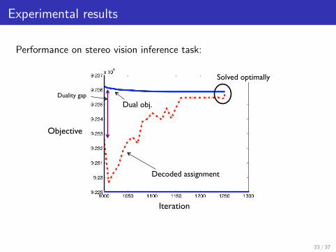
Experimental results

Performance on stereo vision inference task:

Decoded assignment!

Dual obj.!

Iteration!

Objective!

Solved optimally!

Duality gap!

33 / 37

Dual decomposition = basic LP relaxation

Recall we obtained the following dual linear program: L(δ) =∑

i∈Vmaxxi

(θi (xi ) +

∑

ij∈Eδj→i (xi )

)+∑

ij∈Emaxxi ,xj


),

DUAL-LP(θ) = minδ

L(δ)

We showed two ways of upper bounding the value of the MAPassignment:

MAP(θ) ≤ Basic LP(θ) (1)

MAP(θ) ≤ DUAL-LP(θ) ≤ L(δ) (2)

Although we derived these linear programs in seemingly very differentways, in turns out that:

Basic LP(θ) = DUAL-LP(θ) [SonGloJaa11]

The dual LP allows us to upper bound the value of the MAP assignmentwithout solving an LP to optimality

34 / 37

Linear programming duality

(Dual) LP relaxation!

MAP assignment!(Primal) LP relaxation!

�µ�

x*! Integer linear program!

MAP(θ) ≤ Basic LP(θ) = DUAL-LP(θ) ≤ L(δ)

35 / 37

Conclusion

LP relaxations yield a powerful approach for MAP inference

Naturally lead to

considerations of polytope or cutting planesdual decomposition and message passing

Close relationship to methods for marginal inference

Help build understanding as well as develop new algorithmic tools

Exciting current research

Thank you

36 / 37

References

V. Kolmogorov, J. Thapper, and S. Zivny. The power of linear programmingfor general-valued CSPs. SIAM Journal on Computing, 44(1):136, 2015.

S. Park and J. Shin. Max-product belief propagation for linear programming:applications to combinatorial optimization. In UAI, 2015.

D. Sontag. Approximate inference in graphical models using LP relaxations.PhD thesis, MIT, 2010.

D. Sontag, A. Globerson, and T. Jaakkola. Introduction to dual decompositionfor inference. In Optimization for Machine Learning, MIT Press, 2011.

J. Thapper and S. Zivny. The complexity of finite-valued CSPs. arxiv technicalreport, 2015. http://arxiv.org/abs/1210.2987v3

M. Wainwright and M. Jordan. Treewidth-based conditions for exactness ofthe Sherali-Adams and Lasserre relaxations. Univ. California, Berkeley,Technical Report, 671:4, 2004.

M. Wainwright and M. Jordan. Graphical models, exponential families andvariational inference. Foundations and Trends in Machine Learning,1(1-2):1305, 2008.

37 / 37

http://arxiv.org/abs/1210.2987v3

an introduction to lp relaxations for map inference

Documents