an introduction to many-body green’s func- tions in and

An introduction to many-body Green’s func-tions in and out of equilibrium

James K. FreericksDepartment of Physics, Georgetown UniversityReiss Science Building, 37th and O Sts. NW,Washington, DC 20057, U. S. A.

Contents1 Introduction 2

2 Green’s functions in equilibrium and the Lehmann representation 3

3 Green’s functions out of equilibrium and the “contour” 5

4 The self-energy and the equation of motion 7

5 Incorporating an external field and the issue of gauge invariance 8

6 Nonequilibrium dynamical mean-field theory 11

7 Numerical strategies to calculate the Green’s function 13

8 Examples 19

9 Conclusions 24

arX

iv:1

907.

1130

2v1

[co

nd-m

at.s

tr-e

l] 2

5 Ju

l 201

9

.2 James K. Freericks

1 Introduction

This chapter is all about Green’s functions. Many-body Green’s functions are a marvelous toolto employ in quantum-mechanical calculations. They require a rather large set of mathematicalmachinery to develop their theory and a sophisticated computational methodology to determinethem for anything but the simplest systems. But what do we really use them for? Essentially,there are two main uses: one is to compute the thermodynamic expectation value of c†c, whichallows us to determine all interesting single-particle expectation values, like the kinetic energy,the momentum distribution, etc. and two is to determine the many-body density of states, whichtells us how the quantum states are distributed in momentum and energy. In large dimensions,they can also be used to determine some two-particle correlation functions like the optical con-ductivity, because the vertex corrections vanish. It seems like this is a lot of work to end up withonly a few concrete results. But that is the way it is. No one has figured out any way to do thismore efficiently. If you determine how to, fame and fortune are likely to follow!

Before jumping into the full glory, we will give just a brief history. This is one that focuses onmy opinion of where critical ideas originated. It is not intended to be exhaustive or complete,and of course I may be wrong about where the different ideas came from. The equilibriumtheory for Green’s functions was developed primarily in the 1950s. The Lehmann represen-tation [1] was discovered in 1954. The Russian school developed much of the perturbativeapproach to Green’s functions, which is summarized in the monograph of Abrikosov, Gorkov,and Dzyaloshinski [2]. Joaquin Luttinger and John Ward developed a functional approach [3]and Matsubara determined how to solve for thermal Green’s functions [4]. But the reference Ilike the most for clarifying many-body Green’s functions both in and out of equilibrium is themonograph by Baym and Kadanoff [5]. Their approach is one we will follow, at least in spirit,in this chapter. Of course, Keldysh’s perpsective [6] was also important. Serious numerical cal-culations of Green’s functions (in real time and frequency) only began with the development ofdynamical mean-field theory in the 1990s [7]. The nonequilibrium generalization began only inthe mid 2000’s [8–10], but it was heavily influenced by earlier work from Uwe Brandt [11–13].

Now that we have set the stage for you as to where we are going, get ready for the ride. The the-ory is beautiful, logical, abstract, and complex. Mastering it is a key in becoming a many-bodytheorist. We begin in section 2 with a discussion of equilibrium Green’s functions focused onthe Lehmann representation. Section 3, generalizes and unifies the formalism to the contour-ordered Green’s function. Section 4 introduces the self-energy and the equation of motion.Section 5 illustrates how to include the external electric field. Section 6 introduces how onesolves these problems within the nonequilibrium dynamical mean-field theory approach. Nu-merics are discussed in section 7, followed by examples in section 8. We conclude in section9.

Many-body Green’s functions .3

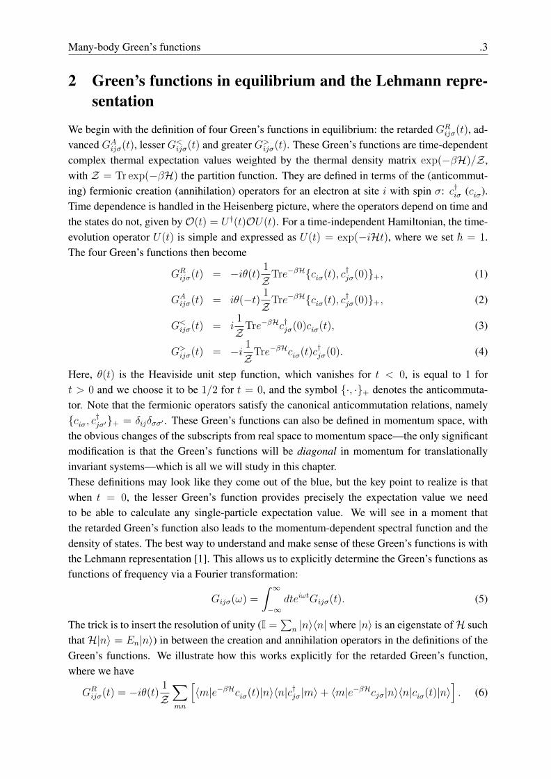
2 Green’s functions in equilibrium and the Lehmann repre-sentation

We begin with the definition of four Green’s functions in equilibrium: the retarded GRijσ(t), ad-

vanced GAijσ(t), lesser G<

ijσ(t) and greater G>ijσ(t). These Green’s functions are time-dependent

complex thermal expectation values weighted by the thermal density matrix exp(−βH)/Z ,with Z = Tr exp(−βH) the partition function. They are defined in terms of the (anticommut-ing) fermionic creation (annihilation) operators for an electron at site i with spin σ: c†iσ (ciσ).Time dependence is handled in the Heisenberg picture, where the operators depend on time andthe states do not, given byO(t) = U †(t)OU(t). For a time-independent Hamiltonian, the time-evolution operator U(t) is simple and expressed as U(t) = exp(−iHt), where we set ~ = 1.The four Green’s functions then become

GRijσ(t) = −iθ(t) 1

ZTre−βH{ciσ(t), c†jσ(0)}+, (1)

GAijσ(t) = iθ(−t) 1

ZTre−βH{ciσ(t), c†jσ(0)}+, (2)

G<ijσ(t) = i

1

ZTre−βHc†jσ(0)ciσ(t), (3)

G>ijσ(t) = −i 1

ZTre−βHciσ(t)c†jσ(0). (4)

Here, θ(t) is the Heaviside unit step function, which vanishes for t < 0, is equal to 1 fort > 0 and we choose it to be 1/2 for t = 0, and the symbol {·, ·}+ denotes the anticommuta-tor. Note that the fermionic operators satisfy the canonical anticommutation relations, namely{ciσ, c

†jσ′}+ = δijδσσ′ . These Green’s functions can also be defined in momentum space, with

the obvious changes of the subscripts from real space to momentum space—the only significantmodification is that the Green’s functions will be diagonal in momentum for translationallyinvariant systems—which is all we will study in this chapter.These definitions may look like they come out of the blue, but the key point to realize is thatwhen t = 0, the lesser Green’s function provides precisely the expectation value we needto be able to calculate any single-particle expectation value. We will see in a moment thatthe retarded Green’s function also leads to the momentum-dependent spectral function and thedensity of states. The best way to understand and make sense of these Green’s functions is withthe Lehmann representation [1]. This allows us to explicitly determine the Green’s functions asfunctions of frequency via a Fourier transformation:

Gijσ(ω) =

∫ ∞−∞

dteiωtGijσ(t). (5)

The trick is to insert the resolution of unity (I =∑

n |n〉〈n| where |n〉 is an eigenstate ofH suchthat H|n〉 = En|n〉) in between the creation and annihilation operators in the definitions of theGreen’s functions. We illustrate how this works explicitly for the retarded Green’s function,where we have


Z∑mn

[〈m|e−βHciσ(t)|n〉〈n|c†jσ|m〉+ 〈m|e−βHcjσ|n〉〈n|ciσ(t)|n〉

]. (6)


We now use the fact that these states are eigenstates ofH and the Heisenberg representation forthe time dependent operators to find

GRijσ(t) = −iθ(t)

∑mn

e−βEm

Z

[ei(Em−En)t〈m|ciσ|n〉〈n|c

†jσ|m〉+ e−i(Em−En)t〈m|c†jσ|n〉〈n|ciσ|m〉

].

(7)Next, we interchange m↔ n in the second term to give


Z∑mn

(e−βEm + e−βEn

)ei(Em−En)t〈m|ciσ|n〉〈n|c

†jσ|m〉. (8)

It is now time to do the Fourier transform. We achieve this by shifting ω → ω + i0+ to makethe integrand vanish at the large time limit, which finally results in

GRijσ(ω) =

1

Z∑mn

e−βEm + e−βEn

ω + Em − En + i0+〈m|ciσ|n〉〈n|c

†jσ|m〉. (9)

This is already of the form that we can discover some interesting things. If we recall the Diracrelation 1

ω+i0+ = Pω− iπδ(ω) (with P denoting the principal value), then we find the local

density of states via

Aiσ(ω) = − 1

πImGiiσ(ω) =

∑mn

δ(ω + Em − En)e−βEm + e−βEn

Z|〈m|ciσ|n〉|2. (10)

This density of states satisfies a sum rule. In particular,∫ ∞−∞

dωAiσ(ω) =1

Z∑n

e−βEn(ciσc

†iσ + c†iσciσ

)= 1, (11)

which follows from the anticommutation relation of the fermionic operators; note that you canalso see this directly by taking the limit t → 0+ in Eq. (1). This result holds in momentumspace too: the retarded Green’s function becomes

GRkσ(t) = −iθ(t) 1

ZTre−βH

{ckσ(t), c†kσ(t)

}+

(12)

GRkσ(ω) =

1

Z∑mn

e−βEm + e−βEn

ω + Em − En + i0+〈m|ckσ|n〉〈n|c

†kσ|m〉, (13)

with the operators being the momentum space operators, determined by a Fourier transformfrom real space:

ckσ =1

|Λ|∑j∈Λ

cjσe−ik·Rj and c†kσ =

1

|Λ|∑j∈Λ

cjσeik·Rj . (14)

Here, the lattice with periodic boundary conditions is denoted by Λ = {Ri} and |Λ| is thenumber of lattice sites in the system. We usually do not use a bold font for the momentumlabel in the subscript of the creation or annihilation operator; one should be able to figure out


from the context whether we are working in real space or momentum space. The momentum-space Green’s functions have a similarly defined spectral function Akσ(k, ω) = −ImGR

kσ(ω)/π,which also satisfies a sum rule given by the integral over all frequency being equal to one. Onecan easily show that the advanced Green’s function in frequency space is equal to the Hermitianconjugate of the retarded Green’s function, because we need to shift ω → ω − i0+ to controlthe integrand at the lower limit. Hence, we have GA

ijσ(ω) = GR∗jiσ(ω).

We also sketch how the calculation works for the lesser and greater Green’s functions. Here,we have to control the integrand at both endpoints of the integral. To do so, we split it at 0and introduce the appropriate infinitesimal convergence factor in each piece. The rest of thecalculation proceeds as above and one finds that the two pieces have their imaginary parts add,so we finally obtain:

G<ijσ(ω) = 2iπ

1

Z∑mn

δ(ω + Em − En)e−βEn〈m|ciσ|n〉〈n|c†jσ|m〉. (15)

The greater Green’s function similarly becomes

G>ijσ(ω) = −2iπ

1

Z∑mn

δ(ω + Em − En)e−βEm〈m|ciσ|n〉〈n|c†jσ|m〉. (16)

Note that we can use the delta function to immediately infer an important identity, namelythat G<

ijσ(ω) = − exp(−βω)G>ijσ(ω). Combining this result with the fact that ImGR

ijσ(ω) =

Im[G<ijσ(ω)−G>

ijσ(ω)]/2, we finally learn that

G<ijσ(ω) = −2if(ω)ImGR

ijσ(ω) and G>ijσ(ω) = 2i[1− f(ω)]ImGR

ijσ(ω). (17)

This equilibrium relationship is sometimes called the fluctuation-dissipation theorem.

3 Green’s functions out of equilibrium and the “contour”

−iβ

tmax

−∞(a)

−∞

(b)tmax −iβ−∞ −∞−∞

Fig. 1: (a) Kadanoff-Baym-Keldysh contour used in the contruction of the contour-orderedGreen’s function. The contour starts at −∞, runs out to the maximum of t and t′, runs backto −∞ and then runs parallel to the imaginary axis for a distance equal to β. (b) The con-tour can be “stretched” into a straight line as indicated here, which is convenient for properlyimplementing time-ordering along the contour.


Now we move onto nonequilibrium where the Hamiltonian is time-dependent H(t). The evo-lution operator depends on two times and becomes U(t, t′) = Tt exp

[−i∫ tt′dtH(t)

]. It sat-

isfies the semigroup property U(t, t′′)U(t′′, t′) = U(t, t′), with U(t, t) = I and i∂tU(t, t′) =

H(t)U(t, t′). The Green’s functions in nonequilibrium are defined by the same equations asbefore, namely Eqs. (1–4), except now they depend on two times, with t′ being the argument ofthe c† operator. All of these Green’s functions require us to evaluate one of two matrix elements.We examine one of them here and assume t > t′ for concreteness:

1

ZTre−βHciσ(t)c†jσ(t′) =

1

ZTre−βHU †(t,−∞)ciσU(t,−∞)U †(t′,−∞)c†jσU(t′,−∞) (18)

=1

ZTre−βHU(−∞, t)ciσU(t, t′)c†jσU(t′,−∞) (19)

where we used the facts that U †(t1, t2) = U(t2, t1) and the semigroup property to show thatU(t,−∞)U †(t′,−∞) = U(t, t′). The time-evolution operators, including time evolution inthe imaginary axis direction for the exp(−βH) term, can be seen to all live on the so-calledKadanoff-Baym-Keldysh contour, which is shown in Fig. 1. Starting with time at −∞, weevolve forward to t′, then apply the c†, evolve forward to time t, apply the c operator, andthen evolve backwards in time to −∞. The lesser and greater Green’s functions are easilydetermined in this fashion. The retarded or advanced Green’s functions can then be foundby taking the appropriate differences of greater and lesser functions with the convention thatt > t′ for the retarded case and t < t′ for the advanced case. Now that we have these Green’sfunctions, we can generalize the definition of the Green’s function to allow both times to lieanywhere on the contour. We take the time-ordered Green’s function, with the time-orderingtaking place along the contour, and we call it the contour-ordered Green’s function:

Gcijσ(t, t′) =

−i 1ZTre−βH ciσ(t)c†jσ(t′) for t >c t

′

i 1ZTre−βH c†jσ(t′)ciσ(t) for t <c t

′.

, (20)

where the c subscript on the less than or greater than symbol is to denote whether one time isahead of or behind the other on the contour, regardless of the numerical values of t and t′. ThisGreen’s function is the workhorse of nonequilibrium many-body physics—we use it to calculateanything that can be calculated with the single-particle Green’s functions.Note that in these lectures, we will work with the contour-ordered Green’s function itself, whichis a continuous matrix operator in time. In many other works, the Green’s function is furtherdecomposed into components where the times lie on the same or different branches of the realcontour (2× 2 matrix) [6] or of the two real and one imaginary branches of the contour (3× 3

matrix) [14]. In the 3 × 3 case, one has real, imaginary and mixed Green’s functions, the lastones determining the so-called initial correlations. In the 2× 2 case, it is common to transformthe matrix to make it upper triangular, expressing the retarded, advanced and so-called KeldyshGreen’s functions. In general, I find that these decompositions and transformations make thematerial more difficult than it actually is and it is best to defer using them until one has gainedsome mastery of the basics. Here, we will work solely with the contour-ordered functions.


4 The self-energy and the equation of motion

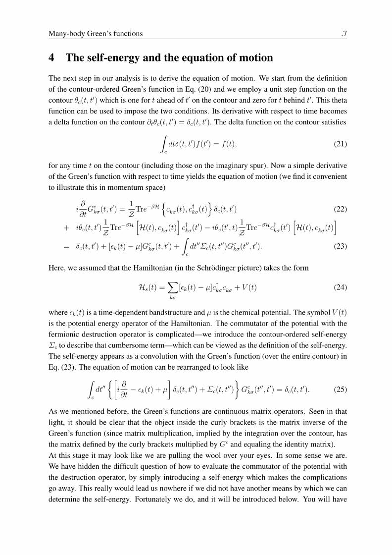
The next step in our analysis is to derive the equation of motion. We start from the definitionof the contour-ordered Green’s function in Eq. (20) and we employ a unit step function on thecontour θc(t, t′) which is one for t ahead of t′ on the contour and zero for t behind t′. This thetafunction can be used to impose the two conditions. Its derivative with respect to time becomesa delta function on the contour ∂tθc(t, t′) = δc(t, t

′). The delta function on the contour satisfies∫c

dtδ(t, t′)f(t′) = f(t), (21)

for any time t on the contour (including those on the imaginary spur). Now a simple derivativeof the Green’s function with respect to time yields the equation of motion (we find it convenientto illustrate this in momentum space)

i∂

∂tGckσ(t, t′) =

1

ZTre−βH

{ckσ(t), c†kσ(t)

}δc(t, t

′) (22)

+ iθc(t, t′)

1

ZTre−βH

[H(t), ckσ(t)

]c†kσ(t′)− iθc(t′, t)

1

ZTre−βHc†kσ(t′)

[H(t), ckσ(t)

]= δc(t, t

′) + [εk(t)− µ]Gckσ(t, t′) +

∫c

dt′′Σc(t, t′′)Gc

kσ(t′′, t′). (23)

Here, we assumed that the Hamiltonian (in the Schrodinger picture) takes the form

Hs(t) =∑kσ

[εk(t)− µ]c†kσckσ + V (t) (24)

where εk(t) is a time-dependent bandstructure and µ is the chemical potential. The symbol V (t)

is the potential energy operator of the Hamiltonian. The commutator of the potential with thefermionic destruction operator is complicated—we introduce the contour-ordered self-energyΣc to describe that cumbersome term—which can be viewed as the definition of the self-energy.The self-energy appears as a convolution with the Green’s function (over the entire contour) inEq. (23). The equation of motion can be rearranged to look like∫

c

dt′′{[

i∂

∂t− εk(t) + µ

]δc(t, t

′′) +Σc(t, t′′)

}Gckσ(t′′, t′) = δc(t, t

′). (25)

As we mentioned before, the Green’s functions are continuous matrix operators. Seen in thatlight, it should be clear that the object inside the curly brackets is the matrix inverse of theGreen’s function (since matrix multiplication, implied by the integration over the contour, hasthe matrix defined by the curly brackets multiplied by Gc and equaling the identity matrix).At this stage it may look like we are pulling the wool over your eyes. In some sense we are.We have hidden the difficult question of how to evaluate the commutator of the potential withthe destruction operator, by simply introducing a self-energy which makes the complicationsgo away. This really would lead us nowhere if we did not have another means by which we candetermine the self-energy. Fortunately we do, and it will be introduced below. You will have


to wait to see how that fits in. All of the challenge in many-body physics boils down to thisquestion of “how can we calculate the self-energy?”Now is also a good time to discuss the issue of how do we work with these complicated ob-jects? If you look carefully, you will see we are working with matrices. Admittedly they arecontinuous matrix operator equations, but like any continuous object, we discretize them whenwe want to work with them on a computer. And indeed, that is what we will do here whenwe describe the DMFT algorithm below. We always extrapolate the discretization to zero torecover the continuous matrix operator results. It is important to recognize these facts now, as itwill make your comfort level with the approach much higher as we develop the subject further.

5 Incorporating an external field and the issue of gauge in-variance

I always found it odd in dealing with fields in quantum mechanics to learn that we do not alwaysrespect Maxwell’s equations. This should not come as a surprise to you, because Maxwell’sequations are relativistically invariant, and quantum mechanics only becomes relativisticallyinvariant with a properly constructed relativistic quantum field theory. Nevertheless, we chooseto neglect even more aspects of Maxwell’s equations than just relativistic invariance. Thisbecomes necessary because the quantum problem cannot be solved unless we do this (and,fortunately, the neglected terms are small).The main issue we face is that we want the field to be spatially uniform but time varying.Maxwell says such fields do not exist, but we press on anyway. You see, a spatially uniformfield means that I still have translation invariance and that is needed to make the analysis simpleenough that it can be properly carried out. We justify this in part because optical wavelengthsare much larger than lattice spacings and because magnetic field effects are small due the extra1/c factors multiplying them. Even with this simplification, properly understanding how tointroduce a large amplitude electric field is no easy task.The field will be described via the Peierls’ substitution [15]. This is accomplished by shiftingk → k − eA(t), which becomes k + eEt, for a constant (dc) field. This seems like the rightthing to do, because it parallels the minimal substitution performed in single-particle quantummechanics when incorporating an electric field, but we have to remember that we are nowworking with a system projected to the lowest lying s-orbital band, so it may not be obviousthat this remains the correct thing to do. Unfortunately, there is no rigorous proof that this resultis correct, but one can show that if we work in a single band (neglecting interband transitions)and have inversion symmetry in the lattice, then the field generated by a scalar potential, andthe field generated by the equivalent vector potential will yield identical noninteracting Green’sfunctions [16]. We then assume that adding interactions to the system does not change thiscorrespondence, so we have an approach that is exact for a single-band model. One should bearin mind that there may be subtle issues with multiple bands and the question of how to preciselywork with gauge-invariant objects in mutliband models has not been completely resolved yet.


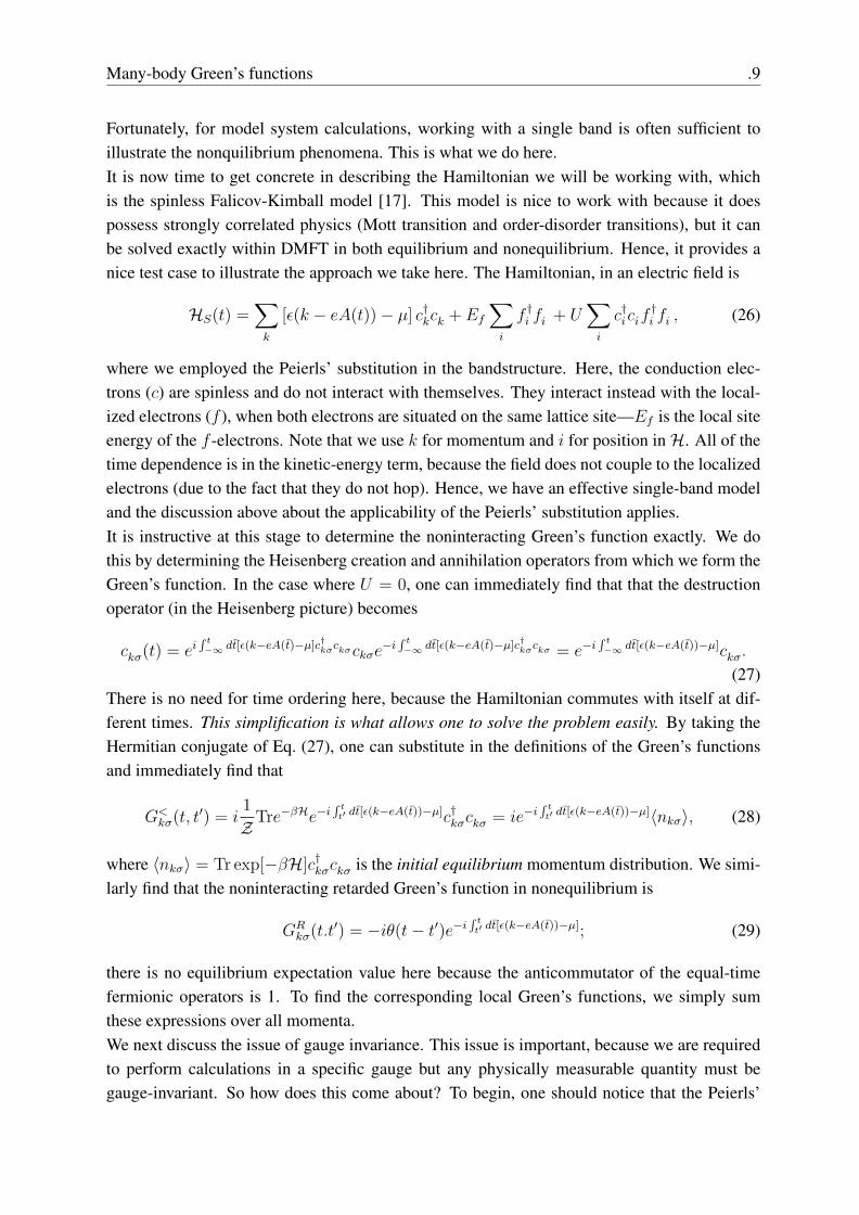
Fortunately, for model system calculations, working with a single band is often sufficient toillustrate the nonquilibrium phenomena. This is what we do here.It is now time to get concrete in describing the Hamiltonian we will be working with, whichis the spinless Falicov-Kimball model [17]. This model is nice to work with because it doespossess strongly correlated physics (Mott transition and order-disorder transitions), but it canbe solved exactly within DMFT in both equilibrium and nonequilibrium. Hence, it provides anice test case to illustrate the approach we take here. The Hamiltonian, in an electric field is

HS(t) =∑k

[ε(k − eA(t))− µ] c†kck + Ef∑i

f †i fi + U∑i

c†icif†i fi , (26)

where we employed the Peierls’ substitution in the bandstructure. Here, the conduction elec-trons (c) are spinless and do not interact with themselves. They interact instead with the local-ized electrons (f ), when both electrons are situated on the same lattice site—Ef is the local siteenergy of the f -electrons. Note that we use k for momentum and i for position inH. All of thetime dependence is in the kinetic-energy term, because the field does not couple to the localizedelectrons (due to the fact that they do not hop). Hence, we have an effective single-band modeland the discussion above about the applicability of the Peierls’ substitution applies.It is instructive at this stage to determine the noninteracting Green’s function exactly. We dothis by determining the Heisenberg creation and annihilation operators from which we form theGreen’s function. In the case where U = 0, one can immediately find that that the destructionoperator (in the Heisenberg picture) becomes

ckσ(t) = ei∫ t−∞ dt[ε(k−eA(t)−µ]c†kσckσckσe

−i∫ t−∞ dt[ε(k−eA(t)−µ]c†kσckσ = e−i

∫ t−∞ dt[ε(k−eA(t))−µ]ckσ.

(27)There is no need for time ordering here, because the Hamiltonian commutes with itself at dif-ferent times. This simplification is what allows one to solve the problem easily. By taking theHermitian conjugate of Eq. (27), one can substitute in the definitions of the Green’s functionsand immediately find that

G<kσ(t, t′) = i

1

ZTre−βHe−i

∫ tt′ dt[ε(k−eA(t))−µ]c†kσckσ = ie−i

∫ tt′ dt[ε(k−eA(t))−µ]〈nkσ〉, (28)

where 〈nkσ〉 = Tr exp[−βH]c†kσckσ is the initial equilibrium momentum distribution. We simi-larly find that the noninteracting retarded Green’s function in nonequilibrium is

GRkσ(t.t′) = −iθ(t− t′)e−i

∫ tt′ dt[ε(k−eA(t))−µ]; (29)

there is no equilibrium expectation value here because the anticommutator of the equal-timefermionic operators is 1. To find the corresponding local Green’s functions, we simply sumthese expressions over all momenta.We next discuss the issue of gauge invariance. This issue is important, because we are requiredto perform calculations in a specific gauge but any physically measurable quantity must begauge-invariant. So how does this come about? To begin, one should notice that the Peierls’


substitution guarantees that any quantity that is local, like the current, is gauge invariant, be-cause the sum over all momenta includes every term, even if the momenta are shifted due tothe Peierls substitution. Momentum-dependent quantities, however, appear to depend directlyon the vector potential. To properly formulate a gauge-invariant theory requires us to go backand formulate the problem (using a complete basis set, not a single-band downfolding) prop-erly to illustrate the gauge-invariant nature of the observables. No one has yet been able to dothis for a system with a nontrivial bandstructure. For a single-band model, we instead directlyenforce gauge invariance using the so-called gauge-invariant Green’s functions, introduced byBertoncini and Jauho [18]. These Green’s functions are constructed to be manifestly gaugeinvariant—the change in the phase of the creation and destruction operators is chosen to pre-cisely cancel the change in the phase from the gauge transformation. We determine them inmomentum space by making a shift

k → k(t, t′) = k +

∫ 12

− 12

dλA

(t+ t′

2+ λ(t− t′)

). (30)

Note that one needs to be careful in evaluating this integral in the limit as t → t′. In this limit,we find k → k + A(t). The explicit formula for the gauge-invariant Green’s function, whichuses a tilde to denote that it is gauge-invariant, is

Gkσ(t, t′) = Gk(t,t′)σ(t, t′). (31)

The demonstration of the gauge-invariance is given in Ref. [18]. Note that the local Greensfunctions are always manifestly gauge-invariant because the map k → k(t, t′) is a “one-to-oneand onto” map for any fixed set of times.We end this section with a discussion of the current operator and how it is related to gaugeinvariance. The current operator is calculated in a straightforward way via the commutator ofthe Hamiltonian with the charge polarization operator. We do not provide the details here, butsimply note that they can be found in most many-body physics textbooks. The end result is that

j =∑σ

∑k

vkc†kσckσ. (32)

Here, we have the band velocity is given by vk = ∇εk. The gauge-invariant form of the expec-tation value for the current is then

〈j〉 = −i∑σ

∑k

vkG<kσ(t, t). (33)

We can re-express in terms of the original Green’s functions, by shifting k → k − A(t). Thisyields the equivalent formula

〈j〉 = −i∑σ

∑k

vk−A(t)G<kσ(t, t). (34)

As you can easily see, these two results are identical by simply performing a uniform shift of themomentum in the summation. Generically, this is how different expectation values behave—in


the gauge-invariant form, one evaluates them the same as in linear response, but uses the gauge-invariant Green’s functions, while in the non-gauge-invariant form, one evaluates in a formsimilar to linear response, but appropriately shifts the momentum in the terms that multiply theGreen’s functions (which is a beyond-linear-response “correction”).

6 Nonequilibrium dynamical mean-field theory

The premise of dynamical mean-field theory (DMFT) is that the self-energy of an impurity inan appropriately chosen time-dependent field is the same as the self-energy on the lattice. Ingeneral, we know this cannot be true, because the lattice self-energy depends on momentum,and hence is not local. But, if we choose the hopping matrix elements to scale like t = t∗/2

√d

for a d-dimensional lattice, then one can rigorously show that in the limit d → ∞, the self-energy does indeed become local [19]. So, in this limit, the DMFT assumption holds and itprovides another limiting case where one can exactly solve the many-body problem (the otherlimit being that of d = 1).The physical picture to keep in mind, for DMFT, is to think of looking at what happens just ona single site of the lattice. As a function of time, we will see electrons hop onto and off of thesite. If we can adjust the time-dependent field for the impurity in such a way that it producesthe same behavior in time on the impurity, then the impurity site will look like the lattice. Thismotivates the following iterative algorithm [20] to solve these models: (1) Begin with a guessfor the self-energy (Σ = 0 often works); (2) sum the momentum-dependent Green’s functionover all momentum to determine the local Green’s function

Gciiσ(t, t′) =

∑k

{[Gc

kσ(U=0)]−1 −Σ}−1

t,t′, (35)

with Gckσ(U=0) the noninteracting momentum-dependent contour-ordered Green’s function on

the lattice and the subscript denoting the t, t′ element of the matrix inverse) ; (3) Use Dyson’sequation to determine the effective medium G0 via

[Gc0σ]−1

t,t′ = [Gciiσ]−1

t,t′ +Σc(t, t′); (36)

(4) solve the impurity problem in the extracted effective medium (which determines the timeevolution on the impurity); (5) extract the self-energy for the impurity using an appropriatelymodified Eq. (36); and (8) repeat steps (2–7) until the self-energy has converged to the desiredlevel of accuracy. The difference from the conventional iterative DMFT algorithm is that theobjects worked with are now continuous matrix operators in time rather than simple functions offrequency. Sometimes this creates a roadblock for students to follow how the algorithm works,but there is no reason why it should. Finally, we note that because each inverse of a Green’sfunction here implies a matrix inversion, we will want to organize the calculation in such a wayas to minimize the inversions. This will be explained in more detail when we discuss numericalimplementations below.


One of the simplifications in equilibrium DMFT is that the fact that the self-energy has no mo-mentum dependence allows us to perform the summation over momentum via a single integralover the noninteracting density of states. Things are not quite as simple for the nonequilibriumcase, as we now discuss. The bandstructure for a hypercubic lattice in d→∞ is given by

εk = − limd→∞

t∗√d

d∑i=1

cos(ki). (37)

The central limit theorem tells us that εk is distributed according to a Gaussian distribution via

ρ(ε) =1√πt∗

e−ε2

. (38)

In nonequilibrium, we have a second band energy to work with

εk = − limd→∞

t∗√d

d∑i=1

sin(ki), (39)

because the Peierls substitution shifts cos(ki) → cos(ki) cos(Ai(t)) + sin(ki) sin(Ai(t)). Thejoint density of states becomes the product of two Gaussians, given by

ρ(ε, ε) =1

πt∗2e−

ε2

t∗2− ε2

t∗2 . (40)

This second band energy can be thought of as the projection of the band velocity onto thedirection of the electric field. Hence, the computation of the local Green’s function in step(2) is complicated by requiring a two-dimensional integration rather than a one-dimensionalintegration. This does make the numerics require significant additional resources, especiallybecause the integrands are matrix-valued.The most challenging part of the algorithm is step (4)—solving the impurity problem in nonequi-librium. Unfortunately, there are few techniques available to do this. Monte Carlo methodssuffer from the so-called phase problem, which might be able to be tamed using expansionsabout a perturbative solution and restricting updates to be nearly local in time via the inchwormalgorithm [21]. The other choice is perturbation theory either in the interaction (which oftendoes not work so well, except for electron-phonon coupling) or the hybridization of the impu-rity model (which works well at half filling). Here, we make a different choice, and choose asimplified model that can be solved exactly, the so-called spinless Falicov-Kimball model [17]:

H =∑ij

tijc†icj − µ

∑i

c†ici + Ef∑i

f †i fi + U∑i

c†icif†i fi . (41)

This model involves the interaction of conduction electrons (c) and localized electrons (f ). Theconduction electrons can hop on the lattice (we usually take the hopping only between nearestneighbors on a hypercubic lattice in the d → ∞ limit) and have a chemical potential µ. Thelocalized electrons have a site energy Ef . Both electrons interact with an on-site interaction U .The Falicov-Kimball model describes a rich set of physics, but it should not be viewed as aparadigm for all strongly correlated electrons. This is because it has some aspects that are not


seen in more common models like the Hubbard model. For example, it is never a Fermi liquidwhen U 6= 0, the conduction electron density of states is independent of temperature in thenormal state, and it is never a superconductor. But, it does display a lot of rich physics includinga Mott metal-insulator transition, ordered charge-density-wave phases at low temperature andeven phase separation when the densities of the two species are far enough apart. In addition, thef -electron density of states does exhibit strong temperature dependence, as expected in stronglycorrelated systems. It also displays orthogonality catastrophe behavior. The main interest in thenonequilibrium context has focused on the fact that it has a Mott transition. The most importantaspect of the model is that it can be solved exactly within DMFT—both in equilibrium and innonequilibrium.We will not go through the details of the equation of motion for the Green’s functions in theFalicov-Kimball model to show how one can solve it. The procedure is most efficiently per-formed using a path-integral formulation because the time-dependent field on the impurity can-not be easily expressed in terms of a Hamiltonian (unless one introduces a bath for the impuritywhich does this). Instead, one can employ functional methods to exactly compute the functionalderivative of the partition function with respect to the dynamical mean-field, which then is em-ployed to extract the Green’s function. Then, because the f -electron number is conserved in themodel, we obtain the Green’s function of the impurity by summing over appropriately weightedcombinations of the solution with no f -electrons and with one f -electron. The end result isthat the impurity Green’s function for the Falicov-Kimball model in an effective medium is thefollowing:

Gc0(t, t′) = (1− w1)Gc

0(t, t′) + w1

[(Gc

0)−1 − UI]−1

t,t′. (42)

The symbol w1 = 〈f †f〉 is the filling of the localized electrons (per lattice site). Since the f -electron number operator commutes with H, the localized electron number is a constant of themotion and does not change with time, even in the presence of large electric fields. Note thatwe will work at half-filling where the electron densities for the conduction electrons and thelocalized electrons are each equal to 1/2. This point corresponds to µ = U/2 and Ef = −U/2.Details not presented here can be found in the original literature [8, 9].

7 Numerical strategies to calculate the Green’s function

Now we need to sort out just how we put this algorithm on a computer and implement it. Thisdiscussion closely follows Ref. [9]. As mentioned above, the challenge is that we are workingwith continuous matrix operators, with integration over the contour corresponding to matrixmultiplication of these operators. Such objects cannot be directly put onto a computer. Instead,we have to first discretize the problem, replacing the continuous operators by discrete matrices.There are a few subtle points that are involved corresponding to the integration measure overthe contour when we do this, but we will precisely describe how we achieve this below. Inorder to recover the results for the continuous matrix operators, we need to extrapolate thediscretized results to the limit where the discretization size goes to zero. This is done in the


most mundane way possible—simply repeat the calculation for a number of different ∆t valuesand use Lagrange interpolation as an extrapolation formula to the ∆t → 0 limit. We finallycheck sum rules of the data to verify that the extrapolation procedure worked properly. Detailsfollow.We first need to be concrete about how the discretization is performed. This involves Nt pointson the upper real branch (ranging from tmin to tmax −∆t), Nt points on the lower real branch(ranging from tmax to tmin + ∆t), and 100 points along the imaginary axis (ranging from tminto tmin − iβ + 0.1i, with β = 10); hence ∆t = (tmax − tmin)/Nt. We often find that fixingthe number of points on the imaginary time branch rather than scaling them in the same fashionas on the real axis does not cause any significant errors, but it allows the calculations to beperformed with fewer total number of points. The discrete time values on the contour become

tj = −tmin + (j − 1)∆t, 1 ≤ j ≤ Nt, (43)

= tmax − (j −Nt − 1)∆t, Nt + 1 ≤ j ≤ 2Nt,

= tmin − 0.1i(j − 2Nt − 1), 2Nt + 1 ≤ j ≤ 2Nt + 100,

where we used the fact that the discretization along the imaginary axis is always fixed at ∆τ =

0.1 in our calculations (and we pick the initial temperature to be T = 0.1t∗ or β = 10). Weuse a leftpoint rectangular integration rule for discretizing integrals over the contour, which isimplemented as follows: ∫

c

dtf(t) =2Nt+100∑i=1

Wif(ti), (44)

where the weights satisfy

Wj = ∆t, 1 ≤ j ≤ Nt,

= −∆t, Nt + 1 ≤ j ≤ 2Nt,

= −0.1i, 2Nt + 1 ≤ j ≤ 2Nt + 100. (45)

The leftpoint integration rule evaluates the function at the “earliest” point (in the sense of timeordering along the contour, see Fig. 1) in the time interval that has been discretized for thequadrature rule (which is the left hand side of the interval when we are on the upper real branchand right hand side when we are on the lower real time branch).One of the important aspects of many-body Green’s functions is that they satisfy a boundarycondition. This is what determines whether the Green’s function is bosonic or fermionic. Forexample, you should already be familiar with the fact that the thermal Green’s functions areantiperiodic on the imaginary time axis. The contour-ordered Green’s function also satisfiesa boundary condition where we identify the points tmin with tmin − iβ. One can show fromthe definition of the contour-ordered Green’s function and the invariance of the trace with re-spect to the ordering of operators that Gc

iiσ(tmin, t′) = −Gc

iiσ(tmin − iβ, t′) and Gciiσ(t, tmin) =

−Gciiσ(t, tmin − iβ). The proof is identical to how it is done for the thermal Green’s functions.

It involves cyclically moving a creation operator from the left to the right and commuting the


e−βH term through it which employs the fact that a cyclic permutation of elements in the productof a trace does not change the value of the trace.The delta function changes sign along the negative real time branch, and is imaginary alongthe last branch of the contour in order to satisfy the property that

∫cdt′δc(t, t

′)f(t′) = f(t). Inaddition, we find that the numerics work better if the definition of the delta function is done via“point splitting” (when we calculate the inverse of a Green’s function) so that the delta functiondoes not lie on the diagonal, but rather on the first subdiagonal matrix (in the limit as ∆t → 0

it becomes a diagonal operator). Because we identify the times tmin and tmin − iβ, the pointsplitting approach to the definition of the delta function allows us to incorporate the correctboundary condition into the definition of the discretized delta function. Hence, we define thediscretized delta function in terms of the quadrature weights, in the following way

δc(ti, tj) =1

Wi

δij+1, for integration over j, (46)

=1

Wi−1

δij+1, for integration over i, (47)

where ti and tj are two points on the discretized contour as described in Eq. (43), and Wi

are the quadrature weights described in Eq. (45). We have a different formula for integrationover the first variable versus integration over the second variable because we are using theleftpoint quadrature rule. Note that the formulas in Eqs. (46) and (47) hold only when i 6=1. When i = 1, the only nonzero matrix element for the discretized delta function is the1, j = 2Nt + 100 matrix element, and it has a sign change due to the boundary condition thatthe Green’s function satisfies. The discretization of the derivative of the delta function on thecontour is more complex. It is needed to determine the inverse of the Gc

0 for the impurity.The derivative is calculated by a two-point discretization that involves the diagonal and the firstsubdiagonal. Since all we need is the discrete representation of the operator [i∂ct + µ]δc(t, t

′),we summarize the discretization of that operator as follows

[i∂t + µ]δc(tj, tk) = i1

Wj

Mjk1

Wk

, (48)

with the matrix Mjk satisfying

Mjk =

1 0 0 ... 1+i∆tµ−1−i∆tµ 1 0 ... 0

0 −1−i∆tµ 1 0

. . .0 −1+i∆tµ 1 0

0 −1+i∆tµ 1

. . .−1−∆τµ 1

. . .−1−∆τµ 1

; (49)

here ∆τ = 0.1. The top third of the matrix corresponds to the upper real branch, the middlethird to the lower real branch and the bottom third to the imaginary branch. Note that theoperator [i∂ct + µ]δc is the inverse operator of the Green’s function of a spinless electron with a


chemical potential µ. Hence the determinant of this operator must equal the partition function ofa spinless electron in a chemical potential µ, namely 1+exp[βµ]. This holds because detG−1

non =

Znon for noninteracting electrons. Taking the determinant of the matrix Mjk (by evaluating theminors along the top row) gives

detM = 1 + (−1)2Nt+Nτ (1 + i∆tµ)(−1− i∆tµ)Nt−1

× (−1 + i∆tµ)Nt(−1−∆τµ)Nτ ,

≈ 1 + (1 +∆τµ)Nτ +O(∆t2), (50)

which becomes 1 + exp[βµ] in the limit where ∆t,∆τ → 0 (Nτ is the number of discretizationpoints on the imaginary axis). This shows the importance of the upper right hand matrix elementof the operator, which is required to produce the correct boundary condition for the Green’sfunction. It also provides a check on our algebra. In fact, we chose to point-split the deltafunction when we defined it’s discretized matrix operator precisely to ensure that this identityholds.We also have to show how to discretize the continuous matrix operator multiplication and how tofind the discretized approximation to the continuous matrix operator inverse. As we mentionedabove, the continuous matrix operator is described by a number for each entry i and j in thediscretized contour. We have to recall that matrix multiplication corresponds to an integral overthe contour, so this operation is discretized with the integration weights Wk as follows∫

c

dtA(t, t)B(t, t′) =∑k

A(ti, tk)WkB(tk, tj). (51)

Thus we must multiply the columns (or the rows) of the discrete matrix by the correspondingquadrature weight factors when we define the discretized matrix. This can be done either to thematrix on the left (columns) or to the matrix on the right (rows). To calculate the inverse, werecall the definition of the inverse for the continuous matrix operator∫

c

dtA(t, t)A−1(t, t′) = δc(t, t′), (52)

which becomes the following∑k

A(ti, tk)WkA−1(tk, tj) =

1

Wi

δij, (53)

in its discretized form. Note that we do not need to point-split the delta function here. Hence,the inverse of the matrix is found by inverting the matrix WiA(ti, tj)Wj , or, in other words, wemust multiply the rows and the columns by the quadrature weights before using conventionallinear algebra inversion routines to find the discretized version of the continuous matrix operatorinverse. This concludes the technical details for how to discretize and work with continuousmatrix operators.The next technical aspect we discuss is how to handle the calculation of the local Green’sfunction. Since the local Green’s function is found from the following equation:

Gcii(t, t

′) =1

πt∗2

∫dε

∫dε e−

ε2

t∗2− ε2

t∗2

[(I−Gc,non

ε,ε Σc)−1

Gc,nonε,ε

]t,t′

(54)


with the noninteracting Green’s function discussed earlier and given by

Gc,nonε,ε (t, t′) = i [f(ε− µ)− θc(t, t′)] e−i

∫ tt′ dt[cos(A(t))ε−sin(A(t))ε]. (55)

Note that we must have A(t) = 0 before the field is turned on. Of course an optical pumppulse also requires

∫∞−∞A(t)dt = 0, because a traveling electromagnetic wave has no dc field

component. We did not compute the matrix inverse of the noninteracting Green’s functionbecause re-expressing the formula in the above fashion makes the computation more efficient(because matrix multiplication requires less operations than a matrix inverse does).This step is the most computationally demanding step because we are evaluating the doubleintegral of a matrix-valued function and we need to compute one matrix inverse for each inte-grand. Fortunately, the computation for each (ε, ε) pair is independent of any other pair, so wecan do this in parallel with a master-slave algorithm. In the master-slave algorithm, one CPUcontrols the computation, sending a different (ε, ε) pair to each slave to compute its contributionto the integral and then accumulating all results. The sending of the pairs to each slave is simple.One has to carefully manage the sending of the results back to the master, because the data is alarge general complex matrix and they are all being received by one node. This is precisely thesituation where a communication bottleneck can occur.In order to use as few integration points as possible, we employ Gaussian integration, becausethe bare density of states for both the ε and the ε integrals is a Gaussian. We found it moreefficient to average the results with two consecutive numbers of points in the Gaussian inte-gration (like 100 and 101) instead of just using 200 points (which would entail twice as muchcomputation).The rest of the DMFT loop requires serial operations and is performed on the master to reducecommunications. One does have to pay attention to convergence. In metallic phases, and withstrong fields, the code will converge quickly But when the field is small or the interactionslarge, one might not be able to achieve complete convergence. Often the data is still good,nevertheless. One also should not make the convergence criterion too stringent. Usually 4digits of accuracy is more than enough for these problems. In most cases, one will need toiterate as many as 50-100 times for hard cases. But many results can be obtained with teniterations or less.Finally, one has to repeat the calculations for different discretizations and extrapolate to the∆t→ 0 limit. In order to use as much data as possible, it is best to first use a shape-preservingAkima spline to put all data on the same time grid and then use Lagrange interpolation as anextrapolation method to the ∆t → 0 limit. It is critical that one employs a shape-preservingspline, otherwise it will ruin your results. In addition, we find quadratic extrapolation usuallyworks best, but sometimes had to look at higher-order extrapolations. It is best to extrapolatethe data after the desired quantity has been determined as a function of t for all times on thegrid. For example, one would first determine the current by using the lesser Green’s functionand summing over all momentum for each time and then extrapolate the final current values asa function of time instead of extrapolating the Green’s functions, since doing the latter requiresa two-dimensional Lagrange extrapolation formula and uses large amounts of memory.


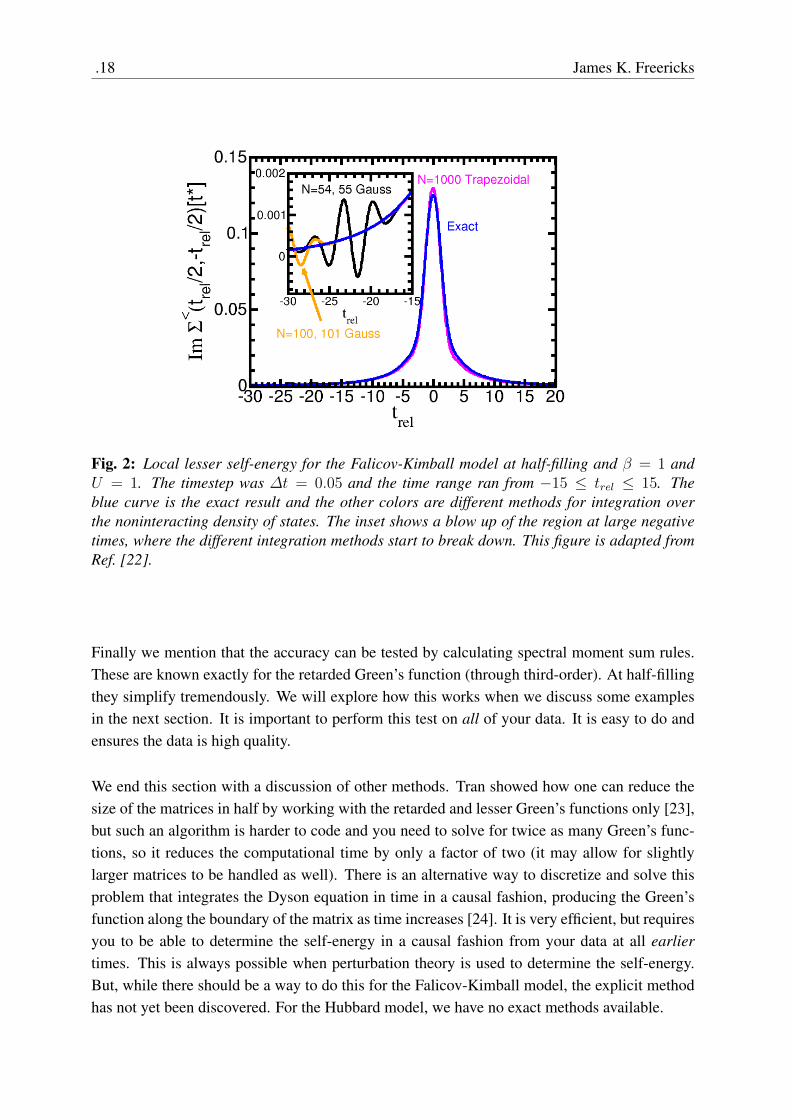
Fig. 2: Local lesser self-energy for the Falicov-Kimball model at half-filling and β = 1 andU = 1. The timestep was ∆t = 0.05 and the time range ran from −15 ≤ trel ≤ 15. Theblue curve is the exact result and the other colors are different methods for integration overthe noninteracting density of states. The inset shows a blow up of the region at large negativetimes, where the different integration methods start to break down. This figure is adapted fromRef. [22].

Finally we mention that the accuracy can be tested by calculating spectral moment sum rules.These are known exactly for the retarded Green’s function (through third-order). At half-fillingthey simplify tremendously. We will explore how this works when we discuss some examplesin the next section. It is important to perform this test on all of your data. It is easy to do andensures the data is high quality.

We end this section with a discussion of other methods. Tran showed how one can reduce thesize of the matrices in half by working with the retarded and lesser Green’s functions only [23],but such an algorithm is harder to code and you need to solve for twice as many Green’s func-tions, so it reduces the computational time by only a factor of two (it may allow for slightlylarger matrices to be handled as well). There is an alternative way to discretize and solve thisproblem that integrates the Dyson equation in time in a causal fashion, producing the Green’sfunction along the boundary of the matrix as time increases [24]. It is very efficient, but requiresyou to be able to determine the self-energy in a causal fashion from your data at all earliertimes. This is always possible when perturbation theory is used to determine the self-energy.But, while there should be a way to do this for the Falicov-Kimball model, the explicit methodhas not yet been discovered. For the Hubbard model, we have no exact methods available.


8 Examples

We now illustrate how all of this machinery works. The idea is not to provide an exhaustivereview of the research work that has been completed, but rather to illustrate how these ideasare concretely put into action. As such, we will pick and choose the examples more for theirdidactic features than for their importance, or perhaps even their physical relevance.

Fig. 3: Local lesser self-energy for the Falicov-Kimball model at half-filling and β = 1 andU = 1. Here, we Fourier transform the data from time to frequency. We use different timediscretizations for the different curves, while the density of states integration used N = 54 andN = 55 points for Gaussian integration. The oscillations on the discrete calculations comefrom the oscillations in time shown in Fig. 2. This figure is adapted from Ref. [22].

To start, we focus on equilibrium. The DMFT for the Falicov-Kimball model was solved exactlyin equilibrium by Brandt and Mielsch [11, 12] and is summarized in a review [25]. We takethe exact result as a function of frequency and Fourier transform to time. Then we comparethat result with the result that comes out of the nonequilibrium formalism, to understand itsaccuracy. In all of this work, we solve the Falicov-Kimball model on a hypercubic lattice athalf filling. In Fig. 2, we plot the (local) lesser self-energy Σ<(t). The calculation used afixed ∆t = 0.05 and has U = 0.5. The different curves are for various different integrationschemes over the noninteracting density of states. In one case, we average the N = 54 andN = 55 Gaussian formulas. In another, we do the same, but with N = 100 and N = 101.We also compare to a much denser trapezoidal formula with 1000 points. Additionally, we plotthe exact result. One can see the different integration schemes are quite close to each other fortimes near zero, but they begin to deviate at large times. The inset focuses on large negativetime and one can quickly conclude that there is a maximum absolute value of time for whichthe results are accurate for any integration scheme. Beyond that, the system starts to generate


increasing amplitude oscillations. The disagreement at short times from the exact result stemsfrom the fact that these calculations are at a fixed ∆t—no scaling to the ∆t → 0 limit weretaken. This gives a sense of the accuracies we can hope to attain with this approach.

Fig. 4: Local lesser Green’s function for the Falicov-Kimball model at half-filling and β = 1and U = 1.The parameters are the same as the previous figure. The main plot is the imaginarypart (which becomes symmetric for the exact result, and the inset is the real part, which becomesantisymmetric. This figure is adapted from Ref. [22].

In Fig. 3, we plot the Fourier transform of the time data as a function of frequency. The numberof Gaussian points used is N = 54, 55. The time steps are varies and one can see that they areapproaching the exact result. If we use Lagrange extrapolation here, we would get quite closeto the exact result, but we do not include that plot here because it would be too many lines closeto each other. The oscillations in the tail of the data in Fig. 2 is responsible for the oscillationsat negative frequency seen in the data. Those oscillations will remain even after scaling to the∆→ 0 limit. One can clearly see how the extrapolation method works for this case.In Fig. 4, we do a similar plot in the time domain for the lesser Green’s function. Note that thereal part of the lesser Green’s function (inset) is an odd function when we are at half-filling dueto particle-hole symmetry. Similarly, the imaginary part in the main panel is even for the exactresult. One can clearly see how the extrapolation will work to approach the exact result if wedid the full extrapolation of this data.Now that we have gotten our feet wet with the numerics, we are ready to discuss some physics.At half-filling, there are enough conduction electrons to fill half of the sites of the lattice andsimilarly for the localized electrons. In this case, if the repulsion between the two speciesis large enough, they will avoid each other and the net effect is that the system becomes aninsulator because charge motion is frozen due to the high energy cost for double occupancy.


Fig. 5: Local density of states for the Falicov-Kimball model in equilibrium and at half-filling.The calculations are in equilibrium, where the density of states is temperature independent inthe normal state. The curves are for different U . One can see as U increases we cross througha Mott transition at U ≈

√2.

We can see this transition occur in Fig. 5, which is the local density of states at half-filling fordifferent U values. As U is increased we evolve from the initial result, which is Gaussian forno interactions to results where a “hole” is dug into the density of states until if opens a gap at acritical value of U called the Mott transition. Beyond this point, the system has a gap to chargeexcitations.

Next, we illustrate how the density of states evolves in a transient fashion in time after a dcfield is turned on. In Fig. 6, we show a series of frames at different time snapshots that plot thetransient density of states (imaginary part of the local retarded Green’s function) as a functionof frequency. One can see that the system starts off in a near Gaussian density of states andthen develops features that are quite complex. The infinite-time limit is solved using Floquetnonequilibrium DMFT theory [27–29]; unfortunately, we are not able to describe the detailsfor how that problem is solved. But there are a few important features to notice. Both beforethe field is applied and long after it has been applied, the system has a positive semidefinitedensity of states. This is the same as in equilibrium and it allows the density of states to be in-terpreted probabilistically. But in the transient regime, it often becomes negative. Furthermore,because the density of states is determined via a Fourier transformation, one cannot just say itcorresponds to a spectra at a specific average time. Instead it senses times near the average timegoverned by how rapidly the Green’s function decays in the time domain.

There is a lot of physics in these figures. If there was no interactions, the system would undergoBloch oscillations, because the electrons are not scattering. The density of states then is the


Fig. 6: Transient local density of states for the Falicov-Kimball model in a dc electric field withU = 0.5, β = 0.1 and E = 1 at half-filling. The different panels are labelled by the averagetime of the spectra. One can see that quite quickly after the dc field is turned on, the retardedGreen’s function approaches the steady state. These results are adapted from [26]

Fourier transform of a periodic function, which leads to delta function peaks forming the so-called Wannier-Stark ladder, with the separations given by the dc field E that is applied to thesystem. When interactions are added in, the Wannier-Stark ladder is broadened, but also splitby the interaction U . This occurs because a delta function has a zero bandwidth and hence ishighly susceptible to the Mott transition, even for relatively small interactions.


Fig. 7: Transient current for E = 1, U = 0.5 and β = 0.1. These results use ∆t = 0.1 and arenot scaled. Notice how they start off as a Bloch oscillation, but are damped by the scatteringdue to the interaction U . They die off and then start to have a recurrence at the longest timessimulated. At the earliest times the current is nonzero simply because we have not scaled thedata. Scaling is needed to achieve a vanishing current before the field is turned on. Theseresults are adapted from Ref. [9].

Next, we move on to examining the transient current. We use the same case we have beenexamining throughout this brief summary—U = 0.5 and β = 0.1. Here the dc field is E = 1.One can see the current starts of as a weakly damped Bloch oscillations (underdamped). Itdies off and remains quiescent for some time and then starts to recur at the longest times. Thecharacteristic Bloch oscillations occurs for both metals and insulators, but it is damped muchmore rapidly in insulators because they interact more strongly. This is one of the commonobservables measured in a nonequilibrium experiment. But it is not measured directly, becauseoscilloscopes are not fast enough to see them.

Finally, we show how the sum rules hold and illustrate why it is important to scale results to the∆t→ 0 limit. We pick a case which is challenging to calculate E = 1 and U = 2. This is in theMott insulating phase, where the numerics are much more difficult to manage. We primarily usethe sum rules to indicate whether the calculations are accurate enough that they can be trusted.As shown in Fig. 8, we can see that the raw data can be quite bad, but the final scaled resultends up being accurate to 5% or less! Note how the results are worst on the equilibrium side (tothe left) than on the nonequilibrium side (to the right) and they approach the exact results on thenonequilibrium side. Hence, these calculations are most accurate in moderate to large fields.

This ends our short representative tour of some numerical results that can be calculated withthis nonequilibrium DMFT approach.


Fig. 8: Sum rules for the local retarded Green’s function for E = 1 and U = 2. Here, weillustrate how one can use sum rules to verify the scaling to ∆t→ 0 has been done accurately.The zeroth moment sum rule equals 1 and the second moment sum rule equals −(1/2 + U2/4).We plot the raw data versus time, the exact result, and the extrapolated result. One can see thateven if the raw data was off by a huge amount, the final extrapolated data works extremely well.These results are adapted from Ref. [30].

9 Conclusions

These lecture notes have been somewhat brief due to the page constraints of this contribution(and the time constraints of its author). Nevertheless, I have tried to present enough informa-tion here that you can follow the logic, reasoning, and even develop the formalism for yourselfif you want to engage in these types of calculations. The field of nonequilibrium many-bodyphysics is wide open. There are new and interesting experiments performed every day and thetheory to describe them still needs further development. We do have a number of successes.The approach can be used for optical conductivity [10, 31], time-resolved angle-resolved pho-toemission [32], Raman scattering [33], x-ray photoemission spectroscopy and x-ray absorptionspectroscopy [34], and resonant inelastic x-ray scattering [35]. The challenge is always abouthow far out in time can a simulation go. If you have good idea for a nonequilibrium solver for aHubbard impurity, I encourage you to give it a try. We really need it. I also hope you will enjoyworking with many-body Green’s functions in the future. They are truly wonderful!

Acknowledgments

This work was supported by the Department of Energy, Office of Basic Energy Sciences, Di-vision of Materials Science and Engineering under contract number DE-FG02-08ER46542. Itwas also supported by the McDevitt bequest at Georgetown University. I would also like tothank the organizers for the invitation to contribute to this school.


References

[1] H. Lehmann, Nuovo Cim. 11, 342 (1954).

[2] A. A. Abrikosov, L. P. Gorkov, and I. E. Dzyaloshinski, Methods of Quantum Field Theoryin Statistical Physics (Prentice Hall, New York, 1963).

[3] J. M. Luttinger and J. C. Ward, Phys. Rev. 118, 1417 (1960).

[4] T. Matsubara, Prog. Theor. Phys. 14, 351 (1955).

[5] L. P. Kadanoff and G. Baym, Quantum statistical mechanics (Benjamin, New York, 1962).

[6] L. .V. Keldysh, Zh. Eksp. Teor. Fiz. 47, 1515 (1964) in Russian; [Sov. Phys. JETP 20,1018 (1965)].

[7] A. Georges, G. Kotliar, W. Krauth, and M. J. Rozenberg, Rev. Mod. Phys. 68, 13 (1996).

[8] J. K. Freericks, V. M. Turkowski, and V. Zlatic, Phys. Rev. Lett. 97, 266408 (2006).

[9] J. K. Freericks, Phys. Rev. B 77, 075109 (2008).

[10] H. Aoki, N. Tsuji, M. Eckstein, M. Kollar, T. Oka, and P. Werner, Rev. Mod. Phys. 86,779 (2014).

[11] U. Brandt and C. Mielsch, Z. Phys. B: Condens. Matter 75, 365 (1989).

[12] U. Brandt and C. Mielsch, Z. Phys. B: Condens. Matter 79, 295 (1990).

[13] U. Brandt and M. P. Urbanek, Z. Phys. B: Condens. Matter 89, 297 (1992).

[14] M. Wagner, Phys. Rev. B 44, 6104 (1991).

[15] R. E. Peierls, Z. Phys. 80, 763 (1933).

[16] A. Joura, Static and dynamic properties of strongly correlated lattice models under elec-tric fields (Dynamical mean field theory approach), Ph. D. thesis, Georgetown University(2014).

[17] L. M. Falicov and J. C. Kimball, Phys. Rev. Lett. 22, 997 (1969).

[18] R. Bertoncini and A.-P. Jauho, Phys. Rev. B 44, 3655 (1991).

[19] W. Metzner, Phys. Rev. B 43, 8549 (1991).

[20] M. Jarrell, Phys. Rev. Lett. 69, 168 (1992).

[21] G. Cohen, E. Gull, D. R. Reichman, and A. J. Millis, Phys. Rev. Lett. 115, 266802 (2015).


[22] J. K. Freericks, V. M. Turkowski, and V. Zlatic, “Real-time formalism for studying thenonlinear response of ‘smart’ materials to an electric field,” in Proceedings of the HPCMPUsers Group Conference 2005, Nashville, TN, June 28–30, 2005 edited by D. E. Post(IEEE Computer Society, Los Alamitos, CA, 2005), pp. 25–34.

[23] M.-T. Tran, Phys. Rev. B 78, 125103 (2008).

[24] G. Stefanucci and R. van Leeuwen, Nonequilibrium many-body physics of quantum sys-tems: A modern introduction (Cambridge University Press, Cambridge, 2013).

[25] J. K. Freericks and V. Zlatic, Rev. Mod. Phys. 75, 1333 (2003).

[26] V. Turkowski and J. K. Freericks, “Nonequilibrium dynamical mean-field theory ofstrongly correlated electrons,” in Strongly Correlated Systems: Coherence and Entan-glement, edited by J. M. P. Carmelo, J. M. B. Lopes dos Santos, V. Rocha Vieira, andP. D. Sacramento (World Scientific, Singapore, 2007), pp. 187–210.

[27] A. V. Joura, J. K. Freericks, and T. Pruschke, Phys. Rev. Lett. 101, 196401 (2008).

[28] J. K. Freericks and A. V. Joura, “Nonequilibrium density of states and distribution func-tions for strongly correlated materials across the Mott transition,” in Electron transport innanosystems, edited by J. Bonca and S. Kruchinin (Springer, Berlin, 2008) pp. 219–236.

[29] N. Tsuji, T. Oka, and H. Aoki, Phys. Rev. B 78, 235124 (2008).

[30] J. K. Freericks, V. M. Turkowski, and V. Zlatic, “Nonlinear response of strongly correlatedmaterials to large electric fields,” in Proceedings of the HPCMP Users Group Conference2006, Denver, CO, June 26–29, 2006, edited by D. E. Post (IEEE Computer Society, LosAlamitos, CA, 2006), pp. 218–226.

[31] A. Kumar and A. F. Kemper, preprint arXiv:1902.09549.

[32] J. K. Freericks, H. R. Krishnamurthy and T. Pruschke, Phys. Rev. Lett. 102, 136401(2009).

[33] O P. Matveev, A. M. Shvaika, T. P. Devereaux, and J K. Freericks, Phys. Rev. Lett. 122,247402 (2019).

[34] A. M. Shvaika and J. K. Freericks, Cond. Mat. Phys. 15, 43701 (2012); unpublished.

[35] Y. Chen, Y. Wang, C. Jia, B. Moritz, A. M. Shvaika, J. K. Freericks, and T. P. Devereaux,Phys. Rev. B 99, 104306 (2019).

http://arxiv.org/abs/1902.09549

an introduction to many-body green’s func- tions in and

Documents