an introduction to matlab for neuroscience...
TRANSCRIPT
An Introduction to MATLAB for
Neuroscience Resarch
David C. Sterratt
Winfried Auzinger
Christoph Fabianek
Peter Holy
Stefan Pawlik
Institute for Adaptive and Neural Computation
School of Informatics
University of Edinburgh
Version 1.1
January 27, 2006

Copyright (c) 2001, 2002 W. Auzinger, C. Fabianek, P. Holy, S. Pawlik
Copyright (c) 2005, 2006 David C. Sterratt
Permission is granted to copy, distribute and/or modify this document under theterms of the GNU Free Documentation License, Version 1.1 or any later versionpublished by the Free Software Foundation. A copy of the license can be foundat http://www.gnu.org/copyleft/fdl.html or can be obtained from the FreeSoftware Foundation, Inc., 675 Mass Ave, Cambridge, MA 02139, USA.
The current version of this document including LATEX-sources is available at:http://www.anc.ed.ac.uk/∼dcs/pubs/matlab-neuro.tgz
History
An Introduction to MATLAB
Winfried Auzinger <[email protected]>,Christoph Fabianek <[email protected]>,Peter Holy <[email protected]>,Stefan Pawlik <[email protected]>,Department of Applied Mathematics, and Numerical Analysis, ViennaUniversity of Technology,http://www.math.tuwien.ac.at/∼winfried/matlab.tgz:
Version 1.0 – August 2001
Initial release (Auzinger, Fabianek, Pawlik)
Version 1.1 – October 2001
Revision and completions (Auzinger)New Chapter “Problems” (Auzinger, Fabianek)
Version 1.2 – February 2002
Added Sections “2.5 Strings” and “2.6 Cell and structured arrays”in Chapter 2 (Holy)Added Sections “5.3 Error handling”, “5.4 Function handles”, “5.6Input, output, and file handling”, and “5.9 The symbolic math tool-box” in Chapter 5 (Holy)Two additional recursive MATLAB scripts in Section “5.8 Examples”(Auzinger)Revision of Chapter “Problems” (Auzinger, Fabianek)Adoption for HTML-Output (Fabianek)
An Introduction to MATLAB for Neuroscience
David C. Sterratt <[email protected]>,Institute of Adaptive Computation, School of Informatics, University ofEdinburgh,http://www.anc.ed.ac.uk/∼dcs/pubs/matlab-neuro.tgz:
Version 1.0 – August 2005
Removed many of the sections of the original document, modifiedsome examples to be more relevant to Neuroscience, and added somesections
Version 1.1 – January 2006
Corrected two important errors and included a previously omittedscript. Thanks to Stephen Eglen <[email protected]>
for pointing these out.
iii

Contents
iv

Chapter 1
Introduction
1.1 About MATLAB
MATLAB1 (Matrix Laboratory) is an interactive software system for numericalcomputations and graphics. As the name suggests, MATLAB is especially de-signed for matrix computations: solving systems of linear equations, computingeigenvalues and eigenvectors, factorisation of matrices, and so forth. In addition,it has a variety of graphical capabilities, and can be extended through programswritten in its own programming language. Many such programs come with thesystem; these extend MATLAB’s capabilities to a wide range of applications,like the solution of nonlinear systems of equations, the integration of ordinaryand partial differential equations, and many others. For an overview see [?].
MATLAB is designed to solve problems numerically, that is, in finite-precisionarithmetic. Therefore it produces approximate rather than exact solutions, andshould not be confused with a symbolic computation system such as Mathe-matica or Maple. It should be understood that this does not make MATLABbetter or worse than a symbolic system; it is a tool designed for different tasksand is therefore not directly comparable.
At the time when this document is created, MATLAB 7 is the most re-cent version. However, MATLAB 5.3 may still be in use on many systems.For this introduction, the difference between these versions is hardly relevant.Note, however, that MATLAB 6 and above comes with a graphical user interface(GUI), which we assume is present in this document.
Advantages: MATLAB is an interpreted language for numerical computation.It can perform numerical calculations, and visualise the results withoutthe need for complicated and time consuming programming. MATLABallows its users to accurately solve problems, produce graphics easily andproduce code effectively.
Disadvantages: Because MATLAB is an interpreted language, it can be slow,and poor programming practises can make it unacceptably slow. It is anexpensive piece of software, especially when compared with free softwaresuch as OCTAVE or R; however, in defence of MATLAB, its graphics aremore user-friendly.
1MATLAB is a registered trademark of The MathWorks, Inc.
1

2 CHAPTER 1. INTRODUCTION
The main purpose of this document is to introduce neuroscientists to theMATLAB system. We give a number of examples, but do not provide a com-plete overview of all features MATLAB offers. However, after reading this intro-duction, you should be able to use MATLAB efficiently and to get along usingthe excellent online help facility. The book [?] provides a more comprehensivedescription, together with a large number of examples from various applications.
1.2 Getting started
Start MATLAB, e.g. by executing the command matlab on the system prompt.
< M A T L A B >
Copyright 1984-2004 The MathWorks, Inc.
Version 7.0.1.24704 (R14) Service Pack 1
September 13, 2004
To get started, select MATLAB Help or Demos from the Help menu.
>>
‘ >> ’ is the prompt for interactive input. To perform a simple computation, typea command and press Enter. For instance,
>> s = 1 + 2
s =
3
The result of this computation has been saved in a variable with the name s
chosen by the user. ‘ = ’ is the assignment operator. If values of variables areneeded during your current MATLAB session, you can recall their values typingtheir names and pressing Enter :
>> s
s =
3
Variable names begin with a letter, followed by letters, numbers or underscores.Note that MATLAB is case sensitive and that only the first 31 characters of avariable name are recognised.
There are three kinds of numbers in MATLAB: integers, real numbers, andcomplex numbers. Integers are entered without, real numbers with the decimalpoint. Complex numbers are represented in Cartesian form. The imaginary unit√−1 is denoted either by i or j. (Caution: If you have redefined i or j, e.g. by
using these variables within a loop, this predefined value is no longer valid.)Some examples:
>> 10
ans =
10
>> real=10.01
1.2. GETTING STARTED 3
real =
10.0100
>> exp(i*pi)
ans =
-1.0000+ 0.0000i
Note that the variable ans is always automatically assigned the result of themost recent computation.
Basic arithmetic operations:
Operation Symbol
addition +
subtraction -
multiplication *
division / or \exponentiation ^
MATLAB has two division operators: / – the right division and \ – the leftdivision. They do not produce the same results:
>> rd = 5 / 1
rd =
5
>> ld = 5 \ 1
ld =
0.2000
To interrupt a running program press Ctrl-c. Sometimes you have to repeatpressing these keys a couple of times to halt execution of your program. Thisis not a recommended way to exit a program. However, it may be necessary incertain circumstances.
To enter a statement that is too long to fit into one line, use three periods(...) followed by Enter. For instance,
>> x = sin(1) - sin(2) + sin(3) - sin(4) + sin(5) -...
sin(6) + sin(7) - sin(8) + sin(9) - sin(10)
x =
0.7744
You can suppress output to the screen by adding a semicolon after the state-ment:
>> u = 2 + 3;
You can put more than one statement on the same line using commas (whichdon’t suppress the output) or semicolons (which do):
4 CHAPTER 1. INTRODUCTION
>> a = 2, b = 3, c = 4
a =
2
b =
3
c =
4
>> a = 2; b = 3; c = 4;
>>
In MATLAB, all calculations are performed in double precision IEEE arith-metic, the accepted standard for floating point computation. By default, MAT-LAB variables are of the corresponding data type double, with an accuracy of≈ 16 significant decimal digits. However, numbers are by default displayed in5-digit fixed point format. This can be changed via the format command. Forinstance, typing format long activates output in 16-digit fixed point format.
To check the workspace of your MATLAB session, i.e. to see a list of youractive variables, use the command who, or whos to obtain a more detailed in-formation:
>> whos
Name Size Bytes Class
ls 1x1 8 double array
rd 1x1 8 double array
real 1x1 8 double array
s 1x1 8 double array
u 1x1 8 double array
x 1x1 8 double array
Grand total is 6 elements using 48 bytes
The command clear removes all your variables from the workspace.
Naturally, MATLAB includes a library of elementary standard functions likeexp, sin, cos, etc.
With the diary command it is possible to make a copy of the terminal inputand most of MATLAB’s output to a text file. The command diary filename
specifies that this diary is written to the specified file; the default is a filenamed diary in the MATLAB working directory (usually your home directory).diary on and diary off toggle the state of the diary.
To close MATLAB, type exit.
1.3. MATLAB HELP FACILITIES 5
1.3 MATLAB help facilities
Help Browser – MATLAB provides different types of help. Either click onthe yellow question mark in the toolbar or type helpbrowser at the promptto bring it up. Using the tabs on the left you can look at the contents orindex of the help, or search through it. The demos tab presents you withdemonstrations of many aspects of MATLAB – click on the Run this demo
link for an interactive demonstration.
Online help – to learn more about a function you wish to use, say csvread,type
>> help csvread
CSVREAD Read a comma separated value file.
M = CSVREAD(’FILENAME’) reads a comma separated value formatted file
FILENAME. The result is returned in M. The file can only contain
numeric values.
M = CSVREAD(’FILENAME’,R,C) reads data from the comma separated value
formatted file starting at row R and column C. R and C are zero-
based so that R=0 and C=0 specifies the first value in the file.
M = CSVREAD(’FILENAME’,R,C,RNG) reads only the range specified
by RNG = [R1 C1 R2 C2] where (R1,C1) is the upper-left corner of
the data to be read and (R2,C2) is the lower-right corner. RNG
can also be specified using spreadsheet notation as in RNG = ’A1..B7’.
CSVREAD fills empty delimited fields with zero. Data files where
the lines end with a comma will produce a result with an extra last
column filled with zeros.
See also csvwrite, dlmread, dlmwrite, load, fileformats, textscan.
Reference page in Help browser
doc csvread
Chapter 2
MATLAB vectors
In this chapter we describe the basic techniques for creating and operating with1-dimensional arrays (vectors).
2.1 Creating vectors
This command creates a row vector:
>> a = [1 2 3]
a =
1 2 3
In MATLAB, the colon operator : is used in several ways. It is especiallyuseful for creating vectors of equally spaced values:
>> x = 1:5
x =
1 2 3 4 5
Generally, m:n generates the vector with components m, m+1, . . . , n, and otherincrements can be specified using a third parameter, as in:
>> x = 2:3:9
x =
2 5 8
This construct is often used in for-loops, see chapter ??.
2.2 Vector operations
We can add and subtract vectors with the same number of elements. For ex-ample:
>> a = [1 2 3];
>> b = [5 3 1];
>> a+b
6
2.2. VECTOR OPERATIONS 7
ans =
6 5 4
>> a-b
ans =
-4 -1 2
We might expect that multiplication and division would work similarly, butthey don’t:
>> a*b
??? Error using ==> mtimes
Inner matrix dimensions must agree.
This error occurs because MATLAB sees the two vectors as matrices, and a
and b don’t have compatible dimensions to be multiplied. We will look atMATLAB’s matrix capabilities in chapter ??.
Instead we have to use the component-wise multiplication operator .*, likethis:
>> a.*b
ans =
5 6 3
The dot operator . plays a specific role in MATLAB. It is used for the component-
wise application of the operator that follows the dot operator. For example, wecan square every element of a like this:
>> a.^2
ans =
1 4 9
2.2.1 Indexing Vectors
To pick out a particular element of a vector, we can use something like
>> b(2)
ans =
3
We can also pick out multiple indices at the same time by providing a matrixof indices:
>> b([1 3])
ans =
5 1
8 CHAPTER 2. MATLAB VECTORS
This can be quite useful for picking out ranges of values
>> x=10:-1:1
x =
10 9 8 7 6 5 4 3 2 1
>> x(5:9)
ans =
6 5 4 3 2
We can also set the value of an index of a vector – even one that doesn’t exist!
>> b(3)=8
b =
5 3 8
>> b(7) = 10
b =
5 3 8 0 0 0 10
In the second example, there were only 3 elements in the vector, but MATLABcreated elements 4 to 6 and set them to zero when we tried to set the value ofthe 7th element. This feature is useful, but must be used carefully as it maylead to inefficient programs (see later).
2.3 Applying functions to vectors
Usually, standard functions may also take array arguments. The general rule isthat the resulting array has the same shape as the input argument. For example:
>> sin([1 2 3])
ans =
0.8415 0.9093 0.1411
Based on this behaviour, the explicit coding of loops can be avoided in manysituations where it would be necessary with a conventional programming lan-guage.
2.4 Strings
Text data (character strings) can be generated using single quotes as delimitersand can be assigned to variables in the usual way:

2.4. STRINGS 9
>> s = ’GNU is Not Unix’
s =
GNU is Not Unix
Single quotes within a string are represented by a pair of quotes:
>> ’This introduction to MATLAB - it’’s marvellous!’
ans =
This introduction to MATLAB - it’s marvellous!
Strings are useful, among other things, for adding labels to plots.
Chapter 3
MATLAB 2D graphics
MATLAB comes with a rich variety of 2D and 3D plotting capabilities. In thischapter we look at the basics of 2D plotting.
3.1 Plotting (x, y) data
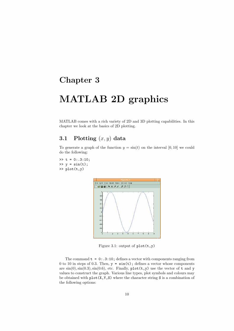
To generate a graph of the function y = sin(t) on the interval [0, 10] we coulddo the following:
>> t = 0:.3:10;
>> y = sin(t);
>> plot(t,y)
Figure 3.1: output of plot(t,y)
The command t = 0:.3:10; defines a vector with components ranging from0 to 10 in steps of 0.3. Then, y = sin(t); defines a vector whose componentsare sin(0), sin(0.3), sin(0.6), etc. Finally, plot(t,y) use the vector of t and y
values to construct the graph. Various line types, plot symbols and colours maybe obtained with plot(X,Y,S) where the character string S is a combination ofthe following options:
10
3.2. FUNCTION PLOTS 11
colour data points line type
r red . point - solidg green o circle -- dashedb blue x x-mark : dotted
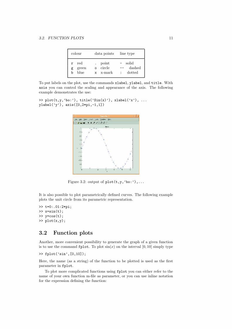
To put labels on the plot, use the commands xlabel, ylabel, and title. Withaxis you can control the scaling and appearance of the axis. The followingexample demonstrates the use:
>> plot(t,y,’bo:’), title(’Sin(x)’), xlabel(’x’), ...
ylabel(’y’), axis([0,2*pi,-1,1])
Figure 3.2: output of plot(t,y,’bo:’),...
It is also possible to plot parametrically defined curves. The following exampleplots the unit circle from its parametric representation.
>> t=0:.01:2*pi;
>> x=sin(t);
>> y=cos(t);
>> plot(x,y);
3.2 Function plots
Another, more convenient possibility to generate the graph of a given functionis to use the command fplot. To plot sin(x) on the interval [0, 10] simply type
>> fplot(’sin’,[0,10]);
Here, the name (as a string) of the function to be plotted is used as the firstparameter in fplot.
To plot more complicated functions using fplot you can either refer to thename of your own function m-file as parameter, or you can use inline notationfor the expression defining the function:

12 CHAPTER 3. MATLAB 2D GRAPHICS
>> fplot(’x*sin(x)’,[0,10]);
This plots the function y = x · sin(x) on the interval [0, 10]. x is just a place-holder in the above expression and has nothing to do with x as a variable.
Chapter 4
Programming
MATLAB includes a modern, interpreted programming language.
4.1 m-Files
Files that contain MATLAB source code are called m-files (extension .m ). Thereare two kinds of m-files: script files and function files.
• Script m-files do not process any arguments. Upon typing the name ofthe file (without the extension .m), the commands contained in the file areexecuted as if they had been entered at the keyboard.
• Function m-files contain a line with a function definition. These maytake input arguments and return output arguments. They can be calledin the same way as built-in functions.
4.2 Where to save m-Files
You create an m-file with the editor built in to MATLAB (File→New→M-
File) or your favourite editor (e.g. pico, emacs, vi). You can save the file in anydirectory you like. However, for MATLAB to find the file, the file either has tobe either in MATLAB’s working directory or in MATLAB’s search path.
To find out the working directory, use pwd:
>> pwd
ans =
/a/canonmills/disk/home/canonmills/sterratt
You can change the working directory using cd. For example if you store someM-files in /home/sterratt/my_mfiles, do
>> cd my_mfiles
>> pwd
ans =
13
14 CHAPTER 4. PROGRAMMING
/a/canonmills/disk/home/canonmills/sterratt
>>
Alternatively you and discover the directories in the MATLAB search path usingpath:
>> path
MATLABPATH
/opt/matlab-7.0.1/toolbox/matlab/general
/opt/matlab-7.0.1/toolbox/matlab/ops
/opt/matlab-7.0.1/toolbox/matlab/lang
...
You can add your directory to the path like this:
>> addpath /home/sterratt/my_mfiles -end
Now you can use any files in /home/sterratt/my mfiles whatever the MAT-LAB working directory.
4.3 My first MATLAB program
Here is an example of a small script m-file - let us save it under the namefirstprog.m:
% Script file firstprog.m
x = pi/100:pi/100:10*pi;
y = sin(x)./x;
plot(x,y)
grid
Let us analyse the contents of this file. The first line begins with the percentagesign %. This is a comment. All comments are ignored by MATLAB. They areadded to improve readability of the code. In the next two lines arrays x and y
are created. Note that the semicolon follows both commands. This suppressesdisplay of the content of both vectors to the screen. The array x holds 1000evenly spaced numbers in the interval [ π
100 , 10 π] while the array y holds the
values of the function y = sin(x)x
at these points. Recall that the dot operator .before the right division operator / specifies the component-wise division of thearrays sin(x) and x. The command plot creates the graph of the sin functionusing the points previously generated. Finally, the command grid is executed.This adds a grid to the graph. We invoke this file by typing its name in theCommand Window and next pressing Enter.
>> firstprog

4.4. CONTROL FLOW 15
Figure 4.1: output of firstprog
4.4 Control flow
To control the flow of commands you can use the following structures: for-loops,while-loops, if-else-end and switch-case. These can be used in interactivemode, but their main purpose is programming using m-files.
4.4.1 Repeating with for-loops
The syntax of the for-loop is shown below:
for k = array
commands
end
The commands between the for and end statements are executed for all valuesstored in the array. Note that the end statement is necessary in any case, evenif the body of the loop consists of a single command only.
As an example, suppose that we want to model a leaky integrating neuron.We could save the following in an m-file called integrator.m.
I0 = 1; % Input current in nA
dt = 1; % time step in ms
tau = 10; % membrane time constant in ms
nstep = 100; % Number of timesteps to integrate over
v(1) = 0; % Voltage in mV
Rin = 5; % Input resistance in MOhm
t = (1:nstep)*dt;
for n=2:nstep
v(n) = v(n-1) + dt*(- v(n-1)/tau + Rin*I0/tau);
end
plot(t,v)
Now run the file by typing integrator.
16 CHAPTER 4. PROGRAMMING
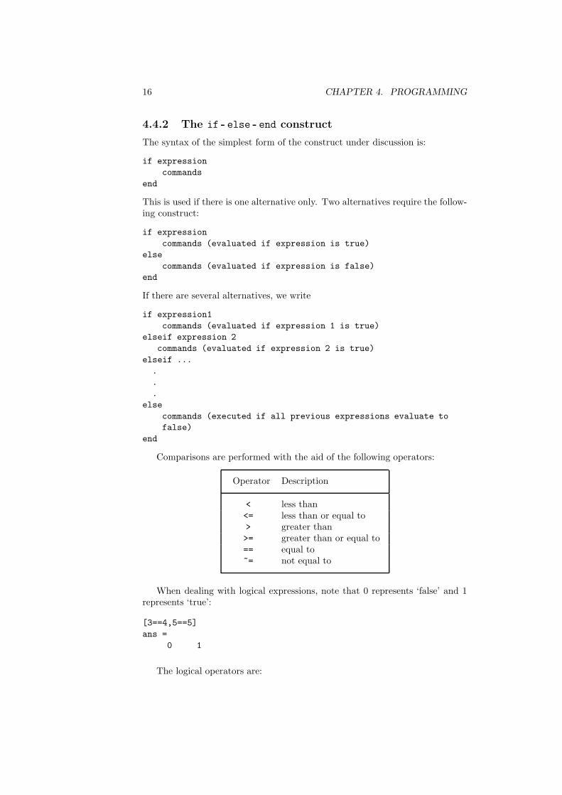
4.4.2 The if - else - end construct
The syntax of the simplest form of the construct under discussion is:
if expression
commands
end
This is used if there is one alternative only. Two alternatives require the follow-ing construct:
if expression
commands (evaluated if expression is true)
else
commands (evaluated if expression is false)
end
If there are several alternatives, we write
if expression1
commands (evaluated if expression 1 is true)
elseif expression 2
commands (evaluated if expression 2 is true)
elseif ...
.
.
.
else
commands (executed if all previous expressions evaluate to
false)
end
Comparisons are performed with the aid of the following operators:
Operator Description
< less than<= less than or equal to> greater than>= greater than or equal to== equal to~= not equal to
When dealing with logical expressions, note that 0 represents ‘false’ and 1represents ‘true’:
[3==4,5==5]
ans =
0 1
The logical operators are:
4.4. CONTROL FLOW 17
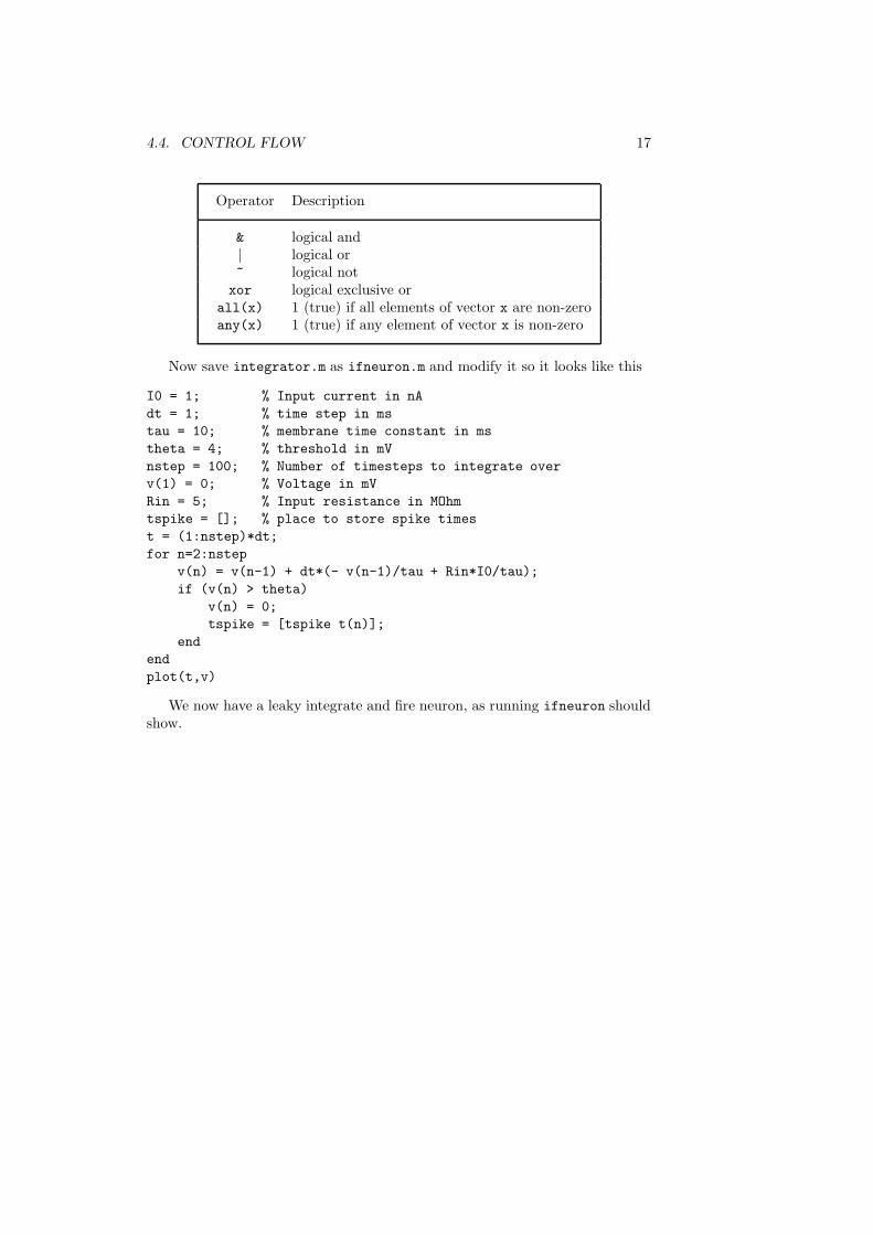
Operator Description
& logical and| logical or~ logical notxor logical exclusive or
all(x) 1 (true) if all elements of vector x are non-zeroany(x) 1 (true) if any element of vector x is non-zero
Now save integrator.m as ifneuron.m and modify it so it looks like this
I0 = 1; % Input current in nA
dt = 1; % time step in ms
tau = 10; % membrane time constant in ms
theta = 4; % threshold in mV
nstep = 100; % Number of timesteps to integrate over
v(1) = 0; % Voltage in mV
Rin = 5; % Input resistance in MOhm
tspike = []; % place to store spike times
t = (1:nstep)*dt;
for n=2:nstep
v(n) = v(n-1) + dt*(- v(n-1)/tau + Rin*I0/tau);
if (v(n) > theta)
v(n) = 0;
tspike = [tspike t(n)];
end
end
plot(t,v)
We now have a leaky integrate and fire neuron, as running ifneuron shouldshow.

Chapter 5
MATLAB Matrices, and
other data types
As in the case of scalar variables, arrays need not to be declared, and MATLABperforms automatic storage allocation. In the following we describe the basictechniques for creating and operating with 1-dimensional arrays (vectors) and2-dimensional arrays (matrices).
5.1 Dense vectors and matrices
This command creates a row vector:
>> a = [1 2 3]
a =
1 2 3
Column vectors are specified in a similar way. However, semicolons must sepa-rate the components of a column vector:
>> b = [1;2;3]
b =
1
2
3
Alternatively, the components of a column vector may be entered on separatelines (by pressing Enter instead of typing ;).
The quote operator ’ is used to create the transpose of a vector (matrix)1:
>> a’
ans =
1Strictly speaking, ’ creates the conjugate transpose, but this is only relevant if we aredealing with numbers with imaginary parts. The dot-quote operator .’ creates the truetranspose vector (matrix).
18
5.1. DENSE VECTORS AND MATRICES 19
1
2
3
The command length returns the number of components of a vector:
>> length(a)
ans =
3
This creates a 3-by-3 matrix:
>> A = [1 2 3;4 5 6;7 8 10]
A =
1 2 3
4 5 6
7 8 10
Note that the semicolon operator ; separates the rows. To extract a singleelement of an array, use round braces:
>> A(3,2)
ans =
8
The colon : stands for a full range of indices. It can e.g. be used to extract awhole row or column of an array:
>> A(2,:)
ans =
4 5 6
>> A(:,3)
ans =
3
6
10
A submatrix B consisting of rows 1 and 3 and columns 1 and 2 of the matrix A
is achieved in the following way:
>> B = A([1 3], [1 2])
B =
1 2
7 8
To interchange rows 1 and 3 of A use the vector of row indices together with thecolon operator:
>> C = A([3 2 1],:)
C =
7 8 10
4 5 6
1 2 3
20 CHAPTER 5. MATLAB MATRICES, AND OTHER DATA TYPES
To delete a row (column) use the empty vector []:
>> A(:, 2) = []
A =
1 3
4 6
7 10
The second column of A is now deleted. To insert a row (column) we use thetechnique for creating matrices and vectors:
>> A = [A(:,1) [2 5 8]’ A(:,2)]
A =
1 2 3
4 5 6
7 8 10
The matrix A has now been restored to its original form.
5.2 Special matrix functions
The function diag creates a diagonal matrix with diagonal entries taken froma given vector:
>> d = [1 2 3];
>> D = diag(d)
D =
1 0 0
0 2 0
0 0 3
To extract the main diagonal of the matrix D we use the function diag again:
>> d = diag(D)
d =
1
2
3
The function inv is used to compute the inverse of a matrix. Let, for in-stance, the matrix A be defined as follows:
>> A = [1 2 3;4 5 6;7 8 10]
A =
1 2 3
4 5 6
7 8 10
Then,
5.3. CELL AND STRUCTURE ARRAYS 21
>> B = inv(A)
B =
-0.6667 -1.3333 1.0000
-0.6667 3.6667 -2.0000
1.0000 -2.0000 1.0000
The command find can be used for finding the indices of the nonzero entriesof a vector or a matrix and is often used with sparse matrices.find(x) returns an array containing the indices of the nonzero elements of thevector x. [i,j]=find(A) returns the row and column indices of the nonzeroelements of the (sparse) matrix A. [i,j,v]=find(A) also returns the row andcolumn indices of nonzero elements of A and as third output parameter it returnsa vector containing the values of the nonzero elements.For example we could find the value of the absolute smallest nonzero elementof a given matrix A like this:
>> [i,j,v]=find(A);
>> minimum=min(abs(v));
It is often useful to start with a predefined matrix providing only the dimen-sion. A partial list of these functions is:
zeros matrix filled with 0ones matrix filled with 1eye Identity matrixrand matrix with uniformly distributed random numbers
For example
>> zeros(1,5)
ans =
0 0 0 0 0
>> rand(2,3)
ans =
0.9501 0.6068 0.8913
0.2311 0.4860 0.7621
5.3 Cell and structure arrays
Cell arrays are arrays which contain elements of arbitrary types. They areidentified by curly braces instead of square ones:
>> c = {[3,4],18.2,[1,2;2,1],’string’};
defines a cell array c. We can access elements of c in the following way:
22 CHAPTER 5. MATLAB MATRICES, AND OTHER DATA TYPES
>> c{3}
ans =
1 2
2 1
A structure array is an array consisting of several variables where each hasits own type and identifier.
>> p.pol=’x^2-3*x+2’;p.coef=[1,-3,2];p.zeros=[1,2];p.min=[-1/4]
p =
pol: ’x^2-3*x+2’
coef: [1 -3 2]
zeros: [1 2]
min: -0.2500
defines a structure array p. The elements of a structure array are accessed byarray.identifier, e.g.:
>> p.zeros
ans =
1 2
Chapter 6
More programming
In this chapter we will use some of the useful predefined matrices we met inthe last chapter to make the integrate-and-fire neuron more efficient and noisy.We’ll then learn how to write functions and write one to compute the interspikeinterval histogram. We’ll round off with a brief introduction to input and outputto screen and files.
6.1 Making code efficient
Run the ifneuron m-file like this:
>> clear v; starttime = cputime; ifneuron; cputime - starttime
ans =
0.1100
This first of all clears the contents of the v vector from memory. The cputime
command returns the current CPU time. This is first recorded in the variablestarttime, the ifneuron m-file is then run, and afterwards the difference (inseconds)between the time at the start and the time at the end is printed out inans.
Change the value of nstep in the ifneuron m-file to 10000, 20000, 30000and 40000 running the ifneuron script each time. Is the increase in time takena linear function of the number of time steps?
The reason for the poor performance is that when we set an element of thevector v that doesn’t yet exist (in the for loop), MATLAB makes space for anew vector with size n+1 in memory. The time taken to allocate memory spaceis proportional to size, so the total time taken in the program will be aboutn(n−1)
2 .We can improve performance dramatically by allocating all the space before
we enter the for loop. To do this, replace the line
v(1) = 0; % Voltage in mV
with
23
24 CHAPTER 6. MORE PROGRAMMING
v = zeros(1,nstep); % Allocate space for voltage in mV
This fills the vector v with nstep zeros, so no allocation has to take place inthe for loop. Try timing the modified m-file to prove this!
6.2 Adding some noise
Suppose we want to see what happens if the current we inject is a bit noisy. Trysaving ifneuron.m as noisyifneuron.m and modifying it so that it reads
nstep = 100; % Number of timesteps to integrate over
Inoise = 0.1;
I0 = 1+Inoise*randn(1,nstep); % Input current in nA
dt = 1; % time step in ms
tau = 10; % membrane time constant in ms
theta = 4; % threshold in mV
v = zeros(1,nstep);
Rin = 5; % Input resistance in MOhm
tspike = [];
t = (1:nstep)*dt;
for n=2:nstep
v(n) = v(n-1) + dt*(- v(n-1)/tau + Rin*I0(n)/tau);
if (v(n) > theta)
v(n) = 0;
tspike = [ tspike t(n) ];
end
end
plot(t,v)
We have used randn to generate a noisy input current with Gaussian whitenoise. Try changing Inoise to change how noisy the neuron is.
6.3 My first MATLAB function
Here is an example of a function m-file called isi.m
function isi_result=isi(spiketimes)
% ISI produces interspike intervals from spike times
% ISI(spiketimes) returns the interspike intervals
% of SPIKETIMES
if (length(spiketimes)>1)
isi_result = diff(spiketimes);
else
isi_result = [];
end
Note the difference between the function name isi and the result variable,or output argument, isi result. The function name must coincide with thename of the m-file in which the function is stored.
The function can be then called in the same way as a predefined function,e.g.
6.4. INPUT, OUTPUT, AND FILE HANDLING 25
>> isi(tspike)
ans =
18 16 16 16 16
The isi function returns the interspike intervals of a spike train represented byspike times. We can plot this using the hist command:
>> hist(isi(tspike),1:100); xlabel(’ISI /ms’); ylabel(’counts’);
The second argument sets the bin centres.
6.4 Input, output, and file handling
The disp command can be used to display expressions or contents of variablesto the screen during the execution of functions or script files:
disp(’string expression’);
string expression
A=[3,2;2,3];
disp(A);
3 2
2 3
The input function can be used for requesting user input. For example,
r=input(’value for r: ’);
displays value for r: to the screen and waits for the user to enter an ex-pression which is then assigned to r.
To display formatted output to the screen you can use the function fprintf,with a syntax similar as in C:
fprintf (’approximation for pi: %6.4f\n’,pi)
approximation for pi: 3.1416
For further variants of formatting consult the online help.
It is also possible to read and write data to and from files. Here is an exampleof how we might save the spike time data to file:
>> f = fopen(’spikedata.txt’,’w’)
f =
3
>> fprintf(f,’%g ’,tspike)

26 CHAPTER 6. MORE PROGRAMMING
ans =
18
>> fclose(f)
ans =
0
Here we give a short description of some of the most important MATLABfile handling functions. For more details please refer to MATLAB’s help facility.
• ID=fopen(name,permission) opens the file specified by name with thespecified permission (’r’..read, ’w’..write, ’a’..append, ...) anda value is stored to ID with which the file can be accessed later.
• fclose(ID) closes the file specified by ID.
• fprintf(ID,format,A,...) writes formatted data to the file specifiedby ID. format is a string containing C conversion specifications. If noparameter ID is passed, fprintf writes to the screen.
• [A,count]=fscanf(ID,format,size) reads formatted data from the filespecified by ID. format is a string containing C conversion specifications.The size parameter puts a limit on the number of elements to be readfrom the file (optional). The data read from the file are stored to A. Ifthe optional output parameter count is used, it is assigned the number ofelements successfully read.
Chapter 7
MATLAB arithmetic
operators
7.1 Computing with vectors and matrices
We now explain how to perform arithmetic operations with vectors and matrices– the main strength of MATLAB. The matrix/vector - arithmetic operations areaddition (+), subtraction (-) and multiplication (*). Addition and subtractionare only defined if the matrices have the same dimensions. Multiplication onlyworks if the matrices have equal inner dimensions: I.e., if A is an n×m matrixand B is an p×q matrix, then A*B is well-defined (and is calculated by MATLAB)if m = p. MATLAB also allows for powers (^) of square matrices.
Continuing with matrix operations:
>> A = [1 2 3;4 5 6];
>> A*A
??? Error using ==> * Inner matrix dimensions must agree.
>> A*A’
ans =
14 32
32 77
The \ operator solves linear systems of equations. If you desire the solutionof A x=b, then the most simple method using MATLAB to find x is to set x =
A\b. If A is an n×m matrix and B is an p×q matrix then A\b is defined (andis calculated by MATLAB) if m = p. For non-square and singular systems, theoperation A\b gives the solution in the least squares sense.
Example: Let
>> A = [1 2 3;4 5 6;7 8 10]
A =
1 2 3
4 5 6
7 8 10
and let
27
28 CHAPTER 7. MATLAB ARITHMETIC OPERATORS
>> b = ones(3,1);
Then,
>> x = A\b
x =
-1.0000
1.0000
0.0000
In order to verify correctness of the computed solution, let us compute theresidual vector r:
>> r = b - A*x
r =
1.0e-015 *
0.1110
0.6661
0.2220
Theoretically, the entries of the computed residual r should all be equal tozero. This example illustrates an effect of the roundoff errors on the computedsolution.
If m > n, then the system A x=b is overdetermined and in most cases thesystem is inconsistent. A special solution to the system A x=b, again obtainedwith the aid of the backslash operator \ , is the least-squares solution. Let
>> A = [2 1; 1 10; 1 2];
and let the vector of the right-hand sides be the same as the one in the precedingexample. Then,
>> x = A\b
x =
0.5484
0.0507
The residual of the computed solution is:
>> r = b - A*x
r =
-0.1475
-0.0553
0.3502