An Introduction to Nonlinear Dimensionality Reductionby Maximum Variance Unfolding

Kilian Q. Weinberger and Lawrence K. SaulDepartment of Computer and Information Science, University of Pennsylvania

Levine Hall, 3330 Walnut Street, Philadelphia, PA 19104-6389{kilianw,lsaul}@cis.upenn.edu

Abstract

Many problems in AI are simplified by clever representationsof sensory or symbolic input. How to discover such rep-resentations automatically, from large amounts of unlabeleddata, remains a fundamental challenge. The goal of statis-tical methods for dimensionality reduction is to detect anddiscover low dimensional structure in high dimensional data.In this paper, we review a recently proposed algorithm—maximum variance unfolding—for learning faithful low di-mensional representations of high dimensional data. Thealgorithm relies on modern tools in convex optimizationthat are proving increasingly useful in many areas of ma-chine learning.

IntroductionA fundamental challenge of AI is to develop useful internalrepresentations of the external world. The human brain ex-cels at extracting small numbers of relevant features fromlarge amounts of sensory data. Consider, for example, howwe perceive a familiar face. A friendly smile or a menac-ing glare can be discerned in an instant and described bya few well chosen words. On the other hand, the digitalrepresentations of these images may consist of hundreds orthousands of pixels. Clearly, there are much more compactrepresentations of images, sounds, and text than their nativedigital formats. With such representations in mind, we havespent the last few years studying the problem of dimension-ality reduction—how to detect and discover low dimensionalstructure in high dimensional data.

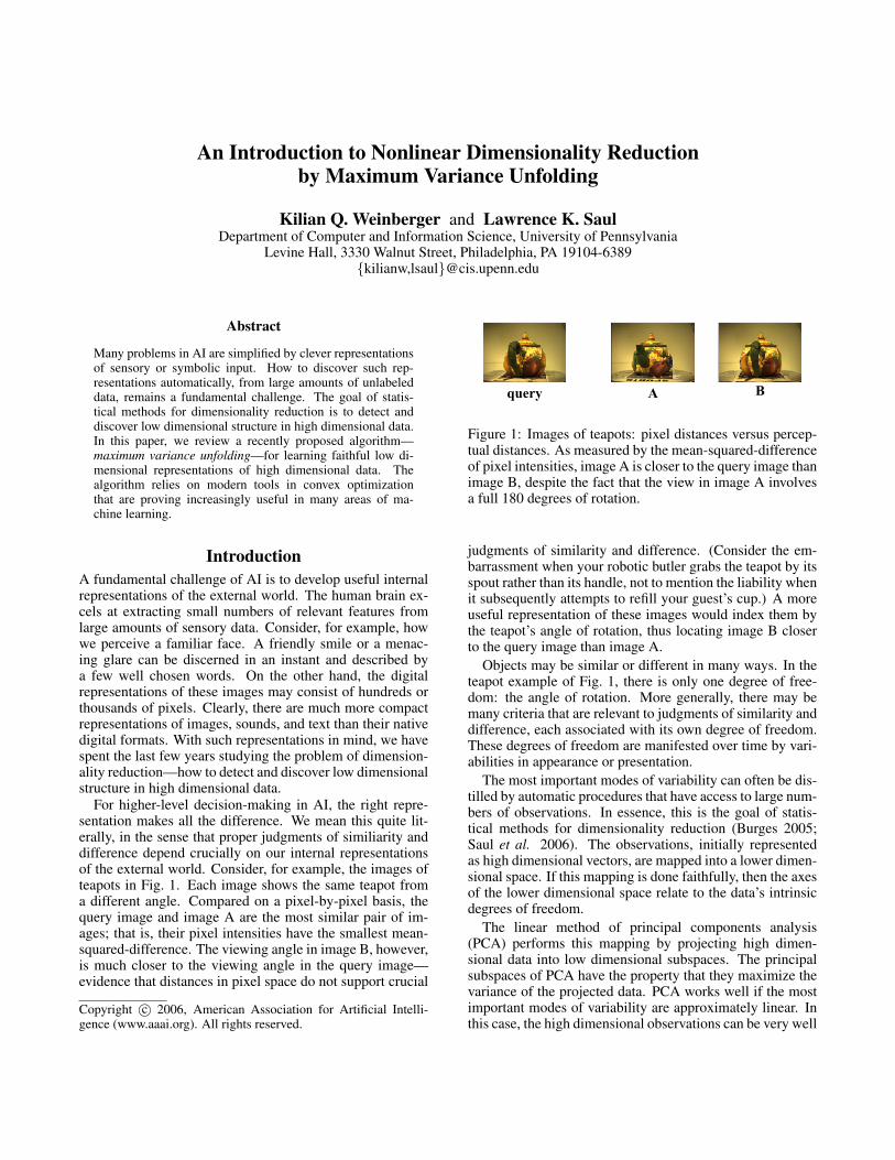
For higher-level decision-making in AI, the right repre-sentation makes all the difference. We mean this quite lit-erally, in the sense that proper judgments of similiarity anddifference depend crucially on our internal representationsof the external world. Consider, for example, the images ofteapots in Fig. 1. Each image shows the same teapot froma different angle. Compared on a pixel-by-pixel basis, thequery image and image A are the most similar pair of im-ages; that is, their pixel intensities have the smallest mean-squared-difference. The viewing angle in image B, however,is much closer to the viewing angle in the query image—evidence that distances in pixel space do not support crucial

Copyright c© 2006, American Association for Artificial Intelli-gence (www.aaai.org). All rights reserved.

query A B

Figure 1: Images of teapots: pixel distances versus percep-tual distances. As measured by the mean-squared-differenceof pixel intensities, image A is closer to the query image thanimage B, despite the fact that the view in image A involvesa full 180 degrees of rotation.

judgments of similarity and difference. (Consider the em-barrassment when your robotic butler grabs the teapot by itsspout rather than its handle, not to mention the liability whenit subsequently attempts to refill your guest’s cup.) A moreuseful representation of these images would index them bythe teapot’s angle of rotation, thus locating image B closerto the query image than image A.

Objects may be similar or different in many ways. In theteapot example of Fig. 1, there is only one degree of free-dom: the angle of rotation. More generally, there may bemany criteria that are relevant to judgments of similarity anddifference, each associated with its own degree of freedom.These degrees of freedom are manifested over time by vari-abilities in appearance or presentation.

The most important modes of variability can often be dis-tilled by automatic procedures that have access to large num-bers of observations. In essence, this is the goal of statis-tical methods for dimensionality reduction (Burges 2005;Saul et al. 2006). The observations, initially representedas high dimensional vectors, are mapped into a lower dimen-sional space. If this mapping is done faithfully, then the axesof the lower dimensional space relate to the data’s intrinsicdegrees of freedom.

The linear method of principal components analysis(PCA) performs this mapping by projecting high dimen-sional data into low dimensional subspaces. The principalsubspaces of PCA have the property that they maximize thevariance of the projected data. PCA works well if the mostimportant modes of variability are approximately linear. Inthis case, the high dimensional observations can be very well

original

8 16 32 64 560

reconstructions2 4 8 16 32 64 128 256 512Original 0 0.5 12 4 8 16 32 64 128 256 512Original 0 0.5 1

4

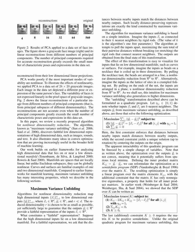
Figure 2: Results of PCA applied to a data set of face im-ages. The figure shows a grayscale face image (right) and itslinear reconstructions from different numbers of principalcomponents. The number of principal components requiredfor accurate reconstruction greatly exceeds the small num-ber of characteristic poses and expressions in the data set.

reconstructed from their low dimensional linear projections.PCA works poorly if the most important modes of vari-

ability are nonlinear. To illustrate the effects of nonlinearity,we applied PCA to a data set of 28 × 20 grayscale images.Each image in the data set depicted a different pose or ex-pression of the same person’s face. The variability of faces isnot expressed linearly in the pixel space of grayscale images.Fig. 2 shows the linear reconstructions of a particular im-age from different numbers of principal components (that is,from principal subspaces of different dimensionality). Thereconstructions are not accurate even when the number ofprincipal components greatly exceeds the small number ofcharacteristic poses and expressions in this data set.

In this paper, we review a recently proposed algorithmfor nonlinear dimensionality reduction. The algorithm,known as “maximum variance unfolding” (Sun et al. 2006;Saul et al. 2006), discovers faithful low dimensional repre-sentations of high dimensional data, such as images, sounds,and text. It also illustrates many ideas in convex optimiza-tion that are proving increasingly useful in the broader fieldof machine learning.

Our work builds on earlier frameworks for analyzinghigh dimensional data that lies on or near a low dimen-sional manifold (Tenenbaum, de Silva, & Langford 2000;Roweis & Saul 2000). Manifolds are spaces that are locallylinear, but unlike Euclidean subspaces, they can be globallynonlinear. Curves and surfaces are familiar examples of oneand two dimensional manifolds. Compared to earlier frame-works for manifold learning, maximum variance unfoldinghas many interesting properties, which we describe in thefollowing sections.

Maximum Variance UnfoldingAlgorithms for nonlinear dimensionality reduction maphigh dimensional inputs {~xi}n

i=1 to low dimensional out-puts {~yi}n

i=1, where ~xi ∈ <d, ~yi ∈ <r, and r � d. The re-duced dimensionality r is chosen to be as small as possible,yet sufficiently large to guarantee that the outputs ~yi ∈ <r

provide a faithful representation of the inputs ~xi ∈ <d.What constitutes a “faithful” representation? Suppose

that the high dimensional inputs lie on a low dimensionalmanifold. For a faithful representation, we ask that the dis-

tances between nearby inputs match the distances betweennearby outputs. Such locally distance-preserving represen-tations are exactly the kind constructed by maximum vari-ance unfolding.

The algorithm for maximum variance unfolding is basedon a simple intuition. Imagine the inputs ~xi as connectedto their k nearest neighbors by rigid rods. (The value of kis the algorithm’s one free parameter.) The algorithm at-tempts to pull the inputs apart, maximizing the sum total oftheir pairwise distances without breaking (or stretching) therigid rods that connect nearest neighbors. The outputs areobtained from the final state of this transformation.

The effect of this transformation is easy to visualize forinputs that lie on low dimensional manifolds, such as curvesor surfaces. For example, imagine the inputs as beads on anecklace that is coiled up in three dimensions. By pullingthe necklace taut, the beads are arranged in a line, a nonlin-ear dimensionality reduction from <3 to <1. Alternatively,imagine the inputs as the lattice of sites in a crumpled fish-ing net. By pulling on the ends of the net, the inputs arearranged in a plane, a nonlinear dimensionality reductionfrom <3 to <2. As we shall see, this intuition for maximumvariance unfolding also generalizes to higher dimensions.

The “unfolding” transformation described above can beformulated as a quadratic program. Let ηij ∈ {0, 1} de-note whether inputs ~xi and ~xj are k-nearest neighbors. Theoutputs ~yi from maximum variance unfolding, as describedabove, are those that solve the following optimization:

Maximize∑

ij ‖~yi − ~yj‖2 subject to:(1) ‖~yi − ~yj‖2 = ‖~xi − ~xj‖2 for all (i, j) with ηij =1.(2)

∑i ~yi = 0

Here, the first constraint enforces that distances betweennearby inputs match distances between nearby outputs,while the second constraint yields a unique solution (up torotation) by centering the outputs on the origin.

The apparent intractability of this quadratic program canbe finessed by a simple change of variables. Note thatas written above, the optimization over the outputs ~yi isnot convex, meaning that it potentially suffers from spu-rious local minima. Defining the inner product matrixKij = ~yi · ~yj , we can reformulate the optimization as asemidefinite program (SDP) (Vandenberghe & Boyd 1996)over the matrix K. The resulting optimization is simplya linear program over the matrix elements Kij , with theadditional constraint that the matrix K has only nonnega-tive eigenvalues, a property that holds for all inner prod-uct matrices. In earlier work (Weinberger & Saul 2004;Weinberger, Sha, & Saul 2004), we showed that the SDPover K can be written as:Maximize trace(K) subject to:

(1) Kii−2Kij +Kjj = ‖~xi−~xj‖2 for all (i, j)with ηij =1.

(2) ΣijKij = 0.(3) K � 0.

The last (additional) constraint K � 0 requires the ma-trix K to be positive semidefinite. Unlike the originalquadratic program for maximum variance unfolding, this

SDP is convex. In particular, it can be solved efficiently withpolynomial-time guarantees, and many off-the-shelf solversare available in the public domain.

From the solution of the SDP in the matrix K, we canderive outputs ~yi ∈ <n satisfying Kij = ~yi · ~yj by singu-lar value decomposition. An r-dimensional representationthat approximately satisfies Kij ≈ ~yi · ~yj can be obtainedfrom the top r eigenvalues and eigenvectors of K. Roughlyspeaking, the number of dominant eigenvalues of K indi-cates the number of dimensions needed to preserve localdistances while maximizing variance. In particular, if thetop r eigenvalues of K account for (say) 95% of its trace,this indicates that an r-dimensional representation can cap-ture 95% of the unfolded data’s variance.

Experimental ResultsWe have used maximum variance unfolding (MVU) to ana-lyze many high dimensional data sets of interest. Here weshow some solutions (Weinberger & Saul 2004; Blitzer et al.2005) that are particularly easy to visualize.

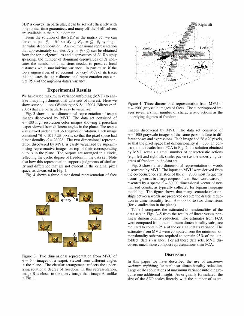
Fig. 3 shows a two dimensional representation of teapotimages discovered by MVU. The data set consisted ofn=400 high resolution color images showing a porcelainteapot viewed from different angles in the plane. The teapotwas viewed under a full 360 degrees of rotation. Each imagecontained 76 × 101 RGB pixels, so that the pixel space haddimensionality d = 23028. The two dimensional represen-tation discovered by MVU is easily visualized by superim-posing represenative images on top of their correspondingoutputs in the plane. The outputs are arranged in a circle,reflecting the cyclic degree of freedom in the data set. Notealso how this representation supports judgments of similar-ity and difference that are not evident in the original pixelspace, as discussed in Fig. 1.

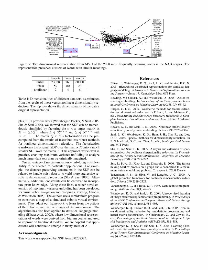
Fig. 4 shows a three dimensional representation of face

B

A

query

Figure 3: Two dimensional representation from MVU ofn = 400 images of a teapot, viewed from different anglesin the plane. The circular arrangement reflects the under-lying rotational degree of freedom. In this representation,image B is closer to the query image than image A, unlikein Fig. 1.

Right tilt

Left tilt

Pucker

Smile

Figure 4: Three dimensional representation from MVU ofn=1960 grayscale images of faces. The superimposed im-ages reveal a small number of characteristic actions as theunderlying degrees of freedom.

images discovered by MVU. The data set consisted ofn=1960 grayscale images of the same person’s face in dif-ferent poses and expressions. Each image had 28×20 pixels,so that the pixel space had dimensionality d = 560. In con-trast to the results from PCA in Fig. 2, the solution obtainedby MVU reveals a small number of characteristic actions(e.g., left and right tilt, smile, pucker) as the underlying de-grees of freedom in the data set.

Fig. 5 shows a two dimensional representation of wordsdiscovered by MVU. The inputs to MVU were derived fromthe co-occurrence statistics of the n=2000 most frequentlyoccuring words in a large corpus of text. Each word was rep-resented by a sparse d = 60000 dimensional vector of nor-malized counts, as typically collected for bigram languagemodeling. The figure shows that many semantic relation-ships between words are preserved despite the drastic reduc-tion in dimensionality from d = 60000 to two dimensions(for visualization in the plane).

Table 1 compares the estimated dimensionalities of thedata sets in Figs. 3–5 from the results of linear versus non-linear dimensionality reduction. The estimates from PCAwere computed from the minimum dimensionality subspacerequired to contain 95% of the original data’s variance. Theestimates from MVU were computed from the minimum di-mensionality subspace required to contain 95% of the “un-folded” data’s variance. For all these data sets, MVU dis-covers much more compact representations than PCA.

DiscussionIn this paper we have described the use of maximumvariance unfolding for nonlinear dimensionality reduction.Large-scale applications of maximum variance unfolding re-quire one additional insight. As originally formulated, thesize of the SDP scales linearly with the number of exam-

MAY, WOULD, COULD, SHOULD,

MIGHT, MUST, CAN, CANNOT,

COULDN'T, WON'T, WILL

ONE, TWO, THREE,

FOUR, FIVE, SIX,

SEVEN, EIGHT, NINE,

TEN, ELEVEN,

TWELVE, THIRTEEN,

FOURTEEN, FIFTEEN,

SIXTEEN,

SEVENTEEN,

EIGHTEEN

JANUARY

FEBRUARY

MARCH

APRIL

JUNE

JULY

AUGUST

SEPTEMBER

OCTOBER

NOVEMBER

DECEMBER

MILLION

BILLION

MONDAY

TUESDAY

WEDNESDAY

THURSDAY

FRIDAY

SATURDAY

SUNDAY

ZERO

Figure 5: Two dimensional representation from MVU of the 2000 most frequently occuring words in the NAB corpus. Therepresentation preserves clusters of words with similar meanings.

teapots faces wordsinitial 23028 560 60000linear 59 80 23

nonlinear 2 4 6

Table 1: Dimensionalities of different data sets, as estimatedfrom the results of linear versus nonlinear dimensionality re-duction. The top row shows the dimensionality of the data’soriginal representation.

ples, n. In previous work (Weinberger, Packer, & Saul 2005;Sha & Saul 2005), we showed that the SDP can be tremen-dously simplified by factoring the n × n target matrix asK ≈ QLQ>, where L ∈ Rm×m and Q ∈ Rn×m withm � n. The matrix Q in this factorization can be pre-computed from the results of faster but less robust methodsfor nonlinear dimensionality reduction. The factorizationtransforms the original SDP over the matrix K into a muchsmaller SDP over the matrix L. This approach works well inpractice, enabling maximum variance unfolding to analyzemuch larger data sets than we originally imagined.

One advantage of maximum variance unfolding is its flex-ibility to be adapted to particular applications. For exam-ple, the distance-preserving constraints in the SDP can berelaxed to handle noisy data or to yield more aggressive re-sults in dimensionality reduction (Sha & Saul 2005). Alter-natively, additional constraints can be enforced to incorpo-rate prior knowledge. Along these lines, a rather novel ex-tension of maximum variance unfolding has been developedfor visual robot navigation and mapping (Bowling, Ghodsi,& Wilkinson 2005). The authors use a semidefinite programto construct a map of a simulated robot’s virtual environ-ment. They adapt our framework to learn from the actionsof the robot as well as the images of its environment. Thealgorithm has also been applied to statistical language mod-eling (Blitzer et al. 2005), where low dimensional represen-tations of words were derived from bigram counts and usedto improve on traditional models. We are hopeful that appli-cations will continue to emerge in many areas of AI.

AcknowledgmentsThis work was supported by NSF Award 0238323.

ReferencesBlitzer, J.; Weinberger, K. Q.; Saul, L. K.; and Pereira, F. C. N.2005. Hierarchical distributed representations for statistical lan-guage modeling. In Advances in Neural and Information Process-ing Systems, volume 17. Cambridge, MA: MIT Press.Bowling, M.; Ghodsi, A.; and Wilkinson, D. 2005. Action re-specting embedding. In Proceedings of the Twenty-second Inter-national Conference on Machine Learning (ICML-05), 65–72.Burges, C. J. C. 2005. Geometric methods for feature extrac-tion and dimensional reduction. In Rokach, L., and Maimon, O.,eds., Data Mining and Knowledge Discovery Handbook: A Com-plete Guide for Practitioners and Researchers. Kluwer AcademicPublishers.Roweis, S. T., and Saul, L. K. 2000. Nonlinear dimensionalityreduction by locally linear embedding. Science 290:2323–2326.Saul, L. K.; Weinberger, K. Q.; Ham, J. H.; Sha, F.; and Lee,D. D. 2006. Spectral methods for dimensionality reduction. InB. Schoelkopf, O. C., and Zien, A., eds., Semisupervised Learn-ing. MIT Press.Sha, F., and Saul, L. K. 2005. Analysis and extension of spec-tral methods for nonlinear dimensionality reduction. In Proceed-ings of the Twenty-second International Conference on MachineLearning (ICML-05), 785–792.Sun, J.; Boyd, S.; Xiao, L.; and Diaconis, P. 2006. The fastestmixing Markov process on a graph and a connection to a maxi-mum variance unfolding problem. To appear in SIAM Review.Tenenbaum, J. B.; de Silva, V.; and Langford, J. C. 2000. Aglobal geometric framework for nonlinear dimensionality reduc-tion. Science 290:2319–2323.Vandenberghe, L., and Boyd, S. P. 1996. Semidefinite program-ming. SIAM Review 38(1):49–95.Weinberger, K. Q., and Saul, L. K. 2004. Unsupervised learningof image manifolds by semidefinite programming. In Proceedingsof the IEEE Conference on Computer Vision and Pattern Recog-nition (CVPR-04), volume 2, 988–995.Weinberger, K. Q.; Packer, B. D.; and Saul, L. K. 2005. Nonlin-ear dimensionality reduction by semidefinite programming andkernel matrix factorization. In Ghahramani, Z., and Cowell, R.,eds., Proceedings of the Tenth International Workshop on Artifi-cial Intelligence and Statistics (AISTATS-05), 381–388.Weinberger, K. Q.; Sha, F.; and Saul, L. K. 2004. Learning a ker-nel matrix for nonlinear dimensionality reduction. In Proceedingsof the Twenty First International Conference on Machine Learn-ing (ICML-04), 839–846.