an introduction to octave -...

An Introduction to Octave

for High School and University Students

Second Edition

Roger Herz-Fischler

Mzinhigan Publishing

An Introduction to Octave for High School and University Students

Second Edition

Copyright c© Roger Herz-Fischler 2016

Permission is given to redistribute and modify this work on a strictly non-commercial basis.Educational institutions and student organizations may distribute the whole text or parts of thetext on a cost plus basis.

Published 2016 by

Mzinhigan Publishing

340 Second Avenue, Ottawa, Ontario, Canada, K1S 2J2

e-mail: [email protected]

web site: http://web.ncf.ca/en493

“Mzinhigan” is the word for “book” in the Odawa (Ottawa) dialect of Ojibwa. The logo is“Mzinhigan” written in the related Algonquin language of Cree—as spoken on the west coastof James Bay—using Cree syllabics.

Library and Archives Canada Cataloguing in Publication

ISBN 978-0-9693002-9-8

Due to drastic cutbacks at Library and Archives Canada, the classification information was notavailable at the time of printing.

The following appears at the startup of Octave:

GNU Octave, version 3.6.4Copyright c© 2013 John W. Eaton and others.“This is free software; see the source code for copying conditions. There is ABSOLUTELYNO WARRANTY; not even for MERCHANTABILITY or FITNESS FOR A PARTICULARPURPOSE. For details, type ‘warranty’. ”

Additional information about Octave is available at http://www.octave.org

Matlab is a trademark of The Mathworks, Inc.

Preface

While teaching engineering, computer science and mathematics courses at the univer-sity level, I wrote A Guide to Matlab for the use of my students. In the period since my

retirement all the serious Linux distributions1 have included Octave, which is open-source and therefore free. These Linux distributions, which are also free, are now all“live” (i.e. they can be run directly from a DVD), available on the web and easy toinstall, even allowing for a dual boot on a Windows machine.

Octave and Matlab are what I would call “application languages” in the sense thatthey are both oriented towards applications involving mathematics. They are ideallysuited for working with arrays of numbers and because of this many mathematical andlogical situations can be programmed in a very concise manner. What other languages

can only do via “loops”—a feature which is of course also incorporated in Octave andMatlab—can often be evaluated by a short one-line statement which corresponds towhat one would write mathematically. So instead of just writing programs, one alsothinks mathematically. This feature alone makes them relatively easy to learn and ideal

for high-school and university students.

It was with all this in mind that I decided to write an introduction to Octave that wouldbe more suitable for students in the upper grades of high shool and for those beginninguniversity. I have limited the topics to those that I think will prove most useful and

have limited the number of new topics in each section. Each section—except for theintroductory section 01 and the intrinsically long section 07 on graphing—is only twopages long with each section dealing with just one topic.

Both Octave and Matlab are widely used in engineering and science in universitiesas well as in professional settings. They have many built-in, easy to use functions,which can be applied to a variety of situations, some of which will be illustrated inthis introduction. Octave commands have been made compatible with those of Matlabso that students who will be using Matlab later in their studies can make the transition

without any additional steps in the learning process. At a very advanced level, thereare packages in one which do not appear in the other, but this is not of concern to us atthe introductory level.

More advanced notions are described in my A Guide to Octave and Matlab. The latter,as well as revised versions of this Introduction to Octave are available—and may befreely distributed—on my web site:

http: //web.ncf.ca /en493

The web site also has the iso file for Student Linux which is pre-configured and in-

cludes Octave and other software,.

I may be contacted at:

student [email protected]

1. Octave is also available for Windows, Apple etc, See:

http: //www.gnu.org /software/octave/download.htm

Table of Contents

A ⋆, here and in the text, indicates a special topic. As indicated by the double star,section 18 involves a more complicated situation.

Section 01: A sample Octave session

Section 02: Common functions

Section 03: Defining your own functions

Section 04: Vectors – basic concepts

Section 05: Functions of vectors; data analysis; statistics, part 1

Section 06: Vectors of indices; products of elements

Section 06A: Pick a number, part 1⋆

Section 07: Graphing

Section 08: Finding the roots of a polynomial and the zeros of a function

Section 09: Saving and Loading; Vector logic

Section 10: Matrices; statistics, part 2

Section 11: Simultaneous equations

Section 12: Programs; for-loops

Section 13: More on for-loops

Section 14: Conditional statements; input from the keyboard

Section 15: While-loops; alphanumeric texts


Section 16: Binomial coefficients and probabilities⋆

Section 17: Tossing coins on a computer, part 1⋆

Section 18: Tossing coins on a computer, part 2⋆⋆

Section 19: Statistics, part 3; histograms

Section 20: Matrices, part 2


Conventions

Octave commands and functions (including user-defined functions) are givenin boldface.File names are given in italics.Variables and verbatim texts are given in teletype.

———————-

A summary of the most useful commands

1. To start Octave:Typeoctaveat the command line [lower case “o”]

2. To quit Octave:Typequit

3. To save your work in a diary fileproject 01.dia:Open a "diary" using thediary command: diary project 01.dia. This is savedin the directory from which you launched Octave.[the extension.dia helps you identify your diary files, start your numberingwith 01, not 1 so that your fileproject 10.dia does not appear before fileproject 2.dia in the computer “dictionary” ordering of your files.]To toggle the diary:diary off , diary on.To end the diary session:diary off .

———————-

A very strong suggestionIn principle, you can do everything without a diary. In practice however, especiallywhen you are learning or when you run a program more than once,or if you runseveral programs, you are going to spend a lot of frustratingtime figuring out whatwent wrong, what you want to change etc. Diaries permit you todirect the output ofdifferent trials or programs to different files. Those files that you want to retain can beeasily edited. Do not worry about having a pretty output. When everything is working,use a text editor or word processor to put things in the form that you wish.

———————-

4. To list the quantities and variables that you have created:Typewhos[note the “s”]

5. To clear the work space:TypeclearTo clear just some variables: typeclear a, A

6. To clear the screen [not the work space!]:Typeclc [short for “clear command”]

1


7. To list the files in the current directory:ls [lists all files]ls *.dia [lists all dia (diary) files]ls *.m [lists all m (function, program and data) files]

Notes and warnings

a. Octave is case sensitive; thus variablesA anda are not the same.

b. To help you distinguish vectors and scalars (section 04) from matrices (section08), it is suggested that you use lower case (a2, vect 1) for scalars and vectorsand uppercase (A3, STORE 4) for matrices.

c. Variable names can be any length and may contain an underbar e.g. a1. Do notuse dashes, e.g.a-1, because Octave will think that you are subtracting. Do notwrite 1 a (i.e. don’t start the name with a number) as Octave thinks that you aredealing with a number.

d. Do not use the name of an Octave function for your variablesbecause Octave willthink that you are trying to evaluate the function and forgotthe ( ). Thus sincesum ( ) is a built in Octave function, you can not use it as a variable name. A verycommon error is to write something similar to:

> sum = 2 + 5

If you next use the Octave functionsum( ) you will find that it does not work!

> b = 2 + 5> sum(b)

Octave responds with an error message: error: A(I): index out of bounds; value 7out of bound 1???? error: A(I): index out of bounds; value 7 out of bound 1

Instead of calling your variable “sum”, call it “ sum1” or “ sum 1” or “ total” etc.

Similarly do not useprod for product, or mean for the mean (average).

e. Octave functions are all lowercase and use parentheses. The name usually gives agood idea of what the function does.

f. Octave is often able to interpret statements that are incorrect in the sense that theydo not stand for what you wanted them to stand for. In particular you can oftenget away without using parentheses, but not only may the answer be different fromwhat you had intended (see II.1), but also later you won’t be able to understandwhat you have written. SoUSE PARENTHESES. Always test programs and de-fined functions on examples for which you can do a pencil and paper or calculatorverification.

2


g. There are many “shortcuts” in Octave in the sense that you can combine statementsor leave out certain things. Other calculations can be done with special, moreinvolved, commands. None of these are mentioned in this introduction.Do not tryto be a hero; split up you statements into several commands that you knowwillwork and which you can verify later on if needed. The time thatyou save in nottyping a few extra symbols, you will more than make up at the debugging stage.

h. If you quit Octave and then return to Octave and use a diary name that you havepreviously used, Octave adds the new data to the previous diary file.

A sample session

[N.B. For ease of reading the octave prompt before comments have been erased (thenumber of the next prompt remains unchanged). Similarly thespacing has been in-creased between certain sub-portions of the output.]% first open a diaryoctave:1> diary section 01.dia% this diary appears in the directory from which% Octave was launched. When the diary is closed% you can edit it with a text editor.octave:2> a = 2

a = 2

% put a semicolon ; so that what you typed is not repeatedoctave:3> a = 2;octave:4> b = 3;octave:5> c = a + b;

% type ‘‘whos’’ to list the variables that you have created% size 1x1 indicates that it is a number% vectors will be e.g. 1x5 or 6x1 and matrices e.g. 4x5octave:6> whos

Name Sizea 1x1b 1x1c 1x1

% to find the value of a variable, just type itoctave:7> a

a = 2

% multiplication is indicated (for numbers) by *octave:8> b*c

ans = 15

% division is indicated (for numbers) by /octave:9> b/c

ans = 0.60000%octave:10> d1 = 2+3/5;octave:11> d1

3


d1 = 2.6000% is that the answer that you expected OR% did you want to add 2+3 first?% Use ( ) to make sure that you obtain the answer that you wanted!octave:12> d2 = (2+3)/c

d2 = 1 % you obtain a different answer with ( )% powers are indicated (for numbers) by ˆoctave:15> 2Θˆ5

ans = 32% make sure you close the diary to save itoctave:16> diary off

Try these

i. Open a diary [power 01.dia]. [Do not forget to close the diary at the end.]

ii. Compute 2ˆ3ˆ2. Compare with 2ˆ(3ˆ2) and (2ˆ3)ˆ2.

iii. Use a text editor to view and edit the diary.

4


Trigonometric functions

sin(a), cos(a), tan(a). [a is measured in radians, multiply by180π

for degrees]

Logarithmic functions

The “natural logarithm”, usually written ln(a): log(a)The logarithm to the base 10:log10(a)

pi, e, complex numberspie: the base of the “natural logarithm”i:

√

−1

octave:1> pians = 3.1416

%% e, the base of the ‘‘natural logarithm’’octave:1>e

ans = 2.7183%% always use ( ), even when not strictly necessaryoctave:2> (e)ˆ(2)

ans = 7.3891%% square root of a negative numberoctave:3> sqrt(-5)

ans = 0.00000 + 2.23607i%% cube of a complex numberoctave:5> (2 -5i)ˆ(3)

ans = -142 + 65i

Displaying the answer

Octave stores values to a very high degree of accuracy. If youwant to see the answerto 15 places, useformat long.

octave:3> format longoctave:4> pi

ans = 3.14159265358979

To show your answer in “scientific” (“floating point”) notation use:format short e

orformat long eTo show the answer to 2 decimal places, use:format bank [money in dollars and cents is shown to 2 decimal places]

5


octave:6> format short eoctave:7> 1/7

ans = 1.4286e-01%octave:8> format long eoctave:9> 1/7

ans = 1.42857142857143e-01%octave:10> format bankoctave:11> 1/7

ans = 0.14

Absolute value, rounding the answer etc.

absolute value:abs(a)round to the nearest integer:round (a)round downwards:floor (a) [= “greatest integer function”]round upwards:ceil(a)round towards 0 :fix(a)The following function is not built-in; we will create it in the next section.decimal part:decimal( )

Octave has many more built-in functions, and we will see someof these when we talkabout vectors and matrices.

Try these

1. Find log10

(

10271.6)

.

2. Compute 100.5. Compare the answer with the Octave square root command:sqrt(10).

3. Evaluate the numbers 2.71 and -2.71, first using the definitions of abs, round,floor, ceil, fix andsign and then by using Octave.

6


To create a function you create an “m-file” whose name—without the extension—isthat of the function. Thus to createmy function 01 (x) we create a filemy func-tion 01.m.Note the following steps:1. start with the wordfunction2. assign a symbol for the dependent variable; y is a good choice3. the name of the m-file must be the same as the name of the function4. assign a symbol for the independent variable; x is a good choice5. a % indicates a comment and is ignored by Octave; use comments so that you can

more easily retrace what you have done6. end with thesingle wordendfunction

% [my function 01.m]% use underline ( ), not a dash (-), or Octave will think that% you are subtracting!%% this function first adds 5 to the given value, then raises% to the 4th power, and finally divides by 17.%function y = my function 01(x)

% now state how to evaluate y from x% do it in steps to make checking easier% you can use any variable symbol---except the ones in% the function line---for the intermediate steps% indent the intermediate statements for ease of reading% use ( ) to avoid errors% use ; to suppress printing of the intermediate steps%

z1 = x+5;z2 = (z1)ˆ4;y = (z2)/17;

endfunction % one word, not end function

Now we want to evaluate the function:

% to list all the ‘‘m-files’’ in the current directoryoctave:1> ls *.m

my function 01.m%% use any symbol for the value of the functionoctave:2> w1 = my function 01(0)

w1 = 36.765

% check by handoctave:3> (0+5)ˆ(4/17)

ans = 36.765

7


% for just one value you do not need to use a variable nameoctave:4> my function 01(sqrt(2))

ans = 99.569

We now create the functiondecimal that was listed in Section 2. This is an exampleof building up a function from those which are built-in or previously created.

% [decimal.m]%% we want to find the decimal part of number as% a positive number%% first use the absolute value function abs( )% the function floor( ) gives the integer just below the number%function y = decimal(x)

y1 = abs(x);y = (x1 - floor(x1));

endfunction % one word

Try these

1. Create a functionmy function 02 which will evaluate [2− sin(x +π) ]3 . [Do notforget the semi-colon, to suppress printing.]

2. Check the functiondecimal with the valuesπ and−π .3. Create a functionmy function 03 which will first evaluate [2− sin(x + π) ]3 and

then find the decimal part of the answer. Do this by calling upmy function 02 inthe m-file formy function 03. [note: you have to do this in two steps; first callmy function 02, then use the functiondecimal.]

8


1. a = [x1 x2 x3 . . .] is called avector. x1 x2 x3 ... are called theelements ofthe vector. In Octave a vector is simply an array of numbers enclosed in squarebrackets,

octave:1> a = [-3 7 0]; % suppress printing with ;

2. To display a vector, either at the Octave prompt or inside an “m-file”, use theOctave functiondisp(a) . At the Octave prompt you can also simply typea .

octave:2> disp(a)-3 7 0

octave:3> aa = -3 7 0

3. To add, multiply, or dividea by 5, just writea+5, 5*a, a/5 .octave:3> a1 = a + 5;octave:4> disp(a1)

2 12 5

octave:5> a2 = 5*a;octave:6> disp(a2)

-14 35 0

octave:7> a3 = a/5;octave:8> disp(a3)

-0.60000 1.40000 0.00000

4. Suppose thatb = [y1 y2 y3 . . .] is another vector of thesame length asa. We cando element by element (x1+y1, x2+y2 ...) addition of b to a by writing a+b.

octave:9> disp(a)-3 7 0

octave:10> b = [2 -1 5];octave:11> disp(b)of the vector.

2 -1 5

octave:12 c1 = a+b;octave:13 disp (c1)

-1 6 5

5. We canmultiply each element ofa by the corresponding element ofb (x1*y1,x2*y2 ...) by using thedot notation: (a).*(b). Use parentheses even in simpleexamples.

octave:14> c2 = a*b;error: operator *: nonconformant arguments (op1 is 1x3, op2 is 1x3)% eh?% you forgot the dot (welcome to the club!)% Octave gives you another chance with the same prompt numberoctave:14> c2 = (a).*(b);octave:15> disp(c2)

-6 -7 0

9

Section 04: Vectors: basic concepts

6. We candivide each element ofa by the corresponding element ofb (x1/y1,x2/y2 ...) by usingdot notation: (a)./ (b) . Use parentheses even in simple ex-amples.

octave:16> c3 = (a)./(b);octave:17> disp(c3)

-1.50000 -7.00000 0.00000

7. To raise each element ofa to the 3rd power use thedot notation: (a).ˆ . Useparentheses even in simple examples.

octave:18> c4 = (a).ˆ(3)octave:19> disp (a6)

-27 343 0

Try these

Open a diary for the following operations. At the end, edit out any mistakes etc. .

i. Add vector 2 above tovector 1.

ii. Subtractvector 2 from vector 1.

iii. Use Octave to multiply 1 by 6, 2 by 7... 5 by 10.

iv. Use Octave to divide 1 by 6, 2 by 7... 5 by 10.

v. Use Octave to raise each of the integers 1, 2... 5 to the 9th power.

The dot notation also allows us to raise each element of one vector by the correspond-ing element of another vector:

vi. Use Octave to raise the integers 1, 2...5 to the powers 2, 0, 1, -4 and23 respectively.

vii. Pretend that, as above, you multiplyvector 1 by vector 2, but that youforgetthe dot. What happens? [This type of multiplication is reserved for matrices of“matching” dimensions.]

10


Applying functions to vectors

All the functions of Section 2 can be applied directly to a vector a; e.g. the “assign-ment” b = tan(a) will produce a new vector b whose elements are the tangents of theelements of a. This will be particularly important when we graph functions.

octave:1> a = [pi/4 pi/2 pi];octave:2> b = tan(a);octave:3> disp(b)

1.0000e+00 1.6331e+16 -1.2246e-16

The second value is “infinity”, whereas the third value is “zero”.

Data analysis

The following functions of vectors are very useful when examining large sets of data:

i. The length of a vector a: length(a)

ii. The sum of the elements of a: sum(a)

iii. The largest element of a: max(a))

iv. The smallest element of a: min(a)

v. To sort the elements of a vector a from smallest to largest: sort(a)

vi. To sort the elements of a vector a from largest to smallest: first use sort and thenuse fliplr [lr = left to right].

[N.B. Note how in the following Octave session disp is applied directly]

octave:1> a = [2 -4 0 8 3];octave:2> disp(length(a))

5

octave:3> disp(max(a))8

octave:4> disp(min(a))-4

% we want to use the sorted vector later, so we ‘‘assign’’ it% to the vector boctave:5> b = sort(a);octave:6> disp(b)

-4 0 2 3 8

octave:7> c = fliplr(b);octave:8> disp(c)

8 3 2 0 -4

% we could also combine the two functions in one stepoctave:9> fliplr(sort(a)) % note the two sets of ( )

ans = 8 3 2 0 -4

11


Statistics

The following Octave functions are used in basic statistics. Octave also has functionsthat are used in advanced statistics.

i. The mean (average) of a data set a: mean(a)

ii. The median (middle value) of a data set a: median(a)

iii. The standard deviation (a measure of data dispersion around the mean) of a dataset a: std(a)

iv. Octave also has many other statistical functions, including:

mode(a) (most frequently occuring value)

var(a) (variance)

range(a) (the difference between the largest and smallest values)

quantile(a); this gives the 25%, 50%,75% quantile values

quantile(a, [0 : .1 : 1]) gives the 10% quantile values

% ‘‘mean’’ is a ‘‘reserved name’’,% so DO NOT USE ‘‘mean’’ as a variable name!% Do NOT WRITE ‘‘mean - a’’ (Octave interprets as subtraction)

octave:10> mean a = mean(a); % use underscoreoctave:11> disp(mean a)

1.8000

% the mean is just the sum divided by the number of elementsoctave:12> sum a = sum(a);octave:13> length a = length(a);octave:14> average a = (sum a)/(length a);octave:15> disp(average a)

1.8000 % the same answer

% the median is the middle valueoctave:16> median a = median(a);octave:17> disp(median a);

2

octave:18> standard deviation a = std(a);octave:19> disp(standard deviation a)

4.3818

Try these

1. Consider the following set of values: {15.21,−0.384,−83.1,6.04}

First apply the function decimal of Section 03, then multipy the results by 10, thenround these decimals parts (Section 02) and finally arrange the resulting integers

in decreasing order.

2. Obtain the heights of several of your friends to the nearest cm. Compute the Picka number – part 1 mean, median and standard deviation of these heights.

12


Vectors of indices

When writing programs, for plotting and for other purposes, we want to have a conciseway of writing sets of equally spaced indices or values:

1. To obtain the sequence{

-1, 0, 1, 2, 3}

, use the colon notation; k1 = [-1 : 4] (ajump of +1 is implicit if you do not indicate otherwise).

2. To obtain the sequence{

-1, 1, 3, 5, 7}

(increase by 2 each time), use the doublecolon notation; k2 = [-1 : 2 : 7].

3. To obtain the decreasing sequence{

-1, -3, -5, -7. -9}

(decrease by 2 each time),use the double colon notation; k3 = [-1 : -2 : -9].

4. To increment values by the value .1 and obtain the sequence{

0, .1, .2 ... 1}

; writex = [0 : .1 : 1].

[N.B. For clarity, a space has been left before and after the colon, but there is no needto do this when using Octave. The symbols n, n1, k ... are good ones to use forsets of indices.]

octave:1> k1 = [-1 : 4];octave:2> disp(k1)

-1 0 1 2 3 4

octave:3> k2 = [-1 : 2 : 7];octave:4> disp(k2)

-1 1 3 5 7octave:5> k3 = [-1 : -2 : -9];octave:6> disp(k3)

-1 -3 -5 -7 -9

octave:7> x = [0 : .1 : 1];% normally you would not want to print out the huge set of val-uesoctave:2> disp(x)

Columns 1 through 11:0.00000 0.10000 0.20000 0.30000 0.40000 0.500000.60000 0.70000 0.80000 0.90000 1.00000

Products of elements, factorials

The Octave function prod( ) will multiply the elements of a together. The followingOctave session illustrates its use.

We start with the index set: [5 : -1 : 1] = {5 4 3 2 1} . Next we take prod( ), which isjust 5 x 4 x 3x 2 x 1. We recognize this product as 5 factorial (5!), which is the numberof ways of placing 5 distinct items in 5 slots. Octave has a function factorial( ) whichwill also evaluate this for us.

octave:1> n1= [5 : -1 : 1];octave:2> disp(n)

5 4 3 2 1

13

Section 06: Vectors of indices; products

octave:3> product1 = prod(n);octave:4> disp(product1)

120% check via the Octave function factorialoctave:5> factorial(5)

ans = 120

Vectors with all of the elements the same

Sometimes it is useful to generate a vector or matrix, all of whose elements are thesame. Octave has a function ones(1 , n) which will produce a vector all of whoseelements are equal to 1. Then all we have to do is mulitply by the constant that wewant. Suppose that we want to generate {5 5 5 5 5}:

octave:6> a = ones(1,5);octave:7> disp(a)

1 1 1 1 1octave:8> b = 5*a;octave:9> disp(b)

5 5 5 5 5

Octave also has a function zeros(1 , n) which will produce a vector of 0s. In section 12we will see how to use zeros( ) to store values that we have generated.

Try these

1. Generate the index vector corresponding to{

10, 15, ... 95}

. Calculate the productof the elements.

2. Produce a vector of length 7 each of whose elements is equal to 14 . Multiply the

elements together. Compute the answer in a different way.

3. The Octave function ones( ) has two variables because it also works with matrices

(section 20). If we used another first number instead of 1, e.g. ones(3 , 4) we wouldobtain a 3 by 4 matrix of 1s. Create a function ones vector(n) of one variable sothat one does not have to type in the 1.

4. Each way of ordering objects is called a permutation. Octave has a functionperms(a) which will list all permutations of the elements of a. [If two elementsare the same, then each possibility will be repeated twice.] List all permutationsof the set {-4 9 0 7}and count visually how many there are. Check using factorial.

⋆ With 4 elements we could count by hand, but suppose that we had 23 distinctelements! In this case we would let A = perms(a); be the matrix of permutations.Then we would use the function size(A) which will give the number of rows andcolumns of A. Do the calculations for a = [1 : 23]. [Make sure that you put a semi-colon so that A does not print out!] Figure out how many columns A will havebefore you do the calculation.

14

Section 06A⋆: Pick a number, part 1

Suppose that 15 people are asked to pick a number from {1, 2, ... 100}. We ask howmany ways can different numbers be picked by the 15 people. The first person has 100choices, the second now has only 99 choices if the number that the second person picksis to be different, the third 98 choices etc. The 15th person will have 100− 15 + 1 = 86choices (to see that you have to add 1, check with 2—the second person—instead of15). So the number of ways is:

100 · 99 · 98 . . . · 86 = prod ([100 : -1 : 86])

octave:1> n2 = [100 : -1 : 86];octave:2> prod2 =prod(n2);octave:3> disp(prod2)

3.3128e+29% a large number of choices indeed!

Note that if instead of decreasing the numbers by 1 each time we used 100 each timewe would have 100ˆ15 = 10ˆ30.

Now if, instead of asking how many ways, we ask for the probability that the 15 peopleall pick a different number.

The first person—being the first!—has 100 choices out of 100 of picking a different

number from all the the preceeding persons and so their probability is 100100 . The second

person has 99 choices out of 100, so the probability is 99100 etc.. So we have:

probability the 15 people all pick a different number =100

100·

99

100·

98

100. . . ·

86

100

To evaluate this we first form the vector [100 : -1 : 86], then we multiply the vector

by 1100 and finally we multiply the elements1 :

octave:4> n2 = [100 : -1 : 86];octave:5> n3 = (1/100)*n2octave:6> prob different = prod(n3)

prob different = 0.33128

The next step is to find the probability that at least two people pick the same number.To do this directly is very complicated because maybe three people picked the samenumber or perhaps 5 picked one number, 2 others picked another number, 3 otherspicked another etc.. There are just too many possibilities to count them. Fortunatelythere is an indirect way of calculating the probability. All we have to do is “thinkheads”:

tails is the opposite of headsso:

probability of tails = 1 − probability of heads

In our case we think of heads as being, “all 15 pick a different number” and the oppositeis tails, namely that “at least two people pick the same number”. Thus:

probability that at least two people pick the same number = 1 − 0.33128 = 0.66872

15

Section 06A: Pick a number, part 1

The birthday problem

If we assume that a given person has 1 out of 365 chances of their birth falling on agiven date2 then finding the probability that at least two people in a group of k havethe same birthday is exactly the same problem as above, with 365 replacing 100 and kreplacing 15. Here is a four line Octave function birthday( ) which will enable us todo the calculations (functions were discussed in section 03):

% [birthday.m]%function p = birthday(k);

a = [365 : -1 : (365-k +1)];b = (1/365)*a;c = prod(b);p = 1-c;

endfunction

We evaluate the function for groups of 10, 20, 30, 40, 50, 60 people:

octave:7> p10 = birthday(10);0.117

The other probabilities are:p20 = 0.411; p30 = 0.706; p40 = 0.891; p50 = 0.970; p60 = 0.994.

We see that the probabilities climb very quickly and by the time that there are 60 peoplein a group, it is over 99 percent certain that at least two people in the group will havethe same birthday; a surprising result indeed!

These probabilities will be graphed in section 07.

Notes

1. This gives a greater accuracy than if we took the huge number 3.3128e+29 anddivided it by 10015 .

2. We neglect the possibility of February 29 in a leap year. Statistically, births are notdistributed equally throughout the year.

Try these

1. Modify birthday( ) and create a function pick a number(k , n) of two variableswhich calculates the probability that if k people pick a number from {1,th 2 ... n}then at least two people pick the same number. Check that you obtain the sameanswer as above for k = 15 and n = 100. Evaluate for k = 10, 20 ... 99.

2. What can you say about the answer to (1) in case k = 100 and n = 100? Do theevaluation using pick a number(100, 100) .

3. What will the probability be if k = 101 and n = 100? [The answer is known as the“pigeon hole principle”.]

16


Octave uses Gnuplot to do the graphing. One could learn how to use Gnuplot directly,but it is better to learn Octave and let it do the work.

The following example, in which we plot y = sin(x) and y = cos(x) on the interval[0,π], shows all the basic steps involved in plotting, labelling, and printing. There aremany options, e.g. using dashed lines, label fonts and sizes, but one should first learnthe basics. You should start with one function, then add a second function, then labelsetc. You can play with line widths etc. to suit your taste.

-1

-0.5

0

0.5

1

0 0.5 1 1.5 2 2.5 3

ran

ge =

[-1

1]

domain = [0 pi]

sin(x) and cos(x)

sin(pi/4) = cos(pi/4)

% first clear all preceeding graphsoctave:1> clf % = ‘‘clear function’’%% tell Octave the range of values of interest% the sine and cosine go from -1 to 1, but the graph% will be nicer if we go slightly below and above%% draw the Octave axes, which show the valuesoctave:2> axis([0 pi -1.2 1.2])%% keep the Octave axes and all succeeding plotsoctave:3> hold%

17


% Draw the real x-axis from (0,0) to (0,pi)% a = [0 pi] gives the x coordinates of the x-axis% b = [0 0] gives the y coordinates of the x-axis%octave:4> a = [0 pi]; % NOT [0 : .001 : pi]octave:5> b = [0 0];% FIRST, SECOND% ALWAYS: plot( x-values, y-values)% increase the line thickness, by writing ’linewidth’, 3octave:6> plot(a, b , ’linewidth’, 3)%% now we are ready to plot the two graphs% give the x-values for the plot; use increments of .005octave:6> x = [0 : .005 : pi]; % could use .001%% first graph y = sin(x); use y1 for the name of the vectoroctave:7> y1 = sin(x);%% we plot the y-values (y1) against the x-values (x)% from now on graphs are thicker using ’linewidth’, 5octave:8> plot(x, y1, ’linewidth’, 5)%

% the same font descriptions were used)% second graph y = cos(x); use y2 for the name of the vectoroctave:9> y2 = cos(x);octave:10> plot(x, y2, ’linewidth’, 5)%% now add a title% the text is enclosed in apostrophes, not quotation marks% from now on we use: ’fontweight’, "bold", ’fontsize’, 20octave:11> title(’sin(x) and cos(x)’, ’fontweight’, "bold",

’fontsize’, 20) % if the line is too long, push return%% labels for the x and y axes, note ‘‘xlabel’’, not ‘‘x-label’’octave:12> xlabel(’domain = [0 , pi]’)octave:13> ylabel(’range = [-1 , 1]’)%% include a text to indicate the point of intersection% the text is placed at (.9 , .7) [obtained by trial and error]octave:14> text(.9 , .7, ’sin(pi/4) = cos(pi/4)’)%% save the graph in three formats:% 1. png: image, better than jpg% 2. pdf: for immediate printing% 3. eps: encapsulated postscript; for importing into a Latex file

18


% specify the full name of the output fileoctave:15> print -dpng graph1.pngoctave:16> print -dpdf graph1.pdfoctave:17> print -deps graph1.eps% check that the graphs are there using ls = ‘‘list’’octave:18> ls *.png

graph1.png % yes, its there!

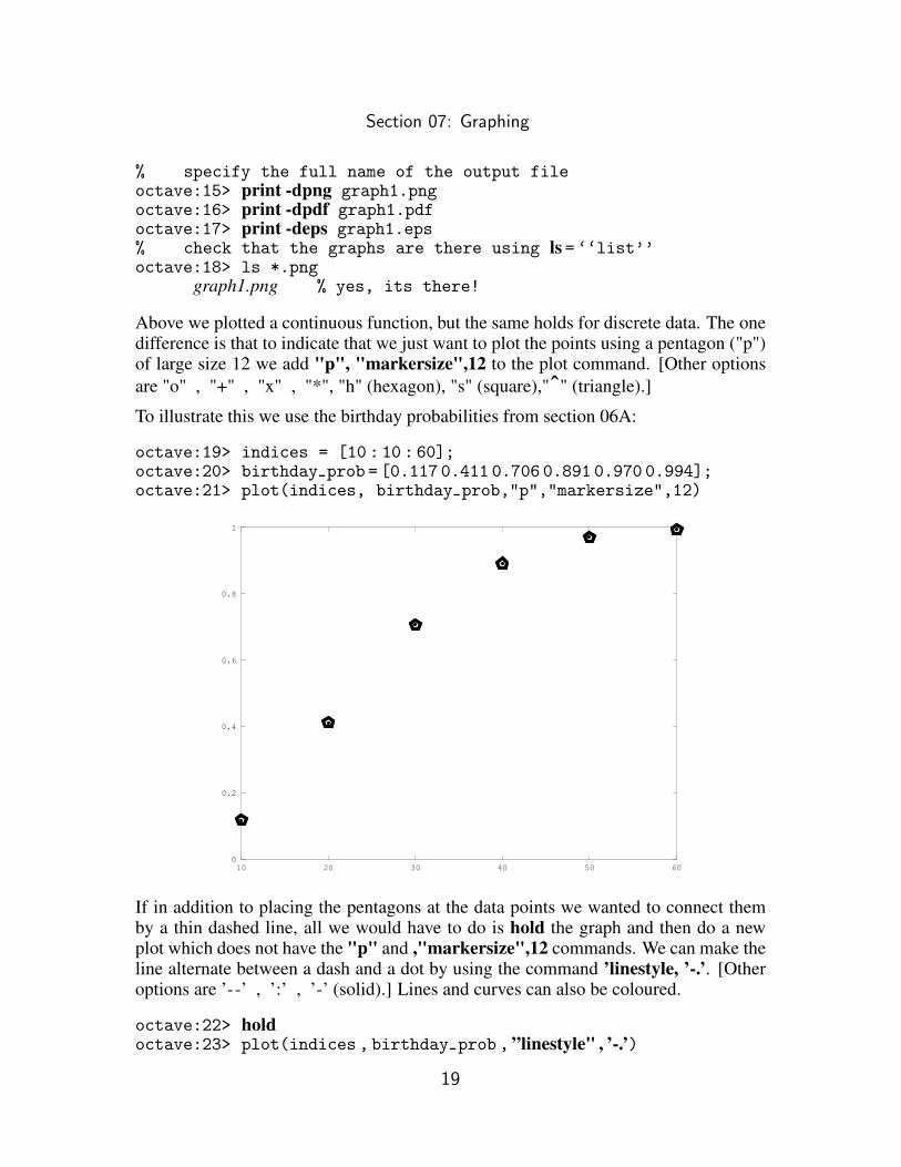
Above we plotted a continuous function, but the same holds for discrete data. The onedifference is that to indicate that we just want to plot the points using a pentagon ("p")of large size 12 we add "p", "markersize",12 to the plot command. [Other options

are "o" , "+" , "x" , "*", "h" (hexagon), "s" (square),"ˆ" (triangle).]

To illustrate this we use the birthday probabilities from section 06A:

octave:19> indices = [10 : 10 : 60];octave:20> birthday prob = [0.117 0.411 0.706 0.891 0.970 0.994];octave:21> plot(indices, birthday prob,"p","markersize",12)

0

0.2

0.4

0.6

0.8

1

10 20 30 40 50 60

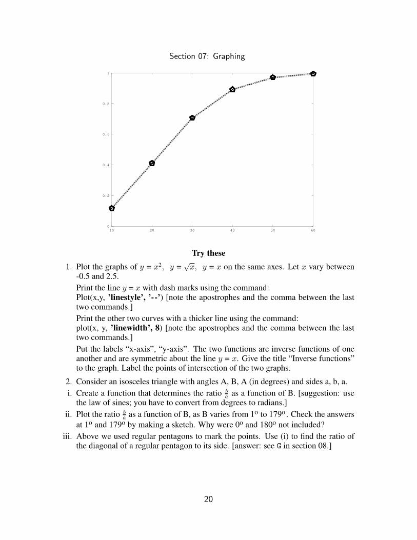
If in addition to placing the pentagons at the data points we wanted to connect themby a thin dashed line, all we would have to do is hold the graph and then do a newplot which does not have the "p" and ,"markersize",12 commands. We can make theline alternate between a dash and a dot by using the command ’linestyle, ’-.’. [Otheroptions are ’--’ , ’:’ , ’-’ (solid).] Lines and curves can also be coloured.

octave:22> holdoctave:23> plot(indices , birthday prob , ”linestyle" , ’-.’)

19


0

0.2

0.4

0.6

0.8

1

10 20 30 40 50 60

Try these

1. Plot the graphs of y = x2, y =√

x, y = x on the same axes. Let x vary between-0.5 and 2.5.

Print the line y = x with dash marks using the command:Plot(x,y, ’linestyle’, ’--’) [note the apostrophes and the comma between the lasttwo commands.]

Print the other two curves with a thicker line using the command:plot(x, y, ’linewidth’, 8) [note the apostrophes and the comma between the lasttwo commands.]

Put the labels “x-axis”, “y-axis”. The two functions are inverse functions of oneanother and are symmetric about the line y = x. Give the title “Inverse functions”to the graph. Label the points of intersection of the two graphs.

2. Consider an isosceles triangle with angles A, B, A (in degrees) and sides a, b, a.

i. Create a function that determines the ratio ba as a function of B. [suggestion: use

the law of sines; you have to convert from degrees to radians.]

ii. Plot the ratio ba as a function of B, as B varies from 1o to 179o . Check the answers

at 1o and 179o by making a sketch. Why were 0o and 180o not included?

iii. Above we used regular pentagons to mark the points. Use (i) to find the ratio ofthe diagonal of a regular pentagon to its side. [answer: see G in section 08.]

20

Section 08: Roots of a polynomial and zeros of a function

Polynomials

Suppose that we want to find a positive number such that the square is one more thanthe number. This leads to the polynomial equation:

x2 = 1 + x

and we want to find the roots. Since this equation is quadratic, we can use the quadraticformula, but what if we have a cubic or higher order polynomial? Octave has a routinefor finding the roots (or an appoximation) of any order polynomial.

The first step is to put all the terms of the polynomial on the left in decreasing order ofthe exponents:

x2 − x − 1 = 0

Now we create a vector whose entries are the coefficients of the polynomial:Then we use the Octave function roots ( ):

roots 1 = roots(poly 1)

octave:1> poly 1 = [1 -1 -1];octave:2> disp(poly 1)

1 -1 -1octave:3> roots 1 = roots(poly 1);octave:4> disp(roots 1)

-0.618031.61803

octave:5> G = (1+sqrt(5))/2;octave:6> disp(G)

1.6180

The calculation of step 5 shows that the desired solution of the quadratic equation

is 1+√

52 . This is the famous (and infamous) “golden number”.1 Other, surprising,

methods of finding G will appear in later sections.

Zeros of a function⋆

A quick sketch shows that for y ≥ 0 the line: y = x crosses the cosine curve at x = 0 andjust one other point. To find this point we first define the function my function4(x) =x − cos(x) and what we want to do is find the zeros of f4(x) . Octave has a functionfzero( ) which will find this root. So the next step is to write an “m-file” (section 03)which describes the function.

function y = my function 04(x)y = x - cos(x);

endfunction

To check for errors we evaluate the function at a few points:octave:1> my function 04(0)

ans = -1 % correct since cos(0) = -1

21

Section 08: Roots of a polynomial and zeros of a function

octave:2> my function 04(pi/2)ans = 1.5708 % this is π

2 as it should beoctave:3> pi/2

ans = 1.5708

[As in section 5, we can apply this function to a vector of values. This will be done inthe next section.]

Because my function 04(x) is negative at x = 0 and positive at π2 , the zero is someplace

between the two.

In general there may be many roots of a function, therefore we have to help Octave bygiving a starting point a. So the precise form of the command for fzero( ) is:

root1 = fzero(’my function 04’ , a)

Note the apostrophes on both sides of the name of the function, which is given withoutthe extension .m.

Since we know that the root lies between 0 and π2 , we can start with a = 1 as a guess:

octave:4> root1 = fzero(’my function 04’, 1)root1 = 0.73909

% check the answeroctave:5> my function 04(root1)

ans = 0

Try these

1. Find the roots of x2 = x + 12 by first using the quadratic formula and then usingpoly.

3. Find all the roots of x3 − 3x− 9x + 5 .

3. Find the square roots of 17 by setting up an equation and then using poly .

4. Find all the cube roots of 17. [the answer involves complex numbers as indicatedby the symbol i in the solution.]

5. What is the difference between 2−2x and 10x when x = 0; when x = 1? When arethey equal?

Cultural note

1. For a mathematical history see my book, A Mathematical History of Division in

Extreme and Mean Ratio, republished by Dover as A Mathematical History of the

Golden Number. For the infamous aspect see my book, The Shape of the Great

Pyramid and the articles on my web page: http://herz-fischler.ca .

22


Saving the answers

In the last section we defined the function my function 04(x) and evaluated it at thesingle point π

2 . As in section 05—where we worked with built-in functions—we canalso evaluate this function on a vector. Suppose we are interested in the values takenon by this function on the interval [π2 , π] and wish to find the approximate values of themaximum, minimum and average. To do this we use sub-intervals of length .01 (wecould use a much finer grid). We do this just as in section 06; note the semi-colon toavoid printing out all the values:

octave:1> x values = [pi:.01:2*pi];

Now we preceed in the same way as sections 05 and 08octave:2> y values = my function 04(x values);octave:3> max y value = max(y values)max y value = 5.2816octave:4> min y value = min(y values)min y value = 4.1416

Next we use the save command to save all the variables to a filed called example 4.dat.We then clear the work space and use the load command to re-obtain the variables.The command whos allows us to check (notice how the dimensions are given):

octave:5> save example 4.datoctave:6> clearoctave:7> whosoctave:8> load example 4.datoctave:9> whos

max y value 1x1min y value 1x1x 1x32x values 1x315y values 1x315

Now that we have the data again we can find the mean value:

octave:11> mean y value = mean(y values)mean y value = 4.7121

Counting the number of elments satisfying a certain condition

Consider the vector k3 = [ -1 -3 -5 -7 -9] of section 06. We want to know how many ofthe elements are greater than -4. In this case we can see right away that the answer is2, but imagine that we had measured the heights of 987 people and that we wanted toknow how many and what fraction of these 987 people were taller than 1.9 m. Octavelogic allows us to do the counting in two concise statements:

1. We make the “assignment” n3 = [k3 > - 4]. This is just shorthand for the action:“look at each of the elements of k3 and place a 1 in n3 if the corresponding elementof k3 is bigger than -4; otherwise put a 0”.

octave:1> k3 = [ -1 -3 -5 -7 -9];octave:2> n3 = [k3 > -4];

23


octave:3> disp(n3)1 1 0 0 0 only -1 and -3 are greater than -4

% the first two elements satisfy the condition%octave:4> l3= length(n3)octave:5> disp(l3)

5 % of course, since n3 has the same length as k3

2. In order to know how many of the elements of k3 are greater than -4 all we haveto do is count the number of 1s in n3 and to do this we can just take the sum of theelements of n3.

octave:6> s3 = sum(n3);octave:7> disp(s3)

2 % so 2 elements of k3 are greater than -4

3. Finally to find the fraction of elements of n3 which are greater than -4, we simplydivide s3 by the length of k3:

octave:8> fract3 = s3/l3;octave:9> disp(fract3)

0.40000 % 2 of 5 elements are are greater than -4

More logic with vectors ⋆

4. We can also impose multiple conditions using:& = “and”| = “or”Each condition is written separately inside ( ).

octave:11> k3 = [ -1 -3 -5 -7 -9];% how many elements of k3 are > -4 and also < -2octave:12> m3 =[(k3 > -4) & (k3 < -2)];octave:13> disp(m3)

0 1 0 0 0 % only element 2 satisfies both conditionsoctave:14> disp(sum(m3)) % note the double ( )

1

Try these

1. How many elements of the sequence{

-5, 1 , -1 , 4, 0}

are either less than -2 orstrictly positive?

2. “less than or equal” is written <=. Repeat (1) with “strictly positive” replaced by“non-negative”.

3. ⋆ Redo steps 11 and 12 if and is replaced by or.

4. ⋆ To test for equality Octave uses = = (two equal signs as distinquished from“assignment” statements such as n3 = [k3 > -4]. How many elements of thesequence

{

4, 3, -2, 4, 1}

are exactly equal to 4?

5. ⋆ “not equal” is written ˜ =. How many elements of k3 are not equal to -7?

24


In section 04 we discussed the concept of a vector which is simply a row1 (or 1-dimensional set) of data. Amatrix extends this idea to rectangular (or 2-dimensional)sets of data. For example:

M =[

1 2 34 5 6

]

is called a 2 by 3 matrix, with the first number always referring to the number ofrows. It is good practice to designate vectors and variablesby lower case letters (e.g.vector , x) and matrices by upper case variables (e.g.M).

Entering the data for matrices

To enter the data we simply start typing and then, at the pointwhich marks the endof the data for the first line, we put a semi-colon. Note that this is a different use ofsemi-colons from their use in suppressing printing.

% all the data can go on one line.% indicate the separation between the rows by a semi-colonoctave:1> M = [1 2 3 ; 4 5 6]

M =1 2 34 5 6

We could also place the data on two lines. After the first line we need to put three dotsto indicate that we are continuing. The same thing would be done if the rows of thematrix were too long to fit on one line.

octave:2> M = [1 2 3; ... % ⇐= three dots> 4 5 6] % we continue the input on the next line

M =1 2 34 5 6

Building matrices from vectors

Suppose that we have four candidates for a position and we give each of them a batteryof three tests, with test 1 being worth a maximum of 30 points,test 2 being worth amaximum of 50 points, and test 3 being worth a maximum of 20 points. We place thescores of each candidate in a vector:

octave:1> candidate 1 = [21 34 15];octave:2> candidate 2 = [29 14 9];octave:3> candidate 3 = [16 41 17];octave:4> candidate 4 = [21 32 18];

To form a matrixCANDIDATES we place the four vectors inside[ ] and separate themby semi-colons. Because the names are long we put... after the third vector (to indi-cate that we are going to continue) and then go on to the next line:

25


octave:5> CANDIDATES = [candidate 1;candidate 22; candidate 3; ...> candidate 4]% as a check we let Octave print, so there is no ; after the [ ]%

CANDIDATES =21 34 1529 14 916 41 1721 32 18

Statistics, part 2

Now we want to find the mean and standard deviation on the tests. Since therowsof CANDIDATES represent distinct people, whereas thecolumns correspond to distincttests, we want to find the means and standard deviations of thecolumns. Because ofthis kind of situation, Octave functions such assum, max, mean etc., operate on thecolumns of a matrix and not on the rows.

octave:6> test averages = mean(CANDIDATES);octave:7> disp(test averages)

21.750 30.250 14.750%octave:8> test std = std(CANDIDATES);octave:9> disp(test std)

5.3774 11.5000 4.0311%octave:10> max on each test = max(CANDIDATES);octave:11> disp(max on each test)

29 41 18

Note

1. There are alsocolumn vectors and then one uses the terminologyrow vector insteadof just vector.

Try these1. Create the following vectors using the index method of section 06:

v 1 = {2, 4 ... 16} ; v 2 = {-3, -6 ...-24}; v 3 = {1, 3 ... 7} .Check, usinglength( ), that the lengths of all three vectors are the same.

2. Form a matrixM2 from v 1, v 2 andv 3.Find the dimensions ofM2 using the Octave commandsize( ).Find the minimum value in each column ofM2.

26


Suppose that we have the simultaneous equations:

2x− 3y = 1

x + 2y = 4

[Check out the following steps on a piece of paper.] To solve these we would first notethe 1x in the second equation and so we would switch the two equations. Then wewould subtract 2 times the new first equation from the new second equation. Next we

would divide the second equation by −7. Finally we would subtract 2 times the secondequation from the first equation. These steps would result in the following reduced (orequivalent) equations:

1x + 0y = 2

0x + 1y = 1

From these reduced equations we can simply read off the solutions, x = 2, y = 1 andthen—of course—we would check the solutions in the original equations.

In these manipulations we only used x,y to make sure that we were working withthe right numbers (to see this, just suppose that the second equation had been written2y = 4 − 2x).

So we might just as well write the equations in matrix form, with the first column

representing the coefficients of x, the second column representing the coefficients ofy and the third column representing the constants. [For emphasis the constants areseparated from the variables by a vertical bar.]

[

2 −3 | 11 2 | 4

]

Now repeat exactly the same sequence of manipulations on the rows of the matrix that

we performed on the equations :[

1 2 | 42 −3 | 1

]

[

1 2 | 40 −7 | −7

]

[

1 2 | 40 1 | 1

]

[

1 0 | 20 1 | 1

]

From this final matrix we again see that x = 2, y = 1.

27


The process that we went through to obtain the reduced equations, is variously called“row reduction”, “reduction to row echelon form”, “Gauss-Jordan reduction”, the

“pivot method” etc, .

Doing this is tedious, to say the least, especially if there are three or more equationsand non-integer coefficients. Fortunately this is the type of calculation that computerscan do quickly, efficiently, and—most importantly—correctly. Octave has the built in

command rref( ) which does the work for us.

octave:1> M1 = [2 -3 1; 1 2 4]

M1 =2 -3 11 2 4

%octave:2> solution M1 = rref(M1)

solution M1 =1 0 20 1 1

The same procedure would be followed in case there were more variables than equa-tions (usually implying an infinite number of solutions where at least one of the vari-ables is treated as a “constant”), or in case there are more equations than variables(usually implying that there are no solutions). The interpretation of the answers in

these two cases becomes more involved.

Try this

1. Solve, first by hand and then by using using Octave, the equations:

2x− y = 2

x + y = 7

2. Solve, first by hand and then by using using Octave, the equations:

2x− y + z = 2

x + y − z = 7

x + y + 2z = 4

This problem is done by another method in section 20.

28


A program is simply a set of Octave instructions. Often we want to repeat an operationmany times and instead of constantly recomputing individual quantities we create aprogram which contains a "for-loop". This consists of a statement of the form:for k = [set of indices]

instructions to do somethingendfor

[Note thatendfor is written asone word, and not two words, “end for”.for andendfor are in lower case letters. We saw the same thing in section 02,where we wroteendfunction]

Do not usei or j as the symbol for the indice as these are reserved for√

−1.

To create a program we place the instructions, including thefor-loop, inside an “m-file”. For illustrative purposes, suppose we want the squares of the first five integers.Here is a program to do this; note the use of a semi-colon at line 3 anddisp( ) todisplay the answer:

% [for loop 01.m]for k = [1:5]square = (k).ˆ2 ;disp(square)endfor

To execute this program we go to the Octave prompt and type “for loop 01”. withoutthe extension .m.

octave:1> for loop 01 % name of the program1491625

Two things should be noted:i. For this simple example we could have obtained the answer using element by ele-

ment powers of a vector:octave:2> k = [1 : 5];octave:3> powers = (k).ˆ(2);octave:4> disp(powers)

1 4 9 16 25In more complicated situations (section 13A) both vectors and loops will be used.

ii. Octave prints out the answers one at a time. This can be very inconvenient if weare displaying many answers. To get around this we first storeall the answers in avectorstore and only displaystore at the end.

29


Storing values

Since vectors are just collections of numbers, the individual elements can be displayedby means of the index. Thus ifa is a vector then the third element isa(3):octave:5> a = [7 -2 5 4];octave:6> a(3)

ans = 5

Now we want to create a vector of zeros that has the same lengthasa. In the aboveexample we could count, but suppose we had a large vector of data. We use the functionlength(a), but there is no need to display the value. We then create a vector storewhose length is the same as that ofa.

octave:7> l = length(a); % no need to display the valueoctave:8> store = zeros(1 , l)

store = 0 0 0 0

Next we change the value of the third element of store from 0 to8, by settingstore(3)= 8.

octave:7> store(3) = 8; an ‘‘assignment’’octave:8> disp(store)

0 0 8 0

If we use this technique in a for-loop, then all we have to do atthe end is writedisp(store). We could also writemean(store) if we wanted the mean etc.

Other sets of indices

In the for-loop above our index set was1 : 5, Octave will acceptany set of indices.Try out the following sets:

% [for loop 02.m]for k = [10 : -2 : 5] % or [3 5 7 11 13]

square = (k).ˆ2;endfor

Try these

1. Run [for loop 02.m]. What are the values for which the square is evaluated?

2. Run [for loop 03.m]. What are the values for which the square is evaluated?

3. Write a program that has the statementstotal = 0 and a = [7 -2 5 4]before theloop begins. Now loop 4 times. At step k evaluatea(k) and adda(k) to total,by means of theassignment:

total = total + a(k)[In an assignment the internal counter fortotal replaces the value on the right,by the new value on the left.]At the end of the 4 loops, display the value oftotal and compare it tosum(a).

30


The new elements in the following program are:i. before we start the loop we assigninital values to two quantities,a andb.

ii. each time we loop we change the values ofa andb.

% [fibonnaci.m]%% initial values

a = 1;b = 1;

%% loop 10 times, each time:% 1. find the ratio b/a% 2. add a+b = c% 3. b becomes the new a% 4. c becomes the new b%% we want to store the values (section 12)

store ratio = zeros(1,10);store sum = zeros(1,10);

for k = [1 : 10]

ratio = b/a;store ratio(k) = ratio;

%c = a+b;store sum(k) = c;

%% now assign new values to a and b

a = b; % do this first, before b changes!b = c;

endfordisp(store sum)disp(store ratio)

We now run the program:octave:5> fbonacci % the name without the extension .m% the output is:

1 1 2 3 5 8 13 21 34 55 89 1441.0000 2.0000 1.5000 1.6667 1.6000 1.62501.6154 1.6190 1.6176 1.6182

%% switch to the high precision displayoctave:6> format long

31


% display the last ratiooctave:7> store ratio(10) the 10th element of store ratio

1.61818181818182 % the repeating infinite series = 1.6182% we can check, the last ratio should be 89/55octave:12> 89/55

1.61818181818182%% recall the ‘‘golden number’’ of section 08.octave:8> G = (1+sqrt(5))/2;octave:9> disp(G)

1.61803398874989

The sequence{1 1 2 3 5 8 13 21 34 55 89 144...} is called the Fibonacci1 sequence. Theratios become closer and closer toG, alternating between less than and greater thanG.

Note

1. Fibonacci was active ca. 1200. He presents the sequence which bears his name inconnection with the “rabbit problem”. Despite the fact thathe was in command ofthegeometrical properties of the golden number, there is no indication thathe wasaware of the connection. For a discussion, see my book listedin the note to section08. It is possible that Fibonacci learned about the “rabbit problem” from the Arabworld.

Try this

1. Start with 1. Next compute:

1 +11

then:1 +

11 + 1

1

then:1 +

11 + 1

1+11

...

i. Take a guess as to what will happen when we continue the process. [hint: thereis no need to give you a hint!]

ii. Write a program to compute the first ten values and then compare the result ofyour computation with your guess.

note: This example belongs to the beautiful theory ofcontinued fractions. If wereverse the process and find the continued fraction of an irrational number, e.g.π, then we can find the successive “best”rational approximations to the irrationalnumber. Forπ the successive “best” approximations are3

1, 227 , 333

106,355113,

10399333102 . This

last rational is equal to 3.14159265358979, with an error estimate of 11099482930.

32


Sometimes we want to test a series of numbers, or a vector, or amatrix to see if certainconditions are satisfied. In Octave the testing is done viaconditional statements. In itssimplest form a conditional statement looks like:if state the condition

state what to do if the condition is satisfiedendif[note that the closing isoneword: endif, not “end if”]

Conditional statements can appear in functions as well as inprograms. Here is a simpleexample; we want to write a function which will test if an integer is divisible by 27.Here we use thefloor function [greatest integer function] of section 02. If a numbern is divisible by 27 then there is no remainder and sofloor(n/27) = n/27. If thiscondition is satisfied then the function prints outn andn/27. [The statement “j =” isnot really needed here; it is put in order to follow the function format of section 03.]

% [if simple.m]%function j = if simple(n)% state the condition

if floor(n/27) == n/27 % double == for equality

% state what to do if the condition is satisfieddisp(n), disp(n/27)

%

endif % completes the conditional statement

endfunction

We run the program, first with 54 and then with 271. For 271 the condition associatedwith if is not satsified so nothing happens.

octave:10> if simple(54)542

octave:11> if simple(271)octave:12> % nothing has happened, so the next prompt appears

If we wanted something to happen whenn = 271 we could add anelsestatement forthe cases when the condition of theif statement isnot satisfied:

% [else simple.m]function j = else simple(n) %

if floor(n/27) == n/27 % double == for equality

disp(n), disp(n/27)

33


% say what to do in the alternate (else) case:else disp(n), disp(ceil(n/27))

endif % just one end statement for both if and elseendfunction

If instead of just an alternative to theif condition, we had a second condition, we wouldreplaceelseby elseif, e.g.:

elseif floor(n/18) == n/18disp(n), disp(ceil(n/18))

% we might perhaps want another elseif statementelseif fix(n/96) == 0

disp(n+24)

We can have as manyelseifstatements as we need, but at most oneelsestatement.

Input from the keyboard

When writing a program that will be used for many different input values, it is useful tobe able to supply the data externally. This might happen if wegenerated the elementsof a vector or matrix via one program and then wanted to perform calculations on thevector or matrix. A typical input statement would look like this [note the semi-colon]:

keyboardvector =input( ’ What is the vector, eh? ’);

As an example we tranform the abovefunctionif simple( ) into aprogramwith input.The statementsfunction andendfunction no longer appear. [Do not use “input” aspart of the name as it is a reserved function.]

% [simple keyboard.m]%n = input( ’ What is the number, eh? ’);% [N.B. the Canadian shibboleth, ‘‘eh’’ is optional]% the rest of the program is identical to [if keyboard.m]if floor(n/27) == n/27 % double == for equality

disp(n), disp(n/27)

endif

Try these

1. Check the first 99 integers to see if they are squares. If theanswer is yes. print outthe integer and its square root. Repeat using theinput of a numbern.

2. Consider all the multiples ofπ4 on the interval [0 ,1]. Check which of the followingmutually exclusiveconditions are satisfied:

i. the cosine is an integer not equal to 0.ii. the cosine is equal to 0.

iii. the cosine is a negative number, but not an integer.

34


In some situations we can not determine in advance how many times we want to loopbecause we want to keep going until a certain condition is met. In such cases awhileloop is very useful. In the first example we start withk = 5 and we want to find the lastvalue ofk such that the square is less than or equal to 98.

The hitch is that we have to go above 98 to know when to stop. This is the time tothink mathematically; if a certain value ofk puts us above 98, then the value that wewant isk-1. That is why,after we exit the while-loop we set the variable lastk= k-1.

A technical feature that we now add is the display ofalphanumeric text. The text thatis to be displayed is enclosed between two apostrophes:disp(’the output =’).

% [while square.m]

% while-loops do not have a set of indices as in for-loops% rather we provide an initial value, in this case 5

k = 5;%% we now write while followed by the condition

while (k)ˆ2 <= 98

k = k+1; ‘‘increment’’ the index value

endwhile% at this point we have broken out of the while-loop% the last value of k put us over 98 so we go back to k-1

last k = k-1;

% now we give the commant to display the answers

disp(’last k for which square<= 98’), disp(last k)

We run the program:octave:1> while square

last k for which square <= 98 % alphanumeric output9 % numerical answer

More interesting examples involve continuing until we are within a certain tolerance.In section 13 we generated ten Fibonacci numbers and their ratios. We saw that theratios came closer and closer to the golden number. Now we aregoing to keep goinguntil we are within .00001 of the golden number. To do this we modify [fibonacci.m].

% [fibonacci while.m]%% initial values

a = 1;b = 1;ratio = 1; % we now also need a seed value for ratio

%G = (1 + sqrt(5))/2; the ‘‘golden number’’ (section 08)

35

Section 15: While loops; alphanumeric texts

% each time that we might reenter the loop we check if the% difference is within .00001 = 10−5

while abs(ratio - G) >= 10ˆ(-5) % use the absolute value to check

% for clarity we save a and b under new namesprevious a = a;previous b = b;

%% we add: ‘‘previous a’’ to ‘‘previous b’’ to obtain ‘‘new sum’’% ‘‘previous b’’ becomes the ‘‘a’’ for the ratio% ‘‘new sum’’ becomes the ‘‘b’’ for the ratio

new sum = previous a + previous b;%

a = previous b; % a for next loop; do before b changes!b = new sum; % b for next loop;

% find the new ratio b/aratio = b/a; % to test the program take off the semi-colon

endwhile%

disp(’Fibonacci 1 = ’), disp(a)disp(’Fibonacci 2 = ’), disp(b)format longdiff = abs(ratio - G); % check the differencedisp(’difference = ’), disp(diff)

We run the program:octave:22> fibonacci while

Fibonacci 1 = 233Fibonacci 2 = 377 % before 2, 3, 5 . . .55, 89; now 144, 233, 377

difference = 8.23767693347577e-06

Try these1. If we keep taking the square roots of a positive number, theroots will become

closer and closer to 1. Write a program that asks for an input value and stops afterwe are within .001 of 1. Output the number ofiterationsneeded.

2. In section 08 we saw thatG satisfiesx2 = 1 +x. Taking the square root of bothsides we see thatG also satisfies:

x =√

1 +x =√

1 +√

1 +x =

√

1 +√

1 +√

1 +x . . .

So if we calculate:

x =√

1 + 1 =√

1 +√

1 + 1 =

√

1 +√

1 +√

1 + 1 . . .

we will come closer and closer toG. How many times do we have to repeat theprocess so as to come within .0001 ofG? Repeat for question 1 of section 14.

36

Section 15A⋆: Pick a number, part 2

In section 06A we saw how to calculate the probability that if k people pick a numberfrom {1, ,2 ... n}that at least two will pick the same number. We did the calculationsfor the “birthday problem” where n = 365 and for k = 10, 20, ... 60 . In question 1 youwere asked to modify the birthday problem for arbitrary n.

All this was nice in theory, but suppose you wanted to try it out on a group of 30.The probability that two people out of the 30 have the same birthday is only .71. Thismeans that about 29% of the time you would look pretty silly. With 25 people theprobability is down to .57 and so about 43% of the time all the people in a random testgroup would have different birthdays.

What we want to look at is the inverse “birthday problem”, namely for a given numberof people k, how large can n be so that we have a degree of certainty that at least two

will be the same number. There is no direct way of computing this maximum value ofn, but this is not a problem; we “guess” n and let the computer check if we have gonebelow the chosen degree of certainty. If not, we guess again by increasing the value ofn by 1.

In practical terms we use a while-loop as in the last section. As input values we givethe value of k and the tolerance value. The intermediate calculations are the same asin section 06A.

% [pick number 01.m]%k = input(’how many people will pick a number? ’);p1 = input(’input you tolerance: .5, .75, .90, .95, .99? ’);%

p2 = 1 - p1; maximum allowable value for prob all different%

n = k; % starting value for nprob all different = 0; % approximate probability when n = k

%while prob all different < p2%% increment n by 1 for this new loop

n = n + 1; % assignment for new na = [n: -1 : (n-k+1)]; % index vector [n, n-1, ... (n-k+1]

% divide each element of a by n and multiply all the termsprob all different = prod((1/n)*a);

%endwhile%% once prob all different >= p2 we have gone too% far so the desired answer is n-1

disp(’k =’), disp(k), disp(’people’)disp(’tolerance =’), disp(p1)disp(’maximum n is’), disp(n-1)

37

Section 15A: Pick a number, part 2

We now run the program for k = 100 people and with tolerance levels of .99, .95, .90,.75, 50 .

tolerance = .99 maximum n = 1108





Notice how quickly the maximum value of n climbs with decreasing tolerance. If weuse .95 we can ask 100 people to pick from {1, 2, ... 1685} and be certain 95% of thetime that at least two people will pick the same number. If we want virtually absolutecertainty (99% of the time) we can still go up to 1108. This is much higher than anyonewould guess ahead of time.

Instead of calculating the maximum value for a fixed number (100) of people and dif-ferent values of the tolerance, we could fix the tolerance and calculate the maximumvalue for different numbers of people. If we do this for tolerance = .99 (virtual cer-tainly), then for 10, 20, ... 100, we obtain the values: 13, 48, 104, 183, 283, 404, 548,713, 900, 1108.

The last number, 1108, is the same as above because the calculation is the same.

Try these

1. We saw in section 06A that for 50 people, the probability that at least two peoplehave the same birthday is .970, where as for 60 people we are at .994. We can lookat the inverse problem: What is the least number of people so that the probabilitythat at least two have the same birthday is greater than or equal to .99? Findthis number by using pick number 01 with tolerance = .99 and k = 50, 51, ... 60people. [solution: at some point the maximum value will go from below 365 toabove 365. we want to find the the smallest k for which we are above 365.

2. Plot the maximum values obtained in (1) against k = 50, 51, ... 60 people. Drawthe horiziontal line n = 365. First draw the points discretely using squares of size10 and then connect them using a dotted line of thickness 4; see the examples insection 07 (graphing). Label the point where the graph crosses the horizontal line.Give appropriate titles to the x-axis, y-axis and your graph.

38

Section 16⋆: Binomial coefficients and probabilities

Rosencrantz: Heads.

(He picks it up and puts it in his bag. The process is repeated.)

Heads.

(Again.)

Rosencrantz: Heads.

(Again.)

Heads.

(Again.)

Guildernstern (flipping a coin): There is an art to the building up of suspense.

— Tom Stoppard, Rosencrantz & Guildenstern Are Dead, Act One.

Suppose that a weighted coin has a probability .4 of coming up heads and that we flipthe coin 5 times. We want to find the probability that we will have exactly 2 heads and3 tails in the 5 tosses.

There are several ways in which this can happen: we could have the sequence {H HT T T}, or the sequence {H T H T T} etc.. If you list all the ways of having exactly 2heads and 3 tails in 5 tosses you will see that there are indeed 10 possibilities.

Where does the number 10 come from? We can reason as follows: we can think ofthe tosses as “slots” and the 2 heads as “objects” to place in 2 of the 5 slots. For thefirst head we have the choice of 5 slots and for the second head we have the choice of4 slots. That makes 5 x 4 = 20 possibilities. But this is not the correct answer becausethe 2 objects (i.e. the 2 heads) are identical. So we have to divide 20 by the 2 x 1 = 2!(2 factorial) = 2 duplications. So:

number of distinct ways of having 2 heads in 5 tosses =5 × 4

2 × 1= 10

Because of the way it arises, the calculated quantity is referred to as “5 choose 2”.These same numbers also appear in the binomial expansion and so are also referredto in general as the “binomial coefficients”. There are different symbols for these

including(

52

)

and C(5,2). If we toss n times, then the number of ways in which we

can have k heads is given by:

n choose k =

(

n

k

)

=n× n− 1 × . . . (n− k + 1)

k!

Octave has two functions, for the two names, nchoosek(n , k) and bincoeff(n , k) ofevaluating the binomial coefficients:

octave:7> nchoosek(5,2)ans = 10

octave:8> bincoeff(5,2)ans = 10

39

Section 16: Binomial coefficients and probabilities

Now we want to find the probability of exactly 2 heads in 5 tosses. Since the weightedcoin has a probability .4 of coming up heads on any particular toss, the probabilityof tails is .6. So for any particular sequence (e.g. {T H H T T}) the probability is.4 × .4 × .6 × .6 × .6 .

Since there are 10 possible sequences involving exactly 2 heads and 3 tails we have:

probability of exactly 2 heads in 5 tosses = 10 · (.4)2 · (.6)3 =

(

5

2

)

· (.4)2 · (.6)3

This is called the binomial probability. The general formula, when the probability ofheads on one toss is p and the probability of tails on one toss is q = 1 − p is:

probability of k heads in n tosses =

(

n

k

)

· (p)k · (q)n-k

Octave has the function binopdf(k , n, p) to evaluate the binomial probabilities; notethat the number of heads k comes first, then number of tosses n. [pdf stands for“probability distribution function”]

octave:1> p2 = binopdf(2 , 5, .4)octave:2> disp(p2)

0.34560

Try these

1. Instead of counting the number of ways we can have 2 heads in 5 tosses, we couldcount the number of ways we can have 3 tails in 5 tosses. The number of waysmust be exactly the same because if we have 2 heads then we have 3 tails and ifwe have 3 tails we must have 2 heads. If you are convinced by the previous twosentences of this paragraph then what result have you just proved?

2. Above we computed the probability of exactly 2 heads. Call this probability p2.Do the same for 0, 1, 3, 4 , 5 heads. Call these probabilities p0, p1, p3, p4, p5. Addup all the probabilities. What result have you just proved?

3. When people in France come into a room they shake hands with all the otherpeople. If there are 24 Francais in a room, how many handshakes will there havebeen by the time they have finished? Suppose that they change the custom andhave three people at a time clasp hands?

4. Use prod( ) to create our own choice function of two variables: choice(n , k).

40

Section 17⋆: Tossing coins on a computer, part 1

We understand intuitively what tossing a coin “at random” means, but defining it pre-cisely is a different story. In fact no one has ever been able to give a completely rig-orous mathematical definition of “randomness”. Instead oneuses a series of statisticaltests to check if there is no reason to reject a certain phenomena as being “random”.

Random phenomena, such as coin tossings, aresimulated on computers by means ofrandom number generators.1

Terminology: Computer generated random numbers are elements of a very large set ofnumbers{xk}such that 0< xk < 1.

To output random numbers Octave has the commandrand(1, n) which will generate arandom vector of lengthn. Here is the output if we generate 10 random numbers :octave:1> random 01 = rand(1, 10);octave:2> disp(random 01)

0.700931 0.501059 0.344372 0.565966 0.4297730.126794 0.013282 0.684946 0.486618 0.864318

If we repeated the same command we would obtain anew set of 10 random numbers.⋆⋆ We can reobtain the same set if we reset the seed , e.g. 45834, each time, using thethe command:rand(’seed’, 45834). This feature is important for testing simulations.

In section 06A we discussed coin-tossing with a weighted coin that had a probability.4 of coming up heads. To explain how we simulate tossing thiscoin, consider thefollowing diagram:

H T

0 .4 1

The interval [0 .4] has length .4 and so takes up 40% of the interval [0 1]. If thenumbers that we generateact as if they were generated at random then we wouldexpect that about 40% of them would lie in the interval [0 .4].If we generate 1000random numbers and then count how many (using the vector logic of section 08) ofthem fall in the interval [0 .4], then we would expect that theanswer is somewherenear 400. If we then divide the number by 1000 we will have therelative frequency(also called theempirical probability) of “heads”. In turn the relative frequency shouldbe close to thetheoretical probability which is .4.

To illustrate, via a short example, we first generate 6 randomnumbers:octave:1> a = rand(1 , 6);

0.89997 0.32240 0.82164 0.58678 0.91927 0.28393

To test for “heads” (i.e. which random numbers are <= .4), we use vector logic [section09]. We let vectorb= [a<= .4]. Octave places a 1 inb wherever the correspondingrandom number in vectora is <= .4. Check this visually by looking at the randomnumbers just above and then the 1s just below:

41

Section 17: Tossing coins on a computer, part 1

octave:2> b = [a<=.4]0 1 0 0 1

To find the number of “heads”, we simply add the 1s.octave:3> c = sum(b)

2

Finally we find the relative frequency of “heads” by dividingc by 6.octave:4> relative frequency = c/6

0.33333

Now we do exactly the same thing for 1000 “tosses”, by generating 1000 randomnumbers:octave:5> e = rand(1 , 1000); % Do not forget the semi-colon!%octave:6> f = [a<=.4];octave:7> g = sum( )

ans = 392octave:8> relative frequency = g/100

relative frequency = = 0.39200 % this is ‘‘close’’ to .4

Notes

1. The usual—new methods are always being developed—technique used to generatethe random numbers is “modular arithmetic”. This can be illustrated by thinking ofa twelve hour clock. We start with 2 as a “seed”. Then we use 5 asa “multiplier”:2· 5 = 10. We divide by 12:10

12 = 0.83336 and this is our first random number.Now we multiply 10· 5 = 50 = 4· 12 + 2, i.e. we have gone around the clock fourtimes and we are now at 2 o’clock. We again divide by 12:2

12 = 0.1666 and thisis our second random number. But 2 was the original seed so if we continue weagain obtain 10! This is certainlynot random!Finding the right values for the seed, multiplier and divisor is not an easy task es-pecially since simulations require millions, billions, even trillions (atomic physics)of random numbers which do not repeat. Finding a good random number generatoris both a science and an art. Octave (version 3.6.3) uses a generator with a periodof 219937−1. [Use logarithms to express 219937−1 as a power of 10. If you try toevaluate this number in Octave, the answer will be “infinity”.]

Try these

1. Generate a 1000 random numbers and determine what fraction lies between .55and .82. [Use step 4 of Section 09.]

2. Convince yourself by a few numerical examples that ifx is a random number andN is an integer, then the formula:

j = 1 + floor(N ·x)will give a random integer from the sequence{1, 2, ...N}.Use this formula with N = 6 to simulate tossing a die 1000 times.

42

Section 18⋆⋆: Tossing coins on a computer, part 2

“ ‘I’ll tell you what,’ said Mr. Bumblemoose when Joachim hadstopped read-ing, ‘he’s one of those new-fangled Professors who think youcan prove every-thing with a computer. What do all those rows of figures and statistics mean tome? Nothing at all! These new-look Professors are just witch-doctors, but theydo it with a row of figures and make you so dizzy that in the end you believeeverything they tell you. But I don’t believe it! ’”

— Hans Andreus, “Mr. Bumblemoose Quarrels with Joachim”, inMr. Bumblemoose and the Mumblepuss, London: Abelard-Schumanan, 1973(original Dutch version, 1968), p. 29.

In section 17 we tossedonecoin, with the theoretical probability of heads ononetossbeing .4. When we repeated this experiment 1000 times therelative frequency of heads(or empirical probability) was close to thetheoreticalprobability. Now we return tosection 15 where we tossed the same coin 5 times, with the probability of 2 heads in 5tossesbeing given by the binomial distribution.

The idea is the same as in section 17, but now instead of generatingonerandom numberat a time, we generatefive random numbers at a time. This will be referred to asthe basic experiment. Next we repeat thebasic experiment1000 times. Instead of a1×1000vector, we now are going to have a 5×1000matrix. The Octave logic remainsthe same for matrices as for vectors.

To illustrate, here is a 6 time repetition of thebasic experiment. What makes thissimulation more complicated is that we first have to add the number of 1s in eachcolumn (i.e. count the number of heads in 5 tosses). This results in avectorc. Thenwe have to use Octave logic a second time to find out which elements of thevectorcare equal to 2 (i.e. which of the 6 repetitions resulted in exactly 2 heads).

Check this visually by looking at the random numbers inA and then the 1s inB:

octave:1> A = rand(5 , 6) capital letters for matrices

0.763913 0.253032 0.357587 0.091995 0.120525 0.6383360.933027 0.764294 0.532767 0.178103 0.944216 0.2991170.794544 0.332849 0.814172 0.594680 0.025912 0.6445700.838468 0.488249 0.449008 0.250096 0.533096 0.0526260.077102 0.439889 0.798099 0.583340 0.955996 0.466741

%octave:2> B = [A <= .4]

0 1 1 1 1 00 0 0 1 0 10 1 0 0 1 00 0 0 1 0 11 0 0 0 0 0

43

Section 18: Tossing coins on a computer, part 2

% now we add the columnsto see how many heads% check the column sums by handoctave:3> c = sum(B)

1 2 1 3 2 2%% which elements of c equal 2?octave:4> d = [c== 2] % note the double equal sign% check that the 1s in vector d match up with the 2s in vector c

0 1 0 0 1 1%% now add up the ones in c to find out% how many times we had a 2 in coctave:5> e = sum(d)

3%% finally the relative frequencyoctave:6> f = e/6

0.50000

We do exactly the same thing for 1000 repetitions and comparewith the binomialdistribution of section 15.

octave:7> A = rand(5 , 1000);octave:8> B = [A <= .4];octave:9> c = sum(B);octave:10> d = [c== 2];octave:11> e = sum(d);octave:12> f = e/1000

0.34300octave:2> binopdf(2 , 5, .4)

0.34560

Try this

1. Reconsider problem 2 of section 17. Suppose that we toss the die 7 times. Whatis the theorical probability ofexactlyone four? Use Octave to simulate this basicexperiment 500 times and find the empirical probability ofexactlyone four in 7tosses.

44

Section 19: Statistics, part 3; Histograms

A wide variety of data appears to follow the normal distribution (often loosely re-ferred to as the “bell-shaped curve”) . For the purpose of providing data we want togenerate normal random numbers with mean = 0 and standard deviation =1. To ob-tain these numbers we use the function randn(n , 1). Here n is the number of normalrandom numbers that we want to generate. To have a large sample, we generate 8261random normal numbers [be sure to put a semi-colon, to suppress printing, after eachstatement]:

octave:1> x = randn(8261,1);% we check the mean and standard deviation (section 05)octave:2> mean(x)ans = 0.011881 % theoretical value = 0octave:3> std(x)ans = 0.99582 % theoretical value = 1

The next step is to use x to obtain values with a mean of 1.42 and a standard deviationof .31. To do this we multiply all values in x by the desired standard deviation andthen add the desired mean:

octave:4> y = .31*x + 1.42;% we check the mean and standard deviation (section 05)octave:5> mean(y)ans = 1.4237 theoretical value = 1.42octave:6 > std(y)ans = 0.30870 theoretical value = .31

We are now ready to find the histogram. The command is hist(y groupings). Herey is the data that we want to analyse and groupings is the number of divisions ofthe data that we wish. Deciding the number of groupings is partially a question oftrial-and-error; here we try 15 groupings with the vector obtained in statement 4:

octave: 7> hist(y 15)

Now we are ready to obtain the graph (section 07; we could have also printed directlyto a PDF file):

octave:8 > print -dpng normal [mean-1.42--std-.31] [15-bins].png

Notice how the graph is more or less centred about the desired mean = 1.42. If we hadused a much larger data set and a larger value for the number of groupings we wouldbe closer to the normal curve.

For the normal curve about 95% of the area is within 2×std of the mean. In our casethis would mean between approximately 1.4 + .6 = 2 and 1.4 − .6 = 0.8 and visuallythis does not seem unreasonable. Only a more sophisticated test (e.g. the chi-squaredtest) would determine how close the histogram is to the normal curve

We obtain the following graph:

45

Section 19: Statistics, part 3: histograms

Try these

1. Repeat the above with a mean of -2.6 and a standard deviation of 4.9. Generate9,416 normal random numbers. Try with several different values for the numberof groupings.

2. Use the ordinary random number generator of section 17 and exercise 2 of thatsection to simulate 5000 tosses of a die. Obtain a histogram with 10 divisions.

46


In section 10 we saw how to enter data for matrices and how to build matrices fromvectors. Then in section 11 we discussed the relationship between matrices and equa-tions. Here we continue the discussion and introduce new operations on matrices. Insection 10 we spoke of a 2 by 3 matrix. We also introduce the notation, 2× 3 matrixand use the terminology, thedimensionsof a matrix.

Matrices of ones, constant matrices

In section 06 we used the functiononesto generate avectorall of whose elments areequal to 1. The same function can generate amatrix of ones. Suppose that we want a2× 3 matrix of 1s:

octave:1> R = ones(2,3)R =1 1 11 1 1

Next we want to multiplyeachelement ofR by 5. The symbol for multiplication is*,the same as for the multiplication of numbers:

octave:2> S = 5 * RS=5 5 55 5 5

Addition of matrices

Suppose we have two 2× 3 matrices

U =[

7 −1 80 5 1

]

V =[

2 1 −34 3 −2

]

First we want to add 6 to each element ofU. The symbol for addition is+, the same asfor the addition of numbers:

octave:3> U1= 6 + UU1 =13 5 146 11 7

Next, sinceU andV have the same dimensions we can add them, by adding each ele-ment ofU to the corresponding element ofV. Once again the symbol is+:

octave:4> W = U + VW =9 0 54 3 -2

Multiplication of matrices

First we create a 2× 3 matrixM and a 3× 2 matrixN.

47


M =[

1 2 34 5 6

]

N =

7 89 1011 12

Whereas the addition of matrices and the multiplication of amatrix by anumberaresimilar to what we do for numbers, the same is not true for the multiplication of twomatrices. The symbol is once again*, but in order for the multiplication to makesense, oneconditionmust be satisfied:

The number ofcolumnsof the matrix on theleft must be the same asthe number ofrows of the matrix on theright. The new matrix willhave the same number ofrowsas the matrix on theleft and will havethe same number ofcolumnsas the matrix on theright

SinceM has 3 columns andN has 3 rows the condition is satisfied. Also becauseM has2 rows andN has 2 columns,M*N will have 2 rows and 2 columns.

The actual proceedure consists of multiplying the entries in eachrow of the matrix onthe left with the entries in eachcolumnof the matrix on the right. For example thesecond rowof M = [4 5 6] and thefirst columnof N = [7 9 11]. We multiply and add asfollows: 4×7 + 5×9 + 6×11 = 139. This becomes the element in thesecond rowandfirst columnof M*N.

octave:5> P = M*NP =58 64139 154

SinceP is asquarematrix the condition required for multiplyingP*P is automaticallysatisfied and the product will have the same dimensions asP. The next step would beto calculateP*P*P. But there is no need to writeP three times, for just as we writea*a*a = a3, we can simply writeP3.

octave:6> Pˆ32597032 28741126242212 6908200

Notice thatN*M is meaninglessbecause the condition is no longer satisfied.

Even if A andB are square matrices—so that again the condition for multiplicationis satisfied—A*B is not equal toB*A. This is another feature that differs from themultiplication of numbers wherea×b = b×a.

The identity matrix, inverses

The functioneye( )produces asquarematrix I with 1s on the diagonal and 0 else-where; this is called theidentitymatrix:octave:7> I = eyes(2,2)

1 00 1

48


I plays the same role with matrices as 1 does with numbers, i.e.1*5 = 5; 5*1 = 5 andI*S = S; S*I = S.

octave:8> S1= I*SS1 =58 64139 154 % this is S again so I*S = S

The inverse of the numbera = 2 isa−1 = 12 . If we multiply a number and its inverse

we always obtain 1 again; i.e.a× a−1 = 2× 12 = 1.

Most, but not all,squarematrices have inverses. The role played by 1 with numbersis replaced by the identity matrixI. The inverse of a matrixS is denoted byS−1 andwe have:S−1 *S = I. Aside from the 2× 2 case, finding the inverse requires a lotof computation. Even in the 3× 3 case it is very easy to make mistakes when doingit by hand. The same is of course true for solving equations and in fact the algorith-mic method for finding the inverse of a matrix isdirectly related to the row reductionmethod discussed in section 11. Fortunately Octave performs all these operations veryefficiently. For the inverse ofS, we simply writeinv(S):

octave:9> S2 = inv(S)S2 =4.2778 -1.7778-3.8611 1.6111

We check:

octave:10> S*S21 00 1

which is the 2× 2 identity matrix. We could also checkS2*S.

Solving equations using inverses

If we have the equation:2x = 1

then we can solve by multiplying both sides by theinverseof 2: 2−1 = 12

:

1

2× 2x =

1

2× 1

which gives

x =1

2

49


The same idea applies to equations. Suppose we have the same 3equations in 3 un-knowns as in section 11, exercise 1:

2x− y + z = 2x + y − z = 7x + y + 2z = 4

We first look atC, the matrix of thecoefficientson the left hand side of the equation:

C =

2 −1 11 1 −11 1 2

Next we findD, theinversematrix ofC, and then check:

octave:11> D = inv(C)D =0.33333 0.33333 -0.00000-0.33333 0.33333 0.333330.00000 -0.33333 0.33333

octave:12> D*C1.00000 0.00000 0.000000.00000 1.00000 0.000000.00000 0.00000 1.00000

Now we obtain the 1× 3 column vectorof theconstantson the right side of the equa-tions (note how semi-colons are used to put each number on a new line).

octave:13> constants = [2; 7; 4]constants =274

Finally we obtain the solution to the equations by followingthe lead of what we did tosolve 2x = 1; we multiply the vector ofconstantsby D the inversematrix ofC:

solution = D*constants

octave:14 > solution = D*constantssolution =3.000003.00000-1.00000

Determinants

As with inverses, the concept of adeterminantonly applies tosquare matrices. Asidefrom the 2× 2 case, which corresponds to 2 equations in 2 unknowns, determinants

50


are now used only in theoretical discussions. If the determinant of a square matrix is0, then the matrix does not have an inverse, and if a matrix does not have an inversethen the determinant equals 0. This corresponds to the situation with numbers where anon-zero number has an inverse, but the number 0 does not havean inverse.

octave:15> det(C)ans = 9

Try these

1. With U andV as above, evaluate5*U - 3*V

2. With N andM as above try calculatingN*M and see what Octave says.

3. Make up a 3× 3 matrixP such that all the entries are positive and each row addsto 1. Keep on taking higher and higher powers ofP. What do you notice? Try thesame thing with a 4× 4 matrix. A matrix with non-zero entries, whose rows addto 1, is called aMarkovchain. They have many interesting practical applications;seehttp://en.wikipedia.org/wiki/Examples of Markov chains.

4. Make up two 2×2 matricesA andB. CalculateA*B andB*A. Are the two productsequal? Do the same with two 3× 3 matrices.

5. In the above solution of equations, multipyC, thecoefficientmatrix, by thesolutionvector and show that that we obtain the vector ofconstantsback again. In words,we have checked the solution. Before you do the multiplication do a mental checkof the dimensions ofC andsolution so as to make sure that the multiplicationmake sense.

6. With D = C−1, find the inverse ofD and show that we obtainC back again. Whatresult does this correspond to in the algebra of numbers?

7. Make up your own set of four equations in 4 unknowns and solve by the inversemethod shown here. Do not make up a “textbook” equation such as 2x + 3y . . .;try something such asπx +

√3y + −1.270z + 27.2w = 21.12 etc. How long would

it take you to solve these equations with pencil and paper, using the row reductionmethod of section 11?

8. Create the 5× 5 identity matrix. What is its determinant?

9. Above we calculatedD, the inversematrx of C? What is the determinant ofD?Compare it to the determinant ofC. What result, relating inverses and determinants,have you just “proved”?

10. Make up two 3× 3 matricesA andB. Find the determinants ofA andB and thenthe determinant ofA*B. What result have you just “proved”? Why is question (9)a special case of this result?

51

Table of Contents

A ⋆, here and in the text, indicates a special topic. As indicated by the double star,section 18 involves a more complicated situation.









Section 08: Finding the roots of a polynomial and the zeros of a function









Section 16: Binomial coefficients and probabilities⋆

Section 17: Tossing coins on a computer, part 1⋆

Section 18: Tossing coins on a computer, part 2⋆⋆

Section 19: Statistics, part 3; histograms


an introduction to octave -...

Documents