an introduction to r: a short course part ii

An introduction to R: a short course

Part IIMultivariate analysis

The zelig website

http://gking.harvard.edu/zelig/

Multivariate analysis

I. Dimension reduction through factor analysis, principal components analysis, cluster analysis, and multidimensional scaling

II. Multiple measures of reliability

III.Practical use of R for scoring inventories

Dimension Reduction

I. The problem: How best to summarize and think about many variables some of which are moderately correlated

II. The solutions: rank reduction through FA, PCA, CA, MDS

III.Examples will be tests and then items

The Thurstone data set> data(bifactor)> colnames(Thurstone) <- c("Sentences","Vocab","S.comp","F.letter","4.letter","Suffix", "Series","Pedi","letters")

> round(Thurstone,2) Sentences Vocab S.comp F.letter 4.letter Suffix Series Pedi lettersSentences 1.00 0.83 0.78 0.44 0.43 0.45 0.45 0.54 0.38Vocabulary 0.83 1.00 0.78 0.49 0.46 0.49 0.43 0.54 0.36Sent.Completion 0.78 0.78 1.00 0.46 0.42 0.44 0.40 0.53 0.36First.Letters 0.44 0.49 0.46 1.00 0.67 0.59 0.38 0.35 0.424.Letter.Words 0.43 0.46 0.42 0.67 1.00 0.54 0.40 0.37 0.45Suffixes 0.45 0.49 0.44 0.59 0.54 1.00 0.29 0.32 0.32Letter.Series 0.45 0.43 0.40 0.38 0.40 0.29 1.00 0.56 0.60Pedigrees 0.54 0.54 0.53 0.35 0.37 0.32 0.56 1.00 0.45Letter.Group 0.38 0.36 0.36 0.42 0.45 0.32 0.60 0.45 1.00

How many dimensionsI. Chi Square test

II. Scree plot

III.Parallel analysis of random data

IV.Minimum Average Partial correlation

V.Very Simple Structure

VI. Do not use eigen value > 1 rule!

MLE factor

analyis: factanal

> factanal(covmat=Thurstone,factors=3,n.obs =213)Call:factanal(factors = 3, covmat = Thurstone, n.obs = 213)Uniquenesses:Sentences Vocab S.comp F.letter 4.letter Suffix Series Pedi letters 0.175 0.165 0.268 0.268 0.372 0.504 0.282 0.496 0.473 Loadings: Factor1 Factor2 Factor3Sentences 0.834 0.244 0.264 Vocabulary 0.827 0.318 0.223 Sent.Completion 0.775 0.284 0.227 First.Letters 0.228 0.792 0.230 4.Letter.Words 0.213 0.706 0.291 Suffixes 0.314 0.616 0.134 Letter.Series 0.232 0.179 0.795 Pedigrees 0.446 0.166 0.527 Letter.Group 0.154 0.311 0.638 Factor1 Factor2 Factor3SS loadings 2.454 1.902 1.642Proportion Var 0.273 0.211 0.182Cumulative Var 0.273 0.484 0.666Test of the hypothesis that 3 factors are sufficient.The chi square statistic is 2.82 on 12 degrees of freedom.The p-value is 0.997

chi square rejects a 2

factor solution

> factanal(covmat=Thurstone,factors=2,n.obs =213)Call:factanal(factors = 2, covmat = Thurstone, n.obs = 213)Uniquenesses:Sentences Vocab S.comp F.letter 4.letter Suffix Series Pedi letters 0.168 0.178 0.269 0.322 0.344 0.537 0.680 0.612 0.677 Loadings: Factor1 Factor2Sentences 0.866 0.287 Vocabulary 0.839 0.343 Sent.Completion 0.795 0.314 First.Letters 0.255 0.783 4.Letter.Words 0.235 0.775 Suffixes 0.317 0.602 Letter.Series 0.372 0.426 Pedigrees 0.524 0.336 Letter.Group 0.269 0.501 Factor1 Factor2SS loadings 2.793 2.420Proportion Var 0.310 0.269Cumulative Var 0.310 0.579Test of the hypothesis that 2 factors are sufficient.The chi square statistic is 82.84 on 19 degrees of freedom.The p-value is 5.99e-10

Parallel analysis

2 4 6 8

01

23

45

Parallel Analysis Scree Plots

Factor Number

eig

envalu

es o

f princip

al com

ponents

and facto

r analy

sis

PC Actual Data

PC Simulated Data

FA Actual Data

FA Simulated Data

Very Simple Structure and MAP

> vss <- VSS(Thurstone,n.obs=213,SMC=FALSE)> vss

Very Simple StructureCall: VSS(x = Thurstone, n.obs = 213, SMC = FALSE)VSS complexity 1 achieves a maximimum of 0.88 with 1 factorsVSS complexity 2 achieves a maximimum of 0.92 with 2 factors

The Velicer MAP criterion achieves a minimum of 1 with 3 factors Velicer MAP[1] 0.07 0.07 0.07 0.11 0.20 0.31 0.59 1.00

Very Simple Structure Complexity 1[1] 0.88 0.60 0.54 0.51 0.47 0.47 0.46 0.46


Very Simple Structure

1

1

11

1 11 1

1 2 3 4 5 6 7 8

0.0

0.2

0.4

0.6

0.8

1.0

Number of Factors

Very

Sim

ple

Str

uctu

re F

it


2

2

2

22

2 2

33

3

33

3

4 44

4 4

Principal Axis FA> pa3 <- factor.pa(Thurstone,nfactors=3,n.obs=213)> pa3 V PA1 PA2 PA3Sentences 1 0.83 Vocab 2 0.83 0.32 S.comp 3 0.78 F.letter 4 0.79 4.letter 5 0.71 Suffix 6 0.31 0.62 Series 7 0.79Pedi 8 0.45 0.53letters 9 0.31 0.64

PA1 PA2 PA3SS loadings 2.46 1.91 1.64Proportion Var 0.27 0.21 0.18Cumulative Var 0.27 0.49 0.67

Test of the hypothesis that 3 factors are sufficient.

The degrees of freedom for the model is 12 and the fit was 0.01 The number of observations was 213 with Chi Square = 2.97 with prob < 1

Factor analysis optionsI. factanal (MLE) is part of core R

II. fa is part of psych

A.minres (ols) (default)

B. weighted least squares

C. generalized weighted least squares

D.maximum likelihood

E. principal axis

Principal Components> pc3 V PC1 PC2 PC3Sentences 1 0.863 Vocabulary 2 0.854 0.31 Sent.Completion 3 0.849 First.Letters 4 0.82 4.Letter.Words 5 0.79 0.301Suffixes 6 0.314 0.77 Letter.Series 7 0.834Pedigrees 8 0.534 0.613Letter.Group 9 0.31 0.805

PC1 PC2 PC3SS loadings 2.73 2.25 1.99Proportion Var 0.30 0.25 0.22Cumulative Var 0.30 0.55 0.78


The degrees of freedom for the model is 12 and the fit was 0.62 The number of observations was 213 with Chi Square = 127.9 with prob < 1.6e-21

Comparing solutions:factor congruence

> factor.congruence(list(f3,pa3,pc3))

Factor1 Factor2 Factor3 PA1 PA2 PA3 PC1 PC2 PC3Factor1 1.00 0.64 0.62 1.00 0.64 0.62 1.00 0.59 0.55Factor2 0.64 1.00 0.62 0.63 1.00 0.62 0.61 0.99 0.57Factor3 0.62 0.62 1.00 0.62 0.62 1.00 0.61 0.56 0.99PA1 1.00 0.63 0.62 1.00 0.64 0.62 1.00 0.59 0.55PA2 0.64 1.00 0.62 0.64 1.00 0.62 0.61 0.99 0.57PA3 0.62 0.62 1.00 0.62 0.62 1.00 0.61 0.56 0.99PC1 1.00 0.61 0.61 1.00 0.61 0.61 1.00 0.56 0.54PC2 0.59 0.99 0.56 0.59 0.99 0.56 0.56 1.00 0.50PC3 0.55 0.57 0.99 0.55 0.57 0.99 0.54 0.50 1.00

A misleading graphFactor Analysis

V1

V2

V3

V4

V5

V6

V7

V8

V9

F1

F2

F3

0.80.80.8

0.80.70.6

0.80.50.6

Plot the loadings: shows some cross loadings

PA1

0.2 0.3 0.4 0.5 0.6 0.7 0.8

0.2

0.3

0.4

0.5

0.6

0.7

0.8

0.2

0.3

0.4

0.5

0.6

0.7

0.8

PA2

0.2 0.3 0.4 0.5 0.6 0.7 0.8 0.2 0.3 0.4 0.5 0.6 0.7 0.8

0.2

0.3

0.4

0.5

0.6

0.7

0.8

PA3

plot(pa3)

Rotations and transformations

I. Orthogonal rotations

A.Varimax, Quartimax

II. Oblique transformations

A.Promax, Oblimin, Quartimin, biquartimin, targeted, cluster, ...

Oblique solutionOblimin

> data(bifactor)> fa3o <- fa(Thurstone,3,rotate="oblimin")Loading required package: GPArotation> fa3oFactor Analysis using method = minresCall: fa(r = Thurstone, nfactors = 3, rotate = "oblimin") item MR1 MR2 MR3 h2 u2Sentences 1 0.90 0.82 0.18Vocabulary 2 0.89 0.84 0.16Sent.Completion 3 0.84 0.74 0.26First.Letters 4 0.85 0.73 0.274.Letter.Words 5 0.75 0.63 0.37Suffixes 6 0.63 0.50 0.50Letter.Series 7 0.84 0.72 0.28Pedigrees 8 0.38 0.47 0.50 0.50Letter.Group 9 0.63 0.52 0.48 MR1 MR2 MR3SS loadings 2.64 1.87 1.49Proportion Var 0.29 0.21 0.17Cumulative Var 0.29 0.50 0.67 With factor correlations of MR1 MR2 MR3MR1 1.00 0.59 0.53MR2 0.59 1.00 0.52MR3 0.53 0.52 1.00Test of the hypothesis that 3 factors are sufficient.The degrees of freedom for the model is 12 and the objective function was 0.01 Fit based upon off diagonal values = 1Measures of factor score adequacy [,1] [,2] [,3]Correlation of scores with factors 0.96 0.92 0.90Multiple R square of scores with factors 0.93 0.85 0.82Minimum correlation of factor score estimates 0.86 0.71 0.63

Show all values!

> print(fa3o,cut=0)Factor Analysis using method = minresCall: fa(r = Thurstone, nfactors = 3, rotate = "oblimin") item MR1 MR2 MR3 h2 u2Sentences 1 0.90 -0.04 0.04 0.82 0.18Vocabulary 2 0.89 0.06 -0.03 0.84 0.16Sent.Completion 3 0.84 0.04 0.00 0.74 0.26First.Letters 4 0.00 0.85 0.00 0.73 0.274.Letter.Words 5 -0.02 0.75 0.10 0.63 0.37Suffixes 6 0.18 0.63 -0.08 0.50 0.50Letter.Series 7 0.03 -0.01 0.84 0.72 0.28Pedigrees 8 0.38 -0.05 0.47 0.50 0.50Letter.Group 9 -0.06 0.21 0.63 0.52 0.48

MR1 MR2 MR3SS loadings 2.64 1.87 1.49Proportion Var 0.29 0.21 0.17Cumulative Var 0.29 0.50 0.67

With factor correlations of MR1 MR2 MR3MR1 1.00 0.59 0.53MR2 0.59 1.00 0.52MR3 0.53 0.52 1.00

Oblique: Promax

> pa3p <- Promax(pa3)> pa3p V PA1 PA2 PA3Sentences 1 0.911 Vocab 2 0.904 S.comp 3 0.848 F.letter 4 0.869 4.letter 5 0.759 Suffix 6 0.650 Series 7 0.8865Pedi 8 0.350 0.4969letters 9 0.6800

PA1 PA2 PA3SS loadings 2.54 1.80 1.52Proportion Var 0.28 0.20 0.17Cumulative Var 0.28 0.48 0.65

With factor correlations of PA1 PA2 PA3PA1 1.00 0.61 0.61PA2 0.61 1.00 0.58PA3 0.61 0.58 1.00

A more accurate graphic

fa.diagram(fa3o)

3 oblique factors from Thurstone

Sentences

Vocabulary

Sent.Completion

First.Letters

4.Letter.Words

Suffixes

Letter.Series

Letter.Group

Pedigrees

MR1

0.90.90.8

MR20.90.7

0.6

MR30.80.60.5

0.6

0.5

0.5

Hierarchical solutions

> omsl <-omega(Thurstone,title="Bifactor")> omsl <-omega(Thurstone,sl=FALSE,title="Hierarchical")

Omega with Schmid Leiman Transformation

Sentences

Vocabulary

Sent.Completion

First.Letters

4.Letter.Words

Suffixes

Letter.Series

Letter.Group

Pedigrees

F1*

0.60.60.5

F2*0.60.5

0.4

F3*0.60.50.3

g

0.70.70.70.60.60.60.60.50.6

Hierarchical (multilevel) Structure

Sentences

Vocabulary

Sent.Completion

First.Letters

4.Letter.Words

Suffixes

Letter.Series

Letter.Group

Pedigrees

F1

0.90.90.8

F20.90.7

0.6

F30.80.60.5

g

0.8

0.8

0.7

Hierarchical Clustering

I. Find the similarity matrix (correlations)

II. Find the most similar pair of items/tests

III.Combine them and repeat II and III until some criterion (alpha, beta) fails to increase

Hierarchical cluster

analysis

ICLUST of Thurstone's 9 variables

C8! = 0.89! = 0.77

C7! = 0.87! = 0.73

0.77

C6! = 0.78! = 0.73

0.83

C3! = 0.75! = 0.75

0.78

Letter.Group0.77

Letter.Series0.77

Pedigrees0.8

C4! = 0.92! = 0.9

0.68Sent.Completion0.93

C1! = 0.91! = 0.91

0.96Vocabulary0.91

Sentences0.91

C5! = 0.82! = 0.77

0.77Suffixes0.84

C2! = 0.81! = 0.81

0.894.Letter.Words0.82

First.Letters0.82

Multidimensional scaling

I. Convert correlations to distances

II. Multidimensional scaling will remove a general factor since it considers relative ranking of distances

MDS> Thurs.dist <- sqrt(2*(1-Thurstone))> mdsT <- cmdscale(Thurs.dist,2)> round(mdsT,2) [,1] [,2]Sentences -0.46 0.08Vocabulary -0.42 0.16Sent.Completion -0.44 0.12First.Letters 0.37 0.324.Letter.Words 0.40 0.24Suffixes 0.24 0.44Letter.Series 0.14 -0.54Pedigrees -0.18 -0.37Letter.Group 0.34 -0.46

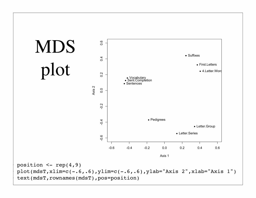
MDS plot

-0.6 -0.4 -0.2 0.0 0.2 0.4 0.6

-0.6

-0.4

-0.2

0.0

0.2

0.4

0.6

Axis 1

Axis

2

Sentences

VocabularySent.Completion

First.Letters

4.Letter.Words

Suffixes

Letter.Series

Pedigrees

Letter.Group

> position <- rep(4,9)> plot(mdsT,xlim=c(-.6,.6),ylim=c(-.6,.6),ylab="Axis 2",xlab="Axis 1")> text(mdsT,rownames(mdsT),pos=position)

A more complex example

I. Holzinger-Harman 24 mental ability tests

II. Compare FA, CA, MDS

Parallel analysis

5 10 15 20

02

46

8

Parallel Analysis Scree Plots

Factor Number

eig

en

va

lue

s o

f p

rin

cip

al co

mp

on

en

ts a

nd

fa

cto

r a

na

lysis

PC Actual Data

PC Simulated Data

FA Actual Data

FA Simulated Data

> hh <- Harman74.cor$cov> fa.parallel(hh,n.obs=228)

VSS says 1 big factor

1

1

1

11 1 1 1

1 2 3 4 5 6 7 8

0.0

0.2

0.4

0.6

0.8

1.0

Number of Factors

Very

Sim

ple

Str

uctu

re F

it


2

2

22 2 2

2

3 3 33 3

3

4 4 4 4 4

> vss <- VSS(hh,n.obs=228)

MAP suggests 4> vss

Very Simple StructureCall: VSS(x = hh, n.obs = 228)VSS complexity 1 achieves a maximimum of 0.8 with 1 factorsVSS complexity 2 achieves a maximimum of 0.85 with 2 factors

The Velicer MAP criterion achieves a minimum of 0.03 with 4 factors Velicer MAP[1] 0.02 0.02 0.02 0.02 0.02 0.02 0.03 0.03



Chi square says > 8

> vss$vss.stats[,1:3] dof chisq prob1 252 1012.9000 9.259262e-922 229 693.9911 2.649458e-483 207 485.1213 2.232607e-244 186 370.8825 2.174718e-145 166 307.7273 1.479600e-106 147 266.8324 5.628353e-097 129 226.6602 2.396296e-078 112 182.6407 2.832707e-05>

4 oblique factors

> fa4o <- factor.pa(hh,4,n.obs=228,rotate="oblimin")> fa4o V PA1 PA3 PA2 PA4VisualPerception 1 0.69 Cubes 2 0.46 PaperFormBoard 3 0.54 Flags 4 0.52 GeneralInformation 5 0.76 PargraphComprehension 6 0.80 SentenceCompletion 7 0.87 WordClassification 8 0.56 WordMeaning 9 0.86 Addition 10 0.86 Code 11 0.49 0.30CountingDots 12 0.70 StraightCurvedCapitals 13 0.42 0.47 WordRecognition 14 0.58NumberRecognition 15 0.55FigureRecognition 16 0.33 0.52ObjectNumber 17 0.59NumberFigure 18 0.43FigureWord 19 0.32Deduction 20 0.33 0.31 NumericalPuzzles 21 0.37 0.33 ProblemReasoning 22 0.31 0.30 SeriesCompletion 23 0.30 0.44 ArithmeticProblems 24 0.41

PA1 PA3 PA2 PA4SS loadings 3.52 2.29 2.14 1.80Proportion Var 0.15 0.10 0.09 0.08Cumulative Var 0.15 0.24 0.33 0.41

With factor correlations of PA1 PA3 PA2 PA4PA1 1.00 0.41 0.30 0.40PA3 0.41 1.00 0.27 0.38PA2 0.30 0.27 1.00 0.32

4 minres factors

4 oblique factors of the Holzinger-Harman problem

SentenceCompletionWordMeaning

PargraphComprehensionGeneralInformationWordClassification

DeductionProblemReasoningVisualPerceptionPaperFormBoard

FlagsCubes

SeriesCompletionNumericalPuzzles

AdditionCountingDots

CodeStraightCurvedCapitalsArithmeticProblemsObjectNumberWordRecognitionNumberRecognitionFigureRecognitionNumberFigureFigureWord

MR1

0.90.90.80.80.60.30.3

MR30.70.60.50.40.40.4

MR20.90.70.5 0.40.4

MR40.60.60.50.50.40.3

0.4

0.4

0.4

0.3

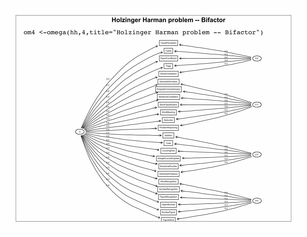
Holzinger Harman problem -- Bifactor

VisualPerception

Cubes

PaperFormBoard

Flags

GeneralInformation

PargraphComprehension

SentenceCompletion

WordClassification

WordMeaning

Addition

Code

CountingDots

StraightCurvedCapitals

WordRecognition

NumberRecognition

FigureRecognition

ObjectNumber

NumberFigure

FigureWord

Deduction

NumericalPuzzles

ProblemReasoning

SeriesCompletion

ArithmeticProblems

g

F1*

F2*

F3*

F4*

0.5

0.3

0.4

0.4

0.6

0.6

0.5

0.5

0.6

0.4

0.5

0.4

0.5

0.4

0.4

0.5

0.4

0.4

0.4

0.5

0.5

0.5

0.6

0.5

0.6

0.6

0.6

0.4

0.6

0.2

0.2

0.6

0.3

0.4

0.4

0.3

0.8

0.4

0.6

0.4

0.3

0.4

0.4

0.4

0.4

0.4

0.3

0.3

om4 <-omega(hh,4,title="Holzinger Harman problem -- Bifactor")

Holzinger Harman problem -- Hierarchical

VisualPerception

Cubes

PaperFormBoard

Flags

GeneralInformation


SentenceCompletion

WordClassification

WordMeaning

Addition

Code

CountingDots


WordRecognition

NumberRecognition

FigureRecognition

ObjectNumber

NumberFigure

FigureWord

Deduction

NumericalPuzzles

ProblemReasoning

SeriesCompletion

ArithmeticProblems

g

F1

F2

F3

F4

0.6

0.6

0.5

0.6

0.8

0.8

0.9

0.6

0.9

0.3

0.3

0.7

0.4

0.6

0.5

0.4

0.4

0.4

0.9

0.5

0.7

0.4

0.6

0.5

0.5

0.6

0.4

0.3

> om4 <-omega(hh,4,title="Holzinger Harman problem -- Hierarchical",sl=FALSE)

ICLUST of HHICLUST of Holzinger Harman 24 mental measurements

VisualPerception

Cubes

PaperFormBoard

Flags

GeneralInformation


SentenceCompletion

WordClassification

WordMeaning

Addition

Code

CountingDots


WordRecognition

NumberRecognition

FigureRecognition

ObjectNumber

NumberFigure

FigureWord

Deduction

NumericalPuzzles

ProblemReasoning

SeriesCompletion

ArithmeticProblems

C1

C2

C3

C4

C5

C6

C7

C8

C9

C10

C11 C12

C13

C14

C15

C16

C17

C18

C19

C20

C21

C22

C23

0.710.71

0.850.85

0.850.85

0.760.76

0.730.73

0.670.67

0.690.69

0.660.66

0.94

0.94

0.88

0.86

0.710.71

0.88

0.85

0.82

0.95

0.75

0.8

0.87

0.86

0.640.64

0.8

0.79

0.89

0.85

0.75

0.81

0.82

0.82

0.9

0.84

0.82

0.92

0.73

0.94

ic4 <- ICLUST(hh,title="ICLUST of Holzinger Harman 24 mental measurements")

Hierarchical cluster

analysis

ICLUST of Holzinger-Harman problem

C23! = 0.91! = 0.63

C22! = 0.91! = 0.76

0.65

C21! = 0.9! = 0.86

0.78

C20! = 0.86! = 0.74

0.94

C19! = 0.74! = 0.65

0.83

C17! = 0.64! = 0.58

0.82

FigureWord 0.7

C30.83NumberFigure 0.67

ObjectNumber 0.67

C14! = 0.64! = 0.6

0.82C80.71

FigureRecognition 0.66WordRecognition 0.66

NumberRecognition 0.71

C18! = 0.82! = 0.72

0.77

C12! = 0.79! = 0.74

0.73

C110.91

ArithmeticProblems 0.73NumericalPuzzles 0.73

C10! = 0.74! = 0.73

0.87C40.83

SeriesCompletion 0.71Deduction 0.71

ProblemReasoning 0.8

C16! = 0.66! = 0.6

0.85C70.67

Flags 0.68VisualPerception 0.68

PaperFormBoard 0.71

C13! = 0.9! = 0.79

0.68C9

! = 0.9! = 0.87

0.81

C10.95

WordMeaning 0.85GeneralInformation 0.85

C60.95SentenceCompletion 0.85

PargraphComprehension 0.85

WordClassification 0.83

C15! = 0.79! = 0.74

0.66C50.89

StraightCurvedCapitals 0.73Code 0.73

C20.85CountingDots 0.76

Addition 0.76

Cubes 0.6

MDS of HH problem

-0.6 -0.4 -0.2 0.0 0.2 0.4 0.6

-0.6

-0.4

-0.2

0.0

0.2

0.4

0.6

Dimension 1

Dim

en

sio

n 2

VisualPerception

Cubes

PaperFormBoard

Flags

GeneralInformation


SentenceCompletion

WordClassification

WordMeaning

Addition

Code

CountingDots


WordRecognition

NumberRecognition

FigureRecognition

ObjectNumber

NumberFigure

FigureWord

Deduction

NumericalPuzzles

ProblemReasoningSeriesCompletion

ArithmeticProblems

Multidimensional Scaling of 24 ability tests

code for MDS plot> dis24 <- sqrt(2*(1-Harman74.cor$cov))> mds24 <- cmdscale(dis24,2)> plot.char <- c( 19, 19, 19, 19, 21, 21, 21, 21, 21, 20, 20, 20, + 20, 23, 23, 23, 23, 23, 23, 19, 22, 19, 19, 22 )> plot(mds24,xlim=c(-.6,.6),ylim=c(-.6,.6),xlab="Dimension 1",ylab="Dimension 2",asp=1,pch=plot.char)> position <- c(2,2,3,4, 4,4,3,4, 3,2,3,2, 3,3,1,4, 4,1,3,1, 1,2,3,4)> text(mds24,rownames(mds24),cex=.6,pos=position)> abline(v=0,h=0)> title("Multidimensional Scaling of 24 ability tests")> #draw circles at .25 and .50 units away from the center> segments = 51 > angles <- (0:segments) * 2 * pi/segments> unit.circle <- cbind(cos(angles), sin(angles))> lines(unit.circle*.25)> lines(unit.circle*.5)

Reliability of scales and raters

I. First consider the reliability of raters using the IntraClass Correlation (see Shrout and Fleiss for the definitive discussion)

II. Types of reliability of ratings (1 or n per target)

A.each target rated by a different judge, judges are random

B. random sample of k judges rate targets

C. Fixed set of k judges give ratings

4 judges rate 6 subjects

> sf J1 J2 J3 J4S1 9 2 5 8S2 6 1 3 2S3 8 4 6 8S4 7 1 2 6S5 10 5 6 9S6 6 2 4 7

1

1

1

1

1

1

1 2 3 4 5 6

24

68

10

sf

2

2

2

2

2

2

3

3

3

3

3

3

4

4

4

4

4

4

Simple correlations (these will remove means for raters)> round(cor(sf),2) J1 J2 J3 J4J1 1.00 0.75 0.73 0.75J2 0.75 1.00 0.89 0.73J3 0.73 0.89 1.00 0.72J4 0.75 0.73 0.72 1.00

ICC> ICC(sf) type ICC F df1 df2 p lower bound upper boundSingle_raters_absolute ICC1 0.17 1.79 5 18 0.16 -0.13 0.72Single_random_raters ICC2 0.29 11.03 5 15 0.00 0.02 0.76Single_fixed_raters ICC3 0.71 11.03 5 15 0.00 0.34 0.95Average_raters_absolute ICC1k 0.44 1.79 5 18 0.16 -0.88 0.91Average_random_raters ICC2k 0.62 11.03 5 15 0.00 0.07 0.93Average_fixed_raters ICC3k 0.91 11.03 5 15 0.00 0.68 0.99

> alpha(sf)

Reliability analysis Call: alpha(x = sf)

raw_alpha std.alpha G6(smc) average_r mean sd 0.91 0.93 0.92 0.76 21 6.7

Reliability if an item is dropped: raw_alpha std.alpha G6(smc) average_rJ1 0.88 0.91 0.89 0.78J2 0.87 0.89 0.85 0.73J3 0.87 0.90 0.85 0.74J4 0.92 0.92 0.90 0.79

Alpha of raters

Item statistics n r r.cor mean sdJ1 6 0.89 0.83 7.7 1.6J2 6 0.93 0.92 2.5 1.6J3 6 0.92 0.91 4.3 1.6J4 6 0.88 0.82 6.7 2.5

Reliability of a single scale

> round(cor(bfi[,1:10],use="pairwise"),2) A1 A2 A3 A4 A5 C1 C2 C3 C4 C5A1 1.00 -0.30 -0.23 -0.12 -0.19 -0.03 -0.06 0.01 0.19 0.08A2 -0.30 1.00 0.39 0.24 0.41 0.06 0.06 0.22 -0.15 -0.12A3 -0.23 0.39 1.00 0.27 0.45 0.07 0.12 0.16 -0.14 -0.12A4 -0.12 0.24 0.27 1.00 0.22 0.07 0.17 0.08 -0.15 -0.17A5 -0.19 0.41 0.45 0.22 1.00 0.10 0.06 0.20 -0.14 -0.10C1 -0.03 0.06 0.07 0.07 0.10 1.00 0.44 0.41 -0.39 -0.23C2 -0.06 0.06 0.12 0.17 0.06 0.44 1.00 0.35 -0.36 -0.24C3 0.01 0.22 0.16 0.08 0.20 0.41 0.35 1.00 -0.37 -0.36C4 0.19 -0.15 -0.14 -0.15 -0.14 -0.39 -0.36 -0.37 1.00 0.53C5 0.08 -0.12 -0.12 -0.17 -0.10 -0.23 -0.24 -0.36 0.53 1.00

Mindless reliability> alpha(bfi[1:10])

Reliability analysis Call: alpha(x = bfi[1:10])


Reliability if an item is dropped: raw_alpha std.alpha G6(smc) average_rA1 0.290 0.354 0.51 0.057A2 0.082 0.133 0.35 0.017A3 0.045 0.101 0.33 0.012A4 0.108 0.173 0.40 0.023A5 0.042 0.093 0.32 0.011C1 0.133 0.190 0.38 0.025C2 0.123 0.182 0.38 0.024C3 0.105 0.154 0.36 0.020C4 0.336 0.392 0.50 0.067C5 0.329 0.364 0.49 0.060

Item statistics n r r.cor mean sdA1 1000 0.099 -0.21 2.3 1.3A2 994 0.508 0.47 4.8 1.1A3 989 0.552 0.54 4.6 1.2A4 993 0.448 0.31 4.8 1.4A5 988 0.563 0.55 4.6 1.2C1 997 0.421 0.34 4.4 1.2C2 997 0.434 0.35 4.2 1.3C3 995 0.478 0.44 4.3 1.3C4 986 0.005 -0.24 2.6 1.4C5 997 0.077 -0.17 3.5 1.5

somewhat better reliability> keys <- make.keys(10,list(all=c(-1,2:8,-9,-10)))> alpha(bfi[1:10],keys)

Reliability analysis Call: alpha(x = bfi[1:10], keys = keys)


Reliability if an item is dropped: raw_alpha std.alpha G6(smc) average_rA1 0.72 0.72 0.74 0.23A2 0.70 0.70 0.72 0.20A3 0.70 0.70 0.72 0.20A4 0.71 0.71 0.74 0.22A5 0.70 0.70 0.72 0.21C1 0.70 0.70 0.72 0.21C2 0.70 0.70 0.72 0.21C3 0.69 0.69 0.71 0.20C4 0.67 0.68 0.70 0.19C5 0.70 0.70 0.72 0.20

Item statistics n r r.cor mean sdA1 1000 0.41 0.29 2.3 1.3A2 994 0.55 0.49 4.8 1.1A3 989 0.55 0.49 4.6 1.2A4 993 0.46 0.35 4.8 1.4A5 988 0.53 0.46 4.6 1.2C1 997 0.52 0.46 4.4 1.2C2 997 0.54 0.47 4.2 1.3C3 995 0.59 0.54 4.3 1.3C4 986 0.64 0.61 2.6 1.4C5 997 0.55 0.49 3.5 1.5

Examine the items

A1Am indifferent to the feelings of others.A2Inquire about others' well-being.A3Know how to comfort others.A4Love children.A5Make people feel at ease.C1Am exacting in my work.C2Continue until everything is perfect.C3Do things according to a plan.C4Do things in a half-way manner.C5Waste my time.

The items

1

1

11

1 1

11

1 2 3 4 5 6 7 8

0.0

0.2

0.4

0.6

0.8

1.0

Number of Factors

Ve

ry S

imp

le S

tru

ctu

re F

it


22 2

2 22 2

33

3 3 33

4

44

44

VSS suggests 2 factors!

Omega reliability

> om2 <- omega(bfi[1:10],2)Warning messages:1: In schmid(m, nfactors, pc, digits, rotate = rotate, n.obs = n.obs, : Three factors are required for identification -- general factor loadings set to be equal. Proceed with caution.2: In schmid(m, nfactors, pc, digits = digits, n.obs = n.obs, ...) : Three factors are required for identification -- general factor loadings set to be equal. Proceed with caution.

Omega h is low

> om2Omega Call: omega(m = bfi[1:10], nfactors = 2)Alpha: 0.72 G.6: 0.75 Omega Hierarchical: 0.36 Omega Total 0.77

Schmid Leiman Factor loadings greater than 0.2 g F1* F2* h2 u2 A1- 0.21 0.30 0.87A2 0.36 0.53 0.41 0.59A3 0.36 0.55 0.43 0.57A4 0.24 0.28 0.86A5 0.36 0.54 0.42 0.58C1 0.30 0.51 0.36 0.64C2 0.30 0.48 0.32 0.68C3 0.37 0.48 0.37 0.63C4- 0.40 0.58 0.50 0.50C5- 0.33 0.48 0.33 0.67

With eigenvalues of: g F1* F2* 1.1 1.3 1.1

Score 3 scales

> keys <- make.keys(10,list(all=c(-1,2:8,-9,-10),agree=c(-1,2:5),con=c(6:8,-9,-10)))> score.items(keys,bfi[1:10])Call: score.items(keys = keys, items = bfi[1:10])

(Unstandardized) Alpha: all agree conalpha 0.72 0.65 0.74

Average item correlation: all agree conaverage.r 0.2 0.27 0.36

Guttman 6* reliability: all agree conLambda.6 0.74 0.62 0.72

Scale intercorrelations corrected for attenuation raw correlations below the diagonal, alpha on the diagonal corrected correlations above the diagonal: all agree conall 0.72 1.10 1.13agree 0.75 0.65 0.36con 0.83 0.25 0.74

Item scale correlations

Item by scale correlations: corrected for item overlap and scale reliability all agree conA1 -0.28 -0.37 -0.12A2 0.47 0.63 0.21A3 0.47 0.63 0.21A4 0.34 0.37 0.22A5 0.44 0.58 0.20C1 0.46 0.13 0.59C2 0.47 0.19 0.55C3 0.54 0.25 0.60C4 -0.62 -0.30 -0.69C5 -0.50 -0.23 -0.56>

ICLUST shows 2 scalesICLUST

A1

A2

A3

A4

A5

C1

C2

C3

C4

C5

C1

C2

C3

C4

C5

C6

C7C8

0.660.66

0.730.73

0.670.67

0.810.83

0.780.82

0.80.83

0.660.82

-0.61-0.82

Structural Equation modeling in R

I. sem by John Fox

II. does not do multiple group analyses

III.Mx in R is a coming attraction

IV.Using psych as a front end to sem to generate the model commands

Using psych as front end to sem

I. Do the exploratory analysis (fa or omega) in psych

II. output includes the sem model instructions

III.run sem

IV.(see the vignette on using psych for sem)

The model

> om <- omega(Thurstone) #creates the path model and the model commands> om$model Path Parameter Initial Value [1,] "g->Sentences" "Sentences" NA [2,] "g->Vocabulary" "Vocabulary" NA [3,] "g->Sent.Completion" "Sent.Completion" NA [4,] "g->First.Letters" "First.Letters" NA [5,] "g->4.Letter.Words" "4.Letter.Words" NA [6,] "g->Suffixes" "Suffixes" NA [7,] "g->Letter.Series" "Letter.Series" NA [8,] "g->Pedigrees" "Pedigrees" NA [9,] "g->Letter.Group" "Letter.Group" NA [10,] "F1*->Sentences" "F1*Sentences" NA [11,] "F1*->Vocabulary" "F1*Vocabulary" NA [12,] "F1*->Sent.Completion" "F1*Sent.Completion" NA [13,] "F2*->First.Letters" "F2*First.Letters" NA [14,] "F2*->4.Letter.Words" "F2*4.Letter.Words" NA [15,] "F2*->Suffixes" "F2*Suffixes" NA [16,] "F3*->Letter.Series" "F3*Letter.Series" NA [17,] "F3*->Pedigrees" "F3*Pedigrees" NA [18,] "F3*->Letter.Group" "F3*Letter.Group" NA [19,] "Sentences<->Sentences" "e1" NA [20,] "Vocabulary<->Vocabulary" "e2" NA [21,] "Sent.Completion<->Sent.Completion" "e3" NA [22,] "First.Letters<->First.Letters" "e4" NA [23,] "4.Letter.Words<->4.Letter.Words" "e5" NA [24,] "Suffixes<->Suffixes" "e6" NA [25,] "Letter.Series<->Letter.Series" "e7" NA [26,] "Pedigrees<->Pedigrees" "e8" NA [27,] "Letter.Group<->Letter.Group" "e9" NA [28,] "F1*<->F1*" NA "1" [29,] "F2*<->F2*" NA "1" [30,] "F3*<->F3*" NA "1" [31,] "g <->g" NA "1" >

The modelOmega

Sentences

Vocabulary

Sent.Completion

First.Letters

4.Letter.Words

Suffixes

Letter.Series

Pedigrees

Letter.Group

g

F1*

F2*

F3*

0.7

0.7

0.7

0.6

0.6

0.6

0.6

0.6

0.5

0.6

0.6

0.5

0.6

0.5

0.4

0.6

0.3

0.5

Do the sem> library(sem)> sem.bf <- sem(om$model,Thurstone,213)> summary(sem.bf,digits=2)

Model Chisquare = 24 Df = 18 Pr(>Chisq) = 0.15 Chisquare (null model) = 1102 Df = 36 Goodness-of-fit index = 0.98 Adjusted goodness-of-fit index = 0.94 RMSEA index = 0.04 90% CI: (NA, 0.078) Bentler-Bonnett NFI = 0.98 Tucker-Lewis NNFI = 0.99 Bentler CFI = 1 SRMR = 0.035 BIC = -72

Normalized Residuals Min. 1st Qu. Median Mean 3rd Qu. Max. -8.2e-01 -3.3e-01 -8.9e-07 2.8e-02 1.6e-01 1.8e+00

Parameter values Parameter Estimates Estimate Std Error z value Pr(>|z|) Sentences 0.77 0.073 10.57 0.0e+00 Sentences <--- g Vocabulary 0.79 0.072 10.92 0.0e+00 Vocabulary <--- g Sent.Completion 0.75 0.073 10.27 0.0e+00 Sent.Completion <--- g First.Letters 0.61 0.072 8.43 0.0e+00 First.Letters <--- g 4.Letter.Words 0.60 0.074 8.09 6.7e-16 4.Letter.Words <--- g Suffixes 0.57 0.071 8.00 1.3e-15 Suffixes <--- g Letter.Series 0.57 0.074 7.63 2.3e-14 Letter.Series <--- g Pedigrees 0.66 0.069 9.55 0.0e+00 Pedigrees <--- g Letter.Group 0.53 0.079 6.71 2.0e-11 Letter.Group <--- g F1*Sentences 0.49 0.085 5.71 1.1e-08 Sentences <--- F1* F1*Vocabulary 0.45 0.090 5.00 5.7e-07 Vocabulary <--- F1* F1*Sent.Completion 0.40 0.093 4.33 1.5e-05 Sent.Completion <--- F1* F2*First.Letters 0.61 0.086 7.16 8.2e-13 First.Letters <--- F2* F2*4.Letter.Words 0.51 0.085 5.96 2.5e-09 4.Letter.Words <--- F2* F2*Suffixes 0.39 0.078 5.04 4.7e-07 Suffixes <--- F2* F3*Letter.Series 0.73 0.159 4.56 5.1e-06 Letter.Series <--- F3* F3*Pedigrees 0.25 0.089 2.77 5.6e-03 Pedigrees <--- F3* F3*Letter.Group 0.41 0.122 3.35 8.1e-04 Letter.Group <--- F3* e1 0.17 0.034 5.05 4.4e-07 Sentences <--> Sentences e2 0.17 0.030 5.65 1.6e-08 Vocabulary <--> Vocabulary e3 0.27 0.033 8.09 6.7e-16 Sent.Completion <-->Sent.Compe4 0.25 0.079 3.18 1.5e-03 First.Letters <-First.Letters e5 0.39 0.063 6.13 8.8e-10 4.Letter.Words <-->4.Letter.Words e6 0.52 0.060 8.68 0.0e+00 Suffixes <--> Suffixes e7 0.15 0.223 0.67 5.0e-01 Letter.Series <--> Letter.Series e8 0.50 0.060 8.39 0.0e+00 Pedigrees <--> Pedigrees e9 0.55 0.085 6.51 7.4e-11 Letter.Group <--> Letter.Group

Programming in RI. Very high level language

A.interpreted at run time

B. can integrate Fortran or C++ code

II. 3 ways of developing code

A.cut and paste from an editor

B. Modify prior code by adding or changing a function

C. source from a file

D.build a package for local or global distribution

Programming in RI. functions and data structures

A.The output of all functions is an object that will have a certain structure

B. Part of the structure might be invisible but can be shown with the str() command.

1. f3 <- fa(Thurstone,3,rotate=oblimin)

2. str(f3) #will show more than just asking for f3

selected output> f3 <- fa(Thurstone,3,rotate="oblimin")> f3Factor Analysis using method = minresCall: fa(r = Thurstone, nfactors = 3, rotate = "oblimin") item MR1 MR2 MR3 h2 u2Sentences 1 0.90 0.82 0.18Vocabulary 2 0.89 0.84 0.16Sent.Completion 3 0.84 0.74 0.26First.Letters 4 0.85 0.73 0.274.Letter.Words 5 0.75 0.63 0.37Suffixes 6 0.63 0.50 0.50Letter.Series 7 0.84 0.72 0.28Pedigrees 8 0.38 0.47 0.50 0.50Letter.Group 9 0.63 0.52 0.48 MR1 MR2 MR3SS loadings 2.64 1.87 1.49Proportion Var 0.29 0.21 0.17Cumulative Var 0.29 0.50 0.67 With factor correlations of MR1 MR2 MR3MR1 1.00 0.59 0.53MR2 0.59 1.00 0.52MR3 0.53 0.52 1.00Test of the hypothesis that 3 factors are sufficient.The degrees of freedom for the model is 12 and the objective function was 0.01 Fit based upon off diagonal values = 1Measures of factor score adequacy [,1] [,2] [,3]Correlation of scores with factors 0.96 0.92 0.90Multiple R square of scores with factors 0.93 0.85 0.82Minimum correlation of factor score estimates 0.86 0.71 0.63

All the output (too much)> print(f3,all=TRUE)Factor Analysis using method = minresCall: fa(r = Thurstone, nfactors = 3, rotate = "oblimin") item MR1 MR2 MR3 h2 u2Sentences 1 0.90 0.82 0.18Vocabulary 2 0.89 0.84 0.16Sent.Completion 3 0.84 0.74 0.26First.Letters 4 0.85 0.73 0.274.Letter.Words 5 0.75 0.63 0.37Suffixes 6 0.63 0.50 0.50Letter.Series 7 0.84 0.72 0.28Pedigrees 8 0.38 0.47 0.50 0.50Letter.Group 9 0.63 0.52 0.48


With factor correlations of MR1 MR2 MR3MR1 1.00 0.59 0.53MR2 0.59 1.00 0.52MR3 0.53 0.52 1.00


The degrees of freedom for the model is 12 and the objective function was 0.01

Fit based upon off diagonal values = 1Measures of factor score adequacy [,1] [,2] [,3]Correlation of scores with factors 0.96 0.92 0.90Multiple R square of scores with factors 0.93 0.85 0.82Minimum correlation of factor score estimates 0.86 0.71 0.63$residual Sentences Vocabulary Sent.Completion First.Letters 4.Letter.WordsSentences 0.1797970835 0.003569352 0.001056412 -0.0053521359 0.0054931042Vocabulary 0.0035693518 0.164376546 -0.004726931 0.0015287573 -0.0013163850Sent.Completion 0.0010564117 -0.004726931 0.264475270 0.0064257822 -0.0061643080First.Letters -0.0053521359 0.001528757 0.006425782 0.2708794227 -0.00074622374.Letter.Words 0.0054931042 -0.001316385 -0.006164308 -0.0007462237 0.3691635597Suffixes -0.0005413284 0.003307528 -0.006202623 0.0009046706 -0.0007702702Letter.Series -0.0001193089 0.005601586 -0.009592364 0.0036158583 -0.0048190635Pedigrees -0.0103409056 -0.003359723 0.020557454 -0.0045780810 0.0019664267Letter.Group 0.0074095333 -0.010637633 0.007277838 -0.0037248900 0.0083593427 Suffixes Letter.Series Pedigrees Letter.GroupSentences -0.0005413284 -0.0001193089 -0.010340906 0.0074095333Vocabulary 0.0033075284 0.0056015857 -0.003359723 -0.0106376334Sent.Completion -0.0062026235 -0.0095923640 0.020557454 0.0072778382First.Letters 0.0009046706 0.0036158583 -0.004578081 -0.00372489004.Letter.Words -0.0007702702 -0.0048190635 0.001966427 0.0083593427Suffixes 0.5040410452 -0.0014514317 0.006481298 -0.0007367270Letter.Series -0.0014514317 0.2750324849 0.001571784 -0.0008933238Pedigrees 0.0064812977 0.0015717836 0.496000068 -0.0025752061Letter.Group -0.0007367270 -0.0008933238 -0.002575206 0.4760216108

$score.cor [,1] [,2] [,3][1,] 1.0000000 0.5711316 0.5744068[2,] 0.5711316 1.0000000 0.5155396[3,] 0.5744068 0.5155396 1.0000000

$weights [,1] [,2] [,3]Sentences 0.353322510 -0.009407414 0.050820832Vocabulary 0.385959584 0.075436552 -0.015772944Sent.Completion 0.228403072 0.033052383 0.006244325First.Letters 0.010855524 0.464020963 0.0195776214.Letter.Words 0.005034161 0.300298831 0.061015049Suffixes 0.029796749 0.183531257 -0.023285274Letter.Series 0.013748571 0.008558551 0.564027583Pedigrees 0.055852379 -0.007387944 0.174505325Letter.Group -0.005072886 0.071298123 0.245089238

$communality Sentences Vocabulary Sent.Completion First.Letters 4.Letter.Words 0.82 0.84 0.74 0.73 0.63 Suffixes Letter.Series Pedigrees Letter.Group 0.50 0.72 0.50 0.52

$uniquenesses Sentences Vocabulary Sent.Completion First.Letters 4.Letter.Words 0.18 0.16 0.26 0.27 0.37 Suffixes Letter.Series Pedigrees Letter.Group 0.50 0.28 0.50 0.48

$values[1] 4.85 1.09 1.04 0.48 0.45 0.37 0.32 0.23 0.17

$loadings

Loadings: MR1 MR2 MR3 Sentences 0.904 Vocabulary 0.889 Sent.Completion 0.835 First.Letters 0.853 4.Letter.Words 0.747 0.101Suffixes 0.180 0.627 Letter.Series 0.842Pedigrees 0.377 0.467Letter.Group 0.210 0.630


$fm[1] "minres"

$Phi [,1] [,2] [,3][1,] 1.0000000 0.5922606 0.5349450[2,] 0.5922606 1.0000000 0.5168493[3,] 0.5349450 0.5168493 1.0000000

$fn[1] "fa"

>

$fit[1] 0.9569096

$fit.off[1] 0.9998501

$factors[1] 3

$n.obs[1] NA

$PVAL[1] NA

$dof[1] 12

$objective[1] 0.01390055

$criteria objective 0.01390055 NA NA

$Callfa(r = Thurstone, nfactors = 3, rotate = "oblimin")

$r.scores [,1] [,2] [,3][1,] 1.0000000 0.6615062 0.6122765[2,] 0.6615062 1.0000000 0.6134362[3,] 0.6122765 0.6134362 1.0000000

$R2[1] 0.9285797 0.8525374 0.8161127

$valid[1] 0.9598034 0.9078568 0.8823116

Using str to show

what is there

> f3 <- fa(Thurstone,3,rotate="oblimin")> str(f3)List of 22 $ residual : num [1:9, 1:9] 0.1798 0.00357 0.00106 -0.00535 0.00549 ... ..- attr(*, "dimnames")=List of 2 .. ..$ : chr [1:9] "Sentences" "Vocabulary" "Sent.Completion" "First.Letters" ... .. ..$ : chr [1:9] "Sentences" "Vocabulary" "Sent.Completion" "First.Letters" ... $ fit : num 0.957 $ fit.off : num 1 $ factors : num 3 $ n.obs : logi NA $ PVAL : logi NA $ dof : num 12 $ objective : num 0.0139 $ criteria : Named num [1:3] 0.0139 NA NA ..- attr(*, "names")= chr [1:3] "objective" "" "" $ Call : language fa(r = Thurstone, nfactors = 3, rotate = "oblimin") $ r.scores : num [1:3, 1:3] 1 0.662 0.612 0.662 1 ... $ R2 : num [1:3] 0.929 0.853 0.816 $ valid : num [1:3] 0.96 0.908 0.882 $ score.cor : num [1:3, 1:3] 1 0.571 0.574 0.571 1 ... $ weights : num [1:9, 1:3] 0.35332 0.38596 0.2284 0.01086 0.00503 ... ..- attr(*, "dimnames")=List of 2 .. ..$ : chr [1:9] "Sentences" "Vocabulary" "Sent.Completion" "First.Letters" ... .. ..$ : NULL $ communality : Named num [1:9] 0.82 0.84 0.74 0.73 0.63 0.5 0.72 0.5 0.52 ..- attr(*, "names")= chr [1:9] "Sentences" "Vocabulary" "Sent.Completion" "First.Letters" ... $ uniquenesses: Named num [1:9] 0.18 0.16 0.26 0.27 0.37 0.5 0.28 0.5 0.48 ..- attr(*, "names")= chr [1:9] "Sentences" "Vocabulary" "Sent.Completion" "First.Letters" ... $ values : num [1:9] 4.85 1.09 1.04 0.48 0.45 0.37 0.32 0.23 0.17 $ loadings : loadings [1:9, 1:3] 0.90356 0.889 0.83522 -0.00297 -0.01535 ... ..- attr(*, "dimnames")=List of 2 .. ..$ : chr [1:9] "Sentences" "Vocabulary" "Sent.Completion" "First.Letters" ... .. ..$ : chr [1:3] "MR1" "MR2" "MR3" $ fm : chr "minres" $ Phi : num [1:3, 1:3] 1 0.592 0.535 0.592 1 ... $ fn : chr "fa" - attr(*, "class")= chr [1:2] "psych" "fa"

Programming in R

I. Data types

II. operators

III. simple functions

IV.Writing functions

Data structuresI. elements: logical, integer, real, character, factor

II. vectors: ordered sets of elements of one type

III.matrices: ordered sets of vectors (all of one type)

IV. data.frames: ordered sets of vectors, may be different types

V.lists: ordered set of anything

OperatorsI. arithmetical

1. +, -, *, /, ^, %%

2. a + b, a-b, a*b, a/b, a^b, a %%b

II. Logical

A.a==b, !a, a!=b, a>b, a<b, a>=b,a <=b

III.Matrix

A.%*% is matrix multiplication

B. %o% is outer product

example operations> a <- 2> b <- 3> v <- 5:10> w <- 6:7> v[1] 5 6 7 8 9 10> w[1] 6 7> v ^a[1] 25 36 49 64 81 100> w* b[1] 18 21> w * v[1] 30 42 42 56 54 70

Matrix operations> v[1] 5 6 7 8 9 10> t(v) [,1] [,2] [,3] [,4] [,5] [,6][1,] 5 6 7 8 9 10> t(v)%*% v [,1][1,] 355> v %*% t(v) [,1] [,2] [,3] [,4] [,5] [,6][1,] 25 30 35 40 45 50[2,] 30 36 42 48 54 60[3,] 35 42 49 56 63 70[4,] 40 48 56 64 72 80[5,] 45 54 63 72 81 90[6,] 50 60 70 80 90 100

Additional matrix operators

> v[1] 5 6 7 8 9 10> w[1] 6 7> v %o% w [,1] [,2][1,] 30 35[2,] 36 42[3,] 42 49[4,] 48 56[5,] 54 63[6,] 60 70

outer product

> x <- seq(4,8,2)> x[1] 4 6 8

> x %+% t(x) [,1] [,2] [,3][1,] 8 10 12[2,] 10 12 14[3,] 12 14 16

matrix “addition” (psych)

kronecker

Functions

I. Operate on an object and provide a new object

II. e.g., f <- function(x) {x * 2}

Simple functions

> f <- function(x) {x * 2} > f(43)[1] 86> x[1] 4 6 8> f(x)[1] 8 12 16> f( v %o% w) [,1] [,2][1,] 60 70[2,] 72 84[3,] 84 98[4,] 96 112[5,] 108 126[6,] 120 140

a subset of useful functionsI. is.na(), is.null(), is.vector(), is.matrix(), is.list

()

II. sum(), rowSums(), colSums(), mean(x), rowMeans(), colMeans(), max, min, median (these work on the entire matrix)

III.var, cov, cor, sd (these work on the columns of the matrix/data.frame)

IV. help.start() brings up a web page of manuals

More useful functions

I. rep(x,n) (repeats the value x n times)

II. c(x,y) (combines x with y)

III.cbind(x,y) combines column wise

IV.rbind(x,y) combines rowwise

V.seq(a,b,c) sequence from a to b stepping by c

sums on matrices and data.frames> z <- f( v %o% w)

> z [,1] [,2][1,] 60 70[2,] 72 84[3,] 84 98[4,] 96 112[5,] 108 126[6,] 120 140

> sum(z)[1] 1170> min(z)[1] 60> max(z)[1] 140> median(z)[1] 97

> rowSums(z)[1] 130 156 182 208 234 260> colSums(z)[1] 540 630> mean(z)[1] 97.5> rowMeans(z)[1] 65 78 91 104 117 130

Basic stats functions,

part 2

> var(z) [,1] [,2][1,] 504 588[2,] 588 686> cov(z) [,1] [,2][1,] 504 588[2,] 588 686> cor(z) [,1] [,2][1,] 1 1[2,] 1 1> sd(z)[1] 22.44994 26.19160> z [,1] [,2][1,] 60 70[2,] 72 84[3,] 84 98[4,] 96 112[5,] 108 126[6,] 120 140

?cor var(x, y = NULL, na.rm = FALSE, use)

cov(x, y = NULL, use = "everything", method = c("pearson", "kendall", "spearman"))

cor(x, y = NULL, use = "everything", method = c("pearson", "kendall", "spearman"))

cov2cor(V)

More on corxa numeric vector, matrix or data frame.yNULL (default) or a vector, matrix or data frame with compatible dimensions to x. The default is equivalent to y = x (but more efficient).na.rmlogical. Should missing values be removed?usean optional character string giving a method for computing covariances in the presence of missing values. This must be (an abbreviation of) one of the strings "everything", "all.obs", "complete.obs", "na.or.complete", or "pairwise.complete.obs".methoda character string indicating which correlation coefficient (or covariance) is to be computed. One of "pearson" (default), "kendall", or "spearman", can be abbreviated.Vsymmetric numeric matrix, usually positive definite such as a covariance matrix.

row and col as functions

> r <- .8> R <- diag(1,8)> R [,1] [,2] [,3] [,4] [,5] [,6] [,7] [,8][1,] 1 0 0 0 0 0 0 0[2,] 0 1 0 0 0 0 0 0[3,] 0 0 1 0 0 0 0 0[4,] 0 0 0 1 0 0 0 0[5,] 0 0 0 0 1 0 0 0[6,] 0 0 0 0 0 1 0 0[7,] 0 0 0 0 0 0 1 0[8,] 0 0 0 0 0 0 0 1> R <- r^(abs(row(R)-col(R)))> round(R,2) [,1] [,2] [,3] [,4] [,5] [,6] [,7] [,8][1,] 1.00 0.80 0.64 0.51 0.41 0.33 0.26 0.21[2,] 0.80 1.00 0.80 0.64 0.51 0.41 0.33 0.26[3,] 0.64 0.80 1.00 0.80 0.64 0.51 0.41 0.33[4,] 0.51 0.64 0.80 1.00 0.80 0.64 0.51 0.41[5,] 0.41 0.51 0.64 0.80 1.00 0.80 0.64 0.51[6,] 0.33 0.41 0.51 0.64 0.80 1.00 0.80 0.64[7,] 0.26 0.33 0.41 0.51 0.64 0.80 1.00 0.80[8,] 0.21 0.26 0.33 0.41 0.51 0.64 0.80 1.00

Yet more stats functions

I. sample(n, N, replace=TRUE)

II. eigen(X) (eigen value decomposition of X)

III.solve(X) (inverse of X)

IV. solve (X,Y) Regression of Y on X

Creating a matrix

> x <- matrix(sample(10,50,replace=TRUE),ncol=5)> x [,1] [,2] [,3] [,4] [,5] [1,] 10 3 4 4 6 [2,] 3 10 8 8 9 [3,] 1 6 5 8 5 [4,] 9 1 3 5 3 [5,] 6 8 3 5 1 [6,] 8 6 10 1 10 [7,] 10 5 10 2 1 [8,] 9 3 2 2 9 [9,] 6 10 2 9 4[10,] 1 8 8 2 6

> z <- scale(x)> z [,1] [,2] [,3] [,4] [,5] [1,] 1.04838349 -0.9819805 -0.4678877 -0.2059329 0.1852621 [2,] -0.93504473 1.3093073 0.7798129 1.1669533 1.1115724 [3,] -1.50173851 0.0000000 -0.1559626 1.1669533 -0.1235080 ... [9,] -0.08500407 1.3093073 -1.0917380 1.5101749 -0.4322782[10,] -1.50173851 0.6546537 0.7798129 -0.8923761 0.1852621attr(,"scaled:center")[1] 6.3 6.0 5.5 4.6 5.4attr(,"scaled:scale")[1] 3.529243 3.055050 3.205897 2.913570 3.238655

standardize it

Just center it> c <- scale(x,scale=FALSE)

> c [,1] [,2] [,3] [,4] [,5] [1,] 3.7 -3 -1.5 -0.6 0.6 [2,] -3.3 4 2.5 3.4 3.6 [3,] -5.3 0 -0.5 3.4 -0.4 [4,] 2.7 -5 -2.5 0.4 -2.4 [5,] -0.3 2 -2.5 0.4 -4.4 [6,] 1.7 0 4.5 -3.6 4.6 [7,] 3.7 -1 4.5 -2.6 -4.4 [8,] 2.7 -3 -3.5 -2.6 3.6 [9,] -0.3 4 -3.5 4.4 -1.4[10,] -5.3 2 2.5 -2.6 0.6attr(,"scaled:center")[1] 6.3 6.0 5.5 4.6 5.4

Find the covariance and inverse

> c <- cov(x)> round(c,2) [,1] [,2] [,3] [,4] [,5][1,] 12.46 -6.89 -1.61 -4.53 -1.58[2,] -6.89 9.33 2.11 4.11 0.56[3,] -1.61 2.11 10.28 -3.89 2.22[4,] -4.53 4.11 -3.89 8.49 -1.60[5,] -1.58 0.56 2.22 -1.60 10.49

> round(solve(c),2) [,1] [,2] [,3] [,4] [,5][1,] 0.15 0.08 0.02 0.06 0.02[2,] 0.08 0.23 -0.07 -0.10 0.00[3,] 0.02 -0.07 0.16 0.12 -0.01[4,] 0.06 -0.10 0.12 0.26 0.03[5,] 0.02 0.00 -0.01 0.03 0.10

Flow control

I. if(condition) {then do this} else {do this}

II. for (condition) do {expression}

A.for (i in 1:n} do {x <- x + 1}

III.while (condition) {expression}

conditionalsI. (a & b) vs. (a && b)

II. (a | b) vs. (a || b)

a <- 1> if (a & b) {print ("hello")} else {print("goodby")}Error: object 'b' not found> if (a && b ) {print ("hello")} else {print("goodby")}[1] "goodby"> if (a | b) {print ("hello")} else {print("goodby")}Error: object 'b' not found > if (a || b) {print ("hello")} else {print("goodby")}Error: object 'b' not found> a <- 1> if (a || b) {print ("hello")} else {print("goodby")}[1] "hello">

simple control> a <- 1 > b <- 2> c <- 3> k <- 10> x <-1 > if(x == a) {print("x is the same as a and has value",x)} else {print ("x is not equal to a")}

> x <- 3> if(x == a) {print("x is the same as a and has value",x)} else {print ("x is not equal to a")}[1] "x is not equal to a">

Make that a function> f1 <- function(x,y) {if(x == y) {print("x is the same as y and has value",x)} else {print ("x is not equal to y")}}> f1(3,4)[1] "x is not equal to y"> f1(5,5)[1] "x is the same as y and has value"

Simple functions:part 2

I. Find the squared multiple correlation of a variable with all the other variables in a matrix.

II. The R2 is 1- the residual variance

The essence of the function

SMC <- function(R) {R.inv <- solve(R)SMC <- 1 - 1/diag(R.inv)}

> S <-cor(attitude)> SMC(S) #does not show anything

> round(SMC(S),2) #but this does rating complaints privileges learning raises critical advance 0.73 0.77 0.38 0.62 0.68 0.19 0.52

Add a return

SMC <- function(R) {R.inv <- solve(R)SMC <- 1 - 1/diag(R.inv)return(SMC)}

> SMC(S) rating complaints privileges learning raises critical advance 0.7326020 0.7700868 0.3831176 0.6194561 0.6770498 0.1881465 0.5186447

Allow it to find RSMC <- function(R) {if(dim(R)[1] !=dim(R)[2]) {R <-cor(R)}R.inv <- solve(R)SMC <- 1 - 1/diag(R.inv)return(SMC)}

> SMC(attitude) rating complaints privileges learning raises critical advance 0.7326020 0.7700868 0.3831176 0.6194561 0.6770498 0.1881465 0.5186447

Clean up the outputSMC <- function(R,digits=2) {if(dim(R)[1] !=dim(R)[2]) {R <-cor(R)}R.inv <- solve(R)SMC <- 1 - 1/diag(R.inv)return(round(SMC,digits))}

> SMC(attitude) rating complaints privileges learning raises critical advance 0.73 0.77 0.38 0.62 0.68 0.19 0.52 >

Check for poor input> att <- data.frame(attitude[1:3],attitude[1:3])> SMC(att)Error in solve.default(R) : Lapack routine dgesv: system is exactly singular

Add checks for weird matrices

SMC <- function(R,digits=2) { p <- dim(R)[2] if (dim(R)[1] != p) {R <-cor(R)}R.inv <- try(solve(R),TRUE)if(class(R.inv)== as.character("try-error")) {SMC <- rep(1,p) warning("Correlation matrix not invertible, smc's returned as 1s")} else {smc <- 1 -1/diag(R.inv)SMC <- 1 - 1/diag(R.inv)}return(round(SMC,digits))}

> SMC(att)[1] 1 1 1 1 1 1Warning message:In SMC(att) : Correlation matrix not invertible, smc's returned as 1s

> SMC(attitude) rating complaints privileges learning raises critical 0.73 0.77 0.38 0.62 0.68 0.19

Further checks Input is a covariance matrix > SMC(cov(attitude)) rating complaints privileges learning raises critical advance -38.62 -39.76 -91.35 -51.42 -33.91 -78.49 -49.96

> SMC(cor(attitude)) rating complaints privileges learning raises critical advance 0.73 0.77 0.38 0.62 0.68 0.19 0.52 > SMC(attitude) rating complaints privileges learning raises critical advance 0.73 0.77 0.38 0.62 0.68 0.19 0.52

Input is raw data or correlations

Final version#modified Dec 10, 2008 to return 1 on diagonal if non-invertible#modifed March 20, 2009 to return smcs * variance if covariance matrix is desired#modified April 8, 2009 to remove bug introduced March 10 when using covar from data"smc" <-function(R,covar =FALSE) {failed=FALSE p <- dim(R)[2] if (dim(R)[1] != p) {if(covar) {C <- cov(R, use="pairwise") vari <- diag(C) R <- cov2cor(C) } else {R <- cor(R,use="pairwise")}} else {vari <- diag(R) R <- cov2cor(R) if (!is.matrix(R)) R <- as.matrix(R)} R.inv <- try(solve(R),TRUE) if(class(R.inv)== as.character("try-error")) {smc <- rep(1,p) warning("Correlation matrix not invertible, smc's returned as 1s")} else {smc <- 1 -1/diag(R.inv) if(covar) {smc <- smc * vari}} return(smc) }

Creating a new functionI. Is there a base function to modify?

II. Consider the case of modifying Promax rotation to allow for any target matrix

III.original promax (inside the factanal package) had been modified to report the factor correlation.

IV.This version was created with the assistance of Pat Shrout and Steve Miller

promax> promaxfunction (x, m = 4) { if (ncol(x) < 2) return(x) dn <- dimnames(x) xx <- varimax(x) x <- xx$loadings Q <- x * abs(x)^(m - 1) U <- lm.fit(x, Q)$coefficients d <- diag(solve(t(U) %*% U)) U <- U %*% diag(sqrt(d)) dimnames(U) <- NULL z <- x %*% U U <- xx$rotmat %*% U dimnames(z) <- dn class(z) <- "loadings" list(loadings = z, rotmat = U)}<environment: namespace:stats>

Promax

> Promaxfunction (x, m = 4) { if (!is.matrix(x) & !is.data.frame(x)) { if (!is.null(x$loadings)) x <- as.matrix(x$loadings) } else { x <- x } if (ncol(x) < 2) return(x) dn <- dimnames(x) xx <- varimax(x) x <- xx$loadings Q <- x * abs(x)^(m - 1) U <- lm.fit(x, Q)$coefficients d <- diag(solve(t(U) %*% U)) U <- U %*% diag(sqrt(d)) dimnames(U) <- NULL z <- x %*% U U <- xx$rotmat %*% U ui <- solve(U) Phi <- ui %*% t(ui) dimnames(z) <- dn class(z) <- "loadings" result <- list(loadings = z, rotmat = U, Phi = Phi) class(result) <- c("psych", "fa") return(result)}<environment: namespace:psych>

target.rot"target.rot" <- function (x, keys=NULL,m = 4) { if(!is.matrix(x) & !is.data.frame(x) ) { if(!is.null(x$loadings)) x <- as.matrix(x$loadings) } else {x <- x} if (ncol(x) < 2) return(x) dn <- dimnames(x) if(is.null(keys)) {xx <- varimax(x) x <- xx$loadings Q <- x * abs(x)^(m - 1)} else {Q <- keys} U <- lm.fit(x, Q)$coefficients d <- diag(solve(t(U) %*% U)) U <- U %*% diag(sqrt(d)) dimnames(U) <- NULL z <- x %*% U if (is.null(keys)) {U <- xx$rotmat %*% U } else {U <- U} ui <- solve(U) Phi <- ui %*% t(ui) dimnames(z) <- dn class(z) <- "loadings" result <- list(loadings = z, rotmat = U,Phi = Phi) class(result) <- c("psych","fa") return(result)}a suggestion to the R-help news group by ulrich keller and John Fox. #if keys is null, this is the Promax function#if keys are not null, this becomes a targeted rotation function similar to that suggested by Michael Brown#created April 6 with the assistance of Pat Shrout and Steve Miller

optim as “solver” for RI. Many statistical functions are not closed

form but rather are solved iteratively.

II. We start with a good guess and then minimize the function

III.optim will do this for functions where you manipulate one vector (which can of course actually be a matrix)

optim

-40 -20 0 20 40

80

100

120

140

160

optim() minimising 'wild function'

x

fw (

x)

-2000 -1000 0 1000 2000

-2000

-1000

01000

2000

initial solution of traveling salesman problem

Athens

Barcelona

BrusselsCalais

CherbourgCologne

Copenhagen

Geneva

Gibraltar

Hamburg

Hook of Holland

Lisbon

Lyons

MadridMarseilles Milan

Munich

Paris

Rome

Stockholm

Vienna

-2000 -1000 0 1000 2000

-2000

-1000

01000

2000

optim() 'solving' traveling salesman problem

Athens

Barcelona

BrusselsCalais

CherbourgCologne

Copenhagen

Geneva

Gibraltar

Hamburg

Hook of Holland

Lisbon

Lyons

MadridMarseilles Milan

Munich

Paris

Rome

Stockholm

Vienna

Trying to make a new function to do OLS FAI. First, look at current ML FA function

A.factanal

B. It turns out that the critical optimization is done in factanal.fit.mle, but where is that?

II. getAnywhere(factanal.fit.mle)

A.then look at the code

B. scratch your head and try running it

Sharing your code

I. Post the source code on your web site

II. develop a package which you keep on a “repository” on your web site

III.develop a package and upload it to CRAN

Package development

I. a somewhat dated tutorial is found at http://personality-project.org/r/makingpackages.html

Package development

I. package.skeleton(yourpackage) #creates directories and subdirectories for a packageA.this includes a number of different

subdirectories and files. II.prompt(yourfunction) #creates a draft help

file for your functionIII.Document as you go

109

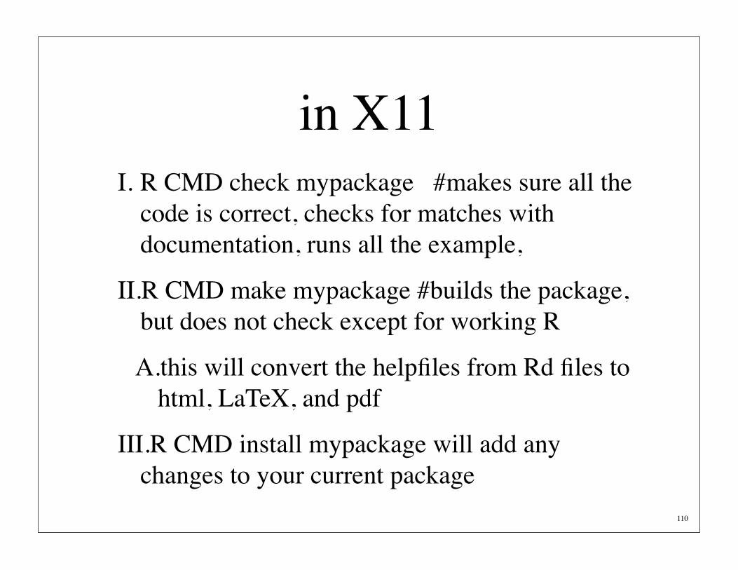
in X11I. R CMD check mypackage #makes sure all the

code is correct, checks for matches with documentation, runs all the example,

II.R CMD make mypackage #builds the package, but does not check except for working R

A.this will convert the helpfiles from Rd files to html, LaTeX, and pdf

III.R CMD install mypackage will add any changes to your current package

110

Using X11 to check packages

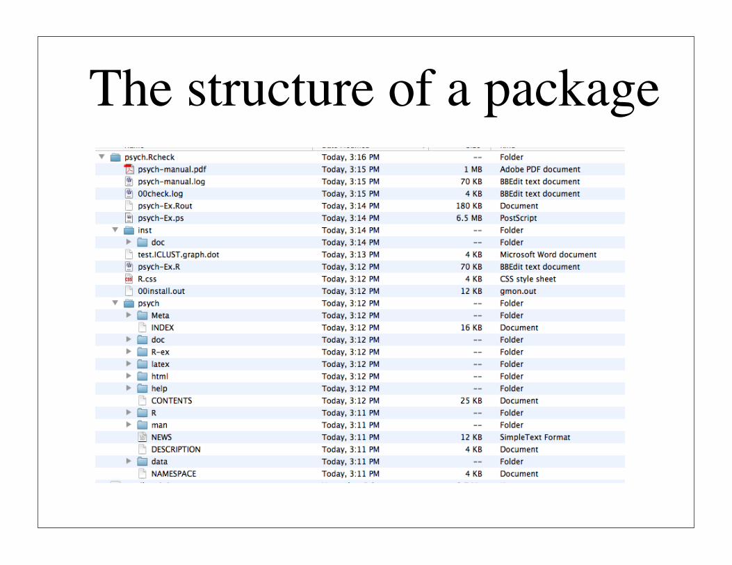
The structure of a package

The package

R CMD build psych

R in the classroomI. Undergraduate statistics and research

methods

A.describe, pairs.panels, anova, lm

B. plot, curve, etc.

C. see tutorials for 205 and 371

D.simulations of data for simulated studies

E. Examples of complex models

0 1000 2000 3000 4000 5000

-40

040

80

Action Tendencies over time

time

actio

n t

en

de

ncy

0 1000 2000 3000 4000 5000

0100

300

Actions over time

time

action

R in the classroom

I. Graduate

A.data simulations

B. data analysis

C. longer tutorial

an introduction to r: a short course part ii

Documents