an introduction to stochastic modeling · an introduction to stochastic modeling / howard m....
TRANSCRIPT

An IntroductionTo StochasticModeling
Howard M.TaylorSamuel Karlin

An Introduction toStochastic ModelingThird Edition


An Introduction toStochastic ModelingThird Edition
Howard M. TaylorStatistical ConsultantOnancock, Vi ginia
Samuel KarlinDepartment of MathematicsStanford UniversityStanford, California
OAcademic PressSan Diego London BostonNew York Sydney Tokyo Toronto

This book is printed on acid-free paper.
Copyright © 1998, 1994, 1984 by Academic Press
All rights reserved.No part of this publication may be reproduced or
transmitted in any form or by any means, electronic
or mechanical, including photocopy, recording, or
any information storage and retrieval system, without
permission in writing from the publisher.
Permissions may be sought directly from Elsevier's Science and Technology Rights Department inOxford, UK. Phone: (44) 1865 843830, Fax: (44) 1865 853333, c-mail: [email protected] may also complete your request on-line via the Elsevier homepage: httpJ/www.elseviercom byselecting 'Customer Support' and then 'Obtaining Permissions'.
ACADEMIC PRESS
An Imprint of Elsevier
525 B St., Suite 1900, San Diego, California 92101-4495, USA
1300 Boylston Street, Chestnut Hill, MA 02167, USA
http://www.apnet.com
Academic Press Limited
24-28 Oval Road, London NW 1 7DX, UK
http://www.hbuk.co.uk/ap/
Library of Congress Cataloging-in-Publication Data
Taylor, Howard M.
An introduction to stochastic modeling / Howard M. Taylor, Samuel
Karlin. - 3rd ed.p. cm.
Includes bibliographical references (p. - ) and index.
ISBN-13: 978-0-12-684887-8 ISBN-10: 0-12-684887-4
1. Stochastic processes. I. Karlin, Samuel. II. Title.QA274.T35 1998
003'.76--dc2l
ISBN-13: 978-0-12-684887-8
ISBN-10: 0-12-684887-4
PRINTED IN THE UNITED STATES OF AMERICA
05060708 IP 987654

Contents
Preface ix
I Introduction 1
1. Stochastic Modeling 1
2. Probability Review 63. The Major Discrete Distributions 244. Important Continuous Distributions 335. Some Elementary Exercises 436. Useful Functions, Integrals, and Sums 53
II Conditional Probability and ConditionalExpectation 57
1. The Discrete Case 572. The Dice Game Craps 643. Random Sums 704. Conditioning on a Continuous Random Variable 795. Martingales* 87
III Markov Chains: Introduction 95
1. Definitions 952. Transition Probability Matrices of a Markov Chain 1003. Some Markov Chain Models 1054. First Step Analysis 1165. Some Special Markov Chains 1356. Functionals of Random Walks and Success Runs 151
*Stars indicate topics of a more advanced or specialized nature.

vi Contents
7. Another Look at First Step Analysis* 1698. Branching Processes* 1779. Branching Processes and Generating Functions* 184
IV The Long Run Behavior of Markov Chains 199
1. Regular Transition Probability Matrices 1992. Examples 2153. The Classification of States 2344. The Basic Limit Theorem of Markov Chains 2455. Reducible Markov Chains* 258
V Poisson Processes 267
1. The Poisson Distribution and the Poisson Process 2672. The Law of Rare Events 2793. Distributions Associated with the Poisson Process 2904. The Uniform Distribution and Poisson Processes 2975. Spatial Poisson Processes 3116. Compound and Marked Poisson Processes 318
VI Continuous Time Markov Chains 333
1. Pure Birth Processes 3332. Pure Death Processes 3453. Birth and Death Processes 3554. The Limiting Behavior of Birth and Death
Processes 3665. Birth and Death Processes with Absorbing States 3796. Finite State Continuous Time Markov Chains 3947. A Poisson Process with a Markov Intensity* 408
VII Renewal Phenomena 419
1. Definition of a Renewal Process andRelated Concepts 419
2. Some Examples of Renewal Processes 4263. The Poisson Process Viewed as a Renewal
Process 432
*Stars indicate topics of a more advanced or specialized nature.

Contents vii
4. The Asymptotic Behavior of Renewal Processes 4375. Generalizations and Variations on Renewal
Processes 447
6. Discrete Renewal Theory* 457
VIII Brownian Motion and Related Processes 473
1. Brownian Motion and Gaussian Processes 4732. The Maximum Variable and the Reflection Principle 4913. Variations and Extensions 4984. Brownian Motion with Drift 5085. The Ornstein-Uhlenbeck Process* 524
IX Queueing Systems 541
1. Queueing Processes 5412. Poisson Arrivals, Exponential Service Times 5473. General Service Time Distributions 5584. Variations and Extensions 5675. Open Acyclic Queueing Networks 5816. General Open Networks 592
Further Reading 601
Answers to Exercises 603
Index 625
*Stars indicate topics of a more advanced or specialized nature.


Preface to the First Edition
Stochastic processes are ways of quantifying the dynamic relationships ofsequences of random events. Stochastic models play an important role inelucidating many areas of the natural and engineering sciences. They canbe used to analyze the variability inherent in biological and medicalprocesses, to deal with uncertainties affecting managerial decisions andwith the complexities of psychological and social interactions, and to pro-vide new perspectives, methodology, models, and intuition to aid in othermathematical and statistical studies.
This book is intended as a beginning text in stochastic processes for stu-dents familiar with elementary probability calculus. Its aim is to bridgethe gap between basic probability know-how and an intermediate-levelcourse in stochastic processes-for example, A First Course in StochasticProcesses, by the present authors.
The objectives of this book are three: (1) to introduce students to thestandard concepts and methods of stochastic modeling; (2) to illustrate therich diversity of applications of stochastic processes in the sciences; and(3) to provide exercises in the application of simple stochastic analysis toappropriate problems.
The chapters are organized around several prototype classes of sto-chastic processes featuring Markov chains in discrete and continuoustime, Poisson processes and renewal theory, the evolution of branchingevents, and queueing models. After the concluding Chapter IX, we pro-vide a list of books that incorporate more advanced discussions of severalof the models set forth in this text.

Preface to the Third Edition
The purposes, level, and style of this new edition conform to the tenets setforth in the original preface. We continue with our objective of introduc-ing some theory and applications of stochastic processes to students hav-ing a solid foundation in calculus and in calculus-level probability, butwho are not conversant with the "epsilon-delta" definitions of mathemat-ical analysis. We hope to entice students towards the deeper study ofmathematics that is prerequisite to further work in stochastic processes byshowing the myriad and interesting ways in which stochastic models canhelp us understand the real world.
We have removed some topics and added others. We added a small sec-tion on martingales that includes an example suggesting the martingaleconcept as appropriate for modeling the prices of assets traded in a perfectmarket. A new chapter introduces the Brownian motion process and in-cludes several applications of it and its variants in financial modeling. Inthis chapter the Black-Scholes formula for option pricing is evaluated andcompared with some reported prices of options. A Poisson process whoseintensity is itself a stochastic process is described in another new section.
Some treatments have been updated. The law of rare events is presentedvia an inequality that measures the accuracy of a Poisson approximationfor the distribution of the sum of independent, not necessarily identicallydistributed, Bernoulli random variables. We have added the shot noisemodel and related it to a random sum.
The text contains more than 250 exercises and 350 problems. Exercisesare elementary drills intended to promote active learning, to develop fa-miliarity with concepts through use. They often simply involve the sub-stitution of numbers into given formulas, or reasoning one or two stepsaway from a definition. They are the kinds of simple questions that we, as

instructors, hope that students would pose and answer for themselves asthey read a text. Answers to the exercises are given at the end of the bookso that students may gauge their understanding as they go along.
Problems are more difficult. Some involve extensive algebraic or cal-culus manipulation. Many are "word problems" wherein the student isasked, in effect, to model some described scenario. As in formulating amodel, the first step in the solution of a word problem is often a sentenceof the form "Let x = ...." A manual containing the solutions to the prob-lems is available from the publisher.
A reasonable strategy on the part of the teacher might be to hold stu-dents responsible for all of the exercises, but to require submitted solu-tions only to selected problems. Every student should attempt a represen-tative selection of the problems in order to develop his or her ability tocarry out stochastic modeling in his or her area of interest.
A small number of problems are labeled "Computer Challenges." Thesecall for more than pencil and paper for their analyses, and either simula-tion, numerical exploration, or symbol manipulation may prove helpful.Computer Challenges are meant to be open-ended, intended to explorewhat constitutes an answer in today's world of computing power. Theymight be appropriate as part of an honors requirement.
Because our focus is on stochastic modeling, in some instances we haveomitted a proof and contented ourselves with a precise statement of aresult and examples of its application. All such omitted proofs may befound in A First Course in Stochastic Processes, by the present authors.In this more advanced text, the ambitious student will also find additionalmaterial on martingales, Brownian motion, and renewal processes, andpresentations of several other classes of stochastic processes.

To the Instructor
If possible, we recommend having students skim the first two chapters, re-ferring as necessary to the probability review material, and starting thecourse with Chapter III, on Markov chains. A one quarter course adaptedto the junior-senior level could consist of a cursory (one-week) review ofChapters I and II, followed in order by Chapters III through VI. For inter-ested students, Chapters VII, VIII, and IX discuss other currently activeareas of stochastic modeling. Starred sections contain material of a moreadvanced or specialized nature.
Acknowledgments
Many people helped to bring this text into being. We gratefully acknowl-edge the help of Anna Karlin, Shelley Stevens, Karen Larsen, andLaurieann Shoemaker. Chapter IX was enriched by a series of lectures onqueueing networks given by Ralph Disney at The Johns Hopkins Univer-sity in 1982. Alan Karr, Ivan Johnstone, Luke Tierney, Bob Vanderbei,and others besides ourselves have taught from the text, and we have prof-ited from their criticisms. Finally, we are grateful for improvements sug-gested by the several generations of students who have used the book overthe past few years and have given us their reactions and suggestions.

Chapter IIntroduction
1. Stochastic Modeling
A quantitative description of a natural phenomenon is called a mathe-matical model of that phenomenon. Examples abound, from the simpleequation S = Zgt2 describing the distance S traveled in time t by a fallingobject starting at rest to a complex computer program that simulates abiological population or a large industrial system.
In the final analysis, a model is judged using a single, quite pragmatic,factor, the model's usefulness. Some models are useful as detailed quanti-tative prescriptions of behavior, as for example, an inventory model thatis used to determine the optimal number of units to stock. Another modelin a different context may provide only general qualitative informationabout the relationships among and relative importance of several factorsinfluencing an event. Such a model is useful in an equally important butquite different way. Examples of diverse types of stochastic models arespread throughout this book.
Such often mentioned attributes as realism, elegance, validity, andreproducibility are important in evaluating a model only insofar as theybear on that model's ultimate usefulness. For instance, it is both unrealis-tic and quite inelegant to view the sprawling city of Los Angeles as a geo-metrical point, a mathematical object of no size or dimension. Yet it isquite useful to do exactly that when using spherical geometry to derive aminimum-distance great circle air route from New York City, another"point."

2 I Introduction
There is no such thing as the best model for a given phenomenon. Thepragmatic criterion of usefulness often allows the existence of two ormore models for the same event, but serving distinct purposes. Considerlight. The wave form model, in which light is viewed as a continuous flow,is entirely adequate for designing eyeglass and telescope lenses. In con-trast, for understanding the impact of light on the retina of the eye, thephoton model, which views light as tiny discrete bundles of energy, ispreferred. Neither model supersedes the other; both are relevant anduseful.
The word "stochastic" derives from the Greed to aim, toguess) and means "random" or "chance." The antonym is "sure," "deter-ministic," or "certain." A deterministic model predicts a single outcomefrom a given set of circumstances. A stochastic model predicts a set ofpossible outcomes weighted by their likelihoods, or probabilities. A coinflipped into the air will surely return to earth somewhere. Whether it landsheads or tails is random. For a "fair" coin we consider these alternativesequally likely and assign to each the probability 12.
However, phenomena are not in and of themselves inherently stochas-tic or deterministic. Rather, to model a phenomenon as stochastic or de-terministic is the choice of the observer. The choice depends on the ob-server's purpose; the criterion for judging the choice is usefulness. Mostoften the proper choice is quite clear, but controversial situations do arise.If the coin once fallen is quickly covered by a book so that the outcome"heads" or "tails" remains unknown, two participants may still usefullyemploy probability concepts to evaluate what is a fair bet between them;that is, they may usefully view the coin as random, even though most peo-ple would consider the outcome now to be fixed or deterministic. As a lessmundane example of the converse situation, changes in the level of a largepopulation are often usefully modeled deterministically, in spite of thegeneral agreement among observers that many chance events contributeto their fluctuations.
Scientific modeling has three components: (i) a natural phenomenonunder study, (ii) a logical system for deducing implications about the phe-nomenon, and (iii) a connection linking the elements of the natural systemunder study to the logical system used to model it. If we think of thesethree components in terms of the great-circle air route problem, the nat-ural system is the earth with airports at Los Angeles and New York; thelogical system is the mathematical subject of spherical geometry; and the

1. Stochastic Modeling 3
two are connected by viewing the airports in the physical system as pointsin the logical system.
The modern approach to stochastic modeling is in a similar spirit. Na-ture does not dictate a unique definition of "probability," in the same waythat there is no nature-imposed definition of "point" in geometry. "Proba-bility" and "point" are terms in pure mathematics, defined only throughthe properties invested in them by their respective sets of axioms. (SeeSection 2.8 for a review of axiomatic probability theory.) There are, how-ever, three general principles that are often useful in relating or connect-ing the abstract elements of mathematical probability theory to a real ornatural phenomenon that is to be modeled. These are (i) the principle ofequally likely outcomes, (ii) the principle of long run relative frequency,and (iii) the principle of odds making or subjective probabilities. Histori-cally, these three concepts arose out of largely unsuccessful attempts todefine probability in terms of physical experiences. Today, they are rele-vant as guidelines for the assignment of probability values in a model, andfor the interpretation of the conclusions of a model in terms of the phe-nomenon under study.
We illustrate the distinctions between these principles with a long ex-periment. We will pretend that we are part of a group of people who de-cide to toss a coin and observe the event that the coin will fall heads up.This event is denoted by H, and the event of tails, by T.
Initially, everyone in the group agrees that Pr{H} = ;. When asked why,people give two reasons: Upon checking the coin construction, they be-lieve that the two possible outcomes, heads and tails, are equally likely;and extrapolating from past experience, they also believe that if the coinis tossed many times, the fraction of times that heads is observed will beclose to one-half.
The equally likely interpretation of probability surfaced in the works ofLaplace in 1812, where the attempt was made to define the probability ofan event A as the ratio of the total number of ways that A could occur tothe total number of possible outcomes of the experiment. The equallylikely approach is often used today to assign probabilities that reflect somenotion of a total lack of knowledge about the outcome of a chance phe-nomenon. The principle requires judicious application if it is to be useful,however. In our coin tossing experiment, for instance, merely introducingthe possibility that the coin could land on its edge (E) instantly results inPr(H) = Pr{T} = Pr{E} = ;.
4 I Introduction
The next principle, the long run relative frequency interpretation ofprobability, is a basic building block in modern stochastic modeling, madeprecise and justified within the axiomatic structure by the law of largenumbers. This law asserts that the relative fraction of times in which anevent occurs in a sequence of independent similar experiments ap-proaches, in the limit, the probability of the occurrence of the event on anysingle trial.
The principle is not relevant in all situations, however. When the sur-geon tells a patient that he has an 80-20 chance of survival, the surgeonmeans, most likely, that 80 percent of similar patients facing similarsurgery will survive it. The patient at hand is not concerned with the longrun, but in vivid contrast, is vitally concerned only in the outcome of his,the next, trial.
Returning to the group experiment, we will suppose next that the coin isflipped into the air and, upon landing, is quickly covered so that no one cansee the outcome. What is Pr{H} now? Several in the group argue that theoutcome of the coin is no longer random, that Pr{H} is either 0 or 1, andthat although we don't know which it is, probability theory does not apply.
Others articulate a different view, that the distinction between "ran-dom" and "lack of knowledge" is fuzzy, at best, and that a person with asufficiently large computer and sufficient information about such factorsas the energy, velocity, and direction used in tossing the coin could havepredicted the outcome, heads or tails, with certainty before the toss.Therefore, even before the coin was flipped, the problem was a lack ofknowledge and not some inherent randomness in the experiment.
In a related approach, several people in the group are willing to bet witheach other, at even odds, on the outcome of the toss. That is, they are will-ing to use the calculus of probability to determine what is a fair bet, with-out considering whether the event under study is random or not. The use-fulness criterion for judging a model has appeared.
While the rest of the mob were debating "random" versus "lack ofknowledge," one member, Karen, looked at the coin. Her probability forheads is now different from that of everyone else. Keeping the coin cov-ered, she announces the outcome "Tails," whereupon everyone mentallyassigns the value Pr{H} = 0. But then her companion, Mary, speaks upand says that Karen has a history of prevarication.
The last scenario explains why there are horse races; different peopleassign different probabilities to the same event. For this reason, probabil-

1. Stochastic Modeling 5
ities used in odds making are often called subjective probabilities. Then,odds making forms the third principle for assigning probability values inmodels and for interpreting them in the real world.
The modern approach to stochastic modeling is to divorce the definitionof probability from any particular type of application. Probability theoryis an axiomatic structure (see Section 2.8), a part of pure mathematics. Itsuse in modeling stochastic phenomena is part of the broader realm of sci-ence and parallels the use of other branches of mathematics in modelingdeterministic phenomena.
To be useful, a stochastic model must reflect all those aspects of thephenomenon under study that are relevant to the question at hand. In ad-dition, the model must be amenable to calculation and must allow the de-duction of important predictions or implications about the phenomenon.
1.1. Stochastic Processes
A stochastic process is a family of random variables X where t is a para-meter running over a suitable index set T. (Where convenient, we willwrite X(t) instead of X,.) In a common situation, the index t correspondsto discrete units of time, and the index set is T = {0, 1, 2, . . .}. In thiscase, X, might represent the outcomes at successive tosses of a coin, re-peated responses of a subject in a learning experiment, or successive ob-servations of some characteristics of a certain population. Stochasticprocesses for which T = [0, c) are particularly important in applications.Here t often represents time, but different situations also frequently arise.For example, t may represent distance from an arbitrary origin, and X, maycount the number of defects in the interval (0, t] along a thread, or thenumber of cars in the interval (0, t] along a highway.
Stochastic processes are distinguished by their state space, or the rangeof possible values for the random variables X by their index set T, and bythe dependence relations among the random variables X,. The most widelyused classes of stochastic processes are systematically and thoroughlypresented for study in the following chapters, along with the mathemati-cal techniques for calculation and analysis that are most useful with theseprocesses. The use of these processes as models is taught by example.Sample applications from many and diverse areas of interest are an inte-gral part of the exposition.

6 I Introduction
2. Probability Review*
This section summarizes the necessary background material and estab-lishes the book's terminology and notation. It also illustrates the level ofthe exposition in the following chapters. Readers who find the major partof this section's material to be familiar and easily understood should haveno difficulty with what follows. Others might wish to review their proba-bility background before continuing.
In this section statements frequently are made without proof. Thereader desiring justification should consult any elementary probabilitytext as the need arises.
2.1. Events and Probabilities
The reader is assumed to be familiar with the intuitive concept of an event.(Events are defined rigorously in Section 2.8, which reviews the axiomaticstructure of probability theory.)
Let A and B be events. The event that at least one of A or B occurs iscalled the union of A and B and is written A U B; the event that both occuris called the intersection of A and B and is written A fl B, or simply AB.This notation extends to finite and countable sequences of events. Givenevents A A2, ... , the event that at least one occurs is written A, U A, U
= U i A;, the event that all occur is written A, fl A, fl = f1;=, A;.The probability of an event A is written Pr{A }. The certain event, de-
noted by (1, always occurs, and Pr{ Cl } = 1. The impossible event, de-noted by 0, never occurs, and Pr{O} = 0. It is always the case that 0 sPr(A) : 1 for any event A.
Events A, B are said to be disjoint if A fl B = 0; that is, if A and Bcannot both occur. For disjoint events A, B we have the addition lawPr{A U B) = Pr(A) + Pr{B}. A stronger form of the addition law is asfollows: Let A,, A,, . . . be events with A; and A; disjoint whenever i 0 j.Then Pr(U , A; ) = Ex , Pr{A;}. The addition law leads directly to the law
* Many readers will prefer to omit this review and move directly to Chapter III, onMarkov chains. They can then refer to the background material that is summarized in theremainder of this chapter and in Chapter II only as needed.

2. Probability Review 7
of total probability: Let A,, A,, . . . be disjoint events for which fl = A, U A,U .... Equivalently, exactly one of the events A A,. . . will occur. The lawof total probability asserts that Pr{B} = 7-;_, Pr(B fl A;} for any event B.The law enables the calculation of the probability of an event B fromthe sometimes more easily determined probabilities Pr{B fl A;}, where i= 1, 2, .... Judicious choice of the events A; is prerequisite to the prof-itable application of the law.
Events A and B are said to be independent if Pr{A fl B) = Pr{A} XPr{B}. Events A,, A,, ... are independent if
Pr{A;1 fl A;, fl ... fl A; } = Pr(A;d Pr{A;,} ... Pr{A; }
for every finite set of distinct indices i i,, . . . , i,,.
2.2 Random Variables
An old-fashioned but very useful and highly intuitive definition describesa random variable as a variable that takes on its values by chance. In Sec-tion 2.8, we sketch the modern axiomatic structure for probability theoryand random variables. The older definition just given serves quite ade-quately, however, in virtually all instances of stochastic modeling. Indeed,this older definition was the only approach available for well over a cen-tury of meaningful progress in probability theory and stochasticprocesses.
Most of the time we adhere to the convention of using capital letterssuch as X, Y, Z to denote random variables, and lowercase letters such asx, y, z for real numbers. The expression (X:5 x) is the event that the ran-dom variable X assumes a value that is less than or equal to the real num-ber x. This event may or may not occur, depending on the outcome of theexperiment or phenomenon that determines the value for the random vari-able X. The probability that the event occurs is written Pr{X <- x). Allow-ing x to vary, this probability defines a function
F(x) = Pr{X x}, -oo < x < +o,
called the distribution function of the random variable X. Where severalrandom variables appear in the same context, we may choose to distin-guish their distribution functions with subscripts, writing, for example,FX(6) = Pr(X --- ) and F,.(6) = Pr{ Y 6}, defining the distribution

8 I Introduction
functions of the random variables X and Y, respectively, as functions ofthe real variable 6.
The distribution function contains all the information available about arandom variable before its value is determined by experiment. We have,for instance, Pr{X > a} = 1 - F(a), Pr{a < X <_ b} = F(b) - F(a), andPr{X = x} = F(x) - lim.10 F(x - e) = F(x) - F(x -).
A random variable X is called discrete if there is a finite or denumerableset of distinct values x,, x2, ... such that a, = Pr{X = x; } > 0 for i = 1, 2,... and Y a; = 1. The function
p(x,) = px(x;) = a; for i = 1, 2, ... (2.1)
is called the probability mass function for the random variable X and is re-lated to the distribution function via
p(x;) = F(x,) - F(x; -) and F(x) p(x;).xi x
The distribution function for a discrete random variable is a step function,which increases only in jumps, the size of the jump at x; being p(x;).
If Pr{X = x} = 0 for every value of x, then the random variable Xis called continuous and its distribution function F(x) is a continuousfunction of x. If there is a nonnegative function f(x) = fx(x) defined for-- < x < - such that
n
Pr{a<X<_b} = Jf(x)dx for -oo<a<b< co, (2.2)a
then f(x) is called the probability density function for the random variableX. If X has a probability density function f(x), then X is continuous and
F(x) f(6) de, -o-<x<-.
If F(x) is differentiable in x, then X has a probability density functiongiven by
f(x) = d F(x) = F'(x), -00 < x < 00.. (2.3)
In differential form, (2.3) leads to the informal statement
Pr { x < X < x + dx } = F(x + dx) - F(x) = dF(x) = f (x) dx. (2.4)

2. Probability Review 9
We consider (2.4) to be a shorthand version of the more precise statement
Pr{x<X<-x+Ax} =f(x)L x+o(Ox), Ax 10, (2.5)
where o(Ax) is a generic remainder term of order less than Ox as Ax 10.That is, o(1x) represents any term for which lima,10 o(Ax)/Ax = 0. By thefundamental theorem of calculus, equation (2.5) is valid whenever theprobability density function is continuous at x.
While examples are known of continuous random variables that do notpossess probability density functions, they do not arise in stochastic modelsof common natural phenomena.
2.3. Moments and Expected Values
If X is a discrete random variable, then its mth moment is given by
E[X",] x' Pr(X = x;}, (2.6)
[where the x; are specified in (2.1)] provided that the infinite sum con-verges absolutely. Where the infinite sum diverges, the moment is said notto exist. If X is a continuous random variable with probability densityfunctionf(x), then its mth moment is given by
E[X"]= J x";f(x) dx, (2.7)
provided that this integral converges absolutely.The first moment, corresponding to m = 1, is commonly called the
mean or expected value of X and written m, or µX. The mth central mo-ment of X is defined as the mth moment of the random variable X - tt,provided that p exists. The first central moment is zero. The second cen-tral moment is called the variance of X and written oX or Var[X]. We havethe equivalent formulas Var[X] = E[(X - µ)2] = E[X2] - Al.
The median of a random variable X is any value v with the property that
Pr{X ? v) ? and Pr{X :s v} ? Z.
If X is a random variable and g is a function, then Y = g(X) is also a

10 I Introduction
random variable. If X is a discrete random variable with possible valuesx x2, .... then the expectation of g(X) is given by
E[g(X)] _ Y, g(x;) Pr{X = x;}, (2.8)
provided that the sum converges absolutely. If X is continuous and has theprobability density function fx, then the expected value of g(X) is evalu-ated from
E[g(X)] = J g(x)fx(x) dx. (2.9)
The general formula, covering both the discrete and continuous cases, is
E[g(X)] = f g(x) dFx(x), (2.10)
where Fx is the distribution function of the random variable X. Technicallyspeaking, the integral in (2.10) is a Lebesgue-Stieltjes integral. We do notrequire knowledge of such integrals in this text, but interpret (2.10) to sig-nify (2.8) when X is a discrete random variable, and to represent (2.9)when X possesses a probability density fx.
Let F,(y) = Pr{ Y <_ y} denote the distribution function for Y = g(X).When X is a discrete random variable, then
E[Y] _ y; Pr{Y = y;}
_ g(x;) Pr{X = x;}
if y; = g(x;) and provided that the second sum converges absolutely. Ingeneral,
E[Y] = JydF)(y)
J g(x) dFx(x)(2.11)
If X is a discrete random variable, then so is Y = g(X). It may be, how-ever, that X is a continuous random variable while Y is discrete (the readershould provide an example). Even so, one may compute E[Y] from eitherform in (2.11) with the same result.

2. Probability Review 11
2.4. Joint Distribution Functions
Given a pair (X, Y) of random variables, their joint distribution functionis the function Fxr of two real variables given by
Fx,.(x, y) = F(x, y) = Pr(X <- x and Y:5 y).
Usually, the subscripts X, Y will be omitted, unless ambiguity is possible.A joint distribution function Fxr is said to possess a (joint) probability den-sity if there exists a functionfxr of two real variables for which
x 'vFxr(x, y) = f f -l) di? d6 for all x, y.
The function Fx(x) = lim,.,x F(x, y) is a distribution function, called themarginal distribution function of X. Similarly, F,.(y) = lim, F(x, y) isthe marginal distribution function of Y. If the distribution function F pos-sesses the joint density function f, then the marginal density functions forX and Y are given, respectively, by
+x +x
fx(x) = J f(x, y) dy and f(y) f f(x, y) dx.
If X and Y are jointly distributed, then E[X + Y] = E[X] + E[Y], pro-vided only that all these moments exist.
Independence
If it happens that F(x, y) = FF(x) X F,.(y) for every choice of x, y, then therandom variables X and Y are said to be independent. If X and Y are inde-pendent and possess a joint density function f(x, y), then necessarilyf(x, y) = fx(x)f,.(y) for all x, y.
Given jointly distributed random variables X and Y having means µxand µ, and finite variances, the covariance of X and Y, written o orCov[X, Y], is the product moment o-xr = E[(X - µx)(Y - Ixy)] =E[XY] - µxµy, and X and Y are said to be uncorrelated if their covarianceis zero, that is, o-xy = 0. Independent random variables having finite vari-ances are uncorrelated, but the converse is not true; there are uncorrelatedrandom variables that are not independent.

12 I Introduction
Dividing the covariance o-, by the standard deviations ox and o-, de-fines the correlation coefficient p = o-x,I oxo'r for which -1 p < + 1.
The joint distribution function of any finite collection X ... , X,, of ran-dom variables is defined as the function
F(x,, ... , x,,) = Fx,.....x,,(x1, . . . , x,.)
= Pr(X1 :5 x1,...,X.:x
If F(x,,... , x,,) = Fx,(x,) Fx (x,,) for all values of x,, ... , x,,, then therandom variables X . . . , X,, are said to be independent.
A joint distribution function F(x...... x,,) is said to have a probabilitydensity function f(6,..... if
x, x
F(x,,...,x,) = J ... J .f( .,...,-x x
for all values of x,, . . . , x,,.
Expectation
For jointly distributed random variables X ... , X,, and arbitrary func-tions h,, . . . , h,, of n variables each,
In Ill
E1 h;(X,, ... , 7, E[h;(X......l= l=I
provided only that all these moments exist.
2.5. Sums and Convolutions
If X and Y are independent random variables having distribution functionsFx and F, respectively, then the distribution function of their sum Z = X+ Y is the convolution of Fx and F,.:
+x +x
Fz(z) = J Fx(z - ) J Fr(z - 71) dFx(71). (2.12)-x -x
If we specialize to the situation where X and Y have the probability densi-

2. Probability Review 13
tiesfx and f,., respectively, then the density function fz of the sum Z = X +Y is the convolution of the densities fx and f,.:
x +x
fz(z) = J fx(z - 17)fr(71) dq = f ff(z - 6)fx(6) d6. (2.13)
Where X and Y are nonnegative random variables, the range of integrationis correspondingly reduced to
z Z
fz(z) = f fx(z - 71)fr(71) d'rl = Jfr(z - d for z ? 0. (2.14)0 0
If X and Y a r e independent and have respective variances o- and o ,then the variance of the sum Z = X + Y is the sum of the variances: o =o + 0-2. More generally, if X ... , X,, are independent random variableshaving variances o , ... , c,2, respectively, then the variance of the sumZ=X, +... +X is QZ= 0-; +... +o,2.
2.6. Change of Variable
Suppose that X is a random variable with probability density function fxand that g is a strictly increasing differentiable function. Then Y = g(X)defines a random variable, and the event ( Y -- y) is the same as the event{X : g-'(y)}, where g-' is the inverse function to g; i.e., y = g(x) if andonly if x = g-'(y). Thus we obtain the correspondence F,.(y) = Pr{Y : y)= Pr{X s g-'(y)} = Fx(g-'(y)) between the distribution function of Yandthat of X. Recall the differential calculus formula
dg-'=
1
=1
'
where y = g(x),dy g(x) dgldx
and use this in the chain rule of differentiation to obtain
dFy(y) - dFx(g-'(y)) = f 1where y = g(x)..= dy dy x(x)
OX),The formula
.fr(y) =1
g,(x)fx(x), where y = g(x). (2.15)
expresses the density function for Y in terms of the density for X when gis strictly increasing and differentiable.
14 I Introduction
2.7. Conditional Probability
For any events A and B, the conditional probability of A given B is writ-ten Pr{AIB} and defined by
Pr{AIB} =Pr{A fl B)
if Pr{B} > 0, (2.16)Pr{B}
and is left undefined if Pr(B) = 0. [When Pr{B} = 0, the right side of(2.16) is the indeterminate quantity o.]
In stochastic modeling, conditional probabilities are rarely procured via(2.16) but instead are dictated as primary data by the circumstances of theapplication, and then (2.16) is applied in its equivalent multiplicative form
Pr{A fl B) = Pr{AIB} Pr{B} (2.17)
to compute other probabilities. (An example follows shortly.) Central inthis role is the law of total probability, which results from substitutingPr{A fl B.) = Pr{AIB;} Pr{ B;} into Pr{A} = E;=, Pr{A fl B;}, where fl =B, U B, U and B; fl B; = 0 if i 0 j (cf. Section 2.1), to yield
xPr{A} = 7, Pr{AIB;} Pr {B;}. (2.18)
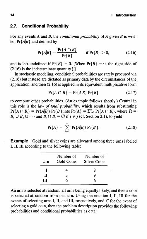
Example Gold and silver coins are allocated among three urns labeledI, II, III according to the following table:
Number of Number ofUrn Gold Coins Silver Coins
I 4 8
II 3 9III 6 6
An urn is selected at random, all urns being equally likely, and then a coinis selected at random from that urn. Using the notation I, II, III for theevents of selecting urns I, II, and III, respectively, and G for the event ofselecting a gold coin, then the problem description provides the followingprobabilities and conditional probabilities as data:

2. Probability Review 15
Pr{I} = , Pr(Gli) = ,
Pr(II) = , Pr{ GIII } = ,,_,
Pr{III} = , Pr{G1III} = 162,
and we calculate the probability of selecting a gold coin according to(2.18), viz.
Pr{G} = Pr{GII} Pr//{I} + /Pr{GIII} Pr{II} + Pr{GjIII} Pr{III}I_/'3)
+I?l3\\1 + l}) 36
As seen here, more often than not conditional probabilities are given asdata and are not the end result of calculation.
Discussion of conditional distributions and conditional expectationmerits an entire chapter (Chapter II).
2.8. Review of Axiomatic Probability Theory*
For the most part, this book studies random variables only through theirdistributions. In this spirit, we defined a random variable as a variable thattakes on its values by chance. For some purposes, however, a little moreprecision and structure are needed.
Recall that the basic elements of probability theory are
1. the sample space, a set fl whose elements w correspond to the pos-sible outcomes of an experiment;
2. the family of events, a collection of subsets A of fl: we say thatthe event A occurs if the outcome w of the experiment is an elementof A; and
3. the probability measure, a function P defined on c!; and satisfying
(a) 0 = P[Q ] <_ P[A] P[fl] = 1 for A E
(0 = the empty set)
* The material included in this review of axiomatic probability theory is not used in theremainder of the book. It is included in this review chapter only for the sake of complete-ness.

16 I Introduction
and
(b) P[u A,,] = 7 (2.19)r,=1 n=1
if the events A,, A2, ... are disjoint; i.e., if A. fl A; = 0 when i 0 j.
The triple (Il, , P) is called a probability space.
Example When there are only a denumerable number of possible out-comes, say ft = {w,, w,, ...}, we may take 9i to be the collection of allsubsets of fl. If p,, p2, ... are nonnegative numbers with Y-,, p,, = 1, theassignment
P[A] = Z, p,w,EA
determines a probability measure defined on.It is not always desirable, consistent, or feasible to take the family of
events as the collection of all subsets of (Z. Indeed, when fl is nondenu-merably infinite, it may not be possible to define a probability measure onthe collection of all subsets maintaining the properties of (2.19). In what-ever way we prescribe such that (2.19) holds, the family of eventsshould satisfy
(a) 0 is in and f is in ;
(b) A` is in whenever A is in 9, where A` w E fl; w (4 A) (2.20)is the complement of A; and
(c) A,, is in whenever A,, is in for n = 1, 2, ... .A collection of subsets of a set fl satisfying (2.20) is called a o-alge-bra. If is a o --algebra, then
i n1
C_(J A,-,
in whenever A,, is in for n = 1, 2, .... Manifestly, as a conse-quence we find that finite unions and finite intersections of members of ?are maintained in .
In this framework, a real random variable X is a real-valued functiondefined on fl fulfilling certain "measurability" conditions given here. Thedistribution function of the random variable X is formally given by

2. Probability Review 17
Pr{a<X<_b} =P[{co;a<X(c)):!5 b}]. (2.21)
In words, the probability that the random variable X takes a value in (a, b]is calculated as the probability of the set of outcomes w for which a <X(w) : b. If relation (2.21) is to have meaning, X cannot be an arbitraryfunction on fl, but must satisfy the condition that
{ w; a < X(w) : b) is in for all real a < b,
since embodies the only sets A for which P[A] is defined. In fact, by ex-ploiting the properties (2.20) of the o-algebra , we find that it is enoughto require
{ w; X(w) <_ x} is in g for all real x.
Let s4 be any o--algebra of subsets of f1. We say that X is measurable withrespect to .si, or more briefly .A-measurable, if
{ w; X(w) < x} is in . for all real x.
Thus, every real random variable is by definition 9;-measurable. Theremay, in general, be smaller o-algebras with respect to which X is alsomeasurable.
The a -algebra generated by a random variable X is defined to be thesmallest o--algebra with respect to which X is measurable. It is denoted byi(X) and consists exactly of those sets A that are in every o--algebra A forwhich X is A-measurable. For example, if X has only denumerably manypossible values x,, x2, . . . , the sets
A;= {w;X(w)=x;}, i= 1,2,...,form a countable partition of f1, i.e.,
f1 = U A;,
andi=I
A;fA;=0 ifi*j,and then P(X) includes precisely 0, f1, and every set that is the union ofsome of the A;'s.
Example For the reader completely unfamiliar with this framework,the following simple example will help illustrate the concepts. The exper-

18 I Introduction
iment consists in tossing a nickel and a dime and observing "heads" or"tails." We take SZ to be
fl = { (H, H), (H, T), (T, H), (T, T)),
where, for example, (H, T) stands for the outcome "nickel = heads, anddime = tails." We will take the collection of all subsets of fl as the fam-ily of events. Assuming each outcome in ft to be equally likely, we arriveat the probability measure:
AEI P[A] AE?0
{(H, H)}{(H, T)){ (T, H)){(T, T)}{ (H, H), (H, T) }{ (H, H), (T, H)){ (H, H), (T, T))
n{ (H, T), (T, H), (T, T))((H, H), (T, H), (T, T)){ (H, H), (H, T), (T, T))((H, H), (H, T), (T, H)){ (T, H), (T, T)){(H, T), (T, T)}{ (H, T), (T, H))
The event "nickel is heads" is ((H, H), (H, T)) and has, according to thetable, probability , as it should.Z
Let X,, be 1 if the nickel is heads, and 0 otherwise; let X, be the corre-sponding random variable for the dime; and let Z = X,, + Xd be the totalnumber of heads. As functions on fl, we have
CO E'l X"(w) X1(w) Z(w)
(H, H) 1 1 2
(H, T) 1 0 1
(T, H) 0 1 1
(T, T) 0 0 0
Finally, the a=algebras generated by X,, and Z are
0, Il, {(H, H), (H, T)), {(T, H), (T, T)},
and
9,(Z) _ 0, fl, ((H, H)), {(H, T), (T, H)), {(T, T)},
{(H, T), (T, H), (T, T)), {(H, H), (T, T)},
((H, H), (H, T), (T, H) }.

Exercises 19
contains four sets and &(Z) contains eight. Is X,, measurable withrespect to 9;(Z), or vice versa?
Every pair X, Y of random variables determines a o--algebra called theo --algebra generated by X, Y. It is the smallest a-algebra with respect towhich both X and Y are measurable. This or-algebra comprises exactlythose sets A that are in every or algebra si for which X and Y are both .-measurable. If both X and Y assume only denumerably many possible val-ues, say x,, x,, . . . and y,, y,, ... , respectively, then the sets
A;; = {w; X(co) = xi, Y(w) = y;}, i, j = 1, 2, ... ,
present a countable partition of 11, and (X, Y) consists precisely of 0,fl, and every set that is the union of some of the A,1's. Observe that X ismeasurable with respect to 5;(X, Y), and thus (X) C &(X, Y).
More generally, let {X(t ); t E T J be any family of random variables.Then the o --algebra generated by (X(t); t E T) is the smallestwith respect to which every random variable X(t), t E T, is measurable. Itis denoted by {X(t); t E T).
A special role is played by a distinguished o--algebra of sets of realnumbers. The o --algebra of Borel sets is the o--algebra generated by theidentity function f(x) = x, for x E (-cc, cc). Alternatively, the o --algebraof Borel sets is the smallest o--algebra containing every interval of theform (a, b], -x < a :5 b < +cc. A real-valued function of a real variableis said to be Borel measurable if it is measurable with respect to the o,--al-gebra of Borel sets.
Exercises
2.1. Let A and B be arbitrary, not necessarily disjoint, events. Use thelaw of total probability to verify the formula
Pr{A} = Pr{AB} + Pr{AB`},
where B` is the complementary event to B. (That is, B` occurs if and onlyif B does not occur.)
2.2. Let A and B be arbitrary, not necessarily disjoint, events. Establishthe general addition law
Pr(A U B} = Pr{A} + Pr{B} - Pr{AB}.
20 I Introduction
Hint: Apply the result of Exercise 2.1 to evaluate Pr{AB'} =Pr(A) - Pr{AB}. Then apply the addition law to the disjoint events ABand AB`*, noting that A = (AB) U (AB`).
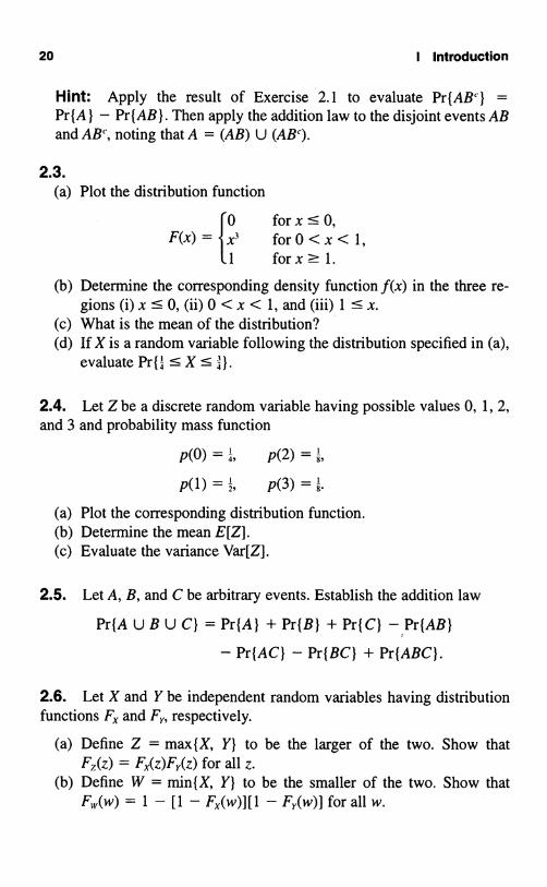
2.3.(a) Plot the distribution function
10 for x s 0,F(x) = x; for 0 < x < 1,
1 forx? 1.(b) Determine the corresponding density function f(x) in the three re-
gions (i) x : 0, (ii) 0 < x < 1, and (iii) 1 < x.(c) What is the mean of the distribution?(d) If X is a random variable following the distribution specified in (a),
evaluate Pr{; X <_}.
2.4. Let Z be a discrete random variable having possible values 0, 1, 2,and 3 and probability mass function
P(0) = ;, p(2) =
P(l) = Z, p(3) = x.
(a) Plot the corresponding distribution function.(b) Determine the mean E[Z].(c) Evaluate the variance Var[Z].
2.5. Let A, B, and C be arbitrary events. Establish the addition law
Pr{A U B U C} = Pr{A} + Pr{B} + Pr{C} - Pr{AB}
- Pr{AC} - Pr{BC} + Pr{ABC}.
2.6. Let X and Y be independent random variables having distributionfunctions F, and F, respectively.
(a) Define Z = max{X, Y} to be the larger of the two. Show thatF,(z) = FX(z)FY(z) for all z.
(b) Define W = min{X, Y} to be the smaller of the two. Show thatF,,,(w) = 1 - [I - FX(w)] [ 1 - F,.(w)] for all w.

Problems 21
2.7. Suppose X is a random variable having the probability densityfunction
f (X) - 10 elsewhere,
where R > 0 is a fixed parameter.
(a) Determine the distribution function FX(x).(b) Determine the mean E[X].(c) Determine the variance Var[X].
2.8. A random variable V has the distribution function
10 forv < 0,F(v)= 1-(1-v)A for 0<vs1,
1 forv > 1,
where A > 0 is a parameter. Determine the density function, mean, andvariance.
2.9. Determine the distribution function, mean, and variance corre-sponding to the triangular density.
X for 0 <- x 1,
,f(x)= 2-x forl10 elsewhere.
2.10. Let 1(A) be the indicator random variable associated with anevent A, defined to be one if A occurs, and zero otherwise. Define A`, thecomplement of event A, to be the event that occurs when A does not occur.Show
(a) 1{A`} = 1 - 1{A}.(b) 1{A fl B) = 1(A)1{B} = min{1{A}, 1{B}}.(c) 1{A U B) = max(1{A}, 11B}).
Problems
2.1. Thirteen cards numbered 1, ... , 13 are shuffled and dealt one at atime. Say a match occurs on deal k if the kth card revealed is card number

22 I Introduction
k. Let N be the total number of matches that occur in the thirteen cards.Determine E[N].
Hint: Write N = 1 (A,) + + 1 where Ak is the event that amatch occurs on deal k.
2.2. Let N cards carry the distinct numbers x ... , x,,. If two cards aredrawn at random without replacement, show that the correlation coeffi-cient p between the numbers appearing on the two cards is - lI(N - 1).
2.3. A population having N distinct elements is sampled with replace-ment. Because of repetitions, a random sample of size r may containfewer than r distinct elements. Let S, be the sample size necessary to getr distinct elements. Show that
E[S,]=N(1 + 1 +...+ 1 ).N N-1 N - r+l2.4. A fair coin is tossed until the first time that the same side appearstwice in succession. Let N be the number of tosses required.
(a) Determine the probability mass function for N.(b) Let A be the event that N is even and B be the event that N : 6.
Evaluate Pr{A}, Pr{B}, and Pr{AB}.
2.5. Two players, A and B, take turns on a gambling machine until oneof them scores a success, the first to do so being the winner. Their proba-bilities for success on a single play are p for A and q for B, and successiveplays are independent.
(a) Determine the probability that A wins the contest given that A playsfirst.
(b) Determine the mean number of plays required, given that A wins.
2.6. A pair of dice is tossed. If the two outcomes are equal, the dice aretossed again, and the process repeated. If the dice are unequal, their sumis recorded. Determine the probability mass function for the sum.
2.7. Let U and W be jointly distributed random variables. Show that Uand W are independent if
Pr{U>uand W>w} =Pr{U>u} Pr{W>w} forallu,w.

Problems 23
2.8. Suppose X is a random variable with finite mean µ and variance 0-',and Y = a + bX for certain constants a, b ± 0. Determine the mean andvariance for Y.
2.9. Determine the mean and variance for the probability mass function
2(n - k)p(k) = n(n - 1 )
for k = 1, 2, ... , n.
2.10. Random variables X and Y are independent and have the proba-bility mass functions
Px(0) = Pv(l) = b,
Px(3) = >, Pr(2) = 3,
Ps-(3) = ;.
Determine the probability mass function of the sum Z = X + Y.
2.11. Random variables U and V are independent and have the proba-bility mass functions
Pu(0) = ,, P,(l) = i,
Pu(l) = , p,(2) = .
pu(2) = ,Determine the probability mass function of the sum W = U + V.
2.12. Let U, V, and W be independent random variables with equal vari-ances o.'-. Define X = U + W and Y = V - W. Find the covariance be-tween X and Y.
2.13. Let X and Y be independent random variables each with the uni-form probability density function
_ 1 for0<x<l,f(x) -
I0elsewhere.
Find the joint probability density function of U and V, where U =max{X, Y} and V = min{X, Y}.

24 I Introduction
3. The Major Discrete Distributions
The most important discrete probability distributions and their relevantproperties are summarized in this section. The exposition is brief, sincemost readers will be familiar with this material from an earlier course inprobability.
3.1. Bernoulli Distribution
A random variable X following the Bernoulli distribution with parameterp has only two possible values, 0 and 1, and the probability mass functionis p(l) = p and p(O) = 1 - p, where 0 < p < 1. The mean and varianceare E[X] = p and Var[X] = p(1 - p), respectively.
Bernoulli random variables occur frequently as indicators of events.The indicator of an event A is the random variable
1(A) = 1A = {0if A occurs,if A does not occur.
(3.1)
Then 1A is a Bernoulli random variable with parameter p = E[lA] _Pr{A}.
The simple expedient of using indicators often reduces formidable cal-culations into trivial ones. For example, let a a2, ... , a,, be arbitrary realnumbers and A, , A2, ... , A,, be events, and consider the problem of show-ing that
n it
17 a;aj Pr(A; fl Aj) ? 0. (3.2)i=tj=t
Attacked directly, the problem is difficult. But bringing in the indicators1(A) and observing that
0 ail(A)} a.1(A)}{ ajl(A)}
It n lI n
_ Y Y a aj1(A;)1(A) = Y 7, a;aj1(A, fl Aj)1=1j=I i=1j=1

3. The Major Discrete Distributions 25
gives, after taking expectations,
n it
0 E{{>a,1(A)} ] = 17 ara;E[uA, n A;)]
-, i=i;=I
_ a;a; Pr{A; f1 A;},t=I j=I
and the demonstration of (3.2) is complete.
3.2. Binomial Distribution
Consider independent events A A2, .... A,,, all having the same proba-bility p = Pr{A;} of occurrence. Let Y count the total number of eventsamong A ... , A that occur. Then Y has a binomial distribution with pa-rameters n and p. The probability mass function is
py(k) = Pr{Y = k}
n!= k!(n - k)! Pk(1 - P)11-k for k = 0,1,..., n.
(3.3)
Writing Y as a sum of indicators in the form Y = 1(A,) + +makes it easy to determine the moments
E[Y] = E[1(A,)] + + np,
and using independence, we can also determine that
Var[Y] = Var[1(A,)] + + np(1 - p).
Briefly, we think of a binomial random variable as counting the numberof "successes" in n independent trials where there is a constant probabil-ity p of success on any single trial.
3.3. Geometric and Negative Binomial Distributions
Let A A,, . .. be independent events having a common probability p =Pr{A;} of occurrence. Say that trial k is a success (S) or failure (F)

26 I Introduction
according as A, occurs or not, and let Z count the number of failures priorto the first success. To be precise, Z = k if and only if 1(A,) = 0, . . . ,1(Ak)= 0, and 1(Ak+0 = 1. Then Z has a geometric distribution with parameterp. The probability mass function is
pz(k) = p(1 - p)k for k = 0, 1, ... , (3.4)
and the first two moments are
E[Z] = 1 P ; Var[Z] = 1 , PP P"
Sometimes the term "geometric distribution" is used in referring to theprobability mass function
Pz,(k) = p(1 - p)k_I for k = 1, 2..... (3.5)
This is merely the distribution of the random variable Z' = 1 + Z, thenumber of trials until the first success. Hence E[Z'] = 1 + E[Z] = 11p,and Var[Z'] = Var[Z] = (1 - p)lp2.
Now fix an integer r ? I and let W, count the number of failures ob-served before the rth success in A, A,, .... Then W has a negative bi-nominal distribution with parameters r and p. The event W,. = k calls for(A) exactly r - 1 successes in the first k + r - 1 trials, followed by, (B)a success on trial k + r. The probability for (A) is obtained from a bino-mial distribution, and the probability for (B) is simply p, which leads tothe following probability mass function for W,.:
p(k) = Pr{ W, = k) _(r - - 1)!
p,(l - p)k, k = 0, 1, .... (3.6)
Another way of writing W, is as the sum W,. = Z, + + Z where Z,Z,_ are independent random variables each having the geometric dis-
tribution of (3.4). This formulation readily yields the moments
r(1 - p) r(1 - p)E[W,.] _ , Var[W,.] = , (3.7)
P "
3.4. The Poisson Distribution
If distributions were graded on a scale of one to ten, the Poisson clearlymerits a ten. It plays a role in the class of discrete distributions that paral-

3. The Major Discrete Distributions 27
lels in some sense that of the normal distribution in the continuous class.The Poisson distribution occurs often in natural phenomena, for powerfuland convincing reasons (the law of rare events, see later in this section).At the same time, the Poisson distribution has many elegant and surpris-ing mathematical properties that make analysis a pleasure.
The Poisson distribution with parameter k > 0 has the probability massfunction
Ake-ap(k) = ki fork = 0, 1, .... (3.8)
Using this series expansion
A2 A3
e" = 1 + A + + + (3.9)2! 3!
we see that Ekzo p(k) = 1. The same series helps calculate the mean via
x x kke-T Ak-1
kp(k)=>k =Ae -k A.
k=0 k=1 k! k=1 (k - 1)!
The same trick works on the variance, beginning with
x x Ake-.1 l/lk-2
k(k - 1)p(k) k(k - 1) = Ate-a Y= A2.
k=0 k=2 k! k=2 (k - 2)!
Written in terms of a random variable X having the Poisson distributionwith parameter A, we have just calculated E[X] = A and E[X(X - 1)] =A2, whence E[X 2] = E[X(X - 1)] + E[X] = A2 + A and Var[X] = E[X 2]- {E[X]}2 = A. That is, the mean and variance are both the same andequal to the parameter A of the Poisson distribution.
The simplest form of the law of rare events asserts that the binomialdistribution with parameters n and p converges to the Poisson with para-meter A if n - oo and p -+ 0 in such a way that A = np remains constant.In words, given an indefinitely large number of independent trials, wheresuccess on each trial occurs with the same arbitrarily small probability,then the total number of successes will follow, approximately, a Poissondistribution.
The proof is a relatively simple manipulation of limits. We begin bywriting the binomial distribution in the form

28 I Introduction
Pr{X = k} =n!
k!(n - k)i pk(1 - p)"-k
=n(n-1)...(n-k+1)pk(l-p)k!(1 - p)k
and then substitute p = a/n to get
(n)k(1
- A)"
Pr{X=k} =n(n- 1)
1
k 1 n
n
n
n k!(1 -)n
oonll n
) asn-4 ;
(1 -n
-> e-xas n -> 00;
and
to obtain the Poisson distributionAke`
k
asn-3 ;
Pr{X=k} = k! fork= 0, 1,.:.
in the limit. Extended forms of the law of rare events are presented in V.
Example You Be the Judge In a purse-snatching incident, a womandescribed her assailant as being seven feet tall and wearing an orange hat,red shirt, green trousers, and yellow shoes. A short while later and a fewblocks away a person fitting that description was seen and charged withthe crime.

3. The Major Discrete Distributions 29
In court, the prosecution argued that the characteristics of the assailantwere so rare as to make the evidence overwhelming that the defendantwas the criminal.
The defense argued that the description of the assailant was rare, andthat therefore the number of people fitting the description should follow aPoisson distribution. Since one person fitting the description was found,the best estimate for the parameter is A = 1. Finally, they argued that therelevant computation is the conditional probability that there is at leastone other person at large fitting the description given that one was ob-served. The defense calculated
Pr{X?2IX? 1} = 1 -Pr(X=0) - Pr{X= 1 )1 - Pr{X = 01
1-e-'-e-'1 - e-'
= 0.4180,
and since this figure is rather large, they argued that the circumstantial ev-idence arising out of the unusual description was too weak to satisfy the"beyond a reasonable doubt" criterion for guilt in criminal cases.
3.5. The Multinomial Distribution
This is a joint distribution of r variables in which only nonnegative inte-ger values 0, . . . , n are possible. The joint probability mass function is
Pr{X1 =k...... X,.=k,.}
n! if k, +...+kr=n, (3.10)= k!
1 r10 otherwise,
whereSome moments are E[X;] = np;, Var[X,] = np;(1 - p;), and Cov[X;X;] _
-np,pi.The multinomial distribution generalizes the binomial. Consider an ex-
periment having a total of r possible outcomes, and let the correspondingprobabilities be p, , ... , Pr, respectively. Now perform n independent

30 1 Introduction
replications of the experiment and let X; record the total number of timesthat the ith type outcome is observed in the n trials. Then X...... X, hasthe multinomial distribution given in (3.10).
Exercises
3.1. Consider tossing a fair coin five times and counting the totalnumber of heads that appear. What is the probability that this total isthree?
3.2. A fraction p = 0.05 of the items coming off a production processare defective. If a random sample of 10 items is taken from the output ofthe process, what is the probability that the sample contains exactly onedefective item? What is the probability that the sample contains one orfewer defective items?
3.3. A fraction p = 0.05 of the items coming off of a production processare defective. The output of the process is sampled, one by one, in a ran-dom manner. What is the probability that the first defective item found isthe tenth item sampled?
3.4. A Poisson distributed random variable X has a mean of A = 2.What is the probability that X equals 2? What is the probability that X isless than or equal to 2?
3.5. The number of bacteria in a prescribed area of a slide containing asample of well water has a Poisson distribution with parameter 5. What isthe probability that the slide shows 8 or more bacteria?
3.6. The discrete uniform distribution on { 1, ... , n) corresponds to theprobability mass function
1
p(k) = n
0
for k = 1,...,n,
elsewhere.
(a) Determine the mean and variance.(b) Suppose X and Y are independent random variables, each having
Problems 31
the discrete uniform distribution on 10, . . . , n}. Determine theprobability mass function for the sum Z = X + Y.
(c) Under the assumptions of (b), determine the probability mass func-tion for the minimum U = min{X, Y).
Problems
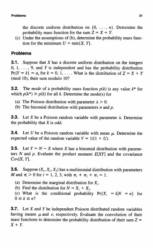
3.1. Suppose that X has a discrete uniform distribution on the integers0, 1, ... , 9, and Y is independent and has the probability distributionPr{Y = k} = ak for k = 0, 1, .... What is the distribution of Z = X + Y(mod 10), their sum modulo 10?
3.2. The mode of a probability mass function p(k) is any value k* forwhich p(k*) >_ p(k) for all k. Determine the mode(s) for
(a) The Poisson distribution with parameter A > 0.(b) The binomial distribution with parameters n and p.
3.3. Let X be a Poisson random variable with parameter A. Determinethe probability that X is odd.
3.4. Let U be a Poisson random variable with mean µ. Determine theexpected value of the random variable V = 1/(1 + U).
3.5. Let Y = N - X where X has a binomial distribution with parame-ters N and p. Evaluate the product moment E[XY] and the covarianceCov[X, Y].
3.6. Suppose (X,, X,, )(,) has a multinomial distribution with parametersM and ir, > 0 for i = 1, 2, 3, with 7r,+7r,+ir,= 1.
(a) Determine the marginal distribution for X,.(b) Find the distribution for N = X, + X,.(c) What is the conditional probability Pr{X1 = kIN = n} for0<_k--- n?
3.7. Let X and Y be independent Poisson distributed random variableshaving means µ and v, respectively. Evaluate the convolution of theirmass functions to determine the probability distribution of their sum Z =X+Y.

32 I Introduction
3.8. Let X and Y be independent binomial random variables having pa-rameters (N, p) and (M, p), respectively. Let Z = X + Y.
(a) Argue that Z has a binomial distribution with parameters (N + M, p)by writing X and Y as appropriate sums of Bernoulli random vari-ables.
(b) Validate the result in (a) by evaluating the necessary convolution.
3.9. Suppose that X and Y are independent random variables with thegeometric distribution
p(k) = (1 - ir)iTk for k = 0, 1, ... .
Perform the appropriate convolution to identify the distribution of Z = X+ Y as a negative binomial.
3.10. Determine numerical values to three decimal places forPr{X = k},k= 0, 1,2,when
(a) X has a binomial distribution with parameters n = 10 and p = 0.1.(b) X has a binomial distribution with parameters n = 100 and p =
0.01.(c) X has a Poisson distribution with parameter A = 1.
3.11. Let X and Y be independent random variables sharing the geo-metric distribution whose mass function is
p(k) = (1 - ir)irk for k = 0, 1, ... ,where 0<n<1.Let U=min{X,Y},V=max{X,Y}, and W = V - U.Determine the joint probability mass function for U and W and show thatU and W are independent.
3.12. Suppose that the telephone calls coming into a certain switch-board during a one-minute time interval follow a Poisson distribution withmean A = 4. If the switchboard can handle at most 6 calls per minute,what is the probability that the switchboard will receive more calls than itcan handle during a specified one-minute interval?
3.13. Suppose that a sample of 10 is taken from a day's output of a ma-chine that produces parts of which 5 percent are normally defective. If 100

4. Important Continuous Distributions 33
percent of a day's production is inspected whenever the sample of 10gives 2 or more defective parts, then what is the probability that 100 per-cent of a day's production will be inspected? What assumptions did youmake?
3.14. Suppose that a random variable Z has the geometric distribution
Pz(k) = p(1 - p)k for k = 0, 1, ... ,
where p = 0.10.
(a) Evaluate the mean and variance of Z.(b) What is the probability that Z strictly exceeds 10?
3.15. Suppose that X is a Poisson distributed random variable withmean A = 2. Determine Pr(X <- A).
3.16. Consider the generalized geometric distribution defined by
Pk = b(l - p)k for k = 1, 2, ... ,and
x
Po=1-7Pk,k=1
where 0 < p < 1 and p <- b <- p/(1 - p).
(a) Evaluate po in terms of b and p.(b) What does the generalized geometric distribution reduce to when
b=p?When b=pl(1 -p)?(c) Show that N = X + Z has the generalized geometric distribution
when X is a Bernoulli random variable for which Pr{X = 11 = a,0 < a < 1, and Z independently has the usual geometric distribu-tion given in (3.4).
4. Important Continuous Distributions
For future reference, this section catalogs several continuous distributionsand some of their properties.

34 I Introduction
4.1. The Normal Distribution
The normal distribution with parameters µ and o' > 0 is given by the fa-miliar bell-shaped probability density function
(, µ, ') = 1 e ,. µ, / 2?'Q- -x < x < x. (4.1)x ,
The density function is symmetric about the point F.c, and the parameter o'is the variance of the distribution. The case µ = 0 and o' = 1 is referredto as the standard normal distribution. If X is normally distributed withmean µ and variance o', then Z = (X - µ)/o- has a standard normal dis-tribution. By this means, probability statements about arbitrary normalrandom variables can be reduced to equivalent statements about standardnormal random variables. The standard normal density and distributionfunctions are given respectively by
b() = 1 e-F212 -oc < 6 < 00, (4.2)
and
c(x) = j (P(6) d6, -x < x < x. (4.3)
The central limit theorem explains in part the wide prevalence of thenormal distribution in nature. A simple form of this aptly named result con-cerns the partial sums S,, = , + + ,, of independent and identicallydistributed summands ,, 62, ... having finite means µ = E[&k] and finitevariances cr- = In this case, the central limit theorem asserts that
lim PrjS,,
7L x}=
I (x) for all x. (4.4)II- % I n
The precise statement of the theorem's conclusion is given by equation(4.4). Intuition is sometimes enhanced by the looser statement that, forlarge n, the sum S,, is approximately normally distributed with mean nµand variance no-'.
In practical terms we expect the normal distribution to arise wheneverthe numerical outcome of an experiment results from numerous small ad-ditive effects, all operating independently, and where no single or smallgroup of effects is dominant.

4. Important Continuous Distributions 35
The Lognormal Distribution
If the natural logarithm of a nonnegative random variable V is normallydistributed, then V is said to have a lognormal distribution. Conversely, ifX is normally distributed with mean µ and variance cr2, then V = e' de-fines a lognormally distributed random variable. The change-of-variableformula (2.15) applies to give the density function for V to be
1exp{-
1(ln v - µ )'J'v ? 0. (4.5)V ov 2 o, j
The mean and variance are, respectively,
E[V] = exp{µ + to },
Var[V] = exp{2(µ + 1].
4.2. The Exponential Distribution
(4.6)
A nonnegative random variable T is said to have an exponential distribu-tion with parameter A > 0 if the probability density function is
At
.fT(t) =(oe for t ? 0,
for t > 0. (4.7)
The corresponding distribution function is
FT(t) = 1 - e- At fort ? 0, (4.8){0 fort > 0,
and the mean and variance are given, respectively, by
1 1E[T] _ and Var[T] = ,.
Note that the parameter is the reciprocal of the mean and not the meanitself.
The exponential distribution is fundamental in the theory of continu-ous-time Markov chains (see V), due in major part to its memoryless prop-erty, as now explained. Think of T as a lifetime and, given that the unit

36 1 Introduction
has survived up to time t, ask for the conditional distribution of the re-maining life T - t. Equivalently, for x > 0 determine the conditionalprobability Pr{T - t > xIT > t}. Directly applying the definition of con-ditional probability (see Section 2.7), we obtain
Pr{T-t>xIT>t} = Pr{T>t+x,T>t}Pr{T > T}
Pr{T>t+x}(because x > 0) (4.9)
Pr{T > t}e-xcr+.
[from (4.8)]
There is no memory in the sense that Pr{T - t > xIT > t} = e-a` _Pr IT > x), and an item that has survived fort units of time has a remain-ing lifetime that is statistically the same as that for a new item.
To view the memoryless property somewhat differently, we introducethe hazard rate or failure rate r(s) associated with a nonnegative randomvariable S having continuous density g(s) and distribution function G(s) <1. The failure rate is defined by
r(s) =1 g(G(s)
for s > 0. (4.10)
We obtain the interpretation by calculating (see Section 2.2)
Pr{s<S5s+Osls<S} _ Pr{s<S:5 s+As)Pr{s < S}
+ o(As) [from (2.5)]g(s) As
1 - G(s)
= r(s) As + o(Os).
An item that has survived to time s will then fail in the interval (s, s + Os]with conditional probability r(s) As + o(1s), thus motivating the name"failure rate."
4. Important Continuous Distributions
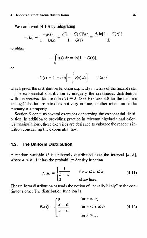
We can invert (4.10) by integrating
-g(s) _ d[ I - G(s)]Ids - d{ ln[ 1 - G(s)] }-r(s) =
1 - G(s) 1 - G(s) ds
to obtain
- f r(s) ds = In[ 1 - G(t)],0
or
G(t) = 1 -expj - f r(s) ds}, t ? 0,l 0
37
which gives the distribution function explicitly in terms of the hazard rate.The exponential distribution is uniquely the continuous distribution
with the constant failure rate r(t) = A. (See Exercise 4.8 for the discreteanalog.) The failure rate does not vary in time, another reflection of thememoryless property.
Section 5 contains several exercises concerning the exponential distri-bution. In addition to providing practice in relevant algebraic and calcu-lus manipulations, these exercises are designed to enhance the reader's in-tuition concerning the exponential law.
4.3. The Uniform Distribution
A random variable U is uniformly distributed over the interval [a, b],where a < b, if it has the probability density function
1
fi (u) = b - a for a --- u :5 b,
0 elsewhere.
(4.11)
The uniform distribution extends the notion of "equally likely" to the con-tinuous case. The distribution function is
10 for a a,
(x)= x-a for a<x:! b, (4.12)b - a1 for x > b,

38 I Introduction
and the mean and variance are, respectively,
E[U] = 2 (a + b) and Var[U] _ (b12a)'
The uniform distribution on the unit interval [0, 1], for which a = 0 andb = 1, is most prevalent.
4.4. The Gamma Distribution
The gamma distribution with parameters a > 0 and A > 0 has probabilitydensity function
f(x) = rA (Ax)"-'e-' for x > 0. (4.13)
Given an integer number a of independent exponentially distributed ran-dom variables Y,, ... , Ya having common parameter A, then their sumXX = Y, + + Y. has the gamma density of (4.13), from which we ob-tain the moments
E[Xa] = Ci and Var[Xa] = z
these moment formulas holding for noninteger a as well.
4.5. The Beta Distribution
The beta density with parameters a > 0 and /3 > 0 is given by
f( x) + J3)
x) F(a)r(R)x«- x)a- I for0<x<1,
(4.14)
0 elsewhere.
The mean and variance are, respectively,
E[X] =a
aand Var[X] = (a + al+ + 1
(The gamma and beta functions are defined and briefly discussed in Sec-tion 6.)
4. Important Continuous Distributions 39
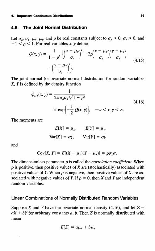
4.6. The Joint Normal Distribution
Let ox, o-v, lxx, Ar, and p be real constants subject to ox > 0, o,. > 0, and-1 < p < 1. For real variables x, y define
1
f(X - x)2 - --µY)
(4.15))2}
+ (Y
The joint normal (or bivariate normal) distribution for random variablesX, Y is defined by the density function
ik(x ) =1
x. v 1J27roxo, 1 --p2
The moments are
and
x exp{- 2 Q(x, Y)}, - 00 < x, Y < 00.
E[X]=µx, E[Y]=p,
Var[X] = oil, Var[Y] = Cry.
(4.16)
Cov[X, Y] = E[(X - µx)(Y - Ay)] = poxor
The dimensionless parameter p is called the correlation coefficient. Whenp is positive, then positive values of X are (stochastically) associated withpositive values of Y. When p is negative, then positive values of X are as-sociated with negative values of Y. If p = 0, then X and Y are independentrandom variables.
Linear Combinations of Normally Distributed Random Variables
Suppose X and Y have the bivariate normal density (4.16), and let Z =aX + by for arbitrary constants a, b. Then Z is normally distributed withmean
E[Z] = aµx + bµ}
40 I Introduction
and variance
Var[X] = a2oX + 2abpoxo + b2oy.
A random vector X...... X,,, is said to have a multivariate normal dis-tribution, or a joint normal distribution, if every linear combinationa,X, + + a univariate normal distribution. Obvi-ously, if X,..... X has a joint normal distribution, then so does the ran-dom vector Y ... , Y,,,, defined by the linear transformation in which
forj= 1,...,m,
for arbitrary constants a;;.
Exercises
4.1. The lifetime, in years, of a certain class of light bulbs has an expo-nential distribution with parameter A = 2. What is the probability that abulb selected at random from this class will last more than 1.5 years?What is the probability that a bulb selected at random will last exactly 1.5years?
4.2. The median of a random variable X is any value a for whichPr{X s a} >_
2
and Pr{X ? a) ? Z. Determine the median of an exponen-tially distributed random variable with parameter A. Compare the medianto the mean.
4.3. The lengths, in inches, of cotton fibers used in a certain mill are ex-ponentially distributed random variables with parameter A. It is decided toconvert all measurements in this mill to the metric system. Describe theprobability distribution of the length, in centimeters, of cotton fibers inthis mill.
4.4. Twelve independent random variables, each uniformly distributedover the interval (0, 1], are added, and 6 is subtracted from the total. De-termine the mean and variance of the resulting random variable.
4.5. Let X and Y have the joint normal distribution described in equa-tion (4.16). What value of a minimizes the variance of Z = aX +(1 - a)Y? Simplify your result when X and Y are independent.

Problems 41
4.6. Suppose that U has a uniform distribution on the interval [0, 1]. De-rive the density function for the random variables
(a) Y = -ln(1 - U).(b) W,, = U" for n > 1.
Hint: Refer to Section 2.6.
4.7. Given independent exponentially distributed random variables Sand T with common parameter A, determine the probability density func-tion of the sum R = S + T and identify its type by name.
4.8. Let Z be a random variable with the geometric probability massfunction
p(k) = (1 - ir)#rk, k = 0, 1, ... ,where 0 < ?r < 1.
(a) Show that Z has a constant failure rate in the sense thatPr{Z=kIZ?k}=1- 7r fork=0,1,....
(b) Suppose Z' is a discrete random variable whose possible valuesare 0, 1, .... and for which Pr (Z' = kIZ' ? k} = 1 - 7r fork = 0, 1, .... Show that the probability mass function for Z' is p(k).
Problems
4.1. Evaluate the moment E[e '], where A is an arbitrary real numberand Z is a random variable following a standard normal distribution, byintegrating
11-e 212 dz.
Hint: Complete the square -Z z2 + Az = -[(z - A)2 - A2] and usethe fact that
r I e-(z -a)-/2 dz = 1.
4.2. Let W be an exponentially distributed random variable with para-meter 0 and mean p. = 1/0.
(a) Determine Pr{ W > p.).(b) What is the mode of the distribution?
42 I Introduction
4.3. Let X and Y be independent random variables uniformly distributedover the interval [6 -Z, 0 + Z] for some fixed 0. Show that W = X - Yhasa distribution that is independent of 0 with density function
1+w for-law<0,fw(w)= 1-w for0 w<1,
10 forlwl> 1.
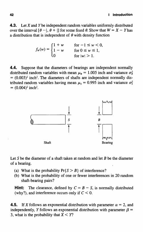
4.4. Suppose that the diameters of bearings are independent normallydistributed random variables with mean µ$ = 1.005 inch and variance o= (0.003)2 inch2. The diameters of shafts are independent normally dis-tributed random variables having mean µs = 0.995 inch and variance os= (0.004)2 inch2.
w
6
Shaft Bearing
Let S be the diameter of a shaft taken at random and let B be the diameterof a bearing.
(a) What is the probability Pr(S > B) of interference?(b) What is the probability of one or fewer interferences in 20 random
shaft-bearing pairs?
Hint: The clearance, defined by C = B - S, is normally distributed(why?), and interference occurs only if C < 0.
4.5. If X follows an exponential distribution with parameter a = 2, andindependently, Y follows an exponential distribution with parameter 8 =3, what is the probability that X < Y?

5. Some Elementary Exercises 43
5. Some Elementary Exercises
We have collected in this section a number of exercises that go beyondwhat is usually covered in a first course in probability.
5.1. Tail Probabilities
In mathematics, what is a "trick" upon first encounter becomes a basictool when familiarity through use is established. In dealing with nonneg-ative random variables, we can often simplify the analysis by the trick ofapproaching the problem through the upper tail probabilities of the formPr{X > x}. Consider the following example.
A jar has n chips numbered 1, 2, . . . , n. A person draws a chip, returnsit, draws another, returns it, and so on, until a chip is drawn that has beendrawn before. Let X be the number of drawings. Find the probability dis-tribution for X.
It is easier to compute Pr{X > k} first. Then, Pr{X > 1 } = 1, since atleast two draws are always required. The event (X > 2) occurs when dis-
_tinct numbers appear on the first two draws, whence Pr{X > 2)(nln)[(n - 1)/n]. Continuing in this manner, we obtain
Pr(X>k)=1(1-n)(1 )n...(1-kn1/ fork= 1,...,n- 1. (5.1)
Finally,
Pr{X = k} = Pr{X > k - 1) - Pr{X > k}
=r(1_n)...(1kn2)J
_L(1_n)...(1kn2)\1
kn1)1
_(1 n)...(1_kn2)L1-(1kn1)J
nkn1(1_n)...(1- k 2
fork=2,...,n+ 1.

44 1 Introduction
Now try deriving Pr(X = k) directly, for comparison with the "trick"approach.
The usefulness of the upper tail probabilities is enhanced by the formulax x
E[X] _ 7, Pr{X > k} = 7, Pr{X ? k}, (5.2)k=0 k=1
valid for nonnegative integer-valued random variables X. To establish(5.2), abbreviate the notation by using p(k) = Pr{X = k}, and rearrangethe terms in E[X] = E,z, kp(k) as follows:
E[X] = Op(O) + lp(l) + 2p(2) + 3p(3) +
=p(1)+p(2)+p(3)+p(4)++ p(2) + p(3) + p(4) +
+p(3)+p(4)++p(4)+
=Pr{X? 1)+Pr{X?2}+Pr{X? 3}+
k=1
Pr{X ? k},
thus establishing (5.2).For the chip drawing problem, the mean number of draws required,
then, is
E[X] = Pr{X > 0} + Pr{X > 11 + + Pr{X > n},
since Pr{X > k) = 0 fork > n. Then substituting (5.1) into (5.2) leads di-rectly to
E[X]=2+(1-1) +(1 n)(l n)
+...
+ 1 nl(1 n) ... (1 - nn 1).
Now let X be a nonnegative continuous random variable with densityf(x)and distribution function F(x). The analog to (5.2) is
E[X] f [I - F(z)] dz, (5.3)n
5. Some Elementary Exercises 45
obtained by interchanging an order of integration as follows:
E[X] = J xf(x) dx f (J dz)f(x) dx
= dx]dz= J [I -F(z)]dzr[if(X)x
Interchanging the order of integration where the limits are variablesoften proves difficult for many students. The trick of using indicator func-tions to make the limits of integration constant may simplify matters. Inthe preceding interchange, let
1(z < x) =11 if 0<-z<x,to otherwise,
and then
1[J dz]f(x) dx = J [ J 1(z < x)f(x) dz] dx
x x x x
f [ f 1(z < x)f(x) dx] dz = J [f f(x) dx] dz.
As an application of (5.3), let XX = min (c, X) for some positive con-stant c. For example, suppose X is the failure time of a certain piece ofequipment. A planned replacement policy is put in use that calls for re-placement of the equipment upon its failure or upon its reaching age c,whichever occurs first. Then
X, =min(c, X) =X if X -- c,
{c ifX>cis the time for replacement.Now
Pr{X,>z}_11-F(z)
if05 z,
G <c,whence we obtain
E[Xc] = J [1 - F(z)] dz,0

46 1 Introduction
which is decidedly shorter than
E[XX] = J xf(x) dx + c[1 - F(c)].0
Observe that X, is a random variable whose distribution is partly con-tinuous and partly discrete, thus establishing by example that such distri-butions do occur in practical applications.
5.2. The Exponential Distribution
This exercise is designed to foster intuition about the exponential distrib-ution, as well as to provide practice in algebraic and calculus manipula-tions relevant to stochastic modeling.
Let X0 and X, be independent exponentially distributed random vari-ables with respective parameters A0 and A,, so that
Pr{X;>t}=e-A,` fort?O,i=0,1.Let
and
_ 0 ifX0-XN-{1if X, X0,
U = min{X0, X, } = XN;
M 1 - N;
V = max{X0, X,} = XM;
W=V-U=jX0-X,j.In this context, we derive the following:
(a) Pr(N = 0 and U > t} = e-cAo )tA0(a0+ A, ).
The event (N = 0 and U > t } is exactly the event { t < X0 < X, }, whence
Pr{N = 0, U > t} = Pr{t < X0 < X, j
= f f A0e-AoxoA,e-Aix1 dx, dx0
Kxp<x,

5. Some Elementary Exercises 47
= f (rAie'x' )A0e_A0x0o
+ xo
=fe
A0J
(AO + A,)e-(,+A,)r0
dx0A0+A,,
= A0 e (AO+A
AO + A,
(b) Pr{N = 0 } =Ao
+oA,
and Pr{N = 1) = AO +' A, .
We use the result in (a) as follows:
Pr{N = 0) = Pr{N = 0, U > 0) = A0 from (a).AO + A,
Obviously, Pr{N = 1) = 1 - Pr{N = 0) = A,/(AO + A,).
(c) Pr{ U > t} = e (AO+a,'', t ? 0.
Upon adding the result in (a),
+A1
" A0,,(,Pr{N = 0 and U > t} = e
A0 +A,,
to the corresponding quantity associated with N = 1,
Pr{N = I and U > t} = e-('t) +A,),A
A + A 'o )
we obtain the desired result via
Pr{ U > t} = Pr{N = 0, U > t} + Pr{N = 1, U > t}
= e-cAO+A,"Ao +
A,
IAO+A, A0+A,e-(A+A,),

48 I Introduction
At this point observe that U and N are independent random variables.This follows because (a), (b), and (c) together give
Pr{N = 0 and U > t} = Pr{N = 0} X Pr{ U > t}.
Think about this remarkable result for a moment. Suppose X0 and X,represent lifetimes, and A0 = 0.001, while A, = 1. The mean lifetimes areE[Xo] = 1000 and E[X,] = 1. Suppose we observe that the time of the firstdeath is rather small, say, U = min{Xo, X, } = z. In spite of vast disparitybetween the mean lifetimes, the observation that U = 2 provides no infor-mation about which of the two units, 0 or 1, was first to die! This appar-ent paradox is yet another, more subtle, manifestation of the memorylessproperty unique to the exponential density.
We continue with the exercise.
(d) Pr{W>tIN=0} =e-A", t?0.
The event { W > t and N = 0) for t ? 0 corresponds exactly to theevent It < X, - X0). Thus
Pr{W> tandN= 0} = Pr{X, - Xo> t}
I JAoe AOXoA,e
A'x'dxo dx,
X, -Xo>r
= J ( f A,e A'x' dx )Aoe °x° dxo0 Xo+r
(= J e-A,(Xo+n Aoe-A,yo dX0
0
e-r(0 + A,)e-(,k.+A, o dxoAo + A, 0
= Ao
A0 + A,
= Pr{N = 0}e-A,` [from (b)].

5. Some Elementary Exercises 49
Then, using the basic definition of conditional probability (Section 2.7),we obtain
Pr{W>tIN=O} = Pr{W>t,N=0} =e-Ai', t?0,Pr{N = 0}
as desired.Of course a parallel formula holds conditional on N = 1:
Pr{W>tIN= 1} =e-/, t?0,and using the law of total probability we obtain the distribution of W inthe form
Pr{W>t} =Pr{W>t,N=O} +Pr{W>t,N= 1}
AO A
-a r
-Aor
t> 0
e , +AO
,+ A0 + )
(e) U and W = V - U are independent random variables.
To establish this final consequence of the memoryless property, it suf-fices to show that
Pr{U>uand W> w) =Pr{U>u} Pr{W>w} forall u ?0, w ?0.
Determining first
Pr{N=0, U>u,W>w} =Pr{u<X0<X, -w)
= f r o I
u<xo<x, -w
=J J Ale-"l x I dr,)A0e-Aoxo droU xo+w
_ f e-A,(x(-+w) 1We-Aox-
u
,
AO -A,w-(Ap+A,)e,
(A0 +)e e
)e-A,u I (A0 + A')e-cAo+A,Iro Xo_ (A oA
50 1 Introduction
and then, by symmetry,
and finally adding the two expressions, we obtain
Pr( U > u, W > w} =Rko
t )e-","+
(+' 1lo + AO
=Pr{W>w}Pr{U>u}, u,w?0.The calculation is complete.
Exercises
5.1. Let X have a binomial distribution with parameters n = 4 and p = ;.Compute the probabilities Pr{X ? k} for k = 1, 2, 3, 4, and sum these toverify that the mean of the distribution is 1.
5.2. Ajar has four chips colored red, green, blue, and yellow. A persondraws a chip, observes its color, and returns it. Chips are now drawn re-peatedly, without replacement, until the first chip drawn is selected again.What is the mean number of draws required?
5.3. Let X be an exponentially distributed random variable with para-meter A. Determine the mean of X
(a) by integrating by parts in the definition in equation (2.7) withm =1
(b) by integrating the upper tail probabilities in accordance with equa-tion (5.3).
Which method do you find easier?
5.4. A system has two components: A and B. The operating times untilfailure of the two components are independent and exponentially distrib-uted random variables with parameters 2 for component A, and 3 for B.The system fails at the first component failure.
(a) What is the mean time to failure for component A? For componentB?

Problems 51
(b) What is the mean time to system failure?(c) What is the probability that it is component A that causes system
failure?(d) Suppose that it is component A that fails first. What is the mean re-
maining operating life of component B?
5.5. Consider a post office with two clerks. John, Paul, and Naomi entersimultaneously. John and Paul go directly to the clerks, while Naomi mustwait until either John or Paul is finished before she begins service.
(a) If all of the service times are independent exponentially distributedrandom variables with the same mean 1/A, what is the probabilitythat Naomi is still in the post office after the other two have left?
(b) How does your answer change if the two clerks have different ser-vice rates, say A, = 3 and A, = 47?
(c) The mean time that Naomi spends in the post office is less than thatfor John or Paul provided that max { A A2) > c min( A, , A, j for acertain constant c. What is the value of this constant?
Problems
5.1. Let X, , X2, ... be independent and identically distributed randomvariables having the cumulative distribution function F(x) = Pr{X < x}.For a fixed number , let N be the first index k for which Xk > . That is,N = 1 if X, > 6; N = 2 if X, < and X, > ; etc. Determine the proba-bility mass function for N.
5.2. Let X X,, ... , X,, be independent random variables, all exponen-tially distributed with the same parameter A. Determine the distributionfunction for the minimum Z = min{X......
X is a discrete random variable having the geometricdistribution whose probability mass function is
p(k) = p(1 - p)k for k = 0, 1, ... .
(a) Determine the upper tail probabilities Pr{X > k} for k = 0, 1, ... .(b) Evaluate the mean via E[X] = Ek>o Pr{X > k }.

52 I Introduction
5.4. Let V be a continuous random variable taking both positive andnegative values and whose mean exists. Derive the formula
0
E[V] = J [1 - F,,(v)] dv - J F,(v) dv.0 -x
5.5. Show that
E[W2] = J 2y[I - F,,,(y)] dy0
for a nonnegative random variable W.
5.6. Determine the upper tail probabilities Pr{V > t} and mean E[V]for a random variable V having the exponential density
I- for v < 0,f'-(v) _ A, for v ? 0,
where A is a fixed positive parameter.
5.7. Let X,, X,, ... , X,, be independent random variables that are expo-nentially distributed with respective parameters A A...... A,,. Identifythe distribution of the minimum V = min (X,, X,, .. . ,
Hint: For any real number v, the event ( V > v) is equivalent to
5.8. Let U,, U,, ... , U be independent uniformly distributed randomvariables on the unit interval [0, 1]. Define the minimum V _min{U U,, ... ,
(a) Show that Pr { V,, > v } = (1 - v)" for 0 : v <_ 1.(b) Let W = nV,,,. Show that Pr { W > w) 1 - (w/n)]" for 0 <- w n,
and thus
w} = e- forw?0.
5.9. A flashlight requires two good batteries in order to shine. Suppose,for the sake of this academic exercise, that the lifetimes of batteries in use

6. Useful Functions, Integrals, and Sums 53
are independent random variables that are exponentially distributed withparameter h = 1. Reserve batteries do not deteriorate. You begin with fivefresh batteries. On average, how long can you shine your light?
6. Useful Functions, Integrals, and Sums
Collected here for later reference are some calculations and formulas thatare especially pertinent in probability modeling.
We begin with several exponential integrals, the first and simplest being
f ex dx = -e-x. (6.1)
When we use integration by parts, the second integral that we introducereduces to the first in the manner
f xe-x dx = -xe-x + J ex dx = -e-x(1 + x). (6.2)
Then (6.1) and (6.2) are the special cases of a = 1 and a = 2, respec-tively, in the general formula, valid for any real number a for which theintegrals are defined, given by
J x°-'e-.,. dx = -x°-'e-x + (a - 1) J x°-2e-x dx. (6.3)
Fixing the limits of integration leads to the gamma function, defined by
I'(a) = J xa-'e-x dx, for a > 0. (6.4)0
From (6.3) it follows that
['(a) = (a - 1)1'(a- 1), (6.5)
and therefore, for any integers k,
I'(k) _ (k - 1)(k - 2) 2 I'(1). (6.6)

54 I Introduction
An easy consequence of (6.1) is the evaluation I'(1) = 1, which with (6.5)shows that the gamma function at integral arguments is a generalizationof the factorial function, and
IF(k) = (k - 1)! for k = 1, 2, .... (6.7)
A more difficult integration shows that
I'() = V, (6.8)
which with (6.6) provides
I(n+;)= forn=0,1..... (6.9)
Stirling's formula is the following important asymptotic evaluation ofthe factorial function:
n! = n"e-"(2irn)1/2er(n)112", (6.10)
in which
1 12n+ 1< r(n) < 1.
We sometimes write this in the looser form
(6.11)
n! - n"e-"(27m)1/2 as n - oo, (6.12)
the symbol "-" signifying that the ratio of the two sides in (6.12) ap-proaches 1 as n - oo. For the binomial coefficient (k) = n!/[k!(n - k)!] wethen obtain
(n\ (n - k)k
k) k!as n*c, (6.13)
as a consequence of (6.12) and the exponential limit
"e-k = Jim (1 -
kk .
pl-. n
The integral
B(m, n) = f x"'-'(1 - x)"-' dx, (6.14)0

6. Useful Functions, Integrals, and Sums 55
which converges when m and n are positive, defines the beta function, re-lated to the gamma function by
B(m, nr(m)r(n)
form > 0, n > 0. (6.15))= r(m+n)For nonnegative integral values m, n,
B(m+1,n+1)= f x(1-x)"dx= m!n!
(m + n + 1)! '(6.16)
For n = 1, 2, ... , the binomial theorem provides the evaluation
(1 - x)" _ (-1)"(n)xk, for -oo < x < oo. (6.17)k=0 k
The formula may be generalized for nonintegral n by appropriately gen-eralizing the binomial coefficient, defining for any real number a,
1a(a- 1) (a-k+ 1)_ k! for k = 1, 2, ... , (6.18)
(Ok')1 fork = 0.
As a special case, for any positive integer n,
r n) (-1)k n(n + (n + k - 1)\k k!
n + k - 1= (-1)k(k )
The general binomial theorem, valid for all real a, is
k=0
-1)k(k)xk
(6.19)
for -1 < x < 1. (6.20)
When a = -n for a positive integer n, we obtain a group of formulas use-ful in dealing with geometric series. For a positive integer n, in view of(6.19) and (6.20), we have
(- 1)(1 - x) " = n + k xkfor jxj < 1. (6.21)
k=0 k

56 I Introduction
The familiar formula
17, xk = 1 + x + x2 + = for jxl < 1 (6.22)k=O 1 - x
for the sum of a geometric series results from (6.21) with n = 1. The casesn = 2 and n = 3 yield the formulas
x7- (k+ 1)xk= I +2x+3x2+...k=0
1 for l < 1 23)(6(1 -x)22
, .
2k + 2 k + 1 k = l <f 6 247 ( )( )x
3
or Ix 1. ( . )(1k=O - x)
Sums of Numbers
The following sums of powers of integers have simple expressions:
n(n + 1)
2 '
n(n + 1)(2n + 1)
6
n22(n + 1)2
4

Chapter IIConditional Probability and
Conditional Expectation
1. The Discrete Case
The conditional probability Pr{AJB} of the event A given the event B isdefined by
Pr{A1B} =Pr{A and B}
if Pr{B} > 0, (1.1)Pr{B)
and is not defined, or is assigned an arbitrary value, when Pr{B} = 0. LetX and Y be random variables that can attain only countably many differ-ent values, say 0, 1, 2, .... The conditional probability mass functionpxr(xl y) of X given Y = y is defined by
Pr{X=xand Y=y}Pxr(xl y) = Pr{ Y = y}
if Pr{ Y = y} > 0,
and is not defined, or is assigned an arbitrary value, wheneverPr{ Y = y} = 0. In terms of the joint and marginal probability mass func-tions pxr(x, y) and py(y) = E, pxr(x, y), respectively, the definition is
Pxr(xlY) =Pxt(x> y)
pr(y)if pr(y) > 0; x, y = 0, 1..... (1.2)
Observe that pxr(xl y) is a probability mass function in x for each fixedy, i.e., pxr(xl y) ? 0 and If px r(6l y) = 1, for all x, y.

58 II Conditional Probability and Conditional Expectation
The law of total probability takes the formY_
Pr{X = x) _ I Px r(xIY)Pv(Y) (1.3)
Notice in (1.3) that the points y where px y(xl y) is not defined are exactlythose values for which p.(y) = 0, and hence, do not affect the computa-tion. The lack of a complete prescription for the conditional probabilitymass function, a nuisance in some instances, is always consistent withsubsequent calculations.
Example Let X have a binomial distribution with parameters p and N,where N has a binomial distribution with parameters q and M. What is themarginal distribution of X?
We are given the conditional probability mass function
pxrc(kln) = ()p(1 - p),,-k,
and the marginal distribution
k=0, 1.... ,n,
pN(n) =(M)q, (1 - q)", n = 0, 1, ... , M.
n
We apply the law of total probability in the form of (1.3) to obtain
M
Pr{X = k} = 7, px,(kI n)p,(n)=0
M 12!
k!(n - k)!px (1 - p)"-k
X(1gq
M! q"(1 - q)M
n!(M - n)!
- k)!(M - n)! (1 -1
= M! (pq)"(1 _ q),ti, x(1 + q(1 p)1M-k
k!(M-k)! L 1 -q J

1. The Discrete Case 59
M!= k!(M - k)! (pq)k(1 - pq)M-k, k = 0, 1, ... , M.
In words, X has a binomial distribution with parameters M and pq.
Example Suppose X has a binomial distribution with parameters p andN where N has a Poisson distribution with mean A. What is the marginaldistribution for X?
Proceeding as in the previous example but now usingAue-A
PN(n)= , n=0,1,...,n!
we obtain
Pr{X = k} = > PXN(kjn)pN(n),r=0
n ! A"e -Ak(1 - rr kn_k k!(n _ k)! P p)
n!
Ake-Apk . [A(1p)],,-k
k! =k (n - k)!
(Ap)k e--'A(] -p)
k!
(AP)ke-A,,
k!fork = 0, 1, ... .
In words, X has a Poisson distribution with mean Ap.
Example Suppose X has a negative binomial distribution with parame-ters p and N, where N has the geometric distribution
Pv(n) _ (1 - for n = 1, 2, ... .
What is the marginal distribution for X?We are given the conditional probability mass function
n+k-1 7
pxN(kl n) = ( k)prr(1 - p)k, k = 0, 1 , ... .

60 II Conditional Probability and Conditional Expectation
Using the law of total probability, we obtainx
Pr{X = k} = 7 pXN(kln)pN(n)n=o
n=
(n + k - 1)!P)k(l - P)le»-]
k!(n - 1)!
(1 - MO - P)kPn k
> ( knl= (1 - J3)(1 - P)*P(l - 8p)-k-I
(pQI
- P kfork = 0, 1, ... .)- 05 lGP
We recognize the marginal distribution of X as being of geometric form.
Let g be a function for which the expectation of g(X) is finite. We de-fine the conditional expected value of g(X) given Y = y by the formula
E[g(X )I Y = y] = 7 g(x)Pr(xly) if Pr(y) > 0, (1.4)
and the conditional mean is not defined at values y for which py(y) = 0.The law of total probability for conditional expectation reads
E[g(X )] = 7 E[g(X )I Y = y]Pr(y). (1.5)Y
The conditional expected value E[g(X)IY = y] is a function of the realvariable y. If we evaluate this function at the random variable Y, we ob-tain a random variable that we denote by E[g(X )I Y]. The law of total prob-ability in (1.5) now may be written in the form
E[g(X)] = (1.6)
Since the conditional expectation of g(X) given Y = y is the expectationwith respect to the conditional probability mass function pxr(xl y), condi-tional expectations behave in many ways like ordinary expectations. Thefollowing list summarizes some properties of conditional expectations. In

Exercises 61
this list, with or without affixes, X and Y are jointly distributed randomvariables; c is a real number; g is a function for which E[Ig(X)I] < CO ; his a bounded function; and v is a function of two variables for whichE[Iv(X, Y)I ] < oo. The properties are
(1) E[c,g,(X,) + c2g2(X2)IY = y]
= cIE[gi(X1)IY = y] + c,E[g,(X,)I Y = y]. (1.7)
(2) if g?0, then E[g(X)IY = y] ?0. (1.8)
(3) E[v(X, Y)I Y = y] = E[v(X, y)IY = y]. (1.9)
(4) E[g(X)I Y = y] = E[g(X)] if X and Y are independent. (1.10)
(5) E[g(X)h(Y)I Y = y] = h(y)E[g(X )I Y = y]. (1.11)
(6) E[g(X)h(Y)j = I h(y)E[g(X )I Y = y]pr(y)Y (1.12)
= E{h(Y)E[g(X)IY]}.
As a consequence of (1.7), (1.11), and (1.12), with either g = 1 or h ° 1,we obtain
E[cI Y = y] = c, (1.13)
E[h(Y)I Y = y] = h(y), (1.14)
E[g(X)] = 7, E[g(X)I Y = y]pr(y) = E{E[g(X)IY]}.Y
(1.15)
Exercises
1.1. 1 roll a six-sided die and observe the number N on the uppermostface. I then toss a fair coin N times and observe X, the total number ofheads to appear. What is the probability that N = 3 and X = 2? What isthe probability that X = 5? What is E[X], the expected number of headsto appear?
1.2. Four nickels and six dimes are tossed, and the total number N ofheads is observed. If N = 4, what is the conditional probability that ex-actly two of the nickels were heads?

62 Ii Conditional Probability and Conditional Expectation
1.3. A poker hand of five cards is dealt from a normal deck of 52 cards.Let X be the number of aces in the hand. Determine Pr{X > lix ? 1).This is the probability that the hand contains more than one ace, given thatit has at least one ace. Compare this with the probability that the hand con-tains more than one ace, given that it contains the ace of spades.
1.4. A six-sided die is rolled, and the number N on the uppermost faceis recorded. From ajar containing 10 tags numbered 1 , 2, ... , 10 we thenselect N tags at random without replacement. Let X be the smallest num-ber on the drawn tags. Determine Pr(X = 2}.
1.5. Let X be a Poisson random variable with parameter A. Find the con-ditional mean of X given that X is odd.
1.6. Suppose U and V are independent and follow the geometric distri-bution
p(k) = p(1 - p)k fork = 0, 1, ... .
Define the random variable Z = U + V.
(a) Determine the joint probability mass function pU,Z(u, z) _Pr{U=u,Z=z}.
(b) Determine the conditional probability mass function for U giventhat Z = n.
Problems
1.1. Let M have a binomial distribution with parameters N and p. Con-ditioned on M, the random variable X has a binomial distribution with pa-rameters M and ir.
(a) Determine the marginal distribution for X.(b) Determine the covariance between X and Y = M - X.
1.2. A card is picked at random from N cards labeled 1, 2, ... , N, andthe number that appears is X. A second card is picked at random fromcards numbered 1, 2, ... , X and its number is Y. Determine the condi-tional distribution of X given Y = y, for y = 1, 2. ... .

Problems 63
1.3. Let X and Y denote the respective outcomes when two fair dice arethrown. Let U = min(X, Y}, V = max{X, Y}, and S = U + V, T = V - U.
(a) Determine the conditional probability mass function for U givenV=v.
(b) Determine the joint mass function for S and T.
1.4. Suppose that X has a binomial distribution with parameters p =and N, where N is also random and follows a binomial distribution withparameters q = ; and M = 20. What is the mean of X?
1.5. A nickel is tossed 20 times in succession. Every time that the nickelcomes up heads, a dime is tossed. Let X count the number of heads ap-pearing on tosses of the dime. Determine Pr{X = 0).
1.6. A dime is tossed repeatedly until a head appears. Let N be the trialnumber on which this first head occurs. Then a nickel is tossed N times.Let X count the number of times that the nickel comes up tails. DeterminePr{X = 0), Pr{X = 11, and E[X].
1.7. The probability that an airplane accident that is due to structuralfailure is correctly diagnosed is 0.85, and the probability that an airplaneaccident that is not due to structural failure is incorrectly diagnosed asbeing due to structural failure is 0.35. If 30 percent of all airplane acci-dents are due to structural failure, then find the probability that an airplaneaccident is due to structural failure given that it has been diagnosed as dueto structural failure.
1.8. Initially an urn contains one red and one green ball. A ball is drawnat random from the urn, observed, and then replaced. If this ball is red,then an additional red ball is placed in the urn. If the ball is green, then agreen ball is added. A second ball is drawn. Find the conditional proba-bility that the first ball was red given that the second ball drawn was red.
1.9. Let N have a Poisson distribution with parameter A = 1. Con-ditioned on N = n, let X have a uniform distribution over the integers0, 1, ... , n+ 1. What is the marginal distribution for X?
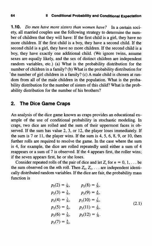
64 11 Conditional Probability and Conditional Expectation
1.10. Do men have more sisters than women have? In a certain soci-ety, all married couples use the following strategy to determine the num-ber of children that they will have: If the first child is a girl, they have nomore children. If the first child is a boy, they have a second child. If thesecond child is a girl, they have no more children. If the second child is aboy, they have exactly one additional child. (We ignore twins, assumesexes are equally likely, and the sex of distinct children are independentrandom variables, etc.) (a) What is the probability distribution for thenumber of children in a family? (b) What is the probability distribution for
'the number of girl children in a family? (c) A male child is chosen at ran-dom from all of the male children in the population. What is the proba-bility distribution for the number of sisters of this child? What is the prob-ability distribution for the number of his brothers?
2. The Dice Game Craps
An analysis of the dice game known as craps provides an educational ex-ample of the use of conditional probability in stochastic modeling. Incraps, two dice are rolled and the sum of their uppermost faces is ob-served. If the sum has value 2, 3, or 12, the player loses immediately. Ifthe sum is 7 or 11, the player wins. If the sum is 4, 5, 6, 8, 9, or 10, thenfurther rolls are required to resolve the game. In the case where the sumis 4, for example, the dice are rolled repeatedly until either a sum of 4reappears or a sum of 7 is observed. If the 4 appears first, the roller wins;if the seven appears first, he or she loses.
Consider repeated rolls of the pair of dice and let Z,, for n = 0, 1.... bethe sum observed on the nth roll. Then Z0, Z,, . . . are independent identi-cally distributed random variables. If the dice are fair, the probability massfunction is
Pz(2) = 36, Pz(8) = b,
Pz(3) = 36, Pz(9) = 6,
Pz(4) = 36, Pz(10) = 6
Pz(5) = 6, Pz(11) = 6
Pz(6) = 36, Pz(12) = 36
Pz(7) 36,
(2.1)

2. The Dice Game Craps 65
Let A denote the event that the player wins the game. By the law of totalprobability,
12
Pr{A} _ 7, Pr{AIZo = k}pz(k). (2.2)k=2
Because Zo = 2, 3, or 12 calls for an immediate loss, thenPr{AIZ0 = k) = 0 for k = 2, 3, or 12. Similarly, Zo = 7 or 11 results in animmediate win, and thus Pr(Alto = 7) = Pr{AIZ4 = 111 = 1. It remainsto consider the values 4 = 4, 5, 6, 8, 9, and 10, which call for additionalrolls. Since the logic remains the same in each of these cases, we willargue only the case in which Zo = 4. Abbreviate with a = Pr{AI4 = 4}.Then a is the probability that in successive rolls Z,, Z2, ... of a pair ofdice, a sum of 4 appears before a sum of 7. Denote this event by B, andagain bring in the law of total probability. Then
12
a = Pr{B} = I Pr{BIZ1 = k}pz(k). (2.3)k=2
Now Pr{BIZ, = 4) = 1, while Pr(BIZ, = 7) = 0. If the first roll results inanything other than a 4 or a 7, the problem is repeated in a statisticallyidentical setting. That is, Pr{BIZ1 = k} = a for k # 4 or 7. Substitutioninto (2.3) results in
a=pz(4)X1+pz(7)X0+ pz(k)Xak#4,7
= pz(4) + [1 - pz(4) - pz(7)]a,
or
pz(4)a =
pz(4) + pz(7)(2.4)
The same result may be secured by means of a longer, more computa-tional, method. One may partition the event B into disjoint elementalevents by writing
B= {Z, =4} U {Z, 04or7,Z2=4}
U {Z, 0 4 or 7,Z2* 4 or 7, Z., =4) U -

66 II Conditional Probability and Conditional Expectation
and then
Pr{B} = Pr{Z1 = 4} + Pr{Z1 * 4 or 7, Z, = 4}
+Pr{Z1 04 or7,Z,04or7,Z3=4}
Now use the independence of Z,, Z,, ... and sum a geometric series to se-cure
Pr{B} = pz(4) + [1 - pz(4) - pz(7)]pz(4)
+ [1 - pz(4) - pz(7)]2pz(4) + ...
pz(4)
pz(4) + pz(7)
in agreement with (2.4).Extending the result just obtained to the other cases having more than
one roll, we have
Pr{AIZ0=k} = pz(k) fork=4,5,6,8,9, 10.pz(k) + pz(7)
Finally, substitution into (2.2) yields the total win probability
Pr(A) = p7(7) + p,(il) +
pz(k),
(2.5)
k=4.5.6.89.10 pz(k) + pz(7)
The numerical values for p,(k) given in (2.1), together with (2.5), deter-mine the win probability
Pr(A) = 0.49292929
Having explained the computations, let us go on to a more interestingquestion. Suppose that the dice are not perfect cubes but are shaved so asto be slightly thinner in one dimension than in the other two. The numbersthat appear on opposite faces on a single die always sum to 7. That is, 1 isopposite 6, 2 is opposite 5, and 3 is opposite 4. Suppose it is the 3-4 di-mension that is smaller than the other two. See Figure 2.1. This will cause3 and 4 to appear more frequently than the other faces, 1, 2, 5, and 6. Tosee this, think of the extreme case in which the 3-4 dimension is very thin,leading to a 3 or 4 on almost all tosses. Letting Y denote the result of toss-ing a single shaved die, we postulate that the probability mass function isgiven by

2. The Dice Game Craps 67
Pr(3) = PY(4) = b + 2s = p+,
Pr(l) = pr(2) = pr(5) = pr(6) _ 6 -s = p-,
where s > 0 is a small quantity depending on the amount by which the diehas been biased.
A Cubic Die A Shaved Die
Figure 2.1 A cubic die versus a die that has been shaved down in one dimension.
If both dice are shaved in the same manner, the mass function for theirsum can be determined in a straightforward manner from the followingjoint table:
Die #1
Die 1 2 3 4 5 6#2 P- P- P+ P+ P- P-
1 P- P? P? PP- P+P- P? PZ
2 p- P2
P? P+P- P+P- P?P1
-
3 p+ P+P- P+P- p+ P+ P+P- P+P-
4 P+ P+P- P+P- P+ P+, P+P- P+P-
5 p- PZP2
P+P- P+P- P- P-
6 p-P2
PZ P+P- P+P- P' P!

68 11 Conditional Probability and Conditional Expectation
It is easily seen that the probability mass function for the sum of the diceis
p(2) = p' = p(12),
p(3) = 2p2 = p(11),
p(4) = p-(p- + 2p+) = p(10),
p(5) = 4p+p- = p(9),
p(6) = p2 + (p+ + p-)2 = p(8),
p(7) = 4p + 2p+.
To obtain a numerical value to compare to the win probability0.492929 associated with fair dice, let us arbitrarily set 8 = 0.02, sothat p- = 0.146666 and p+ = 0.206666tions according to the table lead to
. Then routine substitu-
p(2) = p(12) = 0.02151111, p(5) = p(9) = 0.12124445,
p(3) = p(11) = 0.04302222, p(6) = p(8) = 0.14635556, (2.6)
p(4) = p(10) = 0.08213333, p(7) = 0.17146667,
and the win probability becomes Pr{A } = 0.5029237.The win probability of 0.4929293 with fair dice is unfavorable, that is,
is less than 2. With shaved dice, the win probability is favorable, now being0.5029237. What appears to be a slight change becomes, in fact, quite sig-nificant when a large number of games are played. See III, Section 5.
Exercises
2.1. A red die is rolled a single time. A green die is rolled repeatedly.The game stops the first time that the sum of the two dice is either 4 or 7.What is the probability that the game stops with a sum of 4?
2.2. Verify the win probability of 0.5029237 by substituting from (2.6)into (2.5).
2.3. Determine the win probability when the dice are shaved on the 1-6faces and p+ = 0.206666 and p_ = 0.146666 .

Problems 69
Problems
2.1. Let X X,, . . . be independent identically distributed positive ran-dom variables whose common distribution function is F. We interpret XX ... as successive bids on an asset offered for sale. Suppose that thepolicy is followed of accepting the first bid that exceeds some prescribednumber A. Formally, the accepted bid is X,, where
N= min{k? 1;Xk>A}.
Set a = Pr(X, > A) and M = E[X,,,].
(a) Argue the equationx
M = J x dF(x) + (1 - a)MA
by considering the possibilities, either the first bid is accepted, or itis not.
(b) Solve for M, thereby obtainingx
M = a-' J x dF(x).A
(c) When X, has an exponential distribution with parameter A, use thememoryless property to deduce M = A + A'.
(d) Verify this result by calculation in (b).
2.2. Consider a pair of dice that are unbalanced by the addition ofweights in the following manner: Die #1 has a small piece of lead placednear the four side, causing the appearance of the outcome 3 more oftenthan usual, while die #2 is weighted near the three side, causing the out-come 4 to appear more often than usual. We assign the probabilities
Die #1
p(l) = p(2) = p(5) = p(6) = 0.166667,
p(3) = 0.186666,
p(4) = 0.146666;

70 II Conditional Probability and Conditional Expectation
Die #2
p(l) = p(2) = p(5) = p(6) = 0.166667,
p(3) = 0.146666,p(4) = 0.186666.
Determine the win probability if the game of craps is played with theseloaded dice.
3. Random Sums
Sums of the form X = , + + N, where N is random, arise frequentlyand in varied contexts. Our study of random sums begins with a crispdefinition and a precise statement of the assumptions effective in this sec-tion, followed by some quick examples.
We postulate a sequence 6 Z, ... of independent and identically dis-tributed random variables. Let N be a discrete random variable, inde-pendent of ,, 6,, ... and having the probability mass function pN(n) _Pr{N = n} for n = 0, 1, .... Define the random sum X by
0 ifN = 0,X16,+...+6N
ifN>0. (3.1)
We save space by abbreviating (3.1) to simply X = 6, + +understanding that X = 0 whenever N = 0.
Examples
(a) Queueing Let N be the number of customers arriving at a servicefacility in a specified period of time, and let 6; be the service timerequired by the ith customer. Then X = t;, + + eN is the totaldemand for service time.
(b) Risk Theory Suppose that a total of N claims arrives at an in-surance company in a given week. Let t;; be the amount of theith claim. Then the total liability of the insurance company is X =
(c) Population Models Let N be the number of plants of a givenspecies in a specified area, and let ; be the number of seeds pro-duced by the ith plant. Then X = , + + fN gives the totalnumber of seeds produced in the area.
(d) Biometrics A wildlife sampling scheme traps a random number Nof a given species. Let 6; be the weight of the ith specimen. ThenX = 6 + + G is the total weight captured.
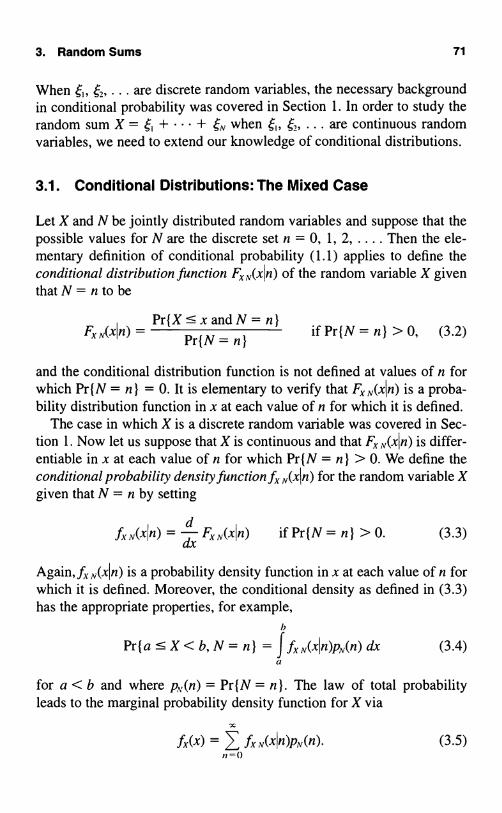
3. Random Sums 71
When 6 62, ... are discrete random variables, the necessary backgroundin conditional probability was covered in Section 1. In order to study therandom sum X = 6, + + 6n, when 6 ,, ... are continuous randomvariables, we need to extend our knowledge of conditional distributions.
3.1. Conditional Distributions: The Mixed Case
Let X and N be jointly distributed random variables and suppose that thepossible values for N are the discrete set n = 0, 1, 2, .... Then the ele-mentary definition of conditional probability (1.1) applies to define theconditional distribution function FxN(xIn) of the random variable X giventhat N = n to be
F (xIn) =F.Pr{X<xandN=n}
if Pr{N = n} > 0, (3.2)Pr{N=n}
and the conditional distribution function is not defined at values of n forwhich Pr{N = n} = 0. It is elementary to verify that Fx,v(xln) is a proba-bility distribution function in x at each value of n for which it is defined.
The case in which X is a discrete random variable was covered in Sec-tion 1. Now let us suppose that X is continuous and that FF,v(xln) is differ-entiable in x at each value of n for which Pr{N = n} > 0. We define theconditional probability density function fx N(xl n) for the random variable Xgiven that N = n by setting
ftN(xln) = d Fx (xln) if Pr(N = n) > 0. (3.3)
Again, fx,. (xI n) is a probability density function in x at each value of n forwhich it is defined. Moreover, the conditional density as defined in (3.3)has the appropriate properties, for example,
v
Pr{ a < X < b, N = n } =f (3.4)a
for a < b and where p\,(n) = Pr{N = n). The law of total probabilityleads to the marginal probability density function for X via
.fx(x) = Y, fx,v(xIn)pn,(n). (3.5)11=0

72 II Conditional Probability and Conditional Expectation
Suppose that g is a function for which E[Ig(X)I] < oo. The conditionalexpectation of g(X) given that N = n is defined by
E[g(X)IN = n] = J g(x)fXN(xln) dx. (3.6)
Stipulated thus, E[g(X)IN = n] satisfies the properties listed in (1.7) to(1.15) for the joint discrete case. For example, the law of total probability is
00
E[g(X)] = 7, E[g(X)IN= n]PN(n) = E{E[g(X)IN]}.n=o
3.2. The Moments of a Random Sum
Let us assume that k and N have the finite moments
(3.7)
E[lk] = I-L, Var[ek] = o,',
E[N] = v, Var[N] = 7-,(3.8)
and determine the mean and variance for X = 6, + + 6N as defined in(3.1). The derivation provides practice in manipulating conditional expec-tations, and the results,
E[X] = µv, Var[X] = vo + µ2T, (3.9)
are useful and important. The properties of conditional expectation listedin (1.7) to (1.15) justify the steps in the determination.
If we begin with the mean E[X], thenx
E[X] _ > E[XIN = n]pN(n) [(by (1.15)]n=0
x
E[, + +NIN = n]pN(n) (definition of X)n=1
E[e, + ... + e,JN = n]PN(n) [by (1.9)]n=1
x
6,,JpN(n) [by (1.10)]n=
x
lu 7, nPN(n) = µµv,t=1

3. Random Sums 73
To determine the variance, we begin with the elementary step
Var[X] = E[(X - µv)2] = E[(X - Nµ + Nµ - vµ)2]
= E[(X - Nµ)2] + E[µ2(N - v)2] (3.10)
+ 2E[p(X - Nµ)(N - v)].
Then xE[(X - Nµ)22] = Y E[(X - Nµ)2 IN = n]PN(n)
_ E[(6, +...+fn-nµ)2N=n]PN(n)n=1
and
n=1npN(n) = va-22,
E[A2(N - v)22] = µ2E[(N - v)2] = A2 T2,
whilex
E[p(X - Nµ)(N - v)] = µ7 E[(X - np)(n - v)IN = n]p,(n),1=0
- v)E[(X - nµ)I N = n] pN(n)
=0(because E[(X - nµ)IN = n] = nµ] = 0). Then (3.10)with the subsequent three calculations validates the variance of X as statedin (3.9).
Example The number of offspring of a given species is a random vari-able having probability mass function p(k) for k = 0, 1. .... A populationbegins with a single parent who produces a random number N of progeny,each of which independently produces offspring according to p(k) to forma second generation. Then the total number of descendants in the secondgeneration may be written X = 6, + + ,,,, where k is the number ofprogeny of the kth offspring of the original parent. Let E[N] = E[6k] = µand Var[N] = Var[ k] = 0,22. Then
E[X] = µ2 and Var[X] = µw2(1 + µ).
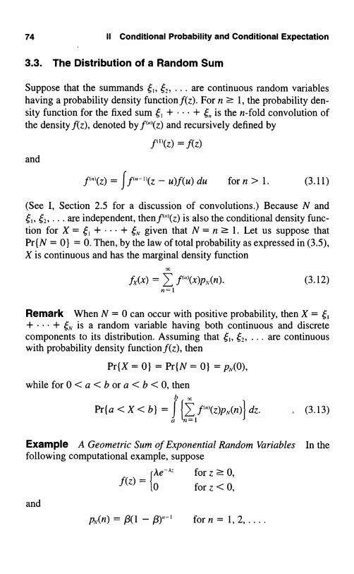
74 11 Conditional Probability and Conditional Expectation
3.3. The Distribution of a Random Sum
Suppose that the summands ,, 62, ... are continuous random variableshaving a probability density functionf(z). For n ? 1, the probability den-sity function for the fixed sum , + + is the n-fold convolution ofthe density f(z), denoted by fl'°(z) and recursively defined by
f f `(z) = f(z)and
f'"'(z) = f f"'-"(z - u)f(u) du for n > 1. (3.11)
(See I, Section 2.5 for a discussion of convolutions.) Because N and62.... are independent, then fl"'(z) is also the conditional density func-
tion for X = 6, + + 6, given that N = n ? 1. Let us suppose thatPr{N = 0} = 0. Then, by the law of total probability as expressed in (3.5),X is continuous and has the marginal density function
.ff(x) = , f O(x)pN(n)n
(3.12)
Remark When N = 0 can occur with positive probability, then X = ,+ + N is a random variable having both continuous and discretecomponents to its distribution. Assuming that 62, ... are continuouswith probability density function f(z), then
Pr{X=0} =Pr{N=0) =p,,,(0),
while for 0 < a < b or a < b < 0, thenG x
Pr(a < X < b} = f { f("'(z)pN(n)I dz. (3.13)n-i
Example A Geometric Sum of Exponential Random Variables In thefollowing computational example, suppose
Ae-A= for z ? 0,f (z) = {0 for z < 0,
and
pN(n) = /3(1 - f3)"-' for n = 1, 2, ... .

3. Random Sums 75
For n ? 1, the n-fold convolution of f(z) is the gamma density
111
f c"o(z) (n /--1)!z"-le-Az
0
for z ? 0,
forz<0.
(See I, Section 4.4 for discussion.)The density for X = , + + N is given, according to (3.5), by
W
fx(z) = fc")(z)PN(n)
n=1
All
= FA(1 -tie1 -Az\
= Azeau pr
= Age-ARz, z >_ 0.
Surprise! X has an exponential distribution with parameter A/3.
Example Stock Price Changes Stochastic models for price fluctua-tions of publicly traded assets were developed as early as 1900.
Let Z denote the difference in price of a single share of a certain stockbetween the close of one trading day and the close of the next. For anactively traded stock, a large number of transactions take place in a singleday, and the total daily price change is the sum of the changes over theseindividual transactions. If we assume that price changes over successivetransactions are independent random variables having a common finitevariance,' then the central limit theorem applies. The price change overa large number of transactions should follow a normal, or Gaussian,distribution.
' Rather strong economic arguments in support of these assumptions can be given. Theindependence follows from concepts of a "perfect market," and the common variance fromnotions of time stationarity.

76 II Conditional Probability and Conditional Expectation
A variety of empirical studies have supported this conclusion. For themost part, these studies involved price changes over a fixed number oftransactions. Other studies found discrepancies in that both very small andvery large price changes occurred more frequently in the data than sug-gested by normal theory. At the same time, intermediate-size pricechanges were underrepresented in the data. For the most part these stud-ies examined price changes over fixed durations containing a randomnumber of transactions.
A natural question arises: Does the random number of transactions in agiven day provide a possible explanation for the departures from normal-ity that are observed in data of daily price changes? Let us model the dailyprice change in the form
o+X, (3.14)
where to, t; ... are independent normally distributed random variableswith common mean zero and variance o r2, and N has a Poisson distribu-tion with mean v.
We interpret N as the number of transactions during the day, ; fori ? 1 as the price change during the ith transaction, and o as an initialprice change arising between the close of the market on one day and theopening of the market on the next. (An obvious generalization wouldallow the distribution of o to differ from that of t,, .Z..... )
Conditioned on N = n, the random variable Z = io + , + ... + isnormally distributed with mean zero and variance (n + 1)o . The condi-tional density function is
z
,(z) =2-Tr(n + 1)o-
exp{2 (n + 1)o-2J.
Since the probability mass function for N is
Xle-A
p,,,(n)= , n=0,1,...,.n!
using (3.12) we determine the probability density function for the dailyprice change to be
Alle-A
.fZ(z) (P.(z) n.
,1=o .

Exercises 77
The formula for the density ff(z) does not simplify. Nevertheless, numer-ical calculations are possible. When A = 1 and 0.2 = 1, then (3.9) showsthat the variance of the daily price change Z in the model (3.14) isVar[Z] _ (1 + A)o-2 = 1. Thus comparing the density ff(z) when A = 1and o.2 = ; to a normal density with mean zero and variance, one shedssome light on the question at hand.
The calculations were carried out and are shown in Figure 3.1.The departure from normality that is exhibited by the random sum in
Figure 3.1 is consistent with the departure from normality shown by stockprice changes over fixed time intervals. Of course, our calculations do notprove that the observed departure from normality is caused by the randomnumber of transactions in a fixed time interval. Rather, the calculationsshow only that such an explanation is consistent with the data and is,therefore, a possible cause.
2
Figure 3.1 A standard normal density (solid line) as compared to a density fora random sum (dashed line). Both densities have zero mean and unit variance.
Exercises
3.1. A six-sided die is rolled, and the number N on the uppermost face isrecorded. Then a fair coin is tossed N times, and the total number Z of headsto appear is observed. Determine the mean and variance of Z by viewing Zas a random sum of N Bernoulli random variables. Determine the proba-bility mass function of Z, and use it to find the mean and variance of Z.

78 11 Conditional Probability and Conditional Expectation
3.2. Six nickels are tossed, and the total number N of heads is observed.Then N dimes are tossed, and the total number Z of tails among the dimesis observed. Determine the mean and variance of Z. What is the probabil-ity that Z = 2?
3.3. Suppose that upon striking a plate a single electron is transformedinto a number N of electrons, where N is a random variable with mean p.and standard deviation o. Suppose that each of these electrons strikes asecond plate and releases further electrons, independently of each otherand each with the same probability distribution as N. Let Z be the totalnumber of electrons emitted from the second plate. Determine the meanand variance of Z.
3.4. A six-sided die is rolled, and the number N on the uppermost faceis recorded. From a jar containing 10 tags numbered 1 , 2, ... , 10 we thenselect N tags at random without replacement. Let X be the smallest num-ber on the drawn tags. Determine Pr (X = 2) and E[X].
3.5. The number of accidents occurring in a factory in a week is a Pois-son random variable with mean 2. The number of individuals injured indifferent accidents is independently distributed, each with mean 3 andvariance 4. Determine the mean and variance of the number of individu-als injured in a week.
Problems
3.1. The following experiment is performed: An observation is made ofa Poisson random variable N with parameter A. Then N independentBernoulli trials are performed, each with probability p of success. Let Zbe the total number of successes observed in the N trials.
(a) Formulate Z as a random sum and thereby determine its mean andvariance.
(b) What is the distribution of Z?
3.2. For each given p, let Z have a binomial distribution with parame-ters p and N. Suppose that N is itself binomially distributed with parame-ters q and M. Formulate Z as a random sum and show that Z has a bino-mial distribution with parameters pq and M.

4. Conditioning on a Continuous Random Variable 79
3.3. Suppose that f,, ,, ... are independent and identically distributedwith Pr(6R = ± 11 = ;. Let N be independent of 6, ,2, ... and follow thegeometric probability mass function
p,,(k) = all - a)' for k = 0, 1, ... ,where 0 < a < 1. Form the random sum Z = , + +
(a) Determine the mean and variance of Z.(b) Evaluate the higher moments m, = E[Z'] and m,, = E[Z°].
Hint: Express Z' in terms of the ;'s where C; = 1 and E[6; ;] = 0.
3.4. Suppose 6 62, ... are independent and identically distributed ran-dom variables having mean µ and variance 0-2 . Form the random sumSN=6i +...+6N
(a) Derive the mean and variance of S, when N has a Poisson distrib-ution with parameter A.
(b) Determine the mean and variance of S, when N has a geometric dis-tribution with mean A = (1 - p)lp.
(c) Compare the behaviors in (a) and (b) as A - .
3.5. To form a slightly different random sum, let &, ,, . . . be indepen-dent identically distributed random variables and let N be a nonnegativeinteger-valued random variable, independent of , .... The first twomoments are
E[6,] = µ, Var[ R] _ 0-2,
E[N] = v, Var[N] = T'-,
Determine the mean and variance of the random sum Z =o + +
4. Conditioning on a Continuous Random Variable2
Let X and Y be jointly distributed continuous random variables with jointprobability density function ff.,.(x, y). We define the conditional probabil-ity density function fx,,(xl y) for the random variable X given that Y = y bythe formula
2 The reader may wish to defer reading this section until encountering VII, on renewalprocesses, where conditioning on a continuous random variable first appears.
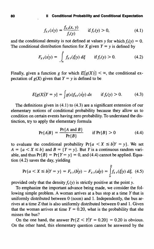
80 11 Conditional Probability and Conditional Expectation
fxr(xI y) = f fr(y)) if ff (y) > 0, (4.1)
and the conditional density is not defined at values y for which fy(y) = 0.The conditional distribution function for X given Y = y is defined by
Fx r(xjy) = f fx r(61y) d if fr(y) > 0. (4.2)-z
Finally, given a function g for which E[I g(X )I ] < oo, the conditional ex-pectation of g(X) given that Y = y is defined to be
E[g(X)I Y = yl = Jg(x)fxy(xy) dx if fr(y) > 0. (4.3)
The definitions given in (4.1) to (4.3) are a significant extension of ourelementary notions of conditional probability because they allow us tocondition on certain events having zero probability. To understand the dis-tinction, try to apply the elementary formula
Pr{AIB} =Pr{A and B}
if Pr{B} > 0 (4.4)Pr{B}
to evaluate the conditional probability Pr{a < X <_ bIY = y}. We setA = (a < X:5 b) and B = {Y = y}. But Y is a continuous random vari-able, and thus Pr{B} = Pr( Y = y) = 0, and (4.4) cannot be applied. Equa-tion (4.2) saves the day, yielding
b
Pr{a < X : bIY = y) = Fx r(bly) - Fx r( I y) (4.5)a
provided only that the density fr(y) is strictly positive at the pointy.To emphasize the important advance being made, we consider the fol-
lowing simple problem. A woman arrives at a bus stop at a time Y that isuniformly distributed between 0 (noon) and 1. Independently, the bus ar-rives at a time Z that is also uniformly distributed between 0 and 1. Giventhat the woman arrives at time Y = 0.20, what is the probability that shemisses the bus?
On the one hand, the answer Pr(Z < YIY = 0.20) = 0.20 is obvious.On the other hand, this elementary question cannot be answered by the

4. Conditioning on a Continuous Random Variable 81
elementary conditional probability formula (4.4) because the event(Y = 0.20) has zero probability. To apply (4.1), start with the joint den-sity function
r1AY(z' y) = 0 elsewhere,
and change variables according to X = Y - Z. Then
fx.r(x,y)= 1 for05y<l,y- 1 :! x:y,and, applying (4.1), we find that
fx,r(x, 0.20)fx r(xI0.20) =
fr(0.20)= 1 for -0.80 <- x :5 0.20.
Finally,00
Pr(Z<YIY=0.20) =Pr(X>OIY=0.20) = Jfx (x0.20) dx = 0.20.0
We see that the definition in (4.1) leads to the intuitively correct answer.The conditional density function that is prescribed by (4.1) possesses
all of the properties that are called for by our intuition and the basic con-cept of conditional probability. In particular, one can calculate the proba-bility of joint events by the formula
d b
Pr{a < X < b, c < Y < d} = J(Jfx y(xly) dx}fy(y) dy, (4.6)c a
which becomes the law of total probability by setting c = -oo andd=+oo:
+00 b
Pr(a < X < b} = f {Jf(xy) dx}fy(y) dy. (4.7)x a
For the same reasons, the conditional expectation as defined in (4.3) sat-isfies the requirements listed in (1.7) to (1.11). The property (1.12),adapted to a continuous random variable Y, is written
E[g(X)h(Y)] = E{h(Y)E[g(X)IY])
= Jh(y)E[g(X)Y = y]ff(y) dy, (4.8)

82 II Conditional Probability and Conditional Expectation
valid for any bounded function h, and assuming E[Ig(X)I] < x. Whenh(y) = 1, we recover the law of total probability in the form
E[g(X)] = E{E[g(X)I Yl }= JE[g(X)Y = y].fr(y) dy. (4.9)
Both the discrete and continuous cases of (4.8) and (4.9) are containedin the expressions
E[g(X)h(Y)] = E{h(Y)E[g(X)IY]}= Jh(y)E[g(X)Y= y] dFF(y), (4.10)
dnd
E[g(X)] = E{E[g(X)IY]}= JE[g(X)Y = y] dFF(y). (4.11)
[See the discussion following (2.9) in I for an explanation of the symbol-ism in (4.10) and (4.11).]
The following exercises provide practice in deriving conditional prob-ability density functions and in manipulating the law of total probability.
Example Suppose X and Y are jointly distributed random variableshaving the density function
.fxr(x, y) = 1e for x, y > 0.y
We first determine the marginal density for y, obtainingx
.fr(y) = Jfxy(X, y) dx0
X
= e-, f Y dx = e
Then0
for t'>0.
fx r(xl y) = f.f(c')) = y- 'e-for x, y > 0.
That is, conditional on Y = y, the random variable X has an exponentialdistribution with parameter 1/y. It is easily seen that E[XI Y = y] = Y.
Example For each given p, let X have a binomial distribution with pa-rameters p and N. Suppose that p is uniformly distributed on the interval[0, 1]. What is the resulting distribution of X?
We are given the marginal distribution for p and the conditional distri-

4. Conditioning on a Continuous Random Variable 83
bution for X. Applying the law of total probability and the beta integral I,(6.16) we obtain
Pr{X = k} = JPr{X = klp = }f,(O de0
_ N!_ kl- Nkd0 k!(N - k)!
N! k!(N - k)!k!(N - k)! (N + 1)!
1
N+1 fork= 0, 1,...,N.
That is, X is uniformly distributed on the integers 0, 1, . . . , N.When p has the beta distribution with parameters r and s, then similar
calculations give
I
Pr{X = k} =k!(N - k)!
Y)r(S f f.-.(1 - - 6)"-k d
_ (N) I'(r + s)r(r + k)I'(s + N - k)- kI'(r)I'(s)I'(N + r + s)
fork=0, 1,...,N.
Example A random variable Y follows the exponential distributionwith parameter 0. Given that Y = y, the random variable X has a Poissondistribution with mean y. Applying the law of total probability then yields
x
Pr{X = k} = yKe-Joedy0
6 f yke-(,+0)`' dyk! o
xe
uke " duk!(1+ O)k+1 0
0
0
(1 + O)k+Ifor k= 0, 1, ... .

84 II Conditional Probability and Conditional Expectation
Suppose that Y has the gamma density
fr(Y) = r(a)(ey)a-ie-m, y ? 0.
Then similar calculations yield
yke-' B(OY
p,,Pr{X = k} = f k I'0
)a-Ie-° dy
0
Ba f uk+a- I e-" duk!1'(a)(1 + 9)k+a
0
k!F(a) )
0
k( l+0)1+0)
This is the negative binomial distribution.
Exercises
k = 0,1,....
4.1. Suppose that three contestants on a quiz show are each given thesame question, and that each answers it correctly, independently of theothers, with probability p. But the difficulty of the question is itself a ran-dom variable, so let us suppose, for the sake of illustration, that p is uni-formly distributed over the interval (0, 1]. What is the probability that ex-actly two of the contestants answer the question correctly?
4.2. Suppose that three components in a certain system each functionwith probability p and fail with probability 1 - p, each component oper-ating or failing independently of the others. But the system is in a randomenvironment, so that p is itself a random variable. Suppose that p is uni-formly distributed over the interval (0, 1]. The system operates if at leasttwo of the components operate. What is the probability that the systemoperates?
4.3. A random variable T is selected that is uniformly distributed overthe interval (0, 1]. Then a second random variable U is chosen, uniformlydistributed on the interval (0, T]. What is the probability that U exceeds 1?

Problems 85
4.4. Suppose X and Y are independent random variables, each exponen-tially distributed with parameter A. Determine the probability densityfunction for Z = X/Y.
4.5. Let U be uniformly distributed over the interval [0, L] where L fol-lows the gamma density fL(x) = xe for x >_ 0. What is the joint densityfunction of U and V = L - U?
Problems
4.1. Suppose that the outcome X of a certain chance mechanism de-pends on a parameter p according to Pr{X = 1) = p and Pr{X = 0} =1 - p, where 0 < p < 1. Suppose that p is chosen at random, uniformlydistributed over the unit interval [0, 1], and then that two independent out-comes X, and X, are observed. What is the unconditional correlation co-efficient between X, and X,?
Note: Conditionally independent random variables may become de-pendent if they share a common parameter.
4.2. Let N have a Poisson distribution with parameter A > 0. Supposethat, conditioned on N = n, the random variable X is binomially distrib-uted with parameters N = n and p. Set Y = N - X. Show that X and Yhave Poisson distributions with respective parameters Ap and A(1 - p)and that X and Y are independent.
Note: Conditionally dependent random variables may become inde-pendent through randomization.
4.3. Let X have a Poisson distribution with parameter A > 0. Suppose Aitself is random, following an exponential density with parameter 0.
(a) What is the marginal distribution of X?(b) Determine the conditional density for A given X = k.
4.4. Suppose X and Y are independent random variables having thesame Poisson distribution with parameter A, but where A is also random,being exponentially distributed with parameter 0. What is the conditionaldistribution for X given that X + Y = n?

86 II Conditional Probability and Conditional Expectation
4.5. Let X and Y be jointly distributed random variables whose jointprobability mass function is given in the following table:
x
-1 0 1
1
9
2
9 0
y 9
2
9
1 9 0 19
p(x,y)=Pr{x=x,Y=y}
Show that the covariance between X and Y is zero even though X and Yare not independent.
4.6. Let Xo, x, X2, . . . be independent identically distributed nonnega-tive random variables having a continuous distribution. Let N be the firstindex k for which Xk > Xo. That is, N = 1 if X, > Xo, N = 2 if X, X0 andX2 > X0, etc. Determine the probability mass function for N and the meanE[N]. (Interpretation: X0, X,.... are successive offers or bids on a car thatyou are trying to sell. Then N is the index of the first bid that is better thanthe initial bid.)
4.7. Suppose that X and Y are independent random variables, each hav-ing the same exponential distribution with parameter a. What is the con-ditional probability density function for X, give that Z = X + Y: = z?
4.8. Let X and Y have the joint normal density given in I, (4.16). Showthat the conditional density function for X, given that Y = y, is normalwith moments
AXr=!'fi'x+PoxPY (y - A v)
and
axr=cTxV1-Pl.

5. Martingales 87
5. Martingales*
Stochastic processes are characterized by the dependence relationshipsthat exist among their variables. The martingale property is one such re-lationship that captures a notion of a game being fair. The martingaleproperty is a restriction solely on the conditional means of some of thevariables, given values of others, and does not otherwise depend on theactual distribution of the random variables in the stochastic process. De-spite the apparent weakness of the martingale assumption, the conse-quences are striking, as we hope to suggest.
5.1. The Definition
We begin the presentation with the simplest definition.
Definition A stochastic process {X,,; n = 0, 1.... } is a martingale if forn=0,1,...,
(a) E[IX Il < 00,
and
(b) XTaking expectations on both sides of (b),
Xo, . . . , E{X,,},
and using the law of total probability in the form
X ... ,
shows that
and consequently, a martingale has constant mean:
E[X0] = E[XA] = 0 : k <_ n. (5.1)
* Some problems scattered throughout the text call for the student to identify certain sto-chastic processes as martingales. Otherwise, the material of this section is not used in thesequel.
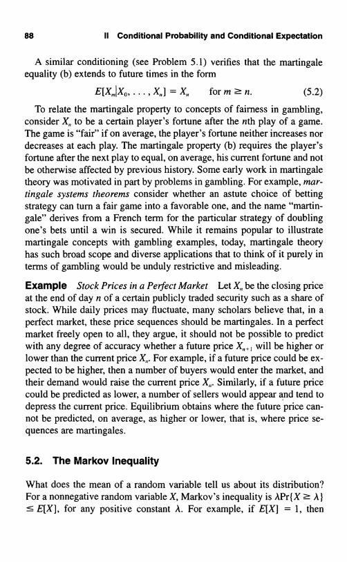
88 II Conditional Probability and Conditional Expectation
A similar conditioning (see Problem 5.1) verifies that the martingaleequality (b) extends to future times in the form
E[X,,,IXO, . . . , X,, for m ? n. (5.2)
To relate the martingale property to concepts of fairness in gambling,consider X to be a certain player's fortune after the nth play of a game.The game is "fair" if on average, the player's fortune neither increases nordecreases at each play. The martingale property (b) requires the player'sfortune after the next play to equal, on average, his current fortune and notbe otherwise affected by previous history. Some early work in martingaletheory was motivated in part by problems in gambling. For example, mar-tingale systems theorems consider whether an astute choice of bettingstrategy can turn a fair game into a favorable one, and the name "martin-gale" derives from a French term for the particular strategy of doublingone's bets until a win is secured. While it remains popular to illustratemartingale concepts with gambling examples, today, martingale theoryhas such broad scope and diverse applications that to think of it purely interms of gambling would be unduly restrictive and misleading.
Example Stock Prices in a Perfect Market Let X,, be the closing priceat the end of day n of a certain publicly traded security such as a share ofstock. While daily prices may fluctuate, many scholars believe that, in aperfect market, these price sequences should be martingales. In a perfectmarket freely open to all, they argue, it should not be possible to predictwith any degree of accuracy whether a future price will be higher orlower than the current price X,,. For example, if a future price could be ex-pected to be higher, then a number of buyers would enter the market, andtheir demand would raise the current price X,,. Similarly, if a future pricecould be predicted as lower, a number of sellers would appear and tend todepress the current price. Equilibrium obtains where the future price can-not be predicted, on average, as higher or lower, that is, where price se-quences are martingales.
5.2. The Markov Inequality
What does the mean of a random variable tell us about its distribution?For a nonnegative random variable X, Markov's inequality is APr{X ? A)s E[X], for any positive constant A. For example, if E[X] = 1, then

S. Martingales 89
Pr(X ? 4} <_ , no matter what the actual distribution of X is. The proofuses two properties: (i) X > 0 (X is a nonnegative random variable); and(ii) E[X1{X ? A}] ? APr{X ? A}. (Recall that 1(A) is the indicator of anevent A and is one if A occurs and zero otherwise. See I, Section 3.1.)Then by the law of total probability,
E[X] = E[X1{X ? A}] + E[X1{X < A)]
E[X1{X ? All (by (i))
APr{X ? A), (by (ii))
and Markov's inequality results.
5.3. The Maximal Inequality for Nonnegative Martingales
Because a martingale has constant mean, Markov's inequality applied toa nonnegative martingale immediately yields
A) <_ E[X0],A>0.
We will extend the reasoning behind Markov's inequality to achieve an in-equality of far greater power:
X ? A} E[X °] . (5.3)
Instead of limiting the probability of a large value for a single observationX,,, the maximal inequality (5.3) limits the probability of observing a largevalue anywhere in the time interval 0, . . . , m, and since the right side of(5.3) does not depend on the length of the interval, the maximal inequal-ity limits the probability of observing a large value at any time in the in-finite future of the martingale!
In order to prove the maximal inequality for nonnegative martingales,we need but a single additional fact: If X and Y are jointly distributed ran-dom variables and B is an arbitrary set, then
E[X1{Yin B}] = E[E{XIY}1{Yin B}]. (5.4)
But (5.4) follows from the conditional expectation property (1.12),E[g(X)h(Y)] = E{h(Y)E[g(X)IY]}, with g(x) = x and h(y) = 1(y in B).
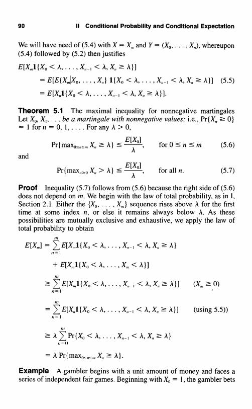
90 II Conditional Probability and Conditional Expectation
We will have need of (5.4) with X = X,,, and Y = (X0, ... , X, ), whereupon(5.4) followed by (5.2) then justifies
E[X,,1{X0<A,...,X,,.
=E[E{X,,IX0,...,X,,}1{X0<
A, <A,X,,_A}].
Theorem 5.1 The maximal inequality for nonnegative martingalesLet X0, X ... be a martingale with nonnegative values; i.e., Pr(X ? 0)= 1 for n = 0, 1. .... For any A > 0,
E[X0]Pr X ? A) s
and
for (5 6).
A
Pr{ X > A) E[X °] , for all n. (5.7)
Proof Inequality (5.7) follows from (5.6) because the right side of (5.6)does not depend on m. We begin with the law of total probability, as in I,Section 2.1. Either the {X0, ... , X,,, } sequence rises above A for the firsttime at some index n, or else it remains always below A. As thesepossibilities are mutually exclusive and exhaustive, we apply the law oftotal probability to obtain
,,,
E[X ,] = >, E[X,,,1 {X < A,... , A, X,, ? A}!t=
m
M
,X,,,<A}]
0)11 =
E[X,,1(X0 < A__, A, X,, ? A)] (using 5.5))
A>,Pr{X0 < A_ X,,-, < A, X,, Al,1=o
= A Pr f X,, ? A).
Example A gambler begins with a unit amount of money and faces aseries of independent fair games. Beginning with X = 1, the gambler bets

S. Martingales 91
the amount p, 0 < p < 1. If the first game is a win, which occurs withprobability Z, the gambler's fortune is X, = 1 + pXo = 1 + p. If the firstgame is a loss, then X, = 1 - pXo = 1 - p. After the nth play and with acurrent fortune of X,,, the gambler wagers pX,,, and
((1 + p)X,, with probability Z,
1(1 - p)X with probability Z.
Then is a nonnegative martingale, and the maximal inequality (5.6)with A = 2, for example, asserts that the probability that the gambler everdoubles his money is less than or equal to z, and this holds no matter whatthe game is, as long as it is fair, and no matter what fraction p of his for-tune is wagered at each play. Indeed, the fraction wagered may vary fromplay to play, as long as it is chosen without knowledge of the nextoutcome.
As amply demonstrated by this example, the maximal inequality is avery strong statement. Indeed, more elaborate arguments based on themaximal and other related martingale inequalities are used to show that anonnegative martingale converges: If is a nonnegative martingale,then there exists a random variable, let us call it X., for which lim,,. X,, =X.. We cannot guarantee the equality of the expectations in the limit, butthe inequality E[X0] ? E[X] ? 0 can be established.
Example In III, Section 8, we will introduce the branching processmodel for population growth. In this model, X,, is the number of individu-als in the population in the nth generation, and µ > 0 is the mean familysize, or expected number of offspring of any single individual. The meanpopulation size in the nth generation is Xoµ". In this branching processmodel, X,,/µ" is a nonnegative martingale (see III, Problem 8.4), and themaximal inequality implies that the probability of the actual populationever exceeding ten times the mean size is less than or equal to 1/10. Thenonnegative martingale convergence theorem asserts that the evolution ofsuch a population after many generations may be described by a singlerandom variable X. in the form
X -== X,,µ", for large n.
Example How NOT to generate a uniformly distributed random vari-able An urn initially contains one red and one green ball. A ball is drawnat random and it is returned to the urn, together with another ball of the
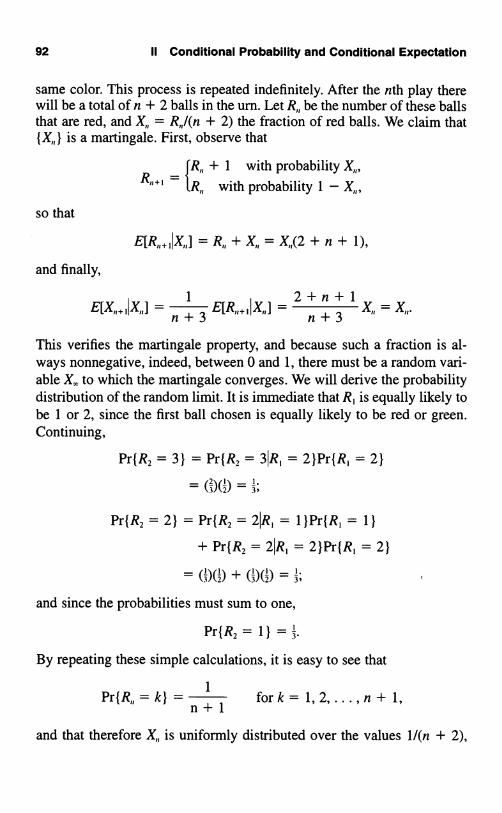
92 11 Conditional Probability and Conditional Expectation
same color. This process is repeated indefinitely. After the nth play therewill be a total of n + 2 balls in the urn. Let R,, be the number of these ballsthat are red, and X,, = 2) the fraction of red balls. We claim that
is a martingale. First, observe that
(R + 1 with probability X,,,
R with probability 1 - X,,,
so that
R,, + X,, = n + 1),
and finally,
E[X,,,,I X,,] = n + 3E[R,,+,IX,,] =
2
n + 3 1 X" = X.
This verifies the martingale property, and because such a fraction is al-ways nonnegative, indeed, between 0 and 1, there must be a random vari-able X. to which the martingale converges. We will derive the probabilitydistribution of the random limit. It is immediate that R, is equally likely tobe 1 or 2, since the first ball chosen is equally likely to be red or green.Continuing,
Pr{R2 = 3) _ //Pr//{R, = 31R, = 2}Pr{R1 = 21
l3)(2) 3,
Pr{R, = 2} = Pr{R2 = 2IR, = 1 }Pr{R, = 1)
(+ Pr{R2//=((21R, = 2}Pr{R1 = 21
(3)(/(2) + (3)\2) = 3+
and since the probabilities must sum to one,
Pr{R, = 1) = .
By repeating these simple calculations, it is easy to see that
1
n+1 fork=1,2,...,n+1,
and that therefore X,, is uniformly distributed over the values 1/(n + 2),

Exercises 93
2/(n + 2), . . . , (n + 1)/(n + 2). This uniform distribution must prevail inthe limit, which leads to
Pr{X,,-x} =x for0<x<1.Think about this remarkable result for a minute! If you sit down in frontof such an urn and play this game, eventually the fraction of red balls inyour urn will stabilize in the near vicinity of some value, call it U. If I playthe game, the fraction of red balls in my urn will stabilize also, but at an-other value, U'. Anyone who plays the game will find the fraction of redballs in the urn tending towards some limit, but everyone will experiencea different limit. In fact, each play of the game generates a fresh, uni-formly distributed random variable, in the limit. Of course, there maybe faster and simpler ways to generate uniformly distributed randomvariables.
Martingale implications include many more inequalities and conver-gence theorems. As briefly mentioned at the start, there are so-called sys-tems theorems that delimit the conditions under which a gambling system,such as doubling the bets until a win is secured, can turn a fair game intoa winning game. A deeper discussion of martingale theory would take uswell beyond the scope of this introductory text, and our aim must be lim-ited to building an enthusiasm for further study. Nevertheless, a large va-riety of important martingales will be introduced in the Problems at theend of each section in the remainder of the book.
Exercises
5.1. Let X be an exponentially distributed random variable with meanE[X] = 1. For x = 0.5, 1, and 2, compare Pr{X > x} with the Markov in-equality bound E[X]/x.
5.2. Let X be a Bernoulli random variable with parameter p. ComparePr{X ? 1) with the Markov inequality bound.
5.3. Let 6 be a random variable with mean µ and standard deviation a-.Let X = (6 - µ)Z. Apply Markov's inequality to X to deduce Chebyshev'sinequality:
Pr { - µl ? e } s 0Zfor any e > 0.
8

94 II Conditional Probability and Conditional Expectation
Problems
5.1. Use the law of total probability for conditional expectationsE[E{XIY, Z}IZ] = E[XIZ] to show
E[E{X,,+2IXO, ... , I Xo, ... ,X is a martingale.
XO, ... , X.
5.2. Let U,, U2, . . . be independent random variables each uniformlydistributed over the interval (0, 1]. Show that X0 = 1 and X,, = 2"U, Ufor n = 1, 2.... defines a martingale.
5.3 Let So = 0, and for n ? 1, let S,, = s, + + s be the sum of nindependent random variables, each exponentially distributed with meanE[e] = 1. Show that
defines a martingale.
5.4. Let 62, ... be independent Bernoulli random variables withparameter p, 0 < p < 1. Show that X. = 1 and X,, = p" 6, ... ,,, n = 1,
2, . . . , defines a nonnegative martingale. What is the limit of X,, as n-oo?
5.5. Consider a stochastic process that evolves according to the follow-ing laws: If X,, = 0, then X,,+, = 0, whereas if X,, > 0, then
IX,, + 1 with probability 2X",
X - 1 with probability Z .
(a) Show that X,, is a nonnegative martingale.(b) Suppose that X0 = i > 0. Use the maximal inequality to bound
Pr{X ? N for some n ? OIXO = i}.
Note: X,, represents the fortune of a player of a fair game who wagers $1at each bet and who is forced to quit if all money is lost (X,, = 0). Thisgambler's ruin problem is discussed fully in III, Section 5.3.

Chapter IIIMarkov Chains: Introduction
1. Definitions
A Markov process {X,} is a stochastic process with the property that, giventhe value of X the values of X, for s > t are not influenced by the valuesof X for u < t. In words, the probability of any particular future behaviorof the process, when its current state is known exactly, is not altered byadditional knowledge concerning its past behavior. A discrete-timeMarkov chain is a Markov process whose state space is a finite or count-able set, and whose (time) index set is T = (0, 1, 2, ...). In formal terms,the Markov property is that
Pr{X,,+ = jIXO = i0, ... , X = i}
(1.1)
for all time points n and all states i0 . , i, j.It is frequently convenient to label the state space of the Markov chain
by the nonnegative integers {0, 1, 2, ...}, which we will do unless thecontrary is explicitly stated, and it is customary to speak of X,, as being instate i if X,, = i.
The probability of X,,+, being in state j given that X,, is in state i is calledthe one-step transition probability and is denoted by P;"+'. That is,
P;;"+' = Pr{ jIX,, = i}. (1.2)

96 III Markov Chains: Introduction
The notation emphasizes that in general the transition probabilities arefunctions not only of the initial and final states, but also of the time oftransition as well. When the one-step transition probabilities are indepen-dent of the time variable n, we say that the Markov chain has stationarytransition probabilities. Since the vast majority of Markov chains that weshall encounter have stationary transition probabilities, we limit our dis-cussion to this case. Then P ,j',"" = Pij is independent of n, and Pij is theconditional probability that the state value undergoes a transition fromi to j in one trial. It is customary to arrange these numbers Pij in a matrix,i'n the infinite square array
PO0 Poi P02 P03
P10 Pn P12 P13
P20 P,, P22 P23
P=
PO P,,, P, P,
and refer to P = (IP;jJJ as the Markov matrix or transition probability ma-trix of the process.
The ith row of P, for i = 0, 1, . . . , is the probability distribution of thevalues of under the condition that X,, = i. If the number of states isfinite, then P is a finite square matrix whose order (the number of rows)is equal to the number of states. Clearly, the quantities Pij satisfy theconditions
P, ?0 fori,j=0,1,2,..., (1.3)
= 1 for i = 0, 1, 2, .... (1.4)j=0
The condition (1.4) merely expresses the fact that some transition occursat each trial. (For convenience, one says that a transition has occurredeven if the state remains unchanged.)
A Markov process is completely defined once its transition probabilitymatrix and initial state X0 (or, more generally, the probability distributionof X0) are specified. We shall now prove this fact.

1. Definitions 97
Let Pr{Xo = i} = pi. It is enough to show how to compute the quantities
Pr{Xo = i0, X, = i X2 = i,, ... , X = (1.5)
since any probability involving X;., ... , Xj,, for j, < ... < jR, can be ob-tained, according to the axiom of total probability, by summing terms ofthe form (1.5).
By the definition of conditional probabilities we obtain
Pr{Xo = i0, X, = i,, X, = i,..... X = i,r}
(1.6)
X Pr{X = i0, X, = i,, . . . , I.
Now, by the definition of a Markov process,
Pr{X,, = i I XO = i0, X, = i . . . ,
(1.7)= Pr{X,r = i,r1 X,_ = i,r_, } = Pi,r-
Substituting (1.7) into (1.6) gives
Pr{XO=io, X,=i......
Pr{X0 = i0, X, = i,, . .
Then, upon repeating the argument n - 1 additional times, (1.5) becomes
Pr{Xo = io, X, = i...... X,, =(1.8)
= pi Po.i, ... pill-
This shows that all finite-dimensional probabilities are specified once thetransition probabilities and initial distribution are given, and in this sensethe process is defined by these quantities.
Related computations show that (1.1) is equivalent to the Markov prop-erty in the form
Pr{X,,, = ji, . . . , io, ... , X" = ill)(1.9)
= j,, . . . , i X" ill)
for all time points n, m and all states io, . . . , i,,, 1, , j,,,. In other words,once (1.9) is established for the value m = 1, it holds for all m ? 1 aswell.
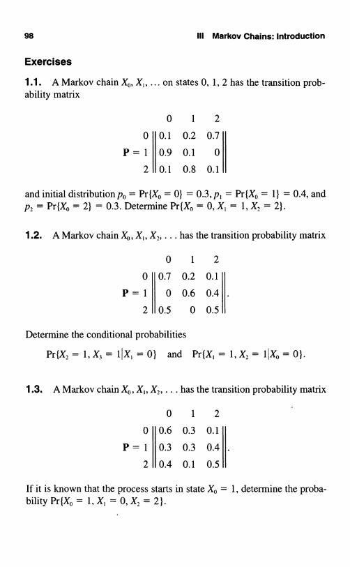
98 III Markov Chains: Introduction
Exercises
1.1. A Markov chain X,,, X ... on states 0, 1, 2 has the transition prob-ability matrix
0 1 2
0 0.1 0.2 0.7
P=1 0.9 0.1 0
2 0.1 0.8 0.1
and initial distribution p = Pr{Xo = 0) = 0.3, p, = Pr{Xp = 1) = 0.4, andp, = Pr{X = 2) = 0.3. Determine Pr{X = 0, X, = 1, X, = 2).
1.2. A Markov chain X, X, X,, . . . has the transition probability matrix
0 1 2
0 0.7 0.2 0.1
P=1 0 0.6 0.4
2 0.5 0 0.5
Determine the conditional probabilities
Pr{X, = 1, )(, = 1IX, = 0) and Pr{X1 = 1, X, = 1IX = 01.
1.3. A Markov chain X,,, X,, X2.... has the transition probability matrix
0 1 2
0 0.6 0.3 0.1
P=1 0.3 0.3 0.4
2 0.4 0.1 0.5
If it is known that the process starts in state X = 1, determine the proba-bility Pr{X = 1, X, = 0, X, = 2}.

Problems 99
1.4. A Markov chain X0, X,, X2, . . . has the transition probability matrix
0 1 2
0 0.1 0.1 0.8
P=1 0.2 0.2 0.6
2 0.3 0.3 0.4
Determine the conditional probabilities
Pr{X, = 1,X2= 1IX0 =0} and Pr{X2= 1,X3= IJX, =0}.
1.5. A Markov chain Xo, X,, X2, . . . has the transition probability matrix
0 1 2
0 0.3 0.2 0.5
P=1 0.5 0.1 0.4
2 0.5 0.2 0.3
and initial distribution po = 0.5 and p, = 0.5. Determine the probabilities
Pr(X0 = 1, X, = 1, X2 = 0} and Pr{X1 = 1, X2 = 1, X3 = 0}.
Problems
1.1. A simplified model for the spread of a disease goes this way: Thetotal population size is N = 5, of which some are diseased and the re-mainder are healthy. During any single period of time, two people are se-lected at random from the population and assumed to interact. The selec-tion is such that an encounter between any pair of individuals in thepopulation is just as likely as between any other pair. If one of these per-sons is diseased and the other not, then with probability a = 0.1 the dis-ease is transmitted to the healthy person. Otherwise, no disease transmis-sion takes place. Let X,, denote the number of diseased persons in thepopulation at the end of the nth period. Specify the transition probabilitymatrix.

100 III Markov Chains: Introduction
1.2. Consider the problem of sending a binary message, 0 or 1, througha signal channel consisting of several stages, where transmission througheach stage is subject to a fixed probability of error a. Suppose that X0 = 0is the signal that is sent and let X,, be the signal that is received at the nthstage. Assume that is a Markov chain with transition probabilitiesPoo a andP0,=P10=a,where 0<a<1.
(a) Determine Pr{Xo = 0, X, = 0, X, = 0}, the probability that no erroroccurs up to stage n = 2.
(b) Determine the probability that a correct signal is received at stage2.
Hint: This is Pr{Xo=O,X,=0,X,=0}+Pr{Xo=0,X,=1,X,=0}.
1.3. Consider a sequence of items from a production process, with eachitem being graded as good or defective. Suppose that a good item is fol-lowed by another good item with probability a and is followed by a de-fective item with probability 1 - a. Similarly, a defective item is followedby another defective item with probability /3 and is followed by a gooditem with probability 1 - /3. If the first item is good, what is the proba-bility that the first defective item to appear is the fifth item?
1.4. The random variables ,, 6z, ... are independent and with the com-mon probability mass function
k 0 1 2 3
Pr{6 = k} = 0.1 0.3 0.2 0.4
Set X0 = 0, and let X,, = max be the largest observed to date.Determine the transition probability matrix for the Markov chain {X,,}.
2. Transition Probability Matrices of a Markov Chain
A Markov chain is completely defined by its one-step transition probabil-ity matrix and the specification of a probability distribution on the state ofthe process at time 0. The analysis of a Markov chain concerns mainly thecalculation of the probabilities of the possible realizations of the process.

2. Transition Probability Matrices of a Markov Chain 101
Central in these calculations are the n-step transition probability matricesP'"' = IIP°;'M1. Here P;] denotes the probability that the process goes fromstate i to state j in n transitions. Formally,
P' = Pr(X,,,+,, = i). (2.1)
Observe that we are dealing only with temporally homogeneous processeshaving stationary transition probabilities, since otherwise the left side of(2.1) would also depend on m.
The Markov property allows us to express (2.1) in terms of JJP I asstated in the following theorem.
Theorem 2.1 The n-step transition probabilities of a Markov chainsatisfy
P;; PA P1; ,
k=0(2.2)
where we define
1
P;°' = {0ifi=j,ifi0j.
From the theory of matrices we recognize the relation (2.2) as the for-mula for matrix multiplication, so that P'"' = P x P("-''. By iterating thisformula, we obtain
P'"'=PXPX... XP=P"; (2.3)
n factors
in other words, the n-step transition probabilities P,] are the entries in thematrix P", the nth power of P.
Proof The proof proceeds via a first step analysis, a breaking down, oranalysis, of the possible transitions on the first step, followed by an appli-cation of the Markov property. The event of going from state i to state j inn transitions can be realized in the mutually exclusive ways of going tosome intermediate state k (k = 0, 1, ...) in the first transition, and thengoing from state k to state j in the remaining (n - 1) transitions. Becauseof the Markov property, the probability of the second transition is P(;-"and that of the first is clearly P, . If we use the law of total probability, then(2.2) follows. The steps are

102 III Markov Chains: IntroductionM
P;;)=Pr{X,, =jjXo=i} =7 Pr{X =j, X. =kjXo=i}
x
Xk=0
k=0
Pr{X1 = kiX0 = i} Pr(X = jjX0 = i, X, = k)
k=0P k Pkj(n-1)
If the probability of the process initially being in state j is pj, i.e., thedistribution law of X0 is Pr{Xo = j} = pj, then the probability of theprocess being in state k at time n is
Exercises
pR.° = p-P;'k = Pr{X = k}. (2.4)j=0
2.1. A Markov chain (X,,) on the states 0, 1, 2 has the transition proba-bility matrix
0 1 2
0.1 0.2 0.7
0.2 0.2 0.6
0.6 0.1 0.3
(a) Compute the two-step transition matrix P2.(b) What is Pr {)(, = 1I X, = 0}?(c) What is Pr{X3 = 1 Xo = 0)?
2.2. A particle moves among the states 0, 1, 2 according to a Markovprocess whose transition probability matrix is
0 1 2
0 0 2 z
1P=12 0 2
12 2 2 0
Let X,, denote the position of the particle at the nth move. CalculatePr(X,, =OJXo= 0)forn=0, 1,2,3,4.

Exercises 103
2.3. A Markov chain X0, X,, X,.... has the transition probability matrix
0 1 2
0 0.7 0.2 0.1
P=1 0 0.6 0.4
2 0.5 0 0.5
Determine the conditional probabilities
Pr{X1 = 1IXo=01 and Pr{X4 = 1jXo=01.
2.4. A Markov chain X0, X, X2.... has the transition probability matrix
0 1 2
0 0.6 0.3 0.1
P=1 0.3 0.3 0.4
2 0.4 0.1 0.5
If it is known that the process starts in state X0 = 1, determine the proba-bility Pr(X, = 2).
2.5. A Markov chain X0, X,, X,, . . . has the transition probability matrix
0 1 2
0 0.1 0.1 0.8
P=1 0.2 0.2 0.6
2 0.3 0.3 0.4
Determine the conditional probabilities
Pr{(3 = 1JX, = 0) and 1X0 = 0).
2.6. A Markov chain X0, X,, X,.... has the transition probability matrix
0 1 2
0 0.3 0.2 0.5
P=1 0.5 0.1 0.4
2 0.5 0.2 0.3

104 III Markov Chains: Introduction
and initial distribution po = 0.5 and p, = 0.5. Determine the probabilitiesPr{X7 = 0) and Pr{X3 = 01.
Problems
2.1. Consider the Markov chain whose transition probability matrix isgiven by
0 1 2 3
0 0.4 0.3 0.2 0.1
1 0 1 40 0 3 0 2P=
. . . .
2 0.3 0.2 0.1 0.4
3 0.2 0.1 0.4 0.3
Suppose that the initial distribution is p; = 4 for i = 0, 1, 2, 3. Show thatPr(X,, = k} = ;, k = 0, 1, 2, 3, for all n. Can you deduce a general resultfrom this example?
2.2. Consider the problem of sending a binary message, 0 or 1, througha signal channel consisting of several stages, where transmission througheach stage is subject to a fixed probability of error a. Let X0 be the signalthat is sent and let X be the signal that is received at the nth stage. Sup-pose X,, is a Markov chain with transition probabilities P® = P = 1 - aand Po, = PO = a, (0 < a < 1). Determine Pr{XS = OIXO = 0), the prob-ability of correct transmission through five stages.
2.3. Let X,, denote the quality of the nth item produced by a productionsystem with X,, = 0 meaning "good" and X,, = 1 meaning "defective."Suppose that X,, evolves as a Markov chain whose transition probabilitymatrix is
0 1
0.99 0.010.12 0.88
What is the probability that the fourth item is defective given that the firstitem is defective?

3. Some Markov Chain Models 105
2.4. Suppose X,, is a two-state Markov chain whose transition probabil-ity matrix is
P=00 1
a 1-a1-10 f
Then Z,, = is a Markov chain having the four states (0, 0),(0, 1), (1, 0), and (1, 1). Determine the transition probability matrix.
2.5. A Markov chain has the transition probability matrix
0 1 2
0 0.7 0.2 0.1
P=1 0.3 0.5 0.2
2 0 0 1
The Markov chain starts at time zero in state X0 = 0. Let
T=min{n? 0; X,, =2}be the first time that the process reaches state 2. Eventually, the processwill reach and be absorbed into state 2. If in some experiment we observedsuch a process and noted that absorption had not yet taken place, wemight be interested in the conditional probability that the process is instate 0 (or 1), given that absorption had not yet taken place. DeterminePr(X3=OJX0,T>3).
Hint: The event IT > 3) is exactly the same as the event{)(0 2) = {X3 = 0) U {X3 = I).
3. Some Markov Chain Models
The importance of Markov chains lies in the large number of natural phys-ical, biological, and economic phenomena that can be described by themand is enhanced by the amenability of Markov chains to quantitative ma-nipulation. In this section we give several examples of Markov chain mod-els that arise in various parts of science. General methods for computingcertain functionals on Markov chains are derived in the following section.

106 111 Markov Chains: Introduction
3.1. An Inventory Model
Consider a situation in which a commodity is stocked in order to satisfy acontinuing demand. We assume that the replenishment of stock takesplace at the end of periods labeled n = 0, 1, 2, . . . , and we assume thatthe total aggregate demand for the commodity during period n is a randomvariable ,, whose distribution function is independent of the time period,
Pr{6,=k} =a, fork=0,1,2,..., (3.1)
where a, ? 0 and I. _o a, = 1. The stock level is examined at the end ofeach period. A replenishment policy is prescribed by specifying two non-negative critical numbers s and S > s whose interpretation is, If the end-of-period stock quantity is not greater than s, then an amount sufficient toincrease the quantity of stock on hand up to the level S is immediately pro-cured. If, however, the available stock is in excess of s, then no replen-ishment of stock is undertaken. Let X,, denote the quantity on hand at theend of period n just prior to restocking. The states of the process {X,,} con-sist of the possible values of stock size
S,S- 1,..., +1,0, -1, -2,...,
where a negative value is interpreted as an unfilled demand that will besatisfied immediately upon restocking.
The process {X } is depicted in Figure 3.1.
S
X() X,
x;
2 3 Period
Figure 3.1 The inventory process.

3. Some Markov Chain Models 107
According the the rules of the inventory policy, the stock levels at twoconsecutive periods are connected by the relation
JX - +, ifs < X < S,X,+ = is - 611 if X --- s, (3.2)
where , is the quantity demanded in the nth period, stipulated to followthe probability law (3.1). If we assume that the successive demandsf 2.... are independent random variables, then the stock values X0, X,,X2, ... constitute a Markov chain whose transition probability matrix canbe calculated in accordance with relation (3.2). Explicitly,
P,j = Pr{X,,+1 = jIX,, = i}
i - j} if s<i:S,Pr(,+S-j) if i<s.
Consider a spare parts inventory model as a numerical example inwhich either 0, 1, or 2 repair parts are demanded in any period, with
Pr(,, =0} = 0.5, Pr 1} = 0.4, =2} =0.1,
and suppose s = 0, while S = 2. The possible values for X,, are S = 2, 1, 0,and -1. To illustrate the transition probability calculations, we will con-sider first the determination of PO = Pr{X,,+, = OIX,, = 1). When X,, = 1,then no replenishment takes place and the next state 0 results whenthe demand 1, and this occurs with probability P,o = 0.4. To illus-trate another case, if X = 0, then instantaneous replenishment to S = 2ensues, and a next period level of 0 results from the demand quan-tity +, = 2. The corresponding probability of this outcome yieldsPoo = 0.1. Continuing in this manner, we obtain the transition probabilitymatrix
-1 0 +1 +2
-1 0 0.1 0.4 0.5
0 0 0.1 0.4 0.5P=
+1 0.1 0.4 0.5 0
+2 0 0.1 0.4 0.5

108 III Markov Chains: Introduction
Important quantities of interest in inventory models of this type are thelong-term fraction of periods in which demand is not met (X,, < 0) andlong-term average inventory level. Using the notation p(;' = Pr{X = j},we give these quantities respectively as l;,o p°° and lim,,,,,1;,o jp1;''. This illustrates the importance of determining conditions underwhich the probabilities p';) stabilize and approach limiting probabilities ir;as n - x and of determining methods for calculating the limiting proba-bilities ar; when they exist. These topics are the subject of IV.
3.2. The Ehrenfest Urn Model
A classical mathematical description of diffusion through a membrane isthe famous Ehrenfest urn model. Imagine two containers containing atotal of 2a balls (molecules). Suppose the first container, labeled A, holdsk balls and the second container, B, holds the remaining 2a - k balls. Aball is selected at random (all selections are equally likely) from the total-ity of the 2a balls and moved to the other container. (A molecule diffusesat random through the membrane.) Each selection generates a transitionof the process. Clearly, the balls fluctuate between the two containers withan average drift from the urn with the excess numbers to the one with thesmaller concentration.
Let Y be the number of balls in urn A at the nth stage, and defineX = Y - a. Then {X,,} is a Markov chain on the states i = -a,-a + 1, . . . , -1, 0, + 1, . . . , a with transition probabilities
a-i2a
a+i2a
ifj=i+1,
ifj=i - 1,
0 otherwise.
An important quantity in the Ehrenfest urn model is the long-term, orequilibrium, distribution of the number of balls in each urn.
3.3. Markov Chains in Genetics
The following idealized genetics model was introduced by S. Wright toinvestigate the fluctuation of gene frequency under the influence of muta-
3. Some Markov Chain Models 109
tion and selection. We begin by describing the so-called simple haploidmodel of random reproduction, disregarding mutation pressures and se-lective forces. We assume that we are dealing with a fixed population sizeof 2N genes composed of type-a and type-A individuals. The makeup ofthe next generation is determined by 2N independent Bernoulli trials asfollows: If the parent population consists of j a-genes and 2N - j A-genes,then each trial results in a or A with probabilities
p ; = 2N , q;= 1 - 2N'respectively. Repeated selections are done with replacement. By this pro-cedure we generate a Markov chain where X is the number ofa-genes in the nth generation among a constant population size of 2N in-dividuals. The state space contains the 2N + 1 values {0, 1, 2, ... , 2N).The transition probability matrix is computed according to the binomialdistribution as
(2N)pkq2NkPr{X+,==j}=P=
(j, k = 0, 1, ... , 2N).
For some discussion of the biological justification of these postulateswe refer the reader to Fisher.'
Notice that states 0 and 2N are completely absorbing in the sense thatonce X,, = 0 (or 2N) then X,,+k = 0 (or 2N, respectively) for all k ? 0. Oneof the questions of interest is to determine the probability, under the con-dition X0 = i, that the population will attain fixation, i.e., that it will be-come a pure population composed only of a-genes or A-genes. It is alsopertinent to determine the rate of approach to fixation. We will examinesuch questions in our general analysis of absorption probabilities.
A more complete model takes account of mutation pressures. We as-sume that prior to the formation of the new generation each gene has thepossibility to mutate, that is, to change into a gene of the other kind.Specifically, we assume that for each gene the mutation a - A occurswith probability a, and A -3 a occurs with probability /3. Again we as-sume that the composition of the next generation is determined by 2N
R. A. Fisher, The Genetical Theory of Natural Selection, Oxford (Clarendon) Press,London and New York, 1962.

110 III Markov Chains: Introduction
independent binomial trials. The relevant values of p; and q; when the par-ent population consists of j a-genes are now taken to be
p' 2N (1 - a) + (12N)R
and (3.4)
q' 2N a+ (I 2N)(1-0).
The rationale is as follows: We assume that the mutation pressures oper-ate first, after which a new gene is chosen by random selection from thepopulation. Now, the probability of selecting an a-gene after the mutationforces have acted is just 1/(2N) times the number of a-genes present;hence the average probability (averaged with respect to the possible mu-tations) is simply 1/(2N) times the average number of a-genes after muta-tion. But this average number is clearly j(1 - a) + (2N - j)/3, which leadsat once to (3.4).
The transition probabilities of the associated Markov chain are calcu-lated by (3.3) using the values of p, and q, given in (3.4).
If a/3 > 0, then fixation will not occur in any state. Instead, as n - c,the distribution function of X will approach a steady-state distributionof a random variable f, where Pr{ = k} = Irk (k = 0, 1, 2, ... , 2N)(Y.k=o Irk = 1, irk > 0). The distribution function of is called the steady-state gene frequency distribution.
We return to the simple random mating model and discuss the conceptof a selection force operating in favor of, say, a-genes. Suppose we wishto impose a selective advantage for a-genes over A-genes so that the rel-ative number of offspring have expectations proportional to 1 + s and 1,respectively, where s is small and positive. We replace p! = j/(2N) andq; = 1 - jl(2N) by
p'
(1+s)j2N+sj' q;= 1 p;'
and build the next generation by binomial sampling as before. If the par-ent population consisted of j a-genes, then in the next generation the ex-pected population sizes of a-genes and A-genes, respectively, are
2N(1 + s)j 2N(2N - j)2N + sj ' 2N + Si
3. Some Markov Chain Models 111
The ratio of expected population size of a-genes to A-genes at the(n + 1)st generation is
1 + s j _ (1 + s 1( number of a-genes in the nth generation
1
X2N - j l 1 J number of A-genes in the nth generation),
which explains the meaning of selection.
3.4. A Discrete Queueing Markov Chain
Customers arrive for service and take their place in a waiting line. Duringeach period of time, a single customer is served, provided that at least onecustomer is present. If no customer awaits service, then during this periodno service is performed. (We can imagine, for example, a taxi stand atwhich a cab arrives at fixed time intervals to give service. If no one is pre-sent, the cab immediately departs.) During a service period new customersmay arrive. We suppose that the actual number of customers that arriveduring the nth period is a random variable , whose distribution is inde-pendent of the period and is given by
Pr{k customers arrive in a service period} = Pr{6,, = k} = ak,
for k = 0, 1, . . . , where a, ? 0 and a, = 1.We also assume that ,, ,, . . . are independent random variables. The
state of the system at the start of each period is defined to be the numberof customers waiting in line for service. If the present state is i, then afterthe lapse of one period the state is
c-1+6 ifi?1,-{6 ifi=0, (3.5)
where is the number of new customers having arrived in this periodwhile a single customer was served. In terms of the random variables ofthe process we can express (3.5) formally as
X.+' = (X,, - 1)+ +,, ,
where Y+ = max{Y, 0}. In view of (3.5), the transition probability matrixmay be calculated easily, and we obtain
112 III Markov Chains: Introduction
ao a, a, a3 a4
ao a, a, a3 a4
0 a a, a, a3
P=0 0 a, a, a2
0 0 0 a a,
It is intuitively clear that if the expected number of new customers,JA_, kak, that arrive during a service period exceeds one, then with the pas-sage of time the length of the waiting line increases without limit. On theother hand, if Ik=0 kak <1, then the length of the waiting line approachesa statistical equilibrium that is described by a limiting distribution
7rk>0, fork=0, 1,...,
where Jk=o Irk = 1. Important quantities to be determined by this modelinclude the long run fraction of time that the service facility is idle, givenby iro, and the long run mean time that a customer spends in the system,given by Ik= (1 + k) ark .
Exercises
3.1. Consider a spare parts inventory model in which either 0, 1, or 2 re-pair parts are demanded in any period, with
0.4, Pr{,, = 1} = 0.3, =0.3,
and suppose s = 0 and S = 3. Determine the transition probability matrixfor the Markov chain where X,, is defined to be the quantity on handat the end of period n.
3.2. Consider two urns A and B containing a total of N balls. An exper-iment is performed in which a ball is selected at random (all selectionsequally likely) at time t (t = 1, 2, . . .) from among the totality of N balls.Then an urn is selected at random (A is chosen with probability p and Bis chosen with probability q) and the ball previously drawn is placed inthis urn. The state of the system at each trial is represented by the numberof balls in A. Determine the transition matrix for this Markov chain.

Problems 113
3.3. Consider the inventory model of Section 3.1. Suppose that S = 3.Set up the corresponding transition probability matrix for the end-of-period inventory level X,,.
3.4. Consider the inventory model of Section 3.1. Suppose that S = 3and that the probability distribution for demand is Pr{6 = 01 = 0.1,Pr{ = 1) = 0.4, Pr{ = 21 = 0.3, and Pr{ = 3) = 0.2. Set up the cor-responding transition probability matrix for the end-of-period inventorylevel X,,.
3.5. An urn initially contains a single red ball and a single green ball. Aball is drawn at random, removed, and replaced by a ball of the oppositecolor, and this process repeats so that there are always exactly two balls inthe urn. Let X be the number of red balls in the urn after n draws, withXo = 1. Specify the transition probabilities for the Markov chain
Problems
3.1. An urn contains six tags, of which three are red and three green.Two tags are selected from the urn. If one tag is red and the other is green,then the selected tags are discarded and two blue tags are returned to theurn. Otherwise, the selected tags are returned to the urn. This process re-peats until the urn contains only blue tags. Let X,, denote the number of redtags in the urn after the nth draw, with Xo = 3. (This is an elementarymodel of a chemical reaction in which red and green atoms combine toform a blue molecule.) Give the transition probability matrix.
3.2. Three fair coins are tossed, and we let X, denote the number ofheads that appear. Those coins that were heads on the first trial (there wereX, of them) we pick up and toss again, and now we let X, be the total num-ber of tails, including those left from the first toss. We toss again all coinsshowing tails, and let X3 be the resulting total number of heads, includingthose left from the previous toss. We continue the process. The pattern is,Count heads, toss heads, count tails, toss tails, count heads, toss heads,etc., and Xo = 3. Then is a Markov chain. What is the transition prob-ability matrix?

114 III Markov Chains: Introduction
3.3. Consider the inventory model of Section 3.1. Suppose that unful-filled demand is not back ordered but is lost.
(a) Set up the corresponding transition probability matrix for the end-of-period inventory level X,,.
(b) Express the long run fraction of lost demand in terms of the de-mand distribution and limiting probabilities for the end-of-periodinventory.
3.4. Consider the queueing model of Section 3.4. Now suppose that atmost a single customer arrives during a single period, but that the servicetime of a customer is a random variable Z with the geometric probabilitydistribution
Pr{Z = k} = all - a)k-' for k = 1, 2. ... .Specify the transition probabilities for the Markov chain whose state is thenumber of customers waiting for service or being served at the start ofeach period. Assume that the probability that a customer arrives in a pe-riod is /3 and that no customer arrives with probability 1 - /3.
3.5. You are going to successively flip a quarter until the pattern HHTappears; that is, until you observe two successive heads followed by atails. In order to calculate some properties of this game, you set up aMarkov chain with the following states: 0, H, HH, and HHT, where 0 rep-resents the starting point, H represents a single observed head on the lastflip, HH represents two successive heads on the last two flips, and HHT isthe sequence that you are looking for. Observe that if you have just tosseda tails, followed by a heads, a next toss of a tails effectively starts you overagain in your quest for the HHT sequence. Set up the transition probabil-ity matrix.
3.6. Two teams, A and B, are to play a best of seven series of games.Suppose that the outcomes of successive games are independent, and eachis won by A with probability p and won by B with probability 1 - p. Letthe state of the system be represented by the pair (a, b), where a is thenumber of games won by A, and b is the number of games won by B.Specify the transition probability matrix. Note that a + b s 7 and that theseries ends whenever a = 4 or b = 4.
Problems 115
3.7. A component in a system is placed into service, where it operatesuntil its failure, whereupon it is replaced at the end of the period with anew component having statistically identical properties, and the processrepeats. The probability that a component lasts for k periods is ak, fork = 1, 2, .... Let X,, be the remaining life of the component in service atthe end of period n. Then X,, = 0 means that X,, will be the total operat-ing life of the next component. Give the transition probabilities for theMarkov chain
3.8. Two urns A and B contain a total of N balls. Assume that at time tthere were exactly k balls in A. At time t + 1 an urn is selected at randomin proportion to its contents (i.e., A is chosen with probability k/N and Bis chosen with probability (N - k)/N). Then a ball is selected from A withprobability p or from B with probability q and placed in the previouslychosen urn. Determine the transition matrix for this Markov chain.
3.9. Suppose that two urns A and B contain a total of N balls. Assumethat at time t there are exactly k balls in A. At time t + 1 a ball and an urnare chosen with probability depending on the contents of the urn (i.e., aball is chosen from A with probability k1N or from B with probability(N - k)/N). Then the ball is placed into one of the urns, where urn A ischosen with probability k/N or urn B is chosen with probability (N - k)/N.Determine the transition matrix of the Markov chain with states repre-sented by the contents of A.
3.10. Consider a discrete-time, periodic review inventory model and let6, be the total demand in period n, and let X,, be the inventory quantity onhand at the end-of-period n. An (s, S) inventory policy is used: If the end-of-period stock is not greater than s, then a quantity is instantly procuredto bring the level up to S. If the end-of-period stock exceeds s, then no re-plenishment takes place.
(a) Suppose that s = 1, S = 4, and X0 = S = 4. If the period demandsturn out to be 2,62
2, 2, what are the end-of-period stock levels X,, forperiods n = 1, 2, ... , 8?
(b) Suppose 6,, 62, . . . are independent random variables wherePr{6,,=0) =0.1,Pr(, = 1) =0.3,Pr{e,,=2} =0.3,Pr{6,,=3} =

116 III Markov Chains: Introduction
0.2, and Pr{,, = 4} = 0.1. Then X0, X . . . is a Markov chain. De-termine P41 and P.
4. First Step Analysis
A surprising number of functionals on a Markov chain can be evaluatedby a technique that we call first step analysis. This method proceeds byanalyzing, or breaking down, the possibilities that can arise at the end ofthe first transition, and then invoking the law of total probability coupledwith the Markov property to establish a characterizing relationship amongthe unknown variables. We first applied this technique in Theorem 2.1. Inthis section we develop a series of applications of the technique.
4.1. Simple First Step Analyses
Consider the Markov chain whose transition probability matrix is
0 1 2
0 1 0 0
P=1 a /3 y
2 0 0 1
where a > 0, /3 > 0, y > 0, and a + /3 + y = 1. If the Markov chain be-gins in state 1, it remains there for a random duration and then proceeds ei-ther to state 0 or to state 2, where it is trapped or absorbed. That is, once instate 0 the process remains there for ever after, as it also does in state 2. Twoquestions arise: In which state, 0 or 2, is the process ultimately trapped, andhow long, on the average, does it take to reach one of these states? Bothquestions are easily answered by instituting a first step analysis.
We begin by more precisely defining the questions. Let
T=min{n? 0;X,, =OorX,, =2}
be the time of absorption of the process. In terms of this random absorp-tion time, the two questions ask us to find

4. First Step Analysis 117
u = Pr{XT = OIX0 = 1}
and
v=E[TIXO= 1].
We proceed to institute a first step analysis, considering separately thethree contingencies X, = 0, X, = 1, and X, = 2, with respective probabil-ities a, /3, and y. Consider u = Pr{XT = OIXO = 1}. If X, = 0, which oc-curs with probability a, then T = 1 and XT = 0. If X, = 2, which occurswith probability y, then again T = 1, but XT = 2. Finally, if X, = 1, whichoccurs with probability /3, then the process returns to state 1 and the prob-lem repeats from the same state as before. In symbols, we claim that
Pr{XT = OIX, = 0) = 1,
Pr{XT = OIX, = 2) = 0,
Pr{XT = OIX, = 1 } = u,
which inserted into the law of total probability gives
u = Pr{XT = 0jXo = 1 }
2
_ > Pr{XT = 01Xo = 1, X, = k} Pr{X, = k1X0 = 1)k=02
Pr{XT = O1X, = k} Pr{X1 = kjX0 = 1)k=O
(by the Markov property)
= 1(a) + u(/3) + 0(y).
Thus we obtain the equation
u=a+/3u, (4.1)
which gives
a au= _
1 - a+ yObserve that this quantity is the conditional probability of a transition to0, given that a transition to 0 or 2 occurred. That is, the answer makessense.

118 III Markov Chains: Introduction
We turn to determining the mean time to absorption, again analyzingthe possibilities arising on the first step. The absorption time T is alwaysat least 1. If either X, = 0 or X, = 2, then no further steps are required. If,on the other hand, X, = 1, then the process is back at its starting point, andon the average, v = E[TIXo = 1] additional steps are required for absorp-tion. Weighting these contingencies by their respective probabilities, weobtain for v = E[TI Xo = 1],
v = 1 + a(0) + /3(v) + y(0)(4.2)
which gives
v=1
1-/3In the example just studied, the reader is invited to verify that T has the
geometric distribution in which
Pr{T>klXo= 1} =/31 fork=0, 1,...,and therefore
W1
E[TIXO = 1] = > Pr(T > klX0 = 1) _ .
k=O1 - R
That is, a direct calculation verifies the result of the first step analysis. Un-fortunately, in more general Markov chains a direct calculation is rarelypossible, and first step analysis provides the only solution technique.
A significant extension occurs when we move up to the four-stateMarkov chain whose transition probability matrix is
0 1 2 3
0 1 0 0 0
P=1 P,o P11 'I2 'l3
2 P20 P21 P22 P23
3 0 0 0 1
Absorption now occurs in states 0 and 3, and states 1 and 2 are "transient."The probability of ultimate absorption in state 0, say, now depends on the

4. First Step Analysis 119
transient state in which the process began. Accordingly, we must extendour notation to include the starting state. Let
T=min{n? 0;
for i = 1, 2,
and
v; = E[TI Xo = i] for i = 1, 2.
We may extend the definitions for u; and v; in a consistent and common-sense manner by prescribing u0 = 1, u, = 0, and v = v1 = 0.
The first step analysis now requires us to consider the two possiblestarting states X0, = I and Xo = 2 separately. Considering X. = I and ap-plying a first step analysis to u, = Pr{XT = OIX = 1), we obtain
it, = P,a + P12u,. (4.3)
The three terms on the right correspond to the contingencies X, = 0,X, = 1, and X, = 2, respectively, with the conditional probabilities
Pr{XT = OIX, = 0} = 1,
Pr{XT = OIX, = 1) = u,,
and
Pr (XT = OI X, = 2) = u,.
The law of total probability then applies to give (4.3), just as it was usedin obtaining (4.1). A similar equation is obtained for u,:
U, = P,0 + P,,u, + (4.4)
The two equations in u, and u, are now solved simultaneously. To give anumerical example, we will suppose
0 1 2 3
0 1 0 0 0
1 0.4 0.3 0.2 0.1P (4.5)
2 0.1 0.3 0.3 0.3
3 0 0 0 1
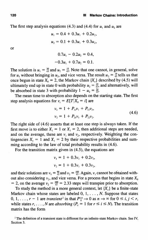
120 III Markov Chains: Introduction
The first step analysis equations (4.3) and (4.4) for u, and u, are
u, = 0.4 + 0.3u, + 0.2u,,
u, = 0.1 + 0.3u, + 0.3u,,or
0.7u, - 0.2u, = 0.4,
-0.3u, + 0.7u, = 0.1.
The solution is u, = ° 4and u, _9. Note that one cannot, in general, solvefor u, without bringing in u,, and vice versa. The result u, = ',; tells us thatonce begun in state Xo = 2, the Markov chain described by (4.5) will
13 , and alternatively, willultimately end up in state 0 with probability u, =be absorbed in state 3 with probability I - u, =41.
The mean time to absorption also depends on the starting state. The firststep analysis equations for v; = E[TI XO = i] are
v, = I + P,,v,,
v, = 1 + -',v, +(4.6)
The right side of (4.6) asserts that at least one step is always taken. If thefirst move is to either X, = 1 or X, = 2, then additional steps are needed,and on the average, these are v, and v,, respectively. Weighting the con-tingencies X, = 1 and X, = 2 by their respective probabilities and sum-ming according to the law of total probability results in (4.6).
For the transition matrix given in (4.5), the equations are
v, = 1 + 0.3v, + 0.2v,,
v, = I + 0.3v, + 0.3v,,
and their solutions are v, _ and v, .1A gain, v, cannot be obtained with-43 - 4
out also considering v,, and vice versa. For a process that begins in state Xo= 2, on the average v, = 43= 2.33 steps will transpire prior to absorption.
To study the method in a more general context, let be a finite-stateMarkov chain whose states are labeled 0, 1, . . . , N. Suppose that states0, 1,...,r- 1aretransient2inthat P:.7- 0asn-4oc for0:5 i,j<r,while states r, . . . , N are absorbing (P; = I for r < i !5; N). The transitionmatrix has the form
' The definition of a transient state is different for an infinite-state Markov chain. See IV,Section 3.

4. First Step Analysis 121
P= I '0 '1 [ (4.7)
where 0 is an (N - r + 1) X r matrix all of whose entries are zero, I is an(N - r + 1) X (N - r + 1) identity matrix, and Q;j = Pj for 0 : i, j < r.
Started at one of the transient states X0 = i, where 0 << i < r, sucha process will remain in the transient states for some random duration,but ultimately the process gets trapped in one of the absorbing statesi = r, . . . , N. Functionals of importance are the mean duration until ab-sorption and the probability distribution over the states in which absorp-tion takes place.
Let us consider the second question first and fix a state k among the ab-sorbing states (r : k s N). The probability of ultimate absorption in statek, as opposed to some other absorbing state, depends on the initial stateXo = i. Let Uk = u, denote this probability, where we suppress the targetstate k in the notation for typographical convenience.
We begin a first step analysis by enumerating the possibilities in thefirst transition. Starting from state i, then with probability Pk the processimmediately goes to state k, thereafter to remain, and this is the first pos-sibility considered. Alternatively, the process could move on its first stepto an absorbing state j : k, where r <_ j : N, in which case ultimate ab-sorption in state k is precluded. Finally, the process could move to a tran-sient state j < r. Because of the Markov property, once in state j, then theprobability of ultimate absorption in state k is uj = Uk by definition.Weighting the enumerated possibilities by their respective probabilitiesvia the law of total probability, we obtain the relation
U. = Pr{Absorption in klX0 = i}
Pr{Absorption in kIX0 = i, X, = j}pjj=o
N r-
=Pi Pj=rj*k
j=o
To summarize, for a fixed absorbing state k, the quantities
u; = Uk = Pr{Absorption in klX0 = i } for 0 < i < r

122 III Markov Chains: Introduction
satisfy the inhomogeneous system of linear equationsI.- I
UR=PA+7' P;jUk, i=0, 1,...,r- 1. (4.8)j=0
Example A Maze A white rat is put into the maze shown:
1 __F_770 1
food
2 3 4
8 '
shock5 6
In the absence of learning, one might hypothesize that the rat would movethrough the maze at random; i.e., if there are k ways to leave a compart-ment, then the rat would choose each of these with probability 1/k. As-sume that the rat makes one change to some adjacent compartment at eachunit of time and let X,, denote the compartment occupied at stage n. Wesuppose that compartment 7 contains food and compartment 8 contains anelectrical shocking mechanism, and we ask the probablity that the rat,moving at random, encounters the food before being shocked. The appro-priate transition probability matrix is
0 1 2 3 4 5 6 7 8
0
1
2 2
3 ; 3
3 3
3
3 3
1
1

4. First Step Analysis 123
Let u; = u;(7) denote the probability of absorption in the food compart-ment 7, given that the rat is dropped initially in compartment i. Then equa-tions (4.8) become, in this particular instance,
U0 =Zu,
+ lug,
1 1 I
ul - 3 + 3u0 + 3u3,1 I
U2 = 3uo + 3u31
U3 = 4U1 + 4u2 + 4U4 + 4U5,I 1 I
u4 = 3 + 3u3 + 3u6+
U5 = 1
3u3 +I3u6e
U6 = ?u4 + 12U5-
Turning to the solution, we see that the symmetry of the maze implies thatuo = u6, u2 = u5, and u, = u4. We also must have u3 =!. With these sim-plifications the equations for uo, u and u2 become
U0 = ?ul + ;U2,
u1 = z +13uo+
U,2=6+luo,
and the natural substitutions give uo = ;Z + lu0) +Z(6
+ luo), or uo = ;,_ z 1U, -3, anduz = 3.One might compare these theoretical values under random moves with
actual observations as an indication of whether or not learning is takingplace.
4.2. The General Absorbing Markov Chain
Let (X,, } be a Markov chain whose transition probability matrix takes theform (4.7). We turn to a more general form of the first question by intro-ducing the random absorption time T. Formally, we define
T=min{n? 0;X?r}.

124 III Markov Chains: Introduction
Let us suppose that associated with each transient state i is a rate g(i) andthat we wish to determine the mean total rate that is accumulated up to ab-sorption. Let w, be this mean total amount, where the subscript i denotesthe starting position X0 = i. To be precise, let
T-Iw; = E[ g(X,,)IX0 = i
,1=0
The choice g(i) = 1 for all i yields ,T=o g(X,,) _ T=o 1 = T, and thenw; is identical to v, = E[TIXO = i], the mean time until absorption. For atransient state k, the choice
1 ifi=k,g(i)={0 ifi*k,
gives w, = Wk, the mean number of visits to state k (0 <- k < r) prior toabsorption.
We again proceed via a first step analysis. The sum YT=p alwaysincludes the first term g(X0) = g(i). In addition, if a transition is madefrom i to a transient state j, then the sum includes future terms as well. Byinvoking the Markov property we deduce that this future sum proceedingfrom state j has an expected value equal to w;. Weighting this by the tran-sition probability P, and then summing all contributions in accordancewith the law of total probability, we obtain the joint relations
r-1
w;=g(i)+Y, P,w; for i=0,...,r- 1. (4.9)i=o
The special case in which g(i) = 1 for all i determines v, = E[TI`Xo = i]as solving
1.- 1
v;=1+7, P;v; fori=0,1,...,r-1. (4.10)l=o
The case in which
1 ifi=k,S(i)=Sk={0 ifi0k,
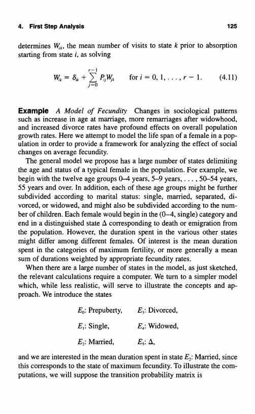
4. First Step Analysis 125
determines Wk, the mean number of visits to state k prior to absorptionstarting from state i, as solving
,.-1
Wk= 6;k+7 P,Wkj=0
fori=0, 1,...,r- 1. (4.11)
Example A Model of Fecundity Changes in sociological patternssuch as increase in age at marriage, more remarriages after widowhood,and increased divorce rates have profound effects on overall populationgrowth rates. Here we attempt to model the life span of a female in a pop-ulation in order to provide a framework for analyzing the effect of socialchanges on average fecundity.
The general model we propose has a large number of states delimitingthe age and status of a typical female in the population. For example, webegin with the twelve age groups 0-4 years, 5-9 years, . . . , 50-54 years,55 years and over. In addition, each of these age groups might be furthersubdivided according to marital status: single, married, separated, di-vorced, or widowed, and might also be subdivided according to the num-ber of children. Each female would begin in the (0-4, single) category andend in a distinguished state A corresponding to death or emigration fromthe population. However, the duration spent in the various other statesmight differ among different females. Of interest is the mean durationspent in the categories of maximum fertility, or more generally a meansum of durations weighted by appropriate fecundity rates.
When there are a large number of states in the model, as just sketched,the relevant calculations require a computer. We turn to a simpler modelwhich, while less realistic, will serve to illustrate the concepts and ap-proach. We introduce the states
E0: Prepuberty, E,: Divorced,
E,: Single, E,: Widowed,
E,: Married, Es: A,
and we are interested in the mean duration spent in state E,: Married, sincethis corresponds to the state of maximum fecundity. To illustrate the com-putations, we will suppose the transition probability matrix is

126 III Markov Chains: Introduction
Eo E, E2 E3 E, E5
Eo 0 0.9 0 0 0 0.1
E, 0 0.5 0.4 0 0 0.1
E2 0 0 0.6 0.2 0.1 0.1P =
E3 0 0 0.4 0.5 0 0.1
E, 0 0 0.4 0 0.5 0.1
E5 0 0 0 0 0 1.0
In practice, such a matrix would be estimated from demographic data.Every person begins in state Eo and ends in state E5, but a variety of in-
tervening states may be visited. We wish to determine the mean durationspent in state E2: Married. The powerful approach of first step analysis be-gins by considering the slightly more general problem in which the initialstate is varied. Let w; = W,,2 be the mean duration in state E2 given the ini-tial state X, = E; for i = 0, 1, . . . , 5. We are interested in wo, the mean du-ration corresponding to the initial state E0.
First step analysis breaks down, or analyzes, the possibilities arising inthe first transition, and using the Markov property, an equation that relatesw0, . . . , w5 results.
We begin by considering wo. From state E0, a transition to one of thestates E, or E5 occurs, and the mean duration spent in E2 starting from Eomust be the appropriately weighted average of w, and w5. That is,
wa = 0.9w, + 0.1w5.
Proceeding in a similar manner, we obtain
w, = 0.5w, + 0.4w2 + O.lw5.
The situation changes when the process begins in state E2, because incounting the mean duration spent in E2, we must count this initial visitplus any subsequent visits that may occur. Thus for E2 we have
w2= 1 +0.6w2+0.2w3+0.1w,+0.1w5.
The other states give us
W3=0.4w,+0.5W3+O.IW51
w4 =0.4w2+0.5w,+0.1w5,
w5=w5.
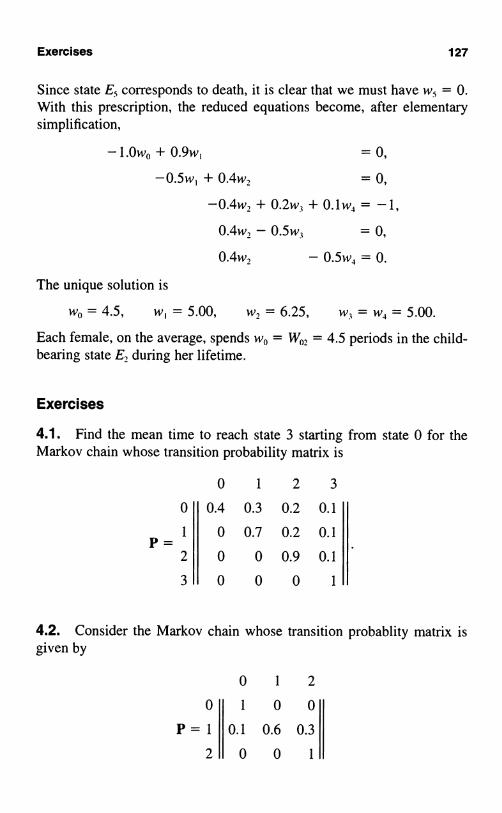
Exercises 127
Since state E., corresponds to death, it is clear that we must have w, = 0.With this prescription, the reduced equations become, after elementarysimplification,
-1.0w + 0.9w, = 0,
-0.5w, + 0.4w, = 0,
-0.4w,+0.2w1+0.1w4= -1,
0.4w, - 0.5w, = 0,
0.4w, -0.5w,=0.
The unique solution is
wo=4.5, w,=5.00, w, = 6.25, w3=w,=5.00.
Each female, on the average, spends w, = W02 = 4.5 periods in the child-bearing state E, during her lifetime.
Exercises
4.1. Find the mean time to reach state 3 starting from state 0 for theMarkov chain whose transition probability matrix is
0 1 2 3
0 0.4 0.3 0.2 0.1
1
0 0.7 0.2 0.1P-2 0 0 0.9 0.1
3 0 0 0 1
4.2. Consider the Markov chain whose transition probablity matrix isgiven by
0 1 2
0 1 0 0
P=1 0.1 0.6 0.3
2 0 0 1

128 III Markov Chains: Introduction
(a) Starting in state 1, determine the probability that the Markov chainends in state 0.
(b) Determine the mean time to absorption.
4.3. Consider the Markov chain whose transition probability matrix isgiven by
0 1 2 3
1 0 0 0
1 0 1 0 6 0 1 0 2P_ . . . .
2 0.2 0.3 0.4 0.1
3 0 0 0 1
(a) Starting in state 1, determine the probability that the Markov chainends in state 0.
(b) Determine the mean time to absorption.
4.4. A coin is tossed repeatedly until two successive heads appear. Findthe mean number of tosses required.
Hint: Let X,, be the cumulative number of successive heads. The statespace is 0, 1, 2 and the transition probability matrix is
Determine the mean time to reach state 2 starting from state 0 by invok-ing a first step analysis.
4.5. A coin is tossed repeatedly until either two successive heads appearor two successive tails appear. Suppose the first coin toss results in a head.Find the probability that the game ends with two successive tails.

Exercises 129
4.6. Consider the Markov chain whose transition probability matrix isgiven by
0 1 2 3
0 1 0 0 0
1 10 40 10 40P_ . . . .
2 0.2 0.1 0.6 0.1
3 0 0 0 1
(a) Starting in state 1, determine the probability that the Markov chainends in state 0.
(b) Determine the mean time to absorption.
4.7. Consider the Markov chain whose transition probability matrix isgiven by
0 1 2 3
0 1 0 0 0
1 0 1 20 0 5 20P=
. . . .
2 0.1 0.2 0.6 0.1
3 0 0 0 1
Starting in state 1, determine the mean time that the process spends instate 1 prior to absorption and the mean time that the process spends instate 2 prior to absorption. Verify that the sum of these is the mean timeto absorption.
4.8. Consider the Markov chain whose transition probability matrix isgiven by
0 1 2 3
0 1 0 0 0
0.5 0.2 0.1 0.2P
2 0.2 0.1 0.6 0.1
3 0 0 0 1

130 III Markov Chains: Introduction
Starting in state 1, determine the mean time that the process spends instate 1 prior to absorption and the mean time that the process spends instate 2 prior to absorption. Verify that the sum of these is the mean timeto absorption.
4.9. Consider the Markov chain whose transition probability matrix isgiven by
0 1 2 3
0 1 0 0 0
1 0 1 20 0 5 20P_ . . . .
2 0.1 0.2 0.6 0.1
3 0 0 0 1
Starting in state 1, determine the probability that the process is absorbedinto state 0. Compare this with the (1,0)th entry in the matrix powers P-,P4, P8, and P's.
Problems
4.1. Which will take fewer flips, on average: successively flipping aquarter until the pattern HHT appears, that is, until you observe two suc-cessive heads followed by a tails; or successively flipping a quarter untilthe pattern HTH appears? Can you explain why these are different?
4.2. A zero-seeking device operates as follows: If it is in state m at timen, then at time n + 1, its position is uniformly distributed over the states0, 1, . . . , m - 1. Find the expected time until the device first hits zerostarting from state m.
Note: This is a highly simplified model for an algorithm that seeks amaximum over a finite set of points.
4.3. A zero-seeking device operates as follows: If it is in state j at timen, then at time n + 1, its position is 0 with probability 1/j, and its positionis k (where k is one of the states 1, 2, . . . , j - 1) with probability 2k/j2.Find the expected time until the device first hits zero starting from state m.

Problems 131
4.4. Consider the Markov chain whose transition probability matrix isgiven by
0 1 2 3
0 1 0 0 0
0.1 0.2 0.5 0.2P
2 0.1 0.2 0.6 0.1
0.2 0.2 0.3 0.3
Starting in state X0 = 1, determine the probability that the process nevervisits state 2. Justify your answer.
4.5. A white rat is put into compartment 4 of the maze shown here:
1 23
food
4 5 6
7
shock
He moves through the compartments at random; i.e., if there are k ways toleave a compartment, he chooses each of these with probability 1/k. Whatis the probability that the rat finds the food in compartment 3 before feel-ing the electric shock in compartment 7?
4.6. Consider the Markov chain whose transition matrix is
0 1 2 3 4
0 q p 0 0 0
1 q 0 p 0 0P= 2
g 0 0 p 0
3 q 0 0 0 p
4 0 0 0 0 1

132 III Markov Chains: Introduction
where p + q = 1. Determine the mean time to reach state 4 starting fromstate 0. That is, find E[TIXO = 0] where T = min{n ? 0; X,, = 4}.
Hint: Let v, = E[TIXO = i] for i = 0, 1, . . . , 4. Establish equationsfor v0, v...... v4 by using a first step analysis and the boundary condi-tion v4 = 0. Then solve for v0.
4.7. Let X,, be a Markov chain with transition probabilities P,. We aregiven a "discount factor" 8 with 0 < P < 1 and a cost function c(i), andwe wish to determine the total expected discounted cost starting from statei, defined by
r x lh; = EI mcm')!Xa = it
Using a first step analysis, show that h, satisfies the system of linearequations
h; = c(i) + 0 P;h; for all states i.
4.8. An urn contains five red and three green balls. The balls are chosenat random, one by one, from the urn. If a red ball is chosen, it is removed.Any green ball that is chosen is returned to the urn. The selection processcontinues until all of the red balls have been removed from the urn. Whatis the mean duration of the game?
4.9. An urn contains five red and three yellow balls. The balls are chosenat random, one by one, from the urn. Each ball removed is replaced in theurn by a yellow ball. The selection process continues until all of the red ballshave been removed from the urn. What is the mean duration of the game?
4.10. You have five fair coins. You toss them all so that they randomlyfall heads or tails. Those that fall tails in the first toss you pick up and tossagain. You toss again those that show tails after the second toss, and so on,until all show heads. Let X be the number of coins involved in the lasttoss. Find Pr(X = 1).
4.11. An urn contains two red and two green balls. The balls are chosenat random, one by one, and removed from the urn. The selection process

Problems 133
continues until all of the green balls have been removed from the urn.What is the probability that a single red ball is in the urn at the time thatthe last green ball is chosen?
4.12. A Markov chain X0, X, , X,.... has the transition probabilitymatrix
0 1 2
0 0.3 0.2 0.5
P=1 0.5 0.1 0.4
2 0 0 1
and is known to start in state X0 = 0. Eventually, the process will end upin state 2. What is the probability that when the process moves into state2, it does so from state 1?
Hint: Let T = min(n ? 0; X,, = 2), and let
z; = Pr{XT_, = 1IX0 = i) for i = 0, 1.
Establish and solve the first step equations
zo = 0.3zo + 0.2z
z,=0.4+0.5z()+O.lz,.
4.13. A Markov chain X,,, X,, X,.... has the transition probabilitymatrix
0 1 2
0 0.3 0.2 0.5
P=1 0.5 0.1 0.4
2 0 0 1
and is known to start in state X = 0. Eventually, the process will end upin state 2. What is the probability that the time T = min{n > 0; X,, = 2}is an odd number?

134 III Markov Chains: Introduction
4.14. A single die is rolled repeatedly. The game stops the first time thatthe sum of two successive rolls is either 5 or 7. What is the probability thatthe game stops at a sum of 5?
4.15. A simplified model for the spread of a rumor goes this way: Thereare N = 5 people in a group of friends, of which some have heard therumor and the others have not. During any single period of time, two peo-ple are selected at random from the group and assumed to interact. The se-lection is such that an encounter between any pair of friends is just aslikely as between any other pair. If one of these persons has heard therumor and the other has not, then with probability a = 0.1 the rumor istransmitted. Let X,, denote the number of friends who have heard therumor at the end of the nth period.
Assuming that the process begins at time 0 with a single person know-ing the rumor, what is the mean time that it takes for everyone to hear it?
4.16. An urn contains 5 tags, of which 3 are red and 2 are green. A tagis randomly selected from the urn and replaced with a tag of the oppositecolor. This continues until only tags of a single color remain in the urn.Let X denote the number of red tags in the urn after the nth draw, withXo = 3. What is the probability that the game ends with the urn contain-ing only red balls?
4.17. The damage X of a system subjected to wear is a Markov chainwith the transition probability matrix
0 1 2
0 0.7 0.3 0
P=1 0 0.6 0.4
2 0 0 1
The system starts in state 0 and fails when it first reaches state 2. LetT = min( n ? 0; X = 2) be the time of failure. Use a first step analysis toevaluate ¢(s) = E[sn ] for a fixed number 0 < s < 1. (This is called thegenerating function of T. See Section 9.)
4.18. Time-dependent transition probabilities. A well-disciplinedman, who smokes exactly one half of a cigar each day, buys a box con-

5. Some Special Markov Chains 135
taining N cigars. He cuts a cigar in half, smokes half, and returns the otherhalf to the box. In general, on a day in which his cigar box contains wwhole cigars and h half cigars, he will pick one of the w + h smokes atrandom, each whole and half cigar being equally likely, and if it is a halfcigar, he smokes it. If it is a whole cigar, he cuts it in half, smokes onepiece, and returns the other to the box. What is the expected value of T,the day on which the last whole cigar is selected from the box?
Hint: Let X,, be the number of whole cigars in the box after the nthsmoke. Then X is a Markov chain whose transition probabilities varywith n. Define v (w) = E[T I X,, = w]. Use a first step analysis to developa recursion for v (w) and show that the solution is
2Nw+n+2w IA I
whence
w + 1
E[T] = vo(N) = 2N -
4.19. Computer Challenge. Let N be a positive integer and letZ . . . , Z be independent random variables, each having the geometricdistribution
111Pr{Z=k} =(2I, fork= 1,2.....
Since these are discrete random variables, the maximum among them maybe unique, or there may be ties for the maximum. Let p,,, be the probabil-ity that the maximum is unique. How does p,,, behave when N is large? (Al-ternative formulation: You toss N dimes. Those that are heads you setaside; those that are tails you toss again. You repeat this until all of thecoins are heads. Then p, is the probability that the last toss was of a sin-gle coin.)
5. Some Special Markov Chains
We introduce several particular Markov chains that arise in a variety ofapplications.

136
5.1. The Two-State Markov Chain
Let
P=0
III Markov Chains: Introduction
where 0 < a, b < 1, (5.1)
be the transition matrix of a two-state Markov chain.When a = 1 - b, so that the rows of P are the same, then the states
X, X 2,.. . are independent identically distributed random variables withPr(X,, = 0) = b and Pr(X = 1) = a. When a 0 1 - b, the probability dis-tribution for X,, varies depending on the outcome at the previous stage.
For the two-state Markov chain, it is readily verified by induction thatthe n-step transition matrix is given by
P"= 1 b a
b a
+ (1 - a - b)"a+b
a -a-b b
To verify this general formula, introduce the abbreviations
A= b a
b aand B =
a -a-b b
so that (5.2) can be written
P (a+b)-'[A+(1 -a-b)"B)Next, check the multiplications
AP =
and
BP =
b a
b a
0 1
1-a a
b 1-b
a+b
x
a -a-b b
1-a a
b 1-b
x1-a a
b 1 -b
b a
b a=A
(5.2)
_ a-a2-ab a2-a+ab- I -b+ab+bz -ab+b-b''11 =(1-a-b)B.

5. Some Special Markov Chains 137
Now (5.2) is easily seen to be true when n = 1, since then
1
P' =a+b
b a
b a
+(1-a-b)a+b
a -a
-b b
b+a-a2-ab a-a+a2+abb-b+ab+b22 a+b-ab-b2
1-a a
b 1-b = P.
To complete an induction proof, assume that the formula is true for n.Then
P"P = (a + b)-'[A + (1 - a - b)"B]P
= (a + b)-'[AP + (1 - a - b)"BP]=(a+b)-'[A+(1 -a-b)"+'B] = P"
We have verified that the formula holds for n + 1. It therefore is estab-lished for all n.
Note that 11 -a-bj<1 when 0 < a, b < 1, and thus 11 -a-b("- 0as n -3 and
lim P" ="-Ix
(5.3)
This tells us that such a system, in the long run, will be in state 0 withprobability b/(a + b) and in state 1 with probability a/(a + b), irrespec-tive of the initial state in which the system started.
For a numerical example, suppose that the items produced by a certainworker are graded as defective or not, and that due to trends in raw mate-rial quality, whether or not a particular item is defective depends in parton whether or not the previous item was defective. Let X,, denote the qual-ity of the nth item with X,, = 0 meaning "good" and X,, = 1 meaning "de-fective." Suppose that {X } evolves as a Markov chain whose transitionmatrix is

138 III Markov Chains: Introduction
P=00 1
0.99 0.010.12 0.88
Defective items would tend to appear in bunches in the output of such asystem.
In the long run, the probability that an item produced by this system isdefective is given by al(a + b) = 0.01/(0.01 + 0.12) = 0.077.
5.2. Markov Chains Defined byIndependent Random Variables
Let denote a discrete-valued random variable whose possible values arethe nonnegative integers and where Pr{4 = i } = a; ? 0, for i = 0, 1, ... ,and , U a; = 1. Let 6,, 6,, ... , 6,,, ... represent independent observa-tions of .
We shall now describe three different Markov chains connected withthe sequence ,, 6,..... In each case the state space of the process is theset of nonnegative integers.
Example Independent Random Variables Consider the process X,,,n = 0, 1, 2, ... , defined by X,, (X,, _ o prescribed). Its Markov ma-trix has the form
P= (5.4)
That all rows are identical plainly expresses the fact that the random vari-able is independent of X,,.
Example Successive Maxima The partial maxima of 6 ,, ... definea second important Markov chain. Let
for n = 1, 2,. ..,

5. Some Special Markov Chains 139
with 00 = 0. The process defined by X,, = 0,, is readily seen to be a Markovchain, and the relation max { X,,, allows the transition proba-bilities to be computed to be
Ao a, a2 a3
0 A, a2 a3
P= 0 0 A2 a3 (5.5)
0 0 0 A3
where Ak = ao + + a, for k = 0, 1, ... .Suppose ,, 2, ... represent successive bids on a certain asset that is of-
fered for sale. Then X = max { . . . , &) is the maximum that is bid upto stage n. Suppose that the bid that is accepted is the first bid that equalsor exceeds a prescribed level M. The time of sale is the random variableT = min{n >_ 1; X,, ? M}. A first step analysis shows that the meanµ = E[T] satisfies
A = 1 + A M}, (5.6)
or µ = 1/Pr{e, >_ M} = 1/(a,,, + a,,,+, + ). The first step analysis in-voked in establishing (5.6) considers the two possibilities {6, < M} and{6, > M}. With this breakdown, the law of total probability justifies thesum
E[T] = MI M) + E[Tle, < M] M}. (5.7)
Clearly, E[TI , ? MI = 1, since no further bids are examined in this case.On the other hand, when , < M we have the first bid, which was not ac-cepted, plus some future bids. The future bids 2, 3, . . . have the same prob-abilistic properties as in the original problem, and they are examined untilthe first acceptable bid appears. This reasoning leads to E[TI , < M] _1 + µ. Substitution into (5.7) then yields (5.6) as follows:
E[T] = 1 X Pr{6, ? M} + (1 + µ) M}
= I +µPr{6, <M}.
To restate the argument somewhat differently, one always examines thefirst bid 6,. If , < M, then further bids are examined in a future that is

140 III Markov Chains: Introduction
probabilistically similar to the original problem. That is, when 6, < M,then on the average µ bids in addition to 6, must be examined before anacceptable bid appears. Equation (5.6) results.
Example Partial Sums Another important Markov chain arises fromconsideration of the successive partial sums i' of the ;, i.e.,
n1,2,...,and by definition, 77, = 0. The process X,, = rl is readily seen to be aMarkov chain via
jIX, = i ... , i)
= Pr{ +I - .l - 4 1 = il, 62 = l2 - i,, . . . , 6,, = i - i,,_1}
= j - i} (independence of 6,, 2, ...)
=Pr{Xi+1=jlX,, =i}.
The transition probability matrix is determined by
Pr{ ,+, = j - i}
_ jaj-i for j ? i,0 for j < i,
where we have used the independence of the 6;.Schematically, we have
P=
ao a, a, a3
0 ao a, a2
0 0 ao a,
(5.8)
If the possible values of the random variable 6 are permitted to be thepositive and negative integers, then the possible values of rl,, for each nwill be contained among the totality of all integers. Instead of labeling thestates conventionally by means of the nonnegative integers, it is more con-venient to identify the state space with the totality of integers, since the

S. Some Special Markov Chains 141
transition probability matrix will then appear in a more symmetric form.The state space consists then of the values ... -2, -1, 0, 1, 2, ...The transition probability matrix becomes
P=a_,
a-,
ao
a-,
a,
ao
a,
a, a,
a-3 a_, a_, ao a,
where Pr{ = k} = a k for k = 0, ±1, ±2, ... ,and ak L-0, 1:k=_= ak = 1.
5.3. One-Dimensional Random Walks
When we discuss random walks, it is an aid to intuition to speak about thestate of the system as the position of a moving "particle."
A one-dimensional random walk is a Markov chain whose state spaceis a finite or infinite subset a, a + 1, . . . , b of the integers, in which theparticle, if it is in state i, can in a single transition either stay in i or moveto one of the neighboring states i - 1, i + 1. If the state space is taken asthe nonnegative integers, the transition matrix of a random walk has theform
0
1
P= 2
i
0 1 2 i-1 i i+lro Po 0 ... 0 ...
q, r, P, ... 0 ...0 q2 r2 0 ...
0 q; r; p, 0
(5.9)
where p,>O,q;>0,r,?O,and q;+r;+p;= 1,i= 1,2,...(i? 1),po ? 0, ro ? 0, ro + po = 1. Specifically, if X,, = i, then for i ? 1,

142 III Markov Chains: Introduction
i + 1 X,, = i} = p;,
=q;,
with the obvious modifications holding for i = 0.The designation "random walk" seems apt, since a realization of the
process describes the path of a person (suitably intoxicated) moving ran-domly one step forward or backward.
The fortune of a player engaged in a series of contests is often depictedby a random walk process. Specifically, suppose an individual (player A)with fortune k plays a game against an infinitely rich adversary and hasprobability pk of winning one unit and probability qk = 1 - p, (k ? 1) oflosing one unit in the next contest (the choice of the contest at each stagemay depend on his fortune), and ro = 1. The process X,,, where X,, repre-sents his fortune after n contests, is clearly a random walk. Note that oncethe state 0 is reached (i.e., player A is wiped out), the process remains inthat state. The event of reaching state k = 0 is commonly known as the"gambler's ruin."
If the adversary, player B, also starts with a limited fortune l and playerA has an initial fortune k (k + l = N), then we may again consider theMarkov chain process X,, representing player A's fortune. However, thestates of the process are now restricted to the values 0, 1, 2, . . . , N. At anytrial, N - X,, is interpreted as player B's fortune. If we allow the possibil-ity of neither player winning in a contest, the transition probability matrixtakes the form
0 1 2 3 N
1 0 0 0 ...q, r, PI 0 ...0 q2 r,
P2...
qN-I rN-I PN-1
N 0 0 0 1
(5.10)
Again p; (q;), i = 1, 2, . . . , N - 1, denotes the probability of player A'sfortune increasing (decreasing) by 1 at the subsequent trial when his

5. Some Special Markov Chains 143
present fortune is i, and r, may be interpreted as the probability of a draw.Note that, in accordance with the Markov chain given in (5.10), whenplayer A's fortune (the state of the process) reaches 0 or N it remains inthis same state forever. We say player A is ruined when the state of theprocess reaches 0, and player B is ruined when the state of the processreaches N.
The probability of gambler's ruin (for player'A) is derived in the nextsection by solving a first step analysis. Some more complex functionals onrandom walk processes are also derived there.
The random walk corresponding to Pk = p, qk = 1 - p = q for allk ? 1 and ro = I describes the situation of identical contests. There is adefinite advantage to player A in each individual trial if p > q, and con-versely, an advantage to player B if p < q. A "fair" contest corresponds top = q = ;. Suppose the total of both players' fortunes is N. Then the cor-responding walk, where X,, is player A's fortune at stage n, has the transi-tion probability matrix
0
1
P=2
N-1N
0 1 2 3 N-1 N1 0 0 0 0 0
g 0 p 0 .. 0 0
0 g 0 p .. 0 0
0 0 0 0 0 p
0 0 0 0 ... 0 1
(5.11)
Let u; = U,0 be the probability of gambler's ruin starting with the initialfortune i. Then u, is the probability that the random walk reaches state 0before reaching state N, starting from X. = i. The first step analysis of Sec-tion 4, as used in deriving equation (4.8), shows that these ruin probabil-ities satisfy
u; = pu,+, + qu;_, for i = 1, ... , N - 1 (5.12)
together with the obvious boundary conditions
uo = 1 and UN = 0.
These equations are solved in the next section following a straight-forward but arduous method. There it is shown that the gambler's ruin

144 III Markov Chains: Introduction
probabilities corresponding to the transition probability matrix given in(5.11) are
u; = Pr{X reaches state 0 before state IVIX, = i}
when p=q=Z,
whenp 0 q.(5.13)
The ruin probabilities u; given by (5.13) have the following interpreta-tion. In a game in which player A begins with an initial fortune of i unitsand player B begins with N - i units, the probability that player A losesall his money before player B goes broke is given by u,, where p is theprobability that player A wins in a single contest. If player B is infinitelyrich (N - cc), then passing to the limit in (5.13) and using (q/p)" -4 00 asN -+ oo if p < q, while (q/p)" -4 0 if p > q, we see that the ruin probabil-ities become
if psq,if p > q. (5.14)
(In passing to the limit, the case p = q = z must be treated separately.) Wesee that ruin is certain (u; = 1) against an infinitely rich adversary whenthe game is unfavorable (p < q), and even when the game is fair (p = q).In a favorable game (p > q), starting with initial fortune i, then ruin oc-curs (player A goes broke) with probability (q/p)'. This ruin probability de-creases as the initial fortune i increases. In a favorable game against an in-finitely rich opponent, with probability 1 - (q/p)' player A's fortuneincreases, in the long run, without limit.
More complex gambler's-ruin-type problems find practical relevance incertain models describing the fluctuation of insurance company assetsover time.
Random walks are not only useful in simulating situations of gamblingbut frequently serve as reasonable discrete approximations to physicalprocesses describing the motion of diffusing particles. If a particle is sub-

5. Some Special Markov Chains 145
jected to collisions and random impulses, then its position fluctuates ran-domly, although the particle describes a continuous path. If the future po-sition (i.e., its probability distribution) of the particle depends only on thepresent position, then the process X where X, is the position at time t, isMarkov. A discrete approximation to such a continuous motion corre-sponds to a random walk. A classical discrete version of Brownian motion(VIII) is provided by the symmetric random walk, By a symmetric ran-dom walk on the integers (say all the integers) we mean a Markov chainwith state space the totality of all integers and whose transition probabil-ity matrix has the elements
P lt]=t+1,
P; _p ifj=i - 1,r ifj=i,0 otherwise,
i,j=0,1,2,...,
where p > 0, r ? 0, and 2p + r = 1. Conventionally, "simple randomwalk" refers only to the case r = 0, p = Z.
The classical simple random walk in n dimensions admits the follow-ing formulation. The state space is identified with the set of all integrallattice points in E' (Euclidean n space); that is, a state is an n-tuple k =(k,, k,, ... , of integers. The transition probability matrix is defined by
I4-k,l = 1,i=o
otherwise.
Analogous to the one-dimensional case, the simple random walk in E'represents a discrete version of n-dimensional Brownian motion.
5.4. Success Runs
Consider a Markov chain on the nonnegative integers with transitionprobability matrix of the form

146 III Markov Chains: Introduction
0 1 2 3 4
0 po qo 0 0 0
1 p, r, q, 0 0
P= 2 P2 0 r, q2 0 (5.15)
3 p3 0 0 r3 q3
where q; > 0, p; > 0, and p, + q, + r; = 1 for i = 0, 1, 2, .... The zerostate plays a distinguished role in that it can be reached in one transitionfrom any other state, while state i + 1 can be reached only from state i.
This example arises surprisingly often in applications and at the sametime is very easy to compute with. We will frequently illustrate conceptsand results in terms of it.
A special case of this transition matrix arises when one is dealing withsuccess runs resulting from repeated trials each of which admits two pos-sible outcomes, success S or failure F. More explicitly, consider a se-quence of trials with two possible outcomes S or F. Moreover, supposethat in each trial, the probability of S is a and the probability of F is0 = 1 - a. We say a success run of length r happened at trial n if the out-comes in the preceding r + 1 trials, including the present trial as the last,were respectively F, S, S, . . . , S. Let us now label the present state of theprocess by the length of the success run currently under way. In particu-lar, if the last trial resulted in a failure, then the state is zero. Similarly,when the preceding r + 1 trials in order have the outcomes F, S, S, ... ,S, the state variable would carry the label r. The process is clearly Markov(since the individual trials were independent of each other), and its transi-tion matrix has the form (5.15), where
p,, /3, r,,= 0, and q = a for n = 0, 1, 2, ... .
A second example is furnished by the current age in a renewal process.Consider a light bulb whose lifetime, measured in discrete units, is a ran-dom variable , where
Pr( =k}=a,>0 fork= 1,2,..., a,=1.k=1
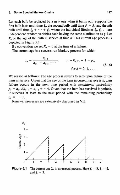
5. Some Special Markov Chains 147
Let each bulb be replaced by a new one when it bums out. Suppose thefirst bulb lasts until time the second bulb until time , + 62, and the nthbulb until time 6, + . + ,,, where the individual lifetimes 2, ... areindependent random variables each having the same distribution as LetX,, be the age of the bulb in service at time n. This current age process isdepicted in Figure 5.1.
By convention we set X,, = 0 at the time of a failure.The current age is a success run Markov process for which
Pk =ak+l
ak+ I+ ak+2 + ...rk=0,qk= 1 Pk+
fork=0,1.....(5.16)
We reason as follows: The age process reverts to zero upon failure of theitem in service. Given that the age of the item in current service is k, thenfailure occurs in the next time period with conditional probabilityPk = ak+1/(ak+I + ak+2 + ). Given that the item has survived k periods,it survives at least to the next period with the remaining probabilityqk = 1 - Pk-
Renewal processes are extensively discussed in VII.
Figure 5.1 The current age X,, in a renewal process. Here f, = 3, 2 = 2,ands,=3.

148 III Markov Chains: Introduction
Exercises
5.1. The probability of the thrower winning in the dice game called"craps" is p = 0.4929. Suppose Player A is the thrower and begins thegame with $5, and Player B, his opponent, begins with $10. What is theprobability that Player A goes bankrupt before Player B? Assume that thebet is $1 per round.
Hint: Use equation (5.13).
5.2. Determine the gambler's ruin probability for Player A when bothplayers begin with $50, bet $1 on each play, and where the win probabil-ity for Player A in each game is
(a) p = 0.49292929(b) p = 0.5029237
(See II, Section 2.)What are the gambler's ruin probabilities when each player begins with$500?
5.3. Determine P" for n = 2, 3, 4, 5 for the Markov chain whose transi-tion probability matrix is
P= 0.4 0.60.7 0.3
5.4. A coin is tossed repeatedly until three heads in a row appear. Let X,,record the current number of successive heads that have appeared. That is,X = 0 if the nth toss resulted in tails; X,, = 1 if the nth toss was heads andthe (n - 1)st toss was tails; and so on. Model X,, as a success runs Markovchain by specifying the probabilities p, and q;.
5.5. Suppose that the items produced by a certain process are eachgraded as defective or good, and that whether or not a particular item isdefective or good depends on the quality of the previous item. To be spe-cific, suppose that a defective item is followed by another defective itemwith probability 0.80, whereas a good item is followed by another gooditem with probability 0.95. Suppose that the initial (zeroth) item is good.Using equation (5.2), determine the probability that the eighth item is

Exercises 149
good, and verify this by computing the eighth matrix power of the transi-tion probability matrix.
5.6. A baseball trading card that you have for sale may be quite valu-able. Suppose that the successive bids ,, i2.... that you receive are in-dependent random variables with the geometric distribution
Pr( = k) = 0.01(0.99)k for k = 0, 1.... .
If you decide to accept any bid over $100, how many bids, on the aver-age, will you receive before an acceptable bid appears?
Hint: Review the discussion surrounding equation (5.6).
5.7. Consider the random walk Markov chain whose transition proba-bility matrix is given by
0 1 2 3
0 1 0 0 0
0.3 0 0.7 0P
2 0 0.3 0 0.7
3 0 0 0 1
Starting in state 1, determine the probability that the process is absorbedinto state 0. Do this first using the basic first step approach of equations(4.3) and (4.4), and second using the particular results for a random walkgiven in equation (5.13).
5.8. As a special case, consider a discrete-time queueing model inwhich at most a single customer arrives in any period and at most a singlecustomer completes service. Suppose that in any single period, a singlecustomer arrives with probability a, and no customers arrive with proba-bility 1 - a. Provided that there are customers in the system, in a singleperiod a single customer completes service with probability f3, and no cus-tomers leave with probability 1 - (3. Then X,,, the number of customers inthe system at the end of period n, is a random walk in the sense of Section5.3. Referring to equation (5.9), specify the transition probabilities p;, q;,and r; for i = 0,1.....

150 III Markov Chains: Introduction
5.9. In a simplified model of a certain television game show, supposethat the contestant, having won k dollars, will at the next play have k + 1dollars with probability q and be put out of the game and leave with noth-ing with probability p = 1 - q. Suppose that the contestant begins withone dollar. Model her winnings after n plays as a success runs Markovchain by specifying the transition probabilities p;, q;, and r; in equation(5.15).
Problems
5.1. As a special case of the successive maxima Markov chain whosetransition probabilities are given in equation (5.5), consider the Markovchain whose transition probability matrix is given by
0 1 2 3
0 ao a, a, a3
1 0 ao + a, a2 a3P=
2 0 0 ao + a, + a2 a3
3 0 0 0 1
Starting in state 0, show that the mean time until absorption is vo = 1/a3.
5.2. A component of a computer has an active life, measured in discreteunits, that is a random variable T, where Pr{T = k} = a,, for k = 1, 2.... .
Suppose one starts with a fresh component, and each component is re-placed by a new component upon failure. Let X,, be the age of the compo-nent in service at time n. Then is a success runs Markov chain.
(a) Specify the probabilities p; and q,.(b) A "planned replacement" policy calls for replacing the component
upon its failure or upon its reaching age N, whichever occurs first.Specify the success runs probabilities p; and q; under the plannedreplacement policy.
5.3. A Batch Processing Model. Customers arrive at a facility andwait there until K customers have accumulated. Upon the arrival of theKth customer, all are instantaneously served, and the process repeats. Let

6. Functionals of Random Walks and Success Runs 151
eo, e . . . denote the arrivals in successive periods, assumed to be inde-pendent random variables whose distribution is given by
Pr{6,=0}=a, 1} = 1 -a,where 0 < a < 1. Let X,, denote the number of customers in the system attime n. Then is a Markov chain on the states 0, 1, . . . , K - 1. WithK = 3, give the transition probability matrix for Be explicit aboutany assumptions you make.
5.4. Martha has a fair die with the usual six sides. She throws the dieand records the number. She throws the die again and adds the secondnumber to the first. She repeats this until the cumulative sum of all thetosses first exceeds 10. What is the probability that she stops at a cumula-tive sum of 13?
5.5 Let be a random walk for which zero is an absorbing state andsuch that from a positive state, the process is equally likely to go up ordown one unit. The transition probability matrix is given by (5.9) withr0 = 1 and p, = q; = ; for i ? 1. (a) Show that is a nonnegative mar-tingale. (b) Use the maximal inequality II, (5.7) to limit the probabilitythat the process ever gets as high as N > 0.
6. Functionals of Random Walks and Success Runs
Consider first the random walk on N + 1 states whose transition proba-bility matrix is given by
0
1
P= 2
0 1 2 3 N
1 0 0 0 0
g 0 p 0 0
0 g 0 p 0
NII0 0 0 0 1
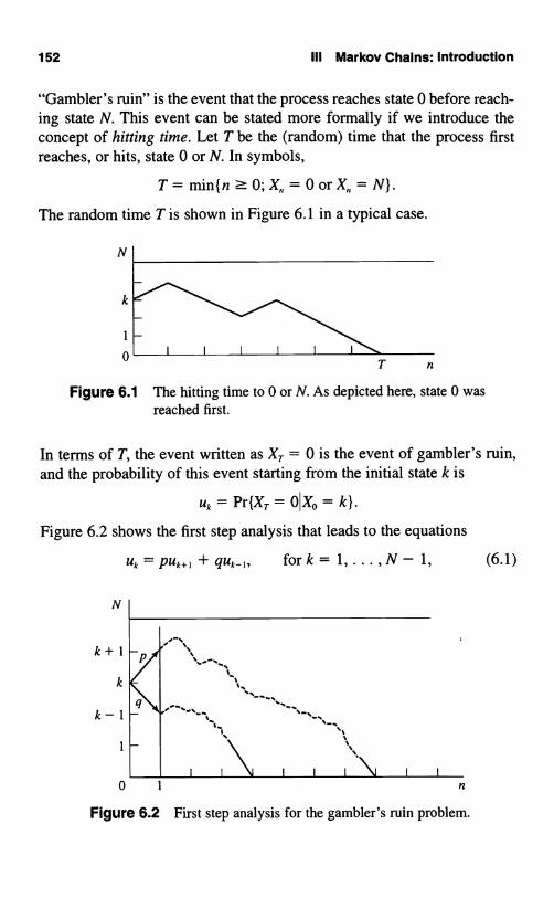
152 III Markov Chains: Introduction
"Gambler's ruin" is the event that the process reaches state 0 before reach-ing state N. This event can be stated more formally if we introduce theconcept of hitting time. Let T be the (random) time that the process firstreaches, or hits, state 0 or N. In symbols,
T=min{n?O;X,, =0or
The random time T is shown in Figure 6.1 in a typical case.
Figure 6.1 The hitting time to 0 or N. As depicted here, state 0 wasreached first.
In terms of T, the event written as X, = 0 is the event of gambler's ruin,and the probability of this event starting from the initial state k is
uk = Pr{X, = OjXO = k}.
Figure 6.2 shows the first step analysis that leads to the equations
uk=Puk+, +quk_ fork= 1,...,N- 1, (6.1)
N
k+1
k
k-1
1
I I I I I `' V I I
0 1 n
Figure 6.2 First step analysis for the gambler's ruin problem.

6. Functionals of Random Walks and Success Runs 153
with the obvious boundary conditions
uo = 1, uN = 0.
Equations (6.1) yield to straightforward but tedious manipulations. Be-cause the approach has considerable generality and arises frequently, it iswell worth pursuing in this simplest case.
We begin the solution by introducing the differences xk = uk - u,-, fork = 1, . . . , N. Using p + q = 1 to write uk = (p + q)uk = PUk + quk,equations (6.1) become
k= 1; 0=p(u2-u1)-q(u,-uo)=px2-qx1;k = 2; 0 = Plus - u2) - q(u2 - u) = Px3 - qx2;
k = 3; 0 = P(u4 - u) - q(u3 - u2) = Px4 - qx3;
k = N - 1; 0 = P(UN - UN-1) q(UN-1 - UN-2) = PXN qxN-1;
or
x2 = (q/P)x1,
x3 = (q/P)x2 = (q/P)2x1,
x4 = (q/p)x3 = (q/p)3x1
Xk = (q/p)xk-1 = (glp)k-1x1,
XN = (q/p)xN-1 = (q/P)N-1x1
We now recover u0, u ... , uN by invoking the conditions uo = 1, UN = 0and summing the xk's:
X,=U1-UO=U1-1,
x2=u,-u1, x1+x2=u2-1,X3=U3- U2, X, +X2+X3 =U3- 1,
Xk=Uk-Uk_1, X, +... +Xk=Uk - 1,
XN = UN - UN-1 - UN-1, X, + ... + XN = UN - 1 = -1-

154 III Markov Chains: Introduction
The equation for general k gives
Uk=1+x,+x,+ +xk= 1 + x, + (q/p)x, + + (q/p)k-'x, (6.2)
= 1 + [I + (qlp) + . + (glp)A- I ]xi,
which expresses uA in terms of the as yet undetermined x,. But u,,, = 0gives
0 = I + [1 +(qlp)+... +(q/p)"-,lx,,
or
x, =1
I + (qlp) + ... + (qlp) -I ,
which substituted into (6.2) gives
u = 1 -1 + (qlp) + ... + (glp)k-1
A 1 + (qlp) + ... + (qlp)'
The geometric series sums to
k ifp=q=j,
1 + (qlp) + ... + (glp)k- i = 1 - (glp)k
1 - (qlp)if p q,
whence
1 - (k/N) = (N - k)/N when p = q =4i21
ux = 1 - 1 - (glp)k _ (qlp)" - (qlp)" when p 0 q.1 - (glp)N 1 - (q/p)N
(6.3)
A similar approach works to evaluate the mean duration
v; = E[TIXO = i). (6.4)
The time T is composed of a first step plus the remaining steps. With prob-ability p the first step is to state i + 1, and then the remainder, on the

6. Functlonals of Random Walks and Success Runs 155
average, is v,,., additional steps. With probability q the first step is toi - 1 and then, on the average, there are v;_, further steps. Thus for themean duration a first step analysis leads to the equation
v; = 1 + pv;+I + gvi_1 ford = 1, . . . , N - 1. (6.5)
Of course, the game ends in states 0 and N, and thus
V0=O, VN=O.
We will solve equations (6.5) when p = q = 2T he solution for othervalues of p proceeds in a similar manner, and the solution for a generalrandom walk is given later in this section.
Again we introduce the differences xk = vk - vk_1 for k = 1, . . . , N,writing (6.5) in the form
k = 1; -1 =2(V2- VI) - i(VI - Vo)=12x2-12X1;
k=2; -1 =2(V3- V2)-12(V2-V0 =12X3-12X2,
k = 3; - 1 = 2(V4 - V3) 2(V3 - V2) = 2X4 2x3;
k = N - 1; -1 = 2(VN - VN-1) 2(VN-I - VN-2) = 2XN 2XN-I
The right side forms a collapsing sum. Upon adding, we obtain
k=1; -1=2x2-2x1;k=2; -2=2x3-2x1;k = 3; -3 = 12x4 - 2x1;
k=N- 1; -(N- 1)=2xN-12x,.
The general line gives xk = x, - 2(k - 1) for k = 2, 3, ... , N. We returnto the vk's by means of
x1=v,-vo= v,;x2=v2-v,; x,+x2=v2;
X3=V3- V2; X1+X2+x3=V3;
Xk = Vk - Vk-1; XI + ... + Xk = Vk;

156 III Markov Chains: Introduction
or
vk=kv, - 2[1 + 2 + + (k - 1)] =kv, - k(k - 1), (6.6)
which gives Vk in terms of the as yet unknown v,. We impose the bound-ary condition vN, = 0 to obtain 0 = Nv, - N(N - 1) or v, _ (N - 1). Sub-stituting this into (6.6) we obtain
vk = k(N - k), k = 0, 1, ... , N, (6.7)
for the mean duration of the game. Note that the mean duration is great-est for initial fortunes k that are midway between the boundaries 0 and N,as we would expect.
6.1. The General Random Walk
We give the results of similar derivations on the random walk whose tran-sition matrix is
0
0 0 0
3 N
0 0
0 0
0
0 1
1
P= 2
N
where q, >0 andpk >0 fork = 1,...,N- 1. LetT=min(n? 0;X = 0 or X = N) be the hitting time to states 0 and N.
Problems
6.1. The probability of gambler's ruin
u;=Prix, =OIXo=i] (6.8)
satisfies the first step analysis equation
u;=q;u;_,+r;u;+p;u;+, for i = 1, . . . , N - 1,
and
U0= 1, uN=0.

6. Functionals of Random Walks and Success Runs 157
The solution is
Pr + ... + PN-I
u' 1 + PI + P2 + ... + PN-Ii= 1,...,N- 1, (6.9)
where
_ glg2 .. qk
PkPIP2 Pk
k= 1,...,N- 1. (6.10)
6.2. The mean hitting time
vk = E[TIXQ = k] (6.11)
satisfies the equations
Vk = 1 + gkVk-I + rkvk + PkVk+I and vo = VN = 0. (6.12)
The solution is
(DI +... +4)N-1Vk-( 1+p,+...+PN-I)(1+PI+...+Pk-1)
- (4), + + Ik- fork= 1,...,N- 1,where p; is given in (6.10) and
q1 g2PI q,P,-I
(6.13)
=q2...q_+q3 q.+...+ q, + 1
(6.14)PI ... Pi P2 P, P,-1P, Pr
fori = 1,...,N- 1.
6.3. Fix a state k, where 0 < k < N, and let Wk be the mean total visitsto state k starting from i. Formally, the definition is
rT-1
Wk = EI 1{X,, = k}IX0 = iJ, (6.15)n-0
where
1 if X,, =k,={0
if k.

158 III Markov Chains: Introduction
Then Wik satisfies the equations
Wk = Sik + q,W-I.k + riWk + PiW+I.k for i = 1, ... , N - Iand
Wok=WNk=0,where
1 ifi=k,
The solution is
_Sik {0 if i * k.
Wk =
( (1 + ... + Pi-1)(A + ... + PN-1) ( 1
r
1 + -- + PN-1 \gkPk- I
I (1 + . . . + Pi-1)(Pk + - - - + PN-1)L 1+ +pN_1
1
A-1)-)
gkPk-I
Example As a sample calculation of these functionals, we consider thespecial case in which the transition probabilities are the same from row torow. That is, we study the random walk whose transition probability ma-trix is
0 1 2 3 N
0 1 0 0 0 0
1 g r p 0 0
P= 2 0 g r p 0
N 0 0 0 0 1
with p > 0, q > 0, and p + q + r = 1. Let us abbreviate by setting0 = (q/p), and then pk, as defined in (6.10), simplifies according to
k
Pk=glgzgk = 9 =Ok fork= 1,...,N-1.PI Pz . ' Pk P

6. Functionals of Random Walks and Success Runs 159
The probability of gambler's ruin, as defined in (6.8) and evaluated in(6.9), becomes
uk = Pr{XT = OIXO = k}
ek - ON
e
if e = (qlp) = 1.
This, of course, agrees with the answer given in (6.3).We turn to evaluating the mean time
vk=E[TIXo=k] fork= 1,...,N= 1by first substituting p; = 0' into (6.14) to obtain
1 + 1 +...+ 1 )eq qO qe;-1
= 1(ei+e'-,+...+6)q
= 1(1+6+ +e'-')p
when p = q(e = 1),
when p 0 q (e 0 1).
Now observe that
pq,,

160 111 Markov Chains: Introduction
so that (6.13) reduces to
Vk = k (4:D, + ... + (DN-1) - ((')I + ... + (I)k-1). (6.17)N
In order to continue, we need to simplify the terms of the form(D, + + (D,-,. We consider the two cases B = (qlp) = 1 and0 = (qlp) 0 1 separately.
When p = q, or equivalently, 0 = 1, then (D; = ilp, whence1+...+(I-1)I(I-1)
P 2p
which inserted into (6.17) gives
v; = E[TlXo = it
= i N(N 1)1 - i(i2 1)L J (6.18)
N 2p P
i(N - i)= if p = q.
2p
When p = 2, then v, = i(N - i) in agreement with (6.7).When p * q, so that 0 = ql p # 1, then
1(1 - 6`=p1-0
whence
P(1-6)[(1-1)-(0+02+...+61-1)l
I 1
11= p(1 1
0)[(J 1) - 6(11 -e0 1J'
and
v;=E[TIXO=il
p(11 0)[N(1-0) p(11 0)['-(1-6)
c
1 - ONHAl - 0)

6. Functionals of Random Walks and Success Runs 161
when 0 = (qlp) 0 1.Finally, we evaluate Wk, expressed verbally as the mean number of vis-
its to state k starting from X0 = i and defined formally in (6.15). Again weconsider the two cases 0 = (qlp) = 1 and 0 = (qlp) 0 1.
When 0 = 1, then p;=0'=1and (6.16) simplifies to
i(N - k)
Wk._ - k) _ k(N - i)
-k)-( qN9 N
i(N - k) max{o, i - k}qN q
When 0 = (qlp) * 1, then p, = 0' and
Pk + - + PN-1 =
and
1-0'
qPk-( = PPk = p0k.
In this case, (6.16) simplifies to
Wk- (1 - 0')(0k- ON)(_1 l(1-0)(1-0")\p0kl
and
Wk- (1- 0k)(0i- 0") 1 forO<k<i<N.(1 - O)(1 - ON) \pokl
(6.19)
We may write the expression for Wk in a single line by introducing thenotation (i - k) + = max{0, i - k}. Then
for 0 < i:5 k < N,
for O < k < i < N,
W(1 - 0')(1 - ON-k) I - 0(i-k)+
(6.20)k = -P(1-0)(1-ON) P(1-0)

162 III Markov Chains: Introduction
6.2. Cash Management
Short-term cash management is the review and control of a corporation'scash balances, short-term loan balances, and short term marketable secu-rity holdings. The objective is to maintain the smallest cash balances thatare adequate to meet future disbursements. The corporation cashier triesto eliminate idle cash balances (by reducing short-term loans or buyingtreasury bills, for example) but to cover potential cash shortages (by sell-ing treasury bills or increasing short-term loans). The analogous problemfor an individual is to maintain an optimal balance between a checkingand a savings account.
In the absence of intervention, the corporation's cash level fluctuatesrandomly as the result of many relatively small transactions. We modelthis by dividing time into successive, equal length periods, each of shortduration, and by assuming that from period to period, the cash levelmoves up or down one unit, each with probability one-half. Let X be thecash on hand in period n. We are assuming that is the random walkin which
k ± 1I X,, = k} = ;.
The cashier's job is to intervene if the cash level ever gets too low or toohigh. We consider cash management strategies that are specified by two pa-rameters, s and El, where 0 < s < 9. The policy is as follows: If the cashlevel ever drops to zero, then sell sufficient treasury bills to replenish thecash level up to s. If the cash level ever increases up to `l, then invest intreasury bills in order to reduce the cash level to s. A typical sequence ofcash levels when s = 2 and 9' = 5 is depicted in Figure 6.3.
First
CycleSecond
CycleThirdCycle
n
Figure 6.3 Several typical cycles in a cash inventory model.
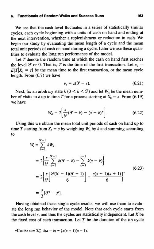
6. Functionals of Random Walks and Success Runs 163
We see that the cash level fluctuates in a series of statistically similarcycles, each cycle beginning with s units of cash on hand and ending atthe next intervention, whether a replenishment or reduction in cash. Webegin our study by evaluating the mean length of a cycle and the meantotal unit periods of cash on hand during a cycle. Later we use these quan-tities to evaluate the long run performance of the model.
Let T denote the random time at which the cash on hand first reachesthe level 0' or 0. That is, T is the time of the first transaction. Let v, =E[TIXO = s] be the mean time to the first transaction, or the mean cyclelength. From (6.7) we have
vs = s(w - s). (6.21)
Next, fix an arbitrary state k (0 < k < 0') and let Wk be the mean num-ber of visits to k up to time T for a process starting at Xo = s. From (6.19)we have
Wk = 21 (9' - k) - (s - k)+ J. (6.22)
Using this we obtain the mean total unit periods of cash on hand up totime T starting from X0 = s by weighting Wk by k and summing accordingto
c3-1
W=7, kWkk=1
-1 s-1=2{ 1 k(9'-k)-I k(s-k){
k=1 k=1
- 2{ s [W(9' - 1)(`,' + 1)1 - s(s - 1)(s + 1){3l 6 J 6
= 3 [SP2 - SZ].
(6.23)
Having obtained these single cycle results, we will use them to evalu-ate the long run behavior of the model. Note that each cycle starts fromthe cash level s, and thus the cycles are statistically independent. Let K bethe fixed cost of each transaction. Let T; be the duration of the ith cycle
*Use the sum Y.r: k(a - k) = b a(a + 1)(a - 1).

164 III Markov Chains: Introduction
and let R; be the total opportunity cost of holding cash on hand during thattime. Over n cycles the average cost per unit time is '
Average cost =nK+R, + +R
T, + +TNext, divide the numerator and denominator by n, let n -4 co, and invokethe law of large numbers to obtain
Long run average cost =K + E[R;]
E[T;]
Let r denote the opportunity cost per unit time of cash on hand. ThenE[R;] = rW while E[T;] = v,. Since these quantities were determined in(6.21) and (6.23), we have
Lon run avers a cost =K + (1/3)rs(SP2 - s2)
g g s(`.f - s) (6.24)
In order to use calculus to determine the cost-minimizing values for i ands, it simplifies matters if we introduce the new variable x = s/`f. Then(6.24) becomes
Lon run avers a cost =
whence
which yield
K + (1/3)rg'x(1 - x2)
g g S2x(I - x)
d(average cost) K(1 - 2x) I
d x0 = W2X2(l - X)2 + 3r`.f,
d(average cost) 2K r(1 + x)dSP 0 `,3x(1 - x) + 3
x0,, = 3 and _Y.M = 3s0P, = 3,
4Implementing the cash management strategy with the values sP, and J,,,
results in the optimal balance between transaction costs and the opportu-nity cost of holding cash on hand.

6. Functionals of Random Walks and Success Runs 165
6.3. The Success Runs Markov Chain
Consider the success runs Markov chain on N + 1 states whose transitionmatrix is
0 1 2 3 N
0 1 0 0 0 0
1 A r1 q1 0 ... 0
P=2 P2 0 r, q, 0
N-1 PN-1 0 0 0 qN-1
N 0 0 0 0 1
Note that states 0 and N are absorbing; once the process reaches one ofthese two states it remains there.
Let T be the hitting time to states 0 or N,
T=min{n? 0; X,, = 0 or X,, = N).
Problems
6.1. The probability of absorption at 0 starting from state k
u, = Pr{XT = OIXO = k) (6.25)
satisfies the equation
uA=pA+rkuk+gAuA+,,
fork= 1,...,N- I and uo= 1, uN=0.
The solution is
uk = 1 - (Pk qA I ... I qN-1
+ qA pN-1 + qN-1
6.2. The mean hitting time
Vk=E[T
fork= 1,...,N- 1.(6.26)
Xo = k] (6.27)

166 III Markov Chains: Introduction
satisfies the equation
Vk = 1 + rkVk + gkVk+I
fork= 1,...,N- 1 andvo= vN= 0.
The solution is
where
V = 1 + ITk.k+I + ... + ITk.N-Ik
Pk + qk Pk+ I + qk+ l PN- I + qN- I(6.28)
(Pkqk 1( qk+l ... ( g%-1
+ gk/II\Pk+I + gx+1 Pj-1 + q%-1(6.29)
for k <j.
6.3. Fix a state j (0 <j < N) and let W % be the mean total visits to statej starting from state i [see equation (6.15)]. Then
1
W; _
Exercises
P,+q1
( g, l ... (P%-1
+gi-1 1 1
p;+q1) q%-1) Pi+q%(6.30)
0
for j = i,
for i <j,
for i > j.
6.1. A rat is put into the linear maze as shown:
0 1 2 3 4 5
shockI I
I-I food
(a) Assume that the rat is equally likely to move right or left at eachstep. What is the probability that the rat finds the food before get-ting shocked?
(b) As a result of learning, at each step the rat moves to the right withprobability p > z and to the left with probability q = 1 - p <

Exercises 167
What is the probability that the rat finds the food before gettingshocked?
6.2. Customer accounts receivable at Smith Company are classifiedeach month according to
0: Current1: 30 to 60 days past due2: 60 to 90 days past due3: Over 90 days past due
Consider a particular customer account and suppose that it evolves monthto month as a Markov chain {X } whose transition probability matrix is
0 1 2 3
0 0.9 0.1 0 0
1 0 5 0 50 0P_ . .
2 0.3 0 0 0.7
3 0.2 0 0 0.8
Suppose that a certain customer's account is now in state 1: 30 to 60 dayspast due. What is the probability that this account will be paid (and therebyenter state 0: Current) before it becomes over 90 days past due? That is, letT = min In ? 0; X = 0 or X,, = 3}. Determine Pr{XT = OIXO = 11.
6.3. Players A and B each have $50 at the beginning of a game in whicheach player bets $1 at each play, and the game continues until one playeris broke. Suppose there is a constant probability p = 0.492929... thatPlayer A wins on any given bet. What is the mean duration of the game?
6.4. Consider the random walk Markov chain whose transition proba-bility matrix is given by
0 1 2 3
0 1 0 0 0
1 30 0 70 0P_ . .
2 0 0.3 0 0.7
3 0 0 0 1

168 III Markov Chains: Introduction
Starting in state 1, determine the mean time until absorption. Do this firstusing the basic first step approach of equations (4.6), and second using theparticular formula for v; that follows equation (6.18), which applies for arandom walk in which p 0 q.
Problems
6.1. Consider the random walk Markov chain whose transition proba-bility matrix is given by
0 1 2 3
0 1 0 0 0
1 0 3 0 70 0P_ . .
2 0 0.1 0 0.9
3 0 0 0 1
Starting in state 1, determine the mean time until absorption. Do this firstusing the basic first step approach of equations (4.6), and second using theparticular results for a random walk given in equation (6.13).
6.2. Consider the Markov chain whose transition matrix is
0 1 2 3
a 0 /3 0
1 a 0 0 /3P_2 a /3 0 0
3 0 0 0 1
where a > 0, /3 > 0, and a + /3 = 1. Determine the mean time to reachstate 3 starting from state 0. That is, find E[TIXo = 0], where T =min{n ? 0; X = 3}.
6.3. Computer Challenge. You have two urns: A and B, with a balls inA and b in B. You pick an urn at random, each urn being equally likely,and move a ball from it to the other urn. You do this repeatedly. The gameends when either of the urns becomes empty. The number of balls in A at

7. Another Look at First Step Analysis 169
the nth move is a simple random walk, and the expected duration of thegame is E[T] = ab [see equation (6.7)]. Now consider three urns, A, B,and C, with a, b, and c balls, respectively. You pick an urn at random, eachbeing equally likely, and move a ball from it to one of the other two urns,each being equally likely. The game ends when one of the three urns be-comes empty. What is the mean duration of the game? If you can guessthe general form of this mean time by computing it in a variety of partic-ular cases, it is not particularly difficult to verify it by a first step analysis.What about four urns?
7. Another Look at First Step Analysis*
In this section we provide an alternative approach to evaluating the func-tionals treated in Section 4. The nth power of a transition probability ma-trix having both transient and absorbing states is directly evaluated. Fromthese nth powers it is possible to extract the mean number of visits to atransient state j prior to absorption, the mean time until absorption, and theprobability of absorption in any particular absorbing state k. These func-tionals all depend on the initial state X. = i, and as a by-product of the de-rivation, we show that, as functions of this initial state i, these functionalssatisfy their appropriate first step analysis equations.
Consider a Markov chain whose states are labeled 0, 1, . . . , N. States0, 1, . . . , r - 1 are transient in that P;;' - 0 as n - oo for 0 -< i, j < r,while states r, . . . , N are absorbing, or trap, and here I , = 1 for r : i : N.The transition matrix has the form
P= Q R0 I
(7.1)
where 0 is an (N - r + 1) X r matrix all of whose components are zero,I is an (N - r + 1) X (N - r + 1) identity matrix, and Q;; = P; for0:i,j<r.
To illustrate the calculations, begin with the four-state transition matrix
* This section contains material at a more difficult level. It is not prerequisite to whatfollows.

170 III Markov Chains: Introduction
0 1 2 3
0 Qoo Qoi R0, R03
Qio Qu R,, R13P(7.2)
2 0 0 1 0
3 0 0 0 1
Straightforward matrix multiplication shows the square of P to be
P2 =Q2 R + QR
(7 3)0 I
.
Continuing on to the third power, we have
P3 = Q R0 I
Q2
0x
R+QRI
Q3 R + QR + Q2R
0 I
and for higher values of n,
P" = Qn (I+Q+ +Q^-')R0 I (7.4)
The consideration of four states was for typographical convenience only.It is straightforward to verify that the nth power of P is given by (7.4)for the general (N + 1)-state transition matrix of (7.1) in which states 0,1, ... , r - I are transient (P;;'-3 0 as n -4 cc for 0 i, j < r) while statesr, ... , N are absorbing (P; = 1 for r : i :5 N).
We turn to the interpretation of (7.4). Let M' be the mean number ofvisits to state j up to stage n for a Markov chain starting in state i.Formally,
W,'= E[ 1{X, = j}IXo1=o
where
(7.5)
1 if X, = j,1(X,=j}={0 if X,0 j. (7.6)
Now, E[1{X, = j}IXo = i] = Pr{X, = jlXO = i} = P;;', and since the ex-pected value of a sum is the sum of the expected values, we obtain from(7.5) that

7. Another Look at First Step Analysis 171
n
W;;)=7, E[1(X,=j}IX0=i]i=o
n
_ P(!).1=0
(7.7)
Equation (7.7) holds for all states i, j, but it has the most meaning when i andj are transient. Because (7.4) asserts that P;;' = Q;;' when 0 s i, j < r, then
*I )- (o) a) (.>YY ij- Qij+Qij+ +Qij+ Oc hj<r,where
if i = j,ifi*j.
In matrix notation, Q(0) = I, and because Q1") = Q", the nth power of Q,then
W(")=I+Q+Q2+...+Q"
=I+Q(I+Q+ +Q"-') (7.8)
= I + QW("-u.
Upon writing out the matrix equation (7.8) in terms of the matrix entries,we recognize the results of a first step analysis. We have
will,)
r-1= Vij + I QikWkj-1)
k=0
r-1= Sij + I PkW(k'-').
k=0
In words, the equation asserts that the mean number of visits to state j inthe first n stages starting from the initial stage i includes the initial visit ifi = j (S,j) plus the future visits during the n - 1 remaining stages weightedby the appropriate transition probabilities.
We pass to the limit in (7.8) and obtain for
Wj = lim W°;' = E[Total visits to jl Xo = i], 0 < i, j < r,
the matrix equations
W=I+Q+Q2+

172 111_ Markov Chains: Introduction
W=I+QW. (7.9)
In terms of its entries, (7.9) isr- I
W j = S ; j + L P, W,, for i, j = 0, ... , r - 1. (7.10)1=0
Equation (7.10) is the same as equation (4.11), which was derived by afirst step analysis.
Rewriting equation (7.9) in the form
W-QW=(I-Q)W=I, (7.11)
we see that W = (I - Q)-', the inverse matrix to I - Q. The matrix W isoften called the fundamental matrix associated with Q.
Let T be the time of absorption. Formally, since states r, r + 1, . . . , Nare the absorbing ones, the definition is
X, N}.
Then the (i, j)th element Wj of the fundamental matrix W evaluates
T-1 1
Wj=E 1{X=j}IX0=i] for0:i,j<(7.12)ln=O
Let v, = E[TI Xo = i] be the mean time to absorption starting from state i.The time to absorption is composed of sojourns in the transient states.Formally,
r- I T- I T-1 r-117, 1{X =j} =1 7, '(X" =j)j=0 n=0 n=0 j=0
T-1
T.n=0
It follows from (7.12), then, that
j=0
I II E[T-7,
j=0 n=0 (7.13)
=E[TIX0=i]=v; for0:5i<r.

7. Another Look at First Step Analysis 173
Summing equation (7.10) over transient states j as follows,
r-1 r-1 r-1 r-1
I Wj =j=0 j=0 j=0 k=0
PJW j for i = 0, 1, . . . , r - 1,
and using the equivalence v, = Ij-o W, leads to
r-1
v;= 1 +7, Pjvk for i = 0, 1,...,r- 1. (7.14)k=0
This equation is identical with that derived by first step analysis in (4.10).We turn to the hitting probabilities. Recall that states k = r, . . . , N are ab-sorbing. Since such a state cannot be left once entered, the probability ofabsorption in a particular absorbing state k up to time n, starting from ini-tial state i, is simply
=Pr{T<_n and XT=kIXo=i} (7.15)
fori =0, ..,r- 1;k= r,...,N,where T = min{n > 0: r:5 X,, <_ N} is the time of absorption. Let
U;' = Pr f T n and XT =kIXo = i }
for 0:i<randr-< k:5 N.Referring to (7.4) and (7.15), we give the matrix UI"' by
Ul"'=(I+Q+...+Q°-')R= W('-11R [by (7.8)].
If we pass to the limit in n, we obtain the hitting probabilities
(7.16)
(7.17)
Uk=lirU;''=Pr{XT=kIXo=i} for0:! i<randr-< k:5 N.
Equation (7.17) then leads to an expression of the hitting probability ma-trix U in terms of the fundamental matrix W as simply U = WR, or
r-1
Uk=X W, R,, for0:5 i<randr<-k:5 N. (7.18)j=o

174 III Markov Chains: Introduction
Equation (7.18) may be used in conjunction with (7.10) to verify the firststep analysis equation for Uk. We multiply (7.10) by Rjk and sum, obtain-ing thereby
r-I r-
ijRjk =j=0 j=0
r-1r-IijRjk + 7,7. `i1W1jRjk,
j=0 1=0
which with (7.18) givesr-1
Uk=Rik+2., PlUk1=0
r-i
=Pik+7, P,U,k for 0:i<rand r<_k<-N.1=0
This equation was derived earlier by first step analysis in (4.8).
Exercises
7.1. Consider the Markov chain whose transition probability matrix isgiven by
0 1 2 3
1 0 0 0
1 0.1 0.2 0.5 0.2P-2 0.1 0.2 0.6 0.1
3 0 0 0 1
The transition probability matrix corresponding to the nonabsorbing statesis
1 2
0 0.2 0.5Q
1 0.2 0.6
Calculate the matrix inverse to I - Q, and from this determine
(a) the probability of absorption into state 0 starting from state 1;(b) the mean time spent in each of states 1 and 2 prior to absorption.

Problems 175
7.2. Consider the random walk Markov chain whose transition proba-bility matrix is given by
0 1 2 3
0 1 0 0 0
1 0 3 0 70 0P_ . .
2 0 0.3 0 0.7
3 0 0 0 1
The transition probability matrix corresponding to the nonabsorbing statesis
1 2
011 0 0.7Q l 0.3 0
Calculate the matrix inverse to I - Q, and from this determine(a) the probability of absorption into state 0 starting from state 1;(b) the mean time spent in each of states 1 and 2 prior to absorption.
Problems
7.1. A zero-seeking device operates as follows: If it is in state m at timen, then at time n + 1 its position is uniformly distributed over the states0, 1, . . . , m - 1. State 0 is absorbing. Find the inverse of the I - Q ma-trix for the transient states 1, 2, . . . , m.
7.2. A zero-seeking device operates as follows: If it is in state j at timen, then at time n + I its position is 0 with probability 1/j, and its positionis k (where k is one of the states 1, 2, . . . , j - 1) with probability 2k/j2.
State 0 is absorbing. Find the inverse of the I - Q matrix.
7.3. Let X, be an absorbing Markov chain whose transition probabilitymatrix takes the form given in equation (7.1). Let W be the fundamentalmatrix, the matrix inverse of I - Q. Let
T=min{n?0;rSn -5 N}

176 III Markov Chains: Introduction
be the random time of absorption (recall that states r, r + 1, ... , N arethe absorbing states). Establish the joint distribution
Pr{XT_, = j, XT = kIXO = i} = W;Pk for 0 <- i, j < r; r:5 k : N,
whence
N
Pr{XT_, = j1X0 = i} = 7, W,.;Pk for 0:i,j<r.k=r
7.4. The possible states for a Markov chain a r e the integers 0, 1, ... ,N, and if the chain is in state j, at the next step it is equally likely to be inany of the states 0, 1, . . . , j - 1. Formally,
1, ifi=j=0,P; 0 if 0<i<-j<_N,
1/i, if 0<-j<i-- N.
(a) Determine the fundamental matrix for the transient states1,2,...,N.
(b) Determine the probability distribution for the last positive integerthat the chain visits.
7.5. Computer Challenge. Consider the partial sums:
So=k andwhere 12, ... are independent and identically distributed as
Pr{6=0}=1-2ir
and
2±j} = 1r(4j 2- 1),j= 1,2,....
Can you find an explicit formula for the mean time Vk for the partial sumsstarting from So = k to exit the interval [0, N] = {0, 1, . . . , N}? In an-other context, the answer was found by computing it in a variety of spe-cial cases.

8. Branching Processes 177
(Note: A simple random walk in the integer plane moves according tothe rule, If (X,,, (i, j), then the next position is equally likely to beany of the four points (i + 1, j), (i - 1, j), (i, j + 1), or (i, j - 1). Let ussuppose that the process starts at the point (X0, Yo) = (k, k) on the diago-nal, and we observe the process only when it visits the diagonal. Formally,we define
T,=min{n> 0; X,,
and
T = min{n > T,,,-.; X,, =
It is not hard to show that
So = k, S,,, = XT., = YT,., m > 0,
is a version of the above partial sum process.
8. Branching Processes*
Suppose an organism at the end of its lifetime produces a random numberof offspring with probability distribution
Pr{6 = k} = pk for k = 0, 1, 2, ... , (8.1)
where as usual, pk ? 0 and Irk- pk = 1. We assume that all offspring actindependently of each other and at the ends of their lifetimes (for sim-plicity, the lifespans of all organisms are assumed to be the same) indi-vidually have progeny in accordance with the probability distribution(8.1), thus propagating their species. The process where X,, is thepopulation size at the nth generation, is a Markov chain of special struc-ture called a branching process.
The Markov property may be reasoned simply as follows. In thenth generation the X,, individuals independently give rise to numbers of
* Branching processes are Markov chains of a special type. Sections 8 and 9 are not pre-requisites to the later chapters.

178 III Markov Chains: Introduction
offspring e;'', 421"', ... , e' and hence the cumulative number produced forthe (n + 1)st generation is
,i, (8.2)
8.1. Examples of Branching Processes
Thcre are numerous example of Markov branching processes that arisenaturally in various scientific disciplines. We list some of the more promi-nent cases.
Electron Multipliers
An electron multiplier is a device that amplifies a weak current of elec-trons. A series of plates are set up in the path of electrons emitted by asource. Each electron, as it strikes the first plate, generates a random num-ber of new electrons, which in turn strike the next plate and produce moreelectrons, and so forth. Let X. be the number of electrons initially emitted,X, the number of electrons produced on the first plate by the impact dueto the Xo initial electrons; in general, let X,, be the number of electronsemitted from the nth plate due to electrons emanating from the (n - I)stplate. The sequence of random variables X0, X, X,..... X,,, ... constitutesa branching process.
Neutron Chain Reaction
A nucleus is split by a chance collision with a neutron. The resulting fis-sion yields a random number of new neutrons. Each of these secondaryneutrons may hit some other nucleus, producing a random number of ad-ditional neutrons, and so forth. In this case the initial number of neutronsis X. = 1. The first generation of neutrons comprises all those producedfrom the fission caused by the initial neutron. The size of the first genera-tion is a random variable X,. In general, the population X at the nth gen-eration is produced by the chance hits of the individual neutrons ofthe (n - 1)st generation.
g. Branching Processes 179
Survival of Family Names
The family name is inherited by sons only. Suppose that each individualhas probability pk of having k male offspring. Then from one individualthere result the 1st, 2nd, ... , nth, ... generations of descendants. We mayinvestigate the distribution of such random variables as the number of de-scendants in the nth generation, or the probability that the family namewill eventually become extinct. Such questions will be dealt with begin-ning in Section 8.3.
Survival of Mutant Genes
Each individual gene has a chance to give birth to k offspring, k =1, 2, . . . , which are genes of the same kind. Any individual, however, hasa chance to transform into a different type of mutant gene. This gene maybecome the first in a sequence of generations of a particular mutant gene.We may inquire about the chances of survival of the mutant gene withinthe population of the original genes. In this example, the number of off-spring is often assumed to follow a Poisson distribution.
The rationale behind this choice of distribution is as follows. In manypopulations a large number of zygotes (fertilized eggs) are produced, onlya small number of which grow to maturity. The events of fertilization andmaturation of different zygotes obey the law of independent binomial tri-als. The number of trials (i.e., number zygotes) is large. The law of rareevents then implies that the number of progeny that mature will approxi-mately follow the Poisson distribution. The Poisson assumption seemsquite appropriate in the model of population growth of a rare mutant gene.If the mutant gene carries a biological advantage (or disadvantage), thenthe probability distribution is taken to be the Poisson distribution withmean A > 1 or (<1).
All of the preceding examples possess the following structure. Let Xodenote the size of the initial population. Each individual gives birth to knew individuals with probability pk independently of the others. The total-ity of all the direct descendants of the initial population constitutes thefirst generation, whose size we denote by X,. Each individual of the firstgeneration independently bears a progeny set whose size is governed bythe probability distribution (8.1). The descendants produced constitute thesecond generation, of size X2. In general, the nth generation is composed
180 III Markov Chains: Introduction
of descendants of the (n - 1)st generation, each of whose members inde-pendently produces k progeny with probability px, k = 0, 1, 2. .... Thepopulation size of the nth generation is denoted by X,,. The X,, forms a se-quence of integer-valued random variables that generate a Markov chainin the manner described by (8.2).
8.2. The Mean and Variance of a Branching Process
Equation (8.2) characterizes the evolution of the branching process as suc-cessive random sums of random variables. Random sums were studied inII, Section 3, and we can use the moment formulas developed there tocompute the mean and variance of the population size X. First some no-tation. Let µ = E[fl and U2 = Var[f] be the mean and variance, respec-tively, of the offspring distribution (8.1). Let M(n) and V(n) be the meanand variance of X,, under the initial condition Xo = 1. Then direct applica-tion of II, (3.9) with respect to the random sum (8.2) gives the recursions
M(n + 1) = µM(n) (8.3)
and
V(n + 1) = v2M(n) + µ2V(n). (8.4)
The initial condition X,, = 1 starts the recursions (8.3) and (8.4) at M(0) = 1and V(0) = 0. Then, from (8.3) we obtain M(1) = µl = µ, M(2) _µM(1) = tL2, and, in general,
M(n) = µ" for n = 0, 1, .... (8.5)
Thus the mean population size increases geometrically when µ > 1, de-creases geometrically when µ < 1, and remains constant when µ = 1.
Next, substitution of M(n) = µ" into (8.4) gives V(n + 1) = 0-2g, +A2V(n), which with V(0) = 0 yields
V(1) = 0.2,
V(2) = 0-2µ + µ2V(1) = 0'21, + a''-µ22,
V(3) = 0.2µe + µ'-V(2)
= a'2µ` + v22µ3 + v2µ4,

S. Branching Processes 181
and, in general,
V(n) = v'-[µ"-I + g, + ... + µz, 2
= v-µ-1[l + µ + ... +n if µ = 1, (8.6)
=v'µ' X if 1.1-µThus the variance of the population size increases geometrically if
µ > 1, increases linearly if µ = 1, and decreases geometrically if µ < 1.
8.3. Extinction Probabilities
Population extinction occurs when and if the population size is reduced tozero. The random time of extinction N is thus the first time n for whichX = 0, and then, obviously, Xk = 0 for all k > N. In Markov chain ter-minology 0 is an absorbing state, and we may calculate the probability ofextinction by invoking a first step analysis. Let
u,, = Pr(N <_ n) = Pr{X = 01 (8.7)
be the probability of extinction at or prior to the nth generation, beginningwith a single parent Xo = 1. Suppose that the single parent represented byXo = 1 gives rise to e;0) = k offspring. In turn, each of these offspring willgenerate a population of its own descendants, and if the original popula-tion is to die out in n generations, then each of these k lines of descentmust die out in n - 1 generations. The analysis is depicted in Figure 8.1.
Now, the k subpopulations generated by the distinct offspring of theoriginal parent are independent, and they have the same statistical proper-ties as the original population. Therefore, the probability that any particu-lar one of them dies out in n - 1 generations is by definition, and theprobability that all k subpopulations die out in n - 1 generations is the kthpower because they are independent. Upon weighting this factor bythe probability of k offspring and summing according to the law of totalprobability, we obtain
U,, = >, n = 1, 2, .... (8.8)k=0

182
Generation
0
n -
k subsequent subpopulations
Figure 8.1 The diagram illustrates that if the original population is to die outby generation n, then the subpopulations generated by distinctinitial offspring must all die out in n - 1 generations.
Of course uo = 0, and u, = po, the probability that the original parent hadno offspring.
Example Suppose a parent has no offspring with probability4
and twooffspring with probability 4. Then the recursion (8.8) specializes to
1 3 , 1 +U11 = 4
+ 4(u, 1)- = 4
Beginning with uo = 0 we successively compute
u, = 0.2500, u6 = 0.3313,
u2 = 0.2969, u, = 0.3323,
u3 = 0.3161, u8 = 0.3328,
U4= 0.3249, u9 = 0.3331,
u, = 0.3292, u,o = 0.3332.
III _Markov Chains: Introduction
X,= 1
X1 - (1°) = k
I f I II
I j 1 I I1 I \ j
Problems 183
We see that the chances are very nearly that such a population will dieout by the 10th generation.
Exercises
8.1. A population begins with a single individual. In each generation,each individual in the population dies with probability ; or doubles withprobability ;. Let X,, denote the number of individuals in the population inthe nth generation. Find the mean and variance of X,,.
8.2. The number of offspring of an individual in a popualtion is 0, 1, or2 with respective probabilities a > 0, b > 0, and c > 0, where a + b +c = 1. Express the mean and variance of the offspring distribution interms of b and c.
8.3. Suppose a parent has no offspring with probability ; and has twooffspring with probability . If a population of such individuals beginswith a single parent and evolves as a branching process, determine u,,, theprobability that the population is extinct by the nth generation, for n = 1,2,3,4,5.
8.4. At each stage of an electron multiplier, each electron, upon strikingthe plate, generates a Poisson distributed number of electrons for the nextstage. Suppose the mean of the Poisson distribution is A. Determine themean and variance for the number of electrons in the nth stage.
Problems
8.1. Each adult individual in a population produces a fixed number M ofoffspring and then dies. A fixed number L of these remain at the locationof the parent. These local offspring will either all grow to adulthood,which occurs with a fixed probability 6, or all will die, which has proba-bility 1 - P. Local mortality is catastrophic in that it affects the entirelocal population. The remaining N = M - L offspring disperse. Their suc-cessful growth to adulthood will occur statistically independently of oneanother, but at a lower probability a = p/3, where p may be thought of asthe probability of successfully surviving the dispersal process. Definethe random variable to be the number of offspring of a single parent that

184 III Markov Chains: Introduction
survive to reach adulthood in the next generation. According to our as-sumptions, we may write as
= v, + v, + + v, + (M - N)O,
where 0, v v...... v, are independent with Pr{vk = I } = a, Pr{vk = 0)1 - a, and with Pr{O = 1) = /8 and Pr{/3 = 0) = 1 - 8. Show that themean number of offspring reaching adulthood is E[f] = aN + /3(M - N),and since a < /3, the mean number of offspring is maximized by dispers-ing none (N = 0). Show that the probability of having no offspring sur-viving to adulthood is
Pr{6=0} =(1 -a)"(1 -/3),
and that this probability is made smallest by making N large.
8.2. Let Z = Y,; =o X,, be the total family size in a branching processwhose offspring distribution has a mean µ = E[6] < 1. Assuming thatXo = 1, show that E[Z] = 1/(1 - µ).
8.3. Families in a certain society choose the number of children thatthey will have according to the following rule: If the first child is a girl,they have exactly one more child. If the first child is a boy, they continueto have children until the first girl, and then cease childbearing.
(a) For k = 0, 1, 2, . . . , what is the probability that a particular fam-ily will have k children in total?
(b) For k = 0, 1, 2, . . . , what is the probability that a particular fam-ily will have exactly k male children among their offspring?
8.4. Let be a branching process with mean family size µ. Showthat Z = is a nonnegative martingale. Interpret the maximal in-equality as applied to
9. Branching Processes and Generating Functions*
Consider a nonnegative integer-valued random variable whose proba-bility distribution is given by
* This topic is not prerequisite to what follows.

9. Branching Processes and Generating Functions 185
Pr{ = k} = pk fork = 0, 1, .... (9.1)
The generating function 4(s) associated with the random variable 6 (orequivalently, with the distribution {pk }) is defined by
OC
O(s) = E[s1 } = >, pkS k for 0 s s :5 1.k=0
(9.2)
Much of the importance of generating functions derives from the fol-lowing three results.
First, the relation between probability mass functions (9.1) and gener-ating functions (9.2) is one-to-one. Thus knowing the generating functionis equivalent, in some sense, to knowing the distribution. The relation thatexpresses the probability mass function {pk} in terms of the generatingfunction O(s) is
1 d'¢(s)Pk -
k! dsk
d¢(s)
(f(s)= po + p,s + p2S2 + ...'
Po = 0(0),
= p + 2p2s + 3p3s2 +, ,
ds
whence
d¢(s)
(9.3)
ds L=o
Second, if,, ... , are independent random variables having gener-ating functions 4,(s), ... , respectively, then the generating functionof their sum X + + is simply the product
OX(s) = 4 (s)(Pz(s) ... 4",(s). (9.4)
This simple result makes generating functions extremely helpful in deal-ing with problems involving sums of independent random variables. It isto be expected, then, that generating functions might provide a major toolin the analysis of branching processes.

186 III _Markov Chains: Introduction
Third, the moments of a nonnegative integer-valued random variablemay be found by differentiating the generating function. For example, thefirst derivative is
do(s)d s
= PI+ 2p,s + 3p,s' + ,
whence
d4(s)
ds= p, + 2p2 + 3p3 + = E[f], (9.5)
and the second derivative is
d''-(p(s) =
ds'-
2P2 + 3(2)p3s + 4(3)pas2 +
whence
d2((s)
ds2
Thus
d 20(s)
ds'
and
+ E[fl
+ d4(s)
_, ds L,
Var[6] = E[62] - {E[ f ] )'-
s=I
= 2p, + 3(2)p; + 4(3)p. + ..
x
k=2k(k - I )p, = 1)]
= E[fl.
d'4(s)ds-
= d2 b(s)
Ll+ d4(s)
ds- ds
(d4(s)=, ds
(9.6)
Example If has a Poisson distribution with mean A for which

9. Branching Processes and Generating Functions 187
Ake-A
pk=Pr{e=k} = k! fork=0, 1,...,
thenx
Then
Ake-A
4(s) = E[sc] = k, skk=o k!
k=0
(As)k
k!
= e-AeAs = e-A('-S' for Isl < 1.
d4(s)= Ae-A(I-S); d4(s)
= A;ds ds S-,
d'4(s)= Aze-A(I-S)
dz4'(s)- Az.
dsz ds2IS=,
From (9.5) and (9.6) we verify that
E[f] = A,
Var[f]=Az+A-(A)2=A.
9.1. Generating Functions and Extinction Probabilities
Consider a branching process whose population size at stage n is denotedby X,,. Assume that the offspring distribution pk = Pr{ = k} has the gen-erating function 4(s) = E[sc] = 1k spk. If u = Pr(X,, = 0} is the proba-bility of extinction by stage n, then the recursion (8.8) in terms of gener-ating functions becomes
un =pk(un-,)k
= due-1)k=0
That is, knowing the generating function 4(s), we may successively com-pute the extinction probabilities u,, beginning with u,, = 0 and then u,4(uo), u, = 4(u), and so on.
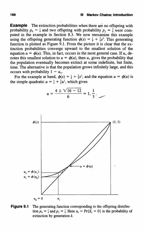
188 III Markov Chains: Introduction
Example The extinction probabilities when there are no offspring withprobability po = 4 and two offspring with probability P2 = 4 were com-puted in the example in Section 8.3. We now reexamine this exampleusing the offspring generating function e(s) = 1 + is2. This generating4 4
function is plotted as Figure 9.1. From the picture it is clear that the ex-tinction probabilities converge upward to the smallest solution of theequation u = ¢(u). This, in fact, occurs in the most general case. If u,. de-notes this smallest solution to u = 4(u), then ux gives the probability thatthe population eventually becomes extinct at some indefinite, but finite,time. The alternative is that the population grows infinitely large, and thisoccurs with probability 1 - ux.
For the example at hand, O(s) = 4 + as2, and the equation u = 4 (u) isthe simple quadratic u = a + 2U2, which gives
4± 1 1
6 1,3
U, 4(u1)
U, 0(uo)
U,
Figure 9.1 The generating function corresponding to the offspring distribu-tion po =4' and p2 = ;. Here u,, = Pr{XA = 0} is the probability ofextinction by generation k.
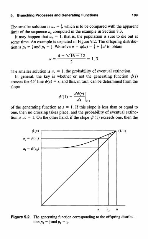
9. Branching Processes and Generating Functions 189
The smaller solution is ux = , which is to be compared with the apparentlimit of the sequence u,, computed in the example in Section 8.3.
It may happen that u,, = 1, that is, the population is sure to die out atsome time. An example is depicted in Figure 9.2: The offspring distribu-tion is po = and p2 = ;. We solve u = (u) _ + ;u2 to obtain
4 ± 16- 12= 1, 3.
2
The smaller solution is ux = 1, the probability of eventual extinction.In general, the key is whether or not the generating function 4(s)
crosses the 45° line ¢(s) = s, and this, in turn, can be determined from theslope
01(1) =do(s)
ds
of the generating function at s = 1. If this slope is less than or equal toone, then no crossing takes place, and the probability of eventual extinc-tion is ux = 1. On the other hand, if the slope 0'(1) exceeds one, then the
0 (u)
U, = O(u,)
ui = 4(uo)
ui u, u
Figure 9.2 The generating function corresponding to the offspring distribu-lion po - and p, = 4

190 III _ Markov Chains: Introduction
equation u = ¢(u) has a smaller solution that is less than one, and extinc-tion is not a certain event.
But the slope 0'(1) of a generating function at s = 1 is the mean E[flof the corresponding distribution. We have thus arrived at the followingimportant conclusion: If the mean offspring size 1, then u,. = 1and extinction is certain. If E[f] > 1, then ux < 1 and the population maygrow unboundedly with positive probability.
The borderline case E[fl = 1 merits some special attention. Here1] = 1 for all n, so the mean population size is constant. Yet the
population is sure to die out eventually! This is a simple example in whichthe mean population size alone does not adequately describe the popula-tion behavior.
9.2. Probability Generating Functions andSums of Independent Random Variables
Let and i be independent nonnegative integer-valued random variableshaving the probability generating functions (p.g.f.s)
O(s) = E[sc] and i/i(s) = E[s"] for IsI < 1.
The probability generating function of the sum + q is simply the prod-uct O(s)4i(s) because
E[s4]E[s''] (because and rl are independent) (9.7)
= 41(s)
The converse is also true. Specifically, if the product of the p.g.f.s oftwo independent random variables is a p.g.f. of a third random variable,then the third random variable equals (in distribution) the sum of the othertwo.
Let .... be independent and identically distributed nonnegativeinteger-valued random variables with p.g.f. 4(s) = E[sf]. Direct inductionof (9.7) implies that the sum , + + ,, has p.g.f.
E[sf +...+',.] = [4(s)]'". (9.8)

9. Branching Processes and Generating Functions 191
We extend this result to determine the p.g f. of a sum of a random numberof independent summands Accordingly, let N be a nonnegative integer-valued random variable, independent of C,, e,, ... , with p.g.f. gN(s) _E[sN], and consider the random sum (see II, Section 3).
X= ,+...+6NLet hx(s) = E[sx] be the p.g.f. of X. We claim that hx(s) takes the simpleform
hx(s) = M[O(s)]. (9.9)
To establish (9.9), consider
hx(s) _ ' Pr{X = k}s"k=0
_ ( Pr{X = kIN = n} Pr{N = n}Is"k=0 n=0 /
k-0 (n=0X D
_7, 1 +6,,=k}Pr{N=n}s"k=0n=0
[because N is independent of ,, 62, ...]
n-0 UO //
X
_ , O(s)" Pr{N = n} [using (9.8)]n=0
= [by the definition of
With the aid of (9.9), the basic branching process equation
X 0,, + ... + :,I, ex" (9.10)
can be expressed equivalently and succinctly by means of generatingfunctions. To this end, let E[sx,] be the p.g.f. of the population sizeX,, at generation n, assuming that X. = 1. Then easily, O0(s) = E[s] = s,and O,(s) = O(s) = E[sc]. To obtain the general expression, we apply (9.9)to (9.10) to yield

192 111 Markov Chains: Introduction
(9.11)
This expression may be iterated in the manner
. 4 [ca(s) } (9.12)
(n + 1) iterations
That is, we obtain the generating function for the population size X,, atgeneration n, given that X0 = 1, by repeated substitution in the probabil-ity generating function of the offspring distribution:
For general initial population sizes X0 = k, the p.g.f. is00
Pr{X =JIX0 = k}s' = (9.13)j=o
exactly that of a sum of k independent lines of descents. From this per-spective, the branching process evolves as the sum of k independentbranching processes, one for each initial parent.
Example Let ¢(s) = q + ps, where 0 < p < 1 and p + q = 1. The as-sociated branching process is a pure death process. In each period eachindividual dies with probability q and survives with probability p. Theiterates in this case are readily determined, e.g., 42(s) = q + p,(q + ps) = 1 - p2 + p'-s, and generally, O,(s) = 1 - p" + p"s. If we fol-low (9.13), the nth generation p.g.f. starting from an initial population sizeof k is [1 - p" + p"s]k.
The probability distribution of the time T to extinction may be deter-mined from the p.g.f. as follows:
Pr{T=nIX(O)=k} =OIXo=k}
[4,(O)]k - [(P"_,(0)]k_ (I - p )k - (I - )k
9.3. Multiple Branching Processes
Population growth processes often involve several life history phases(e.g., juvenile, reproductive adult, senescence) with different viability and

9. Branching Processes and Generating Functions 193
behavioral patterns. We consider a number of examples of branchingprocesses that take account of this characteristic.
For the first example, suppose that a mature individual produces off-spring according to the p.g.f. ¢(s). Consider a population of immature in-dividuals each of which grows to maturity with probability p and then re-produces independently of the status of the remaining members of thepopulation. With probability 1 - p an immature individual will not attainmaturity and thus will leave no descendants. With probability p an indi-vidual will reach maturity and reproduce a number of offspring deter-mined according to the p.g.f. -O(s). Therefore the progeny size distribution(or equivalently the p.g.f.) of a typical immature individual taking accountof both contingencies is
(1 - p) + PO(s). (9.14)
If a census is taken of individuals at the adult (mature) stage, the ag-gregate number of mature individuals contributed by a mature individualwill now have p.g.f.
4(1 - p + ps). (9.15)
(The student should verify this finding.)It is worth emphasis that the p.g.f.s (9.14) and (9.15) have the same
mean p¢'(1) but generally not the same variance, the first being
p[f(l) + 4'(1) - (4'(l))']as compared to
pz4"(1) + p4'(1) - p2(4'(1))2.
Example A second example leading to (9.15), as opposed to (9.14),concerns the different forms of mortality that affect a population. We ap-praise the strength (stability) of a population as the probability of indefi-nite survivorship = 1 - probability of eventual extinction.
In the absence of mortality the offspring number X of a single individ-ual has the p.g.f. 4(s). Assume, consistent with the postulates of a branch-ing process, that all offspring in the population behave independently gov-erned by the same probability laws. Assume also an adult population ofsize X = k. We consider three types of mortality:
(a) Mortality of Individuals Let p be the probability of an offspring sur-viving to reproduce, independently of what happens to others. Thus the

194 III Markov Chains: Introduction
contribution of each litter (family) to the adult population of the next gen-eration has a binomial distribution with parameters (N, p), where N is theprogeny size of the parent with p.g.f. 4(s). The p.g.f. of the adult numberscontributed by a single grandparent is therefore 4(q + ps), q = 1 - p, andfor the population as a whole is '
tp.(s) = [4(q + ps)]'. (9.16)
This type of mortality might reflect predation on adults.
(b) Mortality of Litters Independently of what happens to other litters,each litter survives with probability p and is wiped out with probability q= 1 - p. That is, given an actual litter size , the effective litter size iswith probability p, and 0 with probability q. The p.g.f. of adults in the fol-lowing generation is accordingly
4z(s) _ [q + p4(s)1'. (9.17)
This type of mortality might reflect predation on juveniles or on nests andeggs in the case of birds.
(c) Mortality of Generations An entire generation survives with proba-bility p and is wiped out with probability q. This type of mortality mightrepresent environmental catastrophes (e.g., forest fire, flood). The p.g.f. ofpopulation size in the next generation in this case is
F,(s) = q + p[4(s)]'. (9.18)
All the p.g.f.s (9.16) through (9.18) have the same mean but usually dif-ferent variances.
It is interesting to assess the relative stability of these three models.That is, we need to compare the smallest positive roots of 4,i(s) = s,i = 1, 2, 3, which we will denote by s*, i = 1, 2, 3, respectively.'
We will show by convexity analysis that
4"(s) :5 u2(s) !5; y1,(s)
A function f(x) is convex in x if for every x, and x, and 0 < A < 1, thenf[Ax, + (1 - A)x,] s Af(x,) + (1 - A)f(x,). In particular, the functionQC(s) = G =o pks, for 0 < s < 1 is convex in s, since for each positive in-teger k, [(As,) + (1 - A)s,]' As; + (1 - A)s; for 0 < A, s,, s, < 1. Now,qi,(s) = [4(q + ps)]' < [gca(1) + p4(s)]k = [q + pcb(s)]' = i/i,(s), and thens* < s*. Thus the first model is more stable than the second.

Problems 195
Observe further that due to the convexity of f(x) = x', x > 0, i/r,(s) =[p4(s) + q}' < p[4(s)]k + q X P = /i,(s), and thus s* < s*, implying that2 3
the second model is more stable than the third model. In conjunction weget the ordering s* < s* < s*.
Exercises
9.1. Suppose that the offspring distribution is Poisson with meanA = 1.1. Compute the extinction probabilities u = Pr (X,, = 01X0 = I) forn = 0, 1, . . . , 5. What is ux, the probability of ultimate extinction?
9.2 Determine the probability generating function for the offspring dis-tribution in which an individual either dies, with probability po, or is re-placed by two progeny, with probability P21 where po + P2 = 1.
9.3. Determine the probability generating function corresponding to theoffspring distribution in which each individual produces 0 or N direct de-scendants, with probabilities p and q, respectively.
9.4. Let ¢(s) be the generating function of an offspring random variable6. Let Z be a random variable whose distribution is that of , but condi-tional on > 0. That is,
Pr{Z=k} fork= 1,2.....Express the generating function for Z in terms of 4.
Problems
9.1. One-fourth of the married couples in a far-off society have no chil-dren at all. The other three-fourths of families have exactly three children,each child equally likely to be a boy or a girl. What is the probability thatthe male line of descent of a particular husband will eventually die out?
9.2. One-fourth of the married couples in a far-off society have exactlythree children. The other three-fourths of families continue to have chil-dren until the first boy and then cease childbearing. Assume that eachchild is equally likely to be a boy or girl. What is the probability that themale line of descent of a particular husband will eventually die out?

196 III Markov Chains: Introduction
9.3. Consider a large region consisting of many subareas. Each subareacontains a branching process that is characterized by a Poisson distribu-tion with parameter A. Assume, furthermore, that the value of A varieswith the subarea, and its distribution over the whole region is that of agamma distribution. Formally, suppose that the offspring distribution isgiven by
e-ASR7r(kj1k)
=k!
for k = 0, 1,\\.,
where A itself is a random variable having the density function
6«A«ie0Afor A > 0,f(A) F(a)F(a)
where 6 and a are positive constants. Determine the marginal offspringdistribution pA = f ir(kl A)f(A) dA.
Hint: Refer to the last example of II, Section 4.
9.4. Let 4(s) = 1 - p(1 - s),', where p and /3 are constants with 0 < p,/3 < 1. Prove that O(s) is a probability generating function and that itsiterates are
0,,(s) = 1 -pl+a+...+1.,-I(1 - s)a' for n = 1,2,....
9.5. At time 0, a blood culture starts with one red cell. At the end of oneminute, the red cell dies and is replaced by one of the following combi-nations with the probabilities as indicated:
2 red cells1 red, 1 white
2 white
Each red cell lives for one minute and gives birth to offspring in the sameway as the parent cell. Each white cell lives for one minute and dies with-out reproducing. Assume that individual cells behave independently.
(a) At time n + 1 minutes after the culture begins, what is the proba-bility that no white cells have yet appeared?
(b) What is the probability that the entire culture eventually dies outentirely?

Problems 197
9.6. Let ¢(s) = as- + bs + c, where a, b, c are positive and 4(l) = 1.Assume that the probability of extinction is u., where 0 < u,, < 1. Provethat u = cla.
9.7. Families in a certain society choose the number of children thatthey will have according to the following rule: If the first child is a girl,they have exactly one more child. If the first child is a boy, they continueto have children until the first girl and then cease childbearing. Let 6 bethe number of male children in a particular family. What is the generatingfunction of V. Determine the mean of 6 directly and by differentiating thegenerating function.
9.8. Consider a branching process whose offspring follow the geomet-ric distribution pk = (1 - c)ck for k = 0, 1, ... , where 0 < c < 1. Deter-mine the probability of eventual extinction.
9.9. One-fourth of the married couples in a distant society have no chil-dren at all. The other three-fourths of families continue to have childrenuntil the first girl and then cease childbearing. Assume that each child isequally likely to be a boy or girl.
(a) For k = 0, 1, 2, . . . , what is the probability that a particular hus-band will have k male offspring?
(b) What is the probability that the husband's male line of descent willcease to exist by the 5th generation?
9.10. Suppose that in a branching process the number of offspring of aninitial particle has a distribution whose generating function is f(s). Eachmember of the first generation has a number of offspring whose distribu-tion has generating function g(s). The next generation has generatingfunction f, the next has g, and the distributions continue to alternate in thisway from generation to generation.
(a) Determine the extinction probability of the process in terms of f(s)and g(s).
(b) Determine the mean population size at generation n.(c) Would any of these quantities change if the process started with the
g(s) process and then continued to alternate?


Chapter IVThe Long Run Behavior of
Markov Chains
1. Regular Transition Probability Matrices
Suppose that a transition probability matrix P =j on a finite number ofstates labeled 0, 1, . . . , N has the property that when raised to somepower k, the matrix Pk has all of its elements strictly positive. Such a tran-sition probability matrix, or the corresponding Markov chain, is calledregular. The most important fact concerning a regular Markov chain is theexistence of a limiting probability distribution it = (iro, 1r,, . . . , TrN),
where i r, > 0 for j = 0, 1, ... , N and I; 7rj = 1, and this distribution isindependent of the initial state. Formally, for a regular transition proba-bility matrix P = P, we have the convergence
limP;;'= Tr;>0 forj=0, 1,...,N,/1-)r.
or, in terms of the Markov chain
lim Pr{X = jjX0 = i } = 7 r ; > 0 for j = 0, 1, ... , N.I)--
This convergence means that, in the long run (n -4 co), the probabilityof finding the Markov chain in state j is approximately Tr; no matter inwhich state the chain began at time 0.

200 IV The Long Run Behavior of Markov Chains
Example The Markov chain whose transition probability matrix is
0 1
P _0I 1-a a1 b 1-b.
is regular when 0 < a, b < 1, and in this case the limiting distribution is1r = (b/(a + b), a/(a + b)). To give a numerical example, we will supposethat
0.33 0.67P
0.75 0.25
The first several powers of P are given here:
P'0.6114_ II
0.43500.38860.5650
P3 =0.49320.5673
0.506811
0.4327 '
P4= 0.5428 0.4572 P5 = 0.5220 0.47800.5117 0.4883 0.5350 0.4560 '
p6 = 0.5307 0.4693I P
0.5271 0.47290.5253 0.4747 ' 0.5294 0.4706
By n = 7, the entries agree row-to-row to two decimal places. The limit-ing probabilities are b/(a + b) = 0.5282 and a/(a + b) = 0.4718.
Example Sociologists often assume that the social classes of succes-sive generations in a family can be regarded as a Markov chain. Thus, theoccupation of a son is assumed to depend only on his father's occupationand not on his grandfather's. Suppose that such a model is appropriate andthat the transition probability matrix is given by
Son's ClassLower Middle Upper
'Lower 40 0 500 100Father s
ClMiddle
. .
05 0 700
.
0 25ass Upper..
0.05 0.50
.
0.45

1. Regular Transition Probability Matrices 201
For such a population, what fraction of people are middle class in the longrun?
For the time being, we will answer the question by computing suffi-ciently high powers of P' A better method for determining the limitingdistribution will be presented later in this section.
We compute
0.1900 0.6000 0.2100
P2=PxP= 0.0675 0.6400 0.2925
0.0675 0.6000 0.3325
0.0908 0.6240 0.2852
P2=PxP= 0.0758 0.6256 0.2986
0.0758 0.6240 0.3002
0.0772 0.6250 0.2978
P8= P4XP4= 0.0769 0.6250 0.2981
0.0769 0.6250 0.2981
Note that we have not computed P" for consecutive values of n but havespeeded up the calculations by evaluating the successive squares P2,P4, P8.
In the long run, approximately 62.5 percent of the population are mid-dle class under the assumptions of the model.
Computing the limiting distribution by raising the transition probabilitymatrix to a high power suffers from being inexact, since n = 00 is neverattained, and it also requires more computational effort than is necessary.Theorem 1.1 provides an alternative computational approach by assertingthat the limiting distribution is the unique solution to a set of linear equa-tions. For this social class example, the exact limiting distribution, com-puted using the method of Theorem 1.1, is aro = ,=; = 0.0769, ir, = s =0.6250, andir2=;O',=0.2981.
If a transition probability matrix P on N states is regular, thenPNZ
willhave no zero elements. Conversely, if PN' is not strictly positive, then theMarkov chain is not regular. Furthermore, once it happens that Pk has nozero entries, then every higher power P'`+", n = 1, 2, . . . , will have no zeroentries. Thus it suffices to check the successive squares P, P2, P4, P8. ... .

202 IV The Long Run Behavior of Markov Chains7Finally, to determine whether or not the square of a transition probabilitymatrix has only strictly positive entries, it is not necessary to perform theactual multiplication, but only to record whether or not the product isnonzero.
Example Consider the transition probability matrix
0.9 0.1 0 0 0 0 0
0.9 0 0.1 0 0 0 0
0.9 0 0 0.1 0 0 0
P= 0.9 0 0 0 0.1 0 0
0.9 0 0 0 0 0.1 0
0.9 0 0 0 0 0 0.1
0.9 0 0 0 0 0 0.1
We recognize this as a success runs Markov chain. We record the nonzeroentries as + and write P X P in the form
++ 0 0 0 0 0
+ 0+ 0 0 0 0
+ 0 0+ 0 0 0
PxP= + 0 0 0 + 0 0
+ 0 0 0 0 + 0
+ 0 0 0 0 0++ 0 0 0 0 0 +
++ 0 0 0 0 0
+ 0+ 0 0 0 0
+ 0 0+ 0 0 0
x + 0 0 0 + 0 0
+ 0 0 0 0 + 0
+ 0 0 0 0 0++ 0 0 0 0 0+

1. Regular Transition Probability Matrices 203
P4 =
P8 =
+ + + 0 0 0 0
+ + 0 + 0 0 0
+ + 0 0 + 0 0
+ + 0 0 0 + 0
+ + 0 0 0 0 +
+ + 0 0 0 0 +
+ + 0 0 0 0 +
+ + + + + 0 0
+ + + + 0 + 0
+ + + + 0 0 +
+ + + + 0 0 +
+ + + + 0 0 +
+ + + + 0 0 +
+ + + + 0 0 +
= P2
,
We see that P8 has all strictly positive entries, and therefore P is regular.The limiting distribution for a similar matrix is computed in Section 2.2.
Every transition probability matrix on the states 0, 1, . . . , N that satis-fies the following two conditions is regular:
1. For every pair of states i, j there is a path k ... , kr for which Pk,P,k>...P;>0.
2. There is at least one state i for which P; > 0.

204 IV The Long Run Behavior of Markov ChainsV
Theorem 1.1 Let P be a regular transition probability matrix on thestates 0, 1, . . . , N. Then the limiting distribution err = (iro, Tr ... ire,) isthe unique nonnegative solution of the equations
k=0
N
1kk=0
1TkPkj,
= 1. (1.3)
Proof Because the Markov chain is regular, we have a limiting distrib-ution, lim,,. P;' = .7r j, for which I 0 irk = 1. Write P" as the matrix prod-j k=
uct P"-' P in the form
ifk=0
P1"-"P = 0, . . N,k kj j ,
and now let n - oo. Then P;;' -* irj, while P,k"-" -4 4rk, and (1.4) passesinto Trj = Jko ITkPkj as claimed.
It remains to show that the solution is unique. Suppose that x0, x,, ... ,x1 solves
andN
(1.6)
k=0
We wish to show that xj = if,, the limiting probability. Begin by multi-plying (1.5) on the right by P, and then sum over j to get
N N N NP,=Y_ 7, xkPjI,_
j=0 j=0 k=0 k=0
But by (1.5) we have x, _ J o xjPj,, whence (1.7) becomesN
X, _ p(2)I k(
j=0,1,...,N, (1.2)
for 1= 0, ...,N.k=0
Repeating this argument n times we deduce thatN
x,xkP(") fort=0,...,N,k=0
N
xj=7, xkPkj forj=0,...,N (1.5)k=0
(1.7)

1. Regular Transition Probability Matrices 205
and then passing to the limit in n and using that P(k'; - 7r, we see thatN
XI ZXk7r 1=0,...,N.k=0
But by (1.6) we have lk Xk = 1, whence x, = 7r, as claimed.
Example For the social class matrix
0 1 2
0 0.40 0.50 0.10
P=1 0.05 0.70 0.25
2 0.05 0.50 0.45
the equations determining the limiting distribution ('7ro, 7x,, 7r2) are
0.40770 + 0.057x, + 0.057x2 = 7ro, (1.8)
0.507x0 + 0.707r, + 0.507x2 = 7r,, (1.9)
0.107x0 + 0.257r, + 0.457x2 = 7x2, (1.10)
1r0+ 7r,+ 7x2=1. (1.11)
One of the equations (1.8), (1.9), and (1.10) is redundant, because of thelinear constraint Ik Pk = 1. We arbitrarily strike out (1.10) and simplifythe remaining equations to get
-607ra+57x,+57r,=0, (1.12)
57ro - 37r, + 57x, = 0, (1.13)
7ro + 7r, + 7x2 = 1. (1.14)
We eliminate 7x2 by subtracting (1.12) from (1.13) and five times (1.14) toreduce the system to
657ro-87x,=0,
657x0 = 5.
Then Ira = bs = ,=,, 7r, _ $, and then 7r, = 1 - 7ro - 7r, _ ;0, as given earlier.
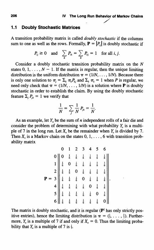
206 IV The Long Run Behavior of Markov ChainsV
1.1 Doubly Stochastic Matrices
A transition probability matrix is called doubly stochastic if the columnssum to one as well as the rows. Formally, P = IP;I is doubly stochastic if
P; 0 and 7, Pk =k k
Pk1 = 1 for all i, j.
Consider a doubly stochastic transition probability matrix on the Nstates 0, 1, . . . , N - 1. If the matrix is regular, then the unique limitingdistribution is the uniform distribution ?r = (1/N, ... , 1/N). Because thereis only one solution to 7r; = 1k irkPk1 and Ik 7rk = 1 when P is regular, weneed only check that 'rr = (1/N, ... , 1/N) is a solution where P is doublystochastic in order to establish the claim. By using the doubly stochasticfeature I; Pi, = 1 we verify that
As an example, let Y,, be the sum of n independent rolls of a fair die andconsider the problem of determining with what probability Y is a multi-ple of 7 in the long run. Let X,, be the remainder when Y is divided by 7.Then X,, is a Markov chain on the states 0, 1, ... , 6 with transition prob-ability matrix
2 3 4
1 I I
6 6 6
1 1
6 6 6
0 1
6 6
06 6
I I
The matrix is doubly stochastic, and it is regular (P2 has only strictly pos-itive entries), hence the limiting distribution is 'rr = (1, . . . , 1). Further-7 7
more, Y is a multiple of 7 if and only if X,, = 0. Thus the limiting proba-bility that Y is a multiple of 7 is ;.

1. Regular Transition Probability Matrices 207
1.2 Interpretation of the Limiting Distribution
Given a regular transition matrix P for a Markov process {X,,} on theN + 1 states 0, 1, . . . , N, we solve the linear equations
N
and
for i = 0, 1, . . . , NTTkPkrk=O
7ro+ IF, + + 7r,,,= 1.
The primary interpretation of the solution (7ro, ... , 7r,,,) is as the limitingdistribution
7r; = lim P;;) = lim Pr{X = jl Xo = i }.
In words, after the process has been in operation for a long duration, theprobability of finding the process in state j is 7r;, irrespective of the start-ing state.
There is a second interpretation of the limiting distribution 'rr =(7ro, 7r . . . , 7rN) that plays a major role in many models. We claim that7r; also gives the long run mean fraction of time that the process is instate j. Thus if each visit to state j incurs a "cost" of c;, then the long runmean cost per unit time associated with this Markov chain is
Long run mean cost per unit time =N
i=o
To verify this interpretation, recall that if a sequence a,,, a,, . . . of realnumbers converges to a limit a, then the averages of these numbers alsoconverge in the manner
1 ,,,-Ilim - 7 ak = a.11- ' m k=O
We apply this result to the convergence P;' = 7r; to conclude that
I ,,,-Prk> _lim - 7 ;; 7r1.

208 IV The Long Run Behavior of Markov Chains7Now, (1/m) Y,k o is exactly the mean fraction of time during steps0, 1, ... , m - 1 that the process spends in state j. Indeed, the actual (ran-dom) fraction of time in state j is
1 in-1-7, 1{Xk=j},m k=0
where
11Xk= }=1 ifXk =j,
fo if X *f.Therefore the mean fraction of visits is obtained by taking expected val-ues according to
f1 in-1 1m-iEL->2 1{Xk=j}IXo=ij=- E[1{Xk=j}IXo=i]
M k=0 m k=0
m-17 Pr(Xk = AXo = I}
m k=0
1 in-1p;k1.
m k=0
Because lim,,. P;'' = n , the long run mean fraction of time that theprocess spends in state j is
r 1m-1 1 1m-1lim El - 11Xk = j}IXo = iJ = 1im - I P;;' = 7rj,
m k=0 m k=0
independent of the starting state i.
Exercises
1.1. A Markov chain X0, X X,, . . . has the transition probability matrix
0 1 2
0 0.7 0. 2 0.1
P=1 0 0. 6 0.4
2 0.5 0 0.5
Determine the limiting distribution.
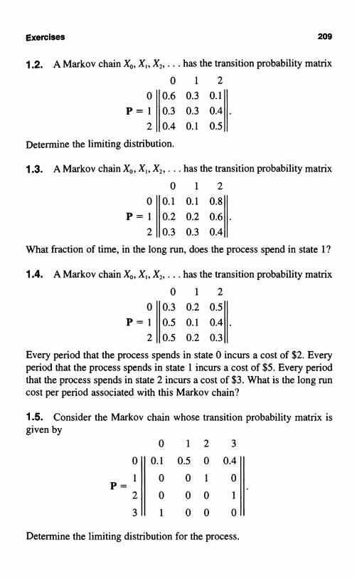
Exercises 209
1.2. A Markov chain X0, X X2.... has the transition probability matrix
0 1 2
0 0.6 0.3 0.1
P=1 0.3 0.3 0.4
2 0.4 0.1 0.5
Determine the limiting distribution.
1.3. A Markov chain X0, X,, X2, ... has the transition probability matrix
0 1 2
0 0.1 0.1 0.8
P = 1 0.2 0.2 0.6
2 0.3 0.3 0.4
What fraction of time, in the long run, does the process spend in state I?
1.4. A Markov chain X0, X X,.... has the transition probability matrix
0 1 2
0 0.3 0.2 0.5
P = 1 0.5 0.1 0.4
2 0.5 0.2 0.3
Every period that the process spends in state 0 incurs a cost of $2. Everyperiod that the process spends in state 1 incurs a cost of $5. Every periodthat the process spends in state 2 incurs a cost of $3. What is the long runcost per period associated with this Markov chain?
1.5. Consider the Markov chain whose transition probability matrix isgiven by
0 1 2 3
0 0.1 0.5 0 0.4
1 0 0 1 0P
2 0 0 0 1
3 1 0 0 0
Determine the limiting distribution for the process.

210 IV The Long Run Behavior of Markov Chains
1.6. Compute the limiting distribution for the transition probabilitymatrix
0 1 2
0 ' ' 02 2
1 1 1P=13 3 3
2 6 2 3
1.7. A Markov chain on the states 0, 1, 2, 3 has the transition probabil-ity matrix
0 1 2 3
0 0.1 0.2 0.3 0.4
1 0 0 3 30 40P=
. . .
2 0 0 0.6 0.4
3 1 0 0 0
Determine the corresponding limiting distribution.
1.8. Suppose that the social classes of successive generations in a fam-ily follow a Markov chain with transition probability matrix given by
Son's Class
'Lower
Lower0 7
Middle
0 2
Upper10Father s
ClMiddle
.
0 2
.
0 6
.
0 2ass Upper.
0.1
.
0.4
.
0.5
What fraction of families are upper class in the long run?
1.9. Determine the limiting distribution for the Markov chain whosetransition probability matrix is
2
0
6
3
1.10. A bus in a mass transit system is operating on a continuous routewith intermediate stops. The arrival of the bus at a stop is classified intoone of three states, namely

problems 211
1. Early arrival;2. On-time arrival;3. Late arrival.
Suppose that the successive states form a Markov chain with transitionprobability matrix
1 2 3
1 0.5 0.4 0.1
P=2 0.2 0.5 0.3
3 0.1 0.2 0.7
Over a long period of time, what fraction of stops can be expected to be late?
Problems
1.1. Five balls are distributed between two urns, labeled A and B. Eachperiod, an urn is selected at random, and if it is not empty, a ball from thaturn is removed and placed into the other urn. In the long run, what frac-tion of time is urn A empty?
1.2. Five balls are distributed between two urns, labeled A and B. Eachperiod, one of the five balls is selected at random, and whichever urn it'sin, it is moved to the other urn. In the long run, what fraction of time isurn A empty?
1.3. A Markov chain has the transition probability matrix
0 1 2 3 4 5
0 C11 a, a3 a4 a5 a6
1 1 0 0 0 0 0
2 0 1 0 0 0 0P=
3 0 0 1 0 0 0
4 0 0 0 1 0 0
5 0 0 0 0 1 0
where a; ? 0, i = 1, ... , 6, and a, + + a6 = 1. Determine the lim-iting probability of being in state 0.

212 IV The Long Run Behavior of Markov Chains
1.4. A finite state regular Markov chain has transition probability matrixP = NP;j and limiting distribution IT = PIT;j. In the long run, what fractionof the transitions are from a presribed state k to a prescribed state m?
1.5. The four towns A, B, C, and D are connected by railroad lines asshown in the following diagram:
Figure 1.1 A graph whose nodes represent towns and whose arcs representrailroad lines.
Each day, in whichever town it is in, a train chooses one of the lines outof that town at random and traverses it to the next town, where the processrepeats the next day. In the long run, what is the probability of finding thetrain in town D?
1.6. Determine the following limits in terms of the transition probabil-ity matrix P = II1 J0 and limiting distribution 'rr = I7r 11 of a finite state reg-ular Markov chain
(a) jjX0 = i}.(b) Pr{X = k, jXo = i}.(c) lim,,. k, X, = jjX0 = i}.
1.7. Determine the limiting distribution for the Markov chain whosetransition probability matrix is
0 1 2 3
0 2 0 0 _
1 1 0 0 0P=
2 0 ' ' '2 3 6
3 0 0 1 0

Problems 213
1.8.
0 1 2 3 4
0 0 '2
i
2 0 0
1 0 0 0
P=2 3 3 0 0
3 0 0 2 0 2
4 0 0 0
is regular and compute the limiting distribution.
1.9. Determine the long run, or limiting, distribution for the Markovchain whose transition probability matrix is
0 1 2 3
0 0 1 0
0 0 0 1
4 4 4 4
0 0 ' '2 2
1.10. Consider a Markov chain with transition probability matrix
P=
Po A P2 PN
PN Po P i PN-1
PN-I PN Po PN-2
PA P2 P3 " ' Po
where 0 < po < 1 and po + p, + + PN = 1. Determine the limiting dis-tribution.
Show that the transition probability matrix
1.11. Suppose that a production process changes state according to aMarkov process whose transition probability matrix is given by

214 IV The Long-Run Behavior of Markov Chains
0 1 2 3
0.3 0.5 0 0.2
0.5 0.2 0.2 0.1P
2 0.2 0.3 0.4 0.1
3 0.1 0.2 0.4 0.3
It is known that ?r, = 3;-9 = 0.3140 and ar, = ;;9 = 0.2137.
(a) Determine the limiting probabilities .7ro and it .
(b) Suppose that states 0 and 1 are "In-Control" while states 2 and 3 aredeemed "Out-of-Control." In the long run, what fraction of time isthe process Out-of-Control?
(c) In the long run, what fraction of transitions are from an In-Controlstate to an Out-of-Control state?
1.12 Let P be the transition probability matrix of a finite state regularMarkov chain, and let n be the matrix whose rows are the stationary dis-tribution ir. Define Q = P - 11.
(a) Show that P" = H + Q".(b) When
P=0 ' '2 2
obtain an explicit expression for Q' and then for P".
1.13. A Markov chain has the transition probability matrix
0 1 2
0 0.4 0.4 0.2
P=1 0.6 0.2 0.2
2 0.4 0.2 0.4

2. Examples 215
After a long period of time, you observe the chain and see that it is instate 1. What is the conditional probability that the previous state was state2? That is, find
lim 21X = 1}.
2. Examples
Markov chains arising in meteorology, reliability, statistical quality con-trol, and management science are presented next, and the long run behav-ior of each Markov chain is developed and interpreted in terms of the phe-nomenon under study.
2.1. Including History in the State Description
Often a phenomenon that is not naturally a Markov process can be mod-eled as a Markov process by including part of the past history in the statedescription. To illustrate this technique, we suppose that the weather onany day depends on the weather conditions for the previous two days. Tobe exact, we suppose that if it was sunny today and yesterday, then it willbe sunny tomorrow with probability 0.8; if it was sunny today but cloudyyesterday, then it will be sunny tomorrow with probability 0.6; if it wascloudy today but sunny yesterday, then it will be sunny tomorrow withprobability 0.4; if it was cloudy for the last two days, then it will be sunnytomorrow with probability 0.1.
Such a model can be transformed into a Markov chain, provided we saythat the state at any time is determined by the weather conditions duringboth that day and the previous day. We say the process is in
State (S, S) if it was sunny both today and yesterday,State (S, C) if it was sunny yesterday but cloudy today,State (C, S) if it was cloudy yesterday but sunny today,State (C, C) if it was cloudy both today and yesterday.
Then the transition probability matrix is

216 IV The Long Run Behavior of Markov Chains
Today's State(S, S) (S, C) (Cl S) (C, C)
(S,S) 0.8 0.2
Yesterday's (S, C) 0.4 0.6
State (C, S) 0.6 0.4
(C, C) 0.1 0.9
The equations determining the limiting distribution are
0.81ro + 0.67x, = 7ro,
0.27ro + 0.47r, = 7r
0.47x, + 0.17x, = 7r,,
0.67r, 0.9'7, = 7"
Ira + 7r, + 7r, + 7r3 = 1.
Again, one of the top four equations is redundant. Striking out the firstequation and solving the remaining four equations gives 7ro = ;,, 7r,7r,=,, and 7r,=.
We recover the fraction of days, in the long run, on which it is sunny bysumming the appropriate terms in the limiting distribution. It can be sunnytoday in conjunction with either being sunny or cloudy tomorrow. There-fore, the long run fraction of days in which it is sunny is 7ro + 7r, =7r(S, S) + 7r(S, C) Formally, Pr{X = S} = lim,, ,. [Pr{X = S,
=S} =C}] = ITO+7r,.
2.2. Reliability and Redundancy
An airline reservation system has two computers, only one of which is inoperation at any given time. A computer may break down on any givenday with probability p. There is a single repair facility that takes 2 days torestore a computer to normal. The facilities are such that only one com-puter at a time can be dealt with. Form a Markov chain by taking as statesthe pairs (x, y) where x is the number of machines in operating conditionat the end of a day and y is 1 if a day's labor has been expended on a ma-chine not yet repaired and 0 otherwise. The transition matrix is

2. Examples
To State
From State1
(2, 0)
P=(1,0)
(1, 1)
(0, 1)
-+ (2, 0) (1, 0) (1, 1) (0, 1)
q p 0 0
0 0 q p
q p 0 0
0 1 0 0
217
wherep + q = I.We are interested in the long run probability that both machines are in-
operative. Let (4ro, ir,, 7r,, ir3) be the limiting distribution of the Markovchain. Then the long run probability that neither computer is operating is1r3, and the availability, the probability that at least one computer is oper-ating,is1-7r3=fro+7r,+,TZ.
The equations for the limiting distributions are
giro + qir, _ iro,
PIro +pIr,+Ira=?r,,
qIT, =ITz,
and
The solution is
= I3PITS
7ro+1r,+9r,+Ir3=1.
q2 qp110 p2' ir, 1+p-
P P2
Ir, _ +P 2' 7r3 = +p 2.
l l
The availability is R, = 1 - 7T3 = 1/(1 + p2).In order to increase the system availability, it is proposed to add a du-
plicate repair facility so that both computers can be repaired simultane-ously. The corresponding transition matrix is now

218 IV The Long Ru n Behavior o f Markov Chains
To State- (2, 0) (1, 0) (1, 1) (0, 1)
From State1
(2, 0) q p 0 0
P_(1,0) 0 0 . q p
(1, 1) q p 0 0
(0, 1) 0 0 1 0
and the limiting distribution is
= q PITO , ,,1 +p+p - l +p+p -
P 73 _P_
*1 +p+p2 1+p+p2
Thus availability has increased to R, = 1 - TT, = (1 + p)/(1 + p + p2).
2.3. A Continuous Sampling Plan
Consider a production line where each item has probability p of beingdefective. Assume that the condition of a particular item (defective ornondefective) does not depend on the conditions of other items. The fol-lowing sampling plan is used.
Initially every item is sampled as it is produced; this procedure contin-ues until i consecutive nondefective items are found. Then the samplingplan calls for sampling only one out of every r items at random until a de-fective one is found. When this happens the plan calls for reverting to 100percent sampling until i consecutive nondefective items are found. Theprocess continues in the same way.
State Ek (k = 0, 1, . . . , i - 1) denotes that k consecutive nondefectiveitems have been found in the 100 percent sampling portion of the plan,while state E; denotes that the plan is in the second stage (sampling oneout of r). Time m is considered to follow the mth item, whether sampledor not. Then the sequence of states is a Markov chain with

2. Examples 219
pi, = Pr{in state Ek after m + 1 itemslin state E; after m items}
p fork= 0,0-j<i,1-p for k=j+1<i,P fork=O,j=i,r
1- p- fork=j=i,r
0 otherwise.
Let ark be the limiting probability that the system is in state Ek fork = 0, 1, . . . , i. The equations determining these limiting probabilities are
(0) PITo+ par,+ + (plr) ar; = ITo,
(1) (1 - p)'ro = IT,,
(2) (1 - P)irI
(i) (1 - p)'T, + (1 - plr)ar, = 'Ti
together with
(*) 1T0+IT1+...+ar=1.
From equations (1) through (i) we deduce that ark = (1 - park-,, so thatark = (1 - p)karo for k = 0, . . . , i - 1, while equation (i) yields ar; =(r1p)(1 - p)ar;_, or ar, _ (rlp)(1 - p)'aro. Having determined ark in termsof aro for k = 0, . . . , i, we place these values in (*) to obtain
{[1 + ... + (1 - p)'-,} +p (1 - p)'}iro = 1.
The geometric series simplifies, and after elementary algebra the solutionis
p1To = 1 + (r - 1)(1 - p);,

220
whence
while
IV The Long Run Behavior of Markov Chains
P(1 - P)kTrk 1 + (r - 1)(1 - p)' fork=0,...,i-1,
r(1 - p)'ir' 1+(r-1)(1-p)"
Let AFI (Average Fraction Inspected) denote the long run fraction ofitems that are inspected. Since each item is inspected while in statesE0, ... , E;_, but only one out of r is inspected in state E;, we have
AFI = (7ro + + iri-,) + (1/r)ir,
_ (1 - ?r;) + (1/r)ir,
1
1 + (r - 1)(1 - p)'
Let us assume that each item found to be defective is replaced by anitem known to be good. The average outgoing quality (AOQ) is defined tobe the fraction of defectives in the output of such an inspection scheme.The average fraction not inspected is
1 - AFI=(r - 1)(1 - p)'
1 + (r- 1)(1 -p)"
and of these on the average p are defective. Hence
AOQ = (r - 1)(1 P)P1 + (r - 1)(1 - p)'
This average outgoing quality is zero if p = 0 orp = 1, and rises to a max-imum at some intermediate value, as shown in Figure 2.1. The maximumAOQ is called the average outgoing quality limit (AOQL), and it has beendetermined numerically and tabulated as a function of i and r.
This quality control scheme guarantees an output quality better than theAOQL regardless of the input fraction defective, as shown in Figure 2.2.

2. Examples 221
a0
0 p
AOQL
1
Figure 2.1 The average outgoing quality (AOQ) as a function of the inputquality level p
INPUT
Arbitrary Quality
p
CONTINUOUSSAMPLING
INSPECTION
OUTPUT
Guaranteed QualityAOQL
Figure 2.2 Black-box picture of a continuous inspection scheme as a methodof guaranteeing outgoing quality
2.4. Age Replacement Policies
A component of a computer has an active life, measured in discrete units,that is a random variable T, where Pr[T = k] = ak for k = 1, 2, .... Sup-pose one starts with a fresh component, and each component is replacedby a new component upon failure. Let X,, be the age of the component inservice at time n. Then is a success runs Markov chain. (See III, Sec-tion 5.4.)
In an attempt to replace components before they fail in service, an agereplacement policy is instituted. This policy calls for replacing the com-ponent upon its failure or upon its reaching age N, whichever occurs first.Under this age replacement policy, the Markov chain has the transi-tion probability matrix

222 IV The Long Run Behavior of Markov Chains
0
1
P= 2
N-1
where
0 1 2 3 N- 1Po 1 -PO 0 0 0
A 0 1 - p, 0 0
P2 0 0 1 - P2 ... 0
1 0 0 0 0
Pkak+l fork=0,1,...,N-2.
ak+I + ak+2 +
State 0 corresponds to a new component, and therefore the limitingprobability 7ro corresponds to the long run probability of replacement dur-ing any single time unit, or the long run replacement per unit time. Someof these replacements are planned or age replacements, and some corre-spond to failures in service. A planned replacement occurs in each periodfor which X,, = N - 1, and therefore the long run planned replacementsper unit time is the limiting probability 7TN-,. The difference 7ro - 7TN-, isthe long run rate of failures in service. The equations for the limiting dis-tribution 7r = (7ro, 7T,, ... , 7TN-,) are
P0ir0 + P1n1 + + PN-2ITN-2 + irN-1 = TAO,
(1 - P0)iro = IT1,
(1 - PI)Tr, = 72,
(1 PN-2)ITN-2 = IrN-1,
7ro + 7r, + .. .
Solving in terms of 7ro, we obtain
ITo = 1T0,
I, = (1 - Po) 7T0,
IT2 = (1 - P1)7r1 = (1 - PI)(1 - PO)ITo,
+ 7TN-I = 1.
1Tk = (1 Pk-1)lTk-1 = (1 Pk-l)(1 Pk-2) ... (1 - PO)n0,
'TN-1 = (1 PN-2)7rN-2 = (1 PN-2)(l PN-3) ... (1 - P0)ir0,

2. Examples 223
and since iro + 7T, + + 7rv-, = 1, we have
1 = [1 +(I -Po)+(I -Po)(I -Pi)+...
+ (1 - NO - Pi) ... (I - PN_2)]moo,
or
I
1 + (1 - Po) + (I - Pp)(I P) + ... + (I - Po)(1 - Pi) ... (I - PN-2)
If A; = a; + a;+, + for j = 1, 2, ... , where A, = 1, then Pk = ak+,/Ak+,and 1 - Pk = Ak+,/Ak+,, which simplifies the expression for 7rp to
1ITo=A,+A,+...+Av'
and then
Tr =A 7r =A,
v-1 ,v A, + A, + ... + A,*
In practice, one determines the cost C of a replacement and the addi-tional cost K that is incurred when a failure in service occurs. Then thelong run total cost per unit time is Ciro + K(Iro - and the replace-ment age N is chosen so as to minimize this total cost per unit time.
Observe that
= A, + A, + + ANITO
N-I
Pr{T ? j} _ Pr{T > k}k=0
Pr{min{T, N} > k} = E[min(T, N}].
J=1X
k=0
In words, the reciprocal of the mean time between replacementsE[min{T, N}] yields the long run replacements per unit time iro. This re-lation will be further explored in the chapter on renewal processes.
2.5. Optimal Replacement Rules
A common industrial activity is the periodic inspection of some system aspart of a procedure for keeping it operative. After each inspection, a deci-sion must be made whether or not to alter the system at that time. If the

224 IV The Long Run Behav r of Markov Chains
inspection procedure and the ways of modifying the system are fixed, animportant problem is that of determining, according to some cost criterion,the optimal rule for making the appropriate decision. Here we consider thecase in which the only possible act is to replace the system with a new one.
Suppose that the system is inspected at equally spaced points in timeand that after each inspection it is classified into one of the L + 1 possi-ble states 0, 1, . . . , L. A system is in state 0 if and only if it is new and isin state L if and only if it is inoperative. Let the inspection times be n =0, 1, . . . , and let X,, denote the observed state of the system at time n. Inthe absence of replacement we assume that is a Markov chain withtransition probabilities p;; = jl X,, = i} for all i, j, and n.
It is possible to replace the system at any time before failure. The mo-tivation for doing so may be to avoid the possible consequences of furtherdeterioration or of failure of the system. A replacement rule, denoted byR, is a specification of those states at which the system will be replaced.Replacement takes place at the next inspection time. A replacement rule Rmodifies the behavior of the system and results in a modified Markovchain n = 0, 1, ... }. The corresponding modified transition prob-abilities p;;(R) are given by
p,(R) = p;; if the system is not replaced at state i,
p,o(R) = 1,
and
p;; (R) = 0, j 0 0 if the system is replaced at state i.
It is assumed that each time the equipment is replaced, a replacementcost of K units is incurred. Further it is assumed that each unit of time thesystem is in state j incurs an operating cost of a;. Note that a. may be in-terpreted as failure (inoperative) cost. This interpretation leads to the oneperiod cost function c;(R) given for i = 0, . . . , L by
c, (R) =a, if p,o(R) = 0,K + a; if p;o(R) = 1.
We are interested in replacement rules that minimize the expected longrun time average cost. This cost is given by the expected cost under thelimiting distribution for the Markov chain Denoting this averagecost by 4(R), we have

2. Examples 225
(k(R) _ , 7r;(R)c;(R),i=O
where ir;(R) = lim,,., i}. The limiting distribution 7r;(R) is de-termined by the equations
L
iT;(R) _ irk(R)pk;(R), i = 0, ... , L,k=O
and
lTo(R) + ir(R) + ... + lrL(R) = 1.
We define a control limit rule to be a replacement rule of the form
"Replace the system if and only if X,, ? k,"
where k, called the control limit, is some fixed state between 0 and L. Welet Rk denote the control limit rule with control limit equal to k. Then Ro isthe rule "Replace the system at every step," and RL is the rule "Replaceonly upon failure (State L)."
Control limit rules seem reasonable provided that the states are labeledmonotonically from best (0) to worst (L) in some sense. Indeed, it can beshown that a control limit rule is optimal whenever the following two con-ditions hold:
(1) ao:5 a, :5 ...<aL.L L
(2) Ifi<- j,thenY p;pd,,, for every k=0,...,L.,n=k ni=k
Condition (1) asserts that the one stage costs are higher in the "worse"states. Condition (2) asserts that further deterioration is more likely in the"worse" states.
Let us suppose that conditions (1) and (2) prevail. Then we need onlycheck the L + 1 control limit rules R,,, . . . , RL in order to find an optimalrule. Furthermore, it can be shown that a control limit k* satisfyingO(Rk.-1) ? (A(R,<) < 4(Rk,+,) is optimal, so that not always do all L + 1control limit rules need to be checked.
Under control limit k we have the cost vector
c(Rk) = (an, . . . , ak-1, K + ak, . . . , K + aL),
and the transition probabilities

226 IV The Long Run Behavior of Markov Chains
0 1 k-1 k L
0 0 Poi Po.k-, Pok POL
1 0 Pn P1.k-1 Pik PAL
P(Rk) = k - 1 0 Pk-II ...Pk- Lk- , Pk-Lk Pk-I.L
k 1 0 .. 0 0 0
L 1 0 0 0 0
To look at a numerical example, we will find the optimal control limitk* for the following data: L = 5 and
0 1 2 3 4 5
0 0 0.2 0.2 0.2 0.2 0.2
1 0 0.1 0.2 0.2 0.2 0.3
2 0 0 0.1 0.2 0.3 0.4P=
3 0 0 0 0.1 0.4 0.5
4 0 0 0 0 0.4 0.6
5 0 0 0 0 0 1
ao = = aL-, = 0, aL = 5, and K = 3. When k = 1, the transition matrixis
0 1 2 3 4 5
0 0 0.2 0.2 0.2 0.2 0.2
1 1 0 0 0 0 0
2 1 0 0 0 0 0P(R,) = 3
1 0 0 0 0 0
4 1 0 0 0 0 0
5 1 0 0 0 0 0

2. Examples
which implies the following equations for the stationary distribution:
7T, + 7T2 + 7T3 + 7T4 + 7T5 = IT0,
0.27x0
0.27x0
0.21T0
0.27T0
0.27ro
7T0 + 7T,+7T,+ 7T3+
= 1s,
+7T5= 1.V'a
227
The solution is 7T0 = 0.5 and 7T, = 7T2 = 7T3 = 7T4 = 7T5 = 0.1. The aver-age cost associated with k = 1 is
4, = 0.5(0) + 0.1(3) + 0.1(3) + 0.1(3) + 0.1(3) + 0.1(3 + 5)
= 2 0. .
When k = 2, the transition matrix is
0 1 2 3 4 5
0 0 0.2 0.2 0.2 0.2 0.2
1 0 0.1 0.2 0.2 0.2 0.3
2 1 0 0 0 0 03P(R2) =
1 0 0 0 0 0
4 1 0 0 0 0 0
5 1 0 0 0 0 0
and the associated stationary distribution is 7To = 0.450, 7r, = 0.100, 7x2 =7T3 = 7T, = 0.110, 7T5 = 0.120. We evaluate the average cost to be
4)2 = 0.45(0) + 0.10(0) + 0.11(3) + 0.11(3) + 0.11(3) + 0.12(8)
= 1.95.
Continuing in this manner, we obtain the following table:

228
Control AverageLimit Stationary Distribution Cost
k Tr0 IT, 'TTZ ?r3 7r4 IT5 Y'k
1 0.5000 0.1000 0.1000 0.1000 0.1000 0.1000 2.00002 0.4500 0.1000 0.1100 0.1100 0.1100 0.1200 1.95003 0.4010 0.0891 0.1089 0.1198 0.1307 0.1505 1.95554 0.3539 0.9786 0.0961 0.1175 0.1623 0.1916 2.01975 0.2785 0.06189 0.0756 0.0925 0.2139 0.2785 2.2280
The optimal control limit is k* = 2, and the corresponding minimumaverage cost per unit time is 02= 1.95.
Exercises
2.1. On a Southern Pacific island, a sunny day is followed by anothersunny day with probability 0.9, whereas a rainy day is followed by an-other rainy day with probability 0.2. Supposing that there are only sunnyor rainy days, in the long run on what fraction of days is it sunny?
2.2. In the reliability example of Section 2.2, what fraction of time is therepair facility idle? When a second repair facility is added, what fractionof time is each facility idle?
2.3. Determine the average fraction inspected, AFI, and the average out-going quality, AOQ, of Section 2.3 for p = 0, 0.05, 0.10, 0.15,. .. , 0.50when
(a) r = 10 and i = 5.(b) r = 5 and i = 10.
IV The Long Run Behavior of Markov Chains
2.4. Section 2.2 determined the availability R of a certain computer sys-tem to be
R =I
for one repair facility,1+p2
R,l+p
I +p+p22for two repair facilities,
where p is the computer failure probability on a single day. Compute andcompare R, and R2 for p = 0.01, 0.02, 0.05, and 0.10.

Exercises 229
2.5. From purchase to purchase, a particular customer switches brandsamong products A, B, and C according to a Markov chain whose transi-tion probability matrix is
A B C
A 0.6 0.2 0.2
P = B 0.1 0.7 0.2
C 0.1 0.1 0.8
In the long run, what fraction of time does this customer purchase brandA?
2.6. A component of a computer has an active life, measured in discreteunits, that is a random variable T where
Pr{T = 1} = 0.1, Pr{T = 3} = 0.3,
Pr{T = 2} = 0.2, Pr{T = 4} = 0.4.
Suppose one starts with a fresh component, and each component is re-placed by a new component upon failure. Determine the long run proba-bility that a failure occurs in a given period.
2.7. Consider a machine whose condition at any time can be observedand classified as being in one of the following three states:
State 1: Good operating orderState 2: Deteriorated operating order
State 3: In repair
We observe the condition of the machine at the end of each period in a se-quence of periods. Let X denote the condition of the machine at the endof period n for n = 1, 2..... Let X0 be the condition of the machine at thestart. We assume that the sequence of machine conditions is a Markovchain with transition probabilities
P,=0.9,p2, = 0, P,,=0.1,
and that the process starts in state Xo = 1.

230 IV The Long Run Behavior of Markov Chains
(a) Find Pr(X4 = 1).(b) Calculate the limiting distribution.(c) What is the long run rate of repairs per unit time?
2.8. At the end of a month, a large retail store classifies each receivableaccount according to
0: Current1: 30-60 days overdue2: 60-90 days overdue3: Over 90 days
Each such account moves from state to state according to a Markov chainwith transition probability matrix
0 1 2 3
0 0.95 0.05 0 0
1 0.50 0 0.50 0
2 0.20 0 0 0.80
3 0.10 0 0 0.90
In the long run, what fraction of accounts are over 90 days overdue?
Problems
2.1. Consider a discrete-time periodic review inventory model (see III,Section 3.1), and let , be the total demand in period n. Let X,, be the in-ventory quantity on hand at the end of period n. Instead of following an(s, S) policy, a (q, Q) policy will be used: If the stock level at the end ofa period is less than or equal to q = 2 units, then Q = 2 additional unitswill be ordered and will be available at the beginning of the next period.Otherwise, no ordering will take place. This is a (q, Q) policy with q = 2and Q = 2. Assume that demand that is not filled in a period is lost (noback ordering).
(a) Suppose that X0 = 4, and that the period demands turn out to be61 = 3, C2 = 4, 6s = 0, 4 = 2. What are the end-of-period stock lev-els for periods n = 1, 2, 3, 4?
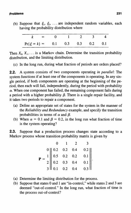
Problems 231
(b) Suppose that Z Z,, . . . are independent random variables, eachhaving the probability distribution where
k = 0 1 2 3 4
Pr{e = k} = 0.1 0.3 0.3 0.2 0.1
Then X0, X,, ... is a Markov chain. Determine the transition probabilitydistribution, and the limiting distribution.
(c) In the long run, during what fraction of periods are orders placed?
2.2. A system consists of two components operating in parallel: Thesystem functions if at least one of the components is operating. In any sin-gle period, if both components are operating at the beginning of the pe-riod, then each will fail, independently, during the period with probabilitya. When one component has failed, the remaining component fails duringa period with a higher probability /3. There is a single repair facility, andit takes two periods to repair a component.
(a) Define an appropriate set of states for the system in the manner ofthe Reliability and Redundancy example, and specify the transitionprobabilities in terms of a and /3.
(b) When a = 0.1 and /i = 0.2, in the long run what fraction of timeis the system operating?
2.3. Suppose that a production process changes state according to a
Markov process whose transition probability matrix is given by
0 1 2 3
0 0.2 0.2 0.4 0.2
1 0.5 0.2 0.2 0.1P
2 0.2 0.3 0.4 0.1
3 0.1 0.2 0.4 0.3
(a) Determine the limiting distribution for the process.(b) Suppose that states 0 and 1 are "in-control," while states 2 and 3 are
deemed "out-of-control." In the long run, what fraction of time isthe process out-of-control?
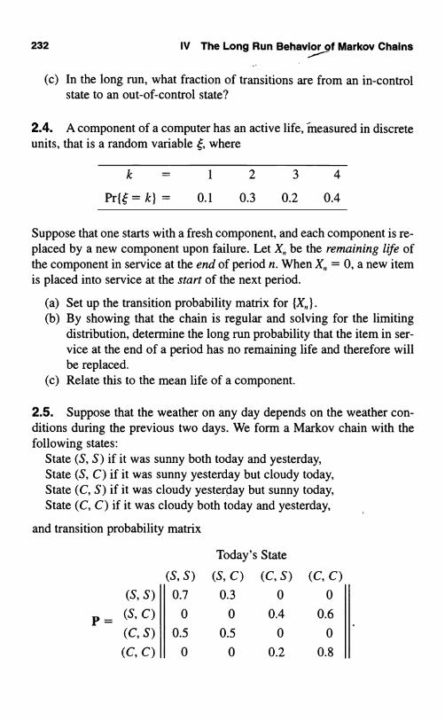
232 IV The Long Run Behav!"f Markov Chains
(c) In the long run, what fraction of transitions are from an in-controlstate to an out-of-control state?
2.4. A component of a computer has an active life, measured in discreteunits, that is a random variable , where
k = 1 2 3 4
Pr{f = k} = 0.1 0.3 0.2 0.4
Suppose that one starts with a fresh component, and each component is re-placed by a new component upon failure. Let X,, be the remaining life ofthe component in service at the end of period n. When X,, = 0, a new itemis placed into service at the start of the next period.
(a) Set up the transition probability matrix for(b) By showing that the chain is regular and solving for the limiting
distribution, determine the long run probability that the item in ser-vice at the end of a period has no remaining life and therefore willbe replaced.
(c) Relate this to the mean life of a component.
2.5. Suppose that the weather on any day depends on the weather con-ditions during the previous two days. We form a Markov chain with thefollowing states:
State (S, S) if it was sunny both today and yesterday,State (S, C) if it was sunny yesterday but cloudy today,State (C, S) if it was cloudy yesterday but sunny today,State (C, C) if it was cloudy both today and yesterday,
and transition probability matrix
Today's State
(S, S) (S, C) (Cl S) (C, C)
(S,S) 0.7 0.3 0 0
P= (S,C) 0 0 0.4 0.6
(C, S) 0.5 0.5 0 0
(Cl C) 0 0 0.2 0.8

Problems 233
-(a)Given that it is sunny on days 0 and 1, what is the probability it issunny on day 5?
(b) In the long run, what fraction of days are sunny?
2.6. Consider a computer system that fails on a given day with proba-bility p and remains "up" with probability q = 1 - p. Suppose the repairtime is a random variable N having the probability mass function p(k) =/3(1 fork= 1,2,...,where0<8< 1.LetX,, = 1 ifthecom-puter is operating on day n and X,, = 0 if not. Show that {X,, } is a Markovchain with transition matrix
0 1
and a = 1 - /3. Determine the long run probability that the computer isoperating in terms of a, /3, p, and q.
2.7. Customers arrive for service and take their place in a waiting line.There is a single service facility, and a customer undergoing service at thebeginning of a period will complete service and depart at the end of theperiod with probability (3 and will continue service into the next periodwith probability a = 1 - /3, and then the process repeats. This descriptionimplies that the service time q of an individual is a random variable withthe geometric distribution,
Pr{rl = k} = /3ak-' for k = 1, 2, ... ,and the service times of distinct customers are independent random vari-ables.
At most a single customer can arrive during a period. We suppose thatthe actual number of arrivals during the nth period is a random variabletaking on the values 0 or 1 according to
=pand
Pr(,= 1}=q=1-p forn = 0, 1, . . . .
The state X,, of the system at the start of period n is defined to be thenumber of customers in the system, either waiting or being served. Then
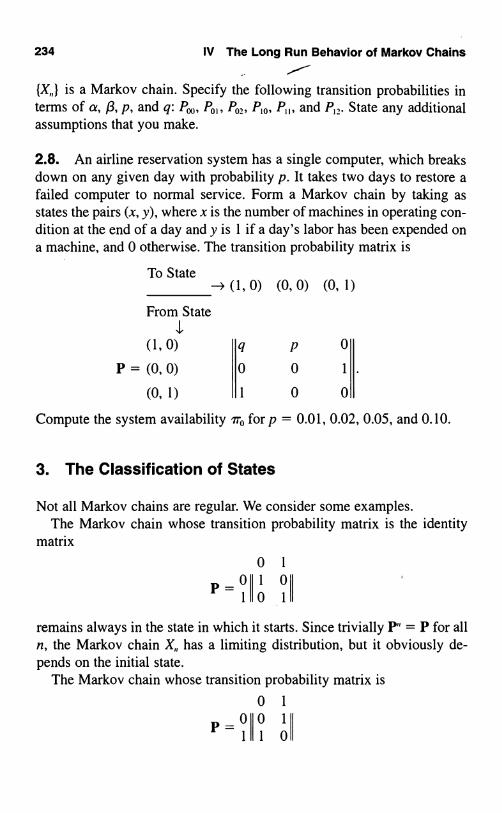
234 IV The Long Run Behavior of Markov Chains
is a Markov chain. Specify the following transition probabilities interms of a, /3, p, and q: P. PO , P02, P,p, P, and P,,. State any additionalassumptions that you make.
2.8. An airline reservation system has a single computer, which breaksdown on any given day with probability p. It takes two days to restore afailed computer to normal service. Form a Markov chain by taking asstates the pairs (x, y), where x is the number of machines in operating con-dition at the end of a day and y is 1 if a day's labor has been expended ona machine, and 0 otherwise. The transition probability matrix is
To State-4 (1, 0) (0, 0) (0, 1)
From StateI
(1,0) q p 0
P = (0, 0) 0 0 1
(0, 1) 1 0 0
Compute the system availability iro for p = 0.01, 0.02, 0.05, and 0.10.
3. The Classification of States
Not all Markov chains are regular. We consider some examples.The Markov chain whose transition probability matrix is the identity
matrix
P=0
0 1
1 0
0 1
remains always in the state in which it starts. Since trivially P" = P for alln, the Markov chain X,, has a limiting distribution, but it obviously de-pends on the initial state.
The Markov chain whose transition probability matrix is
0 1
P=01010

3. The Classification of States 235
oscillates deterministically between the two states. The Markov chain isperiodic, and no limiting distribution exists. When n is an odd number,then P" = P, but when n is even, then P" is the 2 X 2 identity matrix.
When P is the matrix
0 1
0 2P 1110z
1'
P" is given by
P" = 01
1
0 1
(z)" 1 - (z ),f0 1
and the limit is
lim P" =
0 1
0110 1
1 0 1
Here state 0 is transient; after the process starts from state 0, there is apositive probability that it will never return to that state.
The three matrices just presented illustrated three distinct types of be-havior in addition to the convergence exemplified by a regular Markovchain. Various and more elaborate combinations of these behaviors arealso possible. Some definitions and classifications of states and matricesare needed in order to sort out the variety of possibilities.
3.1. Irreducible Markov Chains
Since j is said to be accessible from state i if P;' > 0 for some integern ? 0; i.e., state j is accessible from state i if there is positive probabilitythat state j can be reached starting from state i in some finite number oftransitions. Two states i and j, each accessible to the other, are said to com-municate, and we write i H j. If two states i and j do not communicate,then either
P;;' = 0 for all n >- 0

236 IV The-Long Run Behavior of Markov Chains
or
P%;') = 0 for all n ::,-0
or both relations are true. The concept of communication is an equiva-lence relation:
(i) i H i (reflexivity), a consequence of the definition of
(1 =j,P1)=S;;=10 i j
(ii) If i t--* j, then j t4 i (symmetry), from the definition of communi-cation.
(iii) If i H j and j t-4 k, then i H k (transitivity).
The proof of transitivity proceeds as follows: i <-4j and j H k imply thatthere exist integers n and m such that P;) > 0 and P;'k)> 0. Consequently,by the nonnegativity of each P;,), we conclude that
kP('?) P('11) p(,n) > 0.it rk ii ik
x
r=0
A similar argument shows the existence of an integer v such that Pki°) > 0,as desired.
We can now partition the totality of states into equivalence classes. Thestates in an equivalence class are those that communicate with each other.It may be possible starting in one class to enter some other class with pos-itive probability; if so, however, it is clearly not possible to return to theinitial class, or else the two classes would together form a single class. Wesay that the Markov chain is irreducible if the equivalence relation inducesonly one class. In other words, a process is irreducible if all states com-municate with each other.
To illustrate this concept, we consider the transition probability matrix
a a
0 0 0
0 0 0
P 0 0 0 1 0
0 0 0 z
0 0.0 1 0
P 0.00 P°I

3. The Classification of States 237
where P, is an abbreviation for the matrix formed from the initialtwo rows and columns of P, and similarly for P2. This Markov chainclearly divides into the two classes composed of states (1, 2) and states{3,4,5}.
If the state of Xo lies in the first class, then the state of the system there-after remains in this class, and for all purposes the relevant transition ma-trix is P. Similarly, if the initial state belongs to the second class, then therelevant transition matrix is R. This is a situation where we have twocompletely unrelated processes labeled together.
In the random walk model with transition matrix
states
1 0 0 0 0 0 0 0
q 0 p 0 0 0 0 1
0 q 0 p 0 0 0 2P= (3.1)
0 ... q 0 p a-1
0 ... 0 0 1 a
we have the three classes (0), 11, 2, . . . , a - 1), and {a}. In this exampleit is possible to reach the first class or third class from the second class,but it is not possible to return to the second class from either the first orthe third class.
3.2. Periodicity of a Markov Chain
We define the period of state i, written d(i), to be the greatest common di-visor (g.c.d.) of all integers n ? 1 for which P;;'' > 0. [If P;;' = 0 for alln ? 1, define d(i) = 0.] In a random walk (3.1), every transient state1, 2, ... , N - 1 has period 2. If P; > 0 for some single state i, then thatstate now has period 1, since the system can remain in this state any lengthof time.
In a finite Markov chain of n states with transition matrix

238 IV The Long Run Behavior of Markov Chains
n
0 1 0 0
0 0 1 0 0
P=0 0 1
1 0 0 0
each state has period n.Consider the Markov chain whose transition probability matrix is
0 1 2 3
0 0 1 0 0
1 0 0 1 0P=
2 0 0 0 1
3 z 0 2 0
We evaluate P.=0,P'.1) =0,P'1'=0,P11=1,P1,10) = 0,P1,1) =;. The setof integers n ? 1 for which P > 0 is {4, 6, 8, ... }. The period of state 0is d(0) = 2, the greatest common divisor of this set.
Example Suppose that the precipitation in a certain locale depends onthe season (Wet or Dry) as well as on the precipitation level (High, Low)during the preceding season. We model the process as a Markov chainwhose states are of the form (x, y), where x denotes the season (W = Wet,D = Dry) and y denotes the precipitation level (H = High, L = Low).Suppose the transition probability matrix is
(W, H) (W, L) (D, H) (D, L)
(W, H) 0 0 0.8 0.2
P= (W,L)0 0 0.4 0.6
(D, H) 0.7 0.3 0 0
(D, L) 0.2 0.8 0 0
All states are periodic with period d = 2.
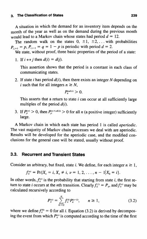
3. The Classification of States 239
A situation in which the demand for an inventory item depends on themonth of the year as well as on the demand during the previous monthwould lead to a Markov chain whose states had period d = 12.
The random walk on the states 0, ± 1, ±2, . . . with probabilitiesP;.i+, = p, P,, = q = I - p is periodic with period d = 2.
We state, without proof, three basic properties of the period of a state:
1. If i t-- j then d(i) = d(j).
This assertion shows that the period is a constant in each class ofcommunicating states.
2. If state i has period d(i), then there exists an integer N depending oni such that for all integers n ? N,
p;ud<<» > 0.
This asserts that a return to state i can occur at all sufficiently largemultiples of the period d(i).
3. If P;' > 0, then P;"+" > 0 for all n (a positive integer) sufficientlylarge.
A Markov chain in which each state has period 1 is called aperiodic.The vast majority of Markov chain processes we deal with are aperiodic.Results will be developed for the aperiodic case, and the modified con-clusions for the general case will be stated, usually without proof.
3.3. Recurrent and Transient States
Consider an arbitrary, but fixed, state i. We define, for each integer n ? 1,
i, v= 1,2,...,n- 1X0=i}.In other words, f,;" is the probability that starting from state i, the first re-turn to state i occurs at the nth transition. Clearly f,!;" = P;;, and f °i' may becalculated recursively according to
P(n) =n ? 1, (3.2)
k=O
where we define f ' = 0 for all i. Equation (3.2) is derived by decompos-ing the event from which P;;" is computed according to the time of the first

240 IV The Long Run Behavior of Markov Chains
return to state i. Indeed, consider all the possible realizations of theprocess for which X0 = i, X,, = i, and the first return to state i occurs at thekth transition. Call this event Ek. The events Ek (k = 1, 2, ... , n) areclearly mutually exclusive. The probability of the event that the first re-turn is at the kth transition is by definition f k). In the remaining n - k tran-sitions, we are dealing only with those realizations for which X,, = i.Using the Markov property, we have
Pr{Ek} = Pr{first return is at kth transitionlX0 = i} Pr{X = iIXk = i}
{(k) n-k)-Jii iii 1<k-<n
(recall that P° = 1). Hence,r
Pr(X = i X = i Pr(E. (k) -k) _ (k)P(n-k)l rr 10 }- l k} - f ii u f ii n
k=1 k=1 k=0
since by definition f ;°j = 0. The verification of (3.2) is now complete.When the process starts from state i, the probability that it returns to
state i at some time is
Jii f ii N-' f ii=o =o
(3.3)
We say that a state i is recurrent if fi = 1. This definition says that a statei is recurrent if and only if, after the process starts from state i, the proba-bility of its returning to state i after some finite length of time is one. Anonrecurrent state is said to be transient.
Consider a transient state i. Then the probability that a process startingfrom state i returns to state i at least once is fi < 1. Because of the Markovproperty, the probability that the process returns to state i at least twice is(fi )2, and repeating the argument, we see that the probability that theprocess returns to i at least k times is (fi)k for k = 1, 2, .... Let M be therandom variable that counts the number of times that the process returnsto i. Then we have shown that M has the geometric distribution in which
and
Pr{M?kjX0=i} =(fii)k fork= 1,2,... (3.4)
= f,E i 3 5[ 0 ]1 -,fi
( . )

3. The Classification of States 241
Theorem 3.1 establishes a criterion for the recurrence of a state i interms of the transition probabilities P(i"'.
Theorem 3.1 A state i is recurrent if and only ifx
"ii)
= 00.`n=1
Equivalently, state i is transient if and only if P;") < oo.
Proof Suppose first that state i is transient so that, by definition, fi < 1,and let M count the total number of returns to state i. We write M in termsof indicator random variables as
where
1(X = i},
1
={0if
X 0 i.
Now, equation (3.5) shows that E[MIXo = i] < oo when i is transient. Butthen
xoo > E[MI Xo = i] = E[1(X = i) I Xo = i]
x
`ii"),11=1
as claimed.Conversely, suppose Pi;"' < oo. Then M is a random variable whose
mean is finite, and thus M must be finite. That is, starting from state i, theprocess returns to state i only a finite number of times. Then there must bea positive probability that, starting from state i, the process never returnsto that state. In other words I - fii > 0 or fi < 1, as claimed.
Corollary 3.1 If i H j and if i is recurrent, then j is recurrent.

242 IV The Long Run Behavior of Markov Chains
Proof Since i <-4j, there exists m, n ? 1 such that
P;") > 0 and P,',") > 0.
Let v > 0. We obtain, by the usual argument (see Section 3.1),P("'+"+°) P1 ;"')P;°)Pf") and, on summing,
x x+(m+it+v)P
v=o V=o
) m)P(OP(n) = P(m)P(n)P)
Hence if V'=o P;'> diverges, then P;") also diverges. 11
This corollary proves that recurrence, like periodicity, is a class prop-erty; that is, all states in a equivalence class are either recurrent ornonrecurrent.
Example Consider the one-dimensional random walk on the positiveand negative integers, where at each transition the particle moves withprobability p one unit to the right and with probability q one unit to theleft (p + q = 1). Hence
pn n!n!
We appeal now to Stirling's formula (see 1, (6.10)),
n! ,r W+in-e-'.
Applying (3.7) to (3.6), we obtain
(3.6)
(3.7)
It is readily verified that p(1 - p) = pq <_ , with equality holding if andonly if p = q = 2. Hence Pte' = oc if and only if p = ;. Therefore, fromTheorem 3.1, the one-dimensional random walk is recurrent if and only ifp = q = Remember that recurrence is a class property. Intuitively, ifp q, there is positive probability that a particle initially at the origin willdrift to +cc if p > q (to -o if p < q) without ever returning to the origin.

Exercises 243
Exercises
3.1. A Markov chain has a transition probability matrix
0 1 2 3 4 5 6 70 0 1 0 0 0 0 0 01 0 0 1 0 0 0 0 02 0 0 0 1 0 0 0 03 0 0 0 0 1 0 0 04 0.5 0 0 0 0 0.5 0 05 0 0 0 0 0 0 1 0
6 0 0 0 0 0 0 0 1
7 1 0 0 0 0 0 0 0
For which integers n = 1, 2, ..., 20 is it true that
P%) > 0?
What is the period of the Markov chain?
Hint: One need not compute the actual probabilities. See Section 1.1.
3.2. Which states are transient and which are recurrent in the Markovchain whose transition probability matrix is
0 1 2 3 4
0 0 0
1 1 1 0 02 4 4
0 0 0 0 1
1 1 1 004 4 4
0 0 1 0 0
0 0 0 0 0
7

244 IV The Long Run Behavior of Markov Chains
3.3. A Markov chain on states 10, 1, 2, 3, 4, 5} has transition probabil-ity matrices
(a)
(b)
1
0
0
0
Find all communicating classes.
20 0
3 04
0 0
4 05
0 44
1 1
6 6
0 0 0
0 0 0
0 0 0
I 3 08 8
04 4
0 0 1
3.4. Determine the communicating classes and period for each state ofthe Markov chain whose transition probability matrix is
0 1 2 3 4 5
0 0 0 0 ; 0
1 0 0 1 0 0 0
2 0 0 0 1 0 0
3 0 0 0 0 1 0
4 0 0 0 0 0 1
5 0 0 3 13 0 3

4. The Basic Limit Theorem of Markov Chains 245
Problems
3.1. A two state Markov chain has the transition probability matrix
P=00 1
I1a
b 1-ba
(a) Determine the first return distribution
(b) Verify equation (3.2) when i = 0. (Refer to III, (5.2).)
3.2. Show that a finite state aperiodic irreducible Markov chain is regu-lar and recurrent.
3.3. Recall the first return distribution (Section 3.3)
J"'=Pr{X,
0 by convention. Using equation (3.2), determine f', n = 1, 2,3, 4, 5, for the Markov chain whose transition probability matrix is
0 1 2 3
0 0 '2 0 '2
1 0 0 1 0
2 0 0 0 1
3 z 0 0 z
4. The Basic Limit Theorem of Markov Chains
Consider a recurrent state i. Then
f;;''= Pr{X = i,X, i for v= 1,...,n - 11X°= i} (4.1)
is the probability distribution of the first return time
R; = min( n ? 1; X = i). (4.2)

246 IV The Long Run Behavior of Markov Chains
This is
f = Pr{R; = njXo = i } for n = 1, 2, .... (4.3)
Since state i is recurrent by assumption, then f; _ I", f;'' = 1, and R; isa finite-valued random variable. The mean duration between visits to statei is
m; = E[R;IXO = i] = 7, nfj'. (4.4)/1 = 1
After starting in i, then, on the average, the process is in state i once everym; = E[R;IXO = i] units of time. The basic limit theorem of Markov chainsstates this result in a sharpened form.
Theorem 4.1 The basic limit theorem of Markov chains(a) Consider a recurrent irreducible aperiodic Markov chain. Let
P' be the probability of entering state i at the nth transition, n = 0, 1,2, . . . , given that X0 = i (the initial state is i). By our earlier convention
1. Let f;," be the probability of first returning to state i at the nthtransition, n = 0, 1 , 2, ... , where f ;;°' = 0. Then,
lim 1t" =',=
1 1
fcI mr
(b) under the same conditions as in (a), Pi;'ll = P;"'for allstates j.
Remark Let C be a recurrent class. Then P,"' = 0 for i E C, j (4 C, andevery n. Hence, once in C it is not possible to leave C. It follows that thesubmatrix JIPJI, i, j E C, is a transition probability matrix and the associ-ated Markov chain is irreducible and recurrent. The limit theorem, there-fore, applies verbatim to any aperiodic recurrent class.
If lim,,. P,;"I > 0 for one i in an aperiodic recurrent class, then 9T; > 0for all j in the class of i. In this case, we call the class positive recurrentor strongly ergodic. If each ?r; = 0 and the class is recurrent, we speak ofthe class as null recurrent or weakly ergodic. In terms of the first returntime R; = min { n ? 1; X = i } , state i is positive recurrent if m; _E[R;IXQ = i] < c and null recurrent if m; = °. This statement is immedi-ate from the equality lim,,. P;;"' = ir; = 1/m;. An alternative method for

4. The Basic Limit Theorem of Markov Chains 247
determining the limiting distribution ?r, for a positive recurrent aperiodicclass is given in Theorem 4.2.
Theorem 4.2 In a positive recurrent aperiodic class with states j = 0,1,2,...,
limPJ"='7r,=2. 'TiPipi=0 i=0
= 1,
and the ir's are uniquely determined by the set of equationsx x
ir,?0, , ir,= 1, and ir,P; forj = 0, 1, . . . . (4.6)1=0 r=0
Any set (i71);_0 satisfying (4.6) is called a stationary probability distri-bution of the Markov chain. The term "stationary" derives from the prop-erty that a Markov chain started according to a stationary distribution willfollow this distribution at all points of time. Formally, if Pr{Xo = i} = 1rthen Pr{X = i} = 1r, for all n = 1, 2, .... We check this for the casen = 1; the general case follows by induction. We write
Pr{X1 = i} > Pr{Xo = k) Pr{X1 = iIX0 = k}k=0X
k=01r,P = IT,,
where the last equality follows because 7r = (1r, 1r ...) is a stationarydistribution. When the initial state X is selected according to the station-ary distribution, then the joint probability distribution of (X,,, is givenby
Pr (X,, = i, X,,, = j) = 7r,P,,.
The reader should supply the proof.A limiting distribution, when it exists, is always a stationary distribu-
tion, but the converse is not true. There may exist a stationary distributionbut no limiting distribution. For example, there is no limiting distributionfor the periodic Markov chain whose transition probability matrix is
P=°011'
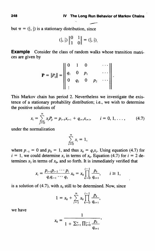
248 IV The Long Run Behavior of Markov Chains
but it = (;,;)
is a stationary distribution, since
0 1
1 0
Example Consider the class of random walks whose transition matri-ces are given by
P = IIP;II =
1 =xo+IxoF1 Pk ,
P2
This Markov chain has period 2. Nevertheless we investigate the exis-tence of a stationary probability distribution; i.e., we wish to determinethe positive solutions of
x; = Z, x;P;, = P,-,x,-1 + q,+,x,+,, i = 0, 1, ... , (4.7)i=o
under the normalization
i=o
where p-, = 0 and po = 1, and thus xo = q,x,. Using equation (4.7) fori = 1, we could determine x2 in terms of xo. Equation (4.7) for i = 2 de-termines x3 in terms of xo, and so forth. It is immediately verified that
r-iP,-,P,-2 xo = xo Pk
q,q,-, q, k=O qk+,
is a solution of (4.7), with xo still to be determined. Now, since
i-I
we have
0 1 0
q, 0 P,
0 q2 0
i=1
1
xo =1 + E;_, IIk o Pk
qk+,

4. The Basic Limit Theorem of Markov Chains 249
and so
x i-lxo>Oifandonly if> f Pk <oo.
i=1 k=o qk+l
In particular, if Pk = p and qk = q = 1 - p fork ? 1, the series
x (-i 1 xr
i=1 k oqk+l P=\q/converges only when p < q, and then
plq1Z(p)1/ -Pr=i q P Pq q-P
and
xo = l+l/(q-p) 1+q-p 2(q)'xk = p1 1 xo = Zp (1
- q) q )kfor k = 1, 2, ... .
q
Example Consider now the Markov chain that represents the successruns of binomial trials. The transition probability matrix is
Po
P,
A
1-pa 0 0
0 1-p, 0
0 0 1-P2(0<pk<1).
The states of this Markov chain all belong to the same equivalence class(any state can be reached from any other state). Since recurrence is a classproperty (see Corollary 3.1), we will investigate recurrence for the zerothstate.
Let R. = min{n ? 1; X = 0} be the time of first return to state 0. It iseasy to evaluate

250 IV The Long Run Behavior of Markov Chains
Pr {Ro > 11X0 = 01 = (1 - Po),
Pr(R0 > 21X0 = 0) = (1 - Po)(l - Pi),
Pr{Ro > 31X0 = 0) = (1 - NO - Pi)(1 - P2),
k-1
Pr{R0 > k1 Xo = 0) = (1 - Po)(1 - Pi) ... (I - Pk-t) = 11i=o
In terms of the first return distribution
foo =Pr(RO=nIX0=0),
we have
Pr{Ro > k1Xo = 0) =
or
f 11,0E0 ,
(I - Pr).
k k-1
foo = I - Pr(Ro > klX0 = 0) = 1 - fl (1 - p;).,,=1 ;=O
By definition, state 0 is recurrent provided I,,_, ff' = 1. In terms ofpo, pl, ... then, state 0 is recurrent whenever "Mk.. IIk=o (1 - p) _I1;=, (1 - p;) = 0. Lemma 4.1 shows that II o (I - p;) = 0 is equivalent,in this case, to the condition Y,;_ p; = oo.
Lemma4.1 If0<p;<1,i=0, 1,2,...,then u,, =H o(1 -p;)-0as in - 00 if and only if t, =o p; = oo.
Proof Assume J o p; = co. Since the series expansion for exp(-p;) isan alternating series with terms decreasing in absolute value, we can write
1 - P, < 1 - P; +P 3l + ... = exp(-Pr), i = 0, 1, 2..... (4.8)2! 3!
Since (4.8) holds for all i, we obtain II;"=o (1 - p;) < exp(-I;"o p;). Butby assumption,
'II
1im,,,_*t ;=o
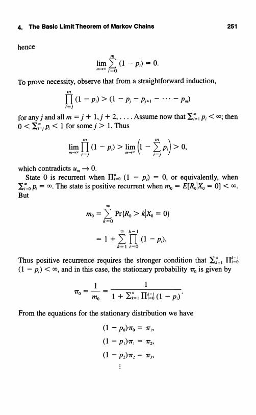
4. The Basic Limit Theorem of Markov Chains 251
hence
in
lim 7, (1 - pi) = 0.m-,- 1=0
To prove necessity, observe that from a straightforward induction,n:
Fl(1-pi)>(1-pi-pi.,-...-P.)
i=i
for any j and all m = j + 1, j + 2..... Assume now that J;_, pi < oo; then0 < p, < 1 for some j > 1. Thus
m m
lim F1 (1 - p;) > lim (1 - p) ,
which contradicts u,,, -* 0.State 0 is recurrent when II;=o (1 - pi) = 0, or equivalently, when
Ji=o p; = oo. The state is positive recurrent when mo = E[RoIXQ = 0] < oo.But
mo = I Pr(R0 > kIX0 = 0)k=0
x k-1= 1 +Ifl(1-pi).
Thus positive recurrence requires the stronger condition that Ik=, IIk=o(1 - pi) < oo, and in this case, the stationary probability 7r0 is given by
IT0
m0 1 + Yk=1 llk=0 (1 Pi)
From the equations for the stationary distribution we have
(1 - P0)1T0 = IT1,
(1-P1)7r,=7r,,(1 - P2)7r2 = 1rs,

252 IV The Long Run Behavior of Markov Chains
or
IT, = (I - Po) lo,
172 = (I - P1)1Ti = (I - Pi)(' - Po)lTo,
177 = (I - P2)1r2 = (I - P2)(1 - PA)(I - Po)17o,
and, in general,k-1
Irk=7ro F1 (1 -p) fork? 1.i=o
In the special case where p, = p = 1 - q for i = 0, 1, ... , thenkII;=o (I -Pi)=q,
x 1
mo= 1 + qk=-,k=1 P
so that irk = pqk for k = 0, 1, ... .
Remark Suppose ao, a,, a2i ... is a convergent sequence of real num-bers where a - a as n - oo. Then it can be proved by elementary meth-ods that the partial averages of the sequence also converge in the form
1 J, - 1
lim - 7 ak = a.n k=0
(4.9)
Applying (4.9) with a,, = P,;'', where i is a member of a positive recurrentaperiodic class, we obtain
1 n-, IJim -7 P,o"'=7r,=->0,,t-," n,,=o m,
(4.10)
where 7r = (7ro, 7r,, ...) is the stationary distribution and where m, is themean return time for state i. Let M;"' be the random variable that countsthe total number of visits to state i during time periods 0, 1, ... , n - 1.
We may write
n-I
M;"'=> 1(Xk=i},k=0
(4.11)
where

4. The Basic Limit Theorem of Markov Chains 253
1 if Xk = i,Ilk = i } = 10
if Xk = i, (4.12)
and then see that
n-' n-i
E[M;")IXo = i] = 7 E[1{Xk = i}IX0 = i] _ P,;k). (4.13)k=0
Then, referring to (4.10), we have
1 1
k=0
lim - E[M;")I XO = i] - (4.14)"- n m;
In words, the long run (n -> c) mean visits to state i per unit time equals7r;, the probability of state i under the stationary distribution.
Next, let r(i) define a cost or rate to be accumulated upon each visit tostate i. The total cost accumulated during the first n stages is
n-I n-IRc"-"
= 7- r(Xk) = 7, 7 1 {X4. = i } r(i)k=0 k=0
W
_ M;")r(i).
i=0
i
(4.15)
This leads to the following derivation showing that the long run mean costper unit time equals the mean cost evaluated over the stationary distribu-tion:
lim 1 E[R°'-')IX0 = i] = limI
E[M;")IXO = i]r(i)n "-Ix l=() n
ir,r(i).i=0
(4.16)
(When the Markov chain has an infinite number of states, then thederivation requires that a limit and infinite sum be interchanged. A suf-ficient condition to justify this interchange is that r(i) be a bounded func-tion of i.)
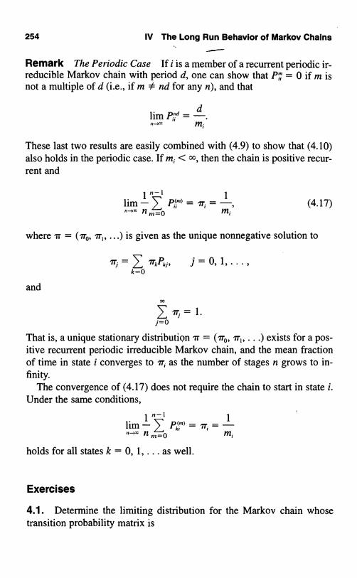
254 IV The Long Run Behavior of Markov Chains
Remark The Periodic Case If i is a member of a recurrent periodic ir-reducible Markov chain with period d, one can show that P;;' = 0 if m isnot a multiple of d (i.e., if m : nd for any n), and that
limP;nd=d
.n-ax
m,
These last two results are easily combined with (4.9) to show that (4.10)also holds in the periodic case. If m; < oo, then the chain is positive recur-rent and
1im-"-'" n,,,=o
(4.17)
where 'rr = (iro, Ir ...) is given as the unique nonnegative solution to
k=0j=0,1,...,71kPkj,
and
= 1.
j=0
That is, a unique stationary distribution 'rr = (Iro, ir,, ...) exists for a pos-itive recurrent periodic irreducible Markov chain, and the mean fractionof time in state i converges to ir; as the number of stages n grows to in-finity.
The convergence of (4.17) does not require the chain to start in state i.Under the same conditions,
1- ,
lim-7 Pk;"'=;_--,= n ,,,=o mi
holds for all states k = 0, 1.... as well.
Exercises
4.1. Determine the limiting distribution for the Markov chain whosetransition probability matrix is

Exercises 255
0 1 2 3 4
0 g p 0 0 0
1 g 0 p 0 0
p=2 g 0 0 p 0
3 g 0 0 0 p
4 1 0 0 0 0
wherep > 0, q > 0, andp + q = 1.
4.2. Consider the Markov chain whose transition probability matrix isgiven by
0 1 2 3
0 0 1 0 0
1 0.1 0.4 0.2 0.3P=
2 0.2 0.2 0.5 0.1
3 0.3 0.3 0.4 0
(a) Determine the limiting probability .7ro that the process is in state 0.(b) By pretending that state 0 is absorbing, use a first step analysis (III,
Section 4) and calculate the mean time m,0 for the process to gofrom state 1 to state 0.
(c) Because the process always goes directly to state 1 from state 0, themean return time to state 0 is m = 1 + m,,,. Verify equation (4.5),ir = 1/NO.
4.3. Determine the stationary distribution for the periodic Markov chainwhose transition probability matrix is
0 1 2 3
0110 0 112 2
0 0
0 0
0 2 0

256 IV The Long Run Behavior of Markov Chains
Problems
4.1. Consider the Markov chain on (0, 1} whose transition probabilitymatrix is
0 1
Oll al a/ill' 0<a,/3<1.
(a) Verify that (Iro, ir,) = ((3/(a + /3), al(a + (3)) is a stationary distri-bution.
(b) Show that the first return distribution to state 0 is given by f.(') _(1 - a) and f . " ' ) = a/3(1 - /3)i-2 f o r n = 2, 3, ... .
(c) Calculate the mean return time mo = Y,'_, nff'' and verify thatTrp = 1 /mo.
4.2. Determine the stationary distribution for the Markov chain whosetransition probability matrix is
0 1 2 3
0 0 0 2 2
1 20 0 3 3P
I 32 4 4 0 0
1 23 3 3 0 0
4.3. Consider a random walk Markov chain on state 0, 1, ... , N withtransition probability matrix
0 1 2 3 4 5 N- 1 N0 0 1 0 0 0 0 0 0
1 q, 0 p, 0 0 0 0 0
2 0 q2 0 P2 0 0 ... 0 0
3 0 0 q3 0 P3 0 ... 0 0
N-1 0 0 0 0 0 0 0 PN- I
N 0 0 0 0 0 0

Problems 257
where pi +q; = l,pi> O,q;> 0foralli.The transition probabilities from state 0 and N "reflect" the process
back into state 1, 2, . . . , N - 1. Determine the limiting distribution.
4.4. Let {a; : i = 1, 2, ...} be a probability distribution, and considerthe Markov chain whose transition probability matrix is
0 1 2 3 4 5
0 a, a, a, a4 a5 a6
1 1 0 0 0 0 0
2 0 1 0 0 0 0
3 0 0 1 0 0 0
4 0 0 0 1 0 0
What condition on the probability distribution { a; : i = 1, 2, ... } is nec-essary and sufficient in order that a limiting distribution exist, and what isthis limiting distribution? Assume a, > 0 and a2 > 0, so that the chain isaperiodic.
4.5. Let P be the transition probability matrix of a finite state regularMarkov chain. Let M = Ilm;jll be the matrix of mean return times.
(a) Use a first step argument to establish that
mj=1+ Pkmk j.k*j
(b) Multiply both sides of the preceding by ir, and sum to obtain
k*j i
7r,Pkmkj.
Simplify this to show (see equation (4.5))
Trjm,, = 1, or irj = 1/m;;.
4.6. Determine the period of state 0 in the Markov chain whose transi-tion probability matrix is

258 IV The Long Run Behavior of Markov Chains
3 2 1 0 -1 -2 -3 -4
3 0 0 0 1 0 0 0 0
2 1 0 0 0 0 0 0 0
1 0 1 0 0 0 0 0 0
0 0 0 2 0 2 0 0 0P=-1 0 0 0 0 0 1 0 0
-2 0 0 0 0 0 0 1 0
-3 0 0 0 0 0 0 0 1
-4 0 0 0 1 0 0 0 0
4.7. An individual either drives his car or walks in going from his hometo his office in the morning, and from his office to his home in the after-noon. He uses the following strategy: If it is raining in the morning, thenhe drives the car, provided it is at home to be taken. Similarly, if it is rain-ing in the afternoon and his car is at the office, then he drives the carhome. He walks on any morning or afternoon that it is not raining or thecar is not where he is. Assume that, independent of the past, it rains dur-ing successive mornings and afternoons with constant probability p. In thelong run, on what fraction of days does our man walk in the rain? What ifhe owns two cars?
4.8. A Markov chain on states 0, 1, . . . has transition probabilities
forj=0, 1,...,i,i+ 1.
Find the stationary distribution.
5. Reducible Markov Chains*
Recall that states i and j communicate if it is possible to reach state j start-ing from state i, and vice versa, and a Markov chain is irreducible if all
* The overwhelming majority of Markov chains encountered in stochastic modeling areirreducible. Reducible Markov chains form a specialized topic.

5. Reducible Markov Chains 259
pairs of states communicate. In this section we show, mostly by example,how to analyze more general Markov chains.
Consider first the Markov chain whose transition probability matrix is
which we write in the form
where
P, _
I 1
2 2
I 3
4 4
P- I OI P" 11,
and P, =1 2
3 3
2 ,
3 3
The chain has two communicating classes, the first two states forming oneclass and the last two states forming the other. Then
P2 =
and, in general,
I I
2 2
1 3
4 4
0 0
0 0
3 5
8 8
5 ,I
16 16
0 0
0 0
P" =
0 0
0 0
1 2
3 3
2I
3 3
x
I I
2 2
I 3
4 4
0 0
0 0
0 0
0 05 4
9 9
4 5
9 9
P;t 00 P"
2
0 0
0 01 2
3 3
2 I
3 3
P; 0
0 Pz
n ? 1. (5.1)

260 IV The Long Run Behavior of Markov Chains
Equation (5.1) is the mathematical expression of the property that it is notpossible to communicate back and forth between distinct communicatingclasses; once in the first class the process remains there thereafter; andsimilarly, once in the second class, the process remains there. In effect,two completely unrelated processes have been labeled together. The tran-sition probability matrix P is reducible to the irreducible matrices PI andP2. It follows from (5.1) that
limp" =-+x
where
limp;' _7r0') ?Ti' )
l 1)?To') ITand limp" _
lro'
I0(2)
We solve for 7T(" = (7r."), ?T(,") and ir(2' _ (aro22), 7T 2)) in the usual way:
27T0 +47T1 7T0
1 (1) i (I) = (1)7TO + - 7T 7Ti
IT0(1) + IT( 11)= 1,
or
1 ,71)=20 3s 1 3s (5.2)
and because P2 is doubly stochastic (see Section 1.1), it follows that1, X12) = 1
The basic limit theorem of Markov chains, Theorem 4.1, referred to anirreducible Markov chain. The limit theorem applies verbatim to anyaperiodic recurrent class in a reducible Markov chain. If i, j are in the sameaperiodic recurrent class, then P"' - 1/m; > 0 as n - cc. If i, j are in thesame periodic recurrent class, then n-' 11 =0 P' -4 1/m; ? 0 as n -' oo.
If j is a transient state, then P")-40
as n -4 oc, and, more generally,P;'' -4 0 as n -4 oo for all initial states i.

5. Reducible Markov Chains 261
In order to complete the discussion of the limiting behavior of P;"', westill must consider the case where i is transient and j is recurrent. Considerthe transition probability matrix
0 1 2 3
0 2 2 0 0
1 4 4 0 0P=
2 4 4 4 4
3 0 0 0 1
There are three classes: 10, 1}, {2), and {3 }, an d of these (0, 11 and {3) arerecurrent, while (2) is transient. Starting from state 2, the process ulti-mately gets absorbed in one of the other classes. The question is, Whichone? or more precisely, What are the probabilities of absorption in the tworecurrent classes starting from state 2?
A first step analysis answers the question. Let u denote the probabilityof absorption iris class 10, 1) starting from state 2. Then 1 - u is the prob-ability of absorption in class (3 1. Conditioning on the first step, we have
u= (4+')I +qu+,-(0)=2+;u,
or u = . With probability the process enters 10, 1) and remains thereever after. The stationary distribution for the recurrent class (0, 1), com-puted in (5.2), is ar _ ;, Ir, _ . Therefore, P;o' = X ; _ 2
P',; _ X -_ 1. That is, we multiply the probability of entering theclass 10, 11 by the appropriate probabilities under the stationary distribu-tion for the various states in the class. In matrix form, the limiting behav-ior of P" is given by
3
lime" =1 23 3
2 4
9 9
0
0 0
0
0 0 0 1
To firm up the principles, consider one last example:

262 IV The Long Run Behavior of Markov Chains
0 1 2 3 4 5
I 2 0 0 0 0
1I. 0 0 0 033
2 0 0 13 6 6P"=.
I 1 1
3 6 6 06 3 6
4 0 0 0 0 0 1
5 0 0 0 0 1 0
There are three classes: C, = {0, 11, C2 = {2, 3), and C3 = {4, 5). The sta-tionary distribution in C, is (Tro, ir,), where
1r0+3IT1 = IT0>
'T0 + 3 IT1 = IT1 >
Ir0 + IT, = 1.
Then and ?r, =5.Class C3 is periodic, and P;"' does not converge for it j in C3 = (4, 5).
The time averages do converge, however; and lim n- I"-' P(') _ = for> nix m=0 ij 2
i = 3, 4 andj = 3, 4.For the transient class C2 = {2, 3}, let u; be the probability of ultimate
absorption in class C, = {0, 1) starting from state i for i = 2, 3. From afirst step analysis, then
u2=3(1)+0(1)+Ou2+3u3+6(0)+6(0),
U3 = 6(1) + 6(1) + 6U2 + 0U3 + 3(0) + 6(0),
or
1 1 IU2 -3+A; U3 =3+6U2.
The solution is u2 = and u3 = ,;. Combining these partial answers in ma-trix form, we have

S. Reducible Markov Chains 263
0
1
2=limp
3
4
5
0 1 2 3 4 5
2 3
5 5
0 0 0 0
2 3
5 s0 0 0 0
(I7)(5) (17)(5) 0 0 X X
(7)(5) (17)(5) 0 0 X X0 0 0 0 X X0 0 0 0 X X
where X denotes that the limit does not exist. For the time average, wehave
1' I
lim -
0 1 2 3 4 5
25 0 0 0 0
25 0 0 0 0
(17)(S) (17)(5) 0 0 (17)(2) (17)(2)
(17)(5) (17)(5) 0 0 (17)(2) (17)(2)
0 0 0 0 z 2
0 0 0 0 12 2
One possible behavior remains to be illustrated. It can occur only whenthere are an infinite number of states. In this case it is possible that allstates are transient or null recurrent and P;'I = 0 for all states i, j.For example, consider the deterministic Markov chain described byX = X + n. The transition probability matrix is
0 1 2 3
0 0 1 0 0
1 0 0 1 0
P=2 0 0 0 1
3 0 0 0 0

264 IV The Long Run Behavior of Markov Chains
Then all states are transient, and lim,,,. P;"' = Pr{X = jjX0 = i } _0 for all states i, j.
If there is only a finite number M of states, then there are no nullrecurrent states, and not all states can be transient. In fact, since1;'=o P;"' = 1 for all n, it cannot happen that lim,,, P;"' = 0 for all j.
Exercises
5.1. Given the transition matrix
0 1 2 3 4
0 0 04 4
0 0 02 2
0 0 1 0 0
0 0 03 3
1 0 0 0 0
determine the limits, as n --4 oo, of P,") for i = 0, 1, ... , 4.
5.2. Given the transition matrix
1 2 3 4 5 6 7
1 3 .30 0 0 0 0
2 4 0 0 0 0 0
3 0 0 0 1 0 0
P=4 0 0 1 0 0 0 0
5 0 0 1 0 0 0 0
6 '6 0 =6 =6 0 '-4 =4
7 0 0 0 0 0 0 1
derive the following limits, where they exist:
(a) (e) Al")
(b) lim,,, P ;'' (f) lim ,x P; '(c) PP;'' (g) P67'
(d) lim,,., P3") (h) Pte'

problems 265
Problems
5.1. Describe the limiting behavior of the Markov chain whose transi-tion probability matrix is
0 1 2 3 4 5 6 7
0 0.1 0.1 0.2 0.2 0.1 0.1 0.1 0.1
1 0 0.1 0.1 0.1 0 0.3 0.2 0.2
2 0.6 0 0 0.1 0.1 0.1 0.1 0.0
3 0 0 0 0.3 0.7 0 0 0
4 0 0 0 0.7 0.3 0 0 0
5 0 0 0 0 0 0.3 0.4 0.3
6 0 0 0 0 0 0.1 0 0.9
7 0 0 0 0 0 0.8 0.2 0
Hint: First consider the matrices
0 1 2 3-4 5-7
0 0.1 0.1 0.2 0.3 0.3
1 0 0.1 0.1 0.1 0.7
PA= 2 0.6 0 0 0.2 0.2
3-4 0 0 0 1 0
5-7 0 0 0 0 1
and
3 4
3 0.3 0.71PC =
P8 4 0.7 0.3
5 6 7
0.3 0.4 0.3
0.1 0 0.9
0.8 0.2 0

266 IV The Long Run Behavior of Markov Chains
5.2. Determine the limiting behavior of the Markov chain whose transi-tion probability matrix is
0 1 2 3 4 5 6 7
0 0.1 0.2 0.1 0.1 0.2 0.1 0.1 0.1
1 0 0.1 0.2 0.1 0 0.3 0.1 0.2
2 0.5 0 0 0.2 0.1 0.1 0.1 0
3 0 0 0.3 0.7 0 0 0 0
P=4 0 0 0.6 0.4 0 0 0 0
5 0 0 0 0 0 0.3 0.4 0.3
6 0 0 0 0 0 0.2 0.2 0.6
7 0 0 0 0 0 0.9 0.1 0
Chapter VPoisson Processes
1. The Poisson Distribution andthe Poisson Process
Poisson behavior is so pervasive in natural phenomena and the Poissondistribution is so amenable to extensive and elaborate analysis as to makethe Poisson process a cornerstone of stochastic modeling.
1.1. The Poisson Distribution
The Poisson distribution with parameter µ > 0 is given by
fork=0,1.....
Let X be a random variable having the Poisson distribution in (1.1). Weevaluate the mean, or first moment, via
= µe-µ
= µ.
k=0P =
ke-µµkk= k!
µ(k-1)

268 V Poisson Processes
To evaluate the variance, it is easier first to determine
E[X(X - 1)] = 7, k(k - 1)pkk=2
µ(k-2)
(k - 2)!= 2
Then
E[X2] = E[X(X - 1)] + E[X]
= µ2 + µ,
while
ax 2= Var[X] = E[X2] - {E[X]}2
=µ2+µ-µ2=µ,Thus the Poisson distribution has the unusual characteristic that both themean and the variance are given by the same value µ.
Two fundamental properties of the Poisson distribution, which willarise later in a variety of forms, concern the sum of independent Poissonrandom variables and certain random decompositions of Poisson phe-nomena. We state these properties formally as Theorems 1.1 and 1.2.
Theorem 1.1 Let X and Y be independent random variables havingPoisson distributions with parameters µ and v, respectively. Then the sumX + Y has a Poisson distribution with parameter µ + v.
Proof By the law of total probability,
Pr{X+Y=n} Pr{X=k,Y=n-k}k=0
_ Pr{X = k} Pr{Y = n - k}k=0
(X and Y are independent)

1. The Poisson Distribution and the Poisson Process 269
{µkk
µ}l(n - k)!}
e-(µ+V) n! µkvx-kn! k=o k!(n - k)!
(1.2)
The binomial expansion of (µ + v)" is, of course,
?1
k=
n! µkvn-kk!(n - k)!
and so (1.2) simplifies to
e cµ+")(! + v)Pr(X+Y=n)n! n=0,1,...,
the desired Poisson distribution.To describe the second result, we consider first a Poisson random vari-
able N where the parameter is µ > 0. Write N as a sum of ones in the form
N ones
and next, considering each one separately and independently, erase it withprobability 1 - p and keep it with probability p. What is the distributionof the resulting sum M, of the form M = 1 + 0 + 0 + 1 + + 1?
The next theorem states and answers the question in a more precisewording.
Theorem 1.2 Let N be a Poisson random variable with parameter µ,and conditional on N, let M have a binomial distribution with parametersN and p. Then the unconditional distribution of M is Poisson with para-meter µp.
Proof The verification proceeds via a direct application of the law oftotal probability. Then

270 V Poisson Processes
Pr{M = k} = 7 Pr{M = kIN = n) Pr{N = n}n=0
l µ-{k!(n'1
k)! pk(1 - P)"-kl1
n! }
e-"(pp)k [µ(1 -k! (n - k)!
= e-"(µp)k e,O -n>
k!
e "''(µp)k
k!for k = 0, 1, ... ,
which is the claimed Poisson distribution.
1.2. The Poisson Process
The Poisson process entails notions of both independence and the Poissondistribution.
Definition A Poisson process of intensity, or rate, A > 0 is an integer-valued stochastic process (X(t); t ? 0) for which
(i) for any time points to = 0 < t, < t2 < < t,,, the processincrements
X(t,) - X(t0), X(t2) - X(t1)1 . . . ,
are independent random variables;
(ii) for s ? 0 and t > 0, the random variable X(s + t) - X(s):has thePoisson distribution
ke-a,
Pr{X(s + t) - X(s) = k} = (At)ki fork = 0, 1....
(iii) X(0) = 0.
In particular, observe that if X(t) is a Poisson process of rate A > 0, thenthe moments are
E[X(t)] = At and Var[X(t)] = oX(,, = At.

1. The Poisson Distribution and the Poisson Process 271
Example Defects occur along an undersea cable according to a Poissonprocess of rate A = 0.1 per mile. (a) What is the probability that no de-fects appear in the first two miles of cable? (b) Given that there are nodefects in the first two miles of cable, what is the conditional probabilityof no defects between mile points two and three? To answer (a) we ob-serve that X(2) has a Poisson distribution whose parameter is (0.1)(2) =0.2. Thus Pr{X(2) = 0) = e-02 = 0.8187. In part (b) we use the indepen-dence of X(3) - X(2) and X(2) - X(0) = X(2). Thus the conditional prob-ability is the same as the unconditional probability, and
Pr{X(3) - X(2) = 0) = Pr{X(1) = 0) = e-01 = 0.9048.
Example Customers arrive in a certain store according to a Poissonprocess of rate A = 4 per hour. Given that the store opens at 9:00 A.M.,what is the probability that exactly one customer has arrived by 9:30 anda total of five have arrived by 11:30 A.M.?
Measuring time t in hours from 9:00 A.M., we are asked to determinePr{X(;) = 1, X(2 2) = 5). We use the independence of X() - X(;) and X(;)to reformulate the question thus:
Pr{X(;) = 1, X(2) = 5) = Pr{X(;) = 1, X() - X(Z) = 4)
= r e a(ir)4(2) I r e -4(2[4(2))
1! !l
]4
!l 4!
= (2e-'-)(5;'e-8) = 0.0154965.
1.3. Nonhomogeneous Processes
The rate A in a Poisson process X(t) is the proportionality constant in theprobability of an event occurring during an arbitrarily small interval. Toexplain this more precisely,
Pr{X(t + h) - X(t) = 1) _ (Ah)eu
1!
_ (Ah)(1 - Ah + ' A2h2 - ... )
= Ah + o(h),

272 V Poisson Processes
where o(h) denotes a general and unspecified remainder term of smallerorder than h.
It is pertinent in many applications to consider rates A = A(t) that varywith time. Such a process is termed a nonhomogeneous or nonstationaryPoisson process to distinguish it from the stationary, or homogeneous,process that we primarily consider. If X(t) is a nonhomogeneous Poissonprocess with rate A(t), then an increment X(t) - X(s), giving the numberof events in an interval (s, t], has a Poisson distribution with parameterf,` A(u) du, and increments over disjoint intervals are independent randomvariables.
Example Demands on a first aid facility in a certain location occur ac-cording to a nonhomogeneous Poisson process having the rate function
2t for 0 <- t < 1,A(t) = 2 for l <- t < 2,
4-t for 2<-t-:c 4,where t is measured in hours from the opening time of the facility. What isthe probability that two demands occur in the first two hours of operationand two in the second two hours? Since demands during disjoint intervalsare independent random variables, we can answer the two questions sepa-rately. The mean for the first two hours is µ = f o 2t dt + f ; 2dt = 3, andthus
Pr{X(2) = 2} =e
2!= 0.2240.
For the second two hours, µ = J'2 (4 - t) dt = 2, and
Pr{X(4) - X(2) = 2) =e
2!= 0.2707.
Let X(t) be a nonhomogeneous Poisson process of rate A(t) > 0 and de-fine A(t) = fo A(u) du. Make a deterministic change in the time scale anddefine a new process Y(s) = X(t), where s = A(t). Observe that As =A(t)At + o(Ot). Then
Pr{Y(s + As) - Y(s) = 1 } = Pr{X(t + At) - X(t) = 1 }
= A(t)At + o(At)
_ As + o(As),

1. The Poisson Distribution and the Poisson Process 273
so that Y(s) is a homogeneous Poisson process of unit rate. By this means,questions about nonhomogeneous Poisson processes can be transformedinto corresponding questions about homogeneous processes. For this rea-son we concentrate our exposition on the latter.
1.4 Cox Processes
Suppose that X(t) is a nonhomogeneous Poisson process, but where therate function {,1(t), t > 01 is itself a stochastic process. Such processeswere introduced in 1955 as models for fibrous threads by Sir David Cox,who called them doubly stochastic Poisson processes. Now they are mostoften referred to as Cox processes in honor of their discoverer. Since theirintroduction, Cox processes have been used to model a myriad of phe-nomena, e.g., bursts of rainfall, where the likelihood of rain may vary withthe season; inputs to a queueing system, where the rate of input variesover time, depending on changing and unmeasured factors; and defectsalong a fiber, where the rate and type of defect may change due to varia-tions in material or manufacture. As these applications suggest, theprocess increments over disjoint intervals are, in general, statistically de-pendent in a Cox process, as contrasted with their postulated indepen-dence in a Poisson process.
Let {X(t); t ? 0) be a Poisson process of constant rate A = 1. The verysimplest Cox process, sometimes called a mixed Poisson process, in-volves choosing a single random variable 0, and then observing theprocess X'(t) = X(Ot). Given 0, then X' is, conditionally, a Poissonprocess of constant rate A = 0, but 0 is random, and typically, unob-servable. If 0 is a continuous random variable with probability densityfunction f(9), then, upon removing the condition via the law of total prob-ability, we obtain the marginal distribution
x
f)0e
Pr{X'(t) = k} =(dt
k! f(O) d9. (1.3)0
Problem 1.12 calls for carrying out the integration in (1.3) in the particu-lar instance in which 0 has an exponential density.
VI, Section 7 develops a model for defects along a fiber in which aMarkov chain in continuous time is the random intensity function for a
274 V Poisson Processes
Poisson process. A variety of functionals are evaluated for the resultingCox process.
Exercises
1.1. Defects occur along the length of a filament at a rate of A = 2 perfoot.
(a) Calculate the probability that there are no defects in the first foot ofthe filament.
(b) Calculate the conditional probability that there are no defects in thesecond foot of the filament, given that the first foot contained a sin-gle defect.
1.2. Let pk = Pr{X = k} be the probability mass function correspondingto a Poisson distribution with parameter A. Verify that p0 = exp{-A}, andthat pk may be computed recursively by pk = (A/k)pk_ I.
1.3 Let X and Y be independent Poisson distributed random variableswith parameters a and 0, respectively. Determine the conditional distrib-ution of X, given that N = X + Y = n.
1.4 Customers arrive at a service facility according to a Poisson processof rate A customer/hour. Let X(t) be the number of customers that have ar-rived up to time t.
(a) What is Pr{X(t) = k} for k = 0, 1, ... ?
(b) Consider fixed times 0 < s < t. Determine the conditional proba-bility Pr(X(t) = n + kI X(s) = n) and the expected value E[X(t)X(s)].
1.5. Suppose that a random variable X is distributed according to a Pois-son distribution with parameter A. The parameter A is itself a random vari-able, exponentially distributed with density f(x) = 0e-°' for x ? 0. Findthe probability mass function for X.
1.6. Messages arrive at a telegraph office as a Poisson process withmean rate of 3 messages per hour.
(a) What is the probability that no messages arrive during the morninghours 8:00 A.M. to noon?

Problems 275
(b) What is the distribution of the time at which the first afternoon mes-sage arrives?
1.7. Suppose that customers arrive at a facility according to a Poissonprocess having rate A = 2. Let X(t) be the number of customers that havearrived up to time t. Determine the following probabilities and conditionalprobabilities:
(a) Pr{X(1) = 2).(b) Pr{X(1) = 2 and X(3) = 6}.
(c) Pr{X(1) = 2X(3) = 6).
(d) Pr{X(3) = 6X(1) = 2).
1.8. Let {X(t); t ? 0) be a Poisson process having rate parameter A = 2.Determine the numerical values to two decimal places for the followingprobabilities:
(a) Pr{X(1) s 2}.
(b) Pr{X(1) = 1 and X(2) = 3).
(c) Pr{X(1) >- 21X(1) ? I).
1.9. Let {X(t); t ? 0) be a Poisson process having rate parameter A = 2.Determine the following expectations:
(a) E[X(2)].(b) E[{X(1)}2].(c) E[X(1) X(2)].
Problems
1.1. Let ,, 62.... be independent random variables, each having an ex-ponential distribution with parameter A. Define a new random variableX as follows: If 6, > 1, then X = 0; if 6, <_ 1 but 6, + 2 > 1, then setX = 1; in general, set X = k if
1+ ... + k < < 61 + ... + 6k + 61. +
Show that X has a Poisson distribution with parameter A. (Thus themethod outlined can be used to simulate a Poisson distribution.)

276 V Poisson Processes
Hint: 6, + + k has a gamma densityAkxk_I
fk(x) _ (k -1)ie_x, forx > 0.
Condition on 6, + + k and use the law of total probability to show1
Pr{X = k) = f [I - F(l - x)] f(x) dx,0
where F(x) is the exponential distribution function.
1.2. Suppose that minor defects are distributed over the length of acable as a Poisson process with rate a, and that, independently, major de-fects are distributed over the cable according to a Poisson process of rate/3. Let X(t) be the number of defects, either major or minor, in the cableup to length t. Argue that X(t) must be a Poisson process of rate a + /3.
1.3. The generating function of a probability mass function pk =Pr{X = k}, for k = 0, 1, ... , is defined by
xgx(s) = E[sx] _ 7, pksk for lsl < 1.
k=0
Show that the generating function for a Poisson random variable X withmean µ is given by
gx(s) = eµ"")
1.4. (Continuation) Let X and Y be independent random variables,Poisson distributed with parameters a and /3, respectively. Show that thegenerating function of their sum N = X + Y is given by
9N(s) = e(a+)3ui s>
Hint: Verify and use the fact that the generating function of a sum ofindependent random variables is the product of their respective gener-ating functions. See III, 9.2.
1.5. For each value of h > 0, let X(h) have a Poisson distribution withparameter Ah. Let pk(h) = Pr{X(h) = k} for k = 0, 1, .... Verify that

Problems 277
1urn
- po(h) = A, or po(h) = 1 - Ah + o(h);h-,o h
p'(h) =Ali = Ah +h h,m or p,( ) );o(
d->o h
p-(h) = 0li h = h,mii--*o h
)or p2( o( ).
Here o(h) stands for any remainder term of order less than h as h - 0.
1.6. Let (X(t); t ? 0) be a Poisson process of rate A. For s, t > 0, deter-mine the conditional distribution of X(t), given that X(t + s) = n.
1.7 Shocks occur to a system according to a Poisson process of rate A.Suppose that the system survives each shock with probability a, indepen-dently of other shocks, so that its probability of surviving k shocks is a'.What is the probability that the system is surviving at time t?
1.8. Find the probability Pr(X(t) = 1, 3, 5, ... } that a Poisson processhaving rate A is odd.
1.9. Arrivals of passengers at a bus stop form a Poisson process X(t)with rate A = 2 per unit time. Assume that a bus departed at time t = 0leaving no customers behind. Let T denote the arrival time of the next bus.Then the number of passengers present when it arrives is X(T). Supposethat the bus arrival time T is independent of the Poisson process and thatT has the uniform probability density function
=(t)fr1 for0-- t-< 1,
I0 elsewhere
(a) Determine the conditional moments E[X(T)T = t] andE[{X(T)}2 T = t].
(b) Determine the mean E[X(T)] and variance Var[X(T)].
1.10. Customers arrive at a facility at random according to a Poissonprocess of rate A. There is a waiting time cost of c per customer per unit
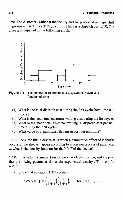
278 V Poisson Processes
time. The customers gather at the facility and are processed or dispatchedin groups at fixed times T, 2T, 3T, .... There is a dispatch cost of K. Theprocess is depicted in the following graph.
w0
E
0 TTime
2TE
Figure 1.1 The number of customers in a dispatching system as afunction of time.
(a) What is the total dispatch cost during the first cycle from time 0 totime Ti
(b) What is the mean total customer waiting cost during the first cycle?(c) What is the mean total customer waiting + dispatch cost per unit
time during the first cycle?(d) What value of T minimizes this mean cost per unit time?
1.11. Assume that a device fails when a cumulative effect of k shocksoccurs. If the shocks happen according to a Poisson process of parameterA, what is the density function for the life T of the device?
1.12. Consider the mixed Poisson process of Section 1.4, and supposethat the mixing parameter 0 has the exponential density f(O) = e-0 for0>0.
(a) Show that equation (1.3) becomes
Pr{X'(t)=j}=\1+t1J\l+t), forj=0,1,....

2. The Law of Rare Events 279
(b) Show that+ k I 1;+k+i
Pr{X'(t)=j,X'(t+s)=j+k} =I . )t's"(l +s+t/so that X'(t) and the increment X'(t + s) - X'(t) are not independent ran-dom variables, in contrast to the simple Poisson process as defined in Sec-tion 1.2.
2. The Law of Rare Events
The common occurrence of the Poisson distribution in nature is explainedby the law of rare events. Informally, this law asserts that where a certainevent may occur in any of a large number of possibilities, but where theprobability that the event does occur in any given possibility is small, thenthe total number of events that do happen should follow, approximately,the Poisson distribution.
A more formal statement in a particular instance follows. Consider alarge number N of independent Bernoulli trials where the probability p ofsuccess on each trial is small and constant from trial to trial. Let X,,,,, de-note the total number of successes in the N trials, where X,,.4, follows thebinomial distribution
Pr{X1,.,, = k} =k!(N - k)! p'(1 - p)'-" for k = 0, ... , N. (2.1)
Now let us consider the limiting case in which N - x and p -4 0 insuch a way that Np = µ > 0 where p is constant. It is a familiar fact (seeI, Section 3) that the distribution for X,,.,, becomes, in the limit, the Pois-son distribution
e-'`µ1.
Pr{X,A = k} =k!
for k = 0, 1, .... (2.2)
This form of the law of rare events is stated as a limit. In stochasticmodeling, the law is used to suggest circumstances under which onemight expect the Poisson distribution to prevail, at least approximately.For example, a large number of cars may pass through a given stretch ofhighway on any particular day. The probability that any specified car is inan accident is, we hope, small. Therefore, one might expect that the actual

280 V Poisson Processes
number of accidents on a given day along that stretch of highway wouldbe, at least approximately, Poisson distributed.
While we have formally stated this form of the law of rare events as amathematical limit, in older texts, (2.2) is often called "the Poisson ap-proximation" to the binomial, the idea being that when N is large and p issmall, the binomial probability (2.1) may be approximately evaluated bythe Poisson probability (2.2) with .t = Np. With today's computingpower, exact binomial probabilities are not difficult to obtain, so there islittle need to approximate them with Poisson probabilities. Such is not thecase if the problem is altered slightly by allowing the probability ofsuccess to vary from trial to trial. To examine this proposal in detail, letE,, EZ, ... be independent Bernoulli random variables, where
Pr {E; = 1) = p; and Pr {E; = 0) = I - pi,
and let S = E, + + E,,. When p, = P2 _ = p, then S,, has a bino-mial distribution, and the probability Pr{S = k} for some k = 0, 1.... iseasily computed. It is not so easily evaluated when the p's are unequal, thebinomial formula generalizing to
!i
Pr{S = k} = I(k' p)'(2.3)where I'"' denotes the sum over all 0, 1 valued x;'s such that x, + +x,, = k.
Fortunately, Poisson approximation may still prove accurate and allowthe computational challenges presented by equation (2.3) to be avoided.
Theorem 2.1 Let E, e2.... be independent Bernoulli random vari-ables, where
Pr{E; = 1} = p, and Pr{E; = 0} = I - p;,
and let S,, = E, + + E,,. The exact probabilities for S,,, determined using(2.3), and Poisson probabilities with µ = p, + + p differ by at most
Ae-
Pr (S,, = k} -µ
k!(2.4)
Not only does the inequality of Theorem 2.1 extend the law of rare eventsto the case of unequal p's, it also directly confronts the approximation

2. The Law of Rare Events 281
issue by providing a numerical measure of the approximation error. Thusthe Poisson distribution provides a good approximation to the exact prob-abilities whenever the pi's are uniformly small as measured by the rightside of (2.4). For instance, when p, = P2 = ... = µ/n, then the right sideof (2.4) reduces to µ2/n, which is small when n is large, and thus (2.4) pro-vides another means of obtaining the Poisson distribution (2.2) as a limitof the binomial probabilities (2.1).
We defer the proof of Theorem 2.1 to the end of this section, choosingto concentrate now on its implications. As an immediate consequence, forexample, in the context of the earlier car accident vignette, we see that theindividual cars need not all have the same accident probabilities in orderfor the Poisson approximation to apply.
2.1 The Law of Rare Events and the Poisson Process
Consider events occurring along the positive axis [0, oc) in the mannershown in Figure 2.1. Concrete examples of such processes are the timepoints of the x-ray emissions of a substance undergoing radioactive decay,the instances of telephone calls originating in a given locality, the occur-rence of accidents at a certain intersection, the location of faults or defectsalong the length of a fiber or filament, and the successive arrival times ofcustomers for service.
Let N((a, b]) denote the number of events that occur during the interval(a, b]. That is, if t, < t,-< t3 < denote the times (or locations, etc.) of
N((a, b]) = 3
ti t, a b t
Figure 2.1 A Poisson point process.

282 V Poisson Processes
successive events, then N((a, b]) is the number of values t; for whicha<t, b.
We make the following postulates:
(1) The numbers of events happening in disjoint intervals are indepen-dent random variables. That is, for every integer m = 2, 3, ... andtime points t0 = 0 < t, < t, < < t,,,, the random variables
N((to, ti]), N((t t,]), ... , N((t,,,-,, t])
are independent.(2) For any time t and positive number h, the probability distribution
of N((t, t + h]), the number of events occurring between time t andt + h, depends only on the interval length h and not on the time t.
(3) There is a positive constant A for which the probability of at leastone event happening in a time interval of length h is
Pr{N((t,t+ h]) ? 1) = Ah + o(h) ash 0.
(Conforming to a common notation, here o(h) as h .L 0 stands for ageneral and unspecified remainder term for which o(h)/h - 0 ash 10. That is, a remainder term of smaller order than h as h vanishes.)
(4) The probabilty of two or more events occurring in an interval oflength h is o(h), or
Pr{N((t, t + h]) ? 2} = o(h), h 10.
Postulate 3 is a specific formulation of the notion that events are rare.Postulate 4 is tantamount to excluding the possibility of the simultaneousoccurrence of two or more events. In the presence of Postulates 1 and 2,Postulates 3 and 4 are equivalent to the apparently weaker assumption thatevents occur singly and discretely, with only a finite number in any finiteinterval. In the concrete illustrations cited earlier, this requirement is usu-ally satisfied.
Disjoint intervals are independent by 1, and 2 asserts that the distribu-tion of N((s, t]) is the same as that of N((0, t - s]). Therefore, to describethe probability law of the system, it suffices to determine the probabilitydistribution of N((0, t]) for an arbitrary value of t. Let
Pk(t) = Pr{N((0, t]) = k}.

2. The Law of Rare Events 283
We will show that Postulates 1 through 4 require that Pk(t) be the Poisson
distribution(At)ke-Ar
Pk(t) = k! for k = 0, 1, .... (2.5)
To establish (2.5), divide the interval (0, t] into n subintervals of equallength h = t/n, and let
11 if there is at least one event in the interval ((i - 1)t/n, it/n],
0 otherwise.
Then S,, = E, + + E counts the total number of subintervals that con-tain at least one event, and
p, = Pr{E; = 1) = Atln + o(tin) (2.6)
according to Postulate 3. Upon applying (2.4), we see thatµ
WeµI <_ n[At/n + o(tln)]2Pr(S,, = k} -
k!
(n+211to(n) +no(nl,
n /
where'I
µ = p, = At + no(t/n). (2.7)
Because o(h) = o(t/n) is a term of order smaller than h = tin for large n,it follows that
n o(tln) = to(tln) = t o(h)
tin h
vanishes for arbitrarily large n. Passing to the limit as n - oo, then, we de-duce that
µke-lim Pr{S = k} =
k!, with µ = At.
To complete the demonstration, we need only show that
lim Pr{S = k} = Pr{N((0, t]) = k} = Pk(t).x

284 V Poisson Processes
But S,, differs from N((0, t]) only if at least one of the subintervals con-tains two or more events, and Postulate 4 precludes this because
IPk(t) - Pr{S = k}l Pr{N((0, t])
Pr(N(((i - 1)t it11 2l
r=i tl l n nil J
<_ n o(t/n) (by Postulate 4)
-3 0 as n - co.
By taking n arbitrarily large, or equivalently, by dividing the interval(0, t] into arbitrarily small subintervals, we see that it must be the case that
xe AlPr{N((0, t]) = k) =
(At)ki fork ? 0,
and Postulates 1-4 imply the Poisson distribution.Postulates 1 through 4 arise as physically plausible assumptions in
many circumstances of stochastic modeling. The postulates seem ratherweak. Surprisingly, they are sufficiently strong to force the Poisson be-havior just derived. This motivates the following definition.
Definition Let N((s, t]) be a random variable counting the number ofevents occurring in an interval (s, t]. Then N((s, t]) is a Poisson pointprocess of intensity A > 0 if
(i) for every m = 2, 3.... and distinct time points to = 0 < t, < t2 << t,,,, the random variables
N((to, t.l ), N((t,, t,]), ... , t,,,])
are independent; and(ii) for any times s < t the random variable N((s, t]) has the Poisson
distribution
Pr{N((s, t]) = k} =Wt - s)]ke a(Is)
ki k = 0,1,....
Poisson point processes often arise in a form where the time parameteris replaced by a suitable spatial parameter. The following formal exampleillustrates this vein of ideas. Consider an array of points distributed in a

2. The Law of Rare Events 285
space E (E is a Euclidean space of dimension d ? 1). Let N(A) denote thenumber of points (finite or infinite) contained in the region A of E. We pos-tulate that N(A) is a random variable. The collection {N(A)} of randomvariables, where A varies over all possible subsets of E, is said to be a ho-mogeneous Poisson process if the following assumptions are fulfilled:
(i) The numbers of points in nonoverlapping regions are independentrandom variables.
(ii) For any region A of finite volume, N(A) is Poisson distributed withmean AIAI, where IAI is the volume of A. The parameter A is fixedand measures in a sense the intensity component of the distribution,which is independent of the size or shape. Spatial Poissonprocesses arise in considering such phenomena as the distributionof stars or galaxies in space, the spatial distribution of plants andanimals, and the spatial distribution of bacteria on a slide. Theseideas and concepts will be further studied in Section 5.
2.2 Proof of Theorem 2.1
First, some notation. Let e(p) denote a Bernoulli random variable withsuccess probability p, and let X(O) be a Poisson distributed random vari-able with parameter 0. We are given probabilities p ... , p,, and letµ = p, + + p,,. With ( p 1 ), . . . , e(p,,) assumed to be independent, wehave S,, = e(p,) + + e(,,), and according to Theorem 1.1, we maywrite X(µ) as the sum of independent Poisson distributed random vari-ables in the form X(µ) = X(p,) + + X(,,). We are asked to comparePr{S = k} with Pr{X(µ) = k}, and, as a first step, we observe that if S,,and X(µ) are unequal, then at least one of the pairs e(pk) and X(pk) mustdiffer, whence
'I
lPr{S = k) - Pr{X(µ) = k}I < Pr{e(pJ X(pA)). (2.8)k=1
As the second step, observe that the quantities that are compared on theleft of (2.8) are the marginal distributions of S and X(µ), while the boundon the right is a joint probability. This leaves us free to choose the jointdistribution that makes our task the easiest. That is, we are free to specifythe joint distribution of each e(pp) and X(pk), as we please, provided onlythat the marginal distributions are Bernoulli and Poisson, respectively.

286 V Poisson Processes
To complete the proof, we need to show that Pr{e(p) 0 X(p) } <_ p2 forsome Bernoulli random variable E(p) and Poisson random variable X(p),since this reduces the right side of (2.8) to that of (2.4). Equivalently, wewant to show that 1 - p2 S Pr{E(p) = X(p) } = Pr{E(p) = X(p) = 01 +Pr{E(p) = X(p) = I), and we are free to choose the joint distribution, pro-vided that the marginal distributions are correct.
Let U be a random variable that is uniformly distributed over the inter-val (0, 1]. Define
E(p) =
1 if0<U5p,0
and for k = 0, l , ... , set
k-1
X(p) = k when'e-v
r=0 it<U<_
i=0
p'e-''i!
It is elementary to verify that e(p) and X(p) have the correct marginal dis-tributions. Furthermore, because 1 - p < e", we have E(p) = X(p) = 0only for U:5 1 - p, whence Pr{E(p) = X(p) = 0) = 1 - p. Similarly,E(p) = X(p) = 1 only when e -P < U <- (1 + p)e "', whence Pr{E(p) _X(p) = I) = pe ''. Upon summing these two evaluations, we obtain
Pr {E(p)=X(p)} = 1 - p+peP= 1 -p2as was to be shown. This completes the proof of (2.4).
Problem 2.10 calls for the reader to review the proof and to discover thesingle line that needs to be changed in order to establish the stronger result
/1
IPr{S in I) - Pr(X(µ) in I) I Yk=1
for any set of nonnegative integers I.
Exercises
2.1. Determine numerical values to three decimal places for Pr{X = k},k = 0, 1, 2, when
(a) X has a binomial distribution with parameters n = 20 and p = 0.06.(b) X has a binomial distribution with parameters n = 40 and p = 0.03.(c) X has a Poisson distribution with parameter A = 1.2.

problems 287
2.2. Explain in general terms why it might be plausible to assume thatthe following random variables follow a Poisson distribution:
(a) The number of customers that enter a store in a fixed time period.(b) The number of customers that enter a store and buy something in a
fixed time period.(c) The number of atomic particles in a radioactive mass that disinte-
grate in a fixed time period.
2.3. A large number of distinct pairs of socks are in a drawer, all mixedup. A small number of individual socks are removed. Explain in generalterms why it might be plausible to assume that the number of pairs amongthe socks removed might follow a Poisson distribution.
2.4. Suppose that a book of 600 pages contains a total of 240 typograph-ical errors. Develop a Poisson approximation for the probability that threeparticular successive pages are error-free.
Problems
2.1. Let X(n, p) have a binomial distribution with parameters n and p.Let n --> x and p - 0 in such a way that np = A. Show that
lim Pr{ X(n, p) = 01 = e'
and
Pr{X(n, p) = k + I) Afor k = 0, 1, ... .lim { ( p) = k} k + 1,I--- Pr X n,
2.2. Suppose that 100 tags, numbered 1 , 2, ... , 100, are placed into anurn, and 10 tags are drawn successively, with replacement. Let A be theevent that no tag is drawn twice. Show that
Pr(A) = (1 - ioo). (1 - iw)
Use the approximation
= 0.6282.
1 -x-e-` forx-0

288 V Poisson Processes
to get
Pr{A} - exp{-100 (1 + 2 + + 9)} = e°-45 = 0.6376.
Interpret this in terms of the law of rare events.
2.3. Suppose that N pairs of socks are sent to a laundry, where they arewashed and thoroughly mixed up to create a mass of unmatched socks.Then n socks are drawn at random without replacement from the pile. LetA be the event that no pair is among the n socks so selected. Show that
Pr{A} =
Use the approximation
to get
2"(n)
- ; (1 2N-il(2N)n
1-x-e-.Y forx- 0
Pr{A} = expi _ n(n-1)
2N-i} exp{4N '
the approximations holding when n is small relative to N, which is large.Evaluate the exact expression and each approximation when N = 100 andn = 10. Is the approximation here consistent with the actual number ofpairs of socks among the n socks drawn having a Poisson distribution?
Answer: Exact 0.7895; Approximate 0.7985.
2.4. Suppose that N points are uniformly distributed over the interval[0, N). Determine the probability distribution for the number of points inthe interval [0, 1) as N - c.
2.5. Suppose that N points are uniformly distributed over the surface ofa circular disk of radius r. Determine the probability distribution for thenumber of points within a distance of one of the origin as N -* co, r - co,N/(7rr2)_A.
2.6. Certain computer coding systems use randomization to assignmemory storage locations to account numbers. Suppose that N = MA dif-

Problems 289
ferent accounts are to be randomly located among M storage locations.Let X; be the number of accounts assigned to the ith location. If the ac-counts are distributed independently and each location is equally likely tobe chosen, show that Pr{X; = k} - e-"Ak/k! as N - oo. Show that X; andX; are independent random variables in the limit, for distinct locationsi j. In the limit, what fraction of storage locations have two or more ac-counts assigned to them?
2.7. N bacteria are spread independently with uniform distribution on amicroscope slide of area A. An arbitrary region having area a is selected forobservation. Determine the probability of k bacteria within the region ofarea a. Show that as N oc and a -3 0 such that (alA)N -3 c (0 < c < oo),then p(k) -3 e-`c'lk!.
2.8. Using (2.3), evaluate the exact probabilities for S,, and the Poissonapproximation and error bound in (2.4) when n = 4 and p, = 0.1, p2 = 0.2,p., = 0.3, and p4= 0.4.
2.9. Using (2.3), evaluate the exact probabilities for S,, and the Poissonapproximation and error bound in (2.4) when n = 4 and p, = 0.1, P2 = 0.1,p3=0.1,andp4=0.2.
2.10. Review the proof of Theorem 2.1 in Section 2.2 and establish thestronger result
Pr{S in 1 } - Pr{X(µ) in I }k=1
for any set of nonnegative integers I.
2.11. Let X and Y be jointly distributed random variables and B anarbitrary set. Fill in the details that justify the inequality JPr{X in B} -Pr{Yin B}1 Pr [X * Y}.
Hint: Begin with
{XinB} = {XinBandYinB) or {XinBand YnotinB}
C(Yin B} or {X/Y}.

290 V Poisson Processes
2.12. Computer Challenge Most computers have available a routinefor simulating a sequence U,,, U . . . of independent random variables,each uniformly distributed on the interval (0, 1). Plot, say, 10,000 pairs
on the unit square. Does the plot look like what you would ex-pect? Repeat the experiment several times. Do the points in a fixed num-ber of disjoint squares of area 1/10,000 look like independent unit Pois-son random variables?
'3. Distributions Associated with the Poisson Process
A Poisson point process N((s, t]) counts the number of events occurringin an interval (s, t]. A Poisson counting process, or more simply a Poissonprocess X(t), counts the number of events occurring up to time t. Formally,X(t) = N((0, t]).
Poisson events occurring in space can best be modeled as a pointprocess. For Poisson events occurring on the positive time axis, whetherwe view them as a Poisson point process or Poisson counting process islargely a matter of convenience, and we will freely do both. The two de-scriptions are equivalent for Poisson events occurring along a line. ThePoisson process is the more common and traditional description in thiscase because it allows a pictorial representation as an increasing integer-valued random function taking unit steps.
Figure 3.1 shows a typical sample path of a Poisson process where W isthe time of occurrence of the nth event, the so-called waiting time. It is oftenconvenient to set W, = 0. The differences S,, = W,,,, - W are called sojourntimes; S,, measures the duration that the Poisson process sojourns in state n.
X(t)
3
2
I
1 J
01 11 4-Wo WI W2 Wv
H- S o I S i Sz +{Figure 3.1 A typical sample path of a Poisson process showing the waiting
times W and the sojourn times S,,.

3. Distributions Associated with the Poisson Process 291
In this section we will determine a number of probability distributionsassociated with the Poisson process X(t), the waiting times W,,, and the so-journ times S.
Theorem 3.1 The waiting time W has the gamma distribution whoseprobability density function is
1
(n - 1)!e n = 1,2,...,t?0. (3.1)
In particular, W,, the time to the first event, is exponentially distributed:
Ae ", t ? 0. (3.2)
Proof The event W,, < t occurs if and only if there are at least n eventsin the interval (0, t], and since the number of events in (0, t] has a Poissondistribution with mean At we obtain the cumulative distribution functionof W via
F,,(t) = Pr{W : t} = Pr{X(t) ? n}
(At)ke"t
&k
=1-k!k=O
n= 1,2,...,t?0.
We obtain the probability density function by differentiating the cu-mulative distribution function. Then
d
d
I El
At (At)'- (At)"-111a--+ +...+Jrdt 1! 2! (n - 1)!
e "A +
A(At)+
A(At)'-
+ + A(At)"-2
1! 2! (n - 2)!
"11+
At (At)2 (At)"-1 1+Ae -+ J1! 2! (n - 1)!
e"`, n = 1, 2, . . . , t ?0.(n - 1)!

292 V Poisson Processes
There is an alternative derivation of the density in (3.1) that uses thePoisson point process N((s, t]) and proceeds directly without differentia-tion. The event t < W t + At corresponds exactly to n - 1 occurrencesin (0, t] and one in (t, t + At], as depicted in Figure 3.2.
N((O,t])=n- 1 N((t,t+At])= I
t t+At
W.
Figure 3.2
Then
Pr(t < W,,:!:-: t + At) + o(At) [see I, (2.5)]
= Pr{N((0, t]) = n - 1) Pr{N((t, t + At]) = 1) + o(At)(,kt),-yea,
A(At) + o(Ot).(n - 1)!
Dividing by At and passing to the limit as At 0 we obtain (3.2).Observe that Pr{N((t, t + At]) ? 1 } = Pr{N((t, t + At]) = 1 } + o(At) _
A(At) + o(Ot).
Theorem 3.2 The sojourn times So, S ... , are independent ran-dom variables, each having the exponential probability density function
A(s) _ Ae .', s ? 0. (3.3)
Proof We are being asked to show that the joint probability densityfunction of So, S ... , is the product of the exponential densitiesgiven by
si, ... , (Ae-x,,,_,). (3.4)
We give the proof only in the case n = 2, the general case being entirelysimilar. Referring to Figure 3.3 we see that the joint occurrence of
s, < S, < s, + As, and s, < S, < s, + Os2
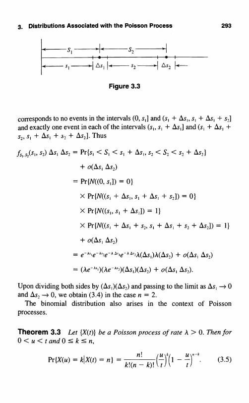
3. Distributions Associated with the Poisson Process 293
.0--- S1 <---- S,
F-- S1 - I s1 I< S2 -- LS?
Figure 3.3
corresponds to no events in the intervals (0, s,] and (s, + As,, s, + As, + s,]and exactly one event in each of the intervals (s s, + Os,] and (s, + As, +s s, + As, + s, + Os,]. Thus
fs,.s,(S,, s,) As, As, = Pr{s, < S, < s, + As,, s, < S, < s, + As,)
+ O(1s, Os,)
= Pr{N((0, s,]) = 0)
X Pr{N((s1 + As,, s, + As, + s,]) = 0)
X Pr{N((s1, s, + Os,]) = 1)
X Pr {N((s, + As, + s,, s, + As, + s, + Os,]) = 1 }
+ o(Ls, Os,)
= e-as,e-x.,,e-as.,,e A,,,,k(Os1)A(Os,) + o(Os, Os,)
= (Ae-A8)(Ae-A',)(Os1)(Os,) + o(Os, Os,).
Upon dividing both sides by (As1)(As,) and passing to the limit as As, ---> 0and As, - 0, we obtain (3.4) in the case n = 2.
The binomial distribution also arises in the context of Poissonprocesses.
Theorem 3.3 Let {X(t)} be a Poisson process of rate A > 0. Then for0<u<tand 0:k--:: n,
n! (ulkr u -kPr{X(u) = k X(t) = n) =
k!(n - k)! t 111 t) .(3.5)

294 V Poisson Processes
Proof Straightforward computations give
Pr{X(u) = klX(t) = n} =Pr{X(u) = k and X(t) = n }
Pr{X(t) = n)
which establishes (3.5).
Exercises
Pr{X(u) = k and X(t) - X(u) = n - k}Pr{X(t) = n}
{e-""(Au)Vk! } { e x(r_"'[A(t - u)]"-"/(n - k)!)
e "'(At)"/n!
n! u"(t -
k! (n - k)!
3.1. A radioactive source emits particles according to a Poisson processof rate A = 2 particles per minute. What is the probability that the first par-ticle appears after three minutes?
3.2. A radioactive source emits particles according to a Poisson processof rate A = 2 particles per minute.
(a) What is the probability that the first particle appears some timeafter three minutes but before five minutes?
(b) What is the probability that exactly one particle is emitted in the in-terval from three to five minutes?
3.3. Customers enter a store according to a Poisson process of rate A = 6per hour. Suppose it is known that but a single customer entered duringthe first hour. What is the conditional probability that this person enteredduring the first fifteen minutes?
3.4. Let X(t) be a Poisson process of rate 6 = 3 per hour. Find the con-ditional probability that there were two events in the first hour, given thatthere were five events in the first three hours.

Problems 295
3.5. Let X(t) be a Poisson process of rate 6 per hour. Find the conditionalprobability that there were m events in the first t hours, given that therewere n events in the first T hours. Assume 0 s m <_ n and 0 < t < T.
3.6. For i = 1, . . ., n, let {X;(t); t ? 0} be independent Poissonprocesses, each with the same parameter A. Find the distribution of thefirst time that at least one event has occurred in every process.
3.7. Customers arrive at a service facility according to a Poissonprocess of rate A customers/hour. Let X(t) be the number of customers thathave arrived up to time t. Let W W, . . . be the successive arrival timesof the customers. Determine the conditional mean E[WSIX(t) = 3].
3.8. Customers arrive at a service facility according to a Poissonprocess of rate A = 5 per hour. Given that 12 customers arrived during thefirst two hours of service, what is the conditional probability that 5 cus-tomers arrived during the first hour?
3.9. Let X(t) be a Poisson process of rate A. Determine the cumulativedistribution function of the gamma density as a sum of Poisson probabil-ities by first verifying and then using the identity W,. t if and only ifX(t) ? r.
Problems
3.1. Let X(t) be a Poisson process of rate A. Validate the identity
{W,>W,W,>w,}
if and only if
{X(w,) = 0, X(w,) - X(w,) = 0 or 1).
Use this to determine the joint upper tail probability
Pr{W, > w, W, > w,} = Pr{X(w1) = 0, X(w,) - X(w,) = 0 or 1 }
= A(w, - w )]e-Ao,,
Finally, differentiate twice to obtain the joint density function
f(w w,) = A2 exp{-Aw,} for 0 < w, < w,.

296 V Poisson Processes
3.2. The joint probability density function for the waiting times W, andW, is given by
f(w w,) = A2 exp{-,1w,} for 0 < w, < w,.
Determine the conditional probability density function for W given thatW, = w,. How does this result differ from that in Theorem 3.3 whenn = 2 and k = 1?
3.3. The joint probability density function for the waiting times W, andW, is given by
f(w,, w,) = A2 exp{-Aw,} for 0 < w, < w,.
Change variables according to
So=W, and S,=W-W,and determine the joint distribution of the first two sojourn times. Com-pare with Theorem 3.2.
3.4. The joint probability density function for the waiting times W, andW, is given by
f(w W,) = A2 exp{-Aw,} for 0 < w, < w,.
Determine the marginal density functions for W, and W2, and check yourwork by comparison with Theorem 3.1.
3.5. Let X(t) be a Poisson process with parameter A. Independently, letT be a random variable with the exponential density
fT(t) = Oe for t > 0.
Determine the probability mass function for X(T).
Hint: Use the law of total probability and I, (6.4). Alternatively, usethe results of I, Section 5.2.
3.6. Customers arrive at a holding facility at random according to aPoisson process having rate A. The facility processes in batches of size Q.That is, the first Q - 1 customers wait until the arrival of the Qth cus-tomer. Then all are passed simultaneously, and the process repeats. Ser-

4. The Uniform Distribution and Poisson Processes 297
vice times are instantaneous. Let N(t) be the number of customers in theholding facility at time t. Assume that N(0) = 0 and let T = min (t ? 0:N(t) = Q} be the first dispatch time. Show that E[T] = Q/A and E[ f
oN(t)
dt] = [1 + 2 + + (Q - 1)]/A = Q(Q - 1)/2A.
3.7. A critical component on a submarine has an operating lifetime thatis exponentially distributed with mean 0.50 years. As soon as a componentfails, it is replaced by a new one having statistically identical properties.What is the smallest number of spare components that the submarineshould stock if it is leaving for a one-year tour and wishes the probabilityof having an inoperable unit caused by failures exceeding the spare in-ventory to be less than 0.02?
3.8. Consider a Poisson process with parameter A. Given that X(t) = nevents occur in time t, find the density function for W the time of occur-rence of the rth event. Assume that r I n.
3.9. The following calculations arise in certain highly simplified mod-els of learning processes. Let X,(t) and X2(t) be independent Poissonprocesses having parameters A, and k,, respectively.
(a) What is the probability that XI(t) = 1 before X2(t) = 1?(b) What is the probability that X,(t) = 2 before X,(t) = 2?
3.10. Let (W,} be the sequence of waiting times in a Poisson processof intensity A = 1. Show that X = 2" defines a nonnegativemartingale.
4. The Uniform Distribution and Poisson Processes
The major result of this section, Theorem 4.1, provides an important toolfor computing certain functionals on a Poisson process. It asserts that,conditioned on a fixed total number of events in an interval, the locationsof those events are uniformly distributed in a certain way.
After a complete discussion of the theorem and its proof, its applicationin a wide range of problems will be given.
In order to completely understand the theorem, consider first the fol-lowing experiment. We begin with a line segment t units long and a fixed

298 V Poisson Processes
number n of darts and throw darts at the line segment in such a way thateach dart's position upon landing is uniformly distributed along the seg-ment, independent of the location of the other darts. Let U, be the positionof the first dart thrown, U, the position of the second, and so on up to U,,.The probability density function is the uniform density
1 for 0 :5 u -< t,.fU(u) = t
0 elsewhere.
Now let W, : W, < < W denote these same positions, not in the orderin which the darts were thrown, but instead in the order in which theyappear along the line. Figure 4.1 depicts a typical relation betweenU, U,,..., U and W,,W,..... W,,.
The joint probability density function for W, W..... W is
f,......1 (w...... w,,)=n!t-" for0<w, <w,<... < w,, <t. (4.1)
For example, to establish (4.1) in the case n = 2 we have
.fV,.w,(w,, w,) Ow, Ow,
=Pr{w, < W, <w, +Awl, w,< W,<_w,+sw,}
=Pr{w,< U,:w,+Awl, w,<U,<w,+Ow,}+Pr{w, < U,<_w, +Ow,,w,< U, mow,+Ow,}
w , , ,
=2( t X t
w)=2t -iw,Sw,.
Dividing by Awl IXw, and passing to the limit gives (4.1). When n = 2,there are two ways that U, and U, can be ordered; either U, is less. than U,,or U, is less than U,. In general there are n! arrangements of U,, ... , Uthat lead to the same ordered values W, 5 . :!5 W,,, thus giving (4.1).
1U, U U, U, U - ,1 .i0 W, W, W, W W t
Figure 4.1 W, W,, ..., W,, are the values U, U,, ..., U arranged inincreasing order.

4. The Uniform Distribution and Poisson Processes 299
Theorem 4.1 Let W, W,, . . . be the occurrence times in a Poissonprocess of rate A > 0. Conditioned on N(t) = n, the random variablesW, W,, ... , W have the joint probability density function
fV,.....w w) = n!t-n for O < w, < ... < w,, C t. (4.2)
Proof The event w; < W < w; + Ow; for i = 1, ... , n and N(t) = ncorresponds to no events occurring in any of the intervals (0, w,], (w, +Awl, w,], . . . , (w,, + (w + Ow,,, t], and exactly one event ineach of the intervals (w1, w, + Ow,], (w,, W, + pw,], . . . , (w,,, w +These intervals are disjoint, and
Pr{N((0, w,]) = 0, . . . , N((w,, + Awl,, t]) = 0}
= e A1[eACa]
= e A`[1 + o(max{Aw;})],
while
Pr{N((w1, w, + Awl]) = 1, . . . , N((w,,, w,, + 1}
= A(iw) . . . o(max{Ow;})].
Thus
fw,.....14, X(,)=(w,, ... ,Awl?
=Pr{w,<W,<w,+Ow......o(Ow, .. Awl,)
Pr{w;<W:5 w;+Iw;,i= 1,...,n,N(t)=n}Pr{N(t) = n}
+ o(Ow, ... Awl,)
e-Ark(Owl) ...[1 + o(max{Aw;})]
eA'(At)"/n!
= n!t-"(iw,) o(max{Aw;})].
Dividing both sides by (Ow,) ... and letting Awl -4 0, ..., Aw -4 0establishes (4.2).

300 V Poisson Processes
Theorem 4.1 has important applications in evaluating certain symmet-ric functionals on Poisson processes. Some sample instances follow.
Example Customers arrive at a facility according to a Poisson processof rate A. Each customer pays $1 on arrival, and it is desired to evaluatethe expected value of the total sum collected during the interval (0, t] dis-counted back to time 0. This quantity is given by
X(t)
M =Er
I ep`yk],
where f3 is the discount rate, W,, WZ, ... are the arrival times, and X(t) isthe total number of arrivals in (0, t]. The process is shown in Figure 4.2.
$1
e-awi
e-sW2
0 W, Wz W.
Figure 4.2 A dollar received at time WR. is discounted to a present value attime 0 of
We evaluate the mean total discounted sum M by conditioning onX(t) = n. Then
x rM = I EI > e l`iJX(t) = nJ Pr{X(t) = n}. (4.3)
n=1 k=1
Let U,, ... , U denote independent random variables that are uniformlydistributed in (0, t]. Because of the symmetry of the functional1% , exp{-/3W} and Theorem 4.1, we have

4. The Uniform Distribution and Poisson Processes
r ,r
ELI =E eQuA
k=1 k=1
= nE[e-, ""]
Substitution into (4.3) then gives
M t[1 - nPr{X(t)=n}= -lit [1
- eI`]E[X(t)l
301
Example Viewing a fixed mass of a certain radioactive material, sup-pose that alpha particles appear in time according to a Poisson process ofintensity A. Each particle exists for a random duration and is then annihi-lated. Suppose that the successive lifetimes Y,, Y,, . . . of distinct particlesare independent random variables having the common distribution func-tion G(y) = Pr{Yk <- y}. Let M(t) count the number of alpha particles ex-isting at time t. The process is depicted in Figure 4.3.
Y
-
,
Y,
0 W. W, W..._ . W. t
Figure 4.3 A particle created at time WA <- t still exists at time t if WA + YA ? t.

302 V Poisson Processes
We will use Theorem 4.1 to evaluate the probability distribution of M(t)under the condition that M(O) = 0.
Let X(t) be the number of particles created up to time t, by assumptiona Poisson process of intensity A. Observe that M(t) S X(t); the number ofexisting particles cannot exceed the number of particles created. Condi-tion on X(t) = n and let W...... W,, - t be the times of particle creation.Then particle k exists at time t if and only if Wk + Yk ? t. Let
1{Wk+Y?t} _II
0
if W1 +Yk?t,if W+Y<t.
Then 1(Wk + Yk ? t) = 1 if and only if the kth particle is alive at time t.Thus
Pr{M(t) = mIX(t) = n} = Pr{ 7 1{W + Yk. ? t} = mIX(t) = ni.k=1
Invoking Theorem 4.1 and the symmetry among particles, we have
Pr1{W +Yk?t} =mIX(t)=ntk=1
(4.4)
=Pr1{Uk+Y>-t)=mk=1
where U, U2, ... , U are independent and uniformly distributed on (0, t].The right-hand side of (4.4) is readily recognized as the binomial distrib-ution in which
lrp=Pr{Uk.+Yk?t} =- IPr{Yk?t-u}dut0
1r= t f [I - G(t - u)] du (4.5)0
I1
=rf [I - G(z)] dz.0
Thus, explicitly writing the binomial distribution, we have
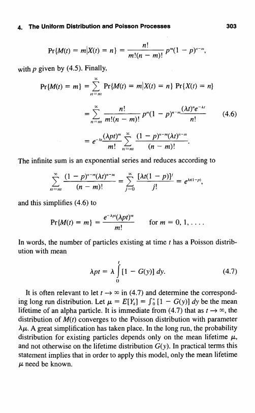
4, The Uniform Distribution and Poisson Processes 303
t
Pr{M(t) = mIX(t) = n} = m!(nn_ m)! p(1 - p)
with p given by (4.5). Finally,X
Pr{M(t) = m} = 7' Pr{M(t) = MIX(t) = n} Pr{X(t) = n}
- n!. f p(1 - p) (4.6)_,,, m!(n - m)! n!
A,
(Apt)"
m!
- p)°-,,,(At)
(n - m)!
The infinite sum is an exponential series and reduces according to
(1 -p)
,,,(At)
(n - m) ! l=0
[At(' - p)]' eARO -n,,
and this simplifies (4.6) to
Pr {M(t) = m} =e A"' (Apt)",
m!form = 0, 1. ... .
In words, the number of particles existing at time t has a Poisson distrib-ution with mean
r
Apt = A f [I - G(y)] dy. (4.7)0
It is often relevant to let t --> cc in (4.7) and determine the correspond-ing long run distribution. Let µ = E[Yk] = f,, [1 - G(y)] dy be the meanlifetime of an alpha particle. It is immediate from (4.7) that as t - x, thedistribution of M(t) converges to the Poisson distribution with parameterAA. A great simplification has taken place. In the long run, the probabilitydistribution for existing particles depends only on the mean lifetime µ,and not otherwise on the lifetime distribution G(y). In practical terms thisstatement implies that in order to apply this model, only the mean lifetimeµ need be known.

304 V Poisson Processes
4.1 Shot Noise
The shot noise process is a model for fluctuations in electrical currentsthat are due to chance arrivals of electrons to an anode. Variants of thephenomenon arise in physics and communication engineering. Assume:
(1) Electrons arrive at an anode according to a Poisson process(X(t); t ? 0) of constant rate A;
(2) An arriving electron produces a current whose intensity x timeunits after arrival is given by the impulse response function h(x).
The intensity of the current at time t is, then, the shot noiseX(t)
1(t) _ Y, h(t - Wk), (4.8)k=1
where W W, are the arrival times of the electrons.Common impulse response functions include triangles, rectangles, and
decaying exponentials of the form
h(x) = e x > 0,
where 0 > 0 is a parameter, and power law shot noise for which
h(x) = x °, for x > 0.
We will show that for a fixed time point t, the shot noise 1(t) has the sameprobability distribution as a certain random sum that we now describe. In-dependent of the Poisson process X(t), let U,, U,, . . . be independent ran-dom variables, each uniformly distributed over the interval (0, t], and de-fine Ek = h(Uk) for k = 1, 2, .... The claim is that 1(t) has the sameprobability distribution as the random sum
S(t) = E, + ... + EX(". (4.9)
With this result in hand, the mean, variance, and distribution of the shotnoise 1(t) may be readily obtained using the results on random sums de-veloped in II, Section 3. II, (3.9), for example, immediately gives us
E[I(t)] = E[S(t)] = AtE[h(U,)] = A f h(u) du0
and
Var[1(t)] = Jet{Var[h(U,)] + E[h(U,)]2)t
= At E[h(U,)Z] = A f h(u)2 du.

4, The Uniform Distribution and Poisson Processes 305
In order to establish that the shot noise 1(t) and the random sum S(t) sharethe same probability distribution, we need to show that Pr(I(t) <_ x) _Pr{S(t) : x} for a fixed t > 0. Begin with
X(t)
Pr{I(t) : x) = Pr{ I h(t - W) x}k=1
X(t)
_ Pr{ 7, h(t - W) < xl X(t) = n} Pr{X(t) = n)n=0 k=1
Pr{ 7, h(t - W) xI X(t) = n} Pr{X(t) = n},n =O k=1
and now invoking Theorem 4.1,
Pr h(t - Uk) !5 x{ Pr{X(t) = n}=n =O k =I
x rt l_ Pr{> h(Uk) x} Pr{X(t) = n}
n=0 k=1 J
(because Uk and t - Uk have the same distribution)
Pr{E1 +n=o
Pr(S(t)s x),
which completes the claim.
4.2. Sum Quota Sampling
A common procedure in statistical inference is to observe a fixed numbern of independent and identically distributed random variables X1, ..., Xand use their sample mean
X, + + XX _
n

306 V Poisson Processes
as an estimate of the population mean or expected value E[X,]. But sup-pose we are asked to advise an airline that wishes to estimate the failurerate in service of a particular component, or, what is nearly the same thing,to estimate the mean service life of the part. The airline monitors a newplane for two years and observes that the original component lasted 7months before failing. Its replacement lasted 5 months, and the third com-ponent lasted 9 months. No further failures were observed during the re-maining 3 months of the observation period. Is it correct to estimate themean life in service as the observed average (7 + 5 + 9)/3 = 7 months?
This airline scenario provides a realistic example of a situation in whichthe sample size is not fixed in advance but is determined by a preassignedquota t > 0. In sum quota sampling, a sequence of independent and iden-tically distributed nonnegative random variables X X,.... is observed se-quentially, the sampling continuing as long as the sum of the observationsis less than the quota t. Let this random sample size be denoted by N(t).Formally,
N(t)=max{n?0;X,+ + X,, <t}.
The sample mean is
W"( X, + +X,v<<, _N(t) - N(t)
Of course it is possible that X, ? t, and then N(t) = 0, and the samplemean is undefined. Thus, we must assume, or condition on, the event thatN(t) ? 1. An important question in statistical theory is whether or not thissample mean is unbiased. That is, how does the expected value of thissample mean relate to the expected value of, say, X,?
In general, the determination of the expected value of the sample meanunder sum quota sampling is very difficult. It can be carried out, however,in the special case in which the individual X summands are exponentiallydistributed with common parameter A, so that N(t) is a Poisson process.One hopes that the results in the special case will shed some light on thebehavior of the sample mean under other distributions.
The key is the use of Theorem 4.1 to evaluate the conditionalexpectation
E[W,, ';N(t) = n] = E[max{U ... , U,,)]
n ln + 11'

4. The Uniform Distribution and Poisson Processes 307
where U, ... , U are independent and uniformly distributed over theinterval (0, t]. Note also that
(At)"e"Pr{N(t) = nIN(t) > 0) =
n!(1 - e-")'
Then
E N(t)N(t) > 0] = > ELW'
nN(t) = nJ Pr{N(t) = nIN(t) > 0)
=t\( n )(I)j ( At)"e "`
n + 1nn!(1 - e-") J
1( lx (,kt)u+l
A \e"' 1 1),, (n + 1)
1l\e"'11/(e"'- 1 - At)
1 At
We can perhaps more clearly see the effect of the sum quota sampling ifwe express the preceding calculation in terms of the ratio of the bias to thetrue mean E[X,] = 1/A. We then have
E[X,] - At E[N(t)]
E[XI] - e"' _ 1 = ee1NUn - 1
The left side is the fraction of bias, and the right side expresses this frac-tion bias as a function of the expected sample size under sum quota sam-pling. The following table relates some values:
Fraction Bias E[N(t)]
0.58 1
0.31 2
0.16 3
0.17 40.03 5
0.015 6
0.0005 10

308 V Poisson Processes
In the airline example, we observed N(t) = 3 failures in the two-yearperiod, and upon consulting the above table, we might estimate the frac-tion bias to be something on the order of - 16%. Since we observedX,,,, = 7, a more accurate estimate of the mean time between failures(MTBF = E[X,]) might be 7/.84 = 8.33, an estimate that attempts to cor-rect, at least on average, for the bias due to the sampling method.
Looking once again at the table, we may conclude in general, that thebias due to sum quota sampling can be made acceptably small by choos-ing the quota t sufficiently large so that, on average, the sample size so se-lected is reasonably large. If the individual observations are exponentiallydistributed, the bias can be kept within 0.05% of the true value, providedthat the quota t is large enough to give an average sample size of 10 ormore.
Exercises
4.1. Let [X(t); t ? 0} be a Poisson process of rate A. Suppose it isknown that X(1) = n. For n = 1, 2, ... , determine the mean of the firstarrival time W,.
4.2. Let [X(t); t > 0) be a Poisson process of rate A. Suppose it isknown that X(1) = 2. Determine the mean of W, W,, the product of the firsttwo arrival times.
4.3. Customers arrive at a certain facility according to a Poisson processof rate A. Suppose that it is known that five customers arrived in the firsthour. Determine the mean total waiting time E[W, + W, + + WS].
4.4. Customers arrive at a service facility according to a Poissonprocess of intensity A. The service times Y,, Y,, . . . of the arriving cus-tomers are independent random variables having the common probabilitydistribution function G(y) = Pr{Yx < y}. Assume that there is no limit tothe number of customers that can be serviced simultaneously; i.e., there isan infinite number of servers available. Let M(t) count the number of cus-tomers in the system at time t. Argue that M(t) has a Poisson distributionwith mean Apt, where
p = t-' J[1 - G(y)] dy.0

Problems 309
4.5. Customers arrive at a certain facility according to a Poisson processof rate A. Suppose that it is known that five customers arrived in the firsthour. Each customer spends a time in the store that is a random variable,exponentially distributed with parameter a and independent of the othercustomer times, and then departs. What is the probability that the store isempty at the end of this first hour?
Problems
4.1. Let W, W2, ... be the event times in a Poisson process {X(t);t ? 0) of rate A. Suppose it is known that X(1) = n. For k < n, what is theconditional density function of W, ... , W _ W,,,,, ... , W,,, given thatW = w?
4.2. Let {N(t); t ? 0} be a Poisson process of rate A, representing the ar-rival process of customers entering a store. Each customer spends a dura-tion in the store that is a random variable with cumulative distributionfunction G. The customer durations are independent of each other and ofthe arrival process. Let X(t) denote the number of customers remaining inthe store at time t, and let Y(t) be the number of customers who have ar-rived and departed by time t. Determine the joint distribution of X(t) andY(t).
4.3. Let W,, W,, ... be the waiting times in a Poisson process {X(t);t ? 01 of rate A. Under the condition that X(1) = 3, determine the jointdistribution of U = W1IW, and V = (1 - W3)/(1 - W,).
4.4. Let W,, W, . . . be the waiting times in a Poisson process {X(t);t ? 0} of rate A. Independent of the process, let Z, ZZ, . . . be independentand identically distributed random variables with common probabilitydensity function f(x), 0 < x < oo. Determine Pr{Z > z1, where
Z=min {W,+Z,,W,+Z,,...}.
4.5. Let W,, W,, . . . be the waiting times in a Poisson process {N(t);t ? 0) of rate A. Determine the limiting distribution of W under the con-dition that N(t) = n as n -* - and t - oo in such a way that nit = (3 > 0.

310 V Poisson Processes
4.6. Customers arrive at a service facility according to a Poissonprocess of rate A customers/hour. Let X(t) be the number of customers thathave arrived up to time t. Let W, W,, . . . be the successive arrival timesof the customers.
(a) Determine the conditional mean E[W X(t) = 2].(b) Determine the conditional mean E[W, X(t) = 5].(c) Determine the conditional probability density function for W,,
given that X(t) = 5.
4.7. Let W W,, . . . be the event times in a Poisson process (X(t);t ? 0) of rate A, and letf(w) be an arbitrary function. Verify that
X(t) t
E[> .f(W )] = A Jf(w) dw.i=1 0
4.8. Electrical pulses with independent and identically distributedrandom amplitudes 6 62, . . . arrive at a detector at random times W,,W, ... according to a Poisson process of rate A. The detector output 0k(t)for the kth pulse at time t is
0k(t) =0 fort < Wk,
k exp{-a(t - W)} fort ? W.
That is, the amplitude impressed on the detector when the pulse arrives isek, and its effect thereafter decays exponentially at rate a. Assume that thedetector is additive, so that if N(t) pulses arrive during the time interval[0, t], then the output at time t is
N(t)
Z(t) _ 7 Ok(t).k=l
Determine the mean output E[Z(t)] assuming N(0) = 0. Assume that theamplitudes 4, 62, . . . are independent of the arrival times W,, W . ... .
4.9. Customers arrive at a service facility according to a Poisson processof rate k customers per hour. Let N(t) be the number of customers thathave arrived up to time t, and let W, , W,, . . . be the successive arrival timesof the customers. Determine the expected value of the product of the wait-ing times up to time t. (Assume that W, W, W,,,,, = 1 when N(t) = 0.)

5. Spatial Poisson Processes 311
4.10. Compare and contrast the example immediately following Theo-rem 4.1, the shot noise process of Section 4.1, and the model of Problem4.8. Can you formulate a general process of which these three examplesare special cases?
4.11. Computer Challenge Let U0, U,, . . . be independent randomvariables, each uniformly distributed on the interval (0, 1). Define a sto-chastic process {S,,} recursively by setting
So = 0 and for n > 0.
(This is an example of a discrete-time, continuous-state, Markov process.)When n becomes large, the distribution of S,, approaches that of a randomvariable S = SF, and S must have the same probability distribution asU(1 + S), where U and S are independent. We write this in the form
2b
S = U(1 + S),
from which it is easy to determine that E[S] = 1, Var[S] and even (theLaplace transform)
6 1 _E[e-oS] = exp (-J
e.,dull 0 > 0.
l 0+
The probability density functionf(s) satisfies
f(s) = 0 for s : 0, and
df= l f(s- 1), fors>0.
ds s
What is the 99th percentile of the distribution of S? (Note: Consider the shotnoise process of Section 4.1. When the Poisson process has rate A = I andthe impulse response function is the exponential h(x) = exp{-x}, then theshot noise 1(t) has, in the limit for large t, the same distribution as S.)
5. Spatial Poisson Processes
In this section we define some versions of multidimensional Poissonprocesses and describe some examples and applications.

312 V Poisson Processes
Let S be a set in n-dimensional space and let si be a family of subsetsof S. A point process in S is a stochastic process N(A) indexed by the setsA in , si and having the set of nonnegative integers (0, 1 , 2, ... ) as its pos-sible values. We think of "points" being scattered over S in some randommanner and of N(A) as counting the number of points in the set A. BecauseN(A) is a counting function, there are certain obvious requirements that itmust satifsy. For example, if A and B are disjoint sets in whose unionA U B is also in s4, then it must be that N(A U B) = N(A) + N(B). Inwords, the number of points in A or B equals the number of points in Aplus the number of points in B when A and B are disjoint.
The one-dimensional case, in which S is the positive half line and acomprises all intervals of the form A = (s, t], for 0 <- s < t, was intro-duced in Section 3. The straightforward generalization to the plane andthree-dimensional space that is now being discussed has relevance whenwe consider the spatial distribution of stars or galaxies in astronomy, ofplants or animals in ecology, of bacteria on a slide in medicine, and of de-fects on a surface or in a volume in reliability engineering.
Let S be a subset of the real line, two-dimensional plane, or three-dimensional space; let sl be the family of subsets of S and for any set Ain si; let IAI denote the size (length, area, or volume, respectively) of A.Then {N(A); A in sl} is a homogeneous Poisson point process of intensityA>0if
(i) for each A in A, the random variable N(A) has a Poisson distribu-tion with parameter AN;
(ii) for every finite collection {A...... of disjoint subsets of S, therandom variables N(A,), . . . , are independent.
In Section 2, the law of rare events was invoked to derive the Poissonprocess as a consequence of certain physically plausible postulates. Thisimplication serves to justify the Poisson process as a model in those situ-ations where the postualtes may be expected to hold. An analogous resultis available in the multidimensional case at hand. Given an arbitrary pointprocess {N(A); A in .si}, the required postulates are as follows:
(1) The possible values for N(A) are the nonnegative integers{0, 1, 2, ...} and 0 < Pr(N(A) = 0) < I if 0 < 1AJ < oo.

5. Spatial Poisson Processes 313
(2) The probability distribution of N(A) depends on the set A onlythrough its size (length, area, or volume) JAI, with the further prop-erty that Pr{N(A) ? 1 } = AJAJ + o(JAI) as JAI L 0.
(3) For m = 2, 3, . . . , if A,, A...... A. are disjoint regions, then N(A,),N(A,), . , N(A, UA2 U U A,,,) = N(AI) + N(A,) + + N(A,,,).
(4)
= 1lim
Pr{N(A) ? 1)A'o Pr{N(A) = 1}
The motivation and interpretation of these postulates is quite evident.Postulate 2 asserts that the probability distribution of N(A) does not de-pend on the shape or location of A, but only on its size. Postulate 3 re-quires that the outcome in one region not influence or be influenced by theoutcome in a second region that does not overlap the first. Postulate 4 pre-cludes the possibility of two points occupying the same location.
If a random point process N(A) defined with respect to subsets A ofEuclidean n-space satisfies Postulates 1 through 4, then N(A) is a homo-geneous Poisson point process of intensity A > 0, and
eAA(AIAI)k
Pr(N(A) = k} =kd
fork = 0, 1, ... . (5.1)
As in the one-dimensional case, homogeneous Poisson point processesin n-dimensions are highly amenable to analysis, and many results areknown for them. We elaborate a few of these consequences next, begin-ning with the uniform distribution of a single point. Consider a region Aof positive size JAI > 0, and suppose it is known that A contains exactlyone point; i.e., N(A) = 1. Where in A is this point located? We claim thatthe point is uniformly distributed in the sense that
Pr{N(B) = 1IN(A) = 1) = LB' for any set B C A. (5.2)
In words, the probability of the point being in any subset B of A is pro-portional to the size of B; that is, the point is uniformly distributed in A.The uniform distribution expressed in (5.2) is an immediate consequenceof elementary conditional probability manipulations. We write A = B U C,where B is an arbitrary subset of A and C is the portion of A not included

314 V Poisson Processes
in B. Then B and C are disjoint, so that N(B) and N(C) are independentPoisson random variables with respective means A BI and AICI. Then
Pr{N(B) = IIN(A) = 1 } =Pr{N(B) = 1, N(C) = 0}
r{ () - }
A'B1e-axe-Ac
AIAIe-A A
= IBI(because
AlI
Cj = A ),
and the proof is complete.The generalization to n points in a region A is stated as follows. Consider
a set A of positive size IAI > 0 and containing N(A) = n ? 1 points. Thenthese n points are independent and uniformly distributed in A in the sensethat for any disjoint partition A...... A,,, of A, where A, U U A,,, = A,and any positive integers k ... , k,,,, where k, + + k,,, = n, we have
Pr{N(A1= k...... N(A,,,) = k,,,
n!
k,! ... k,,,!
A,
A IAI
Equation (5.3) expresses the multinomial distribution for the conditionaldistribution of N(A,), . . . , N(A,,,) given that N(A) = n.
Example An Application in Astronomy Consider stars distributed inspace in accordance with a three-dimensional Poisson point process of in-tensity A > 0. Let x and y designate general three-dimensional, vectors,and assume that the light intensity exerted at x by a star located at y isf(x, y, a) = a/IIx - yII2 = al[(x, - y1)2 + (x, - y2)2 + (x3 - y3)2], wherea is a random parameter depending on the intensity of the star at y. We as-sume that the intensities a associated with different stars are independent,identically distributed random variables possessing a common mean µand variance o<;. We also assume that the combined intensity exerted at thepoint x due to light created by different stars accumulates additively. LetZ(x, A) denote the total light intensity at the point x due to signals ema-nating from all sources located in region A. Then
N(A) = n } (5.3)
JA J

Exercises 315
N(A)
Z(x, A) _ f(x, y,., a)
N(A)(5.4)
where y, is the location of the rth star in A. We recognize (5.4) as a ran-dom sum, as discussed in II, Section 3.2. Accordingly, we have the meanintensity at x given by
E[Z(x, A)] = (E[N(A)])(E[ f(x, y, a)]). (5.5)
Note that E[N(A)] = .1JAJ, while because we have assumed a and y to beindependent,
E[f(x, y, a)] = E[a]E[II x -
But as a consequence of the Poisson distribution of stars in space, we maytake y to be uniformly distributed in A. Thus
E[Ijx -JA 1
1 J xA
With µa = E[a], then (5.5) reduces to
E[Z(x, A)] = ' Pa J dy
A x -
Exercises
5.1. Bacteria are distributed throughout a volume of liquid according toa Poisson process of intensity 0 = 0.6 organisms per mm'. A measuringdevice counts the number of bacteria in a 10 mm' volume of the liquid.What is the probability that more than two bacteria are in this measuredvolume?
5.2. Customer arrivals at a certain service facility follow a Poissonprocess of unknown rate. Suppose it is known that 12 customers have ar-rived during the first three hours. Let Ni be the number of customers whoarrive during the ith hour, i = 1, 2, 3. Determine the probability thatN, = 3, N, = 4, and N; = 5.

316 V Poisson Processes
5.3. Defects (air bubbles, contaminants, chips) occur over the surface ofa varnished tabletop according to a Poisson process at a mean rate of onedefect per top. If two inspectors each check separate halves of a giventable, what is the probability that both inspectors find defects?
Problems
5.1. A piece of a fibrous composite material is sliced across its circularcross section of radius R, revealing fiber ends distributed across the circu-lar area according to a Poisson process of rate 100 fibers per cross section.The locations of the fibers are measured, and the radial distance of eachfiber from the center of the circle is computed. What is the probabilitydensity function of this radial distance X for a randomly chosen fiber?
5.2. Points are placed on the surface of a circular disk of radius one ac-cording to the following scheme. First, a Poisson distributed random vari-able N is observed. If N = n, then n random variables 0...... 0,, are in-dependently generated, each uniformly distributed over the interval[0, 2ir), and n random variables R . . . , R,, are independently generated,each with the triangular density f(r) = 2r, 0 < r < 1. Finally, the pointsare located at the positions with polar coordinates (R;, 9;), i = 1, . . . , n.What is the distribution of the resulting point process on the disk?
5.3. Let {N(A); A E R2) be a homogeneous Poisson point process in theplane, where the intensity is A. Divide the (0, t] X (0, t] square into n2boxes of side length d = t/n. Suppose there is a reaction between two ormore points whenever they are located within the same box. Determinethe distribution for the number of reactions, valid in the limit as t 7 00andd-*0insuch awaythat td- > 0.
5.4. Consider spheres in three-dimensional space with centers distrib-uted according to a Poisson distribution with parameter AIAJ, where CAInow represents the volume of the set A. If the radii of all spheres are dis-tributed according to F(r) with densityf(r) and finite third moment, showthat the number of spheres that cover a point t is a Poisson random vari-able with parameter ;Air f o r'f(r) dr.

problems 317
5.5. Consider a two-dimensional Poisson process of particles in theplane with intensity parameter v. Determine the distribution Fo(x) of thedistance between a particle and its nearest neighbor. Compute the meandistance.
5.6. Suppose that stars are distributed in space following a Poissonpoint process of intensity A. Fix a star alpha and let R be the distance fromalpha to its nearest neighbor. Show that R has the probability densityfunction
4A 7rx'fR(x) _ (4A7rx'-) expj 1, x > 0.
5.7. Consider a collection of circles in the plane whose centers are dis-tributed according to a spatial Poisson process with parameter AJAI, whereJ denotes the area of the set A. (In particular, the number of centers (A)in the set A follows the distribution law Pr(e(A) = k} = e AA[(A[AJ)'1k!].)The radius of each circle is assumed to be a random variable independentof the location of the center of the circle, with density functionf(r) and fi-nite second moment.
(a) Show that C(r), defined to be the number of circles that cover theorigin and have centers at a distance less than r from the origin, de-termines a variable-time Poisson process, where the time variableis now taken to be the distance r.
Hint: Prove that an event occurring between r and r + dr (i.e., there isa circle that covers the origin and whose center is in the ring of radius rto r + dr) has probability A27rr dr f ;f(p) dp + o(dr), and events occur-ring over disjoint intervals constitute independent r.v.'s. Show that C(r)is a variable-time (nonhomogeneous) Poisson process with parameter
x
A(r) = 27rAr f f (p) d p.
(b) Show that the number of circles that cover the origin is a Poissonrandom variable with parameter A f o 7rr2f(r) dr.

318 V Poisson Processes
6. Compound and Marked Poisson Processes
Given a Poisson process X(t) of rate A > 0, suppose that each event hasassociated with it a random variable, possibly representing a value or acost. Examples will appear shortly. The successive values Y Y,, ... areassumed to be independent, independent of the Poisson process, and ran-dom variables sharing the common distribution function
G(y) = Pr{Yk <_ y}.
A compound Poisson process is the cumulative value process defined byX(t)
Z(t) = 7 Y for t ? 0. (6.1)k=I
A marked Poisson process is the sequence of pairs (W, Y,), (W,, Y,), ...,where W,, W,, ... are the waiting times or event times in the Poissonprocess X(t).
Both compound Poisson and marked Poisson processes appear often asmodels of physical phenomena.
6.1. Compound Poisson Processes
Consider the compound Poisson process Z(t) 111; Yk. If A > 0 is the ratefor the process X(t) and µ = E[Y] and v2 = Var[Y,] are the common meanand variance for Y,, Y,, ... , then the moments of Z(t) can be determinedfrom the random sums formulas of II, Section 3.2 and are
E[Z(t)] = Apt; Var[Z(t)] = A(v'- + µ-)t. (6.2)
Examples(a) Risk Theory Suppose claims arrive at an insurance company in
accordance with a Poisson process having rate A. Let Yk be the magnitudeof the kth claim. Then Z(t) _ 110", Yk represents the cumulative amountclaimed up to time t.
(b) Stock Prices Suppose that transactions in a certain stock takeplace according to a Poisson process of rate A. Let Yk denote the change inmarket price of the stock between the kth and (k - 1)st transaction.
The random walk hypothesis asserts that Y, Y,, . . . are independent ran-dom variables. The random walk hypothesis, which has a history dating
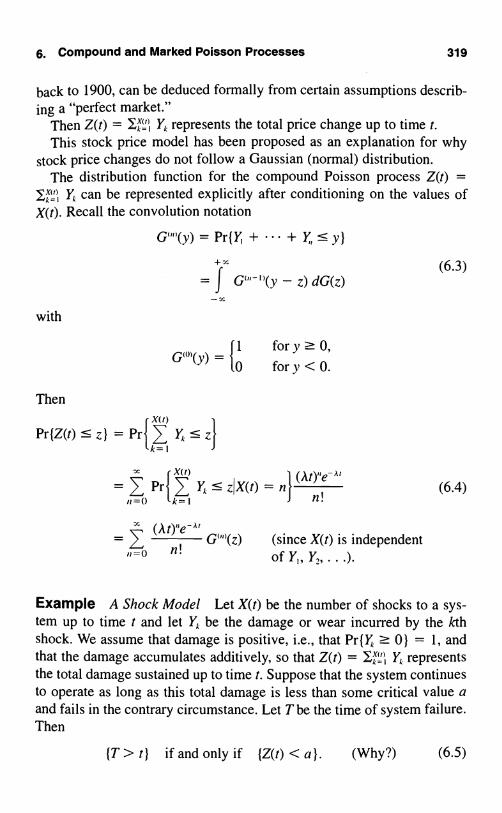
6. Compound and Marked Poisson Processes 319
back to 1900, can be deduced formally from certain assumptions describ-ing a "perfect market."
Then Z(t) _ IA=I'I,, Y, represents the total price change up to time t.This stock price model has been proposed as an explanation for why
stock price changes do not follow a Gaussian (normal) distribution.The distribution function for the compound Poisson process Z(t) _
IM11,, can be represented explicitly after conditioning on the values ofX(t). Recall the convolution notation
G"(y)=Pr{Y,+...+Y<_y}+f
J G")(y - z) dG(z)
with
Then
=o
-x
{1
0
for y ? 0,for y < 0.
r X(r)
Pr(Z(t) z} = Prj 2 Y < z}k=I
x(n ( 1 t)' - A ,
_ Pr 7, Y zjX(t) = n l/l
n=o k=1 n!
J
n! of
(6.3)
(6.4)
Example A Shock Model Let X(t) be the number of shocks to a sys-tem up to time t and let Yk be the damage or wear incurred by the kthshock. We assume that damage is positive, i.e., that Pr{Y. ? 0} = 1, andthat the damage accumulates additively, so that Z(t) = 111', Y, representsthe total damage sustained up to time t. Suppose that the system continuesto operate as long as this total damage is less than some critical value aand fails in the contrary circumstance. Let The the time of system failure.Then
G(01(y) =
(At)ne-At_ GOO (Z) (since X(t) is independent
{T > t} if and only if {Z(t) < a}. (Why?) (6.5)

320 V Poisson Processes
In view of (6.4) and (6.5), we havex
(At)"e-A,
Pr[T > t} = G("'(a).n=0 n!
All summands are nonnegative, so we may interchange integration andsummation to get the mean system failure time
x
E[T] = f Pr[T> t} dt0
x
G",,(a).
=0
This expression simplifies greatly in the special case in which Y Y2, .. .are each exponentially distributed according to the density gy(y) = µe F"for y > 0. Then the sum Y, + + Y has the gamma distribution
and
k=0
(µz)ke ,<<
_(pz)ke "<
k! k=n k!
x x x
7 G'(a)=7, Yn=0 n=0k=n
IM)keµa
k!
(Fa)ke-µa
k!
x(I-)ke_µa(1 + k)
k=0ki
= 1 + µa.
When Y, Y,, ... are exponentially distributed, then
E[T]= 1+µaA

6. Compound and Marked Poisson Processes 321
6.2. Marked Poisson Processes
Again suppose that a random variable Y is associated with the kth event in aPoisson process of rate A. W e stipulate that Y Y,, ... are independent, inde-pendent of the Poisson process, and share the common distribution function
G(y) = Pr{Y" : y}.
The sequence of pairs (W, Y,), (W,, Y,), ... is called a marked Poissonprocess.
We begin the analysis of marked Poisson processes with one of the sim-plest cases. For a fixed value p (0 < p < 1) suppose
Pr{Y"= 1} = p, Pr(Y"=0) = q = 1 -p.Now consider separately the processes of points marked with ones and ofpoints marked with zeros. In this case we can define the relevant Poissonprocesses explicitly by
X. (t) =k=1
Y and X0(t) = X(t) - X,(t).
Then nonoverlapping increments in X,(t) are independent random vari-ables, X,(0) = 0, and finally, Theorem 1.2 applies to assert that X,(t) has aPoisson distribution with mean Apt. In summary, X,(t) is a Poisson processwith rate Ap, and the parallel argument shows that X0(t) is a Poissonprocess with rate A(1 - p). What is even more interesting and surprisingis that X0(t) and X,(t) are independent processes! The relevant property tocheck is that Pr{X0(t) = j and X,(t) = k) = Pr{X0(t) = j) X Pr{X1(t) = k}for j, k = 0, 1, .... We establish this independence by writing
Pr{X0(t) = j, X,(t) = k} = Pr{X0(t) = j + k, XI(t) = k}
= Pr{X1(t) = kIX(t) = j + k} Pr{X(t) = j + k)
k-
J
j!k!p ( P) (j + k)!
[e-Ar(Apt)kI[e
A('-n"(A(1 - p)t)'Ik! j!
= Pr{X1(t) = k} Pr{X0(t) = j}
forj, k = 0, 1,....
(At)f+"e-A7(j + k)!

322 V Poisson Processes
Example Customers enter a store according to a Poisson process of rateA = 10 per hour. Independently, each customer buys something with prob-ability p = 0.3 and leaves without making a purchase with probability q =1 - p = 0.7. What is the probability that during the first hour 9 peopleenter the store and that 3 of these people make a purchase and 6 do not?
Let X, = X,(1) be the number of customers who make a purchase dur-ing the first hour and X0 = X(,(1) be the number of people who do not. ThenX, and Xo are independent Poisson random variables having respectiverates 0.3(10) = 3 and 0.7(10) = 7. According to the Poisson distribution,
3'e 3Pr{X, = 3) =
3!= 0.2240,
lee-7
= 14900Pr {X = 6) =6 !
,.
and
Pr{X1 = 3, X0 = 6} = Pr{X1 = 3) Pr{X = 61 = (0.2240)(0.1490) = 0.0334.
In our study of marked Poisson processes, let us next consider the casewhere the value random variables Y,, Y,, ... are discrete, with possible val-ues 0, 1, 2, ... and
Pr{Y = k} = ax > 0 for k = 0, 1, ... ,with Lak = 1.
In Figure 6.1, the original Poisson event times W, k, ... are shown on
Y, = 3
I
Y,=2
W, W, W, W4
Figure 6.1 A marked Poisson process. W, W,, . . . are the event times ina Poisson process of rate A. The random variables Y, Y,, . . . arethe markings, assumed to be independent and identically distrib-uted, and independent of the Poisson process.

6. Compound and Marked Poisson Processes 323
the bottom axis. Then a point is placed in the (t, y) plane at (W,,, Y,,) forevery n. For every integer k = 0, 1, 2.... one obtains a point process thatcorresponds to the times W for which Y = k. The same reasoning as inthe zero-one case applies to imply that each of these processes is Poisson,the rate for the kth process being Aak, and that processes for distinct val-ues of k are independent.
To state the corresponding decomposition result when the valuesY Y,, . . . are continuous random variables requires a higher level of so-phistication, although the underlying ideas are basically the same. To setthe stage for the formal statement, we first define what we mean by a non-homogeneous Poisson point process in the plane, thus extending the ho-mogeneous processes of the previous section. Let 0 = 0(x, y) be a non-negative function defined on a region S in the (x, y) plane. For each subsetA of S, let µ(A) = f fA 6(x, y) dx dy be the volume under 9(x, y) enclosedby A. A nonhomogeneous Poisson point process of intensity function0(x, y) is a point process {N(A); A C S) for which
(i) for each subset A of S, the random variable N(A) has a Poisson dis-tribution with mean µ(A);
(ii) for disjoint subsets A,, . . ., A,,, of S, the random variables N(A,), ... ,N(A,,,) are independent.
It is easily seen that the homogeneous Poisson point process of inten-sity A corresponds to the function 9(x, y) being constant, and 6(x, y) = Afor all x, y.
With this definition in hand, we state the appropriate decomposition re-sult for general marked Poisson processes.
Theorem 6.1 Let (W Y,), (W,, Y,), ... be a marked Poisson processwhere W W,, . are the waiting times in a Poisson process of rate Aand Y Y,, ... are independent identically distributed continuous randomvariables having probability density function g(y). Then (W Y),(W,, Y2), . . . form a two-dimensional nonhomogeneous Poisson pointprocess in the (t, y) plane, where the mean number of points in a region Ais given by
µ(A) = JJAg(y)dydt. (6.6)A

324 V Poisson Processes
Figure 6.2 diagrams the scene.
Y
o- o- 6 0
W, W3 W4 W5
Figure 6.2 A marked Poisson process.
Theorem 6.1 asserts that the numbers of points in disjoint intervals areindependent random variables. For example, the waiting times correspond-ing to positive values Y Y,, . . . form a Poisson process, as do the times as-sociated with negative values, and these two processes are independent.
Example Crack Failure The following model is proposed to describethe failure time of a sheet or volume of material subjected to a constantstress o. The failure time is viewed in two parts, crack initiation and crackpropagation.
Crack initiation occurs according to a Poisson process whose rate perunit time and unit volume is a constant A > 0 depending on the stresslevel a-. Crack initiation per unit time then is a Poisson process of rateA,IVJ, where IVI is the volume of material under consideration. We letW W,, . . . be the times of crack initiation.
Once begun, a crack grows at a random rate until it reaches a criticalsize, at which instant structural failure occurs. Let Yk be the time to reachcritical size for the kth crack. The cumulative distribution functionG, (y) = Pr{Yk s y} depends on the constant stress level a-.
We assume that crack initiations are sufficiently sparse as to makeY Y,, . . . independent random variables. That is, we do not allow twosmall cracks to join and form a larger one.
The structural failure time Z is the smallest of W, + Y,, W, + Y,..... Itis not necessarily the case that the first crack to appear will cause systemfailure. A later crack may grow to critical size faster.

6. Compound and Marked Poisson Processes 325
Figure 6.3 A crack failure model.
In the (t, y) plane, the event {min { Wk + Y,.) > z) corresponds to nopoints falling in the triangle A = ((t, y): t + y z, t ? 0, y ? 0), as shownin Figure 6.3.
The number of points N(O) falling in the triangle A has a Poisson dis-tribution with mean µ(0) given, according to (6.6), by
µ(A) = JJAIVjds g?(u) du
.s
= f AoIVI g,(u) du ds0
=AvIVI f Go(z - s)ds0
Z
= A,1VI f GQ(v) dv.0
From this we obtain the cumulative distribution function for structuralfailure time,
Pr(Z<-z) = I -Pr{Z>z} = 1 -Pr(N(L)=0}
= 1 - exp -,QV1 f GQ(v) dv .
0
Observe the appearance of the so-called size effect in the model,wherein the structure volume IVI affects the structural failure time even at
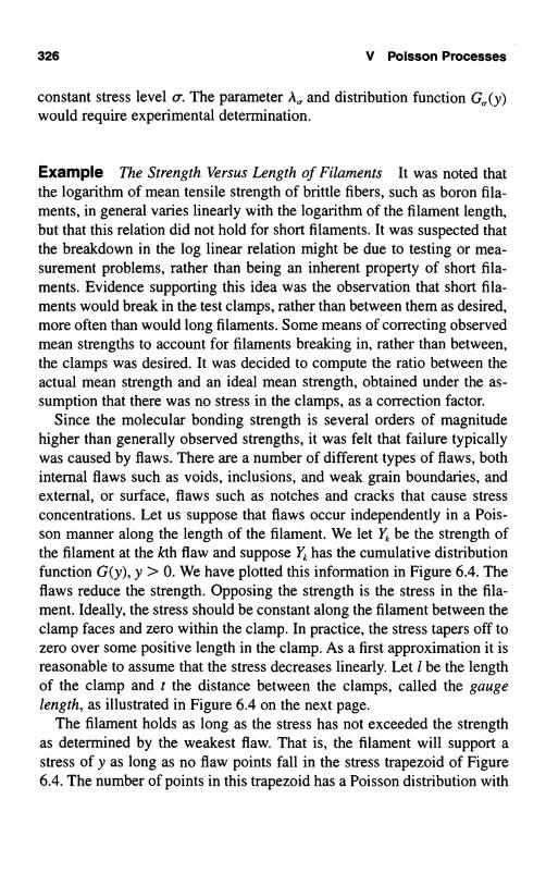
326 V Poisson Processes
constant stress level The parameter A and distribution function G,,(y)would require experimental determination.
Example The Strength Versus Length of Filaments It was noted thatthe logarithm of mean tensile strength of brittle fibers, such as boron fila-ments, in general varies linearly with the logarithm of the filament length,but that this relation did not hold for short filaments. It was suspected thatthe breakdown in the log linear relation might be due to testing or mea-surement problems, rather than being an inherent property of short fila-ments. Evidence supporting this idea was the observation that short fila-ments would break in the test clamps, rather than between them as desired,more often than would long filaments. Some means of correcting observedmean strengths to account for filaments breaking in, rather than between,the clamps was desired. It was decided to compute the ratio between theactual mean strength and an ideal mean strength, obtained under the as-sumption that there was no stress in the clamps, as a correction factor.
Since the molecular bonding strength is several orders of magnitudehigher than generally observed strengths, it was felt that failure typicallywas caused by flaws. There are a number of different types of flaws, bothinternal flaws such as voids, inclusions, and weak grain boundaries, andexternal, or surface, flaws such as notches and cracks that cause stressconcentrations. Let us suppose that flaws occur independently in a Pois-son manner along the length of the filament. We let Yk be the strength ofthe filament at the kth flaw and suppose Yk has the cumulative distributionfunction G(y), y > 0. We have plotted this information in Figure 6.4. Theflaws reduce the strength. Opposing the strength is the stress in the fila-ment. Ideally, the stress should be constant along the filament between theclamp faces and zero within the clamp. In practice, the stress tapers off tozero over some positive length in the clamp. As a first approximation it isreasonable to assume that the stress decreases linearly. Let l be the lengthof the clamp and t the distance between the clamps, called the gaugelength, as illustrated in Figure 6.4 on the next page.
The filament holds as long as the stress has not exceeded the strengthas determined by the weakest flaw. That is, the filament will support astress of y as long as no flaw points fall in the stress trapezoid of Figure6.4. The number of points in this trapezoid has a Poisson distribution with

6. Compound and Marked Poisson Processes 327
y*
A
kthflawDistance along filament
-H l 1-
Filament
B
Ideal stress
Actual' stress
Clamp
Figure 6.4 The stress versus strength of a filament under tension. Flaws re-ducing the strength of a filament below its theoretical maximumy* are distributed randomly along its length. The stress in the fila-ment is constant at the level y between clamps and tapers off tozero within the clamps. The filament fails if at any point along itslength a flaw reduces its strength below its stress.
mean µ(B) + 2µ(A). In particular, no points fall there with probabilitye-I"(B)+'a`A)1. If we let S be the strength of the filament, then
Pr(S > y) = e-?µ(A)-µ mf)
We compute
and
l= G(l
lAdx/t(A)
f
µ(B) = AtG(y).
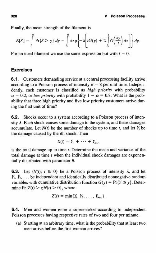
328 V Poisson Processes
Finally, the mean strength of the filament isx x
E[S] = J Pr{S > y} dy = J exp -A tG(y) + 2 JG() dx dy.0
For an ideal filament we use the same expression but with 1 = 0.
Exercises
6.1. Customers demanding service at a central processing facility arriveaccording to a Poisson process of intensity 6 = 8 per unit time. Indepen-dently, each customer is classified as high priority with probabilitya = 0.2, or low priority with probability 1 - a = 0.8. What is the prob-ability that three high priority and five low priority customers arrive dur-ing the first unit of time?
6.2. Shocks occur to a system according to a Poisson process of inten-sity A. Each shock causes some damage to the system, and these damagesaccumulate. Let N(t) be the number of shocks up to time t, and let Y bethe damage caused by the ith shock. Then
is the total damage up to time t. Determine the mean and variance of thetotal damage at time t when the individual shock damages are exponen-tially distributed with parameter 0.
6.3. Let {N(t); t ? 01 be a Poisson process of intensity A, and letY,, YZ, ... be independent and identically distributed nonnegative randomvariables with cumulative distribution function G(y) = Pr{Y <_ y}. Deter-mine Pr{Z(t) > zjN(t) > 0}, where
Z(t) = min{Y Y,, ... , YN,,,}
6.4. Men and women enter a supermarket according to independentPoisson processes having respective rates of two and four per minute.
(a) Starting at an arbitrary time, what is the probability that at least twomen arrive before the first woman arrives?

Problems 329
(b) What is the probability that at least two men arrive before the thirdwoman arrives?
6.5. Alpha particles are emitted from a fixed mass of material accordingto a Poisson process of rate A. Each particle exists for a random durationand is then annihilated. Suppose that the successive lifetimes Y Y,, . . . ofdistinct particles are independent random variables having the commondistribution function G(y) = Pr{Yk s y}. Let M(t) be the number of parti-cles existing at time t. By considering the lifetimes as markings, identifythe region in the lifetime, arrival-time space that corresponds to M(t), andthereby deduce the probability distribution of M(t).
Problems
6.1. Suppose that points are distributed over the half line [0, 00) accord-ing to a Poisson process of rate A. A sequence of independent and identi-cally distributed nonnegative random variables Y Y2, . . . is used to repo-sition the points so that a point formerly at location WA is moved to thelocation Wk + Yk. Completely describe the distribution of the relocatedpoints.
6.2. Suppose that particles are distributed on the surface of a circular re-gion according to a spatial Poisson process of intensity A particles per unitarea. The polar coordinates of each point are determined, and each angu-lar coordinate is shifted by a random amount, the amounts shifted for dis-tinct points being independent random variables following a fixed proba-bility distribution. Show that at the end of the point movement process,the points are still Poisson distributed over the region.
6.3. Shocks occur to a system according to a Poisson process of inten-sity A. Each shock causes some damage to the system, and these damagesaccumulate. Let N(t) be the number of shocks up to time t, and let Y; bethe damage caused by the ith shock. Then
X(t)=Y,+...+YN(,)
is the total damage up to time t. Suppose that the system continues to op-erate as long as the total damage is strictly less than some critical value a,and fails in the contrary circumstance. Determine the mean time to system

330 V Poisson Processes
failure when the individual damages Y have a geometric distribution withPr{Y= k} = p(1 - p)k,k= 0, 1,....
6.4. Let {X(t); t ? 0} and {Y(t); t ? 0} be independent Poissonprocesses with respective parameters A and µ. For a fixed integer a, letT = min { t ? 0; Y(t) = a) be the random time that the Y process firstreaches the value a. Determine k} for k = 0, 1, ... .
Hint: First consider = X(T,) in the case in which a = 1. Then hasa geometric distribution. Then argue that X(T,) for general a has thesame distribution as the sum of a independent 's and hence has a neg-ative binomial distribution.
6.5. Let (X(t); t ? 0) and (Y(t); t ? 0) be independent Poissonprocesses with respective parameters A and µ. Let T = min { t ? 0;Y(t) = I) be the random time of the first event in the Y process. DeterminePr{X(T/2) = k) fork = 0, 1.... .
6.6 Let W,, W,, . . . be the event times in a Poisson process {X(t); t ? 0}of rate A. A new point process is created as follows: Each point WA is re-placed by two new points located at W,, + Xk and Wk + YA, where X, Y,X,, Y,, . . . are independent and identically distributed nonnegative randomvariables, independent of the Poisson process. Describe the distribution ofthe resulting point process.
6.7. Let {N(t); t ? 01 be a Poisson process of intensity A, and letY Y,, . . . be independent and identically distributed nonnegative randomvariables with cumulative distribution function
G(y) = y° for 0 < y < 1.
Determine Pr{Z(t) > zIN(t) > 0), where
Z(t) = min{Y,,
Describe the behavior for large t.
6.8. Let {N(t); t ? 0) be a nonhomogeneous Poisson process of inten-sity A(t), t > 0, and let Y Y,, . . . be independent and identically distrib-uted nonnegative random variables with cumulative distribution function
G(y)=y" for0<y<1.

problems 331
Suppose that the intensity process averages out in the sense Oat
lrrlim -
JA(u) du = 0.
I-+, tn
Let
Z(t) = min{Y,, Y,..... Y,,,,)}.
Determine
lim Pr{t"°Z(t) > z}.
6.9. Let W,, W,, ... be the event times in a Poisson process of rate A,and let N(t) = N((0, t]) be the number of points in the interval (0, t].Evaluate
N(,)
E 7 (4Y.)'-].
Note: Y.°_, KY = 0.
6.10. A Bidding Model Let U,, U,, . . . be independent random vari-ables, each uniformly distributed over the interval (0, 1]. These randomvariables represent successive bids on an asset that you are trying to sell,and that you must sell by time t = 1, when the asset becomes worthless.As a strategy, you adopt a secret number 0, and you will accept the firstoffer that is greater than 0. For example, you accept the second offer ifU, <_ 0 while U, > 0. Suppose that the offers arrive according to a unitrate Poisson process (A = 1).
(a) What is the probability that you sell the asset by time t = 1?(b) What is the value for 0 that maximizes your expected return? (You get
nothing if you don't sell the asset by time t = 1.)(c) To improve your return, you adopt a new strategy, which is to accept
an offer at time t if it exceeds 0(t) = (1 - t)/(3 - t). What are yournew chances of selling the asset, and what is your new expectedreturn?


Chapter VIContinuous Time Markov Chains
1. Pure Birth Processes
In this chapter we present several important examples of continuous time,discrete state, Markov processes. Specifically, we deal here with a familyof random variables {X(t); 0 < t < co} where the possible values of X(t)are the nonnegative integers. We shall restrict attention to the case where(X(t)) is a Markov process with stationary transition probabilities. Thus,the transition probability function for t > 0,
P;(t)=Pr{X(t+u)=jjX(u)=i}, i,j=0,1,2,...,is independent of u ? 0.
It is usually more natural in investigating particular stochastic modelsbased on physical phenomena to prescribe the so-called infinitesimalprobabilities relating to the process and then derive from them an explicitexpression for the transition probability function. For the case at hand, wewill postulate the form of P;(h) for h small, and, using the Markov prop-erty, we will derive a system of differential equations satisfied by P;(t) forall t > 0. The solution of these equations under suitable boundary condi-tions gives P;(t).
By way of introduction to the general pure birth process, we reviewbriefly the axioms characterizing the Poisson process.

334 VI Continuous Time Markov Chains
1.1. Postulates for the Poisson Process
The Poisson process is the prototypical pure birth process. Let us point outthe relevant properties. The Poisson process is a Markov process on thenonnegative integers for which
(i) Pr{X(t + h) - X(t) = 1JX(t) = x} = Ah + o(h) as h 10(x = 0, 1, 2, ...).
(ii) Pr{X(t + h) - X(t) = 0IX(t) = x} = 1 - Ah + o(h) as h 10.(iii) X(O) = 0.
The precise interpretation of (i) is the relationship
lira h = A.Pr{X(t + h) - X(t) = lIX(t) = x}
The o(h) symbol represents a negligible remainder term in the sense thatif we divide the term by h, then the resulting value tends to zero as h tendsto zero. Notice that the right side of (i) is independent of x.
These properties are easily verified by direct computation, since the ex-plicit formulas for all the relevant properties are available. Problem 1.13calls for showing that these properties, in fact, define the Poisson process.
1.2. Pure Birth Process
A natural generalization of the Poisson process is to permit the chance ofan event occurring at a given instant of time to depend upon the numberof events that have already occurred. An example of this phenomenon isthe reproduction of living organisms (and hence the name of the process),in which under certain conditions-sufficient food, no mortality, no mi-gration, for example-the infinitesimal probability of a birth at a given in-stant is proportional (directly) to the population size at that time. This ex-ample is known as the Yule process and will be considered in detail later.
Consider a sequence of positive numbers, { AA } . We define a pure birthprocess as a Markov process satisfying the following postulates:
(1) Pr{X(t + h) - X(t) = 1IX(t) = k} = AA.h + o,,k(h) (h -4 0+).
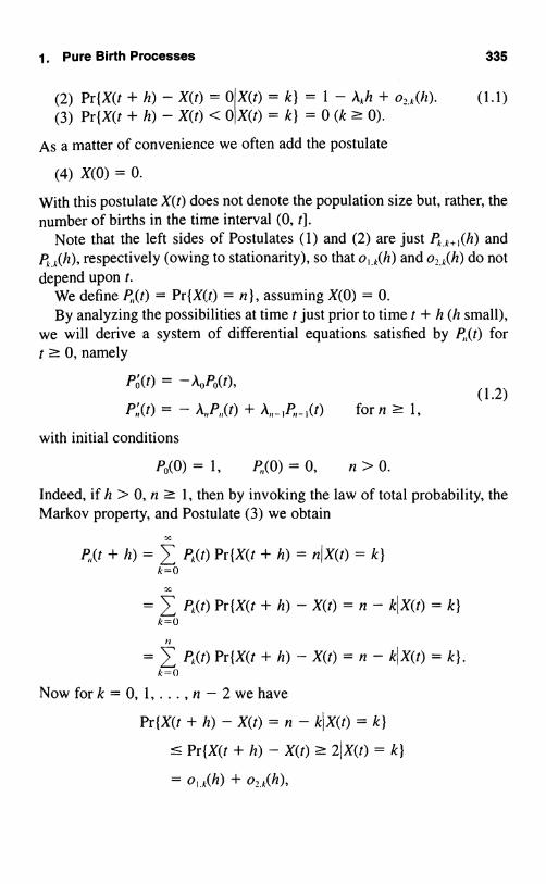
1. Pure Birth Processes 335
(2) Pr{X(t + h) - X(t) = 0(3) Pr{X(t + h) - X(t) < 0
X(t) = k) = 1 - 1tkh + o,.,(h). (1.1)X(t) = k} = 0 (k >_ 0).
As a matter of convenience we often add the postulate
(4) X(0) = 0.
With this postulate X(t) does not denote the population size but, rather, thenumber of births in the time interval (0, t}.
Note that the left sides of Postulates (1) and (2) are just P.k+,(h) andPA,x(h), respectively (owing to stationarity), so that o,,k(h) and o,.,(h) do notdepend upon t.
We define P(t) = Pr{X(t) = n}, assuming X(0) = 0.By analyzing the possibilities at time t just prior to time t + h (h small),
we will derive a system of differential equations satisfied by P(t) fort ? 0, namely
Pa(t) = -A0P0(t),(1.2)
P111(t) = - forn ? 1,
with initial conditions
PO(0) = 1, 0, n > 0.
Indeed, if h > 0, n ? 1, then by invoking the law of total probability, theMarkov property, and Postulate (3) we obtain
xh) = PR.(t) Pr(X(t + h) = nI X(t) = k}
k=0
PA.(t) Pr{X(t + h) - X(t) = n - kJX(t) = k}k=0
PA(t) Pr{X(t + h) - X(t) = n - k X(t) = k}.k=0
Now for k = 0, 1,...,n-2wehave
Pr{X(t + h) - X(t) = n - klX(t) = k}
Pr{X(t + h) - X(t) ? 21X(t) = k}
= o1.k(h) + o,.k(h),

336 VI Continuous Time Markov Chains
or
Pr(X(t + h) - X(t) = n - kjX(t) = k} = 03.,,,k(h), k= 0, ... , n - 2.Thus
h) = P(t)[1 - 02.,,(h)] + o,.,,_,(h)]
n-2
.or
h) -(1.3)
= o,,(h)] + oj.,,_1(h)l + o,,(h),
where, clearly, lim,,10 0 uniformly in t ? 0, since o,,(h) isbounded by the finite sum Jk=0 o3.n.k(h), which does not depend on t.
Dividing by h and passing to the limit h 10, we validate the relations(1.2), where on the left side we should, to be precise, write the derivativefrom the right. With a little more care, however, we can derive the samerelation involving the derivative from the left. In fact, from (1.3) we seeat once that the are continuous functions of t. Replacing t by t - h in(1.3), dividing by h, and passing to the limit h 10, we find that eachhas a left derivative that also satisfies equation (1.2).
The first equation of (1.2) can be solved immediately and yields
Define Sk as the time between the kth and the (k + 1)st birth, so that
n-1
S, :!s: t<S;
Po(t) = exp{-A0t} for t > 0. (1.4)
k=0
The random variables Sk are called the "sojourn times" between births,and
W=k-1
= the time at which the kth birth occurs.i=O
We have already seen that Po(t) = exp{-Aot}. Therefore,
Pr{S0 <- t} = 1 - Pr(X(t) = 0) = I - exp(-A0t);

1. Pure Birth Processes 337
i.e., So has an exponential distribution with parameter Ao. It may he deducedfrom Postulates (1) through (4) that Sk, k > 0, also has an exponential dis-tribution with parameter Ak and that the S;'s are mutually independent.
This description characterizes the pure birth process in terms of its so-journ times, in contrast to the infinitesimal description corresponding to
(1.1).To solve the differential equations of (1.2) recursively, introduce Q,,(t)
= for n = 0, 1, .... Then
Q;,(t) = A,,eA,1F,(t) +
P'(t)]
= [using (1.2)].
Integrating both sides of these equations and using the boundary condition0 for n ? 1 gives
r
f en°AA .P,-.(x) dx,0
or
1
P,(t) JeI-1(x) dx, n = 1, 2 , .... (1.5)0
It is now clear that all Pk(t) ? 0, but there is still a possibility that
7, 1.=0
To secure the validity of the process, i.e., to assure that 1 forall t, we must restrict the Ak according to the following:
xP(t) = 1 if and only if
=01
(1.6)
The intuitive argument for this result is as follows: The time Sk betweenconsecutive births is exponentially distributed with a corresponding para-meter Ak. Therefore, the quantity I 1/A,, equals the expected time beforethe population becomes infinite. By comparison, 1 - Y.;,=o is theprobability that X(t) = oo.

338 VI Continuous Time Markov Chains
If I A < oc, then the expected time for the population to become in-finite is finite. It is then plausible that for all t > 0 the probability thatX(t) = 00 is positive.
When no two of the birth parameters A,,, A,.... are equal, the integralequation (1.5) may be solved to give the explicit formula
PO(t) =
e - A"' + e- Ai',I AO
A,
1
Ao AO
1
- A, /
and
Pr{X(t) = nI X(0) = 0)
= AO ... A,,_I[Bo.,,e-A,,' + ... + B,,.,,e-A''] for n > 1,
where
1
Bo.,, = (AI _ AO) ... (All - AX
Bk',, (Ao AA.) ... (IA._ AA.)(AA.+I AA.) - - - l(A,, - A.A)
for 0 < k < n,
and
B =
(1.8)
1 (1.9)
1
,i.,, (Ao - (A,,-I -
Because A; Ak when j 0 k by assumption, the denominator in (1.9) doesnot vanish, and Bk.,, is well-defined.
We will verify that P,(t), as given by (1.7), satisfies (1.5). Equation(1.4) gives Po(t) = e-'°'. We next substitute this in (1.5) when n = 1,thereby obtaining
P, (t) =Aoe-A
, J eA,` e-A°.e a
0
= AI)I[1 _ e I,
= A 1 e All, + 1 e-O
A, - A. A - AI
in agreement with (1.7).

1. Pure Birth Processes 339
The induction proof for general n involves tedious and difficult algebra.The case n = 2 is suggested as a problem.
1.3. The Yule Process
The Yule process arises in physics and biology and describes the growthof a population in which each member has a probability f3h + o(h) of giv-ing birth to a new member during an interval of time of length h (/3 > 0).Assuming independence and no interaction among members of the popu-lation, the binomial theorem gives
Pr(X(t + h) - X(t) = 1I X(t) = n} = (n)[/3h + o(h)][l - f3h + o(h)]"-'
= n f3h +
i.e., for the Yule process the infinitesimal parameters are A,, = no. Inwords, the total population birth rate is directly proportional to the popu-lation size, the proportionality constant being the individual birth rate /3.As such, the Yule process forms a stochastic analogue of the determinis-tic population growth model represented by the differential equationdy/dt = ay. In the deterministic model, the rate dy/dt of population growthis directly proportional to population size y. In the stochastic model, theinfinitesimal deterministic increase dy is replaced by the probability of aunit increase during the infinitesimal time interval dt. Similar connectionsbetween deterministic rates and birth (and death) parameters arise fre-quently in stochastic modeling. Examples abound in this chapter.
The system of equations (1.2) in the case that X(0) = 1 becomes
P,',(t) _ - (n - n = 1, 2, ...
under the initial conditions
P,(0) = 1, 0, n = 2, 3. ... .
Its solution is
P(t) = e-1(1 - e-1)", n 1, (1.10)
as may be verified directly. We recognize (1.10) as the geometric distrib-ution 1, (3.5) with p = e-'*.

340 VI Continuous Time Markov Chains
The general solution analogous to (1.8) but for pure birth processesstarting from X(0) = 1 is
P,ft) = A, ... A,,-. [B1.,,e-A'' + ... n > 1. (1.11)
When A,, = /3n, we will show that (1.11) reduces to the solution given in(1.10) for a Yule process with parameter P. Then
1
Bl.u = (A,-AI)(A3-A1)...(A,, - AI)1
R I(1)(2) ... (n - 1)
P"-'(n - 1)!'
1
B,,,, = (A, - A,)(A3 - A) ... (A,, - A,)
I(-1)(1)(2) ... (n - 2)
-1
and
2)!'
(_ 1)k-I
P"-'(k - 1)!(n - k)!
Thus, according to (1.11),
P,(t) = P"-'(n - 1)!(B,.,,e-l1 + ... + B,,.,,e
11 (n - 1)!_ k - 1)!(n -
k)i(-1)k le k/tr
k=1
11-
(AI - Ak) ... (Ak-I - Ak)(Ak+l - Ak) ... (An - Ak)
(n - 1)! (-e-13r)
j=0 J!(n - 1 - J)!
1
= e -O(1 - e')" -I [see I, (6.17)],
which establishes (1.10).

Exercises 341
Exercises
1.1. A pure birth process starting from X(O) = 0 has birth parametersk = 1, A = 3, A, = 2, A, = 5. Determine for n = 0, 1, 2, 3.
1.2. A pure birth process starting from X(O) = 0 has birth parameters,, = 1, A, = 3, A, = 2, A, = 5. Let W, be the random time that it takes theprocess to reach state 3.
(a) Write W, as a sum of sojourn times and thereby deduce that themean time is E[W] = 6.
(b) Determine the mean of W, + W, + W.(c) What is the variance of W,?
1.3. A population of organisms evolves as follows. Each organism ex-ists, independent of the other organisms, for an exponentially distributedlength of time with parameter 0, and then splits into two new organisms,each of which exists, independent of the other organisms, for an expo-nentially distributed length of time with parameter 0, and then splits intotwo new organisms, and so on. Let X(t) denote the number of organismsexisting at time t. Show that X(t) is a Yule process.
1.4. Consider an experiment in which a certain event will occur withprobability ah and will not occur with probability 1 - ah, where a is afixed positive parameter and h is a small (h < 1/a) positive variable. Sup-pose that n independent trials of the experiment are carried out, and thetotal number of times that the event occurs is noted. Show that
(a) The probability that the event never occurs during the n trials is1 - nah + o(h);
(b) The probability that the event occurs exactly once is nah + o(h);(c) The probability that the event occurs twice or more is o(h).
Hint: Use the binomial expansion
(1 - ah)" = 1 - nah +n(n
2
- 1)(ah)2 -
1.5. Using equation (1.10), calculate the mean and variance for the Yuleprocess where X(0) = 1.

342 VI Continuous Time Markov Chains
1.6. Operations 1, 2, and 3 are to be performed in succession on a majorpiece of equipment. Operation k takes a random duration Sk that is expo-nentially distributed with parameter Ak for k = 1, 2, 3, and all operationtimes are independent. Let X(t) denote the operation being performed attime t, with time t = 0 marking the start of the first operation. Supposethat A, = 5, A, = 3, and A, = 13. Determine
(a) P,(t) = Pr{X(t) = 1).(b) P,(t) = Pr{X(t) = 2).(c) P,(t) = Pr{X(t) = 3}.
Problems
1.1. Let X(t) be a Yule process that is observed at a random time U,where U is uniformly distributed over [0, 1). Show that Pr{X(U) = k} _pk/(/3k) for k = 1, 2, . . . , with p = I - e-a.
Hint: Integrate (1.10) over t between 0 and 1.
1.2. A Yule process with immigration has birth parameters Ak = a + k/3for k = 0, 1, 2, .... Here a represents the rate of immigration into thepopulation, and 6 represents the individual birth rate. Supposing thatX(0) = 0, determine P(t) for n = 0, 1, 2, ... .
1.3. Consider a population comprising a fixed number N of individuals.Suppose that at time t = 0 there is exactly one infected individual andN - 1 susceptible individuals in the population. Once infected, an indi-vidual remains in that state forever. In any short time interval of length h,any given infected person will transmit the disease to any given suscepti-ble person with probability ah + o(h). (The parameter a is the individualinfection rate.) Let X(t) denote the number of infected individuals in thepopulation at time t ? 0. Then X(t) is a pure birth process on the states0, 1, . . . , N. Specify the birth parameters.
1.4. A new product (a "Home Helicopter" to solve the commuting prob-lem) is being introduced. The sales are expected to be determined by bothmedia (newspaper and television) advertising and word-of-mouth adver-tising, wherein satisfied customers tell others about the product. Assumethat media advertising creates new customers according to a Poissonprocess of rate a = 1 customer per month. For the word-of-mouth adver-

Problems 343
tising, assume that each purchaser of a Home Helicopter will generatesales to new customers at a rate of 0 = 2 customers per month. Let X(t)be the total number of Home Helicopter customers up to time t.
(a) Model X(t) as a pure birth process by specifying the birth parame-ters Ak, for k = 0, 1, ... .
(b) What is the probability that exactly two Home Helicopters are soldduring the first month?
1.5. Let W. be the time to the kth birth in a pure birth process startingfrom X(0) = 0. Establish the equivalence
Pr{W1 > t, W, > t.+ s} = P,(s)}.
From this relation together with equation (1.7), determine the joint den-sity for W, and W,, and then the joint density of S = W, and S, _W,-W,.
1.6. A fatigue model for the growth of a crack in a discrete latticeproposes that the size of the crack evolves as a pure birth process withparameters
Ak = (1 + k)'' for k = 1, 2. ... .The theory behind the model postulates that the growth rate of the crackis proportional to some power of the stress concentration at its ends, andthat this stress concentration is itself proportional to some power of1 + k, where k is the crack length. Use the sojourn time description to de-duce that the mean time for the crack to grow to infinite length is finitewhen p > 1, and that therefore the failure time of the system is a well-defined and finite-valued random variable.
1.7. Let A0, A, and A, be the parameters of the independent exponen-tially distributed random variables S,, S, and S,. Assume that no two ofthe parameters are equal.
(a) Verify that
Pr{So > t} = e-",,,
Pr{S + S, > t} _ ' e a',

344 VI Continuous Time Markov Chains
and evaluate in similar terms
Pr{Sa+S,+S2>t}.
(b) Verify equation (1.8) in the case that n = 2 by evaluating
P,(t)=Pr{X(t)=2}=Pr{So+S,+S,>t}-Pr{S0+S,>t}.
1.8. Let N(t) be a pure birth process for which
Pr{an event happens in (t, t + h)IN(t) is odd} = ah + o(h),
Pr{an event happens in (t, t + h)IN(t) is even} _ 6h + o(h),
where o(h)/h -* 0 as h 1 0. Take N(O) = 0. Find the followingprobabilities:
Po(t) = Pr{N(t) is even}; P,(t) = Pr(N(t) is odd}.
Hint: Derive the differential equations
Po(t) = aP,(t) - /3Po(t) and P,(t) = -aP,(t) + /3Po(t),
and solve them by using Po(t) + P,(t) = 1.
1.9. Under the conditions of Problem 1.8, determine E[N(t)].
1.10. Consider a pure birth process on the states 0, 1, . . . , N for whichA, = (N - k)A for k = 0, 1, . . . , N. Suppose that X(0) = 0. Determine
Pr{X(t) = n} for n = 0, 1, and 2.
1.11. Beginning with Pa(t) = e-a°' and using equation (1.5), calculateP,(t), P,(t), and P,(t) and verify that these probabilities conform with equa-tion (1.7), assuming distinct birth parameters.
1.12 Verify that P,(t), as given by (1.8), satisfies (1.5) by following thecalculations in the text that showed that P,(t) satisfies (1.5).
1.13. Using (1.5), derive when all birth parameters are the sameconstant A and show that
P (t) =(At)"e-a'
n=0,1, ...n!
Thus, the postulates of Section 1.1 serve to define the Poisson processes.

2. Pure Death Processes 345
2. Pure Death Processes
Complementing the increasing pure birth process is the decreasing puredeath process. It moves successively through states N, N - 1, . . . , 2, 1and ultimately is absorbed in state 0 (extinction). The process is specifiedby the death parameters µk > 0 for k = 1, 2, . . . , N, where the sojourntime in state k is exponentially distributed with parameter µk, all sojourntimes being independent. A typical sample path is depicted in Figure 2.1.
X(t)
NN-1N-2
2
1
SN
WI
SN- 1
W,
SI
t
Figure 2.1 A typical sample path of a pure death process, showing thesojourn times S , ,.. . , SI and the waiting times W, W2,. . . , WN.
Alternatively, we have the infinitesimal description of a pure deathprocess as a Markov process X(t) whose state space is 0, 1, ... , N and forwhich
(i) Pr(X(t + h) = k - 1I X(t) = k} = µkh + o(h), k = 1, ... , N;(ii) Pr{X(t + h) = kjX(t) = k} = 1 - µkh + o(h), k = 1, ... , N; (2.1)
(iii) Pr(X(t + h) > kjX(t) = k} = 0, k = 0, 1, . . . , N.
The parameter I-µ, is the "death rate" operating or in effect while theprocess sojourns in state k. It is a common and useful convention to assignAO=0.

346 VI Continuous Time Markov Chains
When the death parameters µ,, µ,, ... , µv are distinct, that is, p 0 g,if j k, then we have the explicit transition probabilities
P,,(t) = e-",';
and for n < N,
Pr{X(t) = nI X(0) = N)
where
1
µk) ... (AA +I - P-)(P- - I - Ak) ... (A - -k)
2.1. The Linear Death Process
(2.2)
As an example, consider a pure death process in which the death rates areproportional to population size. This process, which we will call the lin-ear death process, complements the Yule, or linear birth, process. The pa-rameters are µk = ka, where a is the individual death rate in the popula-tion. Then
1
(!L"' - A») ... (A", - A")
1
aN-"-'(N - n)(N - n - 1) ... (2)(1)'
1
(Av - (A,,12 - A,,+])
1
n - 1) ... (1)(-1),
1
(AN - Pk) ... (11k+1 - Pk)(P-k-I - N-k) ... (A - Pk)
1
= ai(N-k)...(1)(-1)(-2)...(n-k)1
k)!(k - n)!

2. Pure Death Processes 347
ThenN
µ4l
k=n
N! N e-ka1aA`-,1 I In! k=,,
aN-n )(-1)k -(N - k)!(k - n)!
N! -n 1ye-j°'= n! j=0 (N - n -,)!j!
N! e"'(1 - e-a1)N- n = 0, ... , N.n!(N - n)!
(2.3)
Let T be the time of population extinction. Formally, T = min{t ? 0;X(t) = 0). Then T:5 t if and only if X(t) = 0, which leads to the cumula-tive distribution function of T via
FT(t) = Pr{T < t} = Pr{X(t) = 0)
= P0(t) _ (1 - e-tt1)N, t ? 0.(2.4)
The linear death process can be viewed in yet another way, a way thatagain confirms the intimate connection between the exponential distribu-tion and a continuous time parameter Markov chain. Consider a popula-tion consisting of N individuals, each of whose lifetimes is an independentexponentially distributed random variable with parameter a. Let X(t) bethe number of survivors in this population at time t. Then X(t) is the lin-ear pure death process whose parameters are µk = ka for k = 0, 1, ... ,N. T o help understand this connection, let 6 6,, ... , ,,, denote the timesof death of the individuals labeled 1, 2, . . . , N, respectively. Figure 2.2,on the next page, shows the relation between the individual lifetimes
,, ... , 6N and the death process X(t).The sojourn time in state N, denoted by S, equals the time of the earli-
est death, or S, = min( 6,, . . . , 6A. } . Since the lifetimes are independentand have the same exponential distribution,
Pr{S,,,>t} N}>t}
=Pr{6,>t,...,6, >t}_ [Pr{6, > t}]'
e Na t

348 VI Continuous Time Markov Chains
N=65
4
3
2
I
{
I
EN
I
Time ofDeath
S
S4
S3
S2
W, W2 W3 W4 W5 WN t
Figure 2.2 The linear death process. As depicted here, the third individual isthe first to die, the first individual is the second to die, etc.
That is, SN has an exponential distribution with parameter Na. Similar rea-soning applies when there are k members alive in the population. Thememoryless property of the exponential distribution implies that the re-maining lifetime of each of these k individuals is exponentially distributedwith parameter a. Then the sojourn time Sk is the minimum of these k re-maining lifetimes and hence is exponentially distributed with parameterka. To give one more approach in terms of transition rates, each individ-ual in the population has a constant death rate of a in the sense that
Pr(t<6, <t+hit< ,} = <t+h)
ear - e-«(r+h)
e ar
=1-eah= ah + o(h) as h 1 0.
X 0)
N=65
4
3
2
1
S,

2. Pure Death Processes 349
If each of k individuals alive in the population at time t has a constantdeath rate of a, then the total population death rate should be ka, directlyproportional to the population size. This shortcut approach to specifyingappropriate death parameters is a powerful and often-used tool of sto-chastic modeling. The next example furnishes another illustration of itsuse.
2.2. Cable Failure Under Static Fatigue
A cable composed of parallel fibers under tension is being designed tosupport a high-altitude weather balloon. With a design load of 1000 kgand a design lifetime of 100 years, how many fibers should be used in thecable?
The low-weight, high-strength fibers to be used are subject to staticfatigue, or eventual failure when subjected to a constant load. The higherthe constant load, the shorter the life, and experiments have established alinear plot on log-log axes between average failure time and load that isshown in Figure 2.3.
The relation between mean life p, and load I that is illustrated in Fig-ure 2.3 takes the analytic form
log, A, = 2 - 40 log,ol.
log (time)
log (100 yrs)
-+--slope = -P= -40
log (1 kg) log (load)
Figure 2.3 A linear relation between log mean failure time and log load.

350 VI Continuous Time Markov Chains
Were the cable to be designed on the basis of average life, to achievethe 100 year design target each fiber should carry 1 kg. Since the total loadis 1000 kg, N = '-°,°-° = 1000 fibers should be used in the cable.
One might suppose that this large number (N = 1000) of fibers wouldjustify designing the cable based on average fiber properties. We shall seethat such reasoning is dangerously wrong.
Let us suppose, however, as is the case with many modern high-perfor-mance structural materials, that there is a large amount of random scatterof individual fiber lifetimes about the mean. How does this randomnessaffect the design problem?
Some assumption must be made concerning the probability distributiongoverning individual fiber lifetimes. In practice, it is extremely difficult togather sufficient data to determine this distribution with any degree of cer-tainty. Most data do show, however, a significant degree of skewness, orasymmetry. Because it qualitatively matches observed data and because itleads to a pure death process model that is accessible to exhaustive analy-sis, we will assume that the probability distribution for the failure time Tof a single fiber subjected to the time-varying tensile load l(t) is given by
t
Pr{T <_ t} = I - exp 1-f K[l(s)] ds , t ? 0.0
This distribution corresponds to a failure rate, or hazard rate, ofr(t) = K[l(t)] wherein a single fiber, having not failed prior to time t andcarrying the load 1(t), will fail during the interval (t, t + At] withprobability
Pr{t < T < t + WIT > t} = K[l(t)] At + o(At).
The function K[l], called the breakdown rule, expresses how changes inload affect the failure probability. We are concerned with the power lawbreakdown rule in which K[l] = 1'3/A for some positive constants A and /3.Assuming power law breakdown, under a constant load l(t) = 1, the singlefiber failure time is exponentially distributed with mean µ, = E[TJl] _1/K[l] = Al-1. A plot of mean failure time versus load is linear on log-logaxes, matching the observed properties of our fiber type. For the designproblem we have /3 = 40 and A = 100.

2. Pure Death Processes 351
Now place N of these fibers in parallel and subject the resulting bundleor cable to a total load, constant in time, of NL, where L is the nominalload per fiber. What is the probability distribution of the time at which thecable fails? Since the fibers are in parallel, this system failure time equalsthe failure time of the last fiber.
Under the stated assumptions governing single-fiber behavior, X(t), thenumber of unfailed fibers in the cable at time t, evolves as a pure deathprocess with parameters A, = kK[NLIk] for k = 1, 2, ... , N. GivenX(t) = k surviving fibers at time t and assuming that the total bundle loadNL is shared equally among them, then each carries load NL/k and has acorresponding failure rate of K[NL/k]. As there are k such survivors in thebundle, the bundle, or system, failure rate is µk = kK[NL/k] as claimed.
It was mentioned earlier that the system failure time was W,,,, the wait-ing time to the Nth fiber failure. Then Pr{W,,, S t} = Pr{X(t) = 0} = P,(t),where is given explicitly by (2.2) in terms of µ,, ... , µ,,,. Alterna-tively, we may bring to bear the sojourn time description of the pure deathprocess and, following Figure 2.1, write
+5,,
where SN, S, are independent exponentially distributed randomvariables and Sk has parameter µk = kK[NL/k] = k(NLIk)R/A. The meansystem failure time is readily computed to be
E[W,] = E[S,,,] + + E[S,]
x-, k
(k)"= AL-R N(2.5)
)R '( )
The sum in the expression for E[W,,] seems formidable at first glance, buta very close approximation is readily available when N is large. Figure 2.4compares the sum to an integral.
From Figure 2.4 on the next page we see that
(k)(i)N xR- 'dx=k_, N N

352 VI Continuous Time Markov Chains
llR - '(N/
0 1 2 3 H1H N-11 xN N N N N
Figure 2.4 The sum Yk , (kIN)a-'(1/N) is a Riemann approximationto f xs-' dx = 1//3.
Indeed, we readily obtain1 =f1 N (kl1 1+r1/N
/3 xa'dx I (-) :5 xR-'dx
()E(1 + N)R - (N)°I.
When N = 1000 and /3 = 40, the numerical bounds are
k N) (N) (40)(1.0408),
which shows that the integral determines the sum to within about 4percent.
Substituting 1/$ for the sum in (2.5) gives the average cable life
E[WN] A
to be compared with the average fiber life of
AµrLp.

Exercises 353
That is, a cable lasts only about 1//3 as long as an average fiber under anequivalent load. With A = 100, /3 = 40, and N = 1000, the designed cablewould last, on the average, 100/[40(1)40] = 2.5 years, far short of the de-sired life of 100 years. The cure is to increase the number of fibers in thecable, thereby decreasing the per fiber load. Increasing the numberof fibers from N to N' decreases the nominal load per fiber fromL to L' = NL/N'. To achieve parity in fiber-cable lifetimes we equate
A _ A
L[3 /3(NLIN' )s'
or
N' = N/3' .
For the given data, this calls for N' = 1000(40)" = 1097 fibers. That is,the design lifetime can be restored by increasing the number of fibers inthe cable by about 10 percent.
Exercises
2.1. A pure death process starting from X(0) = 3 has death parametersµ0 = 0, µ, = 3, p, = 2, µ, = 5. Determine for n = 0, 1, 2, 3.
2.2. A pure death process starting from X(0) = 3 has death parametersAo = 0, µ, = 3,A2= 2,A3 = 5. Let W, be the random time that it takesthe process to reach state 0.
(a) Write W, as a sum of sojourn times and thereby deduce that themean time is E[W,] = o.
(b) Determine the mean of W, + W, + W,.(c) What is the variance of W,?
2.3. Give the transition probabilities for the pure death process de-scribed by X(0) = 3, µ, = 1, p2 = 2, and µ, = 3.
2.4. Consider the linear death process (Section 2.1) in whichX(0) = N = 5 and a = 2. Determine Pr(X(t) = 2}.
Hint: Use equation (2.3).
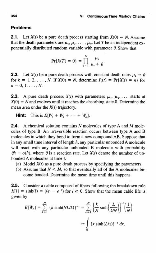
354 VI Continuous Time Markov Chains
Problems
2.1. Let X(t) be a pure death process starting from X(O) = N. Assumethat the death parameters are µ,, µ,, ... , µ,,,. Let T be an independent ex-ponentially distributed random variable with parameter 0. Show that
N
Pr{X(T) = 0}i=1 µ,+ 0
2.2. Let X(t) be a pure death process with constant death rates µ,. = 0for k = 1, 2, . . ., N. If X(O) = N, determine Pr(X(t) = n} forn=0,1,...,N.
2.3. A pure death process X(t) with parameters AI, p2, ... starts atX(O) = N and evolves until it reaches the absorbing state 0. Determine themean area under the X(t) trajectory.
Hint: This is E[W, + W + + WA,J.
2.4. A chemical solution contains N molecules of type A and M mole-cules of type B. An irreversible reaction occurs between type A and Bmolecules in which they bond to form a new compound AB. Suppose thatin any small time interval of length h, any particular unbonded A moleculewill react with any particular unbonded B molecule with probabilityOh + o(h), where 0 is a reaction rate. Let X(t) denote the number of un-bonded A molecules at time t.
(a) Model X(t) as a pure death process by specifying the parameters.(b) Assume that N < M, so that eventually all of the A molecules be-
come bonded. Determine the mean time until this happens.
2.5. Consider a cable composed of fibers following the breakdown ruleK[1] = sinh(l) = ;(e' - e-') for l L- 0. Show that the mean cable life isgiven by
E[W^,J = 7, {k sinh(NL/k)} ' = j N sinh(k/N)1 I Nk=I k=1 l `
- J {x sinh(L/x) } -' dx.0

3. Birth and Death Processes 355
2.6. Let T be the time to extinction in the linear death process with pa-rameters X(O) = N and a (see Section 2.1).
(a) Using the sojourn time viewpoint, show that
E[T]aLN+N1
1 +...+1J
(b) Verify the result of (a) by using equation (2.4) inx
E[T] = J Pr{T > t) dt = J [I - FT(t)] dt.0 0
Hint: Let y = 1 - e-°".
3. Birth and Death Processes
An obvious generalization of the pure birth and pure death processes dis-cussed in Sections 1 and 2 is to permit X(t) both to increase and to de-crease. Thus if at time t the process is in state n, it may, after a random so-journ time, move to either of the neighboring states n + 1 or n - 1. Theresulting birth and death process can then be regarded as the continuous-time analogue of a random walk (III, Section 5.3).
Birth and death processes form a powerful tool in the kit of the sto-chastic modeler. The richness of the birth and death parameters facilitatesmodeling a variety of phenomena. At the same time, standard methods ofanalysis are available for determining numerous important quantities suchas stationary distributions and mean first passage times. This section andlater sections contain several examples of birth and death processes andillustrate how they are used to draw conclusions about phenomena in a va-riety of disciplines.
3.1. Postulates
As in the case of the pure birth processes, we assume that X(t) is a Markovprocess on the states 0, 1, 2, ... and that its transition probabilities Pi(t)are stationary; i.e.,
P;(t) = Pr{X(t + s) = jjX(s) = i} for all s ? 0.

356 VI Continuous Time Markov Chains
In addition, we assume that the Pj(t) satisfy
(1) P,;,.,(h) = A;h + o(h) as h L 0, i ? 0;(2) P,;_,(h) = µ;h + o(h) as h .1 0, i ? 1;(3) P.;(h) = 1 - (A; + µ)h + o(h) as h 10, i ? 0;(4) Pj(O) = 5;;;(5) Ao=O,Ao>O,µ;,A;>O,i= 1,2,....
The o(h) in each case may depend on i. The matrix
_AO Ao 0 0 ...µ, -(A, + µ,) A, 0 ...
A= 0 µ,/
-(A,+µ,) A,, (3.1)
0
0
µ, -(A, + µ,) .. .
is called the infinitesimal generator of the process. The parameters A; andµ; are called, respectively, the infinitesimal birth and death rates. In Pos-tulates (1) and (2) we are assuming that if the process starts in state i, thenin a small interval of time the probabilities of the population increasing ordecreasing by 1 are essentially proportional to the length of the interval.
Since the Pj(t) are probabilities, we have Pj(t) ? 0 and
Pj(t) <- 1. (3.2)j=0
Using the Markov property of the process we may also derive the so-called Chapman-Kolmogorov equation
Pj(t + s) = Z, PR(t)PR;(s). (3.3)k=0
This equation states that in order to move from state i to state j in timet + s, X(t) moves to some state k in time t and then from k to j in theremaining time s. This is the continuous-time analogue of formula (2.2)in III.
So far we have mentioned only the transition probabilities Pj(t). Inorder to obtain the probability that X(t) = n, we must specify where theprocess starts or more generally the probability distribution for the initialstate. We then have

3. Birth and Death Processes 357
Pr{X(t) = n} _
q; = Pr{X(0) = i}.
3.2. Sojourn Times
With the aid of the preceding assumptions we may calculate the distribu-tion of the random variable Si, which is the sojourn time of X(t) in state i;that is, given that the process is in state i, what is the distribution of thetime Si until it first leaves state i? If we let
Pr{S, ? t} = G;(t),
it follows easily by the Markov property that as h 10,
Gi(t + h) = G;(t)G,(h) = G;(t)[R,;(h) + o(h)]
= G,(t)[1 - (A, + µ;)h] + o(h),
or
Gi(t + h) - G,(t)h
_ -(A, + µ)G;(t) + o(1),
so that
G(t) _ -(A1 + µ,)G,(t). (3.4)
If we use the conditions G;(0) = 1, the solution of this equation is
G;(t) = exp[-(A, + µ)t];
i.e., Si follows an exponential distribution with mean (A1 + µ;)-'. Theproof presented here is not quite complete, since we have used the intu-itive relationship
G,(h) = Pi(h) + o(h)
without a formal proof.According to Postulates (1) and (2), during a time duration of length h
a transition occurs from state i to i + 1 with probability A,h + o(h) andfrom state i to i - 1 with probability µ;h + o(h). It follows intuitively that,given that a transition occurs at time t, the probability that this transition

358 VI Continuous Time Markov Chains
is to state i + I is A;/(A; + µ;) and to state i - 1 is µ;l(A; + A j). The rig-orous demonstration of this result is beyond the scope of this book.
It leads to an important characterization of a birth and death process,however, wherein the description of the motion of X(t) is as follows: Theprocess sojourns in a given state i for a random length of time whose dis-tribution function is an exponential distribution with parameter (A; + µ;).When leaving state i the process enters either state i + I or state i - 1 withprobabilities A;/(A; + µ;) and µ;/(A; + µ;), respectively. The motion isanalogous to that of a random walk except that transitions occur at ran-dom times rather than at fixed time periods.
The traditional procedure for constructing birth and death processes isto prescribe the birth and death parameters { A;, µ;) =o and build the pathstructure by utilizing the preceding description concerning the waitingtimes and the conditional transition probabilities of the various states. Wedetermine realizations of the process as follows. Suppose X(O) = i; theparticle spends a random length of time, exponentially distributed withparameter (A; + A,), in state i and subsequently moves with probabilityA;/(A; + p,) to state i + 1 and with probability p,/(A; + µ;) to state i - 1.Next the particle sojourns a random length of time in the new state andthen moves to one of its neighboring states, and so on. More specifically,we observe a value t, from the exponential distribution with parameter(A; + p) that fixes the initial sojourn time in state i. Then we toss a coinwith probability of heads p; = A;/(A; + µ;). If heads (tails) appears wemove the particle to state i + 1 (i - 1). In state i + 1 we observe a valuet, from the exponential distribution with parameter (A;+, + µ;+,) that fixesthe sojourn time in the second state visited. If the particle at the first tran-sition enters state i - 1, the subsequent sojourn time t; is an observationfrom the exponential distribution with parameter (A;_, + µ;_,). After thesecond wait is completed, a Bernoulli trial is performed that chooses thenext state to be visited, and the process continues in the same way.
A typical outcome of these sampling procedures determines a realiza-tion of the process. Its form might be, for example,
i, for 0<t<ti + 1, fort, <t<t,+t,,
X(t)i, fort, +t,<t<t,+t,+t,,

3. Birth and Death Processes 359
Thus by sampling from exponential and Bernoulli distributions appropri-ately, we construct typical sample paths of the process. Now it is possibleto assign to this set of paths (realizations of the process) a probabilitymeasure in a consistent way so that P;(t) is determined satisfying (3.2) and(3.3). This result is rather deep, and its rigorous discussion is beyond thelevel of this book. The process obtained in this manner is called the min-imal process associated with the infinitesimal matrix A defined in (3.1).
The preceding construction of the minimal process is fundamental,since the infinitesimal parameters need not determine a unique stochasticprocess obeying (3.2), (3.3), and Postulates 1 through 5 of Section 3.1. Infact, there could be several Markov processes that possess the same infin-itesimal generator. Fortunately, such complications do not arise in themodeling of common phenomena. In the special case of birth and deathprocesses for which A0 > 0, a sufficient condition that there exists aunique Markov process with transition probability function P;(t) forwhich the infinitesimal relations (3.2) and (3.3) hold is that
where
0,,
00= 1, n= 1,2,....µiµ2 ... An
(3.5)
In most practical examples of birth and death processes the condition(3.5) is met, and the birth and death process associated with the prescribedparameters is uniquely determined.
3.3. Differential Equations of Birth and Death Processes
As in the case of the pure birth and pure death processes, the transitionprobabilities P;(t) satisfy a system of differential equations known as thebackward Kolmogorov differential equations. These are given by
Poi(t) _ AoP,,j(t) + k P,j(t), (3.6)
P;;(t) = I-p,P-'.;(t) - R + WPM) + A,P+1.;(t), i ? 1,
and the boundary condition P;(0) = 5;;.

360 VI Continuous Time Markov Chains
To derive these we have, from equation (3.3),x
Pj(t + h) = 7, Pk(h)Pj(t)k=0
= P.i-.(h)P-..j(t) + P.i(h)Pj(t) +.P.i+.(h)P+..j(t)(3.7)
+ Y-kPik(h)Pkj(t),
where the last summation is over all k 0 i - 1, i, i + 1. Using Postulates1, 2, and 3 of Section 3.1, we obtain
II F (h)Pj(t) C 4k Pk(h)
= 1 - [P,.i(h) + P.i-.(h) + P.i+.(h)]
= I - [1 - (Ai + µi)h + o(h) + µih + o(h) + Aih + o(h)]
= o(h),
so that
Pj(t + h) = µihP_,,j(t) + [1 - (A, + p.)h]Pj(t) + AihPi+,.j(t) + o(h).
Transposing the term P1 (t) to the left-hand side and dividing the equationby h, we obtain, after
lettingh 10(,
ppP;;(t) = /L.F-..j(t) - (Ai + p..)rij(t) + AiP+1.j(t)
The backward equations are deduced by decomposing the time interval(0, t + h), where h is positive and small, into the two periods
(0, h), (h, t + h)
and examining the transition in each period separately. In this sense thebackward equations result from a "first step analysis," the first step beingover the short time interval of duration h.
A different result arises from a "last step analysis," which proceeds bysplitting the time interval (0, t + h) into the two periods
(0, t), (t, t + h)
and adapting the preceding reasoning. From this viewpoint, under morestringent conditions we can derive a further system of differentialequations

3. Birth and Death Processes 361
Pio(t) = -AoI.o(t) + p.1Pj.1(t),
P,j(t) = (Aj + µj)Pj(t) + Aj+IP.j+1(t),(3.8)
with the same initial condition Pj(0) = S;j. These are known as the forwardKolmogorov differential equations. To derive these equations we inter-change t and h in equation (3.7), and under stronger assumptions in addi-tion to Postulates (1), (2), and (3) it can be shown that the last term isagain o(h). The remainder of the argument is the same as before. The use-fulness of the differential equations will become apparent in the examplesthat we study in this and the next section.
A sufficient condition that (3.8) hold is that [Pkj(h)]/h = o(l) for k = j,j - 1, j + 1, where the o(l) term apart from tending to zero is uniformlybounded with respect to k for fixed j as h - 0. In this case it can be provedthat 14. Pk(t)Pkj(h) = o(h).
Example Linear Growth with Immigration A birth and death processis called a linear growth process if A,, = An + a and µ = An with A > 0,µ > 0, and a > 0. Such processes occur naturally in the study of biolog-ical reproduction and population growth. If the state n describes the cur-rent population size, then the average instantaneous rate of growth isAn + a. Similarly, the probability of the state of the process decreasing byone after the elapse of a small duration of time h is pnh + o(h). The fac-tor An represents the natural growth of the population owing to its currentsize, while the second factor a may be interpreted as the infinitesimal rateof increase of the population due to an external source such as immigra-tion. The component µn, which gives the mean infinitesimal death rate ofthe present population, possesses the obvious interpretation.
If we substitute the above values of A,, and µ in (3.8), we obtain
Pia(t) = -aJo(t) + µl'1(t),
P',.j(t) = [A(j - 1) + a]P.j-1(t) - [(A + p)j + a]Pj(t)
+ pA + 1)I'.j+1(t), j ? 1.Now, if we multiply the jth equation by j and sum, it follows that the ex-pected value
E[X(t)] = M(t) = L jPj(t)j=1
satisfies the differential equation

362 VI Continuous Time Markov Chains
M'(t) = a + (A - µ)M(t),
with initial condition M(0) = i, if X(O) = i. The solution of this equationis
M(t)=at+i ifA=µ,and
M(t) = a {e'a-"" - 1} + ie`A-'A)t if A 0 µ. (3.9)A - µ
The second moment, or variance, may be calculated in a similar way. It isinteresting to note that M(t) - oo as t - x if A ? µ, while if A < µ, themean population size for large t is approximately
aµ-11
These results suggest that in the second case, wherein A < µ, the pop-ulation stabilizes in the long run in some form of statistical equilibrium.Indeed, it can be shown that a limiting probability distribution {7r;} existsfor which lim, P, (t) _ i7 , j = 0, 1, .... Such limiting distributions forgeneral birth and death processes are the subject of Section 4.
Example The Two State Markov Chain Consider a Markov chain{X(t)} with state 10, 1) whose infinitesimal matrix is
0 1ARR
(3.10)
The process alternates between states 0 and 1. The sojourn times in state0 are independent and exponentially distributed with parameter a. Thosein state 1 are independent and exponentially distributed with parameter P.This is a finite state birth and death process for which A, = a, A, = 0,µo = 0 and µ, _ /3. The first Kolmogorov forward equation in (3.8)becomes
P ,(t) = -aP.(t) + $P0,(t). (3.11)
Now, PP,(t) = 1 - P,(t), which placed in (3.11) gives
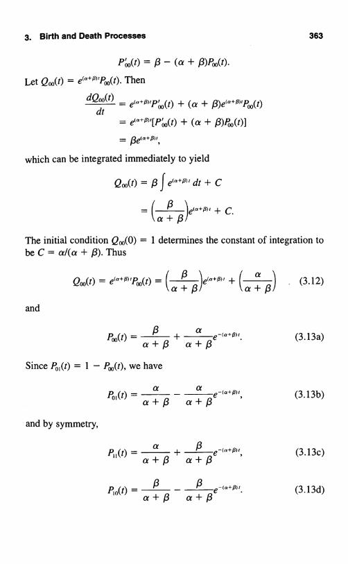
3. Birth and Death Processes 363
Pm(t) = /3 - (a + /3)A(t).
Let Q00(t) = e(a+p)'POO(t). Then
dQ.O(t)
dt= (a + R)e(a+R),POO(t)
= e(a+R),[Pa)(t) + (a + l3)Poo(t)]
= ae(a+p),N ,
which can be integrated immediately to yield
QO,(t) = 0 J e(`9)` dt + C
The initial condition Q,(0) = 1 determines the constant of integration tobe C = a/(a + /3). Thus
and
Pm(t)a f3
+a
+Re-c«+p, (3.13a)
( / e(a+p), + C.\a+/3)
Since P0#) = 1 - Pm(t), we have
PA)(t) =a a
(3.13b)
and by symmetry,
a+/3 a+/3 '
p)(t) = a + R e (a+p),
a+(3 a+ (3.13c)
pi(t) = a 0 R- a 0 Re-(a+p),. (3.13d)

364 Vf Continuous Time Markov Chains
These transition probabilities assume a more succinct form if we repa-rametrize according to 7r = a/(a + /3) and r = a + P. Then
Pm(t) _ (1 - IT) + 7re-7', (3.14a)
Pa, (t) = Ir - ITe-71, (3.14b)
P10(t) _ (1 - Ir) - (1 - ir)e-T', (3.14c)
and
IT + (1 - 7r)e-r'. (3.14d)
Observe that
lim P01(t) = lim Ir,
so that ir is the long run probability of finding the process in state 1 inde-pendently of where the process began. The long run behavior of generalbirth and death processes is the subject of the next section.
Exercises
3.1. Particles are emitted by a radioactive substance according to a Pois-son process of rate A. Each particle exists for an exponentially distributedlength of time, independent of the other particles, before disappearing. LetX(t) denote the number of particles alive at time t. Argue that X(t) is a birthand death process, and determine the parameters.
3.2. Patients arrive at a hospital emergency room according to° a Pois-son process of rate A. The patients are treated by a single doctor on a firstcome, first served basis. The doctor treats patients more quickly when thenumber of patients waiting is higher. An industrial engineering time studysuggests that the mean patient treatment time when there are k patients inthe system is of the form mk =a - /3k/(k + 1), where a and /3 are con-stants with a > /3 > 0. Let N(t) be the number of patients in the systemat time t (waiting and being treated). Argue that N(t) might be modeled asa birth and death process with parameters A,, = A for k = 0, 1, . . . andµ,. = k/m, for k = 0, 1..... State explicitly any necessary assumptions.

Problems 365
3.3. Let {V(t) } be the two state Markov chain whose transitionprobabilities are given by (3.14a-d). Suppose that the initial distributionis (1 - ir, 7r). That is, assume that Pr{ V(0) = 01 = 1 - 7r andPr{V(0) = 11 = 7r. In this case, show that Pr{V(t) = 1 } = 7r for all timest > 0.
Problems
3.1. Let 6,,, n = 0, 1, ... , be a two state Markov chain with transitionprobability matrix
F=0
Let {N(t); t ? 0) be a Poisson process with parameter A. Show that
X(t) = Sev(r), t j 0,is a two state birth and death process and determine the parameters Ao andµ, in terms of a and A.
3.2. Collards were planted equally spaced in a single row in order toprovide an experimental setup for observing the chaotic movements of theflea beetle (P. cruciferae). A beetle at position k in the row remains on thatplant for a random length of time having mean mk (which varies with the"quality" of the plant) and then is equally likely to move right (k + 1) orleft (k - 1). Model the position of the beetle at time t as a birth and deathprocess having parameters Ak = µk = 1/(2mk) for k = 1, 2, ... , N - 1,where the plants are numbered 0, 1, . . . , N. What assumptions might beplausible at the ends 0 and N?
3.3. Let {V(t) } be the two state Markov chain whose transition proba-bilities are given by (3.14a-d). Suppose that the initial distribution is(1 - ir, 7r). That is, assume that Pr { V(0) = 0) = 1 - rr andPr(V(0) = I) = nr. For 0 < s < t, show that
E[V(s)V(t)] = 1r - arPa(t - s),
whence
Cov[V(s), V(t)] = 1r(1 - 7r)e-(°+'3' ` '

366 VI Continuous Time Markov Chains
3.4. A Stop-and-Go Traveler The velocity V(t) of a stop-and-go trav-eler is described by the two state Markov chain whose transition proba-bilities are given by (3.14a-d). The distance traveled in time t is the inte-gral of the velocity:
S(t) = f V(u) du.0
Assuming that the velocity at time t = 0 is V(0) = 0, determine the meanof S(t). Take for granted the interchange of integral and expectation in
t
E[S(t)] = f E[V(u)] du.0
4. The Limiting Behavior of Birth andDeath Processes
For a general birth and death process that has no absorbing states, it canbe proved that the limits
lim P,.;(t) = ?r; ? 0 (4.1)!fix
exist and are independent of the initial state i. It may happen that 1r; = 0for all states j. When the limits 17) are strictly positive, however, and satisfy
= 1, (4.2)
I=0
they form a probability distribution that is called, naturally enough, thelimiting distribution of the process. The limiting distribution is also a sta-tionary distribution in that
x
1; = X. ir,P,(t),i=0
(4.3)
which tells us that if the process starts in state i with probability ir;, thenat any time t it will be in state i with the same probability ir;. The proof of(4.3) follows from (3.3) and (4.1) if we let t x and use the fact that
x

4. The Limiting Behavior of Birth and Death Processes 367
The general importance of birth and death processes as models derivesin large part from the availability of standard formulas for determining ifa limiting distribution exists and what its values are when it does. Theseformulas follow from the Kolmogorov forward equations (3.8) that werederived in Section 3.3:
Pi.o(t) _ -A0P.o(t) + Ail'.i(t), (4.4)
P/i.j(t) = Aj-IPj.j-I(t) - (Aj + Aj)Pij(t) + 1jj+Irr.j+I(t), 1,
with the initial condition i,(0) = Sij. Now pass to the limit as t oo in
(4.4) and observe first that'\the limit of the right side of (4.4) exists ac-cording to (4.1). Therefore, the limit of the left side, the derivatives P;j(t),exists as well. Since the probabilities are converging to a constant, thelimit of these derivatives must be zero. In summary, passing to the limit in(4.4) produces
0 = -AoiTo + µ11T1,
0 = Aj-i'7Tj-i - (Aj + /j'j).7Tj + !-_j+i1Tj+i, j 1.
The solution to (4.5) is obtained by induction. Letting
00 = 1 and/LI IJ.2 ... µj
- AoA,... A3_,
(4.5)
for j ? 1, (4.6)
we have ir, = Aoirolµ, = O,,7ro. Then, assuming that l'k = 6k7ro fork = 1,...,j,weobtain
µj+iij+i = (Aj + N-j)Ojir0 - A1_101 ,Tro
= A03ir() + (µ3e3 - AA_,O,_,)iro
= A303iro,
and finally
1Tj+1 = Oj+i7To
In order that the sequence { 7rj } define a distribution, we must haveI.3 7r3 = 1. If 1 03 < x, then we may sum the following,

368 V1 Continuous Time Markov Chains
Ira = 007TO
IT, = 0,1xO
?T2 = 029r0
1 = (I 0k) IT0
to see that IT0 = 0k, and then
7r; = 0;7r0 =e;
x for j = 0, 1, .... (4.7)Ik=0 dk
If E dk = oo, then necessarily vr0 = 0, and then Tr; = 0;ir0 = 0 for all j, andthere is no limiting distribution (lim,,, P,.;(t) = 0 for all j).
Example Linear Growth with Immigration As described in theexample at the end of Section 3.3, this process has birth parametersA,, = a + An and death parameters µ = µn for n = 0, 1, . . . , whereA > 0 is the individual birth rate, a > 0 is the rate of immigration into thepopulation, and µ > 0 is the individual death rate.
Suppose A < µ. It was shown in Section 3.3 that the population meanM(t) converges to a/(µ - A) as t - oo. Here we will determine the limit-ing distribution of the process under the same condition A < µ.
Then 00 = 1, 0, = altk, 0, = a(a + A)l[A(21k)], 03 = a(a + A)(a + 2A)/[µ(2µ)(31x)], and, in general,
a(a + A) . . . [a + (k - 1)A]Bk
µk(k)!
- (alA)[(alA) + 1] ... [(alA) + k - 1] / A\kk! µ
((a/A)
kk
- l1(µlk
Now use the infinite binomial formula (I, equation (1.71)),
IN+k- 1\(1 - x)-" _ k Ixk for Ixl < 1,
k=0

4. The Limiting Behavior of Birth and Death Processes 369
to determine that
x
k= 0
k- 1/\µ) - (1 - Y
",A)
when A < A. Thus iro = (1 - .Vµ)"', and
,A R (a/A)[(a/A) + 1 ] ... [(alA) + k - 1 ]
fork > 1.
Example Repairman Models A system is composed of N machines,of which at most M <_ N can be operating at any one time. The rest are"spares." When a machine is operating, it operates a random length oftime until failure. Suppose this failure time is exponentially distributedwith parameter A.
When a machine fails, it undergoes repair. At most R machines can be"in repair" at any one time. The repair time is exponentially distributedwith parameter A. Thus a machine can be in any of four states: (i) operat-ing; (ii) "up," but not operating, i.e., a spare; (iii) in repair; (iv) waiting forrepair. There is a total of N machines in the system. At most M can be op-erating. At most R can be in repair.
The action is diagrammed in Figure 4.1 on the next page.Let X(t) be the number of machines "up" at time t, either operating orspare. Then (we assume) the number operating is min{X(t), M}, and thenumber of spares is max{0, X(t) - M}. Let Y(t) = N - X(t) be the num-ber of machines "down." Then the number in repair is min{Y(t), R}, andthe number waiting for repair is max{0, Y(t) - R). The foregoing formu-las permit us to determine the number of machines in any category, onceX(t) is known.
Then X(t) is a finite state birth and death process' with parameters
A,,=AXmin{N-n,R}AR for n = 0, 1, . . . , N - R,
{A(N-n) forn =N - R+ 1,...,N,
' The definition of birth and death processes was given for an infinite number of states.The adjustments in the definitions and analyses for the case of a finite number of states arestraightforward and even simpler than the original definitions, and are left to the reader.

370 VI Continuous Time Markov Chains
000000
FACTORY
Capacity = MFailure Rate = p.
"Spares"000
k
X(t) = Number of machines "up"
Waitingfor
repair000
REPAIR SHOP
Capacity = RRepair Rate = K
0000
Y (t) = Number of machines "down"
and
Figure 4.1 Repairman model.
µn forn=0,1,... ,M,min{n, M} ={µM forn=M+ 1,...,N.
It is now a routine task to determine the limiting probability distribu-tion for any values of A, µ, N, M, and R. (See Problems 4.1 and 4.7.) Interms of the limiting probabilities iro, 7r ... , arv, some quantities of in-terest are the following:
Average Machines Operating = 7r, + 21r, + + Mir
+ M(lrM+I
+ ... + 'TV);
Long Run Utilization =Average Machines Operating
Capacity
Tr, + 27r, + + MaM
+ (IT,r+, + ... + Irv);

4. The Limiting Behavior of Birth and Death Processes 371
Average Idle Repair Capacity = 1,7r,-,,, + 21rN-R+2 + + R7rN.
These and other similar quantities can be used to evaluate the desir-ability of adding additional repair capability, additional spare machines,and other possible improvements.
The stationary distribution assumes quite simple forms in certain spe-cial cases. For example, consider the special case in which M = N = R.The situation arises, for instance, when each machine's operator becomesits repairman upon its failure. Then A,, = A(N - n) and µ = µn forn = 0, 1, ... , N, and following (4.6), we determine 00 = 1, 0, = AN/µ,02 _ (AN)A(N - 1)/µ(2µ), and, in general,
N(N-1) (N k+1) A" A `
(1)(2 ... (k) -) - \ k 1\-)The binomial formula (1 + x)" _ Ik=o (k)x' applies to yield
N N 'k )N.
k=O =O M%)'Thus ir0 = [I + (A/µ)] ' _ [µl(A + µ)]N, and
'77i
-(k
)( l.t)]N
(k)\A+µ)k(A+µ)vk
We recognize (4.8) as the familiar binomial distribution.
(4.8)
Example Logistic Process Suppose we consider a population whosesize X(t) ranges between two fixed integers N and M (N < Al) for allt 0. We assume that the birth and death rates per individual at time t aregiven by
A = a(M - X(t)) and µ = f3(X(t) - N),
and that the individual members of the population act independently ofeach other. The resulting birth and death rates for the population then be-come
A,, = an(M - n) and µ = f3n(n - N).

372 VI Continuous Time Markov Chains
To see this we observe that if the population size X(t) is n, then each of then individuals has an infinitesimal birth rate A, so that A = an(M - n). Thesame rationale applies in the interpretation of the µ,,.
Under such conditions one would expect the process to fluctuate be-tween the two constants N and M, since, for example, if X(t) is near M, thedeath rate is high and the birth rate low, and then X(t) will tend toward N.Ultimately the process should display stationary fluctuations between thetwo limits N and M.
The stationary distribution in this case is
c Mm lN+,» - N + m ( /n
)(a
where c is an appropriate constant determined so that ITN+,,, = 1. To see
this, we observe that
ANA,N+, . AN+m-ION+m =
AN+il.LN+2 AN +m
of"N(N+ 1)
1) ... (N + m)m!
N+Jm\MmNI(R)m
Example Some Genetic Models Consider a population consisting ofN individuals that are either of gene type a or gene type A. The state ofthe process X(t) represents the number of a-individuals at time t. We as-sume that the probability that any individual dies and is replaced by an-other during the time interval (t, t + h) is Ah + o(h) independent of thevalues of X(t) and that the probability of two or more changes occurringin a time interval h is o(h).
The changes in the population structure are effected as follows. Anindividual is to be replaced by another chosen randomly from the popula-tion; i.e., if X(t) = j, then an a-type is selected to be replaced with proba-bility j/N and an A-type with probability 1 - j/N. We refer to this stage asdeath. Next, birth takes place by the following rule. Another selection ismade randomly from the population to determine the type of the new in-

4. The Limiting Behavior of Birth and Death Processes 373
dividual replacing the one that died. The model introduces mutation pres-sures that admit the possibility that the type of the new individual may bealtered upon birth. Specifically, let y, denote the probability that an a-typemutates to an A-type, and let y, denote the probability of an A-type mu-tating to an a-type.
The probability that the new individual added to the population is oftype a is
-yO+(1-N)y,. (4.9)
We deduce this formula as\follows: The probability that we select an a-type and that no mutation occurs is (j/N)(1 - y,). Moreover, the final typemay be an a-type if we select an A-type that subsequently mutates into ana-type. The probability of this contingency is (1 - j/N)y2. The combina-tion of these two possibilities gives (4.9).
We assert that the conditional probability that X(t+) - X(t) = 1 whena change of state occurs is
(1 N)[N(l y,) + (1 - N)y,J, where X(t) = j. (4.10)
In fact, the a-type population size can increase only if an A-type dies (isreplaced). This probability is 1 - (j/N). The second factor is the proba-bility that the new individual is of type a as in (4.9).
In a similar way we find that the conditional probability thatX(t+) - X(t) = -1 when a change of state occurs is
NN)(1 - y2) + N y, where X(t) = j.
The number of type a individuals in the population is thus a birth anddeath process with a finite number of states and infinitesimal birth anddeath rates
1t; = A(I fl-.(l Y') + (1 - N)y,JN
and

374 VI Continuous Time Markov Chains
µ, = lNCNY, + (1 - N)(1 - Yz)]N, 0 j < N.
Although these parameters seem rather complicated, it is interesting tosee what happens to the stationary measure {lrk}k_o if we let the popula-tion size N --> oo and the probabilities of mutation per individual y, and y,tend to zero in such a way that y,N - K, and y,N -4 K,, where 0 < K,,K, < c. At the same time, we shall transform the state of the process tothe interval [0, 1] by defining new states j/N, i.e., the fraction of a-typesin the population. To examine the stationary density at a fixed fraction x,where 0 < x < 1, we shall evaluate ark as k -4 oo in such a way thatk = [xN], where [xN] is the greatest integer less than or equal to xN.
Keeping these relations in mind we write
A(N J) .( a) NA.=- -y,)J +, whereas Yz
N (1 YIJ YI-Yz
and
( b ) Nµj _ A(N
) 1 - ) ' 1 + where b = YN J ( YI - YzJ N_j 1_y - Y-2,
Thenk-1
log 0k = log A - log µjj=o j=1
k-1 a k-1 b
)+logNaj=1 J=1 N -J
- log(N - k)k(1 +N
bk
).
Now, using the expansion3
log(l + x) = x - 22
+ 3 - , IxI < 1,
it is possible to writek-1 ( a) k-I 1
log 1+- =a-+ck,j=1 J j=I J

4. The Limiting Behavior of Birth and Death Processes 375
where c, approaches a finite limit as k - x. Therefore, using the relationk-I 1
7',----log k askl=1
we havek-I
7, log (1 + log k"+c,. ask-4 oo.
In a similar way we obtain
k-Ilog(1 +
N
b) log
(N
N'k),, + d, ask - x,
j=1 jwhere d, approaches a finite limit as k - x. Using the above relations wehave
log 9, - log (C,k" (N - k)''Na l
as k x,I'(N - k)k) (4.11)
where log C, = c, + d which approaches a limit, say C, as k - x. Noticethat a - K, and b -3 K, as N -3 x. Since k = [Nx], we have, for N -+ x,
0, - CK,NK,-IxK,-1(1 - x)K,-'.
Now, from (4.11) we have)b- i
0, - aC,k '(Ik
N.
Therefore,
Since C, ---> C as k tends to x, we recognize the right side as a Riemannsum approximation of
K,C f x"2-'(1 - x)KH-' dx.n
Thus
N 1
9; N"2K,C f x"2-1(1 - x)"'-' dx,r=o o
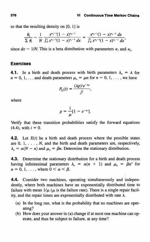
376 VI Continuous Time Markov Chains
so that the resulting density on [0, 11 is
Je4. 1
XKi-'(I - X)X'-1 XKi-I(1 - X)K,-I dX
10, N fo XK2-i(1 - X)K, dx fo XK,-i(1 - X)K,_, dx'
since dx 1/N. This is a beta distribution with parameters K, and K_
Exercises
4.1. In a birth and death process with birth parameters A,, = A forn = 0, 1, ... and death parameters µ = An for n = 0, 1, ... , we have
Po,(t)= (Ap);e-a"
J!
where
1
P = -[I - e-"1µ
Verify that these transition probabilities satisfy the forward equations(4.4), with i = 0.
4.2. Let X(t) be a birth and death process where the possible statesare 0, 1, . . . , N, and the birth and death parameters are, respectively,A,, = a(N - n) and µ = On. Determine the stationary distribution.
4.3. Determine the stationary distribution for a birth and death processhaving infinitesimal parameters A,, = a(n + 1) and µ = /3n2 forn = 0, 1, ...,where 0<a</i.
4.4. Consider two machines, operating simultaneously and indepen-dently, where both machines have an exponentially distributed time tofailure with mean 1/µ (p. is the failure rate). There is a single repair facil-ity, and the repair times are exponentially distributed with rate A.
(a) In the long run, what is the probability that no machines are oper-ating?
(b) How does your answer in (a) change if at most one machine can op-erate, and thus be subject to failure, at any time?

Problems 377
4.5. Consider the birth and death parameters A,, = 0 < 1, andnl(n + 1) for n = 0, 1. .... Determine the stationary distribution.
4.6. A birth and death process has parameters A,, = A and µ = nµ, forn = 0, 1. .... Determine the stationary distribution.
Problems
4.1. For the repairman model of the second example of this section,suppose that M = N = 5,R = 1, A = 2, and µ = 1. Using the limitingdistribution for the system, determine
(a) The average number of machines operating.(b) The equipment utilization.(c) The average idle repair capacity.
How do these system performance measures change if a second repairmanis added?
4.2. Determine the stationary distribution, when it exists, for a birth anddeath process having constant parameters A,, = A for n = 0, 1, ... and
n= 1,2.....
4.3. A factory has five machines and a single repairman. The operatingtime until failure of a machine is an exponentially distributed randomvariable with parameter (rate) 0.20 per hour. The repair time of a failedmachine is an exponentially distributed random variable with parameter(rate) 0.50 per hour. Up to five machines may be operating at any giventime, their failures being independent of one another, but at most one ma-chine may be in repair at any time. In the long run, what fraction of timeis the repairman idle?
4.4. This problem considers a continuous time Markov chain model forthe changing pattern of relationships among members in a group. Thegroup has four members: a, b, c, and d. Each pair of the group may or maynot have a certain relationship with each other. If they have the relation-ship, we say that they are linked. For example, being linked may mean thatthe two members are communicating with each other. The following

378 VI Continuous Time Markov Chains
graph illustrates links between a and b, between a and c, and betweenb and d:
Figure 4.2
Suppose that any pair of unlinked individuals will become linked in asmall time interval of length h with probability ah + o(h). Any pair oflinked individuals will lose their link in a small time interval of length hwith probability /3h + o(h). Let X(t) denote the number of linked pairs ofindividuals in the group at time t. Then X(t) is a birth and death process.
(a) Specify the birth and death parameters Ak and /j,, for k = 0, 1.... .(b) Determine the stationary distribution for the process.
4.5. A chemical solution contains N molecules of type A and an equalnumber of molecules of type B. A reversible reaction occurs between typeA and B molecules in which they bond to form a new compound AB. Sup-pose that in any small time interval of length h, any particular unbondedA molecule will react with any particular unbonded B molecule with prob-ability ah + o(h), where a is a reaction rate of formation. Suppose alsothat in any small time interval of length h, any particular AB molecule dis-associates into its A and B constituents with probability j3h + o(h), where,6 is a reaction rate of dissolution. Let X(t) denote the number of AB mol-ecules at time t. Model X(t) as a birth and death process by specifying theparameters.
4.6. A time-shared computer system has three terminals that are at-tached to a central processing unit (CPU) that can simultaneously handleat most two active users. If a person logs on and requests service whentwo other users are active, then the request is held in a buffer until it canreceive service. Let X(t) be the total number of requests that are either ac-tive or in the buffer at time t. Suppose that X(t) is a birth and death processwith parameters

5. Birth and Death Processes with Absorbing States 379
_ (A for k = 0, 1, 2,Ak
0 fork ? 3;
and
µk-Jkµ for k = 0, 1, 2,2µ fork=3.
Determine the long run probability that the computer is fully loaded.
4.7. A system consists of three machines and two repairmen. At mosttwo machines can operate at any time. The amount of time that an oper-ating machine works before breaking down is exponentially distributedwith mean 5. The amount of time that it takes a single repairman to fix amachine is exponentially distributed with mean 4. Only one repairmancan work on a failed machine at any given time. Let X(t) be the numberof machines in operating condition at time t.
(a) Calculate the long run probability distribution for X(t).(b) If an operating machine produces 100 units of output per hour,
what is the long run output per hour of the system?
4.8. A birth and death process has parameters
Ak = a(k + 1) for k = 0, 1, 2, ... ,and
µk = 6(k + 1) for k = 1, 2, ... .Assuming that a < (3, determine the limiting distribution of the process.Simplify your answer as much as possible.
5. Birth and Death Processes with Absorbing States
Birth and death processes in which A0 = 0 arise frequently and are corre-spondingly important. For these processes, the zero state is an absorbingstate. A central example is the linear-growth birth and death process with-out immigration (cf. Section 3.3). In this case A,, = nit and µ = nµ. Sincegrowth of the population results exclusively from the existing population,

380 VI Continuous Time Markov Chains
it is clear that when the population size becomes zero it remains zerothereafter; i.e., 0 is an absorbing state.
5.1. Probability of Absorption into State 0
It is of interest to compute the probability of absorption into state 0 start-ing from state i (i ? 1). This is not, a priori, a certain event, since con-ceivably the particle (i.e., state variable) may wander forever among thestates (1, 2, ...) or possibly drift to infinity.
Let u, (i = 1, 2, ...) denote the probability of absorption into state 0from the initial state i. We can write a recursion formula for u, by consid-ering the possible states after the first transition. We know that the firsttransition entails the movements
i --' i + 1 with robabilitA
P Jlili
+A
i - i - 1 with probability µ`/L1+A
Invoking the familiar first step analysis, we directly obtain
u, = A, u;+, + u;_ i -=-:t 1, (5.1)A + Ar lxi + k;
where uo = 1.Another method for deriving (5.1) is to consider the "embedded ran-
dom walk" associated with a given birth and death process. Specifically,we examine the birth and death process only at the transition times. Thediscrete time Markov chain generated in this manner is denoted by {Y,,),' ,where Yo = X0 is the initial state and Y (n ? 1) is the state at the,nth tran-sition. Obviously, the transition probability matrix has the form
P=
1 0 0 0
q1 0 P, 0 .. .
0 q2 0 P2 ...

5. Birth and Death ProcWses with Absorbing States 381
where
=1-q; fori?1.P A;+µ,The probability of absorption into state 0 for the embedded random walkis the same as for the birth and death processes, since both processes ex-ecute the same transitions. A closely related problem (gambler's ruin) fora random walk was examined in III, Section 6.1.
We turn to the task of solving (5.1) subject to the conditions uo = 1 and0 <_ u; <_ 1 (i ? 1). Rewriting (5.1), we have
(u;+I - u,) _ (u; - u;-I),
Defining v; = u,+, - u;, we obtain
Vi -Al
i_ll
Iteration of the last relation yields the formula v; = p; vo, where
P o = 1 and P; =AI 2
AiA,11, ... J1; form 1;
and with u;+, - u; = v;,
u;+i - u;= vi=P;vo=P;(u,-uo)=P,(u,- 1) fori?1.Summing these last equations from i = 1 to i = m - 1, we have
u,,, - u, = (u, - 1) p;, m > 1. (5.2)
Since u,,, by its very meaning is bounded by 1, we see that if
x
i=1(5.3)
then necessarily u, = I and u,,, = 1 for all m > 2. In other words, if (5.3)holds, then ultimate absorption into state 0 is certain from any initial state.

382 VI Continuous Time Markov Chains
Suppose 0 < u, < 1; then, of course,x
i < 00.i=1
Obviously, u,,, is decreasing in m, since passing from state m to state 0 re-quires entering the intermediate states in the intervening time. Further-more, it can be shown that u,,, - 0 as m . Now letting m -4 oo in (5.2)permits us to solve for u,; thus
11=1 Pi
u' 1+i ,Pi'and then from (5.2), we obtain
l,_,,. P. m 1.1.=i P;
5.2. Mean Time Until Absorption
Consider the problem of determining the mean time until absorption,starting from state m.
We assume that condition (5.3) holds, so that absorption is certain. No-tice that we cannot reduce our problem to a consideration of the embed-ded random walk, since the actual time spent in each state is relevant forthe calculation of the mean absorption time.
Let w; be the mean absorption time starting from state i (this could beinfinite). Considering the possible states following the first transition, in-stituting a first step analysis, and recalling the fact that the mean waitingtime in state i is (Ai + µi)-' (it is actually exponentially distributed withparameter Ai + µ;), we deduce the recursion relation
w; =1
+Jt'
wi+, + µi w;_, i ? 1, (5.4)
Al+µ. A.+µ. A.+µ.where w = 0. Letting z; = wi - w;+, and rearranging (5.4) leads to
1 µ;Zi- 1, (5.5)
Iterating this relation gives
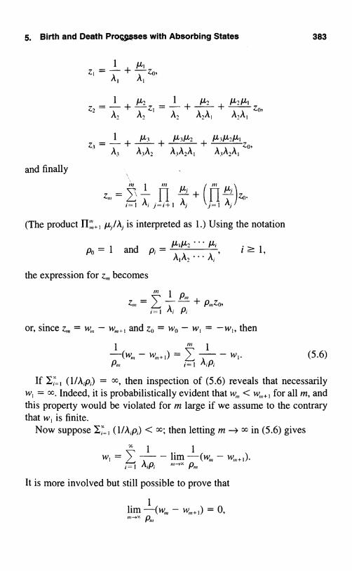
5. Birth and Death Proggses with Absorbing States
1 µ,Z, + Zo,
1 P, µ, µ,Itz, =
A, + A,Z,
A, + A,A + A, Z0'
1 + µ'3 + µ,µ,µizz3
A3 A3A, A,A,A, A3A,A, °'
and finally
(The product II;;;+, p,/A; is interpreted as 1.) Using the notation
1 and µ.µ_' µ`
the expression for z,,, becomes
Mm1 !_Z= + P,,,Zo,
r=1 i pi
or, since z,,, = is,, - w,,,+, and zo = wo - w, = -w,, then
1 "' 1
An j=1 ipi- VV'.
383
(5.6)
If G'i=, (1/A;p,) = oo, then inspection of (5.6) reveals that necessarilyw, = x. Indeed, it is probabilistically evident that w< w,,,+, for all m, andthis property would be violated for m large if we assume to the contrarythat w, is finite.
Now suppose I;_, (1/A;p;) < oo; then letting m - x in (5.6) gives
1 1- lim -(w- u;+.)j=1 A;P, An
It is more involved but still possible to prove that
1
lim -(w,,, - w,,,+,) = 0,

384 VI Continuous Time Markov Chains
and thenx
1
Aipi
We summarize the discussion of this section in the following theorem:
Theorem 5.1 Consider a birth and death process with birth and deathparameters A,, and p.,,, n ? 1, where A0 = 0 so that 0 is an absorbing state.
The probability of absorption into state 0 from the initial state m is
un =
=m Pim'1 + I;-, pi i=1
X
i=1
The mean time to absorption is
w
I k=1 j=k+1 AJpi
00i
i=
X
i=
1
Ai pi
- < ooAipi
(5.7)
(5.8)
where pa = 1 and p, = (µ1µ2 ... p'i)l(A1A2 ... Ai)
Example Population Processes Consider the linear growth birth anddeath process without immigration (cf. Section 3.3) for which µ = nµand A,, = nil, n = 0, 1..... During a short time interval of length h, a sin-gle individual in the population dies with probability µh + o(h) and givesbirth to a new individual with probability Ah + o(h), and thus µ > 0 andA > 0 represent the individual death and birth rates, respectively.
Substitution of a = 0 and i = m in equation (3.9) determines the meanpopulation size at time t for a population starting with X(0) = m individ-uals. This mean population size is M(t) = me' " 1, exhibiting exponentialgrowth or decay according as A > µ or A < A.
Let us now examine the extinction phenomenon and determine theprobability that the population eventually dies out. This phenomenon cor-responds to absorption in state 0 for the birth and death process.
When A,, = nA and µ = nµ, a direct calculation yields pi = (µ/ 1)i, andthen
00

5. Birth and Death Proses with Absorbing States
i =,n(µ/A)' = 1 - (A/A)
Co
when A > µ,
when A :5 A.
385
From Theorem 5.1, the probability of eventual extinction starting with mindividuals is
Pr{ExtinctionIX(0) = m} _ (µ"/A)n when A >µ.1 when A _ (5.9)
When A = µ, the process is sure to vanish eventually. Yet in this casethe mean population size remains constant at the initial population level.Similar situations where mean values do not adequately describe popula-tion behavior frequently arise when stochastic elements are present.
We turn attention to the mean time to extinction assuming that extinc-tion is certain, that is, when A A. For a population starting with a sin-gle individual, then, from (5.8) with m = 1 we determine this mean timeto be
1 _ 1i
1 I f xi_'dx
Ai=1o
x (A/µ)
(5.10)
Aipi A i 1 µ
Co
when
when

386 VI Continuous Time Markov Chains
When the birth rate A exceeds the death rate µ, a linear growth birth anddeath process can, with strictly positive probability, grow without limit. Incontrast, many natural populations exhibit density-dependent behaviorwherein the individual birth rates decrease or the individual death rates in-crease or both changes occur as the population grows. These changes areascribed to factors including limited food supplies, increased predation,crowding, and limited nesting sites. Accordingly, we introduce a notion ofenvironmental carrying capacity K, an upper bound that the populationsize cannot exceed.
Since all individuals have a chance of dying, with a finite carrying ca-pacity, all populations will eventually become extinct. Our measure ofpopulation fitness will be the mean time to extinction, and it is of interestto population ecologists studying colonization phenomena to examinehow the capacity K, the birth rate A, and the death rate µ affect this meanpopulation lifetime.
The model should have the properties of exponential growth (on the av-erage) for small populations, as well as the ceiling K beyond which thepopulation cannot grow. There are several ways of approaching the popu-lation size K and staying there at equilibrium. Since all such models givemore or less the same qualitative results, we stipulate the simplest model,in which the birth parameters are
nA forn=0,1,...,K- 1,"-I0 forn>K.
Theorem 5.1 yields w,, the mean time to population extinction startingwith a single individual, as given by
1 A A . . .A, , ;- I
i ArA, i== I !-'I/-k? ... At
1K
1 A
IL i\p(5.11)
Equation (5.11) isolates the distinct factors influencing the mean timeto population extinction. The first factor is 1/µ, the mean lifetime of an in-dividual, since µ is the individual death rate. Thus, the sum in (5.11) rep-resents the mean generations, or mean lifespans, to population extinction,a dimensionless quantity that we denote by
I
le, where 0 = . (5.12)-µ

5. Birth and Death Proc4gses with Absorbing States 387
Next we examine the influence of the birth-death, or reproduction, ratio0 = A/g and the carrying capacity K on the mean time to extinction. Since,1 represents the individual birth rate and 1/µ is the mean lifetime of a sin-gle member in the population, we may interpret the reproduction ratio0 = A(1/µ) as the mean number of offspring of an arbitrary individual inthe population. Accordingly, we might expect significantly different be-havior when 0 < 1 as opposed to when 0 > 1, and this is indeed the case.A carrying capacity of K = 100 is small. When K is on the order of 100or more, we have the following accurate approximations, their derivationsbeing sketched in Exercises 5.1 and 5.2:
Ms
for 0 < 1,
for 0 = 1, (5.13)
for 0 > 1.
The contrast between 0 < 1 and 0 > 1 is vivid. When 0 < 1, the meangenerations to extinction Mx is almost independent of carrying capacity Kand approaches the asymptotic value 0' ln(1 - 0)-' quite rapidly. When0 > 1, the mean generations to extinction Mg grows exponentially in K.Some calculations based on (5.13) are given in Table 5.1.
Table 5.1 Mean generations to extinction fora population starting with a singleparent and where 0 is the reproduc-tion rate and K is the environmen-tal capacity.
K 0=0.8 0= 1 0= 1.2
10 1.96 2.88 3.10100 2.01 5.18 4.14 x 1041000 2.01 7.48 7.59 x 1076

388 VI Continuous Time Markov Chains
Example Sterile Male Insect Control The screwworm fly, a cattlepest in warm climates, was eliminated from the southeastern United Statesby the release into the environment of sterilized adult male screwwormflies. When these males, artificially sterilized by radiation, mate with na-tive females, there are no offspring, and in this manner part of the repro-ductive capacity of the natural population is nullified by their presence. Ifthe sterile males are sufficiently plentiful so as to cause even a small de-cline in the population level, then this decline accelerates in succeedinggenerations even if the number of sterile males is maintained at approxi-mately the same level, because the ratio of sterile to fertile males will in-crease as the natural population drops. Because of this compounding ef-fect, if the sterile male control method works at all, it works to such anextent as to drive the native population to extinction in the area in whichit is applied.
Recently, a multibillion-dollar effort involving the sterile male tech-nique has been proposed for the control of the cotton boll weevil. In thisinstance, it was felt that pretreatment with a pesticide could reduce thenatural population size to a level such that the sterile male techniquewould become effective. Let us examine this assumption, first with a de-terministic model and then in a stochastic setting.
For both models we suppose that sexes are present in equal numbers,that sterile and fertile males are equally competitive, and that a constantnumber S of sterile males is present in each generation. In the determinis-tic case, if No fertile males are in the parent generation and the No fertilefemales choose mates equally likely from the entire male population, thenthe fraction No/(N0 + S) of these matings will be with fertile males andwill produce offspring. Letting 9 denote the number of male offspring thatresults from a fertile mating, we calculate the size N of the next genera-tion according to
N, = BNo(N+o S)
(5.14),,
For a numerical example, suppose that there are No = 100 fertile males(and an equal number of fertile females) in the parent generation of thenative population, and that S = 100 sterile male insects are released. If6 = 4, meaning that a fertile mating produces four males (and four fe-males) for the succeeding generation, then the number of both sexes in thefirst generation is
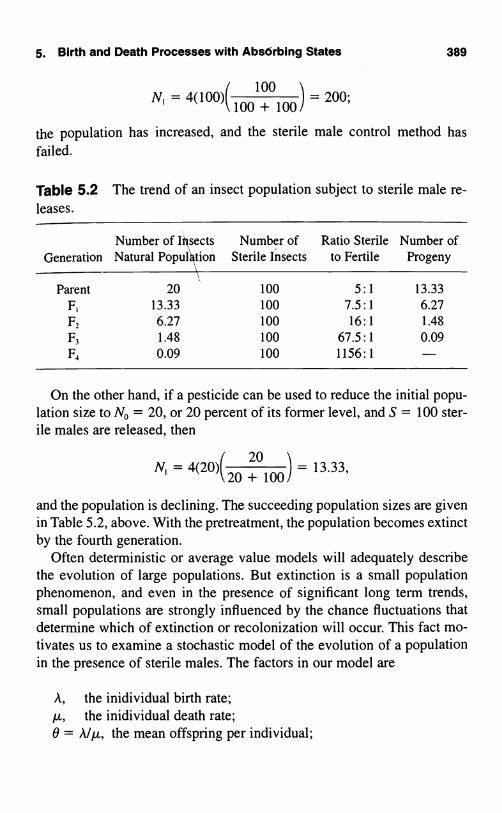
5. Birth and Death Processes with Absorbing States 389
N, = 4(100)(100100100) = 200;
the population has increased, and the sterile male control method hasfailed.
Table 5.2 The trend of an insect population subject to sterile male re-leases.
GenerationNumber of InsectsNatural Population
Number ofSterile Insects
Ratio Sterileto Fertile
Number ofProgeny
Parent 20 100 5:1 13.33F, 13.33 100 7.5:1 6.27
F, 6.27 100 16:1 1.48
F3 1.48 100 67.5:1 0.09F4 0.09 100 1156:1 -
On the other hand, if a pesticide can be used to reduce the initial popu-lation size to No = 20, or 20 percent of its former level, and S = 100 ster-ile males are released, then
and the population is declining. The succeeding population sizes are givenin Table 5.2, above. With the pretreatment, the population becomes extinctby the fourth generation.
Often deterministic or average value models will adequately describethe evolution of large populations. But extinction is a small populationphenomenon, and even in the presence of significant long term trends,small populations are strongly influenced by the chance fluctuations thatdetermine which of extinction or recolonization will occur. This fact mo-tivates us to examine a stochastic model of the evolution of a populationin the presence of sterile males. The factors in our model are
A, the inidividual birth rate;µ, the inidividual death rate;0 = AIA, the mean offspring per individual;

390 VI Continuous Time Markov Chains
K, the carrying capacity of the environment;S, the constant number of sterile males in the population;
in, the initial population size.
We assume that both sexes are present in equal numbers in the naturalpopulation and that X(t), the number of either sex present at time t,evolves as a birth and death process with parameters
A= fAn(n+S n<K,
0 forn?K,
and (5.15)
forn=0,1.....This is the colonization model of the Population Processes example,
modified in analogy with (5.14) by including in the birth rate the factorn/(n + S) to represent the probability that a given mating will be fertile.
To calculate the mean time to extinction w,,, as given in (5.8), we firstuse (5.15) to determine
P'_P" (µlk(k + S)!Pk =
A,A, Ak = \ A / k!S!
Po= 1, and pK=oo,or1/px=0,
and then substitute these expressions for pk into (5.8) to obtain
win =
In - I
fork= 1,...,K- 1,
In- 1 A
+A,P,
kL=1 ,-j=k+I A,P,
1In- I I-_
, k_=j=k+I AiPi k=O j=k+I IkiPi-'k j - =2 P (5.16)
1 1m-1 K-11 e,-k j!(S + k)1
µ O = j + 1 k!(S + j)!

S. Birth and Death Processes with Absorbing States 391
Because of the factorials, equation (5.16) presents numerical difficultieswhen direct computations are attempted. A simple iterative scheme worksto provide accurate and effective computation, however. We let
K-' j!(S + k)!
-k j + 1 k!(S + j)!'
so that w,,, _ (a. + + But it is easily verified that
ak_, = k + 0(S+ k )C".
Beginning with aK = 0, one successively computes aK_,, aK_21 ... , a0,and then w,,, = (a0 + + a,,,- )11.k.
Using this method, we have computed the mean generations to extinc-tion in the stochastic model for comparison with the deterministic modelas given in Table 5.2. Table 5.3 lists the mean generations to extinction forvarious initial population sizes m when K = S = 100, A = 4, and µ = 1,so that 0 = 4. Instead of the four generations to extinction as predicted bythe deterministic model when m = 20, we now estimate that the popula-tion will persist for over 8 billion generations!
Table 5.3 The mean lifespans toextinction in a birth anddeath model of a popula-tion containing a constantnumber S = 100 of sterilemales.
Initial Mean LifespansPopulation Size to Extinction
20 8,101,227,74810 4,306,5315 3,8224 566
3 65
2 6.3
1 1.2

392 VI Continuous Time Markov Chains
What is the explanation for the dramatic difference between the predic-tions of the deterministic model and the predictions of the stochasticmodel? The stochastic model allows the small but positive probability thatthe population will not die out but will recolonize and return to a higherlevel near the environmental capacity K, and then persist for an enormouslength of time.
While both models are qualitative, the practical implications cannot bedismissed. In any large-scale control effort, a wide range of habitats andmicroenvironments is bound to be encountered. The stochastic model sug-gests the likely possibility that some subpopulation in some pocket mightpersist and later recolonize the entire area. A sterile male program that de-pends on a pretreatment with an insecticide for its success is chancy atbest.
Exercises
5.1. Assuming 0 < 1, verify the following steps in the approximation toMg, the mean generation to extinction as given in (5.12):
K 1 K 6
Mg= -0 =e- fx;- ' dxi=1 1 i=1 0
fa1xK 'J dx 1 (e' x"=9 c 1_x dxB c 1-x-9c 1-xdx
e
In 1 -0-' fB 1-B
0
1 1 _ 1 OK+1OK+2
0 1-0 0\K+l +K+2+
= l In1 - 6K (I+K+Ie+K+102+...
0 1-0 K+I\ K+2 K+3 /
1 1OK
eln1-e (K+1)(1-9)

Problems 393
5.2. Assume that 0 > 1 and verify the following steps in the approxi-mation to Mg, the mean generation to extinction as given in (5.12):
j K-j+ 1 01l
+KI
I1+K`K11-1)2
_ OK- If 1 l_ OK
K L 1 - (1/0)J K(0 - 1)'
Problems
+KIOIKIJ1
5.1. Consider the sterile male control model as described in the exam-ple entitled "Sterile Male Insect Control" and let u,,, be the probability thatthe population becomes extinct before growing to size K starting withX(O) = m individuals. Show that
u = Pi form= 1,...,K,m K-Il1=o Pr
where
P1 = 0(S + i)!i.
5.2. Consider a birth and death process on the states 0, 1, ... , 5 withparameters
AO =N1o=As =N-5=0,
11, = 1, 1t2 = 2, A3 = 3, A4 - 4,
µ1=4, N2=3, µ3=2, µ= 1.

394 VI Continuous Time Markov Chains
Note that 0 and 5 are absorbing states. Suppose the process begins in stateX(0) = 2.
(a) What is the probability of eventual absorption in state 0?(b) What is the mean time to absorption?
6. Finite State Continuous Time Markov Chains
A continuous time Markov chain X(t) (t > 0) is a Markov process on thestates 0, 1, 2. .... We assume as usual that the transition probabilities arestationary; i.e.,
P,;(t) = Pr{X(t + s) = jjX(s) = i}. (6.1)
In this section we consider only the case where the state space S is finite,labeled as 10, 1, 2, . . . , N).
The Markov property asserts that P;;(t) satisfies
(a) P;(t) ? 0,
(b) P;(t) = 1, i, j = 0, 1, ... , N, andJ=O
(c) PA(s + t) = P;(s)Pjl(t) for t, s ? 0j=o
and we postulate in addition that
1, i=j,(d) lamP;(t)={0, ij.If P(t) denotes the matrix (;P;(t)
compactly in matrix notation as
(Chapman-Kolmogorov relation),
";_,, then property (c) can be written
P(t + s) = P(t)P(s), t, s ? 0. (6.2)
Property (d) asserts that P(t) is continuous at t = 0, since the fact P(O) = I(= identity matrix) is implied by (6.2). It follows simply from (6.2) thatP(t) is continuous for all t > 0. In fact, ifs = h > 0 in (6.2), then becauseof (d), we have

6. Finite State Continuou,ime Markov Chains 395
lim P(t + h) = P(t) lim P(h) = P(t)I = P(t). (6.3)
On the other hand, for t > 0 and 0 < h < t we write (6.2) in the form
P(t) = P(t - h)P(h). (6.4)
But P(h) is near the identity when h is sufficiently small, and so P(h)-'[the inverse of P(h)] exists and also approaches the identity I. Therefore,
P(t) = P(t) lim (P(h))-' = lim P(t - h). (6.5)
The limit relations (6.3) and (6.5) together show that P(t) is continuous.Actually, P(t) is not only continuous but also differentiable in that the
limits
1 -P;(h) -lim
h= q,
k-,0+
p;(h),1-,m
h = qi;, i 0 j,(6.6)
exist, where 0 < q,, < ° (i 0 j) and 0 :5- q; < oc. Starting with the relation
I - P,;(h),i=o,j*i
dividing by h, and letting h decrease to zero yields directly the relationN
q, = L, q,;.j=o,j*i
The rates q; and q;; furnish an infinitesimal description of the processwith
Pr{X(t + h) = jJX(t) = i} = q;;h + o(h) for i 0 j,
Pr{X(t + h) = it X(t) = i} = I - q;h + o(h).
In contrast to the infinitesimal description, the sojourn description ofthe process proceeds as follows: Starting in state i, the process sojournsthere for a duration that is exponentially distributed with parameter q;.The process then jumps to state j 0 i with probability p;, = q;;/q;; the so-journ time in state j is exponentially distributed with parameter q;, and so

396 VI Continuous Time Markov Chains
on. The sequence of states visited by the process, denoted by fo, 6......is a Markov chain with discrete parameter, called the embedded Markovchain. Conditioned on the state sequence o, .... , the successive so-journ times So, S ... are independent exponentially distributed randomvariables with parameters q,,,, qF , . . . , respectively.
Assuming that (6.6) has been verified, we now derive an explicit ex-pression for P;(t) in terms of the infinitesimal matrix
-qo q01 qON
qio -q1 INA=
NO qN i ... - qN
The limit relations (6.6) can be expressed concisely in matrix form:
limP(h) - I = A,
la-+0+ h(6.7)
which shows that A is the matrix derivative of P(t) at t = 0. Formally,A = P'(0).
With the aid of (6.7) and referring to (6.2), we have
P(t + h) - P(t) = P(t)[P(h) - I] = P(h) - IP(t). (6.8)
h h h
The limit on the right exists, and this leads to the matrix differential equa-tion
P'(t) = P(t)A = AP(t), (6.9)
where P(t) denotes the matrix whose elements are P'(t) = dP; (t)/dt. Theexistence of P'(t) is an obvious consequence of (6.7) and (6.8). The dif-ferential equations (6.9) under the initial condition P(0) = I can be solvedby standard methods to yield the formula
P(t)=eA,=I+If=
A" t"
n!(6.10)
Example The Two State Markov Chain Consider a Markov chain{X(t)} with states 10, 1) whose infinitesimal matrix is

6. Finite State Continuous Time Ma"rkov Chains
A=0
397
The process alternates between states 0 and 1. The sojourn times in state0 are independent and exponentially distributed with parameter a. Thosein state 1 are independent and exponentially distributed with parameter /3.We carry out the matrix multiplication
-a a
18-R
1 [-(a + /3)t]" Aa + n!
X-a a
R -R
= -(a + /3)-a a
R -R
to see that A2 = -(a + /3)A. Repeated multiplication by A then yields
which when inserted into (6.10) simplifies the sum according to
P(t)=I-
a2 + a/3 - a22 - a/3
-R2-a/3 /3222+a13
= I - a + R[e-("+")' - I IA
= I + 1 A - 1 Ae-l°+g".a+a+/3And with 7r = al(a + /i) and r = a + /3,
P(t) =1 - 7r 7r
1 - it IT
IT - 7r
-(1-IT) (1-IT)e-TI
which is the matrix expression for equations (3.14a-d).Returning to the general Markov chain on states (0, 1, ... , N), when
the chain is irreducible (all states communicate) then P; (t) > 0 for i,

398 VI Continuous Time Markov Chains
j = 0, 1, ... , N and lim,.. P;(t) = ir; > 0 exists independently of theinitial state i. The limiting distribution may be found by passing to thelimit in (6.9), noting that lim,,,. P'(t) = 0. The resulting equations for7 T = (?ro, ?T,, ... , ITN) are
- qo q01 . q0N
0 = 'nA = (ir0. ,7r1. . . . , 7TN)qio -qi q1N
qNo qN1
which is the same as
9N
qij, j=0,1,...,N. (6.11)i*j
Equation (6.11) together with
ITo + ITi + + ITN = 1 (6.12)
determines the limiting distribution.Equation (6.11) has a mass balance interpretation that aids us in under-
standing it. The left side TT;q; represents the long run rate at which parti-cles executing the Markov process leave state j. This rate must equal thelong run rate at which particles arrive at state j if equilibrium is to bemaintained. Such arriving particles must come from some state i * j, anda particle moves from state i 0 j to state j at rate q;;. Therefore, the rightside I.;#; 7rq;; represents the total rate of arriving particles.
Example Industrial Mobility and the Peter Principle Let us supposethat a draftsman position at a large engineering firm can be occupied by aworker at any of three levels: T = Trainee, J = Junior Draftsman, andS = Senior Draftsman. Let X(t) denote the level of the person in the posi-tion at time t, and suppose that X(t) evolves as a Markov chain whose in-finitesimal matrix is
T
A=JS

6. Finite State Continuous Time Markov Chains 399
Thus a Trainee stays at that rank for an exponentially distributed time hav-ing parameter aT and then becomes a Junior Draftsman. A Junior Drafts-man stays at that level for an exponentially distributed length of time hav-ing parameter a, = a,T + a,s. Then the Junior Draftsman leaves theposition and is replaced by a Trainee with probability a,T/a, or is promotedto a Senior Draftsman with probability a,/a,, and so on.
Alternatively, we may describe the model by specifying the movementsduring short time intervals according to
Pr{X(t + h) = JI X(t) = T} = aTh + o(h),
Pr{X(t + h) = TIX(t) = J} = a,Th + o(h),
Pr{X(t + h) = SIX(t) = J} = a,sh + o(h),
Pr{X(t+h)=TIX(t)=S}=ash+o(h),
and
Pr(X(t + h) = ijX(t) = i} = I - a;h + o(h) for i = T, J, S.
The equations for the equilibrium distribution (7T, ir,, 7TS) are, accord-ing to (6.11),
aJT7rJ + asIr ,
aJ,7T
1 = 7T + 7T, + 7T5,
and the solution is
a, a,IrT a,a, + a5a, + aTaJS'
asaT
J a,a, + a,aT +
aTa1s7r5 =
asa, + a,aT + aTa,s

400 VI Continuous Time Markov Chains
Let us consider a numerical example for comparison with an alternativemodel to be developed later. We suppose that the mean times in the threestates are
State Mean Time
T 0.1
J 0.2S 1.0
and that a Junior Draftsman leaves and is replaed by a Trainee with prob-ability s and is promoted to a Senior Draftsman with probability Thesesuppositions lead to the prescription aT =I 0, a,T = 2, a,s = 3, as = 1. Theequilibrium probabilities are
1(5) 5ITT =
1(5) + 1(10) + 10(3)=
45 =0.11,
.7r, =10 45= 0.22,
mss= 405 =0.67.
But the duration that people spend in any given position is not expo-nentially distributed in general. A bimodal distribution is often observedin which many people leave rather quickly, while others persist for a sub-stantial time. A possible explanation for this phenomenon is found in the"Peter Principle," which asserts that a worker is promoted until finallyreaching a position in which he or she is incompetent. When this happens,the worker stays in that job until retirement. Let us modify the industrialmobility model to accommodate the Peter Principle by considering twotypes of Junior Draftsmen, Competent and Incompetent. We suppose thata fraction p of Trainees are Competent, and q = 1 - p are Incompetent.We assume that a competent Junior Draftsman stays at that level for an ex-
2 Laurence J. and Raymond Hull, The Peter Principle, Buccaneer Books.Cutchogue, New York, 1969.
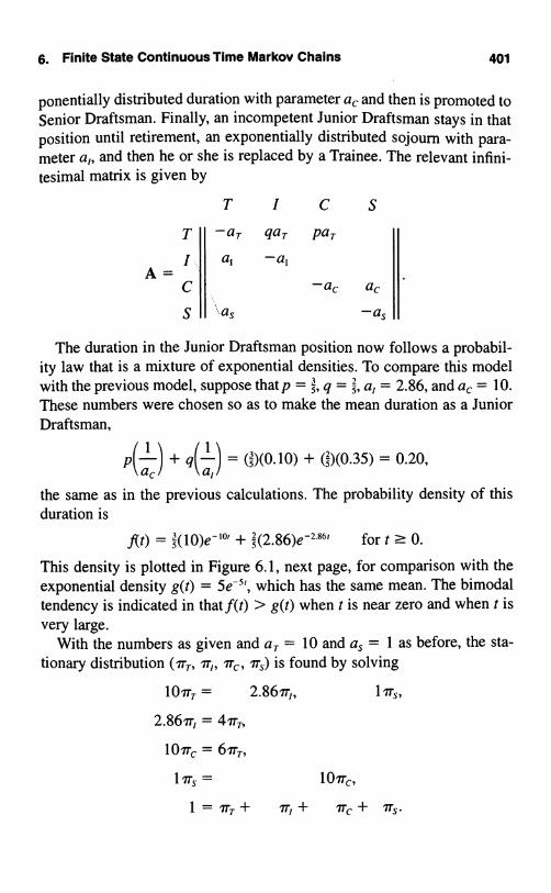
6. Finite State Continuous Time Markov Chains 401
ponentially distributed duration with parameter a, and then is promoted toSenior Draftsman. Finally, an incompetent Junior Draftsman stays in thatposition until retirement, an exponentially distributed sojourn with para-meter a,, and then he or she is replaced by a Trainee. The relevant infini-tesimal matrix is given by
T I C S
-ar qar paT
a, -a,
-ac ac
S -a,
The duration in the Junior Draftsman position now follows a probabil-ity law that is a mixture of exponential densities. To compare this modelwith the previous model, suppose that p = 3, q = 5, a, = 2.86, and ac = 10.These numbers were chosen so as to make the mean duration as a JuniorDraftsman,
PI 1) + ql 1 I = (3)(0.10) + (5)(0.35) = 0.20,\ a,a,the same as in the previous calculations. The probability density of thisduration is
f(t) = 3(10)e+ 5(2.86)e-z.aer for t ? 0.
This density is plotted in Figure 6.1, next page, for comparison with theexponential density g(t) = 5e 5r, which has the same mean. The bimodaltendency is indicated in thatf(t) > g(t) when t is near zero and when t isvery large.
With the numbers as given and ar = 10 and a, = I as before, the sta-tionary distribution (Irr, Tr irc, ir,) is found by solving
101rr = 2.86or,, 1 ar
2.861r, = 41Tr,
101rc = 61rr,
17r, = l0arc,
1 = Trr + Tr, + 7T + 7Ts.

402 VI Continuous Time Markov Chains
4.0
2.0
1.0
.60
.40
.20
.10
.06
.04
.02
0
1 1 1 1 I.2 .4 6 8 1.0
Figure 6.1 The exponential density (straight line) versus the mixed expo-nential density (curved line). Both distributions have the samemean. A logarithmic scale was used to accentuate the differences.
The solution is
7r,. = 0.111, ir, = 0.155,
ors = 0.667, 7r, = 0.067.
Let us make two observations before leaving this example. First, thelimiting probabilities 7r, , Tr and ir, = 'Ir, + Trc agree between the twomodels. This is a common occurrence in stochastic modeling, wherein thelimiting behavior of a process is rather insensitive to certain details of themodel and depends only on the first moments, or means. When this hap-pens, the model assumptions can be chosen for their mathematical conve-nience with no loss.
The second observation is specific to the Peter Principle. We have as-sumed that p = s of Trainees are competent Junior Draftsmen and onlyq = , are Incompetent. Yet in the long run, a Junior Draftsman is found tobe Incompetent with probability Mr,/(ar, + Ire) = 0.155/(0.155 + 0.067) _0.70!

6. Finite State Continuous Time Markov Chains 403
Example Redundancy and the Burn-In Phenomenon An airlinesreservation system has two computers, one on-line and one backup. Theoperating computer fails after an exponentially distributed duration hav-ing parameter µ and is replaced by the standby. There is one repair facil-ity, and repair times are exponentially distributed with parameter A. LetX(t) be the number of computers in operating condition at time t. ThenX(t) is a Markov chain whose infinitesimal matrix is
A=12
0 1 2
-(A + µ) A
ro
A 0
µ -µ
The stationary distribution (7ro, IT,, 7r,) satisfies
A7ro =
(A + µ)7r, = A7ro,
A1'2 =
and the solution is
7r,
IT,
A7r,,
1 = 1TO + 7r1 + 7T2,
1
1 + (Al p.) + (A µ)
Alµ1 + (A1µ) + (A/µ.)',
(Alp)21 + (Alµ) + (Alµ)'
The availability, or probability that at least one computer is operating, is1 -7rp=7T,+7r,.
Often in practice the assumption of exponentially distributed operatingtimes is not realistic because of the so-called burn-in phenomenon. Thisidea is best explained in terms of the hazard rate r(t) associated with aprobability density function f(t) of a nonnegative failure time T. Recall

404 Vi Continuous Time Markov Chains
that r(t) At measures the conditional probability that the item fails in thenext time interval (t, t + At) given that it has survived up to time t, andtherefore we have
r(t) = f (t) fort ? 0,1 - F(t)
where F(t) is the cumulative distribution function associated with theprobability density function f(t).
A constant hazard rate r(t) = A for all t corresponds to the exponentialdensity function f(t) = Ae-A' for t ? 0. The burn-in phenomenon is de-scribed by a hazard rate that is initially high and then decays to a constantlevel, where it persists, possibly later to rise again (aging). It correspondsto a situation in which a newly manufactured or newly repaired item hasa significant probability of failing early in its use. If the item survives thistest period, however, it then operates in an exponential or memorylessmanner. The early failures might correspond to incorrect manufacture orfaulty repair, or might be a property of the materials used.
Anyone familiar with automobile repairs has experienced the burn-inphenomenon.
One of many possible ways to model the burn-in phenomenon is to usea mixture of exponential densities
f(t) = pae' + q&-O', t ? 0, (6.13)
r(t)
2
1
0 0.2 0.4 0.6 0.8 t
Figure 6.2 The hazard rate corresponding to the density given in (6.13). Thehigher hazard rate at the initial t values represents the bum-inphenomenon.

Exercises 405
where 0 < p = 1 - q < 1 and a, /3 are positive. The density function forwhichp = 0.1, a = 10, q = 0.9, and 8 = 0.909 = 1/1.1 has mean one.Its hazard rate is plotted in Figure 6.2 on the previous page, where thehigher initial burn-in level is evident.
We may incorporate the burn-in phenomenon corresponding to themixed exponential density (6.13) by expanding the state space accordingto the following table:
Notation State
OA
1B
2A
28
Both computers downOne operating computer, current up time has parameter aOne operating computer, current up time has parameter /3Two operating computers, current up time has parameter aTwo operating computers, current up time has parameter /3
Equation (6.13) corresponds to a probability p that a computer begin-ning operation will have an exponentially distributed up time with para-meter a and a probability q that the parameter is /3. Accordingly, we havethe infinitesimal matrix
0 lA 1B 2A 2A
0 -A pA qA
lA a -(A + a) A
A = 18 /i -(A+/3) A
2A pa qa -a2Q p13 q13 -J6
The stationary distribution can be determined in the usual way by ap-plying (6.11).
Exercises
6.1. A certain type component has two states: 0 = OFF and 1 = OP-ERATING. In state 0, the process remains there a random length of time,which is exponentially distributed with parameter a, and then moves to
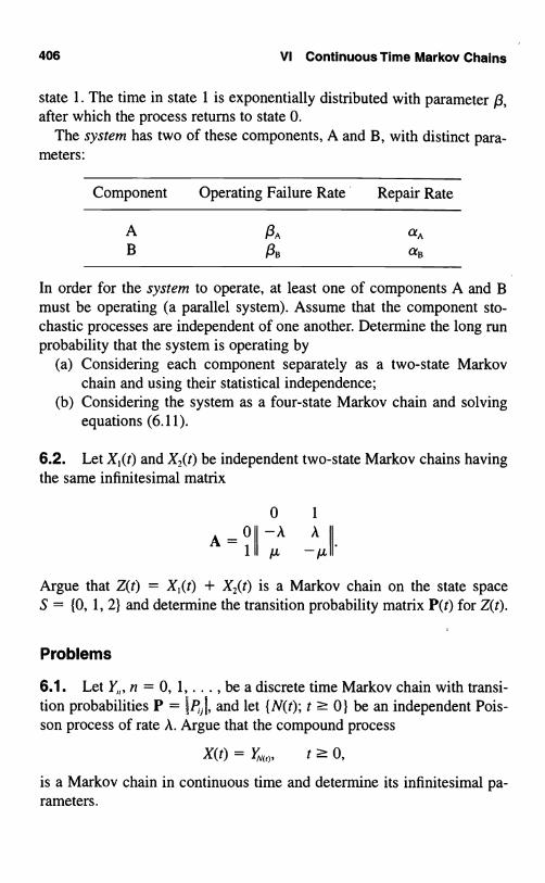
406 VI Continuous Time Markov Chains
state 1. The time in state 1 is exponentially distributed with parameter 13,after which the process returns to state 0.
The system has two of these components, A and B, with distinct para-meters:
Component Operating Failure Rate' Repair Rate
A NA aA
B 13B aB
In order for the system to operate, at least one of components A and Bmust be operating (a parallel system). Assume that the component sto-chastic processes are independent of one another. Determine the long runprobability that the system is operating by
(a) Considering each component separately as a two-state Markovchain and using their statistical independence;
(b) Considering the system as a four-state Markov chain and solvingequations (6.11).
6.2. Let X,(t) and X,(t) be independent two-state Markov chains havingthe same infinitesimal matrix
0 1
A =011 -A I1 µ µ jj_
Argue that Z(t) = X,(t) + XZ(t) is a Markov chain on the state spaceS = (0, 1, 2) and determine the transition probability matrix P(t) for Z(t).
Problems
6.1. Let Y,,, n = 0, 1, . . . , be a discrete time Markov chain with transi-tion probabilities P = lPA, and let {N(t); t ? 0) be an independent Pois-son process of rate A. Argue that the compound process
X(t) = Y,N(,), t ? 0,
is a Markov chain in continuous time and determine its infinitesimal pa-rameters.

Problems 407
6.2. A certain type component has two states: 0 = OFF and 1 =OPERATING. In state 0, the process remains there a random length oftime, which is exponentially distributed with parameter a, and then movesto state 1. The time in state 1 is exponentially distributed with parameterJ3, after which the process returns to state 0.
The system has three of these components, A, B, and C, with distinctparameters:
Component Operating Failure Rate Repair Rate
A 3A aA
B NB a6
C ac ac
In order for the system to operate, component A must be operating, and atleast one of components B and C must be operating. In the long run, whatfraction of time does the system operate? Assume that the component sto-chastic processes are independent of one another.
6.3. Let X, (t), X, (t), ... , XN(t) be independent two-state Markov chainshaving the same infinitesimal matrix
A=0
Determine the infinitesimal matrix for the Markov chain Z(t) _XI(t) + + XN(t).
6.4. A system consists of two units, both of which may operate simul-taneously, and a single repair facility. The probability that an operatingsystem will fail in a short time interval of length At is µ(4t) + o(Ot). Re-pair times are exponentially distributed, but the parameter depends onwhether the failure was regular or severe. The fraction of regular failuresis p, and the corresponding exponential parameter is a. The fraction of se-vere failure is q = 1 - p, and the exponential parameter is /3 < a.
Model the system as a continuous time Markov chain by taking asstates the pairs (x, y), where x = 0, 1, 2 is the number of units operating

408 VI Continuous Time Markov Chains
and y = 0, 1, 2 is the number of units undergoing repair for a severe fail-ure. The possible states are (2, 0), (1, 0), (1, 1), (0, 0), (0, 1), and (0, 2).Specify the infinitesimal matrix A. Assume that the units enter the repairshop on a first come, first served basis.
7. A Poisson Process with a Markov Intensity*
Consider "points" scattered in some manner along the semi-infinite inter-val [0, 00), and for an interval of the form I = (a, b], with 0 <_ a < b < cc,let N(1) count the number of "points" in the interval I. Then N(1), as Iranges over the half-open intervals I = (a, b], is a point process. (See V,Section 5 for generalizations to higher dimensions.) Suppose that, condi-tional on a given intensity, N(I) is a nonhomogeneous Poisson process,but where the intensity function (A(t), t ? 0) is itself a stochastic process.Such point processes were introduced in V, Section 1.4, where they werecalled Cox processes in honor of their discoverer. While Cox processesare sufficiently general to describe a plethora of phenomena, they remainsimple enough to permit explicit calculation, at least in some instances. Asan illustration, we will derive the probability of no points in an interval fora Cox process in which the intensity function is a two-state Markov chainin continuous time. The Cox process alternates between being "ON" and"OFF." When the underlying intensity is "ON," points occur according toa Poisson process of constant intensity A. When the underlying process is"OFF," no points occur. We will call this basic model a (0, A) Cox processto distinguish it from a later generalization. The (0, A) Cox process mightdescribe bursts of rainfall in a locale that alternates between dry spells andwet ones, or arrivals to a queue from a supplier that randomly shuts down.Rather straightforward extensions of the techniques that we will now usein this simple case can be adapted to cover more complex models andcomputations, as we will subsequently show.
We assume that the intensity process (A(t); t ? 0) is a two-state Markovchain in continuous time for which
Pr(A(t + h) = AIA(t) = 0) = ah + o(h), (7.1)
*Starred sections contain material of a more specialized or advanced nature.

7. A Poisson Process with a Markov Intensity 409
and
Pr{A(t + h) = OIA(t) = A) = /3h + o(h). (7.2)
This intensity is merely the constant A times the two-state birth and deathprocess of Section 3. As may be seen by allowing t - ° in (3.13), such aprocess has the limiting distribution Pr(A(c) = 0) = /3/(a + /3) andPr{A(°°) = A) = a/(a + /3). We will assume that the intensity process be-gins with this limiting distribution, or explicitly, that Pr(A(0) = 0) =/3/(a + /3) and Pr{A(0) A) = a/(a + (3). With this assumption, the in-tensity process is stationary in the sense that Pr{A(t) = 0) = /3/(a + /3)and Pr{A(t) = A] = a/(a +`,/3) for all t ? 0. This stationarity carries overto the Cox process N(I) to imply that Pr{N((0, t]) = k) = Pr{N((s, s + t])= k) for all s, t ? 0 and k = 0, 1..... We are interested in determining
f(t; A) = Pr{N((0, t]) = 0).
LetI
A(t) = f A(s) ds (7.3)0
and note the conditional Poisson probability
Pr {N((0, t]) = OIA(s) for s < t} = e
so that upon removing the conditioning via the law of total probability weobtain
At; A) = E[e-All)] = .f0(t) + f (t), (7.4)
where
fo(t) = Pr{N((0, t]) = 0 and A(t) = 0), (7.5)
and
fl(t) = Pr{N((0, t]) = 0 and A(t) = Al. (7.6)
Using an infinitesimal "last step analysis" similar to that used to derive theKolmogorov forward equations, we will derive a pair of first-order lineardifferential equations for fo(t) and f,(t). To this end, by analyzing the'pos-sibilities at time t and using the law of total probability, we begin with

410 VI Continuous Time Markov Chains
fo(t + h) =fa(t) Pr{N((t, t + h]) = OIA(t) = 0} Pr{A(t + h) = OIA(t) = 0)
+ fl(t) Pr{N((t, t + h]) = OJA(t) = A) Pr{A(t + h) = OIA(t) = A)
= fo(t)[1 - ah + o(h)] + f(t)e-A''/ih + o(h),
and
f(t+h)=fl(t) Pr{N((t, t + h]) = OIA(t) = A) Pr{A(t + h) = AIA(t) = A)
+ fo(t) Pr(N((t, t + h]) = OIA(t) = 01 Pr(A(t + h) = AJA(t) = 0)
= f,(t)e-A''[1 - /3h + o(h)] + fo(t)ah + o(h).
We rearrange the terms and use e-A" = 1 - Ah + o(h) to get
fo(t + h) - fo(t) = -afo(t)h + /3f,(t)h + o(h)
and
f, (t + h) - f, (t) = -(/3 + A)f,(t)h + afa(t)h + o(h),
which, after dividing by h and letting h tend to zero, become the differen-tial equations
dfo(t)dt
and
_ -afo(t) + f3ff(t) (7.7)
df, (t)
dt
The initial conditions are
= -(/3 + A)f (t) + af0(t). (7.8)
fo(0) = Pr(A(0) = 0) = /3/(a + /3) (7.9)
and
f(0) = Pr{A(0) = A} = a/(a + /3). (7.10)
Such coupled first-order linear differential equations are readily solved. Inour case, after carrying out the solution and simplifying the result, the an-swer is Pr{N((0, t]) = 0) = fo(t) + f(t) = f(t; A), where
f(t; A) = c+ exp{-µ+t} + c_ exp{-µ_t) (7.11)

7. A Poisson ProceM with a Markov Intensity 411
with
p =;{(A+a+/3)± (A+a+R)'-4aA}, (7.12)
[aA/(a + /3)] - µ_c+ =
and
µ+ - [aAI(a + /3)]c_ =
(7.13)
(7.14)
A Geheralization Let N be a Cox process driven by a 0-1 Markovchain A(t), but now suppose that when the intensity process is in state 0,the Cox process is, conditionally, a Poisson process of rate A0, and whenthe intensity process is in state 1, then the Cox process is a Poissonprocess of rate A,. The earlier Cox process had A. = 0 and A, = A. With-out loss of generality, we assume 0 < A. < A,.
In order to evaluate Pr{N((0, t]) = 01, we write N as the sum N =N, + N, of two independent processes, where N, is a Poisson process ofconstant rate A. and N, is a (0, A) Cox process with A = A, - A0. Then Nis zero if and only if both N, and N, are zero, whence
Pr{N((0, t]) = 0) = Pr{N,((0, t]) = t]) = 01
= e_Ao'f(t, A, - A0). (7.15)
Example The tensile strength S(t) of a single fiber of length t is oftenassumed to follow a Weibull distribution of the form
Pr{S(t) > x) = exp{-tox&}, for x > 0, (7.16)
where 6 and o are positive material constants. The explicit appearance ofthe length t in the exponent is an expression of a weakest-link size effect,in which the fiber strength is viewed as the minimum strength of inde-pendent sections. This theory suggests that the survivorship probability ofstrength for a fiber of length t should satisfy the relation
Pr{S(t) > x} = [Pr{S(1) > x}]', t > 0. (7.17)
The Weibull distribution is the only type of distribution that is concen-trated on 0 x < oo and satisfies (7.17).

412 VI Continuous Time Markov Chains
However, a fiber under stress may fail from a surface flaw such as anotch or scratch, or from an internal flaw such as a void or inclusion.Where the diameter d of the fiber varies along its length, the relative mag-nitude of these two types of flaws will also vary, since the surface of thefiber is proportional to d, while the volume is proportional to d 2. As a sim-ple generalization, suppose that the two types of flaws alternate and that thechanges from one flaw type to the other follow a two-state Markov chainalong the continuous length of the fiber. Further, suppose that a fiber ofconstant type i flaw, for i = 0, 1, will support the load x with probability
Pr(S(t) > x} = exp{-to;x% x > 0,
where o-; and S; are positive constants.We can evaluate the survivorship probability for the fiber having
Markov varying flaw types by bringing in an appropriate (A0, A,) Coxprocess. For a fixed x > 0, suppose that flaws that are weaker than x willoccur along a fiber of constant flaw type i according to a Poisson processof rate A,(x) = for i = 0, 1. A fiber of length t and having Markovvarying flaw types will carry a load of x if and only if there are no flawsweaker than x along the fiber. Accordingly, for the random flaw type fiber,using (7.15) we have
Pr(S(t) > x) = e-V'".f(t; 11,(x) - Ao(x)). (7.18)
Equation (7.18) may be evaluated numerically under a variety of as-sumptions for comparison with observed fiber tensile strengths. Wherefibers having two flaw types are tested at several lengths, (7.18) may beused to extrapolate and predict strengths at lengths not measured.
It is sometimes more meaningful to reparametrize according toit = a/(a + /3) and r = a + P. Here IT is the long run fraction of fiberlength for which the applicable flaw distribution is of type 1, and 1 - ITis the similar fraction of type 0 flaw behavior. The second parameter T isa measure of the rapidity with which the flaw types alternate. In particu-lar, when T = 0, the diameter or flaw type remains in whichever state itbegan, and the survivor probability reduces to the mixture
Pr{S(t) > x} = ire-",c' + (1 - (7.19)
On the other hand, at r = x, the flaw type process alternates instantly, andthe survivor probability simplifies to
Pr{S(t) > x} = exp{-t[irA,(x) + (1 - ir)Ao(x)]}. (7.20)

Exercises 413
The probability distribution for N((0, t]) Let A(t) be the cumula-tive intensity for a Cox process and suppose that we have evaluated
g(t; 0) = E[e-('-I)A("], 0 < 0 < 1.
For a (0, A) Cox process, for instance, g(t, 0) = f(t; (1 - 0)A), where f isdefined in (7.11). Upon expanding as a power series in 0, according to
g(t; 0) = E[e-A(')k=0
ek]k,A(t)'
-A(r)A(')k ] 0k
k!
Pr{N((0, t]) = k} ak,k=0
we see that the coefficient of 0k in the power series is Pr(N((0, t]) = k). Inprinciple then, the probability distribution for the points in an interval ina Cox process can be determined in any particular instance.
Exercises
7.1. Suppose that a (0, A) Cox process has a = /3 = 1 and A = 2. Showthat µ. = 2 ± \, and c_ =
;(2+ V) = 1 - c+, whence
Pr{N((0, t]) = 0) = e- 2 '[cosh(V2-t) + 2 sinh(\t)].
7.2. Suppose that a (0, A) Cox process has a = /3 = 1 and A = 2. Showthat
fO(t) =1 + V2_ + l - V Le-(2+N2),
4 4
and
f(t) = qe-(2-%2)r +4e-(2+)2)r
satisfy the differential equations (7.7) and (7.8) with the initial conditions(7.9) and (7.10).

414 VI Continuous Time Markov Chains
Problems
7.1. Consider a stationary Cox process driven by a two-state Markovchain. Let it = a/(a + 3) be the probability that the process begins instate A.
(a) By using the transition probabilities given in (3.14a-d), show thatPr{A(t) = A } = 7r for all t > 0.
(b) Show that E[N((O, t])] = TTAt for all t > 0.
7.2. The excess life y(t) in a point process is the random length of theduration from time t until the next event. Show that the cumulative distri-bution function for the excess life in a Cox process is given byPr{y(t) : x} = 1 - Pr{N((t, t + x]) = 0}.
7.3. Let T be the time to the first event in a stationary (0, A) Coxprocess. Find the probability density function 4)(t) for T. Show that whena = /3 = 1 and A = 2, this density function simplifies to ¢(t) = exp{ -2t}cosh(Vt).
7.4. Let T be the time to the first event in a stationary (0, A) Cox process.Find the expected value E[T]. Show that E[T] = 1 when a = 6 = 1 andA = 2. What is the average duration between events in this process?
7.5. Determine the conditional probability of no points in the interval(t, t + s], given that there are no points in the interval (0, t] for a station-ary Cox process driven by a two-state Markov chain. Establish the limit
lim Pr{N((t, t + s]) = 0IN((0, t]) = 0} = e-'"-5, s > 0.
7.6. Show that the Laplace transformx
(P(s; A) = f e-"f(t; A) dt0
is given by
=s+(1-ir)A+T
Cs; A) s2 + (T + A)s + 9TTA '

Problems 415
where T = a + /3 and IT = a/(a + /3). Evaluate the limit (a) as T -* 00,and (b) as T -3 0.
7.7. Consider a (0, A) stationary Cox process with a = /3 = 1 andA = 2. Show that g(t; 0) = f(t; (1 - 0)A) is given by
g(t; 0) = e-`--m' cosh(Rt) +1
Rsinh(Rt) ,
where
R = 0'-20+2.
Use this to evaluate Pr{N((0, 1]) = 11.
7.8. Consider a stationary (0, A) Cox process. A long duration duringwhich no events were observed would suggest that the intensity process isin state 0. Show that
Pr{A(t) = 0IN((0, t]) = 0) = fo(t)
.f(t) '
where fo(t) is defined in (7.5).
fo(t) = a+e--' + a_e_µ-'
f(t) = b+e-µ ' + b_e_µ-'
'(1 - IT)rl + (a+/3+A)jR= (a+ 9+A)2 4aAa.L R J
R J
satisfy the differential equations (7.7) and (7.8) subject to the initial con-ditions (7.9) and (7.10).

416 VI Continuous Time Markov Chains
7.10. Consider a stationary (0, A) Cox process.
(a) Show that
Pr{N((0, h]) > 0, N((h, h + t]) = 0) = f(t; A) - f(t + h; A),
whence
Pr{N((h h + t]) = 0IN((0 h]) > 01 =f(t; A) - f(t + h; A)
' 1 - f(h; A)
(b) Establish the limit
lim Pr(N((h, h + t]) = 0IN((0, h]) > 0) f '(t; A)=
-1011 f'(0, A)'
where
_ dftt; A)dt
(c) We interpret the limit in (b) as the conditional probability
Pr (N((O, t]) = 01 Event occurs at time 0).
Show that
Pr{N((0, t]) = 01 Event at time 01 = p+e-K+' + p_e-,U-',
where
C+µ+ c-M--p+ =
c+µ+ + c-µ-' p- = e+µ+ +c-lk-
(d) Let The the time to the first event in (0, c) in a stationary (0, A) Coxprocess with a = /3 = 1 and A = 2. Show that
E[rIEvent at time 0] = 1.
Why does this differ from the result in Problem 7.4?
7.11. A Stop-and-Go Traveler The velocity V(t) of a stop-and-go trav-eler is described by a two-state Markov chain. The successive durations inwhich the traveler is stopped are independent and exponentially distrib-uted with parameter a, and they alternate with independent exponentially

Problems 417
distributed sojourns, parameter /3, during which the traveler moves at unitspeed. Take the stationary case in which Pr{V(0) = 1) = Tr = a/(a + /3).The distance traveled in time t is the integral of the velocity:
I
S(t) = J V(u) du.
Show that0
E[e "(')] = f(t; 0), 0 real.
(This is the Laplace transform of the probability density function of S(t).)
7.12. 'Let T be the time of the first event in a (O, A) Cox process. Let the0 and A states represent "OFF" and "ON," respectively.
(a) Show that the total duration in the (0, T] interval that the system isON is exponentially distributed with parameter A and does not de-pend on a, f3 or the starting state.
(b) Assume that the process begins in the OFF state. Show that the totalduration in the (0, T] interval that the system is OFF has the samedistribution as
where is exponentially distributed with parameter A, N(t) is a Poissonprocess with parameter /3, and qo, -q,, ... are independent and exponen-tially distributed with parameter a.


Chapter VIIRenewal Phenomena
1. Definition of a Renewal Processand Related Concepts
Renewal theory began with the study of stochastic systems whose evolu-tion through time was interspersed with renewals or regeneration timeswhen, in a statistical sense, the process began anew. Today, the subject isviewed as the study of general functions of independent, identically dis-tributed, nonnegative random variables representing the successive inter-vals between renewals. The results are applicable in a wide variety of boththeoretical and practical probability models.
A renewal (counting) process {N(t), t > 0} is a nonnegative integer-valued stochastic process that registers the successive occurrences of anevent during the time interval (0, t], where the times between consecutiveevents are positive, independent, identically distributed random variables.Let the successive durations between events be {Xk}A , (often representingthe lifetimes of some units successively placed into service) such that X;is the elapsed time from the (i - 1)st event until the occurrence of the ithevent. We write
F(x)=Pr{Xksx}, k= 1,2,3,...,

420 VII Renewal Phenomena
for the common probability distribution of X X2..... A basic stipulationfor renewal processes is F(O) = 0, signifying that X,, X,, ... are positiverandom variables. We refer to
n?1
(W0 = 0 by convention),
as the waiting time until the occurrence of the nth event.The relation between the interoccurrence times {Xk} and the renewal
counting process {N(t), t ? 0) is depicted in Figure 1.1. Note formally that
N(t) = number of indices n for which 0 < W :5 t.
N(t)
X 1 -010 X, -0 -X3 {
WO W, W, W3
t
Figure 1.1 The relation between the interoccurrence times Xk and therenewal counting process N(t).
(1.2)
In common practice the counting process {N(t), t ? 0) and the partialsum process { W,,, n ? 0) are interchangeably called the "renewalprocess." The prototypical renewal model involves successive replace-ments of light bulbs. A bulb is installed for service at time WO = 0, fails attime W, = X,, and is then exchanged for a fresh bulb. The second bulbfails at time W, = X, + X, and is replaced by a third bulb. In general, thenth bulb burns out at time W = X, + + X and is immediately re-placed, and the process continues. It is natural to assume that the succes-sive lifetimes are statistically independent, with probabilistically identical
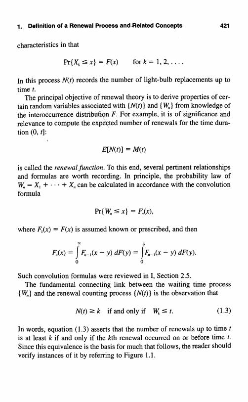
1. Definition of a Renewal Process and-Related Concepts 421
characteristics in that
Pr{XA : x} = F(x) for k = 1, 2, ... .
In this process N(t) records the number of light-bulb replacements up totime t.
The principal objective of renewal theory is to derive properties of cer-tain random variables associated with { N(t) } and { W,,) from knowledge ofthe interoccurrence distribution F. For example, it is of significance andrelevance to compute the expected number of renewals for the time dura-tion (0, t]:
E[N(t)] = M(t)
is called the renewal function. To this end, several pertinent relationshipsand formulas are worth recording. In principle, the probability law ofW = X, + + X,, can be calculated in accordance with the convolutionformula
Pr{ W <_ x} =
where F,(x) = F(x) is assumed known or prescribed, and then
x X
F,,(x) = f y) dF(y) = fF,,-,(x - y) dF(y).0 0
Such convolution formulas were reviewed in I, Section 2.5.The fundamental connecting link between the waiting time process
{ W,} and the renewal counting process {N(t)} is the observation that
N(t) ? k if and only if W t. (1.3)
In words, equation (1.3) asserts that the number of renewals up to time tis at least k if and only if the kth renewal occurred on or before time t.Since this equivalence is the basis for much that follows, the reader shouldverify instances of it by referring to Figure I.I.

422 VII Renewal Phenomena
It follows from (1.3) that
Pr{N(t)? k) =Pr(Wkst}=Fk(t), t?O,k= 1,2,..., (1.4)
and consequently,
Pr{N(t) = k} = Pr{N(t) ? k} - Pr (N(t) ? k + 1 }
Fk(t)-Fk+I(t), t?O,k= 1,2,.... (1.5)
For the renewal function M(t) = E[N(t)] we sum the tail probabilities inthe manner E[N(t)] Ek., Pr{N(t) ? k}, as derived in I, (5.2), and thenuse (1.4) to obtain
xM(t) = E[N(t)] = 7, Pr{N(t) ? k}
k=1
Pr{Wkst} F(t). (1.6)k=1 k=1
There are a number of other random variables of interest in renewaltheory. Three of these are the excess life (also called the excess randomvariable), the current life (also called the age random variable), and thetotal life, defined, respectively, by
y, = WN(6)+I - t (excess or residual lifetime),
6, = t - WN(,) (current life or age random variable),
/3, = y, + 6, (total life).
A pictorial description of these random variables is given in Figure 1.2.
N(t)
WO t
,
'Y,
WN(,) + I t
Figure 1.2 The excess life y,, the current life S and the total life 0,.

1. Definition of a Renewal Process and Related Concepts 423
An important identity enables us to evaluate the mean of in termsof the mean lifetime µ = E[X,] of each unit and the renewal functionM(t). Namely, it is true for every renewal process that
E[Wv(n+i] = E[X, + ... + X,v(,)+i]
= E[X,]{E[N(t) + 1]},
or
{M(t) + 1). (1.7)
At first glance, this identity resembles the formula given in II, (3.9) for themean of a random sum, which asserts that E[X, + + X,,,] = E[X,]E[N]when N is an integer-valued random variable that is independent of X,X,..... The random sum approach does not apply in the current context,however, the crucial difference being that the random number of sum-mands N(t) + 1 is not independent of the summands themselves. Indeed,in Section 3, on the Poisson process viewed as a renewal process, we willshow that the last summand X,N,,,+, has a mean that approaches twice theunconditional mean µ = E[X,] for t large. For this reason, it is not correct,in particular, that E[W,v,,,,] can be evaluated as the product of E[X,] andE[N(t)]. In view of these comments, the identity expressed in equation(1.7) becomes more intriguing and remarkable.
To derive (1.7), we will use the fundamental equivalence (1.3) in theform
N(t)?j- 1 if and only if t,
which expressed in terms of indicator random variables becomes
1{N(t)?j- 1} =1{X, +- +X,_,:5 t}.
Since this indicator random variable is a function only of the random vari-ables X ... , X;_ , it is independent of X,, and thus we may evaluate
t}]
(1.8)
µF-1(t).
With (1.8) in hand, the evaluation of the equivalence expressed in (1.7)

424 VII Renewal Phenomena
becomes straightforward. We have
E[WN(,)+l] = E[X, + ... + 40+i]
IN(t)+I 11
= E[X,] + EL 7, Xi]j=2
µ+E[ >X;1{N(t)+ 1?jLJ-2
i=2
= µ + µ F_#) (using (1.8))i=2
= µ[ 1 + M(t)] (using (1.6)).
Some examples of the use of the identity (1.7) will appear in the exercises,and an alternative proof in the case of a discrete renewal process can befound in Section 6.
Exercises
1.1. Verify the following equivalences for the age and the excess life ina renewal process N(t):
y, > x if and only if N(t + x) - N(t) = 0;
and for 0 < x < t,
S,>x if and only if N(t)-N(t-x)=0.Why is the condition x < t important in the second case but not the first?
1.2. Consider a renewal process in which the interoccurrence timeshave an exponential distribution with parameter A:
f(x) = Ae-', and F(x) = 1 - e-a" for x > 0.
Calculate F(t) by carrying out the appropriate convolution [see theequation just prior to (1.3)] and then determine Pr(N(t) = 1 } from equa-tion (1.5).
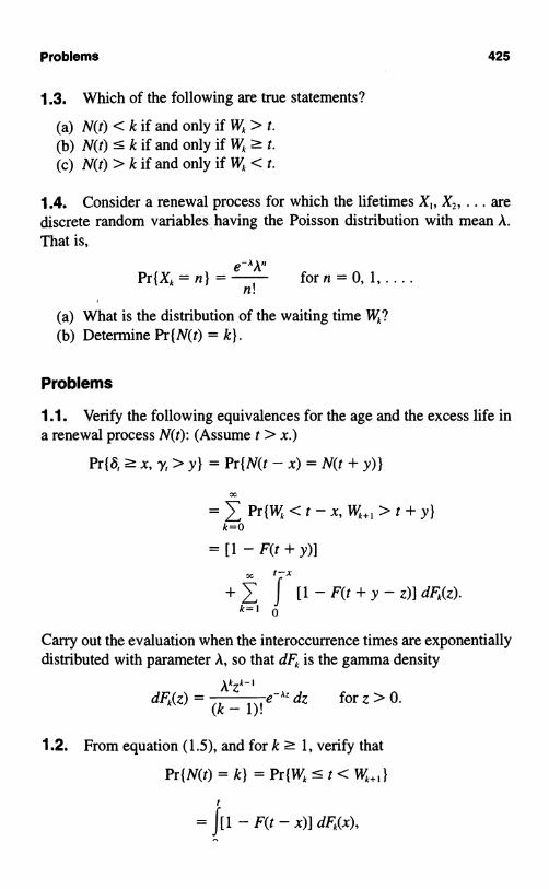
Problems 425
1.3. Which of the following are true statements?
(a) N(t) < k if and only if Wk > t.(b) N(t) :5 k if and only if W4. ?t.(c) N(t) > k if and only if Wk < t.
1.4. Consider a renewal process for which the lifetimes X,, X,, ... arediscrete random variables having the Poisson distribution with mean A.That is,
e-AnPr{Xk=n}_ A forn=0,1,....
n!
(a) What is the distribution of the waiting time Wk?(b) Determine Pr{N(t) = k).
Problems
1.1. Verify the following equivalences for the age and the excess life ina renewal process N(t): (Assume t > x.)
Pr{S,?x,y,>y} =Pr{N(t-x)=N(t+y)}
k=0Pr{Wk<t-x,Wk+i>t+y}
=[1-F(t+y)]t-x
+ f [I - F(t + y - z)] dFk(z).k=1 0
Carry out the evaluation when the interoccurrence times are exponentiallydistributed with parameter A, so that dFk is the gamma density
Akzk-1
dFk(z) =(k 1)!
e AZ dz for z > 0.-1.2. From equation (1.5), and for k ? 1, verify that
Pr{N(t)=k} =Pr{Wk:t<Wk+,}
= J[1 - F(t - x)] dFk(x),

426 VII Renewal Phenomena
and carry out the evaluation when the interoccurrence times are exponen-tially distributed with parameter A, so that dFk is the gamma density
AkZk-i
dFA(z) = (k _ 1) e A= dz for z > 0.
1.3. A fundamental identity involving the renewal function, valid for allrenewal processes, is
E[Wv(,,+i] = E[X1](M(t) + 1).
See equation (1.7). Using this identity, show that the mean excess life canbe evaluated in terms of the renewal function via the relation
E[y] = E[X,](1 + M(t)) - t.
1.4. Let y, be the excess life and S, the age in a renewal process havinginteroccurrence distribution function F(x). Determine the conditionalprobability Pr{ y, > yes, = x} and the conditional mean E[y,IS, = x].
2. Some Examples of Renewal Processes
Stochastic models often contain random times at which they, or some partof them, begin afresh in a statistical sense. These renewal instants formnatural embedded renewal processes, and they are found in many diversefields of applied probability including branching processes, insurance riskmodels, phenomena of population growth, evolutionary genetic mecha-nisms, engineering systems, and econometric structures. When a renewalprocess is discovered embedded within a model, the powerful results ofrenewal theory become available for deducing implications.
2.1. Brief Sketches of Renewal Situations
The synopses that follow suggest the wide scope and diverse contexts inwhich renewal processes arise. Several of the examples will be studied inmore detail in later sections.
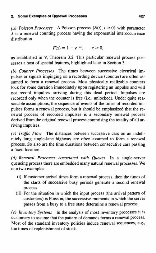
2. Some Examples of Fnewal Processes 427
(a) Poisson Processes A Poisson process (N(t), t ? 01 with parameterA is a renewal counting process having the exponential interoccurrencedistribution
F(x) = I - e-', x ? 0,
as established in V, Theorem 3.2. This particular renewal process pos-sesses a host of special features, highlighted later in Section 3.
(b) Counter Processes The times between successive electrical im-pulses or signals impinging on a recording device (counter) are often as-sumed to form a renewal process. Most physically realizable counterslock for some duration immediately upon registering an impulse and willnot record impulses arriving during this dead period. Impulses arerecorded only when the counter is free (i.e., unlocked). Under quite rea-sonable assumptions, the sequence of events of the times of recorded im-pulses forms a renewal process, but it should be emphasized that the re-newal process of recorded impulses is a secondary renewal processderived from the original renewal process comprising the totality of all ar-riving impulses.
(c) Traffic Flow The distances between successive cars on an indefi-nitely long single-lane highway are often assumed to form a renewalprocess. So also are the time durations between consecutive cars passinga fixed location.
(d) Renewal Processes Associated with Queues In a single-serverqueueing process there are embedded many natural renewal processes. Wecite two examples:
(i) If customer arrival times form a renewal process, then the times ofthe starts of successive busy periods generate a second renewalprocess.
(ii) For the situation in which the input process (the arrival pattern ofcustomers) is Poisson, the successive moments in which the serverpasses from a busy to a free state determine a renewal process.
(e) Inventory Systems In the analysis of most inventory processes it iscustomary to assume that the pattern of demands forms a renewal process.Most of the standard inventory policies induce renewal sequences, e.g.,the times of replenishment of stock.
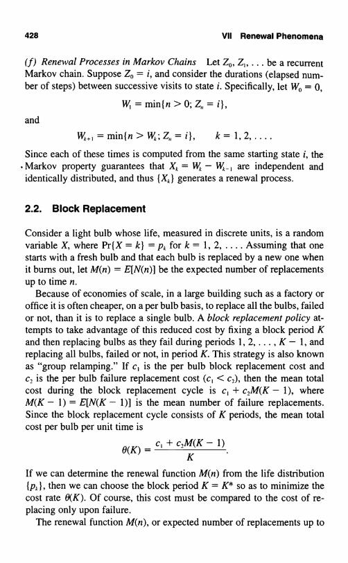
428 VII Renewal Phenomena
(f) Renewal Processes in Markov Chains Let Z0, Z,, . . . be a recurrentMarkov chain. Suppose Z = i, and consider the durations (elapsed num-ber of steps) between successive visits to state i. Specifically, let W,, = 0,
W,=min[ n>O;Z,, =i},and
W+, =min{n>W;Z,, =i}, k= 1,2.....Since each of these times is computed from the same starting state i, theMarkov property guarantees that Xk = W - W,, are independent andidentically distributed, and thus {XA} generates a renewal process.
2.2. Block Replacement
Consider a light bulb whose life, measured in discrete units, is a randomvariable X, where Pr{X = k} = p, for k = 1, 2, .... Assuming that onestarts with a fresh bulb and that each bulb is replaced by a new one whenit burns out, let M(n) = E[N(n)] be the expected number of replacementsup to time n.
Because of economies of scale, in a large building such as a factory oroffice it is often cheaper, on a per bulb basis, to replace all the bulbs, failedor not, than it is to replace a single bulb. A block replacement policy at-tempts to take advantage of this reduced cost by fixing a block period Kand then replacing bulbs as they fail during periods 1, 2, ... , K - 1, andreplacing all bulbs, failed or not, in period K. This strategy is also knownas "group relamping." If c, is the per bulb block replacement cost andc, is the per bulb failure replacement cost (c, < c,), then the mean totalcost during the block replacement cycle is c, + c,M(K - 1), whereM(K - 1) = E[N(K - 1)] is the mean number of failure replacements.Since the block replacement cycle consists of K periods, the mean totalcost per bulb per unit time is
0(K) = c, + c,M(K - 1)K
If we can determine the renewal function M(n) from the life distribution{ pj, then we can choose the block period K = K* so as to minimize thecost rate 0(K). Of course, this cost must be compared to the cost of re-placing only upon failure.
The renewal function M(n), or expected number of replacements up to

2. Some Examples of Renewal Processes 429
time n, solves the equationI
M(n) = FX(n) + pkM(n - k) for n = 1, 2, ... .k=I
To derive this equation, condition on the life X, of the first bulb. If it failsafter time n, there are no replacements during periods [1, 2, ... , n]. Onthe other hand, if it fails at time k < n, then we have its failure plus, onthe average, M(n - k) additional replacements during the interval [k + 1,k + 2, ... , n]. Using the law of total probability to sum these contribu-tions, we obtain
x n
M(n) = pk(0) + L pk[ 1 + M(n - k)]k=n+1 k=1
n-I
= FX(n) + 7, pkM(n - k) [because M(0) = 0],k=1
as asserted.
Thus we determine
M(1) = FX(1),
M(2) = FX(2) + p,M(1),
M(3) = FX(3) + p,M(2) + p,M(1),
and so on.To consider a numerical example, suppose that
p, = 0.1, p2 = 0.4, p, = 0.3, and p4 = 0.2,
and
Then
c,=2 and c,=3.
M(1) = p, = 0.1,
M(2)=(p,+P2)+p,M(1)=(0.1 +0.4)+0.1(0.1)=0.51,
M(3)=(p, +p2+p,)+p,M(2)+p2M(1)
= (0.1 +0.4+0.3)+0.1(0.51)+0.4(0.1)=0.891,
M(4)=(p, +p2+p,+ p4)+p,M(3)+p,M(2)+p,M(l)
= 1 + 0.1(0.891) + 0.4(0.51) + 0.3(0.1) = 1.3231.

430 VII Renewal Phenomena
The average costs are shown in the following table:
dBl k P i C1+ c,M(K - 1)
C =eroc o ost K = 0(K)K
1 2.000002 1.150003 1.176674 1.168255 1.19386
The minimum cost block period is K* = 2.We wish to elicit one more insight from this example. Forgetting about
block replacement, we continue to calculate
M(5) = 1.6617,
M(6) = 2.0647,
M(7) = 2.4463,
M(8) = 2.8336,
M(9) = 3.2136,
M(10) = 3.6016.
Let u,, be the probability that a replacement occurs in period n. Then M(n)= M(n - 1) + u asserts that the mean replacements up to time n is themean replacements up to time n - 1 plus the probability that a replacementoccurs in period n. The calculations are shown in the following table:
n u,, = M(n) - M(n - 1)
1 0.10002 0.41003 0.38104 0.43215 0.33866 0.40307 0.38168 0.38739 0.3800
10 0.3880
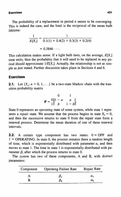
Exercises 431
The probability of a replacement in period n seems to be converging.This is indeed the case, and the limit is the reciprocal of the mean bulblifetime:
1 _ 1
E[X,] 0.1(1) + 0.4(2) + 0.3(3) + 0.2(4)
This calculation makes sense. If a light bulb lasts, on the average, E[X,]time units, then the probability that it will need to be replaced in any pe-riod should approximate 1/E[X,]. Actually, the relationship is not as sim-ple as just stated. Further discussion takes place in Sections 4 and 6.
Exercises
2.1. Let {X,,; n = 0, 1, ...) be a two-state Markov chain with the tran-sition probability matrix
P=00 1
l-a ab 1 -b'
State 0 represents an operating state of some system, while state 1 repre-sents a repair state. We assume that the process begins in state X0 = 0,and then the successive returns to state 0 from the repair state form arenewal process. Determine the mean duration of one of these renewalintervals.
2.2. A certain type component has two states: 0 = OFF and1 = OPERATING. In state 0, the process remains there a random lengthof time, which is exponentially distributed with parameter a, and thenmoves to state 1. The time in state 1 is exponentially distributed with pa-rameter 0, after which the process returns to state 0.
The system has two of these components, A and B, with distinctparameters:
Component Operating Failure Rate Repair Rate
A Al a,B Nf3 aR

432 VII Renewal Phenomena
In order for the system to operate, at least one of components A and Bmust be operating (a parallel system). Assume that the component sto-chastic processes are independent of one another. Consider the successiveinstants that the system enters the failed state from an operating state. Usethe memoryless property of the exponential distribution to argue that theseinstants form a renewal process.
2.3. Calculate the mean number of renewals M(n) = E[N(n)] for the re-newal process having interoccurrence distribution
for n = 1, 2, ... , 10. Also calculate u = M(n) - M(n - 1).
Problems
2.1. For the block replacement example of this section for whichp, = 0.1, P2 = 0.4, p3 = 0.3, and p, = 0.2, suppose the costs are c, = 4and c2 = 5. Determine the minimal cost block period K* and the cost ofreplacing upon failure alone.
2.2. Let X,, X2, ... be the interoccurrence times in a renewal process.Suppose Pr(Xk = 1) = p and Pr{Xk = 2} = q = 1 - p. Verify that
M(n) = E[N(n)] =n - qz
r l - ( q) ]1 + q (1 + q)2
forn=2,4,6.....
2.3. Determine M(n) when the interoccurrence times have the geo-metric distribution
Pr{X,=k)=pk=(3(l-I3) k-' fork=1,2,...,where 0</3< 1.
3. The Poisson Process Viewed as a Renewal Process
As mentioned earlier, the Poisson process with parameter A is a renewalprocess whose interoccurrence times have the exponential distributionF(x) = 1 - e-', x ? 0. The memoryless property of the exponential dis-

3. The Poisson Process Viewed as a Renewal Process 433
tribution (see Sections 4.2, 5.2 of I, and V) serves decisively in yieldingthe explicit computation of a number of functionals of the Poisson re-newal process.
The Renewal Function Since N(t) has a Poisson distribution, then(At)ke-rt
Pr{N(t)=k] ki , k=0,1,...,
and
M(t) = E[N(t)] = At.
Excess Life Observe that the excess life at time t exceeds x if and onlyif there are no renewals in the interval (t, t + x] (Figure 3.1). This eventhas the same probability as that of no renewals in the interval (0, x], sincea Poisson process has stationary independent increments. In formal terms,we have
Pr{y, > x} = Pr{N(t + x) - N(t) = 0}(3.1)
= Pr(N(x) = 0) = e-'.
Thus, in a Poisson process, the excess life possesses the same exponentialdistribution
Pr{y, : x) = 1 - e-1, x ? 0, (3.2)
as every life, another manifestation of the memoryless property of the ex-ponential distribution.
N(t)
t t+x
Figure 3.1 The excess life y, exceeds x if and only if there are no renewalsin the interval (t, t + x].

434 VII Renewal Phenomena
Current Life The current life S of course, cannot exceed t, while forx < t the current life exceeds x if and only if there are no renewals in(t - x, t], which again has probability e". Thus the current life followsthe truncated exponential distribution
Pr Ifor0<x<t,
= ){ o, < x }1 for t s x. (3.3
Mean Total Life Using the evaluation of I, (5.3) for the mean of a non-- negative random variable, we have
E[t3,] = E[y,] + E[8,]
= +JPr{S,>x}dx0
.+ Jedx0
= I + I (I - e-a,).
Observe that the mean total life is significantly larger than the mean life1/A = E[Xk] of any particular renewal interval. A more striking expressionof this phenomenon is revealed when t is large, where the process hasbeen in operation for a long duration. Then the mean total life E[/3,] is ap-proximately twice the mean life. These facts appear at first paradoxical.
Let us reexamine the definition of the total life /3, with a view to ex-plaining on an intuitive basis the seeming discrepancy. First, an arbitrarytime point t is fixed. Then /3, measures the length of the renewal intervalcontaining the point t. Such a procedure will tend with higher likelihoodto favor a lengthy renewal interval rather than one of short duration. Thephenomenon is known as length-biased sampling and occurs, well dis-guised, in a number of sampling situations.
Joint Distribution of y, and St The joint distribution of y, and S, isdetermined in the same manner as the marginals. In fact, for any x > 0 and0 < y < t, the event { y, > x, 5, > y) occurs if and only if there are no re-newals in the interval (t - y, t + x], which has probability e-A``+`". Thus

Problems 435
{e_MY) ifx>0,0<y<Pr{y,>x, S,>y} =
0 ify>t. (3.4)
For the Poisson process, observe that y, and S, are independent, since theirjoint distribution factors as the product of their marginal distributions.
Exercises
3.1. Let W,, W,, ... be the event times in a Poisson process (X(t); t ? 0)of rate A. Evaluate
Pr{WN(,)+, > t + s} and E[WN(,)+I]
3.2. Particles arrive at a counter according to a Poisson process of rateA. An arriving particle is recorded with probability p and lost with proba-bility 1 - p independently of the other particles. Show that the sequenceof recorded particles is a Poisson process of rate Ap.
3.3. Let W,, W,, ... be the event times in a Poisson process (N(t); t ? 0)of rate A. Show that
N(t) and WN(,)+I
are independent random variables by evaluating
Pr{N(t) = n and WN(,)+, > t + s).
Problems
3.1. In another form of sum quota sampling (see V, Section 4.2), a se-quence of nonnegative independent and identically distributed randomvariables X XZ, ... is observed, the sampling continuing until the firsttime that the sum of the observations exceeds the quota t. In renewalprocess terminology, the sample size is N(t) + 1. The sample mean is
WN(,)+I X, + . . . + VN(,)+I
N(t) + 1 N(t) + 1
An important question in statistical theory is whether or not this samplemean is unbiased. That is, how does the expected value of this sample

436 VII Renewal Phenomena
mean relate to the expected value of, say, X,? Assume that the individualX summands are exponentially distributed with parameter A, so that N(t)is a Poisson process, and evaluate the expected value of the foregoingsample mean and show that
Wv(n+, 1lEN(t)+1 =-L[1
Hint: Use the result of the previous exercise, that
WN(,)+, and N(t)
are independent, and then evaluate separately
E[WNU,+,I and E( 1
L N(t) + 1
3.2. A fundamental identity involving the renewal function, valid for allrenewal processes, is
E[%(,)+1] = E[X,](M(t) + 1).
See equation (1.7). Evaluate the left side and verify the identity when therenewal counting process is a Poisson process.
3.3. Pulses arrive at a counter according to a Poisson process of rate A.All physically realizable counters are imperfect, incapable of detecting allsignals that enter their detection chambers. After a particle or signal ar-rives, a counter must recuperate, or renew itself, in preparation for thenext arrival. Signals arriving during the readjustment period, called deadtime or locked time, are lost. We must distinguish between the arrivingparticles and the recorded particles. The experimenter observes only theparticles recorded; from this observation he desires to infer the propertiesof the arrival process.
Suppose that each arriving pulse locks the counter for a fixed time T.Determine the probability p(t) that the counter is free at time t.
3.4. This problem is designed to aid in the understanding of length-biased sampling. Let X be a uniformly distributed random variable on[0, 1]. Then X divides [0, 1] into the subintervals [0, X] and (X, 1]. Bysymmetry, each subinterval has mean length ;. Now pick one of thesesubintervals at random in the following way: Let Y be independent of

4. The Asymptotic Behavior of Renewal Processes 437
X and uniformly distributed on [0, 1], and pick the subinterval [0, X] or(X, 1] that Y falls in. Let L be the length of the subinterval so chosen.Formally,
L=
Determine the mean of L.
X if Y<X,1 -X ifY>X.
3.5. Birds are perched along a wire as shown according to a Poissonprocess of rate A per unit distance:
t
0 D(t)-I
At a fixed point t along the wire, let D(t) be the random distance to thenearest bird. What is the mean value of D(t)? What is the probability den-sity functionf(x) for D(t)?
4. The Asymptotic Behavior of Renewal Processes
A large number of the functionals that have explicit expressions forPoisson renewal processes are far more difficult to compute for other re-newal processes. There are, however, many simple formulas that describethe asymptotic behavior, for large values of t, of a general renewalprocess. We summarize some of these asymptotic results in this section.
4.1. The Elementary Renewal Theorem
The Poisson process is the only renewal process (in continuous time)whose renewal function M(t) = E[N(t)] is exactly linear. All renewalfunctions are asymptotically linear, however, in the sense that
lim M(t) = lim E[N(t)] = 1 , (4.1)1-,- t f-1= t A

438 VII Renewal Phenomena
where µ = E[XA] is the mean interoccurrence time. This fundamentalresult, known as the elementary renewal theorem, is invoked repeatedlyto compute functionals describing the long run behavior of stochasticmodels having renewal processes associated with them.
The elementary renewal theorem (4.1) holds even when the interoccur-rence times have infinite mean, and then lim, M(t)/t = 1/ce = 0.
The elementary renewal theorem is so intuitively plausible that it hasoften been viewed as obvious. The left side, lim, M(t)/t, describes thelong run mean number of renewals or replacements per unit time. Theright side, 1/µ, is the reciprocal of the mean life of a component. Isn't itobvious that if a component lasts, on the average, µ time units, then in thelong run these components will be replaced at the rate of 1/µ per unittime? However plausible and convincing this argument may be, it is notobvious, and to establish the elementary renewal theorem requires severalsteps of mathematical analysis, beginning with the law of large numbers.As our main concern is stochastic modeling, we omit this derivation, aswell as the derivations of the other asymptotic results summarized in thissection, in order to give more space to their application.
Example Age Replacement Policies Let X, X,, .. . represent thelifetimes of items (light bulbs, transistor cards, machines, etc.) that aresuccessively placed in service, the next item commencing service imme-diately following the failure of the previous one. We stipulate that {Xk } areindependent and identically distributed positive random variables with fi-nite mean µ = E[XA]. The elementary renewal theorem tells us to expectto replace items over the long run at a mean rate of 1/µ per unit time.
In the long run, any replacement strategy that substitutes items prior totheir failure will use more than 1/µ items per unit time. Nonetheless,where there is some benefit in avoiding failure in service, and where unitsdeteriorate, in some sense, with age, there may be an economic or relia-bility advantage in considering alternative replacement strategies. Tele-phone or utility poles serve as good illustrations of this concept. Clearly,it is disadvantageous to allow these poles to fail in service because of thedamage to the wires they carry, the damage to adjoining property, over-time wages paid for emergency replacements, and revenue lost while ser-vice is down. Therefore, an attempt is usually made to replace older util-ity poles before they fail. Other instances of planned replacement occur inpreventative maintenance strategies for aircraft, where "time" is nowmeasured by operating hours.

4. The Asymptotic Behavior of Renewal Processes 439
An age replacement policy calls for replacing an item upon its failureor upon its reaching age T, whichever occurs first. Arguing intuitively, wewould expect that the long run fraction of failure replacements, items thatfail before age T, will be F(T), and the corresponding fraction of (con-ceivably less expensive) planned replacements will be I - F(T). A re-newal interval for this modified age replacement policy obviously followsa distribution law
FT(x) _ IF(x) for x < T,
1 for x ? T,
and the mean renewal duration isf T
AT = f (I - FT (x) } dC = f { 1 - F(x) } dr < A.0 0
The elementary renewal theorem indicates that the long run mean re-placement rate under age replacement is increased to 1/µ T.
Now, let Y,, Y,, ... denote the times between actual successive failures.The random variable Y, is composed of a random number of time periodsof length T (corresponding to replacements not associated with failures),plus a last time period in which the distribution is that of a failure condi-tioned on failure before age T; that is, Y, has the distribution of NT + Z,where
Pr{N ? k} = { 1 - F(T)}", k = 0, 1, ... ,and
Pr{Z<_z} = F(z) 0<z<T.F(T)'
Hence,T
E[Y,] = F(T) T[1 - F(T)] + f(F(T) - F(x)) dx0
1
=F(T)f{1-F(x)}dx=F(T).0
The sequence of random variables for interoccurrence times of the bonafide failure {Y} generates a renewal process whose mean rate of failuresper unit time in the long run is 1/E[Y,]. This inference again relies on the
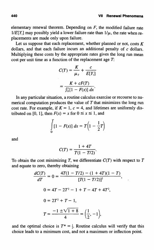
440 VII Renewal Phenomena
elementary renewal theorem. Depending on F, the modified failure rate1/E[Y,] may possibly yield a lower failure rate than 1/µ, the rate when re-placements are made only upon failure.
Let us suppose that each replacement, whether planned or not, costs Kdollars, and that each failure incurs an additional penalty of c dollars.Multiplying these costs by the appropriate rates gives the long run meancost per unit time as a function of the replacement age T:
_ K C
C(T) - + E[YE]lur
K + cF(T )
f o [ l - F(x)] dx .
In any particular situation, a routine calculus exercise or recourse to nu-merical computation produces the value of T that minimizes the long runcost rate. For example, if K = 1, c = 4, and lifetimes are uniformly dis-tributed on [0, 1], then F(x) = x for 0 :5 x : 1, and
f [F(x)] dx = T I 1- 2 T)0 \\
and
1 + 4TC(T) =
T(1 - T/2)
To obtain the cost minimizing T, we differentiate C(T) with respect to Tand equate to zero, thereby obtaining
dC(T) - - 4T(1 - T/2) - (1 + 4T)(1 - T)dT
- 0 - [T(1 - T/2)]2
0=4T-2T2- 1 +T-4T+4T2,
0=2T2+T- 1,
-1±V1_ _+8 1
T= 4
and the optimal choice is T* = 2. Routine calculus will verify that thischoice leads to a minimum cost, and not a maximum or inflection point.

4. The Asymptotic Behavior of Renewal Processes 441
4.2. The Renewal Theorem for Continuous Lifetimes
The elementary renewal theorem asserts that
limM(t) = 1-
!-x t /I.
It is tempting to conclude from this that M(t) behaves like t/µ as t growslarge, but the precise meaning of the phrase "behaves like" is rather sub-tle. For example, suppose that\all of the lifetimes are deterministic, sayX, = 1 for k = 1, 2, .... Then it is straightforward to calculate
M(t) = N(t) = 0 for 0 t < 1,
= 1 for I t < 2,
k 1.
That is, M(t) = [t], where [t] denotes the greatest integer not exceeding t.Since A = 1 in this example, then M(t) - t/µ = [t] - t, a function that os-cillates indefinitely between 0 and -1. While it remains true in this illus-tration that M(t)/t = [t]/t- 1 = l/µ, it is not clear in what sense M(t) "be-haves like" t/µ. If we rule out the periodic behavior that is exemplified inthe extreme by this deterministic example, then M(t) behaves like t/µ inthe sense described by the renewal theorem, which we now explain. LetM(t, t + h] = M(t + h) - M(t) denote the mean number of renewals inthe interval (t, t + h]. The renewal theorem asserts that when periodic be-havior is precluded, then
limM(t, t + h] = h/µ for any fixed h > 0. (4.2)
In words, asymptotically, the mean number of renewals in an interval isproportional to the interval's length, with proportionality constant 1/µ.
A simple and prevalent situation in which the renewal theorem (4.2) isvalid occurs when the lifetimes X X2, ... are continuous random vari-ables having the probability density function f(x). In this circumstance,the renewal function is differentiable, and
dM(t)m(t) = = 7 x (t), (4.3)
dt ,t_j
where f(t) is the probability density function for W = X, + + X,,.
Now (4.2) may be written in the form

442 VII Renewal Phenomena
M(t+h)-M(t) 1- - ast -->h
00,µ
which, when h is small, suggests that
lim m(t) = limdM(t) = 1
,mar ty- dt(4.4)
and indeed, this is the case in all but the most pathological of circum-stances when X1, X,, . . . are continuous random variables.
If in addition to being continuous, the lifetimes X, X,.... have a finitemean µ and finite variance 0.2, then the renewal theorem can be refined toinclude a second term. Under the stated conditions, we have
lim I M(t) - t Cr2 µ, (4.5)µ 2p-
Example When the lifetimes X,, X,, ... have the gamma densityfunction
f(x) = xe-' for x > 0, (4.6)
then the waiting times W,, = X, + + X have the gamma density
x(x) =f e-` for x > 0,
(2n - 1)!
as may be verified by performing the appropriate convolutions. (See I,Section 2.5.) Substitution into (4.3) yields
m(x) .f (x) _
and
M(t) = Jm(x)dx__t- 4 [1 - e--`].0
Since the gamma density in (4.6) has moments µ = 2 and 0.2 = 2, we

4. The Asymptotic Behavior of Renewal Processes 443
verify that m(t)-*1/µ as t--->oo and M(t) - tlµ--1 = (v.2 - µ2)12µ2, inagreement with (4.4) and (4.5).
4.3. The Asymptotic Distribution of N(t)
The elementary renewal theorem
E[N(t)] - 1lim-' - (4.7)t
A
implies that the asymptotic mean of N(t) is approximately t/µ. WhenE[Xj -and 0.2 = Var[XA ] = E[(Xk - µ)'-] are finite, then the asymp-
totic variance of N(t) behaves according to
limVar[N(t)]
=V,
(4.8)t-- tµ
.
That is, the asymptotic variance of N(t) is approximately to-'/µ3. If westandardize N(t) by subtracting its asymptotic mean and dividing by itsasymptotic standard deviation, we get the following convergence to thenormal distribution:
(N(t) - tlµ 1
lim Pr tW21µ3 x}
=2
X
J e dy.
In words, for large values of t the number of renewals N(t) is approxi-mately normally distributed with mean and variance given by (4.7) and(4.8), respectively.
4.4. The Limiting Distribution of Age and Excess Life
Again we assume that the lifetimes X,, X2, . . . are continuous randomvariables with finite mean µ. Let y, = WV,,,+, - t be the excess life at timet. The excess life has the limiting distribution
lim Pr{y, 5 x} = 1J
[1 - F(y)] dy. (4.9)r co

444 VII Renewal Phenomena
The reader should verify that the right side of (4.9) defines a valid distri-bution function, which we denote by H(x). The corresponding probabilitydensity function is h(y) = µ ' [ 1 - F(y)]. The mean of this limiting dis-tribution is determined according to
x 00
f yh(y) dy = 1 Jy[1 - F(y)] dyo µ'o
x x
= 1 JY{Jf(t) dt dy
µJ f(t) J y \dy dtv o
x
1 f t2f(t) dt2µ o
a.2+µ'-= 2µ '
where u2 is the common variance of the lifetimes X,, XZ.... .
{y,?xand6,?y} ifandonlyif {y,_y._x+y}. (4.10)
It follows that
limPr{y, a: x, 3,?y} = limPr{y,_,?x + y)
x
= µ-' J [1 - F(z)] dz,x+y
exhibiting the joint limiting distribution of (y S). In particular,
limPr{S, ? y} = limPr{y, ? 0, S, ? y}
x
= µ ' J [1 - F(z)] dzy
= 1 - H(y).

Exercises 445
The limiting distribution for the current life, or age, S, = t - W,(,) canbe deduced from the corresponding result (4.9) for the excess life. Withthe aid of Figure 4.1, corroborate the equivalence
N(t)
_X + y r-J
fE- Y -)FF- x _0
I 'Y,- t
Figure4.1 {5,>--sand y, ?x) if and only if {y,_,.>_x+y}.
Exercises
4.1. Consider the triangular lifetime density f(x) = 2x for 0 < x < 1.Determine an asymptotic expression for the expected number of renewalsup to time t.
Hint: Use equation (4.5).
4.2. Consider the triangular lifetime density f(x) = 2x for 0 < x < 1.Determine an asymptotic expression for the probability distribution of ex-cess life. Using this distribution, determine the limiting mean excess lifeand compare with the general result following equation (4.9).
4.3. Consider the triangular lifetime density function f(x) = 2x, for0 < x < 1. Determine the optimal replacement age in an age replacementmodel with replacement cost K = 1 and failure penalty c = 4 (cf. the ex-ample in Section 4.1).

446 VII Renewal Phenomena
4.4. Show that the optimal age replacement policy is to replace uponfailure alone when lifetimes are exponentially distributed with parameterA. Can you provide an intuitive explanation?
4.5. What is the limiting distribution of excess life when renewal life-times have the uniform density f(x) = 1, for 0 < x < 1?
4.6. A machine can be in either of two states: "up" or "down." It is upat time zero and thereafter alternates between being up and down. Thelengths X,, X,.... of successive up times are independent and identicallydistributed random variables with mean a, and the lengths Y,, Y,, ... ofsuccessive down times are independent and identically distributed withmean /3.
(a) In the long run, what fraction of time is the machine up?(b) If the machine earns income at a rate of $13 per unit time while up,
what is the long run total rate of income earned by the machine?(c) If each down time costs $7, regardless of how long the machine is
down, what is the long run total down time cost per unit time?
Problems
4.1. Suppose that a renewal function has the form M(t) = t +[1 - exp(-at)]. Determine the mean and variance of the interoccurrencedistribution.
4.2. A system is subject to failures. Each failure requires a repair timethat is exponentially distributed with rate parameter a. The operating timeof the system until the next failure is exponentially distributed with rateparameter /3. The repair times and the operating times are all statisticallyindependent. Suppose that the system is operating at time 0. Using equa-tion (4.5), determine an approximate expression for the mean number offailures up to time t, the approximation holding for t >> 0.
4.3. Suppose that the life of a light bulb is a random variable X withhazard rate h(x) = Ox for x > 0. Each failed light bulb is immediately re-placed with a new one. Determine an asymptotic expression for the meanage of the light bulb in service at time t, valid for t >> 0.

5. Generalizations and Variations on Renewal Processes 447
4.4. A developing country is attempting to control its population growthby placing restrictions on the number of children each family can have.This society places a high premium on female children, and it is felt thatany policy that ignores the desire to have female children will fail. Theproposed policy is to allow any married couple to have children up to thefirst female baby, at which point they must cease having children. Assumethat male and female children are equally likely. The number of childrenin any family is a random variable N. In the population as a whole, whatfraction of children are female? Use the elementary renewal theorem tojustify your answer.
4.5. A Markov chain X,,, X,, X,, ... has the transition probability matrix
0 1 2
0 0.3 0.7 0
P=1 0.6 0 0.4
2 0 0.5 0.5
A sojourn in a state is an uninterrupted sequence of consecutive visits tothat state.
(a) Determine the mean duration of a typical sojourn in state 0.(b) Using renewal theory, determine the long run fraction of time that
the process is in state 1.
5. Generalizations and Variationson Renewal Processes
5.1. Delayed Renewal Processes
W e continue to assume that {XR) are all independent positive random vari-ables, but only X,, X,, ... (from the second on) are identically distributedwith distribution function F, while X, has possibly a different distributionfunction G. Such a process is called a delayed renewal process. We haveall the ingredients for an ordinary renewal process except that the initialtime to the first renewal has a distribution different from that of the otherinteroccurrence times.

448 VII Renewal Phenomena
A delayed renewal process will arise when the component in operationat time t = 0 is not new, but all subsequent replacements are new. For ex-ample, suppose that the time origin is taken y time units after the start ofan ordinary renewal process. Then the time to the first renewal after theorigin in the delayed process will have the distribution of the excess lifeat time y of an ordinary renewal process.
As before, let Wo = 0 and W = X, + + X,,, and let N(t) count thenumber of renewals up to time t. But now it is essential to distinguish be-tween the mean number of renewals in the delayed process
MD(t) = E[N(t)], (5.1.)
and the renewal function associated with the distribution F,
M(t) Fk(t). (5.2)k=1
For the delayed process the elementary renewal theorem is
MD(t) = 1lim t -, where µ = E[XZ], (5.3)t-4= A
and the renewal theorem states that
hlim [MD(t) - MD(t - h)] = -,
provided XZ, X,, . . . are continuous random variables.
5.2. Stationary Renewal Processes
A delayed renewal process for which the first life has the distributionfunction
X
G(x) = IL' Ji - F(y) } dy0
is called a stationary renewal process. We are attempting to model a re-newal process that began indefinitely far in the past, so that the remaininglife of the item in service at the origin has the limiting distribution of theexcess life in an ordinary renewal process. We recognize G as this limit-ing distribution.

S. Generalizations and Variations on Ranewal Processes 449
It is anticipated that such a process exhibits a number of stationary, ortime-invariant, properties. For a stationary renewal process,
tMD(t) = E[N(t)] = - (5.4)
A
and
Pr{ y'D x) = G(x),
for all t. Thus, what is in general\,only an asymptotic renewal relation be-comes an identity, holding for a stationary renewal process.
5.3. Cumulative and Related Processes
Suppose associated with the ith unit, or lifetime interval, is a second ran-dom variable Y ({Y } identically distributed) in addition to the lifetime X;.We allow X; and Y to be dependent but assume that the pairs (X,, Y,),(X,, K,).... are independent. We use the notation F(x) = Pr{X; <_ x},G(y)=Pr{Y;sy},IL =E[X;], and v=E[Y].
A number of problems of practical and theoretical interest have a nat-ural formulation in those terms.
Renewal Processes Involving Two Components to EachRenewal Interval
Suppose that Y represents a portion of the duration X;. Figure 5.1 illus-trates the model. There we have depicted the Y portion occurring at the
-.*- YZ -
X, `14X2 X3H
Figure 5.1 A renewal process in which an associated random variable Y,_represents a portion of the ith renewal interval.

450 VII Renewal Phenomena
beginning of the interval, but this assumption is not essential for the re-sults that follow.
Let p(t) be the probability that t falls in a Y portion of some renewal in-terval. When X,, X,, ... are continuous random variables, the renewal the-orem implies the following important asymptotic evaluation:
limp(t) = E[Y](5.5)
E[X,]'
Here are some concrete examples.
A Replacement Model Consider a replacement model in which re-placement is not instantaneous. Let Y be the operating time and Z; the lagperiod preceding installment of the (i + 1)st operating unit. (The delayin replacement can be conceived as a period of repair of the service unit.)We assume that the sequence of times between successive replacementsX, = Y, + Z., k = 1, 2, . . . , constitutes a renewal process. Then p(t), theprobability that the system is in operation at time t, converges toE[Y,]/E[X,].
A Queueing Model A queueing process is a process in which cus-tomers arrive at some designated place where a service of some kind isbeing rendered, for example, at the teller's window in a bank or beside thecashier at a supermarket. It is assumed that the time between arrivals, orinterarrival time, and the time that is spent in providing service for a givencustomer are governed by probabilistic laws.
If arrivals to a queue follow a Poisson process of intensity A, then thesuccessive times X, from the commencement of the kth busy period to thestart of the next busy period form a renewal process. (A busy period is anuninterrupted duration when the queue is not empty.) Each X, is composedof a busy portion Z,, and an idle portion Y. Then p(t), the probability thatthe queue is empty at time t, converges to E[Y,]/E[X,]. This example istreated more fully in IX, which is devoted to queueing systems.
The Peter Principle The "Peter Principle" asserts that a worker willbe promoted until finally reaching a position in which he or she is incom-petent. When this happens, the person stays in that job until retirement.Consider the following single job model of the Peter Principle: A personis selected at random from the population and placed in the job. If the per-son is competent, he or she remains in the job for a random time having

5. Generalizations and Variations on Renewal Processes 451
cumulative distribution function F and mean µ and is promoted. Ifincompetent, the person remains for a random time having cumulativedistribution function G and mean v > µ and retires. Once the job is va-cated, another person is selected at random and the process repeats.Assume that the infinite population contains the fraction p of competentpeople and q = 1 - p incompetent ones.
In the long run, what fraction of time is the position held by an incom-petent person?
A renewal occurs every time that the position is filled, and therefore themean duration of a renewal cycle is
E[Xk] = pp. + (1 - p)v.
To answer the question, we let Yk = Xk if the kth person is incompetent,and Yk = 0 if the kth person is competent. Then the long run fraction oftime that the position is held by an incompetent person is
E[Y1] _ (1 - p)vE[X1] pµ + (1 - p)v'
Suppose that p = i of the people are competent, and that v = 10, whileµ = 1. Then
E[Y,] (1/2)(10) _ 10 _0 91
-E[X1] (1/2)(10) + (1/2)(1) 11
..-Thus, while half of the people in the population are competent, the job isfilled by a competent person only 9 percent of the time!
Cumulative Processes
Interpret Y; as a cost or value associated with the ith renewal cycle. A classof problems with a natural setting in this general context of pairs (X,, Y),where X, generates a renewal process, will now be considered. Interesthere focuses on the so-called cumulative process
N(t)+ I
W(t) _ 7. Yk,k=1
the accumulated costs or value up to time t (assuming that transactions aremade at the beginning of a renewal cycle).

452 V11 Renewal Phenomena
The elementary renewal theorem asserts in this case that
lim1
E[W(t)] = E[I] (5.6)1- - t
This equation justifies the interpretation of E[Y,]/µ as a long run meancost or value per unit time, an interpretation that was used repeatedly inthe examples of Section 2.
Here are some examples of cumulative processes.
Replacement Models Suppose Y; is the cost of the ith replacement. Letus suppose that under an age replacement strategy (see Section 3 and the ex-ample entitled "Age Replacement Policies" in Section 4) a planned re-placement at age T costs c, dollars, while a failure replaced at time x < Tcosts c2 dollars. If Yk is the cost incurred at the kth replacement cycle, then
Yk =1C2
with probability 1 - F(T),with probability F(T),
and E[Yk] = c,[l - F(T)] + c2F(T). Since the expected length of a re-placement cycle is
T
E[min{Xk, T}] = f [1 - F(x)] dx,0
we have that the long run cost per unit time is
c,[1 - F(T)] + c,F(T)fa[l -F(x)]dx
and in any particular situation a routine calculus exercise or recourse tonumerical computation produces the value of T that minimizes the longrun cost per unit time.
Under a block replacement policy, there is one planned replacementevery T units of time and, on the average, M(T) failure replacements, sothe expected cost is E[Yk] = c, + c,M(T), and the long run mean cost perunit time is {c, + CAT)}/T.
Risk Theory Suppose claims arrive at an insurance company accord-ing to a renewal process with interoccurrence times X,, X,..... Let Yk be

5. Generalizations and Variations on Renewal Processes 453
the magnitude of the kth claim. Then W(t) = k '; Y, represents the cu-mulative amount claimed up to time t, and the long run mean claim rate is
E[Yjlim t E[W(t)] =
E[X,]
Maintaining Current Control of a Process A production processproduces items one by one. At any instance, the process is in one of twopossible states, which we label iris control and out-of-control. These statesare not directly observable. Production begins with the process in-control,and it remains in-control for a random and unobservable length of timebefore a breakdown occurs, after which the process is out-of-control. Acontrol chart is to be used to help detect when the out-of-control state oc-curs, so that corrective action may be taken.
To be more specific, we assume that the quality of an individual item isa normally distributed random variable having an unknown mean and aknown variance a2. If the process is in-control, the mean equals a standardtarget, or design value, A, Process breakdown takes the form of shift inmean away from standard to µ, = I± Sv, where S is the amount of theshift in standard deviation units.
The Shewhart control chart method for maintaining process controlcalls for measuring the qualities of the items as they are produced and thenplotting these qualities versus time on a chart that has lines drawn at thetarget value A, and above and below this target value at A0 ± ko, where kis a parameter of the control scheme being used. As long as the plottedqualities fall inside these so-called action lines at p ± kcr, the process isassumed to be operating in-control, but if ever a point falls outside theselines, the process is assumed to have left the in-control state, and investi-gation and repair are instituted. There are obviously two possible types oferrors that can be made while thus controlling the process: (1) needless in-vestigation and repair when the process is in-control yet an observed qual-ity purely by chance falls outside the action lines and (2) continued oper-ation with the process out-of-control because the observed qualities arefalling inside the action lines, again by chance.
Our concern is the rational choice of the parameter k, that is, the ratio-nal spacing of the action lines, so as to balance, in some sense, these twopossible errors.

454 VII Renewal Phenomena
The probability that a single quality will fall outside the action lineswhen the process is in-control is given by an appropriate area under thenormal density curve. Denoting this probability by a, we have
a = (D(-k) + 1 - I(k) = 2c(-k),where 1(x) = (21r)-"2 fT, exp(-y2/2) dy is the standard cumulative nor-mal distribution function. Representative values are given in the follow-ing table:
k a
1.645 0.101.96 0.05
Similarly, the probability, denoted by p, that a single point will fall out-side the action lines when the process is out-of-control is given by
p=(D(-6-k)+ 1 -4)(-6+k).Let S denote the number of items inspected before an out-of-control signalarises assuming that the process is out-of-control. Then Pr{S = 1) = p,Pr(S = 2) = (1 - p)p, and in general, Pr(S = n) = (1 - p)"-'p. Thus, Shas a geometric distribution, and
E[S]p
Let The the number of items produced while the process is in-control. Wesuppose that the mean operating time in-control E[T] is known from pastrecords.
The sequence of durations between detected and repaired out-of-control conditions forms a renewal process because each such durationbegins with a newly repaired process and is a probabilistic replica of allother such intervals. It follows from the general elementary renewaltheorem that the long run fraction of time spent out-of-control (O.C.) is
E[S] _ 1
O.C. =E[S] + E[T] 1 + pE[T]
The long run number of repairs per unit time is
_ 1 _ pR
E[S] + E[T] 1 + pE[T]

Exercises 455
Let N be the random number of "false alarms" while the process is in-control, that is, during the time up to T, the first out-of-control. Then, con-ditioned on T, the random variable N has a binomial distribution withprobability parameter a, and thus E[NIT} = aT and E[N] = aE[T].Again, it follows from the general elementary renewal theorem that thelong run false alarms per unit time'(F.A.) is
E[N] apE[T]F.A. =
E[S] + E['] = 1 + pE[T]
If each false alarm costs c dollars, each repair cost K dollars, and thecost rate while operating out-of-control is C dollars, then we have the longrun average cost per unit time of
A.C. = C(O.C.) + K(R) + c(F.A.)
_ C + Kp + capE[T]1 + pE[T]
By trial and error one may now choose k, which determines a and p, soas to minimize this average cost expression.
Exercises
5.1. Jobs arrive at a certain service system according to a Poissonprocess of rate A. The server will accept an arriving customer only if it isidle at the time of arrival. Potential customers arriving when the system isbusy are lost. Suppose that the service times are independent random vari-ables with mean service time A. Show that the long run fraction of timethat the server is idle is 1/(1 + Aµ). What is the long run fraction of po-tential customers that are lost?
5.2. The weather in a certain locale consists of alternating wet and dryspells. Suppose that the number of days in each rainy spell is Poisson dis-tributed with parameter 2, and that a dry spell follows a geometric distri-bution with a mean of 7 days. Assume that the successive durations ofrainy and dry spells are statistically independent random variables. In thelong run, what is the probability on a given day that it will be raining?

456 VII Renewal Phenomena
5.3. Consider a light bulb whose life is a continuous random variable Xwith probability density function f(x), for x > 0. Assuming that one startswith a fresh bulb and that each failed bulb is immediately replaced by anew one, let M(t) = E[N(t)] be the expected number of renewals up totime t. Consider a block replacement policy (see Section 2.1) that replaceseach failed bulb immediately at a cost of c per bulb and replaces all bulbsat the fixed times T, 2T, 3T, .... Let the block replacement cost per bulbbe b < c. Show that the long run total mean cost per bulb per unit time is
O(T)= b+cM(T)T
Investigate the choice of a cost minimizing value T* when M(t) _t + 1 - exp(-at).
Problems
5.1. A certain type component has two states: 0 = OFF and 1 =OPERATING. In state 0, the process remains there a random length oftime, which is exponentially distributed with parameter a, and then movesto state 1. The time in state 1 is exponentially distributed with parameter/3, after which the process returns to state 0.
The system has two of these components, A and B, with distinctparameters:
Component Operating Failure Rate Repair Rate
A NA aA
B /3s ag
In order for the system to operate, at least one of components A and Bmust be operating (a parallel system). Assume that the component sto-chastic processes are independent of one another.
(a) In the long run, what fraction of time is the system inoperational(not operating)?
(b) Once the system enters the failed state, what is the mean durationthere prior to returning to operation?

6. Discrete Renewal Theory 457
(c) Define a cycle as the time between the instant that the system firstenters the failed state and the next such instant. Using renewal the-ory, find the mean duration of a cycle.
(d) What is the mean system operating duration between successivesystem failures?
5.2. The random lifetime X of an item has a distribution function F(x).What is the mean total life E[XI X >\x] of an item of age x?
5.3. At the beginning of each period, customers arrive at a taxi stand attimes of a renewal process with distribution law F(x). Assume an unlim-ited supply of cabs, such as might occur at an airport. Suppose that eachcustomer pays a random fee at the stand following the distribution lawG(x), for x > 0. Write an expression for the sum W(t) of money collectedat the stand by time t, and then determine the limit expectation
E[W(t)]limrax t
5.4. A lazy professor has a ceiling fixture in his office that contains twolight bulbs. To replace a bulb, the professor must fetch a ladder, and beinglazy, when a single bulb fails, he waits until the second bulb fails beforereplacing them both. Assume that the length of life of the bulbs are inde-pendent random variables.
(a) If the lifetimes of the bulbs are exponentially distributed, with thesame parameter, what fraction of time, in the long run, is our profes-sor's office half lit?
(b) What fraction of time, in the long run, is our professor's office halflit if the bulbs that he buys have the same uniform (0, 1) lifetimedistribution?
6. Discrete Renewal Theory*
In this section we outline the renewal theory that pertains to nonnegativeinteger-valued lifetimes. We emphasize renewal equations, the renewalargument, and the renewal theorem (Theorem 6.1).
* The discrete renewal model is a special case in the general renewal theory presentedin sections 1-5 and does not arise in later chapters.

458 VII Renewal Phenomena
Consider a light bulb whose life, measured in discrete units, is a ran-dom variable X where Pr{X = k} = pk for k = 0, 1, .... If one starts witha fresh bulb and if each bulb when it burns out is replaced by a new one,then M(n), the expected number of renewals (not including the initialbulb) up to time n, solves the equation
11
M(n) = FX(n) + pkM(n - k), (6.1)k=0
where FX(n) = p + + p,, is the cumulative distribution function of therandom variable X. A vector or functional equation of the form (6.1) in theunknowns M(0), M(1), ... is termed a renewal equation. The equation isestablished by a renewal argument, a first step analysis that proceeds byconditioning on the life of the first bulb and then invoking the law of totalprobability. In the case of (6.1), for example, if the first bulb fails at timek:5 n, then we have its failure plus, on the average, M(n - k) additionalfailures in the interval [k, k + 1, . . . , n]. We weight this conditional meanby the probability pk = Pr{X1 = k} and sum according to the law of totalprobability to obtain
M(n) _ [ 1 + M(n - k)]Pkk=0
F,(n)=LppM(n-k).k=0
Equation (6.1) is only a particular instance of what is called a renewalequation. In general, a renewal equation is prescribed by a given boundedsequence {bk } and takes the form
v =,1
for n = 0, 1, .... (6.2)k=0
The unknown variables are vo, v,, ... , and po, pi.... is a probability dis-tribution for which, to avoid trivialities, we always assume p < 1.
Let us first note that there is one and only one sequence vo, v,, . . . sat-isfying a renewal equation, because we may solve (6.2) successively toget

6. Discrete Renewal Weory 459
bovo = I - po ,
b, + p, vov,= I
- Po
for n = 0,for n > 0.
and so on.Let u,, be the mean number of renewals that take place exactly in period
n. When po = 0, so that the lifetime's are strictly positive and at most onerenewal can occur in any period, thei u,, is the probability that a single re-newal occurs in period n. The sequence u,,, u ... satisfies a renewal equa-tion that is of fundamental importance in the general theory. Let
Then {u } satisfies the renewal equation
k=0Pkun-k
(6.3)
(6.4)
for n = 0, 1, .... (6.5)
Again, equation (6.5) is established via a renewal argument. First, ob-serve that S counts the initial bulb, the renewal at time 0. Next, conditionon the lifetime of this first bulb. If it fails in period k < n, which occurswith probability pk, then the process begins afresh and the conditionalprobability of a renewal in period n becomes Weighting the contin-gency represented by by its respective probability pk and summing ac-cording to the law of total probability then yields (6.5).
The next lemma shows how the solution {v,,} to the general renewalequation (6.2) can be expressed in terms of the solution to the partic-ular equation (6.5).
Lemma 6.1 If { v } satisfies (6.2) and { u } satisfies (6.5), then
forn=0, 1,....k=0
Proof In view of our remarks on the existence and uniqueness of solu-tions to equation (6.2), we need only verify that v,, = Yk=o b-kuk satisfies(6.2). We have

460 VII Renewal Phenomena
v _k=0
=b
=b
= b
=b
=b
if
k=0 1=0
1=0 k=!
1=o j=o
j=0 1=0
j=0
b kPk-rui
pj ur
Example Let X, X,.... be the successive lifetimes of the bulbs and letWo = 0 and W = X, + + X,, be the replacement times. We assumethat p0, = Pr{X1 = 0) = 0. The number of replacements (not including theinitial bulb) up to time n is given by
N(n) = k for Wk <- n < Wk,,.
The M(n) = E[N(n)] satisfies the renewal equation (6.1)n
M(n) = po + ... + p + Z. PkM(n - k),k=0
and elementary algebra shows that m,, = E[N(n) + I] = M(n) + 1 satisfiesit
M" = 1 + for n = 0, 1, .... (6.6)k=0
Then (6.6) is a renewal equation for which b,, = I for all n. In view ofLemma 6.1 we conclude that

6. Discrete Renewal Theory 461
77
Mn = > . lug = up + + u,,.k=0
Conversely, u,, = m,, - m,,_, = M(n) - M(n - 1).To continue with the example, let g,, = E[WN(,,,+,] The definition is il-
lustrated in Figure 6.1. We will argue that g,, satisfies a certain renewalequation. As shown in Figure 6.1, always includes the first renewalduration X,. In addition, if X, = k : n, which occurs with probability pk,then the conditional mean of the added lives constituting WN(,,)+, isWeighting these conditional means by, their respective probabilities andsumming according to the law of total 'probability then gives
Hence, by Lemma 6.1,
g = E[XI] +k=0
pk.
g,, E[X,luk=E[X,lmk=0
We get the interesting formula [see (1.7)]
E[X, + + X E[N(n) + 1]. (6.7)
Note that N(n) is not independent of {Xk}, and yet (6.7) still prevails.
N(n)
X,
X,
Wo
X;
W, n
,
n
Figure 6.1 WN(,,)+I always contains X, and contains additional durations whenX, =k<--n.

462 VII Renewal Phenomena
6.1. The Discrete Renewal Theorem
The renewal theorem provides conditions under which the solution { v } toa renewal equation will converge as n grows large. Certain periodic be-havior, such as failures occurring only at even ages, must be precluded,and the simplest assumption assuring this preclusion is that p, > 0.
Theorem 6.1 Suppose that 0 < p, < 1 and that and are the. solutions to the renewal equations (6.5) and (6.2), respectively. Then(a) u,, = 1/j okpk; and (b) if <00, then{Y,A obk}/{T1A okPk}.
We recognize that Yk=okp, = E[X,] is the mean lifetime of a unit. Thus(a) in Theorem 6.1 asserts that in the long run, the probability of a renewaloccurring in a given interval is one divided by the mean life of a unit.
Remark Theorem 6.1 holds in certain circumstances when p, = 0. Itsuffices to assume that the greatest common divisor of the integers k forwhich pk > 0 is one.
Example Let y,, = WN,,,,+, - n be the excess life at time n. For a fixedinteger m, let f(m) = Pr{y = m}. We will establish a renewal equationfor f(m) by conditioning on the first life X. For m > 1,
if 0:5 k <- n,1 ifk=n+m,
10 otherwise.
(The student is urged to diagram the alternatives arising inPr{y = mIX, = k}.) Then, by the law of total probability,
=7' =k}pkk=o
it (6.8)
P,,,+ + L f -k(m)Pkk=O
We apply Theorem 6.1 with b,, = p,, + to conclude that

6. Discrete Renewal Theory 463
lim Pr{y = m} _"k=0 Pw+k
7-i=o kPk
Pr{X,? m}
E[X,] 'm= 1,2,....
The limit is a bona fide probability mass function, since its terms sumto one:
Pr{X1 ? m} _ E[X,] = 1.E[XI] E[XI]
6.2. Deterministic Population Growth with Age Distribution
In this section we will discuss a simple deterministic model of populationgrowth that takes into account the age structure of the population. Sur-prisingly, the discrete renewal theorem (Theorem 6.1) will play a role inthe analysis. As the language will suggest, the deterministic model that wetreat may be viewed as describing the mean population size in a moreelaborate stochastic model that is beyond our scope to develop fully.
A Simple Growth Model Let us set the stage by reviewing a simplemodel that has no age structure. We consider a single species evolving indiscrete time t = 0, 1, 2, ... , and we let N, be the population size at timet. We assume that each individual present in the population at time t givesrise to a constant number A of offspring that form the population at timet + 1. (If death does not occur in the model, then we include the parent asone of the offspring, and then necessarily A ? 1.) If No is the initial popu-lation size, and each individual gives rise to X offspring, then
N,=AN,
N,=AN,=A'NQ,
and in general,
N, = A'N0. (6.9)

464 VII Renewal Phenomena
If A > 1, then the population grows indefinitely in time; if A < 1, then thepopulation dies out; while if A = 1, then the population size remains con-stant at N, = No for all t = 0, 1, ... .
The Model with Age Structure We shall now introduce an agestructure in the population. We need the following notation:
n,,,, = the number of individuals of age u in the population at time t;
N, = Y,;;=o n,,., = the total number of individuals in the population attime t;
b, = the number of new individuals created in the population at timet, the number of births;
/3 = the expected number of progeny of a single individual of age uin one time period;
l = the probability that an individual will survive, from birth, atleast to age u.
The conditional probability that an individual survives at least to age u,given that is has survived to age u - 1, is simply the ration The netmaternity function is the product
M.
and is the birth rate adjusted for the death of some fraction of the popula-tion. That is, m is the expected number of offspring at age u of an indi-vidual now of age 0.
Let us derive the total progeny of a single individual during its lifespan.An individual survives at least to age u with probability 1,,, and then dur-ing the next unit of time gives rise to /3 offspring. Summing mover all ages u then gives the total progeny of a single individual:
1"A' = . m,,. (6.10)u=0 N=0
If M > 1, then we would expect the population to increase over time; ifM < 1, then we would expect the population to decrease; while if M = 1,then the population size should neither increase nor decrease in the longrun. This is indeed the case, but the exact description of the populationevolution is more complex, as we will now determine.

6. Discrete Renewal Theory 465
In considering the effect of age structure on a growing population, ourinterest will center on b,, the number of new individuals created in thepopulation at time t. We regard 6,,, 1,,, and n,,.0 as known, and the problemis to determine b, for t ? 0. Once b, is known, then n,,., and N, may be de-termined according to, for example,
no., = bl,
1nu.l = nu-I,0
lu-1
(6.11)
for u 1, (6.12)
and
N, =u=0
uJ* (6.13)
In the first of these simple relations, no.,, is the number in the populationat time 1 of age 0, which obviously is the same as b those born in thepopulation at time 1. For the second equation, n,,., is the number in thepopulation at time 1 of age u. These individuals must have survived fromthe individuals in the population at time 0 of age u - 1; the condi-tional probability of survivorship is which explains the secondequation. The last relation simply asserts that the total population size re-sults by summing the numbers of individuals of all ages. The generaliza-tions of (6.11) through (6.13) are
no., = b,, (6.14)
n,,,, = for u ? 1, (6.15)
and
x
N, _ n,,,, fort ? 1.1,=0
(6.16)
Having explained how n,,,, and N, are found once b, is known, we turnto determining b,. The number of individuals created at time t has twocomponents. One component, a,, say, counts the offspring of those indi-viduals in the population at time t who already existed at time 0. In thesimplest case, the population begins at time t = 0 with a single ancestorof age u = 0, and then the number of offspring of this individual at time tis a, = m,, the net maternity function. More generally, assume that there

466 VII Renewal Phenomena
were n,,.o individuals of age u at time 0. The probability that an individualof age u at time 0 will survive to time t (at which time it will be of aget + u) is Hence the number of individuals of age u at time 0 thatsurvive to time t is and each of these individuals, now of aget + u, will produce (3,+ new offspring. Adding over all ages we obtain
1,+
_ m,+,,n,,.o
11=0 1
L P,+,,n,,.o-1
(6.17)
The second component of b, counts those individuals created at time twhose parents were not initially in the population but were born after time0. Now, the number of individuals created at time T is b_. The probabilitythat one of these individuals survives to time t, at which time he will beof age t - T, is 1,-,. The rate of births for individuals of age t - 'r isThe second component results from summing over r and gives
b, = a, +>. 01-711-:br
= a,
r=O
(6.18)
Example Consider an organism that produces two offspring at age 1,and two more at age 2, and then dies. The population begins with a singleorganism of age 0 at time 0. We have the data
no.o = 1, n,,.o = 0 for u ? 1,
b,=b,=2,10=1,=1,=1 and 1,,=0 foru>2.
We calculate from (6.17) that
a,=O, a, = 2, a,=2, and a, = 0, for t > 2.
Finally, (6.18) is solved recursively as
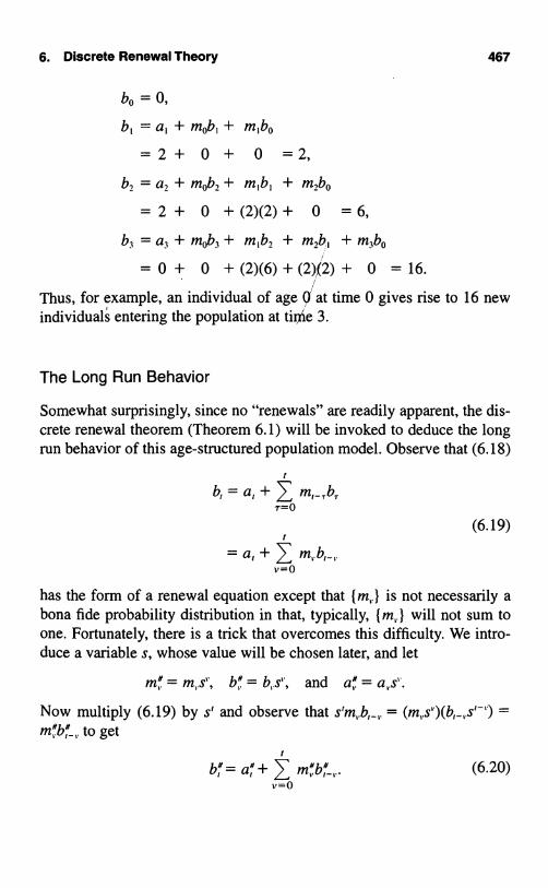
6. Discrete Renewal Theory 467
bo = 0,
b, = a, + mob, + m,bo
=2+ 0 + 0 =2,
b, = a, + mob, + m,b, + m,bo
= 2 + 0 + (2)(2) + 0 = 6,
b3 = a, + mob, + m,b, + m,b, + m,bo
= 0 + 0 + (2)(6) + (2)(2) + 0 = 16.
Thus, for example, an individual of age 0(at time 0 gives rise to 16 newindividuals entering the population at time 3.
The Long Run Behavior
Somewhat surprisingly, since no "renewals" are readily apparent, the dis-crete renewal theorem (Theorem 6.1) will be invoked to deduce the longrun behavior of this age-structured population model. Observe that (6.18)
(6.19)
a,
has the form of a renewal equation except that {m,.} is not necessarily abona fide probability distribution in that, typically, {m,.} will not sum toone. Fortunately, there is a trick that overcomes this difficulty. We intro-duce a variable s, whose value will be chosen later, and let
m,,,, = m,.s', b,," = b,.s and a" = a,.s'.
Now multiply (6.19) by s' and observe that s'm,.b,-,, = (m,.s'')(b,_,,s'-'')m"br"_, to get
b # = a" + > m,",b,"_,.. (6.20)

468 VII Renewal Phenomena
This renewal equation holds no matter what value we choose for s. Wetherefore choose s such that (m,". } is a bona fide probability distribution.That is, we fix the value of s such that
xMI.
vO
There is always a unique such s whenever 1 < J;,=o m, < oo. We may nowapply the renewal theorem to (6.20), provided that its hypothesis con-cerning nonperiodic behavior is satisfied. For this it suffices, for example,that m, > 0. Then we conclude that
x y
lim b," = lim bs' = ".!fix !fix 2.,.=o vm,.
(6.21)
We set A = 1/s and K = x=o a,"/E=o vm," to write (6.21) in the form
b, - KA' for t large.
In words, asymptotically, the population grows at rate A where A = 1/s isthe solution to
tc
,.A-" = 1.=0
When t is large (t > u), then (6.15) may be iterated in the manner
ln,,.,
r l
l= no.,
1101 =
This simply expresses that those of age u at time t were born t - u timeunits ago and survived. Since for large t we have b,- =- KA'-", then

Exercises 469
n,,., K(l,k-u)n',
N, = >, nu., K.. (l,, lc )A',
and
lim n,,., _ l"A-U
- N, Y,xV-v*
This last expression furnishes the asymptotic, or stable, age distributionin the population.
Example Continuing the example in which m, = m2 = 2 and mk = 0otherwise, then we have
xI m,,s"=2s+2s22= 1,v=o
which we solve to obtain
-2±V4 + 8 -1 ±vs= 4 = 2
_ (0.366, -1.366).
The relevant root is s = 0.366, whence A = 1/s = 2.732. Thus asymptot-ically, the population grows geometrically at rate A = 2.732 , and thestable age distribution is as shown in the following table:
Age Fraction of Population
0 1/(1 + s + s2) = 0.66671 s/(1 + s + s2) = 0.24402 s2/(1 + s + s2) = 0.0893
Exercises
6.1. Solve for v,, for n = 0, 1, ... , 10 in the renewal equation
PkV,,-k forn=0, 1,...,k=0
where b0=b, =2, b2=b3=... =0,andpo=4, p, =i, and P2=4.

470 VII Renewal Phenomena
6.2. (Continuation of Exercise 6.1)
(a) Solve for u,, for n = 0, 1, ... , 10 in the renewal equation
u = S)!
k=0forn=0,1,...,
where So = 1, S, = S, _ = 0, and {pk} is as defined in Exercise6.1.
(b) Verify that the solution v,, in Exercise 6.1 and u,, are related accord-ing to v,, =
6.3. Using the data of Exercises 6.1 and 6.2, determine
(a) u,,.
(b) lim,,, v,,.
Problems
6.1. Suppose the lifetimes X, X2, ... have the geometric distribution
Pr{X1 = k} = a(l - a)k-' fork = 1, 2, ... ,where 0<a<1.
(a) Determine u,, for n = 1, 2, ... .(b) Determine the distribution of excess life y by using Lemma 6.1
and (6.8).
6.2. Marlene has a fair die with the usual six sides. She throws the dieand records the number. She throws the die again and adds the secondnumber to the first. She repeats this until the cumulative sum of all thetosses first exceeds a prescribed number n. (a) When n = 10, what is theprobability that she stops at a cumulative sum of 13? (b) When n is large,what is the approximate probability that she stops at a sum of n + 3?
6.3. Determine the long run population growth rate for a populationwhose individual net maternity function is m, = m; = 2, and mk = 0otherwise. Why does delaying the age at which offspring are first pro-duced cause a reduction in the population growth rate? (The population

Problems 471
growth rate when m, = m, = 2, and mk = 0 otherwise was determined inthe last example of this section.)
6.4. Determine the long run population growth rate for a populationwhose individual net maternity function is mo = m, = 0 and m2 =m, = = a > 0. Compare this with the population growth rate whenm,= a, andm,=0fork 2.


Chapter VIIIBrownian Motion and
Related Processes
1. Brownian Motion and Gaussian Processes
The Brownian motion stochastic process arose early in this century as anattempt to explain the ceaseless irregular motions of tiny particles sus-pended in a fluid, such as dust motes floating in air. Today, the Brownianmotion process and its many generalizations and extensions occur in nu-merous and diverse areas of pure and applied science such as economics,communication theory, biology, management science, and mathematicalstatistics.
1.1. A Little History
The story begins in the summer of 1827, when the English botanist RobertBrown observed that microscopic pollen grains suspended in a drop ofwater moved constantly in haphazard zigzag trajectories. Following thereporting of his findings, other scientists verified the strange phenomenon.Similar Brownian motion was apparent whenever very small particleswere suspended in a fluid medium, for example, smoke particles in air.Over time, it was established that finer particles move more rapidly, thatthe motion is stimulated by heat, and that the movement becomes moreactive with a decrease in fluid viscosity.

474 VIII Brownian Motion and Related Processes
A satisfactory explanation had to wait until the next century, when in1905, Einstein would assert that the Brownian motion originates in thecontinual bombardment of the pollen grains by the molecules of the sur-rounding water, with successive molecular impacts coming from differentdirections and contributing different impulses to the particles. Einstein ar-gued that as a result of the continual collisions, the particles themselveshad the same average kinetic energy as the molecules. Belief in moleculesand atoms was far from universal in 1905, and the success of Einstein'sexplanation of the well-documented existence of Brownian motion didmuch to convince a number of distinguished scientists that such things asatoms actually exist. Incidentally, 1905 is the same year in which Einsteinset forth his theory of relativity and his quantum explanation for the pho-toelectric effect. Any single one of his 1905 contributions would havebrought him recognition by his fellow physicists. Today, a search in a uni-versity library under the subject heading "Brownian motion" is likely toturn up dozens of books on the stochastic process called Brownian motionand few, if any, on the irregular movements observed by Robert Brown.The literature on the model has far surpassed and overwhelmed the liter-ature on the phenomenon itself!
Brownian motion is complicated because the molecular bombardmentof the pollen grain is itself a complicated process, so it is not surprising thatit took more than another decade to get a clear picture of the Brownian mo-tion stochastic process. It was not until 1923 that Norbert Wiener set forththe modem mathematical foundation. The reader may also encounter"Wiener process" or "Wiener-Einstein process" as names for the stochas-tic process that we will henceforth simply call "Brownian motion."
Predating Einstein by several years, in 1900 in Paris, Louis Bachelierproposed what we would now call a "Brownian motion model" for themovement of prices in the French bond market. While Bachelier's paperwas largely ignored by academics for many decades, his work now standsas the innovative first step in a mathematical theory of stock markets thathas greatly altered the financial world of today. Later in this chapter, we willhave much to say about Brownian motion and related models in finance.
1.2. The Brownian Motion Stochastic Process
In terms of our general framework of stochastic processes (cf. I, Section1.1), the Brownian motion process is an example of a continuous-time,

1. Brownian Motion and Gaussian Processes 475
continuous-state-space Markov process. Let B(t) be the y component (as afunction of time) of a particle in Brownian motion. Let x be the positionof the particle at time to; i.e., x. Let p(y, t1x) be the probability den-sity function, in y, of B(to + t), given that x. We postulate that theprobability law governing the transitions is stationary in time, and there-fore p(y, tlx) does not depend on the initial time to.
Since p(y, t1 x) is a probability density function in y, we have theproperties
x
p(y, t1x) ? 0 andJ
p(y, t1x) dy = 1. (1.1)
Further, we stipulate that B(to ± t) is likely to be near B(to) = x for smallvalues of t. This is done formally by requiring that
limp(y, t1 x) = 0 for y * x. (1.2)r )0
From physical principles, Einstein showed that p(y, t1x) must satisfy thepartial differential equation
ap__ 0,,a2pat ax'-'
(1.3)
This is called the diffusion equation, and 0-22 is the diffusion coefficient,which Einstein showed to be given by Q'- = RTINf, where R is the gas con-stant, T is the temperature, N is Avogadro's number, and f is a coefficientof friction. By choosing the proper scale, we may take o-' = 1. With thischoice we can verify directly (See Exercise 1.3) that
p(Y> tax) = expl2t -x)21 (1.4)
is a solution of (1.3). In fact, it is the only solution under the conditions(1.1) and (1.2). We recognize (1.4) as a normal probability density func-tion whose mean is x and whose variance is t. That is, the position of theparticle t time units after observations begin is normally distributed. Themean position is the initial location x, and the variance is the time of ob-servation t.
Because the normal distribution will appear over and over in this chap-ter, we are amply justified in standardizing some notation to deal with it.

476 VIII Brownian Motion and Related Processes
Let
be the standard normal probability density function, and let
41(z) = J O(x) dx (1.6)-x
be the corresponding cumulative distribution function. A small table of thecumulative normal distribution appears at the end of this section (seep. 486). Let
1
¢(z/N/t-), (1.7)_Vrt
and
Z
INz) = f ¢,(x) dx = (D(zl V)-x
(1.8)
be the probability density function and cumulative distribution function,respectively, for the normal distribution with mean zero and variance t. Inthis notation, the transition density in (1.4) is given by
P(y, tlx) = 4,(y - x), (1.9)
and
XPr{B(t) <_ yIB(O) = x} _ y
The transition probability density function in (1.4) or (1.9) gives only theprobability distribution of B(t) - B(O). The complete description of theBrownian motion process with diffusion coefficient QZ is given by the fol-lowing definition.
Definition Brownian motion with diffusion coefficient v2 is a stochas-tic process {B(t); t ? 0} with the properties:
(a) Every increment B(s + t) - B(s) is normally distributed with meanzero and variance o 2t; o > 0 is a fixed parameter.

1. Brownian Motion and Gaussian Processes 477
(b) For every pair of disjoint time intervals (t t2], (t3i t,], with0 : t, < t2 C t3 < t,, the increments B(t,) - B(t3) and B(t) - B(t,)are independent random variables, and similarly for n disjoint timeintervals, where n is an arbitrary positive integer.
(c) B(0) = 0, and B(t) is continuous as a function of t.
The definition says that a displacement B(s + t) - B(s) is independentof the past, or alternatively, if we know B(s) = x, then no further knowl-edge of the values of B(T) for past times T < s has any effect onour knowledge of the probability law governing the future movementB(s + t) - B(s). This is a statement of the Markov character of theprocess. We emphasize, however, that the independent increment as-sumption (b) is actually more restrictive than the Markov property. A typ-ical Brownian motion path is illustrated in Figure 1.1.
B(t)
Figure 1.1 A typical Brownian motion path.

478 Vlll Brownian Motion and Related Processes
The choice B(O) = 0 is arbitrary, and we often consider Brownian mo-tion starting at x, for which B(O) = x for some fixed point x. For Brown-ian motion starting at x, the variance of B(t) is oat, and 0-2 is termed thevariance parameter in the stochastic process literature. The process b(t)= B(t)lo- is a Brownian motion process whose variance parameter is one,the so-called standard Brownian motion. By this device, we may alwaysreduce an arbitrary Brownian motion to a standard Brownian motion; forthe most part, we derive results only for the latter. By part (a) of the defi-nition, for a standard Brownian motion (v2 = 1), we have
Pr{B(s + t) : yIB(s) = x} = Pr(B(s + t) - B(s) : y - x}
yx
Remark Let us look, for the moment, at a Brownian displacementB(it) after a small elapsed time it. The mean displacement is zero, andthe variance of the displacement is it itself. It is much more common inpractical work to use a standard deviation, the square root of the variance,to measure variability. For the normal distribution, for instance, the prob-ability of an observation more than 2 standard deviations away from themean is about 5%, and the standard deviation is in the same units as theoriginal measurement, and not (units)'-. The standard deviation of theBrownian displacement is Vlt, which is much larger than it itselfwhen it is small. Indeed, StdDev[B(it)]/it = V/it = 1/V - oo asit - 0. This is simply another manifestation of the erratic movements ofthe Brownian particle, yet it is a point that Bachelier and others had diffi-culty in handling. But the variance, being linear in time, and not thestandard deviation, is the only possibility if displacements over disjointtime intervals are to be stationary and independent. Write a total dis-placement B(s + t) - B(0) as the sum of two incremental steps in the formB(s + t) - B(0) = {B(s) - B(0) } + {B(s + t) - B(s)). The incrementalsteps being statistically independent, their variances must add. The sta-tionary assumption is that the statistics of the second step B(t + s) - B(t)do not depend on the time t when the step began, but only on the durations of the movement. We must have, then, Var[B(t + s)] = Var[B(t)] +Var[B(s)], and the only nonnegative solution to such an equation is to havethe variance of the displacement a linear function of time.
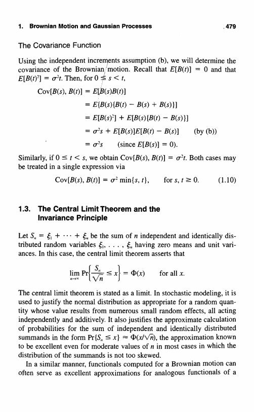
1. Brownian Motion and.Gaussian Processes .479
The Covariance Function
Using the independent increments assumption (b), we will determine thecovariance of the Brownian/motion. Recall that E[B(t)] = 0 and thatE[B(t)2] = 0-2 t. Then, for 0 s < t,
Cov[B(s), B(t)] = E[P(s)B(t)]
= E{B(s) {B(t) - B(s) + B(s) }]
= E[B(s)2] + E[B(s)(B(t) - B(s)}]
= 0-2 s + E[B(s)]E[B(t) - B(s)] (by (b))
= u2s (since E[B(s)] = 0).
Similarly, if 0 <_ t < s, we obtain Cov[B(s), B(t)] = 0-'t. Both cases maybe treated in a single expression via
Cov[B(s), B(t)] = Q.2 min{s, t}, for s, t ? 0. (1.10)
1.3. The Central Limit Theorem and theInvariance Principle
Let S,, _ , + + 6 be the sum of n independent and identically dis-tributed random variables 6 ... , having zero means and unit vari-ances. In this case, the central limit theorem asserts that
lim Prj x} _ fi(x) for all x.11-- n
The central limit theorem is stated as a limit. In stochastic modeling, it isused to justify the normal distribution as appropriate for a random quan-tity whose value results from numerous small random effects, all actingindependently and additively. It also justifies the approximate calculationof probabilities for the sum of independent and identically distributedsummands in the form Pr{S : x} c(x/V), the approximation knownto be excellent even for moderate values of n in most cases in which thedistribution of the summands is not too skewed.
In a similar manner, functionals computed for a Brownian motion canoften serve as excellent approximations for analogous functionals of a

480 All Brownian Motion and Related Processes
partial sum process, as we now explain. As a function of the continuousvariable t, define
, t ? 0,B,,(t) = SVn_
where [x] is the greatest integer less than or equal to x. Observe that
Sk V Sk k k 1
N/k'forn:5 t<n+n.
Because SklNIrk has unit variance, the variance of B (t) is [nt]ln, whichconverges to t as n - co. When n is large, then k = [nt] is large, and Sk/v-kis approximately normally distributed by the central limit theorem, and, fi-nally, B (t) inherits the independent increments property (b) from the pos-tulated independence of the summands. It is reasonable, then, to believethat B (t) should behave much like a standard Brownian motion process,at least when n is large. This is indeed true, and while we cannot explainthe precise way in which it holds in an introductory text such as this, thereader should leave with some intuitive feeling for the usefulness of theresult and, we hope, a motivation to learn more about stochasticprocesses. The convergence of the sequence of stochastic processes de-fined in (1.11) to a standard Brownian motion is termed the invarianceprinciple. It asserts that some functionals of a partial sum process of in-dependent and identically distributed zero mean and unit variance randomvariables should not depend too heavily on (should be invariant of) the ac-tual distribution of the summands, but be approximately given by theanalogous functional of a standard Brownian motion, provided only thatthe summands are not too badly behaved.
Example Suppose that the summands have the distribution in which1, each with probability Then the partial sum process S,, is a sim-
ple random walk for which we calculated in III, Section 5.3 (using a dif-ferent notation)
Pr{S reaches -a < 0 before b > O1So = 0}
_ b
a + b (1.12)

1. Brownian Motion and Gaussian Processes 481
Upon changing the scale in accordance with (1.11), we have
reaches -a < 0 before b > OISO = 0)
_ bV_n
=b
a+b'and invoking the invariance principle, it should be, and is, the case that fora standard Brownian motion we have
Pr{B(t) reaches -a < 0 before b > 01B(0) = 0)
_ b
a+b' (1.13)
Finally, invoking the invariance principle for a second time, the evaluationin (1.12) should hold approximately for an arbitrary partial sum process,provided only that the independent and identically distributed summandshave zero means and unit variances.
1.4. Gaussian Processes
A random vector X ... , X is said to have a multivariate normal dis-tribution, or a joint normal distribution, if every linear combinationa,X, + + a univariate normal distribution. Obvi-ously, if X ... , X,, has a joint normal distribution, then so does the ran-dom vector Y . . . , Ym, defined by the linear transformation in which
Y=a1,X,+ +a;,,X,,, forj= 1,...,m,for arbitrary constants a;;.
The multivariate normal distribution is specified by two parameters, themean values µ; = E[X;] and the covariance matrix whose entries areI;; = Cov[X;, X,]. In the joint normal distribution, I;; = 0 is sufficient toimply that X; and X, are independent random variables.
Let T be an abstract set and {X(t); t in T J a stochastic process. We call{X(t); tin T} a Gaussian process if for every n = 1, 2, ... and every fi-nite subset {t,, . . . , of T, the random vector (X(t,), . . . , X(t,,)) has amultivariate normal distribution. Equivalently, the process is Gaussian ifevery linear combination
a,X(t,) + + a; real,

482 VIII Brownian Motion and Related Processes
has a univariate normal distribution. Every Gaussian process is describeduniquely by its two parameters, the mean and covariance functions, givenrespectively by
µ(t) = E[X(t)], tin T,
and
r(s, t) = E[(X(s) - µ(s) } (X(t) - µ(t) }], s, tin T.
The covariance function is positive definite in the sense that for everyn = 1, 2, . . . , real numbers a...... a,,, and elements t...... t,, in T,
7, a,a;r(t,, t) ? 0.i=lj=l
One need only evaluate the expected value of a;(X(t) - µ(t;)})'- >_ 0in terms of the covariance function in order to verify this.
Conversely, given an arbitrary mean value function µ(t) and a positivedefinite covariance function F(s, t), there then exists a correspondingGaussian process. Brownian motion is the unique Gaussian process hav-ing continuous trajectories, zero mean, and covariance function (1.10).We shall use this feature, that the mean value and covariance functions de-fine a Gaussian process, several times in what follows.
We have seen how the invariance principle leads to the Gaussianprocess called Brownian motion. Gaussian processes also arise as the lim-its of normalized sums of independent and identically distributed randomfunctions. To sketch out this idea, let 1(t), 62(t), ... be independent andidentically distributed random functions, or stochastic processes. Letµ(t) = E[e(t)] and r(s, t) = fi(t)] be the mean value and co-variance functions, respectively. Motivated by the central limit theorem,we define
XN(t) _ 1=1 ( r^(t)- p(t)INN
The central limit theorem tells us that the distribution of X,,,(t) convergesto the normal distribution for each fixed time point t. A multivariate ex-tension of the central limit theorem asserts that for any finite set of timepoints (tl, ... , t,,), the random vector
(X, (tl), ... , XN(t,))

1. Brownian Motion and Gaussian Processes 483
has, in the limit for large N, a multivariate normal distribution. It is notdifficult to believe, then, that under ordinary circumstances, the stochasticprocesses {XN(t); t ? 0} would converge, in an appropriate sense, to aGaussian process {X(t); t ? 0) whose mean is zero and whose covariancefunction is F(s, t). We call this the central limit principle for random func-tions. Several instances of its application appear in this chapter, the first ofwhich is next.
Example Cable Strength Under Equal Load Sharing Consider acable constructed from N wires in parallel. Suspension bridge cables areusually built this way. A section of the cable is clamped at each end andelongated by increasing the distance between the clamps. The problem isto determine the maximum tensile load that the cable will sustain in termsof the probabilistic and mechanical characteristics of the individual wires.
Let Lo be the reference length of an unstretched unloaded strand of wire,and let L be the length after elongation. The nominal strain is defined tobe t = (L - Lo)/Lo. Steadily increasing t causes the strand to stretch andexert a force fi(t) on the clamps, up to some random failure strain , atwhich point the wire breaks. Hooke's law of elasticity asserts that the wireforce is proportional to wire strain, with Young's modulus K as the pro-portionality constant. Taken all together, we write the force on the wire asa function of the nominal strain as
Kt, for 0 - t<0 for t.
(1.14)
A typical load function is depicted in Figure 1.2 on the next page.We will let F(x) = Pr{C <_ x) be the cumulative distribution function of
the failure strain. We easily determine the mean load on the wire to be
µ(t) = E[a(t)] = E[Kt1{t < }] = Kt[1 - F(t)]. (1.15)
The higher moments are, for 0 < s < t,
K2stE[1{s < }1{t < fl]
= K2st[1 - F(t)]
and
F(s, t) = E[6(s)e(t)] -
K2stF(s)[1 - F(t)], for 0 < s < t. (1.16)

484 VIII Brownian Motion and Related Processes
Load
t (t)
t Strain t
Figure 1.2 The load on an elastic wire as a function of nominal strain. At astrain of the wire fails, and the load carried drops to zero.
Turning to the cable, if it is clamped at the ends and elongated, then eachwire within it is elongated the same amount. The total force SN(t) on thecable is the sum of the forces exerted by the individual wires. If we as-sume that the wires are independent and a priori identical, then these wireforces 6,(t), ,(t), ... are independent and identically distributed randomfunctions, and
SN(t) = i(t)i=1
is the random load experienced by the cable as a function of the cablestrain. An illustration when N = 5 is given in Figure 1.3.
We are interested in the maximum load that the cable could carry with-out failing. This is
QN = max{SN(t); t ? 0).

1. Brownian Motion and Gaussian Processes 485
Maximum sustainablecable load
I
Cable Strain t
Figure 1.3 The load experienced by a cable composed of five elastic wirestrands as a function of the cable strain t.
To obtain an approximation to the distribution of QN we apply the centrallimit principle for random functions. This leads us to believe that
XN(t) =SN(t)
VNY
should, for large N, be approximately a Gaussian process X(t) with meanzero and covariance function given by (1.16). We write this approxima-tion in the form
SN(t) -- Np.(t) + NI"N-X(t). (1.17)
When N is large, the dominant term on the right of (1.17) is Nµ(t). Let t*be the value oft that maximizes µ(t). We assume that t* is unique and that

486 VIII Brownian Motion and Related Processes
the second derivative of µ(t) is strictly negative at t = t*. We would thenexpect that
QN = max SN(t) - Nµ(t*) + VNX(t*). (1.18)
That is, we would expect that the cable strength would be approximatelynormally distributed with mean Nµ(t*) and variance NF(t*, t*). To carryout a numerical example, suppose that F(x) = 1 - exp{-x5}, a Weibulldistribution with shape parameter 5. It is easily checked that t* = 1/502 =0.7248, that µ(t*) = 0.5934K, and r(t*, t*) = (0.2792)22K2. A cable com-posed of N = 30 wires would have a strength that is approximately nor-mally distributed with mean 30(0.5934)K = 17.8K and standard deviation0.2792K = 1.5292K.
The above heuristics can be justified, and indeed, significant refinementsin the approximation have been made. We have referred to the approach asthe central limit principle for random functions because we have not suppliedsufficient details to label it a theorem. Nevertheless, we will see several moreapplications of the principle in subsequent sections of this chapter.
Table 8.1 The cumulative normal distribution
z
(D(x) = J v-e z du-x
X c(x)
-3 0.00135-2 0.02275-1 0.1587
0 0.50001 0.84132 0.977253 0.99865
-2.326 0.01-1.96 0.025-1.645 0.05-1.282 0.10
1.282 0.901.645 0.951.96 0.9752.236 0.99

Exercises 487
Exercises
1.1. Let (B(t); t ? 0) be a standard Brownian motion.
(a) Evaluate Pr{B(4) : 3IB(0) = 1).(b) Find the number c for which Pr(B(9) > cl B(0) = 1) = 0.10.
1.2. Let {B(t); t j 0) be a standard Brownian motion and c > 0 a con-stant. Show that the process defined by W(t) = cB(tlc2) is a standardBrownian motion.
1.3.(a) Show that
d4(x)dx
= 4'(x) = -x4'(x),
where ¢(x) is given in (1.5).
(b) Use the result in (a) together with the chain rule of differentiationto show that
P(Y, tI x) = ',(y - x) = o(Y_otx
)
satisfies the diffusion equation (1.3).
1.4. Consider a standard Brownian motion {B(t); t >_ 0) at times0 < u < u + v < u + v + w, where u, v, w > 0.
(a) Evaluate the product moment E[B(u)B(u + v)B(u + v + w)].(b) Evaluate the product moment
E[B(u)B(u + v)B(u + v + w)B(u + v + w + x)]
where x > 0.
1.5. Determine the covariance functions for the stochastic processes
(a) U(t) = e-'B(e2i), for t:::, 0.(b) V(t) = (1 - t)B(tl(1 - t)), for 0 < t < 1.(c) W(t) = tB(1/t), with W(0) = 0.
B(t) is standard Brownian motion.

488 VIII Brownian Motion and Related Processes
1.6. Consider a standard Brownian motion {B(t); t ? 0} at times0 < u < u + v < u + v + w, where u, v, w > 0.
(a) What is the probability distribution of B(u) + B(u + v)?(b) What is the probability distribution of B(u) + B(u + v) +
B(u + v + w)?
1.7. Suppose that in the absence of intervention, the cash on hand for acertain corporation fluctuates according to a standard Brownian motion{B(t); t ? 0 }. The company manages its cash using an (s, S) policy: If thecash level ever drops to zero, it is instantaneously replenished up to levels; If the cash level ever rises up to S, sufficient cash is invested in long-term securities to bring the cash-on-hand down to level s. In the long run,what fraction of cash interventions are investments of excess cash? Hint:Use equation (1.13).
Problems
1.1. Consider the simple random walk
S So=0,
in which the summands are independent with Pr{ = ± 1 } = 2I n III, Sec-tion 5.3, we showed that the mean time for the random walk to first reach-a < 0 or b > 0 is ab. Use this together with the invariance principle toshow that E[T] = ab, where
T = Ta.h = min(t ? 0; B(t) = -a or B(t) = b},
and B(t) is standard Brownian motion. Hint: The approximate Brownianmotion (1.11) rescales the random walk in both time and space.
1.2. Evaluate E[eA°"'] for an arbitrary constant A and standard Brownianmotion B(t).
show that1.3. For a positive constant e,
I=PrjIB(t)I >e2{1t
How does this behave when t is large (t - x)? How does it behave whent is small (t - 0)?

Problems
1.4. Let a,, ... , a,, be real constants. Argue that
i=1
is normally distributed with mean zero and variance
rt n
17, a;a; min (ti, tji=Ij=1
489
1.5. Consider the simple random walk
so=O,
in which the summands are independent with Pr{ 11 _ 2W e aregoing to stop this random walk when it first drops a units below its max-imum to date. Accordingly, let
M,, = max Sk, Y = M,, - S,,, andOsksn
T=Ta
(a) Use a first step analysis to show that
1Pr{M, = 0} =
*1 + a
(b) Why is Pr{M, 2} = Pr{M, ? 1 }2, and
)k?Pr{M, >- k)
a+ a
Identify the distribution of M,.(c) Let B(t) be standard Brownian motion, M(t) = max{B(u);
0 < u < t}, Y(t) = M(t) - B(t), and T = min{t ? 0; Y(t) = a). Usethe invariance principle to argue that M(r) has an exponential dis-tribution with mean a. Note: r is a popular strategy for timing thesale of a stock. It calls for keeping the stock as long as it is goingup, but to sell it the first time that it drops a units from its best priceto date. We have shown that E[M(T)] = a, whence E[B(T)]E[M(T)] - a = 0, so that the strategy does not gain a profit, on av-erage, in the Brownian motion model for stock prices.

490 VIII Brownian Motion and Related Processes
1.6. Manufacturers of crunchy munchies such as cheese crisps usecompression testing machines to gauge product quality. The crisp, orwhatever, is placed between opposing plates, which then move together.As the crisp is crunched, the force is measured as a function of the dis-tance that the plates have moved. The output of the compression testingmachine is a graph of force versus distance that is much like Figure 1.3.What aspects of the graph might be measures of product quality? Modelthe test as a row of tiny balloons between parallel plates. Each single bal-loon might follow a force-distance behavior of the form o- = Ke(1 - q(e)),where o is the force, K is Young's modulus, e is strain or distance, andq(e) is a function that measures departures from Hooke's law, to allow forsoggy crisps. Each balloon obeys this relationship up until the randomstrain at which it bursts. Determine the mean force as a function ofstrain. Use F(x) for the cumulative distribution function of failure strain.
1.7. For n = 0, 1, ... , show that (a) B(n) and (b) B(n)2 - n are martin-gales (see II, Section 5).
1.8. Computer Challenge A problem of considerable contemporaryimportance is how to simulate a Brownian motion stochastic process. Theinvariance principal provides one possible approach. An infinite series ex-pression that N. Wiener introduced may provide another approach. Let Z,,,Z,, ... be a series of independent standard normal random variables. Theinfinite series
t l sin mtB(t) = Zo + _ - Z 0 <_ t <_ 1,
m
is a standard Brownian motion for 0 <_ t 1. Try to simulate a Brownianmotion stochastic process, at least approximately, by using finite ;sums ofthe form
tB, (t) _ Z +
V -7T0:5 t<_ 1.
If B(t), 0 < t 1, is a standard Brownian motion on the interval [0, 1],then B' (t) = (1 + t)B(1/(1 + t)), 0 :!5; t < x, is a standard Brownian mo-tion on the interval [0, x). This suggests

2. The Maximum Variable and the Reflection Principle 491
BN (t) = (1 + t)BN (1 +1t),
0 : t < oo,
as an approximate standard Brownian motion. In what ways do these fi-nite approximations behave like Brownian motion? Clearly, they are zeromean Gaussian processes. What is the covariance function, and how doesit compare to that of Brownian motion? Do the gambler's ruin probabili-ties of (1.13) accurately describe their behavior? It is known that thesquared variation of a Brownian motion stochastic process is not random,but constant:
limf,-,x
,7
k=1 B(n) - BI kn l) = 1.
This is a further consequence of the variance relation E[(OB)2] = At (seethe remark in Section 1.2). To what degree do the finite approximationsmeet this criterion?
2. The Maximum Variable and theReflection Principle
Using the continuity of the trajectories of Brownian motion and the sym-metry of the normal distribution, we will determine a variety of interest-ing probability expressions for the Brownian motion process. The startingpoint is the reflection principle.
2.1. The Reflection Principle
Let B(t) be a standard Brownian motion. Fix a value x > 0 and a timet > 0. Bearing in mind the continuity of the Brownian motion, property(c) of the definition, consider the collection of sample paths B(u) foru ? 0 with B(0) = 0 and for which B(t) > x. Since B(u) is continuous andB(0) = 0, there exists a time 'r, itself a random variable depending on theparticular sample trajectory, at which the Brownian motion B(u) first at-tains the value x.

492 VIII Brownian Motion and Related Processes
We next describe a new path B*(u) obtained from B(u) by reflection.For u > T, we reflect B(u) about the horizontal line at height x > 0 toobtain
B(u), for u <- T,B*(u) _ {x - [B(u) - x], for u > T.
Figure 2.1 illustrates the construction. Note that B*(t) < x becauseB(t) > x.
Because the conditional probability law of the path for u > r, given thatB(t) = x, is symmetric with respect to the values y > x and y < x, and in-
Figure 2.1 The path B(u) is reflected about the horizontal line at x, showingthat for every path ending at B(t) > x, there are two paths, B(u)and B*(u), that attain the value x somewhere in the interval0<_u-t.

2. The Maximum VariaWA and the Reflection Principle 493
dependent of the history prior to T,' the reflection argument displays forevery sample path with B(t) > x two equally likely sample paths, B(u) andB*(u), for which both
max B(u) > x and max B*(u) > x.OuustOut
Conversely, by the nature of this correspondence, every sample path B(u)for which max",,,, B(u) > x results from either of two equally likely sam-ple paths, exactly one of which is such that B(t) > x. The two-to-onecorrespondence fails only if B(t) = x, but because B(t) is a continuous ran-dom variable (normal distribution), we have Pr{B(t) = x} = 0, and thiscase can be safely ignored. Thus we conclude that
Pr{max B(u) > x} = 2Pr{B(t) > x}.Ouust
In terms of the maximum process defined by
M(t) = max B(u),Ouust
and using the notation set forth in (1.8), we have
(2.1)
Pr{M(t) > x} = 2[1 - c,(x)]. (2.2)
2.2. The Time to First Reach a Level
With the help of (2.2) we may determine the probability distribution of therandom time Tx at which the Brownian motion first attains a prescribedvalue x > 0 starting from B(O) = 0. Formally, define the hitting time
TT = min{u ? 0; B(u) = x}. (2.3)
Clearly, Tx :5 t if and only if M(t) ? x. In words, the Brownian motion at-tains the level x > 0 before time t if and only if at time t the maximum of
' The argument is not quite complete because the definition asserts that an increment ina Brownian motion after a fixed time t is independent of the past, whereas here we arerestarting from the random time r. While the argument is incomplete, the assertion is true:A Brownian path begins afresh from hitting times such as r.

494 VIII Brownian Motion and Related Processes
the process is at least x. If the two events are equivalent, then their prob-abilities must be the same. That is,
Pr{T,. s t} = Pr{M(t) > x} = 2[l - (D,(x)]x
2 r
J
e-f2n2' dx
The change of variable 6 = ijVt leads to
(2.5)
Pr{Tx < t} = - / ` J e - "- dry. (2.6)x/Vt
The probability density function of the random time T is obtained by dif-ferentiating (2.6) with respect to t, giving
sn
fT,(t) =xxt
for 0 < t < oo. (2.7)
2.3. The Zeros of Brownian Motion
As a final illustration of the far-reaching consequences of the reflectionprinciple and equation (2.7), we will determine the probability that a stan-dard Brownian motion B(t), with B(0) = 0, will cross the t axis at leastonce in the time interval (t, t + s] for t, s > 0. Let us denote this quantityby O(t, t + s). The result is
t + s) = Pr{B(u) = 0 for some u in (t, t + s] }
=2
arctanIT (2.8)
=2 arccos tt/(.IT
First, let us define some notation concerning the hitting time T, defined in(2.3). Let
H,(z, x) = Pr{T, tIB(0) = z}
be the probability that a standard Brownian motion starting from B(0) = z

2. The Maximum Variable and the Reflection Principle 495
will reach the level x before time t. In equation (2.5) we gave an integralthat evaluated
H,(0, x) = Pr{T,. < tIB(0) = 0), for x > 0.
The symmetry and spatial homogeneity of the Brownian motion make itclear that H,(0, x) = H,(x, 0). That is, the probability of reaching x > 0starting from B(0) = 0 before time t is the same as the probability ofreaching 0 starting from B(0) = x. Consequently, from (2.7) we have
H,(0, x) = H,(x, 0) = Pr{T < tjB(0) = x}
e d.(2.9)
We will condition on the value of the Brownian motion at time t and usethe law of total probability to derive (2.8). Accordingly, we have
x
19(t, t + s) = f Pr{B(u) = 0 for some u in (t, t + s] I B(t) = x}4,(x) dx,
where 4,(x) is the probability density function for B(t) as given in (1.7).Then, using (2.9),
x
1S(t, t + s) = 2 f H,(x, 0)0,(x) dx0
x s
f0f 1 ,ne-x',af) d} e dx= 2
0
x e-x'1(2£)-x21(21) d x sn df[J0 0
To evaluate the inner integral, we let
whence
x-( 1 1v= 21+ t
(dv = x1+ )- dx,
t

496 VIII Brownian Motion and Related Processes
and so
1 f ( 1+It
v e-`' d+_ 3n d;Vt o
)1fo
_ \f
df
_7ro
(t + )\'The change of variable 71 = N16-t gives
di(t, t + s) =
2r f , =22 arccos t/(t + s).
o
1
Finally, Exercise 2.2 asks the student to use standard trigonometric iden-tities to show the equivalence arctan s/t = arccos 't/(t+ s).
Exercises
2.1. Let {B(t); t ? 0} be a standard Brownian motion, with B(0) = 0,and let M(t) = max{B(u); 0 s u < t}.
(a) Evaluate Pr(M(4) <_ 2).(b) Find the number c for which Pr{M(9) > c} = 0.10.
2.2. Show that
arctan s/t = arccos tl(s + t).
2.3. Suppose that net inflows to a reservoir are described by a standardBrownian motion. If at time 0 the reservoir has x = 3.29 units of water onhand, what is the probability that the reservoir never becomes empty inthe first t = 4 units of time?
2.4. Consider the simple random walk
S,.=6,+...+6,.. So=0,in which the summands are independent with Pr{ = ±1) = z. LetMn = maxo<k<,, Sk. Use a reflection argument to show that
a) =2Pr(S,, > a) +Pr{S,, = a), a>0.

Problems 497
2.5. Let ro be the largest zero of a standard Brownian motion not ex-ceeding a > 0. That is, To = max {u ? 0; B(u) = 0 and u < a}. Show that
Pr{To < t} =2- aresin tla.Ir
2.6. Let T, be the smallest zero of a standard Brownian motion that ex-ceeds b > 0. Show that
Pr{T1 < t} =2- arccos blt.ir
Problem's
2.1. Find the conditional probability that a standard Brownian motion isnot zero in the interval (t, t + b] given that it is not zero in the interval(t, t + a], where 0 < a < b and t > 0.
2.2. Find the conditional probabiiity that a standard Brownian motion isnot zero in the interval (0, b] given that it is not zero in the interval (0, a],where 0 < a < b. Hint: Let t -* 0 in the result of Problem 2.1.
2.3. For a fixed t > 0, show that M(t) and I B(t)I have the same marginalprobability distribution, whence
fMU)(Z) V - 0( Vfor z > 0.
(Here M(t) = Show that
E[M(t)] = V-2-dir.
For 0 < s < t, do (M(s), M(t)) have the same joint distribution as(IB(s)I, IB(t)I )?
2.4. Use the reflection principle to obtain
Pr{M(t) ? z, B(t) x} = Pr{B(t) ? 2z - x}
2z - x= 1 - OD()
for O < x < m.N/t

498 VIII Brownian Motion and Related Processes
(M(t) is the maximum defined in (2.1).) Differentiate with respect to x, andthen with respect to z, to obtain the joint density function for M(t) andB(t):
2z-x 2 2z-xfM(,) x) = t Vt "fit'0(
).
2.5. Show that the joint density function for M(t) and Y(t) = M(t) - B(t)is given by
_ z+y 2 z+yy)
)-t V t 0 V t
2.6. Use the result of Problem 2.5 to show that Y(t) = M(t) - B(t) hasthe same distribution as JB(t)I.
3. Variations and Extensions
A variety of processes derived from Brownian motion find relevance andapplication in stochastic modeling. We briefly describe a few of these.
3.1 Reflected Brownian Motion
Let {B(t); t ? 0} be a standard Brownian motion process. The stochasticprocess
R(t) =B(t), if B(t) ? 0,
B(t)I = -B(t), if B(t) < 0,
is called Brownian motion reflected at the origin, or, more briefly, re-flected Brownian motion. Reflected Brownian motion reverberates back topositive values whenever it reaches the zero level and, thus, might be usedto model the movement of a pollen grain in the vicinity of a containerboundary that the grain cannot cross.
Since the moments of R(t) are the same as those of B(t)I, the mean andvariance of reflected Brownian motion are easily determined. Under thecondition that R(0) = 0, for example, we have

3. Variations and Extensions 499
E[R(t)] = f Jxjcb,(x) dx_x
=20
xexp(-x2/2t) dx
(3.1)
= V-2-dir.
The integral was evaluated through the change of variable y = x/\. Also,
Var[R(t)] = E[R(t)2] - {E[R(t)]}2
= E[B(t)2] - 2t/ir (3.2)
2t.
7T)
Reflected Brownian motion is a second example of a continuous-time,continuous-state-space Markov process. Its transition density p(y, tjx) isderived from that of Brownian motion by differentiating
Pr(R(t) :5 yJR(0) = x} = Pr{-y < B(t) : yjB(0) = x}
Y
= f 0,(z - x) dz_y
with respect to y to get
P(Y, t1x) = 4,(Y - x) + x)
= O,(Y - x) + O,(Y + x).
3.2. Absorbed Brownian Motion
Suppose that the initial value B(O) = x of a standard Brownian motionprocess is positive, and let T be the first time that the process reaches zero.The stochastic process
B(t), for t -- T,A(t)_10 fort>T

500 VIII Brownian Motion and Related Processes
is called Brownian motion absorbed at the origin, which we will shortento absorbed Brownian motion. Absorbed Brownian motion might be usedto model the price of a share of stock in a company that becomes bank-rupt at some future instant. We can evaluate the transition probabilities forabsorbed Brownian motion by another use of the reflection principle in-troduced in Section 2. For x > 0 and y > 0, let
G,(x, y) = Pr(A(t) > yjA(0) = x}
= Pr{B(t) > y, 0IB(0) = x}. (3.3)
To determine (3.3), we start with the obvious relation
Pr{B(t) > yIB(0) = x} =
G,(x, y) + Pr(B(t) > y, 0IB(0) = x}.
B(u)
y
x
0 / - V,.. , I
B *(u)
_y N
11
t
Figure 3.1 For every path B(u) starting at x, ending at B(t) > y, and reachingzero in the interval, there is another path B*(u) starting at x andending at B*(t) < -y.

3. Variations and Extensions 501
The reflection principle is applied to the last term; Figure 3.1, previouspage, is the appropriate picture to guide the analysis. We will argue that
Pr{B(t) > y, mino51S,B(u) <_ OIB(O) = x}
= Pr(B(t) < -y, OIB(O) = x} (3.4)
= Pr{B(t) < -ylB(O) = x} = 4),(-y - x).
The reasoning behind (3.4) goes as follows: Consider a path starting atx > 0, satisfying B(t) > y, and which reaches zero at some intermediatetime T. By reflecting such a path about zero after time r, we obtain anequally likely path starting from x and assuming a value below -y at timet. This implies the equality of the first two terms of (3.4). The equality ofthe last terms is clear from their meaning, since the condition that the min-imum be below zero is superfluous in view of the requirement that thepath end below -y (y > 0). Inserting (3.4) into (3.3) yields
G,(x, y) = Pr{B(t) > yIB(0) = x) - Pr(B(t) < -ylB(O) = x}
= 1 - INy - x) - 4),(-(y + x))
= I NY + x) - q,(y - x) (3.5)
yf X0,(z)dz=(D(y )(P(yVtx).N/iy-x
From (3.3) and (3.5), we obtain the transition distribution for absorbedBrownian motion:
Pr(A(t) > yjA(0) = x} = c)(y x) - c)(yN/tx). (3.6)
Under the condition that A(0) = x > 0, A(t) is a random variable that hasboth discrete and continuous parts. The discrete part is
Pr(A(t) = OJA(O) = x} = 1 - G,(x, 0)
X
=1- f P,(z) dz-x
= 2[1 - (D,(x)l.

502 VIII Brownian Motion and Related Processes
In the region y > 0, A(t) is a continuous random variable whose transitiondensity p(y, tlx) is obtained by differentiating with respect to y in (3.6) andsuitably changing the sign:
p(y, t1 x) _ 4Xy - x) - 4 (Y + x).
3.3. The Brownian Bridge
The Brownian bridge (B°(t); t ? 0) is constructed from a standard Brown-ian motion {B(t); t ? 0) by conditioning on the event {B(0) = B(1) = 0) .
The Brownian bridge is used to describe certain random functionals aris-ing in nonparametric statistics, and as a model for the publicly tradedprices of bonds having a specified redemption value on a fixed expirationdate.
We will determine the probability distribution for B°(t) by using theconditional density formula for jointly normally distributed random vari-ables derived in II, Problem 4.8. First, for 0 < t < 1, the random variablesB(t) and B(1) - B(t) are independent and normally distributed accordingto the definition of Brownian motion. It follows that X = B(t) andY = B(1) = B(t) + {B(I) - B(t)) have a joint normal distribution (See I,Section 4.6) for which we have determined µx = µ,. = 0, o-x = \, o = 1,and p = Cov[X, Y]/a o = \. Using the results of II, Problem 4.8, it thenfollows that given Y = B(1) = y, the conditional distribution of X = B(t)is normal, with
lax r = !-fix +La-x
(y - Ay) = YN/'-t = 0 when y = 0,o.r
and
o'x r = o'x = t(1 - t).
For the Brownian bridge, B°(t) is normally distributed with E[B°(t)] = 0and Var[B°(t)] = t(1 - t). Notice how the condition B(0) = B(1) = 0causes the variance of B°(t) to vanish at t = 0 and t = 1.
The foregoing calculation of the variance can be extended to determinethe covariance function. Consider times s, t with 0 < s < t < 1. By firstobtaining the joint distribution of (B(s), B(t), B(1)), and then the condi-tional joint distribution of (B(s), B(t)), given that B(1) = 0, one can verifythat the Brownian bridge is a normally distributed stochastic process with
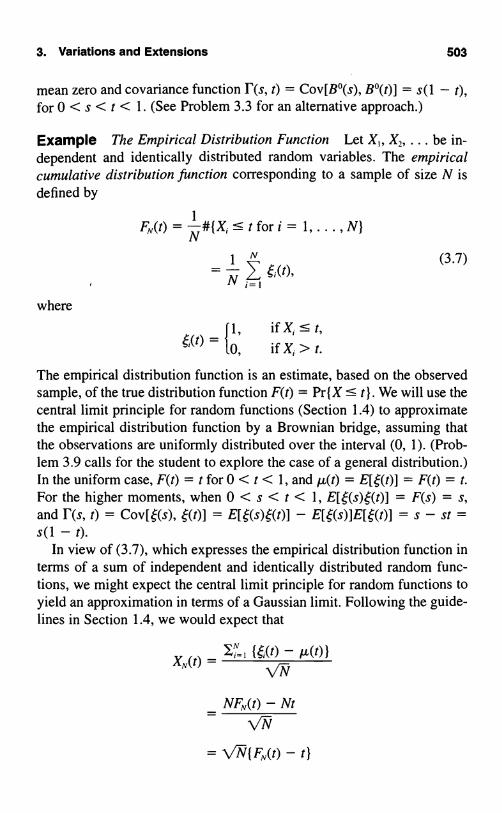
3. Variations and Extensions 503
mean zero and covariance function IF(s, t) = Cov[B°(s), B°(t)] = s(1 - t),for 0 < s < t < 1. (See Problem 3.3 for an alternative approach.)
Example The Empirical Distribution Function Let X, X,, ... be in-dependent and identically distributed random variables. The empiricalcumulative distribution function corresponding to a sample of size N isdefined by
Fn,(t) = N#{X; ---- t for i = 1, ... , N}
(3.7)
where
_ 1, ifX;<_t,'(t)
10, if X; > t.
The empirical distribution function is an estimate, based on the observedsample, of the true distribution function F(t) = Pr{X < t). We will use thecentral limit principle for random functions (Section 1.4) to approximatethe empirical distribution function by a Brownian bridge, assuming thatthe observations are uniformly distributed over the interval (0, 1). (Prob-lem 3.9 calls for the student to explore the case of a general distribution.)In the uniform case, F(t) = t for 0 < t < 1, and µ(t) = E[t;(t)] = F(t) = t.For the higher moments, when 0 < s < t < 1, F(s) = s,and I'(s, t) = fi(t)] = E[6(s)4(t)] - s - st =s(1 - t).
In view of (3.7), which expresses the empirical distribution function interms of a sum of independent and identically distributed random func-tions, we might expect the central limit principle for random functions toyield an approximation in terms of a Gaussian limit. Following the guide-lines in Section 1.4, we would expect that
XN(t)_" {;(t) - A(t))
VN-
NF,,, (t) - Nt
VN
= \{FN(t) - t}

504 VIII Brownian Motion and Related Processes
would converge, in an appropriate sense, to a Gaussian process with zeromean and covariance I'(s, t) = s(1 - t), for 0 < s < t < 1. As we havejust seen, this process is a Brownian bridge. Therefore, we would expectthe approximation
Such approximations are heavily used in the theory of nonparametricstatistics.
3.4. Brownian Meander
Brownian meander {B+(t); t ? 0} is Brownian motion conditioned to bepositive. Recall (3.3) and (3.5):
G,(x, y) = Pr{B(t) > y, B(u) > OIB(0) = x}
- D(,) 4)(Y-X),Vso that
G,(x, 0) = B(u) > OIB(O) = x}
_(D(Vt)(D(It -N-X)
The transition law for Brownian meander is
Pr{B+(t) > yIB+(0) = x) = Pr(B(t) > B(u) > 0, B(0) = x},
whence
Pr{B+(t) > yIB+(0) = x} = G,(x, y)G,(x, 0)
4)(y + x) - 4)(y
-Vx)
(D( t) - (D(t)

3. Variations and Extensions 505
Of most interest is the limiting case as x -> 0,
(D(y+x)0(y X)
Pr{B+(t) > yIB+(0) = 0} = lim (x 1 - ( xlX0 v
0(0)
= e
A simple integration yields the mean00
E[B+(t)IB+(0) = 01 = J Pr{B+(t) > YIB+(0) = 0} dy0
x=J dy
0
00
= z e dyf 1 -+ '_x
Exercises
3.1. Show that the cumulative distribution function for reflected Brown-ian motion is
Pr{R(t) < yIR(0) = x} _(YX) - (D X)
_ (D(yN/t-xl + (D(Yx l - 1
(x + Y (X_ Y-7t-) - 4 -7t-).
Evaluate this probability when x = 1, y = 3, and t = 4.
506 VIII Brownian Motion and Related Processes
3.2. The price fluctuations of a share of stock of a certain company arewell described by a Brownian motion process. Suppose that the companyis bankrupt if ever the share price drops to zero. If the starting share priceis A(0) = 5, what is the probability that the company is bankrupt at timet = 25? What is the probability that the share price is above 10 at timet = 25?
3.3. The net inflow to a reservoir is well described by a Brownian mo-tion. Because a reservoir cannot contain a negative amount of water, wesuppose that the water level R(t) at time t is a reflected Brownian motion.What is the probability that the reservoir contains more than 10 units ofwater at time t = 25? Assume that the reservoir has unlimited capacity andthat R(0) = 5.
3.4. Suppose that the net inflows to a reservoir follow a Brownian mo-tion. Suppose that the reservoir was known to be empty 25 time units agobut has never been empty since. Use a Brownian meander process to eval-uate the probability that there is more than 10 units of water in the reser-voir today.
3.5. Is reflected Brownian motion a Gaussian process? Is absorbedBrownian motion (cf. Section 1.4)?
Problems
3.1. Let B,(t) and B,(t) be independent standard Brownian motionprocesses. Define
R(t) = B,(t)2 + B,(t)2, t ? 0.
R(t) is the radial distance to the origin in a two-dimensional Brownian mo-tion. Determine the mean of R(t).
3.2. Let B(t) be a standard Brownian motion process. Determine theconditional mean and variance of B(t), 0 < t < 1, given that B(1) = b.
3.3. Let B(t) be a standard Brownian motion. Show that B(u) - uB(1),0 < u < 1, is independent of B(1).

Problems 507
(a) Use this to show that B°(t) = B(t) - tB(1), 0 s t < 1, is a Brown-ian bridge.
(b) Use the representation in (a) to evaluate the covariance function fora Brownian bridge.
3.4. Let B(t) be a standard Brownian motion. Determine the covariancefunction for
WI(s) = (1 - s)B(s
1- s), 0 < s < 1,
and compare it to that for a Brownian bridge.
3.5. Determine the expected value for absorbed Brownian motion A(t)at time t = 1 by integrating the transition density (3.6) according to
x
E[A(1)IA(0) = x] = f y p(y, 1Ix) dy0x
= f y[(k(y - x) - 4(y + x)] dy.0
The answer is E[A(1)IA(0) = x] = x. Show that E[A(t)IA(0) = x] = x forall t > 0.
3.6. Let M = max{A(t); t 0} be the largest value assumed by an ab-sorbed Brownian motion A(t). Show that Pr{M > zIA(0) = x} = x/z for0<x<z.
3.7. Let to = 0 < t, < t2 < ... be time points, and define X,, = A(t,,),where A(t) is absorbed Brownian motion starting from A(0) = x. Showthat is a nonnegative martingale. Compare the maximal inequality(5.7) in II with the result in Problem 3.6.
3.8. Show that the transition densities for both reflected Brownian mo-tion and absorbed Brownian motion satisfy the diffusion equation (1.3) inthe region 0 < x < oo.
3.9. Let F(t) be a cumulative distribution function and B°(u) a Brown-ian bridge.

508 VIII Brownian Motion and Related Processes
(a) Determine the covariance function for B°(F(t)).(b) Use the central limit principle for random functions to argue that
the empirical distribution functions for random variables obeyingF(t) might be approximated by the process in (a).
4. Brownian Motion with Drift
Let {B(t); t ? 0) be a standard Brownian motion process, and let µ ando, > 0 be fixed. The Brownian motion with drift parameter µ and varianceparameter 0-22 is the process
X(t) = µt + o-B(t) for t ? 0. (4.1)
Alternatively, Brownian motion with drift parameter µ and variance para-meter o-2 is the process whose increments over disjoint time intervals areindependent (property (b) of the definition of standard Brownian motion)and whose increments X(t + s) - X(t), t, s > 0, are normally distributedwith mean ps and variance o-2s. When X(0) = x, we have
Pr{X(t) : yIX(0) = x) = Pr{µt + oB(t) : ylo-B(0) = x}
= Pr j B(t) c Yo µt I = o-I
=4CDr(y
Crµt)=(D(y µt).
Brownian motion with drift is not symmetric when µ 0 0, and the reflec-tion principle cannot be used to compute the distribution of the maximumof the process. We will use an infinitesimal first step analysis to determinesome properties of Brownian motion with drift. To set this up, let us in-troduce some notation to describe changes in the Brownian motion withdrift over small time intervals of length At. We let OX = X(t + At) - X(t)and AB = B(t + At) - B(t). Then AX = µ0t + o-AB, and
X(t + At) = X(t) + AX = X(t) + µ0t + o-AB. (4.2)
We observe that the conditional moments of AX, given X(t) = x, are
E[AXIX(t) = x] = µ0t + o-E[AB] = µ0t, (4.3)
Var[OXIX(t) = x] = 0-2E[(AB)2] = o-2At, (4.4)

4. Brownian Motion with Drift 509
and
2Ot + ( 0t)22 =] _ 20t +AX 2I X(t) = t1t)E 4 5[( ) µx o o o( , ( . )
while
E[(1 X)`] = o(At) for c > 2. (4.6)
4.1. The Gambler's Ruin Problem
Let us suppose that X(O) = x, and that a < x and b > x are fixed quanti-ties. We will be interested in some properties of the random time T atwhich the process first assumes one of the values a or b. This so-called hit-ting time is formally defined by
T=Tub=min(t? 0;X(t)=aorX(t)=b}.Analogous to the gambler's ruin problem in a random walk (III, Section5.3), we will determine the probability that when the Brownian motionexits the interval (a, b), it does so at the point b. The solution for a stan-dard Brownian motion was obtained in Section 1 by using the invarianceprinciple. Here we solve the problem for Brownian motion with drift byinstituting an infinitesimal first step analysis.
Theorem 4.1 For a Brownian motion with drift parameter µ and vari-ance parameter Q2, and a < x < b,
u(x) = Pr{X(T,,,) = bjX(0) = x} =e-2gda2 - e-2"'°2
e-2,.bla22 _ e-2p,,/o2 . (4.7)
Proof Our proof is not entirely complete in that we will assume (i) thatu(x) is twice continuously differentiable, and (ii) that we can choose atime increment At so small that exiting the interval (a, b) prior to time Atcan be neglected. With these provisos, at time At the Brownian motionwill be at the position X(0) + .X = x + OX, and the conditional proba-bility of exiting at the upper point b is now u(x + AX). Invoking the lawof total probability, it must be that u(x) = Pr{X(T) = b1X(0) = x) =E[Pr{X(T) = bIX(0) = x, X(At) = x + OX}IX(0) = x] = E[u(x + OX)],where a < x < b.

510 Vlll Brownian Motion and Related Processes
The next step is to expand u(x + AX) in a Taylor series, wherebyu(x + = u(x) + u'(x)AX + ZU''(x)(AX)2 + o(AX)2. Then
u(x) = E[u(x + AX)]
= u(x) + u'(x)E[AX] + 2'u'"(x)E[(OX)2] + E[o(At)].
We use (4.3), (4.5), and (4.6) to evaluate the moments of AX, obtaining
u(x) = u(x) + u'(x)AAt + ;u'"(x)O'At + o(At),
which, after subtracting u(x), dividing by At, and letting At -* 0, becomesthe differential equation
0 = µu'(x) + ;o_2u"(x) for a < x < b. (4.8)
The solution to (4.8) is
u(x) = Ae_21) °z + B,
where A and B are constants of integration. These constants are deter-mined by the conditions u(a) = 0 and u(b) = 1. In words, the probabilityof exiting at b if the process starts at a is zero, while the probability of ex-iting at b if the process starts at b is one. When these conditions are usedto determine A and B, then (4.7) results.
Example Suppose that the fluctuations in the price of a share of stockin a certain company are well described by a Brownian motion with driftµ = 1/10 and variance 0-22 = 4. A speculator buys a share of this stock ata price of $100 and will sell if ever the price rises to $110 (a profit) ordrops to $95 (a loss). What is the probability that the speculator sells at aprofit? We apply (4.7) with a = 95, x = 100, b = 110, and 2µ/o22 _2(0.1)/4 = 1/20. Then
e-100/20 - e-95/20
Pr(Sell at profit) = = 0.419.e-na2o - e-9sao
The Mean Time to Exit an Interval
Using another infinitesimal first step analysis, the mean time to exit an in-terval may be determined for Brownian motion with drift.

4. Brownian Motion with Drift 511
Theorem 4.2 For a Brownian motion with drift parameter /.Land vari-ance parameter o-Z, and a < x < b,
E[T,,,>I X(0) = x] = 1[u(x)(b - a) - (x - a)], (4.9)A
where u(x) is given in (4.7).
Proof Let v(x) = E[TT,,,IX(0) = x]. As in the proof of Theorem 4.1, wewill assume (i) that v(x) is twice continuously differentiable, and (ii) thatwe can choose a time increment At so small that exiting the interval (a, b)prior to time At can be neglected. With these provisos, after time At theBrownian motion will be at the position X(O) + AX = x + AX, and theconditional mean time to exit the interval is now At + v(x + AX). Invok-ing the law of total probability, it must be that v(x) = E[TI X(0) = x] =E[At + E{T - AtIX(0) = x, X(At) = x + AX}IX(0) = x] = At +E[v(x + AX)], where a < x < b.
The next step is to expand v(x + .X) in a Taylor series, wherebyv(x + X) = v(x) + v'(x)OX + ;v''(x)(OX)' + o(OX)'. Then
v(x) = At + E[v(x + AX)]
= At + v(x) + v'(x)E[AX] + Zv'"(x)E[(zXX)2] + E[o(OX)2].
We use (4.3), (4.5), and (4.6) to evaluate the moments of AX, obtaining
v(x) = At + v(x) + v'(x)AAt + ;v"(x)o-2At + o(At),
which, after subtracting v(x), dividing by At, and letting At - 0, becomesthe differential equation
-1 = pv'(x) + ;cr2v"(x) for a < x < b. (4.10)
Since it takes no time to reach the boundary if the process starts at theboundary, the conditions are v(a) = v(b) = 0. Subject to these conditions,the solution to (4.10) is uniquely given by (4.9), as is easily verified (Prob-lem 4.1).
Example A Sequential Decision Procedure A Brownian motion X(t)either (i) has drift p. = +;5 > 0, or (ii) has drift µ = - S < 0, and it isdesired to determine which is the case by observing the process. The

512 VIII Brownian Motion and Related Processes
process will be monitored until it first reaches the level b > 0, in whichcase we will decide that the drift is µ = +18, or until it first drops to thelevel a < 0, which occurrence will cause us to decide in favor of µ = -ZS.This decision procedure is, of course, open to error, but we can evaluatethese error probabilities and choose a and b so as to keep the error proba-bilities acceptably small. We have
a = Pr{Decide µ = -ZS}
= Pr{X(T) = bI E[X(t)] = -2'5t}(4.11)
1 - e+woz
= e+s' 2 _ e+&,' 2 (using (4.7))
and
1 - /3 = Pr{Decide µ = +2Sµ = +25}
= Pr{X(T) = bIE[X(t)] =+2 6t} (4.12)
_ 1 - e-&-''p2- e-w-2 - e-&,/v
If acceptable levels of the error probabilities a and /3 are prescribed, thenwe can solve in (4.11) and (4.12) to determine the boundaries to be usedin the decision procedure. The reader should verify that these boundariesare
a 8 log(1 aand b = 8 log(1a
R). (4.13)
For a numerical example, if 0,2 = 4 and we are attempting to decide be-tween µ = -2 and µ = +2, and the acceptable error probabilities are cho-sen to be a = 0.05 and /3 = 0.10, then the decision boundaries that shouldbe used are a = -4 log(0.95/0.10) = -9.01, and b = 4 log(0.90/0.05)11.56.
In the above procedure for deciding the drift of a Brownian motion, theobservation duration until a decision is reached will be a random variablewhose mean will depend upon the true value of the drift. Using (4.9) withx = 0 and µ replaced by ±15 gives us the mean observation interval, as afunction of the true mean µ:
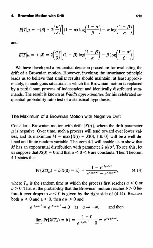
4. Brownian Motion with Drift 513
E[TI p. = -ZS] = 2(S) [(1 - a) log(' -a
and
- a log
E[TItk = +ZS] =2(S)z[(1
- R)log(1
a R) - R log(' a2
We have developed a sequential decision procedure for evaluating thedrift of a Brownian motion. However, invoking the invariance principleleads us to believe that similar results should maintain, at least approxi-mately, in analogous situations in which the Brownian motion is replacedby a partial sum process of independent and identically distributed sum-mands. The result is known as Wald's approximation for his celebrated se-quential probability ratio test of a statistical hypothesis.
The Maximum of a Brownian Motion with Negative Drift
Consider a Brownian motion with drift {X(t)}, where the drift parameterµ is negative. Over time, such a process will tend toward ever lower val-ues, and its maximum M = max { X(t) - X(0); t ? 0) will be a well-de-fined and finite random variable. Theorem 4.1 will enable us to show thatM has an exponential distribution with parameter 21µI/o.2. To see this, letus suppose that X(0) = 0 and that a < 0 < b are constants. Then Theorem4.1 states that
Pr{X(Tb) = bI X(0) = x} =1 - e-zpd°z
e-10m2 _ e-z,°i°z, (4.14)
where is the random time at which the process first reaches a < 0 orb > 0. That is, the probability that the Brownian motion reaches b > 0 be-fore it ever drops to a < 0 is given by the right side of (4.14). Becauseboth µ<0and a<0,then aµ>0and
e`W,1J ' = e-'- ''°` --> 0 as a - -oo, and then
-zpbi°zlim Pr{X(Tnb) = b) = 1 -0 = ee-zpei°2 _ 0

514 VIII Brownian Motion and Related Processes
But as a - -oo, the left side of (4.14) becomes the probability that theprocess ever reaches the point b, that is, the probability that the maximumM of the process ever exceeds b. We have deduced, then, the desired ex-ponential distribution
Pr(M>b) =e'µ1°' b > 0. (4.15)
4.2. Geometric Brownian Motion
A stochastic process (Z(t); t ? 0) is called a geometric Brownian motionwith drift parameter a if X(t) = log Z(t) is a Brownian motion with drift
a - io2 and variance parameter a-2. Equivalently, Z(t) is geometricBrownian motion starting from Z(0) = z if
Z(t) = Zex(t) = ze(n- v-)r+oe(nl 1 , (4.16)
where B(t) is a standard Brownian motion starting from B(0) = 0.Modern mathematical economists usually prefer geometric Brownian
motion over Brownian motion as a model for prices of assets, say sharesof stock, that are traded in a perfect market. Such prices are nonnegativeand exhibit random fluctuations about a long-term exponential decay orgrowth curve. Both of these properties are possessed by geometricBrownian motion, but not by Brownian motion itself. More importantly,if to < t, < < t are time points, then the successive ratios
Z(t,) Z(t) Z(t)Z(t,,-,)
are independent random variables, so that crudely speaking, the percent-age changes over nonoverlapping time intervals are independent.
We turn to determining the mean and variance of geometric Brownianmotion. Let 6 be a normally distributed random variable with mean zeroand variance one. We begin by establishing the formula
E[e"{]=e="2, -x<A<oo,
which results immediately from
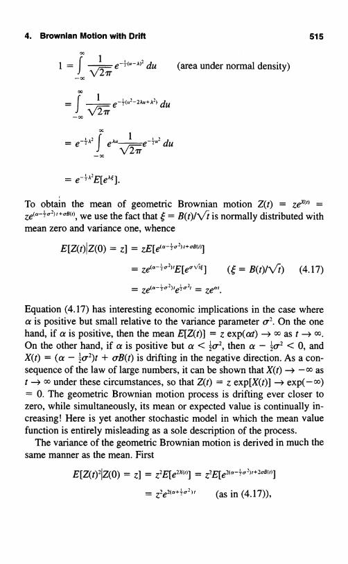
4. Brownian Motion with Drift 515
x
1 = j 12 du (area under normal density)
-x
=J
1 e av'-zau+A' du11
-x
X
= e- AZ r e"" 1 e- 112 du1 N /5_1-x
=
To obtain the mean of geometric Brownian motion Z(t) = ze"' _zee°-=°2''+°ac", we use the fact that = B(t)/ is normally distributed with
mean zero and variance one, whence
E[Z(t)I Z(0) = z] = zE[e(«_°-)1+°e(I)]
= Ze(« a2),E[e°"I"'] ( = B(t)lN17) (4.17)
7 at
Equation (4.17) has interesting economic implications in the case wherea is positive but small relative to the variance parameter .2 On the onehand, if a is positive, then the mean E[Z(t)] = z exp(at) -4 oo as t - oo.On the other hand, if a is positive but a < ZO.2, then a - ;Q.2 < 0, andX(t) = (a - 20 2)t + QB(t) is drifting in the negative direction. As a con-sequence of the law of large numbers, it can be shown that X(t) - -00 ast - oo under these circumstances, so that Z(t) = z exp[X(t)] - exp(-cc)= 0. The geometric Brownian motion process is drifting ever closer tozero, while simultaneously, its mean or expected value is continually in-creasing! Here is yet another stochastic model in which the mean valuefunction is entirely misleading as a sole description of the process.
The variance of the geometric Brownian motion is derived in much thesame manner as the mean. First
E[Z(t)2IZ(0) = Z] = z2E[e211t) ] = z2E[e2c« °'-1,+z°ao,]
= zzezc«+_°=,t (as in (4.17))

516 VIII Brownian Motion and Related Processes
and then
Var[Z(t)] = E[Z(t)2] - { E[Z(t)] } 2
e2(a+-a2), - z2e2at= Z2 (4.18)
= Z2e2at(e(' 2, - 1).
Because of their close relation as expressed in the definition (4.16), manyresults for Brownian motion can be directly translated into analogous re-sults for geometric Brownian motion. For example, let us translate thegambler's ruin probability in Theorem 4.1. For A < 1 and B > 1, define
T=TA.a=minjt?0; Z(t) =AorZ(t) =BI.
Theorem 4.3 For a geometric Brownian motion with drift parametera and variance parameter or, and A < 1 < B,
PrIZ(T) =1
=1 - A'-2ada:
(4.19)BB1-2aha2 - A'-2aia2
.19)
Example Suppose that the fluctuations in the price of a share of stockin a certain company are well described by a geometric Brownian motionwith drift a = 1/10 and variance o2 = 4. A speculator buys a share of thisstock at a price of $100 and will sell if ever the price rises to $110(a profit) or drops to $95 (a loss). What is the probability that the spec-ulator sells at a profit? We apply (4.19) with A = 0.95, B = 1.10 and1 - 2a/o-2 = 1 - 2(0.1)/4 = 0.95. Then
Pr{Sell at profit} =I - 0.95095 = 0.3342.
1.100.91 - 0.950.95
Example The Black-Scholes Option Pricing Formula A call, or war-rant, is an option entitling the holder to buy a block of shares in a givencompany at a specified price at any time during a stated interval. Thus thecall listed in the financial section of the newspaper as
Hewlett Aug $60 $6
means that for a price of $6 per share, one may purchase the privilege (op-tion) of buying the stock of Hewlett-Packard at a price of $60 per share at

4. Brownian Motion with Drift 517
any time between now and August (by convention, always the third Fridayof the month). The $60 figure is called the striking price. Since the mostrecent closing price of Hewlett was $59, the option of choosing when tobuy, or not to buy at all, carries a premium of $7 = $60 + $6 - $59 overa direct purchase of the stock today.
Should the price of Hewlett rise to, say, $70 between now and the thirdFriday of August, the owner of such an option could exercise it, btlying atthe striking price of $60 and immediately selling at the then current mar-ket price of $70 for a $10 profit, less, of course, the $6 cost of the optionitself. On the other hand, should the price of Hewlett fall, the optionowner's loss is limited to his $6 cost of the option. Note that the seller(technically called the "writer") of the option has a profit limited to the $6that he receives for the option but could experience a huge loss should theprice of Hewlett soar, say to $100. The writer would then either have togive up his own Hewlett shares or buy them at $100 on the open marketin order to fulfill his obligation to sell them to the option holder at $60.
What should such an option be worth? Is $6 for this privilege a fairprice? While early researchers had studied these questions using a geo-metric Brownian motion model for the price fluctuations of the stock, theyall assumed that the option should yield a higher mean return than themean return from the stock itself because of the unlimited potential risk tothe option writer. This assumption of a higher return was shown to be falsein 1973 when Fisher Black, a financial consultant with a Ph.D. in appliedmathematics, and Myron Scholes, an assistant professor in finance at MIT,published an entirely new and innovative analysis. In an idealized settingthat included no transaction costs and an ability to borrow or lend limit-less amounts of capital at the same fixed interest rate, they showed that anowner, or a writer, of a call option could simultaneously buy or sell the un-derlying stock ("program trading") in such a way as to exactly match thereturns of the option. Having available two investment opportunities withexactly the same return effectively eliminates all risk, or randomness, byallowing an investor to buy one while selling the other. The implicationsof their result are many. First, since writing an option potentially carriesno risk, its return must be the same as that for other riskless investmentsin the economy. Otherwise, limitless profit opportunities bearing no riskwould arise. Second, since owning an option carries no risk, one shouldnot exercise it early, but hold it until its expiration date, when, if the mar-ket price exceeds the striking price, it should be exercised, and otherwise

518 VIII Brownian Motion and Related Processes
not. These two implications then lead to a third, a formula that establishedthe worth, or value, of the option.
The Black-Scholes paper spawned hundreds, if not thousands, of fur-ther academic studies. At the same time, their valuation formula quicklyinvaded the financial world, where soon virtually all option trades weretaking place at or near their Black-Scholes value. It is remarkable that thevaluation formula was adopted so quickly in the real world in spite of theesoteric nature of its derivation and the ideal world of its assumptions.
In order to present the Black-Scholes formula, we need some notation.Let S(t) be the price at time t of a share of the stock under study. We as-sume that S(t) is described by a geometric Brownian motion with drift pa-rameter a and variance parameter o=. Let F(z, T) be the value of an option,where z is the current price of the stock and r is the time remaining untilexpiration. Let a be the striking price. When r = 0, and there is no timeremaining, one exercises the option for a profit of z - a if z > a (marketprice greater than striking price) and does not exercise the option, but letsit lapse, or expire, if z : a. This leads to the condition
F(z,0)=(z-a)+=max{z-a,0}.
The Black-Scholes analysis resulted in the valuation
F(z, T) = e-ME[(Z(T) - a)+IZ(0) = z], (4.20)
where r is the return rate for secure, or riskless, investments in the econ-omy, and where Z(t) is a second geometric Brownian motion having driftparameter r and variance parameter o . Looking at (4.20), the carefulreader will wonder whether we have made a mistake. No, the worth of theoption does not depend on the drift parameter a of the underlying stock.
In order to put the valuation formula into a useful form, we write
Z(T) = zee`- B(T)/N//T, (4.21)
and observe that
ze O )T+O\'Tf >a
is the same as
20' T> vo =
dVI-T(4.22)

4. Brownian Motion with Drift 519
Then
erTF(z, T) = E[(Z(T) - a)+IZ(0) = z]
= E[(ze'r-'?2)T+OV'Tf - a)+l
W
= J [ze`,.-' u',-+ox/-n_ - al O(v) dv.
Vox x
e'2 'T J e°","O(v) dv - a J 4(v) dv.V0 V0
Completing the square in the form
-;v'+0- v= -![(v-0-)Z20-27]N/IT
shows that
whence
ean4(v) = e+°'-4(v - 0-v"T) ,
x
errF(z, T) =ze(r
J 4(v - 0-V T) dv - a[1 - (D(vo)l0-o
= zer-[1 - 4 (vo - 0-V T)l - a[1 - F(vo)].
Finally, note that
--log(a/z) - (r + ;0-22)7
"" //0-o- UVT=
and that
0-V
1 - I(x) = I(-x) and log(a/z) = -log(z/a)
to get, after multiplying by e-r-, the end result
flog(z/a) + (r + Zoz)T
lF(z, r) = z4l/
(4.23)log(z/a) + (r - Z0-')
O'

520 VIII Brownian Motion and Related Processes
Equation (4.23) is the Black-Scholes valuation formula. Four of the fivefactors that go into it are easily and objectively evaluated: The currentmarket prize z, the striking price a, the time r until the option expires, andthe rate r of return from secure investments such as short-term govern-ment securities. It is the fifth factor, a., sometimes called the volatility, thatpresents problems. It is, of course, possible to estimate this parameterbased on past records of price movements. However, it should be empha-sized that it is the volatility in the future that will affect the profitability ofthe option, and when economic conditions are changing, past history maynot accurately indicate the future. One way around this difficulty is towork backwards and use the Black-Scholes formula to impute a volatilityfrom an existing market price of the option. For example, theHewlett-Packard call option that expires in August, six months or, T = 2year, in the future, with a current price of Hewlett-Packard stock of $59,a striking price of $60, and secure investments returning aboutr = 0.05, a volatility of a. = 0.35 is consistent with the listed option price
StrikingTime to
Expiration Black-ScholesPrice (Years) Offered Valuation
a T Price F(z, T)
130 1/12 $17.00 $17.45130 2/12 19.25 18.87135 1/12 13.50 13.09135 2/12 15.13 14.92140 1/12 8.50 9.26140 2/12 12.00 11.46
145 1/12 5.50 6.14145 2/12 9.13 8.52145 5/12 13.63 13.51
150 1/12 3.13 3.80150 2/12 6.38 6.14155 1/12 1.63 2.18155 2/12 4.00 4.28155 5/12 9.75 9.05

Exercises 521
of $6. (When o = 0.35 is used in the Black-Scholes formula, the result-ing valuation is $6.03.) A volatility derived in this manner is called an im-puted or implied volatility. Someone who believes that the future will bemore variable might regard the option at $6 as a good buy. Someone whobelieves the future to be less variable than the imputed volatility ofo, = 0.35 might be inclined to offer a Hewlett-Packard option at $6.
The table on the previous page compares actual offering prices on Feb-ruary 26, 1997, for options in IBM stock with their Black-Scholes valua-tion using (4.23). The current market price of IBM stock is $146.50, andin all cases, the same volatility a = 0.30 was used.
The agreement between the actual option prices and their Black-Scholes valuations seems quite good.
Exercises
4.1. A Brownian motion {X(t)} has parameters µ = -0.1 and a- = 2.What is the probability that the process is above y = 9 at time t = 4, giventhat it starts at x = 2.82?
4.2. A Brownian motion {X(t)} has parameters µ = 0.1 and a- = 2.Evaluate the probability of exiting the interval (a, b] at the point b start-ing from X(0) = 0 for b = 1, 10, and 100 and a = -b. Why do the prob-abilities change when alb is the same in all cases?
4.3. A Brownian motion {X(t)} has parameters µ = 0.1 and a = 2.Evaluate the mean time to exit the interval (a, b] from X(0) = 0 for b =1, 10, and 100 and a = -b. Can you guess how this mean time varies withb for b large?
4.4. A Brownian motion X(t) either (i) has drift p. = +16 > 0, or (ii) hasdrift µ = -ZS < 0, and it is desired to determine which is the case by ob-serving the process for a fixed duration T. If X(T) > 0, then the decisionwill be that µ = +ZS; If X(T) :5 0, then µ = -ZS will be stated. Whatshould be the length T of the observation period if the design error proba-bilities are set at a = 8 = 0.05? Use S = 1 and a- = 2. Compare this fixedduration with the average duration of the sequential decision plan in theexample of Section 4.1.
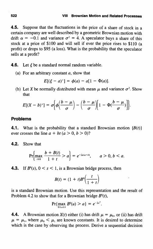
522 VIII Brownian Motion and Related Processes
4.5. Suppose that the fluctuations in the price of a share of stock in acertain company are well described by a geometric Brownian motion withdrift a = -0.1 and variance cr-2 = 4. A speculator buys a share of thisstock at a price of $100 and will sell if ever the price rises to $110 (aprofit) or drops to $95 (a loss). What is the probability that the speculatorsells at a profit?
4.6. Let be a standard normal random variable.
(a) For an arbitrary constant a, show that
E[(e - a)+] = 4(a) - a[1 - 4)(a)]
(b) Let X be normally distributed with mean µ and variance cr2. Showthat
E[(X - b)+] =+(1) - (b µ)L1 - (D(b
0" o v .1
Problems
4.1. What is the probability that a standard Brownian motion {B(t) }ever crosses the line a + bt (a > 0, b > 0)?
4.2. Show that
b + B(t)P = -> b<>0a e ,rmax 1+t a a.,
4.3. If B°(s), 0 < s < 1, is a Brownian bridge process, then
B(t) = (1 + t)B°( t )1+tis a standard Brownian motion. Use this representation and the result ofProblem 4.2 to show that for a Brownian bridge B°(t),
Pr{max B°(u) > a} = e-°'.°:511s1
4.4. A Brownian motion X(t) either (i) has drift µ = µ0i or (ii) has driftµ = µ,, where µ.° < µ, are known constants. It is desired to determinewhich is the case by observing the process. Derive a sequential decision

Problems 523
procedure that meets prespecified error probabilities a and 0. Hint: Baseyour decision on the process X'(t) = X(t) - ;(µo + µ,).
4.5. Change a Brownian motion with drift X(t) into an absorbed Brown-ian motion with drift X(t) by defining
XA(t) =(X(t), for t < r,0, fort? T,
where
T = min{t ? 0; X(t) = 0).
(We suppose that X(0) = x > 0 and that A < 0, so that absorption is sureto occur eventually.) What is the probability that the absorbed Brownianmotion ever reaches the height b > x?
4.6. What is the probability that a geometric Brownian motion with driftparameter a = 0 ever rises to more than twice its initial value? (You buystock whose fluctuations are described by a geometric Brownian motionwith a = 0. What are your chances to double your money?)
4.7. A call option is said to be "in the money" if the market price of thestock is higher than the striking price. Suppose that the stock follows ageometric Brownian motion with drift a, variance a2 , and has a currentmarket price of z. What is the probability that the option is in the moneyat the expiration time T? The striking price is a.
4.8. Verify the Hewlett-Packard option valuation of $6.03 stated in thetext when T = ;, z = $59, a = 60, r = 0.05 and a- = 0.35. What is theBlack-Scholes valuation if o- = 0.30?
4.9. Let r be the first time that a standard Brownian motion B(t) startingfrom B(0) = x > 0 reaches zero. Let A be a positive constant. Show that
w(x) = E[e-ATIB(0) = x] = e-'-21*.
Hint: Develop an appropriate differential equation by instituting aninfinitesimal first step analysis according to
w(x) = E[E{e-ATjB(Ot)}!B(0) = x] = E[e-A°'w(x + AB)].

524 VIII Brownian Motion and Related Processes
4.10. Let to = 0 < t, < t, < ... be time points, and define X = Z(t,,)where Z(t) is geometric Brownian motion with drift parameters
r and variance parameter 022 (see the geometric Brownian motion in theBlack-Scholes formula (4.20)). Show that is a martingale.
5. The Ornstein-Uhlenbeck Process*
The Ornstein-Uhlenbeck process {V(t); t ? 0 } has two parameters, a driftcoefficient (3 > 0 and a diffusion parameter 0-22. The process, starting fromV(0) = v, is defined in terms of a standard Brownian motion {B(t) } byscale changes in both space and time:
`V(t) = ve-O' +
aeB(e2a' - 1), fort ? 0. (5.1)
The first term on the right of (5.1) describes an exponentially decreasingtrend towards the origin. The second term represents the fluctuationsabout this trend in terms of a rescaled Brownian motion. The Orn-stein-Uhlenbeck process is another example of a continuous-state-space,continuous-time Markov process having continuous paths, inheritingthese properties from the Brownian motion in the representation (5.1). Itis a Gaussian process (see the discussion in Section 1.4), and (5.1) easilyshows its mean and variance to be
E[V(t)I V(0) = v] = ve-a', (5.2)
and
Var V(t)Vv2
[ (0) = x] = 2R Var[B(e2a' - 1)]
(5.3)
= 2( 1
ZR
Knowledge of the mean and variance of a normally distributed randomvariable allows its cumulative distribution function to be written in termsof the standard normal distribution (1.6), and by this means we can im-
This section contains material of a more specialized nature.

S. The Ornstein-Uhlenbeck Process 525
mediately express the transition distribution for the Ornstein-Uhlenbeckprocess as
V -2,8(y - xe 0`) lPr(V(t) y1V(0) = x} = ID( aV-l - e_20, I. (5.4)
The Covariance Function
Suppose that 0 < u < s, and that V(0) = x. Upon subtracting the mean asgiven by (5.2), we obtain
Cov[V(u), V(s)] = E[{V(u) - xe-Al) {V(s) - xe-g''}]
= 2Re-r,,+'''E[{B(e''-m" - 1)}{B(e'' - 1) }]
0,2
2
0,_ enc., a_e216
5.1. A Second Approach to Physical Brownian Motion
(5.5)
The path that we have taken to introduce the Ornstein-Uhlenbeck processis not faithful to the way in which the process came about. To begin an ex-planation, let us recognize that all models of physical phenomena have de-ficiencies, and the Brownian motion stochastic process as a model for theBrownian motion of a particle is no exception. If B(t) is the position of apollen grain at time t and if this position is changing over time, then thepollen grain must have a velocity. Velocity is the infinitesimal change inposition over infinitesimal time, and where B(t) is the position of thepollen grain at time t, the velocity of the grain would be the derivativedB(t)/dt. But while the paths of the Brownian motion stochastic processare continuous, they are not differentiable. This remarkable statement isdifficult to comprehend. Indeed, many elementary calculus explanationsimplicitly tend to assume that all continuous functions are differentiable,and if we were to be asked to find an example of one that wasn't, we might
526 VIII Brownian Motion and Related Processes
consider it quite a challenge. Yet each path of a continuous Brownian mo-tion stochastic process is (with probability one) differentiable at no point.We have encountered yet another intriguing facet of stochastic processesthat we cannot treat in full detail but must leave for future study. We willattempt some motivation, however. Recall that the variance of the Brown-ian increment AB is At. But variations in the normal distribution are notscaled in terms of the variance, but in terms of its square root, the standarddeviation, so that the Brownian increment AB is roughly on the order of\, and the approximate derivative
AB AB 1
At V VA-t
is roughly on the order of 1/\. This, of course, becomes infinite asAt -, 0, which suggests that a derivative of Brownian motion, were it toexist, could only take the values ±c. As a consequence, the Brownianpath cannot have a derivative. The reader can see from our attempt at ex-planation that the topic is well beyond the scope of an introductory text.
Although its movements may be erratic, a pollen grain, being a physi-cal object of positive mass, must have a velocity, and the Ornstein-Uhlenbeck process arose as an attempt to model this velocity directly.Two factors are postulated to affect the particle's velocity over a smalltime interval. First, the frictional resistance or viscosity of the surround-ing medium is assumed to reduce the magnitude of the velocity by adeterministic proportional amount, the constant of proportionality beingR > 0. Second, there are random changes in velocity caused by collisionswith neighboring molecules, the magnitude of these random changesbeing measured by a variance coefficient o-'-. That is, if V(t) is the veloc-ity at time t, and AV is the change in velocity over (t, t + At], we mightexpress the viscosity factor as
E[zVIV(t) = v] = -,6v1t + o(At) (5.6)
and the random factor by
Var[i VI V(t) = v] = o-2At + o(Ot). (5.7)
The Ornstein-Uhlenbeck process was developed by taking (5.6) and (5.7)together with the Markov property as the postulates, and from them de-riving the transition probabilities (5.4). While we have chosen not to fol-low this path, we will verify that the mean and variance given in (5.2) and

5. The Ornstein-Uhlenbeck Process 527
(5.3) do satisfy (5.6) and (5.7) over small time increments. Beginning with(5.2) and the Markov property, the first step is
E[V(t + ot)IV(t) = v] = ve-O-" = v[1 - 80t + o(Ot)],
and then
E[OVI V(t) = v] = E[V(t + At)I V(t) = v] - v
= -/3vAt + o(Ot),
and over small time intervals the mean change in velocity is the propor-tional decrease desired in (5.6). For the variance, we have
- Var[OVIV(t) = v] = Var[V(t + ot)IV(t) = v]
0-2(1-e2/3
= 0,2A t + o(Ot),
and the variance of the velocity increment behaves as desired in (5.7). Infact, (5.6) and (5.7) together with the Markov property can be taken as thedefinition of the Ornstein-Uhlenbeck process in much the same way, butinvolving far deeper analysis, that the infinitesimal postulates of V, Sec-tion 2.1 serve to define the Poisson process.
Example Tracking Error Let V(t) be the measurement error of a radarsystem that is attempting to track a randomly moving target. We assumeV(t) to be an Ornstein-Uhlenbeck process. The mean increment E[OVI V(t)= v] = -/3vtt + o(At) represents the controller's effort to reduce the cur-rent error, while the variance term reflects the unpredictable motion of thetarget. If /3 = 0.1, 0- = 2, and the system starts on target (v = 0), the prob-ability that the error is less than one at time t = 1 is, using (5.4),
Pr(IV(t)j<1)=211,
( 1- e I- e-)'-a
_20(1 I- e-0 2)) - q)( 20(1 1 e 12))
= D(0.53) - 1(-0.53) = 0.4038.

528 VIII Brownian Motion and Related Processes
As time passes, this near-target probability drops to I(1/N/,2-0-) -(D(-I/ N/-2-0) = F(0.22) - 4(-0.22) = 0.1742.
Example Genetic Fluctuations under Mutation In VI, Section 4, weintroduced a model describing fluctuations in gene frequency in a popula-tion of N individuals, each either of gene type a or gene type A. With X(t)being the number of type a individuals at time t, we reasoned that X(t)would be a birth and death process with parameters
A' -1 Nl LN(1Y) + (1 N)YZ]
and
µj=WNLN'Y] +(I-N)(I-Y2),.
The parameters y, and y2 measured the rate of mutation from a-type to A-type, and A-type to a-type, respectively. Here we attempt a simplified de-scription of the model when the population size N is large. The steady-state fluctuations in the relative gene frequency X(t)/N are centered on themean
Y2Ir =Y1 +y,
Accordingly, we define the rescaled and centered process
VN(t) = N/N_ (XN(t) - -rr).
With
AV= VN(t + At) - VN(t), and AX = X(t + At) - X(t),
we have
E[OXX(t) = j] = (A; - µ)0t + o(Ot),
which becomes, after substitution and simplification,
j- N y,lAt + o(Ot).E[.X(t) = j] = NA[(1 -
)

5. The Ornstein-Uhlenbeck Process 529
More tedious calculations show that
E[AX2IX(t) = j] = NA2y,Y2 +0L (y, + y,)2 (!N)1At-
Our next step is to rescale these in terms of v, using
J VN=1r+c.
In the rescaled variables,
E[AVIVN(t) = v] = IEI AXX(t) j v
N N=a+V
/ v= AVNV I 1 - IT - I yZ - (IT + v -) y, Ai + o(At)
K
= -A(y, + y2)VAt + o(Ot).
A similar substitution shows that
E[AV 2I VN(t) = v] =2AY,Y2
(Y, + y2)2 At + o(Ot).
Similar computations show that the higher moments of AV are negligible.Since the relations (5.6) and (5.7) serve to characterize the Ornstein-Uhlenbeck process, the evidence is compelling that the rescaledgene processes (VN(t)) will converge in some appropriate sense to anOrnstein-Uhlenbeck process V(t) with
=A(Y,+Y2) and o--_2AY,Y2
16
(Y, + Y2)
and
X(t) ~ Nir + \/NV(t) for large N.
This is indeed the case, but it represents another topic that we must leavefor future study.

530 VIII Brownian Motion and Related Processes
5.2. The Position Process
If V(t) is the velocity of the pollen grain, then its position at time t would be
S(t) = S(O) + f V(u) du. (5.8)0
Because the Ornstein-Uhlenbeck process is continuous, the integral in(5.8) is well-defined. The Ornstein-Uhlenbeck process is normally dis-tributed, and so is each approximating sum to the integral in (5.8). It mustbe, then, that the position process S(t) is normally distributed, and to de-scribe it, we need only evaluate its mean and covariance functions. Tosimplify the mathematics without losing any essentials, let us assume thatS(0) = V(0) = 0. Then
11
E[S(t)] = E Iff V(s) ds] = f E[V(s)] ds = 0.0 0
(The interchange of integral and expectation needs justification. Since theexpected value of a sum is always the sum of the expected values, the in-terchange of expectation with Riemann approximating sums is clearlyvalid. What is needed is justification in the limit as the approximatingsums converge to the integrals.)
rrr z1
Var[S(t)] = E[S(t)2] = E[ f V(s) ds}J0
= EI j f V(u) du 11 f V(s) ds }J0
0 J
Ir
= f f E[V(s)V(u)] du ds00
I S
= 2 f f E[V(s)V(u)] du ds (5.9)00
f S
= v2 f f e-kk'+10) du ds (Using (5.5))X00a12- f e-A'(O' - 1- I + e-P) dsp2
It11
_ zlt - (1 - e F') + R(1 - e '-R')J.

5. The Ornstein-Uhlenbeck Process 531
This variance behaves like that of a Brownian motion when t is large inthe sense that
Var[S(t)] v2- as t - .
t /3-
That is, observed over a long time span, the particle's position as n\odeledby an Ornstein-Uhlenbeck velocity behaves much like a Brownian mo-tion with variance parameter o-2//32. In this sense, the Ornstein-Uhlenbeckmodel agrees with the Brownian motion model over long time spans andimproves upon it for short durations. Section 5.4 offers another approach.
Example - Stock Prices It is sometimes assumed that the market priceof a share of stock follows the position process under an Ornstein-Uhlenbeck velocity. The model is consistent with the Brownian motionmodel over long time spans. In the short term, the price changes are notindependent but have an exponentially decreasing correlation meant tocapture some notion of a market momentum. Suppose a call option is tobe exercised, if profitable at a striking price of a, at some fixed time t inthe future. If V(0) = 0 and S(0) = z is the current stock price, then the ex-pected value of the option is
E[(S(t) - a)+] = T{O\aT
µ) - (a
Tµ)L1 -
(D(a
T µ)]}' (5.10)
where
and
2
TZ =0,'
[t - ? 1 - e-O` +
9` J6 213
Note that µ and r' are the mean and variance of S(t). The derivation is leftfor Problem 5.4.
5.3. The Long Run Behavior
It is easily seen from (5.2) and (5.3) that for large values of t, the mean ofthe Ornstein-Uhlenbeck process converges to zero and the variance to(72/2/3. This leads to a limiting distribution for the process in which

532 VIII Brownian Motion and Related Processes
lim Pr{ V(t) < Y1 WO) = x} = (D ( y (5.11)yx
That is, the limiting distribution of the process is normal with mean zeroand variance 0.-22/(2/3). We now set forth a representation of a stationaryOrnstein-Uhlenbeck process, a process for which the limiting distributionin (5.11) holds for all finite times as well as in the limit. The stationaryOrnstein-Uhlenbeck process {Vs(t); -oo < t < -} is represented in termsof a Brownian motion by
Vs(t) = (e-I3'B(e221), -00 < t < 00. (5.12)
The stationary Ornstein-Uhlenbeck process is Gaussian (see Section 1.4)and has mean zero. The covariance calculation is
r(s, t) = Cov[VS(s), VS(t)]
_ %3e sc.,+n Cov[B(e2,`), B(e2a`)]
es+" min{e'-R'', e2'}_
2,6
0' 2
2f3
(5.13)
The stationary Ornstein-Uhlenbeck process is the unique Gaussianprocess with mean zero and covariance (5.13).
The independence of the Brownian increments implies that the station-ary Ornstein-Uhlenbeck process is a Markov process, and it is straight-forward to verify that the transition probabilities are given by (5.4).
Example An Ehrenfest Urn Model in Continuous Time A single par-ticle switches repeatedly between urn A and urn B. Suppose that the du-ration it spends in an urn before moving is an exponentially distributedrandom variable with parameter /3, and that all durations are independent.Let fi(t) = 1 if the particle is in urn A at time t, and 6(t) = -1 if in urn B.Then 16t); t ? 01 is a two-state Markov process in continuous time forwhich (See III, (3.14))

S. The Ornstein-Uhlenbeck Process 533
Pr{at + s) = 116(t) = 1) = 2 + 2 e(5.14)
Let us further stipulate that the particle is equally likely to be in either urnat time zero. It follows, then, that it is equally likely to be in either urn atall times, and that therefore, E[f(t)] = 0 for all t. Using (5.14) and thesymmetry of the process, we may derive the covariance. We have
E[6t)e(t + s)] = 2 s) = 116(t) = 1)
+ 2 Pr 16(t + s) _ - l 16(t) _ 1)
- 2 Pr{e(t + s) = - 1}
- 2 Pr{f(t + s) = l16(t) _ -1}
(5.15)
Now consider N of these particles, each alternating between the urns in-dependently of the others, and let e;(t) track the position of the ith particleat time t. The disparity between the numbers of particles in the two urnsis measured by
N
SN(t) = 7 ext)i=1
If SN(t) = 0, then the urns contain equal numbers of particles. If SN(t) = k,then there are (N + k)12 particles in urn A. The central limit principle forrandom functions suggests that
VN(t) = ITN SN(t)
should, for large N, behave similarly to a Gaussian process with meanzero and covariance F(s, t) = exp( -2I3lt - sl). This limiting process is astationary Ornstein-Uhlenbeck process with .2 = 2(3. Thus we have de-rived the approximation
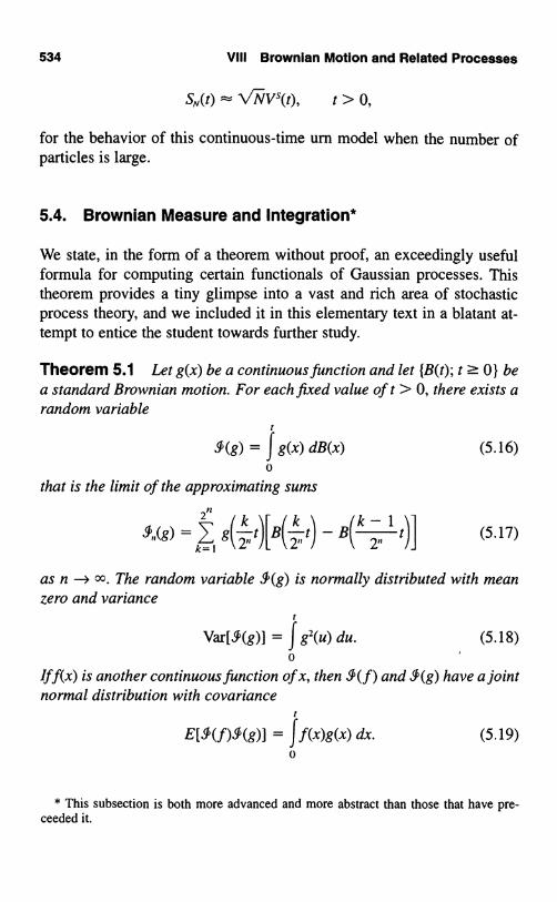
534 VIII Brownian Motion and Related Processes
SN,(t) ~ \/NVs(t), t > 0,
for the behavior of this continuous-time urn model when the number ofparticles is large.
5.4. Brownian Measure and Integration*
We state, in the form of a theorem without proof, an exceedingly usefulformula for computing certain functionals of Gaussian processes. Thistheorem provides a tiny glimpse into a vast and rich area of stochasticprocess theory, and we included it in this elementary text in a blatant at-tempt to entice the student towards further study.
Theorem 5.1 Let g(x) be a continuous function and let {B(t); t ? 0} bea standard Brownian motion. For each fixed value oft > 0, there exists arandom variable
t
(g) = f g(x) dB(x) (5.16)0
that is the limit of the approximating sums
211
)J = (B k
15.(g) I g " t
(t)]
"t) - ,B(
( .17)2k-1
2L 2
as n - oo. The random variable J(g) is normally distributed with meanzero and variance
t
Var[J(g)] = Jg2(u) du. (5.18)0
Iff(x) is another continuous function of x, then J (f) and ,9(g) have a jointnormal distribution with covariance
t
E[,9(f).(g)] = Jf(x)g(x) dx. (5.19)0
* This subsection is both more advanced and more abstract than those that have pre-ceeded it.

S. The Ornstein-Uhlenbeck Process 535
The proof of the theorem is more tedious than difficult, but it does requireknowledge of facts that are not included among our prerequisites. The the-orem asserts that a sequence of random variables, the Riemann approxi-mations, converge to another random variable. The usual proof beginswith showing that the expected mean square of the difference betweendistinct Riemann approximations satisfies the Cauchy criterion for con-vergence, and then goes on from there.
When g(x) is differentiable, then an integration by parts may be vali-dated, which shows that
t t
J g(x) dB(x) = g(t)B(t) - J B(x)g'(x) dx, (5.20)0 0
and this approach may yield a concrete representation of the integral incertain circumstances. For example, if g(x) = 1, then g'(x) = 0, and
t
Ji dB(x) = g(t)B(t) - 0 = B(t),0
as one would hope. When g(x) = t - x, then g'(x) _ -1, andt t
J(t_x)dB(x)__JB(x)dx. (5.21)0 0
The process on the right side of (5.21) is called integrated Brownian mo-tion. Theorem 5.1 then asserts that integrated Brownian motion is nor-mally distributed with mean zero and variance
Var[ J B(x) dx] = J (t - x)2 dx =t3
.
0 0
The calculus of the Brownian integral of Theorem 5.1 offers a fresh andconvenient way to determine functionals of some Gaussian processes. Forexample, in the case of the Ornstein-Uhlenbeck process, we have the in-tegral representation
t
V(t) = ve-9' + o- J e-g"-"' dB(u). (5.22)
The second term on the right of (5.22) expresses the random componentof the Ornstein-Uhlenbeck process as an exponentially weighted moving

536 VIII Brownian Motion and Related Processes
average of infinitesimal Brownian increments. According to Theorem 5.1,this random component has mean zero and is normally distributed. We useTheorem 5.1 to determine the covariance. For 0 < s < t,
Cov[V(s), V(t)] = E({V(s) - ve-1) {V(t) - ve-a'}]
= 0-2EI f e-a(S-14) dB(u) f dB(w)10 0 J
I
= o-2 f 1(u < du0
= o'ze-a(s+t) f eza" du
0
in agreement with (5.5).
0, 2 ' _ 1)e(e)2
2
Example The Position Process Revisited Let us assume that V(0) =v = 0. The integral of the Ornstein-Uhlenbeck velocity process gives theparticle's position S(t) at time t. If we replace the integrand by its repre-sentation (5.22) (v = 0), we obtain
t r s
S(t) = f V(s) ds = o- f f e-a(S-"' dB(u) ds0 00
I t
o- f f e-a(s-") ds dB(u)0 ut t
o- f ea" f e-R` ds dB(u) (5.23)o It
to- eau(e-a' - e-a') dB(u)
0
I
_ 0' f (I - e-a('-')) dB(u).go

S. The Ornstein-Uhlenbeck Process 537
Theorem 5.1 applied to (5.23) tells us that the position S(t) at time t is nor-mally distributed with mean zero and variance
Var[S(t)] = 02 f [I - e-jS(`-" )]2 du0
t
_ 0' f (1 - e-s"')2dw
F3' o
2
911 t - (1 - e ') + 2f3(1 _ e-,sr)]
in agreement with (5.9). Problem 5.4 calls for using Theorem 5.1 to de-termine the covariance between the velocity V(t) and position S(t).
The position process under an Ornstein-Uhlenbeck velocity behaveslike a Brownian motion over large time spans, and we can see this moreclearly from the Brownian integral representation in (5.23). If we carryout the first term in the integral (5.23) and recognize that the second partis V(t) itself, we see that
r
S(t) _ 0, f (1 - e-P('-'4) dB(u)0
air-u)ldB(u)Q[B(t) - f e ]
0
1=
R[UB(t) - V(t)].
(5.24)
Let us introduce a rescaled position process that will allow us to better seechanges in position over large time spans. Accordingly, for N > 0, let
1
SN(t) = -S(Nt)
(5.25)
_ , [O-J§(t) + ,V(t)],
538 VIII Brownian Motion and Related Processes
wherea(t) = B(Nt)/\/N remains a standard Brownian motion. (See Exer-cise 1.2.) Because the variance of V(t) is always less than or equal to0.21(2/3), the variance of V(t)/HIV becomes neglible for large N. Equation(5.25) then shows more clearly in what manner the position process be-comes like a Brownian motion: For large N,
o,S\,(t)
aB(t).
Exercises
5.1. An Ornstein-Uhlenbeck process V(t) has 0-2 = 1 and /3 = 0.2. Whatis the probability that V(t) <_ 1 for t = 1, 10, and 100? Assume thatV(0) = 0.
5.2. The velocity of a certain particle follows an Ornstein-Uhlenbeckprocess with .2 = 1 and /3 = 0.2. The particle starts at rest (v = 0) fromposition S(0) = 0. What is the probability that it is more than one unitaway from its origin at time t = 1. What is the probability at times t = 10and t = 100?
5.3. Let ,, 62, ... be independent standard normal random variablesand /3 a constant, 0 < /3 < 1. A discrete analogue to the Ornstein-Uhlenbeck process may be constructed by setting
Vo=v and for n?1.(a) Determine the mean value function and covariance function for
(b) Let AV = V,,. Determine the conditional mean and varianceof AV, given that V = v.
Problems
5.1. Let e,, e,, ... be independent standard normal random variablesand /3 a constant, 0 < /3 < 1. A discrete analogue to the Ornstein-Uhlenbeck process may be constructed by setting
V. = v and V = (1 - 6,, for n ? 1.

Problems 539
(a) Show that
Vr = (1 - N)"v + , (1 - 3)n _k6k-
k=1N/
Comment on the comparison with (5.22).(b) Let AV,, = V - S = v + V, + + V,,, and B,,
6, + + , Show that
B
Compare and contrast with (5.24).
5.2. Let _S(t) be the position process corresponding to an Ornstein-Uhlenbeck velocity V(t). Assume that S(0) = V(0) = 0. Obtain the co-variance between S(t) and V(t).
5.3. Verify the option valuation formulation (5.10).
Hint: Use the result of Exercise 4.6.
5.4. In the Ehrenfest urn model (see III, Section 3.2) for molecular dif-fusion through a membrane, if there are i particles in urn A, the probabil-ity that there will be i + 1 after one time unit is 1 - i/(2N), and the prob-ability of i - 1 is i/(2N), where 2N is the aggregate number of particles inboth urns. Following III, Section 3.2, let Y be the number of particles inurn A after the nth transition, and let X,, = Y - N. Let OX = X,, bethe change in urn composition. The probability law is
We anticipate a limiting process in which the time between transitions be-comes small and the number of particles becomes large. Accordingly, letAt = 1/N and measure fluctuations of a rescaled process in units of order1/N/"N-. The definition of the rescaled process is
VN(t) =XjNj
Note that in the duration t = 0 to t = 1 in the rescaled process, thereare N transitions in the urns, and a unit change in the rescaled process

540 VIII Brownian Motion and Related Processes
corresponds to a fluctuation of order 1l'"N- in the urn composition. LetAV = VN(t + 1/N) - VN(t) be the displacement in the rescaled processover the time interval At = 1/N. Show that
E[OV IVN(t) = v] _\ 2 2V / V"N(2 + 2\/N)
-v(N) = VAt,
and that (AV)2 = 1/N, whence
Var[AVIVN(t) = v] = E[(OV)Z] - {E[OV])2
= N + o(N) = At + o(Ot).

Chapter IXQueueing Systems
1. Queueing Processes
A queueing system consists of "customers" arriving at random times tosome facility where they receive service of some kind and then depart. Weuse "customer" as a generic term. It may refer, for example, to bona fidecustomers demanding service at a counter, to ships entering a port, tobatches of data flowing into a computer subsystem, to broken machinesawaiting repair, and so on. Queueing systems are classified according to
1. The input process, the probability distribution of the pattern of ar-rivals of customers in time;
2. The service distribution, the probability distribution of the randomtime to serve a customer (or group of customers in the case of batchservice); and
3. The queue discipline, the number of servers and the order of cus-tomer service.
While a variety of input processes may arise in practice, two simple andfrequently occurring types are mathematically tractable and give insightsinto more complex cases. First is the scheduled input, where customers ar-rive at fixed times T, 2T, 3T, .... The second most common model is the"completely random" arrival process, where the times of customer ar-rivals form a Poisson process. Understanding the axiomatic developmentof the Poisson process in V may help one to evaluate the validity of the

542 IX Queueing Systems
Poisson assumption in any given application. Many theoretical results areavailable when the times of customer arrivals form a renewal process. Ex-ponentially distributed interarrival times then correspond to a Poissonprocess of arrivals as a special case.
We will always assume that the durations of service for individual cus-tomers are independent and identically distributed nonnegative randomvariables and are independent of the arrival process. The situation in whichall service times are the same fixed duration D, is, then, a special case.
The most common queue discipline is first come, first served, wherecustomers are served in the same order in which they arrive. All of themodels that we consider in this chapter are of this type.
Queueing models aid the design process by predicting system perfor-mance. For example, a queueing model might be used to evaluate thecosts and benefits of adding a server to an existing system. The models en-able us to calculate system performance measures in terms of more basicquantities. Some important measures of system behavior are
1. The probability distribution of the number of customers in the sys-tem. Not only do customers in the system often incur costs, but inmany systems, physical space for waiting customers must beplanned for and provided. Large numbers of waiting customers canalso adversely affect the input process by turning potential new cus-tomers away. (See Section 4.1 on queueing with balking.)
2. The utilization of the server(s). Idle servers may incur costs withoutcontributing to system performance.
3. System throughput. The long run number of customers passingthrough the system is a direct measure of system performance.
4. Customer waiting time. Long waits for service are annoying in thesimplest queueing situations and directly associated with major costsin many large systems such as those describing ships waiting tounload at a port facility or patients awaiting emergency care at ahospital.
1.1. The Queueing Formula L = A W
Consider a queueing system that has been operating sufficiently long tohave reached an appropriate steady state, or a position of statistical equi-librium. Let

1. Queueing Processes 543
L = the average number of customers in the system;A = the rate of arrival of customers to the system; and
W = the average time spent by a customer in the system.
The equation L = AW is valid under great generality for such systems andis of basic importance in the theory of queues, since it directly relates twoof our most important measures of system performance, the mean queuesize and the mean customer waiting time in the steady state, that is, meanqueue size and mean customer waiting time evaluated with respect to alimiting or stationary distribution for the process.
The validity of L = A W does not rest on the details of any particularmodel, but depends only upon long run mass flow balance relations. Tosketch this reasoning, consider a time T sufficiently long so that statisticalfluctuations have averaged out. Then the total number of customers tohave entered the system is AT, the total number to have departed is A(T -W), and the net number remaining in the system L must be the difference
L= AT - [A(T- W)] = AW.
Figure 1.1 depicts the relation L = AW.Of course, what we have done is by no means a proof, and indeed, we
shall give no proof. We shall, however, provide several sample verifi-cations of L = A W where L is the mean of the stationary distribution of
time(a) Random arrivals, departures (b) Smoothed values
Figure 1.1 The cumulative number of arrivals and departures in a queueingsystem. The smoothed values in (b) are meant to symbolize longrun averages. The rate of arrivals per unit time is A, the meannumber in the system is L, and the mean time a customer spendsin the system is W.

544 IX Queueing Systems
customers in the system, W is the mean customer time in the system de-termined from the stationary distribution, and A is the arrival rate in aPoisson arrival process.
Let Lo be the average number of customers waiting in the system whoare not yet being served, and let Wo be the average waiting time in the sys-tem excluding service time. In parallel to L = AW, we have the formula
Lo = AW0 (1.1)
The total waiting time in the system is the sum of the waiting time beforeservice and the service time. In terms of means, we have
W = Wo + mean service time. (1.2)
1.2. A Sampling of Queueing Models
In the remainder of this chapter we will study a variety of queueing sys-tems. A standard shorthand is used in much of the queueing literature foridentifying simple queueing models. The shorthand assumes that the ar-rival times form a renewal process, and the format A/B/c uses A to de-scribe the interarrival distribution, B to specify the individual customerservice time distribution, and c to indicate the number of servers. Thecommon cases for the first two positions are G = GI for a general or ar-bitrary distribution, M (memoryless) for the exponential distribution, Ek(Erlang) for the gamma distribution of order k, and D for a deterministicdistribution, a schedule of arrivals or fixed service times.
Some examples discussed in the sequel are the following:
The M/M/1 queue Arrivals follow a Poisson process; service timesare exponentially distributed; and there is a single server. The numberX(t) of customers in the system at time t forms a birth and deathprocess. (See Section 2.)
The M/M/oo queue There are Poisson arrivals and exponentially dis-tributed service times. Any number of customers are processed simul-taneously and independently. Often self-service situations may be de-scribed by this model. In the older literature this was called the"telephone trunking problem."

1. Queueing Processes 545
The MIG11 queue In this model there are Poisson arrivals but arbi-trarily distributed service times. The analysis proceeds with the help ofan embedded Markov chain.
More elaborate variations will also be set forth. Balking is the refusalof new customers to enter the system if the waiting line is too long. Moregenerally, in a queueing system with balking, an arriving customer entersthe system with a probability that depends on the size of the queue. Hereit is important to distinguish between the arrival process and the inputprocess, as shown in Figure 1.2. A special case is a queue with overflow,in which an arriving customer enters the queue if and only if there is atleast one server free to begin service immediately.
In a priority queue, customers are allowed to be of different types. Boththe service discipline and the service time distribution may vary with thecustomer type.
A queueing network is a collection of service facilities where the de-partures from some stations form the arrivals of others. The network isclosed if the total number of customers is fixed, these customers continu-ously circulating through the system. The machine repair model (see theexample entitled "Repairman Models" in VI, Section 4) is an example ofa closed queueing network. In an open queueing network, customers mayarrive from, and depart to, places outside the network, as well as movefrom station to station. Queueing network models have found much recentapplication in the design of complex information processing systems.
Departssystemwith
probability1 -Pn
Waitingline
X XXXX
0 Enters system n customersArrival with probability Input waiting
process pn process
Servicefacility
Figure 1.2 If n customers are waiting in a queueing system with balking, anarriving customer enters the system with probability pn and doesnot enter with probability 1 - p,.

546 IX Queueing Systems
Exercises
1.1. What design questions might be answered by modeling the follow-ing queueing systems?
The Customer The Server(a) Arriving airplanes The runway(b) Cars A parking lot(c) Broken TVs Repairman(d) Patients Doctor(e) Fires Fire engine company
What might be reasonable assumptions concerning the arrival process,service distribution, and priority in these instances?
1.2. Consider a system, such as a barber shop, where the service re-quired is essentially identical for each customer. Then actual service timeswould tend to cluster near the mean service time. Argue that the expo-nential distribution would not be appropriate in this case. For what typesof service situations might the exponential distribution be quite plausible?
1.3. Oil tankers arrive at an offloading facility according to a Poissonprocess whose rate is A = 2 ships per day. Daily records show that thereis an average of 3 ships unloading or waiting to unload at any instant intime. On average, what is the duration of time that a ship spends in port?Assume that a ship departs immediately after unloading.
Problems
1.1. Two dump trucks cycle between a gravel loader and a gravel un-loader. Suppose that the travel times are insignificant relative to the loadand unload times, which are exponentially distributed with parameters µand A, respectively. Model the system as a closed queueing network. De-termine the long run gravel loads moved per unit time.
Hint: Refer to the example entitled "Repairman Models" in Section4ofVI.

2. Poisson Arrivals, Exponential Service Times 547
2. Poisson Arrivals, Exponential Service Times
The simplest and most extensively studied queueing models are thosehaving a Poisson arrival process and exponentially distributed servicetimes. In this case the queue size forms a birth and death process (see Sec-tions 3 and 4 of VI), and the corresponding stationary distribution is read-ily found.
We let A denote the intensity, or rate, of the Poisson arrival process andassume that the service time distribution is exponential with parameter A.The corresponding density function is
g(x) = Ae-- for x > 0. (2.1)
For the Poisson arrival process we have
Pr{An arrival in [t, t + h)} = Ah + o(h) (2.2)
and
Pr{No arrivals in [t, t + h) } = 1 - Ah + o(h). (2.3)
Similarly, the memoryless property of the exponential distribution as ex-pressed by its constant hazard rate (see I, Section 4.2) implies that
Pr(A service is completed in [t, t + h)IService in progress at time t}
= Ah + o(h), (2.4)
and
Pr{Service not completed in [t, t + h)IService in progress at time t}
= 1 - µh + o(h). (2.5)
The service rate p applies to a particular server. If k servers are simulta-neously operating, the probability that one of them completes service in atime interval of duration h is (kµ)h + o(h), so that the system service rateis kµ. The principle used here is the same as that used in deriving the in-finitesimal parameters of the Yule process (VI, Section 1).
We let X(t) denote the number of customers in the system at time t,counting the customers undergoing service as well as those awaiting ser-vice. The independence of arrivals in disjoint time intervals together withthe memoryless property of the exponential service time distribution

548 IX Queueing Systems
implies that X(t) is a time homogeneous Markov chain, in particular, abirth and death process. (See Sections 3 and 4 of VI.)
2.1. The MIM/1 System
We consider first the case of a single server and let X(t) denote the num-ber of customers in the system at time t. An increase in X(t) by one unitcorresponds to a customer arrival, and in view of (2.2) and (2.5) and thepostulated independence of service times and the arrival process, we have
Pr{X(t + h) = k + 1IX(t) = k) = [Ah + o(h)] X [1 - µh + o(h)]
= Ah + o(h) for k = 0, 1, ... .
Similarly, a decrease in X(t) by one unit corresponds to a completion ofservice, whence
Pr{X(t+h)=k- lIX(t)=k} =µh+o(h) fork= 1,2.....Then X(t) is a birth and death process with birth parameters
Ak - A fork=0,1,2,...and death parameters
Ak=1h fork= 1,2.....Of course, no completion of service is possible when the queue is empty.We thus specify µ0 = 0.
Let
I r k = lim Pr{X(t) = k} for k = 0, 1, .. .
be the limiting, or equilibrium, distribution of queue length. Section 4 ofVI describes a straightforward procedure for determining the limiting dis-tribution lTk from the birth and death parameters Ak and µk. The techniqueis to first obtain intermediate quantities 8; defined by
00 = 1 and 0; =AOA, A,_,
for j ? 1, (2.6)

2. Poisson Arrivals, Exponential Service Times 549
and then
?r0 =o
el and irk = 0kir0 =Y"'=
o el fork 1, 1. (2.7)
When 1 o 0, _ 00, then lim,.x Pr{X(t) = k) = 0 for all k, and the queuelength grows unboundedly in time.
For the M/M/1 queue at hand we readily compute 00 = 1 and 8; = (A/µyfor j = 1, 2, .... Then
j=o
= 00 ifA?µ.Thus, no equilibrium distribution exists when the arrival rate A is equal toor greater than the service rate A. In this case the queue length grows with-out bound.
When A < µ, a bona fide limiting distribution exists, given by
1 A7r0 =f0 =I --Ii-
and
7Fk= 1'00k=1 -A )(- A
) fork=0, 1,IL µ
(2.8)
(2.9)
The equilibrium distribution (2.9) gives us the answer to many questionsinvolving the limiting behavior of the system. We recognize the form of(2.9) as that of a geometric distribution, and then reference to I, Section3.3 gives us the mean queue length in equilibrium to be
L=A
µ - A
The ratio p = A/µ is called the traffic intensity,
arrival rate AP = =system service rate µ
1
x1 ifA<
J=O A) (I A//J,)
(2.10)
(2.11)

550 IX Queueing Systems
As the traffic intensity approaches one, the mean queue lengthL = p/(1 - p) becomes infinite. Again using (2.8), the probability of beingserved immediately upon arrival is
Iro = 1 - -,µ
the probability, in the long run, of finding the server idle. The serverutilization, or long run fraction of time that the server is busy, is1 - iro = A/µ.
We can also calculate the distribution of waiting time in the stationarycase when k < µ. If an arriving customer finds n people in front of him,his total waiting time T, including his own service time, is the sum of theservice times of himself and those ahead, all distributed exponentiallywith parameter µ, and since the service times are independent of thequeue size, T has a gamma distribution of order n + 1 with scale parame-ter µ,
r +iT,ne-kTPr{T ahead} = f µI'(n + 1) dT. (2.12)
By the law of total probability, we have
Pr{T :5 t} Pr(T t1n ahead) X (A (1 -n=o
since (A/µ)"(1 - A/µ) is the probability that in the stationary case a cus-tomer on arrival will find n ahead in line. Now, substituting from (2.12),we obtain
Pr{T s t} =x r n+1 -µT nµ Tne
(p.)(A1- A)dTr(n + 1) µ/
=r
µe-µT(1 -0
),L dTr(n + 1)
A A= J (1 - µ)µ expj-Tµ(1 - µ)} dT = 1 - exp[-t(µ - A)],
which is also an exponential distribution.
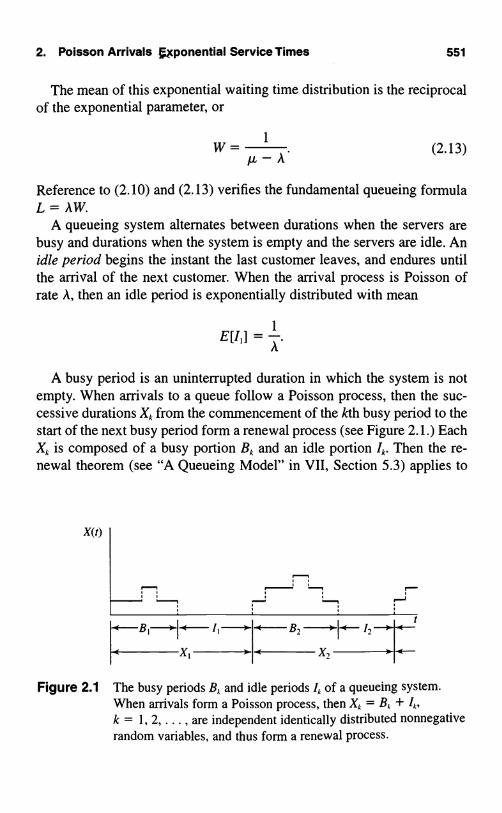
2. Poisson Arrivals cponential Service Times 551
The mean of this exponential waiting time distribution is the reciprocalof the exponential parameter, or
W= 1
(2.13)µ - A
Reference to (2.10) and (2.13) verifies the fundamental queueing formulaL = A.W.
A queueing system alternates between durations when the servers arebusy and durations when the system is empty and the servers are idle. Anidle period begins the instant the last customer leaves, and endures untilthe arrival of the next customer. When the arrival process is Poisson ofrate A, then an idle period is exponentially distributed with mean
A busy period is an uninterrupted duration in which the system is notempty. When arrivals to a queue follow a Poisson process, then the suc-cessive durations Xk from the commencement of the kth busy period to thestart of the next busy period form a renewal process (see Figure 2.1.) EachXk is composed of a busy portion Bk and an idle portion Ik. Then the re-newal theorem (see "A Queueing Model" in VII, Section 5.3) applies to
X(t)
HcB,< /i>IE -XI 0
< B, 0F 1, r---X,
Figure 2.1 The busy periods Bk and idle periods 1k of a queueing system.When arrivals form a Poisson process, then Xk = Bk + Ik,k = 1, 2, ... , are independent identically distributed nonnegativerandom variables, and thus form a renewal process.

552 IX Queueing Systems
tell us that po(t), the probability that the system is empty at time t, con-verges to
lim po(t) = lro =E[II l
E[I,] + E[B,]
We substitute the known quantities ir,, = 1 - Alµ and E[I,] = 1/A toobtain
1 1/A + E[B,]'
which gives
1E[B,] _
A
for the mean length of a busy period.In Section 3, in studying the M/G/1 system we will reverse this reason-
ing, calculate the mean busy period directly, and then use renewal theoryto determine the server idle fraction Tro.
2.2 The M/M/cc System
When an unlimited number of servers are always available, then all cus-tomers in the system at any instant are simultaneously being served. Thedeparture rate of a single customer being µ, the departure rate of k cus-tomers is kµ, and we obtain the birth and death parameters
Ak = A and µk = kµ for k = 0, 1. ... .The auxiliary quantities of (2.6) are
AOA, ... Ak-I 1 A kek= =k(µ) fork=0,1,...,
µiµ2 µk
which sum to
= e"''`

2. Poisson Arrivals, Exponential Service Times 553
whence
1-NµaT0 = Ik0ek=C
and
(Aµ)ke-uµ
ark= Okaro=k!
fork= 0, 1,..., (2.14)
a Poisson distribution with mean queue length
Since a customer in this system begins service immediately upon ar-rival, customer waiting time consists only of the exponentially distributedservice time, and the mean waiting time is W = 1/p.. Again, the basicqueueing formula L = A W is verified.
The M/G/cG queue will be developed extensively in the next section.
2.3. The MMIs System
When a fixed number s of servers are available and the assumption ismade that a server is never idle if customers are waiting, then the appro-priate birth and death parameters are
Ak=A fork= 1,2,...,
µk -Jkµ fork=0,sµ fork > s.
If X(t) is the number of customers in the system at time t, then the num-ber undergoing service is min(X(t), s), and the number waiting for serviceis max{X(t) - s, 0}. The system is depicted in Figure 2.2.
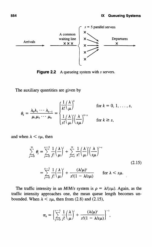
554 IX Queueing Systems
Arrivals
A commonwaiting line X Departures
X X X X X
X 7X/
Figure 2.2 A queueing system with s servers.
The auxiliary quantities are given by
ek-AoAI...Ak_I
and when A < sµ, then
S! tL Sjtk)
fork=0,1,...,s,
for k ? s,
(-l + z ,(
)'(z S! /-t SAj=0 j=0 j! A j=S
(2.15)
' 1 (A 1' + (Alto for A < sµJ s!(1 - A/sr=c j! N N-)
The traffic intensity in an MIMIs system is p = Al(sli). Again, as thetraffic intensity approaches one, the mean queue length becomes un-bounded. When A < sµ, then from (2.8) and (2.15),
s = 5 parallel servers
X
,To
= (A )i
Ij'=() s!(1 - Alsµ)1j! A +

Exercises
and
555
1 A kki(µ)ITO
s k
fork=0,1,...,s,(2.16)
IT0s! \ul (su) fork? s,
We evaluate L0, the mean number of customers in the system waiting for,and not undergoing, service. Then
Lo=7, (J-s)lrj=7' kir,j=s k=0
k=0 YJAIAS kµlk
= so(µ).,7,
k( k
7ro A ls (A/sµ)
= s! (µl (1 - Alsp)2'
Then
W = W0 +
and
Exercises
L=AW=A(W0+ 1 I=LO+ Aµ/ µ
k
(2.17)
2.1. Customers arrive at a tool crib according to a Poisson process ofrate A = 5 per hour. There is a single tool crib employee, and the individ-ual service times are exponentially distributed with a mean service time of

556 IX Queueing Systems
10 minutes. In the long run, what is the probability that two or more work-ers are at the tool crib being served or waiting to be served?
2.2. On a single graph, plot the server utilization 1 - Tro = p and themean queue length L = p/(1 - p) for the M/M/l queue as a function ofthe traffic intensity p = A/µ for 0 < p < 1.
2.3. Customers arrive at a checkout station in a market according to aPoisson process of rate A = 1 customer per minute. The checkout stationcan be operated with or without a bagger. The checkout times for cus-tomers are exponentially distributed, and with a bagger the mean check-out time is 30 seconds, while without a bagger this mean time increases to50 seconds. Compare the mean queue lengths with and without a bagger.
Problems
2.1. Determine explicit expressions for 7r0 and L for the MIMIs queuewhen s = 2. Plot I - iro and L as a function of the traffic intensityp = A/2µ.
2.2. Determine the mean waiting time W for an M/M12 system whenA = 2 and µ = 1.2. Compare this with the mean waiting time in an M/M11system whose arrival rate is A = 1 and service rate is µ = 1.2. Why is therea difference when the arrival rate per server is the same in both cases?
2.3. Determine the stationary distribution for an MIM12 system as afunction of the traffic intensity p = A/2µ, and verify that L = AW.
2.4. The problem is to model a queueing system having finite capacity.We assume arrivals according to a Poisson process of rate A, independentexponentially distributed service times having mean 1/µ, a single server,and a finite system capacity N. By this we mean that if an arriving cus-tomer finds that there are already N customers in the system, then that cus-tomer does not enter the system and is lost.
Let X(t) be the number of customers in the system at time t. Supposethat N = 3 (2 waiting, 1 being served).
(a) Specify the birth and death parameters for X(t).(b) In the long run, what fraction of time is the system idle?(c) In the long run, what fraction of customers are lost?

Problems 557
2.5. Customers arrive at a service facility according to a Poissonprocess having rate A. There is a single server, whose service times are ex-ponentially distributed with parameter µ. Let N(t) be the number of peo-ple in the system at time t. Then N(t) is a birth and death process withparameters A = A for n ? 0 and µ = µ for n ? 1. Assume A < A. Thenlrk = (1 - A/p)(Alµ)k, k ? 0, is a stationary distribution for N(t); cf. equa-tion (2.9).
Suppose the process begins according to the stationary distribution.That is, suppose Pr{N(0) = k} _ ffk for k = 0, 1, .... Let D(t) be thenumber of people completing service up to time t. Show that D(t) has aPoisson distribution with mean At.
Hint: Let Pk;(t) = Pr{D(t) = jIN(0) = k} and P(t) _ I 1rkPk;(t) =Pr{D(t) = j}. Use a first step analysis to show that P0;(t + At) =A(Ot)P,;(t) + [1 - A(Ot)]Po;(t) + o(Ot), and for k = 1, 2, ... ,
Pk;(t + At) = µ(Ot)Pk ,.;-I(t) +
[1 - (A + µ)(Ot)]PkJ(t) + 0(t).
Then use P;(t) _ Ik irrPk;(t) to establish a differential equation. Use the ex-plicit form of Irk given in the problem.
2.6. Customers arrive at a service facility according to a Poissonprocess of rate A. There is a single server, whose service times are expo-nentially distributed with parameter µ. Suppose that "gridlock" occurswhenever the total number of customers in the system exceeds a capacityC. What is the smallest capacity C that will keep the probability of grid-lock, under the limiting distributing of queue length, below 0.001? Ex-press your answer in terms of the traffic intensity p = A/µ.
2.7. Let X(t) be the number of customers in an M/MIcc queueing systemat time t. Suppose that X(0) = 0.
(a) Derive the forward equations that are appropriate for this processby substituting the birth and death parameters into VI, (3.8).
(b) Show that M(t) = E[X(t)] satisfies the differential equationM'(t) = A - AM(t) by multiplying the jth forward equation by jand summing.
(c) Solve for M(t).

558 IX Queueing Systems
3. General Service Time Distributions
We continue to assume that the arrivals follow a Poisson process of rateA. The successive customer service times Y,, Y2, ... , however, are now al-lowed to follow an arbitrary distribution G(y) = Pr{ Yk y } having a fi-nite mean service time v = E[1 ]. The long run service rate is µ = 1/v.Deterministic service times of an equal fixed duration are an importantspecial case.
3.1. The MIGI1 System
If arrivals to a queue follow a Poisson process, then the successive dura-tions Xk from the commencement of the kth busy period to the start of thenext busy period form a renewal process. (A busy period is an uninter-rupted duration when the queue is not empty. See Figure 2.1.) Each Xk iscomposed of a busy portion Bk and an idle portion Ik. Then po(t), the prob-ability that the system is empty at time t, converges to
lim po(t) = pro =E[I l]
E[XI](3.1)
E[11]
E[111 + E[B, ]
by the renewal theorem (see "A Queueing Model" in VII, Section 5.3).The idle time is the duration from the completion of a service that emp-
ties the queue to the instant of the next arrival. Because of the memory-less property that characterizes the interarrival times in a Poisson process,each idle time is exponentially distributed with mean E[l,] = 1/A.
The busy period is composed of the first service time Y,, plus busy pe-riods generated by all customers who arrive during this first service time.Let A denote this random number of new arrivals. We will evaluate theconditional mean busy period given that A = n and Y, = y. First,
E[BJA = 0, Y, = y] = y,
because when no customers arrive, the busy period is composed of the

3. General Service Time Distributions- 559
first customer's service time alone. Next, consider the case in whichA = 1, and let B' be the duration from the beginning of this customer'sservice to the next instant that the queue is empty. Then
E[B, I A = 1, Y, = y] = y + E[B']
= y + E[B, ],
because upon the completion of service for the initial customer, the singlearrival begins a busy period B' that is statistically identical to the first, sothat E[B'] = E[B,]. Continuing in this manner we deduce that
E[B,I A = n, Y, = y] = y + nE[B,]
and then, using the law of total probability, thatx
E[B,IY, = y] = 7, E[B,IA = n, Y, = y] Pr{A = nIY, = y)n=0
v + nE[B 11(Ay)'e'
v
n=0 n.
= y+ 1lyE[B,].
Finally,
E[BI] = J E[B,I Y, = y] dG(y)0
X
= J {y + AyE[B,] } dG(y)0
= v{ 1 + AE[B,] }.
Since E[B,] appears on both sides of (3.2), we may solve to obtain
E[B,] = 1
v_ Av, provided that Av < 1.
(3.2)
(3.3)
To compute the long run fraction of idle time, we use (3.3) and

560 IX Queueing Systems
E[I1l
E[lll + E[B,l
1/A
1/A + v/(1 - AV)(3.4)
=1-Av ifAv<1.Note that (3.4) agrees, as it must, with the corresponding expression
(2.8) obtained for the M/M11 queue where v = 1/µ. For example, ifarrivals occur at the rate of A = 2 per hour and the mean service time is20 minutes, or v = ; hours, then in the long run the server is idle1 - 2(3) _ ; of the time.
The Embedded Markov Chain
The number X(t) of customers in the system at time t is not a Markovprocess for a general M/GI1 system, because if one is to predict the futurebehavior of the system, one must know, in addition, the time expended inservice for the customer currently in service. (It is the memoryless prop-erty of the exponential service time distribution that makes this additionalinformation unnecessary in the M/M/1 case.)
Let X,,, however, denote the number of customers in the system imme-diately after the departure of the nth customer. Then {X } is a Markovchain. Indeed, we can write
1 + A if X,,-, > 0,
X"= All if 0, (3.5)
_(X,,-,-1)++ A,where A,, is the number of customers that arrive during the service of thenth customer and where x+ = max( x, 0). Since the arrival process is Pois-son, the number of customers A,, that arrive during the service of the nthcustomer is independent of earlier arrivals, and the Markov property fol-lows instantly. We calculate
f Pr{A,,0
_ ( (Ay)ke-z,.
J dG(y),0 k!
(3.6)

3. General Service Time Distributions 561
and then, for j = 0, 1, ... ,
P;=Pr{X,, =i} 1)+}
a;_;+, for i ? 1, j ? i + 1, (3.7)
a; for i = 0.
The Mean Queue Length in Equilibrium L
The embedded Markov chain is of special interest in the M/G/1 queue be-cause in this particular instance, the stationary distribution fir) for theMarkov chain {X } equals the limiting distribution for the queue lengthprocess {X(t)}. That is, lim, Pr{X(t) = j) = Pr{X = j}. We willuse this helpful fact to evaluate the mean queue length L.
The equivalence between the stationary distribution for the Markovchain and that for the non-Markov process {X(t) } is rather subtle. Itis not the consequence of a general principle and should not be assumedto hold in other circumstances without careful justification. The equiva-lence in the case at hand is sketched in an appendix to this section.
We will calculate the expected queue length in equilibriumL = lim, E[X(t)] by calculating the corresponding quantity in the em-bedded Markov chain, L = lim, ,,. E[X ]. If X = X,, is the number of cus-tomers in the system after a customer departs and X' is the number afterthe next departure, then in accordance with (3.5),
X'=X-S+N, (3.8)
where N is the number of arrivals during the service period and
I1 ifX> 0,0 ifX=0.
In equilibrium, X has the same distribution as does X', and in particular,
L = E[X] = E[X'], (3.9)
and taking expectation in (3.8) gives
E[X'] = E[X] - E[S] + E[N],
and, by (3.9) and (3.4), then
E[N] = E[S] = 1 - iro = Av. (3.10)

562 IX Queueing Systems
Squaring (3.8) gives
(X')22=X22+52 +N2-26X+2N(X- 6),
and since 6 = 6 and X6 = X, then
(X')2 = X2 + S + N2 - 2X + 2N(X - 6). (3.11)
Now N, the number of customers that arrive during a service period, is in-dependent of X, and hence of 6, so that
E[N(X - 6)] = E[N]E[X - 6], (3.12)
and because X and X' have the same distribution, then
E[(X')2] = E[X2]. (3.13)
Taking expectations in (3.11) we deduce that
E[(X')2] = E[X2] + E[6] + E[N22] - 2E[X] + 2E[N]E[X - 6],
and then substituting from (3.10) and (3.13), we obtain
0 = Av + E[N2] - 2L + 2Av(L - Av),
or
AP + E[N22] - 2(A V)2L 2(1-Av) (3.14)
It remains to evaluate E[N22], where N is the number of arrivals duringa service time Y. Conditioned on Y = y, the random variable N has a Pois-son distribution with a mean (and variance) equal to Ay [see (3.6)],whence E[N2I Y = y] = Ay + (Ay)2. Using the law of total probability thengives
[E[NIYE[N2] = = y] dG(y)0
X
= A J y dG(y) + A2 f y2 dG(y) (3.15)0 0
= AY + A2 (.T2 + u2),

3. General Service Time Distributions 563
where TZ is the variance of the service time distribution G(y). Substituting(3.15) into (3.14) gives
2Av + A2T2 - (AV)2L = 2(1 - Av)
A2T2 + p2
V 2(1-p)'
where p = Av is the traffic intensity.Finally, W = L/lt, which simplifies to
A(T2 + V2)W=v+2(1 - p)
(3.16)
(3.17)
The results (3.16) and (3.17) express somewhat surprising facts. Theysay that for a given average arrival rate A and mean service time v, we candecrease the expected queue size L and waiting time W by decreasing thevariance of service time. Clearly, the best possible case in this respect cor-responds to constant service times, for which T2 = 0.
Appendix
We sketch a proof of the equivalence between the limiting queue size dis-tribution and the limiting distribution for the embedded Markov chain inan M/G/1 model. First, beginning at t = 0 let -q denote those instants whenthe queue size X(t) increases by one (an arrival), and let denote those in-stants when X(t) decreases by one (a departure). Let Y = X(rl -) denotethe queue length immediately prior to an arrival and let X,, = X(6, +) de-note the queue length immediately after a departure. For any queue lengthi and any time t, the number of visits of Y,, to i up to time t differs fromthe number of visits of X,, to i by at most one unit. Therefore, in the longrun the average visits per unit time of Y,, to i must equal the average vis-its of X,, to i, which is ir,, the stationary distribution of the Markov chain
Thus we need only show that the limiting distribution of {X(O) is thesame as that of which is X(t) just prior to an arrival. But because thearrivals are Poisson, and arrivals in disjoint time intervals are indepen-dent, it must be that X(t) is independent of an arrival that occurs at time t.

564 IX Queueing Systems
It follows that {X(t)} and have the same limiting distribution, andtherefore {X(t) } and the embedded Markov chain {X } have the same lim-iting distribution.
3.2. The M/G/x System
Complete results are available when each customer begins service imme-diately upon arrival independently of other customers in the system. Suchsituations may arise when modeling customer self-service systems. LetW1, W2, ... be the successive arrival times of customers, and let V, V2, .. .be the corresponding service times. In this notation, the kth customer is inthe system at time t if and only if W, s t (the customer arrived prior to t)and W + V > t (the service extends beyond t).
The sequence of pairs (W,, V,), (W,, V2), ... forms a marked Poissonprocess (see V, Section 6.2), and we may use the corresponding theory toquickly obtain results in this model. Figure 3.1 illustrates the marked Pois-
V
4
i
0
x(Wk, Vk)
W, W, I W W,
Wkt
W6 W
Figure 3.1 For the M/G/o queue the number of customers in the system attime t corresponds to the number of pairs (W V,) for whichW, <_ t and W, + V, > t. In the sample illustrated here, the num-ber of customers in the system at time t is 3.

3. General Service Time Distributions 565
son process. Then X(t), the number of customers in the system at time t,is also the number of points (W, Vk) for which Wk < t and Wk + Vk > t.That is, it is the number of points (Wk, Vk) in the unbounded trapezoid de-scribed by
A,= {(w,v):O_w<_tand v>t-w}. (3.18)
According to V, Theorem 6.1, the number of points in A, follows a Pois-son distribution with mean
µ(A) = Jj. A(dw) dG(v)Ai
= A J I J dG(v)} dw0 t-wt
=A J[1 -G(t-w)]dw0
t
= A J [1 - G(x)] dx.0
In summary,
pk(t) = Pr{X(t) = k}
A(Ar)ke-," >
k!for k = 0, 1, ... ,
where µ(A) is given by (3.19). As t - oo, then
x
I i m µ(A) = A J [1 - G(x)] dx = Av,0
(3.19)
where v is the mean service time. Thus we obtain the limiting distribution
(Av)ke-aP
1Tk =k!
fork=0,1,....

566 IX Queueing Systems
Exercises
3.1. Suppose that the service distribution in a single server queue is ex-ponential with rate p.; i.e., G(v) = 1 - e-µY for v > 0. Substitute the meanand variance of this distribution into (3.16) and verify that the resultagrees with that derived for the M/M/1 system in (2.10).
3.2. Consider a single-server queueing system having Poisson arrivalsat rate A. Suppose that the service times have the gamma density
Laya- ' e - {1y
g(Y) I ^ r(a) for y >_ 0,
where a > 0 and µ > 0 are fixed parameters. The mean service time isa/µ and the variance is a/µZ. Determine the equilibrium mean queuelength L.
3.3. Customers arrive at a tool crib according to a Poisson process ofrate A = 5 per hour. There is a single tool crib employee, and the individ-ual service times are random with a mean service time of 10 minutes anda standard deviation of 4 minutes. In the long run, what is the mean num-ber of workers at the tool crib either being served or waiting to be served?
3.4. Customers arrive at a checkout station in a market according to aPoisson process of rate A = 1 customer per minute. The checkout stationcan be operated with or without a bagger. The checkout times for cus-tomers are random. With a bagger the mean checkout time is 30 seconds,while without a bagger this mean time increases to 50 seconds. In bothcases, the standard deviation of service time is 10 seconds. Compare themean queue lengths with and without a bagger.
3.5. Let X(t) be the number of customers in an M/G/co queueing systemat time t. Suppose that X(0) = 0. Evaluate M(t) = E[X(t)], and show thatit increases monotonically to its limiting value as t - -.
Problems
3.1. Let X(t) be the number of customers in an M/GIc queueing systemat time t, and let Y(t) be the number of customers who have entered the

4. Variations and Extensions 567
system and completed service by time t. Determine the joint distributionof X(t) and Y(t).
3.2. In operating a queueing system with Poisson arrivals at a rate ofA = I per unit time and a single server, you have a choice of server mech-anisms. Method A has a mean service time of v = 0.5 and a variance inservice time of r 2 = 0.2, while Method B has a mean service time ofv = 0.4 and a variance of r2 = 0.9. In terms of minimizing the waitingtime of a typical customer, which method do you prefer? Would your an-swer change if the arrival rate were to increase significantly?
4. Variations and Extensions
In this section we consider a few variations on the simple queueing mod-els studied so far. These examples do not exhaust the possibilities butserve only to suggest the richness of the area.
Throughout we restrict ourselves to Poisson arrivals and exponentiallydistributed service times.
4.1. Systems with Balking
Suppose that a customer who arrives when there are n customers inthe systems enters with probability p,, and departs with probabilityg = 1 - p,,. If long queues discourage customers, then p,, would be a de-creasing function of n. As a special case, if there is a finite waiting roomof capacity C, we might suppose that
{1 forn<C,0 for n ? C,
indicating that once the waiting room is filled, no more customers canenter the system.
Let X(t) be the number of customers in the system at time t. If the ar-rival process is Poisson at rate A and a customer who arrives when thereare n customers in the system enters with probability p,,, then the appro-priate birth parameters are
for n = 0,1,....

568 IX Queueing Systems
In the case of a single server, then µ = µ for n = 1, 2, . . . , and we mayevaluate the stationary distribution Irk of queue length by the usual means.
In systems with balking, not all arriving customers enter the system,and some are lost. The input rate is the rate at which customers actuallyenter the system in the stationary state and is given by
The rate at which customers are lost is A 5:,',-o 7r, ,q,,, and the fraction of cus-tomers lost in the long run is
xfraction lost = I
n=0
Let us examine in detail the case of an MIMIs system in which an ar-riving customer enters the system if and only if a server is free. Then
Jl fork=0,1,...,s-1,Ak={0 fork=s,
and
µk=k1x fork= 0, 1,...,s.To determine the limiting distribution, we have
k
9k=
k = 0, 1, .. . , s. (4.1)
The long run fraction of customers lost is 1rsgs = 7rs, since q, = 1 in thiscase.

4. Variations and Extensions 569
4.2. Variable Service Rates
In a similar vein, one can consider a system whose service rate dependson the number of customers in the system. For example, a second servermight be added to a single-server system whenever the queue length ex-ceeds a critical point . If arrivals are Poisson and service rates are mem-oryless, then the appropriate birth and death parameters are
Ak=A fork=0,1,..., and µk=fork:
12g fork >.
More generally, let us consider Poisson arrivals Ak = A f o r k = 0, 1, ... ,and arbitrary service rates µk for k = 1, 2, .... The stationary distributionin this case is given by
aoAk'rk = fork ? 1, (4.2)
where
W Ak
moo= -1.
k=1 µ'l'1'2 µ'k
4.3. A System with Feedback
(4.3)
Consider a single-server system with Poisson arrivals and exponentiallydistributed service times, but suppose that some customers, upon leavingthe server, return to the end of the queue for additional service. In partic-ular, suppose that a customer leaving the server departs from the systemwith probability q and returns to the queue for additional service withprobability p = I - q. Suppose that all such decisions are statistically in-dependent, and that a returning customer's demands for service are statis-tically the same as those of a customer arriving from outside the system.Let the arrival rate be A and the service rate be A. The queue system is de-picted in Figure 4.1.

570 IX Queueing Systems
Feedback
a,
X
Arrivals
X XXXI X
InputServer
Output
Figure 4.1 A queue with feedback.
Departures
Let X(t) denote the number of customers in the system at time t. ThenX(t) is a birth and death process with parameters A,, = A for n = 0, 1, .. .and µ = qp. for n = 1, 2..... It is easily deduced that the stationary dis-tribution in the case that A < qA is
lTk _ (1 - q )(q )X
Overflow Overflow lost
4.4. A Two-Server Overflow Queue
Consider a two-server system where server i has rate µ, for i = 1, 2. Ar-rivals to the system follow a Poisson process of rate A. A customer arriv-ing when the system is empty goes to the first server. A customer arrivingwhen the first server is occupied goes to the second server. If both serversare occupied, the customer is lost. The flow is depicted in Figure 4.2.
Poisson Arrivals
Rate = X_ T if #1 is busy
Server #1Rate p.
l
for k = 0, 1, .... (4.4)
IServer # 2Rate µ2
Output 1
if #1 and #2 busy
Figure 4.2 A two-server overflow model.
Lq

4. Variations and Extensions 571
The system state is described by the pair (X(t), Y(t)), where
X(t) =I
I
0
if Server #1 is busy,
if Server #1 is idle.
and
Y(t) ={1
0
if Server #2 is busy,
if Server #2 is idle.
The four states of the system are {(0, 0), (1, 0), (0, 1), (1, 1)), and transi-tions among these states occur at the rate given in the following table:
FromState
ToState
TransitionRate Description
(0,0) (1,0) A Arrival when system is empty(1, 0) (0, 0) Service completion by #1 when #2 is free(1, 0) (1, 1) A Arrival when #1 is busy(1, 1) (1, 0) Service completion by #2 when #1 is busy(1, 1) (0,1) µ1 Service completion by #1 when #2 is busy(0,1) (1, 1) A Arrival when #2 is busy and #1 is free(0,1) (0,0) R2 Service completion by #2 when #1 is free
The process (X(t), Y(t)) is a finite-state, continuous-time Markov chain(see VI, Section 6), and the transition rates in the table furnish the infini-tesimal matrix of the Markov chain:
(0, 0) (0, 1) (1, 0) (1, 1)
(0, 0) -A 0 A 0
(0, 1) /L2 -(A + µ,) 0 AA =
(1,0) µ, 0 -(A+µ,) A
(1, 1) 0 µ1 1..x.2 -(11 + N-2)
From VI, (6.11) and (6.12), we find the stationary distribution 'rr = (ir(o.o),IT(o.1), iT(i.o)1T1.n) by solving TrA = 0, or

572 IX Queueing Systems
-A7r(o.0) + /L1T(O.1) + 1111r(i.o)
- (A + /.L2)Ir(O.1) + /L)IT().)
ATi(o.o) - (A + µ))iT().o) + /.2IT(,.,)
ATr(o.,) + A1T0.0) - (µ) + /L2)1(,.))
together with
1r(O.o) + V(o.)) + 7rO.o) + 1(i.i) = 1.
Tedious but elementary algebra yields the solution:
µ1µ,(2A + µ) + N2)D
A2µ,1T(O.))= D
Aµ,(A + µ) + N2)IT(i.o) = D
A2(A + p,2)'n'(I.1) = D
where
(4.5)
D=µ,µ2(2A+µ,+µ2)+A2µ,+Aµ2(A+Al +µi)+ A2(A + µ).
The fraction of customers that are lost, in the long run, is the same as thefraction of time that both servers are busy, 7r(,.,) = A2(A + µ2)/D.
4.5. Preemptive Priority Queues
Consider a single-server queueing process that has two classes of cus-tomers, priority and nonpriority, forming independent Poisson arrivalprocesses of rates a and (3, respectively. The customer service times areindependent and exponentially distributed with parameters y and 5, re-spectively. Within classes there is a first come, first served discipline, andthe service of priority customers is never interrupted. If a priority cus-

4. Variations and Extensions 573
tomer arrives during the service of a nonpriority customer, then the latter'sservice is immediately stopped in favor of the priority customer. The in-terrupted customer's service is resumed when there are no priority cus-tomers present.
Let us introduce some convenient notation. The system arrival rate is= a + /3, of which the fraction p = a/A are priority customers and
q = /i/A are nonpriority customers. The system mean service time is givenby the appropriately weighted means 1/y and 1/8 of the priority and non-priority customers, respectively, or
-p\l +q\Sl (a + (4.6)
where µ is the system service rate. Finally, we introduce the traffic inten-sities p = /1/µ for the system, and 0 = a/y and T = /3/S for the priority andnonpriority customers, respectively. From (4.6) we see that p = cr + T.
The state of the system is described by the pair (X(t), Y(t)), where X(t)is the number of priority customers in the system and Y(t) is the numberof nonpriority customers. Observe that the priority customers view thesystem as simply an M/M/1 queue. Accordingly, we have the limiting dis-tribution from (2.9) to be
lim Pr(X(t) = m) _ (1 - v)o"' for m = 0, 1, ... (4.7)
provided o = a/y < 1.
Reference to (2.10) and (2.13), gives us, respectively, the mean queuelength for priority customers
LP = a =Q
P y-a 1-o,and the mean wait for priority customers
(4.8)
W, = l (4.9)y - a
To obtain information about the nonpriority customers is not as easy,since these arrivals are strongly affected by the priority customers. Nev-ertheless, (X(t), Y(t)) is a discrete-state, continuous-time Markov chain,

574 IX Queueing Systems
and the techniques of VI, Section 6 enable us to describe the limiting dis-tribution, when it exists. The transition rates of the (X(t), Y(t)) Markovchain are described in the following table:
FromState
ToState
TransitionRate Description
(m, n) (m + 1, n) a Arrival of priority customer(m, n) (m, n + 1) R Arrival of nonpriority customer(0, n) (0, n - 1) 8 Completion of nonpriority servicenil
(m, n) (m - 1, n) y Completion of priority servicem?1
Let
rm,,, = lim Pr(X(t) = m, Y(t) = n},mix
be the limiting distribution of the process. Reasoning analogous to that ofVI, (6.11) and (6.12) (where the theory was derived for a finite-stateMarkov chain) leads to the following equations for the stationary distrib-ution:
(a + /3)1T0.0 = Yi'1.0 + 87r0,1, (4.10)
(a + /3 + y) 1T = Yirn,+1.0 + air,-1.0,
(a + /3 + S)1r0.,. = Yir1 + S1Ta,+1 + t31To.,,-1+
m ? 1, (4.11)
n ? 1, (4.12)
(a + /3 + N1Tm.,-1 + air,,-1,n,
m, n 1. (4.13)
The transition rates leading to equation (4.13) are shown in Figure 4.3.In principle, these equations, augmented with the condition
Y.,,, I 7r,,,.,, = 1, may be solved for the stationary distribution, when it ex-

4. Variations and Extensions
Rate in
lTm+I.n(Y)
Rate out
575
Figure 4.3 In equilibrium, the rate of flow into any state must equal the rateof flow out. Illustrated here is the state (m, n) when m ? 1 andn ? 1, leading to equation (4.13).
ists. We will content ourselves with determining the mean number Ln ofnonpriority customers in the system in steady state, given by
Ln = > nwm.n?n=On=0
We introduce the notation
x
n=0
x
(4.14)
M. = >. nlTmn = >. nlTm.n, (4.15)
so that
n=1
(4.16)
Using (4.7), let
p. = Pr{X(t) = m} _ >. ?rm,n = (I - c)om (4.17)n=

576 IX Queueing Systems
and
IT,, =Pr{Y(t)=n}=M=0
00
(4.18)
We begin by summing both sides of (4.10) and (4.11) for m = 0, 1, .. .to obtain
x W
(a + N)?rO + y Y irin.O = y Y 1Tm.O + (S?T0,1 + a?TO,m=1 m=1
which simplifies to give
Giro = 51TO.l.
Next, we sum (4.12) and (4.13) over m = 0, 1.... to obtain
x
(a + N)ir, + S1ro,n + y 7 1Tm,,, =M=1
which simplifies to
00
M=1
(4.19)
s7T0.+,+1 + PTT,,-1 + air,,,
/31r + 81ro,n = SiTO.n+1,
and inductively with (4.19), we obtain
/37r = 87TO.n+1 for n = 0, 1, .... (4.20)
Summing (4.20) over n = 0, 1, ... and using I iT = 1, we getx
/3 = S Z. Tro,,,+, = S Pr{X(t) = 0, Y(t) > 0},n=0
or
Pr(X(t) = 0, Y(t) > 0} irO,,, = R = T. (4.21)n=1 s
Since (4.17) asserts that Pr{X(t) = 0} = 1 - (a/y) = 1 - o,, we have
7ro.o = Pr(X(t) = 0, Y(t) = 0} = Pr{X(t) = 0} - Pr{X(t) = 0, Y(t) > 0}
=1-a- 1-v-T when o, +r<1. (4.22)

4. Variations and Extensions 577
With these preliminary results in hand, we turn to determiningMm = Y,," , n'Tm,n. Multiplying (4.12) by n and summing, we derive
00 00
(a + /3 + S)Mo = TM, + S 7, niro,,,+1 + /3 7, n1To.n-1n=1 n=1
00 z
= 7M1 + SMo - 81 ITo.u+I + (3Mo +'0 7 iro"-1n=0 n=1
=yM,+SMo-S(S)+/3Mo+13(1-x),
where the last line results from (4.17) and (4.21). After simplification andrearrangement, the result is
M1 = UMo + R Q.Y
We next multiply (4.13) by n and sum to obtain00
(a + 13 + Y)Mm = YMm+1 + $ > nwm,,,-1 + aMm-1n=1
00
YMm+I + W. + l3 lTm.n-1 + aMm-1n=1
(4.23)
Again, referring to (4.17) and simplifying, we see that
(a+Y)M,n=YMm+1+aM,n-1+/3(1 - a.)am
for m = 1, 2,.... (4.24)
Equations (4.23) and (4.24) can be solved inductively to give
Mm=Moo- + mo-m form= 0, 1,...,Y
which we sum to obtain
L. _ M. = 1 1
U[(1 a) ](4.25)m

578 IX Queueing Systems
This determines L. in terms of Mo. To obtain a second relation, we multi-ply (4.20) by n and sum to obtain
(3L"n=0
SMo - 8 Z, '7ro.,,+ 1
/7=0
or
= SMa - S(A3)
[see (4.21)],
MO =
S
(L" + 1) = r(L,, + 1). (4.26)
We substitute (4.26) into (4.25) and simplify, yielding
L 1 r(L" + 1) + '6 0-1- yl - Q0-1 all
T)L" = 1 [T+ R
o*
],1-U 1-Q yl-0-and finally,
_ ( T S (4.27)
1-Q-T)[1 + 1y)l-o JL \
The condition that L" be finite (and that a stationary distribution exist) isthat
p=Q+T<1.That is, the system traffic intensity p must be less than one.
Since the arrival rate for nonpriority customers is 8, we have that themean waiting time for nonpriority customers is given by W" = L"//3.
Some simple numerical studies of (4.8) and (4.27) yield surprising re-sults concerning adding priority to an existing system. Let us consider firsta simple M/M/1 system with traffic intensity p whose mean queue lengthis given by (2.10) to be L = pl(1 - p). Let us propose modifying the sys-tem in such a way that a fraction p = ; of the customers have priority. We

Exercises 579
assume that priority is independent of service time. These assumptionslead to the values a = /3 = ZA and y = S = µ, whence o- = r = p/2. Thenthe mean queue lengths for priority and nonpriority customers are givenby
Q _ p'2 _ pLP _1-o 1-(p12) 2-p
and
(_'2p'2 _ pL=I - p)[I +(2-p)(1
- p)
The mean queue lengths L, LP, and L,, were determined for several val-ues of the traffic intensity p. The results are listed in the following table:
p L LP L,
0.6 1.50 0.43 1.07
0.8 4.00 0.67 3.340.9 9.00 0.82 8.190.95 19.00 0.90 18.10
It is seen that the burden of increased queue length, as the traffic inten-sity increases, is carried almost exclusively by the nonpriority customers!
Exercises
4.1. Consider a two-server system in which an arriving customer entersthe system if and only if a server is free. Suppose that customers arrive ac-cording to a Poisson process of rate A = 10 customers per hour, and thatservice times are exponentially distributed with a mean service time of sixminutes. In the long run, what is the rate of customers served per hour?
4.2. Customers arrive at a checkout station in a small grocery store ac-cording to a Poisson process of rate A = 1 customer per minute. Thecheckout station can be operated with or without a bagger. The checkouttimes for customers are exponentially distributed, and with a bagger the

580 IX Queueing Systems
mean checkout time is 30 seconds, while without a bagger this mean timeincreases to 50 seconds. Suppose the store's policy is to have the baggerhelp whenever there are two or more customers in the checkout line. Inthe long run, what fraction of time is the bagger helping the cashier?
4.3. Consider a two-server system in which an arriving customer entersthe system if and only if a server is free. Suppose that customers arrive ac-cording to a Poisson process of rate A = 10 customers per hour, and thatservice times are exponentially distributed. The servers have different ex-perience in the job, and the newer server has a mean service time of sixminutes, while the older has a mean service time of four minutes. In thelong run, what is the rate of customers served per hour? Be explicit aboutany additional assumptions that you make.
4.4. Suppose that incoming calls to an office follow a Poisson processof rate A = 6 per hour. If the line is in use at the time of an incoming call,the secretary has a HOLD button that will enable a single additional callerto wait. Suppose that the lengths of conversations are exponentially dis-tributed with a mean length of 5 minutes, that incoming calls while acaller is on hold are lost, and that outgoing calls can be ignored. Apply theresults of Section 4.1 to determine the fraction of calls that are lost.
Problems
4.1. Consider the two-server overflow queue of Section 4.4 and supposethe arrival rate is A = 10 per hour. The two servers have rates 6 and 4 perhour. Recommend which server should be placed first. That is, choose be-tween
and
and justify your answer. Be explicit about your criterion.
4.2. Consider the preemptive priority queue of Section 4.5 and supposethat the arrival rate is k = 4 per hour. Two classes of customers can beidentified, having mean service times of 12 minutes and 8 minutes, and itis proposed to give one of these classes priority over the other. Recom-

5. Open Acyclic Queueing Networks 581
mend which class should have priority. Be explicit about your criterionand justify your answer. Assume that the two classes appear in equal pro-portions and that all service times are exponentially distributed.
4.3. Balking refers to the refusal of an arriving customer to enter thequeue. Reneging refers to the departure of a customer in the queue beforeobtaining service. Consider an M/M11 system with reneging such that theprobability that a specified single customer in line will depart prior to ser-vice in a short time interval (t, t + At] is o(At) when n is the num-ber of customers in the system. (Note that ro = r, = 0.) Assume Poissonarrivals at rate A and exponential service times with parameter µ, and de-termine the stationary distribution when it exists.
4.4. A small grocery store has a single checkout counter with a full-timecashier. Customers arrive at the checkout according to a Poisson processof rate A per hour. When there is only a single customer at the counter, thecashier works alone at a mean service rate of a per hour. Whenever thereis more than one customer at the checkout, however, a "bagger" is added,increasing the service rate to /3 per hour. Assume that service times are ex-ponentially distributed and determine the stationary distribution of thequeue length.
4.5. A ticket office has two agents answering incoming phone calls. Inaddition, a third caller can be put on HOLD until one of the agents be-comes available. If all three phone lines (both agent lines plus the holdline) are busy, a potential caller gets a busy signal, and is assumed lost.Suppose that the calls and attempted calls occur according to a Poissonprocess of rate A, and that the length of a telephone conversation is expo-nentially distributed with parameter µ. Determine the stationary distribu-tion for the process.
5. Open Acyclic Queueing Networks
Queueing networks, composed of groups of service stations, with the de-partures of some stations forming the arrivals of others, arise in computerand information processing systems, manufacturing job shops, service in-

582 IX Queueing Systems
dustries such as hospitals and airport terminals, and in many other con-texts. A remarkable result often enables the steady-state behavior of thesecomplex systems to be analyzed component by component.
5.1. The Basic Theorem
The result alluded to in the preceding paragraph asserts that the departuresfrom a queue with Poisson arrivals and exponentially distributed servicetimes in statistical equilibrium also form a Poisson process. We give theprecise statement as Theorem 5.1. The proof is contained in an appendixat the end of this section. See also Problem 2.5.
Theorem 5.1 Let {X(t), t ? 0) be a birth and death process with con-stant birth parameters A,, = A for n = 0, 1, ... , and arbitrary deathparameters µ for n = 1, 2, .... Suppose there exists a stationarydistribution lTk ? 0 where Y.k irk = 1 and that Pr{X(0) = k} = ITk fork = 0, 1. .... Let D(t) denote the number of deaths in (0, t]. Then
Pr{X(t) = k, D(t) = j} = Pr{X(t) = k} Pr{D(t) = j}
(Atye-"'Ilk for k,j?0.
j!
Remark The stipulated conditions are satisfied, for example, when X(t)is the number of customers in an M/M/s queueing system that is in steadystate wherein Pr(X(0) = j) = Trj, the stationary distribution of the process.In this case, a stationary distribution exists provided that A < sµ, whereµ is the individual service rate.
To see the major importance of this theorem, suppose that X(t) repre-sents the number of customers in some queueing system at time t. The the-orem asserts that the departures form a Poisson process of rate A. Fur-thermore, the number D(t) of departures up to time t is independent of thenumber X(t) of customers remaining in the system at time t.
We caution the reader that the foregoing analysis applies only if theprocesses are in statistical equilibrium where the stationary distributionIrk = Pr{X(t) = k} applies. In contrast, under the condition that X(0) = 0,

5. Open Acyclic Queueing Networks 583
then neither will the departures form a Poisson process, nor will D(t) beindependent of X(t).
5.2. Two Queues in Tandem
Let us use Theorem 5.1 to analyze a simple queueing network composedof two single-server queues connected in series as shown in Figure 5.1.
Let Xk(t) be the number of customers in the kth queue at time t. We as-sume steady state. Beginning with the first server, the stationary distribu-tion (2.9) for a single server queue applies, and
Pr{X,(t) = n} = 1 - - (_' for n = 0, 1. ... .
Theorem 5.1 asserts that the departure process from the first server, de-noted by D,(t), is a Poisson process of rate A that is statistically indepen-dent of the first queue length X,(t). These departures form the arrivals tothe second server, and therefore the second system has Poisson arrivalsand is thus an M/M/1 queue as well. Thus, again using (2.9),
form = 0, 1. ... .Pr(X1(t) = m) = (I -)()
Server 1 i Server 2
Poisson Arrivals Rate Rate
ILi 1L?Rate X
Figure 5.1 Two queues in series in which the departures from the first formthe arrivals for the second.

584 IX Queueing Systems
Furthermore, because the departures D,(t) from the first server are inde-pendent of X,(t), it must be that X2(t) is independent of X,(t). We thus ob-tain the joint distribution
Pr{X1(t) = n and X2(t) = m} = Pr{X1(t) = n} Pr{X2(t) = m}
-\1
().)m
for n, m = 0,1.....
We again caution the reader that the foregoing analysis applies onlywhen the network is in its limiting distribution. In contrast, if both queuesare empty at time t = 0, then neither will the departures D,(t) form a Pois-son process nor will D,(t) and X,(t) be independent.
5.3. Open Acyclic Networks
The preceding analysis of two queues in series applies to more generalsystems. An open queueing network (see Figure 5.2) has customers arriv-ing from and departing to the outside world. (The repairman model in VI,Section 4 is a prototypical closed queueing network.) Consider an opennetwork having K service stations, and let Xk(t) be the number of cus-tomers in queue k at time t. Suppose
1. The arrivals from outside the system to distinct servers form inde-pendent Poisson processes.
Arrivals
Figure 5.2 An open queueing network.

S. Open Acyclic Aueueing Networks 585
2. The departures from distinct servers independently travel instantlyto other servers, or leave the system, with fixed probabilities.
3. The service times for the various servers are memoryless in the sensethat
Pr{Server #k completes a service in (t, t + Ot)IXk(t) = n}(5.1)
= o(Ot) for n = 1, 2, ... ,
and does not otherwise depend on the past.4. The system is in statistical equilibrium (steady state).5. The network is acyclic in that a customer can visit any particular
server at most once. (The case where a customer can visit a servermore than once is more subtle, and is treated in the next section.)
Then
(a) X,(t), X2(t), ... , XK(t) are independent processes, where
Pr{X1(t) = n,, X2(t) = n2, ... , XK(t) = nK}
= Pr{X1(t) = n.) Pr{XZ(t) = n2} .. Pr{XK(t) = nK}.(5.2)
(b) The departure process Dk(t) associated with the kth server is a Pois-son process, and Dk(t) and Xk(t) are independent.
(c) The arrivals to the kth station form a Poisson process of rate Ak.(d) The departure rate at the kth server equals the rate of arrivals to that
server.Let us add some notation so as to be able to express these results more
explicitly. Let
A,)k = rate of arrivals to station k from outside the system,Ak = rate of total arrivals to station k,
Pk; = probability that a customer leaving station k next visits station j.
Then, the arrivals to station k come from outside the system or from someother station j. The departure rate from j equals the arrival rate to j, thefraction Pk of which go to station k, whence
(5.3)
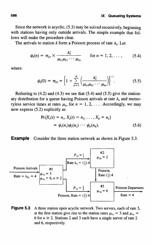
586 IX Queueing Systems
Since the network is acyclic, (5.3) may be solved recursively, beginningwith stations having only outside arrivals. The simple example that fol-lows will make the procedure clear.
The arrivals to station k form a Poisson process of rate Ak. Let
41k(n) = ITko XPkIPk2 ... Ak
where
(5.5)
Referring to (4.2) and (4.3) we see that (5.4) and (5.5) give the station-ary distribution for a queue having Poisson arrivals at rate Ak and memo-ryless service times at rates µk for n = 1, 2. .... Accordingly, we maynow express (5.2) explicitly as
Pr(X1(t) = n X2(t) = n2, . . . , XK = nk}
= 41,(n.)412(n2) ... 4K(nK) (5.6)
Example Consider the three station network as shown in Figure 5.3.
for n = 1, 2, ... , (5.4)
All
4'40) = ITko = {1 + 7, (,7=i \AAiAA-2 ... Ab,
Ak
P12-;
Poisson Arrivals
Rate = Xo, = 4
#1
µu=3µ,,,=6,n?2
JRateX2= (;) 4
Poisson, Rate = () 4
#2
µ2 = 2
IPoisson,Rate (;) 4
#3
µs = 6Poisson Departures
Rate = 4
Figure 5.3 A three station open acyclic network. Two servers, each of rate 3,at the first station give rise to the station rates µ = 3 and µ,, =6 for n ? 2. Stations 2 and 3 each have a single server of rate 2and 6, respectively.

5. Open Acyclic Queueing Networks 587
The first step in analyzing the example is to determine the arrival ratesat the various stations. In equilibrium, the arrival rate at a station mustequal its departure rate, as asserted in (d). Accordingly, departures fromstate 1 occur at rate A, = 4, and since these departures independently travelto stations 2 and 3 with respective probabilities P,, = and P13 = , we de-termine the arrival rate A2 = (104. At station 3 the arrivals include boththose from station 1 and those from station 2. Thus A3 = ()4 + (1)4 = 4.
Having determined the arrival rates at each station, we turn to deter-mining the equilibrium probabilities. Station I is an M/M/2 system withA = 4 and µ = 3. From (2.16), or (5.4) and (5.5), we obtain
llPr{X,(t)=0}=7ro={1+(31+2
2(1/3)
-i=0.2
and
(42)
(0 f = 1.
3/ or n ,
Pr{X1(t) = n} =(0.4)
2
( )"for n ? 2
3.
Station 2 is an M/M/1 system with A = and µ = 2. From (2.9) we obtain
Pr(X2(t) = n) = (--)(--) for n = 0, 1, ... .
Similarly station 3 is an M/M/1 system with A = 4 and µ = 6, so that (2.9)yields
Pr{X3(t)=n} =(3)(3) for n = 0,1.....
Finally, according to Property (a), the queue lengths X#), K,(t), andX3(t) are independent, so that
Pr{X1(t) = n,, X2(t) = n2, X3(t) = n3)
= Pr{X1(t) = n,} Pr(X2(t) = n,} Pr{X3(t) = n3}.

588 IX Queueing Systems
5.4. Appendix: Time Reversibility
Let {X(t), -oo < t < +co} be an arbitrary countable-state Markov chainhaving a stationary distribution Tr; = Pr{X(t) = j} for all states j and alltimes t. Note that the time index set is the whole real line. We view theprocess as having begun indefinitely far in the past, so that it now isevolving in a stationary manner. Let Y(t) = X(- t) be the same process, butwith time reversed. The stationary process {X(t)} is said to be time re-versible if { X(t) } and { Y(t) } have the same probability laws. Clearly,Pr { X(0) = j) = Pr { Y(O) = j) = ir;, and it is not difficult to show that bothprocesses are Markov. Hence, in order to show that they share the sameprobability laws it suffices to show that they have the same transitionprobabilities. Let
P;(t) = Pr{X(t) = jIX(0) = i},
Qi;(t)=Pr{Y(t)=jlY(0)=i).
The process {X(t)} is reversible if
/Pj (t) = Qij (t)
for all states i, j and all times t. We evaluate Qi;(t) as follows:
Qi; (t) = Pr{Y(t) = jI Y(0) = i }
= Pr{X(-t) = i1 X(0) = i }
= Pr{X(0) = jIX(t) = i} (by stationarity)
Pr{X(t) = i}
Pr{X(0) = j, X(t) = i}
IT; Pi(t)
IT,
.
(5.7)
In conjunction with (5.7) we see that the process {X(t)} is reversible if
F,(t) = Q11(t) = 'Pi(t)iTi
or
ii I;(t) = ;Pi(t), (5.8)
S. Open Acyclic oueueing Networks 589
for all states i, j and all times t.As a last step, we determine a criterion for reversibility in terms of the
infinitesimal parameters
a;; = lim1I Pr{X(t) = AX(o) = i }, i 0 j.
110 t
It is immediate that (5.8) holds when i = j. When i 0 j,
P;(t) = at + o(t),
which substituted into (5.8) gives
1rJa;;t + o(t)] = ir;[a;;t + o(t)],
(5.9)
and after dividing by t and letting t vanish, we obtain the criterion
'zr,a;j = ir1a;; for all i 0 j. (5.10)
When the transition probabilities are determined by the infinitesimal pa-rameters, we deduce that the process {X(t)} is time reversible whenever(5.10) holds.
All birth and death processes satisfying VI, (3.5) and having stationarydistributions are time reversible! Because birth and death processes have
a,.1+I = A.,
a;.;-1 = µr,
and
a;.l=0 ifli - jj> 1,
in verifying (5.10) it suffices to check that
or
But [see VI, (4.6) and (4.7)],
for i = 0, 1, .... (5.11)
Jy0A, A;-,1r;=aro fori=l,2,...,
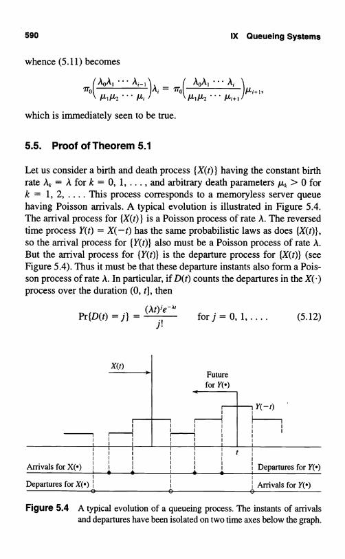
590 IX Queueing Systems
whence (5.11) becomes
1TO ( Alp-- , , * A)Ai = 'To
which is immediately seen to be true.
5.5. Proof of Theorem 5.1
AOA, ... A,1
Al P-2 N+ I
Let us consider a birth and death process {X(t)} having the constant birthrate Ak = A for k = 0, 1, ... , and arbitrary death parameters lµk > 0 fork = 1, 2, .... This process corresponds to a memoryless server queuehaving Poisson arrivals. A typical evolution is illustrated in Figure 5.4.The arrival process for {X(t) } is a Poisson process of rate A. The reversedtime process Y(t) = X(-t) has the same probabilistic laws as does {X(t)},so the arrival process for {Y(t)} also must be a Poisson process of rate A.But the arrival process for {Y(t)} is the departure process for {X(t)} (seeFigure 5.4). Thus it must be that these departure instants also form a Pois-son process of rate A. In particular, if D(t) counts the departures in theprocess over the duration (0, t], then
Pr{D(t) = j} =(At)'e-A,
for j = 0 .... (5.12)1, ,j!
X(t)
,
,
,
i
Futurefor
Arrivals fori + + +
t
Departures for
Departures for1 1
Arrivals fore
Figure 5.4 A typical evolution of a queueing process. The instants of arrivalsand departures have been isolated on two time axes below the graph.
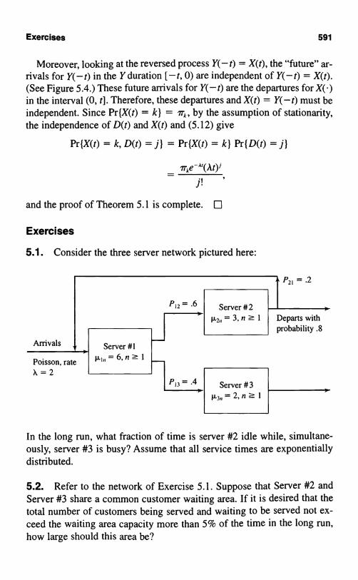
Exercises 591
Moreover, looking at the reversed process Y(- t) = X(t), the "future" ar-rivals for Y(-t) in the Yduration [-t, 0) are independent of Y(-t) = X(t).(See Figure 5.4.) These future arrivals for Y(-t) are the departures forin the interval (0, t}. Therefore, these departures and X(t) = Y(-t) must beindependent. Since Pr{X(t) = k} = lrk, by the assumption of stationarity,the independence of D(t) and X(t) and (5.12) give
Pr{X(t) = k, D(t) = j} = Pr (X(t) = k} Pr ( D(t) j)
1rke-`(At)!
and the proof of Theorem 5.1 is complete.
Exercises
5.1. Consider the three server network pictured here:
P21 = .2
P12 =
Arrivals
Poisson, rateX=2
Server #11
Server #2=3,n?1
Server # 31
Departs withprobability .8
ip.
In the long run, what fraction of time is server #2 idle while, simultane-ously, server #3 is busy? Assume that all service times are exponentiallydistributed.
5.2. Refer to the network of Exercise 5.1. Suppose that Server #2 andServer #3 share a common customer waiting area. If it is desired that thetotal number of customers being served and waiting to be served not ex-ceed the waiting area capacity more than 5% of the time in the long run,how large should this area be?

592 IX Gueueing Systems
Problems
5.1. Suppose three service stations are arranged in tandem so that thedepartures from one form the arrivals for the next. The arrivals to the firststation are a Poisson process of rate A = 10 per hour. Each station has asingle server, and the three service rates are µ, = 12 per hour, p, = 20 perhour, and p, = 15 per hour. In-process storage is being planned for sta-tion 3. What capacity C3 must be provided if in the long run, the proba-bility of exceeding C3 is to be less than or equal to 1 percent? That is, whatis the smallest number C3 = c for which lim,, Pr{X3(t) > c} : 0.01?
6. General Open Networks
The preceding section covered certain memoryless queueing networks inwhich a customer could visit any particular server at most once. With thisassumption, the departures from any service station formed a Poissonprocess that was independent of the number of customers at that station insteady state. As a consequence, the numbers X,(t), X2(t), ... , XK(t) of cus-tomers at the K stations were independent random variables, and the prod-uct form solution expressed in (5.2) prevailed.
The situation where a customer can visit a server more than once ismore subtle. On the one hand, many flows in the network are no longerPoisson. On the other hand, rather surprisingly, the product form solutionof (5.2) remains valid.
Example To begin our explanation, let us first reexamine the simplefeedback model of Section 4.3. The flow is depicted in Figure 6.1. The ar-rival process is Poisson, but the input to the server is not. (The distinctionbetween the arrival and input processes is made in Figures 1.2 and 4.1.)
FeedbackNot Poisson
Arrivals
Poisson X
Input
Not Poisson
Output
Feedback withprobability p
Depart with probability q
Poisson Departures
Rate = XNot Poisson
Figure 6.1 A single server with feedback.

6. General Open Networks 593
The output process, as shown in Figure 6.1, is not Poisson, nor is it inde-pendent of the number of customers in the system. Recall that each cus-tomer in the output is fed back with probability p and departs with prob-ability q = 1 - p. In view of this non-Poisson behavior, it is remarkablethat the distribution of the number of customers in the system is the sameas that in a Poisson M/M/1 system whose input rate is A/q and whose ser-vice rate is p,, as verified in (4.4).
Example Let us verify the product form solution in a slightly morecomplex two server network, depicted in Figure 6.2.
Server #2
P2
Arrivals
Poisson, rate X
Server #1
Wi
Feedback with
probability p
Depart withprobability q
Figure 6.2 A two server feedback system. For example, server #2 in this sys-tem might be an inspector returning a fraction p of the output forrework.
If we let X;(t) denote the number of customers at station i at time t, fori = 1, 2, then X(t) = [X,(t), X2(t)] is a Markov chain whose transition ratesare given in the following table:
FromState
ToState
TransitionRate Description
(m, n) (m + 1, n) A Arrival of new customer(m, n) (m + 1, n - 1) µ, Input of feedback customern?1(m, n) (m - 1, n) qµ, Departure of customerm?1(m, n) (m - 1, n + 1) pµ, Feedback to server #2m?1
594 IX Queueing Systems
Let ir,,,,, = lim,,,. Pr(X1(t) = m, X2(t) = n} be the stationary distribu-tion of the process. Reasoning analogous to that of (6.11) and (6.12) of VI(where the theory was developed for finite-state Markov chains) leads tothe following equations for the stationary distribution:
Air00 = g1.1ir1.0, (6.1)
(A + jx2)ir0.,, = PP'Iii.,,-1 + gp1iT1.,,, n ? 1, (6.2)
(A + Air,,,-1.0 + gj 1ir,,+1.0 + 1.1,
m ? 1, (6.3)
(A + A, + AlT,,-i.,, + p1x11;m+1.,,-1 + qp 1 irn,+;.,,
+ m, n ? 1. (6.4)
The mass balance interpretation as explained following (6.12) in VImay help motivate (6.1) through (6.4). For example, the left side in (6.1)measures the total rate of flow out of state (0, 0) and is jointly proportionalto ir0.0, the long run fraction of time the process is in state (0, 0), and A,the (conditional) transition rate out of (0, 0). Similarly, the right side of(6.1) measures the total rate of flow into state (0, 0).
Using the product form solution in the acyclic case, we will "guess" asolution and then verify that our guess indeed satisfies (6.1) through (6.4).First we need to determine the input rate, call it A1, to server #1. In equi-librium, the output rate must equal the input rate, and of this output, thefraction p is returned to join the new arrivals after visiting server #2. Wehave
Input Rate = New Arrivals + Feedback,
which translates into
A, = A + pA,
or
A AA,=1-pq (6.5)
The input rate to server #2 is

6. General Open Networks 595
AA2 = pA, = q (6.6)
The solution that we guess is to treat server #1 and server #2 as inde-pendent M/M/1 systems having intput rates A, and A2, respectively (eventhough we know from our earlier discussion that the input to server #2,while of rate A2, is not Poisson). That is, we attempt a solution of the form
A,
- ')(' "A I A P12 P12 )
- (1
In
It is immediate that
form,n? 1.
(6.7)
W W
77 1Tirr.n = 1,n=0n=0
provided that A, = (A/q) < µ, and A2 = pAlq < p.2.We turn to verifying (6.1) through (6.4). Let (Algµ,)m X
(pA1gµ2)". It suffices to verify that 0,,,,, satisfies (6.1) through (6.4), sinceand 6,,,,, differ only by the constant multiple iro,,, = 1 - A,/µ,) X
(1 - A2/µ2). Thus we proceed to substitute 9,,,,,, into (6.1) through (6.4) andverify that equality is obtained.
We verify (6.1):
A=q,.lqµ,
=A.
We verify (6.2):
(A+
+11 - qk
or after dividing by (pA/gµ2)" and simplifying,
A+µ2=\pq1\pAI+A=A+µ2.

596 IX Queueing Systems
We verify (6.3):
(A +µ)(qµ,
)_ AI + I,,,+i +
(P, qlu,)'(gp-z
1'
which, after dividing by (A/qµ,)"', becomes
(A+µ0_A(q +gA,( )gµj +µ\gJ11)(q )'
or
A+µ, =glxl +A+plL,, = A+ µ,.
The final verification, that 9satisfies (6.4), is left to the reader as Ex-ercise 6.1.
6.1. The General Open Network
Consider an open queueing network having K service stations, and letXk(t) denote the number of customers at station k at time t. We assume that
1. The arrivals from outside the network to distinct servers form inde-pendent Poisson processes, where the outside arrivals to station koccur at rate A.
2. The departures from distinct servers independently travel instantlyto other servers, or leave the system, with fixed probabilities, wherethe probability that a departure from station j travels to station k is
Pik3. The service times are memoryless, or Markov, in the sense that
Pr{Server #k completes a service in (t, t + ot]!Xk(t) = n)
= o(Ot) for n = 1, 2, ... , (6.8)
and does not otherwise depend on the past.4. The system is in statistical equilibrium (stationary).

6. General Open Networks 597
5. The system is completely open in that all customers in the systemeventually leave.
Let Ak be the rate of input at station k. The input at station k is composedof customers entering from outside the system, at rate Aok, plus customerstraveling from (possibly) other stations. The input to station k from stationj occurs at rate A;Pk, whence, as in (5.3),
xAk= AOk+ Z, A/P;k fork= 1,...,K. (6.9)
j=1
Condition 5 above, that all entering customers eventually leave, ensuresthat (6.9) has a unique solution.
With A...... A, given by (6.9), the main result is the product formsolution
Pr{X1(t) = n,, X2(t) = n,, . . . , Xk(t) = ng}
= i/i1(n1)Y'2(n2) ... Y'K(nK)+
where
(6.10)
t / i k ( n ) =T l k O A k for n = 1, 2, ... , (6.11)I
I /2'k2 * * * Pin
and
All
410) _ 1rkO = { 1+ k
t .
(6.12)n=I l-'i'k1P'k2 Alai
Example The example of Figure 6.1 (see also Section 4.3) correspondsto K = 1 (a single service station) for which P = p < 1. The external ar-rivals are at rate A,, = A, and (6.9) becomes
A, = Ao, + AP,,, or A, = A + A,p,
which gives A, = A/(1 - p) = A/q. Since the example concerns a singleserver, then = µ for all n, and (6.11) becomes
41(n) = ?l10(µ\n
=1110
`
)n'
qlA
598 IX Oueueing Systems
where
IT,o = I - -),9µ
in agreement with (4.4).
Example Consider next the two server example depicted in Figure 6.2.The data given there furnish the following information:
A01=A, A02=0,
P11 = 0, P12 = p,
P21 = 1, P22 = 0,
which substituted into (6.9) gives
A, = A + A2(1),
A2=0+A1(p),
which readily yields
A, _A
and AZ =PA
q q
in agreement with (6.5) and (6.6). It is readily seen that the product solu-tion of (6.10) through (6.12) is identical with (6.7), which was directlyverified as the solution in this example.
Exercises
6.1. In the case m ? 1, n ? 1, verify that 9as given following (6.7)satisfies the equation for the stationary distribution (6.4).
Problems
6.1. Consider the three server network pictured here:

Problems 599
P21 = .2
Arrivals j Server #1
µIn=6,n? 1
P12 = Server # 2
1L2n=3,n?1 Departs withprobability .8
Poisson, rate1=2
LPI Server #3
µ3n=2,n?1
1.
In the long run, what fraction of the time is server #2 idle while, simulta-neously, server #3 is busy? Assume that the system satisfies assumptions(1) through (5) of a general open network.


Further Reading
Elementary Textbooks
Breiman, L. Probability and Stochastic Processes with a View TowardApplications. Boston: Houghton Mifflin, 1969.
Cinlar, E. Introduction to Stochastic Processes. Englewood Cliffs, N.J.:Prentice-Hall, 1975.
Cox, D. R., and H. D. Miller. The Theory of Stochastic Processes. NewYork: John Wiley & Sons, 1965.
Hoel, R. G., S. C. Port, and C. J. Stone. Introduction to Stochastic Processes.Boston: Houghton Mifflin, 1972.
Kemeny, J. G., and J. L. Snell. Finite Markov Chains. New York: Van Nos-trand Reinhold, 1960.
Intermediate Textbooks
Bhat, U. N. Elements of Applied Stochastic Processes. New York: JohnWiley & Sons, 1972.
Breiman, L. Probability. Reading, Mass.: Addison-Wesley, 1968.Dynkin, E. B., and A. A. Yushkevich. Markov Processes: Theorems and
Problems. New York: Plenum, 1969.Feller, W. An Introduction to Probability Theory and Its Applications. 2 vols.
New York: John Wiley & Sons, 1966 (vol. 2), 1968 (vol. 1, 3rd ed.).Karlin, S., and H. M. Taylor. A First Course in Stochastic Processes. New
York: Academic Press, 1975.Karlin, S., and H. M. Taylor. A Second Course in Stochastic Processes. New
York: Academic Press, 1981.
602 Further Readings
Kemeny, J. G., J. L. Snell, and A. W. Knapp. Denumerable Markov Chains.New York: Van Nostrand Reinhold, 1966.
Ross, S. M. Stochastic Processes. New York: John Wiley & Sons, 1983.Ross, S. M. Introduction to Probability Models, 5/e New York: Academic
Press, 1993.
Renewal Theory
Kingman, J. F. C. Regenerative Phenomena. New York: John Wiley & Sons,1972.
Queueing Processes
Kleinrock, L. Queueing Systems. Vol. 1, Theory. Vol. 2, Computer Applica-tions. New York: John Wiley & Sons, Interscience, 1976.
Branching Processes
Athreya, K. B., and P. Ney. Branching Processes. New York: Springer-Verlag, 1970.
Harris, T. The Theory of Branching Processes. New York: Springer-Verlag,1963.
Stochastic Models
Bartholomew, D. J. Stochastic Models for Social Processes. New York: JohnWiley & Sons, 1967.
Bartlett, M. S. Stochastic Population Models in Ecology and Epidemiology.New York: John Wiley & Sons, 1960.
Goel, N. S., and N. Richter-Dyn. Stochastic Models in Biology. New York:Academic Press, 1974.
Point Processes
Lewis, P. A. Stochastic Point Processes: Statistical Analysis, Theory, andApplications. New York: John Wiley & Sons, Interscience, 1972.

Answers to Exercises
Chapter I
2.1. Because B and B` are disjoint events whose union is the whole sam-ple space, the law of total probability (Section 2.1) applies to give the de-sired formula.
2.3. (b)Ax) for x s 0;f(x) = 3x2 for 0 < x < 1;
0 for x > 1.
(c) E[X] - 1(d) Pr( X<_1}
2.4. (b) E[Z] _ $.(c) Var[Z] = 6;.
- 2664,
2.7. (a) 0 for x < 0;FX(x) = xR for O s x s l;
1 for 1 < x.
(b) E[X] = R/(1 + R).(c) Var[X] = R/[(R + 2)(R + 1)2].
2.8. f(v) = A(1 - v)A-' for O s v s 1;E[V]=1/(A+ 1);Var[V] = A/[(A + 2)(A + 1)2].

604 Answers to Exercises
2.9. 0 for x < 0;x2
FX(x)
for x
1; Var[X] = 16-
3.1. Pr{X = 3} = ;2.
3.2. Pr {0 defective) = 0.3151.Pr{0 or 1 defective) = 0.9139.
3.3. Pr{N = 10) = 0.0315.
3.4. Pr{X=2} =2e-2=0.2707.Pr(Xs 2) = 5e-22= 0.6767.
3.5. Pr{X ? 81 = 0.1334.
3.6. (a) Mean = n 2 1; Variance =
(b) m + 1I n-
Pr{Z=m}= 2n+1-mn2
(c) Pr{U = k} =1 +2(n-k)
(n + 1)2
4.1. Pr{X>1.5}=e3=0.0498.Pr{X = 1.5) = 0.
4.2. Median = log 2; Mean = .
n2 - 112
form=0,...,n;
for m = n + 1, ..., 2n.
for k=0,...,n.
4.3. Exponential distribution with parameter A/2.54.
4.4. Mean = 0; Variance = 1.

Answers to Exercises 605
4.5. a*Qy - PO'xQY
uX + 02 2po-xv,.for p ±1.
4.6. (a) f,.(y) = e-, for y,::> 0.
1 1c- iv
(b) f,,(w) =n
(w) for 0 < w < 1.
4.7. ^ as the gamma density fR(r) = A2re-Ar for r > 0.
5.1. Pr{X ? 1 } = 0.6835938Pr{X > 2) = 0.2617188Pr{X? 31 = 0.0507812Pr { X ? 4) = 0.0039062.
5.2. Mean = ;.
5.3. E[X] _ .
5.4. (a) E[X,,] = E[XB] = 3(b) E[min{XA, XB}] = s;(c) Pr{X,, < XB) = 5;(d) E[XB - XAjXA < XB] _ ;.
5.5. (a) Pr{Naomi is last) = ;;(b) Pr{Naomi is last) _ 2 = 0.1128;.,j'
(c) c = 2 + N/-3.
Chapter II
1.1. Pr{N=3,X=2} =,=6;Pr{X=5} =48;E[X] = '-.
1.2. Pr(2 nickel heads N = 4}
1.3. Pr{X > 1IX ? 1 } = 0.122184;Pr { X > 1 lAce of spades) = 0.433513.

606 Answers to Exercises
1.4. Pr{X = 21 = 0.2204.
1.5. E[XI X is odd] = A eAA CA
+ e-A)'
1.6. Pr{U=u,Zz}p2(1-p)z, O u:!:-: z;
Pr{U = uIZ = n}1
=n 1 1,
O: u :5 n.
2.1. Pr{Game ends in a 4} = o.
2.3. Pr(Win) = 0.468984.
3.1. k Pr{Z = k} E[Z] =;;
0 0.16406 Var[Z] = 1.604167.1 0.312502 0.257813 0.166674 0.075525 0.020836 0.00260
3.2. E[Z] = Var[Z] =8;
Pr{ Z = 2) = 0.29663.
3.3. E[Z] = A2; Var[Z] = µ(1 + µ)c72.
3.4. Pr{X = 2) = 0.2204;E[X] = 2.92024.
3.5. E[Z] = 6; Var[Z] = 26.
4.1. Pr{X= 2} _;.
4.2. Pr {System operates l = ;.
4.3. Pr{U > ;) = 1 - ;(1 + log 2) = 0.1534.
,(z) for 0 < z < oo.4.4.+
fz)2(1
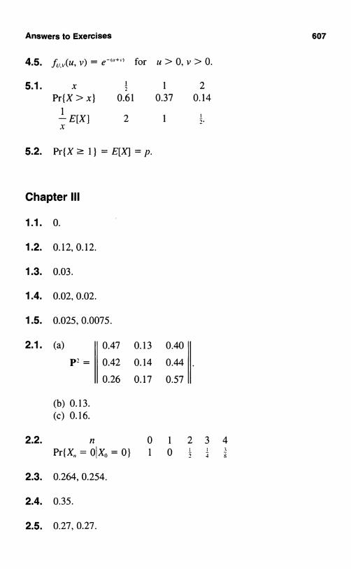
Answers to Exercises
4.5. f,.,,(u, v) = e-"""' for u > 0, v > 0.
5.1. X 1 2Pr{X > x} 0.61 0.37 0.14
1
- E[X] 2 1
x
5.2. Pr{X ? 1 } = E[X] = p.
Chapter III
1.1. 0.
1.2. 0.12, 0.12.
1.3. 0.03.
1.4. 0.02, 0.02.
1.5. 0.025, 0.0075.
2.1. (a) 0.47 0.13 0.40
P2 _ 0.42 0.14 0.44
0.26 0.17 0.57
(b) 0.13.(c) 0.16.
2.2. n 0 1 2 3 4Pr{X,, =OIX)=O} 1
0 ' '2 4
;s
2.3. 0.264, 0.254.
2.4. 0.35.
2.5. 0.27, 0.27.
607

608 Answers to Exercises
2.6. 0.42, 0.416.
3.1. -1 0 1 2 3
-1 0 0 0.3 0.3 0.4
0 0 0 0.3 0.3 0.4P=
1 0.3 0.3 0.4 0 0
2 0 0.3 0.3 0.4 0
3 0 0 0.3 0.3 0.4
23 (N l
..
P' NIP + N )q;
(N_ i)
P'', = (-)q.
3.3. -1 0 1 2 3
-1 0 0 0.1 0.4 0.5
0 0 0 0.1 0.4 0.5
P=1 0.1 0.4 0.5 0 0
2 0 0.1 0.4 0.5 0
3 0 0 0.1 0.4 0.5
3.4. -2 -1 0 1 2 3
2I-1 I 0 0 0.2
0 0 0.2
0.3
0.3
0.4 0.1
0.4 0.1
0 0 0 0.2 0.3 0.4 0.1
1 0.2 0.3 0.4 0.1 0 0
2 0 0.2 0.3 0.4 0.1 0
31 1 0 0 0.2 0.3 0.4 0.1

Answers to Exercises
3.5.0 1 2
I 1 0
' 0 '2 2
0 1 0
4.1. v03 = I*
4.2. (a) u,o=1;- s
.4.3. (a) u,o- = o105- ,o
(b) v, -T-
4.4. v0 = 6.
4.5. u = 'H,TT 3
(a)6.4.6. uI0 = 23
(b)- 'vl = 23
4.7. W- zo.
W. 2= 2s
-V,
as- ,,.
4.8. w = 1.290;w12=0.323v,=1.613.
4.9. u10 = zz = 0.40909Y,o = 0.17;P;o = 0.2658;P;o = 0.35762 . . .;P;0 = 0.40245 .
5.1. 0.71273.
609
5.2. (a) 0.8044; 0.99999928(b) 0.3578; 0.00288 .

610
5.3. p, =
P3 =
0.58 0.420.49 0.51
0.526 0.4740.553 0.447
P4_
P5 =
0.5422 0.45780.5341 0.4659
0.53734 0.462660.53977 0.46023
5.4. 0 1 2 3
0 0 0 1
5.5. PcO = 0.820022583.
5.6. 2.73.
5.7. u,o = 0.3797468.
5.8. po = a, ro = 1 - a;pi = a(l - /3), q, = /3(1 - a),r;=a(3+(1 -a)(1 -(3), for i? 1.
5.9. Po= 1,qo=0,p;=p,q;=q,r;=0 for i?1.
6.1. (a) u3s = ;
(b) uss = I 1 -(p)2J/L1
- I p ].
Answers to Exercises

Answers to Exercises
6.2. u,o=0.65.
6.3. v = 2152.777
6.4. v, = 2.1518987.
7.1.w
20 257t tJ
1o 40
I1 11
- .(a) u10
9-22;
(/b1 20. - 25\u) WII 11; W12 71
7.2.
w=100 70
79 79
30 100
79 79
30(.a) ulo 79;
(b) - 100. _ 70w - 79; W12 - 79
8.1. M(n) = 1, V(n) = n.
8.2. p.=b+2c;a2=b+4c-(b+2c)2.
8.3. n 1 2 3 4 5
UPI 0.5 0.625 0.695 0.742 0.775
8.4. M(n)=A",V(n)=A"(1-' ,JIB 1.
9.1. n 1 2 3 4 5
UPI 0.333 0.480 0.564 0.619 0.658ux = 0.82387.
9.2. cp(s) = Po + P2S2
9.3. cp(s)=p+qs".
9.4.(P(S) - (P(0)
1 - c4(0)
611

612
Chapter IV
610,7T 1 =
5, 1T,IT01.1 . - ? , 21
31 16 _ 1966 66 - 66,
1.3.1T I1 1'3
1.4. 2.94697.
1G 10 5 _ 9.5. 790 - 2 9 , 7r1 - 2 9 7 T 2 = 29, 1T 3 - 29
1.6. 1TOS
14,1f1A,
2
= 3- 14-
L40 - 40 - 135 1261.7. 7r0-441,1 441,192-441,193--
441
1.8. 7r = 177.
2 31.9. 1r0_
, I 71 72 7
171.10. irlatc 40
2.1. 1T,. = 9.
q2
2.2. One facility: Pr (Idle) =1 + p2'
Two facilities: Pr(Idle) =1
Answers to Exercises
l+p+p2'2.3. (a) p 0 0.02 0.04 0.06 0.08 0.10
AFI 0.10 0.11 0.12 0.13 0.14 0.16AOQ 0 0.018 0.036 0.054 0.072 0.090
(b) p 0 0.02 0.04 0.06 0.08 0.10AFI 0.20 0.23 0.27 0.32 0.37 0.42AOQ 0 0.016 0.032 0.048 0.064 0.080
2.4. p 0.05 0.10 0.15 0.20 0.25R, 0.998 0.990 0.978 0.962 0.941R, 0.998 0.991 0.981 0.968 0.952

Answers to Exercises
2.5. ITA=5.
2.6. ao = .
2.7. (a) 0.6831;(b) ir,=ar,=-0°,ir,=,',;(c) ?r3 = ,!,.
2.8. ?r 3 = 8SI
613
3.1. {n ? 1; P`"" > 01 = 15, 8, 10, 13, 15, 16, 18, 20, 21, 23, 24, 25, 26,28, ...)d(0) = 1, P`57' = 0, P;38' > 0 for all i, j.
3.2. Transient states: (0, 1, 31.Recurrent states: (2, 4, 5).
3.3. (a) (0, 2), { 1, 3), 14, 5);(b) (0), (5 ), ( 1, 2), (3, 4).
3.4. {0), d = 1;{1},d=0;{2,3,4,5},d= 1.
4.1. lr,=pkl(1 +p+p-+p;+p4) for k=0,...,4.
4.2. (a) ?r0 - -,4i99999
(b) m ,o 855010 - 1449
4.3. Iro=Ir,=0.2,7,=7r,=0.3.
5.1. lim P`"" = lim P`,"o' = 0.4;limP;o'= limPo'= 0;lim Pa'o = 0.4.
5.2. (a) (e) 3,(b) 0, (f) X,(c) 3I, (g) 5,(d) 9, (h) 27,

614 Answers to Exercises
Chapter V
1.1. (a) a-22;
(b) e2.
1.2. (pklpk-1) = A/k, k =0, 1, ... .
1.3. Pr{X = kI N = n} _ ()p*(1- p)"kAt
"e a1.4.
(a) ( ) k 0,1,...;k!
p=a
a+/3
(b) Pr{X(t) = n + kIX(s) = n) =Wt - s)]
E[X(t)X(s)] = Alts + As. k!
1.5. Pr{X = k} = (1 - p)pk for k = 0, 1, ... where p = 1/(1 + 0).
1.6. (a) a-12;(b) Exponential, parameter A = 3.
1.7. (a) 2e-2;64 -6.(b) e ,
(c) (6,)(1)2(2)4;3 3
(d) 32e-4
1.8. (a) 5e-22;
(b) 4e-4;1 - 3e-2
(c) 1 - e-2
1.9. (a) 4;(b) 6;(c) 10.
2.1. k 0 1 2(a) 0.290 0.370 0.225(b) 0.296 0.366 0.221
(c) 0.301 0.361 0.217

Answers to Exercises 615
2.2. Law of rare events, e.g. (a) Many potential customers who couldenter store, small probability for each to actually enter.
2.3. The number of distinct pairs is large; the probability of any partic-ular pair being in sample is small.
2.4. Pr{Three pa9f s error free) - e-''-.
3.1. a-6.
3.2. (a) e-' - e-";(b) 4e-'.
3.3. ;.
3.4.
3.5.
()()'(3)' = xsTI
3.6. F(t) = (1
3.7. t + 2 .
A
3.8. (i5)(2)S( )'.
3.9. Pr{W,.<_t}=1-
4.1.
4.2.
n+l4.
m=0,1, ,n.
I (At)Ae-Ar
7, k!
4.3. .
4.4. See equation (4.7).
4.5. [1-enl5
aJI

616
5.1. 0.9380.
5.2. 0.05216.
5.3. 0.1548.
6.1. 0.0205.
6.2. Mean= t, Variance =
6.3.
e-AC(z)t - e- At
1 - e-At
6.4. (a) 1;
(b) I-IIzr
2At
02
Answers to Exercises
A(t)ke-ACn
6.5. Pr{M(t) = k} =k!
where A(t) =AJ
[1 - G(u)] du.0
Chapter VI
Po(t) = e-';P1e-' - I -3t.
I(t) = z ze ,
P2(t) = 3[1e-' + Ze-3r - 1e-2t]
P3(t) = 6[8e-t + ;e-3t - 3e-zr - z4e-St].
1.2. (a) 6i(b) 2s.
6+36
C 36-
1.3. X(t) is a Markov process (memoryless property of exponential dis-tribution) for which the sojourn time in state k is exponentiallydistributed with parameter Ak.
1.4. (a) Pr {X = 01 = (1 - ah)" = 1 -nah + o(h);(b) Pr{X = 1) = nah(1 - ah)" = nah + o(h);(c) Pr{X ? 2) = 1 - Pr{X = 0) - Pr(X - 11 = o(h).

Answers to Exercises 617
1.5. E[X(t)] _ -, Var[X(t)] = 1 2P where P = e
P
1.6. (a) P,(t) = e-S;(b) P2(t) = 5[Ze-3r - lie-5']
(c) P3(t) = 15[zoe-3r - i6e-5' + -Le-13r].80
2.1. P3(t) = e-Sr;P2(t) = [3e-2r - 3e-S7;
PI(t) = 10[be-5r + ;e-2r - Ze-3r]
Pa(t) = 1 - P,(t) - NO - NO-
2.2. (a) io;(b) 29'15+
(c) 361
900
2.3. P3(t)=e ;P2(t) = [e_, - e-2,];
pi(t) = 2[i e_' - e-2r + 1e-31];
Po(t) = 1 - PI(t) - NO - P3(t).
2.4. P2(t) = 10e-41(l - e-2')3
3.1. for n=0,1,....
3.2. Assume that Pr{ Particular patient exits in [t, t + h)lk patients }
1h + o(h).Mk
4.2. ar. =a
k -Ik
(Npk(l - P)"-k where p =a +
4.3. 1k
a= where A -
4 .4 . (a) aro=1/(1+µ+2(µ)I;
(b) am = 1/(1 + +(-)2).
4.5. ark = (k + 1)(1 - 0)29'`
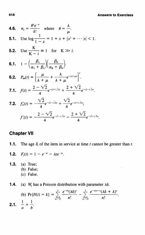
618
x
4.6. 7r, =k!
where 0 = -.µ
5.1. Use log 1 = 1 + x + x2 +1x5.2. Use
K= 1 for K >> i.
K - i
6.1. 1
e-(A+µ)r16.2. P,(t) = A + µ + A + µ J
7.1.
7.2.
< 1.
f(t) =2 - e a+\2u + 2 +
e-(2-'2),
4
--e -(2-\ 2)1 +° 4
A
4
4
Answers to Exercises
- _ -e-c-\2)t - 2 +
e-(,+v2,r2
4 4
Chapter VII
1.1. The age S, of the item in service at time t cannot be greater than t.
1.2. F,(t) = 1 - e-A, - Ate-A,
1.3. (a) True;(b) False;(c) False.
1.4. (a) W has a Poisson distribution with parameter Ak.
(b) Pr(N(t) = k} _
2.1. a + b.
9Ae-o
I
n=0
e-"A(Ak)" e-A(A+I)(Ak + A)
n! , n!
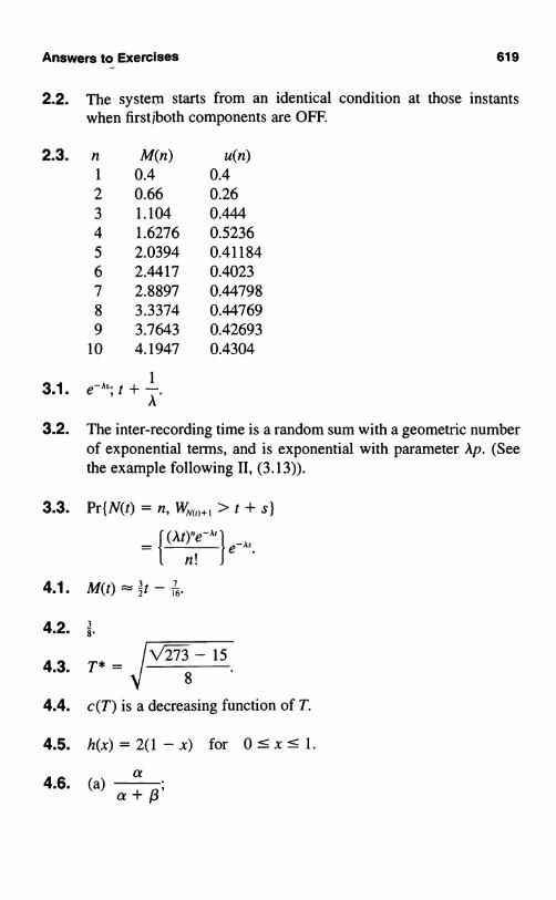
Answers to Exercises 619
2.2. The system starts from an identical condition at those instantswhen first ;both components are OFF.
2.3. n M(n) u(n)
1 0.4 0.4
2 0.66 0.263 1.104 0.4444 1.6276 0.52365 2.0394 0.411846 2.4417 0.40237 2.8897 0.447988 3.3374 0.447699 3.7643 0.42693
10 4.1947 0.4304
3.1. a-";t +1
A
3.2. The inter-recording time is a random sum with a geometric numberof exponential terms, and is exponential with parameter Ap. (Seethe example following II, (3.13)).
3.3. Pr f N(t) = , WN(,) , > t + S)
= {_(At)"e'le-As.
n!
4.1. M(t) = Zt - 6.
4.2. 8.
- 154.3. T* = 8
4.4. c(T) is a decreasing function of T.
4.5. h(x) = 2(1 - x) for 0 : x < 1.
4.6. (a)a
;a+p

620 Answers to Exercises
/LA15 ..
1
5.2. 9
5.3. T* = cc.
6.1.-6.2. n0 0.6667 1.33333
1 1.1111 0.888882 0.96296 1.03704
3 1.01235 0.987654 0.99588 1.00412
5 1.00137 0.998636 0.99954 1.000467 1.00015 0.999858 0.99995 1.00005
9 1.00002 0.9999810 0.99999 1.00001
6.3. E[X] = 1; 1 bk = 1.
Chapter VIII
1.1. (a) 0.8413.(b) 4.846.
1.2. Cov[W(s), W(t)] = min{s, t}.
1.3. ap = ',_cp(z)t-'[z2 - 1];
ax= r zcp(z).

Answers to Exercises 621
1.4. (a) 0.(b) 3u2 + 3iuv + uw.
1.5. (a) a-'-`;(b) t(1 -s) for 0 < t < s < 1;(c) min{s, t}.
1.6. (a) Normal, .t = 0, U-z = 4u + v;(b) Normal, A=0,o-'-=9u+4v+w.S
1.7.S
2.1. (a) 0.6826.(b) 4.935.
2.2. If tan 0 = V, then cos 0 = t/(.
2.3. 0.90.
2.4. Reflection principle: Pr(M,, ? a, S,, < a) _Pr{M ? a, S,, > a}(= Pr(S,, > a)).Also, Pr{M ? a, S = a) = Pr(S = a).
2.5. Pr(,r0<t) =Pr{B(u) 00 forallt<-u<a} = 1 - t9(t,a).
2.6. Pr{z, <t} = Pr(B(u) = 0 for some u, b < u < t).
3.1. Pr(R(t) < yIR(0) = x)= Pr(-y < B(t) < yIB(0) = x}= Pr{B(t) < yIB(0) = x} - Pr{B(t) < -yIB(0) = x).
3.2. 0.3174, 0.15735.
3.3. 0.83995.
3.4. 0.13534.
3.5. No, No.

622
4.1. 0.05.
4.2. 0.5125, 0.6225, 0.9933.
4.3. 0.25, 24.5, 986.6.
4.4. r = 43.3 versus E[T] = 21.2
4.5. 0.3325.x
Answers to Exercises
4.6. (a) E[( - a)+] = J xcp(x) dx - a f cp(x) dxa a
= cp(a) - a[ I - c1(a)]
(b) (X - b)+ = v( - b µ)+.Q
5.1. 0.8643, 0.7389, 0.7357.
5.2. 0.03144, 0.4602, 0.4920.
5.3. (a) (,1 - S)"vCoV[Vro i+k] _ (1 - 6)k.
(b) E[# V,, = v] _ -(3vVar[OVIV = v] = 1.
Chapter IX
1.1. (a) Probability waiting planes exceed available air space.(b) Mean number of cars in lot.
1.2. The standard deviation of the exponential distribution equals themean.
1.3. 11 days.
2.1. 2536

Answers to Exercises
2.3. L = 1 versus L = 5.
1 , 1 p3.1. v=-,z-=-, L
_ 1 - p
3.2. L= p+ p 2(1 + a)
2a(1 - p)
3.3. 3.
3.4. ;-' versus 3.
3.5. M(t) = AJ
[1 - G(y)] dy - Av.0
4.1. 8 per hour.
4.2. 16
4.3. 8.55.
4.4. 0.0647.
5.1. 15(4) 5
623
5.2. Pr{Z :5 201 = 0.9520


Index
Absorbed Brownian motion 499-502, 507Absorbing Markov chain 123-125Absorbing state 105, 120, 170
in birth and death process 379-384Absorption probability 165Absorption time 173
in birth and death process 382-384Accounts receivable model 167, 230Addition law 6Age 45, 422, 424, 425, 426
in a Poisson process 434in a renewal process 146limiting distribution of 443
Age replacement 45, 221-223, 438, 446Airline reservation model 234Aperiodic 239, 246Arrival process 590Astronomy application 314Availability 217, 228, 234, 403Average fraction inspected 220, 228Average outgoing quality 220, 228
Backward equations 359Bacteria 30, 289, 315Balking 567, 581Basic limit theorem of Markov chain 246Batch processing 150-151, 296Bernoulli distribution 24Bernoulli random variables sum of 280, 289Beta distribution 38, 83Beta function 55Bid model 69, 86, 149, 331Binary message 100, 104
Binomial distribution 25, 293convolution of 32
Binomial expansion 341Binomial theorem 55Bird problem 437Birth and death process 547
limiting distribution of 366-368postulates for 355-356with absorbing states 379-384
Birth process 333-339linear 346
Black-Scholes 516-521Block replacement 428-430, 432, 456Borel set 19Branching process 91, 177-195
multiple 192-195Brand switching model 229Breakdown rule 350, 354Brownian bridge 502, 522Brownian meander 504Brownian measure 534Brownian motion 474-479
absorbed 499-502geometric 514-516integrated 535maximum of 491-493, 513of pollen grain 473, 526reflected 498-499standard 478two dimensional 506with drift 508-511
Bum-in 403-405Busy period 551

626
Cable fatigue model 349-353, 354Cable strength model 483Call option 516, 523, 531Car problem 258Carrying capacity 386, 390Cash management 162-164, 488Central limit principle 483, 508, 533Central limit theorem 34, 75, 479Certain event 6Chapman-Kolmogorov equation 356, 394Chebyshev inequality 93Chemical reaction 354, 378Cigar problem 134-135Collards 365Communicate 235, 258Compound Poisson process 318-320Compression testing model 490Computer challenge 135, 168-169, 176,
290, 311, 490Computer coding 288Conditional
density function 71, 79dependence 85distribution function 71expectation 81expected value 60independence 85mass function 57probability 14
Continuous random variable 8Continuous sampling 218-221Control limit rule 225Convolution 12
of binomial distribution 32of geometric distribution 32of Poisson 268
Correlation coefficient 12, 22, 39, 85Counter model 427, 436Covariance 11, 86
matrix 481Covariance function 482
for Brownian bridge 507for Brownian motion 479of Ornstein-Uhlenbeck process 525
Index
Cox process 273-274, 408-411Crack failure model 64-68, 324, 343Craps 148Cumulative process 449, 451Current life, See ageCustomer waiting time 542
Damage 134Death process 345-349
linear 346-349Defects 274, 316Delayed renewal process 447Departure process 582, 590Detector model 310Dice
five before seven 134four before seven 65, 68shaved 66-68weighted 69-70
Differential equations 335, 337, 344, 415,523, 557
and limiting distribution 367backward 359for Cox process 409-410for M(t) 361for two state Markov chain 363forward 361, 367Kolmogorov 359, 361
Diffusion equation 475Discount factor 132, 300Discrete random variable 8Disease spread 99, 342Disjoint 6Dispatch model 278Dispersal of offspring 183Distribution function 7Do men have more sisters 64Doubly stochastic 206, 260
Poisson process 273
Ehrenfest urn model 108, 532-533, 539Electron multiplier model 78, 178Elementary renewal theorem 437Embedded Markov chain 396, 560, 563

Index
Embedded random walk 380Empirical distribution function 503Equal load sharing 351, 483Equally likely outcomes 3Excess life 115, 414, 422, 424, 425, 426,
462for Poisson process 433limiting distribution of 443
Expected value 9of sum 12
Exponential distribution 35-37, 46-50Extinction 345, 347, 355, 388-392
mean time to 385, 390-393Extinction probability 181-183, 384, 393
and generating function 187-190
Failure 446crack model for 324
Failure model 115Failure rate 36, 41, 350Fair game 88, 143Family name survival 179Family size 184, 195, 197Fatigue 324, 343, 349-353Fecundity model 125-127Feedback 569, 592Fiber, See filamentFibrous composite 316Filament, strength of 326-328, 411-413First come-first served 542, 239First return 240, 245First return
mean 255, 257First step analysis 101, 116-125, 169-174,
255,261-262,360,380infinitesimal 508, 509, 510
Five before seven 134Flashlight problem 52-53Flea beetle model 365, 557Forward equations 361, 367, 376, 409Four before seven 65, 68Fundamental matrix 172, 175
Gauge length 326
627
Gambler 90-91Gambler's ruin 94, 142, 144, 148, 152,
156, 509mean duration of 167
Gambling 22, 88, 94Game show 150Gamma distribution 38, 276, 291Gamma function 53Gaussian process 481, 506Gene frequency model 108-111, 179,
372-376,528-529Generating function 185, 276
and extinction probability 187-190and sums of rv's. 185, 190-192
Geometric Brownian motion 514-516Geometric distribution 25-26, 33, 339
convolution of 32generalized 33
Geometric series 56
Hazard rate 36, 350History 215-216Hitting probability 173Hitting time 152, 493, 509
mean of 165Home helicopter 342
Idle period 551Immigration 342, 361, 368Impossible event 6Impulse response function 304Imputed volatility 520Independent events 7Independent increments 270, 477Independent Poisson processes 321Independent random variables 11
defining a Markov chain 138-141Indicator
function 45of event 24random variable 21
Industrial mobility 398-402Infinitesimal first step analysis 508, 509,
510
628
Infinitesimal generator 356, 396Infinitesimal matrix 359Infinitesimal parameter 339Infinitesimal probability 333, 334, 395Input process 541Input rate 570Integral equation 338Integrated Brownian motion 535Intersection 6Invariance principle 480, 482, 488Inventory model 106-108, 112-113, 114,
115, 230Irreducible 246, 258Irreducible Markov chain 236Joint distribution I IL = A W 542-544Laplace transform 311, 414Last step analysis 360, 409Law of large numbers 4Law of rare events 27, 28, 279-286, 288Law of total probability 6-7, 14, 49, 58,
60, 65, 71, 72, 82, 87, 94, 101, 119,120, 121, 268, 335, 409, 458, 461,559
Lazy professor 457Learning model 297, 434Length biased sampling 436Limiting distribution 199, 254, 257, 377
and differential equations 367for birth and death process 466-468interpretation of 207of age and excess life 443-445
Limiting transition probability 212, 232Linear birth process, See Yule processLinear death process 346-349, 353, 355Linear growth 346
with immigration 361, 368Loaded dice 69-70Logistic process 371-372Lognormal distribution 35Long run relative frequency 4
M/G/l queue 545, 558-563M/G/c queue 564-565M/M/l queue 544, 548-552
Index
M/M/S queue 553-555, 556M/M/e queue 544,552-553,557Marginal distribution 1 IMarked Poisson process 321-324, 564Markov chain 95
embedded 396in continuous time 394-396two state 136-138, 200, 362-364,
396-398,407,431Markov inequality 88-89, 93Markov process 95Marlene, see also Martha 470Martha, see also Marlene 151Martingale 87-94, 151, 184, 297, 490,
507, 524systems theorems 88
Match 21Maximal inequality 89-90Maximum of Brownian motion 491-493,
513Maze 122-123, 131, 166Mean 9Measurable 17Median 9, 40Memoryless property 35, 48, 348, 585,
596Mode 31Moment 9Multinomial distribution 29-30
Naomi 51Negative binomial distribution 25-26, 59,
84Neutron chain reaction 178Normal distribution 34
bivariate 39conditional 86multivariate 40, 481notation for 475table of 486
Null recurrent 246
o(.) notation 9, 271-272, 276-277, 334,344
Offspring 73

Index
Optimal replacement model 224-228Option pricing 516-521Ornstein-Uhlenbeck process 524-538
and Brownian motion 525, 537stationary 532
Overflow 545, 570, 580
Partial sums 140-141, 176, 480Pattern search 114, 130Period of state 237Periodic 235, 254Peter principle 398-402, 450Planned replacement, See Age replace-
mentPoisson
decomposition 268-269sum of 268
Poisson counting process 290Poisson distribution 26-29, 196, 258,
267-268and uniform distribution 63convolution of 31
Poisson point process 290definition 284nonhomogeneous 323postulates for 282
Poisson process 270-273as a renewal process 427, 432-435compound 318-320doubly stochastic 273marked 321-324, 564mixed 273, 278nonhomogeneous 271-273postulates for 334, 344repositioning of 329spatial 311-314with Markov intensity 408-411
Population size model 70, 335, 339-341,341,346-349,371-372,384
with age structure 463-469Population stability 193Position process 530, 536Positive recurrent 246Preemptive priority 572-579, 580Premium 517
629
Priority, preemptive 572-579, 580Priority queue 545Probability density function 8Probability mass function 8Probability measure 15Probability of absorption 165Probability of extinction 181-183Probability space 16Process control 453Product form 592Production process 30, 100, 104, 148, 213,
218-221, 231Pure birth process, See birth processPure death process, See death process
Queue discipline 531Queueing model 70, 114, 450
discrete 111-112, 149Queueing network 545
general open 592-598open acyclic 581-591
Quiz show 84
Radioactive decay 294, 301, 364alpha particles 329
Random environment 84, 70-77Random sum 180
distribution of 74-75moments of 72
Random variable 7continuous 8discrete 8
Random walk 141-145, 151, 156-161,162, 480, 488, 489, 496
simple 145, 177Random walk hypothesis 318Recurrent 246Recurrent state 240, 241Reducible Markov chain 258-264Redundancy 216-218, 403-405Reflected Brownian motion 498-499Reflection principle 491-493, 497Regular Markov chain 199Regular transition matrix 199-205, 257Reliability model 216-218, 228, 234

630
Reneging 581Renewal argument 458Renewal equation 458Renewal function 421
for Poisson process 433Renewal process 146
definition 419delayed 447-448in Markov chain 428in queues 427stationary 448
Renewal theorem 441, 462, 551, 558elementary 439
Repair model 407Repairman model 369-371, 376, 377, 545,
546Replacement model 150, 221-228, 438,
450, 452optimal 224-228
Reservoir model 496, 506Risk theory 70, 318, 452-453Rumor spread 134
or-algebra 16Sample space 15Sampling
continuous 218-221length biased 434, 436sum quota 305-308, 435wildlife 71
Sequential decisions 511-513, 521, 522Sequential hypothesis test 513Server utilization 542Service distribution 531Shaved dice 66-68Shewart control chart 453Shock model 277, 278, 319, 328, 329Shot noise 304-305, 310, 311Sigma-algebra 16Size effect 325Social mobility 200, 210Sojourn 336, 357-359, 395, 447
in Poisson process 290, 292Spatial point process 311-314
Index
Spreadof disease 99, 342of rumor 134
Stable age distribution 469State space 5Stationary
Cox process 414distribution 247, 252, 256, 258, 366,
376-378intensity 409Ornstein-Uhlenbeck process 532renewal process 448-449transition probability 96
Sterile male insect control 388-392Stirling's formula 54Stochastic 2Stochastic process 5Stock prices 75-77, 88, 318, 474, 489,
506, 510, 514, 522, 531Stop and go traveler 366, 416-417Strength
compression 490of cable 483of filaments 326-328
Striking price 517Subjective probability 5Success runs 145-147, 165-166Successive maxima 138-140Sum quota sampling 305-308, 435Sums of numbers 56System 50-51, 231, 378, 379, 406, 407,
431,446, 456System throughput 542
Tail probability 43-46, 52, 422Tandem queues 583Tensile strength 411-413Time reversal 588-591Total life 422, 457
for Poisson process 434Tracking error 527Traffic flow 427Traffic intensity 549, 563, 573Transient state 120, 170, 235, 240, 241

Index
Transition probability 95for two state Markov 363-364limit of 212, 232matrix 96n-step 101regular 199-205stationary 96
Uncorrelated IIUniform distribution 37, 93, 290, 311
and 1 sisson process 297-299discrete 30
Union 6Urn 63, 91-93, 108, 113, 115, 132, 134,
168-169, 211
Variable service rates 569Variance 9Velocity 538Volatility 520
Waiting timein Poisson process 290, 296, 309in renewal process 420
Wald's approximation 513Warrant 516Wear 134Weather model 215-216, 232, 238,
455
Weibull distribution 486Weighted dice 69-70Weiner process 474Wildlife sampling 71
You Be the Judge 28-29Yule process 339-341, 342, 346
with immigration 342
Zero-seeking device 130, 175Zeros of Brownian motion 494-496,
497
631