an introduction to the benefits of optimization models for · an introduction to the benefits of...

May 15, 2006 1

An Introduction to the Benefits of Optimization Models for

Underwriting Portfolio Selection1

Jerome Kreuser2

Morton Lane3

Abstract

The use of optimizing models for portfolio selection and construction in the context of

insurance is relatively new. Investment portfolio managers regularly rely on optimization,

but underwriters are much more likely to use good old fashion trial and error, with some

admittedly quite sophisticated, simulation techniques to developing underwriting

portfolio strategies. The unique characteristics of insurance risk, e.g. long tails, one sided

correlations etc, did not lend themselves to early optimization models but, certain

technical breakthroughs have advanced optimization modeling and insurance risk is now

a potentially important application. Moreover, once adopted, optimization techniques

have considerable informational benefits over simulation.

The purpose of this paper is to illustrate these benefits. We do this in two ways.

First by tracing out the numerical implications with a simple practical application; second,

by introducing some of the algebra4 necessary to extract the benefits in more general and

complicated cases. The techniques have been successfully applied in several large scale

real situations and further technical details will be forthcoming in subsequent papers5.

1 We are grateful for the support of Renaissance Re and AIR Worldwide in the furtherance of this effort. 2 Executive Director of The RisKontrol Group, Bern, Switzerland. [email protected]. 3 President of Lane Financial LLC, Chicago, Illinois, USA: [email protected] 4 Non technical readers may wish to skip boxed sections containing mostly algebra. 5 Working titles “Capital allocation and risk in reinsurance”, and “Implied prices in reinsurance”.

May 15, 2006 2

Introduction

Maximizing expected returns among a set of alternatives is not difficult when

there is a limited amount of each deal available, even with limited capital; simply successively pick the one with the highest expected return and commit as much as possible until capital is exhausted. However, that stand-alone process can result in more risk than is acceptable. The portfolio may contain too great a chance of having a bad outcome and of losing lots of capital.

The stand-alone procedure may also fail to take advantage of any diversification and dependency possibilities that might reduce the chances of loss.

In short, portfolio selection in a risky environment requires not only a definition of objectives (for example, maximizing expected return) but also a definition of what potential losses are acceptable and with what frequency. Risk preferences must be specified. Risk preferences are generally expressed for the portfolio as a whole, not the individual deals. It, therefore, behooves managers to make selections in a portfolio context not just on a stand-alone basis. Portfolio optimization6 requires joint deal evaluation.

In this paper we will restrict ourselves to the insurance sector and selecting an optimal set of underwriting opportunities. Typically this selection is done so as to maximize expected returns on capital over a horizon of one year. We also focus on CVaR as our risk preference function, albeit at multiple levels. In order to illustrate the basics we will look at a portfolio underwriting selection problem in a relatively simple environment. The selection is among a dozen or so underwriting opportunities (deals) which are all exposed to Florida wind. Since the deals are all exposed to the same wind risk, the illustration will not address the benefits of horizontal diversification. (Comments on the diversification benefits are deferred to a latter section and a multi-zone risk environment.) Selection, nevertheless, is still a non-trivial problem. The deals must be chosen to satisfy risk preference constraints and the example will illustrate how these are handled. The internal workings and rationales implicit in the model will be teased out of the solution details.

We conclude by illustrating the powerful concept of “Implied Probabilities”, a.k.a. risk neutral probabilities or risk adjusted probabilities. It is arguable that this implied distribution is at least as valuable as the optimal solution itself. Commercial optimization models do not provide this information nor is it a feature that is directly obtainable from Dynamic Financial Analysis (DFA) nor simple Monte Carlo simulation. Jarrow (2005) gives a method for computing the implied probabilities. Our method is different and derives from the optimal solutions from the problem we describe in the next section.

6 The optimization model utilized herein is a proprietary model system – RisKontroller ReALTM

(RisKontroller Reinsurance Asset Liability Optimizer). The approach embedded in RisKontroller ReAL, is

Dynamic Stochastic Programming (DSP), which can be used in a variety of applications. Other examples

of Dynamic Stochastic Programming applications can be found in Ziemba and Mulvey (1998).

May 15, 2006 3

1. The Problem

The basic problem is to maximize expected returns among specified deals, subject to risk preference constraints, practical deal size constraints, special constraints on retrocessions, and a capital limit. In our example here we will use a capital limit of $100 million. In general we separate deal variables and ceded variables because they may have different kinds of constraints on each one rather than treating them as “shorted” variables. The list of model variables and inputs is given in the following tables:

Model Inputs

Name Identification

bda Bid/ask spread.

kc Confidence level expressed as a decimal for risk level k

capital Starting capital

kcvar Percent limit on loss of capital for risk level k

,i jloss Unit loss of deal j in scenario i

jprice Price of deal j as a percent

i! Probability of scenario i

rate Rate of return on investments

tm Percentage of capital as limit on total ceded premiums

trs Transaction costs as a percent

Decision Variables Determined by Model

Name Identification

k! Alpha value for risk k, which turns out to be VaR for active

constraints

jdeal Amount of premium of deal j written

0funds Beginning period funds net of capital

1ifunds End-of-period funds net of capital in scenario i

igains Gains from recoveries in scenario i

ilosses Losses in scenario i

jretro Amount of premium of deal j ceded

,k iz Excess loss over VaR of funds in scenario i for risk level k

May 15, 2006 4

Algebraically the optimizing problem can be expressed as;

(1) 0, 1 , , , 1 expected value of funds at end of period

, , ,

max

i i k i i

i I

j j i i

funds funds z funds

deal retro losses gains

! "#

$

Subject to;

(2) ( )0 (1 )(1 ) (1 )(1 ) 0

Initial funds

j j j j

j J

funds trs bda price deal trs bda price retro!

" " " " + + =#

(3) ( )1 1 0

= End-of-period funds in scenario

i i ifunds rate funds losses gains

rate capital i

! + + !

"

(4)

,

,

0 Losses in scenario i

0 Gains in scenari

i j i j

j J

i j i j

j J

losses deal loss

gains retro loss

!

!

" =

" =

#

# o i

Equations (2), (3), and (4) can be collapsed into one but we keep them separate here for ease of exposition.

(5) Limit on retrocessions as a % of capitalj

j J

retro tm capital!

" #$

(6) ( ) ( )

,

,

1 0 Value of excess loss by scenario i

1 1 k CVaR constraints

i k k i

i k i k k k k

i I

funds z

z c c cvar capital

!

" !#

$ $ $ %

+ $ % $ &'

(7)

j

j

,

Bounds on deals and non-negativity constraints

0 deal limit Limit on deal

0 retro limit Limit on retrocession

0 N

j

j

k i

deal

retro

z

! !

! !

" ! on-negativity constraint on excess loss

0, 1 , can otherwise take any value.i kfunds funds #

May 15, 2006 5

2. The Deals

The underwriting opportunities or deals available are all “Industry Loss Warranty” (ILW) deals ( the amount of the exposure is denoted

by jdeal in the equations). The valuation of the deals are binary

in nature. If a wind event causes an industry loss greater than the specified “trigger” amount the underwriter must cover his subscribed-for loss. If no events occur, or if event losses are less than the trigger the underwriter keeps the premium. These are the simplest of potential deals7 and the particular possibilities are shown in the related Table.

For every $1 of coverage an underwriter provides against industry losses greater than $5 billion, the market is prepared to pay a rate on line of 26 cents premium (= $1 x 26%)

(and the price .26j

price = ).

Then in equations (4) we would have scenarios i with ,0i jloss =

and scenarios i with ,1i jloss = where j denotes the $5 billion loss

deal.

We add two complications. First there is a transactions cost ( )trs of 10% of the

premium. Second, the ILWs can be assumed (written) or ceded (purchased, j

retro ). In

capital markets speak, one can go long or short the ILWs. (Either direction incurs a transaction cost.) when the deals are more complex, including XoL for example, then the

loss matrix ,i jloss becomes more complicated.

3. The Risk Environment

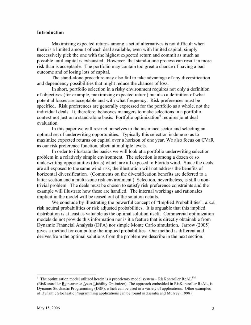
The deals under examination are all exposed to Florida wind events. The

occurrence exceedence curve shown below captures the likelihood of such events.8 Thus in the chart, the likelihood of events greater than $5 billion is shown as 13.9%. Inset in the chart is a calculation of the expected profit ratio from the $5 billion ILW, i.e., premium of 26% less transaction cost equals 23.4% less expected loss of 13.9% gives a profit of 9.5 %. The (net) expected profit ratio is 40.6% (= 9.5%/23.4%).

We will generate scenarios of possible wind events so as to represent the AIR curve. The scenarios will be randomly generated. In the example here 5000 scenarios are drawn and the optimization will take place across that set of scenarios. In practice no

7 Note that in practice participants may have to construct the ILWs with both an industry and indemnity

loss, but that aspect is ignored in this example. 8 We are indebted to AIR Worldwide for this curve.

May 15, 2006 6

sample can fully replicate the original curve, but that is less and less true with bigger

samples9. This provides us with the information to construct the ,i jloss matrix.

In this example, we are provided with a distribution that describes the risky environment. From this, a sample set of scenarios is derived. The minimum size of the

scenario set is: as small as possible or as large as is necessary - so long as it adequately captures the risk environment.

Finally, notice that some clients prefer to generate the scenario set themselves rather than have it generated by the model. In a sense this is what Lloyds of London requires of its syndicates through its “Realistic Disaster Scenarios” [RDS] approach to risk management. It also points the way to another potential application of this approach, since as far as we know Lloyds is monitoring rather than optimizing its franchise value. The model can be run by selected scenarios or by self generated scenarios.

9 As a check on how good the sample is, it is often worth comparing the sample with the original

curve. Another check is to see how stable the solution is against different sample solutions.

May 15, 2006 7

4. Risk Preferences

As we have already asserted, the key to optimization in a risky environment is the risk preference requirements of the portfolio manager. In the example here the constraints, equations (6) for k=1,2,3, are as follows:

1) Probability 30%, CVaR limit of 10% loss of risk capital 2) Probability 20%, CVaR limit of 20% loss of risk capital 3) Probability 0.1%, CVaR limit of 100% loss of risk capital Constraint number 1 means, given all the possible outcomes in the optimal

solutions, that the average loss in the worst 30% of cases must not exceed 10% of risk capital. Constraint number 3 says that the average loss in the worst 1 in one thousand cases must be less than the total capital (i.e. – 100%).

Note that the last constraint does admit the possibility of losses greater than 100% but we know that they will occur with a frequency less than 1 in one thousand (0.1%).

There is often confusion between CVaR and VaR as an expression of risk preference. VaR or “Value at Risk” represents the point on a distribution that divides the outcomes into two frequencies. Typically commercial bankers (and investment bankers) have chosen the frequency as 1 in one hundred (1%). Thus, if the banker knows the 1 in one hundred point, he can require enough capital to cover 99 out of one hundred occasions and feel well provisioned.

This has often been used for daily traded risk positions. Then, every couple of years market extremes will remind bankers that there are many outcomes beyond the 1 in one hundred point. Indeed, the expected outcomes beyond the 1 in one hundred point can be considerably beyond it. The expected value of the outcomes beyond a point is known as CVaR or Conditional Value at Risk. CVaR is superior to VaR in that it does not depend on a single point but rather the average and furthermore it is a “coherent” measure10. That is, it satisfies many of the algebraic qualities that you would want a general “risk measure” to have. VaR does not.

CVaR also has the virtue that it is tractable for portfolio solutions in an optimization framework. In particular, it can be solved in a linear framework11 when the loss function is linear thereby admitting the possibility of very large problems quite efficiently12. And, multiple such constraints can be handled simultaneously, as is done herein.

The distinction between CVaR and VaR is illustrated in the inset panel for a general context. Clearly, users of CVaR for the same frequency as VaR will be more conservative at the same level if they use CVaR to set capital levels instead of VaR because CVaR is always greater than or equal to VaR. In this example, more than one frequency is set to express risk preferences. Management wants to specify the risk of ruin thresholds of course, but they equally likely want to show bad results with some low frequency of occurrence (one year in three or one year in ten, for example) lest shareholders draw the wrong conclusions about their management.

10 See McNeil, Frey and Embrechts (2005). 11 See Uryasev (2000) and Rockafellar and Uryasev (2002). 12 We have solved problems with 50,000 scenarios and around 2,000 complex deals on a workstation in

around 100 minutes with four CVaR constraints plus additional policy constraints.

May 15, 2006 8

There is added motivation to use CVaR in the context of insurance and that is that a lot of risks begin life with probabilities less than 1 in one hundred. A substantial fraction of all the cat bonds issued to date have probabilities less than 1%. Long statistical tails are endemic to insurance. Tail management is what skilled insurance underwriting and CVaR is all about.

Finally, it should be noted that we are not confined to CVaR constraints. We can

also incorporate VaR13, XCVaR, standard deviation, shortfall and many other metrics.14 We feel CVaR is far superior for managing tail risk and for other reasons (discussed in other chapters) because it is a coherent risk measure. (The astute reader of the illustrative panel above will see that VaR, CVaR and shortfall are all inter-related, and it is that which allows accommodation of so many metrics.)

13 It is possible to solve the VaR constrained problem by an iterative application of CVaR constrained

problems. A detailed description of this process is beyond the scope of this paper and will be treated as a

topic in itself in a separate paper. 14 Many of these metrics fly under other banners in other contexts. Thus, expected policy holders deficit

(EPD) is the same as “shortfall”. Lane Financial has used it in Cat bond analysis and called it Conditional Expected Loss (CEL) and in the context of credit derivatives it is the equivalent of Loss given Default

(LGD). Now, the context often provides subtle differences such as there may be an ultimate constraint on

the size of total loss (the size of the bond) but the concepts are essentially the same. CVaR is also known

as TVaR (Tail Var) and XCVaR as XTVaR and so on. There are also subtle differences in these measures

for discrete versus continuous distributions.

Profit and Loss

Probability Distribution

Profitable outcomes - Yellow

Loss outcomes - Red and Cross Hatched

Extreme Losses (1:10) - Red Cross Hatched

0

0.2

-$1,

000

-$90

0

-$80

0

-$70

0

-$60

0

-$50

0

-$40

0

-$30

0

-$20

0

-$10

0 $0

$100

$200

$300

$400

$500

VAR contains 90% of outcomes

CVAR - conditional expected value of

outcomes beyond VAR point

EPD

XCVAR (or XTVAR)

MEAN

This diagram illustrates a distribution of

possible profit and loss outcomes.

The mean (average or expected value)

of outcomes gives a measure of central

tendency.

The other measures are attempts

to capture downside risk. Such measures

are useful for assessing, for example,

capital needs.

VAR is “Value at Risk”. It is that level of Loss

which encapsulates (in this illustration) 90%

of all outcomes. Conversely 10% of the

outcomes will be worse than the VAR level.

When VAR is set at the 99% level some risk -

taking entities have set aside enough capital

to cover 99% of all outcomes.

Experience has resulted in outcomes beyond

VAR and recent risk management has

sought to measure the extent to which losses

will occur beyond VAR. “Conditional Value at

Risk” or CVAR is that measure. It measures

the expected losses given that no more than

10% ( in this illustration) of the losses are

worse than VAR.

“Expected Policyholders Deficit” or EPD is the

expected amount beyond VAR. CEL in other

contexts

NOTE: CVAR = VAR + EPD

ALSO: XCVAR = CVAR +MEAN

- expected amount of penetration

beyond VAR

mean shifted

General

schematic

of

Alternative

Risk

Measures

important

in

Capital

Allocation

Decisions

Profit and Loss





0

0.2

-$1,

000

-$90

0

-$80

0

-$70

0

-$60

0

-$50

0

-$40

0

-$30

0

-$20

0

-$10

0 $0

$100

$200

$300

$400

$500




EPD

XCVAR (or XTVAR)

MEAN





tendency.




capital needs.















worse than VAR.



contexts




beyond VAR

mean shifted

General

schematic

of

Alternative

Risk

Measures

important

in

Capital

Allocation

Decisions

Profit and Loss





0

0.2

-$1,

000

-$90

0

-$80

0

-$70

0

-$60

0

-$50

0

-$40

0

-$30

0

-$20

0

-$10

0 $0

$100

$200

$300

$400

$500




EPD

XCVAR (or XTVAR)

MEAN





tendency.




capital needs.















worse than VAR.



contexts




beyond VAR

mean shifted

General

schematic

of

Alternative

Risk

Measures

important

in

Capital

Allocation

Decisions

Profit and Loss





0

0.2

-$1,

000

-$90

0

-$80

0

-$70

0

-$60

0

-$50

0

-$40

0

-$30

0

-$20

0

-$10

0 $0

$100

$200

$300

$400

$500




EPD

XCVAR (or XTVAR)

MEAN





tendency.




capital needs.















worse than VAR.



contexts




beyond VAR

mean shifted

General

schematic

of

Alternative

Risk

Measures

important

in

Capital

Allocation

Decisions

May 15, 2006 9

5. Other Constraints

It is assumed that only $25 million of limit of each deal is available to write.15 Market size is important to underwriters in practice. Often, deals are syndicated to several reinsurers and writers may not get all that they want. Underwriters may also specify that they do not wish to have more than a certain fraction of a deal. Since we have allowed deals to be written or retroceded we limit the retro possibilities in two ways. First, there is a limit per deal of $5 million (equation (7)). Second, there is a limit of $50 million for the total amount that can be retroceded (equation (5)). Notice that the amount of the deal constraint is expressed in “limit” or “exposure” terms. In other model contexts the limits could be expressed in premium terms. The significance of either specification is that model construction must be bourn in mind when

interpretations of marginal values and other dual values are made.

15 It is important to note that this is not a requirement imposed because we are using a linear programming

model. We will still get finite solutions of the model (in the absence of degeneracy) with no limits because

of the risk constraints.

May 15, 2006 10

6. Stand-Alone Analysis

We asserted that in the absence of capital and/or risk preference constraints, the selection of a portfolio could be done by fairly simple stand-alone textbook rules. To wit, do as much as possible of the deal with the maximum expected profit and continue until a capital limit is reached. The following Table illustrates the procedure.

The deal with the most expected profit is the $5 billion ILW with 9.5% expected

profit per dollar of limit (net of transaction costs). In exchange for assuming $25 million dollars of exposure the reward would be $5.85 million. If, however, an industry loss greater than $5 billion occurred the loss would be $25 million. By writing the 5 deals listed above (in order of decreasing profitability) the accumulated premium would be $18.23 million. Losses, however, could reach $125 million and it would only take one loss of $5 billion to wipe out the premium and put the portfolio in a loss position.

The statistical profile of the stand-alone portfolio is as shown above. Confronted

with this profile the underwriter may well feel that this stand-alone portfolio represents

May 15, 2006 11

too much risk. For example, there is a 13.9% chance of some loss to the portfolio. Further, there is a 3.6% chance of a total loss. This last feature seems extremely high for any institution that wants to stay in business for the long run. Hence, the new constraint 3) above that all of the portfolio outcomes that are worse than the 1 in one hundred point should have an expected loss of no greater than 100%.16 7. The RisKontroller ReAL Graphic User Interface [GUI]

The scenario creation or generation and model solution is a complicated one17. Because we want the process to be used by the reinsurance company as an operational tool, it is necessary to have a suitable user interface. An example of such a user interface is provided by the the RisKontroller ReAL graphical user interface illustrated below. Showing a solution for a simple problem.

A lot of information is concentrated in this optimal solution GUI including the graph of the distribution of returns, the risk report and the balance sheet. Details can be observed by moving the “sliders” in each of the boxes and more information can be displayed in the GUI by “clicking” on the graphs or outputs popup in the Results box.

16 Remember, we are trying to illustrate the general model with a particular example. We are not

suggesting that the model is confined to the structure of this simplified model.

17 We use tools from the Mathworks, see MATLAB web site www.matlab.com, for creating GUIs and

graphics and other numerical procedures and GAMS, see www.gams.com, for the optimization.

May 15, 2006 12

The Optimum Solution

The solution to the simple Florida wind problem is shown in the panels below. It is, on the surface, not too different from the stand-alone solution. Six ILWs are chosen but two of them, the $5 billion ILW and the $20 billion are chosen only to the amount of $6.5 and $6.8 billion, respectively. The other significant difference is the inclusion of the $50 billion ILW. In total, the optimum solution has an exposure of $113.2 million.

The risk profile of the optimum solution is shown below (as an Excel graph). Notice that the graphic shown is the same as the inset graph from the GUI. The only difference is in the method of graphing the discrete points.

May 15, 2006 13

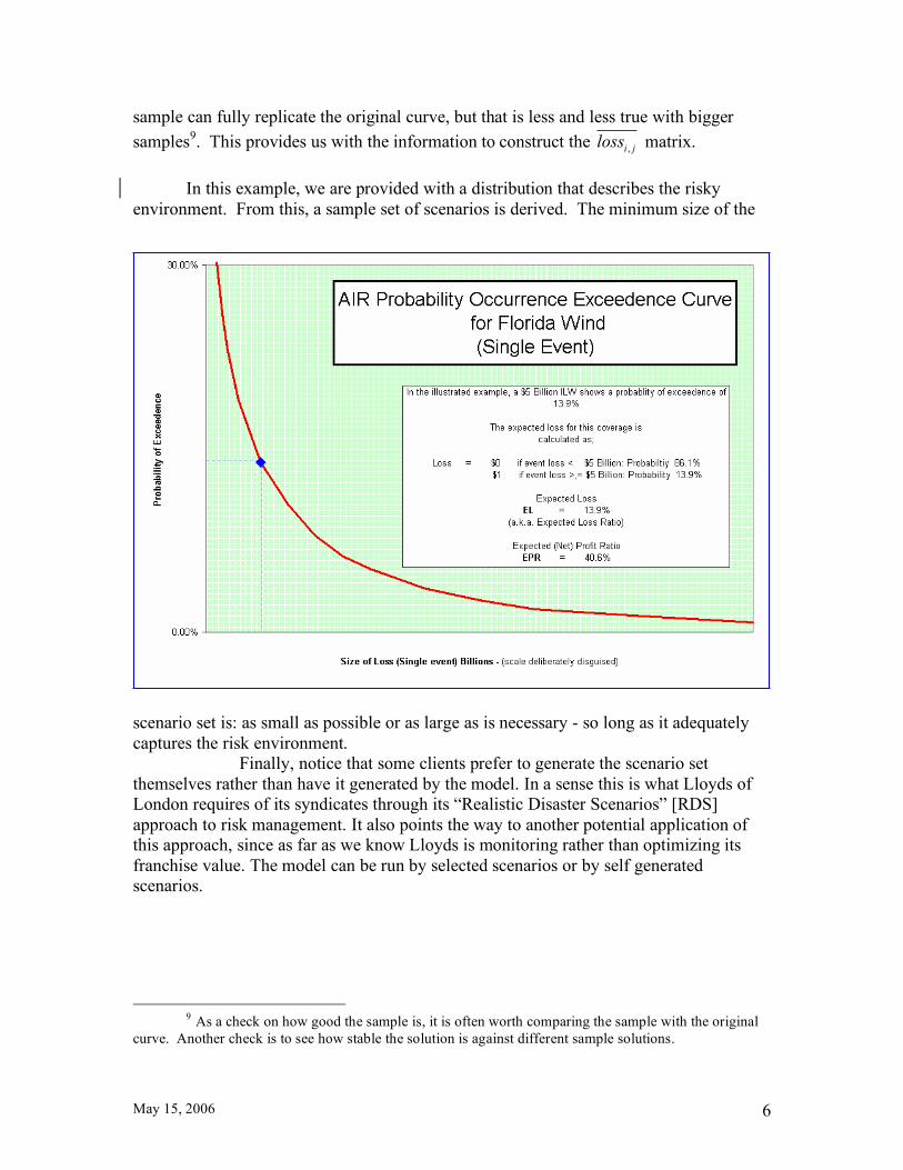
8. The Risk Report

Associated with the optimum solution and its risk profile is the “Risk Report” which contains analysis about how the solution conforms to the risk preference constraints. It is shown below.

At the 30%, 20% and 0.10% frequency level, the CVaR measures are, in terms of the percent of capital, -8.92%, -20% and -100%. In other words, two of the risk preference constraints are “binding”, i.e., they restrict the choice of other solutions that could otherwise increase expected return. The table also shows the VaR level for the 30%, 20% and 0.10% frequency levels. They are, respectively, +13.23%, +13.29% and -100%. Notice the positive return VaR levels. It is intended to demonstrate that while most risk preference is articulated in loss terms, it is equally possible to shape the distribution on the positive side of the curve.

The expected return from the solution is 6.58% return on capital of $100 million. The table shows the source of the returns – written premiums of $14.7 million, none ceded, and expected loss of $6.58 million. Finally, the Risk Report shows two very interesting measures of the marginal value of capital. The first is the marginal value of risk capital – determined to be equal to 5.58%. Conceptually, if the underwriter had another $1 million of capital, how much extra return could be generated by that extra capital? The answer is 5.58%. Clearly, it would be worth acquiring extra capital for less than 5.58%, or, by symmetry, if another alternative use of capital was available returning more than 5.58% it would be worth releasing capital from the optimal portfolio. We use the terms marginal, dual, and reduced cost interchangeably. They all refer to the change

in the objective per unit change in some binding constraint. Mathematically they are usually written as:

(8) f

ub

!=!

May 15, 2006 14

where u is the dual variable, f is the objective function value (expected return in this case), and b

is the value of the right hand side to be perturbed. This assumes differentiability, which need not

be the case in the event of redundancy.

We will be most concerned with the following function v, which in its canonical form is given as:

(9)

( ) min

0

v b c x

Ax b

x

!=

"

"

This function always has a directional derivative and in the direction d, it is given by:

(10) { }( : ) max is optimal in dual problemv b d u d u!" =

where we mean that the maximum is taken over all u that are optimal dual variables in the dual to the primal linear programming problem. These details are discussed in books on linear

programming but we will apply these fundamental results here.

If the dual variables are not unique and this is usually called redundancy because there are more

equations than variables binding at the optimum, the directional derivative does exist and is

defined as above. Whether or not the duals are not unique can be determined precisely in several ways; by actually perturbing the value b and observing the change, by examining a range analysis

given the range of validity of the dual variable, or by noting whether or not duals with zero values

are associated with active constraints.

In lieu of one of these procedures, the duals produced from a linear program should be thought of

as identifying suspects and we use them in the following as if that were true. We explore the

other case elsewhere.

We use this approach to determine the marginal risk adjusted return on capital. Attached to each

equation or inequality is the definition of a dual variable. The values of dual variables are given as a part of an optimal solution. If the right-hand side of an equation is itself a function of

another variable then we can define the following:

(11)

where ( )

f f b

b

b b

! !

!

" " "=

" " "

=

Now, we will replace the variable capital by capital !+ everywhere in the model equations

where we take ! to be a perturbation in the amount of capital. Then we can apply the above and

we have a formula for the marginal return on the rate on equity per unit of capital as:

(12) (1 ) ki k k

i k

frate u tm ucap c cvar ucvar

!

"= + # + $ #

"% %

May 15, 2006 15

where ucap is the dual to equation (5), iu are the duals to equations (3), and

kucvar are the

duals to the k CVaR constraints. Why, one might ask, is the expected marginal use of capital 5.58% if the portfolio expects to return 6.58%? One answer is that we are changing a single variable – capital – not scaling all restrictions, so the marginal value of capital will reduce the more of it there is, all else being equal. A second answer is that the quantity of capital restricts the optimum solution through its effect on the CVaR, i.e., risk preference constraints. Two of these are binding. Adding extra capital releases the pressure of these constraints. And one can deduce from the respective dual values that the 3rd constraint, i.e., the 1-in-one-thousand constraint, is the “most binding”. Its value is 25.11 vs. 0.77 on the 2nd constraint and zero on the 1st constraint. So, one might expect that the actual marginal is some weighted average of these. A third reason is that the portfolio return is the total return whereas the marginal return on capital holds only at the limit. There is another concept of marginal return, the marginal value of non-risk capital that is quantified in the risk report. Its value is 17.87%. If the underwriter had an extra $1 million of cash which was not subject to the CVaR constraints, he could generate an expected $0.1787 million, i.e., 17.87%. What extra cash could that be? Possibly it could be extra premium, possibly retrocessional capital, possibly return from operational cost savings. In any case, generally, it is the return from internally generated capital.

A second part of the risk report is the full detailing (above) of VaR and CVaR at different levels of frequency. Notice in this solution that the traditional 1% level shows that the VaR of the optimum solution is -75%. The CVaR at 1% is -97%.

May 15, 2006 16

9. Balance Sheet and Income Statement

Although this example is a simple one it is worth reporting the optimum portfolio in pro forma expected Balance Sheet and Income Statements, thus:

Gross written premium is $14.70 million, none is ceded and expected losses are $6.65 million. That amount less acquisition expenses of $1.47 million (i.e. the 10% transaction costs) gives an expected profit of $6.58 million. Total exposure is $113.23 million so the leverage is 1:1.13. Underwriting profit is $8.06 million. The Expected Loss Ratio of the optimum portfolio is 45.2%.

May 15, 2006 17

10. Deal by Deal Marginal Reports

Beyond the optimal solution and its financial consequences, an optimizing model can provide much additional information about marginal values.18 To some extent that is obvious from the Risk Report. However, much more information can be gleaned from the dual of the optimum solution. It is something that optimization can do that is NOT available from a simulation model.

The blue shaded table shows the deal by deal marginal analysis (the dual variables to the constraints (7)). The yellow shaded table shows the input table for reference. Now, the $10 billion ILW is part of the optimal solution and was written at a (gross) price of 17.5% rate on line. It was written to the limit of $25 million. Two questions are possible with marginal analysis: how low could the price drop before it ceased to be attractive, and if an additional $1 million of limit was available what would it be worth? The table shows that the price of the ILW could drop to 16.13% before it ceased to be attractive. Similarly, the $12.5 billion and $15 billion ILWs could drop to 13.31% and 11.82%, respectively. In contrast, the $30 billion ILW is not part of the solution at a price of 5.80%. Its price would have to rise to 6.19% to be included in the solution. The answer to the second question, what is the value of an extra $1 million of limit, is shown in the marginal column. An extra million of limit for the $10 billion ILW is 1.24%. Similar questions exist for the retrocessional opportunities. In the table below the $10 billion ILW, which could be written all the way down to 16.13%, would become attractive to retrocede if the price were to drop as low as 12.62%. Notice also that all the marginals are negative, indicating that none of the opportunities are good for being ceded.

18 The issue of non-unique marginal values, when they occur, can be handled using directional derivatives.

May 15, 2006 18

11. Deal Ranking

The marginal values attributed to each deal can be used to rank the deals from best to worst expected returns. See table below.

Clearly, the most valuable transaction on a marginal basis is the $12.5 billion ILW. It and the rank ordering of deals in the table are quite different from the stand-alone analysis rankings.

Later it will be apparent that there are other ways to rank the transactions using implied probabilities directly. And it can be proven that the deal acceptance/rejection criteria using only implieds directly are identical to the use of marginals. This is because using the marginals includes the marginal effect on all constraints that are affected. Using implieds only considers the effect on scenarios. The relationship between the two is proportionate – hence the same rank ordering.

May 15, 2006 19

12. Implied Probabilities

19 - How the Risk Adjustment Process Works

The scenario set that is generated from the specified distribution, or is independently supplied by the client, is randomly drawn. Each scenario has equal weight although the concentration of scenarios at each point on the scale of possible outcomes will represent the probabilities of the source distribution. Each of these scenarios has a different effect on each of the deals being considered and a vector of outcomes is generated for the behavior of each deal in the scenario set. Because of this, some deals will have greater or lesser impact on each of the constraints, in particular on each of the CVaR constraints. The optimizing model weighs up the relative contributions of each deal and trades them off to maximize expected return subject to those constraints. In effect, the model weights the scenarios with different weights and these can be turned into a probability equivalent distribution of outcomes. Sections of the table of the implied probability set are shown below.

For scenario ID number 11 there is a wind event that is assumed to cause an industry loss of $12.73 billion. There is no loss for scenario IDs 1, 2, 3 and 4 nor 6, 7, 8, etc. There may be a loss for each of the 5000 scenarios. Equally weighted, the probabilities are 1/5000 = 0.0002 as in column 2. In contrast, column 3 shows the implied probabilities. Implied by what? Implied by the optimal solution and the various trade-offs necessary to that solution. Thus, scenario ID number 1 has an implied probability of 0.0003, as do all of the first 15 scenarios. Other sections of the full report, however, show different probabilities. For

19 The issue of implied probabilities and incomplete markets is discussed in a later paper. These implied

probabilities are similar to the Arrow-Debreu prices or state-price deflators in options theory.

May 15, 2006 20

example, scenario 214 (an industry loss of $55.2 billion) has an implied probability of 0.00456 and scenario 4707 (zero industry loss) has a probability of .00017. The implied probabilities are obtained from the duals of equation (3) where we let

( )1 2, ,...,

nu u u u= . It can be shown that if we define

uu

e u=

! where ( )1,1,...,1e = , then

u satisfies several interesting properties. First, the iu sum to one and therefore can be

considered probabilities. They can be used to price a deal with a loss vector

( )1 2, ,...,

nL l l l= in the following way:

(13)

{ }

0

1 1

1 1

where

and 1+ 1

uprice E L

r trs

uu

e u

ur ratee u

! "! "= # $# $

+ %& '& '

=(

= = +(

Here, uE is the expectation operator in the probabilities u ,

0u is the dual to equation (2),

and rate is the rate of return on internal capital or the risk-free rate. The price is the

arbitrage free price. The price equation (13) looks like that of the Arrow-Debreu model of the securities market. A simplified version of our model does indeed reduce precisely

to that case. The duals iu then will be shown to correspond to “risk-neutral probabilities”

and can be used to compute “state-price deflators20.” We used 0rate = in our Florida

example. For the simple case where we already have a price in our model, we can compute the arbitrage free price either by (13) or by the following price change:

(14) 0

1 1

1 1

ubdprice

r utrs

! "! "# = $ %$ %

+ &' (' (

The effect of the implied probabilities is to describe a different distribution. It is shown in the diagram above and is contrasted with the sampled scenario set. The graph shows exceedence curves.

20 See Avellaneda and Laurence (2000).

May 15, 2006 21

Clearly, the implied curve is more conservative than the actual curve. In the point referenced, the $20 billion ILW, AIR says that the probability of an event exceeding $20 billion is 4.26%. However, the model says, given the opportunity set and the specified risk preferences, one ought to view that as an 8.52% probability. If you don’t assume this conservative probability you are not adequately making a risk adjustment for the desired preferences. Risk adjustment is a much used phrase, but is a much underused mathematical process. Only in the context of the capital market pricing model is there an explicit attempt to risk-adjust prices (by some fraction of the standard deviation, a la William Sharpe’s suggestions) or variations thereof (like the “Risk Ratio”, the “Efficiency Ratio” or ratios that use CVaR or VaR in the denominator instead of standard deviation like RAPM). Beyond that, it is usually a mantra of faith. Using the phrase risk-adjusted is a

calculated reference to good practice rather than a practice of good calculation.

In the case of optimization models, there is implicitly both good practice and good calculation. And as we shall see, once understood it is extremely powerful information.

May 15, 2006 22

13. Risk Adjusted Returns

For each deal under consideration it is possible to work out a vector of outcomes for each of the 5000 scenarios as seen in equation (3). The expected value of the deal is the average of all these outcomes. Then given premium, less transaction costs and the expected loss, it is possible to assign an expected profit to each deal. We refer to this as an “a priori expected profit”. It is prior to any risk adjustment. Now that we have a second distribution – the implied distribution – which is risk adjusted, we can do exactly the same calculation to arrive at a “risk adjusted expected profit” as per equation (13). Both numbers are listed for each deal in the table below.

There are two features to notice in this table. First, the risk adjusted numbers are much lower than the a priori numbers. Second, the rank ordering of the a priori numbers is different from the risk adjusted numbers. The best deal on an a priori basis is the $5 billion ILW, but on a risk adjusted basis the best deal is the $12.5 billion ILW. Notice another feature, alluded to in an earlier section. The rank ordering by implied probability is the same as it is by marginal. Also, examining the deals accepted vs. those rejected it is clear that the process is “accept if risk adjusted expected returns (or marginals) are positive, and reject if negative” – see table below.

May 15, 2006 23

Another way to view the a priori vs. risk adjusted returns comparison is graphically. Thus, in the diagram below the axes represent the different measures. It is clear that the $5 billion ILW is rated quite high on an a priori basis but is strictly marginal when viewed on a risk adjusted basis.

May 15, 2006 24

14. Stand-Alone vs. Optimum Solution

At the outset of this description we said that choosing a good portfolio was not difficult as long as one didn’t have any capital or risk preference constraints. Portfolio selection could be done on a stand-alone basis. However, as long as management was concerned with avoiding devastating outcomes, or at the very least reducing the frequency of their occurrence to a minimum, portfolio selection has to be done in an integrated context. The results are shown in the graphic and inset tables below.

There is a trade-off between higher expected return, 9.08%, in the stand-alone solution vs. the risk it assumes. When risks are confined to what is acceptable the expected return is reduced to 6.58% but, hopefully, survival of the entity is more assured and consistent with underwriter desires.

May 15, 2006 25

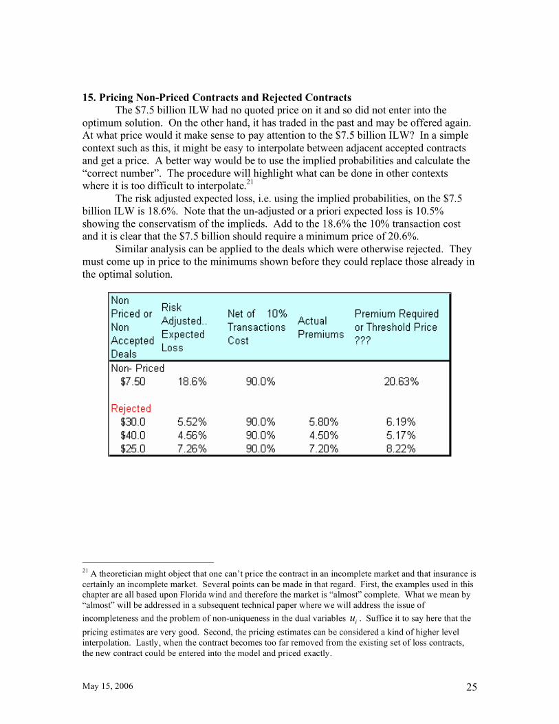
15. Pricing Non-Priced Contracts and Rejected Contracts

The $7.5 billion ILW had no quoted price on it and so did not enter into the optimum solution. On the other hand, it has traded in the past and may be offered again. At what price would it make sense to pay attention to the $7.5 billion ILW? In a simple context such as this, it might be easy to interpolate between adjacent accepted contracts and get a price. A better way would be to use the implied probabilities and calculate the “correct number”. The procedure will highlight what can be done in other contexts where it is too difficult to interpolate.21 The risk adjusted expected loss, i.e. using the implied probabilities, on the $7.5 billion ILW is 18.6%. Note that the un-adjusted or a priori expected loss is 10.5% showing the conservatism of the implieds. Add to the 18.6% the 10% transaction cost and it is clear that the $7.5 billion should require a minimum price of 20.6%. Similar analysis can be applied to the deals which were otherwise rejected. They must come up in price to the minimums shown before they could replace those already in the optimal solution.

21 A theoretician might object that one can’t price the contract in an incomplete market and that insurance is

certainly an incomplete market. Several points can be made in that regard. First, the examples used in this chapter are all based upon Florida wind and therefore the market is “almost” complete. What we mean by

“almost” will be addressed in a subsequent technical paper where we will address the issue of

incompleteness and the problem of non-uniqueness in the dual variables iu . Suffice it to say here that the

pricing estimates are very good. Second, the pricing estimates can be considered a kind of higher level

interpolation. Lastly, when the contract becomes too far removed from the existing set of loss contracts,

the new contract could be entered into the model and priced exactly.

May 15, 2006 26

16. Pricing an Excess of Loss Contract (XoL)

Only ILWs were part of the original eligible set of opportunities. But that does not mean that the underwriter flies blind in evaluating other structures, considered after the portfolio was optimized. Once again the key is to price the structures using the implied probability distribution. Below, two excess of loss deals – a specified % of $10 billion XS $10 billion and a % of $10 billion XS $20 Billion – are evaluated. As the inset panels show, they must be priced at minimums of 12.18% and 7.82% to be attractive.

May 15, 2006 27

17. Pricing Retro Contracts

There are many different forms of retrocessional coverage that can be purchased by an underwriter. Simply using the ILW market is one method that links recoveries to industry losses. Another form is to link retrocessional recoveries to company, or in this case portfolio, losses. This, of course, is indemnity coverage. Yet other retrocessional forms link recoveries to company losses (indemnity) but are contingent upon industry event losses. Each of these can be evaluated using implied probabilities to establish when it makes sense to retrocede. In the example below we explore the value of indemnity retrocessional coverage for $25 million XS $25 million. The risk adjusted expected value of the contract, i.e., using implied probabilities as a % of limit, is 11.83%. Now we are purchasing the coverage and so don’t want to pay more than 11.83% in total since part of this is transaction cost. The stated price to make it worthwhile to buy this retro is 10.75%.

Just to reinforce the point about threshold levels, such as the 10.75% derived for a potential $25 million XS $25 million cover, remember that a purchase at that level would not improve portfolio expected returns. It may reshape the risk profile but not enhance return. However, if the same cover could be purchased at a rate on line of 9% we could anticipate an expected incremental return of 1.75% (10.75%-9%).

Retrocessional purchases on a stand-alone basis are always negative present value deals, because premium outlays are in excess of expected recoveries. On a risk adjusted basis, however, retrocessional purchases can be beneficial. They will always be so if the risk adjusted price of the retro is below the risk adjusted threshold.

In practice, RisKontroller ReAL can be designed to provide a set of threshold retro prices for each of several common forms of retro – ILW, industry excess of loss, indemnity excess of loss, or contingent, at each point on the designated loss scale. It can be used to direct management where to buy retro to best complement the optimal solution.

May 15, 2006 28

19. Conclusions

This paper has drawn out the virtues of using optimization techniques for

selecting underwriting portfolios. Further, it has illustrated that beyond the primal solution, the dual solution provides extremely valuable economic information for the underwriter. The value of dual information has long been known in optimization models, but to our knowledge is mostly used in deterministic environments. Utilization of dual values in a stochastic environment is relatively rare. It requires some heavy algebra, but we believe it is worth the effort. Hopefully that has we demonstrated. To review, our solution has provided the following;

• Optimal allocation to deals • Marginal Value of additional risk capital • Marginal value of additional non-risk capital • CVaR and VaR profiles to the optimal solution • Marginal values of risk preference constraints • Marginal value of each deal • Rank ordering of deals • Implied Probabilities consistent with specified opportunity set and

preferences This set of implied probabilities is vitally important for further analysis. In this example we have shown that they can be used to gage the value of marginal additions to the portfolio of contracts not initially specified in the model. Examples have been provided of evaluating marginal additions of excess of loss contracts and retrocessional opportunities. Simultaneous solution of a set of traditional underwritings opportunities and retrocessional alternatives is highly non-linear and difficult to solve. Here however we have shown a way of iterating to a solution. Furthermore we have illustrated why retrocession can have a positive value on a risk adjusted basis despite it usually being a negative activity on an a priori basis. Of course the environment in which we have illustrated these undoubted virtues is fairly primitive – a single risk zone – in our example, Florida Wind. That is not the only environment that we have deployed the procedure. Two other contexts are; for a hedge fund transacting in multiple risk zones with simple ILWs and Cat bonds, and in a real reinsurance company.

In the hedge fund context the trade off between various layers of risk and various zones of risk are made explicit. The model picks up the various correlations implicit in contract selection by generating scenarios over all zones. For example, California earthquake and Florida Wind are uncorrelated but contracts that cover both perils, for example US All Natural Perils ILWs will have an implicit correlations with Florida Wind and US Earthquake. The scenarios generated pick up that correlation and the optimization selects so as to achieve over all portfolio objectives and risk preferences. The implied probabilities can even be used to provide measures of “correlations to the portfolio” for contracts considered both within and outside the opportunity set. It can also be used to evaluate whether new lines of business should be added to the solution and how much is their risk adjusted contribution or value.

May 15, 2006 29

In the application to a real reinsurer large size problems have been solved with outputs just as valuable in the simple case laid out here. Typically these applications are solved with a 1,500 deal opportunity set and 40,000 to 50,000 scenarios. There is no reason why one million or more scenarios can not be used in the optimization. In such large problems for large companies often the underwriting is done in different departments as well as different countries. One classic management problem this causes is how to make the departmental underwriting solution consistent with the company wide objectives. When authority is delegated, how does one ensure the delegated solutions contribute to the global optimum and not be sub-optimal? It turns out that the implied probability set gives each independent underwriter the correct signal to contribute to the global optimum. This is potentially extremely valuable. So too is the capital allocation information that the solution brings. But that is for another paper.

Another problem of insurers is the interplay between the asset and liability sides of the balance sheets. In our example we assumed fixed investment returns. If they were stochastic investment returns the risk preference set would suggest a slightly different optimum portfolio. That is important. What one underwrites is not independent of what one invests in, and vice versa. One may guess that the marginal value of non-risk capital will figure in the asset, liability risk trade-off.

Many of the classic problems of capital allocation and delegation of underwriting authority are not new to insurers. They live with them every day. What is new here, with optimization, is the ability to answer the question in a holistic, consistent, quantitative manner that does not rely on trial and error or the instincts of experienced underwriters. Further more decisions can be made which are consistent with the articulated risk preferences of management, shareholders, ratings agencies and other stake holders.

May 15, 2006 30

References

Avellaneda, Marco and Peter Laurence. 2000. Quantitative Modeling of Derivative Securities,

From Theory to Practice, Chapman and Hall, Boca Raton.

Birge, John R. and Francois Louveaux, 1997. Introduction to Stochastic Programming, Springer

Series in Operations Research, Springer, New York.

Claessens, Stijn and Jerome Kreuser. 2004. “A Framework for Strategic Foreign Reserves Risk

Management,” in Risk Management for Central Bank Foreign Reserves, European

Central Bank Publication, Frankfurt am Main, May.

Christensen, Claus Vorm. 2000 Implied Loss Distributions for Catastrophe Insurance

Derivatives. working paper, Laboratory of Acturial Mathematics, University of

Copenhagen (Available at: http//www.imf.au.dk/~vorm)

Jarrow, Robert A. 2005. “Valutaion of Insurance Contracts in Incomplete Markets”, Prelimianry

Paper, Cornell University, April 25.

Jorion, Philippe. 2000. Value at Risk, Second Edition, McGraw-Hill.

Lane Morton N. (Ed) 2002 Alternative Risk Strategies, Risk Books

Lane, Morton and Jerome Kreuser. 1980. "Designing Investment Strategies for Fixed-Income

Portfolios," in Extremal Methods and Systems Analysis, Ed. A.V. Fiacco and K. O. Kortanek,

Springer-Verlag, New York.

Lane Morton and O. Y. Movchan. 1998 The Perfume of the Premium II Sedgwick Lane

Financial Trade Notes (Available at: http//www. lanefiancialllc.com)

McNeil, Alexander J., Rüdiger Frey and Paul Embrechts, Quantitative Risk Management,

Princeton University Press, 2005.

Rockafellar, R. Tyrrell and Stanislav Uryasev. 2002. “Conditional Value-at-Risk for General

Loss Distributions,” in the Journal of Banking and Finance, Vol. 26(7), July.

May 15, 2006 31

Uryasev, Stanislav. 2000. "Conditional Value-at-Risk: Optimization Algorithms and

Applications," Financial Engineering News, Issue, February

Ziemba, William T. and John M. Mulvey. 1998, Worldwide Asset and Liability Modeling,

Cambridge University Press, UK

May 15, 2006 33

an introduction to the benefits of optimization models for · an introduction to the benefits of...

Documents