an introduction to the extended finite element method (x-fem)
TRANSCRIPT

Extended Finite Elements
An introduction to the eXtendedFinite Element Method (X-FEM)

2
Extended Finite Elements
Eric Béchet (it's me !)
Engineering studies in Nancy (Fr.)
Ph.D. in Montréal (Can.)
Academic career in Nantes, then Metz (Fr.)
Then Liège... Contact : [email protected]

3
Extended Finite Elements
Lecture plan
Introduction Reminder Simple problems (jump on the primal variable) Extensions in 2D / 3D Other types of problems (jump on the
derivatives) Other applications and current research Boundary conditions References

4
Extended Finite Elements
Course Notes available at :
http://www.cgeo.ulg.ac.be/X-FEM

5
Extended Finite Elements
Introduction
“Classical” finite element computation The geometry is bounded by element sides
Bounds the computation domain Bounds the interface between zones of dissimilar
properties A change in geometry implies a
change in the mesh Time evolving problems
may induce remeshingat each time step in thecomputation

6
Extended Finite Elements
Introduction
Mesh generation techniques May be costlier than the sole finite element
computation (Often) necessitates a strong human interaction Are a potential source of mistakes
Of human origin Or from the lack of robustness of remeshing algorithms

7
Extended Finite Elements
Introduction

8
Extended Finite Elements
Introduction
The idea here: Minimize the constraints on the mesh that is used in
the FEM simulations However, mesh generations is still necessary
e.g. the accuracy of the computation depents on the quality of the mesh
→ mesh adaptation

9
Extended Finite Elements
Reminder
We will realy on the classical FEM; starting with the weak form of a physical problem :
Discretization: One look for u in a discrete function space (trial functions v belong to the same space )
uh x =∑i
i N i x , x∈
Find u∈H 1(Ω) such that
∫Ω
a(u , v)d Ω=∫Ω
b(v)d Ω ∀ v∈H 01(Ω)
V h⊂H 1(Ω)
V 0h⊂H 01(Ω)

10
Extended Finite Elements
Reminder
A space-conforming mesh is used to define the shape functions SFs
Thay have a compact support Partition of unity Interpolation
∑i
N i=1
u x i=i
u(x)=∑k
λ k N k for x∈T j

11
Extended Finite Elements
Reminder
SFs with a compact support Allows to have banded matrices (low memory
imprint) Partition of unity
One is able to represent a constant field ! Interpolation
Easy to impose Dirichlet boundary conditions Use of conforming meshes
Pre-computations of many operators is possible at an elementary level

12
Extended Finite Elements
Simple problem
Clamped 1D Bar (L, E, S) with a variable load f(x)
One wants to get the displacement u(x) and assume that the bar is cut at some place
With the classical FEM With the eXtended Finite Element Method
f(x)
L

13
Extended Finite Elements
Simple problem
Weak form, with homog. boundary conditions
with Elementary (stiffness) matrix
Elementary vector (loads)

14
Extended Finite Elements
Simple problem
Discretization : Linear elements, nodal shape functions.
uh x =∑i
i N i x
N 1 x N 2 x N 3 x N 4 x

15
Extended Finite Elements
Simple problem
By reporting the discrete form of u and v in the weak form, one gets the following linear system :
Here, coefficients and vanish (clamped extremities)
[k 22 k 23
k 32 k 33]⋅2
3= f 2
f 3
1 4
k ij=∫0
L
ES∂ N i
∂ x⋅∂ N j
∂ xdx
f i=∫0
L
N i⋅ f x dx

16
Extended Finite Elements
Cut the bar : FEM case
Add two nodes and do the same This is called « remeshing », it is simple, fast and
robust in 1D, less 2D and much less in 3D
N 1 x N 2 x N 3 x N 4 x
N 5 x N 6 x

17
Extended Finite Elements
Cut the bar : FEM case
After discretizing, one gets :
The two circled parts are independent One could solve the linear system separately for
each sub-problem
[k 22 k 23 0 0k 32 k 33 0 00 0 k 44 k 45
0 0 k 54 k 55]⋅
2
3
4
5=
f 2
f 3
f 4
f 5

18
Extended Finite Elements
Cut the bar : FEM case
The meaning of the DoFs is kept ( means the displacement of node i.)
There is indeed a discontinuity in the displacement at nodes 3 and 4
Nothing changes in the implementation – only the mesh and its topology are modified
i

19
Extended Finite Elements
Cut the bar : X-FEM case
Now : we don’t change the mesh ! But one can add/modify shape functions
N 1 x N 2 x N 3 x N 4 x

20
Extended Finite Elements
Cut the bar : X-FEM case (I)
Case (I) :
N 1 x N 3+ x N 4 x N 2
- x

21
Extended Finite Elements
Cut the bar : X-FEM case (I)
Case (I) :
N 1 x N 3+ x N 4 x
+N 2
+ x
N 2- x

22
Extended Finite Elements
Cut the bar : X-FEM case (I)
Case (I) :
N 1 x N 3+ x N 4 x
+N 2
+ x
N 3- x
+
N 2- x

23
Extended Finite Elements
Cut the bar : X-FEM case (I)
How to compute the from the ? Let’s introduce the Heaviside function :
This is its complement :
s is the distance to the cut (here, )
N j+,- N i
H (s)={0 if s≤01 if s>0
H (s)={1 if s≤00 if s>0
s=x−L2
24
Extended Finite Elements
Cut the bar : X-FEM case (I)
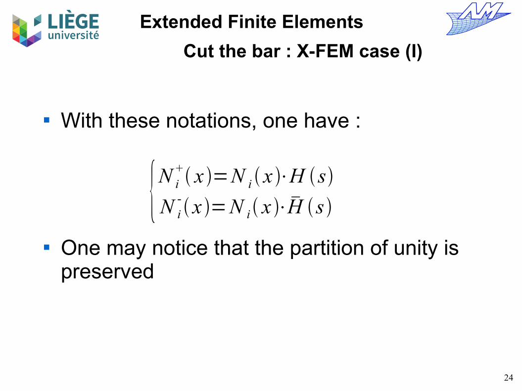
With these notations, one have :
One may notice that the partition of unity is preserved
{N i+ x =N i x ⋅H s
N i- x =N i x ⋅H s

25
Extended Finite Elements
Cut the bar : X-FEM case (I)
One has to sort the mesh nodes Those which have “regular” degrees of freedom
go into set N Those which have modified degrees of freedom
go into set C The solution field u is written as :
u x =∑i∈N
i N i x ∑j∈C
j+ N j
+ x ∑
k ∈C
k- N k
- x

26
Extended Finite Elements
Cut the bar : X-FEM case (I)
Linear system We number the DoFs as follows :
[ 1 2 3 4 5 61 2
-3
-2
+3
+4
]
[k 22
- k 23- 0 0
k 32- k 33
- 0 0
0 0 k 22+ k 23
+
0 0 k 32+ k 33
+ ]⋅2
-
3-
2+
3+=
f 2-
f 3-
f 2+
f 3+

27
Extended Finite Elements
Cut the bar : X-FEM case (I)
Again, we manage to separate the domain in two parts
The signification of the degrees of freedom is partly lost
Some shape functions have to be modified Two “Heaviside” functions are needed to
modify the shape functions

28
Extended Finite Elements
Cut the bar : X-FEM case (II)
Without changing the shape functions ! (case II)
N 1 x N 3 x N 4 x
+
N 2* x
N 3* x +
N 2 x

29
Extended Finite Elements
Cut the bar : X-FEM case (II)
How to compute the from the ? Lets introduce the modified Heaviside function :
With this notation, one finds that :
N j* N i
H *(s)=2 H (s)−1={−1 si s≤0
1 si s>0
N i*x =N i x ⋅H *
s

30
Extended Finite Elements
Cut the bar : X-FEM case (II)
One should again sort the mesh nodes Those which have modified DoFs go into set C “regular” shape functions are still everywhere (no
change with regular FEM in that case) The solution field u is written as :
u x =∑i∈
i N i x ∑j∈C
j* N j
* x

31
Extended Finite Elements
Cut the bar : X-FEM case (II)
Linear system We number the DoFs as follows :
[ 1 2 3 4 5 61 2 2
*3 3
*4
]
[k 22 k 22* k 23 k 23*
k 2*2 k 2* 2* k 2*3 k 2* 3*
k 32 k 32* k 33 k 33*
k 3* 2 k 3* 2* k 3*3 k 3*3*
]⋅2
2*
3
3*=
f 2
f 2*
f 3
f 3*

32
Extended Finite Elements
Cut the bar : X-FEM case (II)
At the matrix level, the two parts are linked Are there two physically separated parts ?
Lets assemble the matrix without taking care of the boundary conditions, and then determine the number of vanishing (singular) eigenvalues of this matrix.
If there is only one entity, there will be only one singular eigenvalue (corresponding to the missing Dirichlet BC to get a non singular system)
Two singular values → the bar is indeed cut in two, and two Dirichlet boundary conditions are needed.

33
Extended Finite Elements
Cut the bar : X-FEM case (II)
Case without cut and without BC : typical matrix
det K s− I =0
K s=k⋅[
1 −1 0 0−1 2 −1 00 −1 2 −10 0 −1 1
]
One eigenvalue vanishes.
k=3ES
L

34
Extended Finite Elements
Cut the bar : X-FEM case (II)
Case with a cut and without BC : typical matrix
K c=k⋅[
1 −1 1 0 0 0−1 2 −1 −1 0 01 −1 2 0 −1 00 −1 0 2 1 −10 0 −1 1 2 −10 0 0 −1 −1 1
]Two eigenvalues vanished : it is OK
det K c− I =0
35
Extended Finite Elements
Cut the bar : X-FEM case (II)
The meaning of the degrees of freedom is lost
One keeps classical FE basis functions and add others by enrichment
A kind of hierachical FE basis is built Only one enrichment function (simpler !)

36
Extended Finite Elements
Cut the bar : X-FEM case
Cases (I) and (II) are equivalent (the results are exactly identical)
We ideed have a linear combination between shape functions of (I) and those of (II) :
The case (II) is part of the more theoretical frame – use of a given enrichment function and “constructive” synthesis.
N 2 x =N 2+ x N 2
- x
N 2* x =N 2
+ x −N 2
- x
N 3 x =N 3+ x N 3
- x
N 3* x =N 3
+ x −N 3
- x

37
Extended Finite Elements
Definition
eXtended Finite Element Method It is based on classical FEM basis functions The product between these functions and a given
enrichment function is then added These enriched fnctions are able to represent a
specific behavior of the solution field that classical shape functions are unable to represent efficiently. (e.g. a discontinuity)
u x =∑i∈
i N i x ∑k∑j∈C
jk* N j x ⋅E k x
E k x

38
Extended Finite Elements
Lecture plan
Introduction Reminder Simple problems (jump on the primal variable) Extensions in 2D / 3D Other types of problems (jump on the
derivatives) Other applications and current research Boundary conditions References

39
Extended Finite Elements
In 2D / 3D
Case of linear elasticity Representation of cracks Level-sets Crack propagation

40
Extended Finite Elements
2D Example
A wedge with constraineddisplacements (linear elast. )
a u ,v =∫
∇su : D: ∇
sv d
bv =∫
f⋅v d
find u such thata(u , v)=b( v) ∀ v

41
Extended Finite Elements
2D Example
Displacements without cut (standard FEM)
u x =∑ i⋅ N i x
N i x The are the classical linear shape functions (order 1 Lagrange)

42
Extended Finite Elements
2D Example
Lets impose a cut path Modifications of the function
space :
How to define
and the set C ?
u x =∑i∈
i⋅ N i x
∑i∈C
i*⋅ N i x ⋅H *
s
H *s

43
Extended Finite Elements
2D Example
lsn x
s=lsn x
H *s=H *
lsn x
={x∈ℝ3/ lsn x =0}
lsn x
The cutting path may be defined with a “level-set”We have
is the signed distancefunction (to the interface)
One simply takes :

44
Extended Finite Elements
2D Example
Definition of the enriched degrees of freedom (the set C)
Those are the nodes of the elements completely cut by (iso-0 of the level-set )

45
Extended Finite Elements
2D Example
After assembly and solvingthe linear system one getstwo independent solids(as expected)
The geometry of may be arbitrary.
No need of anyremeshing

46
Extended Finite Elements
Integration issues
Integration One need to subdivide elements that are cut by the
interface (discontinuous functions to integrate) On each sub triangle (in red here), a classical Gaussian
quadrature is used because the integrand is a polynomial.

47
Extended Finite Elements
Cracks
Crack modeling Historically, this is the first application of the
extended finite element method The crack propagates, and one does not want to
generate a new mesh at each time step A crack is in fact an incomplete
cutting in the domain

48
Extended Finite Elements
Cracks
Geometrical representation of the crack It is not part of the mesh (by definition) Its surface is therefore defined, as before, with a
level set lsn that represents the normal distance to the surface.
One also needs the location where it stops (on its surface)
Crack tip (or front in 3D )

49
Extended Finite Elements
Cracks
lst x
We make use of another level set
It represents the distance to thecrack front(measured tangentially)
Both level sets forman orthogonal basisat the crack tip

50
Extended Finite Elements
Cracks
={x∈ℝ3/ lsn x =0, lst x ≤0 }
The locus of the crack is therefore defined as :
The enrichment set C is also modified :

51
Extended Finite Elements
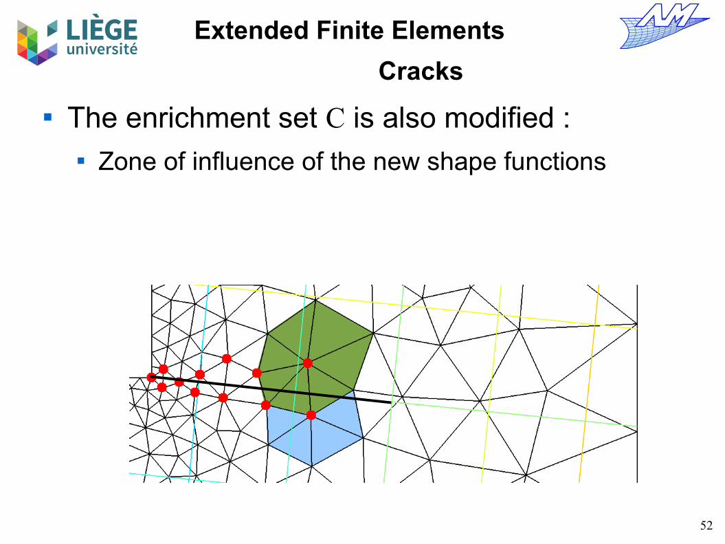
Cracks
The enrichment set C is also modified : Zone of influence of the new shape functions
52
Extended Finite Elements
Cracks
The enrichment set C is also modified : Zone of influence of the new shape functions

53
Extended Finite Elements
Cracks
The enrichment set C is also modified : Zone of influence of the new shape functions
Either it cannot cover the crack until its tip or front...

54
Extended Finite Elements
Cracks
The enrichment set C is also modified : Zone of influence of the new shape functions
Either it cannot cover the crack until its tip or front...
or it goes a bit too far

55
Extended Finite Elements
Cracks
A special procedure is needed at the crack tip The enrichment function should be discontinuous
until the crack tip; continuous beyond.

56
Extended Finite Elements
Cracks
T (s , t )={0 if t≥0H *
(s) if t≤−e
−t H *(s)
e if −e<t<0
with {s=lsn(x)t=lst (x)
e
t
s
e could be some elements wide

57
Extended Finite Elements
Cracks
Alternate set of enriched elements C' It includes every node for which the support is cut
(at least partly) by the crack.
u x =∑i∈
i⋅N i x ∑i∈C'
i*⋅ N i x ⋅T t , s

58
Extended Finite Elements
Cracks
Displacements with acrack tip enrichment

59
Extended Finite Elements
Cracks
In fact, the form of the exact solution is known at the crack tip
Why not use this directly as a crack enrichment function ?
It is readily available for a crack in an infinite medium → see any fracture mechanics course

60
Extended Finite Elements
Cracks
lsn=0
lst=0
r=lsn x 2lst x 2
=arg {lst x , lsn x }r
A polar basis is defined
=arctanlsn xlst x

61
Extended Finite Elements
Cracks
u1=1
2 r2 {K 1 cos
2−cosK 2 sin
22cos}
u2=1
2 r2 {K 1 sin
2−sinK 2 cos
2−2cos}
=E
2 1
=3−4
u3=2
2 r2 {K 3 sin
2 }
Exact asymptotic fields at the crack tip (crack in an infinite domain)
K1 , K
2 and K
3 are constants which depend only
on boundary conditions: « stress intensity factors »

62
Extended Finite Elements
Cracks
u1=a1 r sin
2a2 r cos
2a3 r sin
2sina4 r cos
2sinCL x
u2=b1 r sin
2b2 r cos
2b3 r sin
2sinb4 r cos
2sinCLx
u3=c1r sin
2c2 r cos
2c3 r sin
2sin c4 r cos
2sin CLx
{f 1=r sin
2f 3=r sin
2sin
f 2=r cos
2f 4= r cos
2sin
f 1
Some analytical manipulations lead to :
One can therefore use only 4 enrichment functions (they span the whole function space)
One may notice that only is discontinuous.

63
Extended Finite Elements
Cracks
f 1 f 2
f 3 f 4
Shape of the enrichment functions in the case of an Irwin crack

64
Extended Finite Elements
Cracks
u x =∑i∈
i⋅ N i x
∑i∈C
i*⋅ N i x ⋅H *
s∑i∈T
∑j∈1..4
ij⋅N i x ⋅ f j r ,
f j r ,
A new function space
Where to enrich ? At the crack tip (T), because the rest of the domain
is already concerned by the Heaviside enrichment The analytical solution used to build the
is only valid around the crack tip.

65
Extended Finite Elements
Cracks
C
T
Choice of the nodes to enrich The set C contains nodes for which the support is
completely cut by the crack The set T contains the nodes for which the support
contains or touches the crack tip

66
Extended Finite Elements
Cracks
Displacements with the newcrack tip enrichment

67
Extended Finite Elements
Cracks
If one chooses a good enrichment procedure, one may get a better convergence rate than observed with regular finite elements.

68
Extended Finite Elements
Cracks
To be able to propagate a crack, it is needend to :
Perform the assembly of the linear system
Solve the linear system
Compute adequate propagation parameters
Update level-sets lsn and lst Crack propagation obeys to well defined
physical laws Fatigue Fragile fracture etc...

69
Extended Finite Elements
Cracks
What are the adequate parameters of crack propagation
Charge coefficients (stress intensity factors) that are linked to the geometry of the problem and the boundary conditions.
Intrisic parameters having effects on the material just in front of the crack path.
Material behaviour with respect to these SIFs : ductile propagation (mild steel) or fragile (glass, cast iron)
For ductile fracture, one often uses the ratio (number of loading cycle) w.r. to (crack advance)

70
Extended Finite Elements
Cracks
J=∫[ 12 ij ij1j− ij
∂ ui
∂ x1]n j d
J 12=∫
[ 1
2 ij
1 ij
2ij
1ij
21j− ij
1 ij
2∂ui
1ui
2
∂ x1]n j d
I 12=2
1−2
EK 1
1 K 12
K 21 K 2
2
1
K 31 K 3
2
n j
I 12=∫
[ ij
1ij
21j− ij
1 ∂ ui2
∂ x1
− ij2 ∂ ui
1
∂ x1]n j d
=J 1J 2
I 12
Computation of the stress intensity factors Depend only on stress field around the crack J integrals and interaction integrals
(do not recall these, see further)

71
Extended Finite Elements
Cracks
I 12=∫
V
∂qm
∂ x j kl
1kl
2mj− ij
1 ∂ui2
∂ xm
− ij2 ∂ui
1
∂ xmdV
qm=⋅vm
vm
V
vm
=1 =0
Going from a contour integral to a volume integral (unloaded crack)
One have and is equal to 1 inside the domain and vaniqhes on the boundary . is the virtual crack propagation speed (norm=1)One interpolates onthe mesh.

72
Extended Finite Elements
Cracks
The interaction integrals allows to compute the stress intensity factors
Robust Same good properties as the J- integral See fracture mechanics course(s) for more info.

73
Extended Finite Elements
Cracks
dadN
=C⋅ K m
Alloy m C (m/cycle)
Steel 3 10−11
Aluminium 3 10−12
Nickel 3.3 4⋅10−12
Titanium 5 10−11
Propagation speed
Example : Alloys under cyclic loadings
Paris law for the speed of propagation :

74
Extended Finite Elements
Cracks
∂
∂=0 cos
c
2 [ 12
K 1 sinc12
K 2 3cosc−1]=0
c=2arctan14 K 1
K 2
± K 1
K 2
2
8
{
r }=
K 1
42 r {3cos
2cos
3
2
sin
2sin
3
2} K 2
42 r {−3sin
2−3 sin
3
2
cos
23 cos
3
2}
θc
– Direction is along the maximal tangent stess
– One chooses that correspond to a maximal value of (in traction)

75
Extended Finite Elements
Level set update
There exists many algorithms the the essential part is to :
Conserve the notion of signed distance function at the interface for lsn
Have an orthonormed frame in the vincinity of the crack tip (lst,lsn)

76
Extended Finite Elements
Level set update
iso-0 lst1 "before"
iso-0 lsn1
"before"
iso-0 lst 2 "after"
iso-0 lsn2
"after"
Transport of lsn and lst

77
Extended Finite Elements
Level set update
lsn1 & lst1 "before" lsn2 & lst2 "après"
lst=lst2
lsn=lsn1
lst=cos ⋅lst 2sin ⋅lsn2
lsn=−sin ⋅lst2cos ⋅lsn2
dx=lst1−lst2
dy=lsn1−lsn2
=atan2dy , dx
Rebuilding of lsn and lst

78
Extended Finite Elements
Level set update

79
Extended Finite Elements
Propagation

80
Extended Finite Elements
Propagation

81
Extended Finite Elements
Propagation

82
Extended Finite Elements
Propagation

83
Extended Finite Elements
Propagation

84
Extended Finite Elements
Propagation

85
Extended Finite Elements
Propagation

86
Extended Finite Elements
Propagation

87
Extended Finite Elements
Propagation

88
Extended Finite Elements
Propagation

89
Extended Finite Elements
Propagation

90
Extended Finite Elements
3D Propagation
lsn lst lst (on the surface) speed

91
Extended Finite Elements
3D Propagation

92
Extended Finite Elements
3D Propagation

93
Extended Finite Elements
Tricky points
Integration One should cut elements along the interface… but
one should also change the quadrature or increase the number of quadrature points because the integrand is no more polynomial

94
Extended Finite Elements
Tricky points
Condition number If the choice of the enriched DoFs is wrongly made,
then the condition number will be close to 0 (this yields a singular linear system)
Crack goes close to a node → then it goes through it (at least virtually)
The enriched shape functions at crack tip may induce a bad condition number (those “look alike”)
Use of a specialized preconditionner

95
Extended Finite Elements
Tricky points
Condition number

96
Extended Finite Elements
Tricky points
Représentation valable pour les fissure dans les matériaux fragiles
Fissure mathématiquement représentée par une ligne infiniment fine
Front de fissure ponctuel, champs infinis Lois de propagation basées sur des grandeurs
globales (e.g. taux de restitution d'énergie G...) Dans les matériaux ductiles, cela est trop
restrictif

97
Extended Finite Elements
Ductile materials
New properties Crack shape absolutely non trivial The propagation is made via a damage variable The level sets are used to represent at the same
time- the damage variable d
- the crack front (where d=1)
- the boundary between the damaged zone (d>0) and the rest of the domain where the behavior is elastic
Notion of “Thick” Level Set

98
Extended Finite Elements
Thick Level Set
Γ0
φ≤d≤1
Γ0
Γc
Undamaged zoneφ≥0 d=0
Entireley damaged zoneφ≥l c d=1
Damaged zone
0≤φ≤lc0≤d≤1
Γ0
Γc
l c
« Crack »

99
Extended Finite Elements
Thick Level Set
N. Moës, C. Stolz, P.-E. Bernard, and N. ChevaugeonA level set based model for damage growth: The thick level setApproach Int. J. Numer. Meth. Engng 2011; 86:358–380 DOI: 10.1002/nme.3069

100
Extended Finite Elements
Problems with a jump in the gradient (“dual” variable)

101
Extended Finite Elements
Bi-material interface
Q=10000T=0
Aluminum, k=230
Steel, k=40
A
A
Themal transfer model problem

102
Extended Finite Elements
Bi-material interface
={x∈ / ls x =0 }
The interface is represented by the following level-set :
This interface can be of complex geometrical shape and / or changing in time
Again, no mesh conformity
103
Extended Finite Elements
Bi-material interface
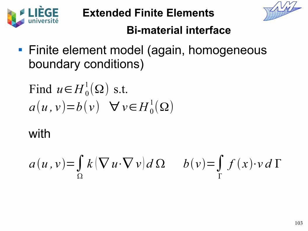
Find u∈H 01(Ω) s.t.
a(u , v)=b(v) ∀ v∈H 01(Ω)
a u , v =∫
k ∇ u⋅∇ v d bv =∫
f x ⋅v d
Finite element model (again, homogeneous boundary conditions)
with

104
Extended Finite Elements
Bi-material interface
A AInterface
T
We want to be able to represent the right temperature profile along the interface
A-A cut : Theoretical temperature profile

105
Extended Finite Elements
Bi-material interface
InterfaceT
Finite elements
The discontinuity is on the derivative of T If the interface is exactly on element
boundaries, then the discontinuity is naturally belonging to the function space

106
Extended Finite Elements
Bi-material interface
InterfaceT
The discontinuity is on the derivative of T If the interface is not exactly on element
boundaries, then ...

107
Extended Finite Elements
Bi-material interface
Exact solution Standard F.E. solution
This explains the very approximate solution...

108
Extended Finite Elements
Bi-material interface
u x =∑i∈
i N i x ∑j∈C
j* N j x ⋅F x
F 1x =∣ls x ∣
x
F
The idea here is to enrich the function space so that the discontinuity (in the gradient) belong to it.
There exists many possibilities. One very simple is using directly the absolute value of the level-set.

109
Extended Finite Elements
Bi-material interface
Definition of the set C of the enriched nodes This time, the nodes where at least one element of
the support are cutmust be enriched
In particular, if theinterface is alongedges, there is noenrichment

110
Extended Finite Elements
Bi-material interface
x
F
F 2(x)={|ls( x)|in cut elements1else
F 3 x =∑i
∣lsi∣⋅N i x −∣∑i
lsi⋅N i x ∣
F 1 x
F 2 x
F 3 x
Here are some other enrichment functions

111
Extended Finite Elements
Bi-material interface
F 3 x
F 2 xF 3 x
1 2
QT
F 1 x
Practically speaking, gives the best results
On a simple model problem, the functions and are unable to give back the exact solution (which is linear by parts) when the interface does not belong to the mesh, but does.

112
Extended Finite Elements
Bi-material interface
Solution without enrichment Solution with enrichment
Comparison of the solution with the right enrichment function

113
Extended Finite Elements
Bi-material interface
Exact solution Solution with enrichment
Comparison of the solution with the right enrichment function

114
Extended Finite Elements
Bi-material interface
Solution without enrichment Solution with enrichment
Comparison of the gradient

115
Extended Finite Elements
Bi-material interface
Exact solution Solution with enrichment
Comparaison du gradient

116
Extended Finite Elements
Bi-material interface
Convergence

117
Extended Finite Elements
More applications
Discontinuities in the primal variable Cracks
non linearities, plasticity Dynamic effects (fast propagation)
Solidification front propagation hydrogels
Discontinuities in the derivatives Homogeneization

118
Extended Finite Elements
More applications
Applications to other materials Confined plasticity Composites materials Piezoelectric materials Etc...

119
Extended Finite Elements
More applications
Direct interfaces with CAD for numerical simulations
From an explicit representation to an implicit representation
Non conforming boundaries Imposition of boundary conditions Non conforming material interfaces

120
Extended Finite Elements
More applications
Applications in explicit dynamics Non conforming geometry → issue with the critical
time step Propagation of unstable cracks (change of function
space at the crack tip → leads to problems of energy conservation)

121
Extended Finite Elements
More applications
Explicit dynamics : case without enrichment
f(t)
t

122
Extended Finite Elements
The issue of boundary conditions on implicit volumes

123
Extended Finite Elements
Goal
Free the mesh from geometrical constraints Boundaries of the problem And/or interfaces between different materials

124
Extended Finite Elements
Applications
Direct use of CAD models for the analysis Mesh generation shall be minimalistic
Use of “dirty” geometrical date not usually adapted to mesh generation
Tomography, biomedical applications Mobile interfaces
Thermoplastic mold filling Topological shape optimization
Contact problems in mechanical engineering

125
Extended Finite Elements
CAD interface
From a traditional CAD (B-rep) representation ...

126
Extended Finite Elements
CAD interface
… To an implicit representation with level-sets

127
Extended Finite Elements
Boundary conditions
How to apply boundary conditions Neumann/natural boundary conditions (e.g.
pressure, forces, gradients) Using integration (it is a
linear form)
Beware ! The integration is made on a domain ΓN
(or Ω) that cut elements in the mesh
a u ,v=∫
∇su : D : ∇
sv d
b v=∫
f⋅v d ∫N
f⋅v d N
Find u s.t.a(u , v)=b( v) ∀ v

128
Extended Finite Elements
Boundary conditions
How to apply boundary conditions Dirichlet/essential boundary conditions (e.g. :
displacements, temperature) “standard” FEM
elimination of DoFs andadding a contribution inthe right hand side
Here, the domain ΓD on
which to apply this methodis non conforming thereforeone cannot simply eliminate DoFs- one needs to compute the values to impose at each concerned DoF; so that the “right” Dirichlet BC is obtained on the boundary

129
Extended Finite Elements
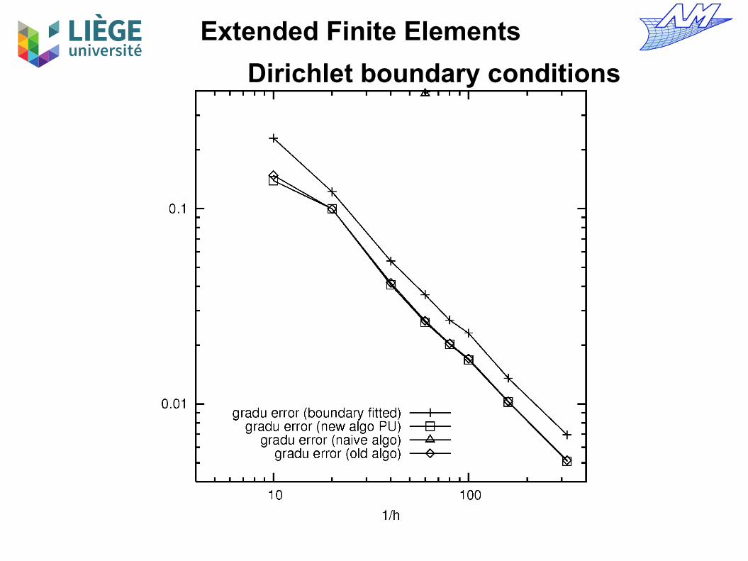
Dirichlet boundary conditions
Example 1: a simple Laplacian
Find u∈V 1={v∈H 1(Ω) , v|ΓD
=uD }s.t.
a(u , v)=b(v) ∀ v∈V 0={v∈H 1(Ω) , v|ΓD
=0 }a u , v =∫
∇ u⋅∇ v d
bv =∫N
f⋅v d

130
Extended Finite Elements
Dirichlet boundary conditions
Example 1 Dofs which are concerned : those where the
support cuts the boundary...
Matter
Void

131
Extended Finite Elements
Dirichlet boundary conditions
With only two linear elements ? Without Dirichlet B.S. : 4 DoFs , u has some
freedom in the red part If one imposes exactly u=0 on the boundary …
How many DoFs left for the red part of the domain ?
u=0
u1
a1
a2
b2
b3 c
3
c4
u3
u2 u
4
u1
a1
=u2
a2
;u2
b2
=u3
b3
;u3
c3
=u4
c4

132
Extended Finite Elements
Dirichlet boundary conditions
Concrete example Number of available DoFs after imposing exactly
the Dirichlet B.C. :
3 ! The function space is very poor in the elements crossed
by the interface, therefore the F.E. solution will be far from accurate.
Matter
Voidu=0
1 11 !

133
Extended Finite Elements
Dirichlet boundary conditions
One cannot impose exactly a Dirichlet B.C. by elimination as long as it is crossing through finite elements !
For this, an interpolation is preferred and the B.C. must be along element edges.
This is the reason why Lagrange F.E. are so widely used.
(One) solution : the use of lagrange multipliers, see an article of Babuska (1973) - in the bibliography)

134
Extended Finite Elements
Lagrange multipliers
π(u , v)=u2+v2On wants to minimize
If one sets an additional condition :
Method 1 : elimination of v :
This is the method used just before ...
δ π(u , v)=2uδ u+2v δ v=0 ∀δu ,δvu=v=0 π(0,0)=0
g (u , v)=u−v+2=0
π ' (u)=2u2+4 u+4≡π(u , v)
δ π ' (u)=4(u+1)δ u=0 ∀δ uu=−1 π ' (−1)=2→v=1

135
Extended Finite Elements
Lagrange multipliers
δ~π(u , v ,λ)=0=(2 u+λ)δu+(2 v−λ)δ v+(u−v+2)δ λ ∀δu ,δv ,δλ
Method 2 : Introduction of an additional variable
~π(u , v ,λ)=π(u , v)+λ g (u , v)=u2+v2
+λ(u−v+2)
{2 u+λ=02 v−λ=0u−v+2=0
⇔{u=−1v=1λ=2

136
Extended Finite Elements
Lagrange multipliers
In finite elements, this gives us :
−Δ u= f in Ωu=uD on ΓD
F (u)=12∫Ω
∇ u⋅∇ u d Ω−∫Ω
fu d ΩEquivalen to minimizeif the conditions of Lax-Milgram’s theorem are satisfied.
, for all u satisfying the B.C. on . By using Lagrange multipliers for the BC’s, one gets a new functionnal to minimize:
D
~F (u ,λ)=12∫Ω
∇ u⋅∇ u d Ω−∫ΓD
λ(u−uD)d ΓD−∫Ω
fu d Ω
∫Ω
∇ u⋅∇δ u d Ω=∫Ω
f δ u d Ω ∀δ uof weak form: find u s.t.
a(u ,δ u)=l (δu)
=12
a(u , u)−l (u)

137
Extended Finite Elements
Lagrange multipliers
Associated weak form : ~F (u , λ)=
12∫Ω
∇ u⋅∇ u d Ω−∫ΓD
λ(u−uD)d ΓD−∫Ω
fu d Ω
=12
A(U , U )−L(U ) U=(uλ )
A(U ,U )=(u ,λ)⋅(a bb 0)⋅(u
λ)=a(u ,u)+b(u ,λ)+b(λ , u)
L(U )=l (u)+c (λ)a(u , v)=∫
Ω
∇ u⋅∇ v d Ω
b(u ,λ)=b(λ , u)=−∫ΓD
u⋅λΓD
l u =∫
fu d
c(λ)=−∫ΓD
uD d ΓD
A(U ,δU )=L(δU )
a(u ,δ u)+b(λ ,δ u)=l (δu)
b(δ λ , u)=c(δλ)

138
Extended Finite Elements
Dirichlet boundary conditions
Find u∈V ={v∈H 1(Ω)}
λ∈L={μ∈H 1/2(ΓD)
' }s. t.
∫Ω
∇ u⋅∇ v d Ω−∫ΓD
λ⋅v d Γ=∫ΓN
f⋅v d Γ ∀ v∈V
−∫ΓD
μ⋅u d Γ=−∫ΓD
μ⋅uD d Γ ∀μ∈L
The Dirichlet B.C. has been "dualized".This is now a Neumann B.C. on the lagrange multipliers
To simplify notations, lets assign v=δu ,μ=δλ

139
Extended Finite Elements
Dirichlet boundary conditions
The Lagrange multipliers have a physical meaning In mechanics, it is the force to impose so that the
condition on the primal variable is ensured (here, displacements).
In our case, it is the gradient of the solution (flux) to impose so that u=u
D on Γ
D.
We have now a saddle point problem (min-max) – the matrix of the linear system is not definite positive anymore (but still has an inverse and is symmetric)
Not all solvers are able to handle that – mostly direct solvers and very few iterative solvers.

140
Extended Finite Elements
Dirichlet boundary conditions
How to build adequate discrete function spaces
One do not change the primal functional space (for u). It is the usual finite element space using nodal hat functions
One need to build a function space for λ. Lets try to use an identical function space L
h for λ (or the
restriction to the boundary of tsuch a space… (the trace)
Find uh∈V h⊂V ={v∈H 1(Ω)}
λh∈Lh⊂L={μ∈H 1 /2(ΓD)
' }s. t. ...

141
Extended Finite Elements
Dirichlet boundary conditions
Matter
Void
Lets try to use an identical function space Lh for λ (or the
restriction to the boundary of tsuch a space… (the trace)
Lets perform a computation. The linear system hasthe following shape :
(Ah BhT
Bh 0 )(uh
λh)=(
F h
Dh)
∫Ω
∇ u⋅∇ v d Ω−∫ΓD
λ⋅v d Γ=∫ΓN
f⋅v d Γ ∀ v∈V h
−∫ΓD
μ⋅u d Γ=−∫ΓD
μ⋅uD d Γ ∀μ∈Lh

142
Extended Finite Elements
Dirichlet boundary conditions
The we solve it … Lagrange multipliers
are oscillating. The more h (element
size) shrinks, the more it oscillates...

143
Extended Finite Elements
Dirichlet boundary conditions
What happens ? The discrete spaces for u et λ are incompatible. Those do not satisfy the Ladyzhenskaya-Babuška-
Brezzi (LBB) condition, or inf-sup condition :
This condition is difficult to check analytically.
O. Ladyzhensakya, Global solvability of a boundary value problem for the Navier–Stokes equations in the case of two spatial variables. Proc. Ac. Sc. USSR 123 (3) (1958) 427–429.I. Babuska, Error bounds in the finite element method, Numer. Math., 16 (1971), pp. 322-33.F. Brezzi, On the existence, uniqueness and approximation of saddle-point problems arisingfrom Lagrangian multipliers, RAIRO, Anal. Num., 8, R2 (1974), pp. 129-151
infμ∈Lh
supu∈V h
∫Γ
λhuhd Γ
h1/2‖λ‖0,ΓD‖u‖1,Ω
≥α>0

144
Extended Finite Elements
Dirichlet boundary conditions
Numerical validation of the LBB condition. There exists a “simple” numerical test; see
Chapelle, Bathe, 1993 and KJ Bathe 2001 (in the bibliography)
One considers a mor general problem with an added “stiffness” on the dirichlet boundary condition (becomes a Robin B.C.) – if k → , back to a “hard” Dirichlet B.C.
(Ah Bh
T
Bh −1k
M h)(uh
λh)=(F h
Dh)
∫Ω
∇ u⋅∇ v d Ω−∫ΓD
λ⋅v d Γ=∫ΓN
f⋅v d Γ ∀ v∈V h
−∫ΓD
μ⋅u d Γ−∫ΓD
1kλμ d Γ=−∫
ΓD
μ⋅uD d Γ ∀μ∈Lh

145
Extended Finite Elements
Dirichlet boundary conditions
Chapelle – Bathe numerical test
It amounts to check the first non vanishing eigenvalue (b
0) of the following eigenproblem :
ou A
h must have an inverse
Does not depend on k ! One checks that b
0 does not vanish for a sequence of
meshes with an increasing density Here, (and for : see slides before)
(Ah Bh
T
Bh −1k
M h)(uh
λh)=(
F h
Dh)
=0
1h
( Bh Ah−1 Bh
T )W h=b M h W h
1h
( BhT M h
−1 Bh )W h'=b
' Ah W h'
α

146
Extended Finite Elements
Dirichlet boundary conditions
Results Two cases :
- aligned with the mesh
- non conforming The second case
does not workat all.

147
Extended Finite Elements
What we have are incompatibles functional spaces...
The space for the Lagrange multipliers is way too “rich” with respect to the one for the primal variable.
It amounts to impose exactly the Dirichlet B.C., which has beed already shown to be a bad idea.
→ We have to “decimate” Lh
Dirichlet boundary conditions

Extended Finite Elements
Dirichlet boundary conditions
●From the mesh of the interface, take each node and put it in a set N●If a node of N is also part of the mesh, mark it as Vital (set V) , and delete it from N●Take each edge incident to N and count each intersecting edge going from end nodes with the interface●Sort N. The sorting key is the number defined above (smallest first)
●Loop over the sorted set N, take ni● Take the end nodes of ni, and from those, the connected nodes in N (may be many)● If ni is not yet NV (non vital), mark it as Vital (V) and all the other connected nodes as (NV)
●EndLoop
2
2
3 4 4 5
4
6 46
4 5 4 4 4
5 4 6
4
5 4 4 4 4 4 4 4 4 3

Extended Finite Elements
Dirichlet boundary conditions
What remains, An approximately uniform distribution of nodes
The density is same as the initial mesh (2D here, 3D in general
Works in 3D !

Extended Finite Elements
Dirichlet boundary conditions
Result of the decimation Projection of 3D nodes

Extended Finite Elements
Dirichlet boundary conditions
Projection of 3D nodesResult of the decimation

Extended Finite Elements
Dirichlet boundary conditions
How to build shape functions from this ? Directly on the interface ?
Works...
… only in 2D !!!

Extended Finite Elements
Dirichlet boundary conditions In 3D : one would have to build a triangulation
of the set of nodes VWhat about :
Curvy interfaces Discrepancy (non
conformity) btw. triangulations
Integration problems
So we must find a better way in 3D...

Extended Finite Elements
Dirichlet boundary conditions Another solution
Lets take the trace of volume shape functions – but there are too many !
One will combine SFs. (linear combinations) for each V-node
At some places, a volume SF may be linked to more than one V-node.
There is room for freedom : 100% with the green, or 100% with the red or whatever combination such that the sum is 100% (to keep “partition of unity”)

Extended Finite Elements
Dirichlet boundary conditions
Advantages of using trace shape function for Lagrange multipliers
Easy integration Compact shape functions Partition of unity on the interface Same algorithm in 3D and 2D Good numerical results ? See what’s follow !

Extended Finite Elements
Dirichlet boundary conditions
2D
3D

Extended Finite Elements
Dirichlet boundary conditions

Extended Finite Elements
Dirichlet boundary conditions

Extended Finite Elements
Dirichlet boundary conditions
Extended Finite Elements
Dirichlet boundary conditions

Extended Finite Elements
Dirichlet boundary conditions
Composites : perfect glueing Imperfect glueing

Extended Finite Elements
Dirichlet boundary conditions

Extended Finite Elements
Dirichlet boundary conditions

Extended Finite Elements
Dirichlet boundary conditions

165
Extended Finite Elements
Cad Interface
From a traditional CAD (B-rep) representation ...
166
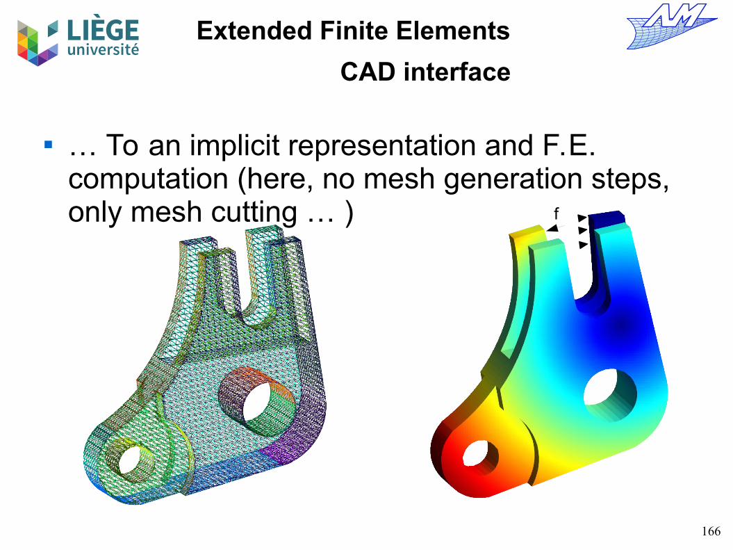
Extended Finite Elements
CAD interface
… To an implicit representation and F.E. computation (here, no mesh generation steps, only mesh cutting … ) f

167
Extended Finite Elements
Bibliography (to be completed!)
Babuska I. « The finite element method with Lagrange multipliers » Numerische Mathematik,20:179-192,1973Babuska I. Melenk J.M. « The partition of unity method » IJNME, 40:727-758,1997Barth T.J. Sethian J.A. « Numerical schemes for the hamilton-jacobi and level-set equations on triangulated domains » JCP 145:1-40,1998Bathe K.J « The inf-sup condition and its evaluation for mixed finite element methods, Computer and Structures 79:243-252, 2001Béchet E. Minnebo H. Moës N. Burgardt B. « improved implementation and robusness study of the X-FEM for stress analysis around cracks » IJNME 64:1033:1056,2005Béchet E. Scherzer M, Kuna M, « Applications of the X-FEM to the fracture of piezoelectric materials, IJNME 77:1535:1565,2009Béchet E. Moës N. Wohlmuth B. « A stable lagrange multiplier space for stiff interface conditions within the extended finite element method » , IJNME 78(8):931-954,2009.Belytschko T. Moës N, Usui S, Parimi C, « arbitrary discontinuities in finite elements » IJNME 50:993-1013,2001Belytschko T. Chessa J. Zi G. Xu J. Th extended finite element method for arbitrary discontinuities, Computational mechanics – Theory and practice » K.M. Mathisen, T. Kvamsdal et K.M. Okstad (dir), CIMNE Barcelona, Spain 2003Breitkopf P (dir) « La méthode des éléments finis – extensions et alternatives » Hermes-Lavoisier, France, 2006Chapelle D. Bathe KJ. « The inf-sup test » Computer and Structures 47:537-545, 1993Daux C Moës N. Dolbow J Sukumar N Belytschko T. « Arbitrary branched and intersecting cracks with the extended finite element method » IJNME 48:1741-1760,2000Dolbow J. Moës N. Belytschko T. « Discontinuous enrichment in finite elements with a partition of unity method » FEAD 36:235-260,2000Gravouil A. Moës N. Belytschko T. « Non planar 3D crack propagation by the extended finite element method and level-sets part II: level-set update » IJNME 53:2569-2586,2002Legrain G. Moës N. Verron E « stress analysis around crack tips in finite strain problems using the X-FEM » IJNME 63:290-314,2005Moës N. Béchet E. Toubier M. « Imposing essential boundary conditions in the extended finite element method »IJNME 67:1641-1669,2006

168
Extended Finite Elements
Bibliography (to be completed!)
Moës N. Cloirec M. Cartraud P. Remacle J.F. « a computational approach to handle complex microstructure geometries » CMAME 53:3163-3177,2003Moës N. Dolbow J. Belytschko T. « A finite element method for crack growth without remeshing », IJNME 46:133-150,1999Moës N. Gravouil A. Belytschko T. « Non planar 3D crack propagation by the extended finite element method and level-sets part I : Mechanical model IJNME 53:2549-2568,2002Osher S, Fedkiw R. « level-set methods and dynamic implicit surfaces » Springer-verlag 2002Moës, N. Stolz C. ,Bernard P.-E. , and Chevaugeon N. A level set based model for damage growth: The thick level setApproach IJNME 86:358–380 2011Mohammadi, S « Extended Finite Element Method for fracture analysis of structures» , Blackwell publishing, ISBN 978-1-4051-7060-4, 2008.Rhetore J. Gravouil A. Combescure A. « an energy conserving scheme for dynamic crack growth with the X-FEM » IJNME 63:631-659,2005Sethian J.A. « level set methods and fast marching methods : evolving interfaces in computational geometry, fluid mechanics, computer vision and material sciences »Cambridge university press, UK, 1999Sukumar N.Chopp D.L. Moës N Belytschko T. « modeling holes and inclusions by level-sets in the extended finite element method » CMAME 190:6183-6200,2001Sukumar N. Moës N. Moran B. Belytschko T. « Extended finite element method for three dimensional crack modelling » IJNME 48:1549-1570,1999Strouboulis T. Babuska I. Copps K. « The design and analysis of the generalized finite element method » CMAME 181:43-71,2000
Nota :
IJNME = International journal for numerical methods in engineering (Wiley)CMAME = Computer methods in applied mechanics and engineering (Elsevier)FEAD = Finite element in analysis and design (Elsevier)JCP = Journal of computational physics (Elsevier)