UNIVERSITY OF WARWICK

Second Year Essay

An Introduction to the Gamma Function

Tutor:Dr. Stefan Adams

April 4, 2009

Contents

1 Introduction 2

2 Convex Functions 3

3 The Gamma Function 7

4 The Bohr-Mollerup Theorem 11

5 Relation to the Beta Function 15

6 Applications and Summary 18

7 Bibliography 20

1

1 Introduction

The introduction to this essay is largely drawn from sources [1] and [2].

Traditionally, we define the factorial function to be

n! = n(n− 1)(n− 2)...(2)(1)

for all positive integers. But how can we extend this factorial function so that it includes non-integervalues? This is the simple problem posed originally by Daniel Bernoulli and Christian Goldbachin the 1720s and one which was eventually solved by Leonhard Euler in 1729. Euler expressedn! as both an infinite sum and an integral, both of which were outlined in his famous paper ”Deprogressionibus transcendentibus seu quarum termini generales algebraice dari nequeunt”.

A year later, in 1730, James Stirling found a formula to approximate n! as n gets very large.This became known as Stirling’s Formula and was refined throughout the years, however it wasnot until 1900 that Charles Hermite actually proved that Stirling’s Formula corresponds exactly toEuler’s integral.

Between 1730 and the present day, there have been many significant leaps forward in this area.Around 1812, Carl Friedrich Gauss rewrote Euler’s product as a limit of a function, as well asconsidering the factorial of a complex number. A few years later, Karl Weierstraß came up withyet another representation of what now is known as the gamma function (a suggestion put forwardby Legendre around 1811). During the late 19th century and early 20th century, both Holder’sTheorem and the Bohr-Mollerup Theorem were proved.

In this essay, we will start by introducing the concept of convex functions, which play an im-portant role in the Bohr-Mollerup Theorem, the proof of which we will also work through. We willshow that the gamma function is equivalent to the factorial function for positive integers, and wealso investigate where the function is defined and where it is not.

We will also see both Weierstraß and Gauss’ expressions for the gamma function, as well asexploring the relationship that they have with the equally famous beta function. Finally we willconclude by looking at Stirling’s Formula and seeing the many practical applications of the gammafunction.

This essay will consider real functions of one variable, but the same ideas can be applied tofunctions of multiple variables, as well as those with complex arguments.

2

2 Convex Functions

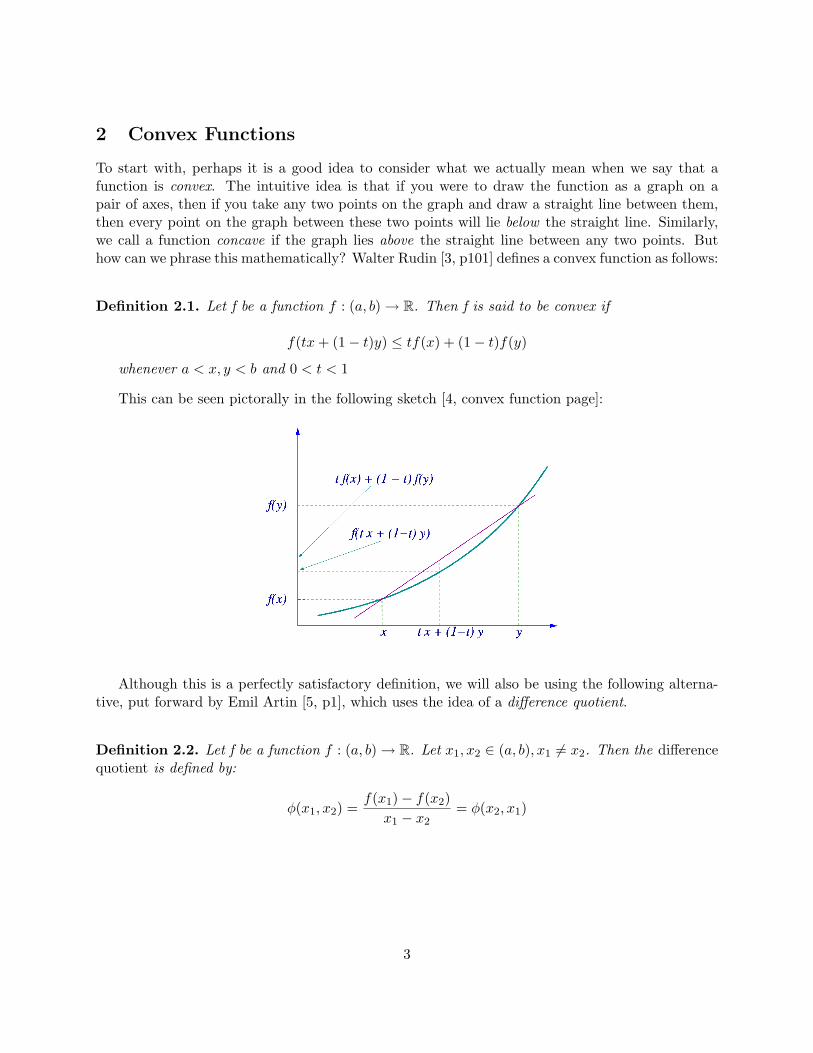
To start with, perhaps it is a good idea to consider what we actually mean when we say that afunction is convex. The intuitive idea is that if you were to draw the function as a graph on apair of axes, then if you take any two points on the graph and draw a straight line between them,then every point on the graph between these two points will lie below the straight line. Similarly,we call a function concave if the graph lies above the straight line between any two points. Buthow can we phrase this mathematically? Walter Rudin [3, p101] defines a convex function as follows:

Definition 2.1. Let f be a function f : (a, b)→ R. Then f is said to be convex if

f(tx+ (1− t)y) ≤ tf(x) + (1− t)f(y)

whenever a < x, y < b and 0 < t < 1

This can be seen pictorally in the following sketch [4, convex function page]:

Although this is a perfectly satisfactory definition, we will also be using the following alterna-tive, put forward by Emil Artin [5, p1], which uses the idea of a difference quotient.

Definition 2.2. Let f be a function f : (a, b)→ R. Let x1, x2 ∈ (a, b), x1 6= x2. Then the differencequotient is defined by:

φ(x1, x2) =f(x1)− f(x2)

x1 − x2= φ(x2, x1)

3

Also, for x1, x2, x3 ∈ (a, b), x1 6= x2 6= x3

Ψ(x1, x2, x3) =φ(x1, x3)− φ(x3, x2)

x1 − x2

The value of Ψ(x1, x2, x3) does not change when x1, x2, x3 are permuted [5, p1].

We are now in a position to define a convex function in the same way as Artin did [5, p1].

Definition 2.3. Let f be a function with f : (a, b)→ R. Then f is convex on (a, b) if∀x3 ∈ (a, b), φ(x1, x3) is a monotonically increasing function of x1.

In other words, take x1 > x2, x2 6= x3. Then

φ(x1, x3) ≥ φ(x2, x3)

=⇒ φ(x1, x3)− φ(x2, x3) ≥ 0

Now notice the left hand side of the above equation is the numerator of the three-variabledifference quotient defined above. Also recall that x1 > x2. So we can say that a function is convexif and only if for all distinct x1, x2, x3 ∈ (a, b),

Ψ(x1, x2, x3) ≥ 0.

We can now prove a few simple theorems involving convex functions, all of which will play animportant role later on when we finally meet the gamma function.

Theorem 2.1. Suppose f, g : (a, b) → R are convex functions. Then f(x) + g(x) is a convexfunction. [5, p2]

Proof. The proof is trivial and follows directly from the definition:

Suppose x1 < x2 < x3.

Then let Ψ1(x1, x2, x3) be the difference quotient of f(x) and let Ψ2(x1, x2, x3) be the differencequotient of g(x).

Then if Ψ1(x1, x2, x3) > 0 and Ψ2(x1, x2, x3) > 0 then Ψ1(x1, x2, x3) + Ψ2(x1, x2, x3) > 0 whichis precisely the difference quotient of f(x) + g(x).

Hence f(x) + g(x) is convex, as required.

4

The next theorem is a very interesting one, and one which Rudin leaves as an exercise to thereader [3, p101]. I have provided the following proof:

Theorem 2.2. Let f : (a, b)→ R be a convex function. Then f is continuous.

Proof. Let c be a point such that a < c < b

Now construct two straight lines, one from (a, f(a)) to (c, f(c)) and the other from (c, f(c)) to(b, f(b)). Note that these two lines intersect at (c, f(c)).

Consider the equations of these two lines. They can simply be written as:

L1 =f(c)− f(a)

c− a(x− c) + f(c),

and

L2 =f(b)− f(c)

b− c(x− c) + f(c).

Now suppose x < c.Since f is convex, f(x) is sandwiched between these two lines. So we can say:

f(c)− f(a)c− a

(x− c) + f(c) < f(x) <f(b)− f(c)

b− c(x− c) + f(c)

Now let x→ c. So we have:

f(c) < limx→c

f(x) < f(c).

Hence by the Sandwich Lemma,limx→c

f(x) = f(c).

A similar arguement can be used if x > c as we simply swap the inequality signs around in theabove expression. So we know that ∀x ∈ (a, b), if x→ c then f(x)→ f(c).

So we can say f is continuous, as required.

Note that the converse to the above theorem is not true. Clearly not all continuous functionsare convex! (Just take f(x) = x3). Also note that the theorem does not hold if f is defined on theclosed interval. Let f : [0, 1] → R with f(x) = 0 if x < 1 and f(1) = 1. Clearly this function isconvex, yet it is of course not continuous.

5

Theorem 2.3. Let f be a twice differentiable function. Then f is convex if and only iff ′′(x) ≥ 0 for all x in the open interval where f(x) is defined.

Proof. The proof for this is outlined in Artin [5, p4] and the result will be very useful later on.

We are now ready to introduce the concept of log-convex functions [5, p7], which are definedexactly as you may think they would be.

Definition 2.4. Let f : (a, b)→ R be a function such that f(x) > 0 ∀x ∈ (a, b). Then f is said tobe log-convex if log(f(x)) is a convex function.

Note that f(x) > 0 ∀x ∈ (a, b) is an important condition, otherwise log(f(x)) would not be de-fined on the whole interval. The following theorem provides a test to see if a function is log-convex[5, p7].

Theorem 2.4. Suppose f : (a, b)→ R is a twice differentiable function. If ∀x ∈ (a, b),

i) f(x) > 0, andii) f(x)f ′′(x)− (f ′(x))2 ≥ 0,

then f is log-convex.

Proof. Firstly consider log(f(x)). This is differentiable as it is a composition of two differentiablefunctions. So we can use the Chain Rule:

(logf(x))′ =f ′(x)f(x)

.

Now we simply differentiate once more using the quotient rule. So

(logf(x))′′ =f(x)f ′′(x)− f ′(x)f ′(x)

f(x)f(x)=f(x)f ′′(x)− (f ′(x))2

(f(x))2.

So by Theorem 2.3, logf(x) is convex if and only if (logf(x))′′ ≥ 0 ∀x ∈ (a, b).

Since we have calculated (logf(x))′′, we can say that logf(x) is convex if and only if f(x)f ′′(x)−(f ′(x))2 ≥ 0 and f(x) > 0. Hence, we have shown that if conditions i) and ii) are satisfied, then fis log-convex.

This concludes our section on convex functions, and supplies us with the tools that we need toinvestigate the gamma function.

6

3 The Gamma Function

In this section, we will finally define the gamma function in the same way that Euler did, as wellas deriving the recurrence relation relating to the function.

Definition 3.1. Let x be a real number that isn’t zero or a negative integer. Then the gammafunction, denoted by Γ, is defined as:

Γ(x) =∫ ∞

0tx−1e−tdt

Note that the above integral is not defined for all values of x. In fact we can only say that Γ(x)is defined everywhere except at 0 and for negative integers. We will see why this is the case lateron. For now though, let us derive the famous recurrence relation by evaluating the integral. Thissection is largely based on [6, Appendix C, pp 1-3].

We use integration by parts (assuming x 6= 0) to obtain

Γ(x) =[e−t tx

x

]∞0

+∫ ∞

0

e−t tx

xdt

=[e−t tx

x

]∞0

+1x

∫ ∞0

e−t tx dt.

Now consider the first term of the RHS of the above equation.

[e−t tx

x

]∞0

=[e−t tx

x

]t=∞−[e−t tx

x

]t=0

=[e−t tx

x

]t=∞

= limt→∞

(tx

x et

)

7

Since this term is continuous and differentiable and (x et)′ 6= 0 ∀t ∈ R, we can use L’Hopital’sRule to evaluate it. Assume x > 0 and take m ≥ x. Also note these conditions hold for subsequentiterations of L’Hopital’s Rule so we have,

limt→∞

(tx

x et

)= lim

t→∞

d

dt(tx)

d

dt(x et)

= ... = limt→∞

dm

dtm(tx)

dm

dtm(x et)

= limt→∞

x(x− 1)(x− 2)...(x−m+ 1) tx−m

x et

= limt→∞

(x− 1)(x− 2)...(x−m+ 1)tm−x et

= 0.

So it has become clear that we now have

Γ(x) =1x

∫ ∞0

e−t tx dt.

But now we can compare this to the original definiton that we have of the gamma function,

Γ(x) =∫ ∞

0tx−1e−tdt =

1x

∫ ∞0

e−t tx dt

So observe that Γ(x) =1x

Γ(x+ 1) or alternatively,

Γ(x+ 1) = xΓ(x).

Now consider the case when x = 1. From the definition,

Γ(1) =∫ ∞

0e−tdt =

[−e−t

]∞0

= 1.

8

So Γ(1) = 1 = 0!

Now we simply use the recurrence relation we have just derived, and induction on x as follows:

We know Γ(1) = 0!Assume Γ(x+ 1) = x!So Γ(x+ 2) = (x+ 1) Γ(x+ 1) = (x+ 1)x! = (x+ 1)!

Hence it is clear that in general, Γ(x+ 1) = x! for x = 1, 2, 3, ...

Hence we have shown that the factorial function is simply a specific case of the gamma function.

Now you may think that the above defines the gamma function for all real numbers with theexception of 0, since clearly the above working becomes meaningless if x = 0 (due to the x in thedenominator). However this is not the whole story. Let us assume that we know the value of thegamma function in the interval 0 < x ≤ 1. Then using the recurrence relation that we have justderived, it becomes clear that we can calculate the value of the gamma function for all positive realvalues of x.

Now consider the case when x < 0. Again, we can use the recurrence relation to calculate thevalue of Γ(x) if x is a non-integer. However, if x is a negative integer, the recurrence relation willrequire us to know the value of Γ(0), which is, as we know, undefined. Hence the gamma functionis also undefined if x is a negative integer. To verify this reasoning, observe the following examples(Note: the values of Γ(x) for x ∈ (0, 1) were simply obtained using Matlab, however there are manytables that have been published with these values in them).

Example 3.1. Γ(1.7) = 0.7 Γ(0.7) = (0.7)(1.298) = 0.9086

Example 3.2. Γ(−0.4) =Γ(0.6)−0.4

=1.4892−0.4

= −3.723

Example 3.3. Γ(−2) =Γ(−1)−2

=Γ(0)

2

But we know that Γ(0) is undefined and hence so is Γ(−2).

9

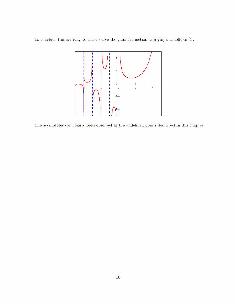
To conclude this section, we can observe the gamma function as a graph as follows [4].

The asymptotes can clearly been observed at the undefined points described in this chapter.

10

4 The Bohr-Mollerup Theorem

So far we have considered the concept of convex functions, as well as defining and investigatingthe properties of the gamma function. Now we can combine what we have seen in the previoustwo chapters to help us state and prove possibly the most famous theorem relating to the gammafunction: The Bohr-Mollerup Theorem. The proof is very elegant and is one of my favourites thatI have come across so far in analysis. The following draws heavily on [5, pp14-15].

Theorem 4.1. If a function f satisfies the following three conditions, then it is identical in itsdomain of definition with the gamma function.

i) f(x+ 1) = x f(x).ii) The domain of definition of f contains all x > 0 and is log-convex for these values of x.iii) f(1) = 1.

Proof. Suppose f(x) satisfies the above three conditions. We know that there exists such a func-tion, since the gamma function does indeed satisfy all three conditions. So we must show that thissolution is unique.

Observe that f(x+ 1) = x f(x) and f(x+ 2) = (x+ 1) f(x+ 1) = (x+ 1)x f(x)

So in general, f(x+ n) = (x+ n− 1) (x+ n− 2)...(x+ 1)x f(x) holds.Let us call this equation † .

Since f(1) = 1 by iii), then f(n) = (n− 1)! ∀n ∈ N, n > 0

So it suffices to show that f(x) agrees with Γ(x) on the interval 0 < x ≤ 1 as if this holds thenby condition i), it will agree with Γ(x) everywhere.

Let x ∈ R, x ∈ (0, 1] and n ∈ N s.t. n ≥ 2.

Now let us consider the difference quotients, φ(x1, n), for different values of x1. By conditionii), f is log-convex and so φ(x1, n) is a monotonically increasing function of x1. So we obtain theinequality,

logf(−1 + n)− logf(n)(−1 + n)− n

≤ logf(x+ n)− logf(n)(x+ n)− n

≤ logf(1 + n)− logf(n)(1 + n)− n

Now since f(n) = (n− 1)!, we have,

11

(−1)log(n− 2)!− log(n− 1)! ≤ logf(x+ n)− log(n− 1)!x

≤ logn!− log(n− 1)!

(−1)(log

(n− 2)!(n− 1)!

)≤ logf(x+ n)− log(n− 1)!

x≤ log

(n!

(n− 1)!

)

log(n− 1) ≤ logf(x+ n)− log(n− 1)!x

≤ log(n).

We can continue to rearrange the inequalities so that

xlog(n− 1) + log(n− 1)! ≤ logf(x+ n) ≤ xlog(n) + log(n− 1)!

log[(n− 1)x(n− 1)!] ≤ logf(x+ n) ≤ log[nx(n− 1)!].

Now since log is monotonic also, we can say,

(n− 1)x(n− 1)! ≤ f(x+ n) ≤ nx(n− 1)!

Now we substitute † into the above equation so

(n− 1)x(n− 1)! ≤ f(x)x(x+ 1)...(x+ n− 1) ≤ nx(n− 1)!

We now rearrange this inequality to leave f(x) sanwiched between two other functions:

(n− 1)x(n− 1)!x(x+ 1)...(x+ n− 1)

≤ f(x) ≤ nx(n− 1)!x(x+ 1)...(x+ n− 1)

=(

nxn!x(x+ 1)...(x+ n)

)(x+ n

n

).

12

Since this holds ∀n ≥ 2, we can replace n by n+ 1 on the LHS of the equation. So,

nxn!z(x+ 1)...(x+ n)

≤ f(x) ≤(

nxn!x(x+ 1)...(x+ n)

)(x+ n

n

).

Now from above it is is quite clear that

a)nf(x)x+ n

≤(

nxn!x (x+ 1)...(x+ n)

), and

b)(

nxn!x (x+ 1)...(x+ n)

)≤ f(x), so we can say

f(x)n

x+ n≤(

nxn!x (x+ 1)...(x+ n)

)≤ f(x).

Now let n→∞. Since limn→∞

(n

x+ n

)= 1, by the Sandwich rule,

limn→∞

(nxn!

x (x+ 1)...(x+ n)

)= f(x).

But we know that Γ(x) satisfies our three conditions, so we can replace f(x) with Γ(x) on theRHS of the above equation. From Analysis I, we know that limits are unique, and hence Γ(x) isthe only function that satisifes the three criteria. Hence we have completed the proof.

Note that the above proof only considered x ∈ (0, 1]. The gamma function is not just definedon this interval, so we must show that proving the theorem on this interval actually proves it forall x where Γ(x) is defined. The following corollary helps us to see this.

Corollary 4.1.

Γ(x) = limn→∞

(nxn!

x (x+ 1)...(x+ n)

)∀x where Γ(x) is defined.

13

Proof. Firstly, let us denote the fraction inside the limit by Γn(x)

Now Γn(x+ 1) =(

nx+1n!(x+ 1) (x+ 2)...(x+ n+ 1)

)= xΓn(x)

(n

x+ n+ 1

).

So now can rearrange the above to give

Γn(x) =(

1x

) (x+ n+ 1

n

)Γn(x+ 1).

This shows that if limn→∞ Γn(x) exists, then it also exists for Γn(x+ 1). Conversely, if it existsfor Γn(x+ 1), x 6= 0, then it also exists for Γn(x).

So the limit exists exactly for all values where Γ(x) is defined.

The above representation of the gamma function was first derived by Gauss [1], however thereare still further ways in which the gamma function can be expressed. I shall just touch upon theform derived by Weierstraß here. Observe the following

Γn(x) =(

nxn!x (x+ 1)...(x+ n)

)

=(

nxn!x (1 + x) (1 + x/2)...(1 + x/n)

)

With some further manipulation, we can express Γ(x) as such [7, p180]:

1Γ(x)

= x eγ x∞∏n=1

[(1 +

x

n

)e−x/n

].

whereγ = lim

n→∞(1 + 1/2 + ... + 1/n− logn)

is Euler’s constant [7, p150]. This simply illustrates the fact that Γ(x) can be written in morethan one way.

14

5 Relation to the Beta Function

So now that we have seen the gamma function and its various representations, we can move on toanother important function in analysis, the beta function, which we will see is very closely linkedto the gamma function. Firstly though, let us define it [3, p193].

Definition 5.1. Let x, y ∈ R be non-negative. Then the beta function is defined as

B(x, y) =∫ 1

0tx−1(1− t)y−1dt.

The following theorem shows the relationship between the gamma and beta functions very well,and the proof shall be worked through using [3, pp193 - 194] and [5, pp18 - 19] as a guide.

Theorem 5.1. Suppose x, y are real numbers that aren’t zero or negative integers. Then,

B(x, y) =Γ(x) Γ(y)Γ(x+ y)

.

Proof. Consider

B(x+ 1, y) =∫ 1

0tx(1− t)y−1dt

=∫ 1

0

(t

1− t

)x(1− t)x(1− t)y−1 dt

=∫ 1

0

(t

1− t

)x(1− t)x+y−1 dt.

Now let us use integration by parts to get

15

B(x+ 1, y) =[(−(1− t)x+y

x+ y

)(t

1− t

)x ]1

0

+∫ 1

0

x

x+ y(1− t)x+y

(t

1− t

)x−1 1(1− t)2

dt

=x

x+ y

∫ 1

0tx−1[(1− t)x+y (1− t)1−x (1− t)−2 ] dt

=x

x+ y

∫ 1

0tx−1(1− t)y−1 dt

=x

x+ yB(x, y).

Now let us take y to be fixed. To satisfy Γ(x+ 1) = xΓ(x), let us set f(x) to be

f(x) = B(x, y)Γ(x+ y)

We will call this equation ?.Now consider the three conditions in the Bohr-Mollerup Theorem (Thm 4.1). We see f satisfies

condition i) since we have chosen it specifically to do this.

The function f also satisfies condition ii) since it a product of two log-convex functions andhence is log-convex also [5, p18]. The proof that B(x, y) is log-convex is long and not very inter-esting and so shall not be reproduced here.

Condition iii), however, is more tricky. Note that

B(1, y) =∫ 1

0(1− t)y−1 dt =

1y.

So we have

f(1) = B(1, y) Γ(1 + y)

=1y

Γ(1 + y)

= Γ(y).

But we want f(1) = 1 for iii) to be satisfied. So instead of f(x), consider f(x)/f(1) instead.Now this satisfies all three conditions, so

16

Γ(x) = f(x)/f(1).

But f(1) = Γ(y) as we saw above. Hence we have

f(x) = Γ(x)Γ(y).

So let us substitute this back into ? and we see that

B(x, y) =Γ(x)Γ(y)Γ(x+ y)

.

This theorem can help us to see an interesting result regarding the gamma function [3, p194].Consider x = y = 1/2. So

Γ(1/2)Γ(1/2)Γ(1)

= B(1/2, 1/2) =∫ 1

0t−1/2(1− t)−1/2dt.

Now we can use a simple substitution (let t = sin2 θ) to see that

[Γ(1/2)]2 =∫ π/2

0(sin θ)−1(1− sin θ)−1/2 sin 2θ dθ

=∫ π/2

0(sin θ)−1(cos θ)−1 sin 2θ dθ

=∫ π/2

0

sin 2θsin θ cos θ

dθ

=∫ π/2

0

sin 2θ1/2 sin 2θ

dθ

= 2∫ π/2

01 dθ

= π.

Hence we have Γ(1/2) =√π. So we can see that for any real number of the format n + 1/2

(where n is an integer), Γ(x) is easy to calculate using the recurrence relation derived in §3.

17

6 Applications and Summary

There is so much more to the gamma function than the content covered in this essay; I have sim-ply chosen the most important and interesting aspects to write about. I will use this final coupleof pages to very briefly touch upon what else can be done with the gamma function, and it willhopefully inspire the reader to investigate this topic further. If the reader does indeed wish to readmore about the gamma function, then I recommend Emil Artin’s paper as a great place to start.Alternatively the reader could go straight to Euler’s paper mentioned in the introduction.

Firstly, thanks to James Stirling, we are able to approximate Γ(x) for large values of x andhence we are able to approximate n! when n gets very large. This is given by [6, §C, p9]

n! = limn→∞

√2πn

(ne

)n.

This can be extended to approximate the gamma function for large values - this is explainedwell in [5, p24].

Another interesting theorem regarding the gamma function is Holder’s Theorem, which statesthat the gamma function does not satisfy any algebraic differential equation [1]. The gamma func-tion does not appear to satisfy any simple differential equations, but this has currently not beenproven.

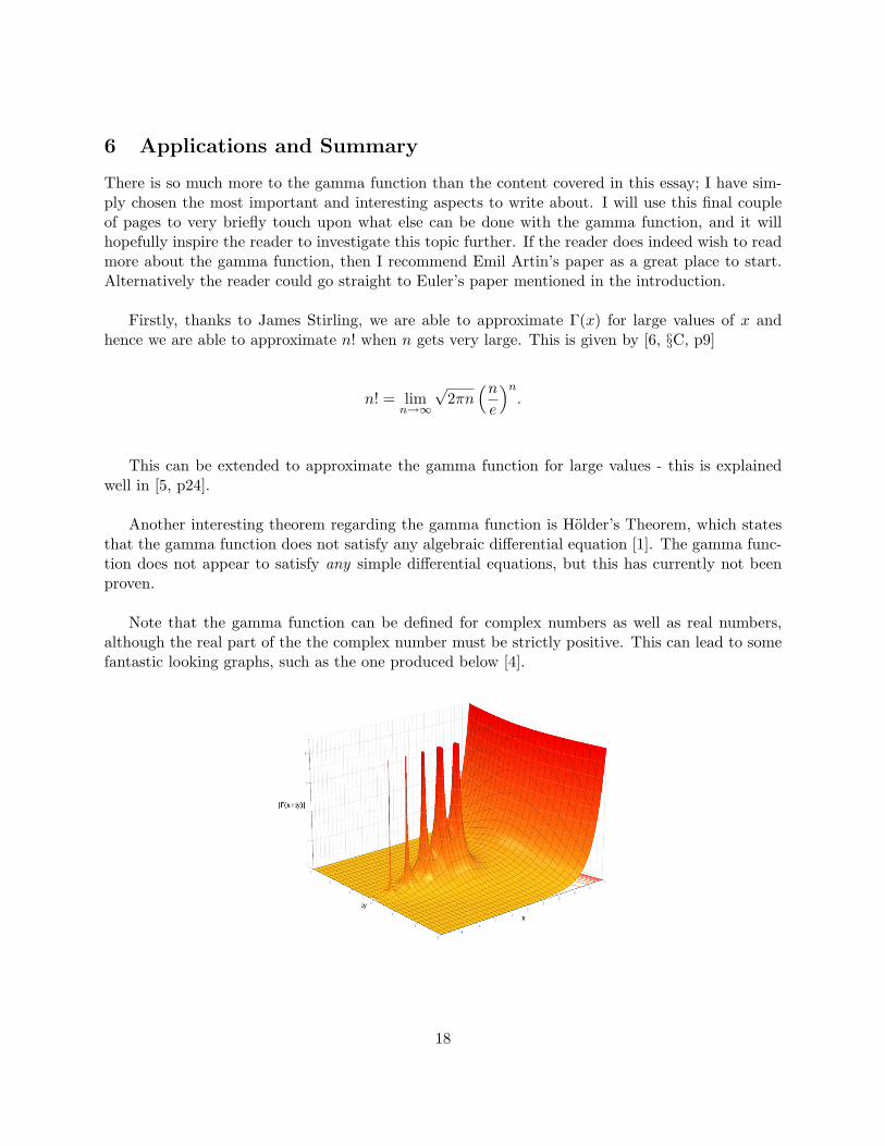
Note that the gamma function can be defined for complex numbers as well as real numbers,although the real part of the the complex number must be strictly positive. This can lead to somefantastic looking graphs, such as the one produced below [4].

18

The gamma function is also the basis for the gamma distribution, which is used frequently tomodel waiting times (such as time until death, time until the next bus comes) [8, §3.3]. There aremany more applications of the gamma function, including its use in various integration techniquesand its importance to the beta function (as we have seen). It is also used frequently in combinatoricsto calculate power series and in analytic number theory to allow further study into the famousRiemann zeta function [1]. This shows that the gamma function is not just a mathematical curiosity;it really is worth studying as it opens up so many more mathematical possiblities that simplywouldn’t be possible without it.

19

7 Bibliography

[1] Citizendium. An online encyclopedia. http://en.citizendium.org/wiki/Gamma function

[2] Wolfram. A wolfram web resource. http://functions.wolfram.com/GammaBetaErf/Gamma/35/

[3] Principles Of Mathematical Analysis. Walter Rudin. McGraw-Hill Inc. 1976

[4] Wikipedia. An online resource. http://en.wikipedia.org/wiki/Gamma function

[5] The Gamma Function. Emil Artin. Holt, Rinehart and Winston, Inc. 1964

[6] Mathematics for Business, Science and Technology. S. Karris. Orchard Publications 2007

[7] Dictionary of Mathematics. David Nelson. Penguin Group 2003

[8] Introduction To Mathematical Statistics. R.Hogg and A.Craig. New York: Macmillan 1978

20