an introduction to the mathematical theory of nonlinear ... · of nonlinear control systems ......
TRANSCRIPT

An Introduction to the Mathematical Theory
of Nonlinear Control Systems
Alberto Bressan
S.I.S.S.A., Via Beirut 4, Trieste 34014 Italyand
Department of Mathematical Sciences, NTNU, N-7491 Trondheim, Norway
1. Definitions and examples of nonlinear control systems
2. Relations with differential inclusions
3. Properties of the set of trajectories
4. Optimal control problems
5. Existence of optimal controls
6. Necessary conditions for optimality: the Pontryagin Maximum Principle
7. Viscosity solutions of Hamilton-Jacobi equations
8. Bellman’s Dyanmic Programming Principle and sufficient conditions for opti-mality
0
Control Systems
x = f(x, u) x ∈ IRn, u ∈ U ⊂ IRm (1)
x(0) = x0 (2)
A trajectory of the system is an absolutely continuousmap t 7→ x(t) such that thereexist a measurable control function t 7→ u(t) ∈ U , such that x(t) = f
(x(t), u(t)
)for
a.e. t ∈ [0, T ].
Basic assumptions
1 - Sublinear growth
∣∣f(x, u)∣∣ ≤ C
(1 + |x|
)u ∈ U, x ∈ IRn
guarantees that solutions remain uniformly bounded, for t ∈ [0, T ].
2 - Lipschitz continuity
∣∣f(x, u)− f(y, u)∣∣ ≤ L |x− y| u ∈ U, x, y ∈ IRn
if x(·), y(·) are trajectories corresponding to the same control function u(·), thisimplies ∣∣x(t)− y(t)
∣∣ ≤ eLt∣∣x(0)− y(0)
∣∣
hence the Cauchy problem (1)-(2) has a unique solution.
Equivalent Differential Inclusion
x ∈ G(x).=f(x, u) ; u ∈ U
(3)
A trajectory of (3) is an absolutely continuous map t 7→ x(t) such that x(t) ∈G(x(t)
)for almost every t ∈ [0, T ].
1
Optimization problems
Select a control function u(·) that performs an assigned task optimally, w.r.t. agiven cost criterion.
Open-loop control
u = u(t) is a (possibly discontinuous) function of time. Yields an O.D.E. ofthe form
x(t) = g(x, t).= f
(x, u(t)
)
where g is Lipschitz continuous in x, measurable in t.For solutions of the O.D.E., standard existence and uniqueness results hold, forCaratheodory solutions
Closed-loop (feedback) control
u = u(x) is a (possibly discontinuous) function of space. Yields an O.D.E. ofthe form
x(t) = g(x).= f
(x, u(x)
)
where g is measurable, possibly discontinuous.For solutions of the O.D.E., no general existence and uniqueness result is available
2

1 - Navigation Problem
x(t) = position of a boat on a river
v(x) velocity of the water
Control system
x = f(x, u) = v(x) + ρu |u| ≤ 1
Differential inclusion
x ∈ F (x) =v(x) + ρu ; |u| ≤ 1
v
3

2 - Systems with scalar control entering linearly
x = f(x) + g(x)u u ∈ [−1, 1]
x ∈ F (x) =f(x) + g(x)u ; u ∈ [−1, 1]
xg
f
x10
2
Stabilization in minimum time: Find a control u(·) that steers the system tothe origin in minimum time.
4
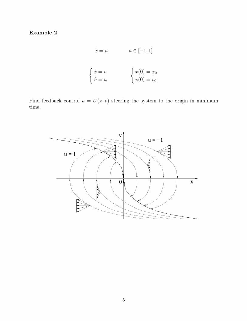
Example 2
x = u u ∈ [−1, 1]
x = v
v = u
x(0) = x0
v(0) = v0
Find feedback control u = U(x, v) steering the system to the origin in minimumtime.
u = 1
0
v
x
u = −1
5

Regularity of Multifunctions
The Hausdorff distance between two compact sets Ω1,Ω2 ⊂ IRn is
dH(Ω1,Ω2).= min
ρ : Ω1 ⊆ B(Ω2, ρ) and Ω2 ⊆ B(Ω1, ρ)
B(Ω, ρ).= neighborhood of radius ρ around the set Ω
Ω2
1ρ
Ω1
ρ
2Ω
1
Ω1B( , )ρ1
Ω1
ρ2
dH(Ω1,Ω2) = maxρ1, ρ2
ρ1 = maximum distance of points p ∈ Ω1 from Ω2
ρ2 = maximum distance of points p ∈ Ω2 from Ω1
A multifunction x 7→ G(x) ⊂ IRn is Lipschitz continuous if
dH(G(x), G(y)
)≤ L |x− y| x, y ∈ IRn.
If U ⊂ IRm is compact and f is Lipschitz continuous, then the multifunction
x 7→ G(x).=f(x, u) ; u ∈ U
is Lipschitz continuous
6

Equivalence with Differential Inclusions
Control System: x = f(x, u) u ∈ U (1)
Differential Inclusion: x ∈ G(x) (2)
F(x) = f(x,u) ; u UC
F(x)
Ux
x
Theorem 1 (A. Filippov). If f is continuous and U is compact, the set of(Caratheodory) trajectories of (1) coincides with the set of trajectories of (2), with
G(x).=f(x, u) ; u ∈ U
If x(t) ∈ G(x(t)
)a.e., for each fixed t there exists u(t) ∈ U such that x(t) =
f(x(t), u(t)
). The map t 7→ u(t) can be chosen to be measurable.
Theorem 2 (A. Ornelas). Let x 7→ G(x) be a bounded, Lipschitz continuousmultifunction with convex, compact values. Then there exists a Lipschitz continuousfunction f : IRn ×U 7→ IRn such that G(x)
.=f(x, u) ; u ∈ U
for all x. Here the
U (the set of control values) is the closed unit ball in IRn.
7

Dynamics of a Control System
• Describe the set of all trajectories of the control system
x = f(x, u) u ∈ U, x(0) = x0 (1)
• Describe the Reachable set at time T:
R(T ).=x(T ) ; x(·) is a trajectory of (1)
R(T)
x0
Ideal case: an explicit formula for R(T )
More realistic goal: derive properties of the reachable set
• A priori bounds: R(T ) ⊂ B(x0, ρ)
• Is R(T ) closed, connected, with non-empty interior ?
• (Local controllability) Is R(T ) a neighborhood of x0, for all T > 0 ?
• (Global controllability) Does every point x ∈ IRn lie in the reachable set R(T ),for T suitably large?
8

Linear Systems
x = Ax+Bu, x(0) = 0 (4)
A is a n× n matrix, B is n×m, u ∈ IRm.
x(T ) =
∫ T
0
e(T−s)ABu(s) ds (5)
etA =
∞∑
k=0
tkAk
k!
Theorem 3. For every T > 0, the reachable set is
R(T ) = spanB, AB,A2B, · · · , An−1B
Proof. R(T ) is clearly a vector space
range(etA)⊆ spanI, A,A2, . . . = span
I, A,A2, . . . An−1
Hence, by (5), R(T ) ⊆ spanB, AB,A2B, · · · , An−1B
.
Viceversa, p ∈ R(T )⊥ implies
⟨p ,
dxk(t)
dt
⟩= 0 for all k, t ≥ 0.
At time t = 0, taking a constant control u(t) ≡ ω, one finds⟨p, AkBω
⟩= 0 for all k ≥ 0, ω ∈ IRm
p ∈ spanB,AB,A2B, . . . An−1B⊥
9
Connectedness
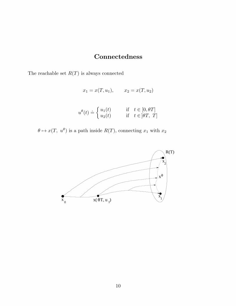
The reachable set R(T ) is always connected
x1 = x(T, u1), x2 = x(T, u2)
uθ(t).=
u1(t) if t ∈ [0, θT ]u2(t) if t ∈ ]θT, T ]
θ 7→ x(T, uθ) is a path inside R(T ), connecting x1 with x2
2
x0
R(T)
x
x1
θ
x( T, u )1θ
x
10
Closure
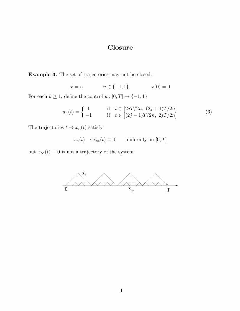
Example 3. The set of trajectories may not be closed.
x = u u ∈ −1, 1, x(0) = 0
For each k ≥ 1, define the control u : [0, T ] 7→ −1, 1
un(t) =
1 if t ∈
[2jT/2n, (2j + 1)T/2n
]
−1 if t ∈[(2j − 1)T/2n, 2jT/2n
] (6)
The trajectories t 7→ xn(t) satisfy
xn(t) → x∞(t) ≡ 0 uniformly on [0, T ]
but x∞(t) ≡ 0 is not a trajectory of the system.
8
320 x
x
T
11

Example 4. The reachable set R(T ) ⊂ IR2 may not be closed.
(x1, x2) = (u, x21) u ∈ −1, 1, (x1, x2)(0) = (0, 0) (7)
Choosing the controls un(·) in (6), at time T we reach the points
Pn =(0, T 3/12n2
)
Pn → (0, 0) as n → ∞, but (0, 0) /∈ R(T ). Indeed, for any trajectory of thesystem
x2(T ) =
∫ T
0
x21(s) ds = 0
only if x1(t) ≡ 0 for all t, hence x1(t) = u(t) = 0 for almost every t. Against theassumption u(t) ∈ −1, 1
0 1 2− 1
0
x
x 1
2
nP
12
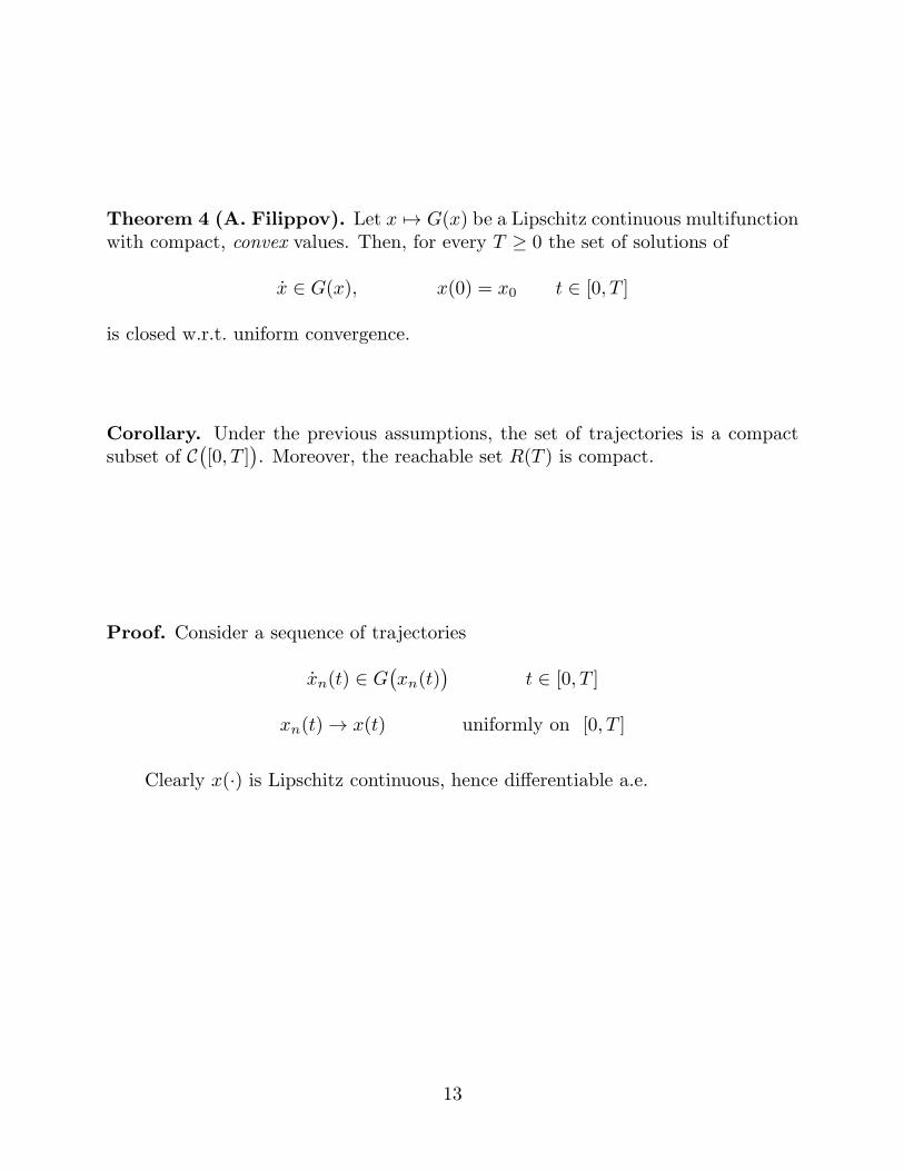
Theorem 4 (A. Filippov). Let x 7→ G(x) be a Lipschitz continuous multifunctionwith compact, convex values. Then, for every T ≥ 0 the set of solutions of
x ∈ G(x), x(0) = x0 t ∈ [0, T ]
is closed w.r.t. uniform convergence.
Corollary. Under the previous assumptions, the set of trajectories is a compactsubset of C
([0, T ]
). Moreover, the reachable set R(T ) is compact.
Proof. Consider a sequence of trajectories
xn(t) ∈ G(xn(t)
)t ∈ [0, T ]
xn(t) → x(t) uniformly on [0, T ]
Clearly x(·) is Lipschitz continuous, hence differentiable a.e.
13

Assume x(t) /∈ G(x(t)
)at some time t. Then x(t) is separated by a hyperplane
from the convex set G(x(t)
)
⟨p , x(t)
⟩≥ 3δ + max
ω∈G(x(t))
⟨p , ω
⟩
⟨p,
x(t+ εt)− x(t)
ε
⟩≥ 2δ + max
ω∈G(x(t))
⟨p , ω
⟩(8)
G(x(t))
x(t)
δ3
G(x(t))
p.x(t)
On the other hand, by continuity of G,
maxω∈G(y)
⟨p , ω
⟩≤ δ + max
ω∈G(x(t))
⟨p , ω
⟩
for∣∣y − x(t)
∣∣ ≤ ρ small. Hence
⟨p,
xn(t+ εt)− xn(t)
ε
⟩≤ max
ω∈G(y), |y−x(t)|≤ρ
⟨p , ω
⟩≤ δ + max
ω∈G(x(t))
⟨p , ω
⟩
Letting n→ ∞, we obtain
⟨p,
x(t+ εt)− x(t)
ε
⟩≤ δ + max
ω∈G(x(t))
⟨p , ω
⟩(9)
in contradiction with (8).
14

Convex Closure and Extreme Points
Let Ω ⊂ IRn be any compact setThe convex closure of Ω, written coΩ, is the smallest closed convex set whichcontains Ω. It admits the representation
coΩ =
n∑
i=0
θiωi ωi ∈ Ω, θi ≥ 0,∑
θi = 1
Hence, if Ω ⊂ IRn, the convex closure coΩ coincides with the set of all convexcombinations of n+ 1 elements of Ω.
ω ω
ωω
ω1
2
34
ω5
6
ω
A point ω ∈ Ω is an extreme point if it CANNOT be written as a convexcombination
ω =
k∑
i=1
θiωi, θi ∈ [0, 1],∑
θi = 1, ωi ∈ Ω, ωi 6= ω
The set of extreme points is written as extΩ
15

ΩΩ co Ωext
Ω ⊂ IRn compact =⇒ extΩ ⊆ Ω ⊆ coΩ = co(extΩ
)
Density Theorems
Let x 7→ G(x) be a multifunction with compact values.We compare the solutions of the differential inclusions
x ∈ extG(x) (10)
x ∈ G(x) (11)
x ∈ coG(x) (12)
Theorem 5 (Relaxation). Let the multifunction x 7→ G(x) be Lipschitz contin-uous with compact values. Then set of trajectories of (10) is dense on the set oftrajectories of (12)
16
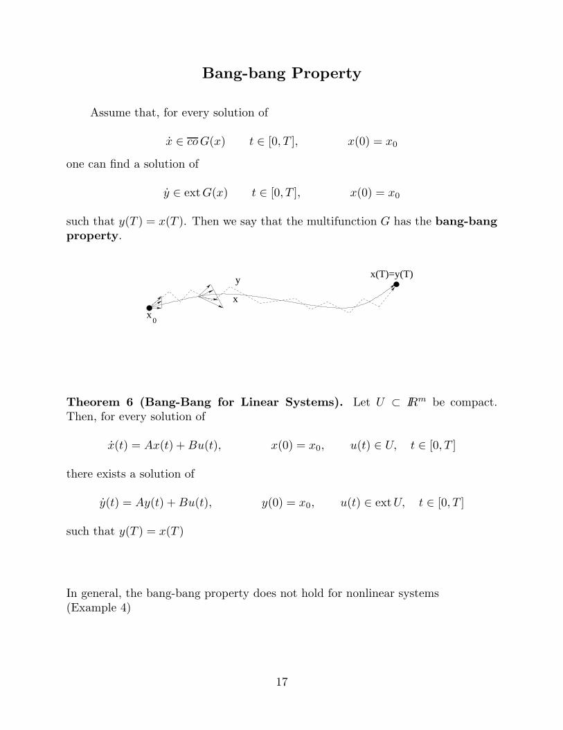
Bang-bang Property
Assume that, for every solution of
x ∈ coG(x) t ∈ [0, T ], x(0) = x0
one can find a solution of
y ∈ extG(x) t ∈ [0, T ], x(0) = x0
such that y(T ) = x(T ). Then we say that the multifunction G has the bang-bangproperty.
x
x0
x(T)=y(T)y
Theorem 6 (Bang-Bang for Linear Systems). Let U ⊂ IRm be compact.Then, for every solution of
x(t) = Ax(t) +Bu(t), x(0) = x0, u(t) ∈ U, t ∈ [0, T ]
there exists a solution of
y(t) = Ay(t) +Bu(t), y(0) = x0, u(t) ∈ extU, t ∈ [0, T ]
such that y(T ) = x(T )
In general, the bang-bang property does not hold for nonlinear systems(Example 4)
17

A Lyapunov-type Convexity Theorem
f1, . . . , fN ∈ L1([0, T ] ; IRn
)
consider a pointwise convex combination of the fi
f(t).=
N∑
i=1
θi(t)fi(t)
θ1, . . . , θN : [0, T ] 7→ [0, 1],∑
θi(t) = 1 for all t
f2
f1
f
1
2
J2
f
0 T T0
f~
Theorem 7. There exists a partition
[0, T ] =
N⋃
i=1
Ji, Ji ∩ Jk = 0 if i 6= k
such that ∫ T
0
f(t) dt =
N∑
i=1
∫
Ji
fi(t) dt
18

Proof of Theorem 7. Consider the set of coefficients of convex combinations
Γ.=
(w1, . . . wN ) ; wi(t) ∈ [0, 1],
N∑
i=1
wi(t) = 1,
∫ T
0
∑
i
wi(t)fi(t) dt =
∫ T
0
f(t) dt
1. Γ is non-empty, because (θ1, . . . , θN ) ∈ Γ
2. Γ ⊂ L∞ is closed and convex, hence compact in a weak topology
3. By the Krein-Milman Theorem, Γ has an extreme point (w∗1 , . . . , w
∗n)
4. By extremality, the functions w∗i : [0, T ] 7→ [0, 1] actually take values in 0, 1
5. Take Ji =t ∈ [0, T ] ; w∗
i (t) = 1
Proof of Theorem 6.
Consider any control u : [0, T ] 7→ U ⊂ IRm. Then
u(t) =
m∑
i=0
θi(t)ui(t) ui(t) ∈ extU
Using the control u(·), the terminal point is
x(T ) =
∫ T
0
e(T−s)ABu(s) ds =
∫ T
0
m∑
i=0
θi(t)e(T−s)ABui(s) ds
Apply previous theorem with fi(s) = e(T−s)ABui(s). For a suitable partition[0, T ] = J0 ∪ J1 ∪ · · · ∪ Jm, one has
x(T ) =
m∑
i=0
∫
Ji
e(T−s)ABui(s) ds
Hence the controlu∗(t) = ui(t) if t ∈ Ji
takes values in extU and reaches exactly the same terminal point x(T ).
19
Baire Category Approach
Baire Category Theorem. Let K be a complete metric space, (Kn)n≥1 a se-quence of open, dense subsets. Then
⋂n≥1Kn is non-empty and dense in K.
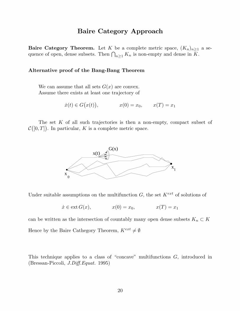
Alternative proof of the Bang-Bang Theorem
We can assume that all sets G(x) are convex.Assume there exists at least one trajectory of
x(t) ∈ G(x(t)
), x(0) = x0, x(T ) = x1
The set K of all such trajectories is then a non-empty, compact subset ofC([0, T ]
). In particular, K is a complete metric space.
x(t)G(x)
x0
x1
Under suitable assumptions on the multifunction G, the set Kext of solutions of
x ∈ extG(x), x(0) = x0, x(T ) = x1
can be written as the intersection of countably many open dense subsets Kn ⊂ K
Hence by the Baire Cathegory Theorem, Kext 6= ∅
This technique applies to a class of “concave” multifunctions G, introduced in(Bressan-Piccoli, J.Diff.Equat. 1995)
20

1. For each compact, convex set Ω ⊂ IRn, define the function ϕΩ : Ω 7→ [0,∞[ as
ϕΩ(p).= sup
(∫ 1
0
∣∣X(s)− p∣∣2 ds
)1/2
; X : [0, 1] 7→ Ω,
∫ 1
0
X(s) ds = p
Observe that ϕ2Ω(p) is the maximum variance among all random variables X taking
values inside Ω, whose expected value is E[X] = p.
2. Each function ϕΩ is ≥ 0, concave, continuous and ϕΩ(p) = 0 iff p ∈ extΩ
3. The functional
Φ(x(·)
) .=
∫ T
0
ϕG(x)
(x(t)
)dt
is well defined for all trajectories of x ∈ G(x)Moreover Φ
(x(·)
)= 0 iff x(t) ∈ extG
(x(t)
)for a.e. t ∈ [0, T ]
4. The sets Kn.=x(·) ∈ K ; Φ(x) < 1/n
are open and dense in K
5. By the Baire Cathegory Theorem, Kext =⋂
n≥1Kn 6= ∅.
This shows that, (in a topological sense) “almost all” solutions of x ∈ G(x) areactually solutions of x ∈ extG(x).
p
ϕ
Ω
Ω(p)
21
Chattering Controls
Given a control system on IRn
x = f(x, u) u ∈ U (1)
for each x, the set of velocities
G(x).=f(x, u) ; u ∈ U
may not be convex. We seek a new control system
x = f(x, u) u ∈ U (13)
such thatG(x)
.=f(x, u) ; u ∈ U
= coG(x)
Since every ω ∈ coG(x) is a convex combination of n + 1 vectors in G(x), thesystem (13) can be defined as follows:
∆.=
(θ0, θ1, . . . , θn) ; θi ∈ [0, 1],
n∑
i=0
θi = 1
U.= U × · · · × U ×∆
(n+1 times)
f(x, u) = f(x, u1, . . . , un, θ0, . . . , θn) =
n∑
i=0
θif(x, ui) (14)
The system (14) is called a chattering system
A control u = (u0, . . . , un, θ0, . . . , θn) ∈ U is called a chattering control
• The set of trajectories of a chattering system is always closed in C([0, T ]
)
• The reachable set R(T ) is compact.
• Every trajectory of (13) can be uniformly approximated by trajectories of theoriginal system (1)
22
Lie Brackets
Given two smooth vector fields f, g, their Lie bracket is defined as
[f, g].= (Dg) · f − (Df) · g
In other words, [f, g] is the directional derivative of g in the direction of fminus the directional derivative of f in the direction of g.
Exponential notation for the flow map:τ 7→ (exp τf)(x) denotes the solution of the Cauchy problem
dw
dτ= f(w), w(0) = x
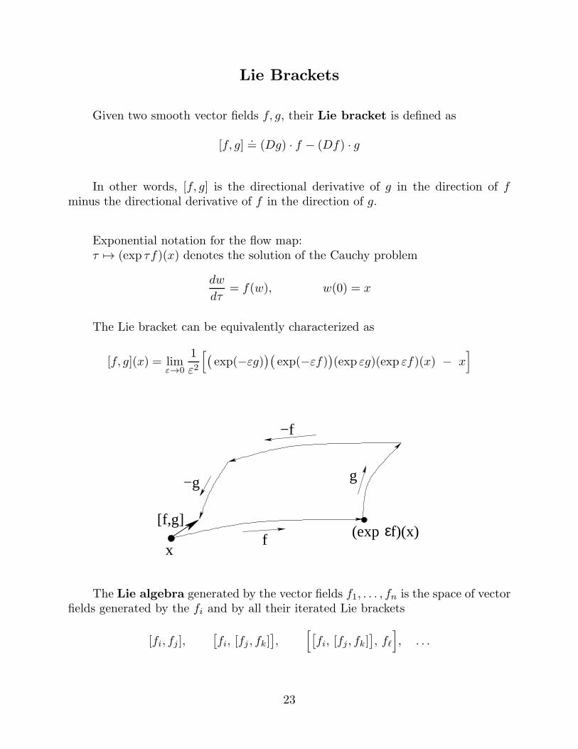
The Lie bracket can be equivalently characterized as
[f, g](x) = limε→0
1
ε2
[(exp(−εg)
)(exp(−εf)
)(exp εg)(exp εf)(x) − x
]
[f,g]f
−f
−g g
x(exp f)(x)ε
The Lie algebra generated by the vector fields f1, . . . , fn is the space of vectorfields generated by the fi and by all their iterated Lie brackets
[fi, fj ],[fi, [fj , fk]
],
[[fi, [fj , fk]
], fℓ
], . . .
23
Local Controllability
x =
m∑
i=1
fi(x)ui ui ∈ [−1, 1] (15)
x(0) = x0 ∈ IRn
Theorem 8. If the linear span of all iterated Lie brackets of f1, . . . , fn at x0 is thewhole space IRn, then the system (15) is locally controllable.That means: for every T > 0 the reachable set R(T ) is a neighborhood of x0.
More difficult case: a drift f0 is present.
x = f0(x) +m∑
i=1
fi(x)ui ui ∈ [−1, 1] (16)
Theorem 9 (Sussmann-Jurdjevic). If the linear span of all iterated Lie bracketsof f0, f1, . . . , fn at x0 is the whole space IRn, then for every T > 0 the set of pointsreachable within time ≤ T has non-empty interior.
Local controllability for (16) is a hard problem!
24
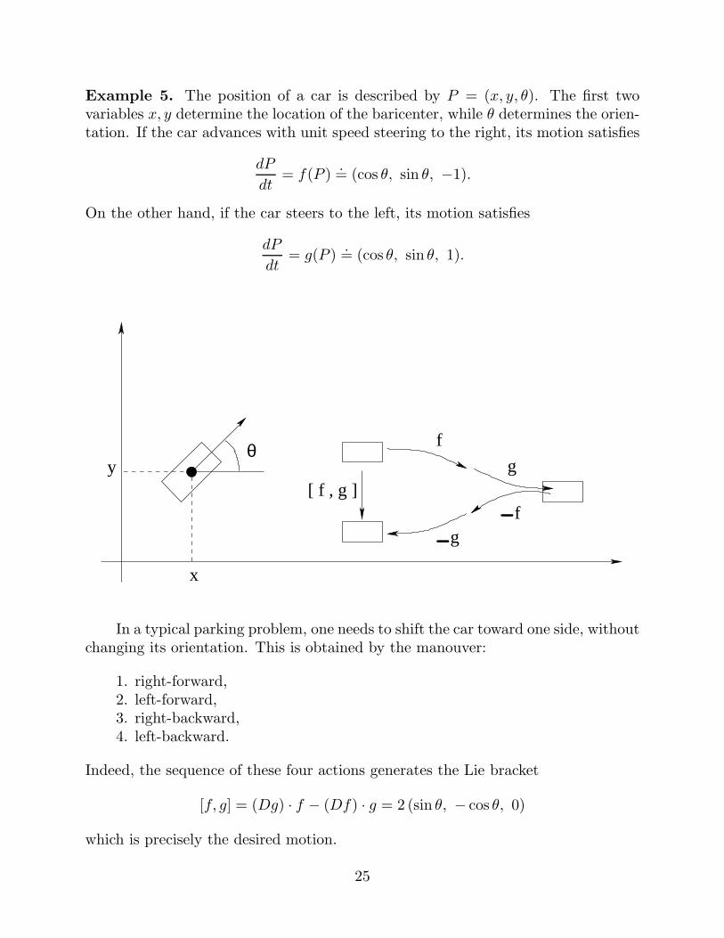
Example 5. The position of a car is described by P = (x, y, θ). The first twovariables x, y determine the location of the baricenter, while θ determines the orien-tation. If the car advances with unit speed steering to the right, its motion satisfies
dP
dt= f(P )
.= (cos θ, sin θ, −1).
On the other hand, if the car steers to the left, its motion satisfies
dP
dt= g(P )
.= (cos θ, sin θ, 1).
yθ f
fg
g
−−
[ f , g ]
x
In a typical parking problem, one needs to shift the car toward one side, withoutchanging its orientation. This is obtained by the manouver:
1. right-forward,2. left-forward,3. right-backward,4. left-backward.
Indeed, the sequence of these four actions generates the Lie bracket
[f, g] = (Dg) · f − (Df) · g = 2 (sin θ, − cos θ, 0)
which is precisely the desired motion.
25
The system on IR3
P = f(P )u1 + g(P )u2, u1, u2 ∈ [−1, 1]
is locally controllable. Indeed,
spanf(P ), g(P ), [f, g](P )
= IR3
because it contains the three vectors (cos θ, sin θ, −1), (cos θ, sin θ, −1) and(sin θ, − cos θ, 0)
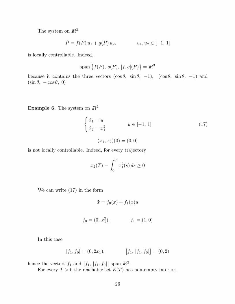
Example 6. The system on IR2
x1 = u
x2 = x21u ∈ [−1, 1] (17)
(x1, x2)(0) = (0, 0)
is not locally controllable. Indeed, for every trajectory
x2(T ) =
∫ T
0
x21(s) ds ≥ 0
We can write (17) in the form
x = f0(x) + f1(x)u
f0 = (0, x21), f1 = (1, 0)
In this case
[f1, f0] = (0, 2x1),[f1, [f1, f0]
]= (0, 2)
hence the vectors f1 and[f1, [f1, f0]
]span IR2.
For every T > 0 the reachable set R(T ) has non-empty interior.
26

Optimal Control Problems
x = f(x, u) u ∈ U, t ∈ [0, T ] (1)
x(0) = x0 ∈ IRn (2)
Among all trajectories of (1)-(2), we seek one which is optimal w.r.t. some costcriterion:
Mayer Problem
minimize J = ψ(x(T )
)(18)
Lagrange Problem
minimize J =
∫ T
0
ϕ(t, x(t), u(t)
)dt (19)
Bolza Problem
minimize J =
∫ T
0
ϕ(t, x(t), u(t)
)dt+ ψ
(x(T )
)(20)
ϕ(x, u) = running cost per unit timeψ(x) = terminal cost
27

The minimization is always performed among all control functions u : [0, T ] 7→ U
One may also add a terminal constraint, requiring
x(T ) ∈ S (21)
for some set S ⊂ IRn
Basic assumptions: The cost functions ϕ, ψ are continuous. The set S is closed.
Equivalence of various formulations
1. A Mayer Problem can be written as a Lagrange Problem, taking
ϕ(x, u).= ∇ψ(x) · f(x, u)
We are then minimizing
∫ T
0
∇ψ(x(t)
)· f(x(t), u(t)
)dt =
∫ T
0
∇ψ(x(t)
)· x(t) dt
=
∫ T
0
(d
dtψ(x(t)
))dt = ψ
(x(T )
)− ψ
(x0)
2. A Lagrange Problem can be written as a Mayer Problem, introducing a newvariable xn+1 with
xn+1(0) = 0, xn+1 = ϕ(t, x(t), u(t)
)
and definingψ(x)
.= xn+1
This yields the terminal cost
ψ(x(T )
)= xn+1(T ) =
∫ T
0
ϕ(t, x(t), u(t)
)dt
28

Relations with the Calculus of Variations
Standard Problem in the Calculus of Variations
minimize
∫ T
0
L(t, x(t), x(t)
)dt (22)
among all absolutely continuous functions x : [0, T ] 7→ IRn with
x(0) = x0, x(T ) = x1
Optimal Control Problem
minimize
∫ T
0
ϕ(t, x(t), u(t)
)dt (19)
x = f(x, u) u ∈ U, t ∈ [0, T ] (1)
x(0) = x0, x(T ) = x1 (2)
1. We can write (22) as an optimal control problem by setting
x = u, u ∈ U.= IRn
ϕ(t, x, u).= L(t, x, u)
2. We can write (19) in the form (22) by setting
L(t, x, p).= min
ϕ(t, x, u) ; u ∈ U, f(x, u) = p
L(t, x, p) = ∞ if p /∈f(x, u) ;u ∈ U
L(t, x, p) is the minimum running cost, among all controls that yield the speedx(t) = p.
29

Existence of Optimal Controls
Mayer problem:
minimize J = ψ(x(T )
)(18)
for the systemx = f(x, u), u ∈ U (1)
with constraintsx(0) = x0, x(T ) ∈ S (2)
x0
S
R(T)
30

Theorem 10 (Existence for Mayer Problem).Assume that, for each x, the set of velocities
G(x).=f(x, u) ; u ∈ U
is convex. If there exists at least one trajectory x(·) that satisfies (1)-(2), then theMayer problem (18) admits an optimal solution.
Proof. By Theorem 4, the reachable set R(T ) is compact.
By the assumptions, R(T ) ∩ S is non-empty and compact.
The continuous function ψ admits a global minimum on the compact set R(T )∩S.This yields the optimal solution.
Bolza Problem:
minimize J =
∫ T
0
ϕ(t, x(t), u(t)
)dt+ ψ
(x(T )
)(20)
for the system (1) with initial and terminal conditions (2).
Theorem 11 (Existence for the Bolza Problem). Assume that, for every t, x,the set
G+(t, x).=(y, yn+1) ∈ IRn+1 ; y = f(x, u), yn+1 ≥ ϕ(t, x, u) for some u ∈ U
is convex. If there exists at least one trajectory x(·) that satisfies (1)-(2), then theBolza problem (20) admits an optimal solution.
31

Remark: For the problem:
minimize
∫ T
0
L(t, x(t), u(t)
)dt (22)
subject tox = u, x(0) = x0, x(T ) = x1
corresponding to the standard problem in the Calculus of Variations, the set
G+(t, x).=(y, yn+1) ∈ IRn+1 ; y = f(x, u), yn+1 ≥ ϕ(t, x, u) for some u ∈ U
=(u, yn+1) ∈ IRn+1 ; yn+1 ≥ L(t, x, u)
is precisely the epigraph of the function u 7→ L(t, x, u)This is a convex set iff L(t, x, x) is convex as a function of x
L(t, x, x).
.x
32
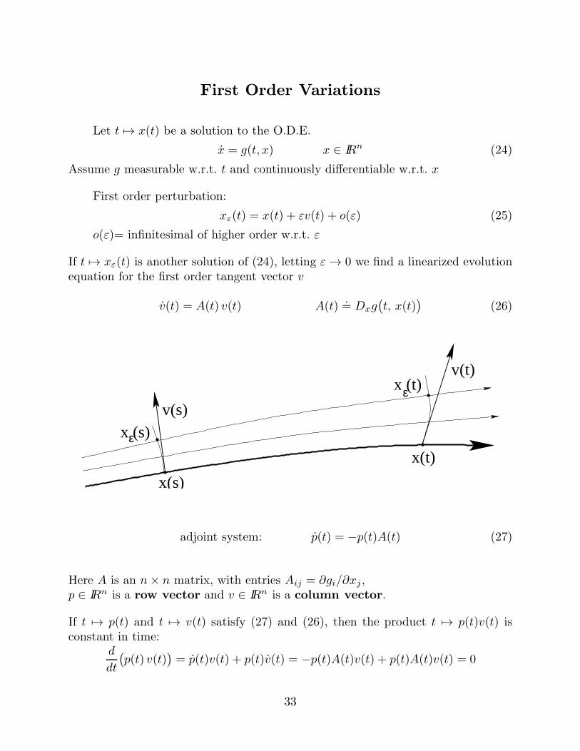
First Order Variations
Let t 7→ x(t) be a solution to the O.D.E.
x = g(t, x) x ∈ IRn (24)
Assume g measurable w.r.t. t and continuously differentiable w.r.t. x
First order perturbation:
xε(t) = x(t) + εv(t) + o(ε) (25)
o(ε)= infinitesimal of higher order w.r.t. ε
If t 7→ xε(t) is another solution of (24), letting ε→ 0 we find a linearized evolutionequation for the first order tangent vector v
v(t) = A(t) v(t) A(t).= Dxg
(t, x(t)
)(26)
v(s)
v(t)
x(t)
x(s)
x (s)ε
εx (t)
adjoint system: p(t) = −p(t)A(t) (27)
Here A is an n× n matrix, with entries Aij = ∂gi/∂xj ,p ∈ IRn is a row vector and v ∈ IRn is a column vector.
If t 7→ p(t) and t 7→ v(t) satisfy (27) and (26), then the product t 7→ p(t)v(t) isconstant in time:
d
dt
(p(t) v(t)
)= p(t)v(t) + p(t)v(t) = −p(t)A(t)v(t) + p(t)A(t)v(t) = 0
33

Necessary Conditions for Optimality
x = f(x, u) t ∈ [0, T ], x(0) = x0 (28)
Family of admissible control functions: U .=u : [0, T ] 7→ U
For u(·) ∈ U , the trajectory of (28) is t 7→ x(t, u)
Mayer problem, free terminal point:
maxu∈U
ψ(x(T, u)
)(29)
ψ = ψ
x0
R(T)
x*
max
34
Assume: t 7→ u∗(t) is an optimal controlt 7→ x∗(t) = x
(t, u∗(t)
)is the corresponding optimal trajectory.
The value ψ(x(T, u∗)
)cannot be increased by any perturbation of the control u∗(·).
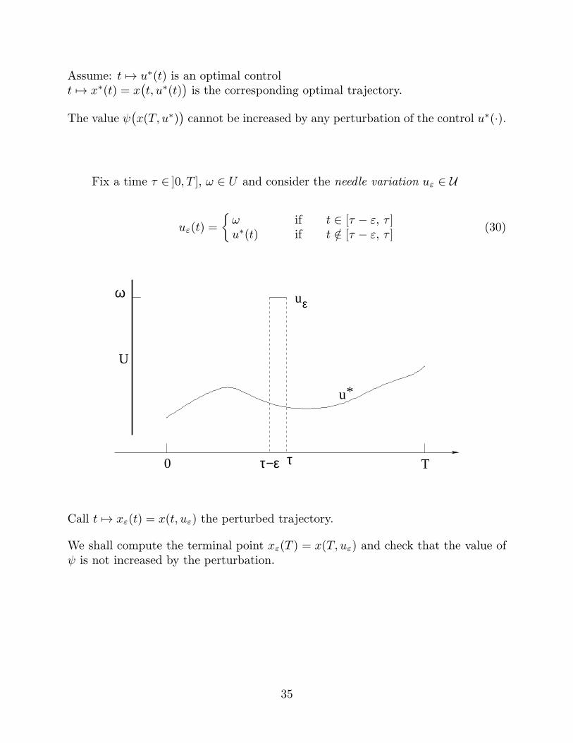
Fix a time τ ∈ ]0, T ], ω ∈ U and consider the needle variation uε ∈ U
uε(t) =
ω if t ∈ [τ − ε, τ ]u∗(t) if t /∈ [τ − ε, τ ]
(30)
U
ω
0 T
u*
uε
τ−ε τ
Call t 7→ xε(t) = x(t, uε) the perturbed trajectory.
We shall compute the terminal point xε(T ) = x(T, uε) and check that the value ofψ is not increased by the perturbation.
35
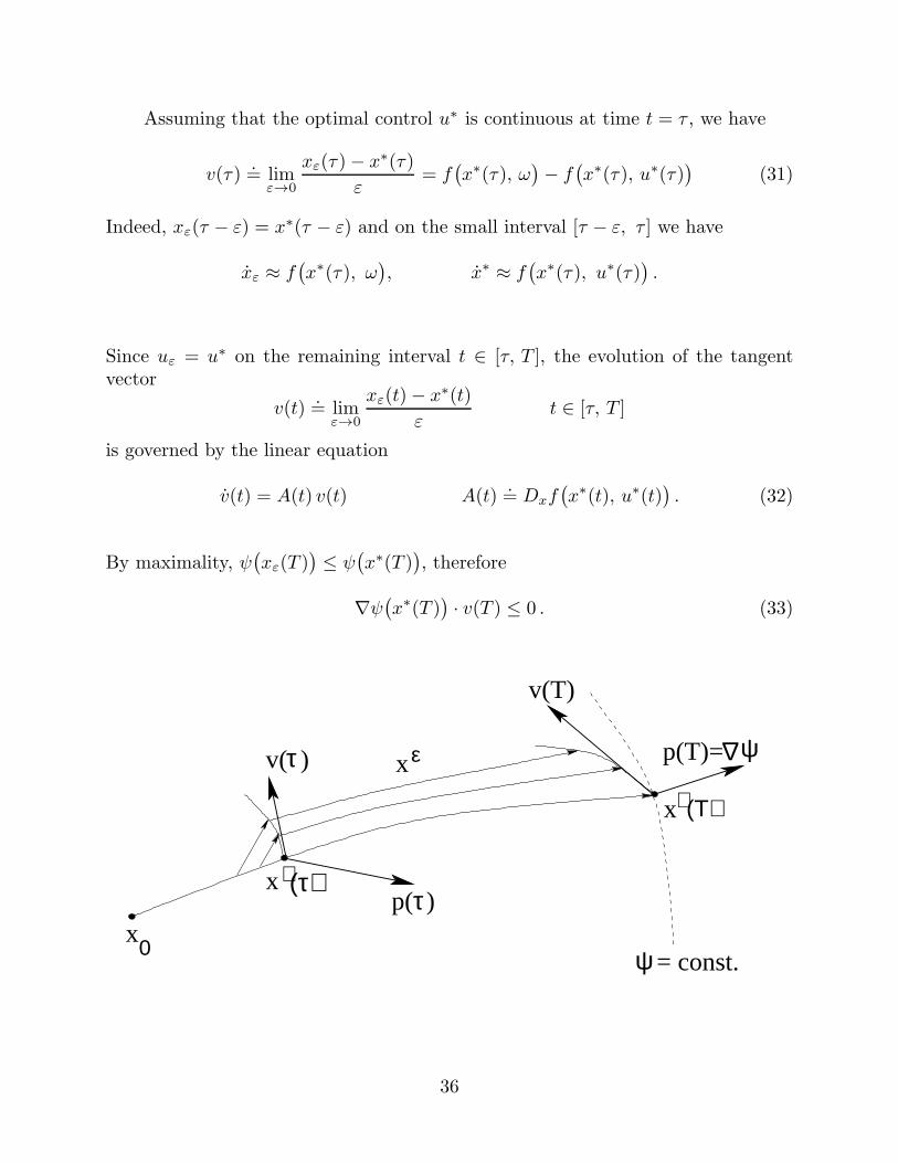
Assuming that the optimal control u∗ is continuous at time t = τ , we have
v(τ).= lim
ε→0
xε(τ)− x∗(τ)
ε= f
(x∗(τ), ω
)− f
(x∗(τ), u∗(τ)
)(31)
Indeed, xε(τ − ε) = x∗(τ − ε) and on the small interval [τ − ε, τ ] we have
xε ≈ f(x∗(τ), ω
), x∗ ≈ f
(x∗(τ), u∗(τ)
).
Since uε = u∗ on the remaining interval t ∈ [τ, T ], the evolution of the tangentvector
v(t).= lim
ε→0
xε(t)− x∗(t)
εt ∈ [τ, T ]
is governed by the linear equation
v(t) = A(t) v(t) A(t).= Dxf
(x∗(t), u∗(t)
). (32)
By maximality, ψ(xε(T )
)≤ ψ
(x∗(T )
), therefore
∇ψ(x∗(T )
)· v(T ) ≤ 0 . (33)
x ∗ (τ)
∗x (Τ)
x0
τ
p( )τ
v(T)
∆ψp(T)= xε
ψ= const.
v( )
36
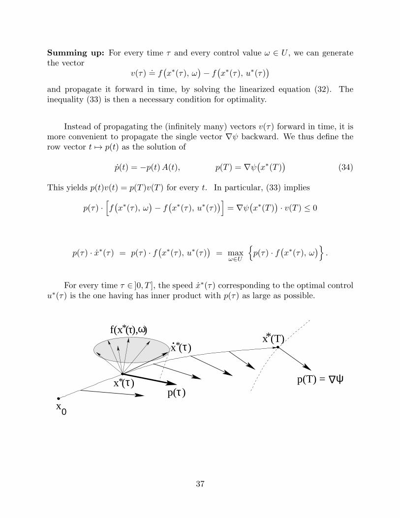
Summing up: For every time τ and every control value ω ∈ U , we can generatethe vector
v(τ).= f
(x∗(τ), ω
)− f
(x∗(τ), u∗(τ)
)
and propagate it forward in time, by solving the linearized equation (32). Theinequality (33) is then a necessary condition for optimality.
Instead of propagating the (infinitely many) vectors v(τ) forward in time, it ismore convenient to propagate the single vector ∇ψ backward. We thus define therow vector t 7→ p(t) as the solution of
p(t) = −p(t)A(t), p(T ) = ∇ψ(x∗(T )
)(34)
This yields p(t)v(t) = p(T )v(T ) for every t. In particular, (33) implies
p(τ) ·[f(x∗(τ), ω
)− f
(x∗(τ), u∗(τ)
)]= ∇ψ
(x∗(T )
)· v(T ) ≤ 0
p(τ) · x∗(τ) = p(τ) · f(x∗(τ), u∗(τ)
)= max
ω∈U
p(τ) · f
(x∗(τ), ω
).
For every time τ ∈ ]0, T ], the speed x∗(τ) corresponding to the optimal controlu∗(τ) is the one having has inner product with p(τ) as large as possible.
* τ
*
*.
p(T) =
f(x ( ), )ω
0
p( )τ
*
ψ∆x ( )τ
x ( )τx (T)
x
37
Pontryagin Maximum Principle (Mayer Problem, free terminal point)
Consider the control system
x = f(x, u) u(t) ∈ U t ∈ [0, T ] (35)
with initial datax(0) = x0 . (36)
Let t 7→ u∗(t) be an optimal control and t 7→ x∗(t) = x(t, u∗) be the optimaltrajectory for the maximization problem
maxu∈U
ψ(x(T, u)
). (37)
Define the vector t 7→ p(t) as the solution to the linear adjoint system
p(t) = −p(t)A(t), A(t).= Dxf
(x∗(t), u∗(t)
)(38)
with terminal conditionp(T ) = ∇ψ
(x∗(T )
). (39)
Then, for almost every τ ∈ [0, T ] the following maximality condition holds
p(τ) · f(x∗(τ), u∗(τ)
)= max
ω∈U
p(τ) · f
(x∗(τ), ω
)(39)
38

Computing the Optimal Control
STEP 1: solve the pointwise maximixation problem (39), obtaining the optimalcontrol u∗ as a function of p, x, i.e.
u∗(x, p) = argmaxω∈U
p · f(x, ω)
(40)
STEP 2: solve the two-point boundary value problem
x = f
(x, u∗(x, p)
)
p = −p ·Dxf(x, u∗(x, p)
)x(0) = x0
p(T ) = ∇ψ(x(T )
) (41)
• In general, the function u∗ = u∗(p, x) in (40) is highly nonlinear. It may bemultivalued or discontinuous.
• The two-point boundary value problem (41) can be solved by a shooting method:Guess an initial value p(0) = p0 and solve the corresponding Cauchy problem.Try to adjust the value of p0 so that the terminal values x(T ), p(T ) satisfy thegiven conditions.
39

Example 1 (Linear pendulum).
q(t) = position of a linearized pendulum, controlled by an external force with mag-nitude u(t) ∈ [−1, 1].
q(t) + q(t) = u(t), q(0) = q(0) = 0, u(t) ∈ [−1, 1]
We wish to maximize the terminal displacement q(T ).
Equivalent control system: x1 = q, x2 = q
x1 = x2
x2 = u− x1
x1(0) = 0
x2(0) = 0
maximize x1(T ) over all controls u : [0, T ] 7→ [−1, 1]
Let t 7→ x∗(t) = x(t, u∗) be an optimal trajectory. The linearized equation fora tangent vector is (
v1v2
)=
(0 1−1 0
)(v1v2
)
The corresponding adjoint vector p = (p1, p2) satisfies
(p1, p2) = −(p1, p2)
(0 1−1 0
), (p1, p2)(T ) = ∇ψ
(x∗(T )
)= (1, 0) (42)
because ψ(x).= x1.
In this special linear case, we can explicitly solve (42) without needing to knowx∗, u∗. An easy computation yields
(p1, p2)(t) =(cos(T − t), sin(T − t)
)(43)
40
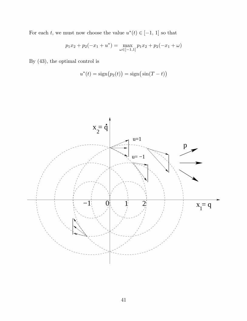
For each t, we must now choose the value u∗(t) ∈ [−1, 1] so that
p1x2 + p2(−x1 + u∗) = maxω∈[−1,1]
p1x2 + p2(−x1 + ω)
By (43), the optimal control is
u∗(t) = sign(p2(t)
)= sign
(sin(T − t)
)
.
u=1
u= −1
x = q
x = q1
2
p
0 1 2−1
41
Example 2. Consider the problem on IR3
maximize x3(T ) over all controls u : [0, T ] 7→ [−1, 1]
for the system
x1 = u
x2 = −x1x3 = x2 − x21
x1(0) = 0
x2(0) = 0
x3(0) = 0
The adjoint equations take the form
(p1, p2, p3) = (p2 + 2x1p3, −p3, 0) (p1, p2, p3)(T ) = (0, 0, 1) (44)
Maximixing the inner product p · x we obtain the optimality conditions for thecontrol u∗
p1u∗ + p2 (−x1) + p3 (x2 − x21) = max
ω∈[−1,1]p1ω + p2 (−x1) + p3 (x2 − x21) (45)
u∗ = 1 if p1 > 0u∗ ∈ [−1, 1] if p1 = 0u∗ = −1 if p1 < 0
Solving the terminal value problem (44) for p2, p3 we find
p3(t) ≡ 1, p2(t) = T − t
42

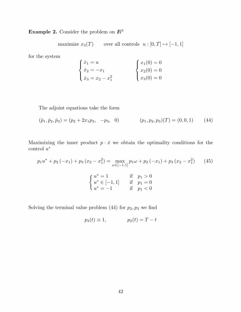
The function p1 can now be found from the equations
p1 = −1 + 2u∗ = −1 + 2 sign(p1), p1(T ) = 0, p1(0) = p2(0) = T
with the convention: sign(0) = [−1, 1]. The only solution is found to be
p1(t) =
−3
2
(T
3− t
)2
if 0 ≤ t ≤ T/3
0 if T/3 ≤ t ≤ T
The optimal control is
u∗(t) =
−1 if 0 ≤ t ≤ T/31/2 if T/3 ≤ t ≤ T
Observe that on the interval [T/3, T ] the optimal control is derived not from themaximality condition (45) but from the equation p1 = (−1 + 2u) ≡ 0. An optimalcontrol with this property is called singular.
Τ
p
0
p = 1
Τ/3
p = −3
1
1
1..
..
43

Tangent Cones
x = f(x, u) u ∈ U, x(0) = x0
Let t 7→ x∗(t) = x(t, u∗) be a reference trajectory.Given τ ∈ ]0, T ], ω ∈ U , consider the family of needle variations
uε(t) =
ω if t ∈ [τ − ε, τ ]u∗(t) if t /∈ [τ − ε, τ ]
(30)
Call vτ,ω(T ).= lim
ε→0
x(T, uε)− x(T, u∗)
ε
the first order variation of the terminal point of the corresponding trajectory.
Define Γ as the smallest convex cone containing all vectors vτ,ω
This is a cone of feasible directions, i.e. directions in which we can move theterminal point x(T, u∗) by suitably perturbing the control u∗.
x 0
R(T)
x (T)
x
x ( )
*
τ
ε
*Γ
44

Consider a terminal constraint x(T ) ∈ S, where
S.=x ∈ IRn ; φi(x) = 0, i = 1, . . . , N
.
Assume that the N + 1 gradients ∇ψ, ∇φ1, . . . ,∇φN are linearly independent atthe point x∗. Then the tangent space to S at x∗ is
TS =v ∈ IRn ; ∇φi(x∗) · v = 0 i = 1, . . . , N
.
The tangent cone to the set
S+ =x ∈ S ; ψ(x) ≥ ψ(x∗)
isTS+ =
v ∈ IRn ; ∇ψ(x∗) · v ≥ 0, ∇φi(x∗) · v = 0 i = 1, . . . , N
When x∗ = x∗(T ), we think of TS+ as the cone of profitable directions,i.e. those directions in which we would like to move the terminal point, in order toincrease the value of ψ and still satisfy the constraint x(T ) ∈ S.
S
S
(x (T))
x (T)
T
*
+
T
S
∆ψ *
Lemma 1. A vector p ∈ IRn satisfies
p · v ≥ 0 for all v ∈ TS+ (46)
if and only if it can be written as a linear combination
p = λ0 ∇ψ(x∗) +N∑
i=1
λi ∇φi(x∗) with λ0 ≥ 0 . (47)
45
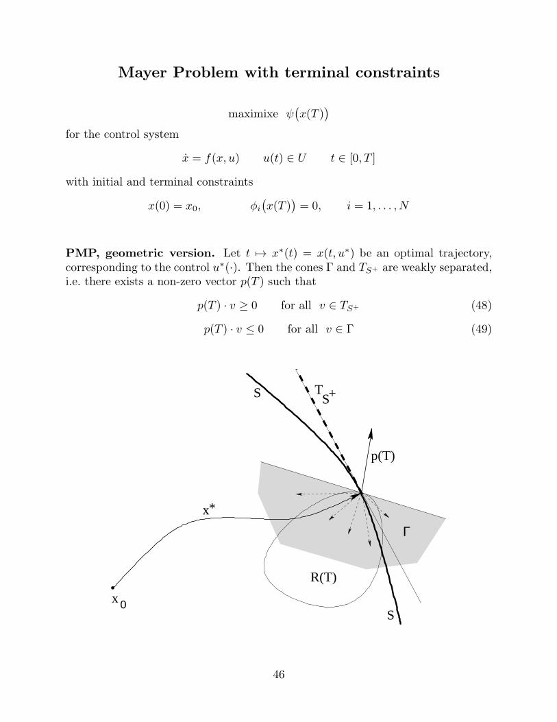
Mayer Problem with terminal constraints
maximixe ψ(x(T )
)
for the control system
x = f(x, u) u(t) ∈ U t ∈ [0, T ]
with initial and terminal constraints
x(0) = x0, φi(x(T )
)= 0, i = 1, . . . , N
PMP, geometric version. Let t 7→ x∗(t) = x(t, u∗) be an optimal trajectory,corresponding to the control u∗(·). Then the cones Γ and TS+ are weakly separated,i.e. there exists a non-zero vector p(T ) such that
p(T ) · v ≥ 0 for all v ∈ TS+ (48)
p(T ) · v ≤ 0 for all v ∈ Γ (49)
x 0
x*
S TS+
p(T)
R(T)
S
Γ
46
PMP, analytic version. Let t 7→ x∗(t) = x(t, u∗) be an optimal trajectory,corresponding to the control u∗(·). Then there exists a non-zero vector functiont 7→ p(t) such that
p(T ) = λ0 ∇ψ(x∗(T )
)+
N∑
i=1
λi ∇φi(x∗(T )
)with λ0 ≥ 0 (50)
p(t) = −p(t)Dxf(x∗(t), u∗(t)
)t ∈ [0, T ] (51)
p(τ) · f(x∗(τ), u∗(τ)
)= max
ω∈U
p(τ) · f
(x∗(τ), ω
)for a.e. τ ∈ [0, T ]. (52)
Indeed, Lemma 1 states that (48) ⇐⇒ (50)
We now show that (49)⇐⇒ (51)+(52).Recall that every tangent vector vτ,ω satisfies the linear evolution equation
vτ,ω(t) = Dxf(x∗(t), u∗(t)
)vτ,ω(t)
If t 7→ p(t) satisfies (51), then the product p(t) · vτ,ω(t) is constant. Hence
p(T ) · vτ,ω(T ) ≤ 0
if and only ifp(τ) · vτ,ω(τ) ≤ 0
if and only if
p(τ) ·[f(x∗(τ), ω
)− f
(x∗(τ), u∗(τ)
)]≤ 0
if and only if (52) holds.
47

High Order Conditions ?
The Pontryagin Maximum Principle is a first order necessary condition.For the Mayer problem
maximize ψ(x(T, u)
)
if u∗(·) is a given control, and if we can find a sequence of perturbed controls uεsuch that
limε→0
ψ(x(T, uε)
)− ψ
(x(T, u∗)
)
‖uε − u∗‖L1
> 0
then the PMP will detect the non-optimality of u∗. However, if the increment inthe value of ψ is of second or higher order w.r.t. the variation ‖uε−u∗‖L1 , then theconclusion of the PMP may still hold, even if u∗ is not optimal.
Example 3.maximize ψ
(x(T )
) .= x2(T )
for the system
(x1, x2) = (u, x21), (x1, x2)(0) = (0, 0), u(t) ∈ [−1, 1].
The constant control u∗(t) ≡ 0 yields the constant trajectory (x∗1, x∗2)(t) ≡ (0, 0).
The corresponding adjoint vector satisfying
(p1, p2) = (−2x1p2, 0) = (0, 0), (p1, p2)(T ) = (0, 1)
is trivially found to be (p1, p2)(t) ≡ (0, 1). Hence the maximality condition
p1u∗ + p2 (x
∗1)
2 = 0 = maxω∈[−1,1]
0 · ω + 1 · 0
is satisfied for every t ∈ [0, T ]. However, the control u∗ ≡ 0 produces the worstpossible outcome. Any other control u 6= u∗ would yield
x2(T, u) =
∫ T
0
(∫ t
0
u(s) ds
)2
dt > x2(T, u∗) = 0.
Notice that in this case the increase in ψ is only of second order w.r.t. the pertur-bation u− u∗
x2(T, u) ≤∫ T
0
(∫ T
0
∣∣u(s)∣∣ ds)2
dt ≤ T · ‖u‖2L1
48

Lagrange Minimization Problem, fixed terminal point
minimize
∫ T
0
L(t, x, u) dt (53)
for the control system on IRn
x = f(t, x, u) u(t) ∈ U (54)
with initial and terminal constraints
x(0) = x0, x(T ) = x♯ (55)
PMP, Lagrange problem.
Let t 7→ x∗(t) = x(t, u∗) be an optimal trajectory, corresponding to the optimalcontrol u∗(·). Then there exist a constant λ0 ≥ 0 and a row vector t 7→ p(t) (notboth = 0) such that
p(t) = −p(t)Dxf(t, x∗(t), u∗(t)
)− λ0DxL
(t, x∗(t), u∗(t)
)(56)
p(t) · f(t, x∗(t), u∗(t)
)+λ0 L
(t, x∗(t), u∗(t)
)
= minω∈U
p(t) · f
(t, x∗(t), ω
)+ λ0 L
(t, x∗(t), ω
).
(57)
This follows by applying the previous results to the Mayer problem
minimize xn+1(T )
withxn+1 = L(t, x, u), xn+1(0) = 0
Because of the terminal constraints (x1, . . . , xn)(T ) = (x♯1, . . . , x♯n), the only require-
ment on the terminal value (p1, . . . , pn, pn+1)(T ) is
pn+1(T ) ≥ 0
Observe that pn+1 = 0, hence pn+1(t) ≡ λ0 for some constant λ0 ≥ 0.
49
Applications to the Calculus of Variations
Standard problem of the Calculus of Variations:
minimize
∫ T
0
L(t, x(t), x(t)
)dt (58)
over all absolutely continuous functions x : [0, T ] 7→ IRn such that
x(0) = x0, x(T ) = x♯ (55)
This corresponds to the optimal control problem (53), for the control system
x = u, u ∈ IRn (59)
We assume that L is smooth, and that x∗(·) is an optimal solution. By thePontryagin Maximum Principle (56)-(57), there exist a constant λ0 ≥ 0 and a rowvector t 7→ p(t) (not both = 0) such that
p(t) = −λ0∂
∂xL(t, x∗(t), x∗(t)
)(60)
p(t) · x∗(t) + λ0 L(t, x∗(t), x∗(t)
)= min
ω∈IRn
p(t) · ω + λ0 L
(t, x∗(t), ω
)(61)
If λ0 = 0, then p(t) 6= 0. But in this case x∗ cannot provide a minimum over thewhole space IRn. This contradiction shows that we must have λ0 > 0.
Since λ0, p are determined up to a positive scalar multiple, we can assume λ0 = 1.
With this choice (61) implies
p(t) = − ∂
∂xL(t, x∗(t), x∗(t)
)(62)
50

The evolution equation
p(t) = − ∂
∂xL(t, x∗(t), x∗(t)
)(60)
now yields the famous Euler-Lagrange equations
d
dt
[∂
∂xL(t, x∗(t), x∗(t)
)]=
∂
∂xL(t, x∗(t), x∗(t)
). (63)
Moreover, the minimality condition
p(t) · x∗(t) + L(t, x∗(t), x∗(t)
)= min
ω∈IRn
p(t) · ω + L
(t, x∗(t), ω
)(61)
yields the Weierstrass necessary conditions
L(t, x∗(t), ω) ≥ L(t, x∗(t), x∗(t)
)+∂L(t, x∗(t), x∗(t)
)
∂x·(ω − x∗(t)
)(64)
for every ω ∈ IRn.
a b .
L(t,x (t), )ω*
x (t)* ω
51

Viscosity Solutions of Hamilton-Jacobi Equations
One-sided Differentials
The set of super-differentials of u at a point x is
D+u(x).=
p ∈ IRn ; lim sup
y→x
u(y)− u(x)− p · (y − x)
|y − x| ≤ 0
The set of sub-differentials of u at x is
D−u(x).=
p ∈ IRn ; lim inf
y→x
u(y)− u(x)− p · (y − x)
|y − x| ≥ 0
x x
uu
52

Example 1. Consider the function
u(x).=
0 if x < 0√x if x ∈ [0, 1]
1 if x > 1
u
10 x
In this case we have
D+u(0) = ∅, D−u(0) = [0,∞[
D+u(x) = D−u(x) =
1
2√x
x ∈ ]0, 1[
D+u(1) =[0, 1/2
], D−u(1) = ∅
53

Characterization of super- and sub-differentials
Lemma 1. Let u ∈ C(Ω). Then
(i) p ∈ D+u(x) if and only if there exists a function ϕ ∈ C1(Ω) such that Dϕ(x) = pand u− ϕ has a local maximum at x.
(ii) p ∈ D−u(x) if and only if there exists a function ϕ ∈ C1(Ω) such that Dϕ(x) = pand u− ϕ has a local minimum at x.
By adding a constant, it is not restrictive to assume that ϕ(x) = u(x). In thiscase, we are saying that p ∈ D+u(x) iff there exists a smooth function ϕ ≥ u withDϕ(x) = p, ϕ(x) = u(x).
u
u
x x
ϕ ϕ
54
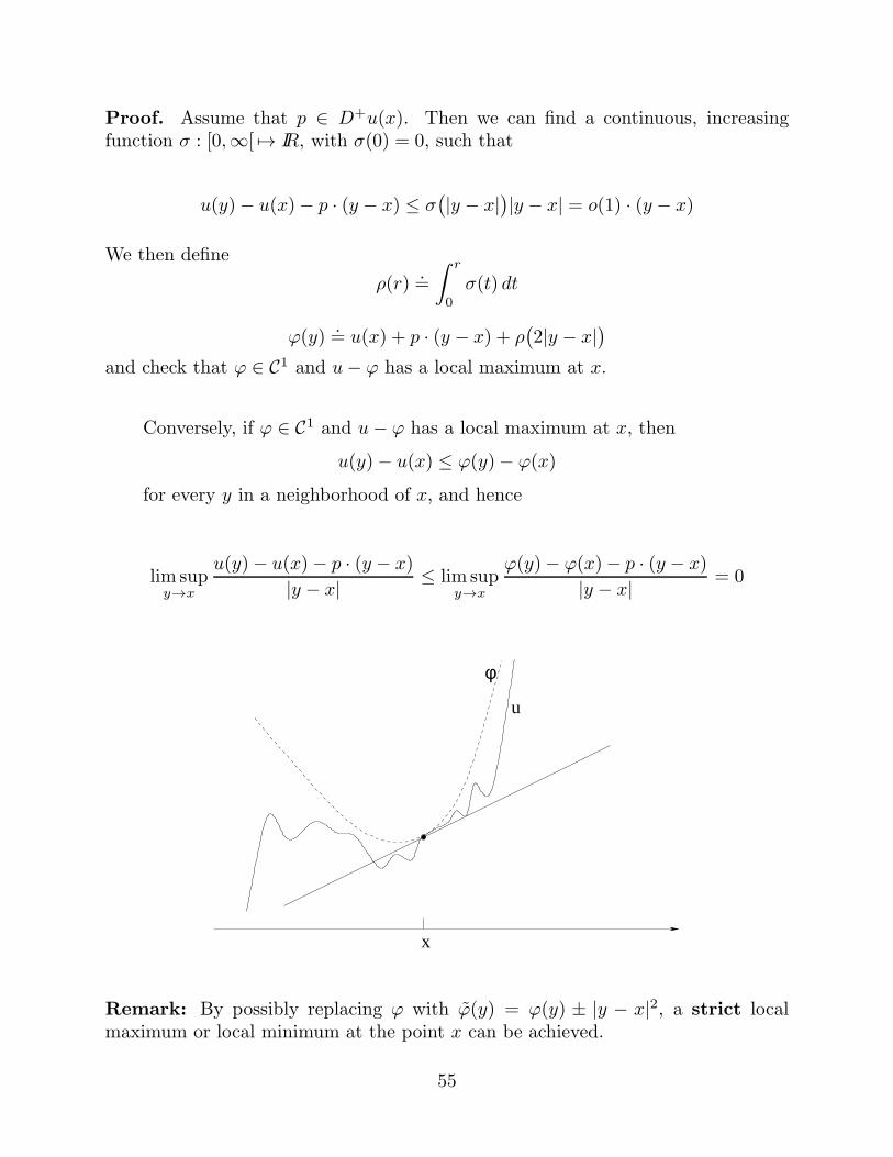
Proof. Assume that p ∈ D+u(x). Then we can find a continuous, increasingfunction σ : [0,∞[ 7→ IR, with σ(0) = 0, such that
u(y)− u(x)− p · (y − x) ≤ σ(|y − x|
)|y − x| = o(1) · (y − x)
We then define
ρ(r).=
∫ r
0
σ(t) dt
ϕ(y).= u(x) + p · (y − x) + ρ
(2|y − x|
)
and check that ϕ ∈ C1 and u− ϕ has a local maximum at x.
Conversely, if ϕ ∈ C1 and u− ϕ has a local maximum at x, then
u(y)− u(x) ≤ ϕ(y)− ϕ(x)
for every y in a neighborhood of x, and hence
lim supy→x
u(y)− u(x)− p · (y − x)
|y − x| ≤ lim supy→x
ϕ(y)− ϕ(x)− p · (y − x)
|y − x| = 0
x
φ
u
Remark: By possibly replacing ϕ with ϕ(y) = ϕ(y) ± |y − x|2, a strict localmaximum or local minimum at the point x can be achieved.
55

Properties of super- and sub-differentials
Lemma 2. Let u ∈ C(Ω). Then
(i) If u is differentiable at x, then
D+u(x) = D−u(x) =∇u(x)
(ii) If the sets D+u(x) and D−u(x) are both non-empty, then u is differentiable atx.
(iii) The sets of points where a one-sided differential exists:
Ω+ .=x ∈ Ω; D+u(x) 6= ∅
, Ω− .
=x ∈ Ω; D−u(x) 6= ∅
are both non-empty. Indeed, they are dense in Ω.
Proof of (i). Assume u is differentiable at x.
Trivially, ∇u(x) ∈ D±u(x).
On the other hand, if ϕ ∈ C1(Ω) is such that u−ϕ has a local maximum at x, then∇ϕ(x) = ∇u(x).
Hence D+u(x) cannot contain any vector other than ∇u(x).
56

y
1
2
x
ϕ
ϕ
u
u
ϕ
x0
Proof of (ii). Assume that the sets D+u(x) and D−u(x) are both non-empty.Then we can find ϕ1, ϕ2 ∈ C1(Ω) such that, for y near x,
ϕ1(x) = u(x) = ϕ2(x), ϕ1(y) ≤ u(y) ≤ ϕ2(y)
By comparison, this implies that u is differentiable at x and ∇u(x) = ∇ϕ1(x) =∇ϕ2(x).
Proof of (iii). Fix any ball B(x0, ρ) ⊂ Ω.
By choosing ε > 0 sufficiently small, the smooth function
ϕ(x).= u(x0)−
|x− x0|22ε
is strictly negative on the boundary of the ball, where |x− x0| = ρ.
Since u(x0) = ϕ(x0), the function u − ϕ attains a local minimum at an interiorpoint x ∈ B(x0, ρ).
By Lemma 1, the sub-differential of u at x is non-empty: ∇ϕ(x) = (x − x0)/ε ∈D−u(x).
57

Viscosity Solutions
F(x, u(x), ∇u(x)
)= 0 (HJ)
Definition 1. Let F : Ω× IR× IRn 7→ IR be continuous.
u ∈ C(Ω) is a viscosity subsolution of (HJ) if
F(x, u(x), p) ≤ 0 for every x ∈ Ω, p ∈ D+u(x).
u ∈ C(Ω) is a viscosity supersolution of (HJ) if
F(x, u(x), p) ≥ 0 for every x ∈ Ω, p ∈ D−u(x).
We say that u is a viscosity solution of (HJ) if it is both a supersolution anda subsolution in the viscosity sense.
Evolution equation: ut +H(t, x, u,∇u) = 0. (E)
Definition 2. u ∈ C(Ω) is a viscosity subsolution of (E) if, for every C1 functionϕ = ϕ(t, x) such that u− ϕ has a local maximum at (t, x), there holds
ϕt(t, x) +H(t, x, u,∇ϕ) ≤ 0.
u ∈ C(Ω) is a viscosity supersolution of (E) if, for every C1 function ϕ =ϕ(t, x) such that u− ϕ has a local minimum at (t, x), there holds
ϕt(t, x) +H(t, x, u,∇ϕ) ≥ 0.
58

• The definition of subsolution imposes conditions on u only on the set Ω+ of pointsx where the super-differential D+u(x) is non-empty. Even if u is merely continuous,say nowhere differentiable, this set is non-empty and dense in Ω.
• If u is a C1 function that satisfies
F(x, u(x), ∇u(x)
)= 0 (HJ)
at every x ∈ Ω, then u is also a solution in the viscosity sense.
• Viceversa, if u is a viscosity solution, then the equality (HJ) must hold at everypoint x where u is differentiable.If u is Lipschitz continuous, then by Rademacher’s theorem it is a.e. differentiable.Hence (HJ) holds a.e. in Ω.
Example 2. The function u(x) = |x| is a viscosity solution of
F (x, u, ux).= 1− |ux| = 0 (1)
defined on the whole real line. Indeed, u is differentiable and satisfies the equationat all points x 6= 0. Moreover, we have
D+u(0) = ∅, D−u(0) = [−1, 1].
To show that u is a subsolution, there is nothing else to check. To show that u is asupersolution, take any p ∈ [−1, 1]. Then 1− |p| ≥ 0, as required.
Notice that u(x) = |x| is NOT a viscosity solution of the equation
|ux| − 1 = 0 (2)
Indeed, at x = 0, taking p = 0 ∈ D−u(0) we find |0| − 1 < 0. Therefore, u(x) = |x|is a viscosity subsolution of (2), but not a supersolution.
59
Vanishing Viscosity Limits
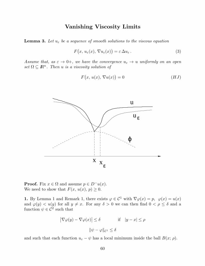
Lemma 3. Let uε be a sequence of smooth solutions to the viscous equation
F(x, uε(x), ∇uε(x)
)= ε∆uε . (3)
Assume that, as ε → 0+, we have the convergence uε → u uniformly on an openset Ω ⊆ IRn. Then u is a viscosity solution of
F(x, u(x), ∇u(x)
)= 0 (HJ)
u
uε
xεx
ϕ
Proof. Fix x ∈ Ω and assume p ∈ D−u(x).We need to show that F (x, u(x), p) ≥ 0.
1. By Lemma 1 and Remark 1, there exists ϕ ∈ C1 with ∇ϕ(x) = p, ϕ(x) = u(x)and ϕ(y) < u(y) for all y 6= x. For any δ > 0 we can then find 0 < ρ ≤ δ and afunction ψ ∈ C2 such that
∣∣∇ϕ(y)−∇ϕ(x)∣∣ ≤ δ if |y − x| ≤ ρ
‖ψ − ϕ‖C1 ≤ δ
and such that each function uε − ψ has a local minimum inside the ball B(x; ρ).
60

2. Let uε − ψ have a local minimum at xε ∈ B(x, ρ). Then
∇ψ(xε) = ∇u(xε), ∆u(xε) ≥ ∆ψ(xε).
F(x, uε(xε), ∇ψ(xε)
)≥ ε∆ψ(xε) (4)
3. Extract a convergent subsequence xε → x ∈ B(x, ρ).
Letting ε→ 0+ in (4) we have
F(x, u(x), ∇ψ(x)
)≥ 0. (5)
Choosing δ > 0 small we can make
∣∣u(x)− u(x)∣∣ ∣∣∇ψ(x)− p
∣∣
as small as we like.
By continuity, (5) yields F (x, u(x), p) ≥ 0.
Hence u is a supersolution. The other half of the proof is similar.
61

Comparison Theorems
Theorem 1. Let Ω ⊂ IRn be a bounded open set. Assume that u1, u2 ∈ C(Ω) are,respectively, viscosity sub- and supersolutions of
u+H(x,Du) = 0 x ∈ Ω, (HJ)
andu1 ≤ u2 on ∂Ω. (6)
Moreover, assume that the function H : Ω× IRn 7→ IR satisfies∣∣H(x, p)−H(y, p)
∣∣ ≤ ω(|x− y|
(1 + |p|
)), (7)
where ω : [0,∞[ 7→ [0,∞[ is continuous and non-decreasing, with ω(0) = 0. Then
u1 ≤ u2 on Ω. (8)
Proof. Easy case: u1, u2 smooth.
If (8) fails, then u1 − u2 attains a positive maximum at x0 ∈ Ω.Therefore p
.= ∇u1(x0) = ∇u2(x0).
By definition of sub- and supersolution:
u1(x0) +H(x0, p) ≤ 0,
u2(x0) +H(x0, p) ≥ 0.(9)
Hence u1(x0)− u2(x0) ≤ 0 reaching a contradiction.
Ω Ω
u2
u1
x0
x0
u2
1u
62

In the non-smooth case, we can reach again a contradiction provided that wecan find a point x0 such that
(i) u1(x0) > u2(x0),
(ii) some vector p lies at the same time in the upper differential D+u1(x0) and inthe lower differential D−u2(x0).
A natural candidate for x0 is a point where u1−u2 attains a global maximum.However, one of the sets D+u1(x0) or D
−u2(x0) may be empty!
To proceed further, the key observation is that we don’t need to compare valuesof u1 and u2 at exactly the same point. Indeed, to reach a contradiction, it sufficesto find nearby points xε and yε such that
(i’) u1(xε) > u2(yε),
(ii’) some vector p lies at the same time in the upper differential D+u1(xε) and inthe lower differential D−u2(yε).
yε xε
Ω
u2
u1
63
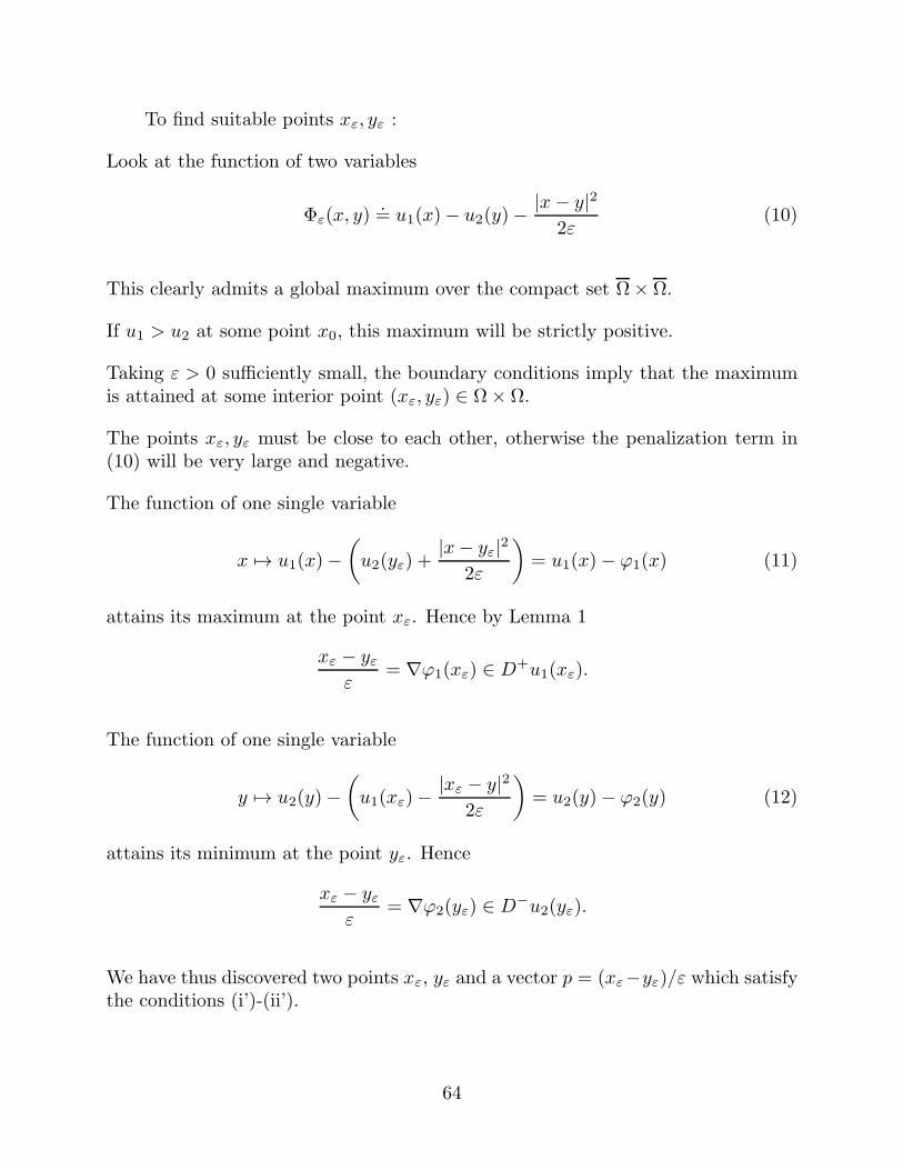
To find suitable points xε, yε :
Look at the function of two variables
Φε(x, y).= u1(x)− u2(y)−
|x− y|22ε
(10)
This clearly admits a global maximum over the compact set Ω× Ω.
If u1 > u2 at some point x0, this maximum will be strictly positive.
Taking ε > 0 sufficiently small, the boundary conditions imply that the maximumis attained at some interior point (xε, yε) ∈ Ω× Ω.
The points xε, yε must be close to each other, otherwise the penalization term in(10) will be very large and negative.
The function of one single variable
x 7→ u1(x)−(u2(yε) +
|x− yε|22ε
)= u1(x)− ϕ1(x) (11)
attains its maximum at the point xε. Hence by Lemma 1
xε − yεε
= ∇ϕ1(xε) ∈ D+u1(xε).
The function of one single variable
y 7→ u2(y)−(u1(xε)−
|xε − y|22ε
)= u2(y)− ϕ2(y) (12)
attains its minimum at the point yε. Hence
xε − yεε
= ∇ϕ2(yε) ∈ D−u2(yε).
We have thus discovered two points xε, yε and a vector p = (xε−yε)/ε which satisfythe conditions (i’)-(ii’).
64
Proof of Theorem 1.
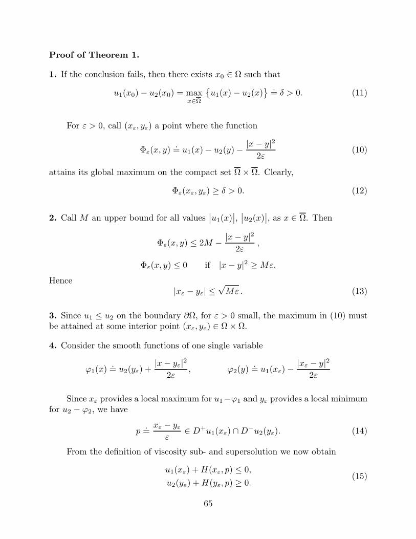
1. If the conclusion fails, then there exists x0 ∈ Ω such that
u1(x0)− u2(x0) = maxx∈Ω
u1(x)− u2(x)
.= δ > 0. (11)
For ε > 0, call (xε, yε) a point where the function
Φε(x, y).= u1(x)− u2(y)−
|x− y|22ε
(10)
attains its global maximum on the compact set Ω× Ω. Clearly,
Φε(xε, yε) ≥ δ > 0. (12)
2. Call M an upper bound for all values∣∣u1(x)
∣∣,∣∣u2(x)
∣∣, as x ∈ Ω. Then
Φε(x, y) ≤ 2M − |x− y|22ε
,
Φε(x, y) ≤ 0 if |x− y|2 ≥Mε.
Hence|xε − yε| ≤
√Mε . (13)
3. Since u1 ≤ u2 on the boundary ∂Ω, for ε > 0 small, the maximum in (10) mustbe attained at some interior point (xε, yε) ∈ Ω× Ω.
4. Consider the smooth functions of one single variable
ϕ1(x).= u2(yε) +
|x− yε|22ε
, ϕ2(y).= u1(xε)−
|xε − y|22ε
Since xε provides a local maximum for u1−ϕ1 and yε provides a local minimumfor u2 − ϕ2, we have
p.=xε − yε
ε∈ D+u1(xε) ∩D−u2(yε). (14)
From the definition of viscosity sub- and supersolution we now obtain
u1(xε) +H(xε, p) ≤ 0,
u2(yε) +H(yε, p) ≥ 0.(15)
65

5. Observing that
δ ≤ Φε(xε, yε) ≤ u1(xε)− u2(xε) +∣∣u2(xε)− u2(yε)
∣∣− |xε − yε|22ε
,
we see that∣∣u2(xε)− u2(yε)
∣∣− |xε − yε|22ε
≥ 0
and hence, by the uniform continuity of u2,
|xε − yε|22ε
→ 0 as ε→ 0. (16)
6. Subtracting the second from the first inequality in (15) we obtain
δ ≤ Φε(xε, yε)
≤ u1(xε)− u2(yε)
≤∣∣H(xε, p)−H(yε, p)
∣∣
≤ ω((|xε − yε| ·
(1 + |xε − yε|ε−1
)).
(17)
This yields a contradiction, Indeed, by (13) and (16) the right hand side of (17) canbe made arbitrarily small by letting ε→ 0.
Corollary 1. Let Ω ⊂ IRn be a bounded open set. Let the Hamiltonian function Hsatisfy the equicontinuity assumption (7). Then the boundary value problem
u+H(x,Du) = 0 x ∈ Ω
u = ψ x ∈ ∂Ω
admits at most one viscosity solution.
66

Uniqueness for the Cauchy Problem
ut +H(t, x,Du) = 0 (t, x) ∈ ]0, T [×IRn, (18)
u(0, x) = g(x) x ∈ IRn. (19)
(H1) H is uniformly continuous on [0, T ]×IRn×K, for every compact set K ⊂ IRn.
(H2) There exists a continuous, non-decreasing function ω : [0,∞[×[0,∞[ withω(0) = 0 such that
∣∣H(t, x, p)−H(t, y, p)∣∣ ≤ ω
(|x− y|
(1 + |p|
)).
Theorem 2. Let the function H : [0, T ] × IRn × IRn satisfy the equicontinuityassumptions (H1)-(H2). Let u1, u2 be uniformly continuous sub- and super-solutionsof (18) respectively. If u1(0, x) ≤ u2(0, x) for all x ∈ IRn, then
u1(t, x) ≤ u2(t, x) for all (t, x) ∈ [0, T ]× IRn.
Corollary 2. Let the function H satisfy the assumptions (H1)-(H2). Then theCauchy problem
ut +H(t, x,Du) = 0 (t, x) ∈ ]0, T [×IRn
u(0, x) = g(x) x ∈ IRn
admits at most one uniformly continuous viscosity solution u : [0, T ]× IRn 7→ IR.
67

Sketch of the proof of Theorem 2.
Assume, on the contrary, that u1 > u2 at some point (t, x).Then for some λ > 0 we still have
u1(t, x)− λt > u2(t, x)
Assume that we can find a global maximum:
u1(t0, x0)− λt0 − u2(t0, x0) = supt∈[0,T ], x∈IRn
u1(t, x)− λt− u2(t, x)
Clearly, t0 > 0. If u1, u2 are smooth, then
∇u1(t0, x0) = ∇u2(t0, x0), ∂t u1(t0, x0)− λ ≥ ∂t u2(t0, x0) (20)
On the other hand, by assumptions we have
∂t u1(t0, x0) +H(t0, x0, u1,∇u1) ≤ 0
∂t u2(t0, x0) +H(t0, x0, u1,∇u1) ≥ 0(21)
Together (20) and (21) yield a contradiction.
Toward the general case - two technical difficulties:
1. The supremum of u1 − u2 − λt may only be approached as |x| → ∞.
2. The functions u1, u2 may not admit upper or lower differentials at the pointwhere the maximum is attained.
Key idea: look at the function of double variables
Φε(t, x, s, y).= u1(t, x)− u2(s, y)− λ(t+ s)− ε
(|x|2 + |y|2
)− 1
ε
(|x− y|2 + |t− s|2
)
The first penalization term guarantees that a global maximum is attained.
The second penalization term guarantees that, at the point (tε, xε, sε, yε) wherethe maximum is attained, one has tε ≈ sε and xε ≈ yε.
68

Extensions
• Discontinuous solutions
• Second order equations
u : Ω 7→ IR is upper semicontinuous at x0 if
lim supx→x0
u(x) ≤ u(x0),
u : Ω 7→ IR is lower semicontinuous at x0 if
lim infx→x0
u(x) ≥ u(x0),
u
0x x0
u
A nonlinear operator F = F (x, u, Du, D2u) is (possibly degenerate) elliptic if
F (x, u, p,X) ≤ F (x, u, p, X + Y ) whenever Y ≥ 0
(i.e. whenever the symmetric matrix Y is non-negative definite)
69

General nonlinear elliptic equation:
F (x, u, Du, D2u) = 0 (22)
An upper semicontinuous function u : Ω 7→ IR is a viscosity subsolution ofthe degenerate elliptic equation (22) if, for every ϕ ∈ C2(Ω), at each point x0 whereu− ϕ has a local maximum there holds
F(x0, u(x0), Dϕ(x0), D
2ϕ(x0))≤ 0.
A lower semicontinuous function u : Ω 7→ IR is a viscosity supersolution ofthe degenerate elliptic equation (22) if, for every ϕ ∈ C2(Ω), at each point x0 whereu− ϕ has a local minimum there holds
F(x0, u(x0), Dϕ(x0), D
2ϕ(x0))≥ 0.
Comparison and uniqueness results:
R. Jensen, Arch. Rat. Mech. Anal. (1988)
H. Ishii, Comm. Pure Appl. Math. (1989)
70

Systems of Hamilton-Jacobi Equations
wt +H(x, Dw) = 0 w : Ω 7→ IRn
1. Systems of conservation laws in one space dimension
ut + f(u)x = 0 (23)
u = (u1, . . . , un) conserved quantities
f = (f1, . . . , fn) : IRn 7→ IRn fluxes
Since (23) is in divergence form, we can take w such that
wx = u wt = f(u)
This yields the H-J system of equations
wt + f(wx) = 0
71

2. Non-cooperative m-persons differential games
x =
m∑
i=1
fi(x, ui). (23)
t 7→ ui(t) ∈ Ui is the control chosen by the i-th player, whose aim is to minimizehis cost functional
Ji.=
∫ T
t
hi(x(s), ui(s)
)ds+ gi
(x(T )
). (24)
Let Vi(t, x) be the expected cost for the i-th player (if he behaves optimally), if thesystem starts at state x at time t.
If such value function V = (V1, . . . , Vm) exists, it should provide a solution to thesystem of Hamilton-Jacobi equations
∂t Vi +Hi(x,∇V1, · · · ,∇Vm) = 0, (25)
with terminal dataVi(T, x) = gi(x). (26)
The Hamiltonian functions Hi are defined as follows.Assume that, for every given x ∈ IRn and pj = ∇Vj ∈ IRn, there exist an optimalchoice u∗j (x, pj) ∈ Uj for the j-th player, such that
fj(x, u∗j (x, pj)
)· pj + hj
(x, u∗j (x, pj)
)= min
ω
fj(x, ω) · pj + hj(x, ω)
Then the Hamiltonian functions in (25) are
Hi(x, p1, . . . , pm).=
m∑
j=1
fj(x, u∗j (x, pj)
)· pi + hi
(x, u∗i (x, pi)
)
(No general existence, uniqueness theory is yet available for these systems)
72

Sufficient Conditions for Optimality
x = f(x, u) t ∈ [0, T ], x(0) = x0 (1)
Family of admissible control functions: U .=u : [0, T ] 7→ U
For u(·) ∈ U , the trajectory of (1) is t 7→ x(t, u)
Terminal constraint
x(T ) ∈ S (2)
Mayer problem, free terminal point:
maxu∈U
ψ(x(T, u)
)(3)
Sufficient Condition: Existence + PMP.
Assume that the optimization problem (1)–(3) admits an optimal solution.Let u1, u2, . . . , uN be the set of all control functions that staisfy the PontryaginMaximum Principle. If
ψ(x(T, uk)
)= min
1≤j≤Nψ(x(T, uj)
)
Then the control uk is optimal.
73

Example 1.
(x1, x2) = (u, x21) u ∈ [−1, 1], (x1, x2)(0) = (0, 0)
maxu∈U
x2(T ) with constraint x1(T ) = 0
2
0 1 2− 1
x
x1
If t 7→ x∗(t) = x(t, u∗) is an optimal trajectory, the PMP yields
(p1, p2) = (−2x1p2, 0), p2(T ) ≥ 0
p1u∗ + p2x
21 = max
ω∈[−1,1]p1ω + p2x
21 =⇒ u∗ = sign p1
p2(t) ≡ p2 ≥ 0
p2 ≡ 0 =⇒ p1 ≡ p1 u∗(t) ≡ 0, x∗(t) ≡ (0, 0)
74

p2 ≡ 1 =⇒ p1 = −2x1
p1 = −2 sign p1, p1(0) = 0
x1 = sign p1 x2 = x21
Countably many controls uj satisfy the PMP.
Optimal controls:
u∗(t) =
1 if 0 < t < T/2−1 if T/2 < t < T
u∗(t) =
−1 if 0 < t < T/21 if T/2 < t < T
1
0 T
..
..
p =−2
p =2
T/j
p
x
x
1
1
2 x*
1
75

The Value Function
x(t) = f(x(t), α(t)
)s < t < T, (4)
x(s) = y. (5)
Here x ∈ IRn, while the control function α : [s, T ] 7→ A is required to take valuesinside a compact set A ⊂ IRm.
Optimization Problem: select a control T 7→ α∗(t) which minimizes the cost
J(s, y, α).=
∫ T
s
h(x(t), α(t)
)dt+ g
(x(T )
). (6)
Assumption: The functions f, g, h are Lipschitz continuous and uniformly bounded.
Dynamic Programming Approach: study the value function
u(s, y).= inf
α(·)J(s, y, α). (7)
76
Bellman’s Dynamic Programming Principle
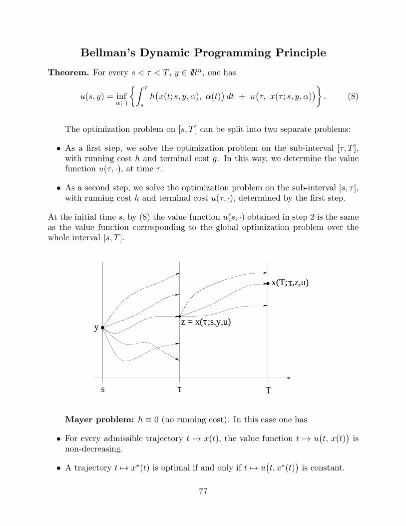
Theorem. For every s < τ < T , y ∈ IRn, one has
u(s, y) = infα(·)
∫ τ
s
h(x(t; s, y, α), α(t)
)dt + u
(τ, x(τ ; s, y, α)
). (8)
The optimization problem on [s, T ] can be split into two separate problems:
• As a first step, we solve the optimization problem on the sub-interval [τ, T ],with running cost h and terminal cost g. In this way, we determine the valuefunction u(τ, ·), at time τ .
• As a second step, we solve the optimization problem on the sub-interval [s, τ ],with running cost h and terminal cost u(τ, ·), determined by the first step.
At the initial time s, by (8) the value function u(s, ·) obtained in step 2 is the sameas the value function corresponding to the global optimization problem over thewhole interval [s, T ].
z = x( ;s,y,u)
x(T; ,z,u)
τs T
y τ
τ
Mayer problem: h ≡ 0 (no running cost). In this case one has
• For every admissible trajectory t 7→ x(t), the value function t 7→ u(t, x(t)
)is
non-decreasing.
• A trajectory t 7→ x∗(t) is optimal if and only if t 7→ u(t, x∗(t)
)is constant.
77

Proof. Call Jτ the right hand side of (8).
1. To prove that Jτ ≤ u(s, y), fix ε > 0 and choose a control α : [s, T ] 7→ A suchthat
J(s, y, α) ≤ u(s, y) + ε.
Observing that
u(τ, x(τ ; s, y, α)
)≤∫ T
τ
h(t, x(t; s, y, α)
)dt+ g
(x(T ; s, y, α)
),
we conclude
Jτ ≤∫ τ
s
h(t, x(t; s, y, α)
)dt+ u
(τ, x(τ ; s, y, α)
)
≤ J(s, y, α)
≤ u(s, y) + ε.
Since ε > 0 is arbitrary, this first inequality is proved.
2. To prove that u(s, y) ≤ Jτ , fix ε > 0. Then there exists a control α′ : [s, τ ] 7→ Asuch that ∫ τ
s
h(t, x(t; s, y, α′)
)dt+ u
(τ, x(τ ; s, y, α′)
)≤ Jτ + ε
Moreover, there exists a control α′′ : [τ, T ] 7→ A such that
J(τ, x(τ ; s, y, α′), α′′) ≤ u
(τ, x(τ ; s, y, α′)
)+ ε.
One can now define a new control α : [s, T ] 7→ A as the concatenation of α′, α′′:
α(t).=
α′(t) if t ∈ [s, τ ],α′′(t) if t ∈ ]τ, T ].
This yieldsu(s, y) ≤ J(s, y, α) ≤ Jτ + 2ε.
with ε > 0 arbitrarily small.
78

The Hamilton-Jacobi-Bellman Equation
x(t) = f(x(t), α(t)
)s < t < T, (4)
x(s) = y, α : [s, T ] 7→ A (5)
J(s, y, α).=
∫ T
s
h(x(t), α(t)
)dt+ g
(x(T )
). (6)
u(s, y).= inf
α(·)J(s, y, α). (7)
Lemma (Regularity of the Value Function). Let f, g, h, be uniformly boundedand Lipschitz continuous. Then the value function u is uniformly bounded andLipschitz continuous on [0, T ]× IRn.
Theorem (Characterization of the Value Function). The value functionu = u(s, y) is the unique viscosity solution of the Hamilton-Jacobi-Bellman equation
−[ut +H(x,∇u)
]= 0 (t, x) ∈ ]0, T [×IRn, (9)
with terminal condition
u(T, x) = g(x) x ∈ IRn, (10)
and Hamiltonian function
H(x, p).= min
a∈A
f(x, a) · p+ h(x, a)
. (11)
79

Proof. To show that u is a viscosity subsolution of
−[ut +min
a∈A
f(x, a) · ∇u+ h(x, a)
]= 0 (9)
let ϕ ∈ C1(]0, T [×IRn
). We need to show:
(P1) If u− ϕ attains a local maximum at a point (t0, x0) ∈]0, T [×IRn, then
ϕt(t0, x0) + mina∈A
f(x0, a) · ∇ϕ(t0, x0) + h(x0, a)
≥ 0. (12)
We can assume that
u(t0, x0) = ϕ(t0, x0), u(t, x) ≤ ϕ(t, x) for all t, x.
If (12) does not hold, then there exists a ∈ A and θ > 0 such that
ϕt(t0, x0) + f(x0, a) · Dϕ(t0, x0) + h(x0, a) < −θ. (13)
We shall derive a contradiction by showing that this control value a is “too good tobe true”. Namely, by choosing a control function α(·) with α(t) ≡ a for t ∈ [t0, t0+δ]and such that α is nearly optimal on the remaining interval [t0 + δ, T ], we obtaina total cost J(t0, x0, α) strictly smaller than u(t0, x0).
f(x ,a)0
t
u
ϕ
80

By continuity,
ϕt(t0, x0) + f(x0, a) · Dϕ(t0, x0) + h(x0, a) < −θ (13)
impliesϕt(t, x) + f(x, a) · Dϕ(t, x) < −h(x, a)− θ (14)
whenever t ≈ t0 and x ≈ x0. Let x(t).= x(t; t0, x0, a) be the solution of
x(t) = f(x(t), a
)x(t0) = x0.
Then
u(t0 + δ, x(t0 + δ)
)− u(t0, x0) ≤ ϕ
(t0 + δ, x(t0 + δ)
)− ϕ(t0, x0)
=
∫ t0+δ
t0
d
dtϕ(t, x(t)
)dt
=
∫ t0+δ
t0
ϕt
(t, x(t)
)+ f
(x(t), a
)· Dϕ
(t, x(t)
)dt
≤ −∫ t0+δ
t0
h(x(t), a
)dt− δθ
(15)
On the other hand, the Dynamic Programming Principle
u(t0, x0) = infα(·)
∫ t0+δ
t0
h(x(t; t0, x0, α), α(t)
)dt + u
(t0 + δ, x(t0 + δ; t0, x0, α)
)
yields
u(t0 + δ, x(t0 + δ)
)− u(t0, x0) ≥ −
∫ t0+δ
t0
h(x(t), a
)dt. (16)
Together, (15) and (16) yield a contradiction, hence (P1) must hold.
81

To show that u is a viscosity supersolution of
−[ut +min
a∈A
f(x, a) · ∇u+ h(x, a)
]= 0 (9)
let ϕ ∈ C1(]0, T [×IRn
). We need to show:
(P2) If u− ϕ attains a local minimum at a point (t0, x0) ∈]0, T [×IRn, then
ϕt(t0, x0) + mina∈A
f(x0, a) · ∇ϕ(t0, x0) + h(x0, a)
≤ 0. (17)
We can assume that
u(t0, x0) = ϕ(t0, x0), u(t, x) ≥ ϕ(t, x) for all t, x. (18)
If (P2) fails, then there exists θ > 0 such that
ϕt(t0, x0) + f(x0, a) · Dϕ(t0, x0) + h(x0, a) > θ for all a ∈ A. (19)
In this case, we shall reach a contradiction by showing that no control function α(·)is good enough. Namely, whatever control function α(·) we choose on the initialinterval [t0, t0 + δ], even if during the remaining time [t0 + δ, T ] our control isoptimal, the total cost will still be considerably larger than u(t0, x0).
ϕ
u
t
f(x ,a)0
82

By continuity,
ϕt(t0, x0) + f(x0, a) · Dϕ(t0, x0) + h(x0, a) > θ for all a ∈ A (17)
impliesϕt(t, x) + f(x, a) · Dϕ(t, x) > θ − h(x, a) for all a ∈ A (20)
for all t ≈ t0 and x ≈ x0. Choose an arbitrary control function α : [t0, t0 + δ] 7→ A,and call t 7→ x(t) = x(t; t0, x0, α) the corresponding trajectory. We now have
u(t0 + δ, x(t0 + δ)
)− u(t0, x0) ≥ ϕ
(t0 + δ, x(t0 + δ)
)− ϕ(t0, x0)
=
∫ t0+δ
t0
d
dtϕ(t, x(t)
)dt
=
∫ t0+δ
t0
ϕt
(t, x(t)
)+ f
(x(t), α(t)
)· Dϕ
(t, x(t)
)dt
≥∫ t0+δ
t0
θ − h(x(t), α(t)
)dt
(21)Therefore, for every control function α(·),
u(t0 + δ, x(t0 + δ)
)+
∫ t0+δ
t0
h(x(t), α(t)
)dt ≥ u(t0, x0) + δθ. (22)
Taking the infimum of the left hand side of (22) over all control functions α, we seethat this infimum is still ≥ u(t0, x0) + δθ.
On the other hand, the Dynamic Programming Principle states that
u(t0, x0) = infα(·)
∫ t0+δ
t0
h(x(t; t0, x0, α), α(t)
)dt + u
(t0 + δ, x(t0 + δ; t0, x0, α)
)
in contradiction with (22). This establishes (P2).
Therefore, u is a viscosity solution.
83

Sufficient Conditions for Optimality
1. For each initial condition (s, y), construct a “candidate” optimal control αs,y :[s, T ] 7→ A, satisfying the PMP.
2. Consider the corresponding cost
u(s, y).= J(s, y, αs,y) (23)
3. Check whether v satisfies the Hamilton-Jacobi-Bellman equation
−[ut +min
a∈A
f(x, a) · ∇u+ h(x, a)
]= 0 (t, x) ∈ ]0, T [×IRn, (9)
in the viscosity sense, with terminal condition
u(T, x) = g(x) x ∈ IRn (10)
In the positive case, by uniqueness, u coincides with the minimum value function.Hence all controls αs,y are optimal.
The optimal control is found in feedback form:
α∗(t, x) = argmina∈A
f(x, a) · ∇u+ h(x, a)
at every point (t, x) where u is differentiable.
84

Regular Synthesis
For the optimization problem (4)–(6), let u = u(t, x) be the minimum valuefunction, defined at (7).
Theorem. Let v : [0, T ]× IRn 7→ IR be a continuous function such that
v ≥ u (23)
v(T, x) = g(x) x ∈ IRn . (24)
Assume that there exist C1 manifolds M1, . . . ,MN ⊂ [0, T ]×IRn of dimension ≤ n,such that v is continuously differentiable and satisfies
vt +mina∈A
f(x, a) · ∇v + h(x, a)
= 0 (9)
on the open set ]0, T [×IRn \⋃Mj.
Then v = u on [0, T ]× IRn.
Remark. Here we only require (9) to be satisfied on an open set where v is C1.Nothing has to be checked at points (t, x) ∈ Mj .
On the other hand, we assume that v is sufficiently regular, i.e. v ∈ C1 outsidefinitely many manifolds.
In this case, we say that the optimization problem admits a regular synthesis.
Proof. We only need to show that u ≥ v.
1. Assume u(t0, x0) < v(t0, x0). By continuity,
u(t, x) + 3ε ≤ v(t, x) (24)
for some ε > 0 and all (t, x) in a neighborhood of (t0, x0).
85

2. Since u is the infimum of the cost, there exists a control α∗ : [t0, T ] 7→ A suchthat the trajectory t 7→ x∗(t) satisfies
x∗(t0) = x0, x∗(t) = f(x∗(t), α∗(t)
)for a.e. t ∈ [t0, T ]
∫ T
t0
h(x∗(t), α∗(t)
)dt+ g
(x∗(T )
)≤ u(t0, x0) + ε (25)
3. The set of piecewise constant controls is L1 dense on the set of all measurablecontrols α : [t0, T ] 7→ A. Hence we can find a piecewise constant control α♣ suchthat, calling t 7→ x♣(t) the solution to
x♣(t) = f(x♣(t), α♣(t)
), x♣(T ) = x∗(T ),
also α♣ is nearly optimal. Its cost is
J(α♣) =
∫ T
t0
h(x♣(t), α♣(t)
)dt+ g
(x♣(T )
)≤ u
(t0, x
♣(t0))+ 2ε (26)
We shall obtain a contradiction by showing that the total cost for α♣ is
J(α♣) ≥ v(t0, x
♣(t0))≥ u
(t0, x
♣(t0))+ 3ε
00 Tt
x#
x*
x
t t
x (T)=x (T)*#
21
86

4. Let t0 < t1 < · · · < tm = T be the times where u♣ has a jump.
If we show that, for every j = 1, . . . ,m
∫ tj
tj−1
h(x♣(t), u♣(t)
)dt ≥ v
(tj−1, x
♣(tj−1))− v(tj , x
♣(tj))
(27)
we reach a contradiction. Indeed, summing over j we obtain
∫ T
t0
h(x♣(t), u♣(t)
)dt ≥ v(t0, x
♣(t0))− v(T, x♣(T )
).
Then the total cost using the control α♣ is
∫ T
t0
h(x♣(t), u♣(t)
)dt+ g
(x∗(T )
)≥ v(t0, x
♣(t0)). (28)
5. It remains to prove (27). More generally we show that, for every constant controlα(t) ≡ a and every trajectory
x(t) = f(x(t), a
)t ∈ [τ, τ ′]
we have ∫ τ ′
τ
h(x(t), a
)dt ≥ v(τ, x(τ)
)− v(τ ′, x(τ ′)
)(29)
87

By a transversality argument, we can find a sequence of trajectories
xm = f(xm(t), a
)
uniformly converging to x, such that each xm crosses each manifold Mj only atfinitely many times. Since xm(t) /∈ ∪Mj outside these crossing times, the Hamilton-Jacobi-Bellman equation
vt +mina∈A
f(x, a) · ∇v + h(x, a)
= 0 (9)
yieldsd
dtv(t, xm(t)
)+ h(xm, a) = vt +∇v · f(xm, a) + h(xm, a) ≥ 0
Therefore, integrating over [τ, τ ′]
∫ τ ′
τ
h(xm(t), a
)dt+ v(τ ′, xm(τ ′)
)− v(τ, xm(τ)
)≥ 0
Letting m→ ∞ we conclude
∫ τ ′
τ
h(x(t), a
)dt ≥ v(τ, x(τ)
)− v(τ ′, x(τ ′)
). (29)
x
T0
x
M
M
M1
2
3
x
m
88
Nonlinear First Order P.D.E.
The Method of Characteristics
vt +H(x,∇v) = 0 (30)
v(τ, x) = v(x), (31)
Assume H, v smooth. Call p.= ∇v, so that p = (p1, . . . , pn) = (vx1
, . . . , vxn)
∂2v
∂xi∂xj=∂pi∂xj
=∂pj∂xi
.
Differentiating (30) w.r.t. xi one obtains
∂pi∂t
=∂2v
∂xi∂t= −∂H
∂xi−∑
j
∂H
∂pj
∂pi∂xj
The total derivative of pi along a curve t 7→ x(t) is
d
dtpi(t, x(t)
)=∂pi∂t
+∑
j
xj∂pi∂xj
= −∂H∂xi
+∑
j
(xj −
∂H
∂pj
)∂pi∂xj
(32)
By choosing x = ∂H/∂p, the last term in (32) disappears.
89

Method of characteristics:
For each x, solve the Hamiltonian system of O.D.E’s
xi =∂H
∂pi(x, p) ,
pi = −∂H∂xi
(x, p) ,
xi(τ) = xi ,
pi(τ) =∂v
∂xi(x) .
(33)
Write the solution as t 7→ x(t, x), t 7→ p(t, x).
Observing that ∇v(t, x(t, x)
)= p(t, x) and
d
dtv(t, x(t, x)
)= vt +∇v · x = −H(x, p) + p · ∂H
∂p
we obtain
v(t, x(t, x)
)= v(τ, x) +
∫ t
τ
(−H(x, p) + p · ∂H
∂p
)ds
x
τ
x(t, x)−
t
−
90

Pontryagin’s Maximum Principle and
the P.D.E. of Dynamic Programming
x = f(x, α) α(t) ∈ A (34)
Minimize a cost functional involving a running cost h and a terminal cost g:
Js,y(α).=
∫ T
s
h(x(t), α(t)
)dt + g
(x(T )
). (35)
Here t 7→ x(t) is the trajectory of (34) corresponding to the control α : [s, T ] 7→ Aand with initial data x(s) = y.
Value function: v(t, x).= inf
α(·)J t,x(α) (36)
is a viscosity solution of the Hamilton-Jacobi-Bellman equation
−[vt +H(x,∇v)
]= 0 (37)
withH(x, p)
.= min
a∈A
p · f(x, a) + h(x, a)
. (38)
On a region where v is smooth, the H-J equation (37) can be solved by the methodof characteristics. Assume
H(x, p) = p · f(x, a∗(x, p)
)+ h(x, a∗(x, p)
)= min
a∈A
p · f(x, a) + h(x, a)
. (38)
At the point α∗ where the minimum is attained, one has
p · ∂f∂a
(x, α∗) +∂h
∂a(x, α∗) = 0 .
Hence the Hamiltonian system (33) takes the form
x = f(x, α∗(x, p)
)
p = −p · ∂f∂x
(x, α∗(x, p)
)− ∂h
∂x
(x, α∗(x, p)
) (39)
The existence of an adjoint vector t 7→ p(t) satisfying the linear evolution equationin (39) and the minimality condition (38) is a well known necessary condition foroptimality, stated in the Pontryagin Maximum Principle.
91
References
• General theory of differential inclusions
[AC] J. P. Aubin and A. Cellina, Differential Inclusions, Springer, 1984.
[D] K. Deimling, Multivalued Differential Equations, De Gruyter, 1992.
• Control systems: basic theory and the Pontryagin Maximum Principle
[Ce] L. Cesari, Optimization - Theory and Applications, Springer, 1983.
[FR] W. H. Fleming and R. W. Rishel, Deterministic and Stochastic Optimal Con-trol, Springer, 1975.
[LM] E. B. Lee and L. Markus, Foundations of Optimal Control Theory, Wiley, 1967.
[PBGM] L. S. Pontryagin, V. Boltyanskii, R. V. Gamkrelidze and E. F. Mishenko, TheMathematical Theory of Optimal Processes, Wiley, 1962.
• Geometric properties of reachable sets, local controllability
[JS] V. Jurdjevic and H. J. Sussmann, Controllability of nonlinear systems, J. Diff.Equat. 12 (1972), 95-116.
[S] H. J. Sussmann, A general theorem on local controllability, SIAM J. ControlOptim. 25 (1987), 158-194.
[J] V. Jurdjevic, Geometric Control Theory, Cambridge University Press, 1997.
• Existence of optimal controls
[F] A. F. Filippov, On certain questions in the theory of optimal control, SIAM J.Control Optim. 1 (1962), 76-84.
• Nonlinear Bang-Bang Theorems
[N] L. W. Neustadt, The existence of optimal controls in absence of convexityconditions, J. Math. Anal. Appl. 7 (1963), 110-117.
92

[BP] A. Bressan and B. Piccoli, A Baire category approach to the bang-bang prop-erty, J. Diff. Equat. 116 (1995), 318-337.
• Extensions of the Pontryagin Maximum Principle
[C1] F. H. Clarke, The maximum principle with minimal hypotheses, SIAM J. Con-trol Optim. 14 (1976), 1078-1091.
[C2] F. H. Clarke, Optimization and Nonsmooth Analysis, Wiley-Interscience, 1983.
[K] A. J. Krener, The high order maximal principle and its applications to singularextremals, SIAM J. Control Optim. 15 (1977), 256-293.
• Viscosity solutions to Hamilton-Jacobi equations
[Ba] G. Barles, Solutions de viscosite des equations de Hamilton-Jacobi, Springer,1994.
[BC] M. Bardi and I. Capuzzo Dolcetta, Optimal Control and Viscosity Solutions ofHamilton-Jacobi-Bellman Equations, Birkhauser, 1997.
[CIL] M. G. Crandall, H. Ishii and P. L. Lions, User’s guide to viscosity solutions ofsecond order partial differential equation, Bull. Amer. Math. Soc. 27 (1992),1-67.
[TTN] D. V. Tran, M. Tsuji and D. T. S. Nguyen, The Characteristic Method andits Generalizations for First Order Nonlinear Partial Differential Equations,Chapman&Hall/CRC, 1999.
• Regular feedback synthesis, sufficient conditions for optimality
[FR] W. H. Fleming and R. W. Rishel, Deterministic and Stochastic Optimal Con-trol, Springer, 1975.
[PS] B. Piccoli and H. J. Sussmann, Regular synthesis and sufficiency conditions foroptimality, SIAM J. Control Optim. 39 (2000), 359-410.
93