an introductory view of the ocean

Chapter 2

An introductory view of the ocean

Many aspects of the ocean are challenging tounderstand, including how the ocean stores andredistributes heat over the globe, how life hascolonised the ocean and how carbon is cycledbetween the ocean, atmosphere and land. Toanswer these questions, we need to adopt a holis-tic view to understand the relevant physical,chemical and biological processes, and how theyare connected to each other. For example, a west-ern boundary current, like the Gulf Stream, has arange of signatures: a rapid transfer of heat, nutri-ents and carbon along the current, enhanced con-trasts in physical, chemical and biological proper-ties across the current, and increased exchanges ofheat, moisture and dissolved gases with the over-lying atmosphere.

A difficulty in understanding the ocean, ascompared to the atmosphere, is the problem oftaking observations due to the ocean being a moreinaccessible and hostile environment. To counterthat difficulty, a range of different techniqueshave been developed to unravel how the ocean cir-culates, drawing on a combination of ship-basedmeasurements, remote sensing from space andfreely drifting floats spreading throughout theocean.

In this chapter, we provide an introductoryview of the large-scale ocean circulation, and basicproperty distributions (Plates 2 to 7), as well asbriefly introduce the atmospheric circulation, andthen discuss how life flourishes in the ocean and,finally, how carbon is cycled in the ocean. Thismaterial provides a starting point for the rest ofthe book.

2.1 Ocean circulation

Water has a very low viscosity compared withmost other liquids and moves easily wheneverthere is forcing, rather than moving sluggishlylike it does in a soggy marsh. The ocean circulatesdue to a combination of mechanical and densityforcing:

� Air moving over the surface water provides africtional drag, depending on the difference inthe speed of both fluids. Since the atmospheremoves so much faster than the ocean, there isa transfer of momentum into the ocean, ulti-mately driving most of the currents in the upperocean.

� Variations in the gravitational accelerationacross the Earth from the Moon lead to bulgesof water forming around the Earth, orientatedtowards and away from the Moon. As the Earthrotates about its own axis, these bulges appearas a regular rise and fall of sea level at the coast,occurring typically once or twice a lunar day(24 hours 50 minutes). There are similar, albeitweaker, tidal oscillations formed by the gravita-tional forcing from the Sun. While tides are mostpronounced near the coast, they occur through-out the water column and can lead to enhancedmixing when the tidal flows interact with roughtopography.

� Surface density is altered through the exchangeof heat and fresh water with the atmosphere;increasing with surface cooling or evaporation.

17

18 PART I INTRODUCTION

deep ocean

mixed layer(end of winter)

thermocline

overturningcirculation

eddies

subtropicalgyre

windstress recirculations

boundarycurrents

subpolargyre

convection

y

x

z

Figure 2.1 A schematic view of thecirculation within an ocean basin,including recirculating gyres andoverturning. Surface winds induce thegyres containing western boundarycurrents, interior flows and eddies. Thehorizontal circulation is connected withsloping temperature and density surfaces(full line) in the interior. In the vertical,there is a surface mixed layer (dashedline) where convection occurs, togetherwith a thermocline, where there arestrong vertical temperature gradients,and deep waters with more uniformproperties.

In polar regions, density also increases throughcooling by any overlying ice or by the atmo-sphere over gaps in the ice, as well by the addi-tion of salt released when ice freezes. When-ever surface waters become denser than deeperwaters, convection occurs and the fluid verti-cally overturns. Density contrasts lead to hori-zontal pressure gradients, which then acceleratethe flow. Dense waters formed at high latitudescan sink to great depths and spread horizontallyover the ocean, replaced at the surface by lighterwaters, which then generate an overturningcirculation.

With the exception of the tidal oscillations, theocean moves relatively slowly, so that water takesmany days to cross a basin, leading to currentsbeing strongly constrained by the Earth’s rotation;this rotational constraint leads to ocean flows per-sisting, rather than being quickly dissipated (asinstead occurs for water sloshing from side to sidein a bath).

The pattern of ocean circulation is also affectedby topography, since deep flows move around anyphysical barriers and follow the pattern of chan-nels and gaps in the topography. Surface currentsare also sometimes influenced by the underlyingtopography, since currents often prefer to movearound a submerged bump, rather than movedirectly over the bump.

The combination of forcing, rotation andtopography leads to an intriguing range of phys-ical phenomena, as illustrated in Fig. 2.1: thereare strong boundary currents alongside some landboundaries, but not others; basin-scale circula-tions confined within continental barriers; over-turning circulations, including deep boundarycurrents; and vibrant, time-varying eddies occur-ring throughout the ocean.

Next we consider observational views of thesurface circulation and their connection to theunderlying temperature and density distribu-tions.

2.1.1 How does the surface flow vary?Beneath a thin surface boundary layer, ocean cur-rents follow the dynamic height of the sea surfacein the same manner that air moves along pres-sure contours, as depicted on a weather chart;the dynamic height is the displacement of anypressure surface from a reference surface, calledthe geoid. A glance at a global map of dynamicheight, as shown in Fig. 2.2, reveals several domi-nant, large-scale regimes:

� The ocean circulates on a horizontal scale ofseveral thousand kilometres between the con-tinents; these basin-scale circulations are calledgyres (Fig. 2.3a). These gyre circulations rotatein a clockwise manner in the subtropics of

2 AN INTRODUCTORY VIEW OF THE OCEAN 19

(a) dynamic height (cm)

−200 −40 40 120

0 5 10 25 50

(b) surface speed (cm s−1)

Figure 2.2 Different regimes for thenear-surface circulation (excluding africtional contribution from the wind)revealed in (a) mean dynamic height(contours with an interval of 10 cm andincreased to 20 cm over the SouthernOcean) and (b) surface speed (cm s−1)diagnosed from the gradient in meandynamic height (assuming geostrophicbalance with values excluded within 2◦ ofthe equator where this balance does notapply; see later Section 4.2.1). The dynamicheight is the displacement of a pressuresurface from a reference surface, called thegeoid. Below a thin surface boundary layer,the surface flow is directed approximatelyalong contours of dynamic height. Thereare large-scale recirculations within basins,referred to as gyres, including intensewestern, boundary currents, over much ofthe globe. In the Southern Ocean, thesurface flow is directed broadly eastwardand circumnavigates the globe, and isreferred to as the Antarctic CircumpolarCurrent. The dynamic height was takenfrom a combined dataset integratinginformation from surface drifters in theocean, remotely sensed measurements ofsea-surface height from altimetry, surfacewinds and measurements of the geoidfrom the GRACE gravity mission (Niileret al., 2003; Maximenko and Niiler, 2005).

the northern hemisphere and anticlockwise inthe subtropics of the southern hemisphere. Thegyre circulations rotate in the opposite sense athigher latitudes. This change in rotation of thegyres reflects the pattern of the overlying winds.The rotation of the flow is defined as cyclonicwhenever the rotation is in the same sense as therotation of the Earth, anticlockwise in the north-ern hemisphere and clockwise in the southernhemisphere.

� Accompanying these gyre circulations are vig-orous and narrow boundary currents along thewestern sides of the ocean basins, such as theGulf Stream in the North Atlantic, the BrazilCurrent in the South Atlantic, and the Kuroshioin the North Pacific (Fig. 2.2b).

� In the tropics, there is an equatorial current sys-tem consisting of reversing, zonal flows withhigh speeds. Over the tropics, currents are forcedby the prevailing westward winds: on either sideof the equator, there are two westward flow-ing equatorial currents, together with a narroweastward return flow in an equatorial countercurrent located between them; note that thespeed is not mapped within 2◦ of the equatorin Fig. 2.2b.

� Within the southern hemisphere, there aregaps between Antarctica and the northern landmasses, allowing an uninterrupted flow to cir-cumnavigate the globe roughly along latitudecircles (Fig. 2.3b). This eastward current, theAntarctic Circumpolar Current, extends from


eastwardsjet

(a) recirculations within ocean basins

tropics subtropicalgyre

subpolargyre

thermocline

deep ocean

mixed layer

thermocline

deep ocean

(b) zonal flow in Southern Ocean

mixed layer

plan view meridional section

plan view

meridional section

xy

xy

yz

yz

subtropicalgyre

subpolargyre

Figure 2.3 A schematic figure depicting (a) recirculating flows within ocean basins in the northern hemisphere and (b) near zonalflows within the Southern Ocean for a plan view (left panel) and a meridional section (right panel), including the base of the mixedlayer (dashed line). In (a), the circulations are associated with a thin thermocline in the tropics and a thicker thermocline in thesubtropical gyre, and a thin or seasonal thermocline over the subpolar gyre. In (b), an eastward wind-driven current in the SouthernOcean is associated with cold water outcropping on the poleward side of the current. On the equatorial side of the SouthernOcean, the near-zonal flows can interact with the gyre circulations in the Atlantic, Indian and Pacific basins.

the surface to the sea floor and is made up ofa series of narrow jets (regions of fast-movingflow). The Antarctic Circumpolar Current is anal-ogous to the fast moving Jet Stream in the upperatmosphere.

In addition to this network of persistent cur-rents covering the globe, there are also intensetime-varying circulations on smaller scales of sev-eral tens to a hundred kilometres, referred to asmesoscale eddies; although much smaller in size,these ocean eddies are analogous to atmosphericweather systems. Ocean eddies are preferentiallyformed along intense western boundary currents,such as the Gulf Stream, and within the jets mak-ing up the Antarctic Circumpolar Current.

2.1.2 How does the ocean vary inthe vertical?

The ocean has a characteristic vertical structure(Fig. 2.4a) consisting of a surface mixed layer,overlying a stratified upper ocean and a weaklystratified, deep ocean:

� The surface layer is well mixed with nearlyhomogeneous properties in the vertical. Thismixed layer varies in thickness from typically30 m to 500 m, as depicted in Fig. 2.4b–e. Thesurface layer is in direct contact with the atmo-sphere or, in polar regions, with overlying ice.The mixing in this layer is driven by turbulencegenerated by the wind blowing over the sea sur-face and by convection from the sinking of densewaters formed by surface cooling or evapora-tion to the atmosphere, or by brine release fromunderneath ice.

� In the upper ocean, there is usually a strongvertical temperature gradient, referred to asthe thermocline, which is typically accompa-nied by similar vertical gradients in salinityand density, such as seen extending from 500 mto 1500 m in Fig. 2.4. This strong stratifica-tion inhibits vertical mixing below the sur-face mixed layer. The thermocline can be sep-arated into an upper, seasonal thermoclineand a deeper, permanent or main thermocline.The seasonal thermocline strengthens from the


4 12 20

0

1

2

3

4

(b) potential temperature

θ

(°C)

dep

th (

km)

34 35 36 37

(c) salinity

26 27 28

(d) potential sigma

σθ

(kg m–3)150 200 250

(e) dissolved oxygen

(ml l–1)(g kg–1)

O2S

25

mixed layer

thermocline

deep ocean

(a) idealised profile

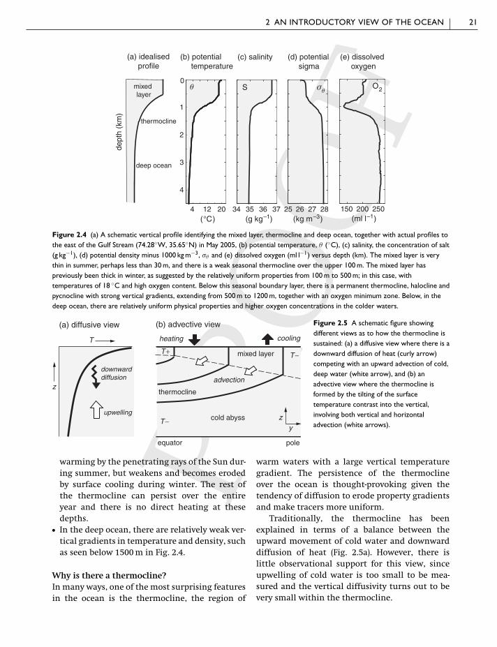
Figure 2.4 (a) A schematic vertical profile identifying the mixed layer, thermocline and deep ocean, together with actual profiles tothe east of the Gulf Stream (74.28◦W, 35.65◦N) in May 2005, (b) potential temperature, θ (◦C), (c) salinity, the concentration of salt(g kg−1), (d) potential density minus 1000 kg m−3, σθ and (e) dissolved oxygen (ml l−1) versus depth (km). The mixed layer is verythin in summer, perhaps less than 30 m, and there is a weak seasonal thermocline over the upper 100 m. The mixed layer haspreviously been thick in winter, as suggested by the relatively uniform properties from 100 m to 500 m; in this case, withtemperatures of 18 ◦C and high oxygen content. Below this seasonal boundary layer, there is a permanent thermocline, halocline andpycnocline with strong vertical gradients, extending from 500 m to 1200 m, together with an oxygen minimum zone. Below, in thedeep ocean, there are relatively uniform physical properties and higher oxygen concentrations in the colder waters.

(b) advective view

T+ T−

T−

thermocline

cold abyss

equator

advection

pole

heating cooling

(a) diffusive view

T

z

downwarddiffusion

upwelling

mixed layer

yz

Figure 2.5 A schematic figure showingdifferent views as to how the thermocline issustained: (a) a diffusive view where there is adownward diffusion of heat (curly arrow)competing with an upward advection of cold,deep water (white arrow), and (b) anadvective view where the thermocline isformed by the tilting of the surfacetemperature contrast into the vertical,involving both vertical and horizontaladvection (white arrows).

warming by the penetrating rays of the Sun dur-ing summer, but weakens and becomes erodedby surface cooling during winter. The rest ofthe thermocline can persist over the entireyear and there is no direct heating at thesedepths.

� In the deep ocean, there are relatively weak ver-tical gradients in temperature and density, suchas seen below 1500 m in Fig. 2.4.

Why is there a thermocline?In many ways, one of the most surprising featuresin the ocean is the thermocline, the region of

warm waters with a large vertical temperaturegradient. The persistence of the thermoclineover the ocean is thought-provoking given thetendency of diffusion to erode property gradientsand make tracers more uniform.

Traditionally, the thermocline has beenexplained in terms of a balance between theupward movement of cold water and downwarddiffusion of heat (Fig. 2.5a). However, there islittle observational support for this view, sinceupwelling of cold water is too small to be mea-sured and the vertical diffusivity turns out to bevery small within the thermocline.


60°S 30°S EQ 30°N 60°N

60°S 40°S 20°S EQ 20°N 40°N

5000

4000

3000

2000

1000

0

5000

4000

3000

2000

1000

0

2.5

50

10

θ Pacific

10

2.5

5

(a)

(b)

θ Atlantic

Figure 2.6 Observed meridionalsections, latitude versus depth (m), ofpotential temperature, θ (◦C), for (a) theAtlantic along 20◦W, and (b) the Pacificalong 170◦W; see Plates 2a and 3a forcolour and cruise track. There is generallya warm upper layer, referred to as thethermocline, overlying cold deep waters.The cold waters connect to the surfaceover the Southern Ocean. The sea floor isshaded in dark grey, revealing ridges andfracture zones. This section and manyothers are plotted from hydrographic datausing Ocean Data View developed byReiner Schlitzer.

Instead, the thermocline is a consequence ofthe three-dimensional circulation, effectively thesurface temperature gradient is tilted into the ver-tical by the vertical and horizontal flows (Fig. 2.5b).

Over the globe, the thermocline is shallow inthe tropics, deep at the mid latitudes, and even-tually disappears at high latitudes (Fig. 2.6). Thisthermocline variation reflects the pattern of theatmospheric forcing and the resulting horizon-tal circulation. At mid latitudes, a thickening ofthe thermocline is associated with the subtropicalgyres rotating anticyclonically (Fig. 2.3a), while athigh latitudes, a poleward thinning and eventualvanishing of the thermocline is associated withthe subpolar gyres rotating cyclonically and thestrong eastward flow in the Antarctic Circumpolar

Current (Fig. 2.3b); this dynamical connectionis discussed further in Sections 8.1.2, 8.4.1 and10.2.3.

2.1.3 How do water masses spread overthe globe?

Inferring the interior circulation is more challeng-ing than might be expected due to the difficultyof measuring the flow below the surface. Cluesas to the interior circulation are provided by thedistribution of water masses, defined in terms ofa collection of physical and biogeochemical prop-erties, including temperature, salinity, dissolvedoxygen and nutrient concentrations.

Water masses are formed in the surface mixedlayer where their properties are determined


NADW

salinity

AAIW

AABW

34.5

35

34.75

36

60°S 30°S EQ 30°N 60°N

60°S 40°S 20°S EQ 20°N 40°N

5000

4000

3000

2000

1000

0

5000

4000

3000

2000

1000

0

(a)

(b)

Atlantic

AAIW NPIW

NPDW

CDW

salinity

34

34.5

35

34.5

Pacific

Figure 2.7 Observed meridionalsections of salinity, S (g kg−1), theconcentration of salt in (a) the Atlanticalong 20◦W, and (b) the Pacific along170◦W; see Plates 2b and 3b. The saltdistribution is used to define the majorwater masses: AAIW, AntarcticIntermediate Water; AABW, AntarcticBottom Water; CDW, CircumpolarDeep Water; NADW, North AtlanticDeep Water; NPIW, North PacificIntermediate Water; and NPDW, NorthPacific Deep Water. These water massesare formed in discrete regions so thatthe water at any particular location isusually a composite of several watermasses.

through the exchange of heat, moisture and dis-solved gases with the atmosphere and, in polarregions, with ice, as well as biogeochemical prop-erties affected by biological activity (Fig. 2.4).

Once the water masses spread in the oceaninterior (Fig. 2.5b), they preferentially conservetheir salinity, as well as pressure-corrected vari-ants of temperature and density, referred toas potential temperature and potential density,respectively. There are striking contrasts in sur-face salinity between subtropical and subpolargyres, as well as between the Atlantic and Pacificbasins. Consequently, the interior salinity dis-tribution is very useful in revealing how watermasses spread. For example, salinity sectionsthrough the Atlantic and Pacific, as depicted inFig. 2.7, reveal the following pathways:

� Plumes of low salinity suggest a northwardspreading at mid depths and along the bottomfrom the Southern Ocean into the Atlantic andPacific basins, as well as a southward spread-ing in upper waters from high latitudes in thenorthern Pacific.

� Broader regions of higher salinity suggest asouthward spreading over several kilometresdepth in the Atlantic, as well as a more localisedsalty intrusion spreading at a depth of typically1 km, ultimately originating from the Mediter-ranean Sea.

Spreading of mode watersThe water-mass distribution can be viewed aslayers of water with nearly uniform properties,


(a) subtropical mode waters

(c) dense bottom waters

(b) fresh intermediate waters

Figure 2.8 Global distribution of modewaters: (a) subtropical mode watersformed on the western side (lightshading), eastern side (medium shading)and the poleward side (dark shading) ofthe gyre, including subpolar mode waterin the North Atlantic, North Pacificcentral mode water and Sub-Antarcticmode water in the southern hemisphere,together with cartoons of the gyrecirculation. (b) Fresh intermediate modewaters including Labrador Sea Water(dark shading, σθ = 27.8), North PacificIntermediate Water (light shading,σθ = 27.0) and Antarctic IntermediateWater (medium shading, σθ = 27.1),together with their formation sites (X’s)and neighbouring regions of strongmixing (hatching). (c) Spreading of densebottom waters originating from theAntarctic (dark shading) or the NorthAtlantic (light shading), as defined by theσ4 = 45.92 surface (formation sites aremarked by X’s). Redrawn from figurescourtesy of Lynne Talley; further detailssee Talley (1999).

referred to as mode waters, stacked on top of eachother; the lightest mode waters lying above densermode waters. The distribution of mode watersthen provides clues as to the underlying interiorcirculation over the globe, as illustrated in Fig. 2.8from Talley (1999):

� Light mode waters are formed in the mid lati-tudes, generally within the wind-driven subtrop-ical gyres (Fig. 2.8a). For example, in the NorthAtlantic, the subtropical mode water is formedwithin the mixed layer close to the Gulf Stream,as illustrated by the 18 ◦C water in Fig. 2.4b, then


spreads into the thermocline over the westernside of the subtropical gyre.

� Intermediate mode waters form in high lati-tudes or in neighbouring semi-enclosed seas,and spread at depths of typically 1 to 2 km(Fig. 2.8b). For example, in the North Atlantic,warm and salty Mediterranean Sea Waterspreads out from the Straits of Gibraltar (afterexperiencing much mixing) at a depth of∼1200 m, while the colder and fresher LabradorSea Water spreads at depths ranging from500 m to 2000 m. In the southern hemisphere,Antarctic Intermediate Water, formed in thesoutheast Pacific, spreads around the South-ern Ocean and extends northward, reaching asfar as the tropics of the northern hemisphere(Fig. 2.8b).

� Dense mode waters making up the bottomwaters over the globe are formed in the high lat-itudes of the North Atlantic and off Antarctica(Fig. 2.8c). Their spreading is steered by topogra-phy and their properties are gradually dilutedby mixing, particularly in fracture zones andregions of rough topography.

Schematic view of the overturningBased on these water-mass distributions (as inFigs. 2.7 and 2.8), a simplified cartoon view of theocean overturning can be constructed, as schemat-ically set out in Fig. 2.9:

� Light or less dense water circulates in upperocean cells associated with the wind-driven gyrecirculations, which are confined within themixed layer and upper thermocline. These cellsprovide a poleward transport of warm waterfrom the tropics to high latitudes.

� Dense water circulates in a bottom cell andspreads from the Southern Ocean into the north-ern basins.

� Between these two cells, there is a northwardtransport of water from the Southern Ocean atmid depths, as well as a southward transport ofmid-depth and deep waters from the northernbasins.

The relative extent of each of the overturning cellsvaries within each basin. In the Atlantic, there is

(a) overturning in the AtlanticSouthernOcean

SouthernOcean

equator high latitudes

high latitudes

(b) overturning in the Pacific

equator

AAIWLSW

AAIW

NADW

CDW

AABW

NPDW

NPIW

yz

yz

Figure 2.9 A schematic figure depicting a highly idealised,zonally averaged view (depth versus latitude) of the meridionalcirculation for (a) the Atlantic, and (b) the Pacific. Transportpathways (full lines) are based upon the preceding water-masssections revealing characteristic water masses (definitions givenin Fig. 2.7 together with Labrador Sea Water, LSW). Possibleregions of strong vertical mixing (pairs of vertical arrows) are inthe Southern Ocean, in the bottom waters and at the equator.The dominant components of the circulation are: subtropicalgyre circulations in the upper ocean; a southward spreading ofintermediate waters (LSW, NPIW) from the northern highlatitudes; a southward spreading of dense water (NADW) in theAtlantic; and a northward spreading of intermediate water(AAIW) and dense bottom water (AABW, CDW) from theSouthern Ocean. The bottom water in the Pacific lightens andforms deep water (NPDW) somewhere over the basin (dashedline).

a southward spreading of deep water, overlyinga more limited northward spreading of bottomwater originating from Antarctica (Fig. 2.9a). Incontrast, in the Pacific, there is a much weakersouthward spreading of water masses formed inthe northern basin, together with deep and bot-tom water spreading northward from the Antarc-tic Circumpolar Current (Fig. 2.9b).


ocean depth (km)

6 4.5 3 1.5 0

Figure 2.10 Map of ocean topography(km). The deepest ocean basins(unshaded) are defined by the position oftopographic ridges (shaded), such as themid-Atlantic ridge (30◦W) and EastPacific Rise (110◦W). The topographyaffects how the deep and bottom watersspread over the global ocean.

2.1.4 What is the effect of topography?Topography affects the pattern of the deep circu-lation over the globe, sometimes providing a bar-rier that prevents water spreading into particularregions, as revealed by comparing the depth of theocean and extent of bottom water (Figs. 2.10 and2.8c). The effect of the topography on the surfacecirculation is less clear and consistent (Fig. 2.2a):the surface flow is not strongly deflected by themid-Atlantic ridge (along 30◦W) or by the EastPacific Rise (along 110◦W), yet is deflected by ridgesin the Southern Ocean.

Why does the topography appear to affect thesurface flow in some cases and not in others?The answer lies in how the thermocline separatesthe surface and deep flows. When there is a ther-mocline and strong vertical contrasts in density,the surface and deep flows can be very different,even flowing in opposite directions, so that surfaceflows do not resemble the pattern of the under-lying topography. Conversely, when there is nothermocline and vertical contrasts in density areweak, the surface and deep circulations flow inthe same direction, hence such top to bottom cir-culations pass around ridges or bumps in the seafloor.

2.1.5 SummaryThe ocean circulation is due to a combination ofmechanical and density forcing, involving the sur-face winds, exchanges of heat, fresh water andsalt, as well as tide-inducing gravitational accel-

erations. The ocean circulation can be viewed inthe horizontal in terms of recirculating gyres andboundary currents within basins and near zonalflows close to the equator and in the SouthernOcean, as well as in the vertical by overturningcells connecting each of the basins with the South-ern Ocean. Clues as to the interior circulation areprovided by the distribution of water masses andtracers over the globe (see colour plates and laterSection 10.1).

2.2 Atmospheric circulation

While this book focusses on the role of the ocean,it is important to consider how the atmosphere cir-culates in order to understand the primary forcingof the ocean and how the atmosphere and oceaninteract in the climate system.

2.2.1 How does the atmospherecirculate?

Remotely sensed pictures of the planet, such as inFig. 2.11, provide clues from the pattern of cloudsas to how the atmosphere circulates. There isalways persistent high cloud in the tropics (23◦S to23◦N), contrasting with normally cloud-free skiesoutside the tropics (at typically 30◦N and 30◦S),and more variable cloud cover at mid and highlatitudes. Clouds form as moist air rises; air coolswith height, holding less water vapour, leadingto water condensing and forming cloud drops.


(a) visible (b) infrared

Figure 2.11 Atmospheric cloud revealed over the Atlantic sector for 6 March 2008 at 1200 UTC: (a) visible image of reflected lightwhere white represents high reflectance from cloud (0.74–0.88 μm band) and (b) infrared image of long-wave radiation emitted,where white represent cold and dark represents warm temperatures, such as over the land (11–13 μm band). There is a band ofcold, high clouds over the tropics, identifying the Intertropical Convergence Zone, together with clearer sky over northern Africa.At mid and high latitudes, there are variable cloud structures associated with the weather systems, such as the spiral cloud of acyclone over the North Atlantic. From Meteosat Second Generation satellite MSG-2, image copyright: EUMETSAT, NERC SatelliteReceiving Station, University of Dundee.

Conversely, sinking air is often associated withan absence of clouds. Individual bands of mov-ing clouds also reveal the presence of fast-movingjets or storms, as seen when watching animatedweather forecasts.

Consider now how the atmospheric circulationis controlled over the globe.

Overturning cellsThe atmospheric circulation is ultimately drivenby the latitudinal variation of the Sun’s heat-ing over the globe. Heating leads to a narrowband of warm, moist air rising over the trop-ics, indicated by thick cloud and strong precipi-tation (Fig. 2.11). This warm air moves polewardat heights of 10–20 km and is replaced by equa-torward moving air in the lower few kilometres –an overturning referred to as the Hadley cell, asdepicted in Fig. 2.12.

This overturning cell does not extend in asimple manner over the entire globe. Insteadthe circulation is strongly constrained by the

Earth’s rotation. The warm tropical air initiallymoves poleward aloft, but is deflected by theEarth’s rotation into fast-moving, westerly upperair jets (Fig. 2.12; see Q2.4). The tropical air even-tually descends just outside the tropics (typi-cally 30◦N and 30◦S); hence, the Hadley cell onlyextends from the equator to just outside the trop-ics. The descending air warms and any waterremains in vapour form, leading to clear skiesand little precipitation (Fig. 2.11); hence, the greatdesert belts are formed along these latitude bandsover the globe.

Mid-latitude jets and weather systemsIn the mid latitudes, the fast-moving westerly jetsare naturally expected to transfer heat zonally,rather than poleward. Hence, there is a problem:how does the atmosphere continue to move heattowards the poles across the mid latitudes?

These westerly jets turn out to be unstable,meandering and forming weather systems onhorizontal scales of a thousand kilometres, as


persistenthigh cloud

Hadleycirculation

equator

Pole

surface easterly Trade winds

cloud free

variable cloud inweather systems

Earth’s rotation

upper level westerly windsand Jet Stream

weather systemssurface westerly winds

Figure 2.12 A schematic of the atmospheric general circulation. Heating in the tropics leads to rising warm air and persistent highcloud. This tropical air moves poleward aloft, but is deflected eastward and eventually descends at 30◦N and 30◦S, leading generallyto cloud-free regions; this air is replaced on the ground through easterly Trade winds and towards the equator. On the polewardflank of this overturning cell (called the Hadley circulation), there are fast moving, upper level, westerly winds with the core of thesubtropical Jet Stream (shading represents strong eastward flow); the surface winds at mid latitudes are also westerly. These fast jetsin the mid latitudes are unstable, forming weather systems containing warm and cold fronts, associated with variable cloud, and leadto a polewards heat flux. Modified from article published in Marshall and Plumb (2007), c© Elsevier.

illustrated by the cyclones with spiralling highcloud over the North Atlantic in Fig. 2.11. Thereis an exchange of air within these weather sys-tems linked to the warm and cold fronts: warmair rises and moves poleward at the warm front,while cold air sinks and moves equatorward atthe cold front. Hence, the instability of the zonaljets and formation of weather systems leads toa poleward heat flux at mid latitudes over theplanet.

At mid latitudes, you can see the passage ofthese fronts from their characteristic cloud struc-tures: early warning of an oncoming warm front isgiven by the arrival of high-level ice clouds (cirrus),identified by a hooked or hair-like profile fromfalling ice crystals in the sky. The later approach ofthe warm and cold fronts is associated with thick-ening grey cloud and drizzle, and the onset of thecold front by heavy rain. The eventual passing ofthe cold front is heralded by colder air, sometimesscattered showers, and clearer visibility.

In summary, the atmospheric general circula-tion is driven by the Sun’s differential heating overthe globe, although the response is constrainedby the rapid rotation of the planet (Fig. 2.12).Heat is transferred poleward in the atmosphere

by a combination of the Hadley overturning cell,extending from the equator to just outside thetropics, and then by eddy circulations formedalong the zonal jets in mid and high latitudes.

2.2.2 How do the atmosphere andocean transfer heat together overthe globe?

Both the atmosphere and ocean lead to a pole-ward heat transport, reaching 5 PW at mid lati-tudes as displayed in Fig. 2.13. The heat gained inthe tropics is transported to the mid and high lat-itudes, where the heat is ultimately radiated backto space at the top of the atmosphere (Fig. 1.3a).The atmosphere provides the dominant contri-bution, reaching more than 4 PW at mid lati-tudes (Fig. 2.13, dashed line). The ocean providesa smaller heat transport reaching 1 to 2 PW in thetropics (at ±20◦N) and decreasing to less than halfthis value by the mid latitudes (±40◦N) (Fig. 2.13,full line).

Concomitant with these transport patterns,the ocean gains heat in the tropics, but releasesheat to the atmosphere at mid and high latitudes(Fig. 2.14). The strongest release of heat to theatmosphere occurs over the western side of the


80°S 60° 40° 20° 0° 20° 40° 60° 80°N

–6

–4

–2

0

2

4

6

latitude

heat

tran

spor

t (P

W)

atmosphere

ocean

Figure 2.13 The northward transfer of heat(PW ≡ 1015 watts) over the globe by theatmosphere (dashed line) and ocean (full line),with shading for the error range. The oceantransport is diagnosed using a global inversemodel based upon ocean section measurements,while the atmospheric transport is diagnosed as aresidual using a heat budget from the mismatchbetween the measured radiation at the top of theatmosphere (from the Earth Radiation BudgetExperiment over 3 years from 1987 to 1989) andthese ocean measurements. From C. Wunsch;further details, see Wunsch (2005).

annual-mean surface heat flux (Wm−2)

−250 −150 −50 0 50 150

Figure 2.14 Air–sea heat flux into theocean (W m−2) from the NOCSclimatology (Josey et al., 1999) withcontours every 50 W m−2. There is a heatinput in the tropics (light shading) and aheat loss over high latitudes and thewestern side of basins at mid latitudes(dark shading).

ocean basins in the mid latitudes, where cold,dry air passes from the continents over the warmwaters in the ocean boundary currents.

The overall poleward heat transport by bothfluids can partly be viewed as a relay race wherethe ocean transports heat poleward at low lati-tudes, passing the heat onto the atmosphere atmid latitudes, which is then transferred furtherpoleward by the atmosphere, until ultimately theheat is radiated back to space.

2.2.3 SummaryThe atmosphere and ocean combine together totransfer heat poleward, reducing latitudinal tem-perature contrasts and making the Earth’s cli-

mate more equitable. There are some commonphenomena in both fluids: the strong jet streamsin the atmosphere and the intense currents inthe ocean, including the Antarctic CircumpolarCurrent, equatorial currents and western bound-ary currents. Instability of these intense flowsleads to strong temporal variability, generatingweather systems in the atmosphere and oceaneddies on the horizontal scale of several tens ofkilometres.

There are also some important differencesbetween the atmosphere and ocean: the conti-nents provide barriers to zonal flow in the ocean,leading to gyre circulations within ocean basins;and the fluids are heated at opposing boundaries,


biomass (mg C m−3)

0 1 2 3

0

1

2

3

4

5

60 10 20

0

1

2

3

4

5

6

(c) protozooplankton

(d) mesozooplankton

dept

h (k

m)

0 5 10

0

1

2

3

4

5

6

(b) bacteria

0 10 20

0

1

2

3

4

5

6

(a) phyto-plankton

Figure 2.15 Observed vertical profiles of biomass (mg C m−3) over the full water column depth in the North Pacific Ocean(39◦N, 147◦E): (a) phytoplankton, 0.2–200 μm, which perform photosynthesis; (b) bacteria, 0.2–2 μm, which respire organicdetritus; (c) protozooplankton, unicellular and small predators, 2–200 μm, which consume bacteria and phytoplankton; and(d) mesozooplankton, 200–2000 μm, including tiny shrimp-like copepods, which prey upon the smaller organisms. Phytoplankton arerestricted to the surface waters where sunlight can penetrate. Bacteria and their protozooplankton predators are ubiquitous, sinceorganic detritus is found throughout the water column. They are more abundant at the surface in the region where photosynthesisprovides a strong source of new organic material. Mesozooplankton are seen here throughout the upper water column (althoughobservations were not made in the deepest waters). Replotted from Yamaguchi et al. (2002).

the atmosphere at its lower boundary and theocean at its upper boundary. This contrast leads tothe strongest atmospheric convection in the trop-ics, while the strongest ocean convection is at highlatitudes.

Following these descriptive views of how theatmosphere and ocean circulate, we now turn toquestions of how the ocean ecosystem and thecarbon cycle operate.

2.3 Life and nutrient cycles inthe ocean

The oceans sustain an enormous diversity of liv-ing creatures. While we are most familiar withthe larger organisms, such as fish or whales, thevast majority of the living biomass is in the form

of microbes; tiny creatures that cannot be seenwithout the aid of a microscope.

Phytoplankton are the tiny plants of theocean performing photosynthesis, convertingthe energy in light to chemical energy through theformation of organic molecules. They producechlorophyll and other pigments in order to absorblight. Since light penetrates only 100 m or soin seawater, phytoplankton are confined to livein near-surface waters, as revealed in Fig. 2.15a.They are extremely diverse in form and func-tion, ranging in size from one to several hundredmicrons.

Bacteria and archaea are also extremely small,typically less than a micron in size. They acquireenergy and nutrients by breaking down andrespiring pre-existing organic matter. They livethroughout the water column since particles oforganic detritus continually rain down from the


equator pole

N+

N–

(b) meridional section

biological consumption

N

nutricline

fallout

respiration andregeneration

respiration andregeneration

(a) vertical profile

deepocean

biologicalconsumption

yz

z

Figure 2.16 A schematic view of the biological cycling of nutrients in the ocean: (a) a vertical profile, and (b) a meridional sectionfor a typical inorganic nutrient, N , such as nitrate, phosphate and carbon. The nutrient profile is separated into a mixed layeroverlying the nutricline and the deep ocean. Inorganic nutrients are consumed within the surface, sunlit ocean, then organic particlesfall out of the surface layer. Most of the organic fallout is respired, leading to inorganic nutrients being regenerated and forming asubsurface maximum in concentration within the mid depths of the water column. In addition, the physical circulation also transportsnutrients along density surfaces (black lines), leading to lower nutrient concentrations in younger waters (more recently in contactwith the mixed layer) and higher concentrations in older waters.

productive surface layers, providing them with ameans of sustenance (Fig. 2.15b).

Both phytoplankton and bacteria are eaten, orgrazed, by zooplankton; unicellular grazers, per-haps some tens of microns in size, prey upon them.Some of these grazers also perform photosynthe-sis, hedging their bets for survival. Larger zoo-plankton, like submillimetre-sized shrimp, havemore complex physiologies, and a variety of hunt-ing strategies, and may mechanically break downparticles of detritus. Like the bacteria, zooplank-ton can thrive throughout the water column(Fig. 2.15c,d).

2.3.1 Biological cycling of nutrientsPhytoplankton and other organisms need carbon,nitrogen, phosphorus, sulphur, iron and other ele-ments to create their structural and functionalorganic molecules. The elemental composition ofphytoplankton, in a bulk average sense, is rela-tively uniform (C:N:P = 106:16:1) reflecting thecommon biochemical molecules from which theyare made.

Phytoplankton die through viral infection orare grazed by zooplankton, which in turn providea food source for fish. This organic matter even-tually either sinks or is transported from the sun-lit, surface waters into the dark interior. As par-ticles sink, they aggregate and disaggregate. They

are consumed by zooplankton and filter feederslike jellyfish which, in turn, produce new detri-tus. They are inhabited by colonies of bacteriawhich attack and respire their organic compo-nents. Nearly all of the organic matter is oxidisedwithin the water column. Less than one per cent ofthe sinking organic matter reaches the sea floor,where most of the remaining organic material israpidly reworked by the benthic ecosystem.

Surface waters transferred into the interiorocean contain inorganic nutrients and dissolvedorganic material. As these waters move throughthe deeper ocean, the respiration of dissolvedorganic matter and sinking organic particles leadsto a regeneration of inorganic nutrients, increas-ing the concentrations of phosphate and nitrate,as illustrated schematically in Fig. 2.16.

The effect of the interior source of inorganicnutrients varies according to the elapsed timesince the waters were in the surface mixed layer.In the Atlantic, deep waters are relatively young(having been relatively recently formed in themixed layer) and the nitrate distribution resem-bles that of a physical tracer, such as salinity; com-pare Figs. 2.17a and 2.7a. Conversely, in the deepPacific, the deep waters are relatively old and theaccumulated effect of biological fallout and respi-ration has created strong gradients in nitrate com-pared with salinity; compare Figs. 2.17b and 2.7b.


nitrate

25

155

30

nitrate

40

205

35

30

60°S 30°S EQ 30°N 60°N

60°S 40°S 20°S EQ 20°N 40°N

5000

4000

3000

2000

1000

0

5000

4000

3000

2000

1000

Pacific

(a)

(b)

Atlantic

Figure 2.17 Observed meridionalsections of nitrate (NO−

3 ; μmol kg−1) for(a) the Atlantic along 20◦W, and (b) thePacific along 170◦W. The nitrateconcentrations are generally depleted atthe sea surface and increase to amid-depth maximum. There is a strongvertical gradient in the upper waters,referred to as the nitracline, whichundulates in the same manner as thethermocline. Horizontal contrasts in thenitrate concentrations reflect the physicaltransport of water masses, as revealed bysalinity (Fig. 2.7).

Consequently, there are strong contrasts betweenthe distributions of inorganic nutrients in theAtlantic and Pacific.

2.3.2 Where is organic matter produced?Light is essential for photosynthesis, but visiblewavelengths are absorbed very effectively by sea-water, as well as any suspended particles, withina few tens of metres from the sea surface. Hence,organic matter is produced only close to the sur-face of the ocean. Phytoplankton absorb sunlightusing pigments, notably chlorophyll a, whichabsorb visible light most effectively in blue andred wavelengths. Thus, the ocean appears witha green tinge in waters where phytoplanktonare abundant. The ‘greenness’ of the ocean, mea-sured by comparing the relative transmission and

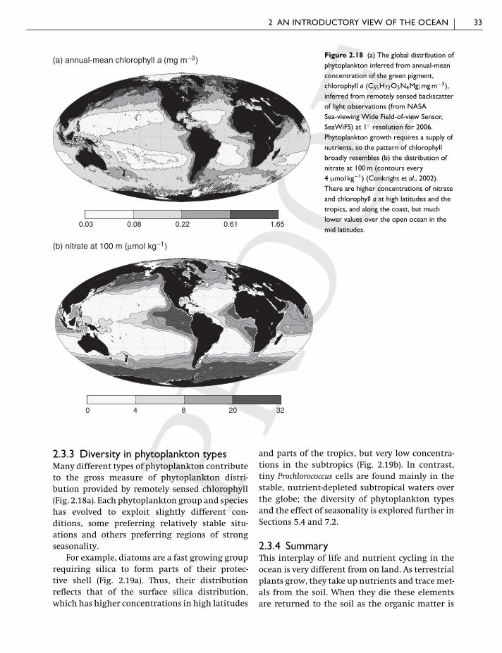
backscattering of green and blue wavelengths, canthen be used to infer the concentration of chloro-phyll and, hence, provide a gross measure of thesurface phytoplankton distribution, as depicted inFig. 2.18a.

Though the incident solar radiation increasestowards the tropics, the highest surface concentra-tions of chlorophyll are in the shelf seas and high-latitude open ocean. Phytoplankton require notonly sunlight, but also inorganic nutrients. Hence,the chlorophyll distribution broadly resemblesthe underlying nitrate distribution, with highconcentrations in the high latitudes, shelf seasand parts of the tropics, and low or depletedconcentrations in the mid latitudes (Fig. 2.18b);this connection is explored further in Sections 7.2and 11.1.


0.03 0.08 0.22 0.61 1.65

(a) annual-mean chlorophyll a (mg m–3)

(b) nitrate at 100 m (μmol kg–1)

0 4 8 20 32

Figure 2.18 (a) The global distribution ofphytoplankton inferred from annual-meanconcentration of the green pigment,chlorophyll a (C55H72O5N4Mg; mg m−3),inferred from remotely sensed backscatterof light observations (from NASASea-viewing Wide Field-of-view Sensor,SeaWiFS) at 1◦ resolution for 2006.Phytoplankton growth requires a supply ofnutrients, so the pattern of chlorophyllbroadly resembles (b) the distribution ofnitrate at 100 m (contours every4 μmol kg−1) (Conkright et al., 2002).There are higher concentrations of nitrateand chlorophyll a at high latitudes and thetropics, and along the coast, but muchlower values over the open ocean in themid latitudes.

2.3.3 Diversity in phytoplankton typesMany different types of phytoplankton contributeto the gross measure of phytoplankton distri-bution provided by remotely sensed chlorophyll(Fig. 2.18a). Each phytoplankton group and specieshas evolved to exploit slightly different con-ditions, some preferring relatively stable situ-ations and others preferring regions of strongseasonality.

For example, diatoms are a fast growing grouprequiring silica to form parts of their protec-tive shell (Fig. 2.19a). Thus, their distributionreflects that of the surface silica distribution,which has higher concentrations in high latitudes

and parts of the tropics, but very low concentra-tions in the subtropics (Fig. 2.19b). In contrast,tiny Prochlorococcus cells are found mainly in thestable, nutrient-depleted subtropical waters overthe globe; the diversity of phytoplankton typesand the effect of seasonality is explored further inSections 5.4 and 7.2.

2.3.4 SummaryThis interplay of life and nutrient cycling in theocean is very different from on land. As terrestrialplants grow, they take up nutrients and trace met-als from the soil. When they die these elementsare returned to the soil as the organic matter is


0 3.75 7.5 15 22.5 30

(b) silicate at 100 m (μmol kg−1)

(a) diatoms

5 μm 10 μm 5 μm

Figure 2.19 (a) Electron micrographsof the silica-based structural parts offossil and modern diatoms (imagescourtesy of Zoe Finkel). There arethousands of species of diatom, spanningseveral orders of magnitude in cell size,some forming chain-like colonies. Theavailability of silicic acid in surface watersshapes their habitat. (b) Climatological,annual silicic acid concentration(μmol kg−1) at a depth of 100 m(Conkright et al., 2002).

respired locally by bacteria, and are assimilatedthe next year, and so the cycle goes on. In theoceans, sunlight is rapidly absorbed with depthand most of the water column is dark. When phy-toplankton grow in the thin, sunlit surface layer,they consume inorganic nutrients. Most of theorganic matter formed in the surface ocean is recy-cled locally, but a small fraction sinks through thewater column, appearing like falling snow. Ulti-mately this organic matter is respired and regen-erates inorganic nutrients at depth. This biologi-cal cycling then acts to transfer nutrients from thesurface to the deep ocean and, ultimately, photo-synthesis ceases unless nutrients can be returnedto the sunlit surface layer. This resupply of nutri-ents to the surface ocean is principally achievedby physical processes acting within the ocean.

2.4 The carbon cycle in the ocean

Carbon dioxide dissolves and reacts in seawaterforming dissolved carbon dioxide, CO∗

2 (defined

by the sum of the aqueous form of carbon diox-ide, COaq

2 , and carbonic acid, H2CO3), bicarbon-ate ions, HCO−

3 , and carbonate ions, CO2−3 , which

collectively are referred to as dissolved inorganiccarbon, DIC:

DIC = [CO∗2] + [HCO−

3 ] + [CO2−3 ], (2.1)

where square brackets denote concentrations inseawater defined per unit mass in μmol kg−1.

While carbon is exchanged between the atmo-sphere and ocean in the form of carbon dioxide,most of the carbon dioxide is transferred intobicarbonate and carbonate ions within the ocean,such that typically 90% of DIC is made up of bicar-bonate ions, about 9% as carbonate ions, and onlya small remainder, up to 1%, as dissolved carbondioxide (Fig. 2.20).

This transfer of carbon dioxide into bicarbon-ate and carbonate ions then leads to the oceanholding 50 times as much carbon as in the over-lying atmosphere. This inorganic carbon in theocean is about 40 times larger than the amountheld as organic carbon.


HCO3−CO2* CO3

2−

at2CO2 = K0 pCOat

DIC

atmosphere

ocean

Figure 2.20 Carbon dioxide dissolves in and reacts withseawater, making up three dissolved inorganic forms of carbon:dissolved carbon dioxide, CO∗

2, bicarbonate, HCO−3 , and

carbonate CO2−3 ions, which together make up dissolved

inorganic carbon, DIC. For the present day, most of thedissolved inorganic carbon is in the form of bicarbonate ions.The air–sea exchange of carbon dioxide depends on thedifference in the dissolved concentration of carbon dioxide inthe ocean and the atmosphere, COat

2 , which is related to thesolubility, K 0, and the partial pressure of carbon dioxide, pCOat

2 .

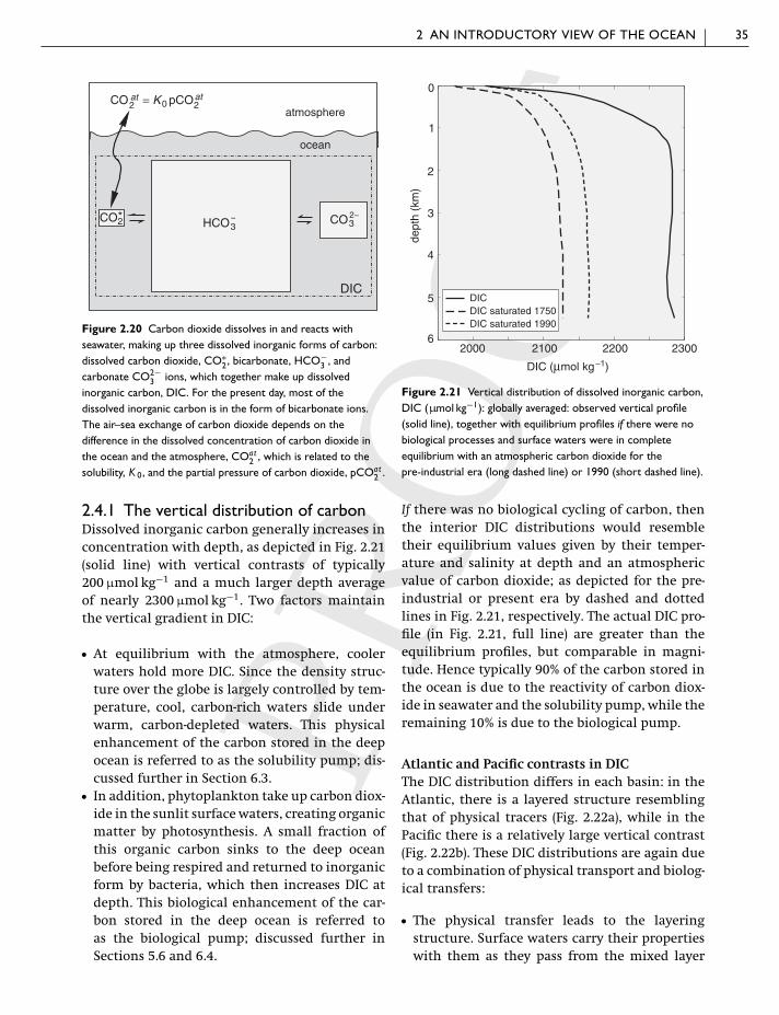
2.4.1 The vertical distribution of carbonDissolved inorganic carbon generally increases inconcentration with depth, as depicted in Fig. 2.21(solid line) with vertical contrasts of typically200 μmol kg−1 and a much larger depth averageof nearly 2300 μmol kg−1. Two factors maintainthe vertical gradient in DIC:

� At equilibrium with the atmosphere, coolerwaters hold more DIC. Since the density struc-ture over the globe is largely controlled by tem-perature, cool, carbon-rich waters slide underwarm, carbon-depleted waters. This physicalenhancement of the carbon stored in the deepocean is referred to as the solubility pump; dis-cussed further in Section 6.3.

� In addition, phytoplankton take up carbon diox-ide in the sunlit surface waters, creating organicmatter by photosynthesis. A small fraction ofthis organic carbon sinks to the deep oceanbefore being respired and returned to inorganicform by bacteria, which then increases DIC atdepth. This biological enhancement of the car-bon stored in the deep ocean is referred toas the biological pump; discussed further inSections 5.6 and 6.4.

2000 2100 2200 2300

DIC (μmol kg–1)

0

1

2

3

4

5

6

dept

h (k

m)

DIC saturated 1750DIC saturated 1990

DICDIC saturated 1750DIC saturated 1990

DIC

Figure 2.21 Vertical distribution of dissolved inorganic carbon,DIC (μmol kg−1): globally averaged: observed vertical profile(solid line), together with equilibrium profiles if there were nobiological processes and surface waters were in completeequilibrium with an atmospheric carbon dioxide for thepre-industrial era (long dashed line) or 1990 (short dashed line).

If there was no biological cycling of carbon, thenthe interior DIC distributions would resembletheir equilibrium values given by their temper-ature and salinity at depth and an atmosphericvalue of carbon dioxide; as depicted for the pre-industrial or present era by dashed and dottedlines in Fig. 2.21, respectively. The actual DIC pro-file (in Fig. 2.21, full line) are greater than theequilibrium profiles, but comparable in magni-tude. Hence typically 90% of the carbon stored inthe ocean is due to the reactivity of carbon diox-ide in seawater and the solubility pump, while theremaining 10% is due to the biological pump.

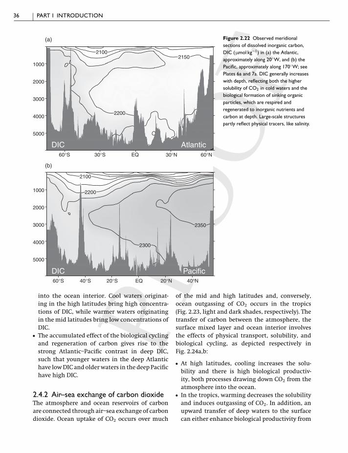
Atlantic and Pacific contrasts in DICThe DIC distribution differs in each basin: in theAtlantic, there is a layered structure resemblingthat of physical tracers (Fig. 2.22a), while in thePacific there is a relatively large vertical contrast(Fig. 2.22b). These DIC distributions are again dueto a combination of physical transport and biolog-ical transfers:

� The physical transfer leads to the layeringstructure. Surface waters carry their propertieswith them as they pass from the mixed layer


2200

21502100

2350

2300

2100

2200

60°S 30°S EQ 30°N 60°N

5000

4000

3000

2000

1000

(a)

AtlanticDIC

60°S 40°S 20°S EQ 20°N 40°N

5000

4000

3000

2000

1000

PacificDIC

(b)

Figure 2.22 Observed meridionalsections of dissolved inorganic carbon,DIC (μmol kg−1) in (a) the Atlantic,approximately along 20◦W, and (b) thePacific, approximately along 170◦W; seePlates 6a and 7a. DIC generally increaseswith depth, reflecting both the highersolubility of CO2 in cold waters and thebiological formation of sinking organicparticles, which are respired andregenerated to inorganic nutrients andcarbon at depth. Large-scale structurespartly reflect physical tracers, like salinity.

into the ocean interior. Cool waters originat-ing in the high latitudes bring high concentra-tions of DIC, while warmer waters originatingin the mid latitudes bring low concentrations ofDIC.

� The accumulated effect of the biological cyclingand regeneration of carbon gives rise to thestrong Atlantic–Pacific contrast in deep DIC,such that younger waters in the deep Atlantichave low DIC and older waters in the deep Pacifichave high DIC.

2.4.2 Air–sea exchange of carbon dioxideThe atmosphere and ocean reservoirs of carbonare connected through air–sea exchange of carbondioxide. Ocean uptake of CO2 occurs over much

of the mid and high latitudes and, conversely,ocean outgassing of CO2 occurs in the tropics(Fig. 2.23, light and dark shades, respectively). Thetransfer of carbon between the atmosphere, thesurface mixed layer and ocean interior involvesthe effects of physical transport, solubility, andbiological cycling, as depicted respectively inFig. 2.24a,b:

� At high latitudes, cooling increases the solu-bility and there is high biological productiv-ity, both processes drawing down CO2 from theatmosphere into the ocean.

� In the tropics, warming decreases the solubilityand induces outgassing of CO2. In addition, anupward transfer of deep waters to the surfacecan either enhance biological productivity from


annual-mean CO2 flux (mol m−2 y−1)

−7.5 −5 −2.5 0 2.5 5 7.5

Figure 2.23 Climatological, annual-meanmap of air–sea flux of CO2 into the ocean(mol m−2 y−1), data from Takahashi et al.(2002). There is an ocean uptake of CO2

(light shading) in the high latitudes and anocean outgassing in the tropics (darkshading); however, there is considerableuncertainty in the direction of the fluxover the Southern Ocean. This estimate isbased on a compilation of about a millionmeasurements of surface-water pCO2

obtained since the InternationalGeophysical Year of 1956–59. Theclimatology represents mean non-El Ninoconditions with a spatial resolution of4◦ × 5◦, normalised to reference year1995.

atmosphere

mixedlayer

ocean interior

uptakeoutgassing

CO2 CO2CO2 CO2

warming cooling

atmosphere

mixerlayer

ocean interior

biologicalfallout

outgassing biologicaldrawdown

(a) physical transport and solubility (b) physical transport and biology

entrainment ofcarbon-rich waters

respiration and regeneration

physical transfer from surface to interior

physical transfer from interior to surface

Figure 2.24 A schematic figure depicting how air–sea exchange of CO2 is affected by an interplay of physical and biologicalprocesses involving the cycling and transport of DIC. In (a), warming of surface waters leads to an outgassing of CO2, while a coolingof surface waters leads to an ocean uptake of CO2. The physical transport (thick black arrows) of surface waters into the interior isthen associated with an uptake of CO2, while the return of deep waters to the surface leads to an outgassing of CO2. In (b), thebiological formation of organic matter leads to an ocean drawdown of atmospheric CO2, which is then transferred to the oceaninterior through the fallout of organic matter (white arrow). The respiration of the organic matter then regenerates the inorganicnutrients and carbon, increasing their concentrations in the deep waters. The return of deep water to the surface leads to anoutgassing of CO2.

the supply of nutrient-rich waters leading to anocean uptake of CO2 or, conversely, the supplyof carbon-rich waters can lead to an outgassingof CO2.

The air–sea fluxes of carbon dioxide integratedover the separate outgassing and uptake regionsof the globe approximately balance each other,typically reaching 90 Pg C y−1 in each direction

(based upon Fig. 2.23). In comparison, the anthro-pogenic increase in atmospheric CO2 leads to a netair–sea flux directed into the ocean of 2 Pg C y−1,much smaller than the regional variations in theannual flux. This anthropogenic increase may,though, tip the balance over parts of the South-ern Ocean, possibly changing a pre-industrialnet outgassing to a present-day or futureuptake.


2.5 Summary

This chapter provides a preliminary view of theopen ocean. The ocean circulation is driven bymechanical forcing from the surface winds andtides, as well as by pressure gradients from densitydifferences formed through surface exchanges ofheat, fresh water and salt. The ocean circulationcan be viewed in terms of a horizontal circula-tion confined between the continents, made upof recirculating gyres and western boundary cur-rents, together with intense, near-zonal currentsrunning along the equator and circumnavigat-ing the Southern Ocean. In addition, there is avertical overturning with dense water sinking athigh latitudes, especially in the North Atlantic andSouthern Ocean, spreading over the globe at depthand replaced by lighter surface waters from lowerlatitudes.

The imprint of the physical circulation is seenin how a range of physical and biogeochemicalproperties resemble each other: plumes of freshand nutrient-rich water spread northward fromthe Southern Ocean and the thickness of the rela-tively warm and nutrient-depleted, thermoclinewaters undulate together; as illustrated in themeridional sections in colour plates 2 to 6.

Phytoplankton absorb visible wavelengths oflight and use the energy, along with nutrients con-taining essential elements, to create new organicmolecules or reproduce by producing a copy ofthe cell. The organic matter provides the ultimatesource of energy and nutrients for all other liv-ing creatures in the ocean. Phytoplankton growthleads to the consumption of inorganic nutrients insurface waters; some of the organic matter grav-itationally sinks through the water column andis respired to regenerate inorganic nutrients atdepth.

Carbon is stored within the ocean predomi-nantly as dissolved inorganic carbon, consistingmainly of bicarbonate and carbonate ions withless than one per cent held as dissolved carbondioxide. The ocean inventory of carbon is typicallyfifty times larger than the atmospheric inventoryof carbon dioxide.

Carbon dioxide is exchanged between theatmosphere and ocean: the ocean takes up carbon

dioxide when surface waters cool and sink, andwhen phytoplankton grow, forming new organicmatter. Conversely, carbon dioxide is returned tothe atmosphere when surface waters warm andwhen carbon and nutrient-rich deep waters arereturned to the surface. Carbon is transferred intothe ocean interior by the physical transfer of cold,carbon-rich surface waters and by the biologicaltransfer of organic matter, falling through thewater column and being respired at depth.

Following this descriptive overview, thesethemes are taken forward in a set of fundamen-tal chapters addressing the controlling processesin more detail: how tracers are transported by thecirculation; how the ocean circulates and is forcedby the atmosphere; how phytoplankton cells growand their implications for biogeochemistry; andhow carbon dioxide is cycled in the ocean andexchanged with the atmosphere.

2.6 Questions

Q2.1. Heat storage of the atmosphere and ocean.

Estimate the thickness of the ocean that holds asmuch heat as the overlying atmosphere, where theamount of heat Q required to raise the tempera-ture of the atmosphere or ocean by �T is given by,

Q = ρC p AD�T , (2.2)

where ρ is density (kg m−3), C p is heat capacity(J kg−1 K−1), A is horizontal area (m2), and D is thevertical scale (m).

Assume ρ ∼ 1 kg m−3 for the atmosphere and103 kg m−3 for the ocean, C p ∼ 1000 J kg−1 K−1 forthe atmosphere and 4000 J kg−1 K for the ocean,a vertical scale, D, of 10 km for the atmosphere(where the bulk of the atmosphere resides), �T =1 K and a horizontal area A = 1 m2.

Q2.2. Radiative heating and equilibrium temperature.

(a) For a planet with no atmosphere, derivehow the equilibrium temperature, T , in kelvin,depends on the incident solar radiation, Sc , andthe albedo, α, the fraction of reflected sunlight,

T =(

(1 − α)Sc

4σsb

)1/4

, (2.3)


planet

RR

net incoming solar radiationflux per unit area, Sc (1-α)

outgoing long-wave radiationflux per unit area, σsbT4

cross-sectionalarea, πR2

surfacearea, 4πR2

Figure 2.25 A schematic figure of the netincident solar radiation per unit horizontal area,the incident minus the reflected, Sc (1 − α),which is absorbed over the cross-sectional areaof a planet with radius R . The outgoing long-waveradiation, σsb T 4, is radiated over the entiresurface area of the planet.

where σsb is the Stefan-Boltzmann constant.Assume a radiative balance, as depicted inFig. 2.25, where (i) the net solar radiation isabsorbed over a circular disc with a cross-sectionalarea of the planet, and (ii) the outgoing long-waveradiation per unit horizontal area in W m−2 isgiven by the Stefan-Boltzmann law, σsbT 4, inte-grated over the surface area of the planet.

(b) Estimate this equilibrium temperature inkelvin for Venus, Earth and Mars assuming thatSc is 2600, 1400 and 590 W m−2, and their albe-dos, α, are 0.8, 0.3 and 0.15, respectively, andσsb = 5.7 × 10−8 W m−2 K−4. How do these temper-atures compare with their respective observed sur-face values of typically 750 K, 280 K and 220 K? Whymight there be a mismatch in some cases?

(c) If the planet is now assumed to have anatmosphere that is transparent to solar radiation,but absorbs and re-radiates long-wave radiation,then a local radiative balance suggests that theabsorbed solar and long-wave radiation at theground balances the outgoing long-wave radia-tion. The surface temperature is then given by

T =(

(1 − α)Sc

2σsb

)1/4

. (2.4)

Use this relationship to estimate the impliedtemperature contrast between the tropics andthe high latitudes. For simplicity, in the tropics,assume that the incident radiation is given by Sc ,while at the high latitudes, the incident radiationis given by Sc/3. How does this estimate comparewith the actual meridional temperature contrastof typically 30 K for the Earth?

Q2.3. Anthropogenic heating of the ocean by the increasein atmospheric CO2.

Increasing atmospheric CO2 leads to increasingradiative heating, �H (in W m−2), which varieslogarithmically with the increase in mixing ratiofor atmospheric CO2 (as the effect of increasingCO2 on the absorption and emission of long-waveradiation gradually saturates),

�H = αr ln (XCO2 (t)/XCO2 (t0)) , (2.5)

where αr = 5.4 W m−2 depends on the chemicalcomposition of the atmosphere and XCO2 (t0) andXCO2 (t) are the mixing ratios for CO2 at timest0 to t.

(a) Estimate the increase in implied radiative heat-ing, �H, over the 50 years between 1958 and 2008assuming an increase in XCO2 from 315 ppmv to386 ppmv; compare your answer with Fig. 1.11b.

(b) Given these estimates of radiative heating, thenestimate how much the upper ocean might warmover 50 years. Assume that the temperature riseof the ocean is given from a simple heat balanceby

�T ∼ �H t

ρC ph,

where �H is the average extra heating over thetime period, t, of 50 years (convert to seconds) andh is the thickness of the upper ocean, taken as1000 m; ρ and C p are as in Q2.1. Compare thisestimate with the reported change for the globalwarming of the Earth over the last 50 years (IPCC,2007).


Earth’s rotation, Ω

radius, R

φ

R cos φu > 0

tube of airencircling Earth

equator

pole

u = 0

Figure 2.26 A schematic figure depicting a tube of air (darkshading) encircling the Earth along a latitude circle with theEarth rotating at an angular velocity �. The tube is at a distanceR cos φ from the rotational axis where R is the radius and φ isthe latitude. As the tube moves from the equator towards thepole, the tube increases its zonal velocity, u , so as to conserveangular momentum. Adapted from Green (1981).

Q2.4. Atmospheric zonal jets and angular momentum.

Consider a tube of air circling the Earth at itsequator that is uniformly displaced poleward, asdepicted in Fig. 2.26. The angular momentum ofthe tube is given by

Lang = (u + �R cos φ) R cos φ, (2.6)

where u is the zonal velocity, � is the angularvelocity, R is the radius of the Earth, and φ is thelatitude. R cos φ represents the effective radius ofthe tube to its rotational axis, �R cos φ representsthe velocity of the spinning Earth relative to afixed point in space and u represents the velocityof the air relative to the Earth.

(a) Derive an expression giving the zonal velocity,u, as a function of latitude, φ, by assuming thatangular momentum Lang is conserved and the ini-tial zonal velocity at the equator is zero.

(b) Calculate the implied zonal velocity for every10◦ from the equator to 30◦N for the Earth, assum-ing � = 2π/day and R = 6340 km. What are theimplications of your result?

2.7 Recommended reading

A descriptive view of the ocean circulation is providedin L. D. Talley, G. L. Pickard, W. J. Emery and J. H.Swift, Descriptive Physical Oceanography: An Introduction.6th edition, Academic Press (due for publication2011).

A comprehensive view of the ocean, includingobservations, theory and modelling, is provided inG. Siedler, J. Church and J. Gould (2001). OceanCirculation and Climate: Observing and Modelling theGlobal Ocean. San Diego, CA: Academic Press, 693pp.

An introductory view of the physical processesoperating in the atmosphere and ocean, drawing onlaboratory experiments and relevant theory, isprovided by J. Marshall and R. A. Plumb (2008).Atmosphere, Ocean and Climate Dynamics: AnIntroductory Text. Burlington, MA: Academic PressElsevier, 319pp.

An introductory view of marine chemical processes isprovided by S. Emerson and J. Hedges (2008). ChemicalOceanography and the Marine Carbon Cycle. Cambridge:Cambridge University Press, 468pp.

An advanced view of the biogeochemistry and carboncycle is provided by J. L. Sarmiento and N. Gruber(2006). Ocean Biogeochemical Dynamics. Princeton, NJ:Princeton University Press, 526pp.

an introductory view of the ocean

Documents