an investigation in construction cost estimation using a
TRANSCRIPT
Air Force Institute of TechnologyAFIT Scholar
Theses and Dissertations Student Graduate Works
6-16-2016
An Investigation in Construction Cost EstimationUsing a Monte Carlo SimulationJeffrey D. Buchholtz
Follow this and additional works at: https://scholar.afit.edu/etd
Part of the Construction Engineering and Management Commons
This Thesis is brought to you for free and open access by the Student Graduate Works at AFIT Scholar. It has been accepted for inclusion in Theses andDissertations by an authorized administrator of AFIT Scholar. For more information, please contact [email protected].
Recommended CitationBuchholtz, Jeffrey D., "An Investigation in Construction Cost Estimation Using a Monte Carlo Simulation" (2016). Theses andDissertations. 281.https://scholar.afit.edu/etd/281
AFIT-ENV-MS-16-M-137
AN INVESTIGATION IN CONSTRUCTION COST ESTIMATION USING A
MONTE CARLO SIMULATION
THESIS
Jeffrey D. Buchholtz, Captain, USAF
AFIT-ENV-MS-16-M-137
DEPARTMENT OF THE AIR FORCE AIR UNIVERSITY
AIR FORCE INSTITUTE OF TECHNOLOGY
Wright-Patterson Air Force Base, Ohio
DISTRIBUTION STATEMENT A. APPROVED FOR PUBLIC RELEASE;
DISTRIBUTION UNLIMITED.

AFIT-ENV-MS-16-M-137
The views expressed in this thesis are those of the author and do not reflect the official
policy or position of the United States Air Force, Department of Defense, or the United
States Government. This material is declared a work of the United States Government
and is not subject to copyright protection in the United States.
AFIT-ENV-MS-16-M-137
AN INVESTIGATION IN CONSTRUCTION COST ESTIMATION USING A MONTE
CARLO SIMULATION
THESIS
Presented to the Faculty
Department of Systems Engineering and Management
Graduate School of Engineering and Management
Air Force Institute of Technology
Air University
Air Education and Training Command
In Partial Fulfillment of the Requirements for the
Degree of Master of Science in Engineering Management
Jeffrey D. Buchholtz, BS
Captain, USAF
March 2016
DISTRIBUTION STATEMENT A. APPROVED FOR PUBLIC RELEASE;
DISTRIBUTION UNLIMITED.

AFIT-ENV-MS-16-M-137
AN INVESTIGATION IN CONSTRUCTION COST ESTIMATION USING A MONTE
CARLO SIMULATION
Jeffrey D. Buchholtz, BS
Captain, USAF
Committee Membership:
Maj Gregory D. Hammond, PhD
Chair
Lt Col Christopher M. Stoppel, PhD
Member
Robert D. Fass, PhD
Member
AFIT-ENV-MS-16-M-137
iv
Abstract
The Air Force estimates military construction (MILCON) costs early in a
project’s development as a part of the funding approval process. However, many of the
initial cost estimates deviate significantly more than expected from the actual project
costs, hindering funding allocation efforts. There is a need for improved estimation
techniques. This research examines a cost estimation model for the initial programming
stages of a project when only general scope information is available.
This study develops a Monte Carlo simulation based on historical construction
cost data to predict project costs base on facility type. For a given facility type, the
research identified distributions and associated correlations to model major cost elements
from the historical data. The Monte Carlo simulation uses these distributions and
correlations to estimate the total cost of separate validation projects. The results reveal a
histogram, showing the probability range of possible costs for each project. This research
compares these results to the actual costs and cost estimates for the same projects along
with additional estimated costs derived from standard Air Force cost estimation guides.
The results highlight the level of accuracy for current estimation techniques and validate
the utility of this model. The Air Force can use this model to improve initial cost
estimates, better predicting expected costs in addition to revealing the uncertainty
inherent in those costs.

v
Acknowledgments
I am most grateful for my beautiful wife and daughter who supported me
throughout this entire thesis effort. Their encouragement and affirmation was invaluable.
I would also like to express my gratitude to my research advisor, Maj Greg
Hammond, for his guidance throughout this journey. The classroom instruction and
insights along the way, along with those of Lt Col Stoppel and Dr. Fass on my
committee, aided this effort.
This thesis would also not be possible without the aid of many who helped me
track down the information and data required. My sponsors at AFCEC, including Mr.
Tim Sullivan and Mr. Ben Kindt, along with Mr. Ron Davis and Mr. Jim Winslow,
provided me with much-needed insight into Air Force historical cost estimation and the
project data the Air Force records. In addition, Ms. Ann Rea with the U.S. Army Corps
of Engineers proved to be the vital link to the Army’s construction data necessary for me
to complete this work.
Thank you all for your support.
Jeffrey D. Buchholtz

vi
Table of Contents
Page
Abstract .............................................................................................................................. iv
Acknowledgments................................................................................................................v
List of Figures .................................................................................................................... ix
List of Tables .......................................................................................................................x
I. Introduction .....................................................................................................................1
Background .....................................................................................................................1 Problem Statement ..........................................................................................................3 Research Objectives/Questions/Hypotheses ...................................................................3 Scope and Methodology ..................................................................................................4 Significance .....................................................................................................................6
II. Literature Review ...........................................................................................................8
Chapter Overview ...........................................................................................................8 Cost Estimation Framework ............................................................................................8 Current State of Industry Construction Cost Estimation.................................................9
Cost Point Estimation ................................................................................................ 9 Cost Contingency Estimation .................................................................................. 11 Summary .................................................................................................................. 13
Current State of Air Force Construction Cost Estimation ............................................14 Unified Facilities Criteria Cost Estimation Methods ............................................. 14 Summary .................................................................................................................. 20
The Monte Carlo Method ..............................................................................................21 Development for Construction Applications ........................................................... 22 Monte Carlo Improvements ..................................................................................... 22
Conclusion ....................................................................................................................23
III. Methodology ...............................................................................................................25
Chapter Overview .........................................................................................................25 Monte Carlo Simulation ................................................................................................25 Data Collection..............................................................................................................27 Cost Element Selection .................................................................................................28 Distribution Characterization ........................................................................................31 Correlation Characterization .........................................................................................35 Validation Process .........................................................................................................36
UFC Estimate Comparison ..................................................................................... 38 AFCESA Estimate Comparison ............................................................................... 39
vii
Summary .......................................................................................................................40
IV. Analysis and Results ...................................................................................................41
Chapter Overview .........................................................................................................41 Methodology Implementation .......................................................................................41
Data Collection ....................................................................................................... 42 Cost Element Categorization .................................................................................. 43 Cost Element Standardization ................................................................................. 45 Distribution Modeling ............................................................................................. 46 Correlation Modeling .............................................................................................. 47 Simulation Modeling ............................................................................................... 48
Model Validation ..........................................................................................................49 Dormitory Project Cost Estimation ......................................................................... 51 Education and Training Project Cost Estimation ................................................... 53 Squadron Operations Project Cost Estimation ....................................................... 55
Investigative Questions Answered ................................................................................59 Question 1 ............................................................................................................... 59 Question 2 ............................................................................................................... 60 Question 3 ............................................................................................................... 60
Summary .......................................................................................................................62
V. Conclusions and Recommendations ............................................................................63
Chapter Overview .........................................................................................................63 Conclusions of Research ...............................................................................................63 Limitations of Research ................................................................................................64 Significance of Research ...............................................................................................65 Recommendations for Action .......................................................................................65 Recommendations for Future Research ........................................................................66 Summary .......................................................................................................................67
Appendix A: Construction Cost Research White Paper ....................................................69
I. Overview ..................................................................................................................70 II. Research ...................................................................................................................70
1. Historical Cost Trend Analyses ........................................................................ 70 2. Parametric Estimation Models ......................................................................... 74 3. Contract Method Evaluations .......................................................................... 76 4. Program-Wide MILCON Investigations .......................................................... 78
Appendix A-1: Abstracts .............................................................................................81
Appendix B: Supplemental Data and Analysis Results .....................................................89
Project Data Set with Total and Unit Cost Element Amounts ......................................89 Cost Element Data Characteristics and Distribution Selection .....................................95
viii
Education & Training Cost Distribution Fitting ..................................................... 95 Dormitory Cost Distribution Fitting ....................................................................... 99 Squadron Operations Cost Fitting ........................................................................ 103
Final Cost Element Generalized Beta Distribution Parameters ..................................107 Cost Element Distribution Kolmogorov-Smirnov GoF Test Results .........................108 Cost Element Correlation Matrices by Facility Type .................................................109 Comparison Cost Estimates from UFC and AFCESA ................................................111
Appendix C: Line Item Key Word Coding ......................................................................112
Appendix D: Cost Estimate Comparisons .......................................................................115
Appendix E: Model Code from R ....................................................................................116
Bibliography ....................................................................................................................138

ix
List of Figures
Page
Figure 1: AACE Cost Estimate Classification Matrix (Christensen & Dysert, 2011) ...... 10
Figure 2: Cullen & Frey Graph of Mechanical Costs in Squadron Operations Facilities 34
Figure 3: Lackland ATC Dormitory Simulation Results and Cost Estimate Comparison
................................................................................................................................... 52
Figure 4: Whiteman CDC Simulation Results and Cost Estimate Comparisons............. 54
Figure 5: Eielson Chapel Simulation Results and Cost Estimate Comparisons .............. 55
Figure 6: Hanscom Acquisition Management Facility Simulation Results and Cost
Estimate Comparisons ............................................................................................... 56
Figure 7: Kirtland AFNWC Sustainment Center Simulation Results and Cost Estimate
Comparisons .............................................................................................................. 58
Figure 8: Accuracy Comparison between Cost Estimates ............................................... 59
x
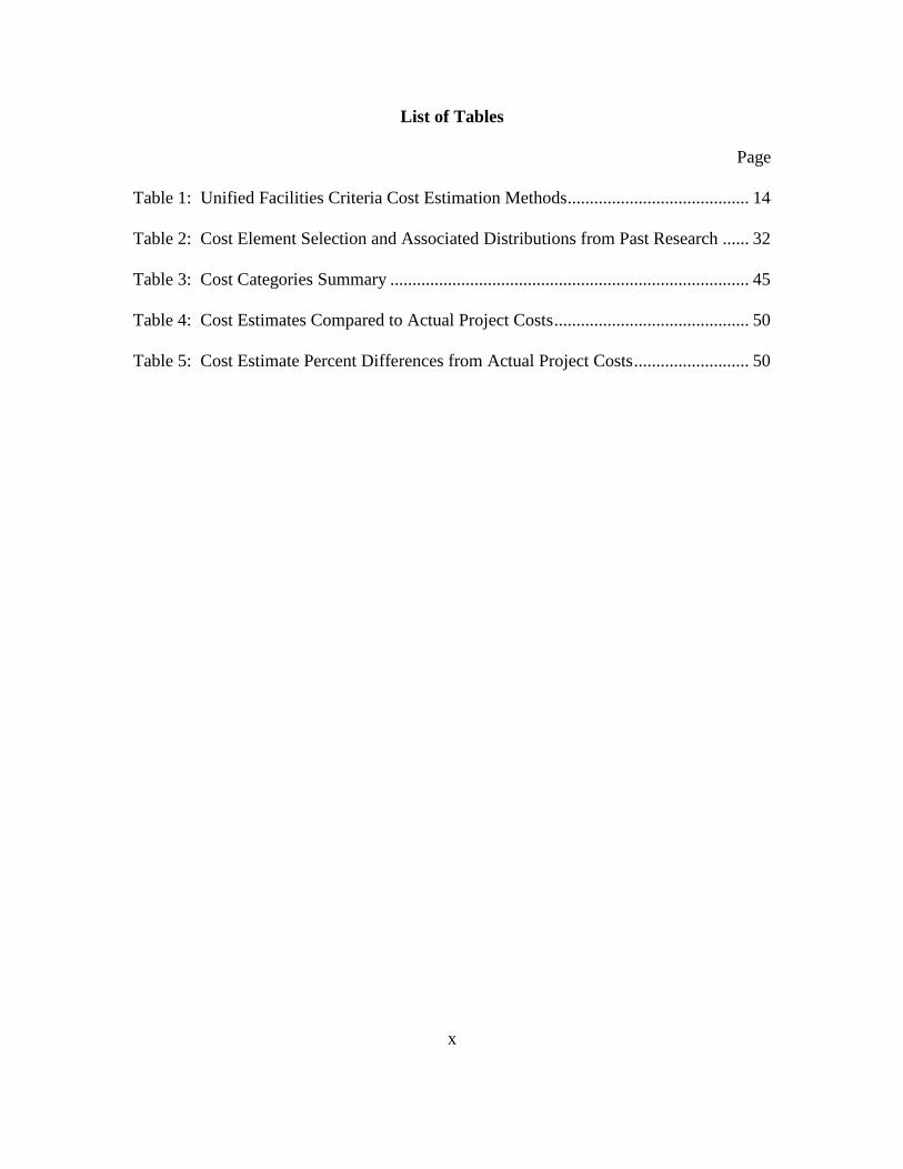
List of Tables
Page
Table 1: Unified Facilities Criteria Cost Estimation Methods ......................................... 14
Table 2: Cost Element Selection and Associated Distributions from Past Research ...... 32
Table 3: Cost Categories Summary ................................................................................. 45
Table 4: Cost Estimates Compared to Actual Project Costs ............................................ 50
Table 5: Cost Estimate Percent Differences from Actual Project Costs .......................... 50

1
AN INVESTIGATION IN CONSTRUCTION COST ESTIMATION USING A MONTE
CARLO SIMULATION
I. Introduction
Background
Military Construction (MILCON) project cost estimates are heavily scrutinized
items within the Department of Defense with demanding requirements for detail and
accuracy (U.S. Government Accountability Office, 2009). This scrutiny is no surprise
given the emphasis on reducing costs and the lengthy approval process for MILCON
projects (Air Force Center for Engineering and the Environment, 2007). In response, the
Air Force, along with the other military branches, has turned to a set of cost estimation
principles outlined in the Unified Facilities Criteria (UFC) to optimize cost estimation.
The UFC summarizes the spectrum of construction activities with specific guides
for cost estimation. Using these guides, Air Force civil engineers, and United States
Army Corps of Engineers (USACE) personnel create various cost estimates for
construction projects to adequately predict costs for programming and planning purposes.
The DoD Facilities Pricing Guide provides principles for deriving the first cost estimate
used for general scoping of a project by outlining broad cost factors for categories such as
facility type and location (Department of Defense, 2015). However, this is just a
preliminary estimate and is expected to be accurate only to within -15% to 25%
(Department of Defense, 2011a). The next phase of estimation is to develop a
parametric cost estimate using system groupings and assemblies to compile a single
expected value, anticipated to be within -10% to +15% of the actual cost (Department of

2
Defense, 2011a). Finally, by dividing the project into as small of work increments as
possible, a Quantity Take Off estimate can be constructed with an expected accuracy of -
7.5% to +10% (Department of Defense, 2011a). Increasing levels of project detail are
required for each phase of cost estimation, relying on increasingly detailed designs.
Therefore, a basic design concept is typically needed before conducting a parametric cost
estimate; and the Quantity Take Off estimate requires a 35% design effort (Department of
Defense, 2011a). The military uses these cost estimation methods throughout the
construction planning process in all the services, and they are derived from the
Association for the Advancement of Cost Engineering’s (AACE) recommended practices
(Department of Defense, 2011a). Each of these methods results in a single point estimate
with a contingency amount, typically 5% added on top of the cost to cover uncertainty.
However, point estimates have inherent problems. First, the point estimates are
compilations of average itemized values that, when summed, tend to create estimates that
underpredict the actual value by underestimating the risks in a project (Willmer, 1991, p.
1155). As stated by Savage: “plans based on average assumptions are wrong on
average” (2012, p. 11). Additionally, simply adding a contingency percentage on top of
average estimates does not produce optimal results. Such a practice typically
underestimates the additional funds required for complex or poorly defined projects
(Burroughs & Juntima, 2004). Even without an overly complex or poorly defined
project, a fixed contingency percent will still be frequently inaccurate because it is simply
a set estimate meant to cover a range of actual contingency values.
3
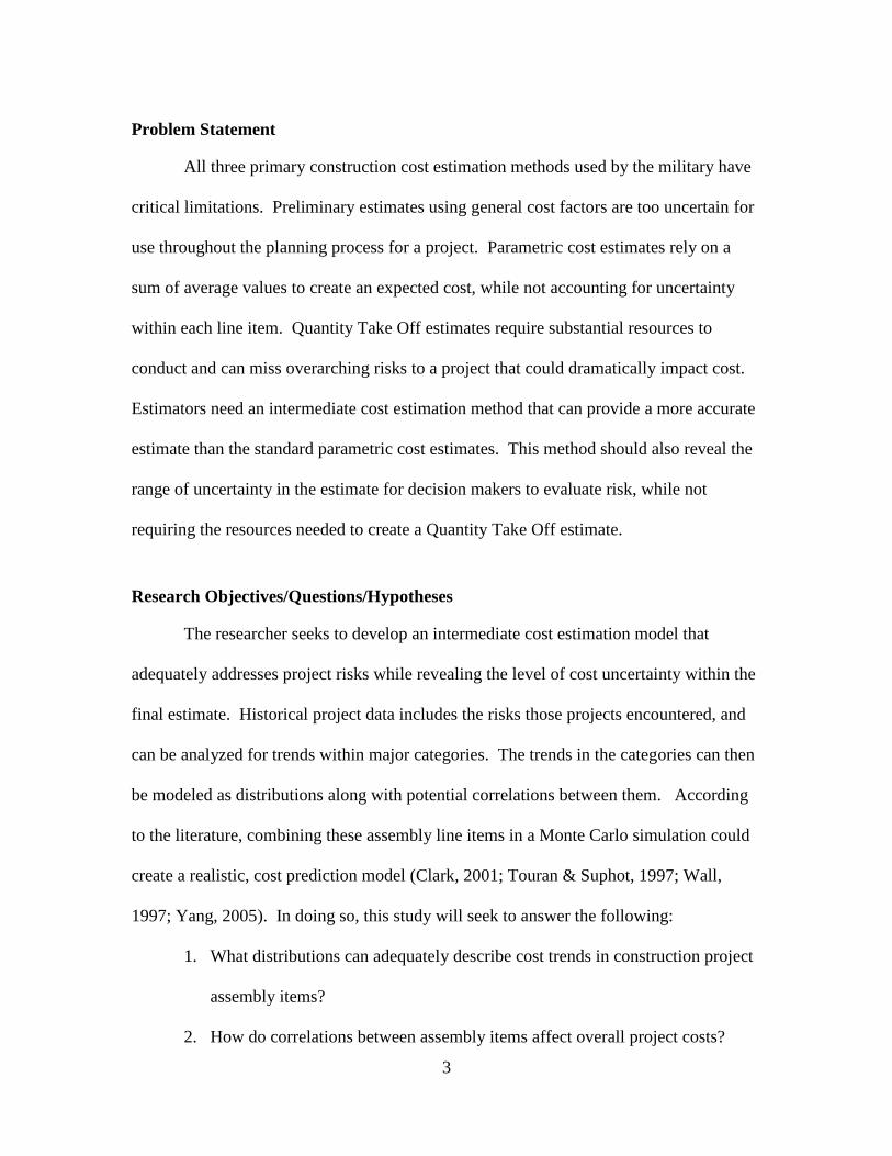
Problem Statement
All three primary construction cost estimation methods used by the military have
critical limitations. Preliminary estimates using general cost factors are too uncertain for
use throughout the planning process for a project. Parametric cost estimates rely on a
sum of average values to create an expected cost, while not accounting for uncertainty
within each line item. Quantity Take Off estimates require substantial resources to
conduct and can miss overarching risks to a project that could dramatically impact cost.
Estimators need an intermediate cost estimation method that can provide a more accurate
estimate than the standard parametric cost estimates. This method should also reveal the
range of uncertainty in the estimate for decision makers to evaluate risk, while not
requiring the resources needed to create a Quantity Take Off estimate.
Research Objectives/Questions/Hypotheses
The researcher seeks to develop an intermediate cost estimation model that
adequately addresses project risks while revealing the level of cost uncertainty within the
final estimate. Historical project data includes the risks those projects encountered, and
can be analyzed for trends within major categories. The trends in the categories can then
be modeled as distributions along with potential correlations between them. According
to the literature, combining these assembly line items in a Monte Carlo simulation could
create a realistic, cost prediction model (Clark, 2001; Touran & Suphot, 1997; Wall,
1997; Yang, 2005). In doing so, this study will seek to answer the following:
1. What distributions can adequately describe cost trends in construction project
assembly items?
2. How do correlations between assembly items affect overall project costs?
4
3. How does a Monte Carlo cost simulation model using historical cost
distributions differ in performance from the current parametric cost estimation
method?
Scope and Methodology
The first phase of this research encompasses data collection and analysis. The
researcher will compile project cost data from Air Force projects completed since 2000,
obtained from the Air Force Civil Engineer Center (AFCEC). Then, through statistical
analysis of the major work sections, the researcher will assign distributions to each
element using best-fit analysis techniques. The data will also be analyzed for
correlations between the elements.
Once element distributions and correlations have been determined, the second
phase of research will develop a Monte Carlo simulation with the distributions as inputs.
A Monte Carlo simulation is ideal for this situation because of its ability to combine
easily numerous distributions with varying properties. This has been done successfully
for many large projects by Honeywell Performance Polymers and Chemicals and cited as
an industry best practice (Clark, 2001). The Government Accountability Office further
encouraged the use of Monte Carlo techniques, emphasizing that point estimates are
unable to reveal program risk while the Monte Carlo method has the benefit of capturing
positive and negative effects and their combination throughout the elements of a project,
therefore improving analysis of the costs (2009, p. 172).
However, the Monte Carlo method is not without potential limitations. Creation
of a Monte Carlo model can be a complex and time-consuming endeavor, making the
process infeasible if it must be re-accomplished for each project (Sonmez, Ergin, &

5
Birgonul, 2007). The amount of effort employed by Honeywell Performance Polymers
and Chemicals emphasizes this limitation, putting a group of up to 30 people through an
effort as long as three days to produce a single project-specific model (Clark, 2001).
Hollmann goes into further detail on the limitations of the Monte Carlo method, noting
the typical lack of dependencies and correlations between line items and the lack of
global risk drivers in the calculations, resulting in an unreliable model (Hollmann, 2007).
The lack of global risk drivers in the model becomes of even greater concern when the
project is complex or poorly defined (Burroughs & Juntima, 2004). Cost estimating for
Air Force construction projects is particularly vulnerable to these limitations because of
the often poor project scoping and limited time spent on planning, as noted in several Air
Force research efforts (Dutcher, 1986; Gannon, 2011; Nielsen, 2007).
To mitigate these limitations, the Monte Carlo simulation in this study will rely on
historical project cost distributions as mentioned previously. Pre-establishing cost
distributions within the model eliminates the need for a group of experts to determine
individual line item distributions for each project. If the cost distributions continue to be
updated and refined as projects finish, the model will continually improve and be easily
used by cost estimators, as was shown by Mulholland and Christian in their study to
develop better construction schedule estimates (1999). Additionally, by including
correlations between the cost distributions, the model can adequately address internal
effects between those costs. Finally, the use of historical data removes subjective
evaluation of the risks involved. Historical cost data includes all the risks those projects
encountered during construction. Therefore, both line item-specific risks and global risks
6
are covered if the appropriate correlations are modeled accurately, addressing the
limitations cited by Hollmann (2007).
Validation of the model includes generating cost estimates for a random sample of
projects withheld from the data analysis phase. The researcher can then compare the
results to the parametric estimates previously completed for those same projects. A
difference in means statistical test will then disclose any differences in cost estimates,
revealing improvements, or lack thereof, to current estimation methods.
Significance
Establishing an accurate, programmed amount for a construction project cost is an
essential part of the MILCON approval process. However, there is no proven method
consistently obtaining the accuracy needed to avoid issues after the project is approved
and the magnitude of the estimate errors become known. Estimators establish the
programmed amount during the initial project programming phase before an Architect
and Engineering (A&E) firm or other agency can do a detailed line item estimate as a part
of a design effort (Air Force Center for Engineering and the Environment, 2007).
However, if a design effort, later on, indicates the project will cost more than 25% above
the programmed amount, the project may have to be reprogrammed, and the approval
process started from the beginning (Air Force Center for Engineering and the
Environment, 2007). Even if the project remains within 25% of the original estimate, the
extent to which the estimate is inaccurate creates funding ripple effects of shortages or
excesses that programmers must address throughout the MILCON program. The
development of a cost estimation model that would provide increased accuracy but still
7
be feasible to use before a project’s detailed design phase could significantly mitigate
these risks.
8
II. Literature Review
Chapter Overview
Construction cost estimation includes uncertainty, and past research has
developed numerous methods to address varying types of uncertainty. Typically, these
uncertainties are grouped into either systemic or project-specific categories, the former
representing predictable uncertainties for which plans can be made, and the later
representing unpredictable uncertainties that remain unknown until construction
commences (Buertey, Abeere-Inga, & Kumi, 2012). Estimators often use parametric
models in a construction cost estimate to predict systemic risks, whereas they use
simulation methods such as Monte Carlo for project-specific risks (Hollmann, 2007).
Industry in general, and the Air Force specifically, has conducted research and published
guides to further standardize and refine these methods. The Air Force typically follows
industry standards in its recommendations, but the Air Force does not currently use a
simulation method for construction cost analysis, creating a gap that, if filled, could
provide significant insight into project costs. This literature review will first describe a
cost estimation method framework. This framework will provide the lens through which
to assess industry research and practices, followed by the Air Force’s current methods of
construction cost estimation. Finally, this review will examine how a modified Monte
Carlo application taken from industry could fill the Air Force methods gap.
Cost Estimation Framework
Construction cost estimation methods typically take one of two forms: a project
cost point estimate or a contingency cost estimate that captures uncertainty around a point

9
estimate. The types of methods available within these categories range between more
stochastic methods used at earlier project definition stages and more deterministic
methods used for more well defined projects depending on how well-defined the project
is (Christensen & Dysert, 2011). The Association for the Advancement of Cost
Engineering (AACE) International provides useful frameworks for comparing estimation
methods within the point estimate and contingency estimate categories. Research and
industry best practices form the foundation of AACE’s frameworks, describing the
current state of industry cost estimation. The Air Force follows estimation methods
defined by the Unified Facilities Criteria (UFC), all of which are point estimates
represented within AACE’s point estimation framework.
Current State of Industry Construction Cost Estimation
Industry currently uses both point estimate and contingency estimate methods for
construction projects, often in tandem. Point estimates by themselves lack pertinent
information for decision makers, masking the risk of a particular project by hiding the
level of uncertainty inherent in the cost estimate (Hollmann, 2008). Contingency cost
estimation methods can reveal a point estimate’s uncertainty as outlined below.
Cost Point Estimation
AACE developed cost estimation recommended practices based on industry best
practices and standard methods. They developed a 5-class framework categorizing
estimates by the degree of project definition (from 0-100%). The classes include both
stochastic and deterministic methodologies of cost estimates covering the wide variety of
specific methods used throughout industry. The expected accuracy range column reflects

10
the range from the estimate within which the actual cost should fall (Christensen &
Dysert, 2011). Figure 1 shows an overview of the classes and their characteristics.
Figure 1: AACE Cost Estimate Classification Matrix (Christensen & Dysert, 2011)
AACE’s classification method is significant because it only relies on the degree of
project definition to classify an estimate, and all estimates rely on a project with some
amount of scope definition. The numerous estimation methods do not fit neatly into
typical qualitative categories, hampering other classification systems that do not rely on
the level of scope definition. However, AACE’s class system is quite generic and
therefore, AACE still provides some general guidance on the four major cost estimation
types currently in industry use (Gransberg & Lopes del Puerto, 2011).
11
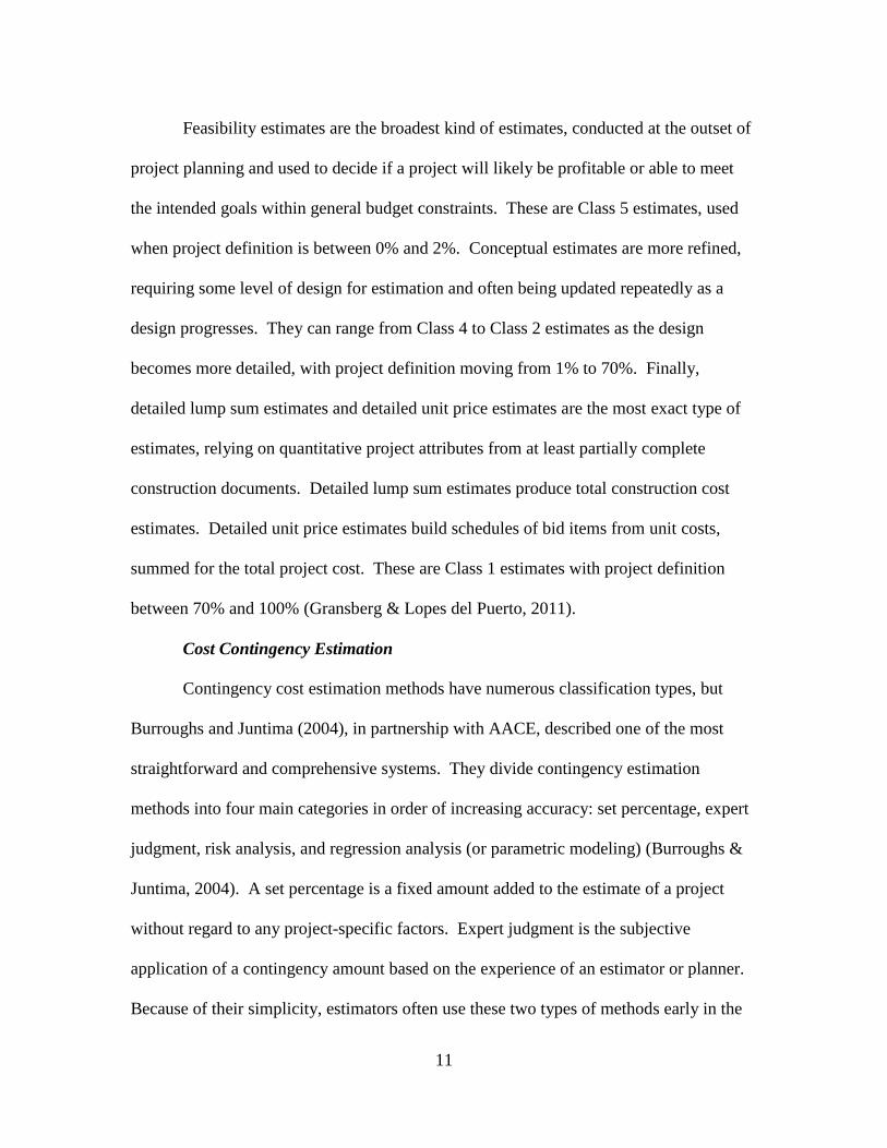
Feasibility estimates are the broadest kind of estimates, conducted at the outset of
project planning and used to decide if a project will likely be profitable or able to meet
the intended goals within general budget constraints. These are Class 5 estimates, used
when project definition is between 0% and 2%. Conceptual estimates are more refined,
requiring some level of design for estimation and often being updated repeatedly as a
design progresses. They can range from Class 4 to Class 2 estimates as the design
becomes more detailed, with project definition moving from 1% to 70%. Finally,
detailed lump sum estimates and detailed unit price estimates are the most exact type of
estimates, relying on quantitative project attributes from at least partially complete
construction documents. Detailed lump sum estimates produce total construction cost
estimates. Detailed unit price estimates build schedules of bid items from unit costs,
summed for the total project cost. These are Class 1 estimates with project definition
between 70% and 100% (Gransberg & Lopes del Puerto, 2011).
Cost Contingency Estimation
Contingency cost estimation methods have numerous classification types, but
Burroughs and Juntima (2004), in partnership with AACE, described one of the most
straightforward and comprehensive systems. They divide contingency estimation
methods into four main categories in order of increasing accuracy: set percentage, expert
judgment, risk analysis, and regression analysis (or parametric modeling) (Burroughs &
Juntima, 2004). A set percentage is a fixed amount added to the estimate of a project
without regard to any project-specific factors. Expert judgment is the subjective
application of a contingency amount based on the experience of an estimator or planner.
Because of their simplicity, estimators often use these two types of methods early in the

12
planning stages of a project when little information is required. However, they also tend
to be the least accurate of the contingency estimation categories (Hollmann, 2008).
Therefore, research has focused on the latter two categories, producing refined methods
for increasing accuracy through risk analysis and regression analysis.
Risk Analysis
Risk analysis can use simulations, such as Monte Carlo, or more deterministic
calculations to produce a confidence interval for a cost estimate. This analysis has
typically relied on a planning team to identify risk or cost distributions subjectively and
input them as parameters in the model. A simulation or algorithm then uses the input
distributions to generate an overall risk or cost distribution for the project as a whole.
One of the more complex examples is the Advanced Programmatic Risk Analysis and
Management (APRAM) method, further refined by in the Modified APRAM method.
These methods take the difference of the expected project cost and the maximum desired
project cost and allocate those funds to specific project activities to buy down risk
through a nonlinear optimization algorithm, minimizing the risk of failure for the project
as a whole (Imbeah & Guikema, 2009; Zeynalian, Trigunarsyah, & Ronagh, 2013).
Slightly less complex is the Estimating using Risk Analysis method, which calculates a
project’s expected and worst-case cost estimate using average and maximum risk
estimates based on expert opinion for each possible project risk (Mak, Wong, & Picken,
1998). Monte Carlo simulations are also used for risk analysis and will be described in
more detail later. Risk Analysis methods typically address project-specific risks
effectively because of the detailed input required for each project (Hollmann, 2008).
However, they also usually require time-consuming efforts and can neglect systemic risks

13
and dependencies between individual distributions because of the model’s complexity
(Burroughs & Juntima, 2004).
Regression Analysis
Regression Analysis is typically described as the most empirical method, relying
on historical cost data trends to estimate the contingency funds required for a current
project (Hollmann, 2008). Using regression analysis, Cook (2006) developed a method
for estimating the contingency funds required for Air Force construction projects,
creating a model using ten factors to predict contingency costs. Another example of this
approach is the regression model developed by Sonmez et al. (2007), which used four
project factors, including the type of contract and a country risk factor derived from
historical data, to estimate contingency costs. They developed this method as a
quantitative model with improved accuracy over expert judgment and with simpler
application compared to complex models such as Monte Carlo simulations. Regression
models, once developed, are often simple to understand and use. This characteristic,
combined with the ability to better address systemic risks than other methods, makes
regression analysis one of the more common cost estimation techniques in use, even
though it does not capture project-specific risks (Hollmann, 2008).
Summary
Across all methods, construction cost estimation theory consistently reinforces the
necessity of identifying the uncertainty inherent in an estimate (Christensen & Dysert,
2011; Hollmann, 2008). The methods available towards this end are then a function of
the level of project definition and the resources available to conduct the estimation.
14
Current State of Air Force Construction Cost Estimation
The Air Force relies on the UFC for recommended cost estimation practices. The
UFC program, developed in response to the House Conference Report 105-247 (1997),
created standardized criteria integrated across the Department of Defense for use in initial
facility planning through construction and maintenance. The Air Force Civil Engineer
Center, United States Army Corps of Engineers, and Naval Facilities Engineering
Command (together called the “Tri-Services”) jointly manage the UFC program
(Department of Defense Standard Practice, 2006).
Unified Facilities Criteria Cost Estimation Methods
For standardized cost estimation methods within the UFC, the tri-services
developed specific techniques derived from the cost estimation categories and practices
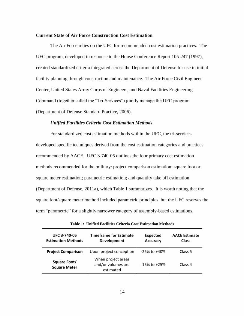
recommended by AACE. UFC 3-740-05 outlines the four primary cost estimation
methods recommended for the military: project comparison estimation; square foot or
square meter estimation; parametric estimation; and quantity take off estimation
(Department of Defense, 2011a), which Table 1 summarizes. It is worth noting that the
square foot/square meter method included parametric principles, but the UFC reserves the
term “parametric” for a slightly narrower category of assembly-based estimations.
Table 1: Unified Facilities Criteria Cost Estimation Methods
UFC 3-740-05 Estimation Methods
Timeframe for Estimate Development
Expected Accuracy
AACE Estimate Class
Project Comparison Upon project conception -25% to +40% Class 5
Square Foot/ Square Meter
When project areas and/or volumes are
estimated -15% to +25% Class 4

15
Parametric When design is 10-30%
complete -10% to +15% Class 3
Quantity Take-Off When design is over 35%
complete -7.5% to +10% Class 2 or 1
AACE associates cost indexes with the various estimation classes (as seen in
Figure 1), which the following sections compared to the UFC 3-740-05’s accuracy range.
An organization can match AACE’s cost index of 1 to the expected accuracy range of
their own final Class 1 estimate, and derive the expected accuracy of earlier class
estimates for the project. The index system provides increased fidelity in the estimation
process by narrowing or widening the accuracy ranges based an organization’s average
accuracy in their final cost estimates. As an example, if an organization expected the
actual project cost to be within 10% of the final estimate, 10% would be associated with
an index of 1. An earlier class of estimate with an index of 5 would then have an
expected accuracy range of within 50%. UFC 3-740-05 states a quantity take-off Class 1
estimate will have a range of -7.5% to +10% within which the actual project costs should
fall (Department of Defense, 2011a). Therefore, for the purpose of this research, an
index of 1 has an expected accuracy range of -7.5% to +10%.
Project Comparison Method
Project comparison cost estimation provides a rough order-of-magnitude cost
during the initial stages of a project’s development when the scope of the project is still
ill-defined (Department of Defense, 2011a). For this method, an estimator compares the
project in question to one or more similar projects accomplished in the past, preferably in
similar environments. The more similar the environment and the more recent the
completion of a comparison project, the more applicable the comparison. The final cost

16
of the comparison project is then scaled to account for differences in scope between the
comparison project and the current project. This scaling is based on a primary measure
of the new project’s capacity such as the number of people or vehicles supported by the
facility or the number of classrooms or uniform room type within the facility. UFC 3-
740-05 notes that the project comparison method provides an estimate with a typical
accuracy of -25% to +40% within which the actual final costs should fall, barring
significant market upheavals or rare and extreme events (Department of Defense, 2011a).
This method falls under the Class 5 cost estimate category of the AACE. Class 5
estimates include expert judgment and basic stochastic methods for use when a project
has 0% to 2% of the project defined (Christensen & Dysert, 2011). A Class 5 estimate
has an expected cost accuracy index of 4 to 20 compared to a completely defined Class 1
estimate with an index of 1 (Christensen & Dysert, 2011). Therefore, this Class 5 project
comparison cost estimate could have an accuracy ranging as narrow as -30% to +40% at
an index of 4 to as broad as -100% to +200% at an index of 20. Because the project
comparison method does not rely only on an estimator’s judgment but also uses some
historical data, the Department of Defense expects the comparison estimates to be on the
optimistic side of the spectrum for Class 5 estimates (Department of Defense, 2011a).
Square Foot or Square Meter Method
The square foot/square meter cost estimate is the next step in the
UFC-recommended estimation process to improve accuracy (Department of Defense,
2011a). For this method, the project scope must be defined enough to include estimated
areas or volumes of the spaces within the proposed facility. Then, using historical data
from a database such as RSMeans, UFC 3-701-01, or the Parametric Cost Engineering
17
System (PACES), a baseline cost can be estimated using per-area or per-volume average
prices. UFC 3-701-01 and PACES rely on data collected in the DoD Tri-Services
Automated Cost Engineering System (TRACES) Cost Book (Department of Defense,
2015). The cost book is, in turn, developed from project records entered into the
Historical Analysis Generator - Second Generation (HII) program, developed by the
United States Army Corps of Engineers (USACE). USACE personnel input all of their
projects into the HII program with the exception of horizontal projects (such as roads)
and facility sustainment, restoration and modernization (FSRM), which are optional
(USACE, 2015). USACE has mandated the addition of project data into the HII
program, or its software predecessor, since 1999 resulting in a relatively comprehensive
database (USACE, 1999).
Once an estimator develops a baseline cost estimate, he or she can then modify
that cost by adjusting for location, project size, price escalation, and other specific
parameters by applying factors often available within the same resources as the historical
databases. Increasing project definition allows for more project-specific adjustments,
which increase the estimate’s accuracy, but the overall accuracy of the square foot/square
meter method typically lies within -15% to +25% (Department of Defense, 2011a).
The square foot/square meter method falls in the Class 4 cost estimate category of
the AACE classification system. Class 4 estimates include stochastic methods using
factors typically for the purpose of a feasibility study (Christensen & Dysert, 2011).
Class 4 estimates are designed for use when a project is between 1% and 15% defined,
with a resulting cost accuracy index of 3 to 12 (Christensen & Dysert, 2011). For the
square foot/square meter method, the accuracy index suggests an accuracy range as
18
narrow as -22.5% to +30% at an index of 3 to as broad as -90% to +120% at an index of
12. As with the project comparison method, UFC 3-740-05 states the expectation the
square foot/square meter method should result in estimates slightly more accurate than a
typical Class 4 estimate (Department of Defense, 2011a).
Parametric Method
Parametric cost estimation, as described in UFC 3-740-05, is an intermediate
estimate recommended when a design is between 10% and 30% complete (Department of
Defense, 2011a). The parametric method uses historical data to estimate the cost of
assemblies and systems within a facility, summing the subtotals for an overall project
estimate. This method provides more accuracy than project comparison or area cost
factors, but with less project definition required for a line item by line item cost estimate
(Department of Defense, 2011a). Parametric cost estimates are expected to have an
accuracy of -10% to +15% (Department of Defense, 2011a).
Within the Air Force, the primary means of accomplishing a parametric cost
estimate is through the software program PACES (Meyer & Burns, 1999). Developed in
the 1980s, PACES uses historical construction costs from the HII database mentioned
earlier. PACES breaks costs down into Work Breakdown Structure line items and
organizes them into the Construction Specifications Institute’s (CSI) MasterFormat
structure as detailed in the PACES 2005 Training Manual for the Air Force (Earth Tech,
2005). PACES includes a range of cost estimates from an initial area cost factor Class 4
estimate as mentioned in the square foot/square meter method section, to a relatively
detailed Class 2 estimate. An estimator can start with default project parameters for an

19
initial estimate and add information to improve the estimate’s accuracy as a project
becomes more defined (Earth Tech, 2005).
The parametric method primarily produces Class 3 estimates. An estimator
develops these estimates for projects with 10% to 40% of the design complete and can
provide enough fidelity for budget projections (Christensen & Dysert, 2011). Class 3
estimates should have a cost accuracy index from 2 to 6 (Christensen & Dysert, 2011),
indicating an accuracy range of -15% to +20% at an index of 2 and -45% to +90% at an
index of 6 for Air Force Class 3 estimates in general. However, the Department of
Defense expects the parametric method, in particular, to be more accurate than the typical
Class 3 range, with the previously mentioned accuracy range of -10% to +15%
(Department of Defense, 2011a).
Quantity Take-Off Method
The final and most accurate method for cost estimation recommended by UFC 3-
740-05 is the quantity take-off method (Department of Defense, 2011a). Estimators
using this method divide a project into as many, individually priced, specific work
increments as is feasible. With their associated quantities and unit costs, these
increments subtotal and sum together into an overall project cost estimate. Typically a
35% design, at a minimum, is required to supply the level of detail need for this type of
estimate, and the expected accuracy is -7.5% to +10% (Department of Defense, 2011a).
The quantity take-off method can be considered either a Class 2 or Class 1
estimate depending on how well defined the project is. Class 2 estimates typically
require a project to be 30% to 70% defined whereas Class 1 estimates require 70% to
100% of a project to be defined (Christensen & Dysert, 2011). A Class 1 estimate
20
provides the baseline for the expected accuracy range of earlier estimates with an index
of 1 (Christensen & Dysert, 2011). Therefore, the quantity take-off method’s expected
accuracy of -7.5% to +10% was used in this paper as a baseline to compare the expected
accuracies of earlier stage estimates outlined in UFC 5-740-05 with the accuracy index
range expected by AACE.
Summary
None of the methods currently recommended for use in Air Force construction
cost estimation include a simulation analysis method. Furthermore, Air Force research
has focused primarily on factor analysis and parametric models to improve cost
estimates. Several Air Force research efforts have analyzed factors impacting a project’s
schedule performance, overall project success, and the number of project change orders
in Air Force construction (Beach, 2008; Hoff, 2015; Nielsen, 2007). Two studies
developed parametric models for estimating project costs. One study predicted
contingency fund requirements for Air Force MILCON projects using historical data
trends (Cook, 2006) and the second used expert opinion to model impacts of several
factors on Air Force project costs in general (Stark, 1986). Appendix A summarizes
other similar Air Force construction cost research.
The lack of a simulation method, both in practice and as a focus of research, is of
interest because simulations are recommended by the Government Accountability Office
(2009) for increased accuracy in cost estimation in the Air Force (Air Force Cost
Analysis Agency, 2007). Specifically, the Government Accountability Office (2009)
explicitly states that using a simulation to estimate cost is better than the summation of
the most likely element costs, which is usually inaccurate. Step 9 of their “Twelve Steps
21
of a High-Quality Cost Estimation Process” involves using simulation to conduct
uncertainty analysis for a given point estimate (U.S. Government Accountability Office,
2009). The Air Force Cost Analysis Agency (2009) provides three methods of analyzing
uncertainty in a cost estimate, two of which are simulation-based. The third option, the
scenario-based method, is only recommended when there are not enough resources or
data to support one of the simulation-based methods (Air Force Cost Analysis Agency,
2007). Therefore, a construction-specific simulation method adapted from industry
research could bring significant insight into expected project costs after the initial, highly
uncertain factor analysis estimates and before the parametric cost estimate developed
during design. Decision makers would then have access to a more accurate cost estimate
during the budget and approval process before design commencement.
The Monte Carlo Method
The Monte Carlo method was developed by Stan Ulam and John von Neumann in
the 1940s to estimate the results of combining a complex set of uncertainties together
when the direct calculation of the final probabilities would be intractable (Metropolis &
Ulam, 1949). Initially used for modeling atomic reactions at Los Alamos in the
development of thermonuclear and fission devices (Eckhardt, 1987), the technique is
ideal for the combination of cost distributions, resulting in a significantly more reliable
estimate than just summing the averages of each subordinate distribution (Savage, 2012).
However, the method requires careful modeling to cover systemic risks and dependencies
between distributions. Therefore, the following sections provide an overview of the
development of the model for construction cost estimate along with a review of
techniques for compensating for some of the model’s limitations.
22
Development for Construction Applications
Initially, available computer computational ability limited the use of Monte Carlo
simulations for construction cost and schedule estimates. A study in 1991 highlighted
this fact with the development of a computer program that took activity range inputs and
calculated the overall cost and time for the project using a Monte Carlo simulation
(Willmer, 1991). The program had to be broken up into parts and run separately because
the available computers could not run the whole simulation at once. Further
advancements in technology minimized the computational restrictions and more useful
and realistic models were developed using Monte Carlo simulations, such as Dawood and
Nashwan’s Monte Carlo Network Analysis (1998) and the Judgmental Risk Analysis
Process (Öztaş & Ökmen, 2005). Both of these models estimate project duration using
risk probability distributions. The technique advanced in the cost arena as well, resulting
in construction organizations beginning to rely on Monte Carlo analysis for detailed cost
estimation (Clark, 2001).
Monte Carlo Improvements
Despite widespread use, many research studies and organizations have not applied
systemic risk factors or correlations between items in their Monte Carlo estimates,
including the studies previously mentioned. Ignoring systemic risk factors, such as
project location, in a line-item based simulation removes potentially significant effects on
the project as a whole, reducing the model’s accuracy and utility (Hollmann, 2007).
Instead of ignoring these systemic risk factors, parametric models can adjust the Monte
Carlo simulation results for systemic risk factors.

23
However, parametric modeling adjustments to a Monte Carlo simulation only
address whole-project risk affects, while potential inaccuracies remain within the model
without appropriate correlations. For example, electrical and mechanical costs tend to
rise and fall together, but if estimators fail to include this relationship, additional error is
introduced into the estimate (Chau, 1995a). Chau (1995a) went on to investigate the
effects of using different types of distributions to model construction cost data,
concluding that triangle distributions tended to introduce unnecessary error and instead
beta and lognormal distributions were preferred. Wall’s (1997) research further analyzed
distribution types for cost data and recommended the lognormal distribution over the beta
distribution when modeling historical data. The types of distributions chosen play a key
role in correlation modeling because the most common type of correlation, the Pearson’s
correlation, typically relies on normal distributions to correlate. Since historical cost data
does not often fit a normal distribution, a transformation to normal distributions would
likely be required. Alternatively, Spearman or rank correlations provide an avenue to
correlate distributions of any type without transformation and were shown to be viable in
Monte Carlo cost estimates (Touran & Suphot, 1997). With accurate distribution
modeling, appropriate correlations, and systemic risk factors accounted for, a Monte
Carlo simulation can overcome many of the otherwise inherent disadvantages.
Conclusion
Point estimates for cost do not provide insight into a project’s uncertainty and the
resulting risk to the organizations involved because a single point hides the range within
which the cost could fluctuate. Summations of expected values often do not take into
account correlations between project items, resulting in unintentionally skewed estimates
24
due to unaccounted internal interdependencies. However, the Air Force has focused
construction cost estimation research, along with recommended estimation methods, on
parametric models and general factor analysis. These models produce a point estimate
after providing adjustments to a single project expected value or a summation of project
element expected values. While the resulting estimates are useful, the Air Force could
benefit from a method that provides additional insight into an estimate’s uncertainty and
can model project risks more accurately while still being executable before the design
phase of a project. A Monte Carlo simulation may be able to provide those benefits,
assisting decision makers at the time Air Force projects are budgeted and approved and
before significant errors in an estimate cause program upheavals to correct.

25
III. Methodology
Chapter Overview
The purpose of this research is to develop a cost-estimating tool that can provide a
more accurate estimate than current practices using a basic 15% design. This
methodology chapter describes the steps used to develop the model. The model used a
Monte Carlo simulation to estimate individual project costs based on historical data. The
first section provides an overview of the Monte Carlo method and the specific application
used in the model. The second section describes the data collection effort. The third
section describes the steps used to develop representative distributions to model
individual cost elements along with correlations between those cost elements. Finally,
the fourth section describes the model validation.
Monte Carlo Simulation
Element distributions and correlation matrices between those elements form the
foundation of the Monte Carlo simulation used in this research. In general, the
simulation takes a random sample from each element distribution, correlates them
according to the correlation matrix, and outputs the results as one trial. This process
repeats numerous times. The Monte Carlo simulation collects data from each trial,
adding them to a histogram showing the various results. After over tens of thousands of
simulation trials, the histogram becomes stable, revealing the probability of specific
results based on their frequency in the histogram. To build this type of Monte Carlo
simulation, Iman and Conover developed a method for correlating multivariate random
variables, such as those studied here, with a rank correlation matrix (1982). Their

26
method allows for the use of any input distribution without concern for normality,
including the use of distinct types of input distributions simultaneously for different
variables. Additionally, this technique preserves the integrity of the sampling method
used, allowing methods such as the Latin Hypercube Sampling, described later, without
distorting the intervals. Finally, their method also provided better results for producing
outputs more closely following the given correlation relationships compared to other
random sampling techniques (Iman & Conover, 1982). Other studies have used Iman and
Conover’s method to simulate correlated construction cost, further validating the
method’s utility for this research (Touran & Suphot, 1997). Given their method, also
available in software packages for programs including the R Project for Statistical
Computing, the researcher established a Monte Carlo simulation model.
Within the simulation model, the nature of the sampling method affects the
results. Simple random sampling is the most basic sampling method, drawing numbers
using a computerized random-sampling algorithm from within the distribution
parameters. Latin Hypercube Sampling is an alternate option, dividing a given
distribution into equal-probability intervals and drawing a proportional number of
samples from each interval (Air Force Cost Analysis Agency, 2007). Latin Hypercube
Sampling preserves the overall proportions of the distribution being sampled, reducing
concerns of bias introduced randomly through the simple sampling process. Increasing
the number of samples taken minimizes the likelihood of a random bias from simple
random sampling, but Latin Hypercube Sampling minimizes such a bias from the outset
while allowing the simulation to converge to the true mean with fewer iterations. Several
government agencies also recommends Latin Hypercube Sampling for government cost
27
estimation (Air Force Cost Analysis Agency, 2007; U.S. Government Accountability
Office, 2009). Therefore, for this study, each simulation ran 100,000 trials through a
Latin Hypercube Sampling method to estimate complete and accurate distributions for
the final analysis.
The simulation outputs 100,000 sample costs for each of the cost elements
identified. As a result, each of the 100,000 rows, comprising of one each of the 11 cost
elements correlated together, is a generic cost summary per unit for the given facility
type. The summation of each row provides a cost estimate total. Taking each of these
100,000 sample cost summaries, the model developed here created a cost distribution
histogram for each facility type studied. These costs, multiplied by the desired facility
scope and adjusted for the desired construction date and location, produce a project-
specific cost estimate. If desired, the cost elements may remain separate throughout these
calculations, providing a review of the element costs within the total cost, or summed
together for the overall cost estimate.
Data Collection
The Department of Defense stores Air Force historical construction project data in
several different databases. The Air Force has the most comprehensive database in the
Automated Civil Engineer System (ACES). Both the United States Army Corps of
Engineers (USACE) and the Naval Facilities Engineering Command (NAVFAC) also
have project data for military construction (MILCON) projects they execute for the Air
Force. While the Air Force maintains general information on every construction project
type within ACES, each engineering squadron or agency records much of the specific
project details locally and not in a central repository for simple retrieval. Data quality is
28
also an issue, with many of the information fields in ACES for a given project remaining
blank or containing errors. USACE has more detailed records in their databases,
specifically in the Resident Management System (RMS), but access to the system is
limited to approved individuals with RMS-specific software. Therefore, the researcher
examined both ACES and RMS as possible data sources to obtain project costs. The
criteria for acceptable data included completed Air Force construction projects with
detailed cost line items useful in identifying the subtotal costs of the main cost elements
within each project. This research also required information on the scope of each project,
convertible to either square feet or square meters, along with the location, facility type,
and mid-point date of construction. With these components, the rest of the analysis could
commence.
Cost Element Selection
Selecting appropriate cost elements to describe the main components of a
project’s overall cost set the foundation for the rest of the methodology. Past research
has limited the number of cost elements to analyze within a project to between 5 and 15
(Touran & Suphot, 1997; Touran & Wiser, 1992; Wall, 1997; Yang, 2005). Using every
detailed cost line item would be impractical, creating significant issues defining
distributions and associated correlations that accurately describe the majority of the
projects in a set. Instead, Touran and Wiser suggest that the items on a cost summary
sheet provide a sufficient level of detail (1992, p. 259). Humphreys’ assertion supports
this concept that less than 20 cost items in a given construction estimate are critical items.
They contribute to a majority of the cost risk, with those 20 or fewer items being the only
items significant enough to change the cost by more than 0.5% if their inherent risk is
29
realized (Humphreys, 2008). Therefore, defining a large number of cost elements for
analysis is unnecessary if only a small portion will indeed alter the overall cost
significantly. To build on these lessons, the researcher sought to define between 5 and 15
cost elements of a similar type to those used in past research and which followed the
general format of the CSI MasterFormat divisions. The military relies on the CSI
MasterFormat divisions as a primary means of categorizing costs during the estimation
process (Earth Tech, 2005), providing an initial framework for the cost elements in this
study.
Construction costs, particularly individual line item costs, can come in many
forms particular to the contractor supplying them, requiring a method to transform varied
estimate into summaries fitting within the cost elements chosen as described earlier.
Such a method was especially necessary when using data from the RMS database
managed by USACE. RMS records each cost line item billed by a construction
contractor to the government. For large MILCON projects, such as is the focus of this
study, those line items can number in the thousands. Additionally, the line item
description consists of any phrase or code the contractor deemed useful for bookkeeping
and for which the government Contracting Officer accepted. There are no enforced
standard or wording criteria for what is considered a minor record of cost identifiers
useful only infrequently in the administration of a contract. Furthermore, when
contractors or government personnel summarize these line items, they group them either
into one aggregate cost for the entire project or by major contract line item number
(CLIN). CLINs describe major components of the product desired by function, not
construction effort or specialties. Therefore, to categorize the many thousands of
30
dissimilar line items into meaningful cost elements, the researcher built a list of
keywords, phrases, acronyms, and abbreviations associated with each cost element.
Then, a search function could scan the line item descriptions for the keywords and
categorize the costs appropriately. This search also required an order of precedence for
the keywords for situations when a single line item contained multiple keywords,
resulting in the correct categorization of that item. Appendix C lists the keywords,
phrases, and abbreviations in the order of precedence used. The abbreviations include
truncated words and intentional mis-spellings to account for the shorthand used by many
contractors.
In addition to having line items categorized into cost elements that adequately and
succinctly describe the overall project costs, those cost elements also needed to be
standardized based on a common unit of measure and based on systemic factors (Yang,
2005, p. 279). The common unit of measure is typically square feet or square meters and
is necessary to compare and correlate the elements with each other as well as to compare
items between projects of different scope (Yang, 2005). Standardizing based on systemic
factors removes cost differences based on location or timeframe and yields a more
accurate representation of general construction costs (Yang, 2005, p. 279). this study, the
model used the UFC 3-701-01 DoD Facility Pricing Guide’s area cost factors and
escalations factors to standardize the cost data with a generic location index of 1 and
based in October 2014 dollars (2015).
Another key systemic factor affecting project cost is the facility type. Different
types of facilities drive variations in cost due to the differences in construction efforts
required. Therefore, the model focuses on simulating costs based on facility type. Past

31
research has predominantly focused on similar office buildings as a source of uniform
data to analyze (Touran & Suphot, 1997; Touran & Wiser, 1992; Wall, 1997; Yang,
2005). The Air Force builds a much wider variety of facilities to support its mission than
simply office buildings. Therefore, this research focused initially on airfield and airfield-
related projects, sorting projects by category code (CATCODE) into groupings similar to
the UFC 3-701-01 DoD Facility Pricing Guide (2015). However, due to the limited
amount of airfield-specific projects and other facility types available in the data, the
researcher could only analyze dormitories, education and training facilities, and squadron
operations facilities. The model then took each facility-type grouping and applied the
rest of the following methodology, resulting in a cost estimate profile specific to each
facility type.
Distribution Characterization
Each cost element needed a distribution describing the element’s behavior for
modeling. Triangular distributions have historical precedence in modeling construction
costs because of their direct application to subject matter expert’s estimates. However,
Chau argues that either generalized beta or lognormal distributions are a better fit for
historical data (1995b). Additionally, other authors have suggested that the lognormal
distribution is a better fit for historical construction cost data than the generalized beta
(Touran & Wiser, 1992; Wall, 1997). Table 2 shows a sampling of past research
detailing the construction cost elements past authors selected and the distributions they
associated with those elements. Additionally, these authors correlated the elements
shown in clear cells in Table 2 with the rest in their model. Touran concedes that the
unbounded positive tail of the lognormal may need to be truncated in some cases, but this

32
is typically not necessary due to the extremely remote probabilities represented by the
parts of the tail that could produce an unreasonable cost sample (1993, p. 69).
Table 2: Cost Element Selection and Associated Distributions from Past Research
Touran & Wiser (1992) Touran & Suphot (1997) Yang (2005)
Elements Dist Elements Distribution Elements Distribution
General & Overhead
Lo
gn
orm
al (all elemen
ts)
Sitework Gamma Substructure Lognormal
Site Work Concrete Lognormal Superstructure Lognormal
Concrete Masonry Gamma Internal Finishes Lognormal
Masonry Metals Beta Fittings & Discrete
Metals Carpentry
Beta/Log- Furnishings
Carpentry normal Services Beta
Moisture Protection Moisture Lognormal
External Works Beta
Doors, Windows, Glass Protection Preliminaries Lognormal
Finishes Doors, Windows, Lognormal
Contingencies Lognormal
Specialties Glass
Equipment Finishes Gamma
Furnishings Mechanical Gamma
Conveying Systems Electrical Erlang
Mechanical
Electrical
Elements not correlated with the others in the specified model
To identifying distribution candidates for each cost element, the researcher plotted
the cost element data sets on a Cullen and Frey graph. The Cullen and Frey graph plots
the data’s estimated square of skewness (x-axis) versus kurtosis (y-axis) with common
distributions shown as points, lines, or shaded regions, depending on the parameters of
that particular distribution (Delignette-Muller & Dutang, 2014). For example, the normal
distribution has only one skewness and kurtosis location on the graph, shown as a single
point. Alternatively, the graph shows lognormal and gamma distributions as a line due to
their potential variation in skewness and kurtosis, whereas the beta distribution is a region
because of the four parameters defining a much wider variety of possible shapes
33
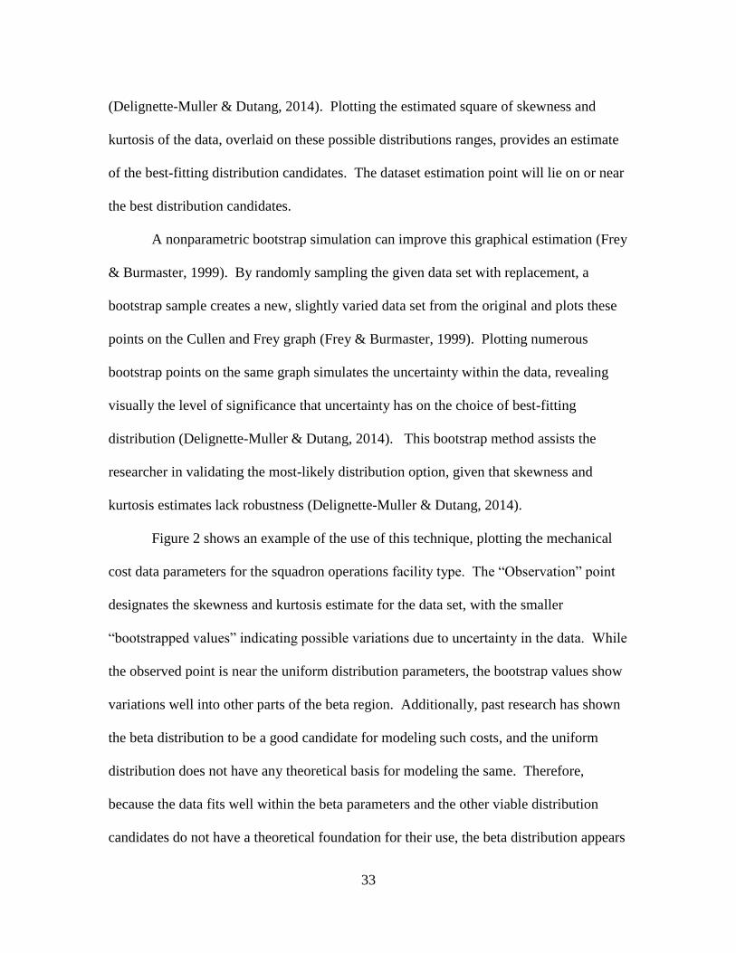
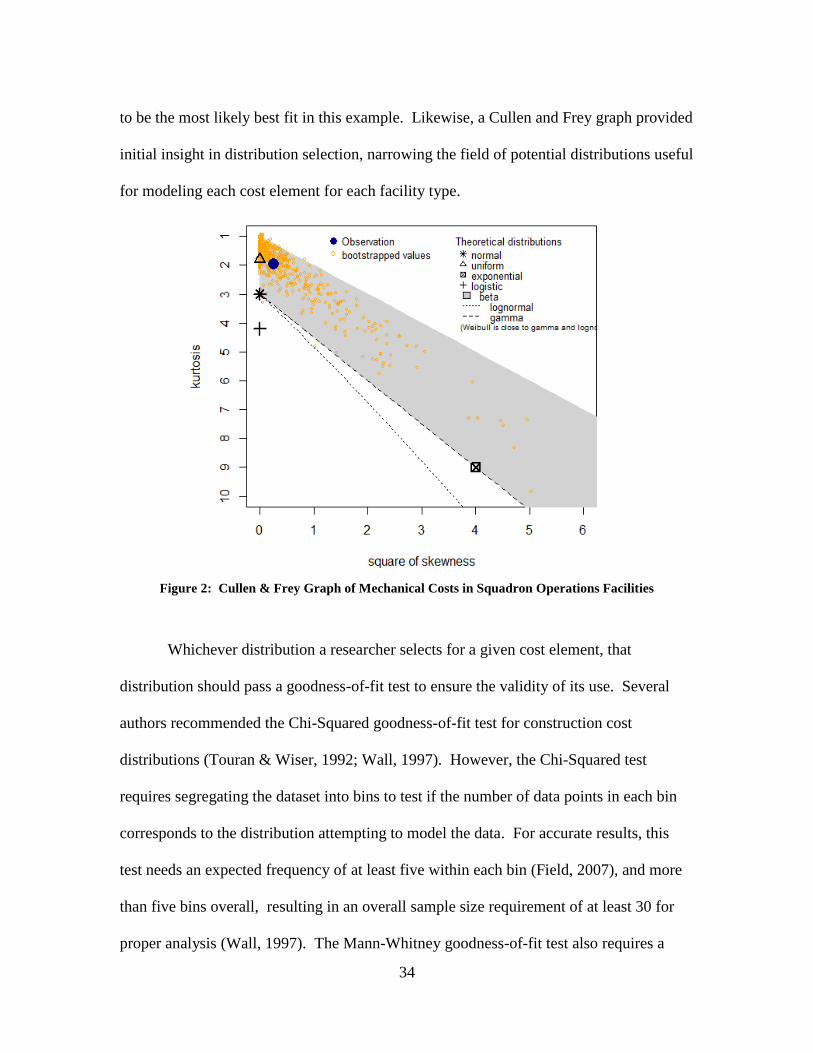
(Delignette-Muller & Dutang, 2014). Plotting the estimated square of skewness and
kurtosis of the data, overlaid on these possible distributions ranges, provides an estimate
of the best-fitting distribution candidates. The dataset estimation point will lie on or near
the best distribution candidates.
A nonparametric bootstrap simulation can improve this graphical estimation (Frey
& Burmaster, 1999). By randomly sampling the given data set with replacement, a
bootstrap sample creates a new, slightly varied data set from the original and plots these
points on the Cullen and Frey graph (Frey & Burmaster, 1999). Plotting numerous
bootstrap points on the same graph simulates the uncertainty within the data, revealing
visually the level of significance that uncertainty has on the choice of best-fitting
distribution (Delignette-Muller & Dutang, 2014). This bootstrap method assists the
researcher in validating the most-likely distribution option, given that skewness and
kurtosis estimates lack robustness (Delignette-Muller & Dutang, 2014).
Figure 2 shows an example of the use of this technique, plotting the mechanical
cost data parameters for the squadron operations facility type. The “Observation” point
designates the skewness and kurtosis estimate for the data set, with the smaller
“bootstrapped values” indicating possible variations due to uncertainty in the data. While
the observed point is near the uniform distribution parameters, the bootstrap values show
variations well into other parts of the beta region. Additionally, past research has shown
the beta distribution to be a good candidate for modeling such costs, and the uniform
distribution does not have any theoretical basis for modeling the same. Therefore,
because the data fits well within the beta parameters and the other viable distribution
candidates do not have a theoretical foundation for their use, the beta distribution appears
34
to be the most likely best fit in this example. Likewise, a Cullen and Frey graph provided
initial insight in distribution selection, narrowing the field of potential distributions useful
for modeling each cost element for each facility type.
Figure 2: Cullen & Frey Graph of Mechanical Costs in Squadron Operations Facilities
Whichever distribution a researcher selects for a given cost element, that
distribution should pass a goodness-of-fit test to ensure the validity of its use. Several
authors recommended the Chi-Squared goodness-of-fit test for construction cost
distributions (Touran & Wiser, 1992; Wall, 1997). However, the Chi-Squared test
requires segregating the dataset into bins to test if the number of data points in each bin
corresponds to the distribution attempting to model the data. For accurate results, this
test needs an expected frequency of at least five within each bin (Field, 2007), and more
than five bins overall, resulting in an overall sample size requirement of at least 30 for
proper analysis (Wall, 1997). The Mann-Whitney goodness-of-fit test also requires a

35
sample size of at least 25, while the Kolmogorov-Smirnov goodness-of-fit test is viable
despite small sample sizes (Field, 2007). Because the data available in this research
consisted of small sample sizes (between 8 and 20), the Kolmogorov-Smirnov goodness-
of-fit test proved the most viable method to measure the hypothesis that a given
distribution could accurately model a given cost element.
Correlation Characterization
As established in Chapter II of this research, defining accurate correlations
between the cost elements is a critical step in developing a complete cost model. A
common measure of correlation is the Pearson’s correlation, or product-moment
correlation, but this measure assumes a linear relationship between normally distributed
samples (Yang, 2005). The distributions of the cost elements studied here were not likely
to be normally distributed; therefore requiring a different correlation measure. Kendall’s
tau correlation coefficient provided a non-parametric alternative but is only preferred
over Spearman’s correlation coefficient when the data contains a significant amount of
tied ranks (Field, 2007). As this is typically not the case with continuous cost data,
Spearman’s correlation coefficient proved the most viable correlation method. The
Spearman’s correlation, or rank correlation, uses the relative ranking of the elements
within a sample, and compares the order of the ranking in one variable to the next,
applying a product-moment correlation to the ranks instead of the values themselves
(Yang, 2005). The ranks are the relative position of each element within a variable when
sorted by cost. The formula shown in Equation 1compares the ranks of corresponding
cost elements, defining a correlation coefficient between each element. A correlation
matrix then combines these coefficients for use in simulations.

36
2
1
2
6 (x y )
1( 1)
n
i i
ixyr
n n
(1)
Equation 1: Spearman’s Correlation Coefficient
Where rxy Spearman correlation coefficient between variables X and Y
xi rank of ith
value of variable X
yi rank of ith
value of variable Y
n sample size
After deriving a correlation matrix as described, one more step remains before
integration into the simulation. The correlation matrix must be positive definite for use in
a Monte Carlo simulation (Yang, 2005). This requirement posed a potential issue
because, as Yang notes, the more elements included in a model such as this, the more
likely the correlation matrix will be infeasible (2005, p. 277). Higham provides an
algorithmic solution, developed for a similar application of finding the nearest feasible
correlation matrix from an infeasible matrix correlating stock prices (2002). This
method, available within statistical software for programs such as the R Project for
Statistical Computing, completes the correlation process, creating from an infeasible
matrix a positive definite matrix. Viable distributions for each cost element and feasible
correlation matrices are then both available for simulation.
Validation Process
Model validation required using several projects not part of the model
development on which to test the model for accuracy; five projects were set aside for this
purpose. The validation set included one dormitory project, two education and training
projects, and two squadron operation projects. These quantities correspond to 10%

37
(rounded up) of the collected sample sizes for each facility type. The validation projects
did not factor into the distribution modeling, correlation analysis, or Monte Carlo
simulation so as not to bias the results toward the validation projects. The developed
model then estimated costs for the five reserved projects. For each project, the researcher
multiplied the appropriate facility type distribution developed in the simulation with the
project’s scope and adjusted for the project’s location and midpoint construction date.
The UFC 3-701-01 DoD Facility Pricing Guide (2015) provided the area cost and
timeframe escalation adjustment factors. Comparing this estimate to the actual project
cost revealed the accuracy of the model for each of the five projects. Additionally,
comparing this estimate to the programmed amount (PA) showed the relative accuracy of
this model to the estimate used in the programming phase of the project.
However, cost estimators develop and improve the initial PA during the first
stages of a project’s design, creating a Class 3 parametric cost estimate with a design
level between 10-25% (Department of Defense, 2011a, p. 5, 2011b, p. 6). They then
further refining that estimate with a design level between 35-65% (Department of
Defense, 2011a, p. 11). This process results in a cost estimate more accurately described
as a Class 2 estimate according to AACE, with an expected accuracy of -7.5% to +10%.
The updated PA overwrites the initial PA amount recorded in project databases and
therefore used by this research for comparison. The estimate developed by this research
model relies on only basic scope information, resulting in a Class 4 estimate with an
expected accuracy of -15% to +25%. Therefore, while noteworthy if the model performs
better than the recorded PA, the comparison is not direct. Both the UFC 3-701-01 DoD
Facility Pricing Guide (2015) and the AFCESA Historical Air Force Construction Cost
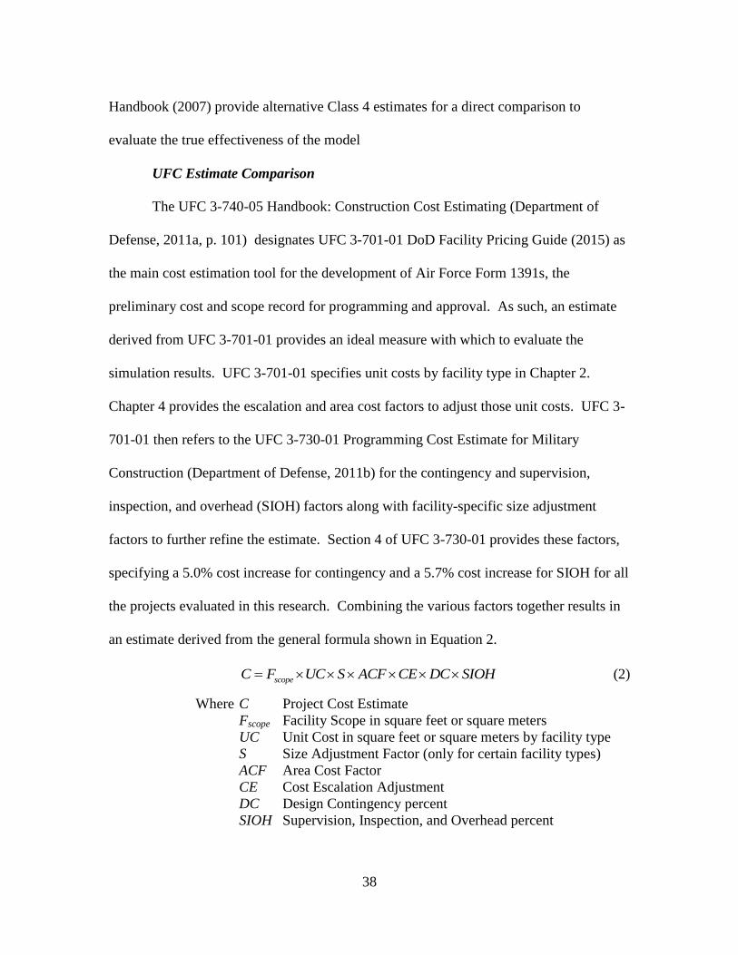
38
Handbook (2007) provide alternative Class 4 estimates for a direct comparison to
evaluate the true effectiveness of the model
UFC Estimate Comparison
The UFC 3-740-05 Handbook: Construction Cost Estimating (Department of
Defense, 2011a, p. 101) designates UFC 3-701-01 DoD Facility Pricing Guide (2015) as
the main cost estimation tool for the development of Air Force Form 1391s, the
preliminary cost and scope record for programming and approval. As such, an estimate
derived from UFC 3-701-01 provides an ideal measure with which to evaluate the
simulation results. UFC 3-701-01 specifies unit costs by facility type in Chapter 2.
Chapter 4 provides the escalation and area cost factors to adjust those unit costs. UFC 3-
701-01 then refers to the UFC 3-730-01 Programming Cost Estimate for Military
Construction (Department of Defense, 2011b) for the contingency and supervision,
inspection, and overhead (SIOH) factors along with facility-specific size adjustment
factors to further refine the estimate. Section 4 of UFC 3-730-01 provides these factors,
specifying a 5.0% cost increase for contingency and a 5.7% cost increase for SIOH for all
the projects evaluated in this research. Combining the various factors together results in
an estimate derived from the general formula shown in Equation 2.
scopeC F UC S ACF CE DC SIOH (2) Equation 2: UFC 3-701-01 Generic Cost Estimation Formula
Where C Project Cost Estimate
Fscope Facility Scope in square feet or square meters
UC Unit Cost in square feet or square meters by facility type
S Size Adjustment Factor (only for certain facility types)
ACF Area Cost Factor
CE Cost Escalation Adjustment
DC Design Contingency percent
SIOH Supervision, Inspection, and Overhead percent

39
AFCESA Estimate Comparison
The AFCESA Cost Handbook (2007) is not as widely used in practice as it is an
older cost estimation guide compared to the 2014 cost data built into UFC 3-701-01 DoD
Facility Pricing Guide (2015). However, similar data collection and methodologies went
into the creation of the handbook compared to UFC 3-701-01. Additionally, the
AFCESA Handbook is specific to Air Force construction whereas UFC 3-701-01 creates
estimates usable by the Army, Navy, and Air Force in general. While the larger scope of
UFC 3-701-01 allowed it to use larger data sets for the development of its models, the
AFCESA Handbook may remove some systematic errors with a more tailored estimate
due to its narrower focus. Therefore, it provides a worthwhile cost estimate comparison
both to measure the simulation model against, as well as to highlight any trends in the
differences between a military-overall estimate from UFC 3-701-01 and an Air Force-
specific estimate from the AFCESA Handbook.
Despite employing different data, the AFCESA Handbook uses similar data tables
and formulas to develop a cost estimate. Section II provides historical data by facility
type, standardized to October 2007 dollars and shown in cost per square feet. AFCESA
removed contingency costs and SIOH from these unit costs as well. Section IV provides
size adjustment tables, Section V provides escalation tables, and Section VI provides
location factors. Finally, Section VIII provides the same contingency amount of 5% and
SOIH amount of 5.7% as UFC 3-701-01. The validation estimates for this study did not
use Section VIIs supporting facility data. Taking these factors and adjustments,
AFCESA uses the same general formula depicted in Equation 2 to develop a cost
estimate.
40
Summary
The general concept of this methodology was to conduct a thorough and detailed
analysis of project cost estimates for a variety of projects. Then, through careful
modeling using the best practices and lessons learned from cost estimation experts,
develop a simple tool for accurate cost estimation in the early stages of a given project.
The facility-type cost distributions output by the Monte Carlo simulation are that tool.
With a general scope, a location, and a construction timeframe, an estimator can apply
the appropriate factors to a distribution, and have not only an expected cost but also an
illuminating range of possible costs and their probabilities. The analysis and results
chapter next assesses if this tool is indeed accurate, meeting the AACE Class 4 standards,
and if it is an improvement or provides any additional insight over the current estimation
methods available.

41
IV. Analysis and Results
Chapter Overview
The Monte Carlo cost estimation model proposed in Chapter III provided cost
estimates better than, or comparable to, the programmed cost estimates in three of the
five measures. Moreover, the simulation provided valuable insight despite being less
accurate for the other two measures by evaluating project-specific circumstances. This
finding is significant because the source data had issues in both quality and quantity.
Data collection and quality assurance became significant challenges, restricting the
number of facility type models this research could have otherwise created and limiting
the ability to validate the models that this research did create. Such performance despite
data issues indicates the potential utility of this methodology in Air Force military
construction (MILCON) or sustainment, restoration, and maintenance (SRM) cost
estimation.
Methodology Implementation
The following sections detail the various steps taken in implementing the
proposed methodology. Microsoft Excel (2010) spreadsheets provided the platform for
data collection, cost element categorization, and cost element standardization. The R
Project for Statistical Computing software provided the platform for distribution
modeling, correlation modeling, simulation modeling, and the final model validation
steps. Appendix E displays the program code used in the R Project software for this
analysis.

42
Data Collection
Data collection in itself proved to be a significant challenge for this research. The
proposed methodology required large samples of similar-type facility projects along with
a detailed line item list of final costs, a measure of scope, and a programmed cost
estimate for each project. The Air Force’s primary facility cost database, ACES, had
substantially more projects than needed but did not track the line item costs of those
projects. ACES only recorded the total cost of projects, with some cases providing costs
broken out by contract line item. Contract line item costs did not provide the detail
required, annotating only the primary deliverables of a project without regard to the
construction specialties or methods used for those deliverables.
The USACE, as the primary MILCON execution agent for the Air Force, has their
own database, namely the Resident Management System (RMS), for tracking projects
given to them by the Air Force. This research focused on MILCON projects. Therefore,
the researcher considered using RMS data. While ACES records primarily high-level
information for MILCON project programming and approval purposes, RMS records
every project and contract document from the bidding process to final close-out. With
the assistance of several RMS database experts from USACE, the researcher obtained a
spreadsheet of all available Air Force MILCON projects in the system. This list included
177 projects from 2001 to 2014 with an average of 370 cost line items each.
However, to use the collected data, each project needed a measure of scope and a
programmed cost estimate with which to compare the final results. Because RMS
primarily tracks project data starting at the bidding phase of project execution, estimates
from the Air Force’s programming phase are not included. Additionally, the RMS data

43
pull did not contain a consistent measure of scope for each project. Therefore, the
researcher matched the projects from the RMS data to the associated ACES projects and
removed projects out of the list that did not have the measures needed for analysis. This
effort required cutting all projects earlier than 2005 because ACES did not keep project
records before this date. Missing data also necessitated the removal of several other
projects.
The proposed methodology required further data trimming in several other areas.
The focus of this research was on Air Force construction within the U.S., necessitating
the removal of all construction projects in foreign countries. Additionally, the projects
had to be grouped together by facility type, and most type categories contained six or
fewer projects, further limiting the sample size. The researcher kept only categories with
eight projects or more. Finally, several projects had data inconsistencies or line items
that combined a majority of the project costs into one single cost unsuitable for analysis.
The researcher eliminated these projects as well. The final data set prepared for analysis
included 43 projects: 20 of which the researcher classified as education and training
facilities, 15 as squadron operation facilities, and 8 as dormitories. Each project had an
average of 400 cost line items.
Cost Element Categorization
To find cost trends, the researcher had to categorize each cost line item within an
overall cost category. The data fit into 11 major categories for each of the three facility
types with a cost summary shown in Table 3. These categories loosely follow major CSI
MasterFormat divisions as indicated, with the main exception of dividing the material
specialty types of concrete, masonry, metals, and wood (CSI MasterFormat Divisions 3,
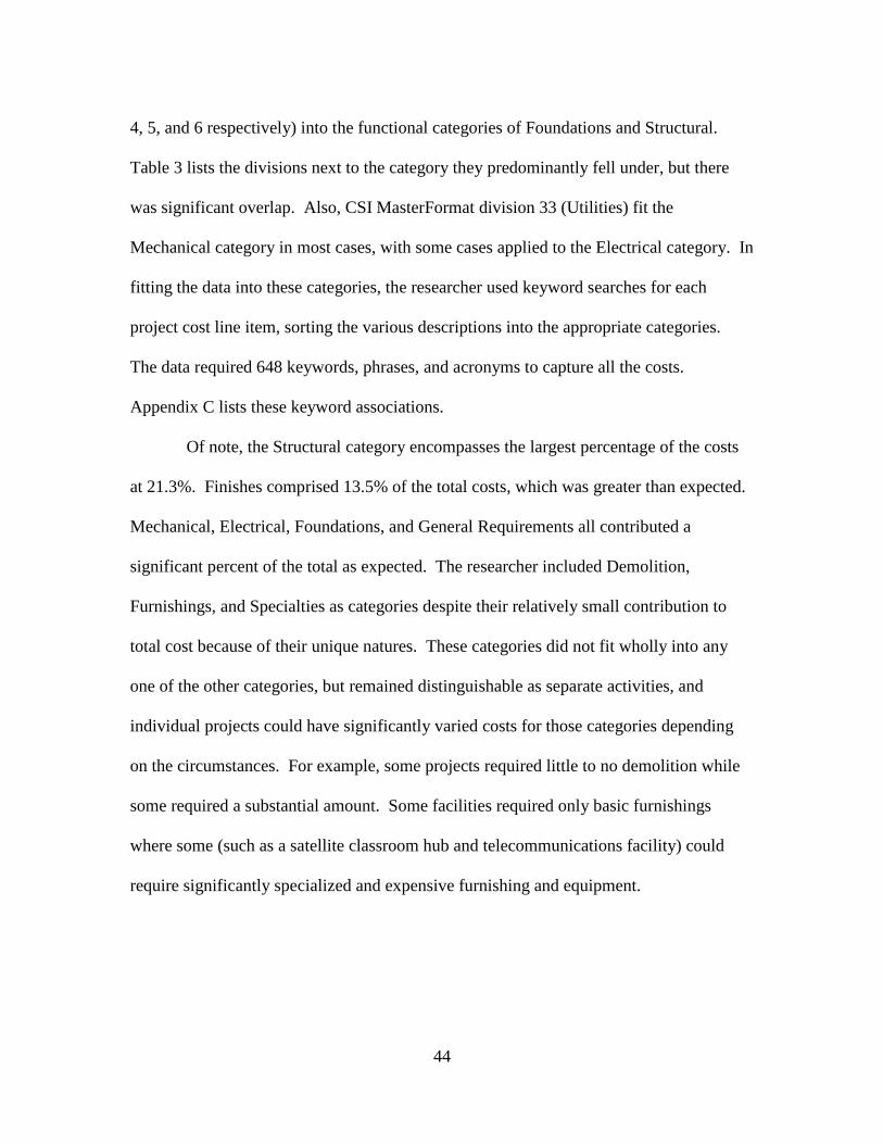
44
4, 5, and 6 respectively) into the functional categories of Foundations and Structural.
Table 3 lists the divisions next to the category they predominantly fell under, but there
was significant overlap. Also, CSI MasterFormat division 33 (Utilities) fit the
Mechanical category in most cases, with some cases applied to the Electrical category. In
fitting the data into these categories, the researcher used keyword searches for each
project cost line item, sorting the various descriptions into the appropriate categories.
The data required 648 keywords, phrases, and acronyms to capture all the costs.
Appendix C lists these keyword associations.
Of note, the Structural category encompasses the largest percentage of the costs
at 21.3%. Finishes comprised 13.5% of the total costs, which was greater than expected.
Mechanical, Electrical, Foundations, and General Requirements all contributed a
significant percent of the total as expected. The researcher included Demolition,
Furnishings, and Specialties as categories despite their relatively small contribution to
total cost because of their unique natures. These categories did not fit wholly into any
one of the other categories, but remained distinguishable as separate activities, and
individual projects could have significantly varied costs for those categories depending
on the circumstances. For example, some projects required little to no demolition while
some required a substantial amount. Some facilities required only basic furnishings
where some (such as a satellite classroom hub and telecommunications facility) could
require significantly specialized and expensive furnishing and equipment.
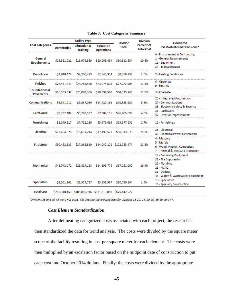
45
Table 3: Cost Categories Summary
Cost Element Standardization
After delineating categorized costs associated with each project, the researcher
then standardized the data for trend analysis. The costs were divided by the square meter
scope of the facility resulting in cost per square meter for each element. The costs were
then multiplied by an escalation factor based on the midpoint date of construction to put
each cost into October 2014 dollars. Finally, the costs were divided by the appropriate
46
Area Cost Factor for the project location, placing the costs at a standardized location
index of 1 to adjust for differences in construction costs throughout the U.S. UFC 3-701-
01 provided both the escalation rates and Area Cost Factors for these adjustments
(Department of Defense, 2015). Appendix B displays the project costs and scopes along
with the standardized costs. At this point, the researcher used a random number
generator to select one project from the dormitories category and two projects each from
the education and training category and squadron operations category and set them aside
for validation of the model after creating and running the simulation. Therefore, 7
dormitory projects, 18 education and training projects, and 13 squadron operations
projects were used to build the cost estimation model.
Distribution Modeling
Using the now-standardized cost data, the researcher modeled distributions and
correlations for each of the three facility types. While the lognormal distribution was
expected based on prior research (Touran & Wiser, 1992; Wall, 1997), the generalized
beta distribution modeled all the cost distributions more closely. The analysis revealed
the lognormal distribution as the next most feasible choice in most cases, but it did not
pass the Kolmogorov-Smirnov Goodness of Fit test. The data did not allow for a Chi-
Squared Goodness of Fit test because the test requires binning the data in such a way that
the sample size multiplied by the bin probability is greater than five (Frey & Cullen,
1995). A maximum sample of 18 in the case of the education and training facility type
allowed the formation of only three bins, limiting the viability of the Chi-Squared test.
Therefore, the researcher turned to the Kolmogorov-Smirnov Goodness of Fit test
instead.

47
The Kolmogorov-Smirnov test statistic indicated there was not sufficient evidence
to reject the hypothesis that the data came from a generalized beta distribution for all cost
categories of the dormitory, education and training and squadron operations types. The
General Requirements category for dormitories had the highest Kolmogorov-Smirnov
test statistic with a D of 0.437, resulting in a p-value of 0.099. Because the p-value was
greater than the α of 0.05, the hypothesis that the underlying distribution was the
generalized beta was not rejected. This value was the lowest p-value of the various cost
elements; all others had a higher p-value, reinforcing the generalized beta as viable
distribution candidate. Additionally, none of the other distributions considered had a
passing test statistic, despite the lognormal distribution coming close to a passing p-value
for a few elements. The gamma distribution followed the generalized beta distribution as
the next closest distribution for one cost element but again did not pass the goodness of
fit test. Therefore, the researcher kept the generalized beta and the associated parameters
for those cost elements for the simulation modeling. This decision is supported by prior
research stating the beta distribution is still a viable distribution to use when estimating
construction element costs (Chau, 1995b; Touran & Suphot, 1997; Yang, 2005).
Appendix B displays the test statistics and associated p-values for each cost element.
Correlation Modeling
After defining the distributions, a Spearman rank correlation function provided
the basic correlation matrices between the cost elements for each facility type. The
education and training correlation matrix and the squadron operations correlation matrix
were both positive definite, necessitating no further changes. The dormitory correlation
matrix was only semi-definite and had a negative eigenvalue, requiring modification
48
before it could correlate random variables. A nearest positive definite matrix function
from Higham’s (2002) algorithm provided the necessary modifications resulting in a
feasible matrix. The new correlation matrix was similar to the initially calculated matrix
but with the correlations altered an average of 2.59 x 10⁻⁸
, the largest adjustment of which
was 7.20 x 10⁻⁸
. These adjustments were in both the positive and negative direction. As
this maintained the overall correlation structure with minimal changes, the simulation
used the revised correlation matrix. Furthermore, Spearman rank correlations of the
simulation results provided an additional validation of the process. The correlations of
the facility cost distribution outputs were within 0.0117 of the original input correlations
on average, with a maximum difference of 0.0195. Therefore, the simulation kept the
cost elements correlated as desired with only minor variations. Appendix B annotates all
three correlation matrices used in the simulation.
Simulation Modeling
The researcher input the modeled distributions and feasible correlation matrices
into the Monte Carlo simulation, running each simulation 100,000 times. The trials
resulted in three predictive probability histograms for project construction costs of the
facility types of dormitories, training and education facilities, and squadron operations
facilities. The earlier cost element standardization steps aligned these probability
histograms in terms of dollars per square meter, using October 2014 dollars, with a
generic Area Cost Factor of 1. As described in Chapter I, the purpose of this research
was to develop a model relying only on basic scope information such as square meter
project area, creating an improved AACE Class 4 estimate model with an expected
accuracy of -15% to +25%.

49
Model Validation
Validation of this model consisted of applying the simulation to estimate the costs
of five reserved data samples to evaluate its predictive capability. The validation
compared these five outputs to three other estimates. The first estimate was the
programmed amount (PA), a Class 2 or 1 estimate, depending on the level of design
accomplished before the estimation. Cost estimators can create a Class 2 estimate after
designing the project to the 35% level or greater, and they can create a Class 1 estimate
after designing the project to the 70% level or greater. Generally, a PA relies on a 35% to
65% design, resulting in an estimate in the Class 2 category with an expected accuracy
within -7.5% to +10% of the actual project costs. Since this model is a Class 4 estimate,
the PA provided the most stringent standard of measurement, as it was a higher estimate
Class type with greater expected accuracy than the model.
The second and third estimates used in the validation process were Class 4
estimates based on the square meter scope of the projects. As Class 4 estimates, their
expected accuracy was within -15% to +25% and was, therefore, the same Class as the
model developed in this research. UFC 3-701-01 DoD Facilities Pricing Guide (2015)
developed the first of these and outlines criteria for applying unit costs by facility type in
Chapter 2 and adjustment factors in Chapter 4. The AFCESA Historical Air Force
Construction Cost Handbook validated the other estimate and outlines similar criteria as
the UFC in Sections II and IV–VI (2007).
The researcher took the three facility-type probability histograms and applied the
reserved five data samples to validate the model (one sample was of the dormitory
facility type, two were of the education and training type, and two were of the squadron
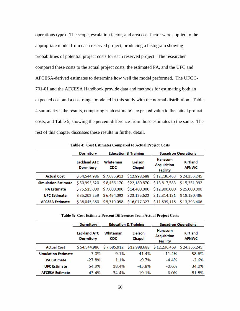
50
operations type). The scope, escalation factor, and area cost factor were applied to the
appropriate model from each reserved project, producing a histogram showing
probabilities of potential project costs for each reserved project. The researcher
compared these costs to the actual project costs, the estimated PA, and the UFC and
AFCESA-derived estimates to determine how well the model performed. The UFC 3-
701-01 and the AFCESA Handbook provide data and methods for estimating both an
expected cost and a cost range, modeled in this study with the normal distribution. Table
4 summarizes the results, comparing each estimate’s expected value to the actual project
costs, and Table 5, showing the percent difference from those estimates to the same. The
rest of this chapter discusses these results in further detail.
Table 4: Cost Estimates Compared to Actual Project Costs
Table 5: Cost Estimate Percent Differences from Actual Project Costs

51
Dormitory Project Cost Estimation
The dormitory estimation results revealed the model as a better predictor of costs
than the programmed estimate in the case of the one project reserved for validation. The
Lackland AFB, TX Airmen Training Complex Dormitory was randomly selected as the
validation project. This dormitory spanned 21,544 square meters and was built in 2009.
Figure 3 shows the simulation results in the form of a histogram, with the 50th
percentile
marked for reference. Figure 3 also has the actual project value along with the PA
estimate and estimated cost distributions from the UFC 3-701-01 DoD Facilities Pricing
Guide (2015) and the AFCESA Historical Air Force Construction Cost Handbook (2007)
overlaid on the histogram for comparison. The actual project cost of $54,544,986 was
located slightly above the simulated 50th
percentile of $50,993,620 and below the 75th
percentile of $58,234,100. This accuracy is significantly more accurate than the PA
estimate of $75,515,000, with the actual cost 7.0% higher than the model estimate
compared to 27.8% lower than the programmed amount estimate. The model came
within the Class 4 expected accuracy range of -15% to +25% whereas the PA did not
even meet the Class 4 estimate expectations despite being a Class 2 estimate. However,
it is also worth noting that of the seven dormitory projects used to create the underlying
model, one was a companion project dormitory, identical in scope to the one estimated
here and built on Lackland AFB in 2010. Having a similar project with comparable costs
embedded in the model likely improved the estimate for this particular validation more
than estimating for a project without such close similarities.

52
In comparing the simulation model results to estimates derived from UFC 3-701-1
and the AFCESA Handbook, the model produced more accurate results. The UFC 3-
701-1 estimate was $35,202,259, compared to which the actual cost was 54.9% higher
and, therefore, did not come within the Class 4 expected accuracy. The AFCESA
Handbook estimate was $38,045,360, compared to which the actual cost was 43.4%
higher, also outside the Class 4 accuracy range. Interestingly, both these estimates were
relatively close in their values to each other but far from the PA estimate, compared to
which the actual cost was 27.8% less. This discrepancy suggests that perhaps cost
estimators used different information when they prepared the estimate. The project was
significantly more costly than the average dormitory, suggesting the presence of cost
factors for which an estimator could account, but not to the extent the PA estimated.
Figure 3: Lackland ATC Dormitory Simulation Results and Cost Estimate Comparison

53
Education and Training Project Cost Estimation
The education and training facility results showed a useful, but potentially less
accurate, model. The graph in Figure 4 displays the simulation cost estimate histogram
with the project’s actual cost and the alternative cost estimates for the 2,540 square meter
Whiteman AFB, MO Child Development Center (CDC) built in 2005. The model
provided a useful prediction of the CDC costs with a 50th percentile estimate of
$8,456,170 compared to the actual cost of $7,685,912; a -9.1% difference, which lies
within the Class 4 accuracy range. The PA was a better estimate at $7,600,000,
compared to which the actual cost was only 1.1% higher, and, therefore, the PA was well
within the Class 2 accuracy range or -7.5% and +10%.
Both the UFC 3-701-01 and the AFCESA Handbook estimates were less accurate
than the PA and the simulation estimate. The UFC 3-701-01 estimate was $6,494,092,
just outside the Class 4 accuracy range with the actual cost 18.4% higher than estimated,
and the AFCESA Handbook estimate was $5,719,058, also outside the Class 4 range with
the actual cost 34.4% higher than estimated. In summary, the simulation estimated the
highest and was the only estimate higher than the actual cost, but the simulation still
performed better than the UFC or AFCESA methods. The PA was the best estimate
overall.
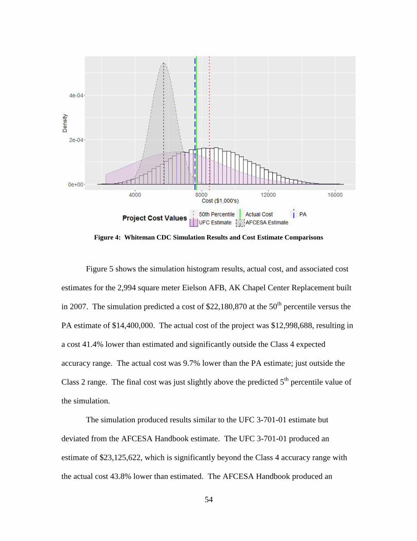
54
Figure 4: Whiteman CDC Simulation Results and Cost Estimate Comparisons
Figure 5 shows the simulation histogram results, actual cost, and associated cost
estimates for the 2,994 square meter Eielson AFB, AK Chapel Center Replacement built
in 2007. The simulation predicted a cost of $22,180,870 at the 50th
percentile versus the
PA estimate of $14,400,000. The actual cost of the project was $12,998,688, resulting in
a cost 41.4% lower than estimated and significantly outside the Class 4 expected
accuracy range. The actual cost was 9.7% lower than the PA estimate; just outside the
Class 2 range. The final cost was just slightly above the predicted 5th
percentile value of
the simulation.
The simulation produced results similar to the UFC 3-701-01 estimate but
deviated from the AFCESA Handbook estimate. The UFC 3-701-01 produced an
estimate of $23,125,622, which is significantly beyond the Class 4 accuracy range with
the actual cost 43.8% lower than estimated. The AFCESA Handbook produced an
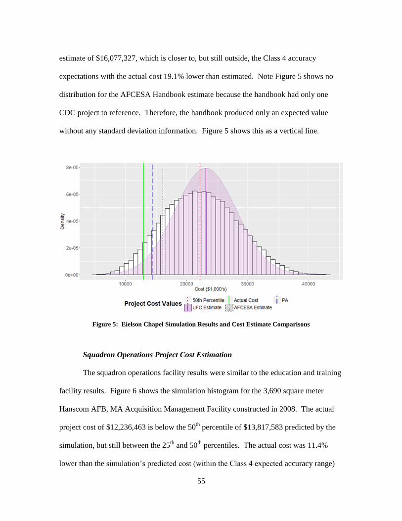
55
estimate of $16,077,327, which is closer to, but still outside, the Class 4 accuracy
expectations with the actual cost 19.1% lower than estimated. Note Figure 5 shows no
distribution for the AFCESA Handbook estimate because the handbook had only one
CDC project to reference. Therefore, the handbook produced only an expected value
without any standard deviation information. Figure 5 shows this as a vertical line.
Figure 5: Eielson Chapel Simulation Results and Cost Estimate Comparisons
Squadron Operations Project Cost Estimation
The squadron operations facility results were similar to the education and training
facility results. Figure 6 shows the simulation histogram for the 3,690 square meter
Hanscom AFB, MA Acquisition Management Facility constructed in 2008. The actual
project cost of $12,236,463 is below the 50th
percentile of $13,817,583 predicted by the
simulation, but still between the 25th
and 50th
percentiles. The actual cost was 11.4%
lower than the simulation’s predicted cost (within the Class 4 expected accuracy range)
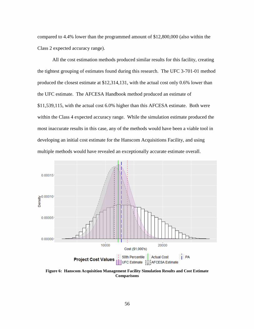
56
compared to 4.4% lower than the programmed amount of $12,800,000 (also within the
Class 2 expected accuracy range).
All the cost estimation methods produced similar results for this facility, creating
the tightest grouping of estimates found during this research. The UFC 3-701-01 method
produced the closest estimate at $12,314,131, with the actual cost only 0.6% lower than
the UFC estimate. The AFCESA Handbook method produced an estimate of
$11,539,115, with the actual cost 6.0% higher than this AFCESA estimate. Both were
within the Class 4 expected accuracy range. While the simulation estimate produced the
most inaccurate results in this case, any of the methods would have been a viable tool in
developing an initial cost estimate for the Hanscom Acquisitions Facility, and using
multiple methods would have revealed an exceptionally accurate estimate overall.
Figure 6: Hanscom Acquisition Management Facility Simulation Results and Cost Estimate
Comparisons
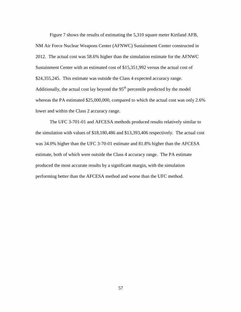
57
Figure 7 shows the results of estimating the 5,310 square meter Kirtland AFB,
NM Air Force Nuclear Weapons Center (AFNWC) Sustainment Center constructed in
2012. The actual cost was 58.6% higher than the simulation estimate for the AFNWC
Sustainment Center with an estimated cost of $15,351,992 versus the actual cost of
$24,355,245. This estimate was outside the Class 4 expected accuracy range.
Additionally, the actual cost lay beyond the 95th
percentile predicted by the model
whereas the PA estimated $25,000,000, compared to which the actual cost was only 2.6%
lower and within the Class 2 accuracy range.
The UFC 3-701-01 and AFCESA methods produced results relatively similar to
the simulation with values of $18,180,486 and $13,393,406 respectively. The actual cost
was 34.0% higher than the UFC 3-70-01 estimate and 81.8% higher than the AFCESA
estimate, both of which were outside the Class 4 accuracy range. The PA estimate
produced the most accurate results by a significant margin, with the simulation
performing better than the AFCESA method and worse than the UFC method.

58
Figure 7: Kirtland AFNWC Sustainment Center Simulation Results and Cost Estimate
Comparisons
In summary, the results did not produce a clear trend between the estimation
methods. However, of the five facilities tested, the simulation results performed better
than the UFC and AFCESA estimates twice, performed better than one of them but not
the other twice, and performed worse than both once. In the one case the simulation
performed worse, all the estimates formed a relatively concentrated grouping with all
estimates well within the Class 4 accuracy range and the simulation estimate producing a
result compared to which the actual cost was 11.4% lower. While the data available
allowed only limited validation testing, the simulation performed well overall and for the
dormitory estimate in particular. These results indicate the possible future utility of
developing this model further for initial cost estimating. Figure 8 highlights the
performance of this model, showing the accuracy of each estimate compared to the
projects’ actual costs and the Class 4 expected accuracy range.

59
Figure 8: Accuracy Comparison between Cost Estimates
Investigative Questions Answered
This research began by trying to answer the following three questions, with the
goal of providing additional insight into the behavior of Air Force construction cost
elements and methods for leveraging those behaviors for improved initial cost estimates.
This is what the research found:
Question 1
What distributions can adequately describe cost trends in construction project
assembly items?
While the literature predominantly supported using the lognormal distribution for
construction cost elements, this study found that the generalized beta distribution better
fit the data available. This result is understandable given the small sample sizes used and
the greater flexibility of the generalize beta to fit a wide range of shapes over the
lognormal. However, because the analysis revealed the lognormal distribution as the next
60
best distribution option for many of the cost elements, the researcher proposes that
additional data may refine the overall cost shape, resulting in the lognormal distribution
possibly becoming a better fit. Nevertheless, the predictive potential of the model as
shown in the final results indicate that the generalized beta distribution may provide the
resolution required for a viable model without necessitating a switch to the lognormal
distribution.
Question 2
How do correlations between assembly items affect overall project costs?
The literature strongly supported the assertion that correlations between cost
elements have a significant impact on final cost and should always be included if
possible. This research supported that premise, with the data revealing significant
correlations between the 11 cost elements modeled.
Question 3
How does a Monte Carlo cost simulation model using historical cost distributions
differ in performance from the current parametric cost estimation method?
For the case of dormitory facility projections, the simulation modeled in this
research performed substantially better than the programmed parametric cost estimate,
the UFC 3-701-01, and AFCESA Construction Cost Handbook for the one project tested.
For the education and training facility and squadron operations facility projections, the
simulation did not out-perform the programmed cost estimate in any of the four tests, but
still provided a useful approximation in one of the two cases tested for each facility type.
Nevertheless, even in the other two cases for which the actual costs fell close to the outer

61
5% probability prediction values, the model showed value and still performed better than
the UFC method in one case, and the AFCESA method in the other.
The model showed potential in providing a usable range of expected values for a
given project type. Initial program estimates should fall within the middle 50% of the
model. If they fall well below that, as was the case for the Eielson AFB Chapel, there
should be reasoning behind the low estimate. The fact that the Eielson AFB Chapel had
the third lowest cost per square meter of all the projects analyzed supports this reasoning,
indicating some project-specific attributes contributing to a lower-than-normal cost.
Indeed, the Chapel had lower-than-average costs for each of the 11 cost elements and was
one of only two education and training facilities for which the researcher collected data
that did not require any demolition. Taking this into consideration, a valuable future
improvement to the model developed here would be to include the capability of removing
or adjusting the costs of individual elements depending on project-specific conditions.
Furthermore, the Chapel was one of two projects based in Alaska, both of which had cost
per square meter values in the bottom 16% of all project data collected after adjusting for
location factors. This fact indicates a possible systemic factor causing a reduction in
relative cost.
If the initial program cost estimate falls well above the middle 50% of the model,
there should be reasoning for those higher costs. For the Kirtland AFB AFNWC
Sustainment Center project, the cost per square meter was third highest among the
projects analyzed. Furthermore, the communication cost per square meter was over
double the cost of the next highest communication cost for any of the other projects
regardless of facility type. Clearly, the AFNWC Sustainment Center had a significant
62
communications requirement above the standard, necessitating a cost estimate higher
than the average.
Summary
The results of this research provide significant insight into cost estimation. The
proposed simulation produced an empirical model useful for bounding and checking
initial cost estimates. Collecting enough data and applying a viable methodology to
model cost element distributions and correlations were crucial to a successful simulation.

63
V. Conclusions and Recommendations
Chapter Overview
The Monte Carlo simulation developed in this research provided a new cost
estimation tool with potential utility for preliminary Air Force construction cost
estimation. This chapter outlines these results and their implications. The first section of
the chapter provides a summary of the research conclusions. Next, the chapter covers
limitations of the research followed by the significance of the research. Finally, the
chapter discusses recommendations for both action and future research to continue and
expand the work presented in this paper.
Conclusions of Research
This study provided some useful insights into Air Force construction cost
estimation modeling. The generalized beta distribution proved to be a viable distribution
for cost element modeling, with the lognormal distribution remaining as a possible
alternative, particularly if more data become available to test its utility. Correlations
between cost elements affected overall cost estimates significantly, as emphasized in past
research and by the correlations found in this research. Additionally, the Monte Carlo
simulation revealed a given project’s range of probable costs, highlighting well the cost
estimate’s uncertainty and allowing for the selection of an estimate at the desired percent
confidence level. These attributes provide significant benefits over the UFC or AFCESA
estimation models, and even over the PACES framework used for estimates at later
design phases. PACES, UFC, and AFCESA all assume normal distributions for their cost
data and do not correlate internal elements. Using a more accurate distribution such as
64
the generalized beta and correlating major cost elements significantly improves a model’s
ability to simulate actual project cost effects. With a larger data set to refine the model in
this research, the simulation’s accuracy could improve substantially.
Specifically for the validation projects tested, this research provided an accurate
cost estimation tool in three of the five cases. For the dormitory project, the model
developed here performed significantly better than any other estimate tested, including
the programmed amount. For one project each within the education and training projects
and the squadron operations projects, this research’s model performed well within the -
15% to +25% accuracy range desired. For the other project in each category, this model
did not fall within the desired accuracy range, but still performed better than one other
measure in each case. Furthermore, the projects for which the model did not provide as
accurate of predictions had possible unique factors, which may have contributed to costs
deviating significantly from the model’s expected value.
Limitations of Research
The key limitations of this research centered on a lack of data. The model was
able to produce significant results; however, additional data could have improved the
accuracy of the distribution and correlation modeling, leading to potentially more
accurate results. Moreover, added data would have allowed the modeling of additional
facility types, along with further testing and validation of those facility-type models.
Testing the dormitory model with only one project and the education and training along
with the squadron operations models with only two projects each limited the validation of
this research.
65
Significance of Research
There are two significant ramifications from this research. First, this model
provided a methodology to create a viable tool in early cost estimation efforts,
highlighting not only a likely cost but also the range of expected costs and their
associated uncertainty. The correlated cost element modeling and simulation developed
here were overall as effective as other comparable preliminary cost estimation methods
for the projects tested even with limited data, and they better reflected actual cost element
characteristics. Second, this research showed the relative accuracy for currently-used
estimation methods. The variation of the estimates reveals that the methods may not be
consistently producing estimates within the accuracy expected of their given estimation
class. Further work in cost estimation may be warranted judging by these results. The
model developed here may provide a comparison estimate or an alternative means for
improving preliminary cost estimation.
Recommendations for Action
The model developed in this research, if expanded, could integrate into the Air
Force’s primary cost estimation tool, PACES, for initial cost estimation. Instead of only
creating initial estimates using historical data for average costs per square foot/square
meter, the same project scope information could fuel a correlated cost-element Monte
Carlo simulation, providing further insight into potential project costs. Having a
probability distribution of likely costs as an additional estimate tool could give estimators
greater insight into the project’s inherent cost risks and provide a secondary check to
other estimation methods. Then, by programming the probability cost profile into the
project file to some degree, instead of only recording a point estimate, decision-makers

66
would have additional useful information when selecting projects for execution and
allocating funds.
Issues with such an implementation also lie in data collection, however. In this
research, the dormitory model relied on the smallest sample size of eight projects total,
with one reserved for validation leaving seven for model development. Such a small
sample size is not ideal for developing the model, and at least that many projects per
facility type would be required to expand the model to other facility categories. Due to
the wide variation in Air Force facilities, this data collection effort would be substantial.
However, the UFC and PACES cost estimation models require some level of data
collection currently. Therefore, these collection procedures could expand to meet the
parameters for data to support a method similar to this research. As enough project data
became available, the model could be expanded facility type by facility type, providing
utility in the order of the most-often constructed types as the Air Force completes and
documents projects. Not only would such data support the model developed here, but
would be useful for other cost research and analysis in the continual effort to improve the
Air Force’s cost estimation models.
Recommendations for Future Research
Future research could build upon this study in several ways. First, a future
researcher could expand the model, validating and refining the results to include
additional facility types. In particular, modeling airfield-related projects would add a
crucial element to the scope of this research line as the airfield is the most critical asset of
an Air Force installation. Additionally, follow-on research could compare the results to
initial parametric models from PACES or RSMeans estimates for further insight. Data

67
for an effort such as this would likely come from the United States Army Corps of
Engineer’s Resident Management System, but may suffer from the same data limitations
as discussed for the research in this paper. However, both the Army and Navy construct
many facility types in common with the Air Force, and collecting those projects may
prove useful in aggregating a larger sample size for analysis.
Second, a future researcher could modify and refine the general methodology
used here for military construction projects and instead apply to facility sustainment,
restoration, and modernization (FSRM) projects. The Air Force’s Automated Civil
Engineer System may contain the requisite data for the numerous FSRM projects
documented therein. A future researcher could then build and analyze a similar model to
this research for these smaller-scoped but more numerous projects constructed in the Air
Force. Data quality may be a significant issue, but the utility of an application of this
type would be considerable due to the large amount of FSRM projects requiring cost
estimates.
Summary
This research succeeded in developing a relatively accurate Class 4 cost
estimation method. The model, while not always more accurate than the standard
parametric cost estimates in all cases, produced results useful for the cost estimation
process with implications for improving current estimation practices. This method also
revealed the range of uncertainty in the estimate for decision makers to evaluate risk,
while only requiring knowledge of basic scope parameters for a given project.
Additionally, the research provided insight into distribution modeling and correlation of
cost elements, while validating the use of a Monte Carlo simulation to estimate costs.

68
Overall, these insights into Air Force construction costs and the subsequent model
expand the foundation for future research and cost estimation practice development.
Building on these methods, the Air Force can produce increasingly accurate estimates
with a picture of the inherent risks and cost probabilities.
69
Appendix A: Construction Cost Research White Paper
White Paper: Report for AFCEC on Air Force Construction Cost Research
The following white paper was developed for the Air Force Civil Engineer Center
(AFCEC) to provide a summary of Air Force research conducted in the realm of
construction costs. The white paper focuses on Air Force Institute of Technology
research and includes studies from 1986-2015. The research covers four main topics:
historical cost trend analysis; parametric estimation models; contract method evaluations;
and program-wide MILCON investigations. While not the primary focus of this research,
contract method evaluation and program-wide MILCON investigation topics are included
as an overview of the breadth of research related to construction costs. Historical cost
trend analysis and parametric estimation model topics are of primary concern here as they
relate to the development of specific project cost estimates prior to contracting the
construction work.

70
AIR FORCE CONSTRUCTION COST RESEARCH SUMMARY
Developed for the Air Force Civil Engineer Center
By Captain Jeffrey D. Buchholtz
I. Overview
The Air Force Institute of Technology (AFIT) has conducted numerous research
initiatives in identifying and analyzing trends, models, and methods related to
construction costs. In an effort to consolidate and synthesize those efforts for the Air
Force Civil Engineering Center (AFCEC), a brief summary of each research effort’s
scope and results are outlined and categorized into four main topics: historical cost trend
analyses, parametric estimation models, contract method evaluations, and program-wide
MILCON investigations. For additional references, Appendix A-1 lists the bibliographic
information and abstracts from each study, sorted alphabetically by author’s last name.
II. Research
1. Historical Cost Trend Analyses
Statistical analysis of trends within archived project data reveals factors that have
significant impact on cost. Awareness of these critical factors allows tracking and the
application of potential risk mitigation strategies to minimize negative influences or
manage areas of likely cost growth. One theme throughout the studies is the quality of
government personnel contract management significantly impacts overall construction
performance. Recommendations include minimizing government delays, increasing
communication and cooperation, and improving project definition with the user before
construction begins.
71
1.1. Analysis of Air Force Wartime Contracted Construction Project Performance
Hoff, Ryan M. – 2015 – AFIT Thesis
SCOPE: Captain Hoff analyzed factors for success and differing outcomes based on
contract type for 25 AFCEC construction projects in Afghanistan. The projects
consisted of reimbursable contracts and fixed-price contracts.
RESULTS: For general performance, government delays significantly impacted cost and
schedule while project management issues also impacted schedule. Notably,
weather and wartime security did not prove to be factors significantly impacting
cost or schedule. For contract type, reimbursable contracts had higher cost and
schedule growth, whereas fixed-price contracts did poorly in design performance
and contract management. Neither contract type showed a difference in quality.
As a result, Captain Hoff recommended the construction agent monitor cost and
project management closely for reimbursable projects, possibly by tracking
incremental progress and checking for excess labor, hours, or resources added to
the project. For fixed-price contracts, construction agents could use Lean
Analysis to identify sources of rework, inefficient process, and excess
requirements.
1.2. An Analysis of Cost Premiums and Losses Associated with USAF Military
Construction
Blomberg, Daniel L. – 2013 – AFIT Thesis
SCOPE: Captain Blomberg conducted a case-study of two nearly identical projects
constructed in 2009 on Joint Base Elmendorf-Richardson, Alaska, analyzing the
differences between the contract methods and management. One project was a
standard Design-Build project managed by the Unites States Army Corps of

72
Engineers (USACE) and the other project was a Design-Build pre-engineered
building managed by the 673rd
Civil Engineer Group (CEG) and AFCEC. These
results were compared to a survey of 18 respondents comprising of construction
and contract specialists from USACE, USAF and civilian contractors. Separately,
Captain Blomberg conducted a geospatial analysis, validated with a multivariate
analysis of the variance, to determine if the Davis-Bacon Act wage rates were
higher than local area wage rates, contributing to MILCON cost premiums.
RESULTS: The CEG-managed project cost 27% less and was completed in less than half
the time of the standard Design-Build project. This study validated that cost
premiums do exist for MILCON and highlighted 11 major factors causing those
premiums. In general, DoD actions and internal policies cause 80% of the
premiums while public law and the Federal Acquisition Regulations account for
20%. Additionally, the study revealed that Davis-Bacon Act wage rates were
higher than local wage rates. To mitigate some of these excess costs, Captain
Blomberg recommended improving cooperation between all agencies involved by
balancing risk, minimizing restrictive specifications, and encouraging innovation
toward the actual end product instead of toward a specific construction or contract
method.
1.3. An Analysis of Construction Cost and Schedule
Beach, Michael J. – 2008 – AFIT Thesis
SCOPE: Major Beach statistically analyzed 1,322 Air Force MILCON projects,
completed within the years 1990 to 2005 (excluding military family housing and
Non-Appropriated Funds projects) to determine if the project’s Major Command

73
(MAJCOM), construction agent, or category code (CATCODE) predicted cost or
schedule performance compared to the initial project estimates.
RESULTS: The MAJCOM and construction agent over a particular project did predict
cost and schedule performance, whereas CATCODE did not. In particular,
Pacific Air Forces MILCON projects managed by the USACE Alaska District
were consistently completed under the projected time and budget. In contrast, this
same agency did not perform favorably in Captain Blomberg’s case study.
Comparatively, the Air Force Center for Engineering and the Environment
(AFCEE) and the USACE European District were able to minimize cost growth,
but not schedule growth. Also, Air Combat Command’s projects tended to
perform well schedule-wise, regardless of the construction agent. While this
study highlighted MAJCOM and construction agent correlations with cost and
schedule, root causes were not identified.
1.4. Characterizing Patterns of MILCON Project Contract Modification
Nielsen, Tyler K. – 2007 – AFIT Thesis
SCOPE: Captain Nielsen statistically analyzed 278 Air Force MILCON Projects with
3,842 change orders, completed from 2000 to 2004 and obtained from the
Automated Civil Engineer System (ACES) database to reveal major causes of
change orders. He used the same source data used in Captain Jason Cook’s 2006
AFIT thesis.
RESULTS: Design deficiencies, followed by user change requests, were the largest
contributors to contract modifications. Significantly less so but still notable were,
in descending order, weather, scope deletion, and unforeseen site conditions.
74
Project managers could use these results to focus on the identified major
contributors to change orders in an effort to reduce their occurrences or minimize
their impact to cost and schedule growth.
2. Parametric Estimation Models
The following two studies developed parametric models using predictive factors
to estimate a future project’s cost based on past project trends or expert opinions. Of the
two studies, only one is recent enough to provide relevant insight into current cost
estimation issues.
2.1. Estimating Required Contingency Funds for Construction Projects Using
Multiple Linear Regression
Cook, Jason J. – 2006 – AFIT Thesis
SCOPE: Captain Cook created a model to predict contingency funds needed for a
construction project, using 218 Air Force MILCON projects to build the model
and reserving an additional 25 projects to validate the model once complete. The
projects were pulled from the ACES database and included a wide variety of
projects up to 2005.
RESULTS: Captain Cook found ten factors that combined to form a predictive model for
cost estimation. Specifically, the model calculates the estimated percent the
project will cost over the base estimate, thereby predicting the amount of
contingency funds needed. This model had an average error of 0.3% from the 25
projects used for validation and is as follows:
75
Ln (% Overrun) = -2.151-19.285x1 + 1.018 x2 + 0.140 x3 + 0.133 x4 – 0.216 x5 –
0.234 x6 – 1.008 x7 – 0.696 x8 – 0.958 x9 + 0.295 x10
Where
x1 = normalized design length (design length divided by the design cost)
x2 = estimate % of cost at award (estimate amount divided by the cost at
award)
x3 = design cost/cost at award > 10% (1 if > 10% and 0 if ≤ 10%)
x4 = September award (1 if contract award in September and 0 if not)
x5 = high competition > 9 bidders (1 if >9 and 0 if ≤ 9)
x6 = FY 2000 and later (1if funded after October 1, 1999 and 0 if not)
x7 = estimate % of PA (estimate amount divided by the programmed
amount)
x8 = type of work is emergency MILCON–EEIC341 (1 if so and 0 if not)
x9 = type of work is housing - EEIC713 (1 if so and 0 if not)
x10 = design greater than 2 years (1 if > 2 years and 0 if ≤ 2 years)
2.2. Formulation of a Construction Cost Estimating Procedure to Aid Designers in
Preparing Detailed Construction Cost Estimates
Stark, Steven R. – 1986 – AFIT Thesis
SCOPE: Captain Stark surveyed 112 base-level Air Force civil engineers to determine
factors on cost for projects and their level of impact in three price categories: less
than $200,000, between $200,000 and $500,000, and greater than $500,000.
RESULTS: The result of this research was a cost estimating computer program with the
goal of reducing cost estimation time but not necessarily improving accuracy.
Accuracy of cost estimates at the time of this study was determined to be within
5-15% with the commonly used RS Means databases. The factors used by the
model center around the type and location of the construction project along with
items such as weather and the amount of competition among bidders. Because the
data is outdated and most of the factors have been included in current cost
estimation practices, this model is of little utility now. However, this study marks
76
the first Air Force research found to attempt to analyze and modify existing cost
estimate practices to achieve better results.
3. Contract Method Evaluations
Several studies have examined the effect a project’s contract type can have on
cost performance. Of these, two found inefficiencies and issues with the standard
Design-Bid-Build method, favoring more streamlined and relational methods with better
cost and schedule results. The other two studies highlighted areas needing improved
contract management in general, which were otherwise negatively influencing project
costs.
3.1. Firm Fixed Price and Cost Plus Fixed Fee Construction Contracts in Iraq and
Afghanistan
Jaszkowiak, Lindsay M. – 2012 – AFIT Thesis
SCOPE: Captain Jaszkowiak used two methods in her research. First, she conducted a
statistical analysis of 127 AFCEE projects in Iraq and Afghanistan constructed
from 2006-2010. Second, she synthesized factors from a survey of 20 civil
engineers and contract personnel from throughout the Air Force.
RESULTS: Overall, poor record-keeping of lessons learned contributed to internal
management issues and a lack of improvement over time in all areas. Firm Fixed
Price contracts appeared to have less percent cost and schedule growth compared
to Cost Plus Fixed Fee, but those findings were not statistically significant. Cost
Plus Fixed Fee contracts were perceived to outperform Firm Fixed Price contracts
77
in general, and in the area of quality in particular. However, final results
indicated no substantial advantage for either type.
3.2. An Analysis of the Design-Build Delivery Approach in Air Force Military
Construction
Rosner, James W. – 2008 – AFIT Thesis
SCOPE: Captain Rosner analyzed 835 projects constructed from 1996-2006, obtained
through the ACES database. Of those projects, 278 were accomplished through a
Design-Build method and 557 were accomplished through a Design-Bid-Build
method. His goal was to determine if the Design-Build method performs better
than the traditional Design-Bid-Build method.
RESULTS: Overall, the Design-Build method proved better in six of the eight
performance measures, particularly with less cost growth and fewer modifications
per million dollars. However, Design-Bid-Build methods seemed to be superior
with less schedule growth. Captain Rosner theorized this was due instead to the
timing built into the current MILCON process of fiscal year funding. Design-
Build methods may prove superior with process changes to take advantage of the
method’s strengths.
3.3. Risk-Based Decision Model for Determining the Applicability of an Earned
Value Management System in Construction
Workman, Mark D. – 2006 – AFIT Thesis
SCOPE: Major Workman gathered a series of in-depth survey data from three subject
matter experts to identify risk factors that significantly impacted a construction
project’s cost growth and their estimated probability of occurrence. Major
Workman then created a decision model for determining if Earned Value
78
Management practices should be applied to MILCON projects under $20 million
in response to a new policy requiring such an evaluation.
RESULTS: The study concluded if the model predicts cost growth of over 5%, the use of
earned value management is recommended. However, due to the resources
required for Earned Value Management, Maj Workman recommended its use
only on projects over $5 million and for which the risk of a cost growth over 5%
was substantial enough to warrant additional investment.
3.4. Cost Analysis between SABER and Design-Bid-Build Contracting Methods
Henry, Elwood – 2000 – AFIT Thesis
SCOPE: Captain Elwood analyzed data from 46 projects between Wright-Patterson AFB
and Holloman AFB consisting of 31 Simplified Acquisition of Base Engineering
Requirements (SABER) projects and 15 Design-Bid-Build projects. The projects
were accomplished between 1990 and 1999.
RESULTS: Both methods had a wide range of costs, but Design-Bid-Build projects
tended to cost more. Also, SABER projects at Wright-Patterson AFB had less
schedule growth than Design-Bid-Build. All other comparisons did not produce
statistically significant differences. Because of the small sample size of
comparable projects between only two bases, further studies would be required to
generalize the findings to the Air Force overall.
4. Program-Wide MILCON Investigations
The following studies have taken a boarder look at Air Force construction,
analyzing risks and inefficiencies with the MILCON system as a whole. These studies
provide insights in themes and areas of concern instead of specific cost drivers.

79
4.1. Risks Associated with Federal Construction Projects
Surajbally, Krishna R. – 2011 – AFIT Thesis
SCOPE: Captain Surajbally conducted a risk analysis of implementing Building
Information Modeling. He evaluated the risks in the areas of critical
infrastructure, information technology, contracting, and cost. The study focused
on Design-Build MILCON projects with the USACE as the construction agent,
using a literature review as the foundation for the analysis.
RESULTS: Captain Surajbally concluded that the most significant risks in implementing
Building Information Modeling are information technology related, but
management teams should balance the cost of accepting the risk versus
implementing mitigation measures.
4.2. A Proposed Military Construction Facility Investment Model
Dempsey, Andre R. – 2003 – AFIT Thesis
SCOPE: Major Dempsey used system dynamics and Value-Focused Thinking analysis
methods to evaluate the MILCON investment model and to recommend
improvements.
RESULTS: Major Dempsey created a MILCON investment model that was rated 92.02%
effective at targeting C-3 and C-4 requirements for funding, compared to the
existing model rated at 71.68%. The existing model allocated funds based on
each MAJCOM’s plant replacement value, average project costs, and number of
projects for which funds were requested. Instead, the proposed model allocated
funds directly based on C-3 and C-4 requirements and the age of facilities,
distributing funds where most needed instead of by relative portfolio size. While
80
this study aimed to provide a solution for the Air Force’s goal of eliminating C-3
and C-4 classified facility deficiencies by 2010, the program recommendations
may still be applied to improve current MILCON funding efficiency.
4.3. An Investigation Concerning Perceptions of Military Construction Program
Effectiveness
Dutcher, Gerald B. – 1986 – AFIT Thesis
SCOPE: Captain Dutcher surveyed 770 Air Force personnel at the Air Force Region
Civil Engineer agency, MAJCOMs, and various bases working with the Military
Construction Program for perceptions on primary inefficiencies.
RESULTS: Key inefficiencies identified were poor scope definition, lack of delegated
authority, length of time required to input project details (particularly in “Project
Books”), and breakdown in communications (particularly for special projects on a
short timeline).

81
Appendix A-1: Abstracts
Beach, Michael J., (2008). An Analysis of Construction Cost and Schedule.
Unpublished Masters Thesis, Air Force Institute of Technology, Wright
Patterson AFB OH.
ABSTRACT:
Cost and schedule performance are widely accepted in the literature and in
industry as effective measures of the success of the project management effort. Earned
Value Analysis (EVA) is one method to objectively measure project cost and schedule.
This research evaluates the cost and schedule performance of 1,322 completed United
States Air Force (AF) Military Construction (MILCON) projects, executed from 1990 to
2005. The impact of Major Command (MAJCOM), Construction Agent (CA), facility
type (CATCODE), individually and in combination, on the EVA metrics of Cost
Performance Index (CPI), Time Performance Index (TPI), and CPI*TPI were evaluated.
The results indicate that AF MILCON projects are typically executed either on or below
their respective budgets, but typically take more time than expected for construction. This
outcome implies that AF MILCON projects trade time performance in an effort to control
costs. When cost and performance are given equal weight, the sacrifice made in time
performance is greater than the benefit gained in cost performance.
Blomberg, Daniel L., (2013). An Analysis of Cost Premiums and Losses Associated
with USAF Military Construction. Unpublished Masters Thesis, Air Force
Institute of Technology, Wright Patterson AFB OH.
ABSTRACT:
Military construction (MILCON) represents 40% of the federal government’s $30
billion construction budget. The federal budget is fixed; therefore, any cost overages
likely affect project scope or requirements. This study investigated if MILCON
procurement costs more than private industry construction and if so, what causes the cost
premiums. A combination of in-depth literature review, expert interviews, a unique case
study, expert surveys, and geospatial statistical analysis answered the research question.
The case study evaluated two nearly identical projects to determine how internal factors,
in addition to public laws, affect MILCON cost premiums.
This study confirmed the existence of MILCON cost premiums. Additionally, 11
major cost premium themes emerged: overly restrictive statements of requirements,
failing to balance risk, stifling or not applying innovation, unique MILCON
requirements, parameterization of the execution process, selection of construction
specifications, schedule and submittal policies, perception of MILCON construction
agents, anti-terrorism/force protection requirements, Federal Acquisition Regulations,
and socioeconomic laws and policies. Additionally, in spite of the contract requirement
similarities, once complete, the studied projects differed by over a year of construction
time and $7 million. Research frequently cites federal laws and policies as the primary

82
cost premium driver; however, this research demonstrated internal construction policies,
which the military can control, also cause increased cost premiums.
Cook, Jason J., (2005). Estimating Required Contingency Funds for Construction
Projects Using Multiple Linear Regression. Unpublished Masters Thesis, Air
Force Institute of Technology, Wright Patterson AFB OH.
ABSTRACT:
Cost overruns are a critical problem for construction projects. The common
practice for dealing with cost overruns is the assignment of an arbitrary flat percentage of
the construction budget as a contingency fund. This research seeks to identify significant
factors that may influence, or serve as indicators of, potential cost overruns. The study
uses data on 243 construction projects over a full range of project types and scopes
gathered from an existing United States Air Force construction database. The author uses
multiple linear regression to analyze the data and compares the proposed model to the
common practice of assigning contingency funds. The multiple linear regression model
provides better predictions of actual cost overruns experienced. Based on the
performance metric used, the model sufficiently captures 44% of actual cost overruns
versus current practices capturing only 20%
The proposed model developed in this study only uses data that would be
available prior to the award of a construction contract. This allows the model to serve as a
planning tool throughout the concept and design phases. The model includes project
characteristics, design performance metrics, and contract award process influences. This
research supports prior findings of a relationship between design funding and design
performance as well as the influence of the contract award process on cost overruns.
While the proposed model captures 44% of actual cost overruns, its application reduces
average contingency budgeting error from -11.2% to only -0.3% over the entire test
sample.
Dempsey, Andre R., (2003). A Proposed Military Construction Facility Investment
Model. Unpublished Masters Thesis, Air Force Institute of Technology,
Wright Patterson AFB OH.
ABSTRACT:
The fiscal year (FY)1999 and FY2000 National Defense Authorization Acts
(NDAA) amended Title 10 USC, Section 17, and directed the secretary of defense to
report annually on the capability of installations and facilities to provide support to forces
in the conduct of their missions. This has come to be known as the Installations’
Readiness Report (IRR). The Air Force’s IRR links facility sustainment, restoration, and
modernization (SRM) requirements, with the impact on the installation’s ability to
support the mission associated with the particular facility class. The Air Force’s
centralized military construction (MILCON) program model used to program major
facility requirements does not directly target facility investment in the “deficient” facility
classes defined in the Installations’ Readiness Report.
83
This research combined the system dynamics and value-focused thinking
methodologies together to develop a proposed MILCON model that might better target
funding of deficient facility class requirements. The results from a system dynamics
analysis of the existing MILCON model were used to better understand the MILCON
program and leverage management policies in a proposed MILCON model. The proposed
MILCON model was then developed using a gold standard value-focused thinking
approach. The Air Force’s goals and objectives for the MILCON program were derived
from a literature review of key doctrine, policies, and guidance. The proposed model was
also evaluated to identify relevant favorable or unfavorable behavior trends in eliminating
deficient facility class requirements. The proposed model provides a significant short and
long-term improvement over the existing model in targeting and eliminating deficient
facility class requirements. The model demonstrates a 20 percent improvement in
targeting these facility requirements in FY2004 and a long-term trend towards completely
eliminating these requirements.
Dutcher, Gerald B., (1986). An Investigation Concerning Perceptions of Military
Construction Program Effectiveness. Unpublished Masters Thesis, Air Force
Institute of Technology, Wright Patterson AFB OH.
ABSTRACT:
In this thesis the primary inefficiencies of the Military Construction Program (MCP), as
commonly perceived by the Air Force Region Civil Engineer (AFRCE), the Major
Command (MAJCOM), and the bases are identified. These three management levels are
the primary managers of the MCP program. The MCP problems identified included
inadequate definition of scope at the inception of MCP projects, and ineffective technical
and functional design reviews.
Data was gathered from the AFRCE, the MAJCOM and the base through 770
questionnaires, mailed throughout the continental United States. All of the personnel
involved with the MCP were surveyed at the AFRCEs and MAJCOM. The base
personnel were randomly sampled.
The methodology used involved a one-way analysis of variance of the mean
responses, from the AFRCE, the MAJCOM and the base, to a seven point Likert scale.
Significant opinion differences were verified with the Scheffe test for all possible
comparisons.
Henry, Elwood, (2000). Cost Analysis between SABER and Design Bid Build
Contracting Methods. Unpublished Masters Thesis, Air Force Institute of
Technology, Wright Patterson AFB OH.
ABSTRACT:
The majority of Air Force construction performed by two main contractual
methods, Design Bid Build (DBB) and Simplified Acquisition of Base Engineering
Requirements (SABER). DBB is the traditional contracting method where each project is
84
competitively bid. SABER uses one contractor to complete multiple projects over the
duration of the contract, using unit prices established in the original contract.
The purpose of this research project was to perform a cost analysis between DBB
and SABER construction. The research involved finding appropriate projects completed
by the two methods that were comparable. This involved going to Wright-Patterson and
Holloman Air Force Bases to gather project information. There were a total of 46 projects
collected from both bases. Then a methodology was developed to compare the projects
collected. Projects were divided into categories containing similar types of construction.
Data from the project was then used to calculate a unit cost per dimensional characteristic
for the project. Project comparability was demonstrated by showing that the group of
projects constructed by each method completed a similar type and scope of work. Time
and cost growth were also compared for DBB versus SABER.
The research findings showed that SABER was cheaper but not at a statistical
level of significance. The comparison could only be completed in one area of
construction, interior renovation, due to the limited number of comparable projects in the
remaining construction categories. SABER construction also performed better in cost and
time growth for most instances.
Hoff, Ryan M., (2015). Analysis of Air Force Wartime Contracted Construction
Project Performance. Unpublished Masters Thesis, Air Force Institute of
Technology, Wright Patterson AFB OH.
ABSTRACT:
US-led construction projects in Afghanistan have performed poorly on-average;
indeed, it is the norm to deliver projects late to need and over budget to the customer.
Using a dataset of 25 Afghan wartime projects, we address two separate, yet related
questions relating to these DoD construction activities in the Afghan theater of
operations. These questions are: 1) What factors affect the success of construction
projects; and 2) How do project outcomes differ based on the contract type? First, with
regards to critical success factors, current literature suggests that wartime projects may
face the same cost and schedule factors as peacetime projects, with some notable
additions. Using peacetime factors as a baseline, project factors, health and safety
compliance, quality of work, technical performance, work productivity, and external
environmental factors were tested with contingency tables to determine if they are
predictive of schedule or cost performance. We found that external environmental
factors, to include weather and wartime security, were not predictive of project
performance. However, cost performance and schedule performance was found to be
significantly dependent on government-issued excusable delays. Moreover, project
management deficiencies were predictive of poor schedule performance but not cost
performance. Second with regards to contract type, as the Afghan security condition was
volatile, contracting officers dynamically used both reimbursable and fixed-price
contracts in order to accomplish the mission. Using the Mann-Whitney tests, performance
differences between contract types were explored. We found reimbursable contracts to
have significantly greater cost and schedule growth. Additionally, fixed price projects
were found to have more problems with design performance and contract management.
85
There was no significant difference in overall project quality. In conclusion, cost
monitoring from the owner and scrutiny of project management is critical to the success
of reimbursable contracts; and technical performance monitoring is necessary to ensure
that fixed-price projects meet deadlines.
Jaszkowiak, Lindsay M., (2012). Firm Fixed Price and Cost Plus Fixed Fee
Construction Contracts in Iraq and Afghanistan. Unpublished Masters Thesis,
Air Force Institute of Technology, Wright Patterson AFB OH.
ABSTRACT:
Firm Fixed Price and Cost Plus Fixed Fee contract types have been utilized the
most for construction in the Iraq and Afghanistan theaters. Often construction occurs in
contested regions that are known to be particularly challenging, unpredictable, and
unstable. The object of this study was to analyze the performance of these two contract
types in this contingency environment, and to determine what internal and external
influencing factors seemed to impact contract success the most.
The methodology first evaluated existing construction performance data using
bivariate and analysis of variance to identify differences contract type. Next, a
quantitative/qualitative questionnaire was conducted to gather expert opinions on the
factors that were perceived to have the most impact on contingency contract
performance. The combined synthesis of information sources was used to determine what
key performance/risk measures impacted success of each contract type the most, and
what measures may be beneficial for evaluating contingency construction contract
success in the future.
The findings of this study indicated there was no proven advantage in cost
performance for either contract type. FFP projects showed to control schedule growth
significantly better than CPFF. CPFF contracts indicated a better quality product.
Additional results of this study identified that understanding project performance in a
contingency environment involved a balance of numerous variables that may impact
projects in unique ways based on the chosen contract type.
Nielson, Tyler K., (2007). Characterizing Patterns of MILCON Project Contract
Modifications. Unpublished Masters Thesis, Air Force Institute of
Technology, Wright Patterson AFB OH.
ABSTRACT:
Change orders are used by project managers of construction projects to account
for unexpected changes in construction projects after the contract has been finalized. This
can include everything from weather events to last minute changes requested by the user.
This effort analyzed data from the U.S. Air Force Military Construction (MILCON)
program to find the major causes of change orders in the hopes that the associated costs
may be minimized and that the insight gained may improve project management efforts.
86
The data was analyzed using means comparison testing through the nonparametric
Kruskal-Wallis test; the results were then ranked using the Dunn-Bonferroni method.
The results show that pre-construction activities (unforeseen site conditions,
unforeseen environmental site conditions, user changes, and design deficiencies) are the
most common causes of change orders for MILCON projects, which agrees with other
construction research reported in the literature. Although the information contained in the
military database was insufficient to determine a conclusive statistical ranking, there is
evidence that suggests Air Force Material Command may have higher median change
order cost and Air Combat Command has lower median change order costs. When
considering the construction agent, the Air Force seems to have higher median change
order costs than both the Army Corps of Engineers and the Naval Facilities Command.
However, no specific reasons can be attributed to these observations. Furthermore, given
the accuracy and completeness of the data, these results remain questionable and require
further research to validate.
Rosner, James W., (2008). An Analysis of the Design-Build Delivery Approach in Air
Force Military Construction. Unpublished Masters Thesis, Air Force Institute
of Technology, Wright Patterson AFB OH.
ABSTRACT:
The design-build method for construction project delivery continues to grow in
both the private and public sector. Several government agencies have observed, through
experience with design-build, positive results which give “anecdotal” credibility to
design-build methods. The objective of this study is to compare the performance of the
design-build delivery method with traditional design-bid-build approaches for Air Force
(AF) military construction (MILCON).
Data related to 835 (278 design-build, 557 traditional) MILCON projects were
gathered from the Automated Civil Engineer System – Project Management Module
(ACES-PM) for Fiscal Years 1996-2006. The design-build method had better
performance for six of eight metrics with highly significant results for cost growth and
number of modifications per million dollars. The traditional method experienced a highly
significant advantage for the metrics of construction timeline and total project time. The
historical analysis revealed that design-build MILCON has improved significantly for
cost growth, modifications per million dollars, construction timeline, and total project
time. The traditional method also improved for the cost growth and modifications per
million dollars metrics. Finally, the facility type analysis revealed that the design-build
method was best suited for seven of the nine facility types. This study provides empirical
evidence of where the design-build delivery method provides an advantage to the
traditional method for AF MILCON execution.
Stark, Steven R., (1986). Formulation of a Construction Cost Estimating Procedure to
Aid Designers in Preparing Detailed Construction Cost Estimates. Unpublished
Masters Thesis, Air Force Institute of Technology, Wright Patterson AFB
OH.
87
ABSTRACT:
This thesis examined several existing cost estimating data bases. In addition to
examining these data bases a survey was taken among Air Force Civil Engineering
design personnel to determine which estimating system is currently in use and what
factors affect the final costs on construction projects. Based on the results of the surveys
an estimating program was developed to enable the designer to input local cost data and
store the data for future use. With the data base in place the designer is able to create
accurate cost estimates in less time for each particular project and have the project data
stored under the particular project name/code. The computer programs developed for this
thesis were written in BASIC language and compatible with the WANG VS 100 system.
Surajbally, Krishna R., (2011). Risks Associated with Federal Construction Projects.
Unpublished Masters Thesis, Air Force Institute of Technology, Wright
Patterson AFB OH.
ABSTRACT:
The rise in terrorism, corporate espionage, cyber-attacks, and federal fiscal
constraints play an important role in the federal construction process. The risks associated
with these occurrences are studied to aid in the risk management of the military
construction process. This paper presents the status of research into these areas to identify
how methods, policies, applications, and information obtained from case studies can be
used by stakeholders to manage risk in the United States Air Force construction process.
The author reviewed research on risk associated with four essential components
of the military construction process – Critical Infrastructure, Information Technology,
Contracts, and Cost in the construction and related industry. This study focused on the
methodology, management policy, areas of application, and case studies research of the
construction and related industry.
Workman, Mark D., (2006). Risk-Based Decision Model for Determining the
Applicability of an Earned Value Management System in Construction.
Unpublished Masters Thesis, Air Force Institute of Technology, Wright
Patterson AFB OH.
ABSTRACT:
New policy mandated by the Undersecretary of Defense for Acquisition,
Technology and Logistics has lowered the dollar thresholds of contracts requiring earned
value management (EVM). This policy directed that a “risk-based decision” be made to
determine if EVM should be used on firm-fixed price contracts under $20 million.
Although not previously applicable to Military Construction (MILCON) building projects
or other Air Force Civil Engineer (CE) managed contracts, the new threshold requires
that CE projects be evaluated for risk.
Therefore, the focus of this research was to analyze the risk factors associated
with construction contracts in an attempt to build a decision model to determine if EVM
is warranted on the project. Due to the cost of implementing EVM, this model should
88
probably be used only on Air Force construction projects with cost estimates over $5
million. If the cost growth predicted by the model is greater than 5%, the use of EVM is
recommended to monitor the risk factors. However, this recommendation should be
tempered with the overall risk associated with a given project. In other words, if the
calculated cost growth is high but the probability of occurrence is low, the decision-
maker may want to forego the use of EVM and the associated costs.
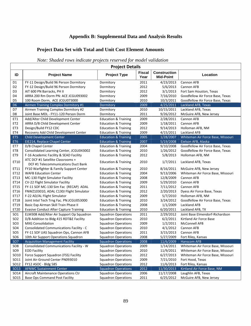
89
Appendix B: Supplemental Data and Analysis Results
Project Data Set with Total and Unit Cost Element Amounts
Note: Shaded rows indicate projects reserved for model validation
Project Details
ID Project Name Project Type Fiscal Year
Construction Mid-Point
Location
D1 FY-11 Design/Build 96 Person Dormitory Dormitory 2011 4/23/2013 Cannon AFB D2 FY-12 Design/Build 96 Person Dormitory Dormitory 2012 5/6/2013 Cannon AFB D3 AIT 600 PN Barracks, PH II Dormitory 2012 3/1/2013 Fort Sam Houston, Texas D4 ARRA 200 Rm Dorm PN: ACE JCGU093002 Dormitory 2009 7/16/2010 Goodfellow Air Force Base, Texas D5 100 Room Dorm, ACE JCGU073000 Dormitory 2010 10/3/2011 Goodfellow Air Force Base, Texas D6 Airmen Training Complex Dormitory #1 Dormitory 2009 4/25/2011 Lackland AFB, Texas D7 Airmen Training Complex Dormitory #2 Dormitory 2010 10/15/2011 Lackland AFB, Texas D8 Joint Base MDL - FY11-120 Person Dorm Dormitory 2011 9/26/2012 McGuire AFB, New Jersey
ET1 Add/Alter Child Development Center Education & Training 2009 2/28/2011 Cannon AFB ET2 ARRA D/B Child Development Center Education & Training 2009 1/18/2011 Cannon AFB ET3 Design/Build FY12 CDC Education & Training 2012 9/14/2013 Holloman AFB, NM ET4 Recovery Add Child Development Center Education & Training 2009 4/15/2011 Lackland AFB ET5 Child Development Center Education & Training 2005 1/28/2007 Whiteman Air Force Base, Missouri ET6 EIE214, Replace Chapel Center Education & Training 2007 5/19/2008 Eielson AFB, Alaska ET7 D/B Chapel Center Education & Training 2004 9/10/2008 Goodfellow Air Force Base, Texas ET8 Consolidated Learning Center, JCGU043002 Education & Training 2010 1/26/2012 Goodfellow Air Force Base, Texas ET9 F-16 Academic Facility & SEAD Facility Education & Training 2012 5/8/2013 Holloman AFB, NM
ET10 ATC DCF #1 Satellite Classrooms + DCF #1 Telecommunications Duct Bank
Education & Training 2010 1/7/2011 Lackland AFB, Texas
ET11 FY10 Warfighter & Family Support Center Education & Training 2010 8/16/2011 McGuire AFB, New Jersey ET12 WAFB Education Center Education & Training 2004 9/13/2006 Whiteman Air Force Base, Missouri ET13 MC-130 Flight Simulator Facility Education & Training 2008 12/8/2009 Cannon AFB ET14 CV-22 Flight Simulator Facility Education & Training 2009 5/29/2010 Cannon AFB ET15 FY-11 SOF MC-130 Sim Fac (RECAP) ADAL Education & Training 2011 7/11/2012 Cannon AFB ET16 FNWZ103010, ADAL C130J Flight Simulator Education & Training 2012 2/20/2013 Dyess Air Force Base, Texas ET17 F-22 AD/AL Flight Simulator Education & Training 2009 5/7/2010 Holloman AFB, NM ET18 Joint Intel Tech Trng Fac. PN:JCGU053000 Education & Training 2010 3/24/2012 Goodfellow Air Force Base, Texas ET19 Basic Exp Airman Skill Train Phase II Education & Training 2008 1/1/2009 Lackland AFB ET20 Evasive Conduct After Capture Training Education & Training 2010 6/20/2011 Lackland AFB, TX
SO1 ELM308 Add/Alter Air Support Op Squadron Squadron Operations 2011 2/29/2012 Joint Base Elmendorf-Richardson SO2 D/B Addition to Bldg 415 RDT&E Facility Squadron Operations 2010 6/2/2011 Kirtland Air Force Base SO3 MXG Consolidation Squadron Operations 2009 1/2/2011 McConnell AFB SO4 Consolidated Communications Facility - C Squadron Operations 2010 4/1/2012 Cannon AFB SO5 FY-11 SOF UAS Squadron Ops, Cannon AFB Squadron Operations 2011 3/15/2013 Cannon AFB SO6 10th Air Support Operations Squadron Squadron Operations 2008 5/27/2009 Fort Riley, Kansas SO7 Acquisition Management Facility Squadron Operations 2008 11/6/2009 Hanscom AFB SO8 Consolidated Communications Facility - W Squadron Operations 2009 1/14/2011 Whiteman Air Force Base, Missouri SO9 EOD Facility Squadron Operations 2010 11/9/2011 Whiteman Air Force Base, Missouri SO10 Force Support Squadron (FSS) Facility Squadron Operations 2012 6/27/2013 Whiteman Air Force Base, Missouri SO11 Joint Air-Ground Center PN093010 Squadron Operations 2009 7/21/2010 Fort Hood, Texas SO12 FY12 ASOC - Bldg 585 Squadron Operations 2012 11/6/2013 Fort Riley, Kansas SO13 AFNWC Sustainment Center Squadron Operations 2012 11/30/2013 Kirtland Air Force Base, NM SO14 Aircraft Maintenance Operations Ctr Squadron Operations 2006 11/17/2008 Laughlin AFB, Texas SO15 Base Ops Command Post Facility Squadron Operations 2011 6/25/2012 McGuire AFB, New Jersey

90
Project Details
ID Project Type
Escala-tion
Factor
Area Cost
Factor
Scope (SM)
AF PA Cost Estimate
Revised AF PA Cost Estimate
Total Actual Cost
D1
Do
rmit
ory
1.0583 1.01 3168.00 $ 14,000,000.00 $ 13,972,000.00 $13,348,830.34
D2 1.0571 1.01 3168.00 $ 15,000,000.00 $ 15,000,000.00 $13,296,383.78
D3 1.0636 0.84 16287.00 $ 46,000,000.00 $ 39,100,000.00 $37,921,845.00
D4 1.1174 0.86 10580.00 $ 28,400,000.00 $ 26,220,228.00 $23,743,643.00
D5 1.0957 0.86 5290.00 $ 14,000,000.00 $ 14,000,000.00 $14,226,979.60
D6 1.1066 0.84 21543.74 $ 75,515,000.00 $ 69,102,000.00 $54,544,986.13
D7 1.0951 0.84 21543.74 $ 77,000,000.00 $ 59,876,098.00 $47,330,700.65
D8 1.0786 1.22 3960.00 $ 18,440,000.00 $ 15,482,000.00 $13,904,784.13
ET1
Edu
cati
on
& T
rain
ing
1.1103 1.01 2379.00 $ 8,000,000.00 $ 7,400,000.00 $7,597,826.14
ET2 1.1131 1.01 2165.00 $ 12,000,000.00 $ 9,574,969.00 $8,775,162.58
ET3 1.0442 0.99 2700.00 $ 11,200,000.00 $ 11,200,000.00 $10,327,370.61
ET4 1.1072 0.84 2787.09 $ 6,000,000.00 $ 6,000,000.00 $6,604,890.78
ET5 1.1042 1.07 2450.00 $ 7,600,000.00 $ 7,600,000.00 $7,685,911.90
ET6 1.0579 2.30 2994.00 $ 14,400,000.00 $ 14,001,108.00 $12,998,688.00
ET7 1.0427 0.86 1680.00 $ 4,300,000.00 $ 4,257,000.00 $4,886,564.00
ET8 1.0902 0.86 2598.00 $ 12,000,000.00 $ 12,000,000.00 $11,277,138.00
ET9 1.0569 0.99 2222.00 $ 10,000,000.00 $ 10,000,000.00 $9,062,924.79
ET10 1.1138 0.84 8074.76 $ 32,000,000.00 $ 28,363,258.00 $27,928,752.97
ET11 1.0989 1.22 1672.00 $ 7,900,000.00 $ 7,900,000.00 $7,042,319.00
ET12 1.1135 1.07 7763.00 $ 13,200,000.00 $ 13,199,374.00 $13,214,270.08
ET13 1.1084 1.01 2200.00 $ 13,287,000.00 $ 12,996,000.00 $8,292,633.94
ET14 1.1154 1.01 2788.00 $ 8,300,000.00 $ 8,280,591.00 $6,043,246.82
ET15 1.0823 1.01 2200.00 $ 13,287,000.00 $ 12,996,000.00 $9,568,809.61
ET16 1.0644 0.89 876.00 $ 4,080,000.00 $ 4,071,000.00 $1,127,205.00
ET17 1.1145 0.99 1022.00 $ 3,150,000.00 $ 3,068,000.00 $3,565,542.23
ET18 1.0875 0.86 4645.00 $ 18,400,000.00 $ 12,698,364.00 $12,749,453.95
ET19 1.0566 0.84 9870.00 $ 14,000,000.00 $ 13,260,000.00 $11,509,243.70
ET20 1.1027 0.84 1487.00 $ 4,879,000.00 $ 4,732,630.00 $5,552,962.00
SO1
Squ
adro
n O
per
atio
ns
1.0886 2.05 1140.00 $ 4,749,000.00 $ 4,740,000.00 $4,202,360.00
SO2 1.1040 0.91 1097.00 $ 5,800,000.00 $ 4,995,734.00 $4,476,007.00
SO3 1.1142 0.92 8088.00 $ 13,100,000.00 $ 12,745,000.00 $13,104,227.36
SO4 1.0871 1.01 5574.00 $ 15,000,000.00 $ 18,071,236.00 $23,522,110.25
SO5 1.0622 1.01 8233.00 $ 39,674,000.00 $ 39,417,000.00 $25,220,848.23
SO6 1.0828 1.05 2980.00 $ 12,515,000.00 $ 12,245,000.00 $11,197,871.31
SO7 1.1071 1.26 3690.01 $ 12,800,000.00 $ 12,790,000.00 $12,236,463.16
SO8 1.1134 1.07 4274.00 $ 11,400,000.00 $ 11,380,000.00 $10,524,677.00
SO9 1.0939 1.07 1505.00 $ 7,400,000.00 $ 7,024,212.00 $7,155,063.58
SO10 1.0520 1.07 1109.00 $ 5,000,000.00 $ 6,373,000.00 $5,969,791.00
SO11 1.1176 0.86 5434.00 $ 10,800,000.00 $ 10,411,000.00 $8,671,894.13
SO12 1.0383 1.05 4000.00 $ 7,600,000.00 $ 7,600,000.00 $5,791,035.00
SO13 1.0356 0.91 5310.00 $ 25,000,000.00 $ 23,900,000.00 $24,355,245.36
SO14 1.0485 0.89 1869.00 $ 7,900,000.00 $ 7,820,846.00 $7,972,997.77
SO15 1.0831 1.22 2200.00 $ 8,000,000.00 $ 7,951,000.00 $6,913,267.00

91
Cost Summary
ID Project Type
General Requirements
Demolition Finishes Foundations Communi-
cations Pavements
D1
Do
rmit
ory
$1,139,429.00 $0.00 $1,999,104.74 $506,250.00 $109,815.00 $405,268.00
D2 $937,851.47 $0.00 $2,176,998.23 $506,250.00 $109,759.00 $395,729.00
D3 $3,331,509.00 $3,186,598.00 $3,268,561.00 $1,866,000.00 $1,120,000.00 $2,479,001.00
D4 $2,478,119.00 $0.00 $4,666,315.00 $2,437,406.00 $295,929.00 $797,620.00
D5 $959,993.10 $26,069.00 $1,955,254.00 $1,894,636.50 $812,012.00 $573,686.00
D6 $7,164,159.26 $183,948.00 $5,492,013.00 $4,677,628.00 $1,575,025.00 $1,422,127.00
D7 $6,428,998.00 $401,859.00 $4,186,096.82 $4,219,867.64 $1,770,342.10 $2,894,436.35
D8 $1,391,162.30 $50,000.00 $2,697,500.00 $744,716.45 $748,830.18 $542,715.00
ET1
Edu
cati
on
& T
rain
ing
$1,376,135.30 $191,555.00 $601,715.62 $366,445.00 $139,067.09 $454,865.86
ET2 $1,589,048.58 $115,316.00 $1,491,087.00 $482,620.00 $313,381.00 $471,187.00
ET3 $1,568,351.46 $87,509.24 $1,893,177.00 $540,000.00 $225,000.00 $641,175.00
ET4 $890,767.00 $67,057.00 $1,482,686.00 $172,290.00 $308,595.00 $268,648.00
ET5 $650,207.00 $403,593.90 $1,075,066.00 $338,373.00 $109,020.00 $525,211.00
ET6 $1,664,538.00 $0.00 $2,451,845.00 $1,183,778.00 $650,614.00 $381,730.00
ET7 $728,899.00 $46,462.00 $906,243.00 $485,000.00 $179,500.00 $45,000.00
ET8 $1,085,938.60 $347,060.00 $1,822,148.40 $674,380.85 $883,506.15 $670,609.00
ET9 $1,063,737.10 $145,512.00 $1,420,631.69 $730,359.00 $664,586.00 $571,148.00
ET10 $1,496,034.91 $85,983.09 $2,890,037.02 $1,904,368.35 $1,300,143.04 $1,258,866.98
ET11 $733,404.00 $216,300.00 $1,250,747.00 $412,550.00 $49,000.00 $277,650.00
ET12 $1,108,231.48 $92,500.00 $2,660,497.00 $1,223,530.00 $69,000.00 $290,800.00
ET13 $372,882.91 $74,407.00 $1,292,351.37 $246,021.00 $629,716.00 $928,440.00
ET14 $393,665.89 $15,000.00 $937,808.00 $218,642.00 $631,384.00 $737,098.00
ET15 $466,567.77 $109,458.04 $1,257,480.86 $579,078.20 $786,753.53 $264,684.28
ET16 $91,276.00 $18,363.00 $177,585.00 $121,594.00 $42,752.00 $61,032.00
ET17 $287,592.30 $46,455.72 $807,967.08 $168,304.45 $229,546.75 $82,417.11
ET18 $121,394.08 $82,353.00 $2,294,947.19 $1,874,997.33 $541,666.27 $737,839.00
ET19 $733,346.00 $55,544.00 $1,028,825.00 $956,658.00 $1,245,872.00 $1,313,332.00
ET20 $553,822.00 $0.00 $522,691.00 $331,575.00 $557,966.00 $86,069.00
SO1
Squ
adro
n O
per
atio
ns
$732,392.00 $121,948.25 $187,580.74 $13,400.74 $168,623.03 $164,760.74
SO2 $492,227.00 $78,249.00 $732,800.00 $77,051.00 $544,303.00 $301,193.00
SO3 $1,324,824.38 $913,981.00 $4,737,322.00 $345,000.00 $139,068.00 $291,949.00
SO4 $2,877,016.49 $323,413.70 $2,041,110.71 $891,747.62 $3,126,154.18 $1,556,210.00
SO5 $1,643,407.86 $205,000.00 $2,674,299.12 $2,298,478.00 $2,269,945.15 $1,791,400.00
SO6 $991,417.00 $0.00 $1,773,599.31 $1,161,696.00 $317,666.00 $726,469.00
SO7 $2,383,825.00 $10,000.00 $1,887,000.00 $0.00 $111,200.00 $815,000.00
SO8 $1,198,358.50 $323,828.00 $954,546.00 $1,273,802.00 $457,332.00 $472,901.00
SO9 $1,456,378.58 $253,601.00 $1,057,152.00 $308,000.00 $236,179.00 $348,048.00
SO10 $581,937.27 $22,329.68 $781,990.77 $423,382.75 $566,448.90 $249,807.94
SO11 $1,644,235.66 $17,874.16 $1,408,956.53 $476,313.44 $61,764.00 $480,995.11
SO12 $735,511.00 $8,957.00 $385,065.00 $940,000.00 $243,500.00 $181,000.00
SO13 $2,819,040.00 $144,977.00 $1,630,000.00 $1,271,000.00 $5,748,879.11 $484,681.00
SO14 $953,682.00 $431,235.49 $1,111,103.00 $198,357.00 $122,107.00 $725,758.28
SO15 $171,241.00 $94,000.00 $1,713,000.00 $408,759.00 $624,000.00 $220,399.00
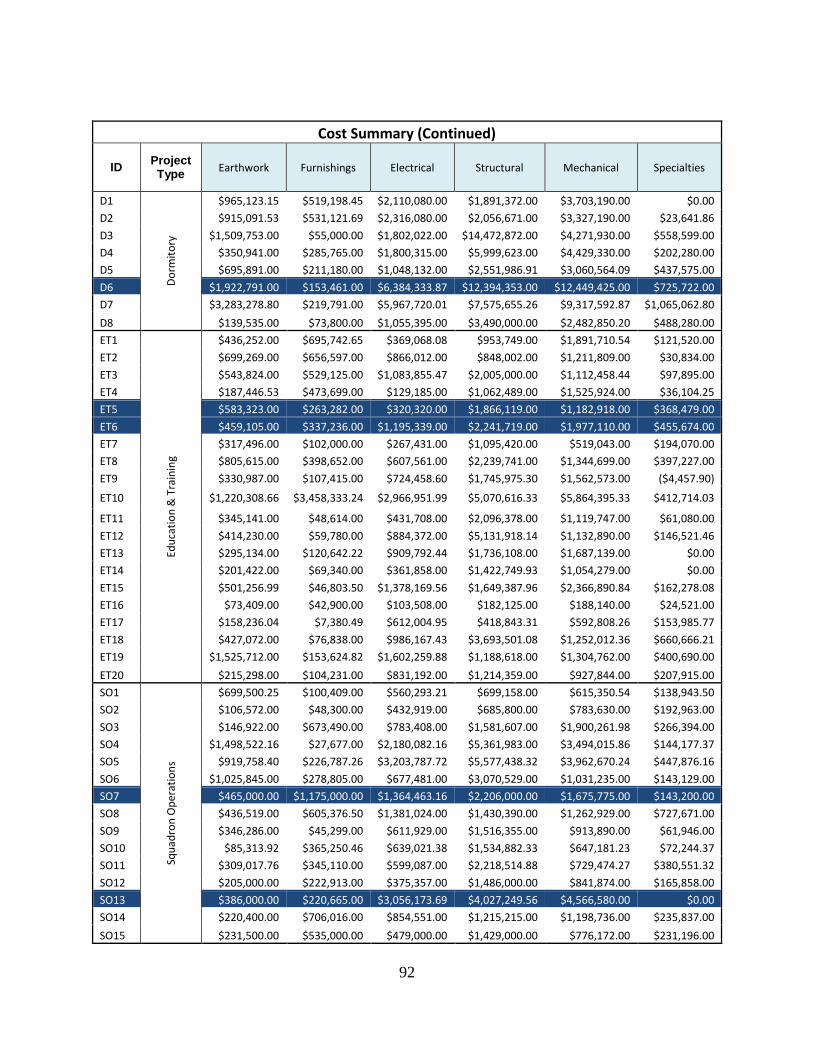
92
Cost Summary (Continued)
ID Project Type
Earthwork Furnishings Electrical Structural Mechanical Specialties
D1
Do
rmit
ory
$965,123.15 $519,198.45 $2,110,080.00 $1,891,372.00 $3,703,190.00 $0.00
D2 $915,091.53 $531,121.69 $2,316,080.00 $2,056,671.00 $3,327,190.00 $23,641.86
D3 $1,509,753.00 $55,000.00 $1,802,022.00 $14,472,872.00 $4,271,930.00 $558,599.00
D4 $350,941.00 $285,765.00 $1,800,315.00 $5,999,623.00 $4,429,330.00 $202,280.00
D5 $695,891.00 $211,180.00 $1,048,132.00 $2,551,986.91 $3,060,564.09 $437,575.00
D6 $1,922,791.00 $153,461.00 $6,384,333.87 $12,394,353.00 $12,449,425.00 $725,722.00
D7 $3,283,278.80 $219,791.00 $5,967,720.01 $7,575,655.26 $9,317,592.87 $1,065,062.80
D8 $139,535.00 $73,800.00 $1,055,395.00 $3,490,000.00 $2,482,850.20 $488,280.00
ET1
Edu
cati
on
& T
rain
ing
$436,252.00 $695,742.65 $369,068.08 $953,749.00 $1,891,710.54 $121,520.00
ET2 $699,269.00 $656,597.00 $866,012.00 $848,002.00 $1,211,809.00 $30,834.00
ET3 $543,824.00 $529,125.00 $1,083,855.47 $2,005,000.00 $1,112,458.44 $97,895.00
ET4 $187,446.53 $473,699.00 $129,185.00 $1,062,489.00 $1,525,924.00 $36,104.25
ET5 $583,323.00 $263,282.00 $320,320.00 $1,866,119.00 $1,182,918.00 $368,479.00
ET6 $459,105.00 $337,236.00 $1,195,339.00 $2,241,719.00 $1,977,110.00 $455,674.00
ET7 $317,496.00 $102,000.00 $267,431.00 $1,095,420.00 $519,043.00 $194,070.00
ET8 $805,615.00 $398,652.00 $607,561.00 $2,239,741.00 $1,344,699.00 $397,227.00
ET9 $330,987.00 $107,415.00 $724,458.60 $1,745,975.30 $1,562,573.00 ($4,457.90)
ET10 $1,220,308.66 $3,458,333.24 $2,966,951.99 $5,070,616.33 $5,864,395.33 $412,714.03
ET11 $345,141.00 $48,614.00 $431,708.00 $2,096,378.00 $1,119,747.00 $61,080.00
ET12 $414,230.00 $59,780.00 $884,372.00 $5,131,918.14 $1,132,890.00 $146,521.46
ET13 $295,134.00 $120,642.22 $909,792.44 $1,736,108.00 $1,687,139.00 $0.00
ET14 $201,422.00 $69,340.00 $361,858.00 $1,422,749.93 $1,054,279.00 $0.00
ET15 $501,256.99 $46,803.50 $1,378,169.56 $1,649,387.96 $2,366,890.84 $162,278.08
ET16 $73,409.00 $42,900.00 $103,508.00 $182,125.00 $188,140.00 $24,521.00
ET17 $158,236.04 $7,380.49 $612,004.95 $418,843.31 $592,808.26 $153,985.77
ET18 $427,072.00 $76,838.00 $986,167.43 $3,693,501.08 $1,252,012.36 $660,666.21
ET19 $1,525,712.00 $153,624.82 $1,602,259.88 $1,188,618.00 $1,304,762.00 $400,690.00
ET20 $215,298.00 $104,231.00 $831,192.00 $1,214,359.00 $927,844.00 $207,915.00
SO1
Squ
adro
n O
per
atio
ns
$699,500.25 $100,409.00 $560,293.21 $699,158.00 $615,350.54 $138,943.50
SO2 $106,572.00 $48,300.00 $432,919.00 $685,800.00 $783,630.00 $192,963.00
SO3 $146,922.00 $673,490.00 $783,408.00 $1,581,607.00 $1,900,261.98 $266,394.00
SO4 $1,498,522.16 $27,677.00 $2,180,082.16 $5,361,983.00 $3,494,015.86 $144,177.37
SO5 $919,758.40 $226,787.26 $3,203,787.72 $5,577,438.32 $3,962,670.24 $447,876.16
SO6 $1,025,845.00 $278,805.00 $677,481.00 $3,070,529.00 $1,031,235.00 $143,129.00
SO7 $465,000.00 $1,175,000.00 $1,364,463.16 $2,206,000.00 $1,675,775.00 $143,200.00
SO8 $436,519.00 $605,376.50 $1,381,024.00 $1,430,390.00 $1,262,929.00 $727,671.00
SO9 $346,286.00 $45,299.00 $611,929.00 $1,516,355.00 $913,890.00 $61,946.00
SO10 $85,313.92 $365,250.46 $639,021.38 $1,534,882.33 $647,181.23 $72,244.37
SO11 $309,017.76 $345,110.00 $599,087.00 $2,218,514.88 $729,474.27 $380,551.32
SO12 $205,000.00 $222,913.00 $375,357.00 $1,486,000.00 $841,874.00 $165,858.00
SO13 $386,000.00 $220,665.00 $3,056,173.69 $4,027,249.56 $4,566,580.00 $0.00
SO14 $220,400.00 $706,016.00 $854,551.00 $1,215,215.00 $1,198,736.00 $235,837.00
SO15 $231,500.00 $535,000.00 $479,000.00 $1,429,000.00 $776,172.00 $231,196.00
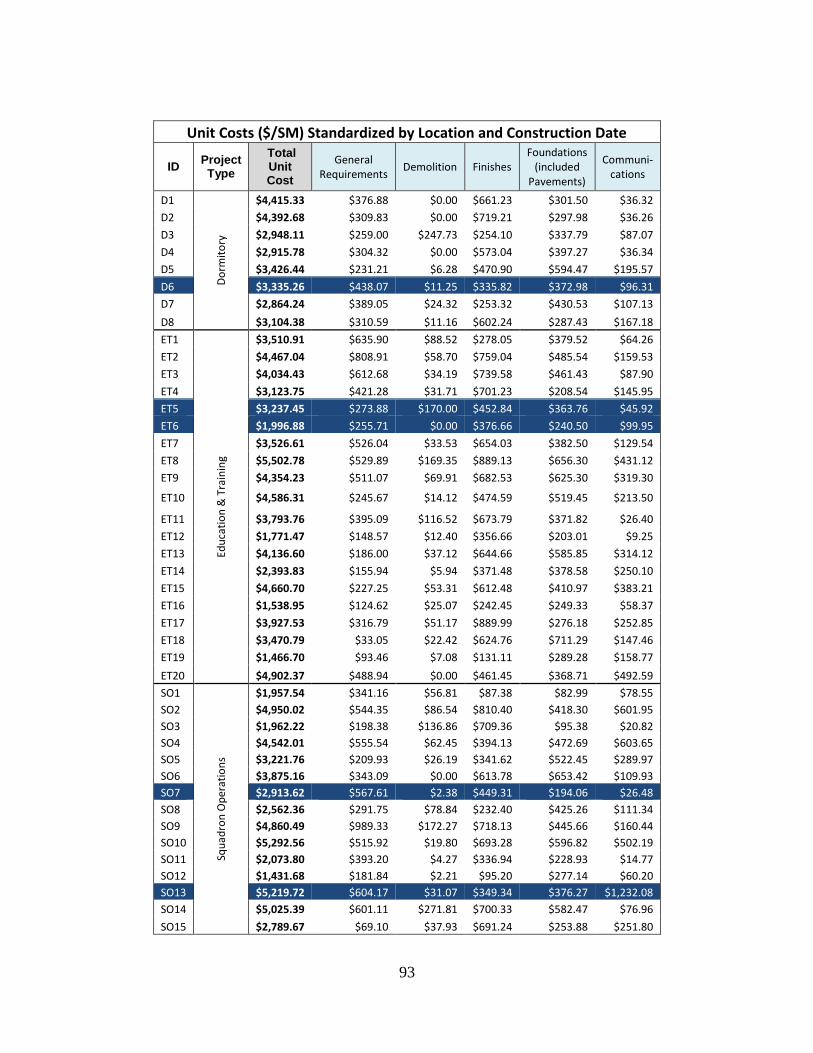
93
Unit Costs ($/SM) Standardized by Location and Construction Date
ID Project Type
Total Unit Cost
General Requirements
Demolition Finishes Foundations
(included Pavements)
Communi-cations
D1
Do
rmit
ory
$4,415.33 $376.88 $0.00 $661.23 $301.50 $36.32
D2 $4,392.68 $309.83 $0.00 $719.21 $297.98 $36.26
D3 $2,948.11 $259.00 $247.73 $254.10 $337.79 $87.07
D4 $2,915.78 $304.32 $0.00 $573.04 $397.27 $36.34
D5 $3,426.44 $231.21 $6.28 $470.90 $594.47 $195.57
D6 $3,335.26 $438.07 $11.25 $335.82 $372.98 $96.31
D7 $2,864.24 $389.05 $24.32 $253.32 $430.53 $107.13
D8 $3,104.38 $310.59 $11.16 $602.24 $287.43 $167.18
ET1
Edu
cati
on
& T
rain
ing
$3,510.91 $635.90 $88.52 $278.05 $379.52 $64.26
ET2 $4,467.04 $808.91 $58.70 $759.04 $485.54 $159.53
ET3 $4,034.43 $612.68 $34.19 $739.58 $461.43 $87.90
ET4 $3,123.75 $421.28 $31.71 $701.23 $208.54 $145.95
ET5 $3,237.45 $273.88 $170.00 $452.84 $363.76 $45.92
ET6 $1,996.88 $255.71 $0.00 $376.66 $240.50 $99.95
ET7 $3,526.61 $526.04 $33.53 $654.03 $382.50 $129.54
ET8 $5,502.78 $529.89 $169.35 $889.13 $656.30 $431.12
ET9 $4,354.23 $511.07 $69.91 $682.53 $625.30 $319.30
ET10 $4,586.31 $245.67 $14.12 $474.59 $519.45 $213.50
ET11 $3,793.76 $395.09 $116.52 $673.79 $371.82 $26.40
ET12 $1,771.47 $148.57 $12.40 $356.66 $203.01 $9.25
ET13 $4,136.60 $186.00 $37.12 $644.66 $585.85 $314.12
ET14 $2,393.83 $155.94 $5.94 $371.48 $378.58 $250.10
ET15 $4,660.70 $227.25 $53.31 $612.48 $410.97 $383.21
ET16 $1,538.95 $124.62 $25.07 $242.45 $249.33 $58.37
ET17 $3,927.53 $316.79 $51.17 $889.99 $276.18 $252.85
ET18 $3,470.79 $33.05 $22.42 $624.76 $711.29 $147.46
ET19 $1,466.70 $93.46 $7.08 $131.11 $289.28 $158.77
ET20 $4,902.37 $488.94 $0.00 $461.45 $368.71 $492.59
SO1
Squ
adro
n O
per
atio
ns
$1,957.54 $341.16 $56.81 $87.38 $82.99 $78.55
SO2 $4,950.02 $544.35 $86.54 $810.40 $418.30 $601.95
SO3 $1,962.22 $198.38 $136.86 $709.36 $95.38 $20.82
SO4 $4,542.01 $555.54 $62.45 $394.13 $472.69 $603.65
SO5 $3,221.76 $209.93 $26.19 $341.62 $522.45 $289.97
SO6 $3,875.16 $343.09 $0.00 $613.78 $653.42 $109.93
SO7 $2,913.62 $567.61 $2.38 $449.31 $194.06 $26.48
SO8 $2,562.36 $291.75 $78.84 $232.40 $425.26 $111.34
SO9 $4,860.49 $989.33 $172.27 $718.13 $445.66 $160.44
SO10 $5,292.56 $515.92 $19.80 $693.28 $596.82 $502.19
SO11 $2,073.80 $393.20 $4.27 $336.94 $228.93 $14.77
SO12 $1,431.68 $181.84 $2.21 $95.20 $277.14 $60.20
SO13 $5,219.72 $604.17 $31.07 $349.34 $376.27 $1,232.08
SO14 $5,025.39 $601.11 $271.81 $700.33 $582.47 $76.96
SO15 $2,789.67 $69.10 $37.93 $691.24 $253.88 $251.80

94
Unit Costs ($/SM) (Continued)
ID Project Type
Earthwork Furnishings Electrical Structural Mechanical Specialties
D1
Do
rmit
ory
$319.23 $171.73 $697.94 $625.60 $1,224.89 $0.00
D2 $302.32 $175.46 $765.16 $679.46 $1,099.19 $7.81
D3 $117.37 $4.28 $140.09 $1,125.14 $332.11 $43.43
D4 $43.10 $35.09 $221.08 $736.77 $543.93 $24.84
D5 $167.60 $50.86 $252.43 $614.62 $737.11 $105.39
D6 $117.57 $9.38 $390.38 $757.88 $761.24 $44.38
D7 $198.69 $13.30 $361.14 $458.44 $563.86 $64.45
D8 $31.15 $16.48 $235.63 $779.18 $554.32 $109.01
ET1
Edu
cati
on
& T
rain
ing
$201.59 $321.50 $170.54 $440.72 $874.15 $56.15
ET2 $355.97 $334.24 $440.85 $431.68 $616.88 $15.70
ET3 $212.45 $206.70 $423.41 $783.26 $434.59 $38.24
ET4 $88.65 $224.03 $61.10 $502.50 $721.68 $17.08
ET5 $245.71 $110.90 $134.92 $786.04 $498.27 $155.21
ET6 $70.53 $51.81 $183.63 $344.38 $303.73 $70.00
ET7 $229.14 $73.61 $193.00 $790.56 $374.59 $140.06
ET8 $393.11 $194.53 $296.47 $1,092.90 $656.16 $193.83
ET9 $159.02 $51.61 $348.06 $838.84 $750.73 ($2.14)
ET10 $200.39 $567.91 $487.22 $832.67 $963.02 $67.77
ET11 $185.93 $26.19 $232.56 $1,129.34 $603.22 $32.90
ET12 $55.53 $8.01 $118.56 $687.97 $151.87 $19.64
ET13 $147.22 $60.18 $453.83 $866.02 $841.59 $0.00
ET14 $79.79 $27.47 $143.34 $563.58 $417.62 $0.00
ET15 $244.15 $22.80 $671.27 $803.37 $1,152.85 $79.04
ET16 $100.22 $58.57 $141.32 $248.65 $256.86 $33.48
ET17 $174.30 $8.13 $674.14 $461.37 $652.99 $169.62
ET18 $116.26 $20.92 $268.47 $1,005.48 $340.84 $179.85
ET19 $194.43 $19.58 $204.19 $151.47 $166.27 $51.06
ET20 $190.07 $92.02 $733.81 $1,072.08 $819.14 $183.56
SO1
Squ
adro
n O
per
atio
ns
$325.84 $46.77 $261.00 $325.68 $286.64 $64.72
SO2 $117.86 $53.42 $478.77 $758.43 $866.62 $213.40
SO3 $22.00 $100.85 $117.31 $236.83 $284.54 $39.89
SO4 $289.36 $5.34 $420.96 $1,035.37 $674.68 $27.84
SO5 $117.49 $28.97 $409.26 $712.47 $506.20 $57.21
SO6 $355.01 $96.48 $234.45 $1,062.60 $356.87 $49.53
SO7 $110.72 $279.78 $324.89 $525.27 $399.02 $34.10
SO8 $106.28 $147.39 $336.23 $348.25 $307.47 $177.16
SO9 $235.23 $30.77 $415.69 $1,030.07 $620.81 $42.08
SO10 $75.64 $323.82 $566.53 $1,360.76 $573.76 $64.05
SO11 $73.90 $82.53 $143.27 $530.54 $174.45 $91.01
SO12 $50.68 $55.11 $92.80 $367.37 $208.13 $41.00
SO13 $82.73 $47.29 $654.99 $863.10 $978.69 $0.00
SO14 $138.92 $445.00 $538.62 $765.95 $755.57 $148.65
SO15 $93.42 $215.89 $193.29 $576.64 $313.20 $93.29
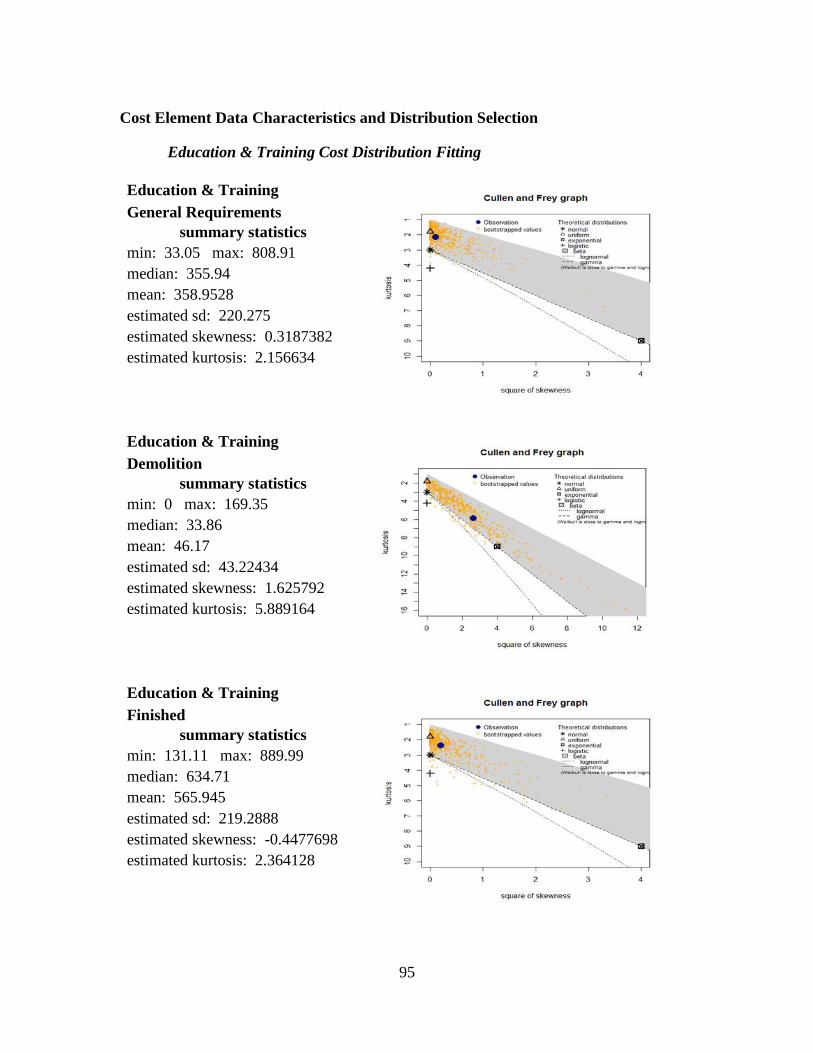
95
Cost Element Data Characteristics and Distribution Selection
Education & Training Cost Distribution Fitting
Education & Training
General Requirements
summary statistics
min: 33.05 max: 808.91
median: 355.94
mean: 358.9528
estimated sd: 220.275
estimated skewness: 0.3187382
estimated kurtosis: 2.156634
Education & Training
Demolition
summary statistics
min: 0 max: 169.35
median: 33.86
mean: 46.17
estimated sd: 43.22434
estimated skewness: 1.625792
estimated kurtosis: 5.889164
Education & Training
Finished
summary statistics
min: 131.11 max: 889.99
median: 634.71
mean: 565.945
estimated sd: 219.2888
estimated skewness: -0.4477698
estimated kurtosis: 2.364128
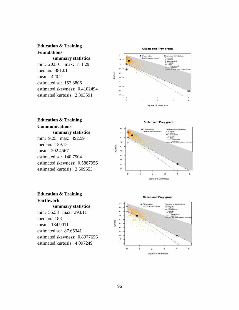
96
Education & Training
Foundations
summary statistics
min: 203.01 max: 711.29
median: 381.01
mean: 420.2
estimated sd: 152.3806
estimated skewness: 0.4102494
estimated kurtosis: 2.303591
Education & Training
Communications
summary statistics
min: 9.25 max: 492.59
median: 159.15
mean: 202.4567
estimated sd: 140.7504
estimated skewness: 0.5887956
estimated kurtosis: 2.509553
Education & Training
Earthwork
summary statistics
min: 55.53 max: 393.11
median: 188
mean: 184.9011
estimated sd: 87.65341
estimated skewness: 0.8977656
estimated kurtosis: 4.097249

97
Education & Training
Furnishings
summary statistics
min: 8.01 max: 567.91
median: 59.375
mean: 128.7778
estimated sd: 152.6941
estimated skewness: 1.699039
estimated kurtosis: 5.805655
Education & Training
Electric
summary statistics
min: 61.1 max: 733.81
median: 282.47
mean: 336.7856
estimated sd: 205.8566
estimated skewness: 0.6654147
estimated kurtosis: 2.362561
Education & Training
Structural
summary statistics
min: 151.47 max: 1129.34
median: 786.91
mean: 705.6922
estimated sd: 288.8792
estimated skewness: -0.3018995
estimated kurtosis: 2.233272
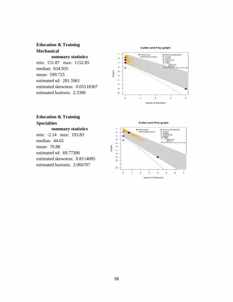
98
Education & Training
Mechanical
summary statistics
min: 151.87 max: 1152.85
median: 634.935
mean: 599.725
estimated sd: 281.5961
estimated skewness: 0.05118367
estimated kurtosis: 2.3396
Education & Training
Specialties
summary statistics
min: -2.14 max: 193.83
median: 44.65
mean: 70.88
estimated sd: 69.77306
estimated skewness: 0.8114085
estimated kurtosis: 2.066707

99
Dormitory Cost Distribution Fitting
Dormitories
General Requirements
summary statistics
min: 231.21 max: 389.05
median: 309.83
mean: 311.5543
estimated sd: 57.0766
estimated skewness: 0.1003973
estimated kurtosis: 2.154556
Dormitories
Demolition
summary statistics
min: 0 max: 247.73
median: 6.28
mean: 41.35571
estimated sd: 91.42714
estimated skewness: 2.595725
estimated kurtosis: 9.789977
Dormitories
Finished
summary statistics
min: 253.32 max: 719.21
median: 573.04
mean: 504.8629
estimated sd: 187.8985
estimated skewness: -0.5913273
estimated kurtosis: 1.63557

100
Dormitories
Foundations
summary statistics
min: 287.43 max: 594.47
median: 337.79
mean: 378.1386
estimated sd: 109.594
estimated skewness: 1.506329
estimated kurtosis: 5.182505
Dormitories
Communications
summary statistics
min: 36.26 max: 195.57
median: 87.07
mean: 95.12429
estimated sd: 65.66191
estimated skewness: 0.6414909
estimated kurtosis: 1.734263
Dormitories
Earthwork
summary statistics
min: 31.15 max: 319.23
median: 167.6
mean: 168.4943
estimated sd: 114.5601
estimated skewness: 0.1789532
estimated kurtosis: 1.522481

101
Dormitories
Furnishings
summary statistics
min: 4.28 max: 175.46
median: 35.09
mean: 66.74286
estimated sd: 74.58774
estimated skewness: 1.058897
estimated kurtosis: 2.003004
Dormitories
Electric
summary statistics
min: 140.09 max: 765.16
median: 252.43
mean: 381.9243
estimated sd: 248.2247
estimated skewness: 0.9798782
estimated kurtosis: 2.071009
Dormitories
Structural
summary statistics
min: 458.44 max: 1125.14
median: 679.46
mean: 717.03
estimated sd: 207.3377
estimated skewness: 1.283707
estimated kurtosis: 5.783758
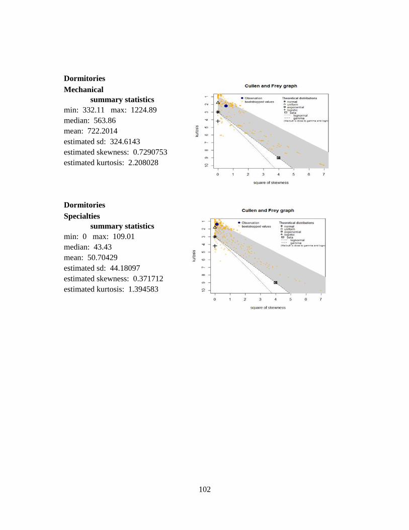
102
Dormitories
Mechanical
summary statistics
min: 332.11 max: 1224.89
median: 563.86
mean: 722.2014
estimated sd: 324.6143
estimated skewness: 0.7290753
estimated kurtosis: 2.208028
Dormitories
Specialties
summary statistics
min: 0 max: 109.01
median: 43.43
mean: 50.70429
estimated sd: 44.18097
estimated skewness: 0.371712
estimated kurtosis: 1.394583

103
Squadron Operations Cost Fitting
Squadron Operations
General Requirements
summary statistics
min: 69.1 max: 989.33
median: 343.09
mean: 402.6692
estimated sd: 241.2572
estimated skewness: 1.067544
estimated kurtosis: 4.736978
Squadron Operations
Demolition
summary statistics
min: 0 max: 271.81
median: 56.81
mean: 73.53692
estimated sd: 79.24672
estimated skewness: 1.505535
estimated kurtosis: 5.190027
Squadron Operations
Finished
summary statistics
min: 87.38 max: 810.4
median: 613.78
mean: 494.1685
estimated sd: 255.4303
estimated skewness: -0.4630197
estimated kurtosis: 1.612724

104
Squadron Operations
Foundations
summary statistics
min: 82.99 max: 653.42
median: 425.26
mean: 388.8762
estimated sd: 186.4094
estimated skewness: -0.3627713
estimated kurtosis: 2.0268
Squadron Operations
Communications
summary statistics
min: 14.77 max: 603.65
median: 111.34
mean: 221.7362
estimated sd: 214.833
estimated skewness: 1.022463
estimated kurtosis: 2.549006
Squadron Operations
Earthwork
summary statistics
min: 22 max: 355.01
median: 117.49
mean: 153.9715
estimated sd: 109.6675
estimated skewness: 0.8509338
estimated kurtosis: 2.317123

105
Squadron Operations
Furnishings
summary statistics
min: 5.34 max: 445
median: 82.53
mean: 125.5646
estimated sd: 129.8832
estimated skewness: 1.632063
estimated kurtosis: 5.126521
Squadron Operations
Electric
summary statistics
min: 92.8 max: 566.53
median: 336.23
mean: 323.7062
estimated sd: 161.2382
estimated skewness: 0.003404834
estimated kurtosis: 1.620349
Squadron Operations
Structural
summary statistics
min: 236.83 max: 1360.76
median: 712.47
mean: 700.8431
estimated sd: 345.2485
estimated skewness: 0.4016622
estimated kurtosis: 2.237809
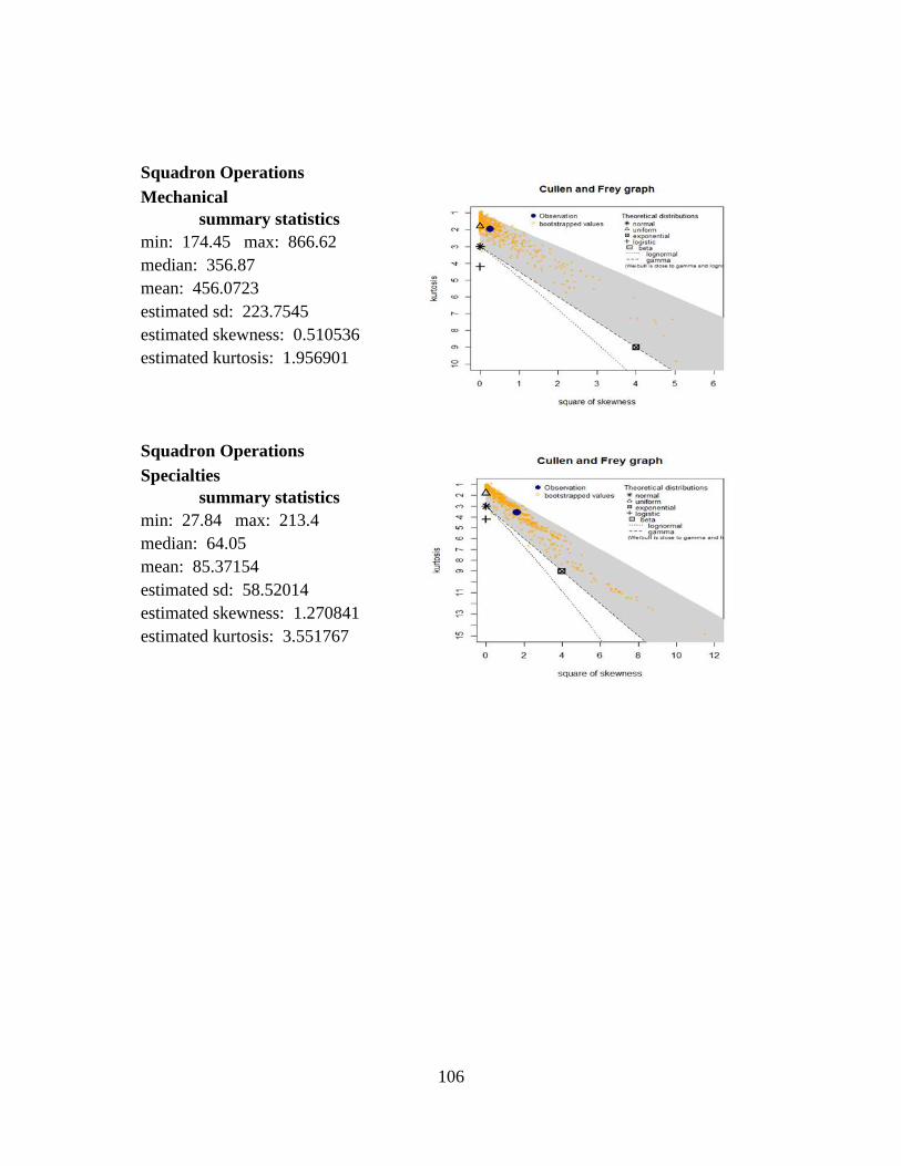
106
Squadron Operations
Mechanical
summary statistics
min: 174.45 max: 866.62
median: 356.87
mean: 456.0723
estimated sd: 223.7545
estimated skewness: 0.510536
estimated kurtosis: 1.956901
Squadron Operations
Specialties
summary statistics
min: 27.84 max: 213.4
median: 64.05
mean: 85.37154
estimated sd: 58.52014
estimated skewness: 1.270841
estimated kurtosis: 3.551767
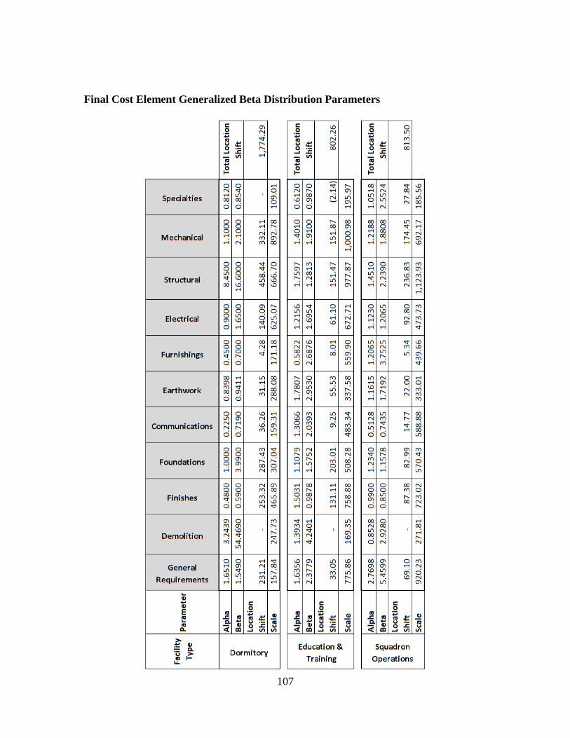
107
Final Cost Element Generalized Beta Distribution Parameters
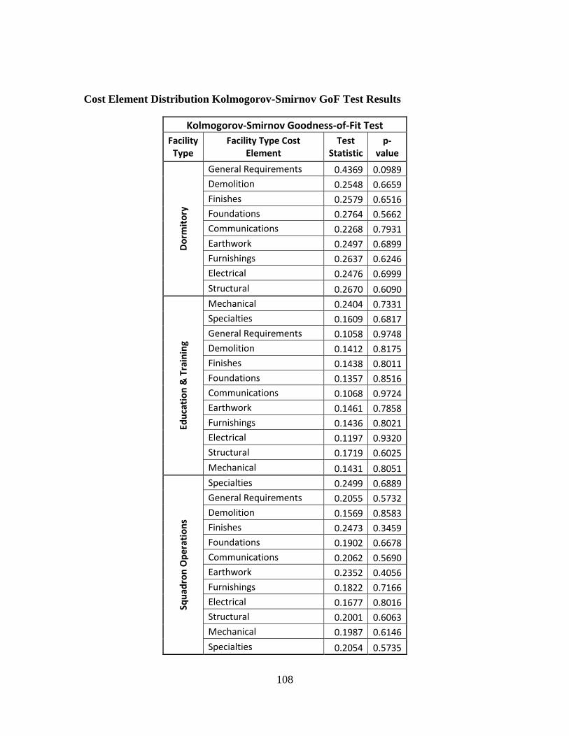
108
Cost Element Distribution Kolmogorov-Smirnov GoF Test Results
Kolmogorov-Smirnov Goodness-of-Fit Test
Facility Type
Facility Type Cost Element
Test Statistic
p-value
Do
rmit
ory
General Requirements 0.4369 0.0989
Demolition 0.2548 0.6659
Finishes 0.2579 0.6516
Foundations 0.2764 0.5662
Communications 0.2268 0.7931
Earthwork 0.2497 0.6899
Furnishings 0.2637 0.6246
Electrical 0.2476 0.6999
Structural 0.2670 0.6090
Edu
cati
on
& T
rain
ing
Mechanical 0.2404 0.7331
Specialties 0.1609 0.6817
General Requirements 0.1058 0.9748
Demolition 0.1412 0.8175
Finishes 0.1438 0.8011
Foundations 0.1357 0.8516
Communications 0.1068 0.9724
Earthwork 0.1461 0.7858
Furnishings 0.1436 0.8021
Electrical 0.1197 0.9320
Structural 0.1719 0.6025
Mechanical 0.1431 0.8051
Squ
adro
n O
per
atio
ns
Specialties 0.2499 0.6889
General Requirements 0.2055 0.5732
Demolition 0.1569 0.8583
Finishes 0.2473 0.3459
Foundations 0.1902 0.6678
Communications 0.2062 0.5690
Earthwork 0.2352 0.4056
Furnishings 0.1822 0.7166
Electrical 0.1677 0.8016
Structural 0.2001 0.6063
Mechanical 0.1987 0.6146
Specialties 0.2054 0.5735

109
Cost Element Correlation Matrices by Facility Type
Dormitory Facilities Initial Infeasible Correlation Matrix
Gen
eral
Req
uir
emen
ts
Dem
olit
ion
Fin
ish
es
Fou
nd
atio
ns
Co
mm
un
i-
cati
on
s
Eart
hw
ork
Furn
ish
ings
Elec
tric
al
Stru
ctu
ral
Mec
han
ical
Spec
ialt
ies
General Requirements
1 -0.037 0.107 -0.321 -0.250 0.357 0.000 0.500 -0.357 0.357 -0.179
Demolition -0.037 1 -0.778 0.185 0.593 -0.371 -0.889 -0.519 0.185 -0.593 0.630
Finishes 0.107 -0.778 1 -0.714 -0.607 0.286 0.821 0.536 0.179 0.571 -0.500
Foundations -0.321 0.185 -0.714 1 0.429 0.071 -0.214 -0.179 -0.571 -0.107 0.179
Communi-cations
-0.250 0.593 -0.607 0.429 1 -0.536 -0.500 -0.429 -0.143 -0.321 0.929
Earthwork 0.357 -0.371 0.286 0.071 -0.536 1 0.571 0.821 -0.607 0.821 -0.679
Furnishings 0.000 -0.889 0.821 -0.214 -0.500 0.571 1 0.750 -0.321 0.821 -0.536
Electrical 0.500 -0.519 0.536 -0.179 -0.429 0.821 0.750 1 -0.643 0.929 -0.429
Structural -0.357 0.185 0.179 -0.571 -0.143 -0.607 -0.321 -0.643 1 -0.643 0.036
Mechanical 0.357 -0.593 0.571 -0.107 -0.321 0.821 0.821 0.929 -0.643 1 -0.429
Specialties -0.179 0.630 -0.500 0.179 0.929 -0.679 -0.536 -0.429 0.036 -0.429 1
Dormitory Facilities Transformed Nearest Positive Definite Matrix
Gen
eral
Req
uir
emen
ts
Dem
olit
ion
Fin
ish
es
Fou
nd
atio
ns
Co
mm
un
i-
cati
on
s
Eart
hw
ork
Furn
ish
ings
Elec
tric
al
Stru
ctu
ral
Mec
han
ical
Spec
ialt
ies
General Requirements
1 -0.037 0.107 -0.321 -0.250 0.357 0.000 0.500 -0.357 0.357 -0.179
Demolition -0.037 1 -0.778 0.185 0.593 -0.371 -0.889 -0.519 0.185 -0.593 0.630
Finishes 0.107 -0.778 1 -0.714 -0.607 0.286 0.821 0.536 0.179 0.571 -0.500
Foundations -0.321 0.185 -0.714 1 0.429 0.071 -0.214 -0.179 -0.571 -0.107 0.179
Communi-cations
-0.250 0.593 -0.607 0.429 1 -0.536 -0.500 -0.429 -0.143 -0.321 0.929
Earthwork 0.357 -0.371 0.286 0.071 -0.536 1 0.571 0.821 -0.607 0.821 -0.679
Furnishings 0.000 -0.889 0.821 -0.214 -0.500 0.571 1 0.750 -0.321 0.821 -0.536
Electrical 0.500 -0.519 0.536 -0.179 -0.429 0.821 0.750 1 -0.643 0.929 -0.429
Structural -0.357 0.185 0.179 -0.571 -0.143 -0.607 -0.321 -0.643 1 -0.643 0.036
Mechanical 0.357 -0.593 0.571 -0.107 -0.321 0.821 0.821 0.929 -0.643 1 -0.429
Specialties -0.179 0.630 -0.500 0.179 0.929 -0.679 -0.536 -0.429 0.036 -0.429 1
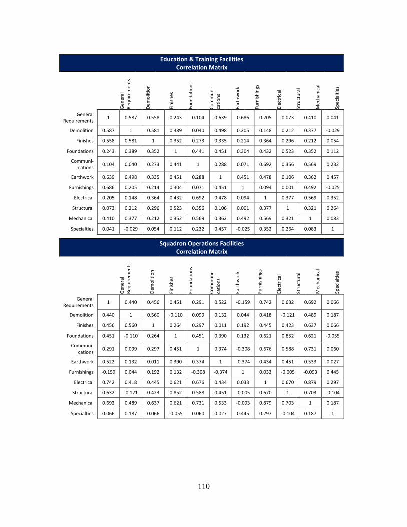
110
Education & Training Facilities Correlation Matrix
Gen
eral
R
equ
irem
ents
Dem
olit
ion
Fin
ish
es
Fou
nd
atio
ns
Co
mm
un
i-
cati
on
s
Eart
hw
ork
Furn
ish
ings
Elec
tric
al
Stru
ctu
ral
Mec
han
ical
Spec
ialt
ies
General Requirements
1 0.587 0.558 0.243 0.104 0.639 0.686 0.205 0.073 0.410 0.041
Demolition 0.587 1 0.581 0.389 0.040 0.498 0.205 0.148 0.212 0.377 -0.029
Finishes 0.558 0.581 1 0.352 0.273 0.335 0.214 0.364 0.296 0.212 0.054
Foundations 0.243 0.389 0.352 1 0.441 0.451 0.304 0.432 0.523 0.352 0.112
Communi-cations
0.104 0.040 0.273 0.441 1 0.288 0.071 0.692 0.356 0.569 0.232
Earthwork 0.639 0.498 0.335 0.451 0.288 1 0.451 0.478 0.106 0.362 0.457
Furnishings 0.686 0.205 0.214 0.304 0.071 0.451 1 0.094 0.001 0.492 -0.025
Electrical 0.205 0.148 0.364 0.432 0.692 0.478 0.094 1 0.377 0.569 0.352
Structural 0.073 0.212 0.296 0.523 0.356 0.106 0.001 0.377 1 0.321 0.264
Mechanical 0.410 0.377 0.212 0.352 0.569 0.362 0.492 0.569 0.321 1 0.083
Specialties 0.041 -0.029 0.054 0.112 0.232 0.457 -0.025 0.352 0.264 0.083 1
Squadron Operations Facilities
Correlation Matrix
Gen
eral
R
equ
irem
ents
Dem
olit
ion
Fin
ish
es
Fou
nd
atio
ns
Co
mm
un
i-
cati
on
s
Eart
hw
ork
Furn
ish
ings
Elec
tric
al
Stru
ctu
ral
Mec
han
ical
Spec
ialt
ies
General Requirements
1 0.440 0.456 0.451 0.291 0.522 -0.159 0.742 0.632 0.692 0.066
Demolition 0.440 1 0.560 -0.110 0.099 0.132 0.044 0.418 -0.121 0.489 0.187
Finishes 0.456 0.560 1 0.264 0.297 0.011 0.192 0.445 0.423 0.637 0.066
Foundations 0.451 -0.110 0.264 1 0.451 0.390 0.132 0.621 0.852 0.621 -0.055
Communi-cations
0.291 0.099 0.297 0.451 1 0.374 -0.308 0.676 0.588 0.731 0.060
Earthwork 0.522 0.132 0.011 0.390 0.374 1 -0.374 0.434 0.451 0.533 0.027
Furnishings -0.159 0.044 0.192 0.132 -0.308 -0.374 1 0.033 -0.005 -0.093 0.445
Electrical 0.742 0.418 0.445 0.621 0.676 0.434 0.033 1 0.670 0.879 0.297
Structural 0.632 -0.121 0.423 0.852 0.588 0.451 -0.005 0.670 1 0.703 -0.104
Mechanical 0.692 0.489 0.637 0.621 0.731 0.533 -0.093 0.879 0.703 1 0.187
Specialties 0.066 0.187 0.066 -0.055 0.060 0.027 0.445 0.297 -0.104 0.187 1
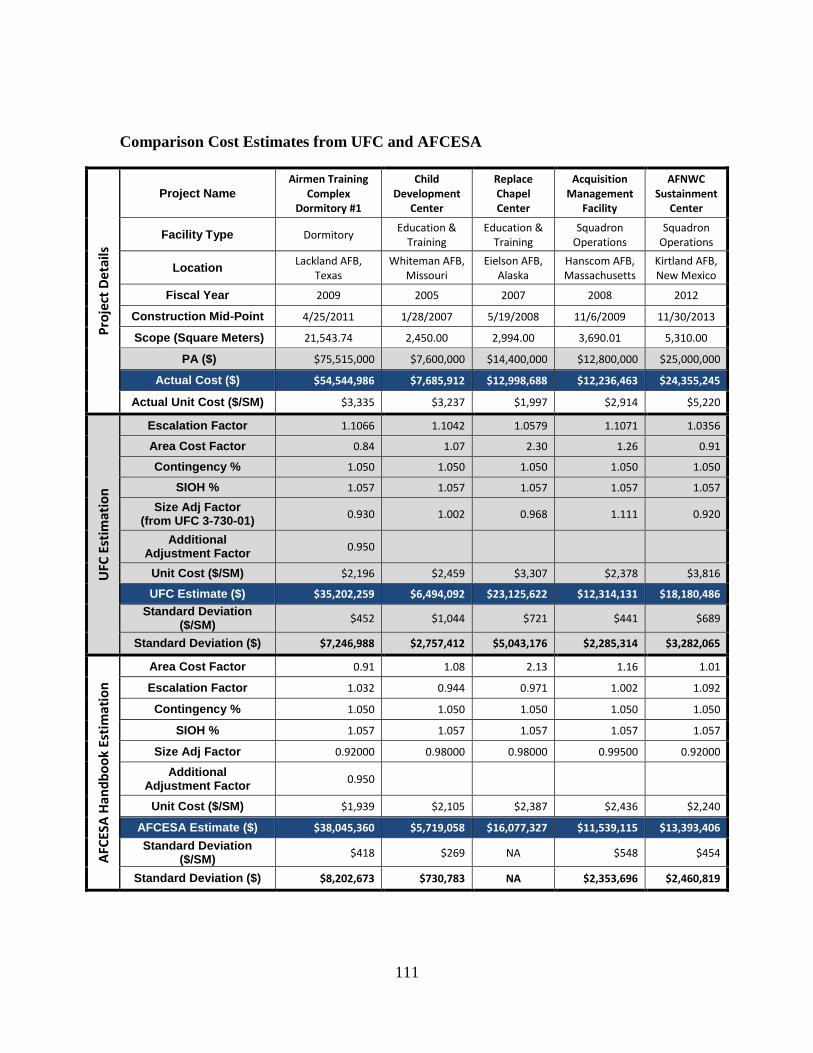
111
Comparison Cost Estimates from UFC and AFCESA
Pro
ject
De
tails
Project Name
Airmen Training Complex
Dormitory #1
Child Development
Center
Replace Chapel Center
Acquisition Management
Facility
AFNWC Sustainment
Center
Facility Type Dormitory Education &
Training Education &
Training Squadron
Operations Squadron
Operations
Location Lackland AFB,
Texas Whiteman AFB,
Missouri Eielson AFB,
Alaska Hanscom AFB, Massachusetts
Kirtland AFB, New Mexico
Fiscal Year 2009 2005 2007 2008 2012
Construction Mid-Point 4/25/2011 1/28/2007 5/19/2008 11/6/2009 11/30/2013
Scope (Square Meters) 21,543.74 2,450.00 2,994.00 3,690.01 5,310.00
PA ($) $75,515,000 $7,600,000 $14,400,000 $12,800,000 $25,000,000
Actual Cost ($) $54,544,986 $7,685,912 $12,998,688 $12,236,463 $24,355,245
Actual Unit Cost ($/SM) $3,335 $3,237 $1,997 $2,914 $5,220
UFC
Est
imat
ion
Escalation Factor 1.1066 1.1042 1.0579 1.1071 1.0356
Area Cost Factor 0.84 1.07 2.30 1.26 0.91
Contingency % 1.050 1.050 1.050 1.050 1.050
SIOH % 1.057 1.057 1.057 1.057 1.057
Size Adj Factor (from UFC 3-730-01)
0.930 1.002 0.968 1.111 0.920
Additional Adjustment Factor
0.950
Unit Cost ($/SM) $2,196 $2,459 $3,307 $2,378 $3,816
UFC Estimate ($) $35,202,259 $6,494,092 $23,125,622 $12,314,131 $18,180,486
Standard Deviation ($/SM)
$452 $1,044 $721 $441 $689
Standard Deviation ($) $7,246,988 $2,757,412 $5,043,176 $2,285,314 $3,282,065
AFC
ESA
Han
db
oo
k Es
tim
atio
n
Area Cost Factor 0.91 1.08 2.13 1.16 1.01
Escalation Factor 1.032 0.944 0.971 1.002 1.092
Contingency % 1.050 1.050 1.050 1.050 1.050
SIOH % 1.057 1.057 1.057 1.057 1.057
Size Adj Factor 0.92000 0.98000 0.98000 0.99500 0.92000
Additional Adjustment Factor
0.950
Unit Cost ($/SM) $1,939 $2,105 $2,387 $2,436 $2,240
AFCESA Estimate ($) $38,045,360 $5,719,058 $16,077,327 $11,539,115 $13,393,406
Standard Deviation ($/SM)
$418 $269 NA $548 $454
Standard Deviation ($) $8,202,673 $730,783 NA $2,353,696 $2,460,819
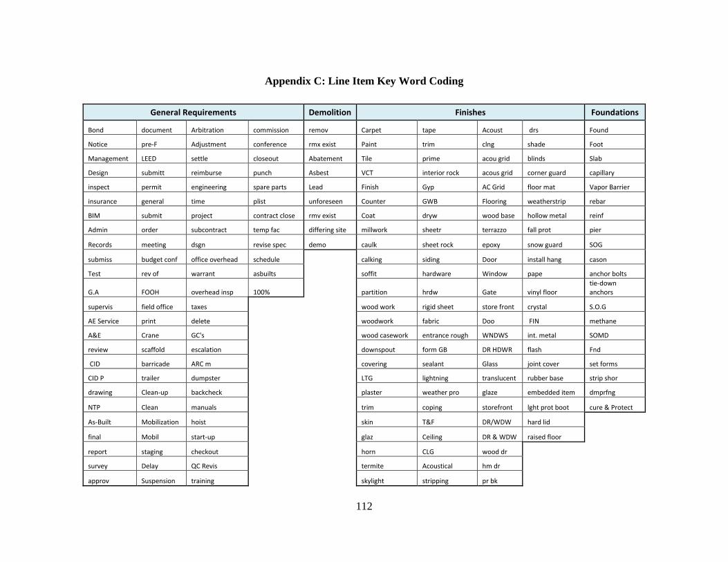
112
Appendix C: Line Item Key Word Coding
General Requirements Demolition Finishes Foundations
Bond document Arbitration commission remov Carpet tape Acoust drs Found
Notice pre-F Adjustment conference rmx exist Paint trim clng shade Foot
Management LEED settle closeout Abatement Tile prime acou grid blinds Slab
Design submitt reimburse punch Asbest VCT interior rock acous grid corner guard capillary
inspect permit engineering spare parts Lead Finish Gyp AC Grid floor mat Vapor Barrier
insurance general time plist unforeseen Counter GWB Flooring weatherstrip rebar
BIM submit project contract close rmv exist Coat dryw wood base hollow metal reinf
Admin order subcontract temp fac differing site millwork sheetr terrazzo fall prot pier
Records meeting dsgn revise spec demo caulk sheet rock epoxy snow guard SOG
submiss budget conf office overhead schedule
calking siding Door install hang cason
Test rev of warrant asbuilts
soffit hardware Window pape anchor bolts
G.A FOOH overhead insp 100%
partition hrdw Gate vinyl floor tie-down anchors
supervis field office taxes
wood work rigid sheet store front crystal S.O.G
AE Service print delete
woodwork fabric Doo FIN methane
A&E Crane GC's
wood casework entrance rough WNDWS int. metal SOMD
review scaffold escalation
downspout form GB DR HDWR flash Fnd
CID barricade ARC m
covering sealant Glass joint cover set forms
CID P trailer dumpster
LTG lightning translucent rubber base strip shor
drawing Clean-up backcheck
plaster weather pro glaze embedded item dmprfng
NTP Clean manuals
trim coping storefront lght prot boot cure & Protect
As-Built Mobilization hoist
skin T&F DR/WDW hard lid
final Mobil start-up
glaz Ceiling DR & WDW raised floor
report staging checkout
horn CLG wood dr
survey Delay QC Revis
termite Acoustical hm dr
approv Suspension training
skylight stripping pr bk
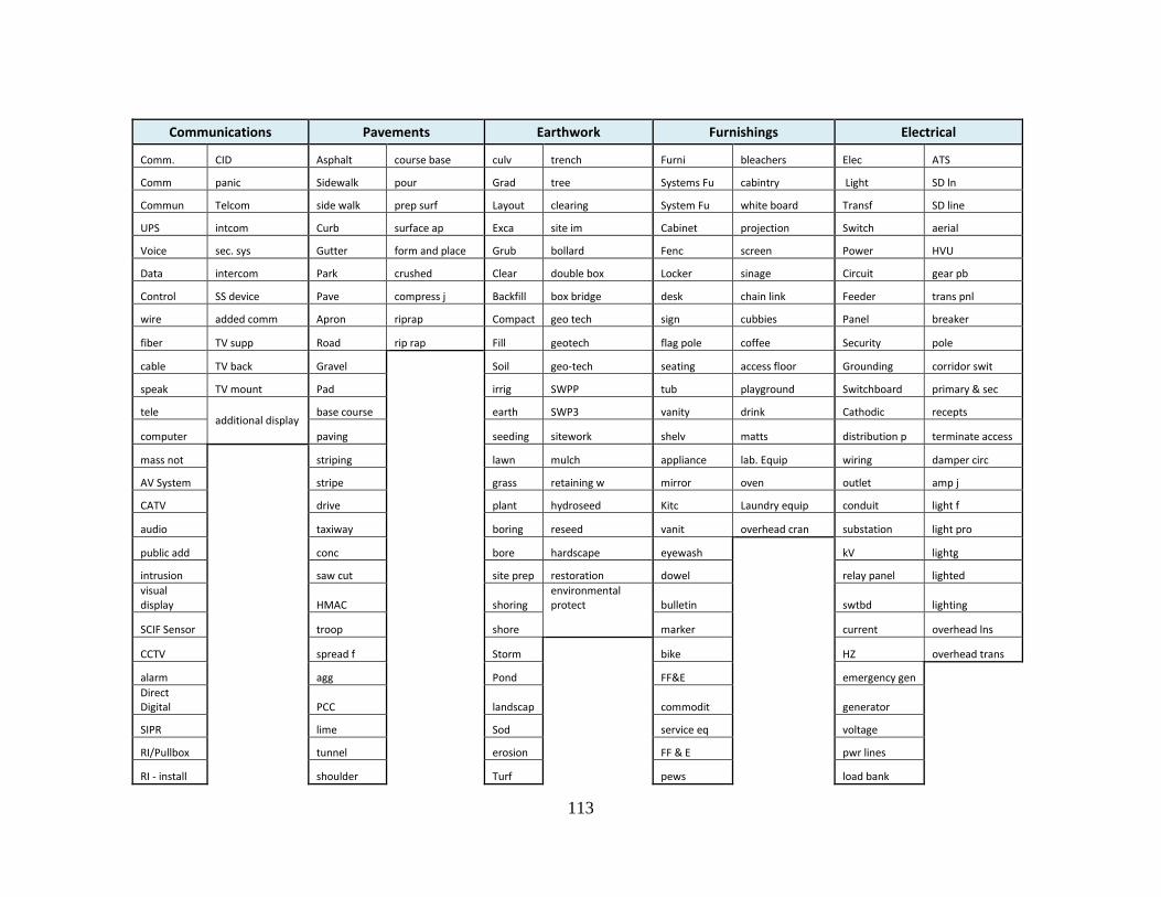
113
Communications Pavements Earthwork Furnishings Electrical
Comm. CID Asphalt course base culv trench Furni bleachers Elec ATS
Comm panic Sidewalk pour Grad tree Systems Fu cabintry Light SD ln
Commun Telcom side walk prep surf Layout clearing System Fu white board Transf SD line
UPS intcom Curb surface ap Exca site im Cabinet projection Switch aerial
Voice sec. sys Gutter form and place Grub bollard Fenc screen Power HVU
Data intercom Park crushed Clear double box Locker sinage Circuit gear pb
Control SS device Pave compress j Backfill box bridge desk chain link Feeder trans pnl
wire added comm Apron riprap Compact geo tech sign cubbies Panel breaker
fiber TV supp Road rip rap Fill geotech flag pole coffee Security pole
cable TV back Gravel
Soil geo-tech seating access floor Grounding corridor swit
speak TV mount Pad
irrig SWPP tub playground Switchboard primary & sec
tele additional display
base course
earth SWP3 vanity drink Cathodic recepts
computer paving
seeding sitework shelv matts distribution p terminate access
mass not
striping
lawn mulch appliance lab. Equip wiring damper circ
AV System
stripe
grass retaining w mirror oven outlet amp j
CATV
drive
plant hydroseed Kitc Laundry equip conduit light f
audio
taxiway
boring reseed vanit overhead cran substation light pro
public add
conc
bore hardscape eyewash
kV lightg
intrusion
saw cut
site prep restoration dowel
relay panel lighted
visual display
HMAC
shoring
environmental protect bulletin
swtbd lighting
SCIF Sensor
troop
shore marker
current overhead lns
CCTV
spread f
Storm
bike
HZ overhead trans
alarm
agg
Pond
FF&E
emergency gen Direct
Digital
PCC
landscap
commodit
generator
SIPR
lime
Sod
service eq
voltage
RI/Pullbox
tunnel
erosion
FF & E
pwr lines
RI - install
shoulder
Turf
pews
load bank
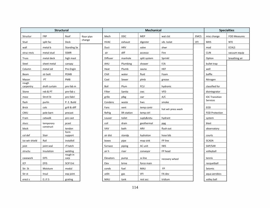
114
Structural Mechanical Specialties
Structur FRP Roof floor plan change
Mech DDC MEP wat clst EMCS misc change FOD Measures
Stud split fac Deck HVAC exhaust digester vib. Isolat VFI MHS NTE
wall metal b Standing Se
Duct HRV valve shwr
mod ECALS
struc revis metal stud SSMR
air diff accesso Fire
CLIN vacuum equip
Truss metal deck high mast
Diffuser manhole split system Sprinkl
Option breathing air
Steel sheet metal canopy
AHU Plumbing shower F/A
bullet trap
Column metal sid Pre-Engin
Heat Plumb sauna HEF
well
Beam str bolt PEMB
Chill water fluid Foam
baffle
Mason PT PMB
Cool Sewer plmb grease
Nitrogen rough
carpentry draft curtain pre-fab m
Boil Plum FCU hydronic
classified for
Stone reb & PT pre-fab s
Filter Sanita cws VFD
disintegrator
mezz Strctl St pre-fabri
grille plbg cwr A/C
IOC Transition Services
flash purlin P. E. Build
Condens waste hws smoke
Brick cols grill & diff
Fans vent temp contr hot wtr press wash
EOD
CMU pole barn precast
Refrig lift station temp ctrl
FOD Protection
Fram catwalk pre cast
Louver toilet suply&retu hydrant
system
stucc temporary
construct
pcast
coil drain geothermal ppg
blast
block tendon
VAV bath ARV flush out
observatory
col def Stair form support
air dist standp hydration hose bib
courts
ice wtr shield Rail installstl
boxes pipe mop sink FP line
SCADA
joist joint seal rf hatch
furnace piping AC unit IWS
SAP/SAR
structu Insulation welding
air h riser conveyor FP head
volleyball
casework EIFS rough in carp
Elevators pump ss line recovery wheel
tennis
ICF EFIS SCIF Ent
Elev brine force main
racquetball
Str. St Moisture modul
conds fuel MAU FP
Seismic
Str st Insul exp joint
utilit gas VFI FA dev
aqua aerobics
erect s E.I.F.S grating
MAU tank rest acc tridium
volley ball
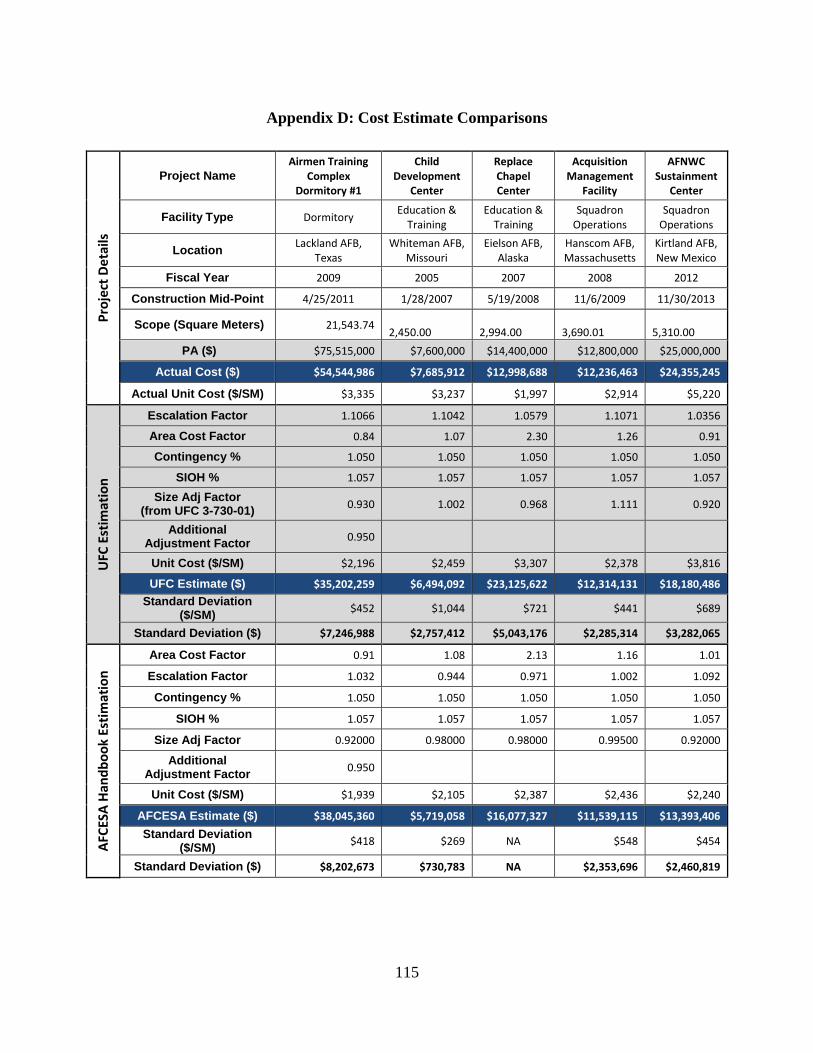
115
Appendix D: Cost Estimate Comparisons P
roje
ct D
eta
ils
Project Name
Airmen Training Complex
Dormitory #1
Child Development
Center
Replace Chapel Center
Acquisition Management
Facility
AFNWC Sustainment
Center
Facility Type Dormitory Education &
Training Education &
Training Squadron
Operations Squadron
Operations
Location Lackland AFB,
Texas Whiteman AFB,
Missouri Eielson AFB,
Alaska Hanscom AFB, Massachusetts
Kirtland AFB, New Mexico
Fiscal Year 2009 2005 2007 2008 2012
Construction Mid-Point 4/25/2011 1/28/2007 5/19/2008 11/6/2009 11/30/2013
Scope (Square Meters) 21,543.74 2,450.00
2,994.00
3,690.01
5,310.00
PA ($) $75,515,000 $7,600,000 $14,400,000 $12,800,000 $25,000,000
Actual Cost ($) $54,544,986 $7,685,912 $12,998,688 $12,236,463 $24,355,245
Actual Unit Cost ($/SM) $3,335 $3,237 $1,997 $2,914 $5,220
UFC
Est
imat
ion
Escalation Factor 1.1066 1.1042 1.0579 1.1071 1.0356
Area Cost Factor 0.84 1.07 2.30 1.26 0.91
Contingency % 1.050 1.050 1.050 1.050 1.050
SIOH % 1.057 1.057 1.057 1.057 1.057
Size Adj Factor (from UFC 3-730-01)
0.930 1.002 0.968 1.111 0.920
Additional Adjustment Factor
0.950
Unit Cost ($/SM) $2,196 $2,459 $3,307 $2,378 $3,816
UFC Estimate ($) $35,202,259 $6,494,092 $23,125,622 $12,314,131 $18,180,486
Standard Deviation ($/SM)
$452 $1,044 $721 $441 $689
Standard Deviation ($) $7,246,988 $2,757,412 $5,043,176 $2,285,314 $3,282,065
AFC
ESA
Han
db
oo
k Es
tim
atio
n
Area Cost Factor 0.91 1.08 2.13 1.16 1.01
Escalation Factor 1.032 0.944 0.971 1.002 1.092
Contingency % 1.050 1.050 1.050 1.050 1.050
SIOH % 1.057 1.057 1.057 1.057 1.057
Size Adj Factor 0.92000 0.98000 0.98000 0.99500 0.92000
Additional Adjustment Factor
0.950
Unit Cost ($/SM) $1,939 $2,105 $2,387 $2,436 $2,240
AFCESA Estimate ($) $38,045,360 $5,719,058 $16,077,327 $11,539,115 $13,393,406
Standard Deviation ($/SM)
$418 $269 NA $548 $454
Standard Deviation ($) $8,202,673 $730,783 NA $2,353,696 $2,460,819
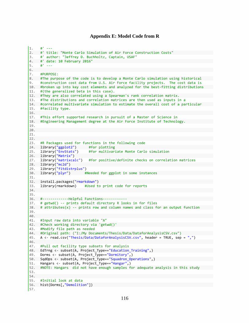
116
Appendix E: Model Code from R
1. #' --- 2. #' title: "Monte Carlo Simulation of Air Force Construction Costs" 3. #' author: "Jeffrey D. Buchholtz, Captain, USAF" 4. #' date: 10 February 2016" 5. #' --- 6. 7. #PURPOSE: 8. #The purpose of the code is to develop a Monte Carlo simulation using historical 9. #construction cost data from U.S. Air Force facility projects. The cost data is 10. #broken up into key cost elements and analyzed for the best-fitting distributions 11. #(the generalized beta in this case). 12. #They are also correlated using a Spearman's rank correlation matrix. 13. #The distributions and correlation matrices are then used as inputs in a 14. #correlated multivariate simulation to estimate the overall cost of a particular 15. #facility type. 16. 17. #This effort supported research in pursuit of a Master of Science in 18. #Engineering Management degree at the Air Force Institute of Technology. 19. 20. 21. 22. 23. #R Packages used for functions in the following code 24. library("ggplot2") #for plotting 25. library("EnvStats") #for multivariate Monte Carlo simulation 26. library("Matrix") 27. library("matrixcalc") #for positive/definite checks on correlation matrices 28. library("mc2d") 29. library("fitdistrplus") 30. library("plyr") #Needed for ggplot in some instances 31. 32. install.packages("rmarkdown") 33. library(rmarkdown) #Used to print code for reports 34. 35. 36. #-------------Helpful Functions------------ 37. # getwd() -- prints default directory R looks in for files 38. # attributes(x) -- prints row and column names and class for an output function 39. 40. 41. #Input raw data into variable "A" 42. #Check working directory via 'getwd()' 43. #Modify file path as needed 44. #Original path: ("I:/My Documents/Thesis/Data/DataforAnalysisCSV.csv") 45. A <- read.csv("Thesis/Data/DataforAnalysisCSV.csv", header = TRUE, sep = ",") 46. 47. #Pull out facility type subsets for analysis 48. EdTrng <- subset(A, Project_Type=="Education_Training",) 49. Dorms <- subset(A, Project_Type=="Dormitory",) 50. SqdOps <- subset(A, Project_Type=="Squadron_Operations",) 51. Hangars <- subset(A, Project_Type=="Hangar",) 52. #NOTE: Hangars did not have enough samples for adequate analysis in this study 53. 54. 55. #Initial look at data 56. hist(Dorms[,"Demolition"]) 57.

117
58. #more complete look using histograms and density functions 59. m <-
ggplot(EdTrng, aes(x=Earthwork)) #saves data to be plotted in "m" 60. m + geom_histogram(bandwidth=50) #plots histogram with set width 61. m + geom_histogram(aes(y = ..density..),binwidth=50) + geom_density() 62. #plots histogram versus probability density (instead of count) along with curve 63. 64. 65. # compare cost CUONT between facility types 66. m <- ggplot(A, aes(x=Structural)) #get Structural data for plot 67. m <- m + geom_histogram(binwidth = 50) #get histogram w/ width 68. m + facet_wrap( ~ Project_Type, ncol=2) #plot by project type in 2 col 69. 70. #compare cost DENSITY between facility types 71. m <- ggplot(A, aes(x=Structural)) #get Structural data for plot 72. m <- m + geom_histogram(binwidth = 50) + aes(y = ..density..) + geom_density() 73. #get histogram w/ width by density with density curve 74. m + facet_wrap( ~ Project_Type, ncol=2) #plot by project type in 2 col 75. 76. #adding color and labels along with density together in one saved plot 77. plot_Structural = ggplot(A, aes(x=Structural, fill=Project_Type)) + 78. geom_histogram(colour="grey30", binwidth=50) + 79. aes(y = ..density..) + 80. geom_density(alpha=.2) + 81. facet_grid(Project_Type ~ .) + 82. labs(title="Histograms") 83. plot_Structural 84. 85. #Distribution Fitting 86. SqdOps.Struc15 <- SqdOps[,15] #pulls out Structural costs from Squad Ops 87. descdist(SqdOps.Struc15) # Plots observed data versus common distributions 88. descdist(SqdOps.Struc15, boot = 1000) # same as above but also plots 89. #potential variation in observed data 90. 91. 92. #Pull out each cost column as a separate variable for analysis 93. EdTrng.GenReq <- EdTrng[,14] 94. EdTrng.Demo <- EdTrng[,15] 95. EdTrng.Finish <- EdTrng[,16] 96. EdTrng.Found <- EdTrng[,17] 97. EdTrng.Comm <- EdTrng[,18] 98. EdTrng.Earth <- EdTrng[,19] 99. EdTrng.Furnish <- EdTrng[,20] 100. EdTrng.Elec <- EdTrng[,21] 101. EdTrng.Struct <- EdTrng[,22] 102. EdTrng.Mech <- EdTrng[,23] 103. EdTrng.Spec <- EdTrng[,24] 104. 105. Dorms.GenReq <- Dorms[,14] 106. Dorms.Demo <- Dorms[,15] 107. Dorms.Finish <- Dorms[,16] 108. Dorms.Found <- Dorms[,17] 109. Dorms.Comm <- Dorms[,18] 110. Dorms.Earth <- Dorms[,19] 111. Dorms.Furnish <- Dorms[,20] 112. Dorms.Elec <- Dorms[,21] 113. Dorms.Struct <- Dorms[,22] 114. Dorms.Mech <- Dorms[,23] 115. Dorms.Spec <- Dorms[,24] 116.

118
117. SqdOps.GenReq <- SqdOps[,14] 118. SqdOps.Demo <- SqdOps[,15] 119. SqdOps.Finish <- SqdOps[,16] 120. SqdOps.Found <- SqdOps[,17] 121. SqdOps.Comm <- SqdOps[,18] 122. SqdOps.Earth <- SqdOps[,19] 123. SqdOps.Furnish <- SqdOps[,20] 124. SqdOps.Elec <- SqdOps[,21] 125. SqdOps.Struct <- SqdOps[,22] 126. SqdOps.Mech <- SqdOps[,23] 127. SqdOps.Spec <- SqdOps[,24] 128. 129. 130. #Pull out overall costs as a matrix variable for analysis 131. EdTrng.Costs <- EdTrng[,14:24] 132. Dorms.Costs <- Dorms[,14:24] 133. SqdOps.Costs <- SqdOps[,14:24] 134. 135. #Graph each cost column to identify probable distribution matches. 136. ##Include "boot = x" to display x runs of sample from the data 137. ##with replacement to see the bootstrap variation range on the graph 138. descdist(EdTrng.GenReq, boot = 1000) 139. descdist(EdTrng.Demo, boot = 1000) 140. descdist(EdTrng.Finish, boot = 1000) 141. descdist(EdTrng.Found, boot = 1000) 142. descdist(EdTrng.Comm, boot = 1000) 143. descdist(EdTrng.Earth, boot = 1000) 144. descdist(EdTrng.Furnish, boot = 1000) 145. descdist(EdTrng.Elec, boot = 1000) 146. descdist(EdTrng.Struct, boot = 1000) 147. descdist(EdTrng.Mech, boot = 1000) 148. descdist(EdTrng.Spec, boot = 1000) 149. 150. descdist(Dorms.GenReq, boot = 1000) 151. descdist(Dorms.Demo, boot = 1000) 152. descdist(Dorms.Finish, boot = 1000) 153. descdist(Dorms.Found, boot = 1000) 154. descdist(Dorms.Comm, boot = 1000) 155. descdist(Dorms.Earth, boot = 1000) 156. descdist(Dorms.Furnish, boot = 1000) 157. descdist(Dorms.Elec, boot = 1000) 158. descdist(Dorms.Struct, boot = 1000) 159. descdist(Dorms.Mech, boot = 1000) 160. descdist(Dorms.Spec, boot = 1000) 161. 162. descdist(SqdOps.GenReq, boot = 1000) 163. descdist(SqdOps.Demo, boot = 1000) 164. descdist(SqdOps.Finish, boot = 1000) 165. descdist(SqdOps.Found, boot = 1000) 166. descdist(SqdOps.Comm, boot = 1000) 167. descdist(SqdOps.Earth, boot = 1000) 168. descdist(SqdOps.Furnish, boot = 1000) 169. descdist(SqdOps.Elec, boot = 1000) 170. descdist(SqdOps.Struct, boot = 1000) 171. descdist(SqdOps.Mech, boot = 1000) 172. descdist(SqdOps.Spec, boot = 1000) 173. 174. 175. 176. #K-S Goodness of Fit test (requires "stats" package) to get p-value

119
177. 178. ##Input parameters for analysis 179. Distro.Params <- read.csv("Thesis/Data/DistroParams.csv", header = TRUE, sep = ",") 180. 181. ##Save parameters based on facility type 182. EdTrng.Params <- data.matrix(Distro.Params[12:22,], rownames.force = NA) 183. Dorms.Params <- data.matrix(Distro.Params[1:11,], rownames.force = NA) 184. SqdOps.Params <- data.matrix(Distro.Params[23:33,], rownames.force = NA) 185. 186. ##Transform data to standardized beta by shifting and scaling 187. ##NOTE: if there are repeat values (such as 0), 188. #they must be changed slightly for the KS test (no ties allowed) 189. EdTrng.GenReq.Beta <- (EdTrng.GenReq - 190. EdTrng.Params[1,"Loc_Shift"]) / EdTrng.Params[1,"Scaler"] 191. EdTrng.Demo.Beta <- (EdTrng.Demo - 192. EdTrng.Params[2,"Loc_Shift"]) / EdTrng.Params[2,"Scaler"] 193. EdTrng.Finish.Beta <- (EdTrng.Finish - 194. EdTrng.Params[3,"Loc_Shift"]) / EdTrng.Params[3,"Scaler"] 195. EdTrng.Found.Beta <- (EdTrng.Found - 196. EdTrng.Params[4,"Loc_Shift"]) / EdTrng.Params[4,"Scaler"] 197. EdTrng.Comm.Beta <- (EdTrng.Comm - 198. EdTrng.Params[5,"Loc_Shift"]) / EdTrng.Params[5,"Scaler"] 199. EdTrng.Earth.Beta <- (EdTrng.Earth - 200. EdTrng.Params[6,"Loc_Shift"]) / EdTrng.Params[6,"Scaler"] 201. EdTrng.Furnish.Beta <- (EdTrng.Furnish - 202. EdTrng.Params[7,"Loc_Shift"]) / EdTrng.Params[7,"Scaler"] 203. EdTrng.Elec.Beta <- (EdTrng.Elec - 204. EdTrng.Params[8,"Loc_Shift"]) / EdTrng.Params[8,"Scaler"] 205. EdTrng.Struct.Beta <- (EdTrng.Struct - 206. EdTrng.Params[9,"Loc_Shift"]) / EdTrng.Params[9,"Scaler"] 207. EdTrng.Mech.Beta <- (EdTrng.Mech - 208. EdTrng.Params[10,"Loc_Shift"]) / EdTrng.Params[10,"Scaler"] 209. EdTrng.Spec.Beta <- (EdTrng.Spec - 210. EdTrng.Params[11,"Loc_Shift"]) / EdTrng.Params[11,"Scaler"] 211. EdTrng.Spec.Beta[12] <- EdTrng.Spec.Beta[12] + 0.00000001 212. 213. Dorms.GenReq.Beta <- (Dorms.GenReq - 214. Dorms.Params[1,"Loc_Shift"]) / Dorms.Params[1,"Scaler"] 215. Dorms.Demo.Beta <- (Dorms.Demo - 216. Dorms.Params[2,"Loc_Shift"]) / Dorms.Params[2,"Scaler"] 217. Dorms.Demo.Beta[2] <- Dorms.Demo.Beta[2] + 0.00000001 218. Dorms.Demo.Beta[4] <- Dorms.Demo.Beta[4] + 0.00000002 219. Dorms.Finish.Beta <- (Dorms.Finish - 220. Dorms.Params[3,"Loc_Shift"]) / Dorms.Params[3,"Scaler"] 221. Dorms.Found.Beta <- (Dorms.Found - 222. Dorms.Params[4,"Loc_Shift"]) / Dorms.Params[4,"Scaler"] 223. Dorms.Comm.Beta <- (Dorms.Comm - 224. Dorms.Params[5,"Loc_Shift"]) / Dorms.Params[5,"Scaler"] 225. Dorms.Earth.Beta <- (Dorms.Earth - 226. Dorms.Params[6,"Loc_Shift"]) / Dorms.Params[6,"Scaler"] 227. Dorms.Furnish.Beta <- (Dorms.Furnish - 228. Dorms.Params[7,"Loc_Shift"]) / Dorms.Params[7,"Scaler"] 229. Dorms.Elec.Beta <- (Dorms.Elec - 230. Dorms.Params[8,"Loc_Shift"]) / Dorms.Params[8,"Scaler"] 231. Dorms.Struct.Beta <- (Dorms.Struct - 232. Dorms.Params[9,"Loc_Shift"]) / Dorms.Params[9,"Scaler"] 233. Dorms.Mech.Beta <- (Dorms.Mech - 234. Dorms.Params[10,"Loc_Shift"]) / Dorms.Params[10,"Scaler"] 235. Dorms.Spec.Beta <- (Dorms.Spec - 236. Dorms.Params[11,"Loc_Shift"]) / Dorms.Params[11,"Scaler"]
120
237. 238. SqdOps.GenReq.Beta <- (SqdOps.GenReq - 239. SqdOps.Params[1,"Loc_Shift"]) / SqdOps.Params[1,"Scaler"] 240. SqdOps.Demo.Beta <- (SqdOps.Demo - 241. SqdOps.Params[2,"Loc_Shift"]) / SqdOps.Params[2,"Scaler"] 242. SqdOps.Finish.Beta <- (SqdOps.Finish - 243. SqdOps.Params[3,"Loc_Shift"]) / SqdOps.Params[3,"Scaler"] 244. SqdOps.Found.Beta <- (SqdOps.Found - 245. SqdOps.Params[4,"Loc_Shift"]) / SqdOps.Params[4,"Scaler"] 246. SqdOps.Comm.Beta <- (SqdOps.Comm - 247. SqdOps.Params[5,"Loc_Shift"]) / SqdOps.Params[5,"Scaler"] 248. SqdOps.Earth.Beta <- (SqdOps.Earth - 249. SqdOps.Params[6,"Loc_Shift"]) / SqdOps.Params[6,"Scaler"] 250. SqdOps.Furnish.Beta <- (SqdOps.Furnish - 251. SqdOps.Params[7,"Loc_Shift"]) / SqdOps.Params[7,"Scaler"] 252. SqdOps.Elec.Beta <- (SqdOps.Elec - 253. SqdOps.Params[8,"Loc_Shift"]) / SqdOps.Params[8,"Scaler"] 254. SqdOps.Struct.Beta <- (SqdOps.Struct - 255. SqdOps.Params[9,"Loc_Shift"]) / SqdOps.Params[9,"Scaler"] 256. SqdOps.Mech.Beta <- (SqdOps.Mech - 257. SqdOps.Params[10,"Loc_Shift"]) / SqdOps.Params[10,"Scaler"] 258. SqdOps.Spec.Beta <- (SqdOps.Spec - 259. SqdOps.Params[11,"Loc_Shift"]) / SqdOps.Params[11,"Scaler"] 260. 261. 262. ##Perform Kolmogorov-Smirnov Goodness of Fit Test 263. #for each distribution and save restults 264. EdTrng.GenReq.KS <- ks.test(EdTrng.GenReq.Beta, "pbeta", 265. EdTrng.Params[1,"Alpha"], 266. EdTrng.Params[1,"Beta"]) 267. EdTrng.Demo.KS <- ks.test(EdTrng.Demo.Beta, "pbeta", 268. EdTrng.Params[2,"Alpha"], 269. EdTrng.Params[2,"Beta"]) 270. EdTrng.Finish.KS <- ks.test(EdTrng.Finish.Beta, "pbeta", 271. EdTrng.Params[3,"Alpha"], 272. EdTrng.Params[3,"Beta"]) 273. EdTrng.Found.KS <- ks.test(EdTrng.Found.Beta, "pbeta", 274. EdTrng.Params[4,"Alpha"], 275. EdTrng.Params[4,"Beta"]) 276. EdTrng.Comm.KS <- ks.test(EdTrng.Comm.Beta, "pbeta", 277. EdTrng.Params[5,"Alpha"], 278. EdTrng.Params[5,"Beta"]) 279. EdTrng.Earth.KS <- ks.test(EdTrng.Earth.Beta, "pbeta", 280. EdTrng.Params[6,"Alpha"], 281. EdTrng.Params[6,"Beta"]) 282. EdTrng.Furnish.KS <- ks.test(EdTrng.Furnish.Beta, "pbeta", 283. EdTrng.Params[7,"Alpha"], 284. EdTrng.Params[7,"Beta"]) 285. EdTrng.Elec.KS <- ks.test(EdTrng.Elec.Beta, "pbeta", 286. EdTrng.Params[8,"Alpha"], 287. EdTrng.Params[8,"Beta"]) 288. EdTrng.Struct.KS <- ks.test(EdTrng.Struct.Beta, "pbeta", 289. EdTrng.Params[9,"Alpha"], 290. EdTrng.Params[9,"Beta"]) 291. EdTrng.Mech.KS <- ks.test(EdTrng.Mech.Beta, "pbeta", 292. EdTrng.Params[10,"Alpha"], 293. EdTrng.Params[10,"Beta"]) 294. EdTrng.Spec.KS <- ks.test(EdTrng.Spec.Beta, "pbeta", 295. EdTrng.Params[11,"Alpha"], 296. EdTrng.Params[11,"Beta"])
121
297. 298. Dorms.GenReq.KS <- ks.test(Dorms.GenReq.Beta, "pbeta", 299. Dorms.Params[1,"Alpha"], 300. Dorms.Params[1,"Beta"]) 301. Dorms.Demo.KS <- ks.test(Dorms.Demo.Beta, "pbeta", 302. Dorms.Params[2,"Alpha"], 303. Dorms.Params[2,"Beta"]) 304. Dorms.Finish.KS <- ks.test(Dorms.Finish.Beta, "pbeta", 305. Dorms.Params[3,"Alpha"], 306. Dorms.Params[3,"Beta"]) 307. Dorms.Found.KS <- ks.test(Dorms.Found.Beta, "pbeta", 308. Dorms.Params[4,"Alpha"], 309. Dorms.Params[4,"Beta"]) 310. Dorms.Comm.KS <- ks.test(Dorms.Comm.Beta, "pbeta", 311. Dorms.Params[5,"Alpha"], 312. Dorms.Params[5,"Beta"]) 313. Dorms.Earth.KS <- ks.test(Dorms.Earth.Beta, "pbeta", 314. Dorms.Params[6,"Alpha"], 315. Dorms.Params[6,"Beta"]) 316. Dorms.Furnish.KS <- ks.test(Dorms.Furnish.Beta, "pbeta", 317. Dorms.Params[7,"Alpha"], 318. Dorms.Params[7,"Beta"]) 319. Dorms.Elec.KS <- ks.test(Dorms.Elec.Beta, "pbeta", 320. Dorms.Params[8,"Alpha"], 321. Dorms.Params[8,"Beta"]) 322. Dorms.Struct.KS <- ks.test(Dorms.Struct.Beta, "pbeta", 323. Dorms.Params[9,"Alpha"], 324. Dorms.Params[9,"Beta"]) 325. Dorms.Mech.KS <- ks.test(Dorms.Mech.Beta, "pbeta", 326. Dorms.Params[10,"Alpha"], 327. Dorms.Params[10,"Beta"]) 328. Dorms.Spec.KS <- ks.test(Dorms.Spec.Beta, "pbeta", 329. Dorms.Params[11,"Alpha"], 330. Dorms.Params[11,"Beta"]) 331. 332. SqdOps.GenReq.KS <- ks.test(SqdOps.GenReq.Beta, "pbeta", 333. SqdOps.Params[1,"Alpha"], 334. SqdOps.Params[1,"Beta"]) 335. SqdOps.Demo.KS <- ks.test(SqdOps.Demo.Beta, "pbeta", 336. SqdOps.Params[2,"Alpha"], 337. SqdOps.Params[2,"Beta"]) 338. SqdOps.Finish.KS <- ks.test(SqdOps.Finish.Beta, "pbeta", 339. SqdOps.Params[3,"Alpha"], 340. SqdOps.Params[3,"Beta"]) 341. SqdOps.Found.KS <- ks.test(SqdOps.Found.Beta, "pbeta", 342. SqdOps.Params[4,"Alpha"], 343. SqdOps.Params[4,"Beta"]) 344. SqdOps.Comm.KS <- ks.test(SqdOps.Comm.Beta, "pbeta", 345. SqdOps.Params[5,"Alpha"], 346. SqdOps.Params[5,"Beta"]) 347. SqdOps.Earth.KS <- ks.test(SqdOps.Earth.Beta, "pbeta", 348. SqdOps.Params[6,"Alpha"], 349. SqdOps.Params[6,"Beta"]) 350. SqdOps.Furnish.KS <- ks.test(SqdOps.Furnish.Beta, "pbeta", 351. SqdOps.Params[7,"Alpha"], 352. SqdOps.Params[7,"Beta"]) 353. SqdOps.Elec.KS <- ks.test(SqdOps.Elec.Beta, "pbeta", 354. SqdOps.Params[8,"Alpha"], 355. SqdOps.Params[8,"Beta"]) 356. SqdOps.Struct.KS <- ks.test(SqdOps.Struct.Beta, "pbeta",
122
357. SqdOps.Params[9,"Alpha"], 358. SqdOps.Params[9,"Beta"]) 359. SqdOps.Mech.KS <- ks.test(SqdOps.Mech.Beta, "pbeta", 360. SqdOps.Params[10,"Alpha"], 361. SqdOps.Params[10,"Beta"]) 362. SqdOps.Spec.KS <- ks.test(SqdOps.Spec.Beta, "pbeta", 363. SqdOps.Params[11,"Alpha"], 364. SqdOps.Params[11,"Beta"]) 365. 366. 367. #Save KS test restults into lists and combine into a dataframe 368. KS.CostElement <- as.vector(1:33) 369. KS.Statistic <- as.vector(1:33) 370. KS.Pvalue <- as.vector(1:33) 371. 372. ##Save Cost Element Names 373. KS.CostElement[1] <- c(EdTrng.GenReq.KS$data.name) 374. KS.CostElement[2] <- c(EdTrng.Demo.KS$data.name) 375. KS.CostElement[3] <- c(EdTrng.Finish.KS$data.name) 376. KS.CostElement[4] <- c(EdTrng.Found.KS$data.name) 377. KS.CostElement[5] <- c(EdTrng.Comm.KS$data.name) 378. KS.CostElement[6] <- c(EdTrng.Earth.KS$data.name) 379. KS.CostElement[7] <- c(EdTrng.Furnish.KS$data.name) 380. KS.CostElement[8] <- c(EdTrng.Elec.KS$data.name) 381. KS.CostElement[9] <- c(EdTrng.Struct.KS$data.name) 382. KS.CostElement[10] <- c(EdTrng.Mech.KS$data.name) 383. KS.CostElement[11] <- c(EdTrng.Spec.KS$data.name) 384. 385. KS.CostElement[12] <- c(Dorms.GenReq.KS$data.name) 386. KS.CostElement[13] <- c(Dorms.Demo.KS$data.name) 387. KS.CostElement[14] <- c(Dorms.Finish.KS$data.name) 388. KS.CostElement[15] <- c(Dorms.Found.KS$data.name) 389. KS.CostElement[16] <- c(Dorms.Comm.KS$data.name) 390. KS.CostElement[17] <- c(Dorms.Earth.KS$data.name) 391. KS.CostElement[18] <- c(Dorms.Furnish.KS$data.name) 392. KS.CostElement[19] <- c(Dorms.Elec.KS$data.name) 393. KS.CostElement[20] <- c(Dorms.Struct.KS$data.name) 394. KS.CostElement[21] <- c(Dorms.Mech.KS$data.name) 395. KS.CostElement[22] <- c(Dorms.Spec.KS$data.name) 396. 397. KS.CostElement[23] <- c(SqdOps.GenReq.KS$data.name) 398. KS.CostElement[24] <- c(SqdOps.Demo.KS$data.name) 399. KS.CostElement[25] <- c(SqdOps.Finish.KS$data.name) 400. KS.CostElement[26] <- c(SqdOps.Found.KS$data.name) 401. KS.CostElement[27] <- c(SqdOps.Comm.KS$data.name) 402. KS.CostElement[28] <- c(SqdOps.Earth.KS$data.name) 403. KS.CostElement[29] <- c(SqdOps.Furnish.KS$data.name) 404. KS.CostElement[30] <- c(SqdOps.Elec.KS$data.name) 405. KS.CostElement[31] <- c(SqdOps.Struct.KS$data.name) 406. KS.CostElement[32] <- c(SqdOps.Mech.KS$data.name) 407. KS.CostElement[33] <- c(SqdOps.Spec.KS$data.name) 408. 409. 410. ##Save D Statistic Value 411. KS.Statistic[1] <- c(EdTrng.GenReq.KS$statistic) 412. KS.Statistic[2] <- c(EdTrng.Demo.KS$statistic) 413. KS.Statistic[3] <- c(EdTrng.Finish.KS$statistic) 414. KS.Statistic[4] <- c(EdTrng.Found.KS$statistic) 415. KS.Statistic[5] <- c(EdTrng.Comm.KS$statistic) 416. KS.Statistic[6] <- c(EdTrng.Earth.KS$statistic)
123
417. KS.Statistic[7] <- c(EdTrng.Furnish.KS$statistic) 418. KS.Statistic[8] <- c(EdTrng.Elec.KS$statistic) 419. KS.Statistic[9] <- c(EdTrng.Struct.KS$statistic) 420. KS.Statistic[10] <- c(EdTrng.Mech.KS$statistic) 421. KS.Statistic[11] <- c(EdTrng.Spec.KS$statistic) 422. 423. KS.Statistic[12] <- c(Dorms.GenReq.KS$statistic) 424. KS.Statistic[13] <- c(Dorms.Demo.KS$statistic) 425. KS.Statistic[14] <- c(Dorms.Finish.KS$statistic) 426. KS.Statistic[15] <- c(Dorms.Found.KS$statistic) 427. KS.Statistic[16] <- c(Dorms.Comm.KS$statistic) 428. KS.Statistic[17] <- c(Dorms.Earth.KS$statistic) 429. KS.Statistic[18] <- c(Dorms.Furnish.KS$statistic) 430. KS.Statistic[19] <- c(Dorms.Elec.KS$statistic) 431. KS.Statistic[20] <- c(Dorms.Struct.KS$statistic) 432. KS.Statistic[21] <- c(Dorms.Mech.KS$statistic) 433. KS.Statistic[22] <- c(Dorms.Spec.KS$statistic) 434. 435. KS.Statistic[23] <- c(SqdOps.GenReq.KS$statistic) 436. KS.Statistic[24] <- c(SqdOps.Demo.KS$statistic) 437. KS.Statistic[25] <- c(SqdOps.Finish.KS$statistic) 438. KS.Statistic[26] <- c(SqdOps.Found.KS$statistic) 439. KS.Statistic[27] <- c(SqdOps.Comm.KS$statistic) 440. KS.Statistic[28] <- c(SqdOps.Earth.KS$statistic) 441. KS.Statistic[29] <- c(SqdOps.Furnish.KS$statistic) 442. KS.Statistic[30] <- c(SqdOps.Elec.KS$statistic) 443. KS.Statistic[31] <- c(SqdOps.Struct.KS$statistic) 444. KS.Statistic[32] <- c(SqdOps.Mech.KS$statistic) 445. KS.Statistic[33] <- c(SqdOps.Spec.KS$statistic) 446. 447. 448. ##Save p-values 449. KS.Pvalue[1] <- c(EdTrng.GenReq.KS$p.value) 450. KS.Pvalue[2] <- c(EdTrng.Demo.KS$p.value) 451. KS.Pvalue[3] <- c(EdTrng.Finish.KS$p.value) 452. KS.Pvalue[4] <- c(EdTrng.Found.KS$p.value) 453. KS.Pvalue[5] <- c(EdTrng.Comm.KS$p.value) 454. KS.Pvalue[6] <- c(EdTrng.Earth.KS$p.value) 455. KS.Pvalue[7] <- c(EdTrng.Furnish.KS$p.value) 456. KS.Pvalue[8] <- c(EdTrng.Elec.KS$p.value) 457. KS.Pvalue[9] <- c(EdTrng.Struct.KS$p.value) 458. KS.Pvalue[10] <- c(EdTrng.Mech.KS$p.value) 459. KS.Pvalue[11] <- c(EdTrng.Spec.KS$p.value) 460. 461. KS.Pvalue[12] <- c(Dorms.GenReq.KS$p.value) 462. KS.Pvalue[13] <- c(Dorms.Demo.KS$p.value) 463. KS.Pvalue[14] <- c(Dorms.Finish.KS$p.value) 464. KS.Pvalue[15] <- c(Dorms.Found.KS$p.value) 465. KS.Pvalue[16] <- c(Dorms.Comm.KS$p.value) 466. KS.Pvalue[17] <- c(Dorms.Earth.KS$p.value) 467. KS.Pvalue[18] <- c(Dorms.Furnish.KS$p.value) 468. KS.Pvalue[19] <- c(Dorms.Elec.KS$p.value) 469. KS.Pvalue[20] <- c(Dorms.Struct.KS$p.value) 470. KS.Pvalue[21] <- c(Dorms.Mech.KS$p.value) 471. KS.Pvalue[22] <- c(Dorms.Spec.KS$p.value) 472. 473. KS.Pvalue[23] <- c(SqdOps.GenReq.KS$p.value) 474. KS.Pvalue[24] <- c(SqdOps.Demo.KS$p.value) 475. KS.Pvalue[25] <- c(SqdOps.Finish.KS$p.value) 476. KS.Pvalue[26] <- c(SqdOps.Found.KS$p.value)
124
477. KS.Pvalue[27] <- c(SqdOps.Comm.KS$p.value) 478. KS.Pvalue[28] <- c(SqdOps.Earth.KS$p.value) 479. KS.Pvalue[29] <- c(SqdOps.Furnish.KS$p.value) 480. KS.Pvalue[30] <- c(SqdOps.Elec.KS$p.value) 481. KS.Pvalue[31] <- c(SqdOps.Struct.KS$p.value) 482. KS.Pvalue[32] <- c(SqdOps.Mech.KS$p.value) 483. KS.Pvalue[33] <- c(SqdOps.Spec.KS$p.value) 484. 485. ##Combine lists into one dataframe and save to file 486. KS.Test.Results <- data.frame(KS.CostElement, KS.Statistic, KS.Pvalue) 487. write.csv(KS.Test.Results, "KSTestResults.csv") 488. 489. 490. #Correlate each column of costs with a facility cost matrix 491. ##between each other foreach facility type 492. cor(EdTrng.Costs, use = "everything", method = "spearman") 493. 494. #Save correlations into a separate matrix variable 495. EdTrng.Costs.Corr <- cor(EdTrng.Costs, use = "everything", method = "spearman") 496. Dorms.Costs.Corr <- cor(Dorms.Costs, use = "everything", method = "spearman") 497. SqdOps.Costs.Corr <- cor(SqdOps.Costs, use = "everything", method = "spearman") 498. 499. #Test correlations for positive definite for use in further calculations 500. ##(requires 'matrixcalc' package) 501. is.positive.definite(EdTrng.Costs.Corr, tol=1e-8) 502. is.positive.definite(Dorms.Costs.Corr, tol=1e-8) 503. is.positive.definite(SqdOps.Costs.Corr, tol=1e-8) 504. 505. #if 'FALSE' test for positive semi-definite matrix to assess deviance 506. is.positive.semi.definite(Dorms.Costs.Corr, tol=1e-8) 507. 508. #if NOT Positive Definite (Semi-Definite does NOT work), 509. #turn to the following Higham method: 510. 511. #Convert to the nearest positive definite matrix (requires 'Matrix' package) 512. Dorms.Costs.Corr2 <- nearPD(Dorms.Costs.Corr, 513. corr = TRUE, 514. keepDiag = FALSE, 515. do2eigen = TRUE, 516. doSym = FALSE, 517. doDykstra = TRUE, 518. only.values = FALSE, 519. ensureSymmetry = TRUE, 520. eig.tol = 1e-06, 521. conv.tol = 1e-07, 522. posd.tol = 1e-08, 523. maxit = 100, 524. conv.norm.type = "I", 525. trace = FALSE) 526. 527. #Pull out matrix output results 528. Dorms.Costs.CorrPD <- data.matrix(Dorms.Costs.Corr6$mat, rownames.force = NA) 529. 530. #Check the new matrix for feasibility 531. is.positive.definite(Dorms.Costs.CorrPD, tol=1e-8) 532. 533. 534. #Input beta distribution scale factors for each facility type, cost type 535. #Check working directory via 'getwd()' 536. #Modify file path as needed ("I:/My Documents/Thesis/Data/DistroScalers.csv")
125
537. ##This pulls from the same "DistroParams.csv" file saved earlier 538. ##If needed again: Distro.Params <-
read.csv("Thesis/Data/DistroParams.csv", header = TRUE, sep = ",") 539. 540. EdTrng.Scalers <- data.matrix(Distro.Params[12:22,3], rownames.force = NA) 541. Dorms.Scalers <- data.matrix(Distro.Params[1:11,3], rownames.force = NA) 542. SqdOps.Scalers <- data.matrix(Distro.Params[23:33,3], rownames.force = NA) 543. 544. 545. 546. #Education & Training Simulation 547. #(returns each cost column with a random beta value per row) 548. 549. #NOTES: for 'sample.method': SRS = Simple Random Sample 550. # LHS = Latin Hypercube Sample 551. ##Set SEED = 8 for all simulations 552. 553. n <- 100000 554. sim.seed <- 8 555. 556. EdTrng.Sim <- simulateMvMatrix(n, 557. distributions = c(Var.1 = "beta", 558. Var.2 = "beta", 559. Var.3 = "beta", 560. Var.4 = "beta", 561. Var.5 = "beta", 562. Var.6 = "beta", 563. Var.7 = "beta", 564. Var.8 = "beta", 565. Var.9 = "beta", 566. Var.10 = "beta", 567. Var.11 = "beta"), 568. param.list = list(Var.1 = list(shape1 = EdTrng.Params[
1,"Alpha"], 569. shape2 = EdTrng.Params
[1,"Beta"], ncp = 0), 570. Var.2 = list(shape1 = EdTrng.Params[
2,"Alpha"], 571. shape2 = EdTrng.Params
[2,"Beta"], ncp = 0), 572. Var.3 = list(shape1 = EdTrng.Params[
3,"Alpha"], 573. shape2 = EdTrng.Params
[3,"Beta"], ncp = 0), 574. Var.4 = list(shape1 = EdTrng.Params[
4,"Alpha"], 575. shape2 = EdTrng.Params
[4,"Beta"], ncp = 0), 576. Var.5 = list(shape1 = EdTrng.Params[
5,"Alpha"], 577. shape2 = EdTrng.Params
[5,"Beta"], ncp = 0), 578. Var.6 = list(shape1 = EdTrng.Params[
6,"Alpha"], 579. shape2 = EdTrng.Params
[6,"Beta"], ncp = 0), 580. Var.7 = list(shape1 = EdTrng.Params[
7,"Alpha"], 581. shape2 = EdTrng.Params
[7,"Beta"], ncp = 0),
126
582. Var.8 = list(shape1 = EdTrng.Params[8,"Alpha"],
583. shape2 = EdTrng.Params[8,"Beta"], ncp = 0),
584. Var.9 = list(shape1 = EdTrng.Params[9,"Alpha"],
585. shape2 = EdTrng.Params[9,"Beta"], ncp = 0),
586. Var.10 = list(shape1 = EdTrng.Params[10,"Alpha"],
587. shape2 = EdTrng.Params[10,"Beta"], ncp = 0),
588. Var.11 = list(shape1 = EdTrng.Params[11,"Alpha"],
589. shape2 = EdTrng.Params[11,"Beta"], ncp = 0)),
590. cor.mat = EdTrng.Costs.Corr, 591. sample.method = "LHS", 592. seed = sim.seed, 593. tol.1 = .Machine$double.eps, 594. tol.symmetry = .Machine$double.eps, 595. tol.recip.cond.num = .Machine$double.eps, 596. max.iter = 10) 597. 598. #convert the beta numbers by multiplying by the scaler, adding the rows, 599. ##and adding the location shift factor, 600. #resulting in each row being a total cost estimate per square meter 601. 602. #note that because the row costs are summed before 603. #the location shift factor is applied, 604. ##a total location shift factor is added which is simply the sum 605. #of the location shift factors for each row 606. ##(i.e. each cost element beta distribution) 607. 608. EdTrng.Sim.Costs <- EdTrng.Sim %*% EdTrng.Scalers + 802.26 609. 610. #Evaluate the simulate costs 611. #Convert to a data.frame so that ggplot can be used to plot the data 612. EdTrng.Sim.Costs <- as.data.frame(EdTrng.Sim.Costs) 613. 614. #Histogram of the simulated cost values showing mean value and 615. #5%, 25%, 50%, 75%, and 95% percentiles 616. ggplot(EdTrng.Sim.Costs, aes(x=EdTrng.Sim.Costs[,1])) + 617. geom_histogram(binwidth=100, colour="black", fill="white") + 618. geom_vline(aes(xintercept=mean(EdTrng.Sim.Costs[,1])), 619. color="green", linetype="solid", size=1) + 620. geom_vline(aes(xintercept=quantile(EdTrng.Sim.Costs[,1], c(.05))), 621. color="red", linetype="solid", size=1) + 622. geom_vline(aes(xintercept=quantile(EdTrng.Sim.Costs[,1], c(.25))), 623. color="red", linetype="solid", size=1) + 624. geom_vline(aes(xintercept=quantile(EdTrng.Sim.Costs[,1], c(.75))), 625. color="red", linetype="solid", size=1) + 626. geom_vline(aes(xintercept=quantile(EdTrng.Sim.Costs[,1], c(.95))), 627. color="red", linetype="solid", size=1) + 628. geom_vline(aes(xintercept=quantile(EdTrng.Sim.Costs[,1], c(.5))), 629. color="blue", linetype="solid", size=1) + 630. aes(y = ..density..) + 631. labs(title="Education & Training Simulated Costs with 632. Mean, 5%, 25%, 50%, 75%, and 95% Percentiles") + 633. xlab("Cost ($)") +
127
634. ylab("Density") 635. 636. #Print the quantile values and the mean: 637. quantile(EdTrng.Sim.Costs[,1], c(.05, .25, .5, .75, .95)) 638. mean(EdTrng.Sim.Costs[,1]) 639. 640. 641. 642. #Do the Same for Squad Ops 643. SqdOps.Sim <- simulateMvMatrix(n, 644. distributions = c(Var.1 = "beta", 645. Var.2 = "beta", 646. Var.3 = "beta", 647. Var.4 = "beta", 648. Var.5 = "beta", 649. Var.6 = "beta", 650. Var.7 = "beta", 651. Var.8 = "beta", 652. Var.9 = "beta", 653. Var.10 = "beta", 654. Var.11 = "beta"), 655. param.list = list(Var.1 = list(shape1 = Dorms.Params[1
,"Alpha"], 656. shape2 = Dorms.Params[
1,"Beta"], ncp = 0), 657. Var.2 = list(shape1 = Dorms.Params[2
,"Alpha"], 658. shape2 = Dorms.Params[
2,"Beta"], ncp = 0), 659. Var.3 = list(shape1 = Dorms.Params[3
,"Alpha"], 660. shape2 = Dorms.Params[
3,"Beta"], ncp = 0), 661. Var.4 = list(shape1 = Dorms.Params[4
,"Alpha"], 662. shape2 = Dorms.Params[
4,"Beta"], ncp = 0), 663. Var.5 = list(shape1 = Dorms.Params[5
,"Alpha"], 664. shape2 = Dorms.Params[
5,"Beta"], ncp = 0), 665. Var.6 = list(shape1 = Dorms.Params[6
,"Alpha"], 666. shape2 = Dorms.Params[
6,"Beta"], ncp = 0), 667. Var.7 = list(shape1 = Dorms.Params[7
,"Alpha"], 668. shape2 = Dorms.Params[
7,"Beta"], ncp = 0), 669. Var.8 = list(shape1 = Dorms.Params[8
,"Alpha"], 670. shape2 = Dorms.Params[
8,"Beta"], ncp = 0), 671. Var.9 = list(shape1 = Dorms.Params[9
,"Alpha"], 672. shape2 = Dorms.Params[
9,"Beta"], ncp = 0), 673. Var.10 = list(shape1 = Dorms.Params[
10,"Alpha"],

128
674. shape2 = Dorms.Params[10,"Beta"], ncp = 0),
675. Var.11 = list(shape1 = Dorms.Params[11,"Alpha"],
676. shape2 = Dorms.Params[11,"Beta"], ncp = 0)),
677. cor.mat = SqdOps.Costs.Corr, 678. sample.method = "LHS", 679. seed = sim.seed, 680. max.iter = 10) 681. 682. SqdOps.Sim.Costs <- SqdOps.Sim %*% SqdOps.Scalers + 813.5 683. 684. SqdOps.Sim.Costs <- as.data.frame(SqdOps.Sim.Costs) 685. 686. ggplot(SqdOps.Sim.Costs, aes(x= SqdOps.Sim.Costs[,1])) + 687. geom_histogram(binwidth=100, colour="black", fill="white") + 688. geom_vline(aes(xintercept=mean(SqdOps.Sim.Costs[,1])), 689. color="green", linetype="solid", size=1) + 690. geom_vline(aes(xintercept=quantile(SqdOps.Sim.Costs[,1], c(.05))), 691. color="red", linetype="solid", size=1) + 692. geom_vline(aes(xintercept=quantile(SqdOps.Sim.Costs[,1], c(.25))), 693. color="red", linetype="solid", size=1) + 694. geom_vline(aes(xintercept=quantile(SqdOps.Sim.Costs[,1], c(.75))), 695. color="red", linetype="solid", size=1) + 696. geom_vline(aes(xintercept=quantile(SqdOps.Sim.Costs[,1], c(.95))), 697. color="red", linetype="solid", size=1) + 698. geom_vline(aes(xintercept=quantile(SqdOps.Sim.Costs[,1], c(.5))), 699. color="blue", linetype="solid", size=1) + 700. aes(y = ..density..) + 701. labs(title="Squadron Operations Facility Simulated Costs with 702. Mean, 5%, 25%, 50%, 75%, and 95% Percentiles") + 703. xlab("Cost ($)") + 704. ylab("Density") 705. 706. quantile(SqdOps.Sim.Costs[,1], c(.05, .25, .5, .75, .95)) 707. mean(SqdOps.Sim.Costs[,1]) 708. 709. 710. #Do the Same for Dorms 711. Dorms.Sim <- simulateMvMatrix(n, 712. distributions = c(Var.1 = "beta", 713. Var.2 = "beta", 714. Var.3 = "beta", 715. Var.4 = "beta", 716. Var.5 = "beta", 717. Var.6 = "beta", 718. Var.7 = "beta", 719. Var.8 = "beta", 720. Var.9 = "beta", 721. Var.10 = "beta", 722. Var.11 = "beta"), 723. param.list = list(Var.1 = list(shape1 = SqdOps.Params[1
,"Alpha"], 724. shape2 = SqdOps.Params[
1,"Beta"], ncp = 0), 725. Var.2 = list(shape1 = SqdOps.Params[2
,"Alpha"], 726. shape2 = SqdOps.Params[
2,"Beta"], ncp = 0),
129
727. Var.3 = list(shape1 = SqdOps.Params[3,"Alpha"],
728. shape2 = SqdOps.Params[3,"Beta"], ncp = 0),
729. Var.4 = list(shape1 = SqdOps.Params[4,"Alpha"],
730. shape2 = SqdOps.Params[4,"Beta"], ncp = 0),
731. Var.5 = list(shape1 = SqdOps.Params[5,"Alpha"],
732. shape2 = SqdOps.Params[5,"Beta"], ncp = 0),
733. Var.6 = list(shape1 = SqdOps.Params[6,"Alpha"],
734. shape2 = SqdOps.Params[6,"Beta"], ncp = 0),
735. Var.7 = list(shape1 = SqdOps.Params[7,"Alpha"],
736. shape2 = SqdOps.Params[7,"Beta"], ncp = 0),
737. Var.8 = list(shape1 = SqdOps.Params[8,"Alpha"],
738. shape2 = SqdOps.Params[8,"Beta"], ncp = 0),
739. Var.9 = list(shape1 = SqdOps.Params[9,"Alpha"],
740. shape2 = SqdOps.Params[9,"Beta"], ncp = 0),
741. Var.10 = list(shape1 = SqdOps.Params[10,"Alpha"],
742. shape2 = SqdOps.Params[10,"Beta"], ncp = 0),
743. Var.11 = list(shape1 = SqdOps.Params[11,"Alpha"],
744. shape2 = SqdOps.Params[11,"Beta"], ncp = 0)),
745. cor.mat = Dorms.Costs.CorrPD, 746. sample.method = "LHS", 747. seed = sim.seed, 748. max.iter = 10) 749. 750. Dorms.Sim.Costs <- Dorms.Sim %*% Dorms.Scalers + 1774.29 751. 752. Dorms.Sim.Costs <- as.data.frame(Dorms.Sim.Costs) 753. 754. ggplot(Dorms.Sim.Costs, aes(x= Dorms.Sim.Costs[,1])) + 755. geom_histogram(binwidth=50, colour="black", fill="white") + 756. geom_vline(aes(xintercept=mean(Dorms.Sim.Costs[,1])), color="green", 757. linetype="solid", size=1) + 758. geom_vline(aes(xintercept=quantile(Dorms.Sim.Costs[,1], c(.05))), 759. color="red", linetype="solid", size=1) + 760. geom_vline(aes(xintercept=quantile(Dorms.Sim.Costs[,1], c(.25))), 761. color="red", linetype="solid", size=1) + 762. geom_vline(aes(xintercept=quantile(Dorms.Sim.Costs[,1], c(.75))), 763. color="red", linetype="solid", size=1) + 764. geom_vline(aes(xintercept=quantile(Dorms.Sim.Costs[,1], c(.95))), 765. color="red", linetype="solid", size=1) + 766. geom_vline(aes(xintercept=quantile(Dorms.Sim.Costs[,1], c(.5))), 767. color="blue", linetype="solid", size=1) + 768. aes(y = ..density..) +
130
769. labs(title="Dormitory Facility Simulated Costs with Mean, 770. 5%, 25%, 50%, 75%, and 95% Percentiles") + 771. xlab("Cost ($)") + 772. ylab("Density") 773. 774. quantile(Dorms.Sim.Costs[,1], c(.05, .25, .5, .75, .95)) 775. mean(Dorms.Sim.Costs[,1]) 776. 777. 778. 779. #For more detailed analysis: 780. quantile(EdTrng.Sim.Costs[,1], c(.01, .05, .15, .25, .5, .75, .85, .95, .99)) 781. quantile(SqdOps.Sim.Costs[,1], c(.01, .05, .15, .25, .5, .75, .85, .95, .99)) 782. quantile(Dorms.Sim.Costs[,1], c(.01, .05, .15, .25, .5, .75, .85, .95, .99)) 783. 784. 785. 786. #MODEL VALIDATION 787. 788. ###Applied five specific projects with data 789. #to create cost estimate ranges for comparison 790. 791. Valid.Params <- read.csv("Thesis/Data/ValidationParameters.csv", 792. header = TRUE, sep = ",", row.names = 1) 793. Valid.Params <- data.matrix(Valid.Params) 794. 795. #Ed & Training Facilities 796. ##Whiteman 2005 CDC: 797. Whiteman.CDC <- (EdTrng.Sim.Costs*Valid.Params["Whiteman.CDC","Scope"]* 798. Valid.Params["Whiteman.CDC","ACF"]/ 799. Valid.Params["Whiteman.CDC","EscalF"])/1000 800. 801. ##Eielson 2007 Chapel: 802. Eielson.Chapel <- (EdTrng.Sim.Costs*Valid.Params["Eielson.Chapel","Scope"]* 803. Valid.Params["Eielson.Chapel","ACF"]/ 804. Valid.Params["Eielson.Chapel","EscalF"])/1000 805. 806. 807. #Sqd Ops Facilities 808. ##Hanscom 2008 Aq Mgt Fac: 809. Hanscom.AqMgt <- (SqdOps.Sim.Costs*Valid.Params["Hanscom.AqMgt","Scope"]* 810. Valid.Params["Hanscom.AqMgt","ACF"]/ 811. Valid.Params["Hanscom.AqMgt","EscalF"])/1000 812. 813. ##Kirtland 2012 AFNWC Cent: 814. Kirtland.AFNWC <- (SqdOps.Sim.Costs*Valid.Params["Kirtland.AFNWC","Scope"]* 815. Valid.Params["Kirtland.AFNWC","ACF"]/ 816. Valid.Params["Kirtland.AFNWC","EscalF"])/1000 817. 818. 819. #Dorm Facility 820. ##Lackland 2009 ATC Dorm: 821. Lackland.Dorm <- (Dorms.Sim.Costs*Valid.Params["Lackland.Dorm","Scope"]* 822. Valid.Params["Lackland.Dorm","ACF"]/ 823. Valid.Params["Lackland.Dorm","EscalF"])/1000 824. 825. 826. 827. #Plot the cost estimation histograms with vertical indicator lines and 828. ##comparison cost estimates for each facility

131
829. 830. #Education & Training Simulation Validation: Whiteman CDC 831. ggplot(Whiteman.CDC, aes(x= Whiteman.CDC[,1])) + 832. geom_histogram(aes(y = ..density..), binwidth=250, 833. colour="black", fill="white") + 834. geom_vline(aes(xintercept=quantile(Whiteman.CDC[,1], c(.5)), 835. color="50th Percentile", 836. linetype="50th Percentile", fill = "50th Percentile"), 837. size=1) + 838. geom_vline(aes(xintercept=7685.91190, color="Actual Cost", 839. linetype="Actual Cost", fill = "Actual Cost"), 840. size=1) + 841. geom_vline(aes(xintercept=7600.000, color="Initial PA", 842. linetype="Initial PA", fill = "Initial PA"), 843. size=1) + 844. stat_function(fun = dnorm, geom = "area", 845. args = c(mean = 6494.09202, sd = 2757.41225), 846. aes(colour = "UFC Estimate", linetype = "UFC Estimate", 847. fill = "UFC Estimate"), alpha = .3) + 848. geom_segment(aes(x = 6494.09202, xend = 6494.09202, y = 0, yend = 0.000145), 849. color="purple", 850. linetype="solid") + 851. stat_function(fun = dnorm, geom = "area", 852. args = c(mean = 5719.05785, sd = 730.78312), 853. aes(colour = "AFCESA Estimate", linetype = "AFCESA Estimate", 854. fill = "AFCESA Estimate"), alpha = .4) + 855. geom_segment(aes(x = 5719.05785, xend = 5719.05785, y = 0, yend = 0.000546), 856. color="black", 857. linetype="dashed") + 858. scale_colour_manual(name="Project Cost Values", 859. values=c("red", "green", "black", "blue", "purple4"), 860. breaks=c("50th Percentile", "UFC Estimate", "Actual Cost", 861. "AFCESA Estimate", "Initial PA")) + 862. scale_linetype_manual(name="Project Cost Values", 863. values=c("dotted", "solid", "dashed", "longdash", "solid"), 864. breaks=c("50th Percentile", "UFC Estimate", "Actual Cost", 865. "AFCESA Estimate", "Initial PA")) + 866. scale_fill_manual(name="Project Cost Values", 867. values=c("NA", "white", "grey", "white", "plum3"), 868. breaks=c("50th Percentile", "UFC Estimate", "Actual Cost", 869. "AFCESA Estimate", "Initial PA")) + 870. labs(title="Education & Training Facility Simulated Costs: 871. Whiteman CDC") + 872. xlab("Cost ($1,000's)") + 873. ylab("Density") + 874. theme(axis.text=element_text(size=14), 875. axis.title=element_text(size=14), 876. legend.text=element_text(size=14), 877. legend.title = element_text(size=18, face="bold"), 878. legend.position="bottom", 879. legend.box="horizontal", 880. plot.title = element_text(size=16, face="bold"), 881. legend.key = element_blank())+ 882. guides(colour = guide_legend(ncol = 3)) 883. 884. 885. #Education & Training Simulation Validation: Eielson Chapel 886. ###NOTE: AFCESA Cost Handbook did not have 887. ###Standard Deviation Information to plot for this facility type 888. ggplot(Eielson.Chapel, aes(x= Eielson.Chapel[,1])) +
132
889. geom_histogram(aes(y = ..density..), binwidth=750, 890. colour="black", fill="white") + 891. geom_vline(aes(xintercept=quantile(Eielson.Chapel[,1], c(.5)), 892. color="50th Percentile", 893. linetype="50th Percentile", fill = "50th Percentile"), 894. size=1) + 895. geom_vline(aes(xintercept=12998.688, color="Actual Cost", 896. linetype="Actual Cost", fill = "Actual Cost"), 897. size=1) + 898. geom_vline(aes(xintercept=14400.000, color="Initial PA", 899. linetype="Initial PA", fill = "Initial PA"), 900. size=1) + 901. stat_function(fun = dnorm, geom = "area", 902. args = c(mean = 23125.62198, sd = 5043.17557), 903. aes(colour = "UFC Estimate", linetype = "UFC Estimate", 904. fill = "UFC Estimate"), alpha = .3) + 905. geom_segment(aes(x = 23125.62198, xend = 23125.62198, y = 0, yend = 0.0000791), 906. color="purple", 907. linetype="solid") + 908. geom_segment(aes(x = 16077.32703, xend = 16077.32703, y = 0, yend = 0.0000791, 909. colour = "AFCESA Estimate", linetype = "AFCESA Estimate", 910. fill = "AFCESA Estimate")) + 911. scale_colour_manual(name="Project Cost Values", 912. values=c("red", "green", "black", "blue", "purple4"), 913. breaks=c("50th Percentile", "UFC Estimate", "Actual Cost", 914. "AFCESA Estimate", "Initial PA")) + 915. scale_linetype_manual(name="Project Cost Values", 916. values=c("dotted", "solid", "dashed", "longdash", "solid"), 917. breaks=c("50th Percentile", "UFC Estimate", "Actual Cost", 918. "AFCESA Estimate", "Initial PA")) + 919. scale_fill_manual(name="Project Cost Values", 920. values=c("white", "white", "grey", "white", "plum3"), 921. breaks=c("50th Percentile", "UFC Estimate", "Actual Cost", 922. "AFCESA Estimate", "Initial PA")) + 923. labs(title="Education & Training Facility Simulated Costs: 924. Eielson Chapel") + 925. xlab("Cost ($1,000's)") + 926. ylab("Density") + 927. theme(axis.text=element_text(size=14), 928. axis.title=element_text(size=14), 929. legend.text=element_text(size=14), 930. legend.title = element_text(size=18, face="bold"), 931. legend.position="bottom", 932. legend.box="horizontal", 933. plot.title = element_text(size=16, face="bold"), 934. legend.key = element_blank()) + 935. guides(colour = guide_legend(ncol = 3)) 936. 937. 938. ##Squadron Operations Simulation Validation: 939. ###Hanscom Aquisition Management Facility 940. ggplot(Hanscom.AqMgt, aes(x= Hanscom.AqMgt[,1])) + 941. geom_histogram(aes(y = ..density..), binwidth=600, 942. colour="black", fill="white") + 943. geom_vline(aes(xintercept=quantile(Hanscom.AqMgt[,1], c(.5)), 944. color="50th Percentile", 945. linetype="50th Percentile", fill = "50th Percentile"), 946. size=1) + 947. geom_vline(aes(xintercept=12236.46316, color="Actual Cost", 948. linetype="Actual Cost", fill = "Actual Cost"),
133
949. size=1) + 950. geom_vline(aes(xintercept=12800.000, color="Initial PA", 951. linetype="Initial PA", fill = "Initial PA"), 952. size=1) + 953. stat_function(fun = dnorm, geom = "area", 954. args = c(mean = 12314.13119, sd = 2285.31379), 955. aes(colour = "UFC Estimate", linetype = "UFC Estimate", 956. fill = "UFC Estimate"), alpha = .3) + 957. geom_segment(aes(x = 12314.13119, xend = 12314.13119, y = 0, yend = 0.000175), 958. color="purple", 959. linetype="solid") + 960. stat_function(fun = dnorm, geom = "area", 961. args = c(mean = 11539.11473, sd = 2353.69597), 962. aes(colour = "AFCESA Estimate", linetype = "AFCESA Estimate", 963. fill = "AFCESA Estimate"), alpha = .4) + 964. geom_segment(aes(x = 11539.11473, xend = 11539.11473, y = 0, yend = 0.000169), 965. color="black", 966. linetype="dashed") + 967. scale_colour_manual(name="Project Cost Values", 968. values=c("red", "green", "black", "blue", "purple4"), 969. breaks=c("50th Percentile", "UFC Estimate", "Actual Cost", 970. "AFCESA Estimate", "Initial PA")) + 971. scale_linetype_manual(name="Project Cost Values", 972. values=c("dotted", "solid", "dashed", "longdash", "solid"), 973. breaks=c("50th Percentile", "UFC Estimate", "Actual Cost", 974. "AFCESA Estimate", "Initial PA")) + 975. scale_fill_manual(name="Project Cost Values", 976. values=c("white", "white", "grey", "white", "plum3"), 977. breaks=c("50th Percentile", "UFC Estimate", "Actual Cost", 978. "AFCESA Estimate", "Initial PA")) + 979. labs(title="Squadron Operations Facility Simulated Costs: 980. Hanscom Acquisition Management Facility") + 981. xlab("Cost ($1,000's)") + 982. ylab("Density") + 983. theme(axis.text=element_text(size=14), 984. axis.title=element_text(size=14), 985. legend.text=element_text(size=14), 986. legend.title = element_text(size=18, face="bold"), 987. legend.position="bottom", 988. legend.box="horizontal", 989. plot.title = element_text(size=16, face="bold"), 990. legend.key = element_blank())+ 991. guides(colour = guide_legend(ncol = 3)) 992. 993. 994. ##Squadron Operations Simulation Validation: Kirtland AFNWC 995. ggplot(Kirtland.AFNWC, aes(x= Kirtland.AFNWC[,1])) + 996. geom_histogram(aes(y = ..density..), binwidth=700, 997. colour="black", fill="white") + 998. geom_vline(aes(xintercept=quantile(Kirtland.AFNWC[,1], c(.5)), 999. color="50th Percentile", 1000. linetype="50th Percentile", fill = "50th Percentile"), 1001. size=1) + 1002. geom_vline(aes(xintercept=24355.24536, color="Actual Cost", 1003. linetype="Actual Cost", fill = "Actual Cost"), 1004. size=1) + 1005. geom_vline(aes(xintercept=25000.000, color="Initial PA", 1006. linetype="Initial PA", fill = "Initial PA"), 1007. size=1) + 1008. stat_function(fun = dnorm, geom = "area",

134
1009. args = c(mean = 18180.48649, sd = 3282.06491), 1010. aes(colour = "UFC Estimate", linetype = "UFC Estimate", 1011. fill = "UFC Estimate"), alpha = .3) + 1012. geom_segment(aes(x = 18180.48649, xend = 18180.48649, y = 0, yend = 0.000122), 1013. color="purple", 1014. linetype="solid") + 1015. stat_function(fun = dnorm, geom = "area", 1016. args = c(mean = 13393.40631, sd = 2460.81908), 1017. aes(colour = "AFCESA Estimate", linetype = "AFCESA Estimate", 1018. fill = "AFCESA Estimate"), alpha = .4) + 1019. geom_segment(aes(x = 13393.40631, xend = 13393.40631, y = 0, yend = 0.000162), 1020. color="black", 1021. linetype="dashed") + 1022. scale_colour_manual(name="Project Cost Values", 1023. values=c("red", "green", "black", "blue", "purple4"), 1024. breaks=c("50th Percentile", "UFC Estimate", "Actual Cost", 1025. "AFCESA Estimate", "Initial PA")) + 1026. scale_linetype_manual(name="Project Cost Values", 1027. values=c("dotted", "solid", "dashed", "longdash", "solid"), 1028. breaks=c("50th Percentile", "UFC Estimate", "Actual Cost", 1029. "AFCESA Estimate", "Initial PA")) + 1030. scale_fill_manual(name="Project Cost Values", 1031. values=c("NA", "NA", "grey", "NA", "plum3"), 1032. breaks=c("50th Percentile", "UFC Estimate", "Actual Cost", 1033. "AFCESA Estimate", "Initial PA")) + 1034. labs(title="Squadron Operations Facility Simulated Costs: 1035. Kirtland AFNWC Sustainment Center") + 1036. xlab("Cost ($1,000's)") + 1037. ylab("Density") + 1038. theme(axis.text=element_text(size=14), 1039. axis.title=element_text(size=14), 1040. legend.text=element_text(size=14), 1041. legend.title = element_text(size=18, face="bold"), 1042. legend.position="bottom", 1043. legend.box="horizontal", 1044. plot.title = element_text(size=16, face="bold"), 1045. legend.key = element_blank()) + 1046. guides(colour = guide_legend(ncol = 3)) 1047. 1048. 1049. ##Dormitory Simulation Validation: Lackland Dorm 1050. ###Legend Order: Percentiles, Actual Cost, AFCESA, Initial PA, UFC 1051. ggplot(Lackland.Dorm, aes(x= Lackland.Dorm[,1])) + 1052. geom_histogram(aes(y = ..density..), binwidth=1000, 1053. colour="black", fill="white") + 1054. geom_vline(aes(xintercept=quantile(Lackland.Dorm[,1], c(.5)), 1055. color="50th Percentile", 1056. linetype="50th Percentile", fill = "50th Percentile"), 1057. size=1) + 1058. geom_vline(aes(xintercept=54544.98613, color="Actual Cost", 1059. linetype="Actual Cost", fill = "Actual Cost"), 1060. size=1) + 1061. geom_vline(aes(xintercept=75515.000, color="Initial PA", 1062. linetype="Initial PA", fill = "Initial PA"), 1063. size=1) + 1064. stat_function(fun = dnorm, geom = "area", 1065. args = c(mean = 35202.25882, sd = 7246.98803), 1066. aes(colour = "UFC Estimate", linetype = "UFC Estimate", 1067. fill = "UFC Estimate"), alpha = .3) + 1068. geom_segment(aes(x = 35202.25882, xend = 35202.25882, y = 0, yend = 0.0000550),

135
1069. color="purple", 1070. linetype="solid") + 1071. stat_function(fun = dnorm, geom = "area", 1072. args = c(mean = 38045.36039, sd = 8202.67265), 1073. aes(colour = "AFCESA Estimate", linetype = "AFCESA Estimate", 1074. fill = "AFCESA Estimate"), alpha = .4) + 1075. geom_segment(aes(x = 38045.36039, xend = 38045.36039, y = 0, yend = 0.0000486), 1076. color="black", 1077. linetype="dashed") + 1078. scale_colour_manual(name="Project Cost Values", 1079. values=c("red", "green", "black", "blue", "purple4"), 1080. breaks=c("50th Percentile", "UFC Estimate", "Actual Cost", 1081. "AFCESA Estimate", "Initial PA")) + 1082. scale_linetype_manual(name="Project Cost Values", 1083. values=c("dotted", "solid", "dashed", "longdash", "solid"), 1084. breaks=c("50th Percentile", "UFC Estimate", "Actual Cost", 1085. "AFCESA Estimate", "Initial PA")) + 1086. scale_fill_manual(name="Project Cost Values", 1087. values=c("NA", "NA", "grey", "NA", "plum3"), 1088. breaks=c("50th Percentile", "UFC Estimate", "Actual Cost", 1089. "AFCESA Estimate", "Initial PA")) + 1090. labs(title="Dormitory Facility Simulated Costs: 1091. Lackland ATC Dormitory") + 1092. xlab("Cost ($1,000's)") + 1093. ylab("Density") + 1094. theme(axis.text=element_text(size=14), 1095. axis.title=element_text(size=14), 1096. legend.text=element_text(size=14), 1097. legend.title = element_text(size=18, face="bold"), 1098. legend.position="bottom", 1099. legend.box="horizontal", 1100. plot.title = element_text(size=16, face="bold"), 1101. legend.key = element_blank()) + 1102. guides(colour = guide_legend(ncol = 3)) 1103. 1104. #---------------------------------------------------------------- 1105. #NOTE: the above graphs had legend formatting issues which the author 1106. ##could not resolve. As an alternative, the following simplified graph 1107. ##prints a partial legend usable instead of some of the 1108. ##line legend elements printed above. 1109. ##This section is merely a work-around to a fromatting problem. 1110. ggplot(Lackland.Dorm, aes(x= Lackland.Dorm[,1])) + 1111. geom_histogram(aes(y = ..density..), binwidth=1000, 1112. colour="black", fill="white") + 1113. geom_vline(aes(xintercept=quantile(Lackland.Dorm[,1], c(.5)), 1114. color="50th Percentile", 1115. linetype="50th Percentile"), 1116. size=1) + 1117. geom_vline(aes(xintercept=54544.98613, color="Actual Cost", 1118. linetype="Actual Cost"), 1119. size=1) + 1120. geom_vline(aes(xintercept=75515.000, color="Initial PA", 1121. linetype="Initial PA"), 1122. size=1) + 1123. scale_colour_manual(name="Project Cost Values", 1124. values=c("red", "green", "blue"), 1125. breaks=c("50th Percentile", "Actual Cost", "Initial PA")) + 1126. scale_linetype_manual(name="Project Cost Values", 1127. values=c("dotted", "solid", "longdash"), 1128. breaks=c("50th Percentile", "Actual Cost", "Initial PA")) +

136
1129. labs(title="Dormitory Facility Simulated Costs: 1130. Lackland ATC Dormitory") + 1131. xlab("Cost ($1,000's)") + 1132. ylab("Density") + 1133. theme(axis.text=element_text(size=14), 1134. axis.title=element_text(size=14), 1135. legend.text=element_text(size=14), 1136. legend.title = element_text(size=18, face="bold"), 1137. legend.position="bottom", 1138. legend.box="horizontal", 1139. plot.title = element_text(size=16, face="bold")) + 1140. guides(colour = guide_legend(ncol = 3)) 1141. #-------------END LEGEND FIX SECTION--------------------------------------------- 1142. 1143. 1144. #Print results by facility summary: 1145. quantile(Whiteman.CDC[,1], c(.01, .05, .15, .25, .5, .75, .85, .95, .99)) 1146. quantile(Eielson.Chapel[,1], c(.01, .05, .15, .25, .5, .75, .85, .95, .99)) 1147. quantile(Hanscom.AqMgt[,1], c(.01, .05, .15, .25, .5, .75, .85, .95, .99)) 1148. quantile(Kirtland.AFNWC[,1], c(.01, .05, .15, .25, .5, .75, .85, .95, .99)) 1149. quantile(Lackland.Dorm[,1], c(.01, .05, .15, .25, .5, .75, .85, .95, .99)) 1150. 1151. 1152. #Compare percent differences from actual costs 1153. #of the various estimates for each validation project 1154. Valid.Params <- read.csv("Thesis/Data/ValidationParameters.csv", 1155. header = TRUE, sep = ",") 1156. 1157. #To plot projects in the order they appear in the csv file: 1158. ##Turn 'PROJ_NAME' column into a character vector 1159. Valid.Params$PROJ_NAME <- as.character(Valid.Params$PROJ_NAME) 1160. 1161. ##Then turn it back into an ordered factor 1162. Valid.Params$PROJ_NAME <- factor(Valid.Params$PROJ_NAME, 1163. levels=unique(Valid.Params$PROJ_NAME)) 1164. 1165. 1166. #Plot relative accuracty of estimates with Class 4 expected range 1167. ggplot(Valid.Params, aes(x=factor(PROJ_NAME))) + 1168. geom_point(aes(y = Valid.Params[, "Sim_50th_Perc"], group=PROJ_NAME, 1169. shape = "Simulation 50th Percentile", 1170. colour = "Simulation 50th Percentile", 1171. fill = "Simulation 50th Percentile"), 1172. size = 3) + 1173. geom_point(aes(y = Valid.Params[, "Initial_PA_Perc"], group=PROJ_NAME, 1174. shape = "Initial PA", 1175. colour = "Initial PA", 1176. fill = "Initial PA"), 1177. size = 3) + 1178. geom_point(aes(y = Valid.Params[, "UFC_Estimate_Perc"], group=PROJ_NAME, 1179. shape = "UFC Estimate", 1180. colour = "UFC Estimate", 1181. fill = "UFC Estimate"), 1182. size = 3) + 1183. geom_point(aes(y = Valid.Params[, "AFCESA_Estimate_Perc"], group=PROJ_NAME, 1184. shape = "AFCESA Estimate", 1185. colour = "AFCESA Estimate", 1186. fill = "AFCESA Estimate"), 1187. size = 4) + 1188. ylim(-100, 100) +
137
1189. scale_x_discrete(labels=function(x) sub(" ","\n", x, fixed=TRUE)) + 1190. scale_shape_manual(name="Cost Estimates", 1191. values=c(18, 17, 16, 15), 1192. breaks=c("Simulation 50th Percentile", 1193. "Initial PA", "UFC Estimate", 1194. "AFCESA Estimate")) + 1195. scale_colour_manual(name="Cost Estimates", 1196. values=c("black", "blue", "red", "purple"), 1197. breaks=c("Simulation 50th Percentile", 1198. "Initial PA", "UFC Estimate", 1199. "AFCESA Estimate")) + 1200. scale_fill_manual(name="Cost Estimates", 1201. values=c("black", "blue", "red", "purple"), 1202. breaks=c("Simulation 50th Percentile", 1203. "Initial PA", "UFC Estimate", 1204. "AFCESA Estimate")) + 1205. theme(axis.text=element_text(size=12), 1206. axis.title=element_text(size=14), 1207. legend.text=element_text(size=14), 1208. legend.title = element_text(size=16, face="bold"), 1209. plot.title = element_text(size=16, face="bold"), 1210. legend.justification=c(1,1), legend.position=c(1,1)) + 1211. xlab("Validation Projects") + 1212. ylab("Percent Difference from Actual Value") + 1213. annotate("rect", xmin = "Lackland Dormitory", xmax = "Kirtland AFNWC", 1214. ymin = -15, ymax = 25, 1215. fill = "palegreen", color = "green4", alpha = .4) + 1216. annotate("text", x = "Lackland Dormitory", y = 26, hjust = 0, vjust = 0, 1217. label = "Class 4 Expected Accuracy Range", 1218. color = "darkgreen", size = 5, alpha = .8) 1219. 1220. 1221. ## END CODE
138
Bibliography
Air Force Center for Engineering and the Environment. (2007). United States Air Force
project manager’s guide for design and construction. Washington, DC: Author.
Air Force Civil Engineer Support Agency. (2007). The Historical Air Force Construction
Cost Handbook. Tyndall AFB, FL: Directorate of Engineering Support.
Air Force Cost Analysis Agency. (2007). U.S. Air Force cost risk and uncertainty
analysis handbook. Hanscom AFB, MA: Author.
Beach, M. J. (2008). Analysis of construction cost and schedule performance. Air Force
Institute of Technology, Wright Patterson AFB, OH.
Buertey, J. I. T., Abeere-Inga, E., & Kumi, T. A. (2012). Estimating cost contingency for
construction projects: the challenge of systemic and project specific risk. Journal
of Construction Project Management and Innovation, 2(1), 166–189.
Burroughs, S. E., & Juntima, G. (2004). Exploring techniques for contingency setting.
Presented at the AACE International Transactions.
Chau, K. W. (1995a). Monte Carlo simulation of construction costs using subjective data.
Construction Management and Economics, 13(5), 369–383.
http://doi.org/10.1080/01446199500000042
Chau, K. W. (1995b). The validity of the triangular distribution assumption in Monte
Carlo simulation of construction costs: empirical evidence from Hong Kong.
Construction Management and Economics, 13, 15–21.
Christensen, P., & Dysert, L. R. (2011). Cost estimation classification system (AACE
International Recommended Practices No. 17R-97). AACE.
Clark, D. E. (2001). Monte Carlo analysis: ten years of experience. Cost Engineering,
46(6), 40–45.
Cook, J. J. (2006). Estimating required contingency funds for construction projects using
multiple linear regression. Air Force Institute of Technology, Wright Patterson
AFB, OH.
Dawood, N. (1998). Estimating project and activity duration: a risk management
approach using network analysis. Construction Management and Economics,
16(1), 41–48. http://doi.org/10.1080/014461998372574
Delignette-Muller, M. L., & Dutang, C. (2014). fitdistrplus: an R package for distribution
fitting methods. Retrieved from https://r-forge.r-
project.org/scm/viewvc.php/*checkout*/JSS/fitdistrplus/paper2JSS.pdf?revision=
240&root=riskassessment&pathrev=274

139
Department of Defense. (2011a). Handbook: construction cost estimating (UFC No. 3-
740-01). Washington, DC.
Department of Defense. (2011b). Programming cost estimates for military construction
(UFC No. 3-730-01). Washington, DC.
Department of Defense. (2015). DoD facilities pricing guide (UFC No. 3-701-01).
Washington, DC.
Department of Defense Standard Practice. (2006). Standard practice for Unified
Facilities Criteria and Unified Facilities Guide Specifications (MIL-STD No.
3007F). Washington, DC.
Dutcher, G. B. (1986). An investigation concerning perceptions of military construction
program effectiveness by the AFRCES, the MAJCOMs, and the bases. Air Force
Institute of Technology, Wright Patterson AFB, OH.
Earth Tech. (2005). PACES 2005 training manual - Air Force.
Eckhardt, R. (1987). Stan Ulam, John Von Neumann, and Monte Carlo. Los Alamos
Science.
Field, A. P. (2007). Discovering statistics using SPSS: (and sex, drugs and rock’n’roll)
(2. ed., reprinted). London: SAGE Publ.
Frey, H. C., & Burmaster, D. E. (1999). Methods for characterizing variability and
uncertainty: comparison of bootstrap simulation and likelihood-based approaches.
Risk Analysis, 19(1), 109–130.
Frey, H. C., & Cullen, A. C. (1995). Distribution development for probabilistic exposure
assessment. In Air and Waste Management Association annual meeting (Vol. 11,
pp. 95–TA42).
Gannon, T. W. (2011). Understanding schedule forecasting shortfalls in federal design-
build facility procurement. Air Force Institute of Technology, Wright Patterson
AFB, OH.
Gransberg, D. D., & Lopes del Puerto, C. (Eds.). (2011). Estimating Theory. In AACE
International’s Professional Practice Guide to Construction Cost Estimating (3rd
ed.).
Higham, N. J. (2002). Computing the nearest correlation matrix-a problem from finance.
IMA Journal of Numerical Analysis, 22(3), 329–343.
Hoff, R. M. (2015). Analysis of Air Force wartime contracted construction project
performance. Air Force Institute of Technology, Wright Patterson AFB, OH.
140
Hollmann, J. K. (2007). The Monte-Carlo challenge: a better approach. Presented at the
AACE International Transaction.
Hollmann, J. K. (2008). Contingency estimating: general principles (AACE International
Recommended Practices No. 40R-08). AACE.
House of Representatives. (1997). Making appropriates for military construction, family
housing, and base realignment and closure for the Department of Defense for the
fiscal year ending September 30, 1998, and for other purposes (House Report No.
105-247). Washington, DC: U.S. Government Printing Office.
Humphreys, K. K. (2008). Risk analysis and contingency determination using range
estimating (AACE International Recommended Practices No. 41R-08). AACE.
Iman, R. L., & Conover, W. J. (1982). A distribution-free approach to inducing rank
correlation among input variables. Communications in Statistics-Simulation and
Computation, 11(3), 311–334.
Imbeah, W., & Guikema, S. (2009). Managing construction projects using the advanced
programmatic risk analysis and management model. Journal of Construction
Engineering and Management, 135(8), 772–781.
http://doi.org/10.1061/(ASCE)0733-9364(2009)135:8(772)
Mak, S., Wong, J., & Picken, D. (1998). The effect on contingency allowances of using
risk analysis in capital cost estimating: a Hong Kong case study. Construction
Management & Economics, 16(6), 615–619.
http://doi.org/10.1080/014461998371917
Metropolis, N., & Ulam, S. (1949). The Monte Carlo method. Journal of the American
Statistical Association, 44(247), 335–341.
http://doi.org/10.1080/01621459.1949.10483310
Meyer, E. R., & Burns, T. J. (1999). Facility parametric cost estimating. AACE
International Transactions, T21.
Mulholland, B., & Christian, J. (1999). Risk Assessment in Construction Schedules.
Journal of Construction Engineering and Management, 125(1), 8–15.
Nielsen, T. K. (2007). Characterizing patterns of MILCON project contract
modifications. Air Force Institute of Technology, Wright Patterson AFB, OH.
Öztaş, A., & Ökmen, Ö. (2005). Judgmental risk analysis process development in
construction projects. Building and Environment, 40(9), 1244–1254.
http://doi.org/10.1016/j.buildenv.2004.10.013
Savage, S. L. (2012). The flaw of averages: why we underestimate risk in the face of
uncertainty (1st Edition). Hoboken, New Jersey: Wiley.

141
Sonmez, R., Ergin, A., & Birgonul, M. T. (2007). Quantitative methodology for
determination of cost contingency in international projects. Journal of
Management in Engineering, 23(1), 35–39.
Stark, S. R. (1986). Formulation of a construction cost estimating procedure to aid
designers in preparing detailed construction cost estimates. Air Force Institute of
Technology, Wright Patterson AFB, OH.
Touran, A. (1993). Probabilistic cost estimating with subjective correlations. Journal of
Construction Engineering and Management, 119(1), 58–71.
http://doi.org/10.1061/(ASCE)0733-9364(1993)119:1(58)
Touran, A., & Suphot, L. (1997). Rank correlations in simulating construction costs.
Journal of Construction Engineering and Management, 123(3), 297–301.
http://doi.org/10.1061/(ASCE)0733-9364(1997)123:3(297)
Touran, A., & Wiser, E. P. (1992). Monte Carlo technique with correlated random
variables. Journal of Construction Engineering and Management, 118(2), 258–
272. http://doi.org/10.1061/(ASCE)0733-9364(1992)118:2(258)
USACE. (1999). Engineering and design: military programs cost engineering. In
Engineering Regulation. CEMP-EE.
USACE. (2015). Submittal of MILCON construction award data via the historical
analysis generator (HII). In Engineering Construction Bulletin. CECW-CE.
U.S. Government Accountability Office. (2009). GAO cost estimating and assessment
guide: best practices for developing and managing capital program costs.
Washington, DC: DIANE Publishing.
Wall, D. M. (1997). Distributions and correlations in Monte Carlo simulation.
Construction Management & Economics, 15(3), 241–258.
http://doi.org/10.1080/014461997372980
Willmer, G. (1991). Time and cost risk analysis. Computers & Structures, 41(6), 1149–
1155. http://doi.org/10.1016/0045-7949(91)90252-H
Yang, I.-T. (2005). Simulation-based estimation for correlated cost elements.
International Journal of Project Management, 23(4), 275–282.
http://doi.org/10.1016/j.ijproman.2004.12.002
Zeynalian, M., Trigunarsyah, B., & Ronagh, H. R. (2013). Modification of advanced
programmatic risk analysis and management model for the whole project life
cycle’s risks. Journal of Construction Engineering and Management, 139(1), 51–
59. http://doi.org/10.1061/(ASCE)CO.1943-7862.0000571

REPORT DOCUMENTATION PAGE Form Approved OMB No. 074-0188
The public reporting burden for this collection of information is estimated to average 1 hour per response, including the time for reviewing instructions, searching existing data sources, gathering and maintaining the data needed, and completing and reviewing the collection of information. Send comments regarding this burden estimate or any other aspect of the collection of information, including suggestions for reducing this burden to Department of Defense, Washington Headquarters Services, Directorate for Information Operations and Reports (0704-0188), 1215 Jefferson Davis Highway, Suite 1204, Arlington, VA 22202-4302. Respondents should be aware that notwithstanding any other provision of law, no person shall be subject to any penalty for failing to comply with a collection of information if it does not display a currently valid OMB control number.
PLEASE DO NOT RETURN YOUR FORM TO THE ABOVE ADDRESS.
1. REPORT DATE (DD-MM-YYYY)
24-03-2016 2. REPORT TYPE
Master’s Thesis 3. DATES COVERED (From – To)
02 Sep 2014 - 24 Mar 2016
4. TITLE AND SUBTITLE
An Investigation In Construction Cost Estimation Using a Monte Carlo
Simulation
5a. CONTRACT NUMBER
5b. GRANT NUMBER
5c. PROGRAM ELEMENT NUMBER
6. AUTHOR(S)
Buchholtz, Jeffrey D., Captain, USAF
5d. PROJECT NUMBER
N/A 5e. TASK NUMBER
5f. WORK UNIT NUMBER
7. PERFORMING ORGANIZATION NAMES(S) AND ADDRESS(S)
Air Force Institute of Technology
Graduate School of Engineering and Management (AFIT/ENV)
2950 Hobson Way, Building 640
WPAFB OH 45433-8865
8. PERFORMING ORGANIZATION REPORT NUMBER
AFIT-ENV-MS-16-M-137
9. SPONSORING/MONITORING AGENCY NAME(S) AND ADDRESS(ES)
Air Force Civil Engineer Center (AFCEC)
Mr. Tim Sullivan, Chief, CONUS Execution Branch
2261 Hughes Ave.
JBSA Lackland, TX 78236-9853 (210) 395-8519, (DSN 969-8519), [email protected]
10. SPONSOR/MONITOR’S ACRONYM(S)
AFCEC/CFSC
11. SPONSOR/MONITOR’S REPORT NUMBER(S)
12. DISTRIBUTION/AVAILABILITY STATEMENT
DISTRIBUTION STATEMENT A. APPROVED FOR PUBLIC RELEASE; DISTRIBUTION UNLIMITED.
13. SUPPLEMENTARY NOTES
This work is declared a work of the U.S. Government and is not subject to copyright protection in the United States.
14. ABSTRACT
The Air Force estimates military construction (MILCON) costs early in a project’s development as a part of the funding approval
process. However, many of the initial cost estimates deviate significantly more than expected from the actual project costs, hindering
funding allocation efforts. There is a need for improved estimation techniques. This research examines a cost estimation model for the
initial programming stages of a project when only general scope information is available.
This study develops a Monte Carlo simulation based on historical construction cost data to predict project costs base on facility type.
For a given facility type, the research identified distributions and associated correlations to model major cost elements from the historical
data. The Monte Carlo simulation uses these distributions and correlations to estimate the total cost of separate validation projects. The
results reveal a histogram, showing the probability range of possible costs for each project. This research compares these results to the
actual costs and cost estimates for the same projects along with additional estimated costs derived from standard Air Force cost estimation
guides. The results highlight the level of accuracy for current estimation techniques and validate the utility of this model.
15. SUBJECT TERMS
Construction Costs, Cost Estimation, Monte Carlo Simulation, Air Force Civil Engineer
16. SECURITY CLASSIFICATION OF: 17. LIMITATION OF ABSTRACT
UU
18. NUMBER OF PAGES
153
19a. NAME OF RESPONSIBLE PERSON
Maj Gregory D. Hammond, PhD, AFIT/ENV a. REPORT
U
b. ABSTRACT
U
c. THIS PAGE
U
19b. TELEPHONE NUMBER (Include area code)
(937) 255-3636, x4648 ([email protected])
Standard Form 298 (Rev. 8-98) Prescribed by ANSI Std. Z39-18