an investigation into feature construction to assist …ganesh/papers/mlj08-accepted.pdfan...

An Investigation into Feature Construction toAssist Word Sense Disambiguation

Lucia Specia1, Ashwin Srinivasan2,3, Ganesh Ramakrishnan2, SachindraJoshi2, and Maria das Gracas Volpe Nunes4

1 Xerox Research Centre Europe,6 Chemin de Maupertuis, Meylan 38240, France.

[email protected] IBM India Research Laboratory,

4-C, Institutional Area,Vasant Kunj, New Delhi 110 070.

ashwin.srinivasan,jsachind,[email protected] Department of CSE & Centre for Health Informatics,

University of New South Wales, Sydney.4 ICMC - Universidade de Sao Paulo, Trabalhador Sao-Carlense, 400, Sao Carlos,

13560-970, [email protected]

Abstract. Identifying the correct sense of a word in context is crucialfor many tasks in natural language processing (machine translation isan example). State-of-the art methods for Word Sense Disambiguation(WSD) build models using hand-crafted features that usually captur-ing shallow linguistic information. Complex background knowledge, suchas semantic relationships, are typically either not used, or used in spe-cialised manner, due to the limitations of the feature-based modellingtechniques used. On the other hand, empirical results from the use of In-ductive Logic Programming (ILP) systems have repeatedly shown thatthey can use diverse sources of background knowledge when constructingmodels. In this paper, we investigate whether this ability of ILP systemscould be used to improve the predictive accuracy of models for WSD.Specifically, we examine the use of a general-purpose ILP system as amethod to construct a set of features using semantic, syntactic and lex-ical information. This feature-set is then used by a common modellingtechnique in the field (a support vector machine) to construct a classi-fier for predicting the sense of a word. In our investigation we examineone-shot and incremental approaches to feature-set construction appliedto monolingual and bilingual WSD tasks. The monolingual tasks use32 verbs and 85 verbs and nouns (in English) from the SENSEVAL-3and SemEval-2007 benchmarks; while the bilingual WSD task consistsof 7 highly ambiguous verbs in translating from English to Portuguese.The results are encouraging: the ILP-assisted models show substantialimprovements over those that simply use shallow features. In addition,incremental feature-set construction appears to identify smaller and bet-ter sets of features. Taken together, the results suggest that the use ofILP with diverse sources of background knowledge provide a way formaking substantial progress in the field of WSD.

2 Specia et al.

1 Introduction

Word Sense Disambiguation (WSD) aims to identify the correct sense ofan ambiguous word in a sentence. Usually described as an “intermediatetask” [42], it is necessary in many natural language tasks like machinetranslation, information retrieval, question answering, and so on. That itis extremely difficult to completely solve WSD is a long-standing view [2]and accuracies with state-of-the art methods are substantially lower thanin other areas of text understanding. Part-of-speech tagging accuracies,for example, are now over 95%; in contrast, the best WSD results forfine-grained sense distinctions are still below 80%.

The principal approach adopted for the automatic construction of WSDmodels is a “shallow” one. In this, sample data consisting of sentenceswith the ambiguous words and their correct sense are represented usingfeatures capturing some limited context around the ambiguous words ineach sentence. For example, features may denote words on either side ofan ambiguous word and the part-of-speech tags of those words. Sampledata represented in this manner are then used by a statistical model con-structor to build a general predictive model for disambiguating words.Results from the literature on benchmark data like those provided un-der the various SENSEVAL competitions5 suggest that support vectormachines (SVMs) yield models with one of the highest accuracies. Asthis competition shows, some improvements have been achieved in theaccuracy of predictions, despite of the use of limited, shallow informa-tion sources. On the other hand, it is generally thought that significantprogress in automatic WSD would require a “deep” approach in whichaccess to substantial body of linguistic and world knowledge could assistin resolving ambiguities. However, the incorporation of large amountsof domain knowledge has been hampered by the following: (a) accessto such information in electronic form suitable for constructing mod-els; and (b) modeling techniques capable of utilizing diverse sources ofdomain knowledge. The first of these difficulties is now greatly allevi-ated by the availability in electronic form of very large semantic lexiconslike WordNet [19], dictionaries, parsers, grammars and so on. In addi-tion, there are now very large amounts of “shallow” data in the form ofelectronic text corpora from which statistical information can be readilyextracted. Using these diverse sources of information is, however, beyondthe capabilities of existing general-purpose statistical methods that havebeen used for WSD. Arguably, Inductive Logic Programming (ILP) sys-tems provide a more general-purpose framework for dealing with suchdata: there are explicit provisions made for the inclusion of backgroundknowledge of any form; the representation language is powerful enoughto capture the contextual relationships that arise; and modeling is notrestricted to being of a particular form (for example, classification only).

In this paper, we investigate the possibility that an ILP system equippedwith deep and shallow knowledge sources can be used to improve thepredictivity of models for WSD. Specifically, our interest is in ILP as

5 see: http://www.senseval.org

ILP and Word Sense Disambiguation 3

a technique for constructing new features, and our hypothesis is thefollowing:

ILP-features hypothesis. Feature-construction by ILP pro-vides a general method of introducing background knowledgefor improving the predictive accuracy of WSD models.

Empirical evidence is sought by investigating the use of ILP-based feature-construction on 124 datasets from three substantial WSD tasks (thustesting general applicability). When constructing features, an ILP systemis provided with background knowledge drawn from 10 different sources(thus testing the ability to use a diverse range of lexical, syntactic and se-mantic information). In all cases, we find that when hand-crafted featuresare augmented by ILP-constructed features (we call these “ILP-assistedmodels”), the predictive power of models does improve significantly.The rest of the paper is organized as follows. In Section 2 we presentsome related work on WSD. A specification for ILP implementationsthat construct features for use in ILP-assisted models is in Section 3.1.We then describe an implementation that meets these specifications inSection 3.2. The empirical evaluation comprising our investigation is de-scribed in Section 4. This includes materials (Section 4.1) and methods(Section 4.2). A summary of results and a related discussion are in Sec-tion 5. Section 6 concludes the paper. The paper is accompanied by anappendix that contains detailed tabulations of the experimental results.

2 Models for Word Sense Disambiguation

The earliest computer-executable models for WSD are manually con-structed, capturing specific aspects of human disambiguation expertisein symbolic structures like semantic networks [30] and semantic frames [7,17]. Early reports also exist of sub-symbolic neural networks [5]. Mostof these techniques appear to have suffered from the important difficultyin manual acquisition of expert knowledge, resulting in their applicationbeing limited to very small subsets of the languages.The development of machine readable resources like lexical databases,dictionaries and thesauri has provided a turning point in WSD, en-abling the development of techniques that used linguistic and extra-linguistic information extracted automatically from these resources [1,15, 41]. While the resources provided ready access to large bodies ofknowledge, the actual disambiguation models continued to be manuallycodified. This changed with the use of statistical and machine-learningtechniques for constructing models. The characteristic of these methodsis the use of a corpus of examples of disambiguation to construct auto-matically models for disambiguation [27, 32, 43]. The most common ofthese “corpus-based” techniques employ statistical methods that con-struct models based on features representing frequencies estimated froma corpus. For example, these may be the frequencies of some words oneither side of the ambiguous word. While techniques using such “shal-low” features that refer to the local context of the ambiguous word have

4 Specia et al.

yielded better models than the previous ones, the accuracies obtained arestill low, and significant improvements do not appear to be forthcoming.

More sophisticated corpus-based approaches such as [40] try to incor-porate deeper knowledge using machine readable resources. These arespecial-purpose methods aimed at specific tasks and it is not clear howthey could be scaled-up for use across a wide range of WSD tasks. ILPprovides a general-purpose approach that can be tailored to a variety ofNLP tasks by the incorporation of appropriate background knowledge.The use of ILP to build WSD models was first investigated by Specia[34, 35]. Preliminary work on the use of ILP to construct features to beused by standard propositional machine learning algorithms like SVMscan be found in [36, 37]. The work here extends these substantially byexploring alternate ways of using ILP to build features and in terms ofexperimental results.

3 Feature Construction with ILP

We motivate the task of feature-construction using the “trains” problem,originally proposed by Ryzhard Michalski. The task is to construct amodel that can discriminate between eastbound and westbound trains,using properties of their carriages, and the loads carried (see Fig. 1).

Fig. 1. The trains problem. Trains are classified either as “eastbound” or “westbound”.They have open or closed carriages of different shapes, lengths, and so on. The carriagescontain loads of different shapes and numbers. The task is to construct a model that,given the description of a train, can predict whether it will be eastbound or westbound.

We will assume that the trains can be adequately described by back-ground predicates that will become evident shortly. Further, let us as-sume that the 10 trains shown in the figure are denoted t1, t2, . . . , t10 andthat their classifications are encoded as a set of logical statements of theform: Class(t1, eastbound), Class(t2, eastbound), . . ., Class(t10, westbound).


As is quite normal in the use of ILP for feature-construction, we will as-sume features to be Boolean valued, and obtained from some clause iden-tified by the ILP program. For example, Fig. 2 shows five such features,found by an ILP engine, and the corresponding tabular representationof the 10 examples in Fig. 1.

Fig. 2. Some Boolean features for the trains problem, and a corresponding tabularrepresentation of the trains in Fig. 1.

Suppose that these 6 features are the only features that can be con-structed by the ILP engine, and further, that it is our task to find thebest subset of these that can result in the best model. Clearly, if wesimply evaluated models obtained with each of the 63 subsets of theset {f1, f2, f3, f4, f5, f6} and return the subset that returned the bestmodel, we would be done. Now, let us consider a more practical situa-tion. Suppose the features that can be constructed by an ILP system arenot in the 10s, but in the 1000s or even 100s of 1000s. This would makeit intractable to construct models with all possible subsets of features.Further, suppose that constructing each feature is not straightforward,computationally speaking, making it impractical to even use the ILP en-gine to construct all the possible features in the first place. Are we ableto nevertheless determine the subset that would yield the best model(which we will now interpret to mean the model with the highest classi-fication accuracy)? The conceptual problem to be addressed is shown inFig. 3.

Readers will recognise this as somewhat similar to the problem addressedby a randomised procedure for distribution-estimation like Gibb’s sam-pling. There, if the F features are given (or at least can be enumer-ated), then the sampling procedure attempts to converge on the best-performing subset without examining the entire space of 2|F| elements.Clearly, if we are unable to generate all possible features in F beforehand,we are not in a position to use these methods. We first propose a minimalspecification to be satisfied by any ILP-based feature constructor.

6 Specia et al.

Fig. 3. Identifying the best subset of features for a model-construction algorithm A.The X-axis enumerates the different subsets of features that can be constructed by anILP engine (F denotes the set of all possible features that can be constructed by theengine). The Y-axis shows the probability that an an instance drawn randomly usingsome pre-specified distribution will be correctly classified by a model constructed byA, given the corresponding subset on the X-axis. We wish to identify the subset k∗that yields the highest probability, without actually constructing all the features in F .

3.1 Specification

Functionally, ILP can bee largely characterised by two classes of pro-grams. The first, predictive ILP, is concerned with constructing models(sets of rules; or first-order variants of classification or regression trees)for discriminating accurately amongst two sets of examples (“positive”and “negative”). The partial specifications provided by [21] have formedthe basis for deriving programs in this class, and are shown in Fig. 4 (werefer the reader to [24] for definitions of the logical terms used).

– B is background knowledge consisting of a finite set of clauses = {C1, C2, . . .}– E is a finite set of examples = E+ ∪ E− where:• Positive Examples. E+ = {p1, p2, . . .} is a non-empty set of definite clauses;• Negative Examples. E− = {n1, n2 . . .} is a set of Horn clauses (this may be

empty)– H, the output of the algorithm given B and E is acceptable if the following con-

ditions are met:• Prior Satisfiability. B ∪ E− 6|= �• Posterior Satisfiability. B ∪H ∪ E− 6|= �;• Prior Necessity. B 6|= E+

• Posterior Sufficiency. B ∪H |= e1 ∧ e2 ∧ . . .

Fig. 4. A partial specification for a predictive ILP system from [21].


The second category of ILP systems, descriptive ILP, is concerned withidentifying relationships that hold amongst the background knowledgeand examples, without a view of discrimination. The partial specifica-tions for programs in this class are based on the description in [22], andare shown in Fig. 5.

– B is background knowledge consisting of a finite set of clauses = {C1, C2, . . .}– E is a finite set of examples (this may be empty)– H, the output of the algorithm given B and E is acceptable if the following con-

dition is met:Posterior Sufficiency. B ∪H ∪ E 6|= �

Fig. 5. A partial specification for a descriptive ILP system based on [22].

The idea of exploiting a feature-based model constructor that uses first-order features can be traced back at least to the LINUS program [14].More recently, the task of identifying good features using a first-orderlogic representation has been the province of programs developed underthe umbrella of “propositionalization” (see [11] for a review). Programsin this class are not easily characterised as either predictive or descriptiveILP. Conceptually, solutions involve two steps: (1) a feature-constructionstep that identifies (within computational reason) all the features that areconsistent with the constraints provided by the background knowledge.This is characteristic of a descriptive ILP program; and (2) a feature-selection step that retains some of the features based on their utility inclassifying the examples. This is characteristic of a predictive ILP pro-gram. To this extent, we would like specifications for feature constructionto reflect a combination of these two dominant flavours of ILP programs.In particular, we will assume the following:

1. Examples are taken to be some subset of the binary relation X ×Y,where X denotes the set of individuals and Y some finite set ofclasses. We therefore do not make any special distinction betweenpositive and negative examples.

2. Given examples of the form described, an ILP system identifies oneor more definite clauses of the form hi : Class(x, c)← Cpi(x), wherex is a variable and c is some class in the set of classes Y. Here,adopting terminology from [31], Cpi : X 7→ {0, 1} is a “contextpredicate” that corresponds to a conjunction of literals that evaluatesto TRUE (1) or FALSE (0) for any particular individual. We willrequire that Cpi contains at least one literal: in logical terms, wetherefore require the hi to be definite clauses with at least two literals(let us call them “mixed definite clauses”, to denote the requirementfor exactly one positive literal and at least one negative literal). Toensure that the clauses found are not trivial, we require each hi toentail at least one example in E.

3. Features are conjunctions of literals. Given a clause hi : Class(x, c)←Cpi(x), found by the ILP system, we construct a one-to-one map-ping to a feature fi as follows: fi(x) = 1 iff Cpi(x) = 1 (and 0

8 Specia et al.

otherwise).6 An example from a WSD task studied in this paper isshown in Fig. 7.

4. We would like features identified to be relevant. The notion of rel-evance of a feature in a set F = {f1, . . . , fk} can be captured by aprobabilistic statement on feature-based representation of the exam-ples. Let individuals be elements of the set F1×· · ·×Fk (where Fi isthe set of values of the ith feature: for us all the Fi are {0, 1}); andexamples be elements of F1×· · ·×Fk×Y. Then, as in [9], (with someabuse of notation) we can distinguish between the strong relevanceof a feature fi in F , if Pr(Y |F ) 6= Pr(Y |F −{fi}); and its weak rel-evance if there is some F ′ ⊂ F such that fi ∈ F ′ and fi is stronglyrelevant in F ′. That is, Pr(Y |F ′) 6= Pr(Y |F ′ − {fi}). As a mini-mal requirement, we would like an ILP-based feature-constructor toidentify features that are at least weakly relevant.

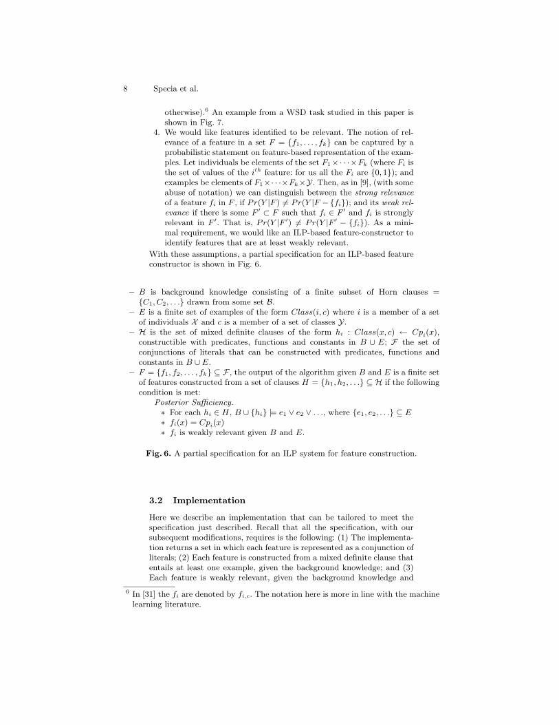
With these assumptions, a partial specification for an ILP-based featureconstructor is shown in Fig. 6.

– B is background knowledge consisting of a finite subset of Horn clauses ={C1, C2, . . .} drawn from some set B.

– E is a finite set of examples of the form Class(i, c) where i is a member of a setof individuals X and c is a member of a set of classes Y.

– H is the set of mixed definite clauses of the form hi : Class(x, c) ← Cpi(x),constructible with predicates, functions and constants in B ∪ E; F the set ofconjunctions of literals that can be constructed with predicates, functions andconstants in B ∪ E.

– F = {f1, f2, . . . , fk} ⊆ F , the output of the algorithm given B and E is a finite setof features constructed from a set of clauses H = {h1, h2, . . .} ⊆ H if the followingcondition is met:

Posterior Sufficiency.∗ For each hi ∈ H, B ∪ {hi} |= e1 ∨ e2 ∨ . . ., where {e1, e2, . . .} ⊆ E∗ fi(x) = Cpi(x)∗ fi is weakly relevant given B and E.

Fig. 6. A partial specification for an ILP system for feature construction.

3.2 Implementation

Here we describe an implementation that can be tailored to meet thespecification just described. Recall that all the specification, with oursubsequent modifications, requires is the following: (1) The implementa-tion returns a set in which each feature is represented as a conjunction ofliterals; (2) Each feature is constructed from a mixed definite clause thatentails at least one example, given the background knowledge; and (3)Each feature is weakly relevant, given the background knowledge and

6 In [31] the fi are denoted by fi,c. The notation here is more in line with the machinelearning literature.


Clause:h1 : Class(x, voltar)← Has expression(x, come back, voltar)

Has pos(x, pcwr 4, nn)

Context Predicate:Cp1(x) : Has expression(x, come back, voltar) ∧Has pos(x, pcwr 4, nn)

Feature:

f1(x) =

{1 Has expression(x, comeback, voltar) ∧Has pos(x, pcwr 4, n) = 1

0 otherwise

Fig. 7. Example of a boolean feature constructed from a clause for WSD. The clauseshown here identifies the Portuguese sense of the English verb “to come”. The meaningsof the predicate symbols Has expression and Has pos are explained in Section 4.

examples. Clearly a very large number of features can be constructedthat satisfy these requirements. Consequently, we introduce the follow-ing general constraints for restricting the number of features constructed:

Support. For each clause hi : Class(x, c)← Cpi(x) we compute P (hi) ={x : e ∈ E∧ e = Class(x, c)∧B∪{hi}∪{¬e} |= �}. P (hi) is the setof individuals correctly classified by hi, and we denote their num-ber by tp(hi) = |P (hi)| (more correctly of course, we should includeB and E in these functions). Adopting data-mining terminology, wecall this the “support” of a clause. In our implementation, we reducethe number acceptable clauses found by the ILP system (and hencethe number of features) by placing some minimal requirement on thesupport of any clause.

Precision. For each class c ∈ Y, we denote Nc = {¬Class(x, c) :Class(x, c′) ∈ E ∧ c 6= c′}. Then for each clause hi : Class(x, c) ←Cpi(x) we compute N(hi) = {x : e ∈ Nc ∧ e = ¬Class(x, c) ∧ B ∪{hi}∪{e} |= �}. N(hi) is the set of individuals incorrectly classifiedby a hi as class c, and we denote their number by fp(hi) = |N(hi)|.Once again, using terminology from the data-mining literature, weobtain the precision of a clause hi as the value tp(hi)/(tp(hi) +fp(hi)). In our implementation, we reduce the number acceptableclauses found by the ILP system (and hence the number of features)by requiring the precision of any clause to be greater than somepre-specified number.

We note that ensuring that the support of a clause is at least 1 meets therequirement that the clause entails at least one example. The constrainton precision can be used to ensure that features constructed are weaklyrelevant. This follows trivially, since each clause h for class c results in afeature f and the following contingency table for class values:

10 Specia et al.

Class

c c

1 tp(h) fp(h) na

f

0 Nc − tp(h) Nc − fp(h) nb

Nc Nc N

If the precision constraint ensures that the precision of a clause h fora class c is greater than the prior probability of class c (this probabil-ity is estimated from the examples E), then precision(h) = tp(h)/na >Nc/N = Pr(Class = c). Now, since Pr(Class = c|f = 1) = precision(h),it follows that Pr(Class|f) 6= Pr(Class). That is, the corresponding fea-ture f is weakly relevant.We will call any clauses (and, with some overloading of terminology, thecorresponding features) that satisfies the support and precision require-ments as “acceptable”. We distinguish between two different techniquesto obtain features:

1. One-shot feature-set construction, that identifies a set of acceptablefeatures without any feedback from the model constructor (this is,in some sense, a “LINUS-inspired” approach [14]). In keeping withterminology sometimes used in the ILP literature, we will call thisapproach “static feature-set construction”.

2. Incremental feature-set construction, that identifies a set of accept-able features after repeated iterations in which feature-constructionis guided by feedback from the model constructor. In keeping withterminology sometimes used in the ILP literature, we will call thisapproach “dynamic feature-set construction”.

We present these techniques as instances of the implementation below.

Randomised Feature-Set Construction

In [44] an implementation using a randomised local search was proposedto meet the specification of a predictive ILP system. It is possible toadopt the same approach in an implementation designed to meet thespecifications for feature construction (see Fig. 8).In Fig. 8 R and M bound the number of random restarts and localmoves allowed. Existing techniques for feature construction can be re-cast as special cases of this procedure, with appropriate values assignedto R and M ; and definitions of a starting point (Step 3a) and local moves(Step 3(f)i). For example, one-shot methods that use an ILP engine toconstruct a large number of features independent of the model construc-tor can be seen as an instance of the randomised procedure with R = 1and M = 0, with some technique for generating the “starting subset”


1. bestfeatures:= {}2. bestaccuracy:= 0.03. for i = 1 to R do begin

(a) currentfeatures:= randomly selected set of features(b) currentmodel:= model constructed with currentfeatures(c) accuracy:= estimated accuracy of currentmodel(d) if accuracy > bestaccuracy then begin

i. bestfeatures:= currentfeaturesii. bestaccuracy:= accuracy

(e) end(f) for j = 1 to M do begin

i. nextfeatures:= best local move from currentfeaturesii. nextmodel:= model constructed with nextfeaturesiii. accuracy:= estimated accuracy of nextmodeliv. if accuracy > bestaccuracy then begin

A. bestfeatures:= nextfeaturesB. bestaccuracy:= accuracy

v. endvi. currentfeatures:= nextfeatures

(g) end4. end5. return bestfeatures

Fig. 8. A basic randomised local search procedure, adapted to the task of feature construction.

in Step 3a. The feature-set constructor provided within the Aleph [39]system, shown in Fig. 9(a), is an example of a technique that generatesfeatures using a stratified sample of the examples (a simpler approachof generating k acceptable features using simple random sampling of theexamples is in Fig. 9(b)).

We consider now the more general procedure shown. In this, R and Mcan take on any value from the set of natural numbers (including 0). Inaddition, the starting subset is assumed to be drawn using some distri-bution that need not be known; and a local move is one that either addsa single new feature to the existing subset of features, or drops a featurefrom the existing subset. We are now immediately confronted with twoissues that make it impractical to use the procedure as shown. First, wehave the same difficulty that prevented us from using an enumerativetechnique like a Gibb’s sampler: generating the local neighbourhood re-quires us to obtain all possible single-feature additions. Second, for eachlocal move, we need to construct a model, which can often be computa-tionally expensive. We address each of these in turn.

Reducing Local Moves. We consider a modification of the search proce-dure in Fig. 8 that results in only examining a small sample of all thelocal moves possible before deciding on the next move in Step 3(f)i. Ide-ally, we are interested in obtaining a sample that, with high probability,contains the best local move possible. Assuming there are no ties, andthat the number of possible local moves is very large, it would clearly beundesirable to select the sample using a uniform distribution over localmoves. We propose instead a selection that uses the errors made by themodel-constructor to obtain a sample of local moves. As a result, featuresin the local neighbourhood that are relevant to the errors are more likelyto be selected. In some sense, this is somewhat reminiscent of boostingmethods: here, instead of increasing the weights of examples incorrectlyclassified, the representation language is enriched in a way that is biased

12 Specia et al.

strat features(B, E,Y, k, s, p,L) : Given background knowledge B; a set of examples E; a setof class-labels Y taken here to be the set of numbers {1, 2, . . . , c}; an upper-bound on thenumber of features allowed for each class k (1 ≤ k); the minimal support for acceptable clausess (1 ≤ s); the minimal precision for acceptable clauses p (0 < p ≤ 1); and a language Lspecifying constraints on acceptable clauses that can be considered in the search for any onefeature; return a set F of at most k acceptable features for each class.

1. for each i ∈ Y do2. begin

(a) Let Hi := ∅(b) Let Ei be all examples in E with class i(c) while (|Hi| ≤ k) and (Ei 6= ∅) do(d) begin

i. Randomly select an example e ∈ Ei

ii. Let j := k − |Hi|iii. Let H be a set of at most j mixed definite clauses found by an ILP engine such

that H ∩Hi = ∅, and each clause h ∈ H satisfies: (1) h ∈ L; (2) B ∪ {h} |= e; and(3) h is acceptable (that is, support(h) ≥ s; and precision(h) ≥ p).

iv. Let Hi := Hi ∪Hv. Let Ei := Ei − {e}

(e) end3. end4. Let F be the set of features obtained from the bodies of clauses in H1 ∪H2 · · ·Hc

5. return F

(a) A procedure for constructing a stratified sample of acceptable features.

srs features(B, E, k, s, p,L) : Given background knowledge B; a set of examples E; a set of class-labels Y taken here to be the set of numbers {1, 2, . . . , c}; an upper-bound on the number offeatures allowed k (1 ≤ k); the minimal support for acceptable clauses s (1 ≤ s); the minimalprecision for acceptable clauses p (0 < p ≤ 1); and a language L specifying constraints onacceptable clauses that can be considered in the search for any one feature; return a set F ofat most k acceptable features.

1. Let H = ∅2. Let E′ be a random subset of k examples from E3. while (|H| ≤ k) and (E′ 6= ∅) do4. begin

(a) Randomly select an example e ∈ E′

(b) Let j := k − |H|(c) Let H′ be a set of at most j mixed definite clauses found by an ILP engine such that

H ∩H′ = ∅, and each clause h ∈ H′ satisfies: (1) h ∈ L; (2) B ∪ {h} |= e; and (3) his acceptable (that is, support(h) ≥ s; and precision(h) ≥ p).

(d) Let H := H ∪H′

(e) Let E′ := E′ − {e}5. end6. Let F be the set of features obtained from the bodies of clauses in H7. return F

(b) A procedure for constructing a simple random sample of acceptable features.

Fig. 9. Candidates for using an ILP engine to generate the “starting subset” in therandomised search for features. support and precision are as described in the text.


to classify these examples correctly on subsequent iterations (the possi-bility of using misclassified examples to guide a stochastic local searchamongst an existing set of features was demonstrated in [25]).

Recall that at any point, a local move from a feature-subset F is obtainedby either dropping an existing feature in F or adding a new feature to F .We are specifically concerned with the addition step, since in principle,all possible features that can be constructed by the ILP engine could beconsidered as candidates. We curtail this in the following ways. First,we restrict ourselves to samples of features that are related to examplesmisclassifed by the model-constructor using the current set of featuresF (by “related” we mean those that are TRUE for at least one of theexamples in error). Second, in our implementation, we restrict ourselvesto a single new feature for each such example (by “new”, we mean afeature not already in F ).7

Reducing models constructed. The principal purpose of constructing andevaluating models in the local neighbourhood is to decide on the bestnext move to make. This will necessarily involve either an addition of anew feature to the existing set of features, or the deletion of an existingfeature from the current set of features. That is, we are looking to find thebest new feature to add, or the worst old feature to drop (given the otherfeatures in the set, of course). Correctly, we would form models with eachold feature omitted in turn from the current set and each new featureadded in turn to the current set. The best model would then determinethe next move. Using a model-constructor that assigns weights to featuresallows us to adopt the following sub-optimal procedure instead. First, wefind the feature with the lowest weight in the current model: this is takento be the worst old feature. Next, we construct a single model with allfeatures (old and new). Let us call this the “extended model”. The bestnew feature is taken to be the new feature with the highest weight in theextended model

The procedure in Fig. 8 with these modifications is shown in Fig. 10. Itis evident that the number of additional models constructed at any pointin the search space is now reduced to just 3: the price we pay is that weare not guaranteed to obtain the same result as actually performing theindividual additions and deletions of features.

It is the randomised local search procedure in Fig. 10, with one small dif-ference, that we implement in this paper. The difference arises from thecomparison of models: in the procedure shown, this is always done usingestimated accuracies only. In our implementation, if estimated accuraciesfor a pair of models are identical, then the model using fewer featuresis prefered (that is, comparisons are done on the pair (A,F ) where Ais the estimated accuracy of the model and F is the number of fea-tures used in the model). One additional point worth clarifying concernsover-fitting the data. Some combination of the following mechanisms areclearly possible: (a) Limiting the amount of local search (using M); (b)Requiring acceptable features have some reasonable support; and (c) Us-

7 In the implementation, we select this feature using its discriminatory power giventhe original set of examples.

14 Specia et al.

randsearch features(B, E,Y, n, s, pL, R, M) : Given background knowledge B; a set of examplesE; a set of class-labels Y taken here to be the set of numbers {1, 2, . . . , c}; a sample sizen (1 ≤ n); the minimal support for acceptable clauses s (1 ≤ s); the minimal precison foracceptable clauses p (0 < p ≤ 1); and a language L specifying constraints on acceptable clausesthat can be considered in the search for any one feature; the number of random restarts R(1 ≤ R); and the number of local moves M (1 ≤M), return a set of acceptable features F .

1. F :=2. bestaccuracy:= 0.03. for i = 1 to R do begin

(a) currentfeatures:= sample of acceptable features given B, E,Y, n, s, pL(b) currentmodel:= model constructed with currentfeatures(c) accuracy:= estimated accuracy of currentmodel(d) if accuracy > bestaccuracy then begin

i. F := currentfeaturesii. bestaccuracy:= accuracy

(e) end(f) for j = 1 to M do begin

i. Fnew:= sample of new acceptable features that are TRUE for errors made bycurrentmodel

ii. extendedmodel:= model constructed using currentfeatures and Fnew

iii. fworst:= feature in currentfeatures with lowest weight in currentmodeliv. fbest:= feature in Fnew with highest weight in extendedmodelv. F−:= set with feature subset obtained by dropping fworst from currentfeaturesvi. F+:= set with feature subset obtained by adding fbest to currentfeaturesvii. localmoves:= F− ∪ F+

viii. nextfeatures:= best subset in localmovesix. nextmodel:= model constructed with nextfeaturesx. accuracy:= estimated accuracy of nextmodelxi. if accuracy > bestaccuracy then begin

A. F := nextfeaturesB. bestaccuracy:= accuracy

xii. endxiii. currentfeatures:= nextfeaturesxiv. currentmodel:= nextmodel

(g) end4. end5. return F

Fig. 10. The randomised local search procedure for feature construction, modified using theory-guided sampling of local moves and the use of feature-weights to reduce model construction. Accept-able features are obtained using the same technique as the static feature-set constructor: an examplefor which the feature is required to be TRUE is selected, and then an acceptable clause found.

ing a model constructor that can perform some appropriate trade-off offit-versus-complexity to avoid over-fitting.We make the following observations about this implementation:

Termination. It is evident that, provided the ILP engine used constructfeatures terminates, the procedure in in Fig. 10 terminates, sinceboth R and M are finite.

Correctness. All features constructed are obtained from acceptableclauses. That is, the support of every clause is at least s (s > 1), and,precision is at least p. If p is ensured to be greater than the priorprobablity of any class c in the examples E, then from the discussionearlier, the corresponding features are all weakly relevant.

Incompleteness. The procedure does not identify all weakly relevantfeatures, since the local search procedure is incomplete.

Output. We assume that the starting subset in Step 3a contains fea-tures proportional to n (for example, with c classes, a starting subsetusing the Aleph feature-set constructor in Fig 9 will produce a setcontaining no more than cn features). On any restart, a local move


either adds a single feature to the existing set of features; or dropsa feature from this set. Since this done no more than M times, theoutput contains more than αn±M features (1 ≤ α <∞).

Based on the observations that: (a) the procedure in Fig. 10 terminates;and (b) with a value of p that can be determined from the examples,it returns a finite set of weakly relevant features, each constructed fromclauses that entail at least 1 example, we can view it as an algorithm forfeature construction.

4 Empirical Evaluation

Our objective is to evaluate empirically if ILP-based features can assistin constructing models for WSD. Specifically, given different sources ofbackground information, we intend to investigate the performance of thefollowing kinds of models:

Baseline models. These are models for WSD that use features thatare obtained manually from the different knowledge sources.

ILP-assisted models. These are models constructed by augmentingthe hand-crafted features with those found by either the static ordynamic feature-set construction techniques, when provided with ac-cess to a richer representation of the same background informationas the Baseline models. When static feature-set construction is used,we denote the resulting ILP-assisted model “ILP-S”; and when dy-namic feature-set construction is used, we denote the correspondingmodel “ILP-D”.

We wish to investigate whether the ILP-assisted models have a signif-icantly higher predictive accuracy than the baseline models. Statisticalevidence in favour of the ILP-assisted models will, in turn, be taken asproviding support for the “ILP-features hypothesis”, which we reiteratehere:

ILP-features hypothesis. Feature-construction by ILP pro-vides a general method of introducing background knowledgefor improving the predictive accuracy of WSD models.

Statistically speaking, the null hypothesis for the investigation is there isno difference in the (average) predictive accuracies of Baseline and ILP-S or ILP-D models. Inability to reject this hypothesis will be taken asevidence against the usefulness of ILP as a feature-constructor for WSD.

4.1 Materials

Data We experiment with datasets contained in three different tasks.Each collection is concerned with the disambiguation of different setsof ambiguous words, the so called “target words”, including nouns and

16 Specia et al.

verbs, and contain different numbers of classes (possible senses or trans-lations) and class distributions. The three tasks are:

Monolingual (1). Data consist of the 32 verbs from the SENSEVAL-3competition. SENSEVAL8 is a joint evaluation effort for WSD andrelated tasks. We use all the verbs of the English lexical sample taskfrom the third edition of the competition. The number of examplesfor each verb varies from 40 to 398 (average of 186). The number ofsenses varies from 3 to 12 with an average of 7 senses. The averageaccuracy of the majority class is about 55%. We refer the reader to[18] for more information about the SENSEVAL-3 data.

Monolingual(2). Data consist of 85 verbs and nouns of the Englishlexical sample task from the SemEval-2007 competition, the last edi-tion of SENSEVAL. The number of examples varies from 24 to 3,061(average of 272.12). The number of senses used in the training ex-amples for a given word varies from 1 to 13 (average of 3.6). The av-erage accuracy of the majority class is about 78%. More informationabout this data set can be found in [28].

Bilingual. Data consist of 7 highly frequent and ambiguous, mostlycontent-light, verbs: come, get, give, go, look, make, take. The sam-ple corpus comprises around 200 English sentences for each verbextracted from several corpora, including the European Parliament,the Bible and fiction books, with the verb translation automaticallyannotated [38]. The number of possible translations varies in thecorpus from 5 to 17, with an average of 11 translations. The averageaccuracy of the majority class in the test data is about 54%.

Taken together, the tasks specify 124 independent datasets, with dis-ambiguation required ranging from 3 to 17 different senses. The totalnumber of examples is approximately 27, 000.

Background Knowledge To achieve accurate disambiguation inboth tasks is believed to require a variety of lexical, syntactic and se-mantic information. In what follows, we describe the background knowl-edge available for the tasks and illustrate it using the following sentence(assuming that we are attempting to determine the sense of ‘coming’ astarget word):

“If there is such a thing as reincarnation, I would not mindcoming back as a squirrel.”

Background knowledge is available in the following categories:

B0. Baseline features. Manually identified features using the informa-tion encoded in the predicates below, conveying the same informa-tion, but represented by means of attribute-value vectors.

8 http://www.senseval.org


B1. Bag-of-words. The 5 words to the right and left of the target word,extracted from the corpus and represented using definitions of theform Has bag(sentence, word). For example:

Has bag(snt1,mind).Has bag(snt1, not). . . .

B2. Narrow context. Lemmas of 5 content words to the right and left ofthe target word, extracted from the corpus, previously lemmatizedby MINIPAR [16]. These are represented using definitions of theform Has narrow(sentence, wordposition,word). For example:

Has narrow(snt1, first content word left,mind).Has narrow(snt1, first content word right, back). . . .

These are not provided for the Bilingual task, since it was thoughtto be adeqately covered by B5 below.

B3. Part-of-speech tags. Part-of-speech (POS) tags of 5 content wordsto the right and left of the target word, are obtained using MX-POST [31] and represented using definitions of the form:Has pos(sentence, wordposition, pos). For example:

Has pos(snt1, first content word left, nn).Has pos(snt1, first content word right, rb). . . .

B4. Subject-Object relations. Subject and object syntactic relations withrespect to the target word - in case it is a verb. If it is a noun, therepresentation includes the verb of which it is a subject or object,and the verb / noun it modifies.These were obtained from parsingsentences using MINIPAR and represented using definitions of theform Has rel(sentence, type, word). For example:

Has rel(snt1, subject, i).Has rel(snt1, object, nil). . . .

B5. Word collocations. 11 collocations with respect to the target word,extracted from the corpus: 1st preposition to the right, 1st and 2ndwords to the left and right, 1st noun, 1st adjective, and 1st verb tothe left and right. These are represented using definitions of the formHas collocation(sentence, collocation type, collocation). For exam-ple:

Has collocation(snt1, first word right, back).Has collocation(snt1, first word left,mind). . . .

B6. Verb restrictions. Selectional restrictions of the verbs, when theseare the target words, defined in terms of the semantic features oftheir arguments in the sentence, extracted using LDOCE [29]. If therestrictions imposed by the verb are not part of the description of itsarguments, WordNet relations are used to check whether they canbe satisfied by synonyms or hyperonyms of those arguments. A hier-archy of feature types is used to account for restrictions establishedby the verb that are more generic than the features describing itsarguments in the sentence. These are represented by definitions ofthe form Satisfy restrictions(sentence, rest subject, rest object).For example:

Satisfy restrictions(snt1, [human], nil).Satisfy restrictions(snt1, [animal, human], nil).

18 Specia et al.

B7. Dictionary definitions. A relative count of the overlapping wordsin dictionary definitions of each of the possible senses of the targetword (extracted from [26], for the bilingual task, and from [29], forthe monolingual tasks) and the words surrounding it in the sen-tence, to find the sense with the highest number of overlappingwords. These are represented by facts of the form Has overlap(sentence, translation). For example:

Has overlap(snt1, voltar).B8. Phrasal verbs. Phrasal verbs involving the target verb, possibly oc-

curring in a sentence, according to the list of phrasal verbs given bydictionaries and the context of the verb (5 surrounding words). Theseare represented by definitions of the form Has expression(sentence,verbal expression). For example:

Has expression(snt1, ’come back’).This is not provided for Monolingual task (1) since it does not con-sider senses of the verbs occurring in phrasal verbs.

B9. Frequent bigrams. Bigrams consisting of pairs of adjacent wordsin a sentence (without the target word) which occur more than 10times in the corpus and are represented by definitions of the formHas bigram(sentence, word1, word2). For example:

Has bigram(snt1, such, a).Has bigram(snt1, back, as). . . .

These are available for Monolingual task (2) only.B10. Frequently related words. Related words consisting of pairs in the

sentence that occur in the corpus more than 10 times related by verb-subject, verb-object, verb-modifier, subject-modifier, and object-modifiersyntactic relations, without including the word to be disambiguated.There are represented by facts of the typeHas related pair(sentence,word1, word2). For example:

Has related pair(snt1, there, is). . . .These are available for Monolingual task (2) only.

Of these definitions, B0 is intended for constructing the Baseline model.B1–B10 are intended for use by an ILP system. For each task we used adifferent subset of these knowledge sources, according to their availabil-ity. Further, although the ILP implementation we use is entirely capableof exploring intensional definitions of each of B1–B10, we represent defi-nitions in an extensional form (that is, as a set of ground facts), since thisrepresentation is more efficient. This results in about 1.4 million facts.

Algorithms We distinguish here between three separate procedures:(1) The feature-construction algorithm in Fig. 10 for constructing a setof acceptable features; (2) The ILP engine concerned with identifyingclauses required by the feature-set construction algorithms; and (3) Theprocedure for constructing models given a set of features and their val-ues for sample instances, along with a class label associated with eachinstance. We have an implementation, in the Prolog language, of Fig. 10.For static-feature construction, the stratified sampling procedure pro-vided within the Aleph system shown in Fig. 9(a) is used to provide the“starting subset” of features. In other cases, we commence with a simple


random sample of features using the procedure in Fig. 9(b). For (2) weuse a basic branch-and-bound search procedure provided within Aleph,that attempts to find all clauses that satisfy a given set of constraintsand entail at least one example. The feature-based model constructor (3)is a linear SVM (the specific implementation used is the one providedin the WEKA toolbox called SMO.9). We will refer to (1) as “the fea-ture constructor”; (2) as “the ILP learner” and (3) as “the feature-basedlearner.”

4.2 Method

Our method is straightforward:

For each verb in each task (that is, 32 words in Monolingual(1), 85words in Monolingual(2) and 7 words in the Bilingual task):1. Obtain the best model possible using the feature-based learner

and the features in B0. Call this the Baseline model.2. Construct a set of features using, in turn, the static and dy-

namic feature construction that uses the ILP learner, equippedwith background knowledge definitions B1–B10. Call the corre-sponding sets of features “Static” and “Dynamic”.

3. Obtain the best model possible using the feature-based learnersupplied with data for features B0 ∪ Static. Call this model“ILP-S”. Similarly, obtain “ILP-D” using features B0 ∪ Dy-namic. For simplicity, we will refer to these models collectivelyas “ILP-assisted models”.

4. Compare the performance of the Baseline model against that ofthe ILP-assisted models.

The following details are relevant:

(a) For the monolingual tasks, we use the training/test data as providedby SENSEVAL-3 and SemEval-2007 benchmarks. These specify dif-ferent percentages for training and test, depending on the targetword. For the bilingual task, we use 25% of the data to estimate theperformance of disambiguation models. For all the data sets, per-formance is measured by the accuracy of prediction on the test set(that is, the percentage of test examples whose sense is predictedcorrectly).

(b) The ILP learner constructs a set of acceptable clauses in line withthe specifications described in Section 3.1. Positive examples for theILP learner are provided by the correct sense (or translation in thebilingual case) of the target word in a sentence. Negative examplesare generated automatically using all other senses (or translations).Clauses for a class are thus found using a “one-versus-the-rest” ap-proach.

(c) For each target word and task, constructing the “best possible model”requires determining optimal values for some parameters of the pro-cedures involved. We estimate these values using an instance of themethod proposed in [10] that proceeds as follows. First, we decide

9 http://www.cs.waikato.ac.nz/˜ml/weka/

20 Specia et al.

on the relevant parameters. Second, we obtain, using the training setonly, unbiased estimates of the predictive accuracy of the models foreach target word arising from systematic variation across some smallnumber of values for these parameters. Values that yielded the bestaverage predictive accuracy across all target words are taken to beoptimal ones. This procedure is not perfect: correctly, optimal valuesmay change from one target word to another; and even if they didnot, the results obtained may be a local maximum (that is, bettermodels may result from further informed variation of values).

(d) Full-scale experimentation for optimal settings for parameters re-quires systematic joint variation of values of critical parameters forthe feature constructor, ILP learner and the feature-based learner.For reasons of tractablility, we restrict this here to an exploration ofparameter values for the feature-based learner (here, a linear SVM)only. For the other two procedures, we select values that allow rea-sonably large numbers of features to be generated (see below). Theprincipal parameters for the feature-based learner are taken to be:the C parameter used by the linear SVM and F , the number offeatures to be selected. The following C values were investigated:0.1, 1.0, 10, 100, and 1000. Given a total of N features, F values con-sidered were N/64, N/32, N/16, N/8, N/4, N/2, and N (we obtainthe best subset of such features using software tools for feature-selection provided within WEKA). The predictive accuracy witheach (C,F ) setting is estimated and the values that yield the bestresults are used to construct the final model (the predictive accuracyestimate is obtained using an average over 5 repeats of predictionson 20% of the training data sampled to form a “validation” set).

(e) For the record, parameter settings for the feature-constructor andILP learner were as follows. For the former the value of k (the max-imum number of features constructed for each class) is 5000; theminimal support s required is 2; and the minimal precision 0.6. Wenote that this value of precision does always guarantee weak rele-vance in all datasets (where the prior probability of a class is > 0.6).In such cases, not all the features may be weakly relevant. In addi-tion, the search is bounded by requiring clauses to have no more than10 literals in the context-predicate (that is, the body of clauses hasat most 10 literals). Search for clauses is restricted to no more than10, 000 nodes. All these settings are admittedly ad hoc, with the in-tent being to place, within computational reason, as few constraintsas possible on feature generation.

(f) Comparison of performance is done using the Wilcoxon signed-ranktest [33]. This is a non-parametric test of the null hypothesis thatthere is no significant difference between the median performance ofa pair of algorithms. The test works by ranking the absolute valueof the differences observed in performance of the pair of algorithms.Ties are discarded and the ranks are then given signs depending onwhether the performance of the first algorithm is higher or lowerthan that of the second. If the null hypothesis holds, the sum ofthe signed ranks should be approximately 0. The probabilities ofobserving the actual signed rank sum can be obtained by an exact


calculation (if the number of entries is less than 10), or by using anormal approximation. We note that the comparing a pair of algo-rithms using the Wilcoxon test is equivalent to determining if thearea under the ROC curves of the algorithms differ significantly [?].

(g) We note also that given that the ILP-assisted models are constructedwith access to all features available for the Baseline model, we wouldexpect that the predictive accuracies of the ILP-assisted modelsshould, in principle, never be worse. That is, the alternate hypothesisfor the Wilcoxon test is a uni-directional one that the median accu-racy of the ILP-assisted model (ILP-S or ILP-D) is higher than theBaseline model. However, in practice, ILP-assisted models could beworse either due to overfitting, or due to limitations of the feature-selection procedure employed (if any). Given this, we adopt the bi-directional alternate hypothesis, that the median accuracies of theILP-assisted models are not equal to the Baseline model. This meansobtaining two-tailed probabilities for the signed rank-differences.

5 Results and Discussion

Figures 14, 15 and 16 in Appendix 6 tabulate the performance of theBaseline and ILP-assisted models on the three different WSD tasks. Itis also standard practice to include the performance of a classifier thatsimply predicts the most frequent sense of the target word, which wedenote in these tabulations as the “Majority class” model. The principaldetails in these tabulations are these: (1) The majority class classifierclearly performs poorest, and we will leave them out of any further dis-cussion; (2) For all three tasks, average accuracies of the baseline modelsare lower than the ILP-assisted models.We turn now to the question of whether the differences in accuracies ob-served between the Baseline and ILP-assisted models are in fact signifi-cant. The relevant probabilities calculated by using the Wilcoxon test areshown in Fig. 11.10 The tabulations show that, overall (see Fig. 11(a)),there is very little evidence in favour of the null hypothesis that themedian accuracies of the ILP-assisted models are the same as the Base-line model. Closer examination of the individual tasks (Fig. 11(b)–(d))suggests that we can be quite confident about this with ILP-D. ILP-S is also better, but some of the probabilities on Monolingual (1) andBilingual tasks are slightly lower than what would usually be consideredsignificant.These tabulations suggest that there is indeed evidence in favour of theILP-features conjecture, using ILP-S or ILP-D as an example of what isachievable with ILP assistance. One question of relevance to this conclu-sion is this: how do we know that the Baseline models are not deliber-ately poor? Clearly, we are not able to answer this question decisively.Nevertheless, setting aside the possibility of obtaining better models byusing a different feature-based learner, we provide some evidence that

10 These were obtained from the program kindly provided by Richard Lowry athttp://faculty.vassar.edu/lowry/wilcoxon.html.

22 Specia et al.

the hand-crafted features, although not provably the best possible, arenevertheless very good. A comparison of the Baseline models against thestate-of-the-art models reported for the Monolingual(1) dataset, shownin Fig. 12 below, suggests that these features yield models that are com-parable to the best available (without ILP assistance).11

Base ILP-S ILP-D

Base − − −ILP-S < 0.0001 − −ILP-D < 0.0001 < 0.0001 −

(a) Overall

Base ILP-S ILP-D Base ILP-S ILP-D Base ILP-S ILP-D

Base − − − Base − − − Base − − −ILP-S 0.06 − − ILP-S 0.0001 − − ILP-S 0.08 − −ILP-D 0.0006 0.002 − ILP-D < 0.0001 0.002 − ILP-D 0.02 > 0.10 −

(b) Monolingual (1) (c) Monolingual (2) (d) Bilingual

Fig. 11. Probablities of observing the differences in accuracies for the monolingual andbilingual tasks, under the null hypothesis that median accuracies of the pair of algo-rithms being compared are equal. Each entry consists two-tailed probability estimatesof the null hypothesis being true.

Finally, although not relevant to the principal hypothesis being investi-gated in the paper, but nevertheless of some interest for both automaticWSD and the ILP practitioner is the difference between static and dy-namic feature construction techniques embodied within ILP-S and ILP-D. On the evidence in the Appendix of this paper and Fig. 11, it ap-pears that, for WSD tasks at least, ILP-D is better (although resultsare not significantly better on the Bilingual subset). Besides their betterpredictive performance, ILP-D models also require substantially fewerfeatures—this is after the feature selection step—than ILP-S (and some-times even the baseline models: see Fig. 13), arising from the use of apartially correct model to direct the construction of only those featuresthat may be necessary to correct the model.

6 Concluding Remarks

Word sense disambiguation, a necessary component for a variety of natu-ral language processing tasks, remains amongst the hardest to model ade-quately. It is of course possible that the vagaries of natural language may

11 None of this, of course, address the question of whether features capturing some orall of the information found by the ILP learner could be hand-crafted. This is beyondthe scope of this paper.


Models Accuracy

MC-WSD [4] 72.50

Baseline 69.94

Syntalex-3 [20] 67.60

Syntalex-1 [20] 67.00

CLaC1 [12] 67.00

Syntalex-2 [20] 66.50

CLaC2 [12] 66.00

Syntalex-4 [20] 65.30

Majority class 55.31

Fig. 12. A comparison of the Baseline model against the best submissions made for theSENSEVAL-3 competition, that is, in the Monolingual (1) dataset. The best model,MC-WSD, is a multi-class averaged perceptron classifier with one component trainedon the data provided by SENSEVAL and on WordNet glosses.

Model Task

Monolingual (1) Monolingual (2) Bilingual

Baseline 136 282 102

ILP-S 2429 2813 2918

ILP-D 179 133 63

Fig. 13. Average numbers of features used by the different models.

place a limit on the accuracy with which a model could identify correctlythe sense of an ambiguous word, but it is not clear that this limit hasbeen reached with the modelling techniques that constitute the currentstate-of-the-art. The performance of these techniques depends largely onthe adequacy of the features used to represent the problem. As it stands,these features are usually hand-crafted and largely of a lexical nature.For substantial, scalable progress it is believed that knowledge that ac-counts for more elaborate syntactic and semantic information needs tobe incorporated. In this paper, we have investigated the use of InductiveLogic Programming as a mechanism for incorporating multiple sourcesof syntactic and semantic information into the construction of modelsfor WSD. The investigation has been in the form of empirical studies ofusing ILP to construct features that are then used to construct predictivemodels for monolingual and bilingual WSD tasks and the results provideevidence that this approach can yield better models.

We believe much of the gains observed with ILP stems from the use ofsubstantial amounts of background knowledge. For the work here, this

24 Specia et al.

knowledge has been obtained by translations of information in standardcorpora or electronic lexical resources. This is promising, as it suggeststhat these translators, in conjunction with ILP, may provide a set oftools for the automatic incorporation of deep knowledge into the con-struction of general WSD models. Turning specifically to the findings ofthis paper, a combination of randomised search and incremental feature-set construction by an ILP engine appears to be a promising method toconstruct good features for WSD.

There are a number of ways in which the work here can be improvedand extended. We list the main limitations here under three categories.On the conceptual front, it is evident that we have not provided anyguarantees of optimality on the feature-subset constructed. While this istypical of randomised methods of the type proposed here, it would nev-ertheless be useful to obtain some performance bounds, however loose.Our specification of a feature-construction algorithm—to the best of ourknowledge, the only one to be proposed in the ILP literature—can berefined to require the algorithm to return strongly relevant features (inthe sense described by [9]).

On the implementation front, our implementation of dynamic feature-setconstruction is based on the simplest kind of randomised search (GSAT).Better methods exist and need to be investigated (for example, WalkSat).Further, we could consider other neighbourhood definitions for the localsearch such as adding or dropping upto k features. Of course, we are notrestricted to use SVMs, or even the specific variant of SVM here, as ourmodel constructor. Our experiments on the monolingual tasks here sug-gest that there is no significant difference between a “1-norm” SVM andthe standard approach we have used here, but other model construc-tion techniques may yield better results. We note that the feature-setconstructor when used in conjunction with an SVM is an instance ofSVILP, as proposed in [23]. More generally, by interleaving feature andstatistical model construction in the dynamic feature-set constructor, weare effectively performing a form of statistical relational learning. Theapplicability of this approach to this wider area needs to be investigated.

On the application front, the background knowledge used here is by nomeans exhaustive of the kind available for the WSD tasks studied here.For example, for the bilingual task, the “translation context” for a targetword may help greatly. This refers to the translations into the target lan-guage of the words forming the context of the target word. Our prelimi-nary experiments show that this does improve accuracies on the bilingualtask. Further, the algorithms we have described here are unlikely to bethe only ones to satisfy the specifications for feature-constructors. Whilethe procedures in the paper establish a case for ILP-based feature con-struction in WSD, other feature-construction methods such as the onesin [13] and [6] may yield even better models, thus strengthening the casefor ILP further.

On the flip side, it is evident that the feature-construction algorithmwe have proposed here are not specific to WSD data. The use of thealgorithm to model data concerned with tasks other than WSD, whileoutside the scope of this paper, has obvious wider interest.


Acknowledgements

This work was begun when Lucia Specia visited Ashwin Srinivasan at theIBM Research Laboratory in New Delhi. Jimmy Foulds, at the Universityof Waikato, helped beyond the call of duty in getting an executableversion of code that constructed models using a 1-norm SVM withinWEKA.

References

1. Agirre, E. and Rigau, G.: Word Sense Disambiguation Using Con-ceptual Density. 16th International Conference on ComputationalLinguistics, Copenhagen 16–22 (1996)

2. Bar-Hillel, Y. Automatic Translation of Languages. In F. Alt, D.Booth, and R. E. Meagher (eds), Advances in Computers. AcademicPress, New York (1960)

3. Cannon, E.O., Amini, A., Bender, A., Sternberg, M.J.E., Muggle-ton S.H., Glen, R.C., Mitchell, J.B.O. Support vector inductive logicprogramming outperforms the naive Bayes classifier and inductivelogic programming for the classification of bioactive chemical com-pounds. J Comput Aided Mol Des, 21:269–280 (2007)

4. Ciaramita, M. and Johnson, M. Multi-component Word Sense Dis-ambiguation. SENSEVAL-3: 3rd International Workshop on theEvaluation of Systems for the Semantic Analysis of Text, Barcelona97–100 (2004)

5. Cottrell, G. W. A Connectionist Approach to Word Sense Disam-biguation. Research Notes in Artificial Intelligence. Morgan Kauf-mann, San Mateo (1989)

6. Davis, J., Ong, I., Struyf, J., Burnside, E., Page, D., and Costa, V.S.: Change of representation for statistical relational learning, Inter-national Joint Conferences on Artificial Intelligence, (2007) Hand,D.J.: Construction and Assessment of Classification Rules, JohnWiley, Chichester (1997).

7. Hirst, G. Semantic Intepretation and the Resolution of Ambigu-ity. Studies in Natural Language Processing. Cambridge UniversistyPress, Cambridge (1987)

8. Hovy, E.H., Marcus, M., Palmer, M., Pradhan, S., Ramshaw, L.,and Weischedel, R. OntoNotes: The 90% Solution. Human Lan-guage Technology / North American Association of ComputationalLinguistics conference, New York, 57–60 (2006)

9. John, G.H., Kohavi, R., Pfleger, K.: Irrelevant features and the sub-set selection problem, Proceedings of the Eleventh InternationalConference on Machine Learning, Morgan Kaufmann, 121–129,(1994)

10. Kohavi, R., and John, G.H. Automatic Parameter Selection by Min-imizing Estimated Error. 12th International Conference on MachineLearning, Morgan Kaufmann, San Francisco, CA (1995)

11. Kramer, S., Lavrac, N., and Flach, P. Propositionalization Ap-proaches to Relational Data Mining. Relational Data Mining, S.Dzeroski and N. Lavrac (eds), Springer 262–291 (2001)

26 Specia et al.

12. Lamjiri, A., Demerdash, O., Kosseim, F. Simple features for statis-tical Word Sense Disambiguation. SENSEVAL-3: 3rd InternationalWorkshop on the Evaluation of Systems for the Semantic Analysisof Text, Barcelona 133–136 (2004)

13. Landwehr, N., Passerini, A., Raedt, L. D., and Frasconi, P. kFOIL:Learning Simple Relational Kernels. In Gil, Y. and Mooney, R.,editors, Proc. Twenty-First National Conference on Artificial Intel-ligence (2006).

14. Lavrac, N., Dzeroski, S., and Grobelnik, M. Learning nonrecursivedefinitions of relations with LINUS. Technical report, Jozef StefanInstitute (1990)

15. Lesk, M. Automated Sense Disambiguation Using Machine-readableDictionaries: How to Tell a Pine Cone from an Ice Cream Cone.SIGDOC Conference, Toronto, 24–26 (1986)

16. Lin, D. Principle based parsing without overgeneration. 31st AnnualMeeting of the Association for Computational Linguistics, Colum-bus, 112–120 (1993)

17. McRoy, S. Using Multiple Knowledge Sources for Word Sense Dis-crimination. Computational Linguistics, 18(1):1–30 (1992)

18. Mihalcea, R., Chklovski, T., Kilgariff, A. The SENSEVAL-3 EnglishLexical Sample Task. SENSEVAL-3: 3rd International Workshop onthe Evaluation of Systems for Semantic Analysis of Text, Barcelona25–28 (2004)

19. Miller, G.A., Beckwith, R.T., Fellbaum, C.D., Gross, D., Miller,K. Wordnet: An On-line Lexical Database. International Journal ofLexicography, 3(4):235–244 (1990)

20. Mohammad, S. and Pedersen, T. Complementarity of Lexical andSimple Syntactic Features: The SyntaLex Approach to SENSEVAL-3. SENSEVAL-3: 3rd International Workshop on the Evaluationof Systems for the Semantic Analysis of Text, Barcelona, 159–162(2004)

21. Muggleton, S. Inductive Logic Programming: derivations, successesand shortcomings. SIGART Bulletin 5(1):5–11 (1994)

22. Muggleton, S. and Raedt, L. D. Inductive logic programming: The-ory and methods. Journal of Logic Programming 19,20:629–679(1994)

23. Muggleton,S., Lodhi,H., Amini,A., Sternberg,M.J.E.: Support vec-tor inductive logic programming, 8th International Conference onDiscovery Science, Springer-Verlag, 163–175, (2005)

24. Nienhuys-Cheng, S. and de Wolf, R. Foundations of Inductive LogicProgramming. Springer, Berlin (1997)

25. Paes, A., Zaverucha, G., Page, C.D. Jr., and Srinivasan, A.: ILPthrough propositionalization and stochastic k-term DNF learning.Sense Disambiguation using Inductive Logic Programming. Selectedpapers from the 16th International Conference on Inductive LogicProgramming, LNCS 4455, Springer-Verlag, 379–393 (2007)

26. Parker, J.; Stahel, M. Password: English Dictionary for Speakers ofPortuguese. Martins Fontes, Sao Paulo (1998)

27. Pedersen, T. A Baseline Methodology for Word Sense Disambigua-tion. 3rd International Conference on Intelligent Text Processingand Computational Linguistics, Mexico City (2002)


28. Pradhan, S., Loper, E., Dligach, D. and Palmer, M. SemEval-2007Task-17: English Lexical Sample, SRL and All Words. Fourth Inter-national Workshop on Semantic Evaluations, Prague, 87–92 (2007)

29. Procter, P. (editor). Longman Dictionary of Contemporary English.Longman Group, Essex (1978)

30. Quillian, M.R. A Design for an Understanding Machine. Colloquiumof semantic problems in natural language. Cambridge University,Cambridge (1961)

31. Ratnaparkhi, A. A Maximum Entropy Part-Of-Speech Tagger. Em-pirical Methods in NLP Conference, University of Pennsylvania(1996)

32. Schutze, H. Automatic Word Sense Discrimination. ComputationalLinguistics, 24(1):97–124 (1998)

33. Siegel, S. Nonparametric Statistics for the Behavioural Sciences.McGraw-Hill, New York (1956)

34. Specia, L.: A Hybrid Relational Approach for WSD - First Results.Student Research Workshop at Coling-ACL, Sydney, 55–60, (2006)

35. Specia, L., Nunes, M.G.V., Stevenson, M. Learning Expressive Mod-els for Word Sense Disambiguation. 45th Annual Meeting of theAssociation for Computational Linguistics, Prague, 41–48 (2007)

36. Specia, L., Nunes, M.G.V., Srinivasan, A., Ramakrishnan, G. WordSense Disambiguation using Inductive Logic Programming. Selectedpapers from the 16th International Conference on Inductive LogicProgramming, LNCS 4455, Springer-Verlag, 409–423 (2007)

37. Specia, L., Nunes, M.G.V., Srinivasan, A., Ramakrishnan, G. USP-IBM-1 and USP-IBM-2: The ILP-based Systems for Lexical SampleWSD in SemEval-2007. 4th International Workshop on SemanticEvaluations, Prague, 442–445 (2007)

38. Specia, L, Nunes, M.G.V., and Stevenson, M. Exploiting ParallelTexts to Produce a Multilingual Sense-tagged Corpus for WordSense Disambiguation. RANLP-05, Borovets, 525–531 (2005)

39. Srinivasan, A. The Aleph Manual. Available athttp://www.comlab.ox.ac.uk/oucl/research/areas/machlearn/Aleph/ (1999)

40. Stevenson, M. and Wilks, Y. The Interaction of KnowledgeSources for Word Sense Disambiguation. Computational Linguis-tics, 27(3):321–349 (2001)

41. Wilks, Y. and Stevenson, M. Combining Independent KnowledgeSources for Word Sense Disambiguation. 3rd Conference on Re-cent Advances in Natural Language Processing, Tzigov Chark, 1–7(1997)

42. Wilks, Y. and Stevenson, M. The Grammar of Sense: Using Part-of-speech Tags as a First Step in Semantic Disambiguation. NaturalLanguage Engineering, 4(1):1–9 (1998)

43. Yarowsky, D. Unsupervised Word Sense Disambiguation RivalingSupervised Methods. 33rd Annual Meeting of the Association forComputational Linguistics, Cambridge, 189–196 (1995)

44. Zelezny, F., Srinivasan, A., and Page C.D. Jr.: Randomised restartedsearch in ILP. Machine Learning 64(1-3): 183-208 (2006)

28 Specia et al.

A Tabulation of Results

Word Majority Class Baseline ILP-S ILP-Dactivate 82.46± 3.56 81.58± 3.63 82.45± 3.56 92.98± 2.39add 45.80± 4.35 81.68± 3.38 83.21± 3.27 85.50± 3.08appear 44.70± 4.33 70.45± 3.97 71.21± 3.94 88.64± 2.76ask 27.78± 3.99 53.97± 4.44 53.17± 4.45 60.32± 4.36begin 59.74± 5.59 63.64± 5.48 72.73± 5.08 74.03± 5.00climb 55.22± 6.08 71.64± 5.51 86.57± 4.17 85.07± 4.35decide 67.74± 5.94 79.03± 5.17 80.64± 5.02 79.03± 5.17eat 88.37± 3.46 87.21± 3.60 88.37± 3.46 87.21± 3.60encounter 50.77± 6.20 73.85± 5.45 72.30± 5.55 73.85± 5.45expect 74.36± 4.94 79.49± 4.57 92.31± 3.02 92.31± 3.02express 69.09± 6.23 67.27± 6.33 67.27± 6.33 78.18± 5.57hear 46.88± 8.82 62.50± 8.56 62.50± 8.56 65.63± 8.40lose 52.78± 8.32 52.78± 8.32 52.70± 8.32 52.78± 8.32mean 52.50± 7.90 72.50± 7.06 75.00± 6.85 75.00± 6.85miss 33.33± 8.61 36.67± 8.80 36.66± 8.80 40.00± 8.94note 38.81± 5.95 53.73± 6.09 88.06± 3.96 88.06± 3.96operate 16.67± 8.78 66.67± 11.11 72.22± 10.56 72.22± 10.56play 46.15± 6.91 53.85± 6.91 55.77± 6.89 55.77± 6.89produce 52.13± 5.15 63.83± 4.96 65.96± 4.89 74.47± 4.50provide 85.51± 4.24 89.86± 3.63 86.96± 4.05 89.86± 3.63receive 88.89± 6.05 88.89± 6.05 88.89± 6.05 88.89± 6.05remain 78.57± 4.90 84.29± 4.35 85.71± 4.18 87.14± 4.00rule 50.00± 9.13 66.67± 8.61 83.33± 6.80 86.67± 6.21smell 40.74± 6.69 79.63± 5.48 75.92± 5.82 74.07± 5.96suspend 35.94± 6.00 56.25± 6.20 56.25± 6.20 57.81± 6.17talk 72.60± 5.22 73.97± 5.14 73.97± 5.14 73.97± 5.14treat 28.07± 5.95 47.37± 6.61 57.89± 6.54 50.88± 6.62use 71.43± 12.07 92.86± 6.88 92.86± 6.88 92.86± 6.88wash 67.65± 8.02 73.53± 7.57 61.76± 8.33 64.71± 8.20watch 74.51± 6.10 76.47± 5.94 72.54± 6.25 74.51± 6.10win 44.74± 8.07 47.37± 8.10 57.89± 8.01 60.53± 7.93write 26.09± 9.16 47.83± 10.42 39.13± 10.18 52.17± 10.42

Micro 56.26± 1.12 69.94± 1.03 73.14± 1.00 76.60± 0.95Macro 55.31± 1.12 68.67± 1.05 71.63± 1.02 74.22± 0.99

Fig. 14. Estimates of accuracies of disambiguation models for datasets in Monolingual(1) task. “Micro” and “Macro” refer to averages weighted, and un-weighted by thenumber of examples.


Word Majority Class Baseline ILP-S ILP-D

allow 97.14 ± 2.82 97.14 ± 2.82 97.14 ± 2.82 100.00 ± 0.00announce 100.00 ± 0.00 100.00 ± 0.00 100.00 ± 0.00 100.00 ± 0.00approve 91.67 ± 7.98 91.67 ± 7.98 91.67 ± 7.98 91.67 ± 7.98area 70.27 ± 7.51 62.16 ± 7.97 62.16 ± 7.97 62.16 ± 7.97ask 51.72 ± 6.56 50.00 ± 6.57 94.83 ± 2.91 94.83 ± 2.91authority 23.81 ± 9.29 47.62 ± 10.90 57.14 ± 10.80 90.48 ± 6.41base 10.00 ± 6.71 30.00 ± 10.25 35.00 ± 10.67 30.00 ± 10.25begin 56.25 ± 7.16 45.83 ± 7.19 33.33 ± 6.80 35.42 ± 6.90believe 78.18 ± 5.57 67.27 ± 6.33 100.00 ± 0.00 100.00 ± 0.00bill 75.49 ± 4.26 66.67 ± 4.67 64.71 ± 4.73 64.71 ± 4.73build 73.91 ± 6.47 60.87 ± 7.20 56.52 ± 7.31 69.57 ± 6.78buy 76.09 ± 6.29 69.57 ± 6.78 91.30 ± 4.15 91.30 ± 4.15capital 96.49 ± 2.44 96.49 ± 2.44 96.49 ± 2.44 98.25 ± 1.74care 28.57 ± 17.07 42.86 ± 18.70 42.86 ± 18.70 42.86 ± 18.70carrier 71.43 ± 9.86 71.43 ± 9.86 71.43 ± 9.86 71.43 ± 9.86chance 40.00 ± 12.65 20.00 ± 10.33 20.00 ± 10.33 20.00 ± 10.33claim 80.00 ± 10.33 80.00 ± 10.33 80.00 ± 10.33 80.00 ± 10.33come 23.26 ± 6.44 20.93 ± 6.20 20.93 ± 6.20 20.93 ± 6.20complain 85.71 ± 9.35 85.71 ± 9.35 85.71 ± 9.35 85.71 ± 9.35complete 93.75 ± 6.05 93.75 ± 6.05 93.75 ± 6.05 93.75 ± 6.05condition 76.47 ± 7.27 73.53 ± 7.57 79.41 ± 6.93 100.00 ± 0.00contribute 50.00 ± 11.79 38.89 ± 11.49 50.00 ± 11.79 100.00 ± 0.00defense 28.57 ± 9.86 14.29 ± 7.64 19.05 ± 8.57 14.29 ± 7.64describe 100.00 ± 0.00 100.00 ± 0.00 100.00 ± 0.00 100.00 ± 0.00development 62.07 ± 9.01 62.07 ± 9.01 58.62 ± 9.15 58.62 ± 9.15do 90.16 ± 3.81 90.16 ± 3.81 90.16 ± 3.81 100.00 ± 0.00drug 86.96 ± 4.97 76.09 ± 6.29 69.57 ± 6.78 71.74 ± 6.64effect 76.67 ± 7.72 63.33 ± 8.80 60.00 ± 8.94 60.00 ± 8.94end 52.38 ± 10.90 47.62 ± 10.90 47.62 ± 10.90 52.38 ± 10.90enjoy 57.14 ± 13.23 50.00 ± 13.36 57.14 ± 13.23 50.00 ± 13.36examine 100.00 ± 0.00 100.00 ± 0.00 100.00 ± 0.00 100.00 ± 0.00exchange 73.77 ± 5.63 63.93 ± 6.15 63.93 ± 6.15 63.93 ± 6.15exist 100.00 ± 0.00 100.00 ± 0.00 100.00 ± 0.00 100.00 ± 0.00explain 88.89 ± 7.41 88.89 ± 7.41 83.33 ± 8.78 83.33 ± 8.78feel 68.63 ± 6.50 68.63 ± 6.50 100.00 ± 0.00 100.00 ± 0.00find 82.14 ± 7.24 78.57 ± 7.75 82.14 ± 7.24 85.71 ± 6.61future 86.30 ± 2.85 77.40 ± 3.46 85.62 ± 2.90 92.47 ± 2.18go 45.90 ± 6.38 32.79 ± 6.01 37.70 ± 6.21 39.34 ± 6.25grant 80.00 ± 17.89 80.00 ± 17.89 100.00 ± 0.00 100.00 ± 0.00hold 37.50 ± 9.88 25.00 ± 8.84 54.17 ± 10.17 83.33 ± 7.61hour 89.58 ± 4.41 85.42 ± 5.09 89.58 ± 4.41 75.00 ± 6.25job 82.05 ± 6.15 76.92 ± 6.75 97.44 ± 2.53 97.44 ± 2.53join 38.89 ± 11.49 38.89 ± 11.49 55.56 ± 11.71 100.00 ± 0.00keep 56.25 ± 5.55 46.25 ± 5.57 75.00 ± 4.84 92.50 ± 2.94kill 87.50 ± 8.27 87.50 ± 8.27 87.50 ± 8.27 87.50 ± 8.27lead 38.46 ± 7.79 30.77 ± 7.39 43.59 ± 7.94 97.44 ± 2.53maintain 90.00 ± 9.49 80.00 ± 12.65 80.00 ± 12.65 80.00 ± 12.65management 71.11 ± 6.76 62.22 ± 7.23 57.78 ± 7.36 60.00 ± 7.30move 97.87 ± 2.10 97.87 ± 2.10 97.87 ± 2.10 97.87 ± 2.10need 71.43 ± 6.04 57.14 ± 6.61 57.14 ± 6.61 58.93 ± 6.57network 90.91 ± 3.88 76.36 ± 5.73 78.18 ± 5.57 74.55 ± 5.87occur 86.36 ± 7.32 77.27 ± 8.93 77.27 ± 8.93 95.45 ± 4.44order 91.23 ± 3.75 91.23 ± 3.75 96.49 ± 2.44 96.49 ± 2.44part 66.20 ± 5.61 50.70 ± 5.93 95.77 ± 2.39 97.18 ± 1.96people 90.43 ± 2.74 86.09 ± 3.23 100.00 ± 0.00 100.00 ± 0.00plant 98.44 ± 1.55 98.44 ± 1.55 98.44 ± 1.55 96.88 ± 2.17point 81.33 ± 3.18 70.00 ± 3.74 78.00 ± 3.38 89.33 ± 2.52policy 97.44 ± 2.53 97.44 ± 2.53 100.00 ± 0.00 100.00 ± 0.00position 46.67 ± 7.44 28.89 ± 6.76 91.11 ± 4.24 91.11 ± 4.24power 27.66 ± 6.52 53.19 ± 7.28 53.19 ± 7.28 55.32 ± 7.25prepare 77.78 ± 9.80 55.56 ± 11.71 61.11 ± 11.49 66.67 ± 11.11president 72.88 ± 3.34 68.36 ± 3.50 68.36 ± 3.50 67.80 ± 3.51produce 75.00 ± 6.53 72.73 ± 6.71 95.45 ± 3.14 95.45 ± 3.14promise 75.00 ± 15.31 75.00 ± 15.31 62.50 ± 17.12 75.00 ± 15.31propose 85.71 ± 9.35 85.71 ± 9.35 85.71 ± 9.35 85.71 ± 9.35prove 68.18 ± 9.93 45.45 ± 10.62 50.00 ± 10.66 45.45 ± 10.62raise 14.71 ± 6.07 8.82 ± 4.86 8.82 ± 4.86 20.59 ± 6.93rate 86.21 ± 2.86 79.31 ± 3.36 100.00 ± 0.00 100.00 ± 0.00recall 86.67 ± 8.78 86.67 ± 8.78 86.67 ± 8.78 86.67 ± 8.78receive 95.83 ± 2.88 95.83 ± 2.88 93.75 ± 3.49 95.83 ± 2.88regard 71.43 ± 12.07 78.57 ± 10.97 71.43 ± 12.07 78.57 ± 10.97remember 100.00 ± 0.00 100.00 ± 0.00 100.00 ± 0.00 100.00 ± 0.00replace 100.00 ± 0.00 100.00 ± 0.00 100.00 ± 0.00 100.00 ± 0.00report 91.43 ± 4.73 91.43 ± 4.73 91.43 ± 4.73 91.43 ± 4.73rush 100.00 ± 0.00 100.00 ± 0.00 100.00 ± 0.00 100.00 ± 0.00say 98.71 ± 0.49 98.52 ± 0.52 99.63 ± 0.26 99.63 ± 0.26see 44.44 ± 6.76 37.04 ± 6.57 40.74 ± 6.69 35.19 ± 6.50set 28.57 ± 6.97 19.05 ± 6.06 19.05 ± 6.06 21.43 ± 6.33share 97.14 ± 0.73 95.62 ± 0.89 98.10 ± 0.60 98.10 ± 0.60source 37.14 ± 8.17 25.71 ± 7.39 22.86 ± 7.10 25.71 ± 7.39space 78.57 ± 10.97 92.86 ± 6.88 78.57 ± 10.97 78.57 ± 10.97system 48.57 ± 5.97 40.00 ± 5.86 98.57 ± 1.42 98.57 ± 1.42turn 38.71 ± 6.19 22.58 ± 5.31 27.42 ± 5.67 22.58 ± 5.31value 98.31 ± 1.68 94.92 ± 2.86 100.00 ± 0.00 100.00 ± 0.00work 55.81 ± 7.57 46.51 ± 7.61 48.84 ± 7.62 48.84 ± 7.62

Micro 78.10 ± 0.62 73.41 ± 0.66 80.58 ± 0.59 83.15 ± 0.56Macro 71.69 ± 0.67 67.53 ± 0.70 73.56 ± 0.66 77.40 ± 0.62

Fig. 15. Estimates of accuracies of disambiguation models for datasets in Monolingual(2) task.

30 Specia et al.

Word Majority Class Baseline ILP-S ILP-Dcome 50.30± 7.45 60.00± 7.30 75.56± 6.41 75.56± 6.41get 21.00± 6.52 30.77± 7.39 64.10± 7.68 76.92± 6.75give 88.80± 4.70 95.56± 3.07 100.00± 0.00 100.00± 0.00go 68.50± 6.64 73.47± 6.31 77.55± 5.96 75.51± 6.14look 50.30± 7.29 78.72± 5.97 76.59± 6.18 80.85± 5.74make 70.00± 7.07 78.57± 6.33 78.57± 6.33 90.48± 4.53take 28.50± 7.98 43.75± 8.77 56.25± 8.77 53.13± 8.82

Micro 55.69± 2.87 67.56± 2.71 76.59± 2.45 79.93± 2.32Macro 53.91± 2.88 65.83± 2.74 75.52± 2.49 78.92± 2.36

Fig. 16. Estimates of accuracies of disambiguation models for datasets in the bilingualtask.

an investigation into feature construction to assist …ganesh/papers/mlj08-accepted.pdfan...

Documents