an investigation into the potential impacts of farming … investigation into the potential impacts...
TRANSCRIPT

1
An investigation into the potential impacts of
farming practices on Loweswater
Stephen Maberly1, Lisa Norton1, Linda May2, Mitzi De Ville1, Alex Elliott1, Steve
Thackeray1, Rene Groben1 and Fiona Carse1
Centre for Ecology & Hydrology
1. Lancaster Environment Centre, Library Avenue, Bailrigg, Lancaster, LA1 4AP UK
2. CEH Edinburgh, Bush Estate, Penicuik, Midlothian, Edinburgh EH26 0QB
A report to the Rural Development Service and the National Trust (funded through the Rural Enterprise Scheme)
January 2006
Report Number: LA/C02707/4

2
Executive Summary
1. Loweswater is a small lake on the north-west edge of the Lake District National Park lying in a largely agricultural catchment. The catchment is managed by 13 land-owners, including the National Trust, mainly under the Environmentally Sensitive Area (ESA) scheme. Beef cattle and sheep production are the major farming activities. There are also facilities for tourism in the form of a small hotel, a camping barn and bothy, self-catering accommodation and some letting of rooms as well as boat hire and the sale of fishing permits for use on the lake.
2. There is evidence of decreasing water quality in Loweswater, partly manifested as an increase in algal bloom frequency and intensity. There is a concern that this may have resulted from changes in the management of the farms within the catchment, particularly with respect to the intensity of cattle farming and the application of fertiliser. This led the local farmers to band together to form the ‘Loweswater Improvement Project’ to investigate ways of minimising their impact on the lake. The aim of this report is to provide scientific evidence on how the lake functions and responds to nutrients from the catchment to allow sound management of the lake.
3. A monthly study of Loweswater was undertaken from October 2004 to September 2005. In Loweswater, like most lowland lakes, phytoplankton production is controlled by the availability of phosphorus. The concentration of soluble reactive phosphorus, which equates to the form available to phytoplankton, is very low throughout summer. Silica and nitrate were not depleted to concentrations that would limit availability to the phytoplankton during this study period. The phytoplankton produced a spring bloom dominated by cyanobacteria (blue-green algae), mainly Planktothrix mougeotii. This contrasts with the normal pattern of diatom dominance in the spring that is found in many other lakes: the difference is probably caused by the relatively long retention time of the lake which allows slow-growing filamentous cyanobacteria to dominate. The high lake productivity causes substantial oxygen depletion at depth. This may allow phosphorus stored in the sediment to be released into the water and become available to the phytoplankton. The smaller summer phytoplankton bloom is probably largely supported by internal cycling of nutrients aided by phosphate release from the sediments.
4. Long-term changes in Loweswater were assessed largely from ‘Lakes Tour’ samples taken four-times a year in 1984, 1991, 1994, 2000 and 2005. The data provide clear and consistent evidence of increased lake productivity caused by increased supply of phosphorus to the lake. There has been a statistically significant increase in total phosphorus both in spring and as an average over the whole year. In response, concentrations of phytoplankton in spring and as an annual mean have also increased (albeit not quite statistically significantly) and this is likely to be linked to a decline in water transparency. A decline in concentrations of nitrate in summer and autumn but not in winter and spring is also likely to result from greater availability of phosphorus which causes increased demand for nitrate. Increased productivity has led to a significant decline in oxygen concentration at depth and the bottom water of Loweswater is now anoxic in summer which probably results in release of more phosphate into the water column.
5. Paleolimnological records and an approach based on lake morphometry and alkalinity results in an estimate of 10 mg m-3 for historical concentrations of total phosphorus in Loweswater. This compares with a 12-month mean today of 14.5 mg m-3. This is slightly lower than the mean in 2000 of 16.5 mg m-3 which gives slight hope that the trend towards increasing levels in recent years may now have halted. This possible

3
improvement is also apparent in the January concentrations of soluble reactive phosphorus and the spring concentrations of phytoplankton chlorophyll a.
6. Assessment of the trophic state of Loweswater, based on a number of features, suggests that over the last 20 years it has changed from mesotrophic to meso-eutrophic. The ecological status of Loweswater, based on current ecological boundaries, suggests that the lake is at moderate status for phytoplankton chlorophyll a concentration and just in the good category for total phosphorus concentration. There is likely, therefore, to be a legal requirement to improve the ecological status of Loweswater by 2015 under the EC Water Framework Directive.
7. Nutrient loads to the lake were estimated in a number of ways: direct measurement, export coefficient modelling and Generalised Watershed Loading Functions modelling. The catchment, without major inputs from animal or human waste, delivers about 168 kg TP y-1 and 37 kg SRP y-1. This is mainly derived from the improved grassland within the catchment which contributes 62% of the TP load even though it only occupied 35% of the catchment area, presumably at least in part as a result of fertiliser application.
8. Activities related to animal husbandry, including spreading manure and run-off from farmyards contributed an additional 52 kg P y-1 and septic tanks, if functioning correctly, will contribute a further 23 kg P y-1. However, as a worse case scenario, if all the septic tanks were malfunctioning they would contribute 96 kg TP y-1. Thus the estimate of the current TP load to Loweswater ranges from 243 to 316 kg TP y-1 depending on whether or not the septic tanks are functioning properly. The equivalent SRP loads are from 113 to 183 kg SRP y-1.
9. PROTECH simulations confirmed the dominant effect of phosphorus in controlling phytoplankton production. The highest priority management approach in terms of magnitude of effect and practicality is to ensure that all of the septic tanks are functioning correctly as this has the largest effect on the crop of phytoplankton produced in the lake. The second priority would be to reduce losses of phosphorus from animal husbandry activities- for example by restricting slurry spreading and by reducing input from slurry tanks. However, the catchment, especially the improved grassland, is a major source of phosphorus. Current attempts to reduce phosphorus inputs by reducing P-application in fertilisers are to be encouraged. The speed of any recovery from this is hard to predict and will depend on delivery pathways in the catchment and the extent of internal recycling of phosphorus within the lake.
10. A continued low-level monitoring programme is recommended to continue using the Lakes Tour format supplemented by an additional mid-August sample, in order to evaluate the effectiveness of the changes that are being implemented in the catchment to improve water quality.

4
Table of contents
1. Introduction and background..........................................................................................6 2. Limnological survey of Loweswater over 12-months ..................................................10 2.1 Introduction....................................................................................................................10 2.2 Methods .........................................................................................................................10 2.2.1 Oxygen and temperature profiles of the water column..............................................10 2.2.2 Secchi disc transparency............................................................................................10 2.2.3 Water samples ............................................................................................................10 2.2.4 Nutrient and chemical analysis..................................................................................11 2.2.5 Algal pigments and populations.................................................................................11 2.3 Results............................................................................................................................11 2.3.1 Temperature and stratification ..................................................................................11 2.3.2 Oxygen concentration ................................................................................................13 2.3.3 pH and alkalinity........................................................................................................14 2.3.4 Nutrients.....................................................................................................................15 2.3.5 Chlorophyll a and Secchi depth.................................................................................16 2.3.6 Phytoplankton composition........................................................................................17 2.4 Discussion......................................................................................................................19 3. Changes in water quality in Loweswater using historic and contemporary data.....21 3.1 Introduction....................................................................................................................21 3.2 Materials & Methods .....................................................................................................21 3.3 Results............................................................................................................................22 3.3.1 Alkalinity....................................................................................................................22 3.3.2 Total Phosphorus .......................................................................................................23 3.3.3 Soluble Reactive Phosphorus.....................................................................................25 3.3.4 Nitrate........................................................................................................................26 3.3.5 Silica...........................................................................................................................27 3.3.6 Phytoplankton chlorophyll a and Secchi depth .........................................................28 3.3.7 Oxygen concentration at depth..................................................................................30 3.4 Discussion and Conclusions ..........................................................................................31 4. Assessment of nutrient load to the lake.........................................................................35 4.1 Nutrients loads from direct measurement ......................................................................35 4.1.1 Introduction................................................................................................................35 4.1.2 Methods......................................................................................................................36 4.1.3 Results........................................................................................................................37 4.2 Survey of streams for high concentrations of phosphate ...............................................45 4.2.1 Introduction................................................................................................................45 4.2.2 Methods......................................................................................................................45 4.2.3 Results & Discussion .................................................................................................45 4.3 Release of nutrients to streams as a result of farm management events........................47 4.3.1 Introduction................................................................................................................47 4.3.2 Methods......................................................................................................................47 4.3.3 Results........................................................................................................................48 4.3.4 Discussion ..................................................................................................................49 4.4 Total phosphorus load derived from export coefficients ...............................................49 4.4.1 Introduction................................................................................................................49 4.4.2 Methods......................................................................................................................50

5
4.4.3 Results........................................................................................................................53 4.5 Loads of SRP based on a calibrated nutrient runoff model...........................................55 4.5.1 Introduction................................................................................................................55 4.5.2 Methods......................................................................................................................57 4.5.3 Results........................................................................................................................60 4.6 Discussion......................................................................................................................61 5. Lake modelling of scenarios of phosphorus loading to Loweswater..........................62 5.1 Introduction....................................................................................................................62 5.2 Calibration and validation..............................................................................................63 5.3 Modelled scenarios ........................................................................................................67 5.4 Discussion......................................................................................................................69 6. Summary and Conclusions .............................................................................................70 7. Acknowledgements .........................................................................................................72 8. References........................................................................................................................73 9. Appendices.......................................................................................................................77

6
1. Introduction and background
Loweswater is a small lake on the north-west edge of the Lake District National Park and the
only major lake that flows into the centre of the Lake District. The main geographical and
physical features of Loweswater are shown in Table 1.1. In comparison to the other major
nineteen lakes in the English Lake District, Loweswater is the 13th smallest in terms of lake
area and volume but has a relatively long retention time, 8th in the series of 19 lakes.
Table 1.1. Geographical and physical features of Loweswater.
Characteristic Value Reference
Easting 3º 21' W OS map
Northing 54º 35' N OS map
Altitude (m) 121 Talling (1999).
Underlying geology Skiddaw slates
Catchment area (km2) 8 NERC (2000)
Mean altitude of catchment (m) 243 NERC (2000)
Mean catchment slope (m m-1) 0.21 NERC (2000)
Human population in catchment (including visitors) c. 80 D. Leck, pers. com.
Average annual rainfall (1961-1990; mm) 1614 NERC (2000)
Lake area (km2) 0.64 Talling (1999)
Maximum depth (m) 16 Talling (1999)
Mean depth (m) 8.4 Talling (1999)
Volume (106 m3) 5.4 Talling (1999)
Annual mean annual hydraulic discharge (106 m3 y-1) 9.91 Calculated*
Average water retention time (d) 199 Calculated**
* Calculated from average rainfall on catchment, catchment area and assumed loss through
evapo-transpiration of 25%.
** Calculated from annual hydraulic discharge and lake volume.

7
The catchment of Loweswater is largely agricultural with some forest and open fells at
altitude (Fig. 1.1). The lake receives water from a number of small streams, of which Dub
Beck at the northern end is the largest, draining about 41% of the total catchment (see Section
4).
Figure 1.1. Aerial photograph of Loweswater with catchment area superimposed in red.
8
Loweswater is primarily a farmed catchment with much of the land in agri-environment
agreement under the Environmentally Sensitive Area (ESA) scheme. Land within the catchment
is managed by 13 land-owners. These include the National Trust who own a tenanted farm at the
south eastern end of the catchment, the woodland area to the south and the lake itself. Farming
enterprises in the catchment are concentrated on cattle and beef production. In general this
activity has increased in intensity over recent decades despite the introduction of the ESA
scheme, particularly in terms of cattle numbers.
Since the late 1990s, Loweswater has increasingly experienced blue-green algal blooms,
indicative of deteriorating water quality. One hypothesis as to the cause of this pollution was
that point and diffuse sources of phosphorous, deriving at least in part from farm slurry
holdings and slurry and fertiliser applications, had increased. In response to the blooms, a
water quality investigation was initiated by the Environment Agency (EA) which looked at
long-term contemporary records of lake water quality and investigated the historical record
preserved in the lake sediments (Bennion et al. 2000). Subsequently, in 2003 inspections in
the catchment by the EA led them to place enforcement orders on certain properties within the
catchment where there appeared to be clear sources of pollution.
The problem of deteriorating water quality resulting from land management practices is
widespread within the UK (Skinner et al. 1991) and elsewhere (Ulen and Kalisky 2005).
Recognition of this issue has contributed to substantial new environmental legislation in this
area. The EC Water Framework Directive (WFD) recognises the importance of catchment
management for meeting water quality targets and requires EU countries to achieve good
ecological status of water bodies by 2015. The EA is responsible for working with
government land management bodies, especially the Rural Development Service (RDS) to
achieve water quality targets. RDS will contribute to this through the requirement for land to
be managed in Good Agricultural and Environmental Condition, minimising any negative
effects on water quality in order to qualify for the Single Farm Payment under CAP reform.

9
The pollution issue in Loweswater was therefore coming to the fore at a critical time for the
environment in terms of policy. Helped by farmers support networks (arising out of the Foot
and Mouth crisis), and at about the time of the Agency enforcement orders, the 13 farmers
that manage and own the land in the Loweswater catchment decided to try to take action
towards helping to improve water quality in the lake. They organised themselves into the
‘Loweswater Improvement Project’ and tried to obtain information on how to alter their
agricultural practices to reduce their impact on the lake. They also aimed to find ways of
addressing potential pollution sources on their holdings through working together and with
outside agencies and scientists (see Appendix 1). This project has resulted in a number of
developments for the catchment. These have included a soil sampling project (funded with the
help of the National Trust and carried out by ADAS alongside the farmers) to address
excessive fertiliser additions, funding through Farm Connect Cumbria to address slurry
holdings on a number of farms in catchment and this work funded by the RDS through the
Rural Enterprise Scheme.
This project arose from the above concerns and a recognition of the potential benefit of
scientific information in helping those who manage the catchment to address properly
pollution issues on their land. The aim of the work was to try to improve our understanding of
the causes of algal blooms in the lake by analysis of monitoring data collected during an
annual cycle and to provide information on ways in which the pollution problems could be
addressed.
10
2. Limnological survey of Loweswater over 12-months
2.1 Introduction
Previous limnological studies of Loweswater undertaken as part of the CEH ‘Lakes Tours’
programme have been restricted to four samples a year. In addition, the Environment Agency
(EA) have carried out irregular monitoring on Loweswater for a restricted number of
variables. The work reported here appears to be the first full seasonal study on the lake, albeit
with the samples split over 2004 and 2005 because of funding. These data are supplemented
by data kindly provided by the EA that were collected independently during this sampling
period.
2.2 Methods
2.2.1 Oxygen and temperature profiles of the water column
Oxygen and temperature profiles were measured with a Wissenschaftlich-Technische
Werstätten (WTW) Oxi 340i meter fitted with a combination thermistor and oxygen electrode
(WTW TA197) at the deepest point in the lake (NY125216). This was also the location for all
of the limnological measurements and sampling.
2.2.2 Secchi disc transparency
A white painted metal disc, 30 cm in diameter, was lowered into the water and the depth at
which it disappeared from view noted from the calibrated rope. The disc was then raised until
it reappeared and that depth also noted. Secchi disc transparency was recorded as the mean of
these two depths.
2.2.3 Water samples
An integrated sample of surface water was taken using a weighted 5 m long plastic tube. The
tube was lowered until vertical in the water column, the upper end was then sealed, and the
tube recovered. Replicate samples were dispensed to a previously rinsed 5 dm3 plastic bottle.
After mixing thoroughly, the water was sub-sampled into: -
a) a disposable 500 cm3 plastic bottle, for nutrient analysis.
b) a 500 cm3 plastic bottle containing 2.5 cm3 of Lugols iodine for subsequent enumeration
and identification of algal populations (Lund et al., 1958). The iodine was added to the algal

11
cells to preserve them and increase their rate of sedimentation during subsequent processing
in the laboratory.
The remainder of the water sample was used for the determination of chlorophyll a
concentration in the phytoplankton.
A small glass bottle with a ground glass stopper was completely filled with lake water by
submerging it just below the water surface and inserting the stopper so that no air was trapped
within the bottle. This sample was used to determine the pH and alkalinity of the sample.
2.2.4 Nutrient and chemical analysis
Nitrate was determined by ion chromatography using a Metrohm ion chromatograph.
Dissolved reactive silicate, total phosphorus, soluble reactive phosphate, alkalinity and pH
were determined as described in Mackereth et al. (1978).
2.2.5 Algal pigments and populations
The concentration of algal pigments was determined using a boiling methanol extraction
procedure as described by Talling (1974). A known volume of water was filtered through a
Whatman GF/C filter, the pigments extracted and analysed spectrophotometrically.
A 300 ml sub-sample of the iodine-preserved water sample was concentrated to 5 cm3 by
sedimentation. A known volume of the concentrated sample was transferred to a counting
chamber and the algae were enumerated using an inverted microscope as described by Lund
et al. (1958). Microplankton and nanoplankton were counted at x125 magnification and x500
magnification respectively.
2.3 Results
2.3.1 Temperature and stratification
The lake was virtually isothermal (temperature difference between top and bottom less than 1
ºC) between October and April (Fig. 2.1). By early May the lake had stratified into a warm
upper epilimnion and a cool lower hypolimnion, and this persisted until the last sampling time
in mid-September. The largest temperature difference between top and bottom was recorded
in mid July and the highest temperature at depth (13.2 ºC) was recorded in mid-August. This

12
seasonal pattern of temperature change was very similar to that observed in other major lakes
of the English Lake District.
Figure 2.1. Seasonal changes in water temperature (ºC) with depth between 7/10/2004 and 13/9/2005. The black dots show the location of the measuring points.
The Environment Agency’s automatic monitoring sondes provided a high-resolution record of
temperature change at two depths (0 and 15 m_ from 28 January to 31 August 2005 (Fig. 2.2).
The surface temperatures appear to agree well with the spot-profiles taken by CEH, but the
long-term record at depth (Fig. 2.1) is substantially cooler than the thermistor record (Fig.
2.3). The latter remained essentially constant at between 11.3 and 11.4 °C from3 June to 31
August 2005.
O N D J F M A M J J A S

13
0
5
10
15
20Ja
n-05
Feb
-05
Mar
-05
Apr
-05
May
-05
Jun-
05
Jul-0
5
Aug
-05
Sep
-05
Date
Tem
pera
ture
(oC
)15 m depth
0 m depth
Figure 2.2. High resolution temperature record at 0 and 15 m based on data provided by the Environment Agency.
2.3.2 Oxygen concentration
Loweswater is a relatively productive lake and this is reflected in the depletion of oxygen at
depth during stratification. Some oxygen depletion was recorded in May at the first onset of
stratification (Fig. 3.3) and by early June the concentration at depth had fallen to 2.3 g m-3.
The oxygen concentration fell below 1 g m-3 at depths below 9.5, 10 and 10.5 m in July,
August and September respectively (Fig. 4) and concentrations were essentially zero at depths
below this and close to the sediment. Concentrations tended to be highest at the surface but in
early June there was a slight oxygen maximum at 4 m (10.42 vs. 10.35 g m-3 at the surface).
This is consistent with a sub-surface maximum in phytoplankton which is a common
occurrence in many stratified lakes. The continuous record, based on the Environment
Agency’s sondes at the surface and 15 m confirmed that oxygen depletion at depth began in
early May, that substantial oxygen depletion had occurred by early June and indicates that the
bottom water had become anoxic by mid June. At the end of the sampling period, in mid
September, the bottom water was still anoxic but by the final Lakes Tour sample on 6 October
2005, the lake was almost fully mixed and no longer anoxic at depth (data not shown).

14
Figure 3.3. Seasonal changes in oxygen concentration (g m-3) with depth between 7/10/2004
and 13/9/2005. The black dots show the location of the measuring points.
2.3.3 pH and alkalinity
Alkalinity represents the acid buffering capacity of a water body (i.e. the ability of a water to
resist a reduction in pH when acid is added). The basic alkalinity of a lake is governed by the
export of base materials, such as limestone, from the catchment. Since Loweswater is located
on Skiddaw slates (Table 1.1), the alkalinity is generally fairly low and similar to other tarns
on this geology (Sutcliffe 1998). The 12-month average alkalinity value was 213 mequiv m-3
and there was a slight seasonal pattern of lower values in the winter and higher values in the
summer (Fig. 3.4), which is typical of the English Lakes. The data from the Environment
Agency are generally similar to those collected by CEH but, on two occasions, aberrant very
high values were recorded (data not shown). The pH was typically between 7 and 7.5 except
in August 2005 when a value of 8.17 was recorded (Fig. 3.4).
O N D J F M A M J J A S

15
Figure 3.4. Seasonal change in alkalinity and pH in Loweswater.
2.3.4 Nutrients
The concentration of total phosphorus (TP) varied between about 8.6 and 23.6 mg m-3, with a
12-monthly average of 14.4 mg m-3 (Fig. 3.5a). The annual maximum concentration of TP
coincided with the peak in phytoplankton chlorophyll a concentration in early May 2005.
Winter concentrations of soluble reactive phosphorus (SRP) only reached a maximum of
around 2.5 mg m-3 and for much of the summer the concentration was around 0.5 mg m-3 or
lower (Fig. 3.5a). The concentration of nitrate-nitrogen (NO3-N) varied between 109 mg m-3
in August and 728 mg m-3 in January with a 12-month mean of 415 mg m-3 (Fig. 3.5b). Silica
(SiO2) had a winter maximum of 2.05 g m-3 and concentrations remained high during the
spring bloom (Fig. 3.5c). The concentration of SiO 2 did not fall to below 0.5 mg m-3 until
August 2005. This is in contrast to other lakes in the English Lake District, such as
Windermere or Esthwaite Water, where SiO 2 is strongly depleted in spring.
0
100
200
300O
ct-0
4
Nov
-04
Dec
-04
Jan-
05
Feb
-05
Mar
-05
Apr
-05
May
-05
Jun-
05
Jul-0
5
Aug
-05
Sep
-05
Oct
-05
Date
Alk
alin
ity (m
equi
v m-3
)
6
6.5
7
7.5
8
8.5
Oct
-04
Nov
-04
Dec
-04
Jan-
05
Feb
-05
Mar
-05
Apr
-05
May
-05
Jun-
05
Jul-0
5
Aug
-05
Sep
-05
Date
pH

16
0
5
10
15
20
25
Oct
-04
Nov
-04
Dec
-04
Jan-
05
Feb-
05
Mar
-05
Apr
-05
May
-05
Jun-
05
Jul-0
5
Aug
-05
Sep
-05
Oct
-05
Pho
spho
rus
conc
entr
atio
n (m
g m
-3) a)
0
100
200
300
400
500
600
700
800
Oct
-04
Nov
-04
Dec
-04
Jan-
05
Feb-
05
Mar
-05
Apr
-05
May
-05
Jun-
05
Jul-0
5
Aug
-05
Sep
-05
Oct
-05
Date
NO
3-N
(m
g m
-3)
b)
0
0.5
1
1.5
2
2.5
Oct
-04
Nov
-04
Dec
-04
Jan-
05
Feb-
05
Mar
-05
Apr
-05
May
-05
Jun-
05
Jul-0
5
Aug
-05
Sep
-05
Oct
-05
Date
SiO
2 (
g m
-3)
c)
Figure 3.5. Seasonal change in concentration of major plant nutrients: a) total phosphorus (open symbol) and soluble reactive phosphorus (closed symbol); b) nitrate-nitrogen and c) silica.
2.3.5 Chlorophyll a and Secchi depth
Phytoplankton chlorophyll a concentration varied between a maximum of 26.9 mg m-3 at the
end of the spring bloom in May and a clear-water minimum of 4.6 mg m-3 in early June 2005
(Fig. 3.6). The 12-monthly mean was 13.8 mg m-3. Secchi depth, a measure of water
transparency, was approximately inversely correlated with phytoplankton chlorophyll a
concentration: the greatest secchi depth (i.e. clearest water) was at the time of the early June
chlorophyll minimum (Fig. 3.6). Although chlorophyll a concentration largely controlled
water transparency the very shallow secchi depth in October 2004 occurred when
phytoplankton chlorophyll a concentration was only 7.6 mg m-3, so suspended solids may
have been the cause. This is consistent with the very high daily rainfall on 3 October 2004,
four days before the sampling date (EA data from Cornhow), which could have brought in a
large amount of suspended solids from the catchment.

17
Figure 3.6. Seasonal change in phytoplankton chlorophyll a and depth of Secchi disc.
2.3.6 Phytoplankton composition
The overall pattern of seasonal change is presented first as the contribution of the different
phytoplankton phylogenetic groups to the total biovolume. A notable feature of Loweswater,
in contrast to many of the other English Lakes, is the importance of cyanobacteria (blue-green
algae) in the phytoplankton (Fig. 3.7).
0
20
40
60
80
100
Oct
-04
Nov
-04
Dec
-04
Jan-
05
Feb-
05
Mar
-05
Apr
-05
May
-05
Jun-
05
Jul-0
5
Aug
-05
Sep
-05
Oct
-05
Per
cent
tota
l bio
volu
me
Diatoms Cyanobacteria DinoflagellatesGreen algae Cryptophytes Chrysophytes
0
5
10
15
20
25
30O
ct-0
4
Nov
-04
Dec
-04
Jan-
05
Feb
-05
Mar
-05
Apr
-05
May
-05
Jun-
05
Jul-0
5
Aug
-05
Sep
-05
Oct
-05
Date
Chl
orop
hyll a
(m
g m
-3)
0
1
2
3
4
5
6
7
Oct
-04
Nov
-04
Dec
-04
Jan-
05
Feb
-05
Mar
-05
Apr
-05
May
-05
Jun-
05
Jul-0
5
Aug
-05
Sep
-05
Oct
-05
Date
Sec
chi d
epth
(m
)
Figure 3.7 Seasonal
changes in percent
biovolume of different
phylogenetic groups of
phytoplankton.
18
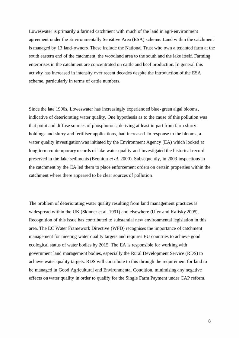
Cyanobacteria dominated the phytoplankton at all times of year apart from in August when
small green algae with crypotophytes and chrysophytes were dominant (Fig. 3.8 b). The
relatively small importance of diatoms in the spring (Fig. 3.7) contrasts with the situation in
many other English lakes. For example in lakes in the Windermere catchment, Asterionella
can reach 5 000 to 10 000 cell cm-3 in spring in contrast to the 229 cell cm-3 recorded in
Loweswater in 2005 (Fig. 3.8a). The relatively small importance of diatoms explains why the
silica concentration did not fall substantially in the spring (Fig. 3.5c): silica did not fall until
after the small diatom peak in July (Fig. 3.7) which largely comprised Tabellaria flocculosa
var asterionelloides (Fig. 3.8a) with contributions from the centric diatom Cyclotella
comensis. The cyanobacterium Planktothix mougeotii was probably the most abundant
phytoplankton species in Loweswater during the 12-month study. The population started to
increase in December 2004 and continued gradually up to a peak in April 2005 (Fig. 3.8c). At
other times taxa such as Woronichinia naegeliana, Aphanizomenon flos-aquae and Anabeana
flos-aquae contributed to the cyanobacterial population.
0
50
100
150
200
250
Aug-04 Oct-04 Dec-04 Feb-05 Apr-05 Jun-05 Aug-05 Oct-05
Cel
l den
sity
(cel
l cm
-3)
Asterionella formosaAulacoseira subarcticaTabellaria flocculosa var. asterionelloides
a)
0
2000
4000
6000
8000
10000
Aug-04 Oct-04 Dec-04 Feb-05 Apr-05 Jun-05 Aug-05 Oct-05
Cel
l den
sity
(cel
l cm
-3)
0
4000
8000
12000
16000
20000
Rhodomonas sp.Chrysochromulina parvaChlorella sp.
b)
0
5
10
15
20
25
30
35
Aug-04 Oct-04 Dec-04 Feb-05 Apr-05 Jun-05 Aug-05 Oct-05
Fila
men
t len
gth
(mm
cm
-3)
0
20
40
60
80
100
120
140
160
Col
ony
dens
ity (
colo
nies
cm
-3)
Woronichiniana naegelianaPlanktothrix mougeotii
c) Figure 3.8 Seasonal changes in representative phytoplankton. a) three diatoms; b) three small unicellular algae, note numbers of Chrysochromulina refer to the right-hand scale, peak cell density (cell cm-3) of 16 355 in July and for Chlorella 40 291 in August (N.B. peaks not shown); c) two cyanobacteria, Woronichinia colony density and Planktothrix filament length.

19
2.4 Discussion
Loweswater undergoes a thermal stratification pattern that is typical of relatively deep lakes in
this region and, during the summer, separates the warm upper layer (epilimnion) from the
cool lower layer (hypolimnion). Because Loweswater is relatively productive, substantial
oxygen depletion occurs at depth within the hypolimnion during the summer. This is likely to
allow the release of phosphate from the sediment into the hypolimnion (Mortimer, 1941,
1942) and this is potentially available to drive further algal production.
Phosphate is probably the main nutrient controlling phytoplankton production in Loweswater
(the ‘limiting’ nutrient) since the concentration of available phosphorus, i.e. SRP, is extremely
low throughout the growing season. In contrast, nitrate is only slightly depleted in late
summer. Silica, unusually, remained high during spring and did not become depleted until
mid-summer. This appears to have been because the spring bloom largely comprised
cyanobacteria, particularly Planktothrix mougeotii, which do not require silica, in contrast to
the normal pattern of a silica-requiring diatom spring bloom. The spring bloom in mid-May
produced the 12-month maximum chlorophyll a concentration of 27 mg m-3 : the
concentration in late summer was lower, at 18 mg m-3.
One of the features of Loweswater that appears to have a strong effect on its limnology is its
relatively long average retention time of about 199 days (Table 1.1). This compares with a
lake such as Grasmere that has exactly the same surface area but has an average retention time
of only 32 days. The long retention time in Loweswater relates, in part, to the relatively small
catchment area in relation to the lake volume but mainly to the relatively low rainfall in this
catchment compared to the other areas of the English Lake District (NERC, 2000). This is a
result of the geographical position of the Loweswater catchment on the western edge of the
north lakes adjacent to the Solway plain. The long retention time has a number of
implications. First, for a given nutrient load the amount of phytoplankton biomass that can be
supported is greater in a lake with a long retention time because the rate of algal loss through
hydraulic flushing is relatively low. The long retention time also allows relatively slow-

20
growing organisms, such as filamentous cyanobacteria, to develop whereas they may not be
able to do so in a more rapidly flushed lake. This may also explain the unusual spring bloom
dominated by cyanobacteria rather than diatoms. Later in the summer, the relatively low
hydraulic discharge will limit the amount of nutrients delivered to the lake from the
catchment. This will tend to reduce a summer phytoplankton bloom unless it can be supported
by recycling of nutrients within the lake.
The insights into how Loweswater functions that have been derived from this monthly study
will be used in the following sections that discuss long-term changes in the lake, sources of
nutrient loads to the lake and lake modelling to forecast the effect of different nutrient
reduction scenarios on water quality in the lake.

21
3. Changes in water quality in Loweswater using historic and contemporary data
3.1 Introduction
Based on an analysis of sediment cores from the lake, Bennion et al. (2000) found that the
nutrient status of Loweswater was stable from the 1300s to about 1850 when the first slight
evidence of nutrient enrichment was detected. This was followed by more profound nutrient
enrichment starting around 1950. Bennion et al. (2000) used contemporary evidence to
conclude that the nutrient status of the lake was current ly somewhere between mesotrophic
and eutrophic although they found that different measures (phytoplankton, macrophytes,
invertebrates etc) gave a range of trophic assessments. Part of the variation may have resulted
from the rate of response of different groups to changes in trophic status. However, the
categories themselves are imprecise and, as Bennion et al. (2000) acknowledged, it is difficult
to make comparisons across years where the frequencies and methods of data collection
differed.
This section of the report does not repeat the assessment and findings in the report of Bennion
et al. (2000). Instead, it uses a separate source of relatively recent information that was not
available to these authors, the so-called ‘Lakes Tour’ data collected by CEH and its
predecessors (FBA and IFE) since 1984. The Lakes Tours collect information on the 20 major
lakes and tarns in the English Lake District four times a year. Lakes Tours were carried out in
1984, 1991, 1995, 2000 and 2005. Since 1991, the data have been collected in a consistent
way. These data are analysed here to give a picture of recent changes in water quality. This
updates the preliminary analysis produced in April 2005, which was completed before all of
the most recent Lakes Tour data had been collected.
3.2 Materials & Methods
Information on the standardised procedures used in the Lakes Tour is given in Parker et al.
(2001). Note that in 1991 the mid-summer samples were collected in early August (8th) but
have been treated as if they were collected in July for ease of analysis and presentation.
22
3.3 Results
3.3.1 Alkalinity
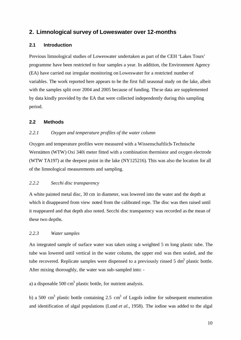
The mean alkalinity at Loweswater between 1974 and 1976 (29 samples) was 175 mequiv m-3
(Carrick & Sutcliffe, 1982). Alkalinity was essentially unchanged in 1984 and 1991 but since
then there has been a tendency for alkalinity to increase (Fig. 3.1). This increase in alkalinity
is statistically significant for January (Table 3.1). The tendency for an increase in alkalinity in
recent years could be caused by liming in the catchment (although this was carried out for the
first time for many years in 2005, K. Bell pers.comm) or reduced atmospheric deposition of
sulphur as ‘acid rain’, or both. Sulphate concentrations in Loweswater have fallen from an
annual average of 171 mequiv m-3 in 1975 through 116 mequiv m-3 in 2000 (Parker et al.,
2001) to 112 mequiv m-3 in 2005 (CEH unpublished data) as a result of a decline in the
sulphur component of acid rain. It could also result from increased use of nitrate (see Section
4.3.3) as this also generates alkalinity within the lake.
There has also been a tendency for pH to increase (Table 3.1) as would be expected if
alkalinity increased. There have been no long-term changes in the average concentration of
CO2 in the lake between 1984 and 2005 (data not shown).
0
50
100
150
200
250
300
350
1975 1980 1985 1990 1995 2000 2005
Alk
alin
ity (
meq
uiv
m-3
)
Jan
Apr
Jul
Oct
Figure 3.1. Alkalinity in Loweswater between 1975 and 2005 at four different times of year.

23
3.3.2 Total Phosphorus
Phosphorus (P) is the main nutrient that controls phytoplankton production in the larger lakes
of the English Lake District although nitrogen may be equally important in small upland tarns
(Maberly et al., 2002). To illustrate the importance of P, Figure 3.2 shows the average
phytoplankton as chlorophyll a plotted against the maximum concentration of total
phosphorus (TP) for the 20 lakes and tarns surveyed during the 2005 Lakes Tour. There is a
clear correlation (P<0.001) between chlorophyll a and TP concentrations. Furthermore,
Loweswater is also clearly P- limited since its position is close to the regression line which
represents the average relationship between chlorophyll a and TP for the 20 lakes and tarns.
Table 3.1. Correlation coefficient and probabilities of long-term change in limnological variables in Loweswater. Probability designated as * = P<0.05; ** = P<0.01, other correlations not significant. Not appropriate to test indicated by ‘n/a’.
Variable Range of
years January April July October Annual mean
Total P 1984-2005 0.11 0.91* 0.79 0.88 0.92*
SRP 1984-2005 0.30 -0.69 -0.69 0.33 0.22
NO3-N 1984-2005 -0.17 -0.71 -0.97** -0.91* -0.95**
SiO2 1984-2005 0.66 0.85 0.66 0.18 0.86
pH 1975-2005 0.73 0.63 0.70 0.55 n/a
Alkalinity 1975-2005 0.87* 0.58 0.37 0.72 0.71
Chl a 1991-2005 0.17 0.89 0.63 0.32 0.88
Secchi depth 1991-2005 -0.29 -0.85 -0.18 -0.84 -0.57
O2 at 12 m 1984-2005 n/a n/a -0.91* n/a n/a

24
y = 0.79x - 7.24R2 = 0.76
0
10
20
30
40
0 10 20 30 40 50 60
Maximum TP (mg m-3)
Ave
rage
Chl
a (
mg
m-3)
Figure 3.2. Average phytoplankton chlorophyll a as a function of annual maximum concentration of total phosphorus based on the 20 lakes forming the Lakes Tour in 2005. Loweswater is shown by the open symbol.
There has been a general trend of increasing total phosphorus concentration in Loweswater
since 1984 (Fig. 3.3). The annual mean concentration of TP has increased significantly over
this time period, as has the concentration in April (Table 3.1). The concentrations of TP in
2005 were very slightly lower than in 2000: annual mean of 15.4 compared to 16.5 mg m-3.
This difference is fairly small and probably not statistically significant given the seasonal
variation, but it is possible that the trend of increasing TP may have become slower or even
been reversed over time.

25
0
5
10
15
20
25
1975 1980 1985 1990 1995 2000 2005
Tota
l P (m
g m
-3)
Jan
Apr
Jul
Oct
Figure 3.3. Concentration of total phosphorus in Loweswater between 1984 and 2005 at four different times of year.
3.3.3 Soluble Reactive Phosphorus
Soluble reactive phosphorus (SRP) is the form of phosphorus that is readily available to
phytoplankton, and is more or less equivalent to phosphate. Although closely linked to
available phosphorus, the concentration of SRP can change rapidly in response to supply and
demand, so it is less reliable as an indicator of the trophic state of a lake than total
phosphorus. The concentration of SRP was very high in January 1995 and 2000 but
substantially lower in 2005 (Fig. 3.4). This may suggest a slight improvement in nutrient
concentrations but could equally result from chance and the precise timing of microbial
phosphorus-uptake prior to sampling. There have been no statistically-significant long-term
trends in SRP concentration(Table 3.1), possibly because this nutrient is very dynamic.

26
0
1
2
3
4
5
6
1975 1980 1985 1990 1995 2000 2005
Sol
ube
reac
tive
P (
mg
m-3
)Jan
Apr
Jul
Oct
Figure 3.4. Concentration of soluble reactive phosphorus in Loweswater between 1984 and 2005 at four different times of year.
3.3.4 Nitrate
Concentrations of NO3-N in January have been fairly constant, varying between 546 and 728
mg m-3. The low value in 1995 occurred in a winter with a highly positive North Atlantic
Oscillation Index (NAOI). The NAOI reflects the location of pressure systems in the North
Atlantic and controls winter weather in Western Europe. George et al. (2004) showed that for
lakes in the Windermere catchment a positive NAOI is correlated with mild winters and
relatively low concentrations of nitrate. The low winter value in 1995 may therefore result
from the positive NAOI. Although concentrations of winter nitrate in Loweswater show no
clear trend, there has, in contrast, been a strong tendency for concentrations of nitrate in July
and October to decline (Fig. 3.5). This reduction is highly significant (Table 3.1). The pattern
of relatively constant winter concentrations but declining summer concentrations suggests that
the summer decline is caused by processes within the lake. This is consistent with increasing
productivity caused by increasing availability of phosphorus which, in turn, increases the
demand for nitrogen.

27
0
200
400
600
800
1975 1980 1985 1990 1995 2000 2005
NO
3-N
(mg
m-3
)
Jan
Apr
Jul
Oct
Figure 3.5. Concentration of nitrate-nitrogen in Loweswater between 1984 and 2005 at four different times of year.
3.3.5 Silica
Silica is an important nutrient for several types of phytoplankton but is an essential
requirement for diatoms which use it to produce the outer cell-wall or frustule. There has been
a tendency for concentrations of silica (SiO 2) to have increased in Loweswater since 1984
(Fig. 3.6) although none of the trends are statistically significant (Table 3.1). The relatively
high concentrations of SiO 2 in April in 2000 and 2005 in comparison with 1984 and 1991
appears to result from a combination of relatively higher winter concentrations of SiO 2 and a
low level of SiO2 removal in the lake.

28
0
0.5
1
1.5
2
2.5
1975 1980 1985 1990 1995 2000 2005
SiO
2 (g
m-3
)Jan
Apr
Jul
Oct
Figure 3.6. Concentration of silica in Loweswater between 1984 and 2005 at four different times of year.
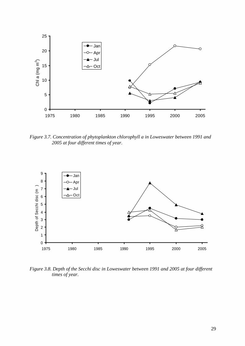
3.3.6 Phytoplankton chlorophyll a and Secchi depth
Since the first available data collected during the Lake Tour in 1991, there has been a large
increase in the concentration of phytoplankton chlorophyll a in April which was maintained
in 2005 (Fig. 3.7). All of the months, and the annual average, showed positive increases in
chlorophyll a concentration although none of the correlations against time were statistically
significant (Table 3.1). Since 1995, there has been a steady increase in chlorophyll a recorded
in January, July and October (Fig. 3.7). The Secchi depth showed an approximately inverse
pattern over the same period with tendencies for Secchi depth to decrease (i.e. for the lake
water transparency to decline) in April and October (Fig. 3.8), although the reduction is not
quite statistically significant (Table 3.1).
29
0
5
10
15
20
25
1975 1980 1985 1990 1995 2000 2005
Chl
a (
mg
m-3
)
Jan
Apr
Jul
Oct
Figure 3.7. Concentration of phytoplankton chlorophyll a in Loweswater between 1991 and 2005 at four different times of year.
0
1
2
3
4
5
6
7
8
9
1975 1980 1985 1990 1995 2000 2005
Dep
th o
f Sec
chi d
isc
(m)
Jan
Apr
Jul
Oct
Figure 3.8. Depth of the Secchi disc in Loweswater between 1991 and 2005 at four different times of year.

30
3.3.7 Oxygen concentration at depth
Oxygen depletion at depth during summer stratification is a symptom of eutrophication since
it occurs as a result of the decomposition of organic material produced in the upper layers of
the lake. Results from the ‘Lakes Tours’ dataset document a continued reduction in oxygen
concentration at depth during the summer. In 1984, the lowest oxygen concentration recorded
at depth was 3.3 g m-3. By 1991 and 1995, essentially zero (< 0.5 g m-3) oxygen
concentrations were recorded below a depth of 14 m (Fig. 3.9). This low oxygen
concentration was found at 12 m by 2000 and between 9.5 and 10 m in 2005. There has thus
been a progressive reduction in the depth at which oxygen depletion takes place. For example,
the reduction in oxygen concentration at 12 m depth has declined significantly between 1984
and 2005 (Table 3.1). This indicates an increase in the productivity and eutrophication of the
lake over the last 21 years.
0
2
4
6
8
10
12
0 2 4 6 8 10 12 14 16
Depth (m)
[O2 ]
(g m
-3)
19841991
19952000
2005
Figure 3.9. Profiles of oxygen concentration in Loweswater in July between 1984 and 2005.

31
3.4 Discussion and Conclusions
The long-term data provides clear and consistent evidence of a lake that has experienced
nutrient enrichment. The driver for the change is probably phosphorus enrichment since this
appears to be the limiting nutrient in Loweswater. Records show that total phosphorus has
increased over the last 20 years. Using paleolimnological data on diatoms, Bennion et al.
(2000) reconstructed an estimated total phosphorus concentration for the lake of about 10 mg
m-3, with a range of from 6 to 13 mg m-3, for the period before 1850. The morpho-edaphic
index approach of Chiaudani & Vighi (1984) allows concentrations of TP in lakes to be
estimated based on their alkalinity and mean depth. Using this approach with coefficients
developed specifically for UK lakes (Carvalho et al., 2004), a mean depth of 8.4 m and a
mean alkalinity of 184 mequiv m-3, the predicted concentration of TP for Loweswater is 8.6
mg m-3. This is similar to the estimate of Bennion et al. (2000). The paleolimnological
approach suggests that the concentration of TP increased after 1850 up to present day values
of about 15 to 20 mg m-3. These estimated concentrations broadly match contemporary
measurements.
These increases in phosphorus concentration will allow greater phytoplankton productivity.
Data from 1991 suggest an upward trend in phytoplankton chlorophyll a which, although not
quite statistically significant is fairly clear. This is particularly true for the spring bloom
which is driven by nutrients derived directly from the catchment rather than nutrients that are
recycled within the lake, which is probably important in the summer. The greater
phytoplankton productivity is linked to the lower water transparency, the greater depletion of
nitrate in the summer and the greater depletion of oxygen at depth. This latter fact will
probably facilitate release of phosphorus from the sediments to the water by reducing the
redox potential of the surface sediment (Mortimer, 1941, 1942) and so have a positive
feedback on eutrophication.
Lakes can be classified into different trophic states using various measures of lake
productivity. One widely used set of trophic states definitions is set out below in Table (3.2).
Note that although the category boundaries are relatively arbitrary, they can indicate changes
in the trophic category of a lake.

32
Table 3.2. Trophic categories based on different limnological characteristics following
OECD (1982)
In addition, the European Commission Water Framework Directive (WFD; 2000/60/EEC)
defines the ecological status of a lake in terms of a number of ecological criteria according to
the type of lake. In the typology used for UK lakes, Loweswater was categorised as a low
alkalinity lake (< 200 mequiv m-3) in 1984-2000 but crossed to a moderate alkalinity lake
(200 - 2000 mequiv m-3) in 2005. Loweswater with a mean depth of 8.4 m (Table 1.1) is
classified as a shallow lake using the UK typology (mean depth between 3 and 15 m). The
annual mean chlorophyll a concentrations for low and moderate alkalinity shallow lakes are
shown in Table 3.3. In the UK, site-specific reference mean concentrations of TP can be
estimated using the morpho-edaphic index approach of Chiaudani & Vighi (1984), as outlined
above. These reference and boundary values for the different ecological statuses for
Loweswater are shown in Table 3.3.
Trophic category Mean Total Phosphorus
(mg m-3)
Mean Chlorophyll a (mg m-3)
Maximum Chlorophyl a (mg m-3)
Mean Secchi depth (m)
Minimum Secchi depth
(m)
Ultra-oligotrophic < 4 < 1 <2.5 > 12 > 6
Oligotrophic 4-10 1-2.5 2.5-8 12-6 6-3
Mesotrophic 10-35 2.5-8 8-25 6-3 3-1.5
Eutrophic 35-100 8-25 25-75 3-1.5 1.5-0.7
Hypertrophic > 100 > 25 >75 < 1.5 < 0.7

33
Table 3.3. Current suggested Water Framework ecological status for Loweswater. Total phosphorus is a site-specific value calculated from the morpho-edaphic index using mean depth and the average alkalinity. Chlorophyll a is a type specific value. In each case the values refer to the annual mean.
Chlorophyll a (mg m-3) TP (mg m-3) Ecological status
1984-2000 2005 All years
High 3 4 8.6
High/Good 4 5 11.3
Good/Moderate 5 8 17.6
Moderate/Poor 10 16
The rather broad estimates of trophy and ecological status of Loweswater shown in Table 3.4
reflect the decline in the water quality that has already been described. In the last 20 years the
lake has changed from a mesotrophic lake to one that is on the mesotrophic-eutrophic
boundary. In terms of the Water Framework, the chlorophyll a concentration suggests that the
lakes is only at moderate ecological status. The annual mean concentration of TP (maximum
of 16.5 mg m-3 in 2000) is just above the moderate boundary (17.6 mg m-3) for this lake. One
reason for the slightly worse ecological status for the lake based on chlorophyll a rather than
TP is that Loweswater has a relatively long mean retention time (199 days, Table 1.1) for a
shallow lake giving more opportunity for biomass to accumulate.

34
Table 3.4. Assessment of trophic state and ecological status of Loweswater in different years for different variables. For trophic state: O = oligotrophic; M = Mesotrophic and E = eutrophic. For WFD: H = high; G = good; M = moderate and P = poor. Category boundaries for trophic state given in Table 3.2 and for WFD in Table 3.3.
Year Mean TP
Mean Chl a
Max Chl a
Mean Secchi
Min Secchi
WFD
TP
WFD Chl a
1984 M - - - - High -
1991 M M M M O Good Mod
1995 M M M M O Good Mod
2000 M E M E M Good Mod
2005 M E M E M Good Mod
The Water Framework Directive requires the water quality of Loweswater to be improved
from Moderate to Good ecological status by 2015. Table 3.3 suggests that Loweswater should
have a TP concentration of 8.6 mg m-3 based on its alkalinity and mean depth which is
broadly the concentration before 1850 (Bennion et al. 2000). The higher concentrations
recorded in recent years will be caused by additional sources of nutrients such as from human
waste, animal waste or fertilisers applied to the catchment to increase agricultural production.
The sources of the documented nutrient enrichment of the lake are investigated in the section
below. Reducing nutrient losses from these sources will be required in order to comply with
the Water Framework Directive.
The analysis of historical data gives some grounds for hope that the rate at which water
quality is declining has slowed down, and that there are some slight signs of improvement.
These may just be the result of year-to-year variation, but could also result from the changes
that have already been implemented in the catchment such as reducing the amount of
phosphorus applied in fertiliser to the fields. Further monitoring is required to distinguish
between these two possibilities- see final section.

35
4. Assessment of nutrient load to the lake
The load of phosphorus to a lake is a key factor in controlling its productivity. That load can
be estimated in a variety of ways. This section of the report uses three of the available
approaches to estimate the phosphorus load to Loweswater from its catchment. These are:
o Direct measurement
o Export coefficient modelling
o Calibrated nutrient runoff modelling
Since phosphorus is the main limiting nutrient in the lake (Sections 2 and 3), we will focus on
estimating loads of this nutrient although loads of nitrate and silica will also be estimated in
order to provide data for the PROTECH model in Section 5.
4.1 Nutrients loads from direct measurement
4.1.1 Introduction
The nutrient load to a lake cannot be measured directly, but it can be derived from two
components that can be measured. These are concentration (g m-3) and hydraulic discharge
(m3 time-1). The measured values are multiplied together to give the load, which has the units
of g time-1. Typically, ‘time’ is either a day or a year, depending on the purpose of the
estimate. It should be noted that small streams with high concentrations but low hydraulic
discharge may make a relatively low contribution to the total load to the lake, whereas large
streams with low concentrations but a high hydraulic discharges may make a relatively high
contribution.
In this section we report the estimated nutrient load from six streams that drain into
Loweswater, including the major inflow, Dub Beck. These loads are based on monthly
estimates of stream discharge and corresponding concentrations of TP, SRP, nitrate and silica.
Although accurate estimates of load can be achieved with frequent (i.e. daily) estimates of
concentration and discharge, those estimated from a less frequent sampling regime are less
reliable because the relationship between concentration and discharge is non- linear. The

36
propensity for sudden floods to transport a relatively large proportion of the load of a nutrient
(particularly those associated with particles, such as total phosphorus) over a very short
period, makes accurate estimates of load from infrequent measurements difficult to achieve.
This fact is reflected in the large range of equations that can be used to calculate load from
discharge and concentration (reviewed in Walling & Webb, 1985).
4.1.2 Methods
The stream sampling locations are given in Table 4.1. The site on Dub Beck upstream of the
Grange Hotel inflow was an additional site added in December 2004. At each stream site,
water temperature and conductivity were measured with a meter with inbuilt thermistor
(WTW Conduktometer LF1G1). Stream width was measured with a tape and stream depth
and flow were recorded at each of five positions across the stream. Flow was measured with a
propeller-type flow meter (Ott-Z30) at a third of the stream depth (representing the mean
velocity) and the number of revolutions of the propeller per minute was recorded: different
propeller types were used depending on the stream conditions and flow. The manufacturer’s
calibrations were used to convert revolutions per minute to flow (m s-1). Discharge (m3 s-1)
was calculated from stream width (m) and the average of the five products of stream depth
and flow (m2 s-1).
Table 4.1. Location of routine stream sampling sites in the Loweswater catchment.
Stream name Grid reference Subcatchment Area (ha)
Dub Beck upstream of Grange Hotel inflow NY115227 1 268
Dub Beck below Grange Hotel NY116225 1+2 297
Dub Beck (main inflow) NY118224 1+2+3 336
Miresyke Beck NY124222 4 5
Holme Beck NY122217 5 95
Beck below Hudson Place NY117222 6 8
At each site water was collected for analysis of pH, alkalinity, TP, SRP, nitrate and silicate.
An extra site was added on the beck that flows past the Grange Hotel and into Dub Beck (NY
114227), where only SRP was measured.

37
Figure 4.1. The Loweswater catchment showing the location of the routine stream sampling
sites. See Table 4.1 for grid references.
4.1.3 Results
The concentration results are presented first followed by estimates of load. In interpreting the
results is should be noted that high concentrations do not necessarily result in a high load. The
streams that drained catchments that were not intensively agricultural, i.e. Holme Beck and
Miresyke Beck, had alkalinities that were below 200 mequiv m-3 and at or below those of the
lake (Fig. 4.2). The sampling site on the main inflow, Dub Beck had an alkalinity that was
slightly higher than Loweswater (Fig. 4.2). The Beck draining Hudson Place had an extremely
high alkalinity suggesting that there was a large input of material, in addition to that derived
from the natural catchment, entering the lake from this beck. Apart from the Beck draining
Hudson Place, the pH in the streams was generally below that of Loweswater. This is a
typical pattern, because streams generally contain high concentrations of carbon-dioxide
derived from the soil water. This gas is lost in the lake, either into the atmosphere or in the
formation of organic matter in the form of phytoplankton.

38
0
0.2
0.4
0.6
0.8
1
1.2
Oct-04 Dec-04 Feb-05 Apr-05 Jun-05 Aug-05 Oct-05
Alk
alin
ity (e
quiv
m-3
)Dub Beck U/S of Grange Hotel Dub Beck below Grange Hotel
Dub Beck Main inflow Miresyke Beck
Holme Beck Beck below Hudson Place
Loweswater
a)
6
6.5
7
7.5
8
8.5
Oct-04 Dec-04 Feb-05 Apr-05 Jun-05 Aug-05 Oct-05
pH
Dub Beck U/S of Hotel GrangeDub Beck below Grange HotelDub Beck Main inflowMiresyke BeckHolme BeckBeck below Hudson PlaceLoweswater
b)
Figure 4.2. Seasonal changes in the monitored streams of concentrations of: a) alkalinity, and
b) pH. Values for Loweswater are shown for comparison.
39
0
40
80
120
160
200
Oct-04 Dec-04 Feb-05 Apr-05 Jun-05 Aug-05 Oct-05
Con
cent
ratio
n of
TP
(m
g m
-3)
Dub Beck U/S ofGrange HotelDub Beck belowGrange HotelDub Beck Main inflow
Miresyke Beck
Holme Beck
Beck Below HudsonBeckLoweswater
a)
0
20
40
60
80
100
120
Oct-04 Dec-04 Feb-05 Apr-05 Jun-05 Aug-05 Oct-05
Con
cent
ratio
n of
SR
P (
mg
m-3
)
Dub Beck U/S of Grange HotelDub Beck below Grange HotelDub Beck Main inflowMiresyke BeckHolme BeckBeck Below Hudson BeckHotelLoweswater
b)
0
5
10
15
20
25
30
Oct-04 Dec-04 Feb-05 Apr-05 Jun-05 Aug-05 Oct-05
Con
cent
ratio
n of
SR
P (
mg
m-3
)
Dub Beck U/S of Grange HotelDub Beck below Grange HotelDub Beck Main inflowMiresyke BeckHolme BeckBeck Below Hudson BeckHotelLoweswater
c)
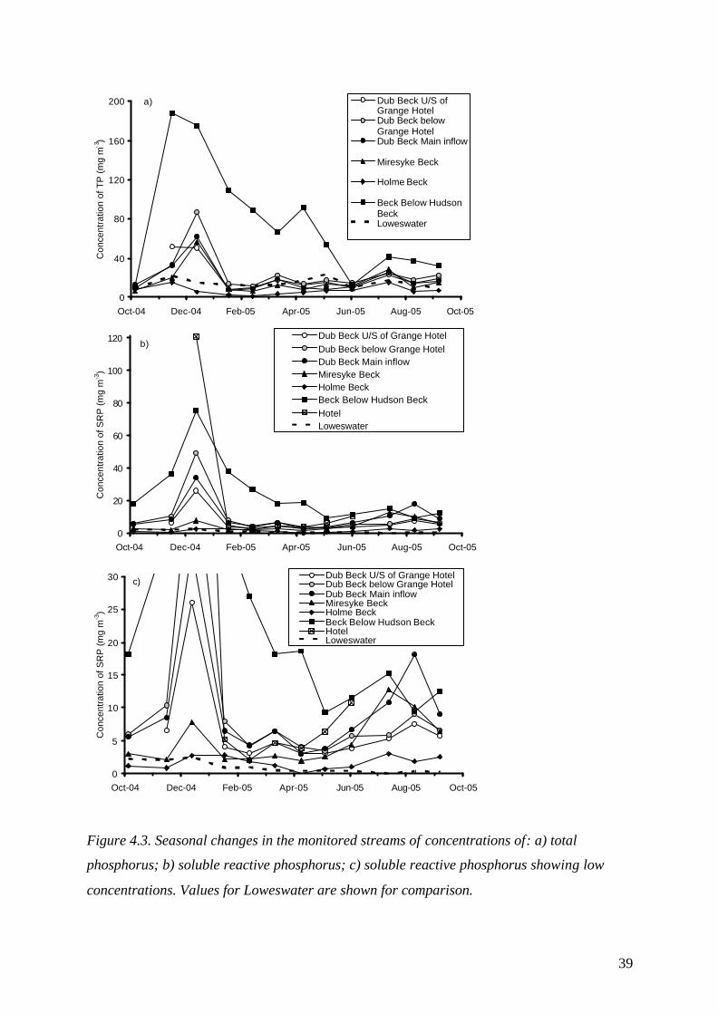
Figure 4.3. Seasonal changes in the monitored streams of concentrations of: a) total
phosphorus; b) soluble reactive phosphorus; c) soluble reactive phosphorus showing low
concentrations. Values for Loweswater are shown for comparison.
40
Holme Beck, which drains woodland on the western shore of Loweswater has a lower
concentration of total phosphorus (TP) than the lake (Fig. 4.3a). The other streams tend to
have a higher concentration of TP, particularly the stream draining Hudson’s Place. This had
very high concentrations in November and December 2004 that declined slightly later in
2005. The main inflow, Dub Beck, also had elevated concentrations of TP, particularly in
December 2004. The concentrations upstream of the hotel were similar to that close to the
inflow to the lake which suggests that the catchment above the hotel is the major source of the
high TP although the Hotel does seem to be contributing some TP (see below).
The pattern of concentrations of soluble reactive phosphorus (SRP) is similar to that for TP
(Fig. 4.3). Concentrations were generally highest in the beck draining Hudson’s Place, apart
from one very high concentration in mid December 2004 in the beck passing past the Grange
Hotel. This beck clearly contributes to the concentration of SRP as the concentration is higher
immediately downstream of its confluence with the main inflow (Fig. 4.3b,c).
Mapping the average concentrations of TP in the inflowing streams shows the very high
concentrations in the beck draining Hudson’s Place and the high concentrations in the main
inflow, Dub Beck (Fig. 4.4).

41
Figure 4.4. Spatial variation in mean TP concentrations at the routine sampling sites. Numbers in boxes refer to subcatchments.
0
1000
2000
3000
4000
5000
6000
Oct-04 Dec-04 Feb-05 Apr-05 Jun-05 Aug-05 Oct-05
Con
cent
ratio
n of
NO
3-N
(mg
m-3
)
Dub Beck U/S ofGrange HotelDub Beck belowGrange HotelDub Beck Main inflow
Miresyke Beck
Holme Beck
Beck Below HudsonBeckLoweswater
a)
0
1
2
3
4
Oct-04 Dec-04 Feb-05 Apr-05 Jun-05 Aug-05 Oct-05
Con
cent
ratio
n of
SiO
2 (m
g m
-3)
Dub Beck U/S of Grange Hotel Dub Beck below Grange HotelDub Beck Main inflow Miresyke BeckHolme Beck Beck Below Hudson Beck
Loweswater
b)
Figure 4.5. Seasonal changes in the monitored streams of: a) nitrate; b) silica. Values for
Loweswater are shown for comparison.
The seasonal pattern for changes in concentration of nitrate (Fig. 4.5a) is similar to that for
TP. The concentration in Holme Beck is lower than that in the lake, but the concentration in
the other inflowing streams is higher. The main inflow, Dub Beck, had substantially higher
concentrations of nitrate than the lake. The nitrate concentration in the beck draining
Hudson’s Place was very high in January, February and March 2005 but on other sampling

42
occasions was very similar to Dub Beck. Silica concentrations were generally higher in all of
the streams than the lake. The concentration in the lake was similar to that of Dub Beck apart
from when the concentration in the lake fell during summer 2005 as a results of a modest
growth of diatoms (Fig. 4.5b). Concentrations of silica in the beck draining Hudson’s Place
was similar to that in the other inflowing streams.
The average concentrations for the monitored subcatchments are shown in Table 4.2. These
data highlight the low nutrient concentrations of nitrogen and phosphorus in subcatchment 5
(Holme Beck) compared to subcatchment 6 (Beck draining Hudson’s Place).
Table 4.2 Mean concentration (mg m-3) of nutrients in the monitored streams over twelve months.
Subcatchment Total P SRP NO3-N SiO2
1 21.5 6.6 1445 2291
1+2 24.4 9.9 1540 2283
1+2+3 19.3 9.7 1590 2335
4 16.7 4.8 1014 2835
5 6.8 1.7 176 2749
6 75.8 24.1 1979 2905
As mentioned above, load can be derived from the product of measured concentration and
hydraulic discharge. The average daily load for the streams monitored in the 12-month study
is shown in Table 4.3.

43
Table 4.3 Estimated mean discharge (m3 s-1) and average load (mg s-1) for nutrients in the
monitored streams over twelve months. *Total is based on catchments 1, 2, 4, 5 and 6,
see text.
Subcatchment Discharge Total P SRP NO3-N SiO2
1 0.341 12.46 6.26 433 522
1+2 0.395 27.9 15.4 621 725
1+2+3 0.251 10.6 5.5 412 491
4 0.007 0.094 0.020 8.2 0.2
5 0.047 0.33 0.07 9.4 1.3
6 0.004 0.40 0.16 6.9 0.1
Total* 0.453 28.7 15.7 646 727
Table 4.3 shows that the stream location on the main inflow to Dub Beck (draining
subcatchments 1+2+3) may have some problems in relation to the measurement of discharge
since the average discharge there is lower than at the two points immediately above it (i.e.
draining subcatchments 1 and 2). Alternatively, it is possible that there is some loss of water
from the stream into the groundwater or into the surrounding bog between the monitoring site
on Dub Beck below the Grange Hotel and that near the lake. Whatever the reason, when
calculating loads we have used the input from subcatchments 1 + 2, rather than the input from
1 + 2 + 3, as our estimate of load from Dub Beck.
The table of loads (Table 4.3) shows that the high P concentrations at the Beck below
Hudson’s Place in subcatchment 6 do not translate into a large load to the lake because the
hydraulic discharge is relatively low. The main load comes from the main inflow, Dub Beck,
which contributes about 97% of TP, 98% of SRP, 96% of NO3-N and 99% of the total
monitored load of SiO 2.
The loads estimated here are necessarily rough approximations because they are based on
monthly samples. Ideally daily samples are needed to provide a more detailed estimate of load
because load can be highly discontinuous and the load of many chemicals, particularly those
associated with particulate material, is often produced by relatively few high-flow events.

44
This is illustrated by the storm on 14 December 2004, which happened to coincide with one
of our routine sampling events. Table 4 shows that a large percentage of the estimated total
load of TP was delivered in that storm. On that day, the measured flow in the Dub Beck was
2.8 m3 s-1. Data from the Environment Agency flow records suggest that high flow events,
greater than 2 m3 s-1, may occur five to six times a year in winter: the extra load of nutrients
that these storm events contribute to Loweswater have not been measured in this study and so
our estimate of load is likely to be an underestimate. The effect of the 14 December storm on
delivering extra load to the lake appeared to be particularly marked on Dub Beck just
downstream from the confluence with the beck flowing past the Grange Hotel. Measurements
on this ‘Hotel Beck’ confirmed that it carried a high concentration of TP and SRP at this time.
This suggests that there is a localised source of pollution in this subcatchment that is related to
high flow events, such as septic tank or slurry pit overflow or washoff from paved areas
associated with animal husbandry.
Table 4.4. Contribution of the storm event on 14 December 2004 to total annual TP load.
Measured TP load (kg P y-1) Subcatchment Excluding
storm Storm
event only Total
Storm event as % of total
1 62.5 6.3 68.8 10.0 1 + 2 57.2 14.1 71.3 24.7 1 + 2 + 3 67.4 5.0 72.4 7.4 4 2.5 0 2.5 0 5 12.0 0 12.1 0 6 (part) 5.8 0.1 5.9 1.7 Total (1 + 2 + 3 + 4 + 5 + 6)
87.7 5.1 92.9 5.8
This study has given a general idea of the magnitude of the loads entering the lake and
suggested areas that may be the major sources of phosphorus. However, direct measurement
of nutrient loads to a lake is difficult to achieve with a high degree of certainty. One drawback
is that not all streams can be monitored. This is partly covered in the next section (4.2) where
all possible streams were monitored on one occasion. The second problem with direct
measurements is that the temporal resolution is rarely sufficient to account for all inputs,
particularly those associated with storm events. These temporal and spatial problems are
addressed using a completely different approach, export coefficient modelling, in Section 4.4.

45
4.2 Survey of streams for high concentrations of phosphate
4.2.1 Introduction
The seasonal study measured concentrations and estimated loads of phosphate from six
streams every month for 12 months. These streams were chosen using local knowledge of
natural and possible phosphorus-enriched streams. Time and money did not allow every
possible stream to be sampled in this way, but to obtain a broader view of other possible
phosphorus sources to the lake as many streams as possible were sampled on one occasion.
4.2.2 Methods
On 5/11/2005, a day of very heavy rainfall, 24 inflow streams were sampled in the catchment.
At each stream encountered during a circumnavigation of the lake, position was located with
a GPS, temperature and conductivity was measured with a WTW Conduktometer LF1G1 and
a water sample was collected that was analysed for soluble reactive phosphorus (SRP) later
that day using the method given in Section 2.
4.2.3 Results & Discussion
The survey was undertaken during a period of heavy rain and so many streams were present,
including ones that would have been dry for much of the year. The survey confirmed the high
concentrations of SRP in the stream draining past Hudson’s Place (Stream 6) with a
concentration of 29 mg m-3. The survey also identified two other streams, not included in the
main survey, with high concentrations of SRP. One was at Stream 11, (Fig. 4.6; NY118219)
with a concentration of 17 mg m-3, the other drained from the area around Askhill (Stream 20;
NY118225) and had a concentration of 26 mg m-3. The results also confirmed that Crabtree
Beck (Stream 24), which has a sub-catchment of about 15% of the total and enters the lake
near the south-west end of the lake, had a very low SRP concentration of about 0.5 mg m-3,
and so is not a high-concentration source of phosphorus to Loweswater (Fig. 4.6).

46
Figure 4.6. Data from the survey of SRP concentrations in the Loweswater feeder streams, 5 November 2005. Numbers refer to stream sampling number.
There was a weak correlation between phosphate concentration and conductivity (Fig. 4.7),
with the three high SRP concentration streams having higher concentrations than expected
from the conductivity. This is perhaps evidence that the phosphate does not derive from
natural catchment-processes, but also means that conductivity cannot be used as a simple way
of checking for high inputs of SRP.

47
Figure 4.7. Relationship between concentration of soluble reactive phosphorus (SRP) and conductivity in the 24 streams flowing into Loweswater on 5/11/2005. The line of best fit and corresponding equation are shown.
4.3 Release of nutrients to streams as a result of farm management events
4.3.1 Introduction
The effect of specific management activities, such as muck-spreading and the application of
fertiliser, on the nutrient load to Loweswater were assessed by making daily measurements of
nutrient concentration in a stream adjacent to those management activities. This high
resolution sampling was possible by involving one of the farmers, Danny Leck, in the
sampling process.
4.3.2 Methods
Three management practices were monitored: a slurry application at the end of January 2005,
an application of fertilisers and slurry in March/ April and an application of fertilisers and
slurry in May. In all cases water samples were collected from Dub Beck on the main inflow
y = 0.17x - 8.96
R2 = 0.49
0
10
20
30
0 50 100 150 200 250
Conductivity (µS cm-1)
PO
4 -P
(m
g m
-3)

48
site below the field. Water was collected in bottles and stored in a refrigerator prior to
analysis for TP and nitrate using the methods described in Section 2.
4.3.3 Results
There was a strong, statistically significant, effect of rainfall (and hence discharge) on the
concentration of TP (Fig. 4.8). A linear regression produced a highly significant result (TP
concentration, mg m-3 = 8 + 2.1 * rainfall, mm d-1; r = 0.66, P<0.001). In contrast nitrate
concentration tended to decline with rainfall, possibly as a result of dilution (nitrate-N
concentration, mg m-3 = 1587 + 70.3 * rainfall, mm d-1, r = 0.45, P<0.05).
0
500
1000
1500
2000
2500
3000
Jan-05 Feb-05 Mar-05 Apr-05 May-05 Jun-05
NO
3-N
(m
g m
-3)
0
10
20
30
40
50
60
70
TP
(mg
m-3
) and
rain
fall
(mm
day
-1)
Nitrate Rainfall
TP
Slurry application
Fertilizer and slurry application
Fertilizer and slurry application
Figure 4.8. Effect of management practices on stream nutrients concentrations. Crosses show
the timing of the named management activities. Daily rainfall was provided by the
Environment Agency from their site at Cornhow.
The results also suggest a possible direct effect of management in adjacent fields on the
concentration of total phosphorus in the stream (Fig 4.8), but rainfall is needed to transport
the nutrient into the stream.

49
4.3.4 Discussion
The frequent measurements showed the importance of rainfall and discharge in influencing
the concentration of TP and nitrate. The decline in nitrate concentration with rainfall may
result from a dilution effect, while the increase in TP may result from increased input of
particulate material into the stream. The study was not able to prove definitively that
management activities had a direct effect on stream chemistry, although this is likely, because
we cannot exclude the effects of nutrient inputs upstream from the sampling site.
4.4 Total phosphorus load derived from export coefficients
4.4.1 Introduction
The annual TP load to a lake from its catchment can be estimated using an export (loss)
coefficient approach. This can be applied to both diffuse and point sources within the
catchment. For diffuse sources, this involves estimating the total area (Ai, hectares) of each
landcover type (i, 1 to n) within the catchment and multiplying these values by a
corresponding TP export coefficient (Ei, kg ha-1y-1), as obtained from the literature. The
resultant annual TP loss values for each landcover type are then summed to give the predicted
total annual TP load to the lake from runoff over the whole catchment (Prunoff , kg y-1), as
follows:
P A Erunoff i ii
n
= ×=
∑ ( )1
For sewage-related point sources, i.e. septic tanks in the case of the Loweswater catchment,
the size of the contribution (Pseptic, kg y-1) can be estimated on a per capita basis, as follows:
P N Eseptic septic= ×
50
where N is the estimated number of people in the catchment and Eseptic is the per capita TP
export coefficient for septic tanks. The total external TP load to the lake (Pload, kg y-1) can
then be calculated as the sum of the above, i.e.
septicrunoffload PPP +=
Other sources of TP can also be added to this calculation where sufficient data are available,
e.g. TP input to the lake from roosting birds, direct rainfall, etc. However, these inputs were
not included in the calculations for Loweswater because they were assumed to be very small
by comparison with the export of TP from land use and sewage related sources.
4.4.2 Methods
For this part of the study, the Loweswater catchment was subdivided into sub-catchments
corresponding to the upstream areas draining to the routine monitoring stations. A digital
outline of each sub-catchment was defined using a 50 m resolution digital terrain model
(DTM). The sub-catchment outlines (Fig. 4.9) were used to subdivide the catchment into
areas whose predicted total phosphorus (TP) loss, based on land cover information and known
sources of sewage effluent, could be compared to the measured values for validation
purposes. It was not possible to define the subcatchment draining to the Hudson Place Beck
sampling site in this way, because it was too small and there was too little variation in
topography in this area. So, the area of this subcatchment was calculated from the relationship
between the average discharge measured at the site and that measured at the Holme Beck
sampling site. The average discharge at Hudson Place Beck was only 8% of that measured at
Holme Beck, so the subcatchment area that drains to Hudson Place Beck was assumed to be
8% of that draining to the Holme Beck site, i.e. about 8 ha.
The TP export coefficients used for the Loweswater catchment are summarised in Table 4.5.
The landcover classifications in the Loweswater catchment, based on the LCM2000 landcover
map, are shown in Figure 4.10. The LCM2000 data incorrectly records arable land in several
areas, such as in the north-west corner of the catchment. When compared to recent aerial
photography, it can be seen that these areas are, in fact, areas of improved grassland. So, the
arable areas were reclassified as improved grassland for the purposes of this study.

51
Figure 4.9. Map of the Loweswater catchment showing the routine sampling sites and the subcatchments (1-5) that drain to them; subcatchment 6 was not sampled or gauged routinely.
Figure 4.10. Map of the Loweswater catchment showing land-cover within each of the sub-catchments (1-5) that were routinely sampled and sub-catchment 6.

52
Table 4.5. TP export coefficients for land cover types in the Loweswater catchment.
Landcover type TP export coefficient (kg ha-1 y-1)
Reference
Broadleaved woodland 0.15 Dillon & Kirchner (1975)
Coniferous woodland 0.15 May, Place, George & McEvoy (1996)
Improved grassland 0.38 May, Place, George & McEvoy (1996)
Rough grassland 0.07 Cooke & Williams (1973)
Bracken 0.10 Harper & Stewart (1987)
Bog 1.00 Casey, O'Connor & Green (1981)
Inland rock 0.10 May, Place & George (1995)
Urban/suburban development (runoff only)
0.83 Bailey-Watts, Sargent, Kirika & Smith (1987)
In addition to the losses from the land, the TP losses from other known sources must also be
included. In this case, these comprise effluent from domestic septic tanks associated with
permanent residences and holiday accommodation around the catchment, and that related to
cattle rearing.
As there are no sewage treatment works in this area, all residential accommodation is served
by septic tanks. The number of people served by septic tanks within each sub-catchment was
determined using data provided on the location of each property (Fig. 4.11) and the
corresponding annual occupancy, expressed as average number of ‘bed nights’ per year
(Leck, pers. comm.). The annual TP loss from these systems was calculated from these values
by multiplying the average occupancy of each property by a per capita TP export coefficient
associated with septic tanks effluent, i.e. 0.3 kg TP capita-1 y-1 (Carvalho et al., 2005). In
order to produce a worst possible case scenario for phosphorus loads from these systems,
TP losses were also calculated assuming no retention of phosphorus, i.e. that the septic tanks
were not working at all. The TP export coefficient for this scenario was estimated to be
1.2 kg TP capita-1 y-1, i.e. the per capita TP load to a septic tank (Carvalho et al., 2005).

53
Figure 4.11. Septic tanks and slurry pits within the Loweswater catchment, showing the
subcatchment draining to the Dub Beck (main inflow) sampling site.
The potential TP loss from the spreading of slurry and manure within the catchment was
estimated from information supplied by the farmers. This provided details of the number of
cattle being kept on each farm, the type of animal waste produced and the proportion of that
animal waste that is spread within the catchment. The average TP export coefficient from
cattle waste to water was estimated to be 0.14 kg capita-1 y-1, with an average of 373 cows
contributing to the slurry and manure that is spread within the catchment. Waste from the 280
remaining cattle is spread outside the catchment.
4.4.3 Results
The estimated TP load from each sub-catchment and the corresponding values obtained from
the routine water quality monitoring programme are shown in Table 4.6. Because the export
coefficient approach deals with average annual values from the literature and the measured
values are based on catchment specific monthly values, these values are not expected to agree
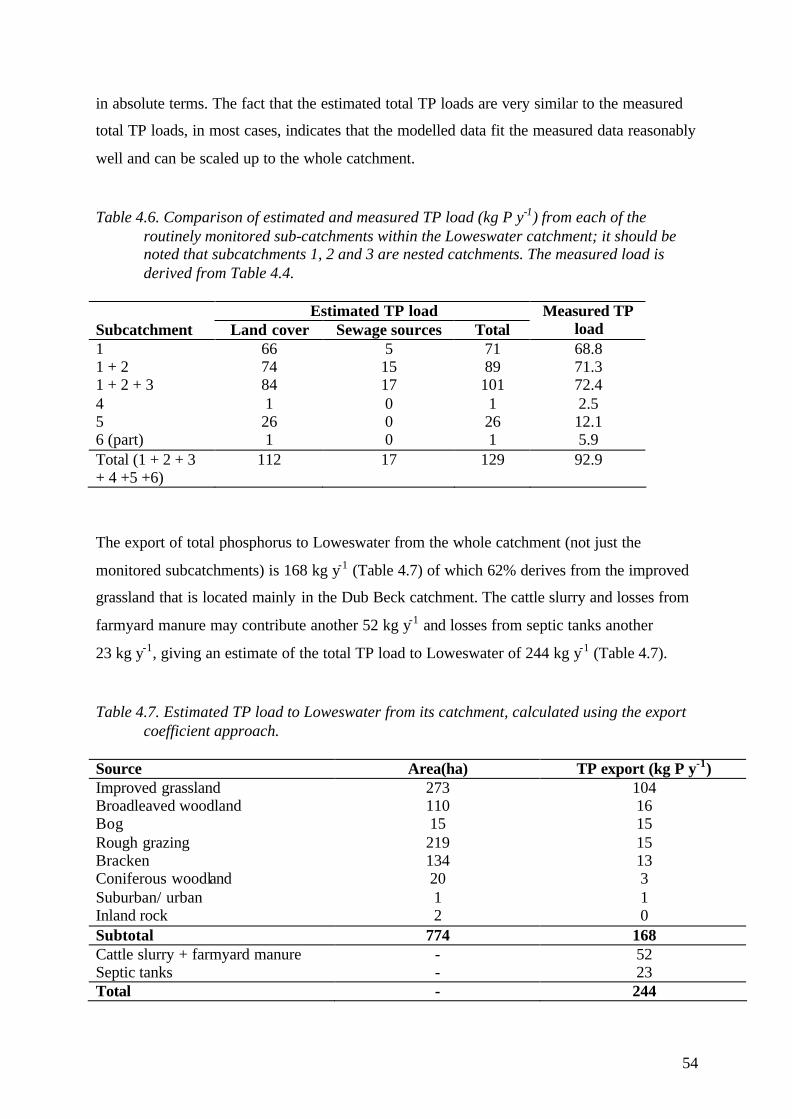
54
in absolute terms. The fact that the estimated total TP loads are very similar to the measured
total TP loads, in most cases, indicates that the modelled data fit the measured data reasonably
well and can be scaled up to the whole catchment.
Table 4.6. Comparison of estimated and measured TP load (kg P y-1) from each of the routinely monitored sub-catchments within the Loweswater catchment; it should be noted that subcatchments 1, 2 and 3 are nested catchments. The measured load is derived from Table 4.4.
Estimated TP load Subcatchment Land cover Sewage sources Total
Measured TP load
1 66 5 71 68.8 1 + 2 74 15 89 71.3 1 + 2 + 3 84 17 101 72.4 4 1 0 1 2.5 5 26 0 26 12.1 6 (part) 1 0 1 5.9 Total (1 + 2 + 3 + 4 +5 +6)
112 17 129 92.9
The export of total phosphorus to Loweswater from the whole catchment (not just the
monitored subcatchments) is 168 kg y-1 (Table 4.7) of which 62% derives from the improved
grassland that is located mainly in the Dub Beck catchment. The cattle slurry and losses from
farmyard manure may contribute another 52 kg y-1 and losses from septic tanks another
23 kg y-1, giving an estimate of the total TP load to Loweswater of 244 kg y-1 (Table 4.7).
Table 4.7. Estimated TP load to Loweswater from its catchment, calculated using the export coefficient approach.
Source Area(ha) TP export (kg P y-1) Improved grassland 273 104 Broadleaved woodland 110 16 Bog 15 15 Rough grazing 219 15 Bracken 134 13 Coniferous woodland 20 3 Suburban/ urban 1 1 Inland rock 2 0 Subtotal 774 168 Cattle slurry + farmyard manure - 52 Septic tanks - 23 Total - 244

55
Given the uncertainty in the total load of TP to Loweswater and to provide a range of possible
loads, six scenarios were produced illustrating a range of possible loads. These are shown in
Table 4.8. The calculations suggest that between 53% and 88% of the TP load derives from
the landcover.
Table 4.8. Scenarios of load of TP (kg y-1) to Loweswater.
Scenario Scenario description Individual load without landcover
Total load (% of load derived
from landcover) A Landcover only - 168 (100) B Landcover plus slurry and farmyard
manure (FYM) 52 220 (76)
C Landcover plus functioning septic tanks
23 191 (88)
D Landcover plus non-functional septic tanks
96 264 (64)
E Landcover plus slurry and FYM plus functioning septic tanks
75 243 (69)
F Landcover plus slurry and FYM plus non-functioning septic tanks
148 316 (53)
4.5 Loads of SRP based on a calibrated nutrient runoff model
4.5.1 Introduction
To assess the impact of the phosphorus load on the lake, it is necessary to generate daily input
data for the lake model, PROTECH (see Section 5), from the monthly measurements of
discharge and SRP concentrations. This was achieved using a calibrated nutrient runoff model
known as the Generalized Watershed Loading Functions (GWLF) model. GWLF is a non-
point source loading model in which the loading functions provide a practical compromise
between simple empirical export coefficient models that predicts annual values (e.g.
Section 4.4), and complex chemical simulation models that unrealistically large amounts of
data for most practical applications at the catchment scale. GWLF was originally developed
by Haith and Tubbs (1981) and validated by Haith and Shoemaker (1987) to simulate monthly
dissolved and total phosphorus and nitrogen loads in streamflow. There are several versions
of the original GWLF model currently in use. The version used in this project was created by

56
the New York City Department of Environmental Protection (NYCDEP) and runs within the
Vensim® visual modelling software package (Ventana Systems, Inc.). We are grateful to the
NYCDEP for allowing us to run their version of GWLF on the Loweswater catchment.
The GWLF model comprises two main components, a hydrological sub-model and a nutrient
delivery sub-model. It is driven by daily temperature and precipitation data for the catchment.
Water balances are calculated on a daily time step and, from this, streamflow is predicted
from runoff and sub-surface flow (Figure 4.12). The model then uses these hydrological
values to estimate nutrient delivery from land use, septic tanks and any other quantifiable
sources within the catchment. Nutrient runoff from diffuse sources is calculated as a function
of land use, with loads of dissolved nutrient being derived by multiplying hydraulic runoff by
land use specific nutrient concentrations. The model also estimates the contribution of
nutrients from septic tanks on the basis of values provided by the user detailing the number of
people being served by such systems at different times of year.
Figure 4.12. Diagrammatic representation of the hydrological part of the GWLF model.

57
4.5.2 Methods
For application to the Loweswater catchment, the hydrological part of the model was
calibrated using daily rainfall data from a rain gauge at the Cornhow sewage treatment works
(NY150222), and minimum and maximum air temperatures from a meteorological station at
Keswick, as input. Daily outflow monitoring data, provided by the Environment Agency
(EA), were used to validate the model output. Calibration was carried out for the period of
available data, i.e. 13 July 1999 to 30 June 2001. Figure 4.13 shows the calibrated model
output in comparison with the measured values. In general, the modelled values show a high
goodness of fit to the measured data (r2=0.8).
The nutrient delivery part of the GWLF model was calibrated using data obtained from the
‘Dub Beck (main inflow)’ sampling site (Figure 4.1) during this project, and information on
nutrient sources in the subcatchment upstream of this point. The latter included areal
landcover (Figure 4.10, Table 4.7) and the number and location of septic tanks (Figure 4.11).
0
0.5
1
1.5
2
2.5
3
Sep Dec Mar Jun Sep Dec Mar Jun
1999-2001
Str
eam
flow
(cm
)
Modelled values
Measured values
Figure 4.13. Comparison of modelled and measured streamflow for the Loweswater catchment after calibration; streamflow is expressed in centimetres, i.e. daily flow volume divided by catchment area.

58
Initial landcover-specific nutrient concentrations for the model (Table 4.5) were derived from
the corresponding phosphorus export coefficients for the Bassenthwaite catchment used by
May et al. (1994) (Table 4.2). The original values, expressed in kg P loss ha-1 y-1, were
converted to phosphorus concentrations (mg m-3) by dividing them by the average annual
hydraulic runoff over the catchment, estimated to be 14,750 m3 ha-1 y-1.
Septic tanks within the subcatchment were added to the model in terms of their estimated
person equivalent (PE) values. These amounted to 50 PE. For modelling purposes, it was
assumed that all of the septic tanks were functioning correctly and a per capita export
coefficient of 0.3 kg TP y-1 (Carvalho et al., 2005) was applied.
Table 4.9. Areal coverage and initial phosphorus concentration values for each land cover type in the catchment upstream of the ‘Dub Beck (main inflow)’ sampling site.
Land cover type Area (ha) TP concentration
(mg m-3)
Improved pasture 144.13 0.026
Broad leaved forest 15.16 0.010
Rough grazing 99.44 0.005
Urban/suburban runoff
1.38 0.056
Arable 41.80 0.017
Upland moor 30.49 0.007
Coniferous forest 2.31 0.010
The results of the nutrient delivery calibration on the Dub Beck subcatchment are shown in
Figure 4.13. The modelled data fitted the measured data reasonably well, except during the
storm event of 14 December 2004 when a very high SRP load was recorded. It was not
possible to generate this high value from the model, because the measured rainfall data (and,
consequently, the modelled streamflow) did not adequately reflect the heavy rainfall in the
upper catchment on that day. This was probably because the rain gauge, which is situated just

59
outside the southern end of the catchment, did not record this very local storm event in the
northern part of the catchment. The measured stream discharge rates across the catchment
appear to support this explanation. Discharge rates recorded in streams at the southern end of
the catchment on that day were similar to those recorded for those sites during the rest of the
year. However, the corresponding discharge rates in the northern part of the catchment on that
occasion were 30-40 times higher than those recorded during the rest of the year.
0
0.5
1
1.5
2
2.5
3
3.5
4
4.5
5
Sep-04 Nov-04 Jan-05 Mar-05 May-05 Jul-05 Sep-05
SR
P L
oad
(kg
d-1
)
Modelled valuesMeasured values
Figure 4.13. Comparison of modelled and measured values for SRP load after calibration of the GWLF model to the sub-catchment upstream of the ‘Dub Beck (main inflow)’ sampling site.
After calibration, the model was applied to the whole Loweswater catchment to generate daily
discharge rates and nutrient concentrations for input to PROTECH. Summary landcover data,
septic tank PEs (in this case, 80), daily rainfall data for Cornhow, and daily minimum and
maximum air temperature for Keswick were used as input to the model. In addition, the
minimum and maximum annual TP losses from septic tanks (see Section 4.4.2) and the
spreading of cattle waste within the catchment (see Section 4.4.2) were apportioned equally

60
across the 365 days of the year for input to the model under a range of phosphorus loading
scenarios.
The six scenarios of nutrient loading used in Section 4.4 and detailed in Table 4.8 were used
in the GWLF model.
4.5.3 Results
The daily output data were provided as input to the lake model, PROTECH, and are presented
here only as annual summaries to allow comparison of estimated annual SRP loads for the
different scenarios tested (Table 4.10). Note that the input of phosphorus from septic tanks
and animal husbandry is assumed to be as SRP so the figures for individual load in Table 4.10
are the same as in Table 4.8. The data suggest that the annual SRP load to the lake from its
catchment, assuming that all septic tanks are functioning correctly, would be 62 kg y-1. This
value is 32% of the annual TP load as calculated for this case using the export coefficient
approach (Section 4.4.3), a value that is only slightly lower than the average measured
percentage of SRP to TP for the catchment (35%). Under the ‘plus slurry and FYM plus
functioning septic tanks’ scenario, the corresponding value was 46%..
Table 4.10. GWLF output for the Loweswater catchment showing variation in predicted SRP loads (kg y-1) to the lake under various TP export scenarios. The SRP load as a percent of the TP load estimated from export coefficient modelling (Table 4.8) is also shown.
Scenario Scenario description Individual load without landcover
Total load (SRP as % TP load)
A Landcover only - 37 B Landcover plus slurry and farmyard
manure (FYM) 52 89 (41)
C Landcover plus functioning septic tanks
24 62 (32)
D Landcover plus non-functional septic tanks
96 132 (50)
E Landcover plus slurry and FYM plus functioning septic tanks
76 113 (47)
F Landcover plus slurry and FYM plus non-functioning septic tanks
148 183 (58)

61
4.6 Discussion
GWLF provides a fairly simple method of interpolating between infrequently measured data
values to provide daily input data for PROTECH. However, it relies heavily on reliable daily
rainfall values because both the hydrological and nutrient delivery parts of the model are
heavily dependent upon these. Within the Loweswater catchment, localised storm events
seem to occur in the northern part of the catchment with a frequency of about 5-6 times per
year. This study suggests that the raingauge at Cornhow does not capture these events
adequately. In general, this will lead to GWLF underestimating both the hydraulic discharge
and the nutrient load to the lake. The level of this underestimation could be significant.
The six different scenarios with daily estimates of SRP load to Loweswater were used as
input files to the lake model, PROTECH, in the next section. . In addition to phosphorus
loads, PROTECH requires nitrate and silica loads as input to the model. These were
approximated by fitting the GWLF output to the measured loads of these nutrients (Table
4.3). Only approximate values were required to run PROTECH, because neither of these
nutrients limits algal productivity in Loweswater.
.

62
5. Lake modelling of scenarios of phosphorus loading to Loweswater
5.1 Introduction
PROTECH is a process based model that operates on a daily time step and simulates the
physical structure within a lake (e.g. temperature profiles) and the growth of functional algal
types in response to changing environmental conditions (Reynolds et. al. 2001). PROTECH
was used to simulate the development of the phytoplankton in Loweswater in 2005. The
simulations were driven by the following data (meteorological data were unavailable for 2005
after April, therefore 2004 data were used for May-September):
• Daily wind speed: Keswick Met Station;
• Daily air temperature: Keswick Met Station;
• Daily relative humidity: Keswick Met Station;
• Daily cloud cover: Blencathra Met Station;
• Daily hydraulic inflows: Calculated by the GWLF model;
• Daily hydraulic outflows: Set to match the inflows;
• Daily nutrient: phosphorus, nitrate and silica loads were calculated by the GWLF model
initially using Scenario A;
• Eight algal types selected from the algal count data were: a chrysophyte, Mallomonas, a
cryptophyte, Rhodomonas; two green algae, Chlorella and Monoraphidium; two
diatoms, Asterionella and Tabellaria; and two cyanobacteria, Planktothrix and
Woronichinia.
Chlorophyll a measurements of algal biomass and algal count data were only available to
September 2005, therefore the simulations were run from January to September 2005.

63
5.2 Calibration and validation
The lake model PROTECH was run using the above driving data and its output was compared
to the observed data for validation. The simulated surface temperatures compared favourably
with the observed values (Fig. 5.1), which was encouraging given the disparate sources used
for the driving metrological data (i.e. a mix of 2004 and 2005 data).
0
5
10
15
20
25
0 50 100 150 200 250 300
Julian day of 2005
Su
rfac
e w
ater
tem
per
atu
re (
oC
) PROTECH water temperatureObserved water temperature
Figure 5.1. Comparison between observed (x) and simulated (____) surface water temperature for Loweswater, 2005 on different days of 2005 (Julian day).
A similar comparison for surface chlorophyll a concentration in Loweswater was less
successful (Fig. 5.2). A more detailed examination of this initial run using Scenario A
nutrients revealed that the modelled lake rapidly became depleted of phosphorus (SRP) by
approximately day 100 (10 April). After this time, predicted chlorophyll a levels were much
lower than the observed values. This indicated that the supply of SRP from the inflows, as
modelled by GWLF, was insufficient to meet the demands for algal growth within the system.

64
0
5
10
15
20
25
30
0 50 100 150 200 250 300
Julian day of 2005
To
tal C
hl (
mg
m-3
)Observed chlorophyll
Simulated chlorophyll
Figure 5.2. Comparison between observed (x) and simulated (____) total chlorophyll a for
Loweswater, 2005 for the initial run.
0
5
10
15
20
25
30
35
0 50 100 150 200 250 300
Julian day of 2005
Tota
l Chl
(mg
m-3
)
Observed chlx2 SRPx4 SRPx6 SRPx8 SRPx10 SRP
Figure 5.3. Comparison between observed (x) and simulated (____) total chlorophyll a for Loweswater, 2005 for the SRP sensitivity runs.

65
A sensitivity analysis was undertaken to determine how much more SRP would be required
by the model in order to correctly predict the observed chlorophyll a concentrations.
PROTECH was repeatedly run with progressively increasing SRP concentrations in the
inflows. The effect of these SRP additions on the simulated total chlorophyll a concentration
is shown in Figure 5.3.
This analysis clearly showed that SRP limitation within the model was restricting the
development of the spring bloom, with an increase of between 8 and 10 times the initial SRP
supply being required before the predicted values began to approach the observed values.
Significantly, this extra SRP is still insufficient to enable PROTECH to model the summer
bloom adequately.
Analysis of the oxygen concentration profiles measured in the lake (Fig. 3.9) suggested that
the lake water below the thermocline was considerably anoxic during the summer. This may
have caused the release of SRP from the sediments. The process of SRP sediment release is
not included in PROTECH, but can be simulated by adding small amounts of SRP (e.g. 3 mg
m-3) to the water below the thermocline during the anoxic period. Forcing internal SRP
recycling in this way produced a more convincing simulation of the summer bloom in
Loweswater during 2005 (Fig. 5.4).
The validation runs for PROTECH suggested that internal recycling of phosphorus was
needed in order to produce the summer bloom of phytoplankton. PROTECH appeared to
underestimate the amount of chlorophyll a produced in the spring. However, it did correctly
forecast that the spring bloom would be, unusually, dominated by the cyanobacterium
Planktothrix. Sensitivity analyses showed that increased spring temperature and light could
increase algal growth in PROTECH (data not shown). Equally the monitoring data may have
overestimated the amount of Planktothrix because this type of alga is notoriously difficult to
monitor accurately because it is buoyant (forms blooms) and so can be moved around the lake
by wind and waves creating a patchy bloom distribution.
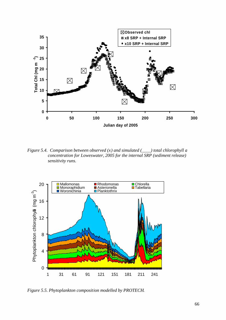
66
0
5
10
15
20
25
30
35
0 50 100 150 200 250 300
Julian day of 2005
Tota
l Chl
(mg
m-3
)Observed chlx8 SRP + Internal SRPx10 SRP + Internal SRP
Figure 5.4. Comparison between observed (x) and simulated (____) total chlorophyll a concentration for Loweswater, 2005 for the internal SRP (sediment release) sensitivity runs.
0
4
8
12
16
20
1 31 61 91 121 151 181 211 241
Phy
topl
ankt
on c
hlor
ophy
ll a (m
g m
-3)
Mallomonas Rhodomonas ChlorellaMonoraphidium Asterionella TabellariaWoronichinia Planktothrix
Figure 5.5. Phytoplankton composition modelled by PROTECH.

67
5.3 Modelled scenarios
Despite some imperfections in the model, and possibly also the driving data, PROTECH
seemed to be capturing the main features of algal growth in Loweswater. In the next step the
internal SRP re-cycling during summer anoxia was kept in the model and the different load
scenarios produced by GWLF were used to drive PROTECH (Table 4.10).
0
5
10
15
20
25
30
0 50 100 150 200 250 300Julian Day
Phy
topl
ankt
on c
hlor
ophy
ll a
(mg
m-3
)
AB
CDE
F
Figure 5.6. PROTECH simulation of phytoplankton chlorophyll a for the different SRP load
scenarios quantified in Table 4.10.
Figure 5.6 shows that algal growth in the early spring is not controlled by the availability of
phosphorus: instead physical factors such as light, temperature and flushing rate, are likely to
be the main controlling factors. For the rest of the year the availability of phosphorus
controlled the amount of phytoplankton in the lake, particularly in the autumn when the
phytoplankton were strongly controlled by the availability of phosphorus.

68
y = 0.024x + 8.159R2 = 0.988
8
9
10
11
12
13
0 50 100 150 200SRP load (kg y-1)
Ave
rage
phy
topl
ankt
on c
hl a
(mg
m-3
)
A: landcover only
B: Landcover plus slurry
C: Landcover plus septic tanks OK
E: Landcover plus slurry plus septic
tanks OK
D: Landcover plus non-functioning septic tanks
F: Landcover plus slurry plus non-
functioning septic tanks
Figure 5.7. Average phytoplankton chlorophyll a concentration between Julian days 1 and
257 modelled by PROTECH as a function of SRP loads for the six scenarios.
One way of summarising the outputs of the PROTECH modelling exercise is to calculate the
average phytoplankton chlorophyll a concentration and relate this to the annual SRP loads
derived from GWLF as presented in Table 4.10. The result of this is shown in Figure 5.7.
Again, the response highlights the fact that increasing phosphorus loads leads to increased
phytoplankton biomass, i.e. phosphorus is the nutrient limiting phytoplankton production.
Scenario E provides the best guess of the current loading situation for Loweswater. It assumes
that all of the septic tanks in the catchment were well maintained. If this were not the case,
then a much larger load of SRP would reach the lake with a proportionate increase in
phytoplankton. Scenario C assumes that none of the waste from the animal husbandry was
reaching the lake, in contrast to Scenario E. This would have a relatively large effect on SRP
load and phytoplankton productivity, with a predicted reduction in phytoplankton chlorophyll
a of about 12%. In contrast, the effect of septic tanks in the catchment, if they are all
functioning properly, is relatively small and adds little to the SRP load or the phytoplankton
biomass over that produced by losses of SRP from the land.

69
5.4 Discussion
Modelling exercises such as these need to be treated with a large degree of caution as they are
based on a hierarchy of uncertainty that derives from the driving data themselves and
simplifications and misconceptions within the model. Nevertheless, if treated with care they
provide a useful way of assessing the response of a lake to possible future scenarios.
PROTECH was used to convert the phosphorus loads into estimates of phytoplankton
chlorophyll a. The modelling confirmed that phosphorus was the main nutrient controlling the
phytoplankton productivity. The possible management implications of these model runs are
discussed in the next section.

70
6. Summary and Conclusions
This project has been undertaken because of the desire within the Loweswater community to
improve the water quality of their lake. The project arose from efforts by the Loweswater
Improvement Project to gain recognition of the problems within the catchment and support
for their initiatives to tackle them. The National Trust, as lake owners in the catchment, are
part of the community in Loweswater and have given their support to this project in a variety
of ways (including financial support). While it has been undertaken by scientists, the project
has relied on being closely linked to the local community living and working within the
Loweswater catchment and there has been a steady flow of information between the scientists
and the community of land owners throughout the project. This has given both parties a
greater understanding of the catchment and its problems.
The monitoring work shows that Loweswater is a productive lake whose productivity is
largely controlled by the availability of phosphorus to the phytoplankton. The relatively high
productivity results in oxygen depletion at depth during the summer. There is circumstantial
evidence to suggest that this promotes the internal release of phosphorus from anoxic
sediments at depth, which is an important supplement to the phosphorus being delivered from
the catchment. This internal supply of phosphorus derives from historical inputs of
phosphorus and the magnitude of this re-cycling will determine how rapidly the lake will
recover if external loads are reduced. There is evidence from historical data that the lake
water quality started to deteriorate in the 1850s but has accelerated in the last 20 years.
Presently, the lake is meso-eutrophic but would probably fail current Water Framework
Directive criteria for good ecological status for this type of lake. As a consequence there is
likely to be pressure to improve the water quality in Loweswater.
The studies of nutrient load produced estimates of the daily load of SRP, the main available
form of phosphorus, to the lake and these were used in combination with meteorological data
to drive the lake model PROTECH. The models outputs suggested that the most obvious
management option to reduce the SRP load to the lake is to ensure that all of the septic tanks
within the catchment are well-maintained and working efficiently. The second priority option
is to reduce the amount of phosphorus reaching the lake as a result of animal husbandry. This
includes losses from slurry pits or tanks, especially when they are not roofed (and so able to
lose slurry during high rainfall) and losses resulting from slurry spreading, especially if this

71
occurs at times when there is a large potential loss to streams and hence the lake. However,
the modelling work suggests that the diffuse losses from the catchment, particularly from
improved grassland, is the major source of phosphorus to the lake. This suggests that recent
efforts to reduce the amount of phosphorus applied to the land as fertiliser is a potentially very
valuable step towards improving the water quality of the lake. Inevitably there are other
potential factors which contribute to lake processes which have not been considered in this
study, including changed management practices at the outflow end of the lake and the
possible impact of over-wintering geese, but it is likely that these currently have less impact
than the factors outlined above.
The role of the Loweswater community in this project has been very beneficial and has
opened up possibilities for new forms of integrated catchment management that involve rural
agencies and, where appropriate, scientists, but which fundamentally rely upon the
communities that live and work in those catchments. It is hoped that, given the opportunity,
CEH and colleagues at Lancaster University may be able to continue to work with the
catchment community, RDS, the EA and the Lake District National Park Authority to explore
effective catchment management in Loweswater from a social, economic and environmental
perspectives (see Appendix 2 - RELU concept note).
The work reported here has hopefully produced a better understanding of how the
Loweswater system works, the key ecological issues at Loweswater and recommends ways of
improving the water quality in the lake. We further recommend that a low-level monitoring
programme is initiated so that any improvements can be monitored or any lack of
improvement noted and further action taken. One suggestion with relatively modest cost is to
make a quarterly survey of the lake, using the methodology used in the Lakes Tour, every
year until the planned next Lake Tour, i.e. in 2010. This approach would allow comparisons
with historical data, for example as analysed in Section 3 of this report. A useful addition
would be to take an additional sample in mid-August to quantify the magnitude of oxygen
depletion in the lake.

72
7. Acknowledgements
We thank the Environment Agency for granting us access to their long term and
contemporary data; in particular, John Pinder, Andrew Booth, Susan Taylor and Val Coates.
We thank Danny & Kath Leck for undertaking the daily sampling and providing us with
information about the catchment. Mark Astley (National Trust) was also very helpful in
providing useful information. We are also grateful to the New York City Department of
Environmental Protection for allowing us to use their version of the GWLF model on the
Loweswater catchment.

73
8. References
Bailey-Watts, A.E., Sargent, R., Kirika, A., & Smith, M. (1987) Loch Leven Phosphorus
loading. Contract Report to Department of Agriculture and Fisheries, Nature
Conservancy Council. Scottish Development Department and Tayside Regional
Council.
Bennion H., Appleby P., Boyle J., Carvalho L., Luckes S. & Henderson A. (2000). Water
quality investigations of Loweswater, Cumbria. Final report to the Environment Agency
by University College London. 80pp.
Carrick T. R., and D. W. Sutcliffe (1982). Concentrations of major ions in lakes and tarns of
the English Lake District (1953-1978). FBA Occasional publication no. 16. Freshwater
Biological Association, Ambleside.
Carvalho L., Maberly S.C., May L., Reynolds C.S., Hughes M., Brazier R., Heathwaite L.,
Liu S., Hilton J., Hornby D., Bennion H., Elliott A., Willby N., Dils R., Pope L. and
Phillips G. (2004). Risk Assessment Methodology for Determining Nutrient Impacts in
Surface Freshwater Bodies. Final Report to the Environment Agency and Scottish
Environment Protection Agency. 157 pp.
Carvalho, L., Maberly, S., May, L., Reynolds, C., Hughes, M., Brazier, R., Heathwaite, L.,
Liu, S,, Hilton, J., Hornby, D., Bennion, H., Elliott, A., Willby, N., Dils, R., Pope, L.,
Fozzard, I. And Phillips, G. (2005). Risk Assessment Methodology for Determining
Nutrient Impacts in Surface Freshwater Bodies. Final R&D Technical Report P2-260/9
to the Environment Agency and Scottish Environment Protection Agency, July 2004.
171 pp.
Casey, T.J., O'Connor, P.E. & Greene, R.G. (1981). A survey of phosphorus inputs to Lough
Leane. Irish Environmental Science 1: 21-34.
Chiaudani M. & Vighi M. (1984). A simple method to estimate lake phosphorus
concentrations resulting from natural background loadings. Water Reseach 19: 987-991.

74
Cooke, G.W. & Williams, R.J.B. (1973) Significance of man-made sources of phosphorus:
fertilizers and farming. Water Research 7: 19-33.
Dillon, P.J. & Kirchner, W.B. (1975) The effects of geology and land use on the export of
phosphorus from watersheds. Water Research 9: 135-148.
George D.G., Maberly S.C. & Hewitt D.P. (2004).The influence of the North Atlantic
Oscillation on the physics, chemistry and biology of four lakes in the English Lake
District. Freshwater Biology 49: 760-774.
Haith, D. A. and Shoemaker, L. L. (1987). Generalized watershed loading functions for
stream flow nutrients. Water Resources Bulletin 23: 471-478.
Haith, D. A. and Tubbs, L. J. (1981). Watershed Loading Functions for Nonpoint Sources.
ASCE. Journal of Environmental Engineering 107(EE1):121-137.
Harper D.M. & Stewart W.D.P. (1987) The effects of land use upon water chemistry,
particularly nutrient enrichment, in shallow lowland lakes: comparative studies of three
lochs in Scotland. Hydrobiologia 148: 211-229.
Lund J.W.G., Kipling C. & Le Cren E.D. (1958). The inverted microscope method of
estimating algal numbers and the statistical basis of estimations by counting.
Hydrobiologia 11: 143-170.
Maberly S.C., King L., Dent M.M., Jones R.I. & Gibson C.E. (2002) Nutrient limitation of
phytoplankton and periphyton growth in upland lakes. Freshwater Biology 47: 2136-
2152.
Mackereth F.J.H., Heron J. & Talling J.F. (1978).Water Analysis: Some revised methods for
limnologists. Freshwater Biological Association Scientific Publication No. 36. Titus
Wilson & Son Kendal.
May, L., Place, C.J. & George, D.G. (1995) The Development of a GIS-based catchment
model to assess the effects of changes in land use on water quality. Report to National
Rivers Authority, North West Region, by Institute of Freshwater Ecology, Edinburgh
Laboratory, 21 pp., 7 Figures, 9 Tables, 2 Appendices.

75
May, L., Place, C.J. and George, D.G. (1994) The development of a GIS-based catchment
model to assess the effects of changes in land use on water quality. Report to National
Rivers Authority, NW Region, 20 pp., 7 Figures, 9 Tables, 2 Appendices.
May, L., Place, C.J., George, D.G. & McEvoy, J. (1996) An assessment of the nutrient
loadings from the catchment to Bassenthwaite Lake. Report to National Rivers
Authority, North West Region, by Institute of Freshwater Ecology, Edinburgh
Laboratory, 53 pp.
Mortimer C.H. (1941). The exchange of dissolved substances between mud and water in
lakes. I. Journal of Ecology 29: 280-329.
Mortimer C.H. (1942). The exchange of dissolved substances between mud and water in
lakes. II. Journal of Ecology 30: 147-201.
NERC AA (1999). Flood Estimation Handbook CD-ROM, Version 1.0. Centre for Ecology
and Hydrology, Wallingford.
OECD (1982). Eutrophication of Waters: monitoring, assessment and control. Technical
Report, Environmental Directorate, OECD, Paris.
Parker J.E., Abel D., Dent M.M., Fletcher J.M., Hewitt D.P., James J.B., Lawlor A.J., Lofts
S., Simon B.M., Smith E.J. & Vincent C.D. (2001). A survey of the limnological
characteristics of the lakes of the English Lake District: The Lakes Tour 2000. Report to
the Environment Agency. 60 pp.
Reynolds C.S., Irish A.E. & Elliott J.A. (2001). The ecological basis for simulating
phytoplankton responses to environmental change (PROTECH). Ecological Modelling,
140: 271-291.
Skinner J.A., Lewis K.A., Bardon K.S., Tucker P., Catt J.A., Chambers B.J. (1991). An
overview of the environmental impact of agriculture in the UK. Journal of
Environmental Management, 50: 111-128.
Talling J. F. (1999). Some English lakes as diverse and active ecosystems: a factual summary
and source book. Freshwater Biological Association, Ambleside. 80 pp.

76
Talling J.F. (1974). In standing waters. In: A Manual on Methods for Measuring Primary
Production in Aquatic Ecosystems, Ed. R.A. Vollenweider (IBP Handbook No. 12,2nd
edn), PP 119-123. Oxford, Blackwells.
Ulen B. M., Kalisky T. (2005.) Water erosion and phosphorus problems in an agricultural
catchment-Need for natural research for implementation of the EU Water Framework
Directive. Environmental Science and Policy 8: 477-484.
Walling D.E., Webb B.W. (1985). Estimating the discharge of contaminants to coastal waters
by river: Some cautionary comments. Marine Pollution Bulletin 16: 488-492.

77
9. Appendices
Appendix 1 To be attached in the paper version, or scanned in and attached in a later draft Appendix 2 Understanding and acting within Loweswater: a community approach to catchment
management
Participants PI - Claire Waterton – Institute for Environment, Philosophy and Public Policy, Lancaster University, Co-PI– Lisa Norton, Centre for Ecology and Hydrology (CEH), Lancaster Co-PI– Stephen Maberly, CEH Lancaster Co-PI – Nigel Watson, Department of Geography, Lancaster University Agreed partners – The Loweswater Project, Loweswater Parish Council, Ken Bell (Parish Council and Loweswater Project member), Rural Regeneration Cumbria, Voluntary Action Cumbria, Mike Berners-Lee (Business consultant), National Trust, Rural Development Service, Environment Agency, Lake District National Park Authority, Lake District Still Waters Partnership (LDSWP), United Utilities Scientific objectives and deliverables The proposed research directly addresses the RELU cross-cutting theme of ‘identifying appropriate mechanisms for integrating social, economic and environmental goals in monitoring and management of change’ through the main overarching objective : to generate and carry out a focused, interdisciplinary body of research, aimed towards sustainable catchment management, that involves the local community and stakeholders within a new institutional mechanism. There will be three main deliverables:
i. the creation of an institutional mechanism enabling community and stakeholder based decision-making in Loweswater;
ii. a focused, interdisciplinary body of research that involves the local community and stakeholders, to contribute towards sustainable catchment management at Loweswater
iii. mechanisms for transferring this approach to other parts of the rural landscape. Outline of proposal Ostensibly a peaceful and beautiful part of the Lake District National Park, the relatively isolated catchment and community of Loweswater is host to a number of inter-related ecological, economic and social problems. These problems are not uncommon in rural, agriculturally dependent communities and include: environmental pollution, economic crisis, dysfunctional communication and a sense of impending threat to community viability. The proposed project was made possible by the ‘Loweswater Project’, a self-generated farmer initiative to tackle pollution issues in the lake, ‘Loweswater’. The RELU scoping study ‘Understanding Loweswater’ built on this and helped to establish and extend good relationships among farmers, residents and relevant stakeholders in the catchment. Both projects recognised the potential significance of institutional flexibility at a local level and the importance of local champions in tackling rural social/environmental problems. These two projects have made it apparent that there is an opportunity in Loweswater to experiment with new institutional mechanisms around the sharing of expertise, deliberative and negotiated planning, self-organisation and social learning following many aspects of Integrated Catchment Management (ICM). Of particular interest is collaborative catchment management (Watson 2004) as seen in various programmes such as Hydrology for Life and Policy (HELP) and Social Learning for Integrated

78
Management (SLIM). The project will create relationships with initiatives in train, such as catchment initiatives under LDSWP (e.g. Bassenthwaite and Haweswater) and beyond (e.g. United Utilities SCAMP programme). The project will also draw upon and contribute to debates within science studies about the creation of new ‘collectives’ of expertise (Latour 2004) and the way in which they might inform governance and decision making. Whilst the formation of a new institutional mechanism for addressing catchment problems will itself constitute part of the research, simultaneous research ‘packages’ will also be needed to generate additional information which will enable the catchment and stakeholder community to move towards an agreed future. The previous RELU study identified that a better understanding of the catchment is needed that links land use, land quality and water quality, the economic dynamics of the catchment, the potential impacts of existing and future systems of policy and governance affecting the catchment, and an understanding of social dynamics and change within and beyond the catchment. Those within the new institutional mechanism will strive to gather together these kinds of understandings through continued integrated working of scientists and stakeholders (including organisations such as Rural Regeneration Cumbria and individual land owners in the catchment), combining quantitative and qualitative data from a range of relevant sources and using appropriate technology (e.g. GIS) to evaluate present and future options and scenarios/models. As scientists, farmers, landowners and institutional representatives begin to work together, new research questions will be generated. Following insights from the previous study the following research packages are initially deemed appropriate: Terrestrial ecology; ecosystem function – biodiversity and landscape character Loweswater is primarily a farmed catchment within the National Park in an area designated as ‘environmentally sensitive’. It is managed by a range of land-owners and demonstrates a variety of landscape features, biodiversity and management. Aims: to understand the relationships between farming and the ecological character of the catchment and to assess the ecological and farming potentials of the catchment. Methods: 1) to look at the ecology of the catchment through survey and habitat mapping, 2) to work with farmers, their advisors and governing institutions to understand how farmers ‘know’ and work with their land as well as the practical and economic constraints within which they operate and 3) to explore potential futures for land use in the catchment. Aquatic ecology; ecosystem function – water quality & conservation Research is needed that builds on work under a project funded through the Defra Rural Enterprise Scheme (04-05). That project involved monthly sampling of Loweswater and its feeder streams to identify sources of nutrient input and to supply data for a model of algal growth in the lake. Aims: to improve understanding of the impact of human activity in the catchment on water quality and fish stocks. To provide practical information to the community to help evaluate the effect of land management scenarios on water quality, fish stocks and fishing in the lake. Methods: Diffuse gel technology will be used to produce an improved estimate of phosphorus loading to the lake that captures short-term events and includes estimates from land managed in different ways. The model that is already developed will be used to evaluate scenarios of land management and nutrient input in terms of water quality. Surveys of current fish stocks will be carried out and assessed in relation to historical surveys. Local people and their local knowledge will be used in carrying out the surveys. Catchment economy Loweswater is a catchment subject to all of the current policy drivers affecting farming. As part of a National Park there are further factors impacting on the management of land and holdings. Whilst farming incomes are poor in the uplands, the Lake District is an attractive environment for retirees or second home owners which has resulted in high property and land prices. Aims: to explore the economics of the catchment in order to discover how the rural livelihoods can be made there, to see how external pressures impact on the residents of Loweswater and to look to the likely impact of economics on the community in Loweswater into the future (particularly in regard to CAP reform, tourism and land/property prices).

79
Methods: to work with the community at Loweswater and local rural economists (from Farm Connect Cumbria and Rural Regeneration Cumbria) to look at the impacts of changing policy and economy on the Loweswater catchment; to explore economic scenarios consistent with the future sustainability of the catchment. Catchment sociology and social change As part of the RELU scoping study, it was recognised that future work would need to generate a deeper understanding of the rural sociology of this catchment, including what sustains a sense of ‘community’, how the local community is connected to wider social, cultural, economic and policy (including agricultural) structures, and how these affect social/natural change within the catchment. Aims: drawing upon environmental sociology/anthropology and the sociology of knowledge, this research package aims to foster a recognition that ‘local knowledge’ about the catchment, will have significance, alongside, and for, other forms of knowledge (for example the ecological work of Norton and Maberly). The RA appointed for this part of the study will work with natural scientists as well as alongside Ken Bell, Claire Waterton and Nigel Watson (Geography) in structuring and facilitating community decision-making. Lastly, this part of the project will explore the transferability of the proposed institutional experiment to other rural social/environmental problems. Methods: desk studies/documentary analysis (understanding the sociology of Loweswater); interviews and participant observation within the catchment (drawing out local knowledge of environment and society); and facilitating interdisciplinary interactions and community decision-making. Potential policy relevance/Stakeholder engagement The work will be highly relevant to policy concerning land, water, rural communities and science-policy-community interactions. Current levels of phytoplankton chlorophyll in Loweswater are close to the ecologically poor value under the EC Water Framework Directive: improvement will require diffuse and point sources of phosphorus to be controlled by 2015. Common Agricultural Policy reform and the introduction of the Single Farm Payment require that land is kept in Good Agricultural Environmental Condition and refers to potential impacts of land management on water quality. The potential impact of CAP reform on marginal upland hill farms is currently a matter for concern. The implementation of i) the government’s Rural Strategy (2004) aimed at development/enhancement of rural economies and ii) Regional and Local Framework Development Plans to complement Parish Plans are also highly relevant. This project is well advanced in terms of stakeholder engagement. The ‘Loweswater Project’ will remain a central body of stakeholders. The Parish Council have shown support for the project following public consultation. RDS and the EA have already committed funds and goodwill towards the proposed research (see below). The LDSWP have given their backing and have agreed to share experiences from Bassenthwaite and Haweswater catchment management initiatives. The National Trust who own the lake and land in the catchment are involved and have contributed funding to projects aimed at improving the catchment (see below). Both Rural Regeneration Cumbria and Voluntary Action Cumbria have been consulted and expressed interest in providing their expertise in line with project aims. Approach to interdisciplinarity This work will build on well-established interdisciplinary social/natural science partnerships between researchers based at the Lancaster Environment Centre. Interdisciplinarity is central to the PI’s work in the sociology of the environment, environmental knowledge and policy-making. This proposal to bring together different forms of expertise within a new community-based collective signals a willingness to experiment with disciplinary integration with a practical aim - to help solve policy and land-use problems at Loweswater. References: Latour, B. (2004) Politics of Nature: How to bring the sciences into Democracy. Cambridge, Mass: Harvard University Press. Watson, N. (2004) Integrated river basin management: A case for collaboration, International Journal of River Basin Management, Volume 2 (3), pp.1-15. Defra Rural Strategy (2004) http://www.defra.gov.uk/rural/strategy/default.htm