an investigation of a flat plate oscillating heat pipe …

AN INVESTIGATION OF A FLAT PLATE OSCILLATING HEAT PIPE AS A THERMAL SPREADER WITH CENTERED HEATING

A Thesis Presented to the Graduate School

University of Missouri-Columbia

In Partial Fulfillment of the Requirements for the Degree:

Master of Science

Author:

AARON T. JOHNSON

Dr. Hongbin Ma, Thesis Supervisor

May 2015

The undersigned, appointed by the Dean of the Graduate School, have examined the thesis

entitled

AN INVESTIGATION OF A FLAT PLATE OSCILLATING HEAT PIPE AS A THERMAL SPREADER WITH CENTERED HEATING

Presented by Aaron T. Johnson

A candidate for the degree of Master of Science

And hereby certify that in their opinion it is worthy of acceptance.

_____________________________________ Hongbin Ma

_____________________________________ Yuwen Zhang

____________________________________Stephen Montgomery-Smith

ii

Acknowledgements

I must thank my mother and father for this achievement: Mom for showing me

that I must always pursue a goal and Dad for showing me that there is always a process

that will attain the goal. Without their combined guidance, I never would have made it as

far as I have.

I also thank Dr. Ma for putting up with me, as I know I was not always the easiest

student to deal with. I also thank him for giving me an understanding of heat pipes and

thermal engineering that I imagine few will be able to rival as I head into industry.

I must also acknowledge the contributions of others to this work. Scott

Thompson, Aaron Hathaway, Hanwen Lu, Fritz Laun, and Corey Wilson all were

instrumental in me being able start, set up, and finish this investigation. Without their

continued patience and advice, it would have been far more difficult to achieve.

iii

Table of Contents

Acknowledgements…….….……….…………………………………………………..….ii

List of Figures…….….……………….………………………………………………..…iv

List of Tables………….…….………………...…………………….……………………vi

Nomenclature…………………………………..………………………….…………….vii

Abstract………...……..…………………….………………………………………….…xi

Chapter 1: Introduction and Literature Review……………………...……………….…...1

Chapter 2: Mathematical Model..........................................................................................9

2.1 Approach………………………………………………………………………9

2.2 Continued Approach with Application………………………………...…….17

Chapter 3…………………………………………………………………………………23

3.1 Experimental Setup………………………………………………………….23

3.2 Procedure……………………………………………………………….…...30

3.3 Uncertainty Analysis………………………………………………………..31

Chapter 4: Results and Discussion……………………………………………………….34

Chapter 5: Conclusion………………………………………………….………………..45

References…………………………………………………………………………….….46

Appendix A: Presented Graphs of all steady state temperature distributions...…………47

Appendix B: Matlab Code used for Computation………………...…………………….60

Appendix C: Uncertainty Equations Presented in order of calculation………………....65

iv

List of Figures

Figure 1.1 Basic depiction of an oscillating heat pipe, axial configuration.

Figure 1.2 Basic depiction of an oscillating heat pipe, spreader configuration.

Figure 2.1 Basic depiction of the thermal resistance network.

Figure 2.2 Schematic of heat spreader embedded with flat plate oscillating heat pipe.

Figure 2.3 Thermal resistance varied against the thermal conductivity while h is held constant at 150 W/m^2 K

Figure 2.4 Convection Coefficient varied while holding k constant at 1000 W/m^2 K.

Figure 2.5 Initial computed results plotted. Predictions indicate reasonable values of surface temperature T.

Figure 3.1 Drawing of the actual heat pipe

Figure 3.2 Photo of the heat pipe, pre brazing.

Figure 3.3 Photo of experimental setup.

Figure 3.4 Topside view of setup showing flow pattern and thermocouple

Figure 3.6: Block diagram of experimental setup.

Figure 4.1: Graph taken from Thompson et al. [10] showing experimentally obtained values.

Figure 4.2: Graph of calculated or predicted surface temperatures of the heatpipe/heat sink for experiment 2

Figure 4.3: Graph of calculated or predicted surface temperatures of copper substrate/heat sink for experiment 2.

Figure 4.4 Graph of calculated and experimental surface temperatures 1 m/s for experiment 3.



v

Figure 4.7 Graph of 9 thermocouples at 225 W and 3 m/s showing S.S. temperature distribution

Figure 4.8 Graph of 9 thermocouples at 100 W and 2 m/s showing S.S. temperature distribution

vi

List of Tables

Table 3.1 List of Equipment shown in Photograph

Table 4.1 Calculated and Experimental Thermal Resistances for Experiment 1

Table 4.2 Calculated and Experimental Thermal Resistances for heat pipe Experiment 2

Table 4.3 Calculated and Experimental Thermal Resistances for copper substrate Experiment 2

Table 4.4 Calculated and Experimental Thermal Resistances for Experiment 3

vii

Nomenclature

A = Area (m2)

a = Length of base in x-direction (m)

B = Bias Uncertainty

b = Width of base in y-direction (m)

Biot∙ 𝜏 = Dimensionless product of Biot number and τ

Bo = Bond number

C = Constant used to calculate Reynold’s number

c = Specific heat capacity (J/kg K)

D = Diameter (m)

g = Acceleration of gravity (m/s2)

H = Height of fin (m)

h = Convection coefficient (Watts/m2 K)

I = Input Current (Watts)

J = Input Voltage (volts)

k = Conduction coefficient (Watts/m K)

= Mass flow rate (kg/s)

N = Number of fins

viii

𝑁𝑢 𝐷 = Nusselt number

P = Perimeter (m)

p = Substrate aspect ratio

Pr = Dimensionless Prandtl number

Q = Heat input (Watts)

R = Resistance (°C/Watt)

𝑅𝑒𝐷 = Reynold’s number

T = Temperature (°C)

t = Thickness of plate (m)

U = Total combined bias and precision uncertainty

u = Uncertainty

V = Velocity (m/s)

W = Precision uncertainty

z = standard deviation

Greek Symbols

α = Dimensionless source width

β = Dimensionless source length

δ = Dirac delta function

μ = Kinematic viscosity (m2/s)

ix

ρ = Density (kg/m3)

σ = Surface tension (N/m)

τ = Dimensionless plate thickness

φ = Fourier coefficients for heat source

Ψ = Thermal resistance (°C/Watt)

ψ = Fourier coefficients for temperature distribution

Subscripts

c = Condenser

e = Evaporator

eff = Effective

f = Fin

l = Summation index

liq = Liquid

m = Summation index

sp = Spreading

T = Temperature

t = total

u = Sum of conductive and convective

x

vap = Vapor

∞ = Ambient

xi

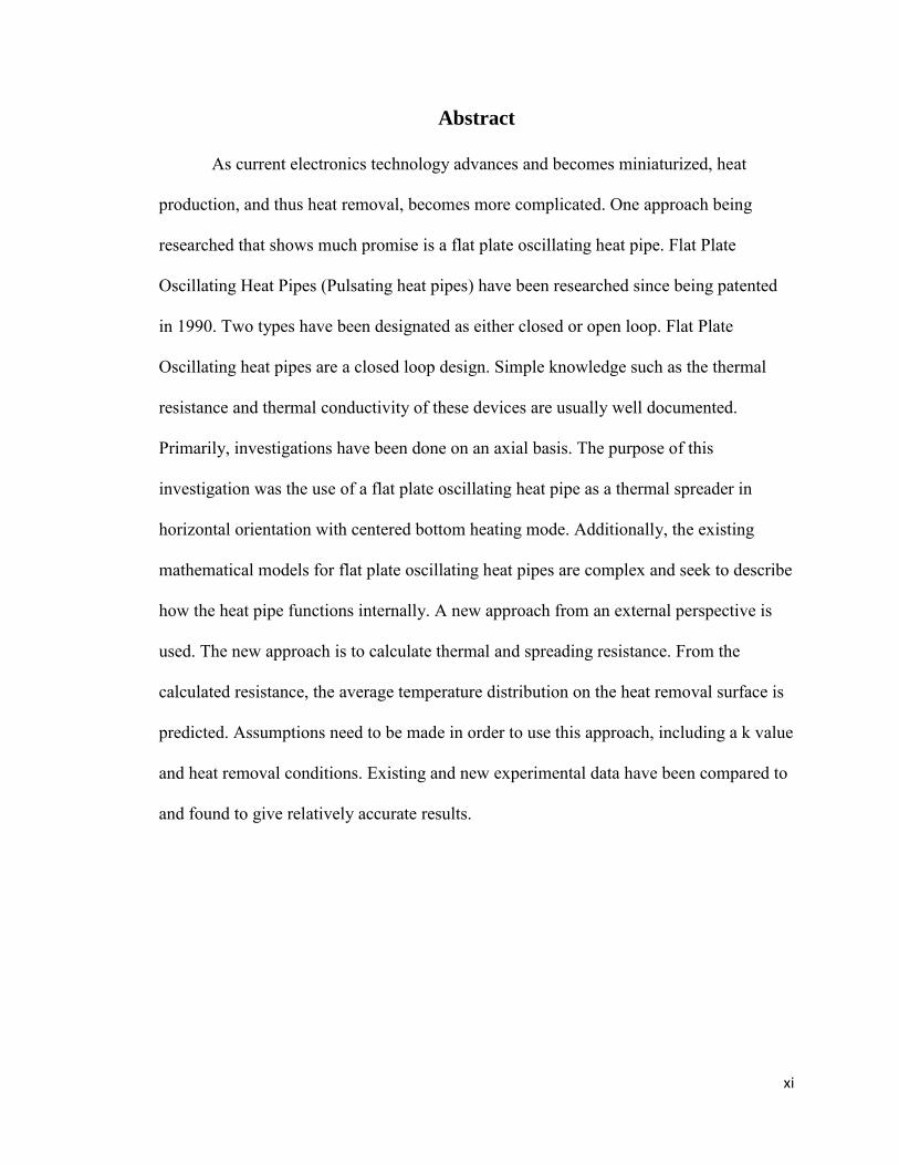
Abstract

As current electronics technology advances and becomes miniaturized, heat

production, and thus heat removal, becomes more complicated. One approach being

researched that shows much promise is a flat plate oscillating heat pipe. Flat Plate

Oscillating Heat Pipes (Pulsating heat pipes) have been researched since being patented

in 1990. Two types have been designated as either closed or open loop. Flat Plate

Oscillating heat pipes are a closed loop design. Simple knowledge such as the thermal

resistance and thermal conductivity of these devices are usually well documented.

Primarily, investigations have been done on an axial basis. The purpose of this

investigation was the use of a flat plate oscillating heat pipe as a thermal spreader in

horizontal orientation with centered bottom heating mode. Additionally, the existing

mathematical models for flat plate oscillating heat pipes are complex and seek to describe

how the heat pipe functions internally. A new approach from an external perspective is

used. The new approach is to calculate thermal and spreading resistance. From the

calculated resistance, the average temperature distribution on the heat removal surface is

predicted. Assumptions need to be made in order to use this approach, including a k value

and heat removal conditions. Existing and new experimental data have been compared to

and found to give relatively accurate results.

1

Chapter 1

Introduction and Literature Review

Current electronics cooling technologies are fast approaching a limit. With each

iteration of electronic devices, either the power density is increased or the package

becomes smaller. These can lead to increased thermal management issues. Currently

employed low-cost heating solutions such as heat sinks, with or without a traditional heat

pipe, will soon be unable to handle the heat load effectively. There are many new

technologies under investigation to become the next generation of thermal management

device. One such device was invented and patented in 1990 by Akachi [1]. He describes

a structure in which only a liquid and its vapor phase are present separated into a train of

liquid plugs and vapor bubbles. In this structure, the vapor bubble completely blocks the

liquid from flowing past it, provided the hydraulic diameter is small enough to provide

such a formation. The hydraulic diameter must be small enough that the liquid can form a

complete meniscus: without it, the device won’t function. It is governed by the critical

Bond number, which is usually found to be from 1.84 to 2. A typical structure has a

condenser for heat removal, an evaporator for heat addition, and an adiabatic (no heat

transfer) region. This structure also proceeds in a serpentine manner in which the tubing

used crosses the evaporator and condenser regions multiple times. It is more commonly

known as an oscillating heat pipe (OHP) and is shown in Figure 1.1.

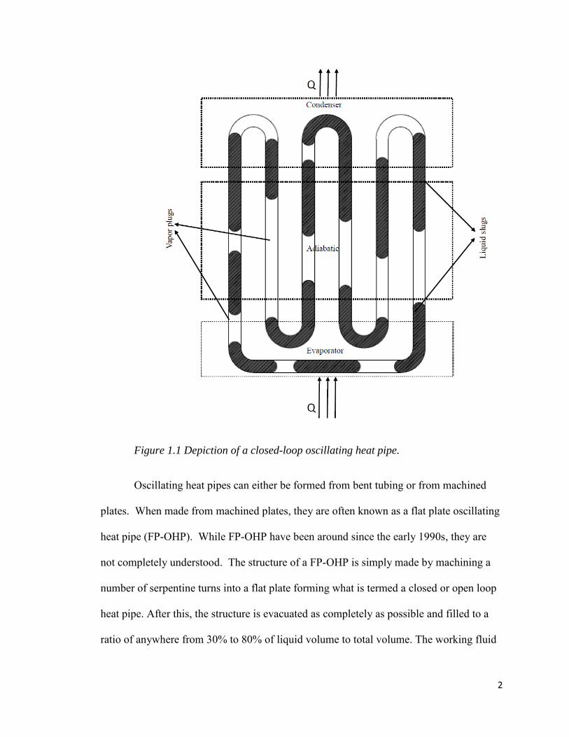
2

Figure 1.1 Depiction of a closed-loop oscillating heat pipe.

Oscillating heat pipes can either be formed from bent tubing or from machined

plates. When made from machined plates, they are often known as a flat plate oscillating

heat pipe (FP-OHP). While FP-OHP have been around since the early 1990s, they are

not completely understood. The structure of a FP-OHP is simply made by machining a

number of serpentine turns into a flat plate forming what is termed a closed or open loop

heat pipe. After this, the structure is evacuated as completely as possible and filled to a

ratio of anywhere from 30% to 80% of liquid volume to total volume. The working fluid

3

then disperses randomly into a number of vapor plugs and liquid slugs. Upon the

application of heat, these vapor bubbles expand in the evaporator section and move to the

condenser section, where they contract. The pressure change between the condenser and

evaporator results in an oscillatory motion.

There are several limiting factors such as the critical Bond number, the number of

turns, the effect of gravity, and orientation. In earlier literature, it has been suggested that

FP-OHPs are incapable of operating in a horizontal position [2] efficiently while gravity

has a significant effect on the thermal performance. Charoensawan et al [3] explored the

effects of the critical number of turns, inclination angle, working fluid, and internal

diameter. It is indicated that the critical number of turns for a device of 2 mm diameter is

about 16 for the working fluids tested, while the smaller 1 mm diameter requires more.

The paper also states that the critical number of terms depends on the working fluid and

size of the capillary tubes used, and may also depend on the input heat flux. The effect

of gravity is investigated and shown to have a generally positive effect up until around 60

degrees. However, this is in an axial configuration, with a clearly delineated evaporator at

one end and a condenser at the other. Chien et. al. [4] also investigated various filling

ratios and inclinations. However, here it was hypothesized and tested that uniform

chambers and non-uniform chambers together would provide the increased perturbations

needed for horizontal operation. It did enhance heat transfer and allowed horizontal

operation with only 8 turns as opposed to the 16 turns needed by Charoensawan et al.

[3], still using an axial configuration.

Charoensawan and Terdtoon [5, 6] have a series of papers where they

parametrically investigate several of what are termed horizontal closed loop oscillating

4

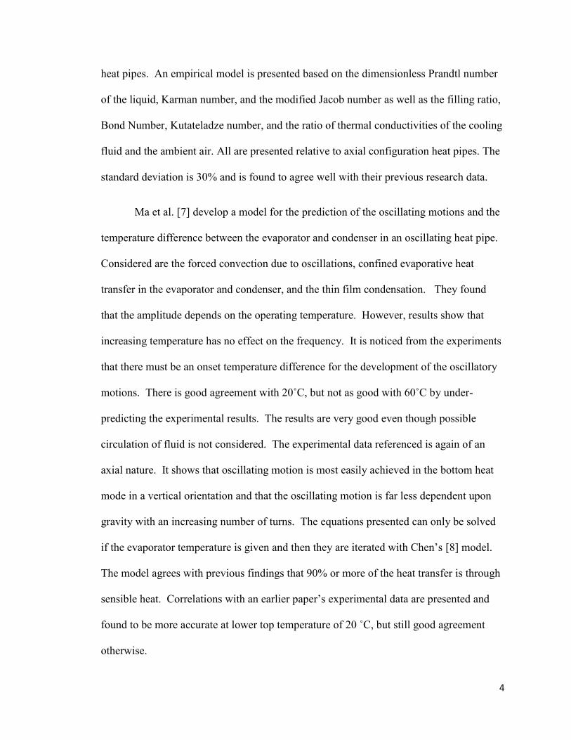
heat pipes. An empirical model is presented based on the dimensionless Prandtl number

of the liquid, Karman number, and the modified Jacob number as well as the filling ratio,

Bond Number, Kutateladze number, and the ratio of thermal conductivities of the cooling

fluid and the ambient air. All are presented relative to axial configuration heat pipes. The

standard deviation is 30% and is found to agree well with their previous research data.

Ma et al. [7] develop a model for the prediction of the oscillating motions and the

temperature difference between the evaporator and condenser in an oscillating heat pipe.

Considered are the forced convection due to oscillations, confined evaporative heat

transfer in the evaporator and condenser, and the thin film condensation. They found

that the amplitude depends on the operating temperature. However, results show that

increasing temperature has no effect on the frequency. It is noticed from the experiments

that there must be an onset temperature difference for the development of the oscillatory

motions. There is good agreement with 20˚C, but not as good with 60˚C by under-

predicting the experimental results. The results are very good even though possible

circulation of fluid is not considered. The experimental data referenced is again of an

axial nature. It shows that oscillating motion is most easily achieved in the bottom heat

mode in a vertical orientation and that the oscillating motion is far less dependent upon

gravity with an increasing number of turns. The equations presented can only be solved

if the evaporator temperature is given and then they are iterated with Chen’s [8] model.

The model agrees with previous findings that 90% or more of the heat transfer is through

sensible heat. Correlations with an earlier paper’s experimental data are presented and

found to be more accurate at lower top temperature of 20 ˚C, but still good agreement

otherwise.

5

Khandekar et al. [9] explored the effect of a number of parameters such as

inclination angle, thermo-physical properties of the working fluid, the inner tube

diameter, the number of turns, and the evaporator length in an attempt to come up with an

empirical model. They added a Karman number, defined from non-dimensional numbers

of interest, which is considered to be a suitable velocity scale for closed loop pulsating

heat pipes (CLPHP). The effect of inclination and thermo-hydrodynamic boundary

conditions were considered. However, here it is again noted that it is only an axial flow.

Khandekar and Groll [10] conducted a review of what CLPHP are with conditions. It is

suggested that a large number of turns and a high input heat flux are necessary for

horizontal CLPHP performance. It is also shown that there is a minimum heat flux or

temperature needed for a successful startup which is lowered by a larger number of turns,

though it is shown that bottom heating mode requires less power than top heating mode.

Thermal resistance decreases with increasing heat input until it is limited by heat removal

on air side. CLPHPs do not operate outside of the range of 20% to 80% filling ratios:

Sensitivity decreases with more heat input. It is also suggested that CLPHP can be

studied with an effective thermal conductivity approach, at least to a certain extent. It is

notable that thermal spreading is still not considered.

Khandekar and Groll [10] gave a background of modeling attempts. Listed are

what is termed Type I, II, III, IV, V, and VI modeling approaches. Type I starts with a

single spring mass approach, type II is a system of spring mass approach, type III applies

conservation approaches to slug-plug flow, type IV analysis highlights the existence of

chaos in some approaches, type V uses artificial neural network modeling, and type VI is

semi-empirical modeling. All of these approaches have some success, but with the

6

exception of type VI, they are limited because of extreme simplification. That is to say,

they don’t represent true thermo-fluidic behavior. The last approach is still under

investigation. Khandekar et al. [10] analyzed other similar passive heat transfer systems

in an attempt to explain CLPHP behavior better. Conventional two phase flow modeling

is attempted with estimations of each necessary parameter. This allows effective thermal

resistance with appropriate correlations in the evaporator and condenser of the device.

However, it is further limited in that it only considers two phase flow conditions in axial

configuration and cannot handle a horizontal (non-gravity assisted) configuration. The

paper does admit there are limitations to the model presented and that this paper is only a

stepping-stone to discover the true operation of CLPHPs.

Thompson et al. [11] explored a three dimensional FPOHP in centered bottom

heating mode. This means that the heat pipe presented for performance evaluation is

positioned parallel to the ground with the heat source on the bottom center. The thermal

performance in regards to thermal spreading is presented. Thermal resistance is

calculated from experimental data. The three dimensional FPOHP is explored in

increments of 10 watts from 25 Watts at 1 m/s air velocity until its maximum input of

230 watts at an air flow velocity of 3 m/s. It is compared with a copper slab control to

verify any change in performance. While there isn’t much of a change, it is noted that as

air flow velocity increases, there is a 10 to 15 percent reduction in surface temperatures,

indicating the air flow affects the FPOHP performance.

These studies generally investigated how an oscillating heat pipe functions and

what the governing parameters are. While not all directly pertinent to the current

investigation, they do provide some useful guiding parameters. For a given working fluid,

7

a specific diameter is needed as defined by the Bond number. In order to operate in the

horizontal position, a large number of turns (as well as a large input heat flux) are needed

where more is generally better. While nearly any material can be used to make a FPOHP,

copper and aluminum are both easier to machine and give better performance than such

materials as glass or plastics. Generally, the thermal conductivity order of magnitude

should be fairly well known. However, most of these configurations are tested using

clearly defined condenser and evaporator regions but only in axial configurations.

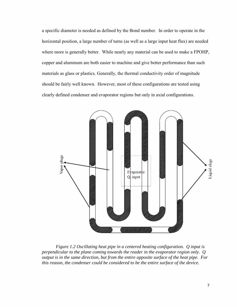
Figure 1.2 Oscillating heat pipe in a centered heating configuration. Q input is

perpendicular to the plane coming towards the reader in the evaporator region only. Q

output is in the same direction, but from the entire opposite surface of the heat pipe. For

this reason, the condenser could be considered to be the entire surface of the device.

8

Of primary interest to this investigation is a FPOHP in bottom centered heating

mode, generally known as a thermal spreading configuration. Many devices are often

more practically run with a thermal spreading configuration. Not the least of these is a

typical computer configuration with a heat sink. The chip generally is presented centered

below the heat sink generating a known heat flux, Q. In terms of FPOHP, this leads to a

very clearly defined evaporator region, but the condenser region and adiabatic regions

aren’t so well known and may very well be the same geometrically defined region.

Figure 1.2 shows such a configuration. Also of primary interest to this investigation is

whether the temperature difference can be accurately predicted through mathematical and

experimental means. This would be a welcome step towards actually being able to

design for specific needs. The models thus presented generally are concerned with the

interior physics, start up condition, time to start up, etc. They are very complex and often

of impractical value for those interested in designing a FPOHP for specific needs. The

heat pipe to be investigated here will be as a thermal spreading FPOHP in centered

bottom heating configuration. Specifically, whether or not it is possible to predict the

upper surface temperature and thus a possible maximum output.

9

Chapter 2

Mathematical Model

2.1 Approach

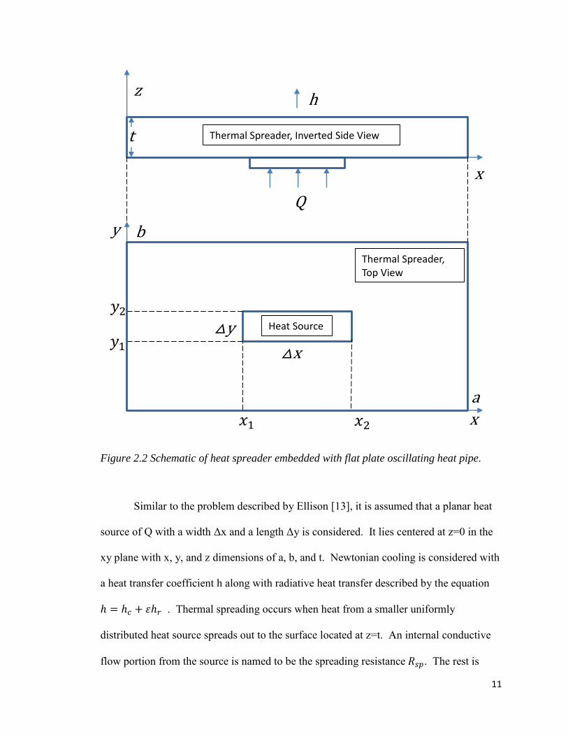
Many models have been attempted with varying degrees of success to predict how

an oscillating heat pipe (OHP) functions. Zhang and Fahgri [12] listed over 50 papers in

an attempt to update and outline the issues still concerning the knowledge of oscillating

heat pipes, many of which attempted mathematical models. These models generally have

two things in common: They try to predict the performance or physics inside of the heat

pipe and not many of them are practical from an industrial standpoint as they are very

complex. These models can be useful in understanding the governing parameters of an

OHP. The OHP must generally have a large number of turns in order to overcome

gravitational effect problems. Surface tension must dominate gravitational forces; to that

end the diameter must have a certain critical value met which is governed by the Bond

number. Generally speaking, the measured thermal resistance is between 0.03 K/W and

0.08 K/W. To this end, a simple resistance network is proposed as outlined in Fig. 2.1.

10

Figure 2.1 Basic depiction of the thermal resistance network.

Conductive and convective resistances are well known and there are many useful

models to calculate them based on geometry, flow patterns of cooling fluid, etc.

However, thermal spreading is a phenomenon which has generally been well

documented, but isn’t particularly easy to model. Ellison [13] obtained an exact solution

to this issue for rectangular plates with centered heat sources with non-unity aspect ratios.

A FPOHP with centered heating is similar to the one investigated by Ellison [13]. The

difference is that a constant thermal conductivity is assumed for the FPOHP. Following

the procedure described by Ellison [13], the physical model as shown in Fig. 2.2 is

established.

𝑇𝑠𝑜𝑢𝑟𝑐𝑒 𝑇∞

Conductive and

Convective Resistance 𝑅𝑈

Spreading Resistance 𝑅𝑠𝑝

11

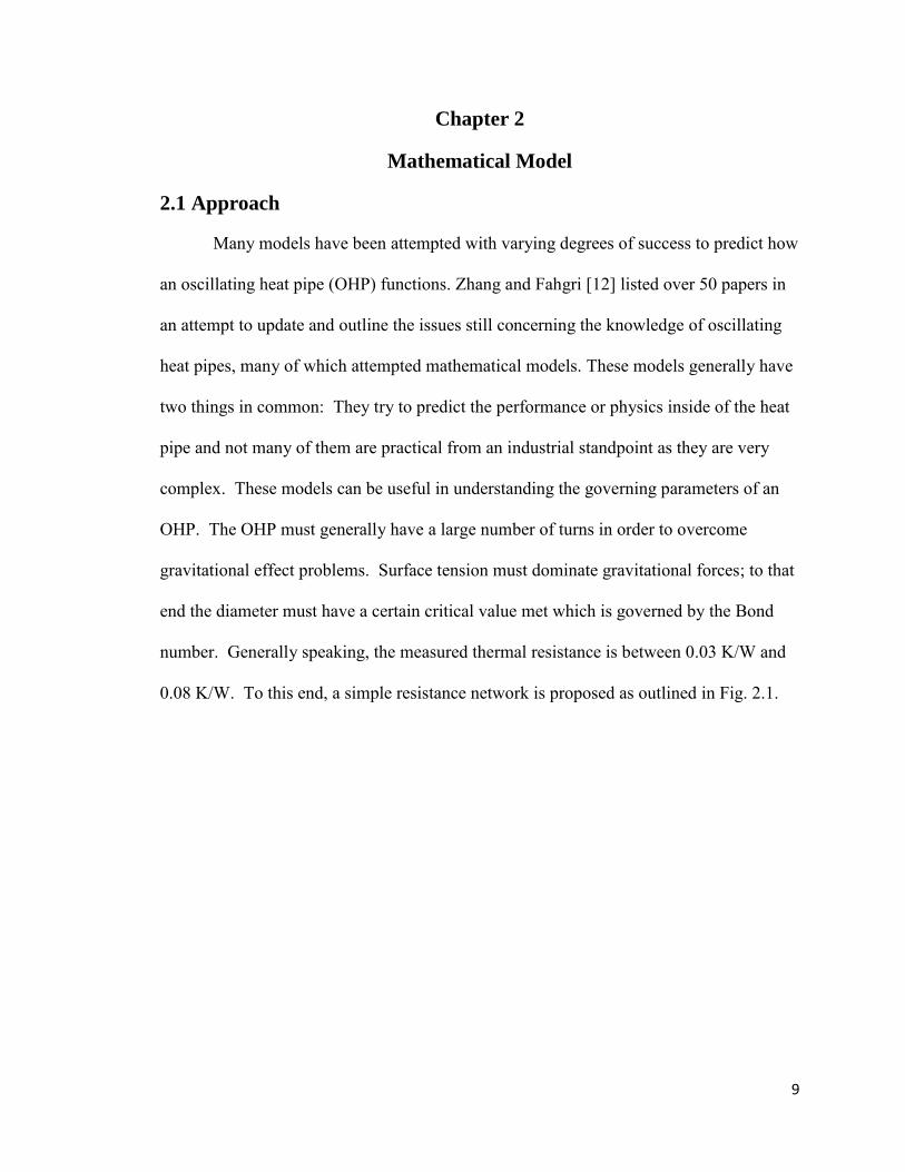
Figure 2.2 Schematic of heat spreader embedded with flat plate oscillating heat pipe.

Similar to the problem described by Ellison [13], it is assumed that a planar heat

source of Q with a width Δx and a length Δy is considered. It lies centered at z=0 in the

xy plane with x, y, and z dimensions of a, b, and t. Newtonian cooling is considered with

a heat transfer coefficient h along with radiative heat transfer described by the equation

ℎ = ℎ𝑐 + 휀ℎ𝑟 . Thermal spreading occurs when heat from a smaller uniformly

distributed heat source spreads out to the surface located at z=t. An internal conductive

flow portion from the source is named to be the spreading resistance 𝑅𝑠𝑝. The rest is

Q

h

t

z

x

x

a

y

x

𝑥1 𝑥2

𝑦1

𝑦2

y

Thermal Spreader, Inverted Side View

Heat Source

Thermal Spreader, Top View

b

12

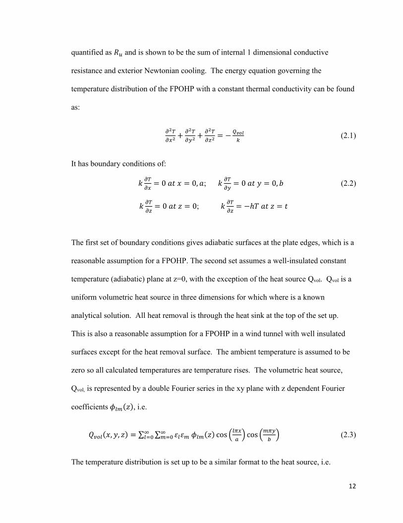
quantified as 𝑅𝑢 and is shown to be the sum of internal 1 dimensional conductive

resistance and exterior Newtonian cooling. The energy equation governing the

temperature distribution of the FPOHP with a constant thermal conductivity can be found

as:

𝜕2𝑇

𝜕𝑥2+

𝜕2𝑇

𝜕𝑦2+𝜕2𝑇

𝜕𝑧2= −

𝑄𝑣𝑜𝑙

𝑘 (2.1)

It has boundary conditions of:

𝑘𝜕𝑇

𝜕𝑥= 0 𝑎𝑡 𝑥 = 0, 𝑎; 𝑘 𝜕𝑇

𝜕𝑦= 0 𝑎𝑡 𝑦 = 0, 𝑏 (2.2)

𝑘𝜕𝑇

𝜕𝑧= 0 𝑎𝑡 𝑧 = 0; 𝑘 𝜕𝑇

𝜕𝑧= −ℎ𝑇 𝑎𝑡 𝑧 = 𝑡

The first set of boundary conditions gives adiabatic surfaces at the plate edges, which is a

reasonable assumption for a FPOHP. The second set assumes a well-insulated constant

temperature (adiabatic) plane at z=0, with the exception of the heat source Qvol. Qvol is a

uniform volumetric heat source in three dimensions for which where is a known

analytical solution. All heat removal is through the heat sink at the top of the set up.

This is also a reasonable assumption for a FPOHP in a wind tunnel with well insulated

surfaces except for the heat removal surface. The ambient temperature is assumed to be

zero so all calculated temperatures are temperature rises. The volumetric heat source,

Qvol, is represented by a double Fourier series in the xy plane with z dependent Fourier

coefficients 𝜙𝑙𝑚(𝑧), i.e.

𝑄𝑣𝑜𝑙(𝑥, 𝑦, 𝑧) = ∑ ∑ 휀𝑙휀𝑚 𝜙𝑙𝑚(𝑧) cos (𝑙𝜋𝑥

𝑎) cos (

𝑚𝜋𝑦

𝑏)∞

𝑚=0∞𝑙=0 (2.3)

The temperature distribution is set up to be a similar format to the heat source, i.e.

13

𝑇(𝑥, 𝑦, 𝑧) = ∑ ∑ 휀𝑙휀𝑚 𝜓𝑙𝑚(𝑧) cos (𝑙𝜋𝑥

𝑎) cos (

𝑚𝜋𝑦

𝑏)∞

𝑚=0∞𝑙=0 (2.4)

Shown below are the source Fourier coefficients derived for adiabatic edge boundary

conditions. They are made easier to solve via the assumption of a uniform heat flux

q(x,y) at the z=0 plate surface using the Dirac delta function δ(z) such that

Q(x,y,z)=q(x,y) δ(z). This results in

𝜙00 =4

𝑎𝑏∫ ∫ 𝑄𝑣𝑜𝑙𝑑𝑥𝑑𝑦

𝑦=𝑏

𝑦=0

𝑥=𝑎

𝑥=0

=4

𝑎𝑏𝑞(𝑥, 𝑦)𝛿(𝑧)(𝑥2 − 𝑥1)(𝑦2 − 𝑦1) (2.5)

𝜙𝑙0 =4

𝑎𝑏∫ ∫ 𝑄𝑣𝑜𝑙𝑐𝑜𝑠 (

𝑙𝜋𝑥

𝑎) 𝑑𝑥𝑑𝑦

𝑦=𝑏

𝑦=0

𝑥=𝑎

𝑥=0

=4

𝑙𝜋𝑏𝑞(𝑥, 𝑦)𝛿(𝑧)(𝑦2 − 𝑦1) [sin (

𝑙𝜋𝑥2

𝑎) − sin (

𝑙𝜋𝑥1

𝑎)] (2.6)

𝜙0𝑚 =4


𝑚𝜋𝑦

𝑏)𝑑𝑥𝑑𝑦

𝑦=𝑏

𝑦=0

𝑥=𝑎

𝑥=0

=4

𝜋𝑚𝑎𝑞(𝑥, 𝑦)𝛿(𝑧)(𝑥2 − 𝑥1) [sin (

𝑚𝜋𝑦2

𝑏) − sin (

𝑚𝜋𝑦1

𝑏)] (2.7)

𝜙𝑙𝑚 =4


𝑙𝜋𝑥

𝑎) 𝑐𝑜𝑠 (

𝑚𝜋𝑦

𝑏)𝑑𝑥𝑑𝑦

𝑦=𝑏

𝑦=0

𝑥=𝑎

𝑥=0

=4

𝜋2𝑙𝑚𝑞(𝑥, 𝑦)𝛿(𝑧) [sin (

𝑙𝜋𝑥2

𝑎) − sin (

𝑙𝜋𝑥1

𝑎)] [sin (

𝑚𝜋𝑦2

𝑏) − sin (

𝑚𝜋𝑦1

𝑏)] (2.8)

14

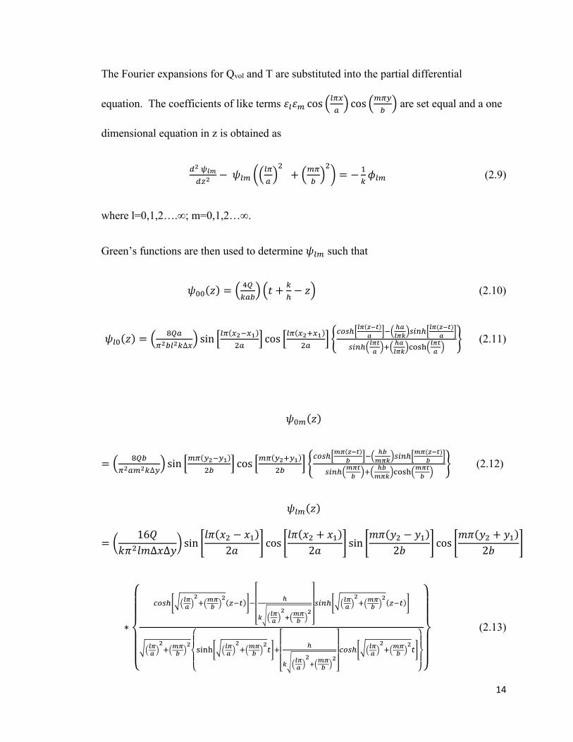
The Fourier expansions for Qvol and T are substituted into the partial differential

equation. The coefficients of like terms 휀𝑙휀𝑚 cos (𝑙𝜋𝑥

𝑎) cos (

𝑚𝜋𝑦

𝑏) are set equal and a one

dimensional equation in z is obtained as

𝑑2 𝜓𝑙𝑚

𝑑𝑧2− 𝜓𝑙𝑚 ((

𝑙𝜋

𝑎)2

+ (𝑚𝜋

𝑏)2

) = −1

𝑘𝜙𝑙𝑚 (2.9)

where l=0,1,2….∞; m=0,1,2…∞.

Green’s functions are then used to determine 𝜓𝑙𝑚 such that

𝜓00(𝑧) = (4𝑄

𝑘𝑎𝑏) (𝑡 +

𝑘

ℎ− 𝑧) (2.10)

𝜓𝑙0(𝑧) = (8𝑄𝑎

𝜋2𝑏𝑙2𝑘∆𝑥) sin [

𝑙𝜋(𝑥2−𝑥1)

2𝑎] cos [

𝑙𝜋(𝑥2+𝑥1)

2𝑎]

𝑐𝑜𝑠ℎ[𝑙𝜋(𝑧−𝑡)

𝑎]−(

ℎ𝑎

𝑙𝜋𝑘)𝑠𝑖𝑛ℎ[

𝑙𝜋(𝑧−𝑡)

𝑎]

𝑠𝑖𝑛ℎ(𝑙𝜋𝑡

𝑎)+(

ℎ𝑎

𝑙𝜋𝑘)cosh (

𝑙𝜋𝑡

𝑎)

(2.11)

𝜓0𝑚(𝑧)

= (8𝑄𝑏

𝜋2𝑎𝑚2𝑘∆𝑦) sin [

𝑚𝜋(𝑦2−𝑦1)

2𝑏] cos [

𝑚𝜋(𝑦2+𝑦1)

2𝑏]

𝑐𝑜𝑠ℎ[𝑚𝜋(𝑧−𝑡)

𝑏]−(

ℎ𝑏

𝑚𝜋𝑘)𝑠𝑖𝑛ℎ[

𝑚𝜋(𝑧−𝑡)

𝑏]

𝑠𝑖𝑛ℎ(𝑚𝜋𝑡

𝑏)+(

ℎ𝑏

𝑚𝜋𝑘)cosh (

𝑚𝜋𝑡

𝑏)

(2.12)

𝜓𝑙𝑚(𝑧)

= (16𝑄

𝑘𝜋2𝑙𝑚∆𝑥∆𝑦) sin [

𝑙𝜋(𝑥2 − 𝑥1)

2𝑎] cos [

𝑙𝜋(𝑥2 + 𝑥1)

2𝑎] sin [

𝑚𝜋(𝑦2 − 𝑦1)

2𝑏] cos [

𝑚𝜋(𝑦2 + 𝑦1)

2𝑏]

∗

𝑐𝑜𝑠ℎ[√(𝑙𝜋𝑎)2+(𝑚𝜋

𝑏)2(𝑧−𝑡)]−

[

ℎ

𝑘√(𝑙𝜋𝑎)2+(𝑚𝜋𝑏)2

]

𝑠𝑖𝑛ℎ[√(𝑙𝜋𝑎)2+(𝑚𝜋

𝑏)2(𝑧−𝑡)]

√(𝑙𝜋𝑎)2+(𝑚𝜋

𝑏)2

sinh[√(𝑙𝜋𝑎)2+(𝑚𝜋

𝑏)2𝑡]+

[

ℎ

𝑘√(𝑙𝜋𝑎)2+(𝑚𝜋𝑏)2

]

𝑐𝑜𝑠ℎ[√(𝑙𝜋𝑎)2+(𝑚𝜋

𝑏)2𝑡]

(2.13)

15

These values are then substituted into the assumed temperature distribution and expanded

to clearly show the l=m=0; l=0; m=0; l=m≠0 terms.

𝑇(𝑥, 𝑦, 𝑧) =

(1

4)𝜓00 + ∑ (

1

2)∞

𝑙=1 𝜓𝑙0 cos (𝑙𝜋𝑥

𝑎) + ∑ (

1

2)∞

𝑚=1 𝜓0𝑚 cos (𝑚𝜋𝑦

𝑏) +

∑ ∑ 𝜓𝑙𝑚 cos (𝑙𝜋𝑥

𝑎) cos (

𝑚𝜋𝑦

𝑏)∞

𝑚=1∞𝑙=1 (2.14)

T(x,y,z) is next defined as the sum of two terms such that

𝑇(𝑥, 𝑦, 𝑧) = 𝑇𝑢 + 𝑇𝑠𝑝 (2.15)

𝑇𝑢 = (1

4)𝜓00 (2.16)

𝑇𝑠𝑝 =

∑ (1

2)∞

𝑙=1 𝜓𝑙0 cos (𝑙𝜋𝑥

𝑎) + ∑ (

1

2)∞

𝑚=1 𝜓0𝑚 cos (𝑚𝜋𝑦

𝑏) +

∑ ∑ 𝜓𝑙𝑚 cos (𝑙𝜋𝑥

𝑎) cos (

𝑚𝜋𝑦

𝑏)∞

𝑚=1∞𝑙=1 (2.17)

𝑇𝑢 is the term associated with the sum of a 1-D internal conduction term and an external

Newtonian Cooling term. The three series summations are the spreading portion 𝑇𝑠𝑝.

Not shown, but calculated by Ellison [13] are the spreading resistance such that T(x,y,z)

is divided by Q to obtain T(x,y,z)/Q (thermal resistance) and the source coordinates are

inserted into the resulting equation at 𝑥 = 𝑎 2, 𝑦 = 𝑏 2, 𝑧 = 0⁄⁄ to obtain

𝑅 = 𝑇(𝑎 2⁄ , 𝑏 2⁄ , 0)/𝑄.

16

Using 𝑅 = 𝑅𝑢 + 𝑅𝑠𝑝, (2.18)

𝛹

𝑘√∆𝑥∆𝑦=

𝛹𝑈

𝑘√∆𝑥∆𝑦+

𝛹𝑆𝑃

𝑘√∆𝑥∆𝑦 (2.19)

where ΨU and ΨSP are the dimensionless 1D internal resistance (lumped convection and conduction terms) and the thermal spreading resistance, respectively

𝛹𝑈 = 𝑝𝜏√𝛼𝛽 (1 +1

𝐵𝑖𝑜𝑡∙𝜏) (2.20)

𝛹𝑆𝑃 =𝑝

𝜋2√𝛽

𝛼∑

1

𝑙2sin(𝑙𝜋𝛼) ∙ [

1 + (𝐵𝑖𝑜𝑡 ∙ 𝜏2𝑙𝜋𝜏

) tanh(2𝑙𝜋𝜏)

(𝐵𝑖𝑜𝑡 ∙ 𝜏2𝑙𝜋𝜏

) + tanh(2𝑙𝜋𝜏)] +

∞

𝑙=1

1

𝑝𝜋2√𝛼

𝛽∑

1

𝑚2sin(𝑚𝜋𝛽𝑝) ∙ [

1 + (𝐵𝑖𝑜𝑡 ∙ 𝜏2𝑚𝜋𝑝𝜏) tanh

(2𝑚𝜋𝜌𝜏)

(𝐵𝑖𝑜𝑡 ∙ 𝜏2𝑚𝜋𝑝𝜏) + tanh

(2𝑚𝜋𝜌𝜏)] +

∞

𝑚=1

4

𝜋2√𝛼𝛽∙∑∑

1

𝑙𝑚

∞

𝑚=1

∞

𝑙=1

sin(𝑙𝜋𝛼) sin(𝑚𝜋𝛽𝑝) ∙

1+(

𝐵𝑖𝑜𝑡∙𝜏

2𝜋𝜏√𝑙2+𝑚2𝑝2)tanh (2𝜋𝜏√𝑙2+𝑚2𝑝2)

2𝜋𝜏√𝑙2+𝑚2𝑝2[(𝐵𝑖𝑜𝑡∙𝜏

2𝜋𝜏√𝑙2+𝑚2𝑝2)+tanh (2𝜋𝜏√𝑙2+𝑚2𝑝2)]

(2.21)

where 𝛼 = ∆𝑥 𝑎⁄ , 𝛽 = ∆𝑦 𝑏⁄ , 𝑝 = 𝑎 𝑏⁄ , 𝜏 = 𝑡 𝑎⁄ , 𝐵𝑖𝑜𝑡 ∙ 𝜏 = ℎ𝑡 𝑘⁄

α is the dimensionless source width, β is the dimensionless source length, p is the

substrate aspect ratio, τ is the dimensionless rectangular plate thickness, and 𝐵𝑖𝑜𝑡 ∙ 𝜏 is

the dimensionless Biot number and τ product. These series will need to be summed to

around 300 terms to achieve acceptable accuracy for the thermal spreading resistance.

This model assumes that the heat is removed by Newtonian means from a flat plate.

However, this is often not the case and an effective h is needed for real issues, such as

17

heat sinks. With Newtonian cooling from a flat plate assumed from the model, and a

finned heat sink from the other side chosen, the equivalency equation would be:

ℎ𝑒𝑓𝑓𝑎𝑏 = ℎ𝐴𝑡 (1 − (𝑁𝐴𝑓

𝐴𝑡) (1 − 𝜂𝑓)) (2.22)

where heff is the value of h for the model W/m2 K, a and b are the corresponding length

and width in m, h is the actual calculated convection coefficient in W/m2 K, N is the

number of fins, At is the total surface area of the heat sink in m2, Af is the surface area of

a fin in m2, and ηf is the fin efficiency. The fin efficiency is calculated from

𝜂𝑓 =tanh𝑀𝐻

𝑀𝐻 (2.23)

𝑀 = √ℎ𝑃

𝑘𝐴𝑐= √

4ℎ

𝑘𝐷 (2.24)

where h is the heat transfer coefficient in W/m2 K, P is the perimeter in m, k is the base

conductivity in W/m K, Ac is the cross sectional area of the fin in m2, D is the hydraulic

diameter in m, and H is the height of the fin in m.

The respective areas are calculated as follows:

𝐴𝑓 = 𝜋𝐷𝐻 (2.25)

𝐴𝑡 = 𝑁𝐴𝑓 + 𝑎𝑏 − 𝑁𝜋𝐷2

4 (2.26)

18

where Af is the surface area of a single fin in m2, D is the hydraulic diameter in m, and H

is the height of the fin in m. At is the total surface area in m2, a is the length of the base

in m, b is the width of the base in m, and N is the number of fins.

2.2 Continued Approach with Application

The model presented by Ellison [13] deals very well with internal spreading and

resistance. However, it still fails to address properly a predicted heat removal. A

predicted heat removal from the Newtonian cooled side is still needed. It is generally

governed by a Nusselt correlation [14], which is the ratio of the convection to the

conduction of a particular boundary layer calculated as such:

𝑁𝑢 𝐷 ≡ℎ𝐷

𝑘= 𝐶𝑅𝑒 𝐷

𝑛𝑃𝑟1 3⁄ (2.27)

where ℎ is the average convection coefficient in W/m2 K, D is the hydraulic diameter in

m, ReD is the dimensionless Reynold’s number associated with the flow conditions, Pr is

the dimensionless Prandtl number, and C and n are constants based on the Reynold’s

number and chosen from an appropriate table. The Reynold’s number [14] is defined as

𝑅𝑒𝐷 =𝑉𝐷

𝜈𝑎𝑖𝑟 (2.28)

where V is the velocity in m/s, D is the hydraulic diameter in m, and 𝜈𝑎𝑖𝑟 is the kinematic

viscosity of the air in m2/s.

In this model, a pinned finned aligned heat sink is chosen. For this, the Reynold’s

number and Nusselt correlations for flow over a bank of tubes are used. It is inside a

19

closed duct, well insulated, with a known initial temperature and incoming velocity.

These equations are used in conjunction with the Ellison solution to generate predictions

of temperature for a known heat input, Q. Utilizing the resistance formula by Ellison

[13] looks complicated, but it is a very simple approach on the way to computing the heat

removed from the heat sink. Using MatLab, a series of Mfiles is developed to compute

the resistance and the associated values with it.

Initial Considerations

There are a number of initial things to note from the Ellison Solution. To

calculate a resistance, you need a conduction term k, a convective heat coefficient h, and

the associated geometry. The geometry is known. However, the influence of h and k is

still not as well understood intuitively. Varying the model with respect to k and h leads

to these graphs in Figures 2.3 and 2.4.

20

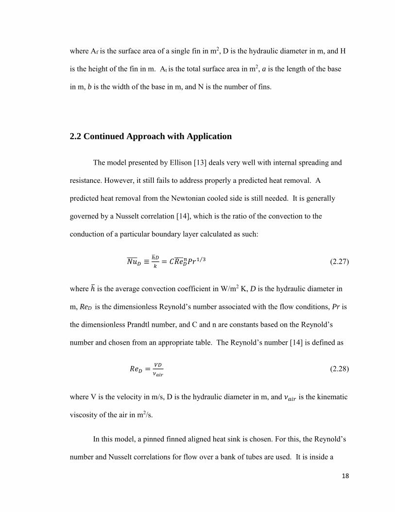
Figure 2.3 Thermal resistance varied against the thermal conductivity while h is held

constant at 150 W/m^2 K

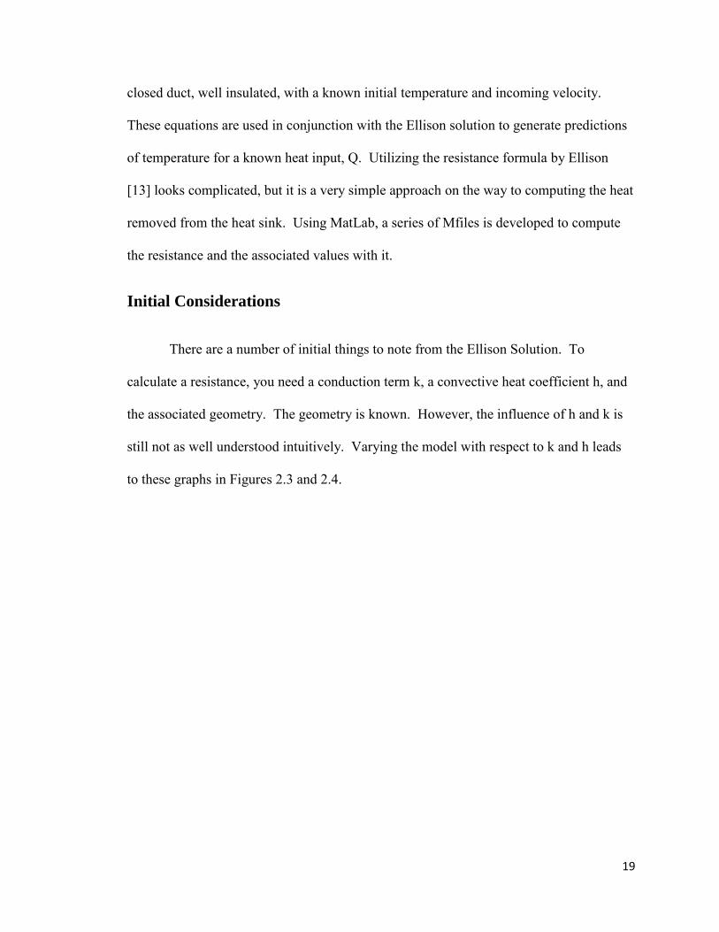
Figure 2.4 Convection coefficient h varied while holding k constant at 1000 W/m K.

0 500 1000 1500 2000 2500 3000 3500 4000 4500 50000.48

0.5

0.52

0.54

0.56

0.58

0.6

Estimated Thermal Conductivity k in W/m K

Therm

al R

esis

tance in K

/W

Variance of Thermal Resistance against Thermal Conductivity k

100 110 120 130 140 150 160 170 180 190 2000.4

0.45

0.5

0.55

0.6

0.65

0.7

0.75

0.8

Convection Coefficient h in W/m2 K

Therm

al R

esis

tance in K

/W

Variance of Thermal Resistance against Convection Coefficent h

21

Figure 2.3 is varied for k values ranging from a value of 400 W/m K to 5,000

W/m K, which is on the lower end of reported effective k values for oscillating heat

pipes. After 2000 to 2500 W/m K, it is noticed that the thermal resistance rapidly

approaches 0.5 K/W. Similarly, in Figure 2.4, k is held constant, that h is varied only

over a value of 100 to 200 W/m2 K and dropping noticeably lower than 0.5 K/W while

over a shorter range. As expected, h is the value that needs to be addressed and all

attempts to remove heat are more dependent upon external flow conditions. The thermal

conductivity k is now assumed to be 2500 W/m K

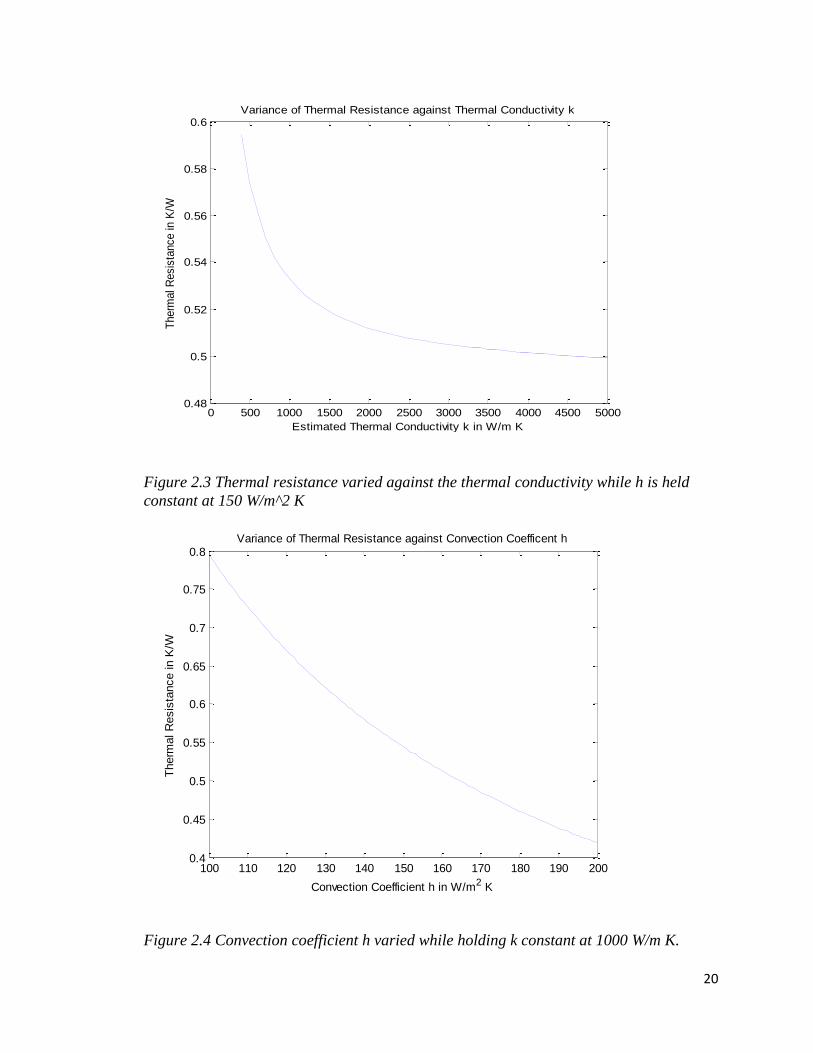
Figure 2.5. Initial computed results plotted. Predictions indicate reasonable values of

surface temperature T.

22

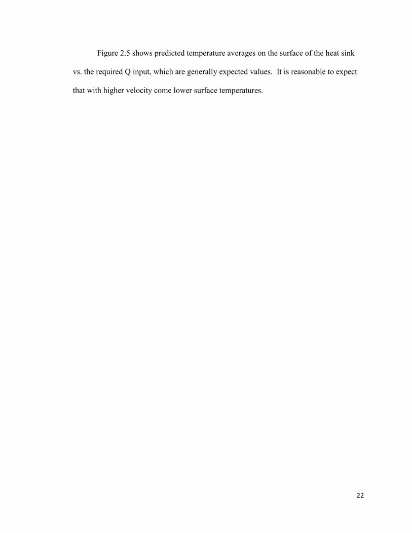
Figure 2.5 shows predicted temperature averages on the surface of the heat sink

vs. the required Q input, which are generally expected values. It is reasonable to expect

that with higher velocity come lower surface temperatures.

23

Chapter 3

Experimental Setup and Procedure

3.1 Experimental Setup

The motivation for this investigation is to determine the use of a flat-plate

oscillating heat pipe (FPOHP) as a thermal spreader. The design of the FPOHP is the

starting point for the experimental setup. Based on the literature review, a similar

previous experimental setup [11], and available stock components, a size of 6.14 in (156

mm) long by 4.1 in (104.1 mm) wide is chosen. It is machined out of a copper plate 0.25

in (6.35 mm) thick. High performance liquid chromatography (HPLC) grade acetone is

chosen as the working fluid. The Bond number governs the maximum diameter of a

working fluid’s ability to form the critical meniscus. The maximum diameter of the

channel for the working fluid can be calculated from

𝐷𝑚𝑎𝑥 = √𝐵𝑜𝑐𝑟𝑖𝑡𝜎

𝑔(𝜌𝑙𝑖𝑞−𝜌𝑣𝑎𝑝) (3.1)

where Bocrit is the critical Bond number, σ is the surface tension in N/m, g is the

acceleration of gravity in m/s2, ρliq is the density of the liquid in kg/m3, and ρvap is the

density of the vapor in kg/m3. A critical Bond number of 1.84 is acknowledged and 1

mm x 1 mm rectangular channels are chosen.

A large number of turns are desirable. For this dimension and design, 34 turns

are implemented. There are 2 mm edges all around to ensure proper brazing area. There

are 2 fill ports of 0.065 in (1.651 mm) in diameter drilled in to meet the channel at both

24

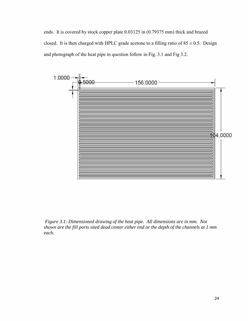
ends. It is covered by stock copper plate 0.03125 in (0.79375 mm) thick and brazed

closed. It is then charged with HPLC grade acetone to a filling ratio of 85 ± 0.5. Design

and photograph of the heat pipe in question follow in Fig. 3.1 and Fig 3.2.

Figure 3.1: Dimensioned drawing of the heat pipe. All dimensions are in mm. Not

shown are the fill ports sited dead center either end or the depth of the channels at 1 mm

each.

25

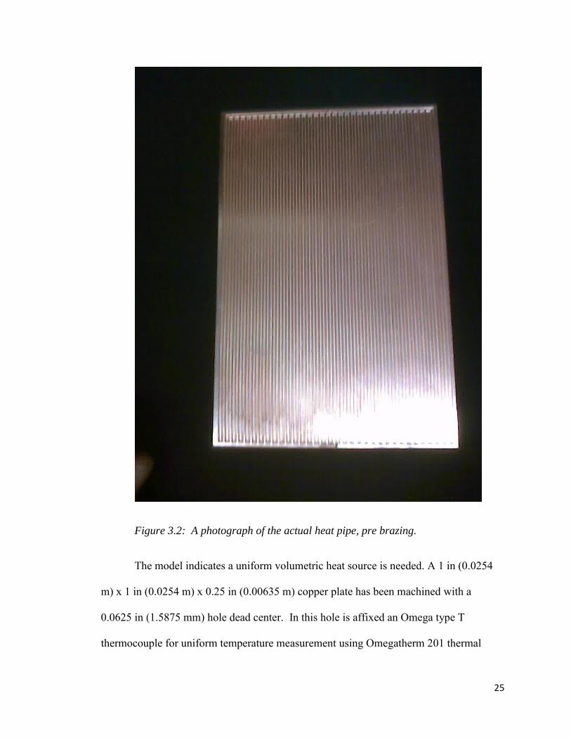
Figure 3.2: A photograph of the actual heat pipe, pre brazing.

The model indicates a uniform volumetric heat source is needed. A 1 in (0.0254

m) x 1 in (0.0254 m) x 0.25 in (0.00635 m) copper plate has been machined with a

0.0625 in (1.5875 mm) hole dead center. In this hole is affixed an Omega type T

thermocouple for uniform temperature measurement using Omegatherm 201 thermal

26

epoxy. Affixed to this are four 250 Watt/10 Ω chip resistors in series from Barry

Industries. These are attached via 2 clamps directly below and in the center of the

FPOHP.

A stock copper heat sink, model number 4-614111U from Cool Innovations is

chosen. It is 4.1 in (0.1041 m) in width by 6.14 in (0.156 m) in length by 1.1 in (0.0279

m) in height. It has 1350 copper pins and has a reported thermal resistance from between

0.14 to 0.07 °C/W depending on the air speed ranging from 1 to 3 m/s. It agrees well

with a calculated thermal resistance from [14] for a pin fin aligned array. It is affixed via

thermal paste (OmegaTherm 201) and held in place with high temp padded insulation and

gently but firmly clamped.

From Interstate Plastics, acrylic polycarbonate (Lexan) sheets are obtained and

joined for the specified dimensions of the wind pipe and heat sink assembly. The wind

tunnel is 4.1 in (0.1041 m) in width by 1.5 in (0.0381 m) in height by 6 ft (1.8 m) long. It

is joined to the inlet of a blower (KoolTronic, Inc Model K37HXFF rated for 3400 RPM)

and tested at velocities of 1 m/s, 2 m/s, and 3 m/s. The blower is powered by a VARIAC

Transformer (Model Number: JPGC-2KM. Input 110V AC 60 Hz) with manually

controlled input.

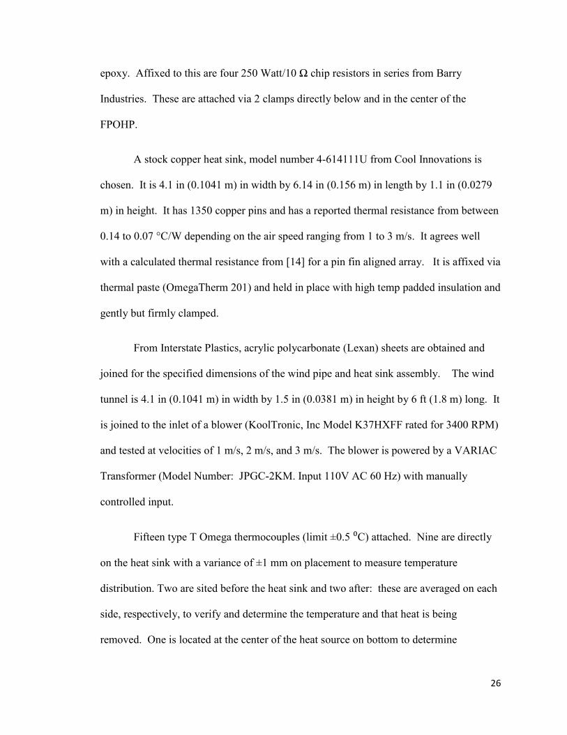
Fifteen type T Omega thermocouples (limit ±0.5 ⁰C) attached. Nine are directly

on the heat sink with a variance of ±1 mm on placement to measure temperature

distribution. Two are sited before the heat sink and two after: these are averaged on each

side, respectively, to verify and determine the temperature and that heat is being

removed. One is located at the center of the heat source on bottom to determine

27

maximum temperature for calculation. One is also placed directly on top of a chip resistor

(Barry Industries 250W/ 10Ω chip resistor) to maintain avoidance of unintentional

burnout, defined as 100⁰C. The layout for the Omega type T thermocouples on the

surface of the heat sink is shown in Fig. 3.3.

The heater is powered by a DC power supply (Agilent Technologies, Model

N5771A. 300V/5A or 1500 Watts). The resistance of the chip resistors and DC power

supply are verified to 39.8 Ω using a handheld digital multi-meter (Fluke 175 True RMS

DMM). The air duct is well sealed with aluminum heater tape (around all edges of the

heat pipe assembly) to prevent air leakage and the heat loss associated with it, only

allowing air movement through both the entrance and exit of the duct. All exterior

surfaces with thermocouples and heat source are well insulated using fiberglass

Topside view of thermocouple array and flow

pattern. Dashed line indicates heat source

and evaporator

Figure 3.3 Topside view of setup showing flow pattern and thermocouple

array

28

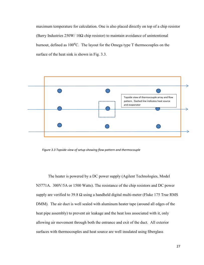
insulation. Design is as depicted in Figures 3.3 and 3.4. These are connected to a DAQ

(National Instruments NI-SCXI-1000) and PC setup (Dell Inspiron 1720 with Windows 7

and Labview Signal Express software package).

Figure 3.5 Block diagram of experimental setup.

29

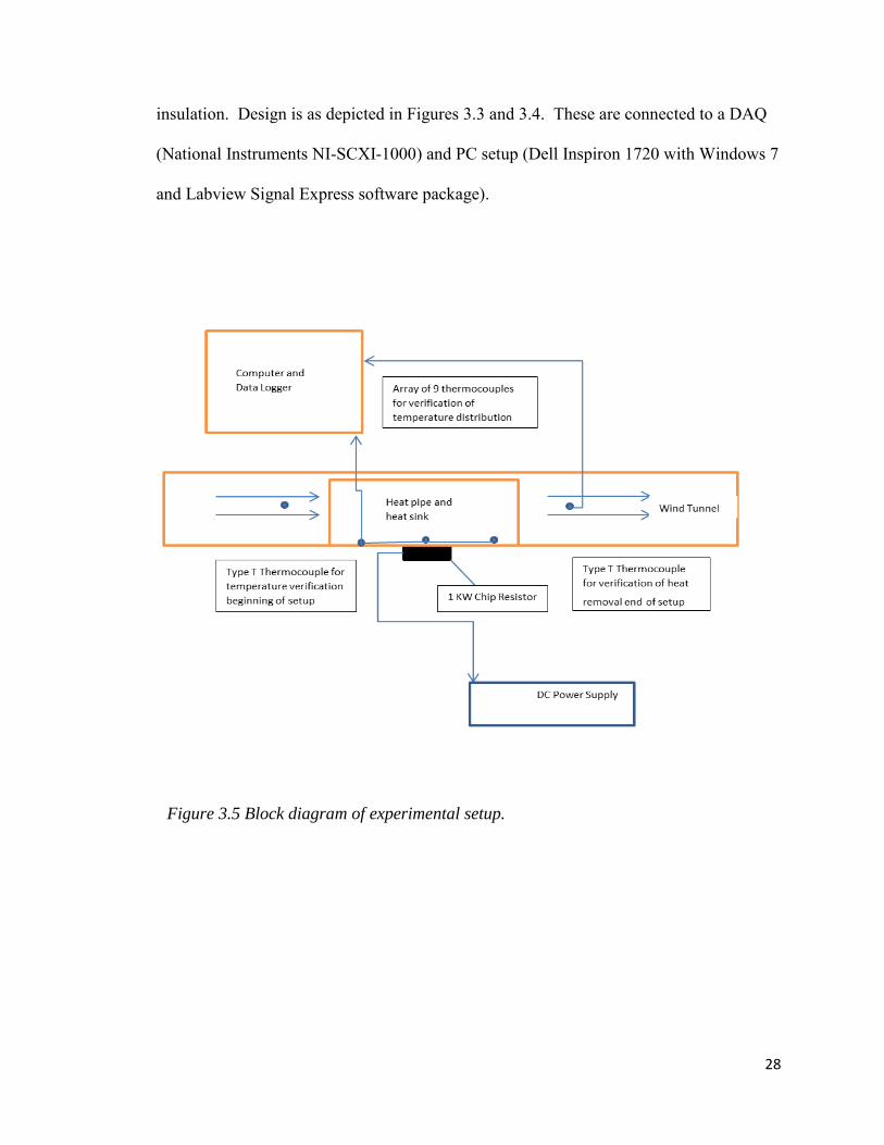
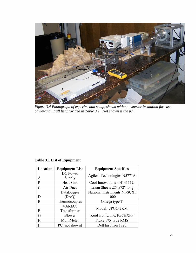
Figure 3.4 Photograph of experimental setup, shown without exterior insulation for ease

of viewing. Full list provided in Table 3.1. Not shown is the pc.

Table 3.1 List of Equipment

Location Equipment List Equipment Specifics

A DC Power

Supply Agilent Technologies N5771A

B Heat Sink Cool Innovations 4-414111U C Air Duct Lexan Sheets .25"x72" long

D DataLogger

(DAQ) National Instruments NI-SCXI

1000 E Thermocouples Omega type T

F VARIAC

Transformer Model: JPGC-2KM

G Blower KoolTronic, Inc. K37HXFF H MultiMeter Fluke 175 True RMS I PC (not shown) Dell Inspiron 1720

30

3.2 Procedure

The assembly is tested at velocities of intervals of 1 m/s from 1 m/s to 3 m/s as

calculated from

𝑄 = 𝑎𝑖𝑟𝑐𝑝,𝑎𝑖𝑟∆𝑇 (3.2)

𝑎𝑖𝑟 = 𝜌𝑎𝑖𝑟𝐴𝑐𝑟𝑜𝑠𝑠𝑉∞ (3.3)

𝑄 = 𝐽𝐼 (3.4)

where Q is the heat input in watts, 𝑎𝑖𝑟 is the mass flow rate of the air in kg/s, ∆𝑇 is the

change in temperature in °C, 𝜌𝑎𝑖𝑟is the density of the air in kg/m3 , 𝐴𝑐𝑟𝑜𝑠𝑠 is the cross

sectional area of the duct in m2 , 𝑉∞ is the average incoming air velocity in m/s, J is the

input voltage in volts, and I is the input current in amperes. For the first input, a minimal

heat input of 10 watts was used to provide a temperature difference to calculate the

velocity. The velocity was manually adjusted by adjusting the input power on the

VARIAC transformer power source for the blower until the needed temperature

difference was reached. The type T thermocouples before and after the heat sink and heat

pipe assembly were averaged for values to verify incoming and exit temperatures. At

these velocities, the heat input is varied in increments of 25 Watts from 25 Watts to a

maximum of 225 Watts. For each increase in heat input, a quasi-steady state was

reached. This took 10 to 15 minutes for each increase in heat input. Temperatures were

recorded for later analysis.

The type T thermocouples on top of the heat sink were used to verify the

temperature distribution and to verify thermal spreading. They were then averaged to

determine an average temperature for the model’s top surface. The thermocouples on the

31

bottom (with the chip resistor setup) are used to verify the temperature of the heat source

and to determine a maximum temperature for later calculation and plotting.

3.3 Uncertainty Analysis

There is a certain measurement uncertainty that will be established for each of the

measured and calculated variables. A textbook, Mechanical Measurements 5th .ed

Chapter 3 [15] provides a straightforward procedure for calculating the propagation of

uncertainty. For uncertainties in independent variables and assuming a linear function y

of several independent variables xi with standard deviation zi, there is a statistical

theorem that integrates them all together for the standard deviation zy such that

𝑧𝑦 = √(𝜕𝑦

𝜕𝑥1 𝑧1)

2

+ (𝜕𝑦

𝜕𝑥2𝑧2)

2

+⋯+ (𝜕𝑦

𝜕𝑥𝑛𝑧𝑛)

2

(3.5)

Similarly, a calculated result in a function is likewise a series of independent variables

with uncertainties ui. To estimate a function’s uncertainty, it is assumed that the

uncertainties are small enough that a first order Taylor series expansion provides a good

approximation such that

𝑢𝑦 = √(𝜕𝑦

𝜕𝑥1 𝑢1)

2

+ (𝜕𝑦

𝜕𝑥2𝑢2)

2

+⋯+ (𝜕𝑦

𝜕𝑥𝑛𝑢𝑛)

2

(3.6)

This approximation will hold true for either bias, By, or precision, Wy, uncertainties.

Since the uncertainties propagate separately, they are combined in a root mean square

method such that

𝑈𝑦 = √𝑃𝑦2 +𝑊𝑦2 (3.7)

32

Following the logic of [15], a procedure is established for calculating the uncertainties

inherent. The initial equations and results will be presented here. However, there are

many derivatives and some, if not most, are excessive for the purposes of this discussion.

All are presented in Appendix C for those who wish the full series of equations.

Combining equations 3.2, 3.3, and 3.4 and solving for V

𝑉 =𝐽𝐼

𝐴𝑐𝑟𝑜𝑠𝑠𝑐𝑝,𝑎𝑖𝑟𝜌𝑎𝑖𝑟∆𝑇 (3.8)

Calculating the derivatives for J, I, Across, and ΔT and using equations 3.6, it is found that

V has a precision uncertainty of 0.002 m/s and a bias uncertainty of 1.5 m/s. Combining

equations 2.27 and 2.28 and solving for h,

ℎ =𝑘

𝐷𝐶𝑃𝑟1/3 (

𝑉𝐷

𝜈𝑎𝑖𝑟)𝑛

(3.9)

Calculating the derivatives for D, V, and νair and using equations 3.6, it is found that h

has a precision uncertainty of 0.31, 0.42, and 0.50 Watts/m2 K and a bias uncertainty of

59.5, 41.1, and 33.1 Watts/m2 K for velocities V of 1, 2, and 3 m/s, respectively.

Combining equations 2.22, 2.23, 2.24, 2.25, and 2.26 and solving for heff

ℎ𝑒𝑓𝑓 =ℎ

4𝑎𝑏(4𝑎𝑏 − 𝐷2𝑁𝜋 −

2𝐷𝑁𝜋 𝑇𝑎𝑛ℎ(2𝐻√ℎ

𝐷𝑘)

√ℎ

𝐷𝑘

) (3.10)

Calculating derivatives for h, a, b, D, and H and using equations 3.6, it is found that heff

has a precision uncertainty of 39.2, 49.7, and 56.3 Watts/m2 K with a bias uncertainty of

638.7, 419.5, and 327.3 Watts/m2 K. Combining equations 2.18, 2.19, 2.20, and 2.21

and reintroducing all dimensioned variables, R is found such that

33

𝑅 =1

√𝑏3𝑎(𝑡

𝑘+

1

ℎ𝑒𝑓𝑓) +

√𝑎3

𝑏3

𝑘∆𝑥𝜋2∑

1

𝑙2𝑆𝑖𝑛 (

𝑙𝜋∆𝑥

𝑎) (

1+ℎ𝑒𝑓𝑓𝑎

2𝑙𝜋𝑘𝑇𝑎𝑛ℎ(

2𝑙𝜋𝑡

𝑎)

ℎ𝑒𝑓𝑓𝑎

2𝑙𝜋𝑘+𝑇𝑎𝑛ℎ(

2𝑙𝜋𝑡

𝑎))1000

𝑙=1 +

√𝑏3

𝑎3

𝑘∆𝑦𝜋2∑

1

𝑚21000𝑚=1 𝑆𝑖𝑛 (

𝑚𝜋𝑎∆𝑦

𝑏2) (

1+ℎ𝑒𝑓𝑓

2𝑘𝑚𝜋𝑇𝑎𝑛ℎ(

2𝑚𝜋𝑡

𝑏)

ℎ𝑒𝑓𝑓

2𝑘𝑚𝜋+𝑇𝑎𝑛ℎ(

2𝑚𝜋𝑡

𝑏)) +

4√𝑎𝑏

𝑘𝜋2∆𝑥∆𝑦∑ ∑

1

𝑙𝑚

1000𝑚=1 𝑆𝑖𝑛 (

𝑙𝜋∆𝑥

𝑎)1000

𝑙=1 𝑆𝑖𝑛 (𝑚𝜋𝑎∆𝑦

𝑏2)

(

1+

ℎ𝑒𝑓𝑓𝑎

2𝜋𝑘√𝑙2+𝑎2𝑚2

𝑏2

𝑇𝑎𝑛ℎ(2𝜋𝑡

𝑎√𝑙2+

𝑎2𝑚2

𝑏2)

(2𝜋𝑡

𝑎√𝑙2+

𝑎2𝑚2

𝑏2)

(

ℎ𝑒𝑓𝑓𝑎


𝑏2

+𝑇𝑎𝑛ℎ(2𝜋𝑡

𝑎√𝑙2+

𝑎2𝑚2

𝑏2)

)

)

(3.11)

Calculating derivatives for h, a, b, t, Δx, and Δy and using equations 3.6 and 3.7, it is

found that R has a total uncertainty of 0.1, 0.09, and 0.08 K/W for V of 1, 2, and 3 m/s

respectively.

34

Chapter 4

Results and discussion

This model is being corroborated not only with new data, but also with older data.

Data from a previous experiment, Fritz Laun [16], was used initially for verification of

the model’s validity. Data was obtained on a centered heat source with a cooling block

attached. There are two sets of data. The cooling block and heat pipe setup is 10 cm x 10

cm and .031 m thick. For the first set, the heater is 3 cm x 3 cm and for the second it is 4

cm x 4 cm. The first set has a copper plate to encourage thermal spreading whereas the

second set does not. The cooling bath is maintained at 20 ⁰C while the power output is

varied from 250 Watts to 350 Watts. The second set is varied from 550 Watts to 600

Watts. Thermal resistance [9] is experimentally calculated as follows:

𝑅 = 𝑇𝑒−𝑇𝑐

𝑄 (4.1)

Where Q is the heat input in Watts, Te is the evaporator temperature in ⁰C and Tc is the

condenser temperature in ⁰C. For the thermal spreading model used, a heat transfer

coefficient is also needed. This is backed out from experimental data via Newton’s Law

of Cooling [14]:

ℎ =𝑄

𝐴∆𝑇 (4.2)

where h is the heat transfer coefficient in W/m2 K, Q is the heat input in Watts, A is the

area of the heat transfer surface in m2 and ΔT is the temperature difference in ⁰C. Table

1 shows the calculated data. As can be seen, there is excellent agreement between the

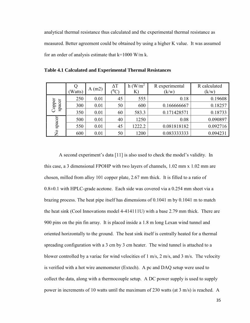
35

analytical thermal resistance thus calculated and the experimental thermal resistance as

measured. Better agreement could be obtained by using a higher K value. It was assumed

for an order of analysis estimate that k=1000 W/m k.

Table 4.1 Calculated and Experimental Thermal Resistances

Q (Watts) A (m2) ΔT

(⁰C) h (W/m2

K) R experimental

(k/w) R calculated

(k/w)

Cop

per

spac

er 250 0.01 45 555 0.18 0.19608

300 0.01 50 600 0.166666667 0.18257 350 0.01 60 583.3 0.171428571 0.18733

No

spac

er

500 0.01 40 1250 0.08 0.090897 550 0.01 45 1222.2 0.081818182 0.092716 600 0.01 50 1200 0.083333333 0.094231

A second experiment’s data [11] is also used to check the model’s validity. In

this case, a 3 dimensional FPOHP with two layers of channels, 1.02 mm x 1.02 mm are

chosen, milled from alloy 101 copper plate, 2.67 mm thick. It is filled to a ratio of

0.8±0.1 with HPLC-grade acetone. Each side was covered via a 0.254 mm sheet via a

brazing process. The heat pipe itself has dimensions of 0.1041 m by 0.1041 m to match

the heat sink (Cool Innovations model 4-414111U) with a base 2.79 mm thick. There are

900 pins on the pin fin array. It is placed inside a 1.8 m long Lexan wind tunnel and

oriented horizontally to the ground. The heat sink itself is centrally heated for a thermal

spreading configuration with a 3 cm by 3 cm heater. The wind tunnel is attached to a

blower controlled by a variac for wind velocities of 1 m/s, 2 m/s, and 3 m/s. The velocity

is verified with a hot wire anemometer (Extech). A pc and DAQ setup were used to

collect the data, along with a thermocouple setup. A DC power supply is used to supply

power in increments of 10 watts until the maximum of 230 watts (at 3 m/s) is reached. A

36

copper plate of nearly identical dimension to the heat pipe is used as a control to verify

experimental performance. T incoming is held constant at 21 ±0.5 °C. Experimental

thermal resistance is calculated from

𝑅 =𝑇𝑚𝑎𝑥−𝑇∞

𝑄 (4.3)

where Tmax is the maximum time-averaged temperature in ⁰C, T∞ is the incoming

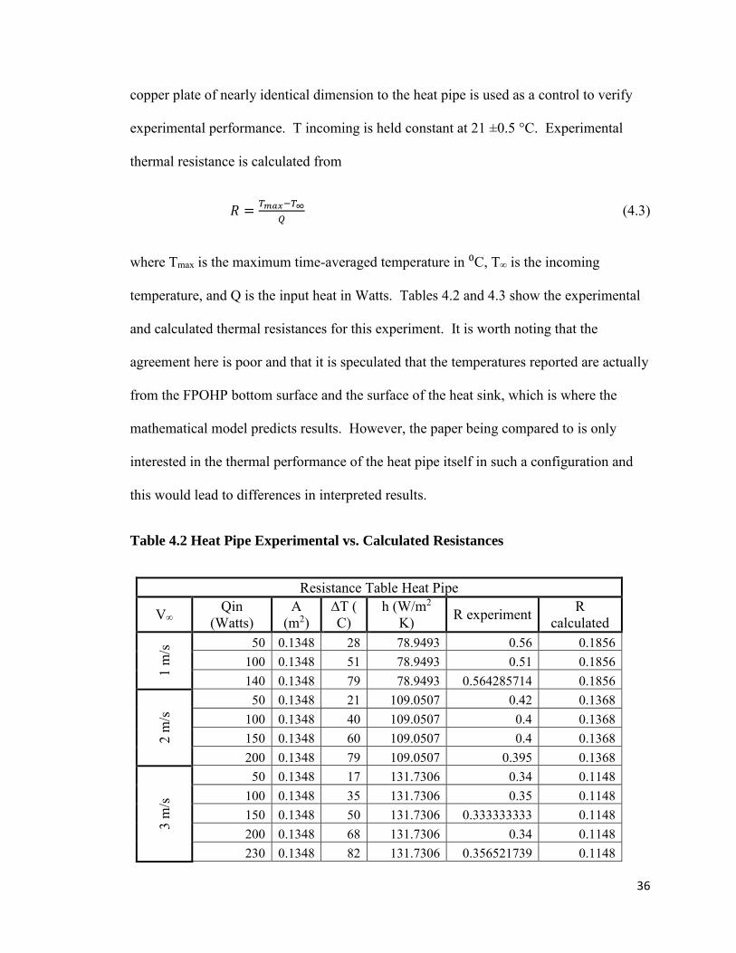
temperature, and Q is the input heat in Watts. Tables 4.2 and 4.3 show the experimental

and calculated thermal resistances for this experiment. It is worth noting that the

agreement here is poor and that it is speculated that the temperatures reported are actually

from the FPOHP bottom surface and the surface of the heat sink, which is where the

mathematical model predicts results. However, the paper being compared to is only

interested in the thermal performance of the heat pipe itself in such a configuration and

this would lead to differences in interpreted results.

Table 4.2 Heat Pipe Experimental vs. Calculated Resistances

Resistance Table Heat Pipe

V∞ Qin (Watts)

A (m2)

∆T ( C)

h (W/m2 K) R experiment R

calculated

1 m

/s 50 0.1348 28 78.9493 0.56 0.1856

100 0.1348 51 78.9493 0.51 0.1856 140 0.1348 79 78.9493 0.564285714 0.1856

2 m

/s 50 0.1348 21 109.0507 0.42 0.1368 100 0.1348 40 109.0507 0.4 0.1368 150 0.1348 60 109.0507 0.4 0.1368 200 0.1348 79 109.0507 0.395 0.1368

3 m

/s

50 0.1348 17 131.7306 0.34 0.1148 100 0.1348 35 131.7306 0.35 0.1148 150 0.1348 50 131.7306 0.333333333 0.1148 200 0.1348 68 131.7306 0.34 0.1148 230 0.1348 82 131.7306 0.356521739 0.1148

37

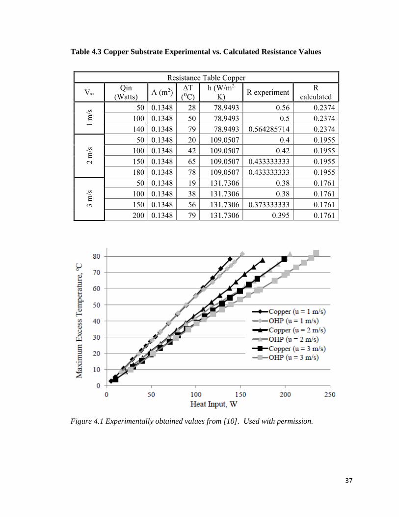
Table 4.3 Copper Substrate Experimental vs. Calculated Resistance Values

Resistance Table Copper

V∞ Qin (Watts) A (m2) ∆T

(⁰C) h (W/m2

K) R experiment R calculated

1 m

/s 50 0.1348 28 78.9493 0.56 0.2374

100 0.1348 50 78.9493 0.5 0.2374 140 0.1348 79 78.9493 0.564285714 0.2374

2 m

/s 50 0.1348 20 109.0507 0.4 0.1955

100 0.1348 42 109.0507 0.42 0.1955 150 0.1348 65 109.0507 0.433333333 0.1955 180 0.1348 78 109.0507 0.433333333 0.1955

3 m

/s 50 0.1348 19 131.7306 0.38 0.1761

100 0.1348 38 131.7306 0.38 0.1761 150 0.1348 56 131.7306 0.373333333 0.1761 200 0.1348 79 131.7306 0.395 0.1761

Figure 4.1 Experimentally obtained values from [10]. Used with permission.

38

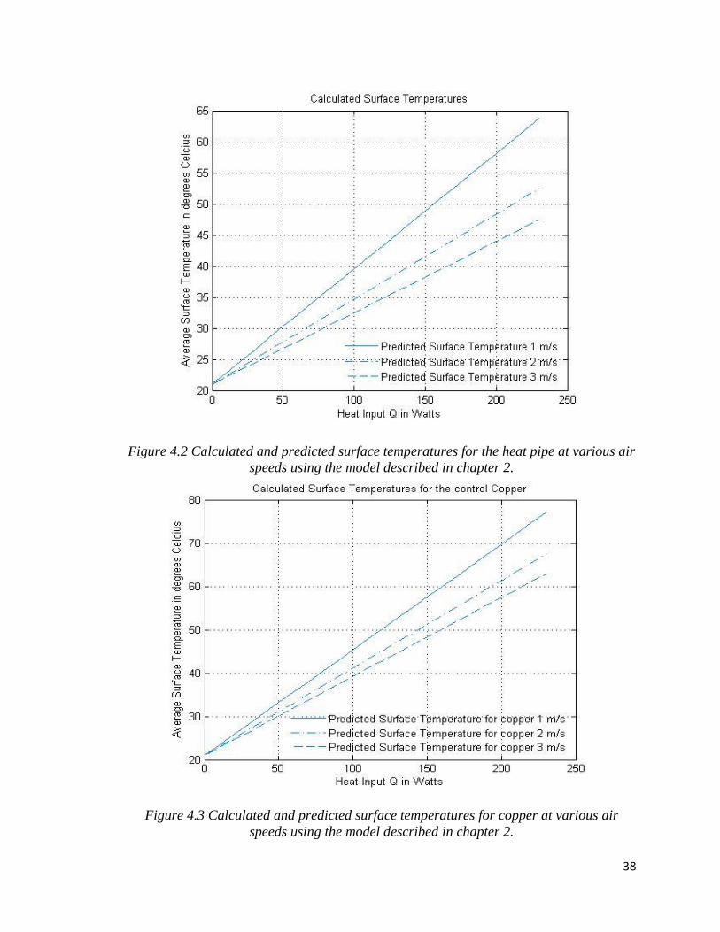
Figure 4.2 Calculated and predicted surface temperatures for the heat pipe at various air

speeds using the model described in chapter 2.

Figure 4.3 Calculated and predicted surface temperatures for copper at various air

speeds using the model described in chapter 2.

39

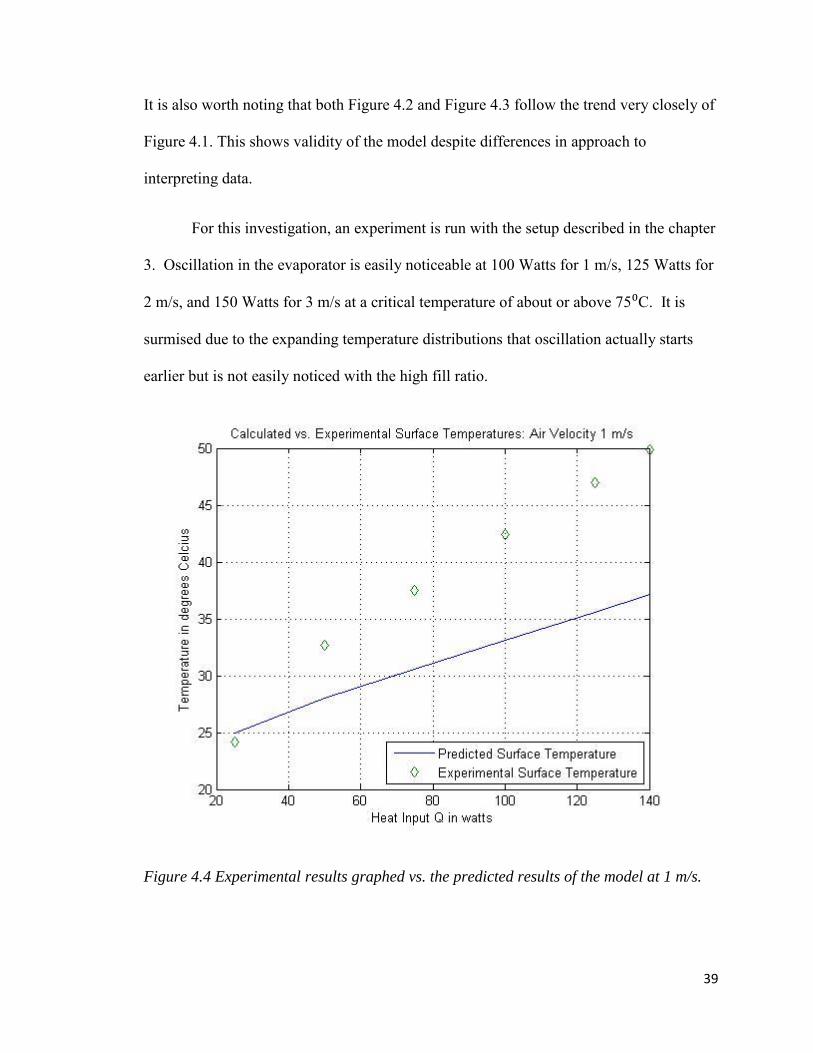
It is also worth noting that both Figure 4.2 and Figure 4.3 follow the trend very closely of

Figure 4.1. This shows validity of the model despite differences in approach to

interpreting data.

For this investigation, an experiment is run with the setup described in the chapter

3. Oscillation in the evaporator is easily noticeable at 100 Watts for 1 m/s, 125 Watts for

2 m/s, and 150 Watts for 3 m/s at a critical temperature of about or above 75⁰C. It is

surmised due to the expanding temperature distributions that oscillation actually starts

earlier but is not easily noticed with the high fill ratio.

Figure 4.4 Experimental results graphed vs. the predicted results of the model at 1 m/s.

40



41

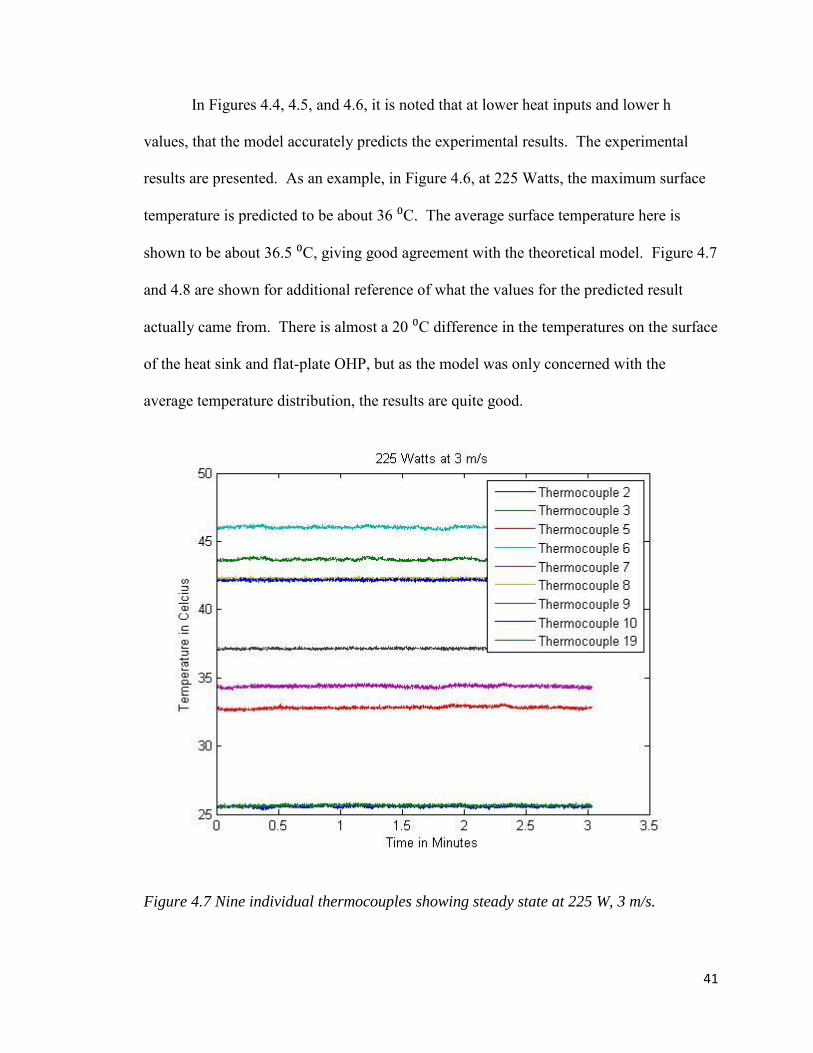
In Figures 4.4, 4.5, and 4.6, it is noted that at lower heat inputs and lower h

values, that the model accurately predicts the experimental results. The experimental

results are presented. As an example, in Figure 4.6, at 225 Watts, the maximum surface

temperature is predicted to be about 36 ⁰C. The average surface temperature here is

shown to be about 36.5 ⁰C, giving good agreement with the theoretical model. Figure 4.7

and 4.8 are shown for additional reference of what the values for the predicted result

actually came from. There is almost a 20 ⁰C difference in the temperatures on the surface

of the heat sink and flat-plate OHP, but as the model was only concerned with the

average temperature distribution, the results are quite good.

Figure 4.7 Nine individual thermocouples showing steady state at 225 W, 3 m/s.

42

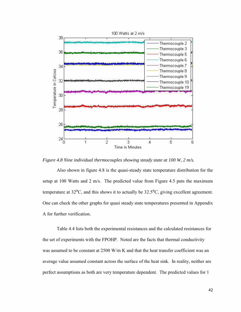
Figure 4.8 Nine individual thermocouples showing steady state at 100 W, 2 m/s.

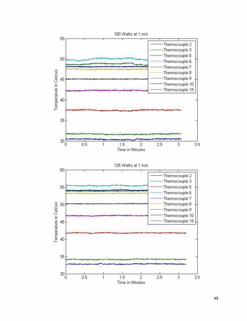
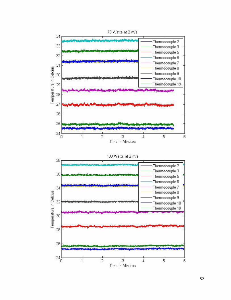
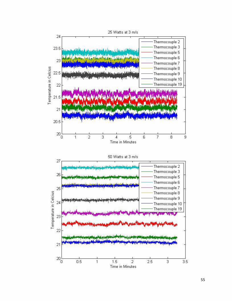
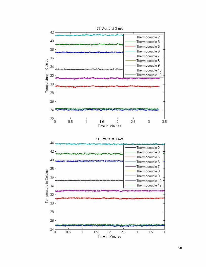
Also shown in figure 4.8 is the quasi-steady state temperature distribution for the

setup at 100 Watts and 2 m/s. The predicted value from Figure 4.5 puts the maximum

temperature at 32⁰C, and this shows it to actually be 32.5⁰C, giving excellent agreement.

One can check the other graphs for quasi steady state temperatures presented in Appendix

A for further verification.

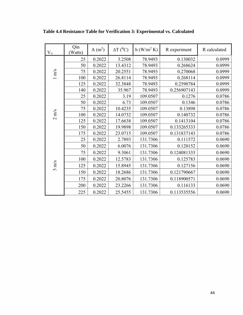
Table 4.4 lists both the experimental resistances and the calculated resistances for

the set of experiments with the FPOHP. Noted are the facts that thermal conductivity

was assumed to be constant at 2500 W/m K and that the heat transfer coefficient was an

average value assumed constant across the surface of the heat sink. In reality, neither are

perfect assumptions as both are very temperature dependent. The predicted values for 1

43

m/s were mostly off by a fair margin. However, when it starts oscillating at around 100

Watts, the resistances start decreasing, which would be consistent with an increasing

thermal conductivity associated with an oscillating heat pipe. The values predicted for 2

m/s and 3 m/s were actually quite accurate, particularly for such basic steady state

assumptions. It is noted that the h value associated with 1 m/s is high for a transitional

flow region and as such, under predicts the actual results considerably. The theoretical h-

value is definitely too high but still gives reasonably good results. The value of h

associated with 2 and 3 m/s flows is predicted quite well for turbulent flow regions and

gives good results. The calculated R values are calculated from equation 4.3, which is

only concerned with the maximum time averaged surface temperature.

44

Table 4.4 Resistance Table for Verification 3: Experimental vs. Calculated

V∞ Qin

(Watts) A (m2) ∆T (⁰C) h (W/m2 K) R experiment R calculated 1

m/s

25 0.2022 3.2508 78.9493 0.130032 0.0999 50 0.2022 13.4312 78.9493 0.268624 0.0999 75 0.2022 20.2551 78.9493 0.270068 0.0999

100 0.2022 26.8114 78.9493 0.268114 0.0999 125 0.2022 32.3848 78.9493 0.2590784 0.0999 140 0.2022 35.967 78.9493 0.256907143 0.0999

2 m

/s

25 0.2022 3.19 109.0507 0.1276 0.0786 50 0.2022 6.73 109.0507 0.1346 0.0786 75 0.2022 10.4235 109.0507 0.13898 0.0786

100 0.2022 14.0732 109.0507 0.140732 0.0786 125 0.2022 17.6638 109.0507 0.1413104 0.0786 150 0.2022 19.9898 109.0507 0.133265333 0.0786 175 0.2022 23.0715 109.0507 0.131837143 0.0786

3 m

/s

25 0.2022 2.7893 131.7306 0.111572 0.0690 50 0.2022 6.0076 131.7306 0.120152 0.0690 75 0.2022 9.3061 131.7306 0.124081333 0.0690

100 0.2022 12.5783 131.7306 0.125783 0.0690 125 0.2022 15.8945 131.7306 0.127156 0.0690 150 0.2022 18.2686 131.7306 0.121790667 0.0690 175 0.2022 20.8076 131.7306 0.118900571 0.0690 200 0.2022 23.2266 131.7306 0.116133 0.0690 225 0.2022 25.5455 131.7306 0.113535556 0.0690

45

Chapter 5

Conclusions

A literature review on thermal spreading and mathematical models has been done.

Many had useful information regarding the operation of oscillating heat pipes but were

primarily axial configurations. Only one concerned itself with a thermal spreading

configuration. Using an analytical approach similar to calculating the spreading

resistance presented in one of the reviewed papers [13], three sets of data were analyzed.

Two were existing experiments, and the third was one made for the purpose of testing

this model. One experiment was a 3D FPOHP design in a square configuration with

similar setup to the one presented in this paper. It did not give good agreement with the

model, though the other two did. It should be noted that for this experiment the predicted

values of the maximum surface temperature were plotted, and while they were lower than

the reported values, there was generally excellent and what appeared to be direct linear

agreement with the trends and data presented. An experiment was conducted to verify

the values of the model in a bottom centered heating thermal spreading configuration at

various velocities. The results were reported and there is generally good agreement with

the thermal resistance model presented. The model accurately calculates a spreading

resistance. Measured resistance doesn’t necessarily correspond to calculated spreading

resistances. It does, however, relatively accurately predict the average surface

temperature of the heat sink and flat plate oscillating heat pipe combination, which again

points to the validity of the model presented.

46

References

1. Akachi, H., 1990, “Structure of a Heat Pipe,” U.S. Patent 4,921,041. 2. Khandekar, S., Schneider M.,Schafer, R., Kulenovic R., Groll, M., 2002,

“Thermofluid Dynamic Study of Flat-Plate Closed-Loop Pulsating Heat Pipes,” Microscale Thermophysical Engineering. Vol.6, pp. 303-317.

3. Charoensawan, P., Khandekar. S., Groll, M., Terdtoon, P. 2003. “Closed loop pulsating heat pipes Part A: parametric experimental investigations”, Applied Thermal Engineering. Vol.23 . pp. 2009-2020.

4. Chien, K.H, Chen Y.R., Lin Y.T., Wang C.C., Yang K.S. “The Experimental Studies of Flat-Plate Closed-Loop Pulsating Heat Pipes,” International 10th Heat Pipe Symposium, p.p. 212-216.

5. Charoensawan, P., Terdtoon, P., 2007. “Thermal Performance Correlation of Horizontal Closed-Loop Oscillating Heat Pipes,” Electronics Packing Technology Conference, pp. 906-909.

6. Charoensawan, P., Terdtoon, P.,2008, “Thermal performance of horizontal closed-loop oscillating heat pipes,” Applied Thermal Engineering, Vol. 8, pp. 460-466.

7. Ma, H., Cheng, P., 2011,”A Mathematical Model of an Oscillating Heat Pipe,” Heat Transfer Engineering, Vol.32:11-12, pp. 1037-1046.

8. Chen, J.C., 1966, “Correlation for Boiling Heat Transfer to Saturated Fluids in Convective Flow,” Ind. Eng. Chem. Process Des. Dev., 5_3_,pp. 322-339.

9. Khandekar, S., Charoensawan, P.,Groll, M., Terdtoon,P., 2003, “Closed loop pulsating heat pipes Part B: visualization and semi-empirical modeling”, 18th National and 7th ISHMT-ASME Heat and Mass Transfer Conference, p.p. 1-12.

10. Khandekar, S., Groll, M. 2008, “Roadmap to Realistic Modeling of Closed Loop Pulsating Heat Pipes”, 9th International Heat Pipe Symposium, p.p. 1-12.

11. Thompson, S.M., Ma, Lu, H., Ma, H. B., 2013, “Experimental Investigation of Flat-Plate Oscillating Heat Pipe for Thermal Spreading Application,” 51st AIAA Aerospace Sciences Meeting including the New Horizons Forum and Aerospace Exposition, Paper No. AIAA 2013-0309, Grapevine, TX, USA|| DOI:10.2514/6.2013-309.

12. Zhang, Y.,Faghri, A., 2008,”Advances and Unsolved Issues in Pulsating Heat Pipes,” Heat Transfer Engineering, Vol. 29:1,pp.20-44.

13. Ellison, G. 2003,”Maximum Thermal Spreading Resistance for Rectangular Sources and Plates with Non-unity Aspect Ratios,” IEEE Transactions on Components and Packaging Technologies, Vol. 26:2, pp. 439-454.

14. Incropera, F. P., DeWitt, D. P., 2002, Introduction to Heat Transfer, 4th

ed., John Wiley & Sons, New York.

15. Beckwith, T. G., Marangoni, R.D, Lienhard, J.H., 1995, Mechanical Measurements, 5th ed., Addison Wesley Publishing Company, Massachussets

16. Laun, Fritz.,2013, “Experimental Investigation of Oscillating Heat Pipes,” Masters thesis, University of Missouri, Columbia Missouri

47

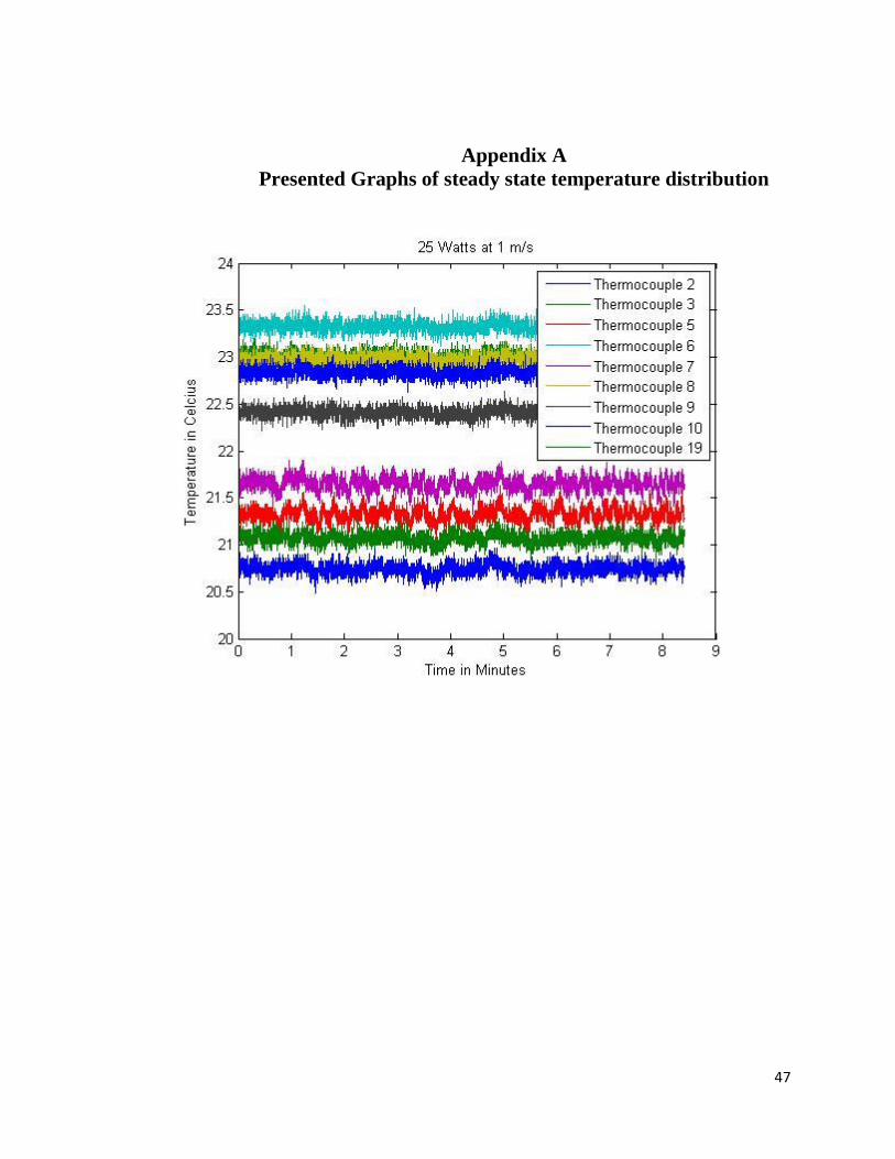
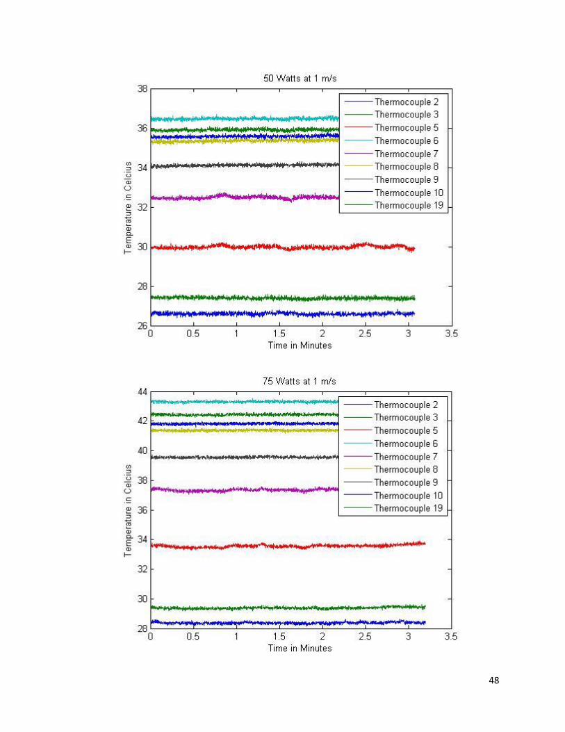
Appendix A

Presented Graphs of steady state temperature distribution

60

Appendix B

Matlab Code used for Calculation

Resist.m: Used to calculate resistance and spreading resist for all cases

function spread=resist(deltax,deltay,a,b,t,h,k) % deltax=length of heat source in meters % deltay=width of heat source in meters % a=length of heat sink in meters % b=width of heat sink in meters % t=thickness of thermal spreader in meters % h=heat transfer coefficient off of heat sink in Watts/meter squared % Kelvin alpha=deltax/a; beta=deltay/b; ro=a/b; tau=t/a; Biottau=h*t/k; psiu=ro*tau*sqrt(alpha*beta)*(1+1/Biottau); y=zeros(1,300); for i=1:300 y(i)=(ro/pi^2)*sqrt(beta/alpha)*(1/i^2)*sin(i*pi*alpha)*((1+((Biottau/(2*pi*tau*i))*tanh(2*i*pi*tau)))/((Biottau/(2*pi*tau*i))+tanh(2*i*pi*tau))); end x=zeros(1,300); for j=1:300 x(j)=(1/(ro*pi^2))*sqrt(alpha/beta)*(1/j^2)*sin(j*pi*beta*ro)*((1+((Biottau/(2*j*pi*ro*tau))*tanh(2*j*pi*ro*tau)))/((Biottau/(2*j*pi*ro*tau))+tanh(2*j*pi*ro*tau))); end xy=zeros(300,300); for L=1:300 for m=1:300 xy(L,m)=(4/(pi^2*sqrt(alpha*beta)))*1/(L*m)*sin(L*pi*alpha)*sin(m*pi*beta*ro)*(1+((Biottau/(2*pi*tau*sqrt(L^2+m^2*ro^2)))*tanh(2*pi*tau*sqrt(L^2+m^2*ro^2))))/((2*pi*sqrt(L^2+m^2*ro^2)*((Biottau/(2*pi*tau*sqrt(L^2+m^2*ro^2)))+tanh(2*pi*tau*sqrt(L^2+m^2*ro^2))))); end end psispread=sum(y)+sum(x)+sum(sum(xy)); spread=psispread/(k*sqrt(deltax*deltay))+psiu/(k*sqrt(deltax*deltay));

61

CallResist.m: Matlab code used to calculate and plot theoretical values for a given

geometry

for j=0:100:5000 j=j+400; k(j)=resist(.0254,.0254,.156,.1041,.006,153.6,j); end % knew=k(400:100:5000); % % plot(linspace(400,5000,length(knew)),knew) % xlabel('Estimated Thermal Conductivity k in W/m K') % ylabel('Thermal Resistance in K/W') % title('Variance of Thermal Resistance against Thermal Conductivity k') % Resistances varied according to show dependance of thermal resistance % upon h for i=100:200 h(i)=resist(.0254,.0254,.156,.1041,.006,i,1000); end plot(linspace(100,length(h),101),h(100:200));

62

CallResist2: Matlab code used to calculate and plot values for experimental data.

uinf1=1;uinf2=2;uinf3=3;%m/s Dh=.001778; %m mu=16.505*10^-6; %m^2/s Pr=0.712; k=0.026; %W/m^2 K Nf=1350;%number of fins in array L=0.156;%length of heat sink in meters W=0.1041;%width of heat sink in meters hfin=0.025146;%height of fin in meters kcu=401; %W/m K %calculate reynold's number approximating as a single isolated cylinder ReL1=uinf1*Dh/mu; ReL2=uinf2*Dh/mu; ReL3=uinf3*Dh/mu; %calculate nusselt number based on Reynold's number Nu1=.683*ReL1^(.466)*Pr^(1/3); Nu2=.683*ReL2^(.466)*Pr^(1/3); Nu3=.683*ReL3^(.466)*Pr^(1/3); %calculate average heat transfer coefficient h1=Nu1*k/Dh; h2=Nu2*k/Dh; h3=Nu3*k/Dh; % calculate m and from that, fin efficiency based on h value m1=((4*h1)/(kcu*Dh))^0.5; m2=((4*h2)/(kcu*Dh))^0.5; m3=((4*h3)/(kcu*Dh))^0.5; fineff1=tanh(m1*(hfin+Dh/4))/(m1*(hfin+Dh/4)); fineff2=tanh(m2*(hfin+Dh/4))/(m2*(hfin+Dh/4)); fineff3=tanh(m3*(hfin+Dh/4))/(m3*(hfin+Dh/4)); %Af and At, specifically the Area of the fin and the total surface area in %square meters Af=pi*Dh*hfin; At=Nf*Af+L*W-Nf*pi*(Dh/2)^2; %account for extra area of heat sink in a ratio and calculate heff. done by means of comparing heff to true h with fins. h1eff=h1*At*(1-(Nf*Af*(1-fineff1)/At))/(L*W); h2eff=h2*At*(1-(Nf*Af*(1-fineff2)/At))/(L*W); h3eff=h3*At*(1-(Nf*Af*(1-fineff3)/At))/(L*W); psi1=resist(.0254,.0254,.156,.1041,.006,h1eff,2500) psi2=resist(.0254,.0254,.156,.1041,.006,h2eff,2500) psi3=resist(.0254,.0254,.156,.1041,.006,h3eff,2500)

63

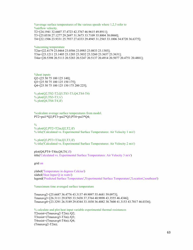
%average surface temperatures of the various speeds where 1,2,3 refer to %airflow velocity. T2=[24.1941 32.6607 37.4723 42.3767 46.9615 49.8911]; T3=[25.0538 27.1277 29.2697 31.5673 33.7109 35.8004 38.0060]; T4=[22.1506 23.9331 25.7937 27.6333 29.4945 31.2565 33.1006 34.8720 36.6375]; %incoming temperature T2in=[22.4179 23.0464 23.0586 23.0983 23.0833 23.1303]; T3in=[23.1211 23.1405 23.1203 23.3032 23.3260 23.3657 23.3631]; T4in=[20.5398 20.5113 20.5283 20.5247 20.5137 20.4914 20.5077 20.4751 20.4881]; %heat inputs Q2=[25 50 75 100 125 140]; Q3=[25 50 75 100 125 150 175]; Q4=[25 50 75 100 125 150 175 200 225]; % plot(Q2,TS2-T2,Q3,TS3-T3,Q4,TS4-T4) % plot(Q3,TS3-T3,'x') % plot(Q4,TS4-T4,'d') %calculate average surface temperatures from model. PT2=psi1*Q2;PT3=psi2*Q3;PT4=psi3*Q4; % % plot(Q2,PT2+T2in,Q2,T2,'d') % title('Calculated vs. Experimental Surface Temperatures: Air Velocity 1 m/s') % plot(Q3,PT3+T3in,Q3,T3,'d') % title('Calculated vs. Experimental Surface Temperatures: Air Velocity 2 m/s') plot(Q4,PT4+T4in,Q4,T4,'d') title('Calculated vs. Experimental Surface Temperatures: Air Velocity 3 m/s') grid on ylabel('Temperature in degrees Celcius') xlabel('Heat Input Q in watts') legend('Predicted Surface Temperature','Experimental Surface Temperature','Location','southeast') %maximum time averaged surface temperature Tmaxavg2=[25.6687 36.4776 43.3137 49.9097 55.4681 59.0973]; Tmaxavg3=[26.3111 29.8705 33.5438 37.3764 40.9898 43.3555 46.4346]; Tmaxavg4=[23.3291 26.5189 29.8344 33.1030 36.4082 38.7600 41.3153 43.7017 46.0336]; % calculate and plot heat input variable experimental thermal resistances T2resist=(Tmaxavg2-T2in)./Q2; T3resist=(Tmaxavg3-T3in)./Q3; T4resist=(Tmaxavg4-T4in)./Q4; (Tmaxavg2-T2in);

64

(Tmaxavg3-T3in); (Tmaxavg4-T4in); % %Preliminary results. Tinput is assumed to be 25 C % q=25:25:500; % dt1=psi1*q;dt2=psi2*q;dt3=psi3*q; % T=25*ones(1,length(q)); % plot(q,dt1+T,q,dt2+T,q,dt3+T) % % % title('Predicted Average Surface Temperature') % ylabel('Temperature in degrees Celcius') % xlabel('Heat Input Q in watts') % grid on % % legend('Heat Removal Air Velocity 1 m/s','Heat Removal Air Velocity 2 m/s','Heat Removal Air Velocity 3 m/s') % legend boxoff

65

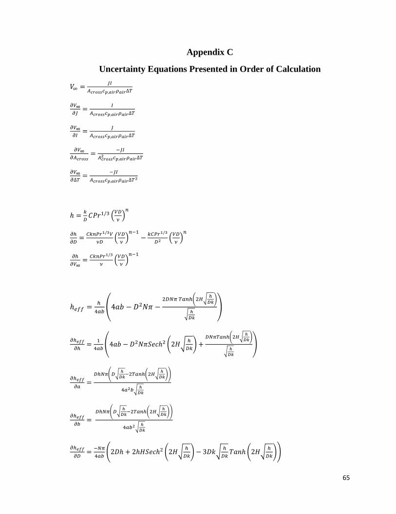
Appendix C

Uncertainty Equations Presented in Order of Calculation

𝑉∞ =𝐽𝐼

𝐴𝑐𝑟𝑜𝑠𝑠𝑐𝑝,𝑎𝑖𝑟𝜌𝑎𝑖𝑟∆𝑇

𝜕𝑉∞

𝜕𝐽=

𝐼


𝜕𝑉∞

𝜕𝐼=

𝐽


𝜕𝑉∞

𝜕𝐴𝑐𝑟𝑜𝑠𝑠=

−𝐽𝐼

𝐴𝑐𝑟𝑜𝑠𝑠2 𝑐𝑝,𝑎𝑖𝑟𝜌𝑎𝑖𝑟∆𝑇

𝜕𝑉∞

𝜕∆𝑇=

−𝐽𝐼

𝐴𝑐𝑟𝑜𝑠𝑠𝑐𝑝,𝑎𝑖𝑟𝜌𝑎𝑖𝑟∆𝑇2

ℎ =𝑘

𝐷𝐶𝑃𝑟1/3 (

𝑉𝐷

𝜈)𝑛

𝜕ℎ

𝜕𝐷=

𝐶𝑘𝑛𝑃𝑟1/3𝑉

𝜈𝐷(𝑉𝐷

𝜈)𝑛−1

−𝑘𝐶𝑃𝑟1/3

𝐷2(𝑉𝐷

𝜈)𝑛

𝜕ℎ

𝜕𝑉∞=

𝐶𝑘𝑛𝑃𝑟1/3

𝜈(𝑉𝐷

𝜈)𝑛−1

ℎ𝑒𝑓𝑓 =ℎ

4𝑎𝑏(4𝑎𝑏 − 𝐷2𝑁𝜋 −

2𝐷𝑁𝜋 𝑇𝑎𝑛ℎ(2𝐻√ℎ

𝐷𝑘)

√ℎ

𝐷𝑘

)

𝜕ℎ𝑒𝑓𝑓

𝜕ℎ=

1

4𝑎𝑏(4𝑎𝑏 − 𝐷2𝑁𝜋𝑆𝑒𝑐ℎ2 (2𝐻√

ℎ

𝐷𝑘) +

𝐷𝑁𝜋𝑇𝑎𝑛ℎ(2𝐻√ℎ

𝐷𝑘)

√ℎ

𝐷𝑘

)

𝜕ℎ𝑒𝑓𝑓

𝜕𝑎=

𝐷ℎ𝑁𝜋(𝐷√ℎ

𝐷𝑘−2𝑇𝑎𝑛ℎ(2𝐻√

ℎ

𝐷𝑘))

4𝑎2𝑏√ℎ

𝐷𝑘

𝜕ℎ𝑒𝑓𝑓

𝜕𝑏=

𝐷ℎ𝑁𝜋(𝐷√ℎ

𝐷𝑘−2𝑇𝑎𝑛ℎ(2𝐻√

ℎ

𝐷𝑘))

4𝑎𝑏2√ℎ

𝐷𝑘

𝜕ℎ𝑒𝑓𝑓

𝜕𝐷=

−𝑁𝜋

4𝑎𝑏(2𝐷ℎ + 2ℎ𝐻𝑆𝑒𝑐ℎ2 (2𝐻√

ℎ

𝐷𝑘) − 3𝐷𝑘√

ℎ

𝐷𝑘𝑇𝑎𝑛ℎ (2𝐻√

ℎ

𝐷𝑘))

66

𝜕ℎ𝑒𝑓𝑓

𝜕𝐻=

𝐷ℎ𝑁𝜋𝑆𝑒𝑐ℎ2(2𝐻√ℎ

𝐷𝑘)

𝑎𝑏

𝑅𝑈 =1

√𝑏3𝑎(𝑡

𝑘+

1

ℎ𝑒𝑓𝑓)

𝜕𝑅𝑈

𝜕𝑎=

−𝑏3

2(𝑎𝑏3)3/2(𝑡

𝑘+

1

ℎ𝑒𝑓𝑓)

𝜕𝑅𝑈

𝜕𝑏=

−3𝑎𝑏2

2(𝑎𝑏3)3/2(𝑡

𝑘+

1

ℎ𝑒𝑓𝑓)

𝜕𝑅𝑈

𝜕𝑡=

1

𝑘√𝑎𝑏3

𝜕𝑅𝑈

𝜕ℎ𝑒𝑓𝑓=

−1

ℎ𝑒𝑓𝑓2 √𝑎𝑏3

𝜕𝑅𝑈

𝜕∆𝑥=

𝜕𝑅𝑈

𝜕∆𝑦= 0

𝑅𝑠𝑝 =√𝑎

3

𝑏3

𝑘∆𝑥𝜋2∑

1

𝑙2𝑆𝑖𝑛 (

𝑙𝜋∆𝑥

𝑎)(

1+ℎ𝑒𝑓𝑓𝑎

2𝑙𝜋𝑘𝑇𝑎𝑛ℎ(

2𝑙𝜋𝑡

𝑎)

ℎ𝑒𝑓𝑓𝑎

2𝑙𝜋𝑘+𝑇𝑎𝑛ℎ(

2𝑙𝜋𝑡

𝑎))1000

𝑙=1 +

√𝑏3

𝑎3

𝑘∆𝑦𝜋2∑

1

𝑚21000𝑚=1 𝑆𝑖𝑛 (

𝑚𝜋𝑎∆𝑦

𝑏2)(

1+ℎ𝑒𝑓𝑓

2𝑘𝑚𝜋𝑇𝑎𝑛ℎ(

2𝑚𝜋𝑡

𝑏)

ℎ𝑒𝑓𝑓


2𝑚𝜋𝑡

𝑏)) +

4√𝑎𝑏


1

𝑙𝑚1000𝑚=1 𝑆𝑖𝑛 (

𝑙𝜋∆𝑥

𝑎)1000

𝑙=1 𝑆𝑖𝑛 (𝑚𝜋𝑎∆𝑦

𝑏2) ∗

(

1+

ℎ𝑒𝑓𝑓𝑎


𝑏2


𝑎√𝑙2+

𝑎2𝑚2

𝑏2)

(2𝜋𝑡

𝑎√𝑙2+

𝑎2𝑚2

𝑏2)

(

ℎ𝑒𝑓𝑓𝑎


𝑏2


𝑎√𝑙2+

𝑎2𝑚2

𝑏2)

)

)

𝜕𝑅𝑠𝑝

𝜕𝑎=

1

𝑘𝜋2∆𝑥∑

3𝑎2

2𝑏3√𝑎3

𝑏3

1000𝑙=1

Sin(𝑙𝜋∆𝑥

𝑎)(1+

𝑎 ℎ𝑒𝑓𝑓 𝑇𝑎𝑛ℎ(2𝑙𝜋𝑡𝑎 )

2𝑘𝑙𝜋)

𝑙2(𝑎ℎ𝑒𝑓𝑓

2𝑘𝑙𝜋+𝑇𝑎𝑛ℎ(

2𝑙𝜋𝑡

𝑎))

+

√𝑎3

𝑏3[Sin (

𝑙𝜋∆𝑥

𝑎)(

ℎ𝑒𝑓𝑓 𝑇𝑎𝑛ℎ(2𝑙𝜋𝑡𝑎

)

2𝑘𝑙𝜋−ℎ𝑒𝑓𝑓 𝑡 𝑆𝑒𝑐ℎ

2(2𝑙𝜋𝑡𝑎

)

𝑎 𝑘



2𝑙𝜋𝑡

𝑎))

) −

67

Sin (𝑙𝜋∆𝑥

𝑎)(ℎ𝑒𝑓𝑓

2𝑘𝑙𝜋−2𝑙𝜋𝑡 𝑆𝑒𝑐ℎ2(

2𝑙𝜋𝑡𝑎 )

𝑎2)(1+

𝑎ℎ𝑒𝑓𝑓𝑇𝑎𝑛ℎ(2𝑙𝜋𝑡𝑎 )

2𝑘𝑙𝜋)

𝑙2(𝑎 ℎ𝑒𝑓𝑓


2𝑙𝜋𝑡

𝑎))

2 − 𝜋∆𝑥𝐶𝑜𝑠 (𝑙𝜋∆𝑥

𝑎)

(1+𝑎 ℎ𝑒𝑓𝑓 𝑇𝑎𝑛ℎ(

2𝑙𝜋𝑡𝑎 )

2𝑘𝑙𝜋)

𝑎2𝑙(𝑎 ℎ𝑒𝑓𝑓


2𝑙𝜋𝑡

𝑎))

] +

1

𝑘𝜋2∆𝑦∑ [√

𝑏3

𝑎3𝜋∆𝑦𝐶𝑜𝑠 (

𝑎𝑚𝜋∆𝑦

𝑏2)

(1+𝑏ℎ𝑒𝑓𝑓𝑇𝑎𝑛ℎ(

2𝑚𝜋𝑡𝑏

)

2𝑘𝑚𝜋)

𝑏2𝑚(𝑏ℎ𝑒𝑓𝑓


2𝑚𝜋𝑡

𝑏))

−1000𝑚=1

3𝑏3

2𝑎4√𝑏3

𝑎3

𝑆𝑖𝑛 (𝑎𝑚𝜋∆𝑦

𝑏2)


2𝑚𝜋𝑡𝑏

)

2𝑘𝑚𝜋)

𝑚2(𝑏ℎ𝑒𝑓𝑓


2𝑚𝜋𝑡

𝑏))

] +

1

𝑘𝜋2∆𝑥∆𝑦

∑ ∑

[ 2𝑏

√𝑎𝑏𝑎 Sin(

𝑙𝜋∆𝑥

𝑎)𝑆𝑖𝑛(

𝑎𝑚𝜋∆𝑦

𝑏2)

(

1+

𝑎 ℎ𝑒𝑓𝑓 𝑇𝑎𝑛ℎ(2𝜋𝑡𝑎√𝑙2+

𝑎2𝑚2

𝑏2)

2𝑘𝜋√𝑙2+𝑎2𝑚2

𝑏2)

2𝑙𝑚𝜋𝑡√𝑙2+𝑎2𝑚2

𝑏2

(

𝑎ℎ𝑒𝑓𝑓


𝑏2


𝑎√𝑙2+

𝑎2𝑚2

𝑏2)

)

]

1000𝑚=1 +1000

𝑙=1

[

4√𝑎𝑏


𝑏2

(

𝑎ℎ𝑒𝑓𝑓


𝑏2


𝑎√𝑙2+

𝑎2𝑚2

𝑏2)

)

(

𝑎 Sin (𝑙𝜋∆𝑥

𝑎) 𝑆𝑖𝑛 (

𝑎𝑚𝜋∆𝑦

𝑏2)

(

𝑎ℎ𝑒𝑓𝑓

(

2𝑚2𝜋𝑡

𝑏2√𝑙2+𝑎2𝑚2

𝑏2

−

2𝜋𝑡√𝑙2+𝑎2𝑚2

𝑏2

𝑎2

)

𝑆𝑒𝑐ℎ2(

2𝜋𝑡

𝑎√𝑙2+

𝑎2𝑚2

𝑏2)


𝑏2

−𝑎2ℎ𝑒𝑓𝑓𝑚

2𝑇𝑎𝑛ℎ(2𝜋𝑡

𝑎√𝑙2+

𝑎2𝑚2

𝑏2)

2𝑏2𝑘𝜋(𝑙2+𝑎2𝑚2

𝑏2)

32

+

ℎ𝑒𝑓𝑓𝑇𝑎𝑛ℎ(2𝜋𝑡

𝑎√𝑙2+

𝑎2𝑚2

𝑏2)


𝑏2 )

)

]

−

[

𝑎

(

2𝑙𝑚𝜋𝑡√𝑙2+

𝑎2𝑚2

𝑏2

(

𝑎ℎ𝑒𝑓𝑓


𝑏2


𝑎√𝑙2+

𝑎2𝑚2

𝑏2)

)

)

2

(

−

𝑎2ℎ𝑒𝑓𝑓𝑚2


𝑏2)

32

+

68

ℎ𝑒𝑓𝑓


𝑏2

((2𝑚2𝜋𝑡

𝑏2√𝑙2+𝑎2𝑚2

𝑏2

−

2𝜋𝑡√𝑙2+𝑎2𝑚2

𝑏2

𝑎2)𝑆𝑒𝑐ℎ2 (

2𝜋𝑡

𝑎√𝑙2 +

𝑎2𝑚2

𝑏2))

)

Sin (

𝑙𝜋∆𝑥

𝑎) 𝑆𝑖𝑛 (

𝑎𝑚𝜋∆𝑦

𝑏2)(1 +

𝑎 ℎ𝑒𝑓𝑓 𝑇𝑎𝑛ℎ(2𝜋𝑡

𝑎√𝑙2+

𝑎2𝑚2

𝑏2)


𝑏2

)

]

+

(

𝑎∆𝑦𝐶𝑜𝑠(𝑎𝑚𝜋∆𝑦

𝑏2)𝑆𝑖𝑛(

𝑙𝜋∆𝑥

𝑎)

(

1+


𝑎2𝑚2

𝑏2)


𝑏2)

2𝑏2𝑙𝑡√𝑙2+𝑎2𝑚2

𝑏2

(

𝑎ℎ𝑒𝑓𝑓


𝑏2


𝑎√𝑙2+

𝑎2𝑚2

𝑏2)

)

)

−

(

∆𝑥𝑆𝑖𝑛(𝑎𝑚𝜋∆𝑦

𝑏2)𝐶𝑜𝑠(

𝑙𝜋∆𝑥

𝑎)

(

1+


𝑎2𝑚2

𝑏2)


𝑏2)

2𝑎𝑚𝑡√𝑙2+𝑎2𝑚2

𝑏2

(

𝑎ℎ𝑒𝑓𝑓


𝑏2


𝑎√𝑙2+

𝑎2𝑚2

𝑏2)

)

)

−

(

𝑎2𝑚Sin(

𝑙𝜋∆𝑥

𝑎)𝑆𝑖𝑛(

𝑎𝑚𝜋∆𝑦

𝑏2)

(

1+


𝑎2𝑚2

𝑏2)


𝑏2)

2𝑏2𝑙𝜋𝑡(𝑙2+𝑎2𝑚2

𝑏2)

32

(

𝑎ℎ𝑒𝑓𝑓


𝑏2


𝑎√𝑙2+

𝑎2𝑚2

𝑏2)

)

)

+

(

Sin(

𝑙𝜋∆𝑥

𝑎)𝑆𝑖𝑛(

𝑎𝑚𝜋∆𝑦

𝑏2)

(

1+


𝑎2𝑚2

𝑏2)


𝑏2)

2𝑙𝑚𝜋𝑡(𝑙2+𝑎2𝑚2

𝑏2)3/2

(

𝑎ℎ𝑒𝑓𝑓


𝑏2


𝑎√𝑙2+

𝑎2𝑚2

𝑏2)

)

)

69

𝜕𝑅𝑠𝑝

𝜕𝑏=

3𝑎3

2𝑏4𝑘𝜋2∆𝑥√𝑎3

𝑏3

∑ 𝑆𝑖𝑛 (𝑙𝜋∆𝑥

𝑎)(1+


2𝑘𝑙𝜋)



2𝑙𝜋𝑡

𝑎))

+1000𝑙=1

1

𝑘𝜋2∆y

[

∑3𝑏2

2𝑎3√𝑏3

𝑎3


𝑏2) ∗1000

𝑚=1


2𝑚𝜋𝑡𝑏

)

2𝑘𝑚𝜋)



2𝑚𝜋𝑡

𝑏))

+

√𝑏3

𝑎3[𝑆𝑖𝑛 (

𝑎𝑚𝜋∆𝑦

𝑏2)(−

ℎ𝑒𝑓𝑓𝑡𝑆𝑒𝑐ℎ2(2𝑚𝜋𝑡𝑏

)

𝑏𝑘+ℎ𝑒𝑓𝑓𝑇𝑎𝑛ℎ(

2𝑚𝜋𝑡𝑏

)

2𝑘𝑚𝜋)



2𝑚𝜋𝑡

𝑏))

−


𝑏2)(1+

𝑏ℎ𝑒𝑓𝑓𝑇𝑎𝑛ℎ(2𝑚𝜋𝑡𝑏

)

2𝑘𝑚𝜋)(

ℎ𝑒𝑓𝑓

2𝑘𝑚𝜋−2𝑚𝜋𝑡𝑆𝑒𝑐ℎ2(

2𝑚𝜋𝑡𝑏

)

𝑏2)



2𝑚𝜋𝑡

𝑏))

2 −

2𝑎𝜋∆𝑦𝐶𝑜𝑠 (𝑎𝑚𝜋∆𝑦

𝑏2)(1+


)

2𝑘𝑚𝜋)

𝑚(𝑏ℎ𝑒𝑓𝑓


2𝑚𝜋𝑡

𝑏))

]

]

+

1

𝑘𝜋2∆𝑥∆𝑦∑

∑2𝑎

√𝑎𝑏a Sin (

𝑙𝜋∆𝑥

𝑎)𝑆𝑖𝑛 (

𝑎𝑚𝜋∆𝑦

𝑏2) (

1+


𝑎2𝑚2

𝑏2)


𝑏2)


𝑏2

(

𝑎ℎ𝑒𝑓𝑓


𝑏2


𝑎√𝑙2+

𝑎2𝑚2

𝑏2)

)

1000𝑚=1

1000𝑙=1 +

4√𝑎𝑏

[

a Sin (𝑙𝜋∆𝑥

𝑎)𝑆𝑖𝑛 (

𝑎𝑚𝜋∆𝑦

𝑏2)(

−

𝑎2ℎ𝑒𝑓𝑓𝑚2𝑡𝑆𝑒𝑐ℎ2(

2𝜋𝑡𝑎√𝑙2+

𝑎2𝑚2

𝑏2)

𝑏3𝑘(𝑙2+𝑎2𝑚2

𝑏2)

+

𝑎2ℎ𝑒𝑓𝑓𝑚2𝑇𝑎𝑛ℎ(

2𝜋𝑡𝑎√𝑙2+

𝑎2𝑚2

𝑏2)


𝑏2)

3/2

)


𝑏2

(

𝑎ℎ𝑒𝑓𝑓


𝑏2


𝑎√𝑙2+

𝑎2𝑚2

𝑏2)

)

−

a Sin (𝑙𝜋∆𝑥

𝑎)𝑆𝑖𝑛 (

𝑎𝑚𝜋∆𝑦

𝑏2)(

1+


𝑎2𝑚2

𝑏2)


𝑏2)

(

𝑎3ℎ𝑒𝑓𝑓𝑚

2


𝑏2)

32

−

2𝑎𝑚2𝜋𝑡𝑆𝑒𝑐ℎ2(2𝜋𝑡𝑎√𝑙2+

𝑎2𝑚2

𝑏2)

𝑏3(𝑙2+𝑎2𝑚2

𝑏2)

)


𝑏2

(

𝑎ℎ𝑒𝑓𝑓


𝑏2


𝑎√𝑙2+

𝑎2𝑚2

𝑏2)

)

2 −

70

𝑎2∆𝑦 Sin (𝑙𝜋∆𝑥

𝑎)𝐶𝑜𝑠 (

𝑎𝑚𝜋∆𝑦

𝑏2) (

1+


𝑎2𝑚2

𝑏2)


𝑏2)

𝑏3𝑙𝑡√𝑙2+𝑎2𝑚2

𝑏2

(

𝑎ℎ𝑒𝑓𝑓


𝑏2


𝑎√𝑙2+

𝑎2𝑚2

𝑏2)

)

+

𝑎3𝑚Sin (𝑙𝜋∆𝑥

𝑎)𝑆𝑖𝑛 (

𝑎𝑚𝜋∆𝑦

𝑏2) (

1+


𝑎2𝑚2

𝑏2)


𝑏2)

2𝑏3𝑙𝜋𝑡(𝑙2+𝑎2𝑚2

𝑏2)3/2

(

𝑎ℎ𝑒𝑓𝑓


𝑏2


𝑎√𝑙2+

𝑎2𝑚2

𝑏2)

)

]

𝜕𝑅𝑠𝑝

𝜕𝑡=

√𝑎3

𝑏3

𝑘𝜋2∆𝑥∑ Sin (

𝑙𝜋∆𝑥

𝑎) ∗(

ℎ𝑒𝑓𝑓𝑆𝑒𝑐ℎ2(2𝑙𝜋𝑡

𝑎)

𝑘𝑙2(𝑎ℎ𝑒𝑓𝑓


2𝑙𝜋𝑡

𝑎))

−2𝜋𝑆𝑒𝑐ℎ2(

2𝑙𝜋𝑡

𝑎)(1+


2𝑘𝑙𝜋)

𝑎𝑙(𝑎ℎ𝑒𝑓𝑓


2𝑙𝜋𝑡

𝑎))

2 )+1000𝑙=1

√𝑏3

𝑎3

𝑘𝜋2∆𝑦∑ 𝑆𝑖𝑛 (

𝑎𝑚𝜋∆𝑦

𝑏2) ∗ (

ℎ𝑒𝑓𝑓𝑆𝑒𝑐ℎ2(2𝑚𝜋𝑡

𝑏)

𝑘𝑚2(𝑏ℎ𝑒𝑓𝑓


2𝑚𝜋𝑡

𝑏))

−2𝜋𝑆𝑒𝑐ℎ2(

2𝑚𝜋𝑡

𝑏)(1+


)

2𝑘𝑚𝜋)

𝑏𝑚(𝑏ℎ𝑒𝑓𝑓


2𝑚𝜋𝑡

𝑏))

2 )1000𝑚=1 +

4√𝑎𝑏

𝑘𝜋∆𝑥∆𝑦∑ ∑ Sin (

𝑙𝜋∆𝑥

𝑎)𝑆𝑖𝑛 (

𝑎𝑚𝜋∆𝑦

𝑏2) ∗1000

𝑚=11000𝑙=1

(

𝑎ℎ𝑒𝑓𝑓𝑆𝑒𝑐ℎ2(2𝜋𝑡

𝑎√𝑙2+

𝑎2𝑚2

𝑏2)

2𝑘𝑙𝑚𝜋𝑡√𝑙2+𝑎2𝑚2

𝑏2

(

𝑎ℎ𝑒𝑓𝑓


𝑏2


𝑎√𝑙2+

𝑎2𝑚2

𝑏2)

)

−

𝑆𝑒𝑐ℎ2(2𝜋𝑡

𝑎√𝑙2+

𝑎2𝑚2

𝑏2)

(

1+


𝑎2𝑚2

𝑏2)


𝑏2)

𝑙𝑚𝑡

(

𝑎ℎ𝑒𝑓𝑓


𝑏2


𝑎√𝑙2+

𝑎2𝑚2

𝑏2)

)

2 −

𝑎

(

1+


𝑎2𝑚2

𝑏2)


𝑏2)

2𝑙𝑚𝜋𝑡2

(

𝑎ℎ𝑒𝑓𝑓


𝑏2


𝑎√𝑙2+

𝑎2𝑚2

𝑏2)

)

)

71

𝜕𝑅𝑠𝑝

𝜕∆𝑥=

√𝑎3

𝑏3

𝑘𝜋2∆𝑥∑

(1+𝑎 ℎ𝑒𝑓𝑓 𝑇𝑎𝑛ℎ(

2𝑙𝜋𝑡𝑎 )

2𝑘𝑙𝜋)

𝑙(𝑎ℎ𝑒𝑓𝑓


2𝑙𝜋𝑡

𝑎))

1000𝑙=1 (

𝜋 𝐶𝑜𝑠(𝑙𝜋∆𝑥

𝑎)

𝑎−𝑆𝑖𝑛(

𝑙𝜋∆𝑥

𝑎)

𝑙∆𝑥) +

4√𝑎𝑏


(

(

1+


𝑎2𝑚2

𝑏2)


𝑏2)

√𝑙2+𝑎2𝑚2

𝑏2

(

𝑎ℎ𝑒𝑓𝑓


𝑏2


𝑎√𝑙2+

𝑎2𝑚2

𝑏2)

)

)

1000𝑚=1

1000𝑙=1 ∗ (

𝐶𝑜𝑠(𝑙𝜋∆𝑥

𝑎)𝑆𝑖𝑛(

𝑎𝑚𝜋∆𝑦

𝑏2)

2𝑚𝑡−

Sin(𝑙𝜋∆𝑥

𝑎)𝑆𝑖𝑛(

𝑎𝑚𝜋∆𝑦

𝑏2)

2𝑙𝑚𝜋𝑡∆𝑥)

𝜕𝑅𝑠𝑝

𝜕∆𝑦=

√𝑏3

𝑎3

𝑘𝜋2∆𝑥∆𝑦∑


2𝑚𝜋𝑡𝑏

)

2𝑘𝑚𝜋)

(𝑏ℎ𝑒𝑓𝑓


2𝑚𝜋𝑡

𝑏))

(𝑎𝜋𝐶𝑜𝑠(

𝑎𝑚𝜋∆𝑦

𝑏2)

𝑏2𝑚−𝑆𝑖𝑛(

𝑎𝑚𝜋∆𝑦

𝑏2)

𝑚2∆𝑦) +1000

𝑚=1

4√𝑎𝑏


(

(

1+


𝑎2𝑚2

𝑏2)


𝑏2)

√𝑙2+𝑎2𝑚2

𝑏2

(

𝑎ℎ𝑒𝑓𝑓


𝑏2


𝑎√𝑙2+

𝑎2𝑚2

𝑏2)

)

)

1000𝑚=1

1000𝑙=1 (

𝑎2𝐶𝑜𝑠(𝑎𝑚𝜋∆𝑦

𝑏2)𝑆𝑖𝑛(

𝑙𝜋∆𝑥

𝑎)

2𝑏2𝑙𝑡−

𝑎 𝑆𝑖𝑛(𝑎𝑚𝜋∆𝑦

𝑏2) 𝑆𝑖𝑛(

𝑙𝜋∆𝑥

𝑎)

2𝑙𝑚𝜋𝑡∆𝑦)

𝜕𝑅𝑠𝑝

𝜕ℎ𝑒𝑓𝑓=

√𝑎3

𝑏3

𝑘𝜋2∆𝑥∑

𝑎𝑆𝑖𝑛(𝑙𝜋∆𝑥

𝑎)

2𝑘𝑙3𝜋 1000

𝑙=1 (𝑇𝑎𝑛ℎ(

2𝑙𝜋𝑡

𝑎)

(𝑎ℎ𝑒𝑓𝑓


2𝑙𝜋𝑡

𝑎))

−1+𝑇𝑎𝑛ℎ(

2𝑙𝜋𝑡

𝑎)

(𝑎ℎ𝑒𝑓𝑓


2𝑙𝜋𝑡

𝑎))

2)+

√𝑏3

𝑎3

𝑘𝜋2∆𝑦∑

𝑏𝑆𝑖𝑛(𝑎𝑚𝜋∆𝑦

𝑏2)

2𝑘𝑚3𝜋1000𝑚=1 (

𝑇𝑎𝑛ℎ(2𝑚𝜋𝑡

𝑏)



2𝑚𝜋𝑡

𝑏))

−1+𝑇𝑎𝑛ℎ(

2𝑚𝜋𝑡

𝑏)



2𝑚𝜋𝑡

𝑏))

2) +

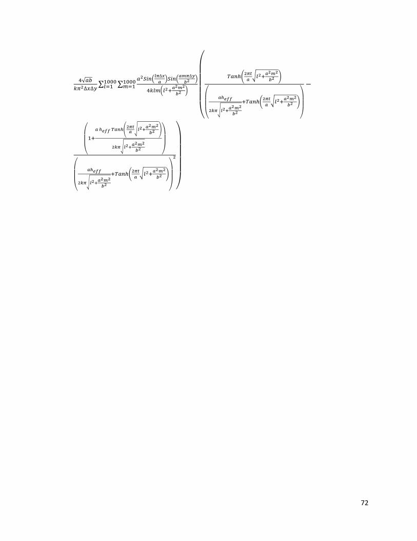
72

4√𝑎𝑏


𝑎2𝑆𝑖𝑛(𝑙𝜋∆𝑥

𝑎)𝑆𝑖𝑛(

𝑎𝑚𝜋∆𝑦

𝑏2)

4𝑘𝑙𝑚(𝑙2+𝑎2𝑚2

𝑏2)

(


𝑎√𝑙2+

𝑎2𝑚2

𝑏2)

(

𝑎ℎ𝑒𝑓𝑓


𝑏2


𝑎√𝑙2+

𝑎2𝑚2

𝑏2)

)

−1000𝑚=1

1000𝑙=1

(

1+


𝑎2𝑚2

𝑏2)


𝑏2)

(

𝑎ℎ𝑒𝑓𝑓


𝑏2


𝑎√𝑙2+

𝑎2𝑚2

𝑏2)

)

2

)

an investigation of a flat plate oscillating heat pipe …

Documents