an isoperimetric inequality for an integral operator …marzuola/eqtorus_final.pdf · an...
TRANSCRIPT

AN ISOPERIMETRIC INEQUALITY FOR
AN INTEGRAL OPERATOR ON FLAT TORI
BRAXTON OSTING, JEREMY MARZUOLA, AND ELENA CHERKAEV
Abstract. We consider a class of Hilbert-Schmidt integral operators with an isotropic, stationary kernel
acting on square integrable functions defined on flat tori. For any fixed kernel which is positive and decreas-
ing, we show that among all unit-volume flat tori, the equilateral torus maximizes the operator norm andthe Hilbert-Schmidt norm.
1. Statement of results and discussion
Let Ta,b be a unit-volume flat torus with parameters (a, b) ∈ U ⊂ R2 with
(1) U :={
(a, b) ∈ R2 : b > 0, a ∈ [0, 1/2], and a2 + b2 ≥ 1}.
The parametrization we use is fairly standard and will be introduced in detail in Section 2. The set Uis illustrated in Figure 1 and, in this notation, the square torus has parameters (a, b) = (0, 1) and the
equilateral torus has parameters (a, b) =(
12 ,√
32
). Consider the integral operator Af : L2(Ta,b) → L2(Ta,b)
with isotropic stationary kernel, f : R→ R, given by
Afψ(x) :=
∫Ta,b
f(d2(x,y)
)ψ(y) dy.
Here, d is the geodesic distance on Ta,b and f is evaluated at the squared distance. If
(2)
∫Ta,b
∫Ta,b
|f(d2(x,y)
)|2 dxdy <∞,
then Af is a Hilbert-Schmidt integral operator, hence bounded and compact. Let ‖ · ‖L2(Ta,b) and ‖ · ‖H.S.denote the L2(Ta,b)→ L2(Ta,b) and Hilbert-Schmidt operator norms respectively.
Theorem 1.1. Let f be a fixed positive and non-increasing function satisfying (2). Among unit-volumeflat tori, Ta,b, the equilateral torus is a maximizer of both ‖Af‖L2(Ta,b) and ‖Af‖H.S.. The square torus is acritical point of these spectral quantities. If f is additionally assumed to be decreasing, then the equilateraltorus is the unique minimizer and the square torus is a saddle point of these spectral quantities.
Remark 1.2. A self-contained proof of Theorem 1.1 is given in Section 2. The result that the equilateral torusis a maximizer follows from the Moment Lemma of Laszlo Fejes Toth (see Remark 2.2). As we were unableto find an English version of this lemma in the literature, we provide a translated proof of in Appendix B.Here, we provide a self-contained, constructive proof of Theorem 1.1 that gives more precise insight intospectral optimization problems over the family of flat tori considered. In particular, we emphasize that weobserve the square torus as a saddle point of the reported spectral quantities and gain fairly precise controlover the dependence on the parameters (a, b).
To prove Theorem 1.1, we obtain explicit expressions for ‖Af‖L2(Ta,b) and ‖Af‖H.S. and then use arearrangement method to show that the equilateral torus is maximal. The proof involves the rearrangementof a six-sided polygon with some special properties. Generally speaking, rearrangement of polygons isdifficult, as symmetrization typically destroys polygonal structure, e.g., Steiner symmetrization introducesadditional vertices. In fact, as far as we know, it remains an open problem to prove the conjecture of George
Date: June 9, 2016.2010 Mathematics Subject Classification. 35P05, 45P05, 52B60, 58C40.Key words and phrases. Isoperimetric Inequality, Flat torus, Equilateral Torus, Hilbert-Schmidt Integral Operator.
1

a0
b
10.5
equilateraltorus
rect
an
gula
rto
ri
squaretorus
Figure 1. The set U , defined in (1), is shaded.
Polya and Gabor Szego [PS51, Section 7], that among all N -gons of given area for fixed N ≥ 5, the regularone has the smallest first Laplace-Dirichlet eigenvalue; see also [Hen06, Open Problem 2]. Theorem 1.1 ismost similar to a result of Marcel Berger, which shows that the maximum first eigenvalue of the Laplace-Beltrami operator over all flat tori is attained only by the equilateral torus [Ber73; KLO16]. See also thework of Baernstein [Bae97], in which heat kernels are studied over flat tori. Finally, the present work can insome sense be seen as complementary to the lattice optimization problems of minimizing the Epstein zetaenergy [Ran53; Cas59; Dia64; Enn64] and the theta energy [Mon88], both of which are minimized by thetriangular lattice.
2. Proof of Theorem 1.1
Let B ∈ R2×2 have linearly independent columns. The lattice generated by the basis B is the set ofinteger linear combinations of the columns of B, L(B) = B(Z2). Let B and C be two lattice bases. We recallthat L(B) and L(C) are isometric if there is a unimodular1 matrix U such that B = CU . The followingproposition gives a parameterization of the space of two-dimensional, unit-volume lattices modulo isometry.
Proposition 2.1. Every two-dimensional lattice with volume one is isometric to a lattice, La,b, parameter-ized by the basis
Ba,b =
(1√b
a√b
0√b
),
where the parameters a, b ∈ U and U is defined in (1) and illustrated in Figure 1.
For (a, b) ∈ U , we refer to La,b = Ba,b(Z2) as the lattice generated by vector (a, b). A proof of thisProposition 2.1 is standard, but for completeness is provided in Appendix A.
A flat torus is a torus with a metric inherited from its representation as the quotient R2/L, where L isa lattice. Tori are isometric iff the matrices of the generating lattices are equivalent via left multiplication
1A matrix A ∈ Zn×n is unimodular if detA = ±1.
2

by an orthogonal matrix, see [Wol78]. Hence, by Proposition 2.1 a parameterization of the unit volume flattori is given by
Ta,b = R2/La,b, (a, b) ∈ U.Let Λa,b = B−ta,b(Z2) be the dual lattice of La,b, namely the set of all vectors whose inner products with
each vector in La,b is an integer,
Λa,b = {y ∈ R2 : y · x ∈ Z for all x ∈ La,b};see for instance [RS78, Chapter XIII.16]. For k ∈ Λa,b, a computation using lattice Fourier analysis showsthat
Af eık·x =
∫Ta,b
f(d2(y, c)
)e−ık·ydy eık·x ≡ γf (k) eık·x,
where c = ca,b is the center of Ta,b. For the representative parallelogram of Ta,b with (0, 0) in the bottom
left corner, we have ca,b =(
(a+ 1)/(2√b), 1/(2
√b))
. Thus Af is diagonalized by the Fourier Transform
with eigenvalues given by γf (k), k ∈ Λa,b. We observe that
γf (k) =
∫Ta,b
f(d2(x, c)
)e−ık·xdx ≤
∫Ta,b
f(d2(x, c)
)dx = γf (0),
and thus the largest eigenvalue of Af is given by γf (0),
(3) ‖Af‖L2(Ta,b) =
∫Ta,b
f(d2(x, c)
)dx.
Equation (3) also follows from Young’s inequality. We also compute
‖Af‖H.S. =
∫Ta,b
f2(d2(x, c)
)dx,(4)
where we used the assumption that |Ta,b| = 1.From (3) and (4), the proof of Theorem 1.1 requires us to solve the following optimization problem
(5) max(a,b)∈U
J(a, b) where J(a, b) :=
∫Ta,b
f(d2(x, c)
)dx.
We tile the plane with the torus Ta,b and consider the Dirichlet-Voronoi cell for the origin, Da,b, definedas the set of points closer to the origin than any of the other lattice points. We define
y1(x) :=1
2√b
((1− a)2
b+ b
)+
1− ab
x,(6)
y2(x) :=1
2√b
(a2
b+ b
)− a
bx,(7)
and
(8) x1 :=1
2√b, x2 :=
a− 1/2√b
.
The Dirichlet-Voronoi cell for the origin can be explicitly written
Da,b = {(x, y) ∈ R2 : x ∈ [−x1, x1], y ≤ y1(x) ∀x ∈ [−x1, x2], y ≤ y2(x) ∀x ∈ [x2, x1],
y ≥ −y2(−x) ∀x ∈ [−x1,−x2], y ≥ −y1(−x) ∀x ∈ [−x2, x1]}.This Dirichlet-Voronoi cell is illustrated in Figure 2 for a square torus (left), a torus Ta,b with (a, b) = (0.2, 1.2)(center), and an equilateral torus (right). The vertices of the Dirichlet-Voronoi cell are concyclic; theDirichlet-Voronoi cell is a cyclic polygon with four vertices if a = 0 and six vertices if a ∈ (0, 1/2]. Theinradius is given by
r1 :=1
2√b
and the circumradius is given by
r2 :=
√(a2 + b2) ((a− 1)2 + b2)
4b3> r1.
3

Figure 2. An illustration of Da,b, the Dirichlet-Voronoi cell of the origin, for a squaretorus (left), a torus with (a, b) = (0.2, 1.2) (center), and an equilateral torus (right). Thevertices of the Dirichlet-Voronoi cell are concyclic and both the incircle and circumcircle areplotted.
For (a, b) ∈ U , the objective function, J(a, b), in (5) can be rewritten as an integral over the Dirchlet cellwhere the distance is now simply the Euclidean distance to the origin,
(9) J(a, b) =
∫Da,b
f(‖x‖2
)dx, (a, b) ∈ U.
Remark 2.2. From (9), Theorem 1.1 now follows from the Moment Lemma of Laszlo Fejes Toth, see TheoremB.6 or, for example, [Fej72, p. 198], [Fej73], or [Gru99], [BC10]. Namely, if f is a non-increasing functionand D(p) any Dirichlet-Voronoi cell of a point p ∈ R2 with 6 vertices, we have
∫D(p)
f(‖x− p‖2
)dx ≤
∫R
f(‖x‖2
)dx,
where R is the regular 6-gon centered at the origin with |R| = |D(p)|. This result is intuitive; since fis a positive and decreasing function, the optimal torus will be described by the parameters (a, b) ∈ Usuch that the Dirichlet-Voronoi cell is most concentrated about the origin. The equilateral lattice has theDirichlet-Voronoi cell with the most symmetry, so intuitively it is the maximizer.
Remark 2.3. We will prove the statement in Theorem 1.1 which assumes that f is decreasing; the statementfor f non-increasing can be proved similarly.
We complete the proof by showing that when we continually rearrange the Dirichlet-Voronoi cell, firstincreasing a and then decreasing b while keeping (a, b) ∈ U , the objective function is strictly increasing. Thisimplies that the maximum is attained uniquely by the equilateral torus. We proceed with a few preliminaryresults, and then put them together to finish the proof.
We use the polar symmetry (x ∈ Ta,b =⇒ −x ∈ Ta,b) to reduce the integral in (9) to the upper halfplane. We obtain
(10) J(a, b) = 2
∫ x2
−x1
∫ y1(x)
0
f(x2 + y2
)dydx+ 2
∫ x1
x2
∫ y2(x)
0
f(x2 + y2
)dydx, (a, b) ∈ U.
4

We compute the partial derivatives of J(a, b). The partial derivative of J(a, b) with respect to the parametera, is given by
∂a1
2J(a, b) =
∫ x2
−x1
f(x2 + y2
1(x))
(∂ay1(x)) dx+
∫ x1
x2
f(x2 + y2
2(x))
(∂ay2(x)) dx
=1
b
∫ x2
−x1
f(x2 + y2
1(x))(a− 1√
b− x)dx+
1
b
∫ x1
x2
f(x2 + y2
2(x))( a√
b− x)dx
= −1
b
∫ x2
−x1
f(x2 + y2
1(x))(
x− a− 1√b
)dx(11)
+1
b
∫ a√b
x2
f(x2 + y2
2(x))( a√
b− x)dx− 1
b
∫ x1
a√b
f(x2 + y2
2(x))(
x− a√b
)dx.
The partial derivative of J(a, b) with respect to the parameter b is
∂b1
2J(a, b) =− 1
2b32
∫ y2(x1)
0
f
(1
4b+ y2
)dy
+
∫ x2
−x1
f(x2 + y2
1(x))
(∂by1(x)) dx+
∫ x1
x2
f(x2 + y2
2(x))
(∂by2(x)) dx.(12)
Lemma 2.4. For any integrable function f , ∂aJ(a, b) = 0 if either a = 0 or a = 12 . Furthermore, the square
(a, b) = (0, 1) and equilateral torus (a, b) =(
12 ,√
32
)are critical points of J(a, b).
Proof. Setting a = 0 we have that x2 = −x1 and y2(x) =√b
2 . From (11), we obtain
∂a1
2J(a, b) = −1
b
∫ x1
−x1
f
(x2 +
b
4
)x dx = 0.
If, additionally b = 1, we have from (12) that
∂b1
2J(a, b) = −1
2
∫ x1
0
f
(1
4+ y2
)dy +
∫ x1
−x1
f
(x2 +
1
4
)1
4dx = 0.
For a = 12 , we have x2 = 0 and y2(x) = 1
2√b
(14b + b
)− 1
2bx = y1(−x). From (11), we obtain
∂a1
2J(a, b) = −1
b
∫ 0
−x1
f(x2 + y2
1(x))( 1
2√b
+ x
)dx+
1
b
∫ x1
0
f(x2 + y2
1(−x))( 1
2√b− x)dx
= 0.
If, additionally b =√
32 , then we have y2(x) = x1
b −12bx = y1(−x) and
∂by2(x) =1
2b2x = (∂by1)(−x).
Hence,
∂b1
2J(a, b) =− 1
2b32
∫ x12b
0
f
(1
4b+ y2
)dy +
1
b2
∫ x1
0
f(x2 + y2
2(x))xdx.
Looking at the second integral, we complete the square in the argument of f ,
x2 + y22(x) =
1
b2
(x− x1
2
)2
+1
4b.
Now letting z = 1b
(x− x1
2
), the second integral can then be rewritten
1
b2
∫ x1
0
f(x2 + y2
2(x))xdx =
1
b2
∫ x12b
− x12b
f
(1
4b+ z2
)(bz +
x1
2
)bdz
=x1
b
∫ x12b
0
f
(1
4b+ z2
)dz,
which perfectly cancels the first integral. Thus, ∂bJ(a, b) = 0. �5

Figure 3. An illustration of how the Dirichlet-Voronoi cell, Da,b, changes between (a, b) =(0.2, 1) and (a, b) = (0.3, 1).
Lemma 2.5. For any positive and decreasing function f , ∂aJ(a, b) > 0 for (a, b) ∈ U with a ∈ (0, 1/2).
Proof. Fix (a, b) ∈ U with a ∈ (0, 1). From (11), we write
∂a1
2J(a, b) ≡ −I1 + I2 − I3,
where
I1 :=1
b
∫ x2
−x1
f(x2 + y2
1(x))(
x− a− 1√b
)dx
I2 :=1
b
∫ a√b
x2
f(x2 + y2
2(x))( a√
b− x)dx
I3 :=1
b
∫ x1
a√b
f(x2 + y2
2(x))(
x− a√b
)dx.
The integrals defined in I1, I2 and I3 are non-negative. These integrals have a nice geometric picture, whichwe illustrate in Figure 3. Here, we plot the Dirichlet-Voronoi cell for b = 1 and two different values of a:a = 0.2 and a = 0.3. The three integrals each correspond to a piece of the Dirichlet-Voronoi cell that is beingadded or removed as the parameter a is varied. We now transform each interval of integration to [−1, 1] sowe can compare the magnitude of the three integrals.
Integral 1. Let x = − 1−a2√b− a
2√bz. Making this change of variables in I1, we obtain
I1 =1
b
∫ 1
−1
a(1− a− az)4b
f
(b2 + (1− a)2
4b3(b2 + a2z2)
)dz
Define the argument of f ,
A1(z) :=b2 + (1− a)2
4b3(b2 + a2z2).
Note that A1(z) is even in z, so the term that is linear in z is zero. Thus, we can write
I1 =1
16b2
∫ 1
−1
4a(1− a) f (A1(z)) (1− z) dz.
6

It will later be clear why we want the coefficient to contain the term (1− z).
Integral 2. Let x = 4a−14√b
+ 14√bz. Making this change of variables in I2, we obtain
I2 =1
16b2
∫ 1
−1
f (A2(z)) (1− z) dz,
where the argument of f is defined
A2(z) :=a2 + b2
16b3(4b2 + (1− 2a− z)2
).
Integral 3. Let x = 1+2a4√b− 1−2a
4√bz. Making this change of variables in I3, we obtain
I3 =1
16b2
∫ 1
−1
(1− 2a)2 f (A3(z)) (1− z) dz,
where the argument of f is defined
A3(z) :=a2 + b2
16b3
(4b2 + ((1− 2a)z − 1)
2).
Putting the pieces together. Note that the coefficients in I1 and I3 sum to 1,
4a(1− a) + (1− 2a)2 = 1.
Breaking I2 into two pieces, we can write
∂a1
2J(a, b) = −I1 + I2 − I3
= [4a(1− a)I2 − I1] +[(1− 2a)2I2 − I3
]=
1
16b2
∫ 1
−1
4a(1− a) [f (A2(z))− f (A1(z))] (1− z) dz
+1
16b2
∫ 1
−1
(1− 2a)2 [f (A2(z))− f (A3(z))] (1− z) dz(13)
We will show that ∂aJ(a, b) > 0 by showing that both of the integrands in (13) are positive.
Claim: For every z ∈ (−1, 1), A1(z) ≥ A2(z).We compute
∂2z (A1(z)−A2(z)) =
b2 + (1− a)2
2b3a2 − a2 + b2
8b3
=1
8b3(4a2(1− 2a)−
(a2 + b2
) (1− (2a)2
))=
1− 2a
8b3(4a2 −
(a2 + b2
)(1 + 2a)
)= −1− 2a
8b3(2a(a2 + b2
)+ b2 − 3a2
)≤ 0
as b2 ≥ 3a2. Since
A1(−1)−A2(−1) =b2 + (1− a)2
4b3(a2 + b2
)− a2 + b2
4b3
(b2 + (1− a)
2)
= 0,
A1(1)−A2(1) =(1− 2a)
(a2 + b2
)4b3
≥ 0,
and A1(z)−A2(z) is a concave function, it follows that A1(z)−A2(z) ≥ 0 for all z ∈ (−1, 1).
Claim: For every z ∈ (−1, 1), A3(z) > A2(z).7

We compute
A3(z) =a2 + b2
16b3
[4b2 + ((1− 2a)z − 1)
2]
=a2 + b2
16b3
[4b2 + (1− 2a− z)2
+ 4a(1− a)(1− z2)]
>a2 + b2
16b3
[4b2 + (1− 2a− z)2
]= A2(z).
Since f is a decreasing function, these two claims show that the integrands in (13) are strictly positivefor every z ∈ (−1, 1). Thus, ∂aJ(a, b) > 0. �
Lemma 2.6. Let a = 12 and b >
√3
2 and f a positive and decreasing function. Then ∂bJ(a, b) < 0.
Proof. In (12), we computed the partial derivative of J(a, b) with respect to the parameter b. For a = 12 , we
have x2 = 0,
y2(x) =1
2√b
(1
4b+ b
)− 1
2bx = y1(−x),
and
∂by2(x) =1
4√b
(1− 3
4b2
)+
1
2b2x = (∂by1)(−x).
We obtain
∂b1
2J(a, b) =− 1
2b32
∫ y2(x1)
0
f
(1
4b+ y2
)dy
+
∫ 0
−x1
f(x2 + y2
2(−x))
(∂by2(−x)) dx+
∫ x1
0
f(x2 + y2
2(x))
(∂by2(x)) dx
=− 1
2b32
∫ y2(x1)
0
f
(1
4b+ y2
)dy + 2
∫ x1
0
f(x2 + y2
2(x))
(∂by2(x)) dx(14)
We denote the second integral in (14), by
K2 := 2
∫ x1
0
f(x2 + y2
2(x))
(∂by2(x)) dx.
Making the change of variables,
z =4b2 − 1
2b
(x− x1
2
),
we compute
x2 + y22(x) =
1 + 4b2
16b+
1 + 4b2
(4b2 − 1)2z2 and ∂by2(x) =
4b2 − 1
16b52
+z
b(4b2 − 1),
to obtain
K2 = 2
∫ z1
−z1f
(1 + 4b2
16b+
1 + 4b2
(4b2 − 1)2z2
)(4b2 − 1
16b52
+z
b(4b2 − 1)
)2b
4b2 − 1dz
where z1 := 4b2−1
8b32
. The term involving the z in the square brackets is an odd function and the term involving
the constant is even so we have
K2 =1
2b32
∫ z1
0
f
(1 + 4b2
16b+
1 + 4b2
(4b2 − 1)2z2
)dz
Finally noting that z1 = y2(x1), we obtain from (14),
∂b1
2J(a, b) =
1
2b32
∫ z1
0
f
(1 + 4b2
16b+
1 + 4b2
(4b2 − 1)2z2
)− f
(1
4b+ z2
)dz.
8

But for b ≥√
32 , a simple calculation shows that
1
4b+ z2 ≤ 1 + 4b2
16b+
1 + 4b2
(4b2 − 1)2z2, z ∈ (0, z1).
Thus, if f is a positive and decreasing function, this implies that ∂bJ(a, b) < 0 for a = 12 and b >
√3
2 . �
Proof of Theorem 1.1. The preceding results are now put together as follows. We start with a flat torus, Ta,bwith (a, b) ∈ U . By Lemma 2.5, by continually rearranging the torus by increasing a, the objective functionis strictly increasing. We stop when a = 1
2 . We then continually rearrange the torus by decreasing b and by
Lemma 2.6, the objective function is again strictly increasing. We stop when b =√
32 . Thus the maximum
is attained by the equilateral torus. This completes the proof. �
Remark 2.7. Interestingly, the square torus is a saddle point of J(a, b). This is a similar phenomenon tothat observed by spectral properties of the Laplacian on a Bravais Lattice, see [OM16].
Appendix A. Proof of Proposition 2.1
Consider an arbitrary lattice with unit volume. We first choose the basis vectors so that the angle betweenthem is acute. After a suitable rotation and reflection, we can let the shorter basis vector (with length 1√
b)
be parallel with the x axis and the longer basis vector (with length√
a2
b + b =√
1b (a2 + b2) ≥
√1b ) lie in
the first quadrant. Multiplying on the right by a unimodular matrix,
(1 10 1
), we compute(
1√b
a√b
0√b
)(1 10 1
)=
(1√b
a+1√b
0√b
).
Since this is equivalent to taking a 7→ a + 1, it follows that we can identify the lattices associated to thepoints (a, b) and (a+ 1, b). Thus, we can restrict the parameter a to the interval [0, 1/2] by symmetry. Fora complete picture of this restriction and how the symmetry naturally arises, see [KLO16, Proposition 3.2and Figure 3]. For more on flat tori, see also [Mil64; GT10; LS11]. �
Appendix B. A Translation of the Proof of The Fejes Toth Moment Lemma
Here we translate and discuss Laszlo Fejes Toth’s proof of his Moment Theorem, which was published inGerman [Fej72] and Russian [Fej58]. Other references for the Moment Theorem include [Fej73] where a sumof moments theorem is proved, [Gru99] where the sum of moments theorem is proved using the MomentLemma below, [BC10] where a new version of the Moment Theorem appears with quadratic forms insteadof moments, and [Gru07] which contains a very nice summary of Moment type results. See also [BPT14] foran application of the Moment Theorem to block copolymer structures. This is by no means a complete listof relevant references for the proofs and development of the Moment Theorem, but gives some idea of itslong and important history.
We present also Laszlo Fejes Toth’s proof of his Moment Lemma, as given in [Fej63]. This Lemma is alsostated, but not proven in [Fej73; Gru99; Gru07]. Some of the arguments and notation have been slightlymodified from the original proof for clarification.
Theorem B.1. The Moment Theorem, [Fej72, p.80] Assume f : [0,∞) → R is a non-increasing function.Let p1, . . .pn be n points in the plane and C ⊂ R2 a convex hexagon. Let d(p) = mini ‖p − pi‖ be thedistance from the point p to the set {pi}ni=1. It holds that
(15)
∫C
f (d(p)) dp ≤ n ·∫σ
f (‖p‖) dp
where σ is a regular hexagon with volume |C|n and center o.9

Toth’s proof of Proposition B.1 relies on the Voronoi partition of the convex set C ⊂ R2 by the points{pi}ni=1 and a careful analysis of the resulting partition components. Namely a rearrangement argument isused to compare each partition component to a ball which circumscribes the regular hexagon σ. The proofuses the following three lemmas, which we first prove. We note that Lemmas B.2 and B.3 are also proven in[Imr64] and stated (but not proven) in [Fej63].
Lemma B.2. [Fej72, Lemma 1, p.82] Assume f : [0,∞) → R is a non-increasing function. Let K ⊂ R2
be a ball centered at o. Let S = S(s) be a circular segment parameterized by its volume, s = |S|. Then thefunction
ω(s) :=
∫S(s)
f (‖x‖) dx, 0 ≤ s < |K|/2
is convex.
Proof. Consider the circular segments with volumes s1 < s∗1 < s2 < s∗2 with s∗i − si = ε for i = 1, 2. Let ∆Sifor i = 1, 2 denote the (nearly trapezoidal) regions S(s∗i )\S(si). From Figure 4 it is clear that correspondingpoints x1 ∈ ∆S1 and x2 ∈ ∆S2 satisfy ‖x1‖ > ‖x2‖. Noting that |∆S2| = |∆S1| and using the monotonicityof f , we have that
ω(s∗1)− ω(s1) =
∫∆S1
f (‖x‖) dx ≤∫
∆S2
f (‖x‖) dx = ω(s∗2)− ω(s2).
Dividing both sides by ε and taking the limit s∗i → si for i = 1, 2, i.e., ε→ 0, we have that ω′(s1) ≤ ω′(s2)which shows that ω is a convex function. �
o S(s)
K
o
K
∆S2
x2
∆S1
x1
Figure 4. Illustrations for the statement and proof of Lemma B.2. See [Fej72, Fig.78].
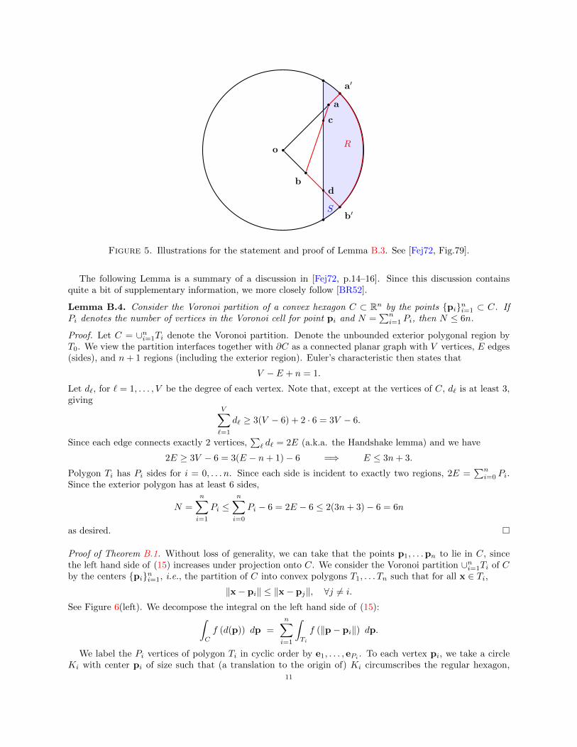
Lemma B.3. Assume f : [0,∞)→ R is a non-increasing function. Let a and b be two points contained inthe ball K centered at o. Let a′ and b′ be the points at the respective intersections between the rays −→oa and−→ob with ∂K. Let R ⊂ K denote the region enclosed by the path defined by the segments a′a, ab, bb′, andthe circular arc ∠b′a′. Let S = S(s) denote the circular segment with volume s = |R|. It holds that
ω(s) :=
∫S
f (‖x‖) dx ≤∫R
f (‖x‖) dx.
Proof. As in Figure 5, position the circular segment, S, so that there are two points, c and d, at ∂S ∩ ∂Requidistant to o. Since, aside from c and d, each point of the region R \ S is closer to o then each point inS \R, using the monotonicity of f , we have the inequality∫
R
=
∫R∩S
+
∫R\S
≥∫S∩R
+
∫S\R
=
∫S
,
where the integrand for each of these integrals is f (‖x‖) dx. �10
o
a′
a
b′
b
R
S
c
d
Figure 5. Illustrations for the statement and proof of Lemma B.3. See [Fej72, Fig.79].
The following Lemma is a summary of a discussion in [Fej72, p.14–16]. Since this discussion containsquite a bit of supplementary information, we more closely follow [BR52].
Lemma B.4. Consider the Voronoi partition of a convex hexagon C ⊂ Rn by the points {pi}ni=1 ⊂ C. IfPi denotes the number of vertices in the Voronoi cell for point pi and N =
∑ni=1 Pi, then N ≤ 6n.
Proof. Let C = ∪ni=1Ti denote the Voronoi partition. Denote the unbounded exterior polygonal region byT0. We view the partition interfaces together with ∂C as a connected planar graph with V vertices, E edges(sides), and n+ 1 regions (including the exterior region). Euler’s characteristic then states that
V − E + n = 1.
Let d`, for ` = 1, . . . , V be the degree of each vertex. Note that, except at the vertices of C, d` is at least 3,giving
V∑`=1
d` ≥ 3(V − 6) + 2 · 6 = 3V − 6.
Since each edge connects exactly 2 vertices,∑` d` = 2E (a.k.a. the Handshake lemma) and we have
2E ≥ 3V − 6 = 3(E − n+ 1)− 6 =⇒ E ≤ 3n+ 3.
Polygon Ti has Pi sides for i = 0, . . . n. Since each side is incident to exactly two regions, 2E =∑ni=0 Pi.
Since the exterior polygon has at least 6 sides,
N =
n∑i=1
Pi ≤n∑i=0
Pi − 6 = 2E − 6 ≤ 2(3n+ 3)− 6 = 6n
as desired. �
Proof of Theorem B.1. Without loss of generality, we can take that the points p1, . . .pn to lie in C, sincethe left hand side of (15) increases under projection onto C. We consider the Voronoi partition ∪ni=1Ti of Cby the centers {pi}ni=1, i.e., the partition of C into convex polygons T1, . . . Tn such that for all x ∈ Ti,
‖x− pi‖ ≤ ‖x− pj‖, ∀j 6= i.
See Figure 6(left). We decompose the integral on the left hand side of (15):∫C
f (d(p)) dp =
n∑i=1
∫Ti
f (‖p− pi‖) dp.
We label the Pi vertices of polygon Ti in cyclic order by e1, . . . , ePi . To each vertex pi, we take a circleKi with center pi of size such that (a translation to the origin of) Ki circumscribes the regular hexagon,
11

p
C
p1e5
e4
pi
p3
p4
ei
Ri1
Ri2 Ri
3
e3
Ri5
e2
p2
Kσ
K
HU
Figure 6. Illustrations for the proof of Theorem B.1. See [Fej72, Fig.80].
σ, with volume |σ| = |C|/n. Let Ri` ⊂ Ki \ Ti for ` = 1, . . . , Pi be a region associated to the `-th edge ofVoronoi cell i as illustrated in Figure 6(left). Of course, we allow for Ri` to be empty. Additionally we defineT ′i = Ti \Ki, which could also be empty. We then decompose the integral∫
Ti
=
∫Ki
+
∫T ′i
−Pi∑`=1
∫Ri
`
where the integrands are all f (‖p− pi‖) dp. Hereinafter we will frequently suppress integrands to simplifyexposition. Note that the first integral is the same for all i = 1, . . . , n,∫
Ki
f (‖p− pi‖) dp =
∫K
f (‖p‖) dp.
Next, we consider the rearrangement of each region Ri` into a circular segment S = S(si`) with volumesi` = |S| = |Ri`|. Using Lemma B.3, we have∫
Ri`
f (‖p− pi‖) dp ≥ ω(|Ri`|
),
giving ∫Ti
≤∫K
+
∫T ′i
−Pi∑`=1
ω(|Ri`|
).
Now summing over i = 1, . . . , n, we have that∫C
f (d(p)) dp =
n∑i=1
∫Ti
≤ n
∫K
+
n∑i=1
∫T ′i
−n∑i=1
Pi∑`=1
ω(|Ri`|
).
Let N =∑ni=1 Pi. Using the convexity of ω (Lemma B.2) and Jensen’s inequality, we have∫
C
f (d(p)) dp ≤ n
∫K
+
n∑i=1
∫T ′i
− N · ω
(1
N
n∑i=1
Pi∑`=1
|Ri`|
).
Letting T ′ = ∪ni=1T′i , we have that
|C| = n · |K| + |T ′| −n∑i=1
Pi∑`=1
|Ri`| =⇒ 1
N
n∑i=1
Pi∑`=1
|Ri`| =n · |K| + |T ′| − |C|
N.
Since ω(0) = 0 and ω is an increasing, convex function it follows that ω(x)x is a continuous and increasing
function. Using Lemma B.4, we have that N ≤ 6n which implies
(16)
∫C
f (d(p)) dp ≤ n
∫K
+
n∑i=1
∫T ′i
− 6n · ω(n · |K|+ |T ′| − |C|
6n
).
12

Let H be one of the circular segments in K \ σ. Recalling |C| = |σ|n, we have
H = S(|H|) = S
(|K| − |σ|
6
)= S
(n · |K| − |C|
6n
).
We define U to be the set difference of two circular segments of K,
U = S
(n · |K|+ |T ′| − |C|
6n
)\H,
with volume |U | = |T ′|/6n; see Figure 6(right). We have
ω
(n · |K|+ |T ′| − |C|
6n
)= ω (|H|) +
∫U
f (‖p‖) dp.
From (16), we have that∫C
f (d(p)) dp ≤ n
[∫K
f (‖p‖) dp− 6 · ω (|H|)]
(17)
+
n∑i=1
∫T ′i
f (‖p− pi‖) dp − 6n ·∫U
f (‖p‖) dp
Noting that U ⊂ K, we have f(r) = min{f (‖p‖) : p ∈ U} where r is the radius of K and similarlyf(r) = max{f (‖p− pi‖) : p ∈ T ′i}. Thus, in the second line in the right hand side of (17), we have
n∑i=1
∫T ′i
f (‖p− pi‖) dp− 6n ·∫U
f (‖p− pi‖) dp ≤ f(r) · (|T ′| − 6n|U |) = 0.
The first line in the right hand side of (17) is exactly n ·∫σf (‖p‖) dp, which proves (15). �
Remark B.5. [Gru99] states the Moment Theorem for convex polygons with n = 3, 4, 5, or 6 vertices. Thisgeneralized statement follows from Proposition B.1 by introducing false vertices for n = 3, 4, or 5.
Theorem B.6 (The Moment Lemma, [Fej63]). Assume f : [0,∞) → R is a non-increasing function. LetC ⊂ R2 be a convex n-gon and σ the regular n-gon centered at the origin with |C| = |σ|. Then
(18)
∫C
f (‖p‖) dp ≤∫σ
f (‖p‖) dp.
The moment Lemma for hexagons follows from the Moment Theorem when n = 1. We also mentionthat Peter M. Gruber’s proof of the Moment Theorem relies on the Moment Lemma [Gru99; Gru07]. Thefollowing proof, which closely follows [Fej63], is very similar to the proof of the Moment Theorem.
Proof of Theorem B.6. We may assume that C contains the origin. Otherwise, by translating C towardsthe origin the integral on the left side of (18) would increase. Let K denote the circle that circumscribes σ.Define R` ⊂ K, ` = 1, . . . , n to be the regions as in Figure 7 so that ∪`R` = K \ C. We allow some of theR` to be empty. Define C ′ = C \K. We can then write∫
C
=
∫K
−∑`
∫R`
+
∫C′
where the integrands here and below are understood to be f (‖p‖) dp. Using Lemma B.3, we have that∫R`≥ ω(|R`|). Using the convexity of ω (Lemma B.2) and Jensen’s inequality, we then have that∫
C
≤∫K
−∑i
ω(|R`|) +
∫C′≤∫K
−nω
(1
n
∑i
|R`|
)+
∫C′
Let H be one of the circular segments in K \ σ. Using the equality of the volumes
|C| = |K| −∑`
|R`|+ |C ′| and |σ| = |K| − n|H|
13

K
C
R1
R2
R3
R5
C ′
Figure 7. Illustration for the proof of Theorem B.6.
we obtain1
n
∑`
|R`| =1
n|C ′|+ |H|.
As in Figure 6(right), let U be the set difference between the two circular segments of K,
U = S
(1
n|C ′|+ |H|
)\H,
we have that
ω
(1
n
∑`
|R`|
)= ω(|H|) +
∫U
.
Using the fact that all points in U are closer to the origin then points in C ′ and the monotonicity of f , wehave that n
∫U≥∫C′ . Finally, observing that
∫σ
=∫K−n · ω(|H|), we conclude that∫
C
≤∫K
−n ·(ω (|H|) +
∫U
)+
∫C′≤∫σ
,
as desired. �
Acknowledgments
The authors wish to thank Mikael Rechtsman and Sylvia Serfaty for very helpful conversations during thepreparation of this manuscript. BO was supported in part by U.S. NSF DMS-1461138. JLM was supportedin part by U.S. NSF DMS-1312874 and NSF CAREER Grant DMS-1352353.
References
[Bae97] A. Baernstein II. “A minimum problem for heat kernels of flat tori”. In: Extremal RiemannSurfaces, Contemp. Math 201 (1997), pp. 227–243.
[BR52] R. P. Bambah and C. A. Rogers. “Covering the Plane with Convex Sets”. In: Journal of theLondon Mathematical Society s1-27.3 (1952), pp. 304–314.
[Ber73] M. Berger. “Sur les premieres valeurs propres des varietes Riemanniennes”. In: Compositio Math-ematica 26.2 (1973), pp. 129–149.
[BC10] K. J. Boeroeczky and B. Csikos. “A new version of L. Fejes Toth’s Moment Theorem”. In: StudiaScientiarum Mathematicarum Hungarica 47.2 (2010), pp. 230–256.
14
[BPT14] D. P. Bourne, M. A. Peletier, and F. Theil. “Optimality of the triangular lattice for a particlesystem with Wasserstein interaction”. In: Communications in Mathematical Physics 329.1 (2014),pp. 117–140.
[Cas59] J. W. S. Cassels. “On a problem of Rankin about the Epstein zeta function”. In: Proceedings ofthe Glasgow Mathematical Association. Vol. 4. 2. 1959, pp. 73–80.
[Dia64] P. H. Diananda. “Notes on two lemmas concerning the Epstein zeta function”. In: Proceedings ofthe Glasgow Mathematical Association. Vol. 6. 4. 1964, pp. 202–204.
[Enn64] V. Ennola. “A lemma about the Epstein zeta function”. In: Proceedings of the Glasgow Mathe-matical Association. Vol. 6. 1964, pp. 198–201.
[Fej73] G. Fejes Toth. “Sum of moments of convex polygons”. In: Acta Mathematica Hungaricae 24.3(1973), pp. 417–421.
[Fej58] L. Fejes Toth. Расположения на плоскости, на сфере и в пространстве. М., Физматлит,1958.
[Fej63] L. Fejes Toth. “On the Isoperimetric Property of the Regular Hyperbolic Tetrahedra”. In: AMagyar Tudomanyos Akademia Matematikai Kutato Intezetenk Kozlemenyei 8 (1963), pp. 53–57.
[Fej72] L. Fejes Toth. Lagerungen in der Ebene auf der Kugel und im Raum, 2nd ed. Vol. 65. Springer-Verlag, 1972.
[GT10] O. Giraud and K. Thas. “Hearing shapes of drums: Mathematical and physical aspects of isospec-trality”. In: Reviews of modern physics 82.3 (2010), p. 2213.
[Gru99] P. M. Gruber. “A short analytic proof of Fejes Toth’s theorem on sums of moments”. In: Aequa-tiones Mathematicae 58.3 (1999), pp. 291–295.
[Gru07] P. M. Gruber. Convex and Discrete Geometry. Springer, 2007.[Hen06] A. Henrot. Extremum Problems for Eigenvalues of Elliptic Operators. Birkhauser Verlag, 2006.[Imr64] M. Imre. “Kreislagerungen auf Flachen konstanter Krummung”. In: Acta Mathematica Academiae
Scientiarum Hungarica 15.1 (1964), pp. 115–121.[KLO16] C.-Y. Kao, R. Lai, and B. Osting. “Maximizing Laplace-Beltrami eigenvalues on compact Rie-
mannian surfaces”. In: to appear in ESAIM: Control, Optimisation and Calculus of Variations(2016).
[LS11] R. S. Laugesen and B. A. Siudeja. “Sums of Laplace eigenvalues: Rotations and tight frames inhigher dimensions”. In: Journal of Mathematical Physics 52.9 (2011), p. 093703.
[Mil64] J. Milnor. “Eigenvalues of the Laplace operator on certain manifolds”. In: Proceedings of theNational Academy of Sciences 51.4 (1964), pp. 542–542.
[Mon88] H. L. Montgomery. “Minimal theta functions”. In: Glasgow Mathematical Journal 30 (Jan. 1988),pp. 75–85.
[OM16] B. Osting and J. L. Marzuola. “Spectrally optimized point set configurations”. In: submitted(2016).
[PS51] G. Polya and G. Szego. Isoperimetric inequalities in mathematical physics. 27. Princeton Univer-sity Press, 1951.
[Ran53] R. A. Rankin. “A minimum problem for the Epstein zeta-function”. In: Proceedings of the GlasgowMathematical Association. Vol. 1. 1953, pp. 149–158.
[RS78] M. Reed and B. Simon. Methods of Modern Mathematical Physics: Vol.: 4.: Analysis of Operators.Academic press, 1978.
[Wol78] S. Wolpert. “The eigenvalue spectrum as moduli for flat tori”. In: Transactions of the AmericanMathematical Society 244 (1978), pp. 313–321.
Department of Mathematics, University of Utah, Salt Lake City, UT 84112, USAE-mail address: [email protected]
Department of Mathematics, University of North Carolina, Chapel Hill, NC 27599, USAE-mail address: [email protected]
Department of Mathematics, University of Utah, Salt Lake City, UT 84112, USA
E-mail address: [email protected]
15