an lntegrodifferential equation for rigid heat · pdf filean lntegrodifferential equation for...

JOURNAL OF MATHEMATICAL ANALYSIS AND APPLICATIONS 66, 313-332 (1978)

An lntegrodifferential Equation for

Rigid Heat Conductors with Memory

R. K. MILLER*

Iowa State University, Ames, Iowa 50011

Submitted by J. P. LaSallc

1. INTRODUCTION

The purpose of this paper is to study existence, uniqueness, and continuous dependence on parameters for solutions of the following system of integrodifferential equations:

e(t, x) = e, + a(O) O(t, x) + j:m a’(t - T) I~(T, x) dT,

4(t, X) = --k(O) Ve(t, x) - jt k’(t - T) VH(T, x) d7, -cc (1)

e’(t, 4 = -V . q(t, X) + r(t, x),

where 0 < t < co, x is a vector in a real n-dimensional set B, prime denotes differentiation with respect to the time variable t, V is the gradient operator with respect to x, and V * V = d is the Laplacian.

For K(O) = 0 these equations represent the linearized theory for heat flow in a rigid, isotropic, homogeneous material as proposed by Gurtin and Pipkin [12]. For k(0) > 0 the equations represent an alternate linearized theory proposed by Coleman and Gurtin [l]; see also Gurtin [13]. Nunziato [22, 231, Finn and Wheeler [6], and Nachlinger and Wheeler [21] h ave studied certain aspects of the general nonlinear theory as well as the problem of uniqueness and wave propagation for the linearized problem. Grabmueller [lo] gave a very general uniqueness proof for generalized solutions in a Sobelev space and proved existence theorems in certain special situations. Kremer [16] proved existence and uniqueness theorems for generalized distribution solutions. Grabmueller [ 1 l] also studied an inverse problem for (1).

The purpose of this note is to show in Section 2 that the appropriate history value problem of form (1) always has a generalized distribution solution which

* This work was done while the author was visiting at the Universitaet Karlsruhe (TH), Karlsruhe, Federal Republic of Germany. The author was supported by the Fulbright Commission and by the Iowa State University Faculty Leave Program.

313 OO22-247X/78/0662~313$02.OO/O

Copyright 0 1978 by Academic Press, Inc. All rights of reproduction in any form resented.

314 R. I(. MILLER

is not only unique but also depends continuously on the initial history and on the function r(t, .x). From this continuity it follows that the solutions obtained in [IO, Theorem 2.1.21 are the natural Hilbert space approximations of the general distribution solutions. The results in Section 2 are used to motivate the analysis in the rest of the paper. Section 3 isconcernedwith stability results. Conditions(S) and (E) when k(O) > 0 and (S’) when K(0) = 0 g ive necessary conditions on k(t) in order that (1) determine a stable model of the heat problem for all configuration&. Such necessary conditions for K(t) have not previously been noted. In Theorem 6 it is shown that stability of e(t, X) can be established by establishing stability for each mode separately. Some general consequences of stability are proved in Corollary 7 and Theorem 8. The results in Sections 4 and 5 show that for large classes of smooth r(t, X) and of smooth initial histories the generalized distribution solutions of (I) will actually be classical solutions. The transformation developed in Section 5 can be used to discuss the hyperbolic character of (1) when k(O) = 0 in a more satisfactory way than the earlier analysis in [2, 3,201.

We shall need some standard background material on existence, uniqueness and solution forms for Volterra integral equations on the real line. This material can be found collected in [17]. B ac kg round material for semigroups, Sobelev spaces, and functional analysis can be found in Krein [ 151, Pazy [24], or especially in Friedman [8].

2. RESULTS FOR DISTRIBUTION SOLUTIONS

The purpose of this section is to transform system (1) into an equivalent Volterra integrodifferential equation in Hilbert space. Background material and assumptions are given as needed. An existence, uniqueness, and continuity theorem is stated in this abstract setting. This continuity result is used to prove an approximation result, Theorem 2, which is the main result of this section.

Equations (1) are linearized about some nominal constant temperature 0, which will be taken to be zero. The rigid body will occupy a fixed open region B in n-dimensional space Rn (normally n = 1,2, or 3) and have boundary aB. The energy-temperature relation function a(t) and the heat conduction relation h(t) are both assumed continuous, to have a certain number of continuous derivatives, and to satisfy the following assumptions:

(HI) or(O) > 0 and either K(0) > 0, J : 2 or k(0) = 0, K’(0) > 0, J = 3.

U-W OL E C?r[O, co) and K E CJIO, CO).

W3) c#E,?(O, co)forl <j< JandNELl(O, oo)forl <j < J- I.

Assumption (H3) is stronger than needed for many of the results in the sequel. However, the full force of this assumption is used in returning from (3) or (4) below to system (1) above.

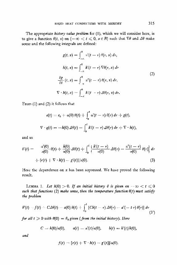
RIGID HEAT CONDUCTORS WITH MEMORY 315

The appropriate history value problem for (I), which we will consider here, is to give a function e(t, x) on {- 00 < t < 0, x E B} such that VO and .4B make sense and the following integrals are defined:

h(t, X) = 1” k’(t - T) ve(,, X) dT --J)

g (t, X) = 1” d(t - T) e(T, X) dT, --cc

(2)

v * h(t, a?) = 1” k’(t - T) &(T, X) dT. -cc

From (1) and (2) it follows that

e(t) = e, + 40) d(t) + it ~‘(t - T) O(T) dT + g(t),

v - q(t) = -k(o) de(t) - 1” k’(t - T) do(T) dr + v * h(t), 0

and so

Here the dependence on x has been supressed. We have proved the following result.

LEMMA 1. Let k(0) > 0. If an initial history 0 is given on - 03 < t < 0 such that functions (2) make sense, then the temperature function e(t) must satisfy the problem

e’(t) = f (t) f CAB(t) - a(O) e(t) + It [Cb(t - T) de(~) - a’(- t T) O(T)] dT 0

(3’) for all t 3 0 with 8(O) = B. given (from the initial history). Here

and

C = W)b(O), 44 = 4W(O>, b(t) = W/W,

f (4 = [r(t) + V . h(t) - ~Wll40)-

316 R. K. MILLER

The reader should note that the initialhistoryproblem (1) has been reformulated as an initiuE value problem (3’). The initial history e(t), -CC < t .< 0 and the given function r(t) have been used to determine initial conditions B0 and f(t) in the manner specified above. If r(t) were zero, it would be simplier to retain the initial history formulation. Since we wish to allow r(f) not zero, we think that (3’) will often be a more convenient form.

If k(0) = 0, then one can take another derivative in (3) to obtain the equation

a(0) qt, x) = -a’(O) V(t) - a”(0) O(t) + k’(0) m(t) (4

+ 6 [k”(t - T) &(T) - a”(t - T) e(T)] dT + [r’(t) + v * h’(t) - g”(t)].

The analog of Lemma 1 is the following result.

LEMMA 2. If k(0) = 0 and if th e initial history 8 is given on - ccj < t < 0 in such a manner that the functions g, g’, g”, h, V . h, and V * h’ make sense, then 9(t) must satisfy

d”(t) = f (t) + C,Af?(t) - a(0) e’(t) - a’(0) e(t)

+ f: [C,b,(t - T) D(T) - a”(t - T) O(T)] d7

for all t > 0 with e(O) = 0, and 0’(O) = v,, given. Here

(4’)

and

C, = k’(O)/‘a(O), b,(t) = k”(t)/k’(O),

f(t) = [r’(t) + V . h’(t) - g”(t>l/44~

As before, the initial history problem has been replaced by an initial valueproblem. This time the appropriate initial conditions are the quantities 0, , Q , and f(t).

We shall study a class of distribution solutions for (3) or for (4) under boundary conditions of the form

u(t, x) = 0 (O<t<co,xEaB) (5)

or of the form

b,(x) g (4 4 + b,(x) u(t, 4 = 0 (O<t<m,xEaB), (6)

where Y is the outward normal on aB, b,(x) and b,(x) are continuously differentiable on aB, and b,(x) f 0 for all x E 3B.


We use the Hilbert space X, = L2(B) of Lebesgue measurable functions $ on B such that

The space P(B) will be the set of all 4 E X1 such that $ has distribution partial derivatives through order K and these derivatives are all in L2(B). Let B = BU aB be the closure of the open set B, let C,,(B) be all P-smooth functions 4 with the compact support in B, and let H,,k(B) be the closure in H”(B) of C,,(B). Define X, = H:(B) and X, = X2 x X, .

If B is a bounded set and if the boundary aB is a P-smooth surface, then it is well known (see, e.g., [8, Chap. I, Sect. 191 that the operator d can be considered as a closed, linear operator on Xi whose domain is the closure of the set of all functions 4 E Ca(B) such that + satisfies boundary condition (5) or alternately boundary condition (6). The operator A = (R(O)/ol(O))d - (a’(O)/a(O))l will satisfy the following two conditions:

(H4) A generates a C,-semigroup on X, .

(H5) For h sufficiently large, U - A has a compact inverse on X1 . Moreover there exist simple eigenvalues h,(L+, < h,) and corresponding eigenfunctions & E C=(B) such that $m satisfies the given boundary conditions and A& = &,&. Th e set (&} is a complete, orthonormal set.

Assume that (Hl)-(H4) are true with K(0) > 0, J = 2. Let 6, andf(t) be given as in Lemma 1 with f : [0, co) + X1 continuous. The notion of “solution of (3’) satisfying the given initial and boundary conditions” has several possible inter- pretations. We could mean a ckzssical sohtion, that is that 0(t, z) is continuous on t > 0, x E B, 6’ satisfies the initial-boundary conditions at all relevant points (t, x), all requisite partial derivatives of 8 w.r.t. t and x exist and are continuous and (3’) is true for all (t, x) in (0, co) x B. In order to obtain existence and, in particular, continuity w.r.t. parameters it will be necessary to weaken this notion of solution considerably. By a distribution solution of (3’) satisfying initial condition 8, we shall mean a function 8: [0, co) -+ D(A), where D(A) is the domain of A in X, , such that e(t) and Ad(t) are continuous as maps from [0, co) to X, , e(O) = 8, and (3’) is true for all t E R +. By a generalized distribution solution satisfying initial condition 0, we shall mean a continuous function 8: [0, co) --f Xi such that e(O) = 0, and such that there is a sequence ok of distribution solutions such that

with the limit existing uniformly on compact subsets of the interval O<t<co.

The following result is a special case of Theorem 7.3 in [18].

318 R. K. MILLER

THEOREM 1. If (HI)-(H4) are true with k[O) >> 0 and J m:~: 2, then the following results are true:

(a) For each 8, E D(d) and each P-function f :[O, co) + -71, there is a unique distribution solution 0(t, 0, , f) of (3’) satisfying 0(0, B0 , f) = 8, .

(b) For each B,, E X, and each continuous function f: [0, 00) + Xl there is a unique generalized distribution solution 0(t, Bu , f) satisfying 0(0, 8, , f) = B. .

(c) 6(t, 8, ,f) vurys ContinuousZy with (t, B0 ,fJ. That is, given T > 0, there exists K 3 0 such that

II e(t, 4 ,f Iii G K(ll 4 ii + oy;> Ilf (09 for all t E [0, T]. ,.

The uniqueness part of Theorem 1 has already been proved by many authors. The most general uniqueness theorem is in [lo]. Kremer [16] has proved existence of generalized distribution solutions. The continuity result (c) is new (in the sense that it has not earlier been pointed out that the work in [ 181 could be applied to (1)). We remark that the constant K in (c) depends on T and of course on the fixed parameters C, a(t), and b(t). The value of K is independent of B,, and f (t). Since the existence of K follows from an application of the closed graph theorem, it is not possible to estimate its magnitude. (Similar remarks apply to Theorem 3 below.)

The continuity result (c) can be used to good advantage to justify an approximation scheme suggested by the work of Grabmueller [lo]. Indeed, the following result is true.

THEOREM 2. Suppose (Hl)-(H5) are true with k(0) > 0 and J = 2. Let 6, andf(t) be$xed with 6, E X, and f : [0, a) + X, continuous. If {A,} and (I&} are the sequences given in (H5) and ( , ) denotes the inner product in Xl define

Yk = (4 ,+r>, grw = <f(t) 4kh

4lm = 2 Yk4k 1 fm(t) = 2 g?S(t) A 7 k=l k=l

and

hdt) = f Yk(t)+k , k=l

where yk is the unique solution of the scalar problem

Y;(t) = gk@) + EAkC - @)I Yk@) + j( [hkCb(t - T) - a’(t - T)] Yk(d d7,

do) = Yk . WA

Then 0,(t) = 0(t, 0,, ,fna) is the distribution solution of (3’) corresponding to


initial conditions 19,~~ and fm(t). M oreover on any jinite interval [0, T] the limit

;i qt, 4lln 7 fm) = w> 4l ,f)

exists unzformly in t E [0, T].

Proof. It was shown in [lo] that e,(t) is a distribution solution of (3’) for initial condition 8srn and function fm(t). Since the sequence {+nz} is a complete oithonormal set, then

Moreover, for each fixed t > 0,

f(t) = 2 <f(t), AC> hi = $_mm fdt). k=l

The convergence in (7) is uniform over any closed bounded set 0 < t & T. To see this, note that

iif (t)ii2 = f i(f@), +k)i2 k=l

(8)

converges pointwise on 0 < t < co. Each term in series (8) is positive and continuous. The sum 11 f (t)112 is also continuous. By a well-known result of Dini (see, for example [25, pp. 447-448]), th e convergence in (8) must be uniform on [0, T]. This is the same as uniform convergence in (7). Part (c) of Theorem 1 can now be applied to complete the proof of Theorem 2. Q.E.D.

One might paraphase Theorem 2 by saying that the series solutions obtained by separation of variables always converge. Note that since all of the yk(t) are continuously differentiable and since the eigenvectors +k are in Cm(B), then the approximations 19~ are actually classical solutions of (3’). These classical solutions are dense among all generalized distribution solutions.

In Theorem 2 the functions 0, will be called model approximations. The function yk(t) determines the model modulation for the kth mode A, .

For Eq. (4) under boundary conditions (5) one can prove similar results as follows. If we define v = 8’ + (a(0)/2)8, u = 0, then (4’) becomes

40) u’(t) = - - 2 44 + v(t),

v’(t) = (c&l - a’(0) + q) u(t) - 9 v(t) (4”)

+ bt {C,b,(t - T) d - a”(t - T)} U(T) d7 + f (t).

409/66/2-5

320 R. K. MILLER

Let A be the operator defined on Xa by

A (:I = ( -4w 1 u

Cl0 - a’(0) +- a(0)2/4 )i) --a(0)!2. \v *

Then the following facts are known if B is bounded and 8B is smooth:

(H4’) A generates a C,-semigroup on Xa .

(HS) For X sufficiently large, XI - A has a compact inverse on H,‘(B). There is a sequence A, + -co and a complete orthonormal set {&} C P(B) n H,,l(B) such that A& = A,& .

The following result follows immediately from [I 8, Theorem 7.31.

THEOREM 3. If (Hl)-(H3) and (H4’) are true with h(0) = 0, J = 3, then the following results are true:

(a) For any pair (uO , vO) E D(A) x H,,l(B) and any Cl function f : [0, CO) -+ Hi(B) there is a unique distribution solution of (u(t), v(t)) of (4”) satisfying the given initial conditions.

(b) For each pair (uO , v,,) E X, and each continuoux function f: [0, CO) 4 H,l(B) there is a unique generalized distribution solution satisfying the given initial data.

(c) The functions u(t, u,, , vO, f) and v(t, u,, , vO, f) wary continuously with the data. That is, given T > 0 there exists K > 0 (independent of uO , v,, andf) such that for 0 < t < T,

/I up, uo , ql ,f )II + II u(t, %I 9 80 ,f )‘I d K{ll uo II + 4 ~0 II + o~~llf (t)ll>.

The next result follows from the continuity (c) above.

THEOREM 4. Suppose (Hl)-(H3) and (H4’)-(H5’) are true with k(0) = 0, J = 3. Fix (u. , vo) E xl, and f: [0, a) --f H,‘(B), f continuous. Let ( , )i denote the inner product for X2 or for X3 and de$ne

and


where y*(t) is the solution of the scalar problem

r;(t) = [CJk - 4O)lYkW - a(O).&(t)

+ It {CAP - T> A, - a”(t - 4 yk(~) do + gk(t), 0

Y,(O) = Yk > y;(o) = 6, .

Then urn(t) = u(t, uo, , van , fm> is a distribution solution of (4’) and for any finite interoal [0, T] the limit

exists uniformly in t E [0, T].

3. STABILITY CONSIDERATIONS

We now study some stability properties of solutions of (1).

DEFINITION. Consider Eq. (3’) under assumptions (HI)-(HS), J = 2, and k(0) > 0. Assume r(t) = 0. System (3’) is called

(a) Stable if for any initial history 8: (-co, 0] + D(d) with // e(t)11 + j] de(t)11 bounded, the distribution solution O(t) of (3’) is bounded on 0 < t < co.

(b) Unstable if it is not stable.

(c) Asymptotically stable if it is stable and in addition each solution e(t) with bounded initial history must have limit e(t) -+ 0 as t ---f ok.

We remark that the restriction r(t) G 0 is not essential. As will be seen below, once the stability properties of (3’) are determined for r(t) = 0 the properties of solutions with r(t) f 0 will follow. We also remark that in the sequel for any function 4, by 4*(s) we shall mean the Laplace transformation of 4.

Using Theorem 2 above as motivation one might conjecture that the stability of (3’) is related to the stability properties of the infinite set of scalar equations (M,). Indeed the proof of Theorem 5 below is that a necessary condition for stability of (3’) is that for each mode h, the equations (Mk) are stable. Theorem 6 states that under minor additional restrictions this condition is also sufficient. It will be convenient to state stability assumptions for the equations (M,) in terms of the Laplace transform conditions (10) given below. Any other condition for stability of all modes must necessarily imply that (10) is true.

THEOREM 5. A necessary condition for stability of (3’) is that k(0) + (k’)*(s) f 0 for all s in the open right half plane Res > 0.

322 R. K. MILLER

Proof. Suppose k(0) -I-- (K’)*(s) == 0 for some s,) with Res, > 0. Consider the equation

where h, is an eigenvalue of il. The function on the right above has a pole at s0 . Thus this function must map any punctured neighborhood of s,, onto a neighborhood of infinity in the complex plane. Since h, ---f - co as m + co, then for all m sufficiently large one can find solutions s = s,, of the equation

s[a(O) + (d)*(s)] - L[@) + w*w1 = 0

with Res,, > 0. The function urn(t) = exp(s,t)$, h as b ounded initial history. Indeed since

since A& = h,&, and since Res, > 0,

II urn(t + II 44t)li = (1 + I L I) II h II I expel G (1 + I 4n I> IIAn II < co.

This function is a solution of (3’) w h en r(t) E 0, as is easily checked. Since s, is a root of the equation above, then

z&(t) - CAqJt) + a(O) urn(t) - j’ {Cb(t - T) A - a’(t - T)} Z&T) do

= {sn - CA, + a(O)} urn(t) -7: (cb(~) A - U’(T)} ewsm7u,(t) dr

= [s, - CA, + u(0) - Ch,b*(s,) + (a’)* (&)I urn(t) = 0 * z&(t) = 0.

Since Res, > 0, then

Thus the equation is unstable. Q.E.D.

As a practical matter the equation k(0) + (k’)*(s) = 0 cannot have solutions with Res = 0 if stability is to be guaranteed. For if there were such a root, then arbitrarily small perturbations in k could shift this root into the right half plane. This condition is incorporated in the following assumption:

K(0) + (K’)*(s) f 0 when Res > 0 and t ) d’(t)/ and t [ h’(t)\ E L’(0, 00). (9)

THEOREM 6. If (9) is true, then (3’) is asymptotically stable if and only if

s[~o) + (d)*(s)] - X,[k(O) + (h’)*(s)] f- 0 form = 1,2,3,... and Res 3 0. (10)


Proof. If (IO) is violated for some h, for some & and s, , then the proof used in Theorem 5 will show that u,(t) = esJ& has bounded initial history, solves (3’) when r(t) = 0 and does not tend to zero as t + CO.

If (10) is true, then the methods of [9] or [19] can be applied. Thus there is a continuous operator-valued function R(t) such that I/ R(t)]1 ~Ll(0, 00) and I/ R(t)x [] -+ 0 as t - 00. Any distribution solution of (3’) can be represented in the form

e(t) = R(t) O(0) + jot R(t - T)~(T) d-r.

Since r(t) E 0, then

f(t) = [” [h’(t - T) A@) - d’(t - T) O(T)] d+(O). J-cc

If N is a bound for the histories ]j L~(T)I/ and Ij LW(T)II then

Ilf @>I1 < (m il a”@ - ~11 + I W - dI> NdT

= N tm (I C?(T)1 + 1 h’(T)} dT -+ 0 s

as t + co. Since /j R(t)]] EP(O, co), and 11 R(co) e(O)11 = 0, then

II WI G II W Wll + j” II W - 4 llf(~)ll dT + 0 as 0

Moreover,

where

II wll G a wll + m4l{fWll: 0 < t < 4>,

K = max{ll R(t)ll: 0 < t < co} + lrn /j I?(t)11 dt. 0

t-03.

(11)

Q.E.D.

COROLLARY 7. If (9) and (10) are true, then for any initial history 0(t) with II d(t)11 + II Ae(t bounded on ---co < t < 0 and for any bounded, continuous function r(t), the genralized distribution solution of (3’) is bounded. If in addition 11 r(t)// + 0 us t 3 co, then II e(t)11 + 0, too.

Proof. Inequality (11) is true for any distribution solution, even when r(t) f 0. Since these solutions are dense among all generalized distribution solutions, (11) remains true for the generalized solutions. If r(t) is a Cl function with limit zero at t = co, then f(t) -+ 0. As in the proof of Theorem 6, the solution e(t) -P 0. Since Cl-smooth functions are dense in the space (4: [0, co) -+

324 R. K. MILLER

X1: d, is continuous and 4(t) ---f 0 as t -+ cc> with the uniform topology, then the conclusion follows from the Banach-Steinhaus theorem. Q.E.D.

It is not possible to give information on the rate of convergence to zero in either Theorem 6 or Corollary 7.

In certain situations A, = 0 is possible. In this case (10) is never true since A, =: 0 and s = 0 make the right-hand side in (10) equal to zero. In this case the following result is true.

THEOREM 8. Suppose (9) is true and (10) is true except at the point s = 0 for A,. If for j = I, 2,

and if

s 3c s 02 ~j 1 a”(~)1 d7 < 00, Tj 1 K’(T)[ dT < 03,

0 0

a’(0) - jm Tan(T) dr # 0, 0

then there exists an operator-valued function R(t) such that R is continuous, 11 R(t)x I/ + 0 us t + CO, (1 R(t)\1 EL’(O, co) and for any bounded initial history 0(t) on - 03 < t < 0 and any Cknooth function r(t) the distribution solution of (3’) has the form

e(t) = R(t) e(O) + (e(O), +I> +1 + jt {R(t - T)f (T) + (f(T), dd $1) &-. (12) 0

In particular if r(t) -0 as t-+a, then

e(t) - (e(O), 41) dl - j’ <f(T), $1) #I dT-0 (t + 00). 0

Proof. The representation of solutions in form (12) is proved by a trival modification of the proof of Theorem 8 in [19]. Since Ij f (t)ll + 0 as t + 03, the limit follows immediately from the properties of R(t). Q.E.D.

Stability results for Eq. (4’) are much harder to obtain. The methods used in [19] do not apply. However, an analog of Theorem 5 is true. Since the proof is essentially the same as that for Theorem 5, it is omitted.

THEOREM 9. Suppose (HI)-(H3) and (H4’) and (H5’) are true with h(0) = 0, J = 3. If (4’) is stable, then it is necessary that

K’(0) + (h”)*(s) # 0 when Res > 0.

The remark which precedes assumption (9) also applies in an analogous


manner to Theorem 9. Therefore if one believes that a reasonable physical model of heat conduction must be stable and that this stability must be preserved under small changes in the heat conduction relation function K(t), then it necessarily follows that

or (S) k(O) + (k’)*(s) f 0 when Res > 0 (if k(O) > 0)

(S’) k’(O) + (k”)*(s) # 0 when Res > 0 (if K(0) = 0).

These restriction have not been mentioned in the earlier literature on heat conduction in materials with memory, nor is any physical interpretation of (S) or (S’) clear.

If (S) is true, then under mild additional assumptions it can be seen that (3’) is stable if and only (M,) is stable for all h, . This is equivalent to the Laplace transformation condition (10). Although conditions (10) look unwieldy, it is hoped that graphical techniques of the type used in systems theory (see, e.g., [5, 141) might be useful in verifying (10). For example, assume (9). Then one will have stability for all bounded configurations B if and only if for each h > 0

w 40) + (4* (4 ’ k(0) + (k’)* (s) # -’

(Res > 0).

Condition (E) is equivalent to the fact that the graph in the complex plane of the function

40) + (J)* (iT> D(T) = i (k(0) + (k’)* (iT) 1 ’

O<T<co

(for i = -11/z), does not hit the negative real axis. (Also note that (S) will be true if the graph {(k’)*(h); --oo < 7 < co} does not touch or encircle the point -1.)

4. CLASSICAL SOLUTIONS OF (3’)

For parabolic partial differential equations it is known that whenever the initial data is sufficiently smooth, then the distribution solution is actually a smooth, classical solution. Unfortunately similar results are not known for equations of the form (3’). The purpose of this section is to give a transformation of (3’) into a new equation for which the existence of a large class of classical solutions is easy to prove.

LEMMA 3. Suppose (HI)-(H3) are true with k(0) > 0 and / = 2.

326 R. K. MILLER

Then Eq. (3’) is equivalent to the following integrodiflerential equation:

g (t, x) = F(t, x) + CA8(t, x) + y(0) 0(t, x) + ?^d y’(t - T) 0(,, x) dT, (13)

where F is defined as

F(t, x) =f(t, x) - 1” D(t - T)~(T, x) dT - D(t) e(O, x), 0

and where D(t) and y( t) satisfy the scalar equations

D(t) = b(t) - 1” b(t - T) D(7) dr, 0

y(t) = [b(t) - a(t)] - j-” b(t - T)y(T) dT. 0

Proof. If * is used to denote convolution integration, then (3’) can be written as

8’ = CAB-a(O)B+ Cb*dB--a’*e+f. (14)

Since D(t) is the unique continuous solution of D = b - b * D then for any continuous function h the unique solution of

z=h-b*x

is z = h - D * h (see [17, Chap. I]). Let h = (~9’ + a(O)0 + a’ * ,9 -f)/C in (14) to see that

Cde = (e, + a(O)0 + a’ * 0 - f) - D t (6’ + a(O)0 + a’ * 8 - f). (15)

An integration by parts yields

8’ - D * 8’ = 8’ - D(o)e + De(o) - D’ * 8.

If this is used in (15), the result can be rearranged to see that

8' = {f- D *f- De(o)} + cde + {D(O) - a(O)}e

+ {D’ + a(O)D - a’ + D * a’} * 0.

The last term in brackets can be written as

y’(t) = {D’ + a(O)D - a’ + a’ * D} = {D - a + a * D}‘.


Thus y is the solution of the linear equation given above and (3’) can be written in the form (13). Q.E.D.

It is interesting to note that since b ~Ll(0, KJ) then by a classical result of Paley and Wiener (see, e.g., [17, Chap. IV, Sect. 41) the function D ELI if and only if the stability condition (S) is true. Clearly D ELJ implies y E L1. If b’ E L1 and if (S) is true, then it is not hard to see that y’ is also in L1.

If the parabolic part of (15) admits a Green’s function in B, then a method suggested by the proof of Corollary 2 in Redheffer and Walter [26] can be used here. For a general discussion of Green’s functions for parabolic equations see [7, Chap. 3, Sect. 71. Assume that

(H6) Region B is bounded on Z? is C2+*-smooth for some 6 > 0.

Thus

!?f = CAu at 3 forO<t<co, XEB,

u(t, x) = 0, forO<t<co, XE~B

admits a Green’s function G(t - 7, x, t). AIso assume

(H7) The initial history e(t, X) is chosen so that A0 exists and is continuous in (-co, 0] x B, B(0, ) x is continuous in B u aB, f3(0, x) = 0 on aB, and the function sFa {h’(t - T) A~(T, x) - a”(t - T) 0(,, x)} do is locally Holder continuous in [0, co) x B.

(H8) The function r(t,x) is locally Holder continuous on the set [0, 00) x B.

THEOREM 10. Suppose (Hl)-(H3) are true with h(0) > 0, J = 2, h’ and tin are locally Hiilder continuous and (H6)-(H8) are true. Then the history problem ( 13) with boundary conditions

e(t, x) = 0 for 0 < t -C co, XE aB

has a classical solution t9(t, x) satisfying the condition

g e(t, x) = e(0, x) for x E B U aB.

Proof. Given the Green’s function we try to solve the integral equation

328 R. K. IMILLER

Elementary arguments involving the contraction map will show that (16) has a continuous solution e(t, x) in the region [0, co) x (B u M). It remains to show that this function 0(t, x) has the required number of continuous derivatives in (0 < t < co, x E B}.

Since 0(0, x) is continuous on B u aB, the first term on the right has continuous derivatives. This is a standard result for Green’s functions. The second term will also be smooth if the function F(t, x) is locally Holder continuous in [0, co) x B. Recall that D(t) solves the equation

D(t) = b(t) - jt b(t - T) D(7) d7. 0

Since b(t) = K’(t)/K(O) is in P[O, co), then D(t) E Cl[O, co). Since 0(0, x) is P(B) then the term D(t) 0(0, x is certainly of class Cl([O, co) x B). )

Since D E P[O, CO), then the terms f - D * f will be Halder continuous whenever f is. Since f has the form

assumptions (H7) and (H8) guarantee the Holder continuity off. Thus the second integral on the right in (16) d fi e nes a function with the required continuous partial derivatives.

Since the function

rn(t, X) = y(o) e(t, x) + j$'(t - ~)e(,, X) dr (17) 0

is continuous, then the properties of the Green’s function G imply that the third integral on the right in (16) is in Cl for 0 < t < 03, x E B. Thus 0 is also in Cl. It remains to show that the second term on the right in (17) is locally Hijlder continuous in t. However, b’(t) - a’(t) is locally Hijlder continuous and so

y’(t) = [6’(t) - a’(t)] - b(O)y(t) - j’ b’(t - T)Y(T) d7 0

is, too. Thus y’ * 0 is also locally Halder continuous in t.

5. HYPERBOLICITY WHEN k(0) = 0

Q.E.D.

In this section we give a transformation similar to the one in the last section, which will transform Eq. (4’) into a form where its hyperbolic character is more easily seen.


LEMMA 4. If (Hl)-(H3) are true with K(0) = 0 and J = 3, then (4’) can be transformed to the new equation

g (4 4 = Yl(0) g (t, 4 + Y;(o) qt, x) + Cl44 4 + w, 4

+ jt y;(t - T) e(~, 4 dT,

(153)

0

where

F(t, 4 =f (t, 4 - & E(t, 4f(~, 4 dT - E(t) [g (0,x) + a(0) o(O, x)]

- E’(t) qo, 4,

while E and y1 satisfy the scalar equations

and

E(t) = b,(t) - j’ b,(t - T) E(T) dr 0

Ydt) = [h(t) - a(t)] - lt b,(t - T, YdT) dT- (19)

Proof. Write (4’) in the abbreviated form

(e+ate)“=f+c,(de+b,*de).

Since E(t) is the solution of E = b, - b, * E, then

Integration by parts in the last term on the right and rearrangement yields

8” = -a(O) 8’ - a’(0) e - a” * e + E(0) [et + a(0) e + a’ * e]

+E’(O)[e+a~e]+E”*(~+a*~)+C,&+f-E*f

- E(t) [g (0, X) + a(O) em x)] - E’(t) qo, x)

= [(E - a + E * a) * 01” + CIA0 + F.

Since yr = E - a + E * a is the solution of (19), then (4’) can be written in the equivalent form ( 18).

We remark that by the Paley-Wiener theorem (see [17, Chap. IV, Sect. 41) E E L1 if and only if the stability condition (s’) is true. Also, E E Ll implies y1 E L1.

330 R. K. MILLER

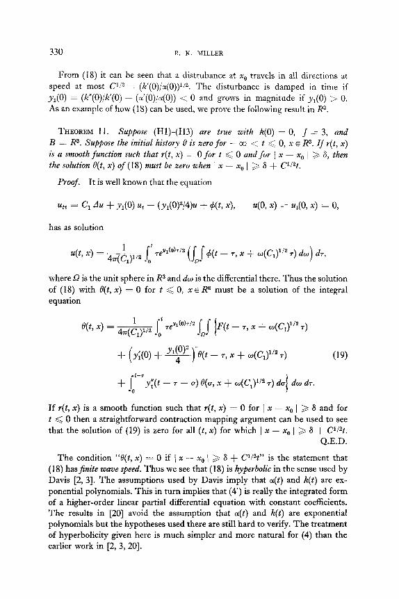
From (18) it can be seen that a distrubance at x0 travels in all directions at speed at most C1/2 =: (h’(O)/ol(O)) ljz. The disturbance is damped in time if y,(O) = (@‘(0)/k’(O) - (cL(O)/a(O)) < 0 and grows in magnitude if y,(O) :> 0. As an example of how (18) can be used, we prove the following result in R3.

THEOREM 11. Suppose (Hl)-(H3) are true with k(0) = 0, J = 3, and B = R3. Suppose the initiaE history fl is zero for -CO < t < 0, x E R3. If r(t, x) is a smooth function such that r(t, x) = 0 for t < 0 and for j x - x,, i > 6, then the solution e(t, x) of (18) must be zero when / x - x,, 1 3 S -+ CW.

Proof. It is well known that the equation

Utt = Cl Au + Yl(O) Ut - (Yl(OW4)U + $46 x), u(0, x) = u,(O, x) = 0,

has as solution

1 t ‘Ctp x) = 4T(Cl)1/2 .r

7eY1(o)7/2 iu p et - T, x + UJ(C’~)~‘~ T) dw dT, o 1

where !S is the unit sphere in R3 and dw is the differential there. Thus the solution of (18) with e(t, x) = 0 for t < 0, x E R3 must be a solution of the integral equation

1 t e(t, ‘) = 4n(C,)1i2 s

7ev1(oh/2 rsi

F(t - T, x + LU(C’~)~‘~ 7) o sa

+ (y;(o) + qqe(t - 7, x + w(cly2 T)

+ Lt-’ y;(t - 7 - u) e(u, x + u(CJ’~ T) do) dw d7.

If r(t, x) is a smooth function such that r(t, X) = 0 for / x - x0 1 > 6 and for t < 0 then a straightforward contraction mapping argument can be used to see that the solution of (19) is zero for all (t, x) for which 1 x - x0 ] > 6 + C1/2t.

Q.E.D.

The condition “Oft, X) = 0 if 1 x - x0 1 2 6 + W2t” is the statement that (18) has jinite wave speed. Thus we see that (18) is hyperbolic in the sense used by Davis [2,3]. The assumptions used by Davis imply that a(t) and k(t) are exponential polynomials. This in turn implies that (4’) is really the integrated form of a higher-order linear partial differential equation with constant coefficients. The results in [20] avoid the assumption that a(t) and R(t) are exponential polynomials but the hypotheses used there are still hard to verify. The treatment of hyperbolicity given here is much simpler and more natural for (4) than the earlier work in [2, 3, 201.


REFERENCES

1. B. D. COLEMAN AND M. E. GURTIN, Equipresense and constitutive equation for rigid heat conductors, Z. Angew. Math. Pkys. 18 (1967), 199-208.

2. P. L. DAVIS, Hyperbolic integrodifferential equations, PYOC. Amer. Math. Sot. 47 (1975), 155-160.

3. P. L. DAVIS, Hyperbolic integrodifferential equations arising in the electromagnetic theory of dialectrics, J. Dz~erential Equations 18 (197.5), 170-178.

4. P. L. DAVIS, On the Iinear theory of heat conduction for materials with memory, unpublished manuscript.

5. C. A. DESOER AND M. VIDYASAGAR, “Feedback Systems: Input-Output Properties,” Academic Press, New York, 1975.

6. J. M. FINN AND L. T. WHEELER, Wave propagation aspects of the generalized theory of heat conduction, Z. Angew. Math. Phys. 23 (1972), 927-940.

7. A. FRIED~IAN, “Partial Differential Equations of Parabolic Type,” Prentice-Hall, Englewood Cliffs, N. J., 1964.

8. A. FRIEDMAN, “Partial Differential Equations,” Holt, Rinehart & Winston, New York, 1969.

9. A. FRIEDMAN AND M. SHIMBROT, Volterra integral equations in Banach space, Trans. Amer. Math. Sot. 126 (1967), 131-179.

IO. H. GRABMUELLER, “Ueber die Loesbarkeit einer Integrodifferentialgleichung aus der Theory der Waermeleitung,” pp. 117-137, Methoden und Verfahren der Mathe- matischen Physik, Band 10, Mannheim/Wien/Zurich, Bibl. Institut, 1973.

1 I. H. GRABMUELLER, Linear Theorie der Waermeleitung in Medium mit Gedaechtnis; Existenz und Eindeutigkeit von Loesungen sum Inversen Problem, Technische Hochschule Darmstdadt, Preprint No. 226, September 1975.

12. M. E. GURTIN AND A. C. PIPKIN, A general theory of heat conduction with finite wave speeds, Arch. Rational Mech. Anal. 31 (1968), 113-126.

13. M. E. GURTIN, On the thermodynamics of materials with memory, Arch. Rational Mech. Anal. 28 (1968), 40-50.

14. J. M. HOLTZMAN, “Nonlinear System Theory: A Functional Analysis Approach,” Prentice-Hall, Englewood Cliffs, N. J., 1970.

15. S. G. KREIN, “Linear Differential Equations in Banach Space,” Translations of Mathematical Monographs 29, Amer. Math. Sot., Providence, R.I., 1971.

16. M. KREMER, “Ueber die eindeutige Loesbarkeit einer Integrodifferentialgleichungen aus der Theorie der WaermeIeitung,” Methoden und Verfahren der Mathematischen Physik, to appear.

17. R. K. MILLER, “Nonlinear Volterra Integral Equations,” Benjamin, Menlo Park, Calif., 1971.

18. R. K. MILLER, Volterra integral equations in a Banach space, FunkciaZ..Ekuac. 18 (1975), 163-193.

19. R. K. MILLER AND R. L. WHEELER, Asymptotic behavior for a linear Volterra integral equation in Hilbert space, J. Differential Equations 23 (1977), 270-284.

20. R. K. MILLER AND R. L. WHEELER, A remark on hyperbolic integrodifferential equations, J. Differential Equations 24 (1977), 51-56.

21. R. R. NACHLINGER AND L. WHEELER, A uniqueness theorem for rigid heat conductors with memory, Quart. AppZ. Math. 31 (1973), 267-273.

22. J. W. NUNZIATO, On heat conduction in materials with memory, Quart. AppZ. Math. 29 (1971). 187-204.

23. J. W. NUNZIATO, On uniqueness in the linear theory of heat conduction with finite wave speeds, SIAM J. AppZ. Math. 25 (1973), l-4.

332 H. K. MILLER

24. A. PAZY, “Semigroups of Linear Operators and Applications to Partial Differential Equations,” Lecture Notes 10, University of Maryland, College Park, Md., 1974.

25. CH.-J. DE LAVALLBE POUSSIN, “Cows d’analyse infinit&imale,” Vol. I, Gauthier- Villars, Paris, 1947.

26. R. REDHEFFER AND W. WALTER, Existence theorems for strongly coupled systems of partial differential equations over Bernstein classes, Bull. Amer. Math. Sot. 82 (1976), 899-902.

an lntegrodifferential equation for rigid heat · pdf filean lntegrodifferential equation for...

Documents