an mbo scheme on graphs for classification and image processing
TRANSCRIPT
SIAM J. IMAGING SCIENCES c© 2013 Society for Industrial and Applied MathematicsVol. 6, No. 4, pp. 1903–1930
An MBO Scheme on Graphs for Classification and Image Processing∗
Ekaterina Merkurjev†, Tijana Kostic†, and Andrea L. Bertozzi†
Abstract. In this paper we present a computationally efficient algorithm utilizing a fully or seminonlocal graphLaplacian for solving a wide range of learning problems in binary data classification and imageprocessing. In their recent work [Multiscale Model. Simul., 10 (2012), pp. 1090–1118], Bertozzi andFlenner introduced a graph-based diffuse interface model utilizing the Ginzburg–Landau functionalfor solving problems in data classification. Here, we propose an adaptation of the classic numericalMerriman–Bence–Osher (MBO) scheme for minimizing graph-based diffuse interface functionals,like those originally proposed by Bertozzi and Flenner. We also make use of fast numerical solversfor finding eigenvalues and eigenvectors of the graph Laplacian. Various computational examplesare presented to demonstrate the performance of our algorithm, which is successful on images withtexture and repetitive structure due to its nonlocal nature. The results show that our method ismultiple times more efficient than other well-known nonlocal models.
Key words. image processing, Nystrom extension, Ginzburg–Landau functional, MBO scheme
AMS subject classifications. 68U10, 49M25, 62H30, 91C20, 49-04
DOI. 10.1137/120886935
1. Introduction. This work develops a fast algorithm for a recent variational method ina graph setting. The method is inspired by diffuse interface models that have been used ina variety of problems, such as those in fluid dynamics and materials science. We considerdata represented as nodes in a weighted graph, and each edge is assigned a numerical valuedescribing the similarity between the nodes. In spectral graph theory, this approach is suc-cessfully used to perform various learning tasks in imaging and data clustering. The standardtechniques of the theory are thoroughly described in [13, 45], and the graph Laplacian, whichis discussed in more detail in section 2.2, is introduced as one of the fundamental concepts.In imaging, spectral methods are often used in image segmentation applications, as shown in[54, 33, 14].
We are particularly interested in nonlocal total variation methods, as they are a link be-tween spectral graph theory and diffuse interface models and thus can be used as a motivationfor our algorithm. These methods are used in numerous image processing applications. Theywere initially developed as methods for image denoising [9, 29] but were successfully appliedto many other image processing problems such as inpainting and reconstruction in [30, 63, 49],image deblurring in [40], and manifold processing in [18].
Bertozzi and Flenner introduce a graph-based model based on the Ginzburg–Landau func-
∗Received by the editors August 3, 2012; accepted for publication (in revised form) May 30, 2013; publishedelectronically October 10, 2013. This work was supported by ONR grants N000141210040 and N00014120838,AFOSR MURI grant FA9550-10-1-0569, and by the W. M. Keck Foundation.
http://www.siam.org/journals/siims/6-4/88693.html†Mathematics Department, UCLA, Los Angeles, CA 90095-1555 ([email protected], [email protected].
edu, [email protected]). The first author was also supported by an NSF graduate fellowship.
1903
1904 EKATERINA MERKURJEV, TIJANA KOSTIC, AND ANDREA L. BERTOZZI
tional in their work [8]. To define the functional on a graph, the spatial gradient is replacedby a more general graph gradient operator. Bertozzi and Flenner propose a classificationalgorithm by minimizing the Ginzburg–Landau functional with a fidelity term,
(1.1) E(u) =ε
2
∫|∇u|2dx+
1
ε
∫W (u)dx+ F (u, u0),
where u0 is the initial state of the system. They replace the ε2
∫ | � u|2dx term with a moregeneral graph operator term, εu ·Lsu, to be discussed in detail in sections 2.2 and 2.3, so that
(1.2) E(u) = εu · Lsu+1
ε
∫W (u)dx+
∫F (u, u0).
The functional is minimized using the method of gradient descent, resulting in the followingexpression:
(1.3)∂u
∂t= −εLsu− 1
εW ′(u)− ∂F
∂u.
Note that this is just the Allen–Cahn equation with a fidelity term, where Δu is replaced bya graph operator term −Ls. Properties of the operator Ls will be explained in more detail insections 2.2 and 2.3. Taking F to be 1
2Cλ(x)(u− u0)2 for some constant C, one obtains
(1.4)∂u
∂t= −εLsu− 1
εW ′(u)−Cλ(x)(u− u0).
The main purpose of this paper is to develop a fast and simple method for solving (1.4) in thesmall ε limit. To achieve our goal, we created a graph-based MBO (Merriman–Bence–Osher)scheme. The famous MBO scheme uses simple threshold dynamics to approximate motionby mean curvature. Since the Allen–Cahn equation is closely related to motion by meancurvature, the MBO scheme has been proven to be a very successful tool in solving differentvariants of the Allen–Cahn equation. For example, the authors of [22] propose an adaptationof the MBO scheme to minimize the piecewise constant Mumford–Shah functional. Inspiredby the efficiency and the robustness of the MBO scheme, we decide to adapt it solve (1.4).However, the implementation of the proposed scheme poses many computational challenges.The quadratic size of the graph Laplacian could make the iterative process of our algorithmvery computationally expensive. To reduce the dimension of the graph Laplacian and makethe computation more efficient, the authors of [8] propose the Nystrom extension method[25] for approximating eigenvalues and the corresponding eigenvectors of the graph Laplacian.To maximize the performance of our algorithm, for each data set we use either the Nystromextension or the Raleigh–Chebyshev algorithm proposed in [1]. The details of our algorithmare discussed in section 3, after sections 2.2–2.4 on the relevant background.
There are several reasons for the efficiency of our algorithm. Our method is a geometricapproach to the minimization problem, as opposed to the more traditional L1 minimizationapproach. In addition, our method is more simple and less computationally complex thanthat described in the paper of Bertozzi and Flenner [8]. Moreover, we take advantage offast numerical solvers for eigenvalue/eigenvector decomposition as well as using only a smallnumber of principal components in our numerical iterations.
AN MBO SCHEME ON GRAPHS 1905
In this paper, we go beyond the applications presented in [8] and devise a nonlocal in-painting algorithm. To show the efficiency of our algorithm, we compare the computationaltimes of our algorithm against those obtained by the state-of-the-art nonlocal inpainting al-gorithm form [30]. For the data classification problem presented in Figure 2, the comparisonof our results to those obtained in the new work [8] demonstrate that our algorithm producesa significant speedup, while producing comparable results in terms of quality. In section 4,the inpainting results show that our method is about five times more efficient than otherwell-known nonlocal models, while being comparable in quality.
This paper is organized as follows. In section 1, we review the motivation for our method aswell as some relevant background such as diffuse interfaces, the Ginzburg–Landau functional,graphs, nonlocal operators, and the MBO scheme. We then introduce our algorithm, whichis applied to classification and inpainting in sections 2 and 3, respectively; show results; andinclude comparisons to some of the recent methods. The performance of our data classificationalgorithm is compared against the algorithm from [8]. The algorithm from [8] is more accuratethan other standard classification algorithms, such as a naive Bayes decision trees from [50]and p-Laplacian spectral clustering from [56]. We compared our inpainting results to thoseobtained using the split Bregman method from [62], which is a well-known efficient algorithmfor nonlocal TV minimization. The advantage of this new method is its speed and its abilityto recover texture and repetitive structure in an image.
2. Background. In this section, we present some useful background information. In sec-tion 2.1, we review the Ginzburg–Landau functional, which is the core of the model of Bertozziand Flenner in [8]. Our algorithm is graph-based, so a background on graphs is given in sec-tion 2.2. To understand the motivation behind the definition of the graph Laplacian, one mayturn to the theory of nonlocal operators, outlined in section 2.3. The MBO scheme, whichserves as the core element in our model, is described in section 2.4. Finally, two methods tocompute eigenvalues and associated eigenvectors are described in section 2.6.
2.1. Ginzburg–Landau functional. Numerous image segmentation energy functionals usea binary segmentation function that takes a certain value inside the segmented region and adifferent one outside of the segmented region. In their pioneering work [46], Mumford andShah propose an energy functional that uses the perimeter of the segmentation function as aregularizer. Many papers, such as [12], successfully use the total variation (TV) semi norm
(2.1) ||u||TV =
∫Ω|∇u|dx
to approximate the perimeter of the front between the two values of the segmentation function.As an alternative to this approach, some researchers, such as Esedoglu and Tsai in their work[22], use the Ginzburg–Landau functional
(2.2) GL(u) =ε
2
∫|∇u|2dx+
1
ε
∫W (u)dx
to approximate the perimeter of the front. W (u) is a double well potential. In this work,W (u) = (u2−1)2 is used. Note that, due to the nature of the potential, the functional is usedfor binary data.

1906 EKATERINA MERKURJEV, TIJANA KOSTIC, AND ANDREA L. BERTOZZI
A proof in [39] shows that the perimeter is the limit in the sense of Γ-convergence of theGinzburg–Landau functional. Therefore, one can write
(2.3) GL(u)→Γ C|u|TV .
This convergence allows the two functionals to be interchanged in some cases. One mightprefer to use the Ginzburg–Landau functional instead of the TV seminorm since its highestorder term is purely quadratic, which allows for efficient minimization procedures. In contrast,minimization of the TV seminorm leads to a nonlinear curvature term, making it less trivialto solve numerically. However, recent advances, such as the split Bregman method describedin [31], have made progress in such problems.
Due to its connection to the TV seminorm, the Ginzburg–Landau functional has also oftenbeen used in image processing and in various image processing applications, such as inpainting[16, 7] and segmentation [19, 22]. In practice, one would minimize
(2.4) E(u) = GL(u) + F (u, u0),
where F is the fidelity term and u0 is the initial state of the system. In the case of inpainting,the fidelity term is C
∫(u − u0)
2, where one integrates over the known region only. Fordenoising, the term is an L2 fit, C
∫(u−u0)
2. In the case of deblurring, it is C∫(K ∗u−u0)
2,where K is some kernel. Of course, a different norm, such as the L1 norm, can be used.
When one minimizes the Ginzburg–Landau functional, the function u approaches eitherone of the two minimizers, 1 and −1, of the double well potential. However, the presenceof the gradient term will force u to be somewhat smooth, i.e., without any sharp transitionsbetween 1 and −1. Therefore, the function that minimizes the functional will have regionswhere it is close to −1, regions close to 1, and a thin region of scale O(ε) where it is somewherein between. Since the minimizer appears to have two phases with an interface between them,models involving the Ginzburg–Landau functional are typically referred to as “diffuse interfacemodels.”
2.2. Background on graphs. In this paper, to create a nonlocal method, we use thetheory of graphs, described in [13]. Consider an undirected graph G = (V,E), where V andE are the sets of vertices and edges, respectively. In the tests done in this paper, the verticesare, for example, points in R
n or pixels in an image. Let w be the weight function, wherew(i, j) represents the weight (often measured between 0 and 1) between vertices i and j andw(i, i) is set to zero. The weight represents a measure of similarity between the vertices; thus,two vertices having a weight close to 1 are very similar to each other, and two vertices havinga weight close to 0 are dissimilar.
Now let the degree of a vertex i ∈ V be defined as
(2.5) d(i) =∑j∈V
w(i, j).
Using the above, one defines the graph Laplacian to be the matrix L such that
L(i, j) =
{d(i) if i = j,
−w(i, j) otherwise.
AN MBO SCHEME ON GRAPHS 1907
If we define the degree matrix D to be the N ×N diagonal matrix with diagonal elementsd(i), then the graph Laplacian can be written in matrix form as L = D−W , where W is thematrix w(i, j). The matrix W is sometimes referred to as the “affinity matrix.”
Note that the graph Laplacian satisfies the equations
(2.6) Lu(i) =∑j
w(i, j)(u(i) − u(j)),
(2.7) u · Lu =1
2
∑i,j
w(i, j)(u(i) − u(j))2
for all u ∈ Rn and has nonnegative, real-valued eigenvalues, including 0.
When working with the graph Laplacian, one must consider the behavior that arises asthe sample size grows larger. Increasing sample size leads to decreasing grid size; thus, theoperator must be scaled to converge to the differential Laplacian as N → ∞, where N isthe number of vertices. Although several versions that have been shown to have the correctscaling in the limit exist, the one used in this paper is the symmetric Laplacian
(2.8) Ls = D− 12LD− 1
2 = I −D− 12WD− 1
2
that satisfies
(2.9) u · Lsu =1
2
∑i,j
w(i, j)(u(i) − u(j))2√d(i)d(j)
∀u ∈ Rn.
We use this version since the symmetric property of the matrix allows for more efficientalgorithms for calculating eigenvectors, which is necessary for our algorithm.
Another version that is commonly used is the random walk Laplacian,
(2.10) Lw = D−1L = I −D−1W,
which is related to Markov processes. More detail about normalized Laplacians is given in[13] and [59].
2.2.1. Choice of similarity function. As mentioned in previous sections, the weight func-tion w(i, j) is a function that measures the degree of similarity between vertices i and j.Therefore, it is necessary to choose the function in such a way that two vertices that areheavily weighted by w, i.e., w(i, j) large, are also closely related in the data. Although severaloptions for w are discussed in [59], the choice depends on the problem, so no general theorycan be formulated.
One popular choice for the similarity function is the Gaussian function
(2.11) w(i, j) = e−d(i,j)2
σ2 ,
where D(i, j) is some distance measure between the two vertices i and j, and σ is a parameterto be chosen. Von Luxburg in [59] explains that σ can be chosen to be on the order of
1908 EKATERINA MERKURJEV, TIJANA KOSTIC, AND ANDREA L. BERTOZZI
log(n)+1, where n is the number of vertices. This similarity function is an appropriate choicewhen vertices are, for example, points in R
n, since two points that are close together are morelikely to belong to the same cluster than are two points that are far apart.
Another choice for the similarity function used in this work is the Zelnik-Manor and Peronaweight function for sparse matrices described in [61]:
(2.12) w(i, j) = e− d(i,j)2√
τ(i)τ(j) ,
where the local parameter√
τ(i) = d(i, k) and k is the Mth closest vertex to vertex i. Asnoted in [8], one should use this similarity function for classification when there exist multiplescales to be classified. In [61], M is chosen to be 7, while in [56], it is 10. Depending on thedata set, we use either (2.11) or (2.12).
The choice of d(i, j) varies with the data set. If one wants to cluster points in Rn, a
reasonable choice for d(i, j) is the Euclidean distance between points i and j. In the case ofimage processing, where the vertices are the pixels in the image, to construct d(i, j), we usethe concept of feature vectors, as in [8]. Each vertex i is assigned an n-dimensional featurevector, and d(i, j) is then the weighted 2-norm (where each coordinate of the vector is assigneda weight) of the difference of the feature vectors of pixels i and j. More details on d(i, j) inthis case are given in sections 4.1 and 4.2.
2.2.2. Graph clustering and the graph Laplacian. The theory shown below justifies theuse of the (thresholded) second eigenvector of Ls as an initialization when applying our clas-sification algorithm to the two-moons data set, which will be described in section 3.1.1.
The goal of graph clustering is to partition the graph so that the weights between verticesof different groups are small and the weights between vertices within the same group are large.In this section, we deal with a binary problem only. A mincut approach to the above problemis to partition a set of vertices V into sets A and A in such a way that
(2.13) cut(A, A) =∑
x∈A,y∈Aw(x, y)
is minimized. This mincut problem can be solved using an efficient algorithm like the ones in[55, 37, 38].
However, this problem leads to poor classification in many cases since the resulting “bad”partition often isolates one vertex from the rest of the set [44]. One way to overcome thisproblem is to use correct normalization, i.e., to force the sets A and A to be “large.” Let
(2.14) vol(A) =∑x∈A
d(x).
Then the modified problem is to find a subset A of V such that
(2.15) Ncut(A, A) =cut(A, A)
vol(A)+
cut(A, A)
vol(A)
is minimized. This is a NP-hard discrete problem [60]. One way to simplify it would be toallow the solution to take arbitrary values in R. This leads to the following relaxed Ncut
AN MBO SCHEME ON GRAPHS 1909
problem:
(2.16) minA⊂Y〈u,Lsu〉, u ⊥ D
121, ||u||2 = vol(Y ).
The fact that the above problem obtains a real-valued solution instead of a discrete-valuedsolution, like problem (2.15), is emphasized.
The relaxed problem (2.16) has been applied to many segmentation problems; for example,appealing results are shown in [54]. To solve the above problem, one can apply the Raleigh–Ritz theorem, and the solution is given by the second eigenvector of the symmetric graphLaplacian Ls [59].
2.3. Nonlocal operators. In general, image processing methods that are local fail toproduce satisfactory results on images with repetitive structures and textures because theyoperate only on small neighborhoods, without using any information about the whole domain.The advantage of nonlocal operators is that they contain data about the whole vertex set andare thus more successful with those types of images.
Zhou and Scholkopf in their papers [67, 64, 66, 65] formulated a theory of nonlocal oper-ators that is related to the discrete graph Laplacian described in section 2.2. Buades, Coll,and Morel applied this nonlocal theory to denoising algorithms in their work [9]. Gilboa andOsher proposed using nonlocal operators to define functionals involving the TV seminorm forvarious image processing applications in their work [29].
We review nonlocal calculus below, where all definitions are continuous. Let Ω ∈ Rn, u(x)
be a function u : Ω→ R, and the nonlocal derivative be defined as
(2.17)∂u
∂y(x) =
u(y)− u(x)
d(x, y), x, y ∈ Ω,
where d is some positive distance defined on the space and 0 < d(x, y) ≤ ∞ for all x, y. If the(symmetric) weight function is defined as
(2.18) w(x, y) =1
d(x, y)2,
the nonlocal derivative can be written as
(2.19)∂u
∂y(x) = (u(y)− u(x))
√w(x, y).
We now consider vectors and denote them by �v = v(x, y) ∈ Ω×Ω. Let �v1 and �v2 be two suchvectors. We define the dot product and the inner product as
(2.20) (�v1 · �v2)(x) =∫Ωv1(x, y)v2(x, y)dy,
(2.21) 〈�v1, �v2〉 = 〈�v1 · �v2, 1〉 =∫Ω×Ω
v1(x, y)v2(x, y)dxdy.
1910 EKATERINA MERKURJEV, TIJANA KOSTIC, AND ANDREA L. BERTOZZI
The magnitude of a vector can be defined as
(2.22) |v|(x) =√�v · �v =
√∫Ωv(x, y)2dy,
while the nonlocal gradient �wu(x) : Ω→ Ω× Ω is the vector of all partial derivatives:
(2.23) (∇wu)(x, y) = (u(y)− u(x))√
w(x, y), x, y ∈ Ω.
With the above definitions, the nonlocal divergence divw�v(x) : Ω × Ω → Ω is defined asthe adjoint of the nonlocal gradient:
(2.24)(divw
�v)(x) =
∫Ω(v(x, y) − v(y, x))
√w(x, y)dy.
The Laplacian is now defined as
(2.25) Δwu(x) =1
2divw(∇wu(x)) =
∫Ω(u(y)− u(x))w(x, y)dy.
Since the graph Laplacian was defined in section 2.2 as
(2.26) Lu(x) =∑y
w(x, y)(u(x) − u(y)),
one can interpret −Lu(x) as a discrete approximation of Δwu. Note that a constant of 12 was
needed here to relate the two Laplacians.According to the nonlocal calculus described above,
(2.27)
∫Ω|∇u|2dx =
∫Ω×Ω
(u(y)− u(x))2w(x, y)dxdy.
Since
(2.28) u · Lu =1
2
∑x,y
w(x, y)(u(x) − u(y))2,
one can consider 2u · Lu to be the discrete graph version of∫ |∇u|2dx.
In their paper [8], Bertozzi and Flenner replace the ε2
∫ |∇u|2dx term of (2.2) by εu ·Lu(x).However, normalization of the Laplacian is necessary (refer to the beginning of section 2.2 orto [8]), so instead they use
(2.29) εu · Lsu =ε
2
∑x,y
w(x, y)(u(x) − u(y))2√d(x)d(y)
.
When the variational solution u takes the values −1 or 1,
(2.30) u ·Lsu = C +4∑
x∈A,y∈A
w(x, y)√d(x)d(y)
− 2
⎛⎝ ∑
x∈A,y∈A
w(x, y)√d(x)d(y)
+∑
x∈A,y∈A
w(x, y)√d(x)d(y)
⎞⎠ .
AN MBO SCHEME ON GRAPHS 1911
In this case, C is a constant that varies with the graph but not with the partition. The rep-resentation shows that the above is minimized when the normalized weights between verticesof different groups are small but the normalized weights between vertices within a group arelarge. This is precisely the goal of graph clustering. Therefore, by replacing the ε
2
∫ | � u|2dxterm of (2.2) with εu ·Lsu, thus creating a graph-based version of (2.2), and then minimizingthe resulting equation, one achieves the desired segmentation.
The Γ-convergence of the graph-based Ginzburg–Landau functional is investigated in [57].The authors prove that as ε→ 0, the limit is related to the TV seminorm and cut from (2.13).
Another important operator that arises from the need to define variational methods ongraphs is the mean curvature on graphs. This nonlocal operator was introduced by Osher andShen in [48], who defined it via graph-based p-Laplacian operators. p-Laplacian operators area family of quasi-linear elliptic partial differential operators defined for 1 ≤ p <∞:
(2.31) Lp(f) = ∇ · (| ∇f |p−2 ∇f).In the special case p = 2, the p-Laplacian is just a regular Laplacian. For p = 1, the p-Laplacian represents curvature.
The discrete graph version of p-Laplace operators is defined in [18] as
(2.32) Lp(u(x)) =1
p
∑(x,y)∈E
w(x, y)(‖∇u(x)‖p−2 + ‖∇u(y)‖p−2)(u(x)− u(y)).
Note that the graph 2-Laplacian is just the graph Laplacian, which is consistent with thecontinuous case.
Let us now define the mean curvature on graphs—the discrete analogue of the meancurvature of the level curve of a function defined on a continuous domain of RN :
(2.33) κw =1
2
∑(x,y)∈E
w(x, y)
(1
‖∇u(x)‖ +1
‖∇u(y)‖)(u(x)− u(y)).
Note that in the case of an unweighted mesh graph, κw becomes a numerical discretizationof the mean curvature. This curvature, κw, is also used in [15] as a regularizer in a graphadaptation of the Chan–Vese method. In their work-in-progress [58], van Gennip et al. proposea different definition of mean curvature on graphs and prove convergence of the MBO schemeon graphs.
2.4. Review of the MBO scheme. The idea of approximating mean curvature flow usingthreshold dynamics was introduced in [43] by Merriman, Bence, and Osher. To explain theintuition behind the numerical scheme they propose, the authors analyze the mean curvatureflow of the curve C = ∂Σ using diffusion of the characteristic function χ of the set Σ. Ifone imagines an interface, such as χ, and then applies the heat equation χt = Δχ, then thediffusion blunts the sharp points on the front but has little impact on the flatter parts, thusleaving the χ = 1
2 level set invariant to diffusion. By changing the coordinates to polar form,the authors of [43] show that the 1
2 -level set also moves according to some curvature dependentmotion. Therefore, if one diffuses the characteristic function of a set with boundary C for ashort time and then identifies the boundary of the “new set” with the 1
2 -level set, the curve C
1912 EKATERINA MERKURJEV, TIJANA KOSTIC, AND ANDREA L. BERTOZZI
moves with a normal velocity that is at any given point equal to the mean curvature at thatpoint. The above analysis is local, so the timestep needs to be short enough so that it is validbut long enough so that the curve is moving.
From the previous discussion follows the MBO numerical scheme for approximation of themotion of u by mean curvature at discrete times:
• Step 1 (diffusion). Let v(x) = S(δt)un(x), where S(δt) is the propagator (by time δt) of
(2.34)∂v
∂t= Δv.
• Step 2 (thresholding). Set
un+1(x) =
{1 if v(x) ≥ 1
2 ,
0 if v(x) < 12 .
2.5. Applications of the MBO scheme. We are interested in motion by mean curvaturebecause it is closely related to the Ginzburg–Landau functional, which we use here as aregularizer. The gradient descent of the Ginzburg–Landau functional yields the Allen–Cahnequation:
(2.35)∂u
∂t= 2εΔu− 1
εW ′(u).
Here W is the double well potential W (u) = (u2 − 1)2. It is proven in [51] that as ε → 0+,the rescaled solutions uε(x, t/ε) of the above equation move according to mean curvatureof the interface between the −1 and 1 phases of the solutions. In addition, [3] and [23]present rigorous proofs that the MBO algorithm approximates motion by mean curvature.This implies that for the small values of ε, the MBO thresholding scheme can be used tonumerically solve the Allen–Cahn equation.
Multiple extensions, adaptations, and applications of the MBO scheme are present inliterature. We find the modification of the MBO scheme for solving the inhomogeneous Allen–Cahn equation proposed in [22] particularly interesting. To create a fast image segmentationalgorithm, Esedoglu and Tsai propose a thresholding scheme for minimizing a diffuse interfaceversion of the piecewise constant Mumford–Shah functional,
(2.36) MSε(u, c1, c2) =
∫Dε|∇u|2 + 1
εW (u) + λ{u2(c1 − f)2 + (1− u)2(c2 − f)2}dx,
where f is the image. The first variation of the model (2.36) yields the following gradientdescent equation:
(2.37) ut = 2εΔu− 1
εW ′(u) + 2λ{u(c1 − f)2 + (1− u)(c2 − f)2},
and the adaptation of the MBO scheme is used to solve it. Esedoglu and Tsai propose thefollowing scheme (similar to the MBO scheme, where the propagation step based on the heatequation is combined with thresholding):

AN MBO SCHEME ON GRAPHS 1913
• Step 1. Let v(x) = S(δt)un(x), where S(δt) is a propagator by time δt of the equation
wt = Δw − 2λ(w(c1 − f)2 + (1− w)(c2 − f)2
)with appropriate boundary conditions.
• Step 2. Set
un+1(x) =
{0 if v(x) ∈ (−∞, 12 ],1 if v(x) ∈ (12 ,∞).
We also use an adaptation of the MBO scheme to solve our equation (1.4), but the mostimportant difference between our method and the above approach, besides a different energyto minimize, is that we generalize to graphs.
Some other extensions of the MBO scheme appeared in [20, 21, 42]. An efficient algorithmfor motion by mean curvature using adaptive grids was proposed in [52].
2.6. Computation of eigenvectors. Our method involves the computation of eigenvaluesand associated eigenvectors of the symmetric graph Laplacian. In practice, one needs tocompute only a fraction of the eigenvalues and eigenvectors (since eigenvectors with verysmall eigenvalues are not very significant computationally), and different methods of doing soare used depending on the size of the domain.
When the graph is sparse and is of moderate size, around 5000 × 5000 or less, we usea Rayleigh–Chebyshev procedure outlined in [1]. It is a modification of an inverse subspaceiteration method that uses adaptively determined Chebyshev polynomials. The procedureis also a robust method that converges rapidly and that can handle cases when there areeigenvalues of multiplicity greater than one.
When the graph is very large, such as in the case of image classification, the Nystromextension method, to be described in the next section, is used.
2.6.1. Nystrom extension for fully connected graphs. Nystrom extension [8, 26, 25, 4]is a matrix completion method often used in image processing applications, such as kernelprinciple component analysis [17] and spectral clustering [47]. This procedure performs muchfaster than many alternate techniques because it uses approximations based on calculationson small submatrices of the original large matrix. When the size of the matrix becomes verylarge, this method is especially valuable.
Note that if λ is an eigenvalue of W = D− 12WD− 1
2 , then 1 − λ is an eigenvalue of Ls,and the two matrices have the same eigenvectors. We formulate a method to calculate theeigenvectors and eigenvalues of W and thus of Ls.
Let w be the similarity function, λ be an eigenvalue of W , and φ its associated eigenvector.The Nystrom method approximates the eigenvalue equation
(2.38)
∫Ωw(y, x)φ(x)dx = λφ(x)
using a quadrature rule, a technique to find weights cj(y), and a set of L interpolation pointsX = {xj} such that
(2.39)L∑
j=1
cj(y)φ(xj) =
∫Ωw(y, x)φ(x)dx + E(y),
1914 EKATERINA MERKURJEV, TIJANA KOSTIC, AND ANDREA L. BERTOZZI
where E(y) represents the error in the approximation.We use cj(y) = w(y, xj) and choose the L interpolation points randomly from the vertex
set V . Denote the set of L randomly chosen points by X = {xi}Li=1 and its complement byY . Partitioning Z into Z = X ∪ Y and letting φk(x) be the the kth eigenvector of W and λk
its associated eigenvalue, we obtain the system of equations
(2.40)∑xj∈X
w(yi, xj)φk(xj) = λkφk(yi) ∀yi ∈ Y, ∀k ∈ 1, . . . , L.
This system of equations cannot be solved directly, since the eigenvectors are not known. Toovercome this problem, the L eigenvectors of W are approximated using calculations involvingsubmatrices of W .
Let WXY be defined as ⎡⎢⎣
w(x1, y1) . . . w(x1, yN−L)...
. . ....
w(xL, y1) . . . w(xL, yN−L)
⎤⎥⎦ ,
where W has dimension N×N . The matrices WY X , WXX , and WY Y can be defined similarly.Notice that WXY = WY X
T . Then the matrix W can be written as[WXX WXY
WY X WY Y
].
To calculate the eigenvalues and eigenvectors of W , one must correctly normalize the aboveweight matrix. The correct normalization is achieved by the following calculations, where wedenote by 1K the K-dimensional unit vector.
Let the matrices dX and dY be defined as
dX = WXX1L +WXY 1N−L,
dY = WY X1L + (WY XW−1XXWXY )1N−L.
(2.41)
If A./B denotes componentwise division between matrices A and B, and vT denotes thetranspose of vector v, then define the matrices WXX and WXY as
WXX = WXX ./(sXsTX),
WXY = WXY ./(sXsYX),(2.42)
where sX =√dX and sY =
√dY .
It is shown in [8] that if WXX = BXDBTX , and if A and Γ are matrices such that
(2.43) ATΓA = WXX + W− 1
2XXWXY WY XW
− 12
XX ,
then the eigenvector matrix V consisting of L eigenvectors of W and thus of Ls is given by[BXD
12BT
XAΓ− 12
WY XBXD− 12BT
XAΓ− 12
],

AN MBO SCHEME ON GRAPHS 1915
while I − Γ contains the corresponding eigenvalues of Ls in its diagonal entries.Therefore, the efficiency of the Nystrom extension method lies with the fact that when
computing the eigenvalues and eigenvectors of an N ×N matrix, where N is large, it approx-imates them using calculations involving only much smaller matrices, the largest of which hasdimension N × L, where L is small.
Although this method is very efficient, there are problems when it is applied to binaryimage inpainting, especially when the image has a repetitive structure. This occurs becauseof singular or nearly singular matrices that arise in the calculations of the Nystrom extensionmethod. Therefore, in this case, we use the Rayleigh–Chebyshev procedure of [1] to calculatethe eigenvalues and associated eigenvectors.
3. Classification algorithm. We construct a new classification algorithm by proposing adifferent approach to minimizing (1.2) than that in [8] to obtain a more simple and efficientmethod that eliminates the diffuse interface parameter ε. Our scheme is based on a variationof the MBO scheme.
As was shown in section 2.4, for small ε, the MBO thresholding scheme can be used toevolve the Allen–Cahn equation to steady state. The scheme consists of two steps: a heatequation propagation step and a thresholding step.
A candidate for the threshold dynamics of (1.2) is found by splitting (1.4), which is theAllen–Cahn equation plus an extra fidelity term. There are several options, including splittingthe equation into three steps, but we choose the possibility in which (1.4) is split so that thethresholding step resembles the one in the original MBO scheme, as is done in [22] andexplained in section 2.5.
Therefore, our algorithm consists of alternating between the following two steps to obtainapproximate solutions un(x) at discrete times:• Step 1 (heat equation with forcing term). Propagate using
(3.1)∂y
∂t= −Lsy − C1λ(x)(y − u0),
starting with un. Note that C1 can be different from the original C.• Step 2 (thresholding). Set
un+1(x) =
{1 if y(x) ≥ 0,
−1 if y(x) < 0.
Note that we now use 0 as the thresholding value (instead of 12 as in the original MBO
scheme), since the values of u are concentrated at −1 and 1, not 0 and 1.We have decided to discretize (3.1) above in the following manner:
(3.2)un+1 − un
dt= −Lsu
n+1 − C1λ(x)(un − u0).
Note that the symmetric Laplacian is calculated implicitly. This is due to the stiffness of theoperator, which is caused by a wide range of its eigenvalues. An implicit term is needed, sincean explicit scheme requires that all the scales of the eigenvalues be resolved numerically. The

1916 EKATERINA MERKURJEV, TIJANA KOSTIC, AND ANDREA L. BERTOZZI
above scheme is used because it is the simplest scheme possible keeping the Laplacian termimplicit.
The scheme is solved using the spectral decomposition of the symmetric graph Laplacian.Let un =
∑k a
nkφk(x) and C1λ(u
n − u0) =∑
k dnkφk(x), where φ(x) are the eigenfunctions of
the symmetric Laplacian. Using the obtained representations and (3.2), we obtain
(3.3) an+1k =
ank − dtdnk1 + dtλk
,
where λk are the eigenvalues of the symmetric graph Laplacian.
This spectral decomposition method is chosen because it is very efficient. Without it,the discrete Laplacian term by itself requires O(N2) calculations (without assuming any spar-sity). However, when using spectral decomposition, we obtain the advantage of only having tocalculate the first few largest eigenvalues and associated eigenvectors (as the smallest eigenval-ues and associated eigenvectors become insignificant in calculations). Therefore, the discreteLaplacian term now requires only O(NL) calculations, where L is the number of eigenval-ues/eigenvectors calculated. In our data sets, L � N . Of course, this method is useful onlyif there is an efficient way to calculate the eigenvalues and eigenvectors of the symmetricLaplacian. For the results in this paper, we use two methods, described in section 2.6.
Therefore, the new algorithm consists of the following:
• Step 1. Create a graph from the data, choose a similarity function, and then calculatethe symmetric graph Laplacian.
• Step 2. Calculate the eigenvectors and eigenvalues of the symmetric graph Laplacian.It is necessary only to calculate a portion of the eigenvectors.
• Step 3. Initialize u.
• Step 4. Apply the two-step scheme (to minimize the Ginzburg–Landau functional)described above for a certain number of iterations until a stopping criterion is satisfied. Usethe following method:
1. Let a0k =∑
x u0(x)φk(x) and d0k(x) = 0 for all x.
2. Until a stopping criterion is satisfied, do the following:
a. Repeat for some number s of steps:
1. ank ←ank−δtdnk1+δtλk
,
2. y(x) =∑
k ankφk(x),
3. dnk =∑
xC1(y − u0)(x)φk(x).
b. (thresholding part)
un+1(x) =
{1 if y > 0,
−1 otherwise.
c. Let an+1k =
∑x un+1(x)φk(x) and dn+1
k =∑
xC1(y − u0)(x)φk(x).
The parameter δt is chosen using trial and error. The stopping criteria we use in our work
is||unew−uold||22
||unew||22< α = 0.0000001.
AN MBO SCHEME ON GRAPHS 1917
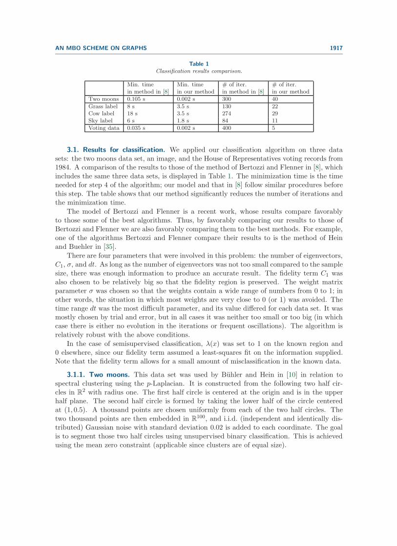
Table 1Classification results comparison.
Min. time Min. time # of iter. # of iter.in method in [8] in our method in method in [8] in our method
Two moons 0.105 s 0.002 s 300 40
Grass label 8 s 3.5 s 130 22Cow label 18 s 3.5 s 274 29Sky label 6 s 1.8 s 84 11
Voting data 0.035 s 0.002 s 400 5
3.1. Results for classification. We applied our classification algorithm on three datasets: the two moons data set, an image, and the House of Representatives voting records from1984. A comparison of the results to those of the method of Bertozzi and Flenner in [8], whichincludes the same three data sets, is displayed in Table 1. The minimization time is the timeneeded for step 4 of the algorithm; our model and that in [8] follow similar procedures beforethis step. The table shows that our method significantly reduces the number of iterations andthe minimization time.
The model of Bertozzi and Flenner is a recent work, whose results compare favorablyto those some of the best algorithms. Thus, by favorably comparing our results to those ofBertozzi and Flenner we are also favorably comparing them to the best methods. For example,one of the algorithms Bertozzi and Flenner compare their results to is the method of Heinand Buehler in [35].
There are four parameters that were involved in this problem: the number of eigenvectors,C1, σ, and dt. As long as the number of eigenvectors was not too small compared to the samplesize, there was enough information to produce an accurate result. The fidelity term C1 wasalso chosen to be relatively big so that the fidelity region is preserved. The weight matrixparameter σ was chosen so that the weights contain a wide range of numbers from 0 to 1; inother words, the situation in which most weights are very close to 0 (or 1) was avoided. Thetime range dt was the most difficult parameter, and its value differed for each data set. It wasmostly chosen by trial and error, but in all cases it was neither too small or too big (in whichcase there is either no evolution in the iterations or frequent oscillations). The algorithm isrelatively robust with the above conditions.
In the case of semisupervised classification, λ(x) was set to 1 on the known region and0 elsewhere, since our fidelity term assumed a least-squares fit on the information supplied.Note that the fidelity term allows for a small amount of misclassification in the known data.
3.1.1. Two moons. This data set was used by Buhler and Hein in [10] in relation tospectral clustering using the p-Laplacian. It is constructed from the following two half cir-cles in R
2 with radius one. The first half circle is centered at the origin and is in the upperhalf plane. The second half circle is formed by taking the lower half of the circle centeredat (1, 0.5). A thousand points are chosen uniformly from each of the two half circles. Thetwo thousand points are then embedded in R
100, and i.i.d. (independent and identically dis-tributed) Gaussian noise with standard deviation 0.02 is added to each coordinate. The goalis to segment those two half circles using unsupervised binary classification. This is achievedusing the mean zero constraint (applicable since clusters are of equal size).

1918 EKATERINA MERKURJEV, TIJANA KOSTIC, AND ANDREA L. BERTOZZI
An affinity matrix W is created using the weight function w(i, j) = e− d(i,j)2√
(τ(i)τ(j)) , a weightfunction introduced by Zelnik-Manor and Perona in [61], where τ(i) is the Euclidean distancebetween point i and the Mth closest point to it, and d(i, j) is the Euclidean distance betweenpoints i and j. The matrix W (i, j) is made sparse by setting W (i, j) equal to zero if point j isnot among the Mth closest points to point i. It is then “symmetrized” by setting W (i, j) =max(W (i, j),W (j, i)).
To calculate the eigenvectors, the Rayleigh–Chebyshev procedure [1] is used, since thegraph is not large and Nystrom extension is inefficient for sparse graphs [8].
Since the problem is unsupervised binary classification (and thus no prior knowledge ofclass membership is assumed for any of the points), in Step 4 of the algorithm, there is nofidelity term, so λ(x) = 0 for all x. Thus, dnk = 0 for all k and n. However, since the goal isto achieve two clusters of equal size, we can use the mean zero constraint. This results in twoclasses of the same size. Due to the mean zero constraint,
∫u(x)dx = 0, before thresholding,
one applies the mean constraint to y by subtracting its mean from each element of y. Forinitialization of u, we use the sign of the second eigenvector of the symmetric Laplacian afterthe mean zero constraint has been applied to it. The use of such initialization was justified insection 2.2.2.
We compared our results to the method of Bertozzi and Flenner in [8] by running simula-tions on 35 different randomly generated two moons data sets, each taking around 2 secondsto run. The average accuracy was 96.0520% and 96.0460% for our method and the method in[8], respectively. However, 40 iterations in the minimization procedure were used, compared to300 needed using the method in [8]. Therefore, our method resulted in a significant decreasein the number of iterations. The minimization time was also decreased from 0.105 seconds to0.002 seconds. These results are displayed in Table 1.
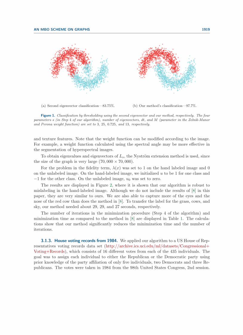
We also compared our results to a spectral clustering method of thresholding the secondeigenvector of Ls. The results are displayed in Figure 1. Clearly, clustering using the secondeigenvector does not result in an accurate binary classification.
3.1.2. Semisupervised image labeling. We also applied our algorithm to segmenting ob-jects in images of cows from the Microsoft image database, available from http://research.microsoft.com/en-us/projects/objectclassrecognition/. The goal was semisupervised imagelabeling, where two images are inputted into the algorithm, one of which has been hand seg-mented into two classes. The algorithm segments the second image based on the classificationof the first.
A fully connected graph is constructed in this case, and the entries in the affinity matrixare calculated using feature vectors. Every pixel in the image is assigned a feature vectorconsisting of intensity values of pixels in its neighborhood, which was of size 7 × 7 in our
classification tests. We use the formula w(i, j) = e−d(i,j)2
σ2 , where d(i, j) is the weighted 2-norm of the difference of the feature vectors of pixels i and j, and we add along the threeRGB channels of the image. The weighted 2-norm modifies the components of the enteredvector by giving more weight to the pixels close to the original pixel and less weight to thosefarther away. We use a linearly decreasing kernel, where the weight decreases linearly. Thisconstruction can be used to segment different types of objects using, for example, their color
AN MBO SCHEME ON GRAPHS 1919
(a) Second eigenvector classification—83.75%. (b) Our method’s classification—97.7%.
Figure 1. Classification by thresholding using the second eigenvector and our method, respectively. The fourparameters s (in Step 4 of our algorithm), number of eigenvectors, dt, and M (parameter in the Zelnik-Manorand Perona weight function) are set to 3, 25, 0.725, and 13, respectively.
and texture features. Note that the weight function can be modified according to the image.For example, a weight function calculated using the spectral angle may be more effective inthe segmentation of hyperspectral images.
To obtain eigenvalues and eigenvectors of Ls, the Nystrom extension method is used, sincethe size of the graph is very large (70, 000 × 70, 000).
For the problem in the fidelity term, λ(x) was set to 1 on the hand labeled image and 0on the unlabeled image. On the hand-labeled image, we initialized u to be 1 for one class and−1 for the other class. On the unlabeled image, u0 was set to zero.
The results are displayed in Figure 2, where it is shown that our algorithm is robust tomislabeling in the hand-labeled image. Although we do not include the results of [8] in thispaper, they are very similar to ours. We are also able to capture more of the eyes and thenose of the red cow than does the method in [8]. To transfer the label for the grass, cows, andsky, our method needed about 29, 29, and 27 seconds, respectively.
The number of iterations in the minimization procedure (Step 4 of the algorithm) andminimization time as compared to the method in [8] are displayed in Table 1. The calcula-tions show that our method significantly reduces the minimization time and the number ofiterations.
3.1.3. House voting records from 1984. We applied our algorithm to a US House of Rep-resentatives voting records data set (http://archive.ics.uci.edu/ml/datasets/Congressional+Voting+Records), which consists of 16 different votes from each of the 435 individuals. Thegoal was to assign each individual to either the Republican or the Democratic party usingprior knowledge of the party affiliation of only five individuals, two Democrats and three Re-publicans. The votes were taken in 1984 from the 98th United States Congress, 2nd session.
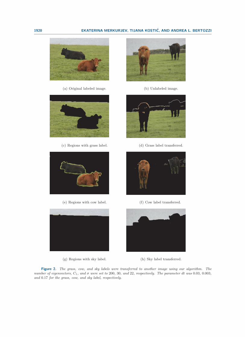
1920 EKATERINA MERKURJEV, TIJANA KOSTIC, AND ANDREA L. BERTOZZI
(a) Original labeled image. (b) Unlabeled image.
(c) Regions with grass label. (d) Grass label transferred.
(e) Regions with cow label. (f) Cow label transferred.
(g) Regions with sky label. (h) Sky label transferred.
Figure 2. The grass, cow, and sky labels were transferred to another image using our algorithm. Thenumber of eigenvectors, C1, and σ were set to 200, 30, and 22, respectively. The parameter dt was 0.03, 0.003,and 0.17 for the grass, cow, and sky label, respectively.

AN MBO SCHEME ON GRAPHS 1921
An affinity matrix is constructed using calculations involving feature vectors. A 16-dimensional feature vector is assigned to each individual, consisting of his/her 16 votes. A“yes” vote is set to 1, a “no” vote is set to −1, while a “did not vote” recording is set to 0.
The weight function used is w(i, j) = e−d(i,j)2
σ2 , where d(i, j) is the 2-norm of the differencebetween the feature vectors of points i and j. The graph is made sparse by setting W (i, j)equal to zero if point j is not among the Mth closest points to point i. The graph is thensymmetrized by setting W (i, j) = max(W (i, j),W (j, i)).
To calculate the eigenvectors, an SVD solver is used. In Step 4 of the algorithm, thefunction u is initialized to 1 for the two Democrats, −1 for the three Republicans, and 0 forthe rest of the Representatives. The three Republicans were chosen to be the first, second,and eighth people in the list. The Democrats were chosen to be the third and fourth peoplein the list. In the fidelity term, λ(x) was set to 1 for each of the five known individuals and 0for the rest.
The parameters C1 (fidelity term parameter), s (in Step 4 of our algorithm), number ofeigenvectors, dt, σ, and M are set to 9.25, 3, 45, 4.675,
√5, and 10, respectively.
We obtained an accuracy of 94.023%. Only 5 iterations in the minimization procedure wereneeded, compared to 450 iterations needed by the method in [8]. Each simulation took about0.7 seconds, and the minimization time was decreased more than 15 times. This informationis shown in Table 1.
Some of the votes predicted the party affiliation very well, i.e., above 85%. We investigatedthe accuracy of our algorithm when these votes were removed. With top two, top six, andtop eight most predictive votes removed, our method obtained an accuracy of 90.1149%,88.34448%, and 81.1494%, respectively. The order of the top eight predictive votes from themost predictive to least predictive is vote 4, 14, 1, 2, 15, 6, 3, and 8.
4. Image inpainting algorithm. The problem of fitting information in the missing pixelsof an image is an important inverse problem in image processing with various applications.Obviously, the goal is to produce a modified image that will look natural to an observer. Theproblem of inpainting may also be seen as the problem of removing occlusive objects from animage. Sparse reconstruction refers to the problem of recovering randomly distributed missingpixels.
There are numerous approaches to solving these problems in the current literature. LocalTV methods became state-of-the-art techniques for image inpainting. However, since they donot perform well on images with high texture, methods that decompose images into cartoonand texture and simultaneously inpaint both have been developed [5, 53]. The problem isalso solved with nonlocal inpainting methods. We are particularly interested in the nonlocalinpainting algorithm from [30] as we develop a computationally efficient nonlocal method.Some very successful nonlocal methods for inpainting and sparse reconstruction are givenin [2] and [24]. Recently, the class of methods that use dictionaries of small patches thatcommonly appear in natural images has become increasingly popular. Those methods, besidesinpainting, are also successful in denoising, as shown in [41]. In addition, a method for imageinpainting using Navier–Stokes fluid dynamics is proposed in [6]. The authors use Navier–Stokes dynamics to propagate isophotes into the inpainting region, thus simulating the waypainting restoration is done. Wavelets and framelets have also been successfully applied to
1922 EKATERINA MERKURJEV, TIJANA KOSTIC, AND ANDREA L. BERTOZZI
solve inpainting problems [16, 11].Our semisupervised image classification algorithm can be modified to inpainting by treat-
ing the inpainted region as unclassified and the rest as the fidelity region. However, sincethere is no information on the inpainted region, we decided to first apply a fast, yet somewhatinaccurate, H1 inpainting algorithm, and then use the result for weight computation. The H1
inpainting method consists of minimizing
(4.1) E(u) =
∫|∇u|2dx+ C
∫λ(x)(u− u0)
2dx,
where λ(x) is 0 on the inpainting region and 1 elsewhere, and u0 is the initial state of theimage. Although the latter algorithm is very fast, it does not perform well on images with hightextures and repetitive structures, nor does it preserve edges [27], something that is achievedby our algorithm.
The algorithm consists of the same four steps:• Create a graph from the data using pixels as vertices, choose a similarity function, and
then create the symmetric graph Laplacian.• Calculate the eigenvectors and eigenvalues of the symmetric graph Laplacian. It is
necessary only to calculate a fraction of the eigenvectors.• Initialize u.• Apply the two-step scheme (to minimize the Ginzburg–Landau functional) detailed in
section 2 for a certain number of iterations until a stopping criterion is satisfied.However, there are some important differences to be discussed in sections 4.1 and 4.2.
Our algorithm is an efficient image inpainting algorithm that is able to correct imageswith repetitive structure or those with high texture content.
4.1. Binary image inpainting. Although the key steps of the classification algorithm re-main the same when it is modified for image inpainting, there are key differences to be noted.
Before the weight matrix is calculated, H1 inpainting is used to preprocess the image. Thematrix W is then built by using a window, or a square-shaped neighborhood around a pixel.We set W (i, j) = 0 for all pixels j that are not in the window of pixel i. Inside the window,W (i, j) = w(i, j), where the weight function is calculated in the same way as in section 3.1.2,i.e., using feature vectors and the Gaussian weight function. No updating of the matrix W isnecessary in the case of binary image inpainting.
The Rayleigh–Chebyshev procedure is used to calculate the eigenvectors and eigenvaluesof the graph Laplacian for binary inpainting. As mentioned before, the Nystrom extensionmethod encounters some problems when dealing with binary images.
In Step 4 of the algorithm, λ(x) in the fidelity term is set to 0 on the inpainting region(which is given the value 0.5 on a 0 to 1 intensity scale) and to 1 on the rest of the image,while u0 is set to 0 on the inpainting region, 1 on the white area, and −1 on the black area.The same stopping criterion is used.
4.2. Grayscale image inpainting. To generalize to gray scale inpainting, we split thesignal bitwise into channels, as in [16],
(4.2) u(x) =7∑
m=0
um(x)2m,
AN MBO SCHEME ON GRAPHS 1923
and inpaint each channel separately. Here um denotes the (m + 1)th component or digit inthe binary representation of the signal, and um ∈ {0, 1} for all x.
A fully connected graph is created in the same way as in section 3.1.2. Again, we firstpreprocess the image using the H1 inpainting algorithm, and use the result to build the matrixW . This weight matrix is used in all eight of the inpainting problems.
The Nystrom extension method is used to calculate the eigenvalues and correspondingeigenvectors since the size of the graph is very large.
In Step 4 of the algorithm, λ(x) in the fidelity term is set to 0 on the inpainting regionand to 1 on the rest of the image. The initialization of u varies with the bit. In the inpaintingregion, u0 is 0, while in the rest of the image, it is 1 on the area where the bit is 1 and −1 onthe area where the bit is 0. The same stopping criterion is used, except α = 0.0001. For someimages, Step 4 is performed for a certain number of iterations.
Updating the matrix W is often necessary for grayscale inpainting, since the adjacencymatrix formed from the preprocessed image using H1 inpainting is usually not good enoughto restore texture and complex patterns, as it contains “bad” regions whose values lie far fromthe true value. In our tests, every few iterations, the matrix is updated using the result fromthe last iteration as the “new image.”
4.3. Inpainting results. We have tested our inpainting algorithm on both binary andgrayscale images. In all cases, we compare our results to the state-of-the-art nonlocal TVinpainting using split Bregman from [62]. Our results are comparable to those achieved usingthe state-of-the-art method, but the timing of the run is significantly reduced (in most casesby about five times).
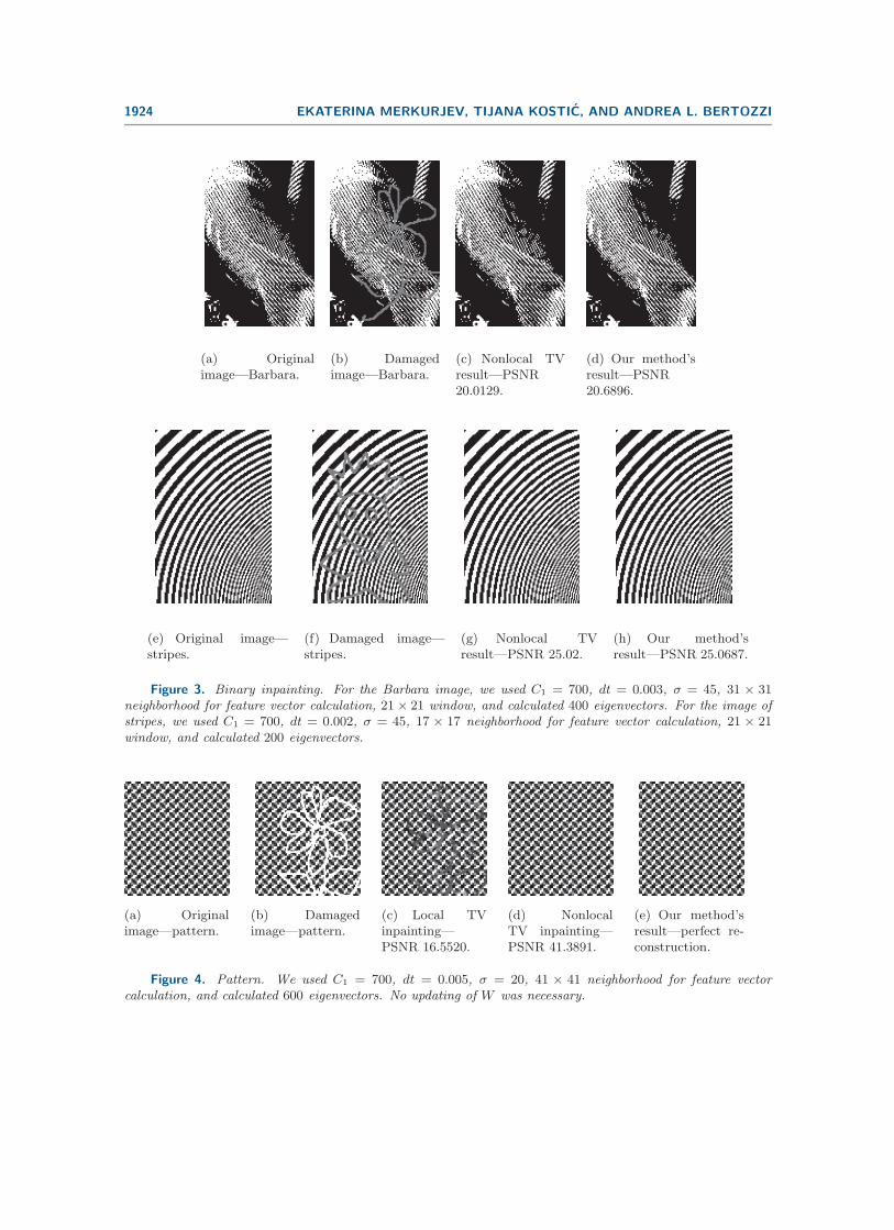
4.3.1. Binary image inpainting results. We applied our algorithm on an image of Barbaraand one of stripes. The results and their PSNR (peak signal-to-noise ratios) are displayed inFigure 3. In both cases, the algorithm was able to recover the texture and repetitive structurepresent in the image, something that is unfeasible for simple algorithms such as local TVinpainting.
4.3.2. Grayscale image inpainting results. We applied our algorithm on an image ofBarbara and a chessboard-like pattern. The goals ranged from removing occlusive objects,such as a flower, text, or a rectangle, to sparse reconstruction. The results along with theirPSNR are displayed in Figures 4–7. Timing and iteration results are displayed in Table 2. Inall cases, repetitive structure and texture were recovered.
We compare our results to local and nonlocal TV inpainting. Local TV inpainting failsto recover texture and repetitive structure. While the results of nonlocal TV inpainting arecomparable to those of our method, our method is more efficient. Timing and iteration resultsare displayed in Table 2. We also show our method and nonlocal TV inpainting at certainiterations in Figure 8. To implement the nonlocal TV inpainting algorithm, we used the splitBregman method detailed in [62] and modified it for inpainting. The stopping condition wasthe same as in our inpainting algorithm, and a quick H1 inpainting algorithm was run on theimage before the weights were calculated.
1924 EKATERINA MERKURJEV, TIJANA KOSTIC, AND ANDREA L. BERTOZZI
(a) Originalimage—Barbara.
(b) Damagedimage—Barbara.
(c) Nonlocal TVresult—PSNR20.0129.
(d) Our method’sresult—PSNR20.6896.
(e) Original image—stripes.
(f) Damaged image—stripes.
(g) Nonlocal TVresult—PSNR 25.02.
(h) Our method’sresult—PSNR 25.0687.
Figure 3. Binary inpainting. For the Barbara image, we used C1 = 700, dt = 0.003, σ = 45, 31 × 31neighborhood for feature vector calculation, 21× 21 window, and calculated 400 eigenvectors. For the image ofstripes, we used C1 = 700, dt = 0.002, σ = 45, 17 × 17 neighborhood for feature vector calculation, 21 × 21window, and calculated 200 eigenvectors.
(a) Originalimage—pattern.
(b) Damagedimage—pattern.
(c) Local TVinpainting—PSNR 16.5520.
(d) NonlocalTV inpainting—PSNR 41.3891.
(e) Our method’sresult—perfect re-construction.
Figure 4. Pattern. We used C1 = 700, dt = 0.005, σ = 20, 41 × 41 neighborhood for feature vectorcalculation, and calculated 600 eigenvectors. No updating of W was necessary.

AN MBO SCHEME ON GRAPHS 1925
(a) Originalimage—Barbara.
(b) Damagedimage—Barbara.
(c) Local TVinpainting—PSNR 32.8517.
(d) NonlocalTV inpainting—PSNR 44.1469.
(e) Our method’sresult—PSNR41.2848.
(f) Originalimage—Barbara.
(g) Damagedimage—Barbara.
(h) Local TVinpainting—PSNR 31.3673.
(i) Nonlocal TVinpainting—PSNR 35.0663.
(j) Our method’sresult—PSNR37.0315.
Figure 5. Rectangle inpainting. For the small rectangle, we used C1 = 700, dt = 0.01, σ = 4, 31 × 31neighborhood for feature vector calculation, and calculated 500 eigenvectors. For the large rectangle, we usedC1 = 700, dt = 0.014, σ = 4, 45×45 neighborhood for feature vector calculation, and calculated 500 eigenvectors.We update W every iteration.
(a) Originalimage—Barbara.
(b) Damagedimage—Barbara.
(c) Local TVinpainting—PSNR 29.1508.
(d) NonlocalTV inpainting—PSNR 35.6896.
(e) Our method’sresult—PSNR34.0688.
Figure 6. Text inpainting. We used C1 = 700, dt = 0.005, σ = 5, 21× 21 neighborhood for feature vectorcalculation, and calculated 500 eigenvectors. We update W every other iteration.

1926 EKATERINA MERKURJEV, TIJANA KOSTIC, AND ANDREA L. BERTOZZI
(a) Originalimage-Barbara.
(b) Damagedimage-Barbara.
(c) Local TVinpainting-PSNR23.6049.
(d) Nonlocal TVinpainting-PSNR27.8196.
(e) Our method’sresult-PSNR27.1651.
(f) Damagedimage-35% of thepixels removed.
(g) Local TVinpainting- PSNR22.6530.
(h) Our method’sresult-PSNR24.1266.
Figure 7. 50% and 35% random inpainting. For the top row, we used C1 = 700, dt = 0.005, σ = 4, 7× 7neighborhood for feature vector calculation, and calculated 400 eigenvectors. We update W every iteration. Forthe bottom row, we used C1 = 700, dt = 0.012, σ = 4, 7 × 7 neighborhood for feature vector calculation, andcalculated 500 eigenvectors. We update W every other iteration.
Table 2Inpainting results comparison.
Total time for Total time for # of iterationsnonlocal TV our method for our method
Binary Barbara 590 s 113 s 6Binary stripes 141 s 66 s 4
Chessboard-like pattern 266 s 48 s 2Text inpainting 410 s 67 s 4Small rectangle inpainting 1882 s 443 s 13Large rectangle inpainting 3397 s 832 s 1350% inpainting 1402 s 333 s 50

AN MBO SCHEME ON GRAPHS 1927
(a) Nonlocal TV,after 2 iter.—PSNR 25.7101.
(b) Nonlocal TV,after 5 iter.—PSNR 30.7031.
(c) Nonlocal TV,after 8 iter.—PSNR 33.2284.
(d) NonlocalTV, after 13iter.—PSNR35.0663.
(e) Our method,after 2 iter.—PSNR 30.4406.
(f) Our method, af-ter 5 iter.—PSNR31.8993.
(g) Our method,after 8 iter.—PSNR 34.4851.
(h) Our method,after 13 iter.—PSNR 37.0315.
Figure 8. Nonlocal TV inpainting and our method at certain iterations.
5. Conclusion. This work presents an algorithm, derived from graph methods and theMBO scheme [43], that links together ideas of graphs and image processing. The results showthat using threshold dynamics in combination with an efficient eigenvalue solver, such as theNystrom extension or the Raleigh–Chebyshev procedure of [1], develops an efficient methodthat can be applied to binary data classification or image processing. In addition, the nonlocalnature of our method allows it to be successful on images with high texture and repetitivestructure.
Garcia-Cardona et al. recently extended this paper’s binary classification algorithm to amulticlass method using the idea of the n-simplex; the model and the results are described in[28]. Hu et al. also built upon the ideas in this paper in [36] by describing a method based onTV for network modularity optimization using the MBO scheme.
Acknowledgments. The authors would like to thank Yanina Landa for providing a MAT-LAB version of the code of the algorithm in [8], and Chris Anderson for providing a code
1928 EKATERINA MERKURJEV, TIJANA KOSTIC, AND ANDREA L. BERTOZZI
for the Raleigh–Chebyshev procedure of [1]. In addition, we thank Arjuna Flenner, Yves vanGennip, Blake Hunter, and Jerome Darbon for useful discussions regarding this work.
REFERENCES
[1] C. Anderson, A Raleigh-Chebyshev procedure for finding the smallest eigenvalues and associated eigen-vectors of large sparse Hermitian matrices, J. Comput. Phys., 229 (2010), pp. 7477–7487.
[2] P. Arias, V. Caselles, and G. Sapiro, A variational framework for nonlocal image inpainting, inProceedings of EMMCVPR 2009, Bonn, Germany, 2009, pp. 345–358.
[3] G. Barles and C. Georgelin, A simple proof of convergence for an approximation scheme for com-puting motions by mean curvature, SIAM J. Numer. Anal., 32 (1995), pp. 484–500.
[4] S. Belongie, C. Fowles, F. Chung, and J. Malik, Partitioning with indefinite kernels using theNystrom extension, in Proceedings of the European Conference on Computer Vision, Copenhagen,2002.
[5] M. Bertalmio, L. Vese, G. Sapiro, and S. Osher, Simultaneous structure and texture inpainting,IEEE Trans. Image Process., 12 (2003), pp. 882–889.
[6] A. Bertozzi, M. Bertalmio, and G. Sapiro, Navier-Stokes fluid dynamics and image and video in-painting, in Proceedings of the IEEE International Conference on Computer Vision and PatternRecognition, 2001, pp. 355–362.
[7] A. Bertozzi, S. Esedoglu, and A. Gillette, Inpainting by the Cahn-Hilliard equation, IEEE Trans.Image Process., 16 (2007), pp. 285–291.
[8] A. Bertozzi and A. Flenner, Diffuse interface models of graphs for classification of high dimensionaldata, Multiscale Model. Simul., 10 (2012), pp. 1090–1118.
[9] A. Buades, B. Coll, and J.-M. Morel, A non-local algorithm for image denoising, in Proceedingsof the IEEE International Conference on Computer Vision and Pattern Recognition, 2005, vol. 2,pp. 60-65.
[10] T. Buhler and M. Hein, Spectral clustering based on the graph p-Laplacian, in Proceedings of the 26thInternational Conference on Machine Learning, 2009, pp. 81–88.
[11] J.-F. Cai, R. Chan, and Z. Shen, A framelet based image inpainting algorithm, Appl. Comput. Harmon.Anal., 24 (2008), pp. 131–149.
[12] T. Chan and L. Vese Active contours without edges, IEEE Trans. Image Process., 10 (2001), pp. 266–277.
[13] F. Chung, Spectral Graph Theory, CBMS Reg. Conf. Ser. Math. 92, Providence, RI, 1997.[14] T. Cour, F. Benezit, and J. Shi, Spectral segmentation with multiscale graph decomposition, in Pro-
ceedings of the IEEE International Conference on Computer Vision and Pattern Recognition, 2005,vol. 2, pp. 1124–1131.
[15] X. Desquesnes, A. Elmoataz, and O. Lezoray, PDEs level sets on weighted graphs, in Proceedingsof the 18th IEEE International Conference on Image Processing (ICIP), 2011, pp. 3377–3380.
[16] J. Dobrosotskaya and A. Bertozzi, A wavelet-Laplace variational technique for image deconvolutionand inpainting, IEEE Trans. Image Process, 17 (2008), pp. 657–663.
[17] P. Drineas and M.W. Mahoney, On the Nystrom method for approximating a Gram matrix for im-proved kernel-based learning, J. Mach. Learn. Res., 6 (2005), pp. 2153–2175.
[18] A. Elmoataz, O. Lezoray, and S. Bougleux, Nonlocal discrete regularization on weighted graphs: Aframework for image and manifold processing, IEEE Trans. Image Process., 17 (2008), pp. 1047–1060.
[19] S. Esedoglu and R. March, Segmentation with depth but without detecting junctions, J. Math. ImagingVision, 18 (2003), pp. 7–15.
[20] S. Esedoglu, S.J. Ruuth, and R. Tsai, Diffusion generated motion using signed distance functions, J.Comput. Phys., 229 (2010), pp. 1017–1042.
[21] S. Esedoglu, S.J. Ruuth, and R. Tsai, Threshold dynamics for high order geometric motions, Inter-faces Free Bound., 10 (2008), pp. 263–282.
[22] S. Esedoglu and Y.R. Tsai, Threshold dynamics for the piecewise constant Mumford-Shah functional,J. Comput. Phys., 26 (2004), pp. 367–384.
[23] L.C. Evans, Convergence of an algorithm for mean curvature motion, Indiana Univ. Math. J., 42 (1993),pp. 553–557.
AN MBO SCHEME ON GRAPHS 1929
[24] G. Facciolo, P. Arias, V. Caselles, and G. Sapiro, Exemplar-based interpolation of sparsely sampledimages, in Proceedings of the Conference on Energy Minimization Methods in Computer Vision andPattern Recognition, Bonn, Germany, 2009, pp. 331–344.
[25] C. Fowlkes, S. Belongie, and J. Malik, Spectral grouping using the Nystrom method, IEEE Trans.Pattern Anal. Mach. Intell., 28 (2006), pp. 469–475.
[26] C. Fowlkes, S. Belongie, F. Chung, and J. Malik, Efficient spatiotemporal grouping using theNystrom method, in Proceedings of the IEEE Computer Society Conference on Computer Vision andPattern Recognition, HI, 2001, pp. 214–225.
[27] C. Frohn-Schauf, S. Henn, and K. Witsch, Nonlinear multigrid methods for total variation imagedenoising, Comput. Vis. Sci., 7 (2004), pp. 199–206.
[28] C. Garcia-Cardona, E. Merkurjev, A.L. Bertozzi, A. Flenner, and A. Percus, Fast multiclasssegmentation using diffuse interface methods on graphs, IEEE Trans. Pattern Anal. Mach. Intell.,submitted.
[29] G. Gilboa and S. Osher, Nonlocal operators with applications to image processing, Multiscale Model.Simul., 7 (2008), pp. 1005–1028.
[30] G. Gilboa and S. Osher, Nonlocal linear image regularization and supervised segmentation, MultiscaleModel. Simul., 6 (2007), pp. 595–630.
[31] T. Goldstein and S. Osher, The split Bregman method for L1-regularized problems, SIAM J. ImagingSci., 2 (2009), pp. 323–343.
[32] T. Goldstein, X. Bresson, and S. Osher, Geometric applications of the split Bregman method: Seg-mentation and surface reconstruction, J. Sci. Comput., 45 (2010), pp. 272–293.
[33] L. Grady and E.L. Schwartz, Isoperimetric graph partitioning for image segmentation, IEEE Trans.Pattern Anal. Mach. Intell., 28 (2006), pp. 469–475.
[34] A. Harten, High resolution schemes for hyperbolic conservation laws, J. Comput. Phys., 49 (1983),pp. 357–393.
[35] H. Hein and T. Buehler, An inverse power method for nonlinear eigenproblems with applications in1-spectral clustering and sparse PCA, Adv. Neural Inform. Process. Syst., 23 (2010), pp. 847–855.
[36] H. Hu, T. Laurent, M.A. Porter, and A.L. Bertozzi, A method based on total variation for networkmodularity optimization using the MBO scheme, SIAM J. Appl. Math., (2013), submitted.
[37] D. Karger, and C. Stein, A new approach to the minimum cut problem, J. ACM, 43 (1996), pp. 601–640.
[38] D. Karger, Minimum cuts in near-linear time, J. ACM, 47 (2000), pp. 46–76.[39] R.V. Kohn and P. Sternberg, Local minimizers and singular perturbations, Proc. Roy. Soc. Edinburgh
Sect. A, 11 (1989), pp. 69–84.[40] Y. Lou, X. Zhang, S. Osher, and A. Bertozzi, Image recovery via nonlocal operators, J. Sci. Comput.,
42 (2010), pp. 185–197.[41] J. Mairal, M. Elad, and G. Sapiro, Sparse representation for color image restoration, IEEE Trans.
Image Process., 17 (2008), pp. 53–69.[42] B. Merriman and S.J. Ruuth, Diffusion generated motion of curves on surfaces, J. Comput. Phys.,
225 (2007), pp. 2267–2282.[43] B. Merriman, J. Bence, and S. Osher, Diffusion generated motion by mean curvature, in Proceedings
of the Computational Crystal Growers Workshop, Providence, RI, 1992, pp. 73–83.[44] E. Mezuman and Y. Weiss, Globally optimizing graph partitioning problems using message passing, in
Proceedings of the 15th International Conference on Artificial Intelligence and Statistics, 22, 2012,pp. 770–778.
[45] B. Mohar, The Laplacian spectrum of graphs, Graph Theory Combin. Appl., 2 (1991), pp. 871–898.[46] D. Mumford and J. Shah Optimal approximations by piecewise smooth functions and associated vari-
ational problems, Comm. Pure Appl. Math., 42 (1989), pp. 577–685.[47] M.M. Naeini, G. Dutton, K. Rothley, and G. Mori, Action recognition of insects using spectral
clustering, in Proceedings of the IAPR Conference on Machine Vision Applications, 2007, pp. 1–4.[48] S.Osher and J. Shen, Digitalized PDE method for data restoration, in Analytical-Computational Meth-
ods in Applied Mathematics, E.G.A. Anastassiou, ed., Chapman & Hall/CRC, New York, 2000,pp. 751–771.
[49] G. Peyre, S. Bougleux, and L. Cohen, Non-local regularization of inverse problems, in Proceedingsof the European Conference on Computer Vision (ECCV 2008), Springer, Berlin, 2008, pp. 57–68.
1930 EKATERINA MERKURJEV, TIJANA KOSTIC, AND ANDREA L. BERTOZZI
[50] C.A. Ratanamahatana and D. Gunopulos, Scaling up the naive Bayesian classifier: Using decisiontrees for feature selection, in Proceedings of the IEEE International Conference on Data Mining(ICDM 2002), Maebashi, Japan, 2002, pp. 475–487.
[51] J. Rubinstein, P. Sternberg, and J.B. Keller, Fast reaction, slow diffusion, and curve shortening,SIAM J. Appl. Math., 49 (1989), pp. 116–133.
[52] S.J. Ruuth, Efficient algorithms for diffusion-generated motion by mean curvature, J. Comput. Phys.,144 (1998), pp. 603–625.
[53] H. Schaeffer and S. Osher, A low patch-rank interpretation of texture, SIAM J. Imaging Sci., 6 (2013),pp. 226–262.
[54] J. Shi and J. Malik, Normalized cuts and image segmentation, IEEE Trans. Pattern Anal. Mach. Intell.,22 (2000), pp. 888–905.
[55] M. Stoer and F. Wagner, A simple min-cut algorithm, J. ACM, 44 (1997), pp. 585–591.[56] A. Szlam and X. Bresson, Total variation-based graph clustering algorithm for Cheeger ratio cuts, in
Proceedings of the 27th International Conference on Machine Learning, 2010, pp. 1039–1046.[57] Y. van Gennip and A.L. Bertozzi, Γ-convergence of graph Ginzburg–Landau functionals, Adv. Differ-
ential Equations, 17 (2012), pp. 1115–1180.[58] Y. van Gennip, N. Guillen, B. Osting, and A.L. Bertozzi, Mean curvature, threshold dynamics,
and phase field theory on finite graphs, (2013) (journal unknown).[59] U. von Luxburg, A tutorial on spectral clustering, Statist. Comput., 17 (2007), pp. 395–416.[60] D. Wagner and F. Wagner, Between min cut and graph bisection, in Mathematical Foundations of
Computer Science 1993, Lecture Notes in Comput. Sci. 711, Springer, New York, 1993, pp. 744–750.[61] L. Zelnik-Manor and P. Perona, Self-tuning spectral clustering, Adv. Neutral Inform. Process. Syst.,
17 (2004), pp. 1601–1608.[62] X. Zhang, M. Burger, X. Bresson, and S. Osher, Bregmanized nonlocal regularization for deconvo-
lution and sparse reconstruction, SIAM J. Imaging Sci., 3 (2010), pp. 253–276.[63] X. Zhang and T. Chan, Wavelet inpainting by nonlocal total variation, Inverse Problems Imag., 4
(2010), pp. 1–20.[64] D. Zhou and B. Scholkopf, Regularization on discrete spaces, in Pattern Recognition, Springer, Berlin,
Germany, 2005, pp. 361–368.[65] D. Zhou and B. Scholkopf, Discrete regularization, in Semi-Supervised Learning, MIT Press, Cam-
bridge, MA, 2006, pp. 221–232.[66] D. Zhou, J. Huang, and B. Scholkopf, Learning from labeled and unlabeled data on a directed graph,
in Proceedings of the 22nd International Conference on Machine Learning, 2005, pp. 1041–1048.[67] D. Zhou, B. Scholkopf, and T. Hofmann, Semi-supervised learning on directed graphs, Adv. Neutral
Inform. Process. Syst., 17 (2005), pp. 1633–1640.