an old lecture about gw approximation

. .

Electronic Excitations and Spectroscopy:Theory and Codes

Introductionto the

GW approximation

Fabien Bruneval

Service de Recherche de Metallurgie Physique, CEA Saclay, France

December 12, 2007

GW approximation Fabien Bruneval

. .

Outline

1 Band structure & calculations

2 Theory: from Hartree-Fock to GWFunctional approach to the MB problemHedin’s equations

3 Physical content of GWWhat does the screening account for?What does the self-energy contain?

4 GW for realistic materialsImplementationApplications


. .Band structure & calculations

Outline







Band structure from one particle approximations

Any one-particle Hamiltonian: h(r)→ diagonalizationh(r)φi (r) = εiφi (r)and εi is called the band structure.

HOWEVER, in reality,

H(r1, ..., rN) =∑

i

−∇i

2

2

+∑

i

Vnuclei(ri ) +∑i<j

1

|ri − rj |

→ ionization or affinity energy



Photoemission spectroscopy

hν

E kin Energy conservation:

Before the experimenthν + EN,0

After the experimentEkin + EN−1,i

hν − Ekin = EN−1,i − EN,0=− εi→ ionization energy or binding energy or valence band structure



Wavefunctions methods

Hartree-Fock method: variationally best Slater determinant

ΦN,0(r1, ..., rN) ∝

∣∣∣∣∣∣∣∣∣φ1(r1) . . . φN(r1)φ1(r2) . . . φN(r2)

......

φ1(rN) . . . φN(rN)

∣∣∣∣∣∣∣∣∣made of N one-particle wavefunctions φi .

L = 〈Φ|H|Φ〉 −∑

i

εHFi

∫dr|φi (r)|2

⇒ hHFφi = εHFi φi

εHFi obtained as N Lagrange multipliers



Hartree-Fock method

Valence Photoemission:

ΦN−1,i (r1, ..., rN−1) ∝∣∣∣∣∣∣∣∣∣φ1(r1) . . . φi−1(r1) φi+1(r1) . . . φN(r1)φ1(r2) . . . φi−1(r2) φi+1(r2) . . . φN(r2)

......

φ1(rN−1) . . . φi−1(rN−1) φi+1(rN−1) . . . φN(rN−1)

∣∣∣∣∣∣∣∣∣Koopmans theorem:

εi = 〈N, 0|H|N, 0〉 − 〈N − 1, i |H|N − 1, i〉

The eigenvalues εi do have a physical meaningApproximation: No relaxation of the other orbitals



Hartree-Fock results

Atoms

Ionization energy

0 5 10 15 20 25experimental ionization energy (eV)

0

5

10

15

20

25

calc

ulat

ed io

niza

tion

ener

gy (e

V)

Li

Ne

B

F

N

Be

O

He

H

C

calculated as the energy of the HOMO with gaussian 03




Homogeneous electron gas (=jellium) with constant density ρ0

2 3 4 5 6rs

0

2

4

6

8

10

12

14

16

Occ

upie

d ba

nd w

idth

(eV

)

Free electronHartree-Fock

0 0.5 1 1.5 2k / kF

E ( k

)

Aluminu

m

Sodium

EF

W




Band gap of semiconductors and insulators

courtesy of Brice Arnaud, Universite de Rennes, FranceGW approximation Fabien Bruneval


Density Functional Theory

DFT well assessed for the structure of solids

BUT

L = 〈Φ|HKS|Φ〉 −∑

i

εKSi

∫dr|φKS

i (r)|2

⇒ hKS(r)φKSi (r) = εKS

i φKSi (r)

εKSi obtained as N Lagrange multipliers

Kohn-Sham energies cannot be interpreted as removal/additionenergies



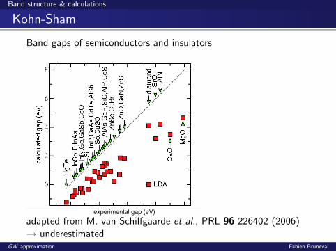
Kohn-Sham

Band gaps of semiconductors and insulators

experimental gap (eV)

adapted from M. van Schilfgaarde et al., PRL 96 226402 (2006)→ underestimated



The solution?

Need for a tool that gives the correct band structure εii.e. the correct differences EN,0 − EN±1,i

⇒ Green’s functions


. .Theory: from Hartree-Fock to GW

Outline







Green’s functions: from HF to GW

Review the many-body equations with a functional approach(Hedin 1965)

Convince you that GW is a natural extension beyond HF

use of zero temperature Green’s function formalism:

iG (1, 2) = 〈N, 0|T[ΨH(1)Ψ†

H(2)]|N, 0〉

=

{〈N, 0|ΨH(1)Ψ†

H(2)|N, 0〉 if t1 > t2−〈N, 0|Ψ†

H(2)ΨH(1)|N, 0〉 if t1 < t2.



Green’s functions: from HF to GW

t1 > t2

〈N, 0|ΨH(1)Ψ†H(2)|N, 0〉

Ψ†H(2)|N, 0〉

Ψ†H(1)|N, 0〉

( r , t )

( r , t )

2 2

1 1

t1 < t2

〈N, 0|Ψ†H(2)ΨH(1)|N, 0〉

ΨH(2)|N, 0〉ΨH(1)|N, 0〉

( r , t )

( r , t )

2 2

1 1



Functional approach to the MB problem

To determine the 1-particle Green’s function

[i∂

∂t− h0]G + i

∫vG2 = 1

where h0 = −12∇

2 + vext is the independent particle Hamiltonian.

The 2-particle Green’s function describes the motion of 2 particles.Unfortunately, a whole hierarchy of equations:

G1(1, 2) ← G2(1, 2; 3, 4)G2(1, 2; 3, 4) ← G3(1, 2, 3; 4, 5, 6)

......

...



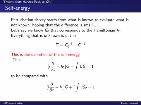
Self-energy

Perturbation theory starts from what is known to evaluate what isnot known, hoping that the difference is small...Let’s say we know G0 that corresponds to the Hamiltonian h0

Everything that is unknown is put in

Σ = G−10 − G−1

This is the definition of the self-energyThus,

[i∂

∂t− h0]G −

∫ΣG = 1

to be compared with

[i∂

∂t− h0]G + i

∫vG2 = 1



Functional derivation of the MB problem

Trick due to Schwinger (1951):introduce a small external potential U(3), that will be made equalto zero at the end, and calculate the variations of G1 with respectto USelf-energy

Σ(1, 2) = −i

∫d3d4v(1+, 3)G (1, 4)

δG−1(4, 2)

δU(3)

Vertex function

Γ(1, 2; 3) = −δG−1(1, 2)

δU(3)

Dyson equation

G−1(1, 2) = G−10 (1, 2)− U(1)δ(1, 2)− Σ(1, 2)



Functional definition of the self-energy

Exact equations

G−1 = G−10 − Σ

Σ = iGvΓ

Γ = 1 +

[−iv +

δΣ

δG

]GGΓ

Γ(0) = 1

Σ(1) = iGv = Σx

→ Hartree Fock approximation

G

v



Functional definition of the self-energy

Exact equations

G−1 = G−10 − Σ

Σ = iGvΓ

Γ = 1 +

[−iv +

δΣ

δG

]GGΓ

Σ(1) = iGv

Γ(1) = 1 + ivGGv + ivGvG

Σ(2) = Σx − GvGGv − GvGvG

→ 2nd order in vGW approximation Fabien Bruneval


GW origins



Need for screening

A[U] = G [U] or Γ[U] or Σ[U]

variations of some operator with respect to a local bareperturbation: δA

δU

δU(r) = e (r−r )δ 0



Need for screening

Purely classical interaction

δU(r) = e (r−r )δ

V(r) = U(r) + classical screeningδ δ

0

δV (1) = δU(1) +

∫d2v(1, 2)δρ(2)

the variations of the charge density δρ tends to oppose to theperturbation.



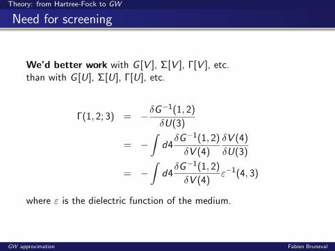
Need for screening

We’d better work with G [V ], Σ[V ], Γ[V ], etc.than with G [U], Σ[U], Γ[U], etc.

Γ(1, 2; 3) = −δG−1(1, 2)

δU(3)

= −∫

d4δG−1(1, 2)

δV (4)

δV (4)

δU(3)

= −∫

d4δG−1(1, 2)

δV (4)ε−1(4, 3)

where ε is the dielectric function of the medium.



Towards Hedin’s equations

Σ = iGvε−1Γ

irreducible vertex

Γ = −δG−1

δV

= 1 +δΣ

δGGG Γ

screened Coulomb interaction

W = ε−1v

dielectric functionε = 1− v χ

irreducible polarizability

χ =δρ

δV= −iGG Γ



Hedin’s equations

Σ = iGW Γ

Γ = 1 +δΣ

δGGG Γ

W = ε−1v

ε = 1− v χ

χ = −iGG Γ

G−1 = G−10 − Σ

Hedin’s wheel

Σ

Γ

W G

χ~ ~

Σ(0) = 0

Γ(1) = 1

χ(1) = −iGG = χRPA

Σ(1) = iGW

G

W



GW for the jellium

Homogeneous electron gas with constant density ρ0

2 3 4 5 6rs

0

2

4

6

8

10

12

14

16

Occ

upie

d ba

nd w

idth

(eV

)

Free electronHartree-FockGW

0 0.5 1 1.5 2k / kF

E ( k

)

Aluminu

m

Sodium

EF

W


. .Physical content of GW

Outline







From the Coulomb interaction to the screened Coulombinteraction

Hartree-Fock self-energy

Σ(1, 2) = iG (1, 2)v(1+, 2)

GW self-energy

Σ(1, 2) = iG (1, 2)W (1+, 2)

The only difference is in the v or W



What is different in v and in W

W is shorter ranged than vwith a crude model for W in metal:

W (r1, r2) =e−λTF .|r1−r2|

|r1 − r2|

v is static, whereas W is dynamic

v(r1, r2, t1 − t2) = δ(t1 − t2)1

|r1 − r2|

W (r1, r2, t1 − t2)



How does W look like?

W in frequency domain can be calculated and alsomeasured!

Silicon

It can be measured by EELS, IXSS.GW approximation Fabien Bruneval


How does W look like?

In real time:Macroscopic response to U(1) = eδ(r1)δ(t1)

-10 0 10τ (a.u.)

Re {

W -

v}



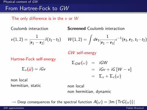
From Hartree-Fock to GW

The only difference is in the v or W

Coulomb interaction

v(1, 2) =1

|r1 − r2|δ(t1−t2)

Screened Coulomb interaction

W (1, 2) =

∫dr3

1

|r1 − r3|ε−1(r3, r2, t1−t2)

Hartree-Fock self-energy

Σx(ω//) = iGv

non localhermitian, static

GW self-energy

ΣGW (ω) = iGW

= iGv + iG [W − v ]

= Σx + Σc(ω)

non localnon hermitian, dynamic

→ Deep consequences for the spectral function A(ω) = |Im {TrG (ω)}|GW approximation Fabien Bruneval


Spectral function

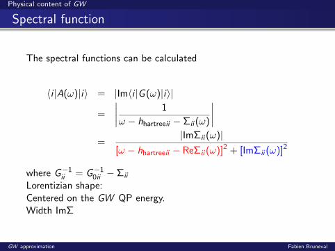
The spectral functions can be calculated

〈i |A(ω)|i〉 = |Im〈i |G (ω)|i〉|

=

∣∣∣∣ 1

ω − hhartreeii − Σii (ω)

∣∣∣∣=

|ImΣii (ω)|[ω − hhartreeii − ReΣii (ω)]2 + [ImΣii (ω)]2

where G−1ii = G−1

0ii − Σii

Lorentizian shape:Centered on the GW QP energy.Width ImΣ



From Hartree-Fock to GW

A(ω) = |ImG (ω)|

ω

Aii

Non-interacting electronsInteracting electrons

Re Σii

Im Σii

Satellite

Zi



Solution of the quasiparticle equation

Silicon

-20

-16

-12

-8

-4

0

Re Σ

(eV

)

Re Σ ( ωii )ω − hii

-40 -20 0 20 40ω (eV)

0

0.02

0.04

0.06

0.08

0.1

| Im

G |

Aluminum

-60

-50

-40

-30

-20

-10

0

Re Σ

(eV

)

Re Σii ( ω )ω - hii

-40 -20 0 20 40ω (eV)

0

0.1

0.2

0.3

0.4

0.5

0.6

0.7

0.8

| Im

G |



Lifetime and GW self-energy

Hole self-energy:

Im{〈i |Σ(εi )|i〉} = −∑

jqGG′

Mij(q + G)M∗ij (q + G′)

× Im(W − v)GG′(q, εj − εi )

× θ(µ− εj)θ(εj − εi )

µ

εi


. .GW for realistic materials

Outline







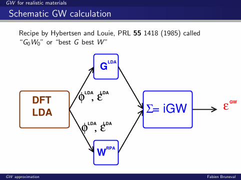
Schematic GW calculation

Recipe by Hybertsen and Louie, PRL 55 1418 (1985) called“G0W0” or “best G best W ”

φ , εLDA LDA

DFTLDA

φ , εLDA LDA

GLDA

W

Σ= iGW

RPA

εGW



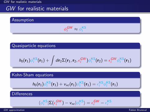
GW for realistic materials

Assumption

φGWi ≈ φKS

i

Quasiparticle equations

h0(r1)φGWi (r1) +

∫dr2Σ(r1, r2, ε

GWi )φGW

i (r2) = εGWi φGW

i (r1)

Kohn-Sham equations

h0(r1)φKSi (r1) + vxc(r1)φ

KSi (r1) = εKS

i φKSi (r1)

Differences

〈φKSi |Σ(εGW

i )− vxc |φKSi 〉 = εGW

i − εKSi



GW for realistic materials

Assumption

φGWi ≈ φKS

i

Quasiparticle equations

h0(r1)φKSi (r1) +

∫dr2Σ(r1, r2, ε

GWi )φKS

i (r2) = εGWi φKS

i (r1)

Kohn-Sham equations

h0(r1)φKSi (r1) + vxc(r1)φ

KSi (r1) = εKS

i φKSi (r1)

Differences

〈φKSi |Σ(εGW

i )− vxc |φKSi 〉 = εGW

i − εKSi



G0W0 calculation

To calculate the GW self-energy:

Σ(1, 2) = iG (1, 2)W (1+, 2)

which is Fourier transformed into frequencies

Σ(r1, r2, ω) = i

∫dω′G (r1, r2, ω + ω′)W (r1, r2, ω

′)

We need the following ingredients:

The KS Green’s function: G (r1, r2, ω) =∑

iφKS

i (r1)φKS∗i (r2)

ω−εKSi ±iη

The RPA dielectric matrix: εRPA −1GG′ (q, ω)



Band gaps of semiconductors

experimental gap (eV)

from M. van Schilfgaarde et al., PRL 96 226402 (2006).GW approximation Fabien Bruneval


Result for a complex metal

Nickel

from F. Aryasetiawan, PRB 46 13051 (1992).GW approximation Fabien Bruneval


Surfaces

Al(111): potential

from I.D. White et al, PRL 80, 4265 (1998).



References

L. Hedin, Phys. Rev. 139 A796 (1965).

L. Hedin and S. Lunqdvist, in Solid State Physics, Vol. 23(Academic, New York, 1969), p. 1.

F. Aryasetiawan and O. Gunnarsson, Rep. Prog. Phys. 61237 (1998).

W.G. Aulbur, L. Jonsson, and J.W. Wilkins, Sol. State Phys.54 1 (2000).

G. Strinati, Riv. Nuovo Cimento 11 1 (1988).

www.abinit.org

theory.polytechnique.fr/people/bruneval/


an old lecture about gw approximation

Documents