an open-source its platform - aalborg universitetdbtr.cs.aau.dk/dbpublications/dbtr-32.pdf · an...

An Open-Source ITS Platform

Ove Andersen and Kristian Torp

August 2012

TR-32

A DB Technical Report

Title An Open-Source ITS Platform Copyright © 2012 Ove Andersen and Kristian Torp. All rights reserved

Author(s)


Publication History

August 2012. A DB Technical Report

For additional information, see the DB TECH REPORTS homepage: <www.cs.auc.dk/DBTR>

Any software made available via DB TECH REPORTS is provided “as is” and without any express or

implied warranties, including, without limitation, the implied warranty of merchantability and

fitness for a particular purpose.

The DB TECH REPORTS icon is made from two letters in an early version of the Rune alphabet,

which was used by the Vikings, among others. Runes have angular shapes and lack horizontal lines

because the primary storage medium was wood, although they may also be found on jewelry, tools,

and weapons. Runes were perceived as having magic, hidden powers. The first letter in the logo is

“Dagaz,” the rune for day or daylight and the phonetic equivalent of “d.” Its meanings include

happiness, activity, and satisfaction. The second letter is “Berkano,” which is associated with the

birch tree. Its divinatory meanings include health, new beginnings, growth, plenty, and clearance. It

is associated with Idun, goddess of Spring, and with fertility. It is the phonetic equivalent of “b.”

1

An Open-Source ITS Platform


Department of Computer Science

Aalborg University

Selma Lagerlöfs Vej 300, 9220 Aalborg Øst, Denmark

{xcalibur, torp}@cs.aau.dk

Abstract

In this report a complete system used to compute travel-times from GPS data is described. Two approaches

to computing travel time are proposed one based on points and one based on trips. Overall both

approaches gives reasonable results compared to existing manual estimated travel times. However, the

trip-based approach requires more GPS data and of a higher quality than the point-based approach. The

system has been completely implemented using open-source software and is in production. A detailed

performance study, using a desktop PC, shows that the system can handle large data sizes and that the

performance scales, for some components, linearly with the number of processor cores available. The main

conclusion is that large quantity of GPS data can, with a very limited budget, used for estimating travel

times, if enough GPS data is available.

2

1 Introduction There is a great public interest in know the estimated travel-time between two points as examples global

companies such as Google and Microsoft provides this information freely with their online map services.

However, the current services have a general shortage because they are bad at taking rush-hours into

consideration, further they have generally insufficient coverage of the smaller roads. Combined these

shortages results in that the estimated travel-times are to inaccurate to be useful for detailed scheduling of

vehicles.

In this report an open-source based Intelligent Transport System (ITS) platform for accurately estimating

travel-time is introduced in great details. The ITS platform uses GPS data as the foundation for estimating

travel-time. The report uses a major Danish transport organization called FlexDanmark as a case study.

However, none of the solutions presented in the report are specific to FlexDanmark or Denmark.

FlexDanmark is a company that organizes demand-driven transport. FlexDanmark uses several parameters

in their optimization of the transports, such as the best experience for the passengers at the lowest

expense and waste of time for the drivers. The organization is mainly done by estimating how long time a

transport takes. The more precise FlexDanmark can estimate a transport, the better they can plan. To

calculate the duration of a transport, FlexDanmark makes use of two types of data:

A map of all road segments in Denmark. Every road segment is associated with values estimating

the average speed driven on the road segment during different periods of time, e.g., during peak

and non-peak traffic times. From this map, it is possible to calculate how long time a predefined

route will take using the speeds associated with each road segment. This data set is called a speed

map.

A matrix, containing information on the distance and travel time between 13.578 regions, or points

of interests (POIs). This data set is called a drive-time matrix.

Both set of data are used because of a trade-off between computation time and accuracy; the speed map is

slow to use but more accurate and the drive-time matrix is fast to use but less accurate.

Using these two data sets FlexDanmark can estimate the travel time of all trips. The disadvantages of two

data sets are that they are static and manually defined. This means that the average speeds on the road

segments are defined in groups of road categories, thus the actual average speed on a segment can be

significantly different from the manually estimated speed.

To improve the accuracy of the estimates of travel times, FlexDanmark needs tools that can make custom

reports on for example different periods of a day or on specific weekdays. The improved estimates must be

based on real-world data instead of manually defined data.

A good way to estimate the travel time of a trip is to base the estimate on measurement from previous

similar trips. FlexDanmark already manages GPS data logs reporting the time, position, and speed of the

vehicles used. This GPS data is stored in a database and is an excellent source for estimating travel times (1)

(2). With GPS data it is possible to make estimates depending on day and time, e.g., comparing rush hour to

non-rush hour. In addition, when basing estimates on real-world data the estimates are objective and it is

3

unnecessary to argue about the quality of these estimates. This is a problem with the current estimates

that can be considered subjective since they are based mostly on experience.

In this report, a complete architecture is presented for transforming the GPS data into a data warehouse

that can be used to estimate travel times. The complete architecture consists of a data warehouse, custom

ETL software, and an interface to third-party software. The architecture is fully implemented in an open-

source software stack. The system has been used in production since 1st of March 2011.

The report is organized as follows. First, related work is discussed and then a larger running example is

introduced. Then a complete data-warehouse design is presented in details. The next topic is a description

of the software architecture, in particular the open-source components used. Next, the details of the

implementation are presented. This includes inter-process communication, ETL, and the various outputs

produced by the platform. The complete system is implemented and a section is dedicated to performance

experiments. This is followed by the conclusion.

1.1 Objective and Contributions The objective of this system is to provide a system that can provide:

A speed map for a complete road network.

A matrix of shortest travel times between all points of interest (POIs).

The contributions of the report are the following.

Figure 1: Data Flow of the Complete System

A complete system that uses GPS data for generating a speed map of Denmark along with travel

times and length of about 184 million different routes between the POIs in Denmark.

A generic system in the sense that it takes a map, GPS data, and POIs as input and returns speed

maps and travel times as output, as shown by Figure 1. Anyone with similar input data can get

output for the parts of the world covered by the input data.

A cost-efficient system is provided because the complete system can be executed on a modern

desktop computer. Some parts of the system is though optimized for parallel computing, thus the

more processors (and memory) available, the better performance will be archived. However the

system is effective on standard, low-price hardware.

4

A complete open-source system that is capable of running on a wide range of operating systems

(64 bit required though, for utilizing more than 2GB of memory pr. application), only limited by the

requirements of being able to compile C++ code and running Python code with its dependencies.

A complete data warehouse implementation for storing GPS data. This solution is used daily by

2,000-3,000 taxi drivers (almost 10,000 unique vehicles IDs).

A system for the entire road network of Denmark has been used as map. Thus this system has

provided the first complete speed map of Denmark based on real-world GPS data.

2 Related Work The related work can be divided into two main parts; a tool-oriented part and a theoretical/academic part.

The two parts of related work are described in separate sections.

2.1 Tools KTH Royal Institute of Technology and IBM have implemented a system in Stockholm that utilizes real-time

traffic information to better manage transportation (3) (4). The data have been collected primarily from

GPS devices installed in taxis. The system is said to reduce traffic by 20 percent in the city and reduce travel

time by almost 50 percent. The system is not open source and details about the implementation is not

available

Google is also interested in the growing sizes of GPS data becoming available. Today Google is a large player

in the market of maps, navigation, and traffic management. Google gets traffic data from several places,

but the most interesting data source is all the mobile users with GPS devices that can transmit their

location data to Google (5). Google collects this data in real-time and uses these for several purposes. First

of all, Google Maps Navigation can plan a route that automatically leads a driver away from current traffic

congestions (6). Also Google Maps can predict traffic conditions on major roads based on the congestion

history (7). The service is though not available for all countries yet and the access to the data is restricted.

Google has though withdrawn their GPS solution from route prediction (8), apparently due to the feature

not working as expected, though it is said that the service still work on handheld devices.

TomTom has a similar service to Google, named TomTom HD Traffic (9). This service collects GPS data from

TomTom devices and uses this information along with other traffic-related information to guide drivers

away from congested areas. TomTom also provides an online real-time speed map with route planning

features that takes historical data into account (10). It seems like the TomTom service is currently only very

limited used as only very little live data is available.

2.2 Academic Generating a map from GPS data has been done by (11). The map is dynamic in the context of time,

meaning that the values such travel-time varies over time. The outset is a large set of historical data

generated from vehicles. From the GPS data a graph is generated that describes the road network at

different periods having the weights of road segments representing the speeds of the road segment at a

certain time. These historical data is used to analyze the trends of the road map over time and to find

trends in the travel-time. When data does not cover the entire road network methods for estimating the

travel-time are presented, which results in a complete coverage.

5

The measurement of congestion is the main topic of (12). The paper uses GPS data to compute vehicle

speeds and travel times. From this information the congestion levels on urban road networks are

estimated. The paper also examines how such GPS data can be integrated into an ITS platform for making

easy and intelligent road network congestion monitoring.

The need for intelligent transport planning arises, when more real-time traffic information becomes

available, according to (13). The paper presents a dynamic planning framework that can communicate with

the drivers when new transportations are being planned. In addition, routes of ongoing trips can be

recalculated if the traffic situation changes. The paper does not utilize GPS data but other traffic

notifications received by traffic management centers.

Real-time data has been used to discover traffic incidents by (14). This paper utilizes GPS data from taxis to

recognize the traffic situation in the city of Berlin, Vienna, and Nuremberg. The GPS data is logged at least

once per minute and is sent back to a central site. Here the data is analyzed and used to determine the

current flow in the traffic. Using GPS data from a large set of taxis, the entire main road network of the

cities are covered. This real-time system is in production.

Other sources for computing speed maps and travel times exist such as induction loops. The paper (15) is a

case study of the San Francisco area. Here data from induction loops is compared to GPS data from probe

vehicles. The paper concludes that travel times can be computed within an error of 10% using GPS probe

data, induction loops, or a mixture of both, when comparing to number plate recognition travel times.

3 Running Example The section describes various types of GPS data in particular how to combine GPS data into trips are

considered. Map-matching of GPS data to a digital map is described and the basic idea for estimating

travel-time from GPS data is presented.

3.1 External Influence on Travel Time A road network is a very dynamic environment where the speed of a vehicle is dependent on a number of

factors, e.g., the congestion level, the vehicle type, the weather, and road-construction work. The external

influences that are taken into consideration in the project are described in this section.

The travel time on the road segments vary depending on hours, weekdays, and seasons. Rush-hours are a

major concern because they reoccur every workday and the travel time during rush hours can be much

longer than outside rush hours. Saturdays and Sundays are not regular working days, thus they cannot be

treated like workdays and this needs to be taken into account. Date and time information is provided in the

GPS data used therefore rush hours are taken into consideration.

The type of vehicle, e.g., a bus, truck, taxi, has an impact on the travel time of two reasons. Firstly, the

different vehicle types have different acceleration profiles, top speeds, and maneuverability’s. Secondly,

speed limits are different for different vehicles types. As an example, the speed limit for busses is lower

than for taxis on freeways. For all data a unique vehicle ID is provided. However, only a small subset of the

GPS data available contains information on the vehicle type. The unique vehicle IDs are stored such that the

6

data can later be augmented with the vehicle type information if such information should become

available.

The GPS data is recorded using off-the-shelf devices. This means that the positions recorded are not

accurate and if these positions are used without any corrections it may lead to imprecisions. To improve

the accuracy of the GPS data a map is used to correct GPS position such that (most) positions are on a road.

This correction of the GPS positions is called map matching.

Other external influences on travel time are weather conditions and road network situations. If a region is

covered in snow for a period, the travel times will definitely be different than warmer periods. The same

applies if a main road is closed for repair. Such conditions are not taken into account, since they are

unpredictable, momentary and the impact on the traffic situation will be different for each event. In

addition, such data are not available to this project.

3.2 Points versus Trip The GPS data contains a vehicle id, latitude, longitude, timestamp, speed, direction, and other less relevant

information. Because a vehicle id is available the GPS data can be handled in two ways as single points or

grouped into trips. The point and the trip approach are explained in details in the following.

3.2.1 Points

When GPS data is order by vehicle id and timestamp, it is possible to calculate an average speed for each

segment in a map with only a single scan of the GPS data. First of all, each GPS point has to be map-

matched to a segment, and then the average speed for each segment can then be calculated.

Figure 2: Example of GPS Points Map-matched to a Road Network.

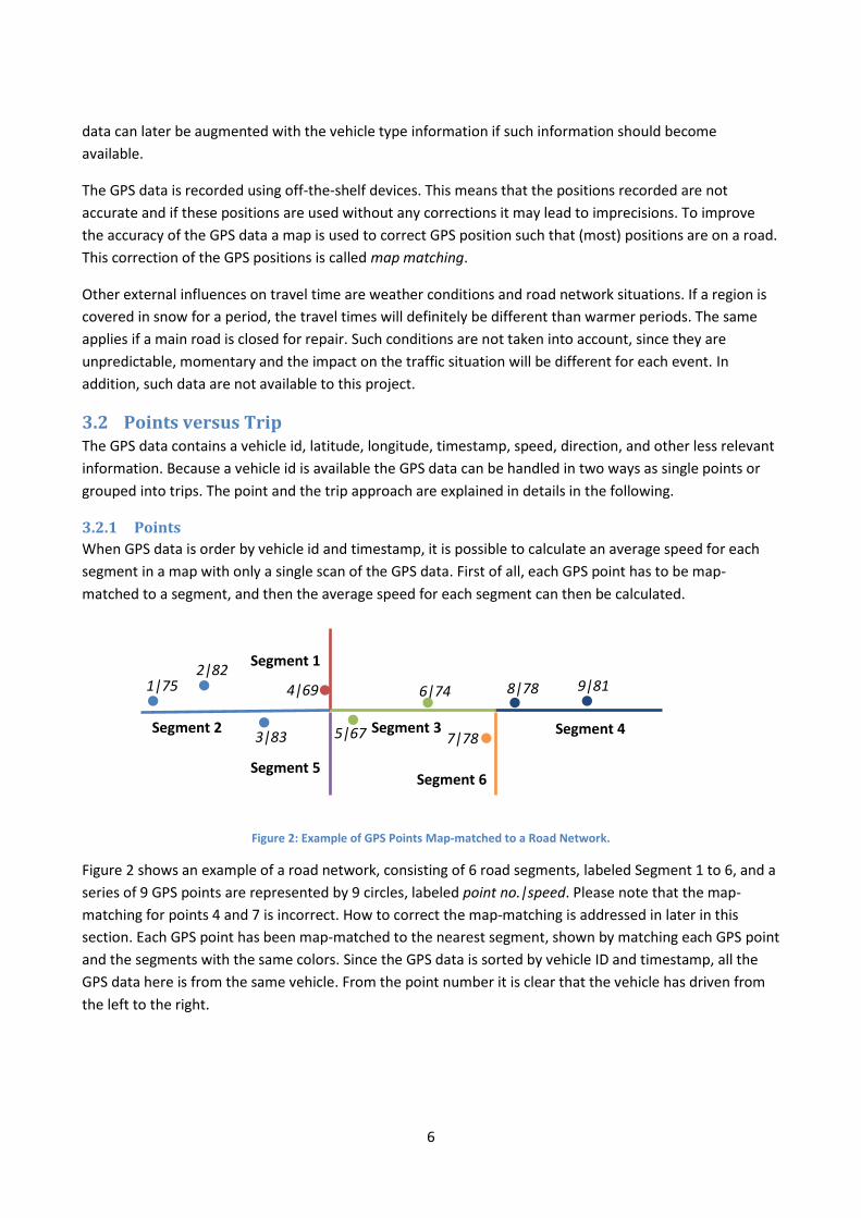
Figure 2 shows an example of a road network, consisting of 6 road segments, labeled Segment 1 to 6, and a

series of 9 GPS points are represented by 9 circles, labeled point no.|speed. Please note that the map-

matching for points 4 and 7 is incorrect. How to correct the map-matching is addressed in later in this

section. Each GPS point has been map-matched to the nearest segment, shown by matching each GPS point

and the segments with the same colors. Since the GPS data is sorted by vehicle ID and timestamp, all the

GPS data here is from the same vehicle. From the point number it is clear that the vehicle has driven from

the left to the right.

Segment 2

Segment 1

Segment 5

4|69

Segment 3 Segment 4

Segment 6

7|78 5|67

1|75 2|82

3|83

6|74 8|78 9|81

7

Segment Speeds Average speed Observations

1 69 69 1

2 75+82+83 80 3

3 67+74 70,5 2

4 78+81 79,5 2

5 - - 0

6 78 78 1

Table 1: Calculations of Average Speed for Each Segment

Table 1 shows how the average speeds are calculated from Figure 2. For each segment, the summation of

all the speeds is divided by then number of observations available for the segment, hence the average

speed for segment 1, for this vehicle, is (69) / 1 = 69, for segment 2 it is (75 + 82 + 83) / 3 = 80, and so on.

No observations exist on segment 5, thus no speed is stored for segment 5.

Figure 3: Example of Two Vehicles Driving the Same Segments at Different Speeds

The average speed for each segment is calculated on a per vehicle per segment passage basis and not on a

per GPS point basis, to eliminate the problem of a slow driving vehicle weighting more than a fast driving

vehicle. This problem is illustrated in Figure 3. Here two vehicles A and B cross three segments. Both

vehicles record their position each second. Vehicle A is driving slower than vehicle B. If calculating the

average speed for each segment from these GPS points, vehicle A will have higher influence on the average

speed than vehicle B.

Segment Calculation Observations Average speed

10 (41+43+42+45+44+83+85+86)/8 8 58.6

11 (43+44+47+44+46+40+43+86+89+91)/10 10 57.3

12 (43+42+39+37+38+93+95)/8 8 48.3

Table 2: Calculation of Average Speeds for Segment using GPS Points Directly

Table 2 shows the calculations for the average speed when not taken into account that the slower vehicle

has more points. For segment 10, the average speed is calculated to 58.6, and 8 observations have been

used for this average. The number of observations tells how many GPS points have been used for

computing the average speed. When looking at the number of observations in Figure 3, it becomes visible

that 5 of the 8 observations are recorded by vehicle A while only 3 of the 8 observations are recorded by

vehicle B. Thus, vehicle A’s average speed weights 62.5% (100 / 8 * 5), while vehicle B only weights 37.5%

(100 / 8 * 3). Hence, the slower a vehicle is driving on a segment the more observations will be available

and the higher the impact on the average will be.

41 43 42 45 44 43 44 47 44 46 40 43 43 42 39 37 38 Vehicle A x x x x x x x x x x x x x x x x x Vehicle B o o o o o o o o 83 85 86 86 89 91 93 95

Segment 10 Segment 12 Segment 11

8

Segment Vehicle Calculation Observations Average speed

10 A (41+43+42+45+44)/5 5 43.0

10 B (83+85+86)/3 3 84.6

10 Average (43+84.6)/2 2 63.8

11 A (43+44+47+44+46+40+43)/7 7 43.8

11 B (86+89+91)/3 3 88.6

11 Average (43.8+88.6)/2 2 66.2

12 A (43+42+39+37+38)/5 5 39.8

12 B (93+95)/8 2 94.0

12 Average (39.8+94)/2 2 66.9

Table 3: Calculation of Average Speeds for Segment with Concern to Segments Passed

To overcome this problem, an average speed for each time one vehicle has passed a segment must be

calculated. Table 3 shows an alternative way of calculating the average speeds. First an average is

calculated for each vehicle for each segment. Vehicle A’s average for segment 10 then becomes 43, while

vehicle B’s average becomes 84.6. When using these two values to calculated the average speed, the

weights now become even (50%/50%) for both vehicles, and the result of this is, that the average segment

speeds becomes faster, due to the higher weights of the faster car, vehicle B. This system, also eliminates

the problem with different recording frequencies would impact differently, due to more data from vehicles

with higher recording frequency.

When the average speed is known for a segment, it then is trivial to calculate the time it has taken to pass

the segment, due to the distance of the segment is known from the map.

Figure 4: Comparison constant speed and drastically acceleration

This method will also be usable if a vehicle suddenly accelerates drastically. Figure 4 shows two vehicles, C

and D, which both have the same recording frequency of 1 second. Both vehicles are passing the same

segment that is 100 meters long. Each vehicle has five GPS recordings marked with an x for vehicle C and an

o for vehicle D. The speed in meters pr. second (m/s) is shown above and below the GPS marks.

The average speed for vehicle C becomes ((20 + 20 + 20 + 20 + 20) / 5) = 20 m/s, while the average speed

for vehicle D becomes ((10 + 10 + 10 + 10 + 60) / 5) = 20 m/s. For vehicle D, the four 10 m/s speeds will

weight four times higher than the 60 m/s speed, and this is consider the most correct, because it is the

average speed that is wanted. Since GPS data is recorded with the same frequency, every GPS speed should

only weight 1/n, where n is the total number of speeds available.

20 20 20 20 20 Vehicle C x x x x x Vehicle D o o o o o 10 10 10 10 60

Segment 20, length=100

9

Figure 5: Problem with method and drastically acceleration

A problem arises though, if the drastically acceleration is not part of the segment, but leaps outside to the

next segment, as shown in Figure 5. Here the average speed of vehicle E would be calculated to ((10 + 10 +

10 + 10) / 4) = 10 m/s, because the drastically acceleration is not part of this segment. This problem cannot

be easily solved using the point-based approach. The trip-based approach described later does not have

this problem.

The point-based method has advantages and disadvantages. The main advantage is that all GPS data is

usable, if the data can be mapped to a road segment. Map-matching can be done in 70% of the cases, i.e.,

most GPS data can be used. This is also one of the disadvantages because no test can easily verify that the

GPS data is mapped to the correct segment. If we say that Figure 2 shows a trajectory of a vehicle driving

from the left to the right, it becomes clear that the method have some issues if the precision of the GPS

data is low. When following the trajectory, it seems like the vehicle is driving first on segment 2, then

segment 3, and at last segment 4. But due to inaccurate GPS points, one GPS point is mapped to segment 1

and another to segment 6. Another disadvantage is the fact, that when only using points it is uncertain

whether segments with ex. traffic lights will get an unfair low average speed due to many 0-speeds. Also a

problem exists when very drastically accelerations occur and the segment is as risk of missing this

acceleration, and the average speed becomes wrong. It is estimated that this problem is small and has very

limited influence on the travel times computed.

3.2.2 Trips

Instead of using the GPS data as points they could be treated as trips. A trip is defined as a series of GPS

data recorded while a vehicle has been driving from a source to a destination. When a trip is present, it is

possible to follow the exact route the vehicle has been driving. For GPS data to be handled as a trip, the

recording frequency must no more than 9 seconds between each GPS point. The 9 seconds are discussed in

Section 7.2.

Handling GPS data as trips requires a good map-matching algorithm. If a trip can be computed from a series

of GPS data from a single vehicle it can be calculated how long it has taken for this specific vehicle at a

specific trip to pass each road segment.

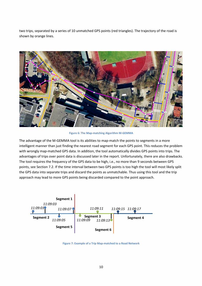
A map-matching algorithm and tool has been developed by (16). This tool excellence in dividing a series of

GPS data into trips and at the same time map-matching each GPS points to segments. An example on how

the tool works is showed on the map in Figure 6. A series of GPS data is shown as white arrows and the

path between each consecutive GPS point is shown by a purple line. Every GPS point is map-matched to the

most likely road segment, and the matching is shown by a blue offset line from the GPS point to the

matched segment. When no map-match exists a red warning triangle occurs above the white arrow. Each

time a GPS points cannot be map-matched, the trip is ended, and a new trip is started at the next GPS point

that can be map-matched. With this knowledge, it is clear from Figure 6 that the GPS points are divided into

Vehicle E o o o o o 10 10 10 10 70

Segment 20, length=100

10

two trips, separated by a series of 10 unmatched GPS points (red triangles). The trajectory of the road is

shown by orange lines.

Figure 6: The Map-matching Algorithm M-GEMMA

The advantage of the M-GEMMA tool is its abilities to map-match the points to segments in a more

intelligent manner than just finding the nearest road segment for each GPS point. This reduces the problem

with wrongly map-matched GPS data. In addition, the tool automatically divides GPS points into trips. The

advantages of trips over point data is discussed later in the report. Unfortunately, there are also drawbacks.

The tool requires the frequency of the GPS data to be high, i.e., no more than 9 seconds between GPS

points, see Section 7.2. If the time interval between two GPS points is too high the tool will most likely split

the GPS data into separate trips and discard the points as unmatchable. Thus using this tool and the trip

approach may lead to more GPS points being discarded compared to the point approach.

Figure 7: Example of a Trip Map-matched to a Road Network

11:09:07

Segment 2

Segment 1

Segment 5

Segment 3 Segment 4

Segment 6

11:09:13 11:09:09

11:09:01 11:09:03

11:09:05

11:09:11 11:09:15 11:09:17

11

When the tool’s map-matching is working correctly for a consecutive series of GPS data, it could result in a

series of data as shown by Figure 7. Here a GPS point is present with a frequency of 2 seconds and a

timestamp is shown for each GPS point along with a map-matching line between each GPS point and the

matched segment. Thus it is possible to calculate how long it takes to pass each segment on a trip by

subtracting the first timestamp for one segment with the first timestamp of the previous segment.

Segment This seg. first timestamp Next seg. first timestamp Duration

2 11:09:01 11:09:09 8

3 11:09:09 11:09:15 6

4 11:09:15 - -

Table 4: Calculation of Travel Time on a Segment

Table 4 shows an example for how long it has taken to pass two of the segments shown in Figure 7. For

segment 2, the timestamp of the first GPS point on the segment (11:09:01) is used as a basis for entering

the segment. The vehicle is then located on the segment until a new segment is entered, and the first

timestamp of the next segment (11:09:09) is the used as exit time of the segment. The duration between

these two timestamps is then the time it has taken to pass the segment, thus it has taken 8 seconds to pass

segment 2. The average speed driven on each segment can then be calculated, because the length of the

segment is recorded in the map.

Please note that the first and the last segment of a trip are not computed, while it is uncertain if a vehicle

has started or stopped in the middle of these segments.

The advantages of the trip method is the certainty of knowing that map-matching is most likely correct, and

when using GPS points with high frequency the can be read directly from the data and not estimated from

a set of GPS points. The lower the frequency of GPS points, the lower the precision of the duration

calculations get, due to more imprecise knowledge of when entering and exiting a segment. A disadvantage

of the trip method is the requirement of high frequency of the GPS points, to get stable and reliable trips. In

addition, the possible larger amount of discarded data can be an issue, in particular in areas with limited

GPS points available.

3.3 Data Foundation This section described the input data in details. First the GPS data is described. Second, map data is

described because a map is needed both to map-match the GPS data and to create the speed map. Third,

the requirements for computing the drive-time matrix are discussed. Finally, various challenges related to

the accuracy and correctness of the data sources is discussed.

3.3.1 GPS Data

To be able to use a GPS point it is necessary to have a unique vehicle ID for grouping data into trips. A

position is also crucial along with a timestamp for when the position was recorded. Speed and compass

direction is also very important, though can these manually be calculated if data is high frequency (few

seconds between recordings).

The GPS data provided, comes in the format shown in Table 5. Overall it contains data, which is available

from most GPS devices.

12

Variable Used Example Description

ID_GPSData 205574542 An unique id

VehicleId X 4705 An vehicle id

TXDatetime X 2010-11-21 08:09:51 Timestamp for recording of GPS data

RXDatetime X 2010-11-21 08:10:02.340000000 Timestamp for when server received data

LatDeg X 55 Latitude arc degree

LatMin X 45 Latitude arc minutes

LatFracMin X 7282 Latitude fraction of arc minutes

LongDeg X 8 Longitude arc degree

LongMin X 22 Longitude arc minutes

LongFracMin X 2128 Longitude fraction of arc minutes

Speed X 0 Speed in km/h

Course X 222 GPS compass course in degree

GPSStatus 8 A GPS status variable

IsStartMacro False Can define if a transport starts (unreliable)

IsStopMacro True Can define if a transport stops (unreliable)

MessageText R26 (0, 38648.9 km) A message bound to IsStart/StopMacro

AddDate 2010-11-21 08:11:01.343000000 Timestamp for adding data to database

Table 5: GPS Data Format

Three different kinds of timestamps are provided, though only the GPS recording timestamp, TXDatetime,

and the received data timestamp, RXDatetime, is interesting for this system. Using RXDatetime can help

verify the correctness of TXDatetime.

The GPS point is provided in latitude and longitude coordinates, and it is important to notice some features.

The latitude coordinate is positive on the northern hemisphere and negative on the southern.

The longitude coordinate is positive when located east of zero longitude and negative when west

of.

The coordinates are provided in the WGS 84 format (17). This defines the zero longitude to be

located 5.31 arc seconds east of Greenwich Prime Meridian.

The LatFracMin is a decimal of the LatMin and not a latitude arc second. For the example in Table 5

the correct notation of the latitude is 55° 45.7282’ E.

The LatFracMin is a four digit number, that means 42 is 0042, and when appending to the LatMin

45, the decimal value is 45,0042 and not 45,42.

Not all columns in the GPS point format are used by the system. All columns are documented to show what

is available.

3.3.1.1 Quality of GPS Data

The quality of the GPS data is determined by the frequency of how often GPS data is sampled. High quality

GPS data is data recorded with a frequency of at least one sample every 9 second. The 9 seconds has been

13

found by experiments, see Section 7.2. High quality GPS data can be used for trip map-matching because

the trip can fairly easy be recognized with high-frequency data.

Low quality GPS data is on the other hand data with more than 9 seconds between each GPS measure. Such

data cannot be used for trip map-matching while it can be used for point map-matching though.

3.3.2 Map Data

The map is retrieved from a spatially enabled database and contains all segments available in the road

network. A segment is a part of a road and a segment can only be joined with other segments in the ends.

Name Example Description

Segment id 615461 The identifier of the segment.

Road name Elm Street The name of the street that the segment is a part of.

Road category NE4 The category of the street.

Traffic direction BOTH Direction on segment; FORWARD, BACKWARD, or BOTH.

Segment location - An OGC line string describing the segment.

Segment start point 298219 An id of the join at the beginning of the segment.

Segment end point 298220 An id of the join at the end of the segment.

Length 100 The length of the segment in meters.

Forward speed limit 0 The sign posted speed limit (if available).

Table 6: Information Available of each Road Segment.

Table 6 describes the information available when a map is received from FlexDanmark. The information

showed is available for every segment and Figure 8 shows an example of a road network that is divided into

segments.

Figure 8: An Example of Dividing a Road Network into Segments

Every segment is built from a series of smaller lines, divided by the green dots. When a segment is joined

with other segments, the segment is ended with a purple larger dot. The segment in the black box in Figure

8 consists of 4 lines, labeled 1 to 4. The direction of the segment is very important. If traffic can travel only

from the left to the right, the direction is described as FORWARD. If the traffic can only travel from the right

14

to the left, the direction is described as BACKWARD. If the segment is built from the right to the left, with

green dot label 1 rightmost and the green dot label 4 leftmost, the FORWARD and BACKWARD are

reversed. If traffic can travel in both directions on the segment, the direction is described as BOTH.

As explained, segments can only be joined at the ends. The segment in the black box in Figure 8 is joined in

both connection point A and B, where A is the start point and B is the end point. Another segment is joined

with the segment’s start point, A, and this segments either have A as a start or end point. It is not required

that other segments join a segments start point or end point, e.g., if the segment is on a road with a dead

end.

3.3.2.1 Other Maps Sources

Besides the map received from FlexDanmark, the system has also been configured for using

OpenStreetMap maps (18). OpenStreetMap is a map created and updated by people around the world and

has the advantages that it can be used without paying license fees.

3.3.3 Points-of-Interest/Region Gravitation Points

To predict how long it takes to get from one region of a map to another, the map is divided into a number

of regions.

Figure 9: Example of a region with its Region Gravitation Point on a Map

An example of a region is shown in Figure 9. The black lines are the road network and the red lines are the

region’s borders. The red dot is the gravitation point of the regions, i.e., the point where the travel from all

direction into and out of the region is approximately the same. These points have been defined by domain

experts with in the transportation area.

Such points are called a point of interests (POIs). A region is defined by a name, the region’s boarders, and

the location of the POI. The regions make it possible to estimate travel-time in constant time by doing a

table look-up.

3.3.4 Data Challenges

In building the system there have been challenges with the consistence and reliability of the data. First of

all, duplicate data exists, which has to be taken into account. Duplicate means the same vehicle id has

Lat=56.22656 Long=10.1136

15

several data recordings at the same timestamp. Duplicates are eliminated in the ETL process, see Section

6.3.

Second, it happens that data is out of bound or is missing. Examples are that spatial coordinates are in the

middle or the sea or the speed of a vehicle is given as an empty string instead of an integer. Such typical

dirty data is eliminated in the ETL process.

Third, some GPS devices do not record the speed of the vehicle. Thus GPS points from these vehicles always

have 0 as speed. It is necessary to identify these vehicles to prevent these zero-speeds GPS points from

make the computed travel-times too low.

Finally, it happens that GPS points have timestamp many years into the future or the past. Such GPS points

are simply not used.

3.4 Peak versus Non-Peak Hours Peak hour is a term describing when the traffic congestion is higher than average. The time for when peak

hour occurs can be very different for different locations. FlexDanmark has manually defined peak periods,

which will be used by this system. The peak and non-peak periods used in this report are defined as follow.

Morning peak:

o Monday through Friday

07:30:00 to 08:14:59

Afternoon peak:


15:00:00 to 16:29:59

Peak:


07:30:00 to 08:14:59

15:00:00 to 16:29:59

Non-peak:


00:00:00 to 07:29:59

08:15:00 to 14:59:59

17:30:00 to 23:59:59

o Saturday and Sunday

00:00:00 to 23:59:59

The morning and afternoon peak hours are specializations of the general peak time, and weekends are

defined as non-peak time, because the traffic is different from working day traffic.

It is simple to alter the peak hours (and therefore also non-peak hours). The same peak hours are used for

all segments. Dealing with different peak hours for different segments is a major task that is considered

future research.

16

3.5 The Output Both the point and the trip calculations will result in two types of output. First of all a speed map of the

entire road network and secondly a drive-time matrix for how long it takes to get from one POI to another.

The speed map and the drive-time matrix are presented in details in the following.

3.5.1 Speed Map

A speed map is a table that contains the average speed on a segment for a given time period. The output

format used by FlexDanmark is shown in Table 7. Providing different output formats is simple.

Segment id Non-peak Peak

1 67 61

2 51 45

3 80 75

… … …

Table 7: Speed-Map Output Format

Segment id is the id of the segment, Non-peak is the speed for the segment at non-peak periods, while

Peak is the speed for the segment during peak periods. Multiple peak times can be provided, as shown by

Table 8, where additional Morning and Afternoon periods has been added. Periods can overlap, and in this

table, Peak is actually a weighted average from Morning and Afternoon periods. The possibility to have

overlapping periods has been requested by FlexDanmark because it is useful in the existing software stack

used.

Segment id Non-peak Peak Morning Afternoon

1 65 60 59 61

2 56 49 47 51

3 79 75 77 69

… … … … …

Table 8: Speed Map with Additional Columns for Detailed Peak Hours

The average speeds, which are provided in the speed maps, are calculated by finding the average speed for

each segment, during a given period, e.g., non-peak or peak.

3.5.2 Drive-Time Matrix

Finding the travel time by using a speed-map directly is time consuming. To speed-up estimating the travel

time between two points a drive-time matrix is used. The idea of such a drive-time matrix is that the

duration for how long it takes to get from one region to another is pre-calculated using region POIs, as

described in Section 3.3.3. Finding the travel time between regions is then a simple and fast lookup.

17

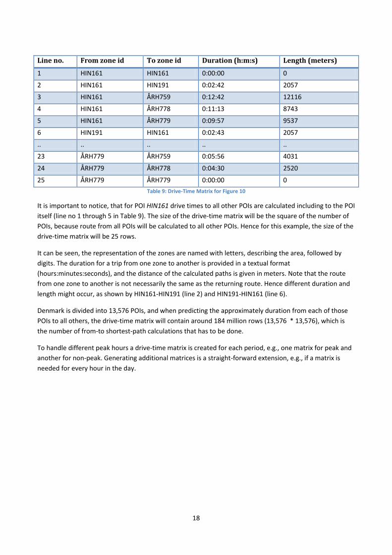
Figure 10: POIs of Regions near the City of Aarhus, Denmark

An example of a map is shown in Figure 10, with regions north of the city of Aarhus in Denmark. Five

regions (indicated blue rings) have been selected for illustrating how the drive-time matrix is used. The

fastest route from all POIs to all other POIs is pre-calculated and the output is shown in Table 9.

18

Line no. From zone id To zone id Duration (h:m:s) Length (meters)

1 HIN161 HIN161 0:00:00 0

2 HIN161 HIN191 0:02:42 2057

3 HIN161 ÅRH759 0:12:42 12116

4 HIN161 ÅRH778 0:11:13 8743

5 HIN161 ÅRH779 0:09:57 9537

6 HIN191 HIN161 0:02:43 2057

.. .. .. .. ..

23 ÅRH779 ÅRH759 0:05:56 4031

24 ÅRH779 ÅRH778 0:04:30 2520

25 ÅRH779 ÅRH779 0:00:00 0

Table 9: Drive-Time Matrix for Figure 10

It is important to notice, that for POI HIN161 drive times to all other POIs are calculated including to the POI

itself (line no 1 through 5 in Table 9). The size of the drive-time matrix will be the square of the number of

POIs, because route from all POIs will be calculated to all other POIs. Hence for this example, the size of the

drive-time matrix will be 25 rows.

It can be seen, the representation of the zones are named with letters, describing the area, followed by

digits. The duration for a trip from one zone to another is provided in a textual format

(hours:minutes:seconds), and the distance of the calculated paths is given in meters. Note that the route

from one zone to another is not necessarily the same as the returning route. Hence different duration and

length might occur, as shown by HIN161-HIN191 (line 2) and HIN191-HIN161 (line 6).

Denmark is divided into 13,576 POIs, and when predicting the approximately duration from each of those

POIs to all others, the drive-time matrix will contain around 184 million rows (13,576 * 13,576), which is

the number of from-to shortest-path calculations that has to be done.

To handle different peak hours a drive-time matrix is created for each period, e.g., one matrix for peak and

another for non-peak. Generating additional matrices is a straight-forward extension, e.g., if a matrix is

needed for every hour in the day.

19

4 Data-Warehouse Design In this section, the data-warehouse design will be discussed. For describing the data-warehouse schema,

some conventions are needed. The following describes the data type notations used through this section:

Smallint: A 2 byte value, ranging from -2^15 to 2^15.

Integer: A 4 byte value, ranging from -2^31 to 2^31.

Bigint: An 8 byte value, ranging -2^63 to 2^63.

Numeric (precision, scale): A value of precision number of digits with scale number of decimals,

e.g., 127.4 is a Numeric (4,1) and 1032.423 is a Numeric (7,3). A Numeric (3,1) ranges from -99.9 to

99.9.

Varchar: A string without length limits. Some DBMS might use Text instead.

Date: A date only, without time zone if nothing is defined.

Time: A time of day, without time zone if nothing is defined.

Timestamp: A date and time, without time zone if nothing is defined.

Boolean: A True/False value (without Unknown/null). Some DBMS might use a bit, a 1 byte tinyint

or other types to represent this value.

Geography: A spatial data type, storing geographic data, such as latitude, longitude, and altitude

coordinates. A Geography type can be seen as a restricted OGC Geometry type (19) (20), which only

allows coordinates in the Spatial References ID (SRID) 4326 and output measures are in meters.

PostGIS 2.0 has one such implementation, (21), while other OGC compliant DBMS’ should be able

capable of the same features using the OGC Geometry data type.

[FK]: When a data type is appended by [FK], it means it is a foreign key reference to another table.

This reference will be described in the description of the column.

The ordering of the table columns is unimportant, and can be manually defined if other sequences of

columns might be more optimal, e.g., for space preservation, Section 6.7.4.

First an overview of the design will be presented, along with a bus matrix describing relationships. Next the

different kinds of tables will be described in greater details.

4.1 Design The data warehouse is designed as a star schema, as shown in Figure 11. The tables are grouped by colors,

which determines their function and references between tables are show by lines.

20

Figure 11 Data Warehouse Star Schema

Dimension tables (blue and gray):

o All blue tables are dimensions. These tables contain dimensional data, which only rarely or

never changes.

o Gray tables are maps, and they differ a bit from other dimensions in the way, that the

number of map dimensions is dynamically and new maps can occur suddenly. Only one

map, Map, is shown as an example.

Fact table (green):

o The green table stores all data returned from the ETL and cleaning process. Only one table

exists for keeping all input data, namely Positioning Data.

21

Summary tables (yellow):

o The yellow tables store aggregated data, returned from map-matching algorithms. Two

kinds of tables exist, namely Point Map-matched Data and Trip Map-matched Data. Several

instances of these two tables might exist, while map-matched data for each Map will be

stored in different summary tables.

Reporting tables (red):

o Red tables contain output report from computed data from data warehouse. Two kinds of

reports exist, namely Speedmap and Matrix reports. Every time a new report is generated,

a new table is created.

All the tables are connected by references. The references can be seen in Figure 11 as pointing lines. The

references are colored as their source tables, for easier overview.

4.1.1 Bus matrix

One fact table exists in the data warehouse, along with two types of tables for storing summary data and

two types of tables for storing reports. Table 10 describes the Enterprise Bus Architecture Matrix (22) of the

data warehouse, where it can be seen which dimensions are used by which fact tables. Two dimensions,

namely Vehicle and Batch Load references other dimensions, hence they are also listed after the fact tables.

Dimensions Veh

icle

Ba

tch L

oa

d

Attrib

ute

Da

ta So

urce

Tim

e

Da

te

PO

I regio

ns

Ma

p

Positioning Data X X X X X X

Point Map-matched Data X X X X X X

Trip Map-matched Data X X X X X X

Speedmap X

Matrix X

Vehicle Dimension X

Batch Load Dimension X

Table 10: Enterprise Bus Architecture Matrix

In the following the fact tables and output tables are described in details.

4.2 Dimensions In total, the data warehouse has eight standard dimensions, which always exist, and an undefined number

of dimensions containing different maps, which appears when new maps are introduced.

4.2.1 Batch Load Dimension

The Batch Load Dimension stores description of every time data has been loaded into the data warehouse,

and keeps track of when data was processed and how long time it took. This can be seen from Table 11,

where every column is described. The Batch Load Dimension is a type 1 slowly changing dimension because

additional information to a batch load is stored in an existing row. Data is never overwritten in this table,

22

only added to empty columns. As an example, first the batchkey and sourcekey columns are inserted as a

new row. Later this row is updated with additional information, e.g., values for the etl_started and etl_done

columns.

Name Type Example Description

batchkey Integer 3 A surrogate key for referencing.

sourcekey Integer [FK] 4 Source key.

etl_started Timestamp 2012-04-11 12:01:05

Timestamp describing when ETL has started.

etl_done Timestamp 2012-04-11 12:06:12

Timestamp describing when ETL has finished.

cleaning_started Timestamp 2012-04-11 12:06:13

Timestamp describing when cleaning has started.

cleaning_done Timestamp 2012-04-11 12:10:45

Timestamp describing when cleaning has finished.

etl_rows_inserted Integer 2525243 Number of rows inserted into data warehouse by ETL.

description Varchar Data loaded from source 4

A textual description of the batch load.

Table 11: Batch Load Dimension

4.2.2 Data Source Dimension

Several GPS data sources can be used by the system, and the descriptions of these are saved in the Data

Source Dimension, shown by Table 12. The dimension makes sure different data sources can be identified,

and when loading data at ETL stage, the etl_plugin column describes what plugin should be used by ETL for

loading and parsing raw data. The values in the etl_plugin column are file names to python source code

that implements the ETL.


sourcekey Smallint 31 A surrogate key for referencing.

identifier Varchar flexdanmark_jylland A textual identifier of the data source.

description Varchar Flexdanmark vehicle data from Jutland

A description of the data source.

etl_plugin Varchar etl_fd_jylland_plugin A name of the plugin used for loading data.

Table 12: Data Source Dimension

4.2.3 Date Dimension

The Date Dimension contains the dates used in the data warehouse. The dimension is shown in Table 13

and is a dimension where the entries do not change when they first are created.

23


datekey Integer 20120425 A smart key (22) for referencing, [year, month, day].

date Date 2012-04-25 A SQL date type containing the date.

year Smallint 2012 The year.

month Smallint 4 The month.

days Smallint 25 The day of the month.

weekday Smallint 2 The weekday, 0-6, where first day, 0, in week is Monday.

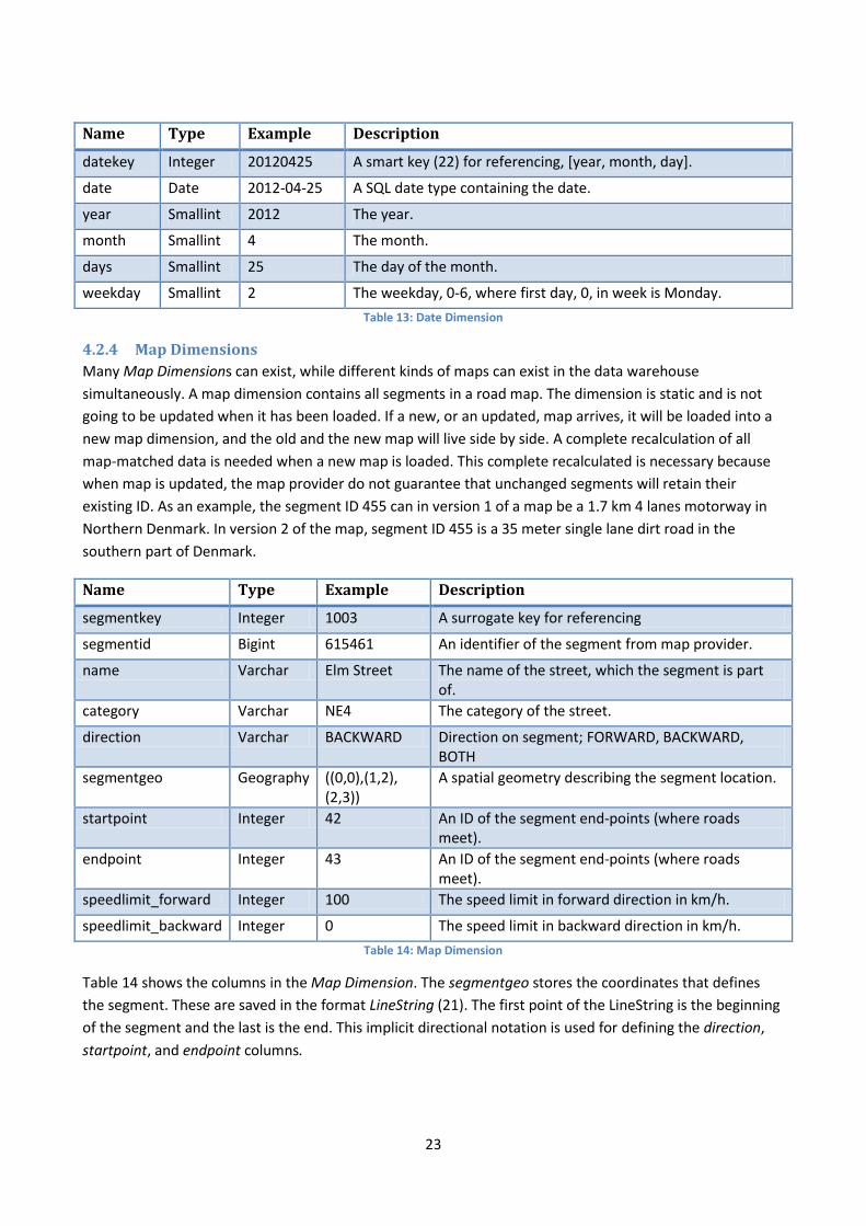
Table 13: Date Dimension

4.2.4 Map Dimensions

Many Map Dimensions can exist, while different kinds of maps can exist in the data warehouse

simultaneously. A map dimension contains all segments in a road map. The dimension is static and is not

going to be updated when it has been loaded. If a new, or an updated, map arrives, it will be loaded into a

new map dimension, and the old and the new map will live side by side. A complete recalculation of all

map-matched data is needed when a new map is loaded. This complete recalculated is necessary because

when map is updated, the map provider do not guarantee that unchanged segments will retain their

existing ID. As an example, the segment ID 455 can in version 1 of a map be a 1.7 km 4 lanes motorway in

Northern Denmark. In version 2 of the map, segment ID 455 is a 35 meter single lane dirt road in the

southern part of Denmark.


segmentkey Integer 1003 A surrogate key for referencing

segmentid Bigint 615461 An identifier of the segment from map provider.

name Varchar Elm Street The name of the street, which the segment is part of.

category Varchar NE4 The category of the street.

direction Varchar BACKWARD Direction on segment; FORWARD, BACKWARD, BOTH

segmentgeo Geography ((0,0),(1,2), (2,3))

A spatial geometry describing the segment location.

startpoint Integer 42 An ID of the segment end-points (where roads meet).

endpoint Integer 43 An ID of the segment end-points (where roads meet).

speedlimit_forward Integer 100 The speed limit in forward direction in km/h.

speedlimit_backward Integer 0 The speed limit in backward direction in km/h.

Table 14: Map Dimension

Table 14 shows the columns in the Map Dimension. The segmentgeo stores the coordinates that defines

the segment. These are saved in the format LineString (21). The first point of the LineString is the beginning

of the segment and the last is the end. This implicit directional notation is used for defining the direction,

startpoint, and endpoint columns.

24

The direction describes the allowed direction for traffic to drive on the segment. The variable can be

FORWARD for forward traffic only, BACKWARD for backward traffic only, or BOTH for traffic in both

directions.

The startpoint and endpoint columns are connection-id’s describing the how segments are connected. One

segment can only be attached to other segments at the start or end of the segment. It is not possible for

segments to be connected between the ends.

If the map is considered as a graph (from graph theory), all segments of the road network are edges in the

graph. All these edges are connected using nodes and each node has a connection-id. The startpoint and

endpoint numbers are ids of the node the segment is connected to in the graph. Now take a node, e.g.,

node number 42. All segments, which startpoint or endpoint is 42 are then connected to this node. That

means all number 42 of startpoint and endpoint are connected and traffic can be lead from one segment to

other via this node.

As a more practical example, let’s say three road segments meet in an intersection. This intersection can

have an id, say node number 47. The three segments connected to intersection 47 will have either their

startpoint or endpoint being 47, telling that these segments are connected at this point. No other

segments in the map are connected to intersection id 47 then. Whether it is the three segments startpoint

or endpoint that is 47 depends on the order of the coordinates in the segmentgeo column.

The speed limit of the segment, in both directions, is given in km/h.

Since a Map Dimension table will exist for every map present in the system, the tables will have different

names, such as “denmark_map”.

4.2.5 POI Region Dimension

The POI Region Dimension, shown in Table 15, keeps information of regions and their gravitaion point.

These regions are used when generating drive-time matrices. Except for id and name, two Geography

objects are stored. The first, point_geom, keeps a point, which is somewhere within the region_geom

region.


poikey Integer 4231 A surrogate key for referencing.

id Integer 238423 An id of the planet region

name Varchar CITY42 A name of the planet region

point_geom Geography (9.25, 11.24) The defined centrum point of the region

region_geom Geography ((9,11),(10,13), (9,9),(9,11))

The shape of the region.

Table 15: POI Region Dimension

4.2.6 Positioning Data Attribute Dimension

The Positioning Data Attribute Dimension, described by Table 16, keeps attribute information on each

single row. As can be seen from the table, except for the attributekey, the rest of the columns are Boolean

values, describing whether an attribute is applied to the observation or not. The attributes are stored so

true is good and false is bad. That means the optimal set of attributes for an observation is all true values.

25


attributekey Smallint 4 A surrogate key for referencing.

has_speeds Boolean False Does vehicle have speeds attached the observation?

is_unique Boolean True Is observation unique on timestamp and vehiclekey?

is_driving Boolean True Is vehicle driving or parked?

correct_timestamp Boolean True Is timestamp valid?

usable_for_point Boolean False Is observation usable for point map-matching?

usable_for_trip Boolean True Is observation usable for trip map-matching?

Table 16: Positioning Data Attribute Dimension

4.2.7 Time Dimension

The Time Dimension is a dimension that contains the timestamps of the data warehouse in local time

without timezone. The dimension is shown in Table 17, and it can be seen, that the precision is down to a

minute scale. No finer precision is needed, when aggregating data, hence seconds and milliseconds are not

a part of this dimension.


timekey Smallint 1420 A “smart” key (22) for referencing, [hour, minute, second].

time Time 14:20:00 An SQL time type.

hour Smallint 14 The hour.

minute Smallint 20 The minute.

Table 17: Time Dimension

4.2.8 Vehicle Dimension

The Vehicle Dimension is a dimension describing the details known about the vehicles. The dimension is

shown in Table 18. The vehicle details know is a vehicle ID given from the data source, and a description of

which source the vehicle comes from in sourcekey. Vehicles with similar IDs might occur from different

sources, hence it is necessary to have a reference to which source the id belongs to, when looking up a key

for a vehicle from a specific source.


vehiclekey Integer 495 A surrogate key for referencing.

vehicleid Varchar Taxi-2150 The vehicle id.

sourcekey Integer [FK] 31 A reference to a data source.

Table 18: Vehicle Dimension

4.3 Fact Table The single existing fact table will be described in this section, along with references to the corresponding

dimensions.

26

4.3.1 Positioning Data

The Positioning Data fact table stores all the positioning data after having performed ETL and cleaning on

those. A unique id for each entry exists along with foreign keys to seven dimensions referenced, see Table

19.

Seven measurements exist in the fact table. Sourcefile keeps a description of the source, from where the

data row has been read. This is useful for backtracking data, if any anomalies are encountered. The

sourcefile format is “full_path:line_number”, where full_path is an absolute path to the source file read,

and line_number is the line number where the data exists.

The column timestamp stores the timestamp of when the position was recorded, while the column

rx_timestamp stores the timestamp for, when data was retrieved by a data collecting system. The latter

timestamp, rx_timestamp, is useful for verifying the correctness of the first position timestamp, as

precision of this is unknown.

The speed column stores the recorded velocity in km/h and euclidean_speed is the computed velocity

between the previous position report and the current, by knowing the distance between the two

coordinates and the difference between the two timestamps.

The direction column holds the direction in degrees from north; hence the direction is a value ranging from

0 to 359 (if not invalid). The coordinate stores the position latitude and longitude (and altitude if available).


id Bigint 1024 An identifying id of the row.

datekey Integer [FK] 20120425 A foreign key to the Date Dimension.

timekey Smallint [FK] 1420 A foreign key to the Time Dimension.

vehiclekey Integer [FK] 495 A foreign key to the Vehicle Dimension.

sourcekey Smallint [FK] 31 A foreign key to the Data Source Dimension.

batchkey Integer [FK] 3 A foreign key to the Batch Load Dimension.

attributekey Smallint [FK] 4 A foreign key to the Positioning Data Attribute Dimension.

sourcefile Varchar /path/file1.csv:421 A text describing source file and line number of data, separated by “:”.

timestamp Timestamp with timezone

2012-04-25 14:20:41

Position record timestamp, with timezone.

rx_timestamp Timestamp with timezone

2012-04-25 14:21:13

Data collection timestamp, with timezone.

speed Smallint 42 Velocity in km/h.

euclidean_speed Integer 39 Euclidean velocity computed, in km/h.

direction Smallint 217 Direction in degrees from north.

coordinate Geography (9.2,11.5) Position data.

Table 19: Positioning Data Fact Table

27

4.4 Summary Tables The summary tables, storing aggregated data, will be described in this section. These tables contain map-

matched data.

4.4.1 Point Map-matched Data

This Point Map-matched Data table contains the computed average speed and duration for when each

vehicle has passed a segment and the data is not capable of being treated as a trip. Table 20 shows the

schema for the fact table. A unique id for each entry exists along with foreign keys to the six dimensions

used. The calculated values are the average speed of the vehicle when passing the segment along with the

time taken to pass the segment and the direction driven on the segment. One vehicle might have several

GPS recordings for the same segment while passing it. Thus the number of GPS rows used (number of facts

from Positioning Data table used) is stored in the numpoints column.


id Bigint 526 An identifying id of the row.


timekey Smallint [FK] 1420 A foreign key to the Time dimension.




segmentkey Integer [FK] 1003 A foreign key to a Map Dimension.

avgspeed Numeric(4,1) 36.1 The average speed of the vehicle while passing the segment.

seconds Numeric(4,1) 10.4 The calculated duration of passing the segment.

direction Varchar FORWARD Direction driven on segment.

numpoints int 3 The number of rows from Positioning Data used.

Table 20: The Point Map-matched Data Table

Since a Point Map-matched Data table will be created for every Map Dimension used for map-matching,

the name of the Point Map-matched Data tables will be appended by the map. Hence, a Point Map-

matched Data table could be named point_match_denmark_map for the map denmark_map.

4.4.2 Trip Map-matched Data

The Trip Map-matched Data table contains the computed average speed and duration for each segment

passed while a vehicle has been on a trip. The schema is shown in Table 21 and, besides of a unique

identifier, six foreign keys are referencing the related dimensions. To be able to identify each trip, a unique

number is assigned to each trip. In addition, the number of segments passed until this segment, on one

trip, is stored. Thus for each trip, the tripstep starts counting from 1 and increments with 1 for each

segment passed. The average speed and duration of passing the segment is saved too, along with the

number of rows from factgpsdata used.

28


id bigint 425 An identifying id of the row.


timekey Smallint [FK] 1420 A foreign key to the Time dimension.




segmentkey Integer [FK] 1003 A foreign key to a Map Dimension.

trip Integer 205 An id to distinguish different trips from each other.

tripstep Integer 18 A counter telling segment number of trip.

avgspeed Numeric(4,1) 36.24 The average speed of the vehicle while passing the segment.

seconds Numeric(4,1) 9.0 The calculated duration of passing the segment.

direction Varchar FORWARD Direction driven on segment.

numpoints Integer 3 The number of rows from Positioning Data used.

Table 21: The Trip Map-matched Data Table

Since a Trip Map-matched Data table will be created for every Map Dimension used for map-matching, the

name of the Trip Map-matched Data tables will be appended by the map. Hence, a Trip Map-matched Data

table could be named trip_match_denmark_map for the map denmark_map.

4.5 Reporting Tables The reporting tables are used for storing aggregated reports generated from the map-matched summary

tables. Two kinds of reporting tables exist, namely Speedmap storing speedmap data and Matrix, storing

drive time matrix data.

4.5.1 Speedmap

The Speedmap reporting table contains the outcome of a computed speed map, aggregated from a Point-

or Trip Map-matched Data table. The columns in the table are shown in Table 22. The speedmap is a one-

to-one relation to a Map Dimension. That means, for each segment of a Map, there will be one row in the

Speedmap table.

For each segment in the Speedmap, the will exist two columns for a number of periods. A period can be

every working day between 15.00 and 17.00 and for this period the average speed and number of

observations will be stored. Another period could be Fridays between 14.00 and 16.00. The number of

periods is variable and will be defined when computing the speed map.

29


segmentkey Integer [FK] 4847 The segment id.

period1_speed Numeric(4,1) 45 Average speed during one period

period1_obs Integer 7 Average number of observations during one period.

period2_speed Numeric(4,1) 41 Average speed during another period

period2_obs Integer 21 Average number of observations during another period.

… … … …

Table 22: The Speedmap table

Since the Speedmap table will be created every time a new speed map is made, the table name of the

speed map will be derived from the map-matched data table, the speed map is generated from along with

a timestamp of the speed map creation. A name will look like speedmap_{data source}_{date}_{time},

where {data source} is a map-matched data table and {date} could be 20120420, for the 20th of April 2012,

and {time} could be 141251 for the time 14:12:51.

If, e.g., a speedmap is generated from the Point Map-matched Data table point_match_denmark_map, the

speedmap could be named speedmap_point_match_denmark_map_20120420_141251.

4.5.2 Matrix

The reporting table Matrix contains the outcome of computing a drive-time matrix. The Matrix table, Table

23, references the POI Region Dimension twice. That is because the matrix stores distance and travel time

computed from all zones of POI Region Dimension (from_zone_pk) to all zones of POI Region Dimension

(to_zone_pk). Thus the size of the Matrix table will be the size of POI Region Dimensions squared.


from_zone_pk Integer [FK] 41 The zone id calculated from.

to_zone_pk Integer [FK] 79 The zone id calculated to.

duration Varchar 4:13:39 The travel time.

meters Integer 318163 The length of the route in meters.

Table 23 The Matrix table

Since the Matrix table will be created from a Speedmap table, but only from one column for one period

from the Speedmap table, the naming of a Matrix table looks like matrix_{short speedmap}_{period}, where

{short speedmap} is a speedmap table, without the “speedmap_” prefix. {period} is the period used from

the Speedmap.

If, e.g., a Matrix table is generated from the Speedmap table

speedmap_point_match_denmark_map_20120420_141251, for period2 data, the matrix table would be

named matrix_point_match_denmark_map_20120420_141251_period2.

30

5 Software Architecture The software architecture is a layered approach and is described in details in the following section. A non-

functional requirement on the software architecture is that it must consist mostly of open-source

components due to very expensive licenses for some of the commercial available components.

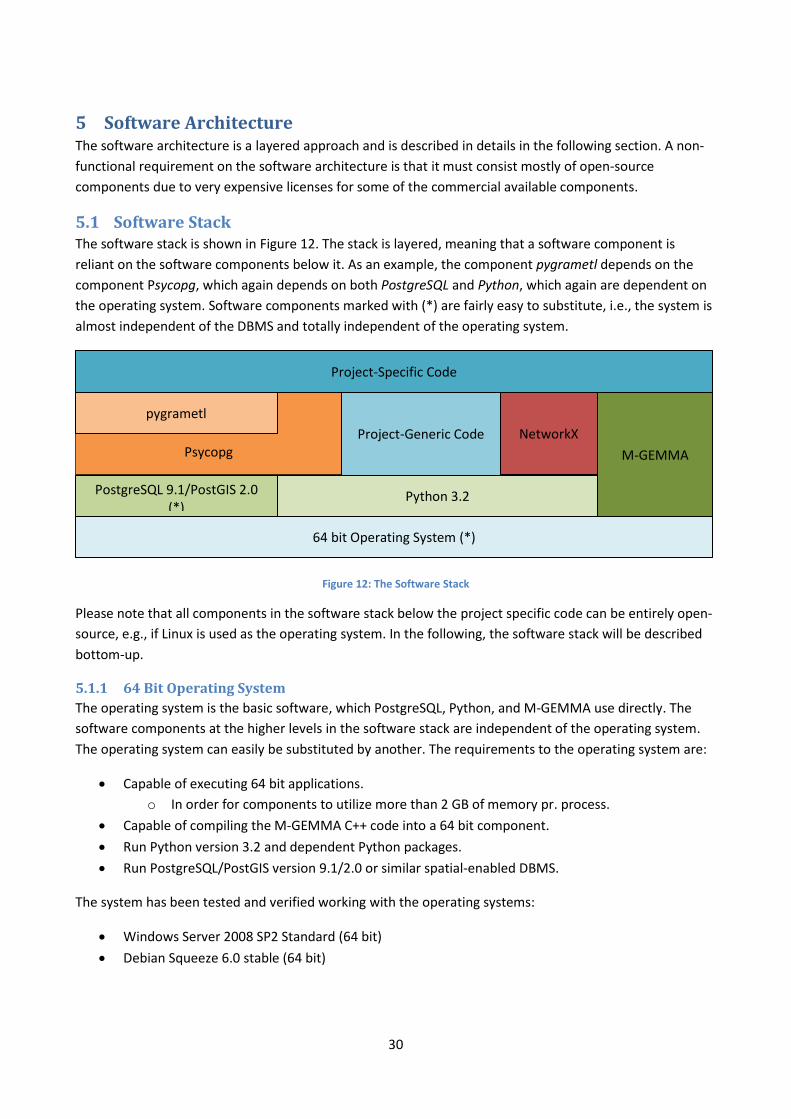
5.1 Software Stack The software stack is shown in Figure 12. The stack is layered, meaning that a software component is

reliant on the software components below it. As an example, the component pygrametl depends on the

component Psycopg, which again depends on both PostgreSQL and Python, which again are dependent on

the operating system. Software components marked with (*) are fairly easy to substitute, i.e., the system is

almost independent of the DBMS and totally independent of the operating system.

Figure 12: The Software Stack

Please note that all components in the software stack below the project specific code can be entirely open-

source, e.g., if Linux is used as the operating system. In the following, the software stack will be described

bottom-up.

5.1.1 64 Bit Operating System

The operating system is the basic software, which PostgreSQL, Python, and M-GEMMA use directly. The

software components at the higher levels in the software stack are independent of the operating system.

The operating system can easily be substituted by another. The requirements to the operating system are:

Capable of executing 64 bit applications.

o In order for components to utilize more than 2 GB of memory pr. process.

Capable of compiling the M-GEMMA C++ code into a 64 bit component.

Run Python version 3.2 and dependent Python packages.

Run PostgreSQL/PostGIS version 9.1/2.0 or similar spatial-enabled DBMS.

The system has been tested and verified working with the operating systems:

Windows Server 2008 SP2 Standard (64 bit)

Debian Squeeze 6.0 stable (64 bit)

Psycopg

64 bit Operating System (*)

PostgreSQL 9.1/PostGIS 2.0 (*)

M-GEMMA

Python 3.2

Project-Specific Code

NetworkX

pygrametl

Project-Generic Code

31

5.1.2 PostgreSQL 9.1/PostGIS 2.0

PostgreSQL (23) version 9.1 is the DBMS used. PostgreSQL’s spatial extension, PostGIS (24) is used to get

spatially functionality and makes it possible for storing spatial geometries. Also the tool PostGIS Shapefile

and DBF loader (21) is used to load maps in the Shapefile formats.

PostgreSQL can fairly easily be replaced by any spatially enabled DBMS that is OGC compliant. This would

require modifications to the project-specific code for parts concerning the DBMS such as connection

settings, bulk loading data, and creating and deleting indices and tables.

5.1.3 Python 3.2

Python (25) is used as the core programming language. Python 3.x is used, but this version requires changes

to some of the Python packages used in the software stack, which have not yet been ported to Python 3.x

On Linux (Debian) (26) Python is available through the package management system APT. The dependent

Python packages easily installs through the package management system APT or is compiled and installed

manually. On Windows the 64 bit version of Python is used.

5.1.4 M-GEMMA

M-GEMMA (16) is a third-party tool, used to map-match a sequence of GPS points to a road network, while

at the same time grouping the points into trips. M-GEMMA is implemented in C++ and does not depend on

any operating system specific libraries. The main memory usage of M-GEMMA depends on the size of the

map used. M-GEMMA is compiled into a 64 bit component to ensure that very large main-memories can be

used. In a 32 bit version M-GEMMA cannot handle a map of Denmark (approximately 600,000 segments) in

the address space available.

M-GEMMA requires the input GPS data to be in the NMEA format (27) that is a proprietary. However, the

format has been reverse-engineered (28) and NMEA is used.

The source code of M-GEMMA is slightly modified, in order to add functionality for parallel processing,

handling of maps, and additional input parameters. The original source code is available online (16). The

modifications to M-GEMMA are explained in Section 12.

5.1.4.1 M-GEMMA Non-Determinism

The output of M-GEMMA tool is non-deterministic, i.e., two runs of M-GEMMA on the same input can

return (slightly) different results.

It has been observed, that the last segment of a trip is not always included as part of a trip. That means, if

one run of M-GEMMA returns four segments as part of a trip, the next run might only return three

segments, while a third run might include the fourth segment again.

As an example, two runs of M-GEMMA, one the same map and same data set might return:

32

Run 1:

Route #0: filename

Paths

Score: 0 Avg: 0 Start: 10 Last: 13 Links: (10, 300000) (11, 300000) (12,

300015) (13, 300023)

Unmatched Info:

Start node: 0 End node: 9 Last Match: -1 Next Match: 10 Last Path: -1 Next

Path: 0

Start node: 14 End node: 20 Last Match: 13 Next Match: -1 Last Path: 0 Next

Path: 0

Run 2:

Route #0: filename

Paths


300015)

Unmatched Info:

Start node: 0 End node: 9 Last Match: -1 Next Match: 10 Last Path: -1 Next

Path: 0

Start node: 13 End node: 20 Last Match: 13 Next Match: -1 Last Path: 0 Next

Path: 0

For run 1, the output of M-GEMMA here states, that one trip is recognized as four data points, namely

point number 10 map-matched to segment 300000, 11 map-matched to segment 300000, 12 map-matched

to segment 300015, and 13 map-matched to segment 300023. The data nodes (GPS measurements) 0

through 9 and 14 through 20 are unmatched (cannot be map-match to the digital map used).

But when running M-GEMMA again (run 2) it states that a trip is recognized as only three points, namely

point number 10 map-matched to segment 300000, 11 map-matched to segment 300000, and 12 map-

matched to segment 300015. The point 13 is not recognized as part of a trip. The data nodes 0 through 9

are unmatched while data point 13 through 20 is unmatched.

This is no big issue, while it has only been observed that this happens for the last part of a trip, but it is very

important to take into account that the output is not predictable.

5.1.5 Psycopg

Psycopg (29) is a PostgreSQL database adapter for Python. The adapter can be exchanged with any other

adapter if a different spatial-enabled DBMS is used.

5.1.6 pygrametl

pygrametl (30) is a tool that makes easy to create ETL scripts in Python. It requires a database adapter for

communicating with a DBMS. Psycopg is chosen as the adapter in the software stack presented.

33

5.1.7 NetworkX

NetworkX (31) is a Python package that provides the ability of working with graphs and shortest paths

algorithms. The supplied algorithm used for shortest path is insufficient. Therefore an optimized shortest

path algorithm has been developed for handling bulks of shortest-path computations, see Section 13.

A NetworkX function is used to compute the shortest path from a single source to all other sources in a

graph, (32). The output of the algorithm is the distance to all other sources along with the paths to these.

There are some features that make the algorithm inefficient in the current setting.

1. It is unnecessary to return the paths to all the sources. NetworkX actually has a function only

returning the distance, (33).

2. This project requires both the shortest distance between the points and the actually length of the

path as output. This is not possible using the above algorithm.

To overcome these issues, a modified algorithm has been developed. This algorithm is based on the original

algorithm, with the ability of computing a second parameter when finding shortest paths. This second

parameter is used to return the distance of the shortest path. The details about the modified algorithm can

be found in Section 12.

5.1.8 Project-Generic Code

In the project, a number of Python modules are developed, e.g., for handling latitude and longitude

coordinates. These modules have not been available for the relative new Python 3.x programming

language. Such module is available for Python 2.x that is not fully upwards compatible with Python 3.x.

5.1.9 Project-Specific Code

On top of the software stack is the project specific code that depends solely on the software in the lower

layers. The project specific code is written entirely in Python and is partly optimized for multiprocessing.

The project specific code is discussed in details in the next section.

6 Implementation The following section describes the implementation in details. The focus is on the Extract, Transform, and

Load (ETL) process and how the implementation uses data parallel methods for scaling the system. The

code discussed in the section is the project specific code as shown in Figure 12.

6.1 Inter-Process Communication Before describing the individual modules, it must be introduced how data is sent between processes.

Python’s built-in multiprocessing package has a manager object (34) that can handle shared objects

between processes, i.e., inter-process communication (IPC).

The shared objects used in this implementation are Pythons first-in-first-out (FIFO) queues. A dedicated

process called the Manager handles locking of the shared objects to ensure correctness (34). This is

important when two or more processes are trying to modify a queue at the same time.

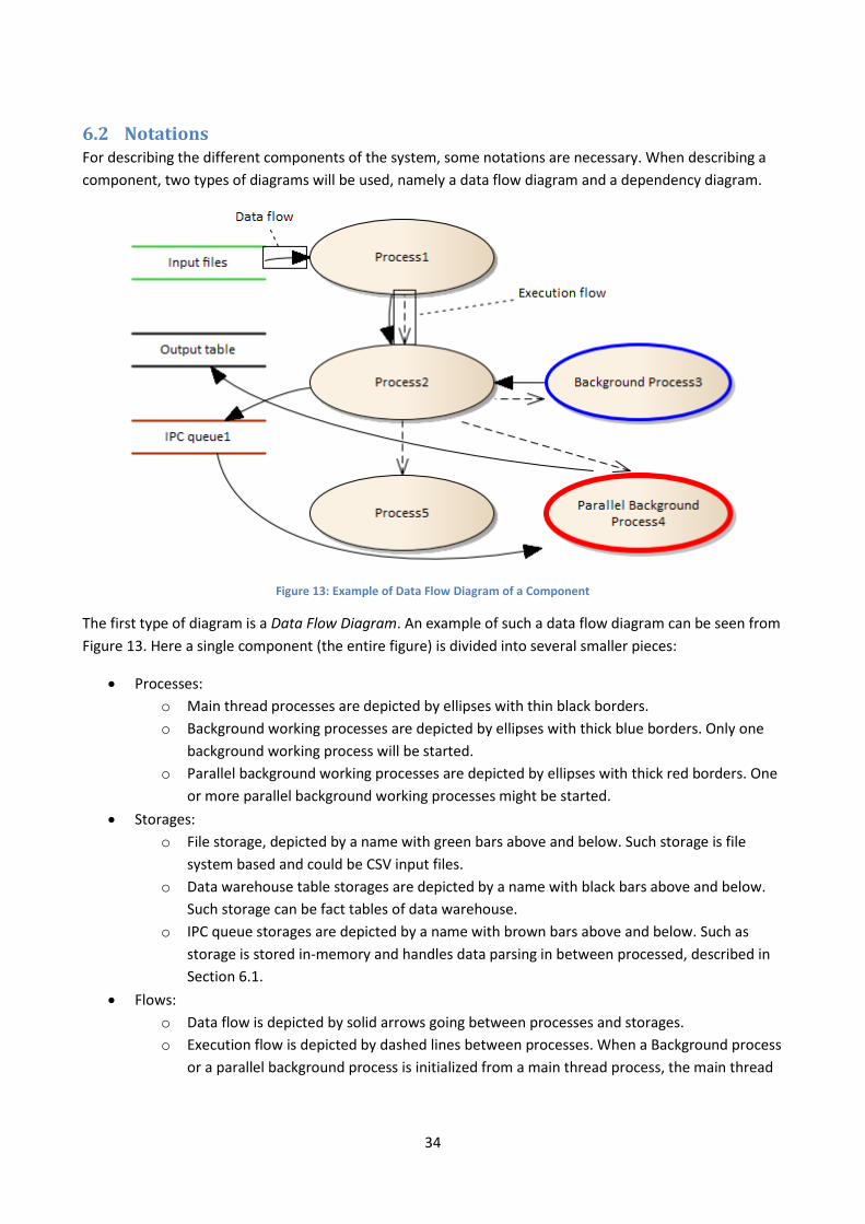
34

6.2 Notations For describing the different components of the system, some notations are necessary. When describing a

component, two types of diagrams will be used, namely a data flow diagram and a dependency diagram.

Figure 13: Example of Data Flow Diagram of a Component

The first type of diagram is a Data Flow Diagram. An example of such a data flow diagram can be seen from

Figure 13. Here a single component (the entire figure) is divided into several smaller pieces:

Processes:

o Main thread processes are depicted by ellipses with thin black borders.

o Background working processes are depicted by ellipses with thick blue borders. Only one

background working process will be started.

o Parallel background working processes are depicted by ellipses with thick red borders. One

or more parallel background working processes might be started.

Storages:

o File storage, depicted by a name with green bars above and below. Such storage is file

system based and could be CSV input files.

o Data warehouse table storages are depicted by a name with black bars above and below.

Such storage can be fact tables of data warehouse.

o IPC queue storages are depicted by a name with brown bars above and below. Such as

storage is stored in-memory and handles data parsing in between processed, described in

Section 6.1.

Flows:

o Data flow is depicted by solid arrows going between processes and storages.

o Execution flow is depicted by dashed lines between processes. When a Background process

or a parallel background process is initialized from a main thread process, the main thread

35

process will only continue to the next main thread process, when all background processes

has terminated.

The main thread processes are executed sequential; hence Process2 is not executed before Process1 has

finished. Because Process2 initialized background processes, here a single Background Process3 and

multiple parallel background processes Parallel Background Process4, the main thread will not continue to

Process5 from Process2, until the background processes and Process2 has finished.

The data flow of Figure 13 tells us, that data is loaded from an Input Table into Process1 and flows on to

Process2. From here one Background Process3 is initialized and will run in the background. Process2 will

receive data from Background Process3, though it will not send any data to Background Process3. Also

several background processes are executed in Parallel Background Process4. Data is not sent to Parallel

Background Process4 directly instead Process2 adds data to the IPC queue1 and Parallel Background

Process1 loads data from the IPC queue1.

The Parallel Background Process4 process contains a number of workers, which will compute data in

parallel and utilize multiple CPUs if available. Parallel Background Process4 sends data directly back to the

Output Table.

When both Background Process3 and Parallel Background Process4 has terminated, the main flow is ready

to move on to Process5.

Figure 14: Example of Component Dependency Diagram

The second type of diagram is a Component Dependency Diagram. Such a diagram can be seen from Figure

14, where external components are shown by rectangular boxes and their dependencies are shown. Two

kinds of dependencies exist:

36

A process can be dependent on an external component showed by a solid line between a process

and an external component. A process can utilize zero, one, or many different external

components. In Figure 14 Process2 uses both External Component2 and External Component3.

An external component can be dependent on another external component, shown by an

assembled line. In Figure 14 External Component2 is dependent on External Component1. This is

practically used by this system because the pygrametl package is making use of the Psycopg

package.

37

6.3 Extract-Transform-Load (ETL) The ETL is performed by a module constructed as shown by Figure 15. The ETL module is optimized for

parallelization and the coordination is handled by the Manager process.

Figure 15: Data Flow for ETL

From Figure 15 it can be seen, that ETL is a non-trivial process. Seven main processes are executed one by

one, and several of these have background workers, processing data in parallel. The ETL process can be

divided into two main parts. First data is loaded into a temporary table then data is loaded from the

temporary table, cleaned, and at last being loaded into the data warehouse.

38

Figure 16: Components used by ETL process.

Only two external components are used by the ETL process, namely pygrametl and Psycopg, as showed by

Figure 16. The pygrametl component is mainly used for loading data into data warehouse, due to its great

features for making it easy to bulk-loading data. Also it is used for handling dimensional integrity ensuranse

by lookups and ensuring existence of data in dimensions. When extracting data from the data warehouse,

e.g., in the Load Initialization process the Psycopg module is directly because the ETL functionality of the

pygrametl model is not needed.

39

6.3.1 Load Initialization

When the ETL module is started, a multiprocessing manager is started to handle the IPC. For every input

file, the path to the file is appended to the Input File Queue. An entry in the Batch Load Dimension is

created, while a new batch is started now.

A temporary fact table, Temporary Data Table, is created for storing loaded data. This is necessary, because

cleaning data requires data to be sorted by vehicle and timestamp, but data read from files are not

guaranteed to be sorted. This is a copy of the structure from the Position Data Partitions; see Section 4.3.1,

that contains all data.

6.3.2 Load Monitoring

The Load Monitoring process initializes n Parallel Data Load processes, where n equals the number of

available CPU cores. While the Parallel data load processes are working, this process waits for data to

become available in the Load status queue. If data becomes available, it is a message from a Parallel Data

Load process reporting its status.

6.3.3 Parallel Data Load

The Parallel Data Load processes all start out by adding a “STOP” entry to the Input File Queue. Then the

processes know when popping a “STOP” entry that no more input is available, and the process can stop.

A Parallel Data Load process starts out by popping a file path from the input queue and starts to read the

file one line at a time. First it is tested whether the line has the right format. Since datekey and timekey are

smart dimension keys, they are also calculated.

The vehiclekey needs to be looked up, and inserted if not existing. This is done by putting the vehicleid into

the Key Lookup Queue and waiting for a response on the Key Response Queue. The mapping from the

vehicleid to the vehiclekey is remembered by the Parallel Data Load process, and next time the vehicle is

met it is not necessary to look up the key.

Every valid line of data is added to the Temporary Data Table and all observed datekeys, and timekeys are

stored locally. When all files have been processed, all datekeys and timekeys will be added to the Key

Lookup Queue for ensuring existence of these keys. This cannot be done in parallel, while each Parallel Data

Load has its own database transaction, and race conditions might occur of two transactions tries to insert

the same value in a dimension at the same time. Note this is the case for the date, vehicle, and time

dimensions.

Every time an entire file has been processed, a status messages is put onto the command queue. The status

is a tuple, containing the size of the file just loaded, number of lines read from file, and number of lines

accepted as valid data.

6.3.4 Dimension Key Lookup

The Dimension Key Lookup process runs in the background and listens for items on the Key Lookup Queue

for ensuring dimensional consistency via pygrametl. If a vehicle ID is fetched, the corresponding vehiclekey

will be looked up in the Vehicle Dimension or inserted if not existing. The vehiclekey is returned via the Key

Response Queue and also stored locally for returning to main process when done.

40

If a datekey or timekey is fetched from the Key Lookup Queue the existence of this key is ensured in the

dimensions and stored locally too.

When meeting a “STOP” signal on the Key Lookup Queue the process stops, commits the changes to the

data warehouse and returns the vehiclekeys, datekeys, and timekeys to the main process.

6.3.5 Load Finalization

The Load Finalization starts two separate background processes Temporary Table Maintenance and

Duplicate Table Creation. These will be explained later. The last step in the Load Finalization process is to

vacuum and analyze the two tables created by the background processes such that the data is ready for

data cleaning. It is stored in the Batch Load Dimension that ETL load has finished.

6.3.6 Temporary Table Maintenance

Temporary Table Maintenance is a background process that creates a clustered index over the vehiclekey

and timekey columns. This means, all data is sorted physically by this index. This is important, because

when data is later to be loaded from this table it is loaded one vehicle at a time. The data can be

automatically loaded in sorted order due to the clustered index. Experiments showed that if the table is

non-clustered the loading is much slower.

6.3.7 Duplicate Table Creation

The Duplicate Table Creation process creates a table that will be used to determine, if duplicate exists when

comparing existing data warehouse with newly loaded data.

This could be done by comparing every row of the Temporary Data Table with the Position Data Partitions,

when performing cleaning. This do unfortunately introduce an overhead, especially because when cleaning

data and loading it into Position Data Partitions, the indices and references of Position Data Partitions is

dropped for performance improvements of bulk load.

Thus a Temporary Duplicate Check Table is created from the existing Positioning Data Table. Testing for

duplicates uses the two columns vehiclekey and timestamp, and of performance reasons these two

columns are combined into one column of type numeric(19,3). This is done by appending vehiclekey to the

Unix timestamp of timestamp. The three digits of the numeric is to make sure eventually milliseconds are

included and while a Unix timestamp takes 10 digits (plus up to 3 decimals), and with 19 available digits,

there is room for 999,999 different vehicles. The numeric value can easily be expanded to contain even

more vehiclekeys.

To optimize the Temporary Duplicate Check Table, only vehiclekeys and datekeys that exist in the

Temporary Data Table will be loaded from the Position Data Partitions, and vehicles and dates not

observed in the new batch will not be considered as possible duplicates, hence they are not stored in the

Temporary Duplicate Check Table.

6.3.8 Cleaning Initialization

First it is stored in the Batch Load Dimension that cleaning has started. Then when the data is ready for

cleaning, the Positioning Data Table needs to be prepared. This table is partitioned horizontally where each

partition holds a range of vehiclekeys for one year of data, see Section 6.7.1 for more details.

41

The partitions are prepared for receiving data by dropping indexes and foreign-key references. Only

partitions where data is added have their indexes and foreign keys dropped. The drops are done of

efficiency reasons.

If a partition does not exist, it is automatically created. Autovacuum in PostgreSQL is disabled on all

partitions that will be receiving data. This disabling is done because the autovacuum process can start at a

random time, which is a waste of resources because other processes later might append to the partition

again. Hence vacuuming and cleaning is performed manually afterwards.

All unique vehiclekeys from the Temporary Data Table will be loaded and added to the Vehicle Cleaning

Queue for later parallel processing.

6.3.9 Cleaning Monitoring

The Cleaning Monitoring process starts n Parallel Data Cleaning processes. n equals the number of CPU

cores available for the system. While these processes are running, this process will receive status reports

from the Cleaning Status Queue.

6.3.10 Parallel Data Cleaning

The Parallel Data Cleaning process is several parallel processes that help determining several kinds of

characteristics of the data. First a “STOP” signal is put into the Vehicle Cleaning Queue, for the process to

know when to stop. Until a “STOP” signal is met, vehiclekeys will be loaded from the Vehicle Cleaning

Queue and for every vehiclekey, data is loaded from the Temporary Data Table, order by the timestamp of

the row. When loading data from the Temporary Data Table it is verified if a similar row exists in the

Positioning Data Partitions, using the Temporary Duplicate Check Table for faster lookups.

For every row it is computed what partition of the Positioning Data Partitions the data should be stored

into. The Euclidean distance is computed between the previous and the current row, and if no speed or

compass direction is stored with the data, these are added if the duration between the previous and the

current row is no more than three seconds. Within three seconds, the accuracy of computing speed from

measurements is considered acceptable. This can make data with no speed usable for the system, if only

they are recorded with up to maximum of three seconds between each row.

Every row of data has a set of attributes. These attributes, Section 4.2.6, are determined using the test

cases of the following sections. When all attributes has been set, the data will be inserted into the correct

partitions.

When it can be determined that a range of partitions will no longer be used for inserting data, these

partitions will be committed to the data warehouse. This can be done, because vehiclekeys are processed in

sorted order, and vehiclekey is one of the columns the Position Data Partitions is partitioned over. If this is

not being done, there is a risk of having thousands of tables with bulk data waiting to be loaded and

committed, which might take up a lot of disk space.

Some assurances of the data quality will be performed, and attributes will be added to each data row, for

determine usability of this row. The attributes are introduced and discussed in Section 4.2.6 and the

following will describe when the requirement of each attribute is met.

42

6.3.10.1 Vehicle has Speeds

Some vehicles are known not to report speeds with their data. This is identified by checking if either the

previous row has speeds or if the previous row knows of rows before having reported speeds previously, or

if the speed of the current row is more than 0. When one row has observed a speed, this knowledge will be

automatically inherited to all the following rows of a vehicle. If vehicle do record speeds, the has_speeds

attribute is true.

6.3.10.2 Row is Unique

Whether a row is unique or not, is determined by two factors:

Comparing to existing data in Position Data Partitions (using the generated Temporary Duplicate

Check Table).

Comparing to other rows in the current batch from the Temporary Data Table.

Comparing to the existing data is performed when loading data from the Temporary Data Table. At this

moment, it is checked if any entry exists of the Temporary Duplicate Table that equals the current row on

vehiclekey (not vehicleid) and timestamp.

Comparing to other rows of the new data can be done by comparing the current row to the previous row

read. This can be done because data is sorted by timestamp when loaded and if two or more equal

timestamps exists in the Temporary Data Table for a vehiclekey, they will occur after each other.

If no duplicate row exists, the is_unique attribute of the current row is set to true.

6.3.10.3 Parked versus Driving

Determines whether a vehicle is driving or is parked is a challenging task. If a vehicle has not moved more

than 50 meters within the last 120 seconds it is said to be parked, if at least three observations are present.

If the vehicle has moved more than 50 meters it is known to be driving and if not three observations are

available it is unknown whether the vehicle is parked or moving, hence it is said to be moving.

If a vehicle is driving, the is_driving attributes is set to true.

6.3.10.4 Correct Timestamp

It is determined if vehicle has reported a correct timestamp by comparing the timestamp to the

rx_timestamp timestamps of the data. The rx_timestamp value describes when data was received by a data

storage service.

For data to be valid, they have to be sent within 1 hour back in time, from when it was received, and only

up to 15 minutes into the future. If data is sent more than 1 hour back, it cannot be verified if data is

transmitted late or the logging equipment has a faulty timestamp. Logging equipment should not have

timestamps in the future, while they are though allowed to report timestamps up to 15 minutes into the

future as a buffer.

If timestamp is correct, the correct_timestamp attribute is set to true.

43

6.3.10.5 Row is Usable for Point

For a row to be usable for point map-matching, the Correct Timestamp, Vehicle is Driving, Vehicle Has

Speeds, and Row is unique attributes must all be true.

If they true, the usable_for_point attribute is set to true.

6.3.10.6 Row is Usable for Trip

For a row to be usable for trip map-matching, the attributes is_unique and correct_timestamp must be

true. It is also tested, if there exists 10 rows of data from the same vehicle, with up to maximum 9 seconds

between each data row. The requirements minimum of 10 rows with maximal 9 seconds between each is

needed to ensure that the M-GEMMA tool is able to map-match the data as a trip. These requirements are

not listed in the M-GEMMA documentation but found via extensive testing of the tool. Further, M-GEMMA

is a CPU and memory intensive tool to deploy, hence the more data that can be sorted out as not usable,

the faster M-GEMMA will perform.

If data might be usable for trip map-matching, the usable_for_trip attribute will be true.

6.3.11 Partition Maintenance

When data is cleaned and loaded into Position Data Partitions, these partitions needs to be maintained.

This is done by the Partition Maintenance process. This process starts by generating references for all

partitions. This cannot be performed in parallel due to every reference creation uses locks that prevents

this to be processed in parallel.

After this has happened, every partition is added to the Partition List Queue and n Partition Index Creation

processes are started, where n equals the number of CPUs.

6.3.12 Partition Index Creation

The Partition Index Creation runs in parallel and starts by creating an index over the vehiclekey and

timestamp columns. Afterwards the each partition is clustered on this index, to make data sorted on disk.

This speeds up loading data when later querying for these again, while more sequential reads will be

performed and less random reads. Next indexes are created on columns and autovacuum is enabled.

This is done for every partition in the Partition List Queue. First though, a “STOP” signal is put into the

Partition List Queue, to let the process know when no more data is present.

6.3.13 Cleaning Finalization

Finally, it is stored in the Batch Load Dimension that cleaning has finalized.

6.4 Generating Points and Trips The generation of point map-matched data and generation of trip map-matched data are two separate

steps that are combined into a single process. This because generating trip map-matched data might not

fully utilize the number of CPUs of the system and then point map-matching can utilize the spare CPU

power.

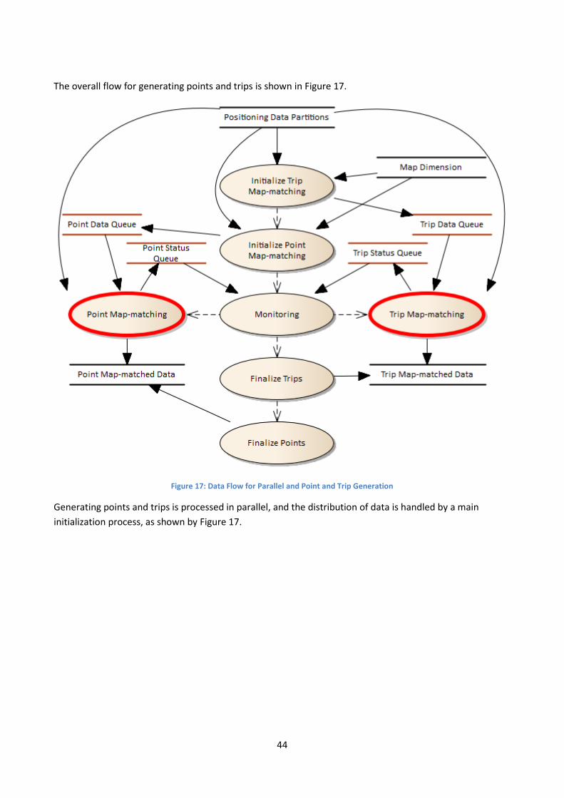
44

The overall flow for generating points and trips is shown in Figure 17.

Figure 17: Data Flow for Parallel and Point and Trip Generation

Generating points and trips is processed in parallel, and the distribution of data is handled by a main

initialization process, as shown by Figure 17.

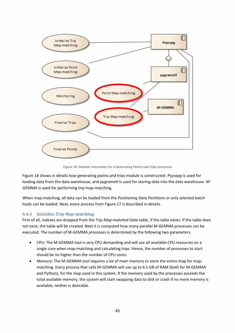
45

Figure 18: Module Interaction for a Generating Points and Trips processes

Figure 18 shows in details how generating points and trips module is constructed. Psycopg is used for

loading data from the data warehouse, and pygrametl is used for storing data into the data warehouse. M-

GEMMA is used for performing trip map-matching.

When map-matching, all data can be loaded from the Positioning Data Partitions or only selected batch

loads can be loaded. Next, every process from Figure 17 is described in details.

6.4.1 Initialize Trip Map-matching

First of all, indexes are dropped from the Trip Map-matched Data table, if the table exists. If the table does

not exist, the table will be created. Next it is computed how many parallel M-GEMMA processes can be

executed. The number of M-GEMMA processes is determined by the following two parameters.

CPU: The M-GEMMA tool is very CPU demanding and will use all available CPU resources on a

single core when map-matching and calculating trips. Hence, the number of processes to start

should be no higher than the number of CPU cores.

Memory: The M-GEMMA tool requires a lot of main memory to store the entire map for map-

matching. Every process that calls M-GEMMA will use up to 6.5 GB of RAM (both for M-GEMMA

and Python), for the map used in this system. If the memory used by the processes exceeds the

total available memory, the system will start swapping data to disk or crash if no more memory is

available, neither is desirable.

46

The number of Trip Map-matching processes that will be started is defined to be the smallest parameter of

the number of CPU cores available and the total GB of memory divided by 6.5 (due to M-GEMMA takes

roughly 6.5 GB of main memory, explained above). With the hardware available to the project 3 processes

are started, see Section 7.

To balance the work between the processes, data for the vehicles are split into a number of runs that

ensures that it highly unlikely that one or a few of the processes need to do all the trip map-matching. The

work load is not split on a per vehicle basis because it is too expensive to start the M-GEMMA process for

all vehicles, because it loads the entire map every time. The load balance tries to balance between large

runs and even fair load balancing. Data that can be trip map-matched is divided into batch loads, containing

a range of vehiclekeys to be map-matched at a time. Data is loaded from the Positioning Data Partitions to

the Trip Data Queue, for rows where the usable_for_trip attribute is true, and the vehicle key is within the

range of vehiclekeys currently being processed.

A map for M-GEMMA is generated from the segment dimension in the data warehouse. This map only

changes if the segment dimension has changed. This is a simple task and is therefore always done to ensure

an up-to-date map.

6.4.2 Initialize Point Map-matching

For point data, indexes and references are dropped from the Point Map-matched Data table, if the table

exists. If not, the table will be created.

Data to be point map-matched is being loaded from the Position Data Partitions, where the attribute

usable_for_point is true. Data is added to the Point Data Queue and one vehiclekey is added at a time,

hence one vehiclekey will be processed at a time.

A map is initialized from the Map Dimension, for making it possible to determine direction on segments.

6.4.3 Monitoring

The Monitoring process starts by initializing the Trip Map-matching and Point Map-matching background

processes. Up to 3 Trip Map-matching processes can be initialized (due to memory restrictions, explained

above), and for the remaining CPU cores, Point Map-matching processes can be started because these

processes only require limited main-memory resources.

The Monitoring process will keep track of progress of the background processes, and when a Trip Map-

matching processes has finished another Point Map-matching process might be started, if more data is

available. Status reports are received through the Point Status Queue and the Trip Status Queue.

6.4.4 Trip Map-matching

Data for M-GEMMA is stored in the fixed file format accepted by M-GEMMA. This fixed format uses

different units, e.g., for position, time, and speed than those stored in the data warehouse. As an example,

the unit for speed is knots instead of km/h.

To be able to load the trip output from M-GEMMA into the data warehouse a second file is generated that

contains information that makes it possible to join the M-GEMMA output with the data stored in the data

warehouse.

47

For every range of vehiclekeys loaded from Trip Data Queue, data is read from the Positioning Data

Partitions and converted to M-GEMMA data files.

Next, M-GEMMA is started as a background process, and the output is piped into Generate Trip Data

Process. The data is piped, because the M-GEMMA process and the Python process are totally separated

applications, and the only output from M-GEMMA is printed to console, which is intercepted by Python

using a pipe.

A unique, sequential number is assigned to each trip. Hence the maximum existing value of the trip column

in the facttripdata table is retrieved.

M-GEMMA outputs a string message for each trip generated and for status information. Two types of string

messages are used 1) when a new vehicle ID is found in the input file and 2) when a trip has been

identified. These two types of output are discussed in the following.

The M-GEMMA output for when a new vehicle is recognized looks like (including the starting white spaces):

Route #0: nmea_127_1

The output variable Route #0 describes that this is the first file loaded and the filename of the input data

is nmea_127_1, with extension .txt. The file name describes, that the data is in NMEA format, the

vehicle id is 127, and this is file number 1. Every time a new vehicle ID is recognized, the corresponding data

file is read to be able to restore the M-GEMMA output with usable data into the data warehouse.

The M-GEMMA output for a recognized trip looks like the following.


300015) (13, 300023)

The Score: 0 and Avg: 0 values are always 0, while the Start and Last variables describes the

number of the first and last GPS point used for this trip. It is visible that this trip spans over 4 GPS points, 10

through 13. Afterwards a segment mapping for every GPS point is described in the format (GPS no.,

segment on line number). It can then be seen the GPS point 10 and 11 are located on the segment in line

number 300,000, GPS point 12 is located on segment 300,015, and GPS point 13 is located on segment

300,023. All this information is returned to the Generate Trip Data process.

Every time a trip is returned by M-GEMMA, the duration for passing each segment is calculated. The

duration is calculated as the timestamp of the first point on the segment with the timestamp of the first

point on the next segment. Hence, for the example above, the duration would be:

(timestamp of line 12) - (timestamp of line 10) = duration for passing segment 300,000

The direction driven on the segment is determined by comparing the first position on next segment

(position of line 12) with the current segment. If the position is closest to the end point of the segment, the

direction is most likely “FORWARD”, while if the position is closest to the start point of the segment, the

direction is most likely “BACKWARD”.

48

Every time a new line with a trip is outputted by M-GEMMA, the variable describing the trip number is

incremented by one, and every segment used on a trip is also assigned an incremental segment number

from 1 to the number of segments in the trip. These numbers are used for keeping track of all trips. The

average speed of a vehicle is calculated for the segment too, by using the length of the segment from the

segment dimension. At last the data is added to the Trip Map-matched Data table, aggregated to one entry

for each segment passed.

6.4.5 Point Map-matching

Generating the point data is done by map-matching the position to the digital map. If one or more segment

exists within 50 meters from the location, the nearest segment is picked. If no segment exists, the data is

discarded.

This is done by letting PostGIS find the nearest segment when loading data. This is implemented by using

the PostGIS function ST_DWithin(segment, position, distance) that returns all segments within distance

(given in meters, when using Geography data type) of position. Then the returned segments can be ordered

by ST_Distance(segment, position), and the first entry will be the nearest. ST_Distance will not make use of

spatial index hence the ST_DWithin is performed first which do utilize index.

To ensure that slow moving vehicles does not weight higher than fast moving vehicles, a vehicle must only

weight by one every time it has been on a segment, see Figure 3. This is implemented by testing if the

vehicle at the previous row position was positioned on the same segment as the current position within a

timeframe of 15 minutes (can be configured). 15 minutes is chosen because, some vehicles do only very

seldom record GPS updates. If a vehicle is still on the same segment, the average speed of the GPS points

can be calculated. This continues until the vehicle is on another segment or the time frame is exceeded. At

this point, the average speed of the vehicle on the segment can be computed and stored into the Point

Map-matched Data table.

The duration for passing the segment is also calculated. This can be done because the length of segments

can be fetched from the Map Dimension using ST_Length (returns distance in meters, when using

Geography data type). If the average speed on the segment is 0 km/h it is rounded up to 1 km/h to avoid

modeling that a vehicle uses infinite long time to pass a segment. An average of 0 km/h on a segment can

occur if a vehicle only has a few position points on a segment due to the segment is short or the position

points are infrequently received, e.g., every 60 seconds.

Direction is computed on a segment by comparing the compass direction to the direction of the sub-

segment of a segment which is closest to the point.

6.4.6 Finalize Trips

When trips have finished being computes, references and indices will be created on the Trip Map-matched

Data table, and the table will be physically ordered on disk, according to vehiclekey and datekey to improve

sequential reads when later reading out data. The remaining M-GEMMA data files are deleted.

6.4.7 Finalize Points

When trips have finished being computes, references and indices will be created on the Point Map-

matched Data table. The table will be physically ordered on disk, sorted by vehiclekey and datekey for

improving sequential reads when data are read later.

49

6.5 Computing Speed Maps After having finished the map-matching and loaded data into the data warehouse, the next step is the

generation of speed maps.

A speed map is an aggregation over map-matched data, grouped per segment of Map Dimension. It is

possible to set requirements to speed map generation:

Request a minimum number of observations on a segment.

Request a time frame for what data should be used, e.g., only for the last year.

Request that computed speed on segment is no higher than allowed speed on segment.

Request a minimum speed on segment, to ensure no segments will have extremely slow speeds.

Figure 19: Data Flow for Generating Speed Maps.

The data flow can be seen from Figure 19. First all segments of Map Dimension is loaded and added to the

Segment Input Queue. Then averages are computed by Preload Segments Averages, which will be used if

not enough observations is available on a segment. Each segment is processed by a number of parallel

workers, the Compute Speedmap processes, handles by the Monitoring process, which compute the

average speeds on a segment and outputs to the Speedmap Table if enough observations are met. If not,

the average speed will be used instead, earlier computed. These segments with average speeds will have

the average speed of similar segments attached. Finally, the speed map is outputted to Speedmap File

Output and the speed map is ready for usage in other systems.

50

Figure 20: Components Used by Computing Speed Maps

Figure 20 shows the component dependencies of the Computing Speed Maps task. Psycopg is used when

loading data from the data warehouse (ETL functionality not required), while pygrametl is used for inserting

data (ETL functionality required).

6.5.1 Initialization

The Initialization process creates a table for storing the speed map. It also loads all segments from the Map

Dimension and puts the segmentkeys onto the Segment Input Queue.

6.5.2 Preload Segment Averages

If requirements for minimum number of observations are set, then the Preload Segment Averages process

will load the averages for each category of segments. A category is defined by the Map Dimensions

Category attribute, and similar segments are grouped into one average. This is done for each period of data

to be processed, e.g. peak and non-peak hours. If time restrictions is set on, how for back data should be

used, this restriction will be kept when loading data for averages.

6.5.3 Monitoring

The monitoring process keeps track of the parallel Compute Speedmap processes. When data is received

from the Status Queue it is a progress report.

6.5.4 Compute Speedmap

The Compute Speedmap process is executed in parallel. It starts by loading data from the Point/Trip Map-

matched Data table, which can be either of the two kinds of map-matched data. Data for one segment is

loaded at a time.

All data for one segment is merged together into one or more periods of average speeds. Different periods

can be defined when computing the speed maps. The periods used are defined in Section 3.4.

51

All history data from Point/Trip Map-matched Data for a segment will be loaded, except if a time restriction

is set. Then only data back to this time restriction will be loaded.

If the minimum number of observations is satisfied, then this average speed will be used, if not, the earlier

computed average will be used for this segment. And if requirements of a minimum speed or restriction of

keeping average speed below the allowed speed limit, then this will be done before insertion. Then the

data for the segment will be inserted into the Speedmap Table

6.5.5 Finalize

At last, a primary key is created along with foreign key to the Map Dimension, and the speed map is

outputted to Speedmap File Output.

6.6 Computing Drive-Time Matrices Computing drive-time matrices is a computationally very expensive task. Many (184 million) shortest path

computations must be performed and this is very CPU intensive. Thus, the performance of this task can be

greatly improved by performing the task in parallel on multi-CPU systems.

Figure 21: Flow of parallel drive-time matrix generation

Figure 21 shows the data flow for how a drive-time matrix is calculated. Data is read from a pre-generated

speed map and the POI Region dimension from the data warehouse. The POIs are added to the POI Queue

and an observing Managing process initializes the Parallel Path Generator, which performs the shortest

path computations in parallel. The Parallel Path generator loads data from the POI Queue and outputs

status messages back to the Managing process through the Matrix Status Queue. The computed shortest

paths are stored directly to the Matrix table from every Parallel Path Generator. When the Managing

process is done (hence the Parallel Path Generator is done too) a Finalize process is started, which creates

references to the POI Region table from the Matrix table, and outputs the table to a text file for delivery.

52

Figure 22: Modules used by the Processes of Computing a Drive-time Matrix

The modules used by the processes of Figure 21 are shown by Figure 22. It can be seen, that Psycopg is

used by pygrametl and the two processes Initialization and Finalize. pygrametl is used by the Parallel Path

Generator processes to insert data into data warehouse. The NetworkX packages are used by Initialization,

to generate a graph of the road network, and by the Parallel Path Generator processes, to perform shortest

paths.

The steps in Figure 21 are explained in details in the following sections.

6.6.1 Initialization

The initialization process prepares all the data for parallel computing drive-time matrices. First of all a

graph is generated, to perform shortest path on. This is generated from a speed map inputted from the

data warehouse. The map is saved as a directed graph that is a data type from the NetworkX module. The

weights of each segment of the map is the duration for how long it takes to pass the segment at some given

conditions, such as peak hours. In addition, the length of the segment is loaded into the graph, because the

output of the calculations is supposed to return both the distance and the time spent for traveling from one

POI to another. These POIs are also loaded from the data warehouse, from the POI Region dimension. The

POIs are the locations for which from and to shortest paths must be calculated between all POIs.

The calculation of shortest paths between POIs is very CPU intensive, thus this task is distributed to several

processes. Since the process is CPU demanding only, a number of processes corresponding to the number

of available CPU cores are initialized. The workload for the processes is shared in an input queue, POI

Queue, between the processes. Each entry of the queue holds an id of a POI.

A destination table is created, for storing the computed Drive-time Matrix.

53

6.6.2 Managing

The Managing process starts out by starting n Parallel Path Generator processes where n equals the

number of available CPU cores.

When the sub processes are computing shortest paths, they return status messages using the Matrix Status

Queue, for the Managing process to be able to keep track of progress.

6.6.3 Parallel Path Generator

The Parallel Path Generators are processes running in parallel. The Matrix Status Queue is used to send a

status message for each POI computed.

When a parallel process starts it pushes a “STOP” value onto the input queue, and since every parallel

process does this, there will be a stop variable for every parallel process. Until a stop value is popped from

the input queue, the parallel process will keep popping POIs. For every POI the shortest path to all other

nodes of the map will be calculated using the improved NetworkX algorithm, see Section 5.1.7. The result

returned from this algorithm contains shortest paths to all other points in the map, from one point. Thus it

is possible to filter out the shortest path to all the POIs of the system from one POI by this single shortest-

path computation.

The output is stored in the Matrix table directly, using pygrametl.

6.6.4 Finalize

As a last step, a primary key is generated on the Matrix table over the pair of values

from_zone_key,to_zone_key along with references to the POI Region dimension. The entire Matrix Table is

outputted to a text file, for using in other systems.

6.7 Data Warehouse Implementation The data warehouse is implemented in PostgreSQL 9.1 and PostGIS 2.0 with a number of performance

optimizations. These optimizations and other implementation details are described in the following.

6.7.1 Partitioning

For improving performance, table partitioning (35) has been implemented on the Positioning Data fact

table, described in Section 4.3.1. The table is partitioned on the facts datekey and vehiclekey. A range of

datekeys and a range of vehiclekeys belong to each partition,

Datekey is ranged by one year per partition and vehiclekey is ranged by 50 vehicles per partition, as can be

seen from Table 24. Here three partitions exist, one for data from entire 2011 and vehicles with keys

ranging from 0 to 50. Another partition exists for data from 2011 too, but for vehicles with keys ranging

between 50 and 99.

Partition id Datekey range Vehiclekey range

table_2011_0_49 2011-01-01 to 2011-12-31 0 to 49

table_2011_50_99 2011-01-01 to 2011-12-31 50 to 99

table_2012_50_99 2012-01-01 to 2012-12-31 50 to 99 Table 24: Example of Table Partitioning

54

The advantage of partitions is that data is spread across many tables and hence many smaller indices will

exist, on the partitions, than few larger indices on one fact table. If queries only utilize data from one or few

partitions, these queries will execute faster because only a subset of the data needs to be looked through.

6.7.2 Disabling Autovacuum

When tables are being accessed, it can be an advantage to disable the autovacuum feature on the specified

table. When loading large amount of data into a table, from several processes, disabling autovacuum

ensures that the DBMS does not start automatically vacuum and analyze tables. When finished accessing

the tables, manual vacuum and analyze can be performed, and autovacuum can be enabled again.

Disabling autovacuum can be performed with the following query:

ALTER TABLE schema.table SET

(autovacuum:enabled=false,toast.autovacuum_enabled=false);

6.7.3 Unlogged Tables

If data is stored in temporary tables, it can be an advantage to create the table as an unlogged table.

Unlogged tables are not recovered if a failure occurs, but sometimes this is not necessary, and when the

DBMS does not need to keep transactional logs for a table, performance is generally improved.

6.7.4 Table Column Alignment

The ordering of the columns in a table has an influence both on disk space usage and query performance.

PostgresSQL data types (36) are aligned when stored in a table and the ordering of the columns define how

well data can be packed.

For PostgreSQL, on 32 bit systems data is in general packed into byte sequences of 4 bytes, while on 64 bit

systems data is in general packed into 8 bytes. From now on, a 64 bit system is assumed, hence every pack

of data will contain 8 bytes.

When data types are stored, they are packed together if possible. This means that if two 4 byte integers are

stored, they will be stored in one 8 byte package. But if only one 4 byte integer is stored, it will also take the

space of 8 bytes. The first 4 bytes of a package will be the integer and the rest will not be used (internal

fragmentation).

As another example, if three 2 byte smallints are stored, they will be stored in one 8 byte package, and two

bytes will not be used.

A third example, If three 2 byte smallints and one 4 byte integer is to be stored, the three 2 byte smallints

will be left in the first package, with a padding of two bytes, and the integer will be saved in a second

package, and 4 bytes will not be used. The integer cannot be stored partially in the first package, even

though two bytes are free, because it must be fully contained in one package of 8 bytes.

This is all quite intuitive, and PostgreSQL packs data as described. But the order of the data packed is

determined of the order of the columns created in the database. That means bad ordering of tables lead to

additional space usage. One example of a bad ordering is shown in Table 25, where a table has 3 columns.

The first column takes up four bytes, but because the second column takes up 8 bytes, the rest of the first

package will be left as padding. The third column takes 4 bytes, but since the last package (filled with 8 byte

55

of data) does not have 4 bytes available, a third package will be created for this third column. That means, 3

times 8 bytes will be allocated for the row, and in total 2 times 4 bytes is left as padding space, hence every

row of data in the table will take up 24 bytes for the data, i.e. without overhead.

Column Data type

Data type bytes

Alignment bytes

Pack no. of 8 bytes

Padding bytes of pack

datekey Integer 4 4 1 4

id Bigint 8 8 2 0

batchkey Integer 4 4 3 4 Table 25: Bad Packed Column Order

Table 26 holds the same columns as Table 25, but they are organized differently. The first column takes up

8 bytes, while the two next only takes up 4 bytes. That means they can be grouped together in the same

package and the two 4 byte integers will only take up 8 bytes. This means, every row of data only takes up

16 bytes for the data.

Column Data type

Data type bytes

Alignment bytes

Pack no. of 8 bytes

Padding bytes of pack

id Bigint 8 8 1 0

datekey Integer 4 4 2 4

batchkey Integer 4 4 2 0 Table 26: Good packed column order

Thus, organizing tables in PostgreSQL can save disk space, in this example 50% more space will be used by

the bad organized table, compared to the well-organized table.

6.7.5 Data Location on Disk

When data is loaded into a database table, it is saved in the order it is received by the DBMS. When data is

read from a table, and sorting is required, it might introduce a lot of random reads from the disks.

To improve read performance, pre-sorting data on the can be very efficient. This can be performed in two

ways in PostgreSQL, either by clustering the table using a predefined index, or by creating a new table and

inserting data sorted (37).

Clustering a table is performed by creating an index on the table and then letting PostgreSQL rewrite the

entire table sorted. This retains the table with is structure and only takes up to two times the space of the

data on disk. It is though said to be slower than the creating a new table and inserting data again.

Creating a new table and inserting data is another option. A new table is created and all data from the old

data is sorted and inserted into this new table. This is faster than clustering the old table, but takes up to

three times the disk space of the table data size. Also data types are not necessarily preserved, e.g., an

incremental data type , such as a sequence, might be converted to an integer. Also it is not trivial to create

a new table of a table created as an inherited table (e.g. a partitioned table).

For this implementation a mixture of the two methods are used. When tables are non-trivial, such as an

inherited table or table with special data types, they are clustered using the clustering technique. But if e.g.,

an unlogged temporary table is to be sorted, it is simply rewritten into a new table.

56

7 Experiments This section describes a number of performance results using the complete system on a map of Denmark

with GPS data provided by FlexDanmark. The use of parallel and concurrent processes is examined in

details to examine if the use of a multi-core CPU environment can enhance the performance of the system.

7.1 Information of Input Data The input GPS data is provided as comma separated (CSV) files. There is a total of approximately 100 GB

data stored in 779 files varying in size from 15 MB to 200 MB. These files contain in total 684,995,794 rows

of GPS positions from 10,617 different vehicles.

The map provided consists of 597,151 segments. When a graph is generated for calculating drive-time

matrices, it consists of 519,484 nodes and 597,151 edges. The drive-time matrices are calculated for 13,576

POIs, which in total will result in drive-time matrices containing 184,307,776 (13,576 x 13,576) shortest

paths between POIs. Note that the drive-time from a POI to itself is computed too (is always zero seconds).

7.2 Requirements for Trip Data Experiments have showed that the M-GEMMA tool can recognize data as trips with up to approximately 7

seconds between each position. If the time span becomes more than the 7 seconds, there is only little

chance of the data being usable for trip map-matching. Hence an upper limit is set to 9 seconds, which adds

two seconds of buffer from the seven seconds. Data with more than 9 seconds between will fail to be

recognized and M-GEMMA cannot recognize the path traveled between the positions. Therefore a

requirement for data, to be used for trips, is set that there maximum must be 9 seconds between two

consecutive position measures.

7.3 Performance This section describes how the system performs on a high-end desktop Dell Studio XPS 435MT PC with the

following specifications.

CPU: Intel Core I7-920.

Memory: 24 GB RAM (6 x 4GB) DDR3-1333.

OS: Ubuntu 12.04. (64 bit)

Disks: 2 x Western Digital WD6400AAKS, 640GB, 7200 rpm disks in RAID0 configuration, using Intel

Matrix Storage Manager, ICH10R.

One important factor for performance is the configuration of the DBMS. A standard PostgreSQL 9.1

configuration is used, and nothing has been changed, except for the configuration values described in Table

27.

57

Parameter Default Custom Description

default_statistics_target 100 500 Incremented for improved query plans.

maintenance_work_mem 16MB 1GB Assign more memory to vacuuming and index/foreign key generation.

checkpoint_completion_target 0.5 0.9 Determine how fast a checkpoint (write data to disk) should be completed, before next checkpoint starts.

effective_cache_size 128MB 16GB Sum of all caches available to PostgreSQL.

work_mem 1MB 576MB How much memory a query can utilize for sorting (per single sort).

wal_buffers 768KB 32MB Amount of memory for write-ahead log buffer, before writing to disk.

checkpoint_segments 3 64 How many write-ahead log segments to store on disk.

shared_buffers 25MB 5632MB Size of shared memory to be used by PostgreSQL.

max_connections 100 20 Maximum number of connections to allow. Table 27: Enhanced configuration variables of PostgreSQL.

The default PostgreSQL configuration is optimized for being able to run on any hardware, thus it is by no

means optimized for 24 GB of memory. Thus these changes are necessary, for PostgreSQL to make use of

the available resources. Optimized values are configured by help from (38).

It is very important to remember, that for these experiments the application and the database server runs

on the same machine, thus some competition for resources can occur.

7.3.1 Incremental Load

Here the performance of loading data is documented. The purpose is to show how the system performs

when incrementally loading data and to show how long time it takes to load batches of different sizes.

When loading data incrementally some overhead exists. This overhead is caused by the data warehouse

and is due to for example indexing. In general, the more data already in the data warehouse, the slower the

data loading and data retrieval is expected to be.

The time for, how long a batch load takes, is mainly dependent on the batch size. Therefore three different

batch sizes with daily, weekly, and monthly real-world GPS data is loaded into the data warehouse.

The performance is documented in two tables. The first table describes the properties of the loads by time

period, number of files, file sizes, number of rows, number of point data, and number of trip data. The

second table shows how long time the basic parts of the system takes to execute, for each batch load. A

load is divided into four parts: a) ETL (load of data into the data warehouse), b) point and trip generation, c)

speed maps computations (for both points and trips), and d) drive-time matrices computation.

Please note, that when generating speed maps, two speed maps are generated, one for point data and one

for trip data hence the performance includes two speed maps. Also note, when computing drive-time

matrices, only one matrix is computed and only the performance of one matrix computation is shown.

7.3.1.1 Daily Load

Incremental daily load is performed for a week of GPS data to take different data amount on different week

days into consideration.

58

Period Files File Size Rows Rows used for Points Rows used for Trips

Day 1 (Monday) 2 136 MB 934,526 514,740 55% 757 0.08%

Day 2 (Tuesday) 2 137 MB 943,288 516,350 55% 879 0.09%

Day 3 (Wednesday) 2 122 MB 836,047 510,514 61% 959 0.11%

Day 4 (Thursday) 2 129 MB 885,457 529,844 60% 431 0.05%

Day 5 (Friday) 2 148 MB 1,018,342 505,058 50% 648 0.06%

Day 6 (Saturday) 2 69 MB 475,315 167,084 35% 699 0.15%

Day 7 (Sunday) 2 69 MB 475,191 158,994 33% 153 0.03%

Summation 14 810 MB 5,568,166 2,902,584 52% 4,526 0.08% Table 28: Position Data for Daily Load

The data properties for the seven days can be seen in Table 28. Note that the data size from Monday

through Friday is fairly even, while Saturday and Sunday data size is about half the size of working day

loads. It is interesting, that the amount of data usable for point and trip varies quite a bit. This is due to the

requirements to the data for generating point and trips (see Section 3.2.2), and some days more data from

meet these requirements. This happens because the vehicles delivering data are not necessarily the same

across weekdays. About 55% of the data can be used for point data in week days, which means that about

45% of the data is not used because it is discarded in the cleaning phase and not usable for map-matching.

The low percentage of point data that can be map matched is partially due to that the vehicles for longer

periods can be parked and still record data or data is faulty. The very low usage of data for trips is due to

that the main part of the data only has a low sampling frequency (15, 30, 60, or 120 seconds between GPS

points).

It is very important to notice, that the daily loads of data only contains 2 files for each day. Hence, loading

files is not optimal because only 2 of 8 parallel load processes have work to do.

Period ETL Point/Trip Speed Maps Matrix Total

Day 1 (Monday) 0:03:25 0:02:24 0:04:56 4:34:12 4:44:57

Day 2 (Tuesday) 0:03:49 0:02:27 0:04:59 4:33:32 4:44:47

Day 3 (Wednesday) 0:03:44 0:02:31 0:05:07 4:34:41 4:46:03

Day 4 (Thursday) 0:04:09 0:02:32 0:05:17 4:33:42 4:45:40

Day 5 (Friday) 0:05:03 0:02:35 0:05:20 4:34:12 4:47:10

Day 6 (Saturday) 0:03:29 0:02:18 0:05:22 4:34:10 4:45:19

Day 7 (Sunday) 0:03:36 0:02:18 0:05:24 4:34:01 4:45:19

Summation 0:27:15 0:17:05 0:36:25 31:58:30 33:19:15 Table 29: Performance of Daily Load

The performance of the daily loads can be seen in Table 29 all measurements are in the format

hours:minutes:seconds. The cost of loading the data into the data warehouse plus generating points and

trips is insignificant compared to the cost of generating the four drive-time matrices. ETL plus generating

points and trips take around 10 minutes, both for the first load and the incremental loads; thus, there is no

significant performance overhead when loading such relatively small amount of data incrementally. The

computation of the drive-time matrices is independent of the data sizes.

59

7.3.1.2 Weekly Load

Incrementally weekly load is based on five consecutive weeks, where the data of the first week is the same

as all the data loaded during daily load.


Week 1 14 810 MB 5,568,166 2,902,584 52% 4,526 0.08%

Week 2 14 833 MB 5,722,152 2,966,742 52% 3,820 0.07%

Week 3 14 818 MB 5,618,086 3,059,838 54% 2,573 0.05%

Week 4 14 815 MB 5,596,388 3,059,838 55% 6,389 0.11%

Week 5 14 838 MB 5,753,037 2,994,181 52% 3,137 0.05%

Summation 70 4,114 MB 28,257,829 14,983,183 53% 20,445 0.07% Table 30: Position Data for Weekly Load

The properties of the three weeks of GPS data are listed in Table 30. The amount of data for the five weeks

is fairly even. The percentage of data being used for points and trips is also fairly even and again almost no

data exists for trip usage.

Period ETL Point/Trip Speed Maps Matrix Total

Week 1 0:09:58 0:04:31 0:05:19 4:33:56 4:53:44

Week 2 0:11:20 0:05:05 0:05:23 4:34:25 4:56:13

Week 3 0:12:58 0:05:39 0:05:37 4:34:01 4:58:15

Week 4 0:14:15 0:06:04 0:05:48 5:34:41 6:00:48

Week 5 0:16:24 0:06:38 0:06:13 6:33:59 7:03:14

Summation 1:04:55 0:27:57 0:28:20 25:51:02 27:52:14 Table 31: Performance of Weekly Load

For the week load, the time for loading the data and the time for computing points and trips is insignificant

compared to the time taken to compute the drive-time matrix, as can be seen from Table 31. An increase in

the time used for ETL and point/trip generation can be seen for Week 2, 3, 4, and 5. This is caused by the

data warehouse containing more data and generating indices becomes a bit slower.

7.3.1.3 Monthly Load

Monthly load is describing how the system performs when only loading data once a month.


Month 1 62 3,665 MB 25,147,308 13,357,978 53% 17,375 0.07%

Month 2 60 3,191 MB 21,899,526 11,786,159 54% 13,391 0.06%

Month 3 62 3,654 MB 25,079,946 13,909,569 55% 14,662 0.06%

Month 4 60 3,806 MB 26,121,851 14,144,050 54% 13,579 0.05%

Summation 244 14,316 MB 98,248,631 53,197,756 54% 59,007 0.06% Table 32: Position Data for Monthly Load

As can be seen from Table 32, the size of the data batches is fairly even distributed over the three months,

though for Month 2 a bit less data is available (due to some holidays this month). The amount of data being

used for points and trips also is quite stable, which suggests the data sources are quite stable.

60

Period ETL Point/Trip Speed maps Matrix Total

Month 1 0:40:25 0:13:55 0:05:57 4:33:12 5:33:29

Month 2 0:40:07 0:15:45 0:06:48 4:33:51 5:36:31

Month 3 0:54:33 0:20:41 0:07:46 4:33:47 5:56:47

Month 4 1:07:36 0:29:43 0:08:36 4:34:21 6:20:16

Summation 3:22:41 1:20:04 0:29:07 18:15:11 23:27:03 Table 33: Performance of Monthly Load

Table 33 shows the performance of the three month batches. It can be seen, that performing ETL and

generating points and trips becomes a bit slower for the second, third, and fourth month compared to the

first month. Further investigations shows that this is mainly caused by more expensive index generations,

when tables contain more data.

Generating speed maps increases from approximately 6 minutes to approximately 9 minutes when the data

amount is quadrupled. This increase is expected due to more data. Generating the drive-time matrices does

on the other hand not change much in time, because the performance cost is computing the matrices and

data is loaded from a pre-computed speed map.

7.3.2 Performance Profile of Incremental Load

The previous section described the overall performance of the major parts of the system. To show in more

details where time is used a performance profile of the first and the fourth incrementally monthly loads are

shown in Table 35.

The text layout of the table is as following:

Bold step: The total elapsed time for a task

Underlined step [Px8]: A task that is being performed in parallel. [Px8] means parallel task

performed by 8 processes.

The four major tasks are broken down into subtasks. The performance of these subtasks is parts of the total

performance cost for a subtask, e.g., the sum of the performance cost of Step 7, 8, and 9 is the total cost of

the subtask, shown in Step 6.

Some of the parts are performed in parallel, and those are described like [Px8]. This shows that eight

processes are computing this part in parallel. The time used for parallel processes is the total time used by

the processes, from the first process started till the last process ended.

Month 1 load Month 4 load

Rows in data warehouse before load 0 72,126,780

Rows inserted into data warehouse 25,147,308 26,121,851

Rows after insertion 25,147,308 98,248,631 Table 34: Data Sizes

The only difference between the two loads of data is the size of the data warehouse before inserting data.

Table 34 gives an overview of the conditions for inserting the new data. It can be seen that while month 1 is

loaded into an empty data warehouse, month 4 is loaded into a data warehouse already containing 72

million rows of data. After insertion, the size of the data warehouse also differs. After the first month of

61

data inserted, the data warehouse contains 25 million rows while after inserting the fourth month of data

almost 100 million rows are present.

Besides the size of the data warehouse, the conditions are equally for the two loads.

Step Subtask Month 1 load Month 4 load M4 / M1

Extract-Transform-Load (ETL)

1 Total time 0:40:25 1:07:36 1.7x

2 Load Initialization 0:00:01 0:00:01 1.0x

3 [Px8] Load Monitoring 0:18:10 0:24:25 1.3x

4 [Px2] Load Finalization 0:06:09 0:08:28 1.4x

5 Cleaning Initialization 0:00:43 0:00:46 1.1x

6 [Px8] Cleaning Monitoring 0:09:15 0:14:27 1.6x

7 [Px8] Partition Maintenance 0:06:06 0:19:20 3.2x

8 Cleaning Finalization 0:00:01 0:00:01 1.0x

Generating Point and Trips

9 Total time 0:13:55 0:29:43 2.1x

10 Initialize Trip Map-matching 0:02:15 0:01:57 0.9x

11 Initialize Point Map-matching 0:00:50 0:00:42 0.8x

12 [Px8] Monitoring 0:08:58 0:21:24 2.4x

13 Finalize Trips 0:00:03 0:00:02 0.7x

14 Finalize Points 0:01:49 0:05:38 3.1x

Computing Speed Maps

15 Total time 0:05:57 0:08:36 1.4x

26 Initialization 0:00:09 0:00:09 1.0x

17 Preloading Segment Averages 0:01:12 0:01:50 1.5x

18 [Px8] Monitoring 0:04:11 0:06:12 1.5x

19 Finalize 0:00:25 0:00:25 1.0x

Computing Drive-Time Matrix

20 Total time 4:33:12 4:33:47 1.0x

21 Initialization 0:15:32 0:15:37 1.0x

22 [Px8] Managing 3:43:29 3:44:12 1.0x

23 Finalize Table And Copy Output To File 0:34:11 0:33:58 1.0x

Table 35: Examining the detailed performance cost of two batches

From Table 35 it can be seen what parts of the system is the expensive parts in time and what parts suffers

from the size of the data warehouse, which can be seen from Table 34.

7.3.2.1 Extract-Transform-Load (ETL)

For this task, several processes are executed in parallel. The main performance cost is spread across loading

data (Step 3), maintaining tables (Step 4), cleaning data (Step 6), and maintaining partitions (Step 7).

62

Looking at the ETL task, it can be seen that the only part that takes severe more time, when comparing the

first and fourth load, is Step 7, partition maintenance. This step is generating references and indices on the

partitions that have been inserted data into. This task takes 3.2 times longer for the fourth monthly load,

compared to the first monthly load. This is expected though, because the partitions contain much more

data, and creating indices is more costly.

It could be expected for Step 4, Load Finalization, to take much more time too, while it is generating

duplicate table from existing data, where no data exists when loading the first month and 72 million rows

of data exist when loading the fourth month of data. Creating the duplicate table is though not very

significant, while at the same time (in parallel), index is being created on the loaded data and the table is

being clustered, and this takes more time. Thus creating index and clustering the new data is the significant

time consumer for Step 4.

7.3.2.2 Generating Point and Trips

Comparing the two loads, it is clear that only two subtasks differ significantly in time, namely Step 12 and

Step 14. The reasons why Step 12 takes longer is, that more data exists in the data warehouse and when

loading new data for map-matching, more sorting has to be done to only get the new data. At the first

month load, all data just needs to be read. Step 14 is generating indices in the data warehouse and it is

expected that this takes longer when there are more rows in the database.

7.3.2.3 Computing Speed Maps

Generating speed maps becomes slower when there is more data in the database. Only Step 17 and 18 is

slower, while this makes sense since it is the only step that is affected by the more data. Here all data is

read from the map-matched data tables

7.3.2.4 Computing Drive-Time Matrices

Generating the four drive-time matrices is not affected by more data in the data warehouse, because this

task only loads a pre-computed speed map, e.g., no map-matching is necessary .Since this task is almost

solely dependent on CPU power, the time taken for executing the subtasks is very similar for both loads.

7.3.3 Performance Gain using Parallelization

To determine whether parallelization actually provides performance gains, the entire system will be

executed on four different kinds of setups, restricting the number of CPU cores available.

The available number of CPU cores will be reduced by enabling/disabling Hyper-Threading (HT) (38) and

CPU cores in the BIOS. To show the performance gain of more cores, the monthly batch load is performed

on 1, 2, 4, and 8 (using Hyper-Threading) cores activated, and the results are shown both for a first data

load into an empty data warehouse and for loading into a pre-filled data warehouse. Thus three months of

data is loaded with all four configurations.

It is very important to notice, that for this test setup, both the application software and the DBMS is

running on the same system, hence they are sharing resources. Therefore, if, e.g., only 1 CPU core is

available for the system, the application and the DBMS must share this single CPU.

Not all computations are performed in parallel, thus the performance cannot be expected to scale linear

with the number of processors available.

63

For the ETL step only the Parallel Data Load, Parallel Data Cleaning, and the Partition Index Creation steps

are performed in parallel. The rest is performed one-by-one, except for Temporary Table Maintenance and

Duplicate Table Creation, which is performed side-by-side.

When considering point/trip computation, only the Trip Map-matching and the Point Map-matching is

performed in parallel, the rest is performed one-by-one. The number of Trip Map-matching processes

started is though limited by the memory available too, thus for 8 and 4 processes, only 3 processes are

started, while for 2 processors 2 processes are started respectively. The Point Map-matching algorithm will

though use the left over CPU slots for map-matching point data side-by-side of the trip map-matching.

Computing speed maps is partly performed in parallel too, while the Compute Speedmap process is

distributed to all available CPU cores. The rest of the steps are performed one-by-one.

Computing drive-time matrices is a very computational expensive task and is executed in as many

processes as processors available. Though loading the data into a graph, for performing shortest path, is

performed in a single process, and after computing the matrices, the data must be extracted to files, which

is handled in one process too.

7.3.3.1 Month 1

The performance results for a one month data load into an empty data warehouse is shown in Table 36

using 1, 2, 4, or 8 cores, respectively. Each row describe the performance for a configuration, and for each

step the total time is showed along with how much faster the configuration is than when being computed

on a single-core configuration.

Processors ETL Point/trip Speed maps Matrices Total

8 (HT) 0:48:24 3.7x 0:26:48 2.9x 0:07:45 4.0x 4:33:12 3.3x 5:56:09 3.4x

4 0:54:42 3.3x 0:23:02 3.3x 0:07:15 4.3x 4:12:41 3.6x 5:37:40 3.6x

2 1:45:47 1.7x 0:36:57 2.1x 0:14:20 2.2x 7:16:31 2.1x 9:53:35 2.0x

1 3:00:09 1.0x 1:16:24 1.0x 0:30:58 1.0x 15:11:51 1.0x 19:59:22 1.0x Table 36: Performance Gain Using Parallization on First Month Load

Some of the ETL part is distributed over the number of cores available, while initialization and finalization is

performed in serial. Hence the improvement in performance is acceptable, considering that the overall task

cannot be fully parallelized, i.e., a 3.6 times gain for going from one core to four cores.

It is visible that the system does perform better the more cores available. Though, it is interesting to see,

that four cores actually often performs better than 8 cores. This is probably caused by very CPU intensive

tasks (as is the case for point/trip generation and matrices) actually performs better when Hyper-Threading

is turned off. It seems like Hyper-Threading actually introduces an overhead when scheduling the processes

to the 8 virtual cores on heavy load.

The performance gains are in general quite good, when taking into account only parts of the tasks are

performed in parallel, while several parts are executed in a single process only.

That performance gain from 1 to 2 processors, when computing matrices actually improves 2 times can be

caused by the single processor will drown in request when both application and DBMS must share the CPU

time of one processor.

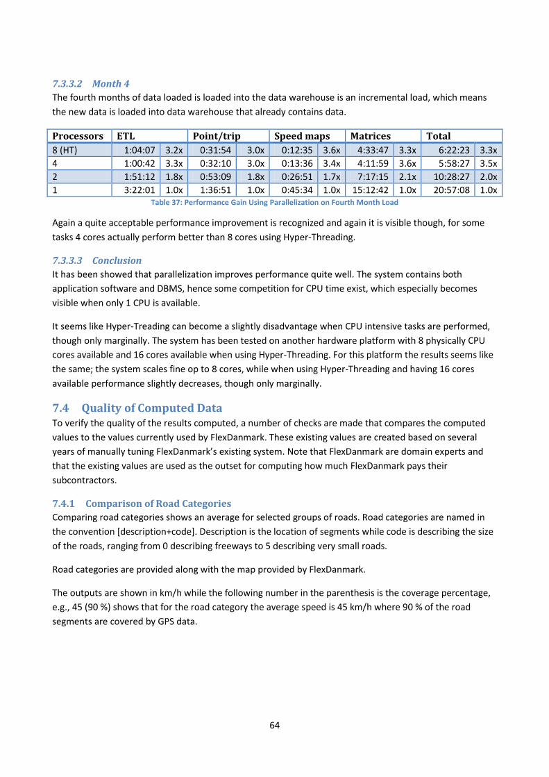
64

7.3.3.2 Month 4

The fourth months of data loaded is loaded into the data warehouse is an incremental load, which means

the new data is loaded into data warehouse that already contains data.

Processors ETL Point/trip Speed maps Matrices Total

8 (HT) 1:04:07 3.2x 0:31:54 3.0x 0:12:35 3.6x 4:33:47 3.3x 6:22:23 3.3x

4 1:00:42 3.3x 0:32:10 3.0x 0:13:36 3.4x 4:11:59 3.6x 5:58:27 3.5x

2 1:51:12 1.8x 0:53:09 1.8x 0:26:51 1.7x 7:17:15 2.1x 10:28:27 2.0x

1 3:22:01 1.0x 1:36:51 1.0x 0:45:34 1.0x 15:12:42 1.0x 20:57:08 1.0x Table 37: Performance Gain Using Parallelization on Fourth Month Load

Again a quite acceptable performance improvement is recognized and again it is visible though, for some

tasks 4 cores actually perform better than 8 cores using Hyper-Threading.

7.3.3.3 Conclusion

It has been showed that parallelization improves performance quite well. The system contains both

application software and DBMS, hence some competition for CPU time exist, which especially becomes

visible when only 1 CPU is available.

It seems like Hyper-Treading can become a slightly disadvantage when CPU intensive tasks are performed,

though only marginally. The system has been tested on another hardware platform with 8 physically CPU

cores available and 16 cores available when using Hyper-Threading. For this platform the results seems like

the same; the system scales fine op to 8 cores, while when using Hyper-Threading and having 16 cores

available performance slightly decreases, though only marginally.

7.4 Quality of Computed Data To verify the quality of the results computed, a number of checks are made that compares the computed

values to the values currently used by FlexDanmark. These existing values are created based on several

years of manually tuning FlexDanmark’s existing system. Note that FlexDanmark are domain experts and

that the existing values are used as the outset for computing how much FlexDanmark pays their

subcontractors.

7.4.1 Comparison of Road Categories

Comparing road categories shows an average for selected groups of roads. Road categories are named in

the convention [description+code]. Description is the location of segments while code is describing the size

of the roads, ranging from 0 describing freeways to 5 describing very small roads.

Road categories are provided along with the map provided by FlexDanmark.

The outputs are shown in km/h while the following number in the parenthesis is the coverage percentage,

e.g., 45 (90 %) shows that for the road category the average speed is 45 km/h where 90 % of the road

segments are covered by GPS data.

65

Road Category

Non-Peak Peak

Point Trip FlexDanmark Point Trip FlexDanmark

AA0 101.5 (97 %) 111.8 (69 %) 93 97.8 (97 %) 107.4 (62 %) 93

AA2 67.2 (95 %) 64.9 (62 %) 67 64.2 (94 %) 63.5 (57 %) 67

AA3 64.7 (93 %) 67.4 (52 %) 60 62.5 (93 %) 66.4 (46 %) 60

AA4 55.0 (92 %) 58.4 (25 %) 50 54.6 (92 %) 57.4 (20 %) 50

AA5 38.2 (75 %) 46.6 (0.4 %) 30 41.9 (64 %) 48.9 (2.7 %) 30 Table 38: Average Speeds and Coverage for Region Outside Aarhus City

The AA road categories are the Aarhus regions outside the city itself. The results for these roads are shown

in Table 38. The coverage is quite good, especially for point data. Trip data has a lower coverage, which

might indicate trip data is less accurate.

For both non-peak and peak period, the computed speeds are always faster than the FlexDanmark

predicted values, except for AA2. This is quite interesting and might indicate that the FlexDanmark

predictions are too conservative. Points and trips results are generally different, where trips always are

faster than points, except for AA2. As expected the speed is generally lower during peak hours compared to

non-peak hours. It is however interesting to observe, that for the smallest road the speeds actually

increases, during peak hours. It is properly due to insufficient GPS data sizes that this happens. Note that

the coverage for the smallest roads is considerable lower than for the other road categories.

Road Category

Non-Peak Peak


Aarhus2 51.9 (94 %) 51.1 (74 %) 40 46.0 (94 %) 48.3 (67 %) 40

Aarhus3 47.4 (97 %) 45.8 (57 %) 30 43.9 (97 %) 51.4 (46 %) 30

Aarhus4 40.3 (87 %) 41.0 (42 %) 20 38.8 (89 %) 42.1 (36 %) 20

Aarhus5 25.0 (80 %) 31.4 (4.7 %) 15 26.7 (72 %) 32.4 (4.1 %) 15 Table 39: Average Speeds and Coverage for Aarhus Suburbs

For the suburbs of Aarhus shown in Table 39 the trends are the same as in Table 38; the FlexDanmark

values are always lower than the computed speed and the coverage of the point data is much better than

the coverage of the trip data.

For point data, the peak periods are slower than the non-peak periods, except for the smallest roads. But

for trips data the peak speeds actually are faster than non-peak for three of the road categories.

Road Category

Non-Peak Peak


AAcity2 42.4 (98 %) 41.4 (77 %) 30 36.6 (97 %) 38.8 (74 %) 21

AAcity3 42.1 (92 %) 41.7 (66 %) 22 38.3 (92 %) 41.3 (62 %) 15

AAcity4 31.8 (87 %) 34.8 (44 %) 15 30.1 (87 %) 35.2 (39 %) 11

AAcity5 24.7 (86 %) 32.0 (11 %) 12 25.2 (81 %) 32.9 (5.1 %) 8 Table 40: Average Speeds and Coverage for Aarhus Urban Areas

Table 40 shows the speeds computed for the urban areas of Aarhus. Again the same picture shows, where

the computed speeds are much faster than the FlexDanmark’s speeds and the coverage is much better for

points than speeds.

66

Road Category

Non-Peak Peak


AAmetro2 32.7 (96 %) 39.6 (71 %) 30 29.7 (95 %) 39.3 (69 %) 21

AAmetro3 31.0 (98 %) 36.1 (75 %) 20 28.3 (98 %) 39.2 (63 %) 14

AAmetro4 28.3 (86 %) 31.2 (63 %) 14 27.5 (85 %) 31.6 (46 %) 10

AAmetro5 20.5 (92 %) 25.3 (29 %) 10 20.5 (90 %) 29.8 (16 %) 7 Table 41: Average Speeds and Coverage for Aarhus Metro Areas

For the inner areas of Aarhus city, the coverage is very good, especially for point data, as can be seen by

Table 41. The FlexDanmark speeds are much lower than the computed speeds again, and the trips speeds

are faster than the point speeds. For point data, the peak hours are a bit slower than non-peak, while for

trips peak hours actually is faster for category 2 through 4 than non-peak.

In general, the average speeds for different road categories closer to FlexDanmark’s estimated the closer

the roads categories are to the metro areas It only occurs once that the FlexDanmark speed is higher than

the computed speed, namely for road category AA2 using point data during peak. Trip speeds are generally

faster than point speeds.

Comparing peak and non-peak shows that non-peak speeds are faster than peak speeds with a few

exceptions. The reason for this can be that persons drive more aggressively during peak periods.

7.4.2 Central Roads in Around Aarhus

To compare roads with traffic in both directions, four road stretches have been compared. The results are

shown in Table 42.

Road name Category Non-Peak Peak


Ringgaden north AAmetro3 36.5 29.1 20 32.6 30.1 14

Ringgaden south AAmetro3 40.1 33.8 20 36.1 22.6 14

Ringvejen north AAcity2 40.2 31.4 30 35.2 31.1 21

Ringvejen south AAcity2 44.5 39.1 30 40.0 45.1 21

Freeway E45 north

AA0 110.0 105.0 93 105.0 103.0 93

Freeway E45 south

AA0 106.0 104.0 93 101.0 103.0 93

Freeway 15 east AA0 108.0 201.0 93 107.0 197.0 93

Freeway 15 west AA0 105.0 122.0 93 106.0 111.0 93 Table 42: Comparing Non-Peak and Peak Speeds

Looking at Table 42, it is clear that speed differences exist regarding in which directions vehicles travels.

Looking at both Ringgaden and Ringvejen the traffic is moving faster when driving south compared to

driving north. This is general for both point and trip data and indicates different traffic flow in the two

directions. Point data results mostly in higher values than trip data, while both point and trip data is always

higher than the FlexDanmark data – sometimes up to twice as fast.

When looking at the freeway E45, it is visible that traveling south is always slower than traveling north,

though the differences in speeds are small.

67

Freeway 15 east has some extraordinary high speeds in the east direction for trips. These speeds must be

discarded as a result of faulty computed trip data, incorrect GPS data, and only a low amount of trip data

available for the segment. However, the same pattern appears where there is a small difference in the

speed depending on the direction in which the vehicle is traveling.

Road name Category Morning Peak Afternoon Peak


Ringgaden north AAmetro3 32.3 32.3 14 33.0 36.9 14

Ringgaden south AAmetro3 37.0 36.5 14 35.0 40.0 14

Ringvejen north AAcity2 36.6 39.9 21 37.6 41.4 21

Ringvejen south AAcity2 40.8 48.4 21 39.1 42.2 21

Freeway E45 north

AA0 104.0 99.0 93 108.0 110.0 93

Freeway E45 south

AA0 101.0 105.0 93 101.0 101.0 93

Freeway 15 east AA0 107.0 202.0 93 107.0 174.0 93

Freeway 15 west AA0 108.0 113.0 93 104.0 110.0 93 Table 43: Comparing Morning Peak and Afternoon Peak

To investigate peak periods in more details, the peak speeds have been calculated for both morning and

afternoon peak and is showed in Table 43. Again the table contains some extraordinary high speeds for

freeway 15 east. Looking at Ringgaden and Ringvejen again it can be seen that in the direction north the

speed is higher during afternoon peak, while in the direction south the speed is higher during morning

peak. This indicates that more traffic flows north than south in the morning, while more traffic flows south

in the afternoon than in the morning. Point and trip data quite agree on the speeds in both directions.

Looking at the freeway E45 it can be seen that driving north the speed is higher in the afternoon than in the

morning, while driving south the speed is faster in the morning than in the afternoon. Looking at freeway

15 at least it can be seen that driving west is fastest in the morning, while the unusual high results for trips

does make it hard to conclude anything on driving east.

7.4.3 Comparison of Shortest Path between POIs

Drive-time matrices are a part of the output of the calculations. Some example pairs of from/to POIs have

been chosen to reflect both long and short distance transportations. For each pair of from/to POI, an

equivalent reversed from/to is being shown, to show whether differences exists in the two directions.

68

From To Non-Peak Peak FlexDanmark

Point Trip Point Trip

FRE208 ÅRH800 1:51:56 1:59:14 1:53:52 2:00:58 2:19:48

ÅRH800 FRE208 1:51:59 1:55:42 1:55:18 2:04:49 2:19:30

ÅRH780 ESB303 1:36:01 1:38:17 1:38:46 1:44:22 1:57:02

ESB303 ÅRH780 1:35:47 1:32:27 1:37:57 1:39:34 1:57:11

ÅRH800 THI752 1:51:24 2:07:21 1:51:20 2:16:15 2:26:41

THI752 ÅRH800 1:50:49 2:09:57 1:50:20 2:16:06 2:27:19

ÅRH780 ÅRH800 0:09:11 0:10:53 0:09:53 0:11:00 0:15:57

ÅRH800 ÅRH780 0:09:18 0:10:15 0:11:43 0:10:47 0:15:56

ÅRH780 ÅRH861 0:12:19 0:13:34 0:11:43 0:13:09 0:13:47

ÅRH861 ÅRH780 0:12:23 0:13:34 0:11:47 0:13:09 0:13:21

ÅRH800 ÅRH861 0:06:08 0:07:53 0:05:03 0:07:50 0:08:23

ÅRH861 ÅRH800 0:06:08 0:07:53 0:05:03 0:07:50 0:08:23 Table 44: Output of Drive-Time Matrices

Parts of the output data from the four drive-time matrices, for non-peak point, non-peak trip, peak point,

and peak trip, can be seen in Table 44. Overall, the point-based approach results in faster travel-times than

trip-based and trip based is always faster than FlexDanmark data. Also note that not of the compute travel

times are outrageous compared to the estimated values used by FlexDanmark.

The duration for a trip from POI to another and the duration for driving back again are very similar for all

the trips. This is probably caused by many of the segments being bidirectional, which means passing the

segment in each direction takes the same time.

7.4.4 Conclusion

From the experiments performed, it is shown that the system scales well for large data sizes. Even when

loading large quantities of data, the most time consuming part is computing drive-time matrices, which is

almost independent on the data size. Incremental load adds a small performance overhead to the system,

while it still is possible to load large data batches overnight. The system is optimized for parallel computing

and it is shown that the performance of most tasks scales linear with the number of processor cores

available.

When looking at the outputs it is clear that the computed speeds and drive times in general are faster than

the existing manually computed value. However, there is in general a good correlation between the results

and the results generally look reasonable. There are problems caused by incorrect data values. This results

in unrealistic values, e.g., the drive time becomes too high or too low.

8 Conclusion and Future Work This paper has in detailed documented the design and implementation of a complete software stack for

computing travel-time in road networks based on the GPS data. The software stack can be completely

based on open-source software. Each component in the software architecture has been described in

details. Overall the open-source software components are robust and perform very well. However, it has

been necessary to make customizations of the highly specialized and complicated component for map-

matching and trip generation.

69

A data warehouse for storing and querying the GPS data has been design and documented in details. The

ETL process for cleansing the GPS has been described with a focus on the overall data flow.

The software stack and data warehouse has been complete implemented and in use since March 2011. The

system has been tested on large scale real-world data sets. A detailed performance study has shown that

large data sets can be handled on a high-end desktop PC. In particular, the performance study has shown

that the use of parallel processes can significantly speed up the handling of the GPS data.

The output of the system is a number of travel-time matrixes for Denmark. Two approach has been

examined a point-based approach and a more data-intensive trip-based approach. Overall, the trip-based

approach reports faster travel-times than the point-based approach. Both approaches have been compared

to existing manually estimated travel-times. Overall the estimated travel-times are considerable longer.

This was expected since stop-times are included in the estimated values.

There are a number of directions for future research a particular problem identified is a more detailed

study why approximately 20% of the GPS data cannot be map-matched. In addition, a more detailed study

of why the trip-based approach is faster is also of great interest. An external map-matching/trip generation

component has been used. This component generally performs very well; however, it is used as a black-

box. It would be useful to study in more details if a larger portion of the GPS data can be used for trips than

with the current implementation.

9 Acknowledgement The work has been supported by Daisy Innovation, Cassiopeia Innovation, and the REDUCTION project

(www.reduction-project.eu). Thanks to Nick Christiansen and Niels T. Larsen from FlexDanmark for many

comments and suggestions on the platform.

10 Bibliography 1. Travel time studies with global positioning and geographic information systems: an integrated

methodology. Quiroga, Cesar Q. and Bullock, Darcy. 1-2, 1998, Transportation Research Part C: Emerging

Technologies, Vol. 6.

2. Comparison of Trip Determination Methods in Household Travel Surveys Enhanced by a Global Positioning

System. Forrest, Timothy L. and Pearson, David F. 2005, Transportation Research Record: Journal of the

Transportation Research Board.

3. Nusca, Andrew. Stockholm uses real-time GPS data to manage traffic congestion. SmartPlanet.com.

[Online] CBS Interactive Inc., April 16, 2010. [Cited: April 1, 2011.]

http://www.smartplanet.com/business/blog/smart-takes/stockholm-uses-real-time-gps-data-to-manage-

traffic-congestion/6098/.

4. IBM. IBM Helps City of Stockholm Predict Better Commuting Options. Press releases. [Online] IBM, April

16, 2010. [Cited: April 1, 2011.] http://www-03.ibm.com/press/us/en/pressrelease/29903.wss.

http://www.reduction-project.eu/

70

5. Dave Barth, Product Manager for Google Maps. The bright side of sitting in traffic: Crowdsourcing road

congestion data. The Official Google Blog. [Online] Google, August 25, 2009. [Cited: April 1, 2011.]

http://googleblog.blogspot.com/2009/08/bright-side-of-sitting-in-traffic.html.

6. Roy Williams, Software Engineer, Google Maps Team. You've got better things to do than wait in traffic.

The Official Google Blog. [Online] Google, March 7, 2011. [Cited: April 1, 2011.]

http://googleblog.blogspot.com/2011/03/youve-got-better-things-to-do-than-wait.html.

7. Chitu, Alex. Google Maps Predicts Traffic Conditions. Unofficial news and tips about Google. [Online]

Google Operating System Blog, April 17, 2008. [Cited: April 1, 2011.]

http://googlesystem.blogspot.com/2008/04/google-maps-predicts-traffic-conditions.html.

8. Murphy, David. Google Maps Dumps Driving Times With Traffic Estimates. PCMag.com. [Online] July 16,

2011. [Cited: May 30, 2012.] http://www.pcmag.com/article2/0,2817,2388607,00.asp.

9. TomTom. HD Traffic. [Online] TomTom. [Cited: April 1, 2011.]

http://www.tomtom.com/services/service.php?id=2.

10. —. Live Traffic. [Online] TomTom. [Cited: April 1, 2011.] http://www.tomtom.com/livetraffic.

11. Dynamic Travel Time Maps - Enabling Efficient Navigation. Pfoser, Dieter, Tryfona, Nectaria and

Voisard, Agnes. Vienna : Scientific and Statistical Database Management, July 24, 2006, pp. 369-378. 1551-

6393.

12. Using GPS to Measure Traffic System Performance. D'Este, Glen M., Zito, Rocco and Taylor, Michael A.

P. 4, s.l. : Computer-Aided Civil and Infrastructure Engineering, July 1999, Vol. 14, pp. 255-265.

13. Dynamic Vehicle Routing Based on Online Traffic Information. Fleischmann, Bernhard, Gnutzmann,

Stefan and Sandvoß, Elke. 4, s.l. : TRANSPORTATION SCIENCE, 2004, Vol. 38, pp. 420-433.

14. A TRAFFIC INFORMATION SYSTEM BY MEANS OF REAL-TIME FLOATING-CAR DAT. Schäfer, Ralf-Peter,

Thiessenhusen, Kai-Uwe and Wagne, Peter. s.l. : ITS World Congress, 2002, Vol. m, pp. 1-8.

15. Mazaré, Pierre-Emmanuel, et al., et al. Trade-offs between inductive loops and GPS probe vehicles for

travel time estimation: A mobile Century case study. 2008.

16. Pereira, Francisco, Costa, Hugo and Pereira, Nuno. An off-line map-matching algorithm for incomplete

map databases. European Transport Research Review. 1, 2009, 3, pp. 107-124.

17. Office of GEOINT Sciences . NGA: (U) World Geodetic System 1984 (UNCLASSIFIED):. [Online] March

2010. http://earth-info.nga.mil/GandG/wgs84/index.html.

18. OpenStreetMap - The Free Wiki World Map. [Online] [Cited: May 28, 2012.]

http://www.openstreetmap.org.

19. Open Geospatial Consortium. OGC Reference Model. 2011. OGC 08-062r7.

71

20. —. OpenGIS® Implementation Standard for Geographic information - Simple feature access - Part 1:

Common architecture. 2011. OGC 06-103r4.

21. Refractions Research, etc. PostGIS 2.0.0 Manual. 2012. SVN Revision (9605).

22. Kimball, Ralph and Ross, Margy. The Data Warehouse Toolkit: The Complete Guide to Dimensional

Modeling (Second Edition). s.l. : Wiley, 2002. 978-0471200246.

23. The PostgreSQL Global Development Group. PostgreSQL. [Online] [Cited: May 25, 2012.]

http://www.postgresql.org/.

24. Refractions Research. PostGIS. [Online] [Cited: May 23, 2012.] http://postgis.refractions.net/.

25. Python Software Foundation. Python Programming Language - Official Website. [Online] [Cited: May

25, 2012.] http://www.python.org/.

26. debian. debian. Debian -- The Universal Operating System. [Online] [Cited: April 6, 2011.]

http://www.debian.org/.

27. National Marine Electronics Association. NMEA 0183 Standard. NMEA. [Online] [Cited: February 10,

2011.] http://www.nmea.org/content/nmea_standards/nmea_083_v_400.asp.

28. DePriest, Dale. NMEA data. [Online] [Cited: February 4, 2011.]

http://www.gpsinformation.org/dale/nmea.htm.

29. Varrazzo, Daniele. PostgreSQL + Python | Psycopg. [Online] [Cited: May 25, 2012.]

http://initd.org/psycopg/.

30. Thomsen, Christian. ETL programming in Python. pygrametl. [Online] [Cited: February 10, 2011.]

http://www.pygrametl.org/.

31. NetworkX Developers. NetworkX v1.4 documentation. NetworkX . [Online] [Cited: February 10, 2011.]

http://networkx.lanl.gov/.

32. —. networkx.algorithms.shortest_paths.weighted.single_source_dijkstra. NetworkX. [Online] [Cited:

February 26, 2011.]

http://http://networkx.lanl.gov/reference/generated/networkx.algorithms.shortest_paths.weighted.single

_source_dijkstra.html.

33. —. networkx.algorithms.shortest_paths.weighted.single_source_dijkstra_path_length. NetworkX.

[Online] [Cited: February 26, 2011.]

http://networkx.lanl.gov/reference/generated/networkx.algorithms.shortest_paths.weighted.single_sourc

e_dijkstra_path_length.html.

34. Python. multiprocessing — Process-based parallelism: Managers. Python v3.2.3 documentation.

[Online] Python Software Foundation. [Cited: May 31, 2012.]

http://docs.python.org/py3k/library/multiprocessing.html#managers.

72

35. The PostgreSQL Global Development Group. 5.9. Partitioning. PostgreSQL 9.1.3 Documentation.

[Online] [Cited: May 25, 2012.] http://www.postgresql.org/docs/9.1/static/ddl-partitioning.html.

36. —. 45.48. pg_type. PostgreSQL 9.1.3 Documentation. [Online] [Cited: May 25, 2012.]

http://www.postgresql.org/docs/9.1/static/catalog-pg-type.html.

37. —. CLUSTER. PostgresSQL 9.1.4 Documentation. [Online] [Cited: June 26, 2012.]

http://www.postgresql.org/docs/9.1/static/sql-cluster.html.

38. Intel Corporation. Intel® Hyper-Threading Technology (Intel® HT Technology). [Online] [Cited: March

24, 2011.] http://www.intel.com/info/hyperthreading/.

39. Dijkstra, Edsgar Wybe. A note on two problems in connexion with graphs. Numerische Mathematik. 1,

1959, Vol. 1, pp. 269-271.

40. Psycopg. Server side cursors. Psycopg v2.3.1 documentation. [Online] [Cited: February 4, 2011.]

http://initd.org/psycopg/docs/usage.html#server-side-cursors.

41. —. Thread and process safety. Psycopg v2.3.1 documentation. [Online] [Cited: February 5, 2011.]

http://initd.org/psycopg/docs/usage.html#thread-and-process-safety.

42. Nakamura, Karen. Converting Latitude/Longitude to Universal Transverse Mercator (UTM). GPSy.

[Online] [Cited: February 10, 2011.] http://www.gpsy.com/gpsinfo/geotoutm/.

43. Gillies, Sean, Bierbaum, Aron and Lautaportti, Kai. Shapely. GIS-Python Lab. [Online] [Cited: February

10, 2011.] http://trac.gispython.org/lab/wiki/Shapely.

44. Gillies, Sean. Rtree: spatial index for Python GIS. GIS-Python Lab. [Online] [Cited: February 10, 2011.]

http://trac.gispython.org/lab/wiki/Rtree.

45. Hadjieleftheriou, Marios. Spatial Index. [Online] [Cited: February 10, 2011.]

http://trac.gispython.org/spatialindex/wiki.

46. Guttman, Antonin. R-trees: a dynamic index structure for spatial searching. SIGMOD Rec. June 1984,

Vol. 14, 2, pp. 47-57.

47. Nelson, Russ. LatLonUTMconversion. Russ Nelsons : gis. [Online] [Cited: February 11, 2011.]

http://blog.russnelson.com/gis/index.html.

48. Wikipedia. MSConfig. Wikipedia, the free encyclopedia. [Online] [Cited: March 24, 2011.]

http://en.wikipedia.org/wiki/MSConfig.

49. IBM. Driving change in Stockholm. How it works. [Online] IBM, April 3, 2007. [Cited: April 1, 2011.]

http://www.ibm.com/podcasts/howitworks/040207/images/HIW_04022007.pdf.

50. Lawhead, Joel. pyshp - Python Shapefile Library. [Online] [Cited: May 25, 2012.]

http://code.google.com/p/pyshp/.

73

51. Bishop, Stuart. pytz - World Timezone Definitions for Python. [Online] [Cited: May 25, 2012.]

http://pytz.sourceforge.net/.

52. Environmental Systems Research Institute, Inc. ESRI Shapefile Technical Description. [Online] 1998.

http://www.esri.com/library/whitepapers/pdfs/shapefile.pdf.

74

11 Appendix: External Limitation and Assumptions The system using GPS data and a digital map makes implicit assumption that can have an effect on the

accuracy of the computed drive times. The limitations are the following.

Trips from all drivers are aggregated into a single result. This means that if there is an over

representation of young aggressive drivers the drive times may be lower than what an average

driver will experience in real-life.

The speed for a single GPS position only records the speed of the vehicle at a very specific instance.

As an example, if there are 15 seconds between consecutive GPS points from a single vehicle the

vehicle may have driver 50 km/h in the first 13 seconds. However, in the last two seconds the

vehicle accelerates to 70 km/h. The GPS position will only report the latter speed.

The GPS points from a single driver, on a single trip are aggregated at the segment level. This leads

to an inaccuracy in the compute drive time, similar to the problem described above with a vehicle

accelerating. However, the segment is the finest granularity available in the digital map and is

therefore an external limitation.

The driver may behave irrational when driving, e.g., driving slower than then allowed on a Sunday

afternoon trip. It is hard, if not impossible, to detect such irrational driving. However, it is assumed

that the number of these trips is very small compared to the number of rational trips.

75

12 Appendix: Changes to M-GEMMA

12.1 Custom Path to Map The standard M-GEMMA loads its map from the path “data/map.txt”, but in order to load the map from a

different path, the main file is altered slightly.

In the file Main.h the description of the function to load the map has been changed from:

void loadMap();

to:

void loadMap(const std::string& folder);

In the file Main.cpp the following line has been added after line 14, to generate a variable containing the

path to the map:

std::string mapFolder;

In Main.cpp, the following has been changed, in order to make help description up to date, from:

<< " -M -> generate Map Matching .kml files" << std::endl

<< " -h -> help" << std::endl

to:

<< " -M -> generate Map Matching .kml files" << std::endl

<< " -map [folder] -> path to map file (the default path is data/map.txt)" <<

std::endl

<< " -h -> help" << std::endl

To load argument the argument given M-GEMMA, the following is changed in Main.cpp from:

else if (strcmp(argv[i], "-M") == 0)

marchalKML = geneticKML = true;

}

to:

else if (strcmp(argv[i], "-M") == 0)

marchalKML = geneticKML = true;

else if (strcmp(argv[i], "-map") == 0)

mapFolder = std::string(argv[++i]);

}

In Main.cpp the function loading the map, has be changed in order to take the path the map as argument

from:

loadMap();

to:

loadMap(mapFolder);

At last, the map loading function is changed to load the map from the path in Main.cpp from:

76

void loadMap()

{

std::stringstream path;

path << "data" << FILE_SEPARATOR << "map.txt";

std::cout << "Trying to load map: " << path.str() << std::endl;

m = mapRepresentation::Map(path.str());

}

to:

void loadMap(const std::string& path)

{

std::cout << "Trying to load map: " << path << std::endl;

m = mapRepresentation::Map(path);

}

12.1.1.1 Windows Compilation

For compiling on Windows, line 144 and 148 of the file quadtree.cpp must be changed from

return pair<QuadLeafNode *, QuadInnerNode *>(NULL, NULL);

to

return pair<QuadLeafNode *, QuadInnerNode *>();

due to a conversion error when compiling.

Compilation of M-GEMMA on Windows is easily done by using Microsoft Visual Studios x64 command

prompt, using the compiler and linker cl.exe. The compilation is done with the following command:

cl.exe -o mgemma.exe /O2 src\*.cpp /D "_UNICODE" /D "UNICODE" /EHsc

The output of the compilations is the file mgemma.exe. The /O2 option tells to optimize for speed and

the two /D options tells to compile for Unicode. The /EHsc option tells the compiler to specify

synchronous exception handling and assume extern C++ functions to never through exceptions.

12.2 Linux Compilation When compiling under Linux (Debian) two header files needs to be altered, in order to compile correctly.

In Main.h after line 15, the following include is added:

#include <cstring>

In the file matching_genetic_util.h, after line 8 the following three includes are added:

#include <climits>

#include <cstring>

#include <cstdlib>

The cstring library defines functions to manipulate strings and arrays, while the library climits

defines system specific constants. The cstdlib library defines several functions for memory

management, random generation, converting, sorting, searching, communication, and arithmetic. These

headers are probably a part of the general compiler headers in Windows, while on Linux they must be

specifically defined.

77

To compile M-GEMMA on Linux, the g++ compiler can be used like:

g++ src/*.cpp -O2 -o mgemma

The –O2 option tells the compiler to optimize for speed. The –o option tells the compiler to link all the files

together in one executable file called mgemma.

12.3 Memory The memory footprint of M-GEMMA is important to notice. About 5GB of memory is needed when using

the entire map of Denmark, thus a 64 bit version is needed. The memory usage is solely dependent on the

size of the map.

It is worth to notice, that exception handling in M-GEMMA is very limited. As an example, M-GEMMA

terminates without any notice if the input format is wrong. However, a detailed study of the output of M-

GEMMA shows that the map-matching is good.

78

13 Appendix: NetworkX Improved Algorithm A NetworkX function is used to compute the shortest path from a single source to all other sources in a

graph, (32). The original algorithm is shown below.

def single_source_dijkstra(G, source, target=None, cutoff=None, weight='weight'):

"""Compute shortest paths and lengths in a weighted graph G.

Uses Dijkstra's algorithm for shortest paths.

Parameters

----------

G : NetworkX graph

source : node label

Starting node for path

target : node label, optional

Ending node for path

cutoff : integer or float, optional

Depth to stop the search. Only paths of length <= cutoff are returned.

Returns

-------

distance,path : dictionaries

Returns a tuple of two dictionaries keyed by node.

The first dictionary stores distance from the source.

The second stores the path from the source to that node.

Examples

--------

>>> G=nx.path_graph(5)

>>> length,path=nx.single_source_dijkstra(G,0)

>>> print(length[4])

4

>>> print(length)

{0: 0, 1: 1, 2: 2, 3: 3, 4: 4}

>>> path[4]

[0, 1, 2, 3, 4]

Notes

---------

Distances are calculated as sums of weighted edges traversed.

Edges must hold numerical values for Graph and DiGraphs.

Based on the Python cookbook recipe (119466) at

http://aspn.activestate.com/ASPN/Cookbook/Python/Recipe/119466

This algorithm is not guaranteed to work if edge weights

are negative or are floating point numbers

(overflows and roundoff errors can cause problems).

See Also

--------

single_source_dijkstra_path()

single_source_dijkstra_path_length()

"""

if source == target: return (0, [source])

dist = {} # dictionary of final distances

paths = {source:[source]} # dictionary of paths

seen = {source:0}

fringe = [] # use heapq with (distance,label) tuples

heapq.heappush(fringe, (0, source))

while fringe:

(d, v) = heapq.heappop(fringe)

if v in dist: continue # already searched this node.

dist[v] = d

if v == target: break

#for ignore,w,edgedata in G.edges_iter(v,data=True):

79

#is about 30% slower than the following

if G.is_multigraph():

edata = []

for w, keydata in list(G[v].items()):

minweight = min((dd.get(weight, 1)

for k, dd in keydata.items()))

edata.append((w, {weight:minweight}))

else:

edata = iter(G[v].items())

for w, edgedata in edata:

vw_dist = dist[v] + edgedata.get(weight, 1)

if cutoff is not None:

if vw_dist > cutoff:

continue

if w in dist:

if vw_dist < dist[w]:

raise ValueError("Contradictory paths found: negative weights?")

elif w not in seen or vw_dist < seen[w]:

seen[w] = vw_dist

heapq.heappush(fringe, (vw_dist, w))

paths[w] = paths[v] + [w]

return (dist, paths)

The output of the algorithm is the distance to all other sources along with the paths to these. There are

some features that make the algorithm inefficient in the current setting.

1. It is unnecessary to return the paths to all the sources. NetworkX actually has a function only

returning the distance, (33), but this calls the function shown above and only returns the distance

from this.

2. The algorithm runs out of memory when the map is of a certain size. Particular a problem, when

running on a 32 bit platform.

3. This project requires both the shortest distance between the points of the maps as an output along

with the actually length of the path. This is not possible using the above algorithm.

To overcome these issues, a derived algorithm has been developed from the above. The algorithm follows,

with stripped out initial description:

def single_source_dijkstra_new(G, source, weight='weight', weight2=None):

"""Method fetched from networkx.single_source_dijkstra.

Altered and improved for better memory usage and ability of secondary

weight.

:param G: Graph for performing shortest path on.

:param source: Source node, to compute all paths from.

:param weight: Default weight to minimize shortest path from.

:param weight2: Secondary weight to calculate beside weight.

:return: Tuple of two dictionaries (weight1, weight2). Both

dictionaries have nodeids as keys and output values as values.

weight1 contains the weight being minimized for, and weight2 is the

optionally computed weight.

"""

import heapq

dist = {} # dictionary of final distances

sec_val = {}

seen = {source: 0}

fringe = [] # use heapq with (distance,label) tuples

heapq.heappush(fringe, (0, 0, source))

minweight2 = 0

while fringe:

(d, d2, v) = heapq.heappop(fringe)

if v in dist:

continue # already searched this node.

dist[v] = d

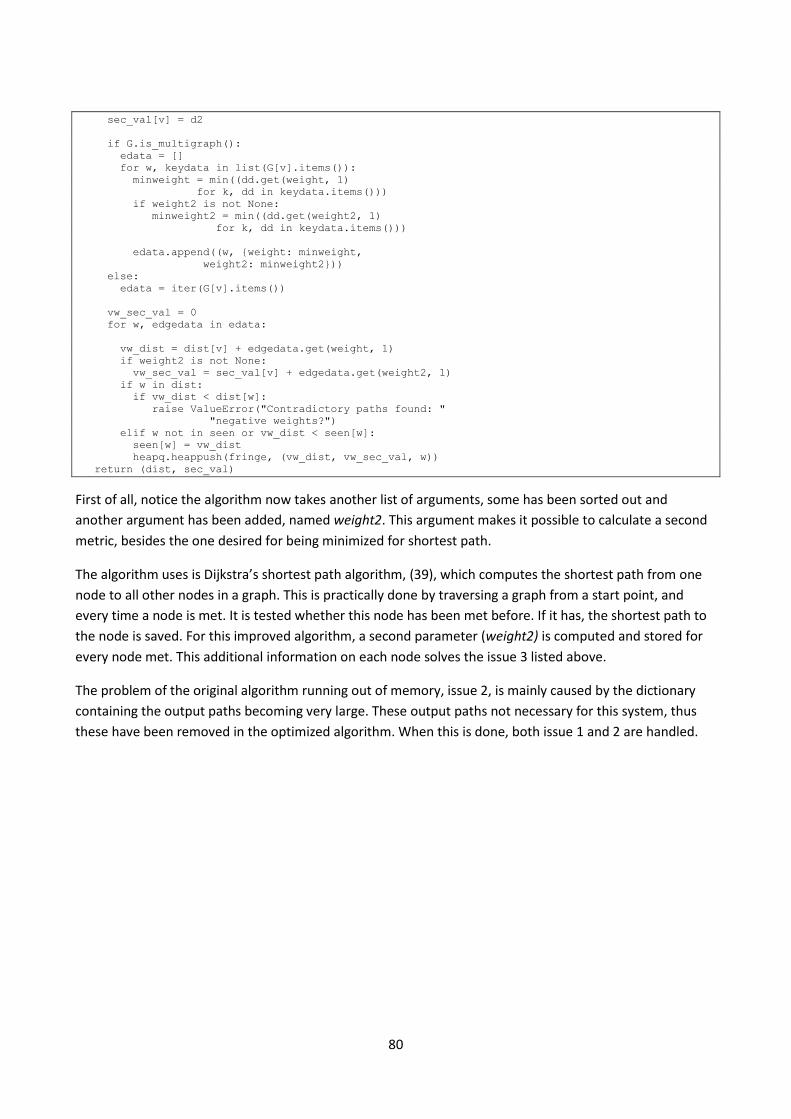
80

sec_val[v] = d2

if G.is_multigraph():

edata = []

for w, keydata in list(G[v].items()):

minweight = min((dd.get(weight, 1)


if weight2 is not None:

minweight2 = min((dd.get(weight2, 1)


edata.append((w, {weight: minweight,

weight2: minweight2}))

else:

edata = iter(G[v].items())

vw_sec_val = 0

for w, edgedata in edata:

vw_dist = dist[v] + edgedata.get(weight, 1)

if weight2 is not None:

vw_sec_val = sec_val[v] + edgedata.get(weight2, 1)

if w in dist:

if vw_dist < dist[w]:

raise ValueError("Contradictory paths found: "

"negative weights?")

elif w not in seen or vw_dist < seen[w]:

seen[w] = vw_dist

heapq.heappush(fringe, (vw_dist, vw_sec_val, w))

return (dist, sec_val)

First of all, notice the algorithm now takes another list of arguments, some has been sorted out and

another argument has been added, named weight2. This argument makes it possible to calculate a second

metric, besides the one desired for being minimized for shortest path.

The algorithm uses is Dijkstra’s shortest path algorithm, (39), which computes the shortest path from one

node to all other nodes in a graph. This is practically done by traversing a graph from a start point, and

every time a node is met. It is tested whether this node has been met before. If it has, the shortest path to

the node is saved. For this improved algorithm, a second parameter (weight2) is computed and stored for

every node met. This additional information on each node solves the issue 3 listed above.

The problem of the original algorithm running out of memory, issue 2, is mainly caused by the dictionary

containing the output paths becoming very large. These output paths not necessary for this system, thus

these have been removed in the optimized algorithm. When this is done, both issue 1 and 2 are handled.

an open-source its platform - aalborg universitetdbtr.cs.aau.dk/dbpublications/dbtr-32.pdf · an...

Documents