an optimal control approach to mission planning problems ... · pdf filean optimal control...

Calhoun: The NPS Institutional Archive

Theses and Dissertations Thesis and Dissertation Collection

2014-12

An optimal control approach to mission

planning problems: a proof of concept

Greenslade, Joseph Micheal

Monterey, California: Naval Postgraduate School

http://hdl.handle.net/10945/49611

NAVAL POSTGRADUATE

SCHOOL MONTEREY, CALIFORNIA

THESIS

Approved for public release; distribution is unlimited

AN OPTIMAL CONTROL APPROACH TO MISSION PLANNING PROBLEMS: A PROOF OF CONCEPT

by

Joseph M. Greenslade

December 2014

Thesis Co-Advisors: I. M. Ross M. Karpenko

THIS PAGE INTENTIONALLY LEFT BLANK

i

REPORT DOCUMENTATION PAGE Form Approved OMB No. 0704–0188 Public reporting burden for this collection of information is estimated to average 1 hour per response, including the time for reviewing instruction, searching existing data sources, gathering and maintaining the data needed, and completing and reviewing the collection of information. Send comments regarding this burden estimate or any other aspect of this collection of information, including suggestions for reducing this burden, to Washington headquarters Services, Directorate for Information Operations and Reports, 1215 Jefferson Davis Highway, Suite 1204, Arlington, VA 22202–4302, and to the Office of Management and Budget, Paperwork Reduction Project (0704–0188) Washington DC 20503.

1. AGENCY USE ONLY (Leave blank)

2. REPORT DATE December 2014

3. REPORT TYPE AND DATES COVERED Master’s Thesis

4. TITLE AND SUBTITLE AN OPTIMAL CONTROL APPROACH TO MISSION PLANNING PROBLEMS: A PROOF OF CONCEPT

5. FUNDING NUMBERS

6. AUTHOR(S) Joseph M. Greenslade

7. PERFORMING ORGANIZATION NAME(S) AND ADDRESS(ES) Naval Postgraduate School Monterey, CA 93943–5000

8. PERFORMING ORGANIZATION REPORT NUMBER

9. SPONSORING /MONITORING AGENCY NAME(S) AND ADDRESS(ES) N/A

10. SPONSORING/MONITORING AGENCY REPORT NUMBER

11. SUPPLEMENTARY NOTES The views expressed in this thesis are those of the author and do not reflect the official policy or position of the Department of Defense or the U.S. Government. IRB protocol number ____N/A____.

12a. DISTRIBUTION / AVAILABILITY STATEMENT Approved for public release; distribution is unlimited

12b. DISTRIBUTION CODE A

13. ABSTRACT (maximum 200 words)

This work introduces the use of optimal control methods for simultaneous target sequencing and dynamic trajectory planning of an autonomous vehicle. This is achieved by deriving a control solution that minimizes a cost to maximize target selection. In the case of varying target priorities, the method described here preferentially selects higher priority targets to maximize total benefit in the allowed time horizon. Traditional techniques employ heuristic techniques for target sequencing and then apply a separate trajectory planning process to check the feasibility of the sequence for the given vehicle dynamics. This work uses pseudospectral methods to deterministically solve the problem in a single step. The historic barrier to the application of optimal control solutions to the target sequencing problem has been the requirement for a problem formulation built from continuous constraints. Target points are, by their nature, discrete. The key breakthrough is to transform the discrete problem into a continuous representation by modeling targets as Gaussian distributions. The proposed approach is successfully applied to several benchmark problems. Thus, several variations of the so-called motorized travelling salesman problem, including ones in which it is impossible to acquire all the targets in the given time, are solved using the new approach. 14. SUBJECT TERMS Optimization, Optimal Control, Travelling Salesman Problem, Orienteering Problem, Mission Planning, Path Selection, Target Selection, Target Priorities, Pseudospectral Methods, DIDO

15. NUMBER OF PAGES

107

16. PRICE CODE

17. SECURITY CLASSIFICATION OF REPORT

Unclassified

18. SECURITY CLASSIFICATION OF THIS PAGE

Unclassified

19. SECURITY CLASSIFICATION OF ABSTRACT

Unclassified

20. LIMITATION OF ABSTRACT

UU NSN 7540–01–280–5500 Standard Form 298 (Rev. 2–89) Prescribed by ANSI Std. 239–18

ii


iii

Approved for public release; distribution is unlimited

AN OPTIMAL CONTROL APPROACH TO MISSION PLANNING PROBLEMS: A PROOF OF CONCEPT

Joseph M. Greenslade Lieutenant Commander, United States Navy

B.A., Texas A&M University, 1994 B.S., Texas A&M University, 1998

Submitted in partial fulfillment of the requirements for the degree of

MASTER OF SCIENCE IN ASTRONAUTICAL ENGINEERING

from the

NAVAL POSTGRADUATE SCHOOL December 2014

Author: Joseph Micheal Greenslade

Approved by: I. Michael Ross Thesis Co-Advisor

Mark Karpenko Thesis Co-Advisor

Garth Hobson Chair, Department of Mechanical and Aerospace Engineering

iv


v

ABSTRACT

This work introduces the use of optimal control methods for simultaneous target

sequencing and dynamic trajectory planning of an autonomous vehicle. This is achieved

by deriving a control solution that minimizes a cost to maximize target selection. In the

case of varying target priorities, the method described here preferentially selects higher

priority targets to maximize total benefit in the allowed time horizon. Traditional

techniques employ heuristic techniques for target sequencing and then apply a separate

trajectory planning process to check the feasibility of the sequence for the given vehicle

dynamics. This work uses pseudospectral methods to deterministically solve the problem

in a single step. The historic barrier to the application of optimal control solutions to the

target sequencing problem has been the requirement for a problem formulation built from

continuous constraints. Target points are, by their nature, discrete. The key breakthrough

is to transform the discrete problem into a continuous representation by modeling targets

as Gaussian distributions. The proposed approach is successfully applied to several

benchmark problems. Thus, several variations of the so-called motorized travelling

salesman problem, including ones in which it is impossible to acquire all the targets in the

given time, are solved using the new approach.

vi


vii

TABLE OF CONTENTS

I. INTRODUCTION........................................................................................................1 A. MOTIVATION ................................................................................................1 B. PREVIOUS WORK .........................................................................................3 C. THESIS OBJECTIVE .....................................................................................5 D. THESIS OUTLINE ..........................................................................................7

II. OPTIMAL CONTROL PROCESSES .......................................................................9 A. THE MATHEMATICAL THEORY OF OPTIMAL PROCESSES ........10 B. METHODOLOGY FOR SOLVING OPTIMAL CONTROL

PROBLEMS ...................................................................................................15 1. Shooting ..............................................................................................15 2. Collocation ..........................................................................................16 3. Pseudospectral Theory ......................................................................16

C. CODING AN OPTIMAL CONTROL PROBLEM IN DIDO ...................17

III. THE OBSTACLE AVOIDANCE PROBLEM .......................................................19 A. OBSTACLES AS A PATH FUNCTION .....................................................19 B. OBSTACLES AS A COST PENALTY FUNCTION .................................21

IV. THE MISSION PLANNING PROBLEM ...............................................................27 A. VEHICLE DYNAMICS ................................................................................27 B. TARGET DEFINITION ...............................................................................29 C. MISSION PLANNING METHOD: THE STICK AND THE

CARROT ........................................................................................................37

V. SPARSE TARGET FIELD .......................................................................................39 A. TARGETS WITH EQUAL PRIORITY ......................................................39

1. Setting Up the Problem .....................................................................40 2. Same Target Priority Mission Planning Problem ...........................45

B. TARGETS WITH VARYING PRIORITIES .............................................50 C. SUMMARY ....................................................................................................55

VI. MISSION PLANNING IN A TARGET RICH FIELD ..........................................57 A. TARGETS WITH EQUAL PRIORITY ......................................................57 B. PRIORITIZED TARGETS...........................................................................62

1. Seeding the Algorithm .......................................................................64 2. Solutions in a Prioritized Target Rich Field ....................................67

C. CONCLUSION ..............................................................................................69

VII. BENCHMARK PROBLEM: MOTORIZED TRAVELLING SALESMAN ......71 A. TWO METHODS FOR SOLVING THE MTSP WITH HYBRID

OPTIMAL CONTROL .................................................................................71 1. Methodology .......................................................................................71 2. Problem Definition .............................................................................72

a. System Dynamics.....................................................................72 b. City Locations ..........................................................................72

viii

3. Problem Solution ................................................................................73 B. SOLVING THE MTSP WITH THE PSEUDOSPECTRAL

OPTIMAL CONTROL MISSION PLANNING METHOD .....................74 C. CONCLUSION ..............................................................................................79

VIII. CONCLUSIONS ........................................................................................................81 A. RESEARCH CONCLUSIONS .....................................................................81 B. FUTURE WORK ...........................................................................................81

1. Target Revisit and Subtours .............................................................81 2. Elimination of Aggregate Peaks in Potential Field .........................82

a. Iterative Solution with Reduced σ on Successive Steps .........83 b. Dynamic σ Based on Vehicle Distance to Targets .................83

3. Time Windows ....................................................................................83 4. Application to More Complex Systems ............................................83

LIST OF REFERENCES ......................................................................................................85

INITIAL DISTRIBUTION LIST .........................................................................................89

ix

LIST OF FIGURES

Figure 1 ISR platforms: (a) WorldView1 (DigitalGlobe); (b) F/A-18F with SHARP (Shared Reconnaissance Pod) (USN); (c) XM1216 SUGV (Small Unmanned Ground Vehicle) (USA); (d) MQ-9 Reaper (USAF) .......................2

Figure 2 Possible paths vs. number of targets, from [6] ...................................................4 Figure 3 Unit p-norms for p =1, 2 and 100, after [12]. ..................................................12 Figure 4 Obstacle avoidance path. .................................................................................20 Figure 5 Propagated trajectories and optimal control solutions. ....................................21 Figure 6 Hamiltonian value of the obstacle avoidance problem. ...................................21 Figure 7 Obstacle avoidance path with penalty cost function. .......................................23 Figure 8 Propagated trajectories and optimal control solutions of obstacle

avoidance path with penalty cost function. ......................................................24 Figure 9 Hamiltonian value of obstacle avoidance path with penalty cost function. .....25 Figure 10 Example targets in a field. ...............................................................................29

Figure 11 Indicator function plot of target set L̂ . .......................................................30

Figure 12 Priority scaled indicator function plot of set ˆpL ..........................................31

Figure 13 Dirac-d function ...............................................................................................33

Figure 14 Sinc function. ...................................................................................................34 Figure 15 Normalized exponential (Gaussian) function ..................................................35 Figure 16 Two-dimensional normalized Gaussian function ............................................36 Figure 17 Exponential (Gaussian) approximation of the prioritized indicator

function. ...........................................................................................................37 Figure 18 Exponential (Gaussian) approximation of the prioritized indicator function

of the benefit (a) and penalty (b) for a single target. .......................................38 Figure 19 Benefit function for sparse target field. ...........................................................39 Figure 20 Potential field, both benefit (a) and penalty (b), as experienced by a

vehicle, (X) on the target located at (3,3) in the example target set. ................42 Figure 21 Potential field generated by benefit (a) and penalty (b) function for sparse

target field with equal priorities. ......................................................................45 Figure 22 Optimal path through sparse target field with equal priority targets. ..............46 Figure 23 Plot of Hamiltonian value ................................................................................47 Figure 24 Scaled states and costates of optimal path for sparse field with equal

priority targets. .................................................................................................47 Figure 25 Propagated trajectories and optimal control solutions. ....................................48 Figure 26 Single priority sparse target field: (a) minimum time; (b) 2 targets; (c) 3

targets; (d) 4 targets. ........................................................................................49 Figure 27 Potential field generated by benefit (a) and penalty (b) function for sparse

target field, different target priorities ...............................................................50 Figure 28 Optimal path through sparse target field with prioritized targets. ...................51 Figure 29 Scaled states and costates of optimal path .......................................................52 Figure 30 Plot of Hamiltonian value ................................................................................53 Figure 31 Switching function ...........................................................................................53

x

Figure 32 Propagated trajectories and optimal control solutions. ....................................54 Figure 33 Multiple priority sparse target field: (a) minimum time; (b) 2 targets; (c) 3

targets; (d) 4 targets. ........................................................................................55 Figure 34 Potential field generated by benefit (a) and penalty (b) function for target

rich field with equal priorities. .........................................................................58 Figure 35 Potential field generated by benefit (a) and penalty (b) function for sparse

target field with equal priorities. ......................................................................59 Figure 36 Optimal path in a target rich field with equal priority targets. .........................60 Figure 37 Paths through a target rich field with equal target priorities and

constrained time: (a) minimum time; (b) 30 TU; (c) 31 TU; (d) 35 TU. .........61 Figure 38 Potential field generated by benefit and penalty function for target rich

field with prioritized targets. ............................................................................62 Figure 39 Target values in rich field with priority targets. ..............................................63 Figure 40 Potential field generated by benefit and penalty function for target rich

field with prioritized targets with σ = 0.1. .......................................................64 Figure 41 Paths for varying time horizons using different seeds: (a) target set sorted

on X position; (b) target set sorted on Y position; (c) target set sorted by Euclidian distance from start point; (d) target set sorted by priority. ..............66

Figure 42 Paths in target rich field: prioritized targets (black); equal priority targets (red). .................................................................................................................67

Figure 43 Multiple priority target rich field: (a) minimum time; (b) 17 TU; (c) 25 TU; (d) 30 TU. .................................................................................................68

Figure 44 The five minimum time solution candidates obtained for the MTSP with three cities, from [8]. ........................................................................................73

Figure 45 Optimal paths for cities 1, 2, and 3, from [10]. ................................................74 Figure 46 Potential field generated by benefit (a) and penalty (b) for 10 city target

set. ....................................................................................................................77 Figure 47 Optimal solution to MTSP through cities 1, 2, and 3. .....................................77 Figure 48 Scaled states and costates of optimal solution to the MSTP. ...........................78 Figure 49 Plot of the Hamiltonian value of MTSP. .........................................................79 Figure 50 Comparison of path selected with single priority target sets and different

values for : sparse target, 21.34 TU (a) 0.1 ; (b) 0.5 ; target rich, 31 TU (c) 0.1 ; (d) 0.5 . ......................................................................82

xi

LIST OF TABLES

Table 1 Summary of results for mission planning in an equal priority sparse target field. .................................................................................................................50

Table 2 Summary of results for mission planning in a multiple priority sparse target field. .......................................................................................................55

Table 3 Different seeds for initializing the mission planning algorithm. .....................65 Table 4 Locations of cities for MTSP, after [8]. ...........................................................72 Table 5 Modified list of city locations, from [10]. ........................................................73

xii


xiii

LIST OF ACRONYMS AND ABBREVIATIONS

BGain benefit gain

BVP boundary value problem

GA genetic algorithm

HOC hybrid optimal control

ISR intelligence, surveillance, and reconnaissance

KKT Karush-Kuhn-Tucker

MP mission planning

MTSP motorized travelling salesman problem

NP non-deterministic polynomial-time

OA obstacle avoidance

OP orienteering problem

PGain penalty gain

PS pseudospectral

SHARP shared reconnaissance pod

SUGV small unmanned ground vehicle

TSP travelling salesman problem

TU time unit

UAV unmanned aerial vehicle

UGV unmanned ground vehicle

V&V validation and verification

xiv


xv

ACKNOWLEDGMENTS

First and foremost, I want to thank my wife. Valerie has given me all the support

I needed. And that is no small thing, since that support involved taking care of our

three daughters, Moira, Caitlin, and Bridget, when I was too busy to help out. I could

not have enjoyed the success I have in graduate school without her. And nothing in life

would be as good as it is without her and our girls. So, I am going to work very hard to

make up to all of them for the time I spent working on my research instead of with them.

Dr. Ross and Dr. Karpenko were outstanding teachers and mentors, guiding

my research and keeping me on track. I freely admit that the research was more fun

than the writing. And if it was not for my advisors, I probably never would have

stopped modifying my algorithm. I explored questions in areas I did not know

existed and learned a lot more over the last two years than I ever thought I would.

I would be remiss if I didn’t acknowledge my cohort mates. The Space Cave, and

the Guidance, Navigation and Control Lab were great environments for learning, as well

as discussions of almost any topic. I’m lucky to have gone to school with such a great

group of people.

xvi


1

I. INTRODUCTION

The intent of this research is to provide a proof of concept for the use of optimal

control methods to accomplish mission planning in a target field where the number of

targets that can be collected is much less than the total number of opportunities. Mission

planning includes: target selection, path planning and motion control problems of a

modeled vehicle. An example from practice is an imaging satellite where the mission

planner must decide which of the desired targets will be imaged in the available imaging

window. While this thesis does not deal with the complex dynamics of an imaging

satellite, the goal is to develop and validate a mission planning process that can be

adapted to just such a system.

The dynamics for the purpose of this thesis is the kinematics of a mobile robot.

Simple dynamics were used in order to simplify the problem so that attention could be

focused on the complexity of the mission planning problem that is common to all

vehicles, instead of on complex dynamics of a particular vehicle.

A. MOTIVATION

Mission planning for intelligence, surveillance, and reconnaissance (ISR) assets is

an exceedingly complex endeavor that can be broken down into three broad tasks. First,

targets of interest must be identified and prioritized. Priorities are assigned by targeteers,

intelligence analysts or, in the case of commercial ISR assets, the customer. The priorities

based on the relative importance of the targets in a target set. Target prioritization is a

field of study unto itself, and as such, is beyond the scope of this thesis [1]. Next, ISR

assets must be assigned. Lastly, mission plans for those assets must be developed and

executed. The intent of this research is to demonstrate how optimal control methods can

be used to accomplish path planning and motion control of ISR assets in a target rich

environment. In this context a target rich environment is one in which, due to time limits

or kinematic constraints, the ISR asset cannot visit all designated targets.

Current metrics for satellite photo reconnaissance focus on total imaged area, in

square kilometers or square miles, or number of images taken [2]. This research proposes

2

a mission planning process that maximizes a more appropriate quantitative measure: the

benefit value of the images taken (or targets visited) by a satellite, or any other ISR asset.

Figure 1 ISR platforms: (a) WorldView1 (DigitalGlobe); (b) F/A-18F with SHARP (Shared Reconnaissance Pod) (USN); (c) XM1216 SUGV

(Small Unmanned Ground Vehicle) (USA); (d) MQ-9 Reaper (USAF)

ISR assets can be satellites, unmanned aerial vehicles (UAVs), manned aircraft, or

surface vehicles. The mission planning algorithm developed here should therefore be

agnostic to the ISR platform employed. Ideally it is only the dynamics that will have to

be changed in the problem formulation to those of the platform being employed. This

aspect represents one significant benefit of the new approach.

3

B. PREVIOUS WORK

In mathematics, the mission planning problem as defined here, is an orienteering

problem (OP), which is related to the travelling salesman problem (TSP). The TSP has

been a subject of serious research for at least the last 80 years, but has existed as a

practical problem for hundreds of years [3]. The TSP seeks to find the best circuit

through a given set of cities beginning and finishing at the same city and visiting every

city no more than once. There is a cost associated with travelling between each of the

cities, usually distance or time of travel. The best circuit through the cities is the one that

minimizes the cost of the travel. The OP seeks to maximize the value of the route taken

by visiting either as many sites as it can, or by visiting sites with a higher relative value

than other sites in a given time horizon. Unlike the TSP, in the OP the first and last sites

are not required to be the same [4]. Moreover in the OP, it may not be necessary to visit

all the cities.

The mission planning problem is an OP with target specific benefit, in the form of

a priority, assigned to each target. In this problem formulation the relative priority of a

target is equal to the score of that target. In the OP, a set of targets is given, each with a

score. The starting point and the end point are fixed. The distance between each target is

known. Not all targets can be visited since the available time is limited to a given time

horizon. The goal of the OP is to determine a path, limited by the time horizon, that visits

some of the targets, in order to maximize the total collected score. The scores are additive

and each target can be visited no more than once [4].

The OP seems like a fairly straightforward problem, but, as shown in Figure 2, the

solution space scales up as the factorial of the number of targets. For a “simple” four

target problem there are 24 possible paths that include all four targets. For a 10 target

problem there are 3,628,800 possible paths. For a human planner, solutions to some of

the smaller problems are easy to see as soon as they are laid out. The challenge is

designing a method for solving the general OP for large target decks that does not require

human intuition or insight in the loop.

4

It has been stated that for practical purposes, heuristics must be used to solve the

OP because the OP is NP-hard (non-deterministic polynomial-time hard) [5]. Therefore,

no polynomial time algorithm is expected to be developed to solve the OP optimally [4].

Optimal solutions can also be difficult to find because the target score (the benefit) and

the distance between targets (the cost) are independent of one another, and may even be

contradictory at times [4]. In other words, a high priority target may be out of the way

and hard to get to while a collection of low priority targets may be near at hand.

Figure 2 Possible paths vs. number of targets, from [6]

Despite these difficulties, many techniques for solving the OP have been

developed: stochastic heuristics, deterministic heuristics; tabu search heuristics; branch

and bound techniques; neural networks; genetic algorithms; and bug algorithms [4].

Common amongst all of these approaches is the need of post processing. In other words,

no method is guaranteed to produce a dynamically feasible solution on the first iteration.

By whatever means are employed, a route is selected. Next, that route is passed through a

path planner to design trajectories to implement the route. If the route is found to be

infeasible, a new route must be selected. Much of the optimization in these methods

comes about in how the new route is determined [4], [7]. In reference [7], the authors

offer a “multi-level optimization problem” model for solving the OP. At the first level a

subset of targets is selected from the given target set. At the second level a shortest path

5

solution is found through the target subset. Next, feasibility of the path is tested. If, given

the system dynamics, the path is feasible then point(s) will be added to the subset and a

new path calculated. If the path is not feasible, then point(s) must be dropped from the

subset and a new path calculated. For every feasible path the total score is calculated. The

feasible path with the highest score is then considered optimal. In general the result is a

local optimal solution, with the global optimum found only by chance. In fact, the highest

scoring path is simply the best path developed by selecting some subset of targets. The

authors of reference [7] therefore provide no tool for testing for global optimality.

In reference [8] the authors describe a two-level hybrid optimal control (HOC)

process for solving the motorized travelling salesman problem (MTSP). The MTSP is

one where the cost is the time, or fuel, needed to drive (with dynamics) between cities

(targets) while there is no requirement to stay in any of the cities on the route. The outer

level of their method consists of a branch-and-bound procedure for searching the discrete,

non-continuous, target set to find the best route. The inner loop applies a robust

collocation-based optimal control process to solve for the path between the individual

cities. In this manner the authors are able to define continuous state dynamics in multiple

phases. The authors later improve their method by employment of genetic algorithms

(GA) to find a low upper bound in the outer loop of the problem [9]. Another HOC

method completely replaces the branch-and-bound outer loop with a GA outer loop [10].

The challenge, according to the authors of reference [8], is that there is no

numerical method that can solve optimal control problems with nonlinear dynamics

defined in multiple phases and subject to non-linear constraints with unknown phase

transitions (targets) that guarantee global optimal results. There must be at least a two-

step process to solve the MTSP, and even then a good solution that is measurably better

than the initial guess is highly appreciated [8].

C. THESIS OBJECTIVE

The intent of this research is to show that a single step process can be developed

to find the optimal solution to the mission planning problem using optimal control. The

optimality results from the use of pseudospectral optimal control theory to solve the

6

problem. This thesis provides no formal proof as the details have already been published

elsewhere [11].

The obstacle avoidance (OA) problem provides many of the elements required for

solving the mission planning problem. Developing an understanding and a methodology

for trajectory planning from a known start point to a known end point around obstacles is

therefore beneficial. Knowing how to avoid obstacles, the results of this thesis show that

we can change the paradigm from obstacle avoidance to target selection. In essence all

that is necessary is to solve the obstacle avoidance problem and then “switch the signs” to

transform it into a mission planning or obstacle collision problem. Obviously it is not that

simple, but this simple insight forms the basis for an entirely new approach for solving

the mission planning problem.

In reference [12] and [13] the authors used optimal control processes to plan real

time autonomous obstacle avoidance for unmanned ground vehicles (UGV) and UAVs.

Using these two papers as a starting point the obstacle avoidance process was inverted to

object visiting, and this idea forms the basis for the mission planning algorithm

developed here.

This thesis presupposes that a target set has been identified and prioritized by a

cognizant authority. The importance of appropriate target prioritization cannot be

overstated in the mission planning process. Thus the focus is on maximizing the benefit

from visiting a subset of the designated target set. The algorithm developed here must

select the subset of targets based on both the target priorities and the spatial relationship

of the targets. In order for the benefit to be maximized the target prioritization scheme

must be appropriate. Prioritizing a target set of 10 targets ordinally from least important,

priority of 1, to most important, priority of 10, conveys some information on target

importance, but only very limited information. A more appropriate scheme is a value

weighted prioritization scheme. In this way all targets are weighted on some benefit scale

and not just relative to one another. Any work on prioritization schemes and selection of

targets is beyond the scope of this research.

7

D. THESIS OUTLINE

This thesis is organized into eight chapters. This chapter detailed the motivation

for the research, previous work and the thesis objective. Chapter II introduces optimal

control processes and the DIDO software package. Chapter III introduces the tricycle

dynamics and two methods of solving an obstacle avoidance problem using optimal

control. Chapter IV establishes a new framework for solving the mission planning

problem with optimal control methods. Chapter V begins the analysis and results portion

of the thesis by exercising the developed optimal control problem formulation for mission

planning in a sparse target field. Chapter VI applies the mission planning algorithm to a

target rich field. Chapter VII applies the mission planning algorithm to a benchmark

motorized travelling salesman problem (MTSP) and compares its performance to that of

two hybrid optimal control (HOC) method. Chapter VIII details some research

conclusions and suggests some areas for future work on this problem.

8


9

II. OPTIMAL CONTROL PROCESSES

The physical processes of technological systems are controllable [14]. The

dynamic response of these processes can be determined, and once understood, can be

controlled or changed by various means. Differential equations are used to describe the

dynamic response of the system, and control functions are used to modify, or control,

those dynamics [15]. The goal of optimal control is to find the best control functions of

the process [14]. The key concept is that the optimal control functions are not merely the

best functions in a subset of the possible control functions, but the very best control

functions possible. Optimality can be pursued in order to achieve the goal of the process

in the shortest amount of time, or by using the least amount of energy or, in the case of

the mission planning problem, by maximizing the benefit value of the process. In all

cases optimal control minimizes a cost function, or measure of performance, by

determining and using control functions that, when inserted into a differential equation,

generate the optimal solution [15].

The most important step in solving an optimal control problem is formulating the

right problem [16]. All optimization problems have three parts: decision variable(s), an

objective function, and constraint(s). All three of these parts must be described fully in

order to be formulated in terms of mathematical models [17].

To formulate the right problem, a dynamical model in the state space form, must

be developed. In order to develop the state space model the state variables,

x , and the control variables, u , must be chosen. These variables can be determined by

interpreting a summary of the system’s history, whether a complete history or only a

general history of the system is available [17].

The constraints acting on a system are just as important as the system’s dynamics.

As an example, the dynamics of a falling object may be described by F ma , but in

order to describe its motion the constraints, such as the height at which it was dropped

from, must be accounted for. Constraints can be static or dynamic. Static constraints can

be limits on velocities, rotation angles, displacements or similar. Some of these static

, ,x f x u t

10

constraints, those that occur at the initial or final condition of the system, are called

boundaries. Dynamic constraints can be functional differential equations, difference

equations, partial differential equations, or take other forms [15].

A. THE MATHEMATICAL THEORY OF OPTIMAL PROCESSES

The solution of a whole range of technical problems, which are important in contemporary technology, is outside the classical calculus of variations…The solution presented here is unified in one general mathematical method, which we call the maximum (or minimum) principle. [14]

Pontryagin referred to his principle as a maximum principle because it was

originally developed to maximize the performance of systems, but it is equally correct,

and shall be referred to herein, as Pontryagin’s Minimum Principle because optimality is

achieved by minimizing the cost function of the problem.

The strength of Pontryagin’s principle is that it can be used to solve any control

problem that can be expressed algebraically. To illustrate this purpose a relatively simple

example problem in presented here.

To illustrate the use of Pontryagin’s principle the obstacle avoidance problem will

be used [12]. It is a well defined problem and can be represented algebraically. The

following example represents a minimum time, obstacle avoidance path for a simple

ground vehicle, a tricycle.

: 0 10, , : , ,

:T T

x y

v vx x y u U

0 0

Minimize , ,

Subject to cos

sin

OA

, 0,0

, 0,0

, 0

f f

f ff f

i

J x u t t

x v

y v

x y

x x y y

h x t y t

(1)

11

The first expression, which is to be minimized, is the cost function. In general

form, the cost function is structured as shown in Equation (2). It is made up of two parts:

the endpoint cost and the running cost.

0

, ,ft

f tJ x u E x t F x t u t dt (2)

To each ,u J assigns the value of the endpoint function fE x t , the Mayer

cost, where E x is a given function of x and fx t is the value of x at ft t obtained

by integrating the differential equation, ,x f x u over 0 , ft t with 0x is some

given number, 0x [18].

To each u(·), J also assigns the integral of the running cost function ,F x t u t

, the Lagrange cost, where ,F x u is a given function of x and u . x t is obtained by

integrating the differential equation, ,x f x u over 0 , ft t with 0x is some given

number, 0x [18].

The first step in solving the optimal control problem is to identify the specific data

functions, Equation set (3), required to solve the problem. The first thing to note is that

unlike the general form, this cost function in problem (1) does not have a Lagrange cost,

only a Mayer cost. The other item of note is the inclusion of the function ,ih x t y t

which represents path constraints, where the number of obstacles, i, dictates the number

of path functions in the problem [12].

0 0 0

1 2

, 0 cos , sin ,

0 0 0

, ,

, 0

Tf

ff f f f f f f

i

E t F x u x v v

t x t y t

t t e x t x t x e x t y t y

h x t y t

(3)

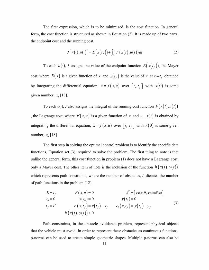
Path constraints, in the obstacle avoidance problem, represent physical objects

that the vehicle must avoid. In order to represent these obstacles as continuous functions,

p-norms can be used to create simple geometric shapes. Multiple p-norms can also be

12

used as building blocks to form more complex shapes if such shapes were needed or

desired. Equation (4) is the general form of the equation used to define the obstacles. The

center of the shape is at the location defined by cx and cy , the width of the shape is

defined by a and b , and the shape itself is defined by the value of p [12].

, i i

p p

c ci

i i

x t x y t yh x t y t

a b

(4)

Figure 3 shows the shapes derived from p-norms with p=1, 2, and 100. The square

is developed by using an exponent of p , but in practice an exponent of 100p

achieved the desired results. In each of the three examples a and b are equal to unity,

but other values are also possible. [12].

Figure 3 Unit p-norms for p =1, 2 and 100, after [12].

The strength of Pontryagin’s principle is that it avoids the curse of dimensionality,

and it solves non-linear problems without the need to linearize. The Hamiltonian, shown

in Equation (5), is used evaluate the solution of a non-linear system, and provides a

measure of the system dynamics [18].

, , : , ,TH x u F x u f x u (5)

For this problem, since there are control and path constraints the Lagrangian of

the Hamiltonian, Equation (6), will be calculated. Since there is no running cost in this

problem, ,F x u does not appear in the expression.

13

cos

, , , , : sin

,

T T

v v

H x u t v

h x t y t

(6)

In order to solve the optimal control problem Pontryagin’s principle must be

applied to the problem. A mnemonic for the necessary steps in applying the principle is

M.A.T.H., or H.-M.A.T. The “H” is the Hamiltonian, Equation (5). The “M.A.T.” is

Hamiltonian Minimization, Adjoint equation, and Transversality condition; shown in

Equation set (7).

0 Hamiltonian Minimization

Adjoint Equation

Transversality Conditionff

H

uH

tx

Et

x

(7)

where

, : Tf f fE x t E x t e x t (8)

is called the Endpoint Lagrangian [18].

All steps in the H-MAT process are required, but the Hamiltonian Minimization is

the key step for determining optimality. Pontryagin’s Minimum Principle states that for

the control function, u , to be optimal, it is necessary that for every time step, the control

function must globally minimize the Hamiltonian. So a candidate solution for the optimal

control can be derived by minimizing the Hamiltonian with respect to u (while holding

and x constant) [19]. This is done by evaluation of the partial derivative /H u .

The adjoint equations describe the dynamics for the costates [18]. These

dynamics are analyzed to generate the costate histories. The costates support the

generation of the optimal controller and thus one approach that can be used to derive the

optimal controller.

14

The transversality condition contributes any missing boundary values in the

problem. The resulting boundary value problem (BVP) is a differential equation, or rather

a system thereof, that arises from the application of Pontryagin’s Principle. The BVP has

constraints in the form of boundaries that the equations must satisfy. In order to solve the

BVP sufficient boundaries, meaning initial conditions of states or costates, equal to the

number of states and final conditions of states or costates, equal to the number of states,

must be known. If these are not given in the problem formulation they can be determined

by the transversality condition.

The application of Pontryagin’s principle for the obstacle avoidance problem is

shown in Equations (9), (10), (12), and (13):

The Hamiltonian is repeated from Equation (6):

cos

, , , , : sin

,

T T

v v

H x u t v

h x t y t

(9)

The Hamiltonian minimization condition provides:

cos sin0

0x y vH

u

(10)

From this the Karush-Kuhn-Tucker (KKT) conditions for the covectors is derived.

0 0

0 0 10

0 10

0

0

0

v

v t

for v t

v t

t

for t

t

(11)

Thus, the sign of dictates the value of the control. The costate dynamics are given by:

15

0

0

sin cos

x

y

x y

(12)

Analyzing the Transversality Condition provides the missing boundary condition on θ

1 2

1

2

Endpoint Lagrangian ,

Terminal Transversality

Conditions yields

0

f ff f f f

ff

x f

y f

f

E x t x x y x

Et

x

t

t

t

(13)

Pontryagin’s principle does not provide the solution for the problem. But by

applying the principle it is possible to generate differential equations for a new problem

that can be solved.

The obstacle avoidance problem does not lend itself to a straight forward solution.

In fact, it would be difficult, if not impossible, to solve in any timely manner without the

use of some advanced computational methods.

B. METHODOLOGY FOR SOLVING OPTIMAL CONTROL PROBLEMS

There are three broad categories of methods for solving optimal control problems:

shooting methods, collocation techniques, and pseudospectral theory [11].

1. Shooting

There are two key parts to a shooting method. The first is a means of propagating

the dynamic equations of the system given some known and some unknown initial

values. The second is a method for iterating the unknown initial values until the correct

values are found [20]. Iterating the propagation of the dynamic equations with different

initial values makes it very likely that correct initial values will be found. But it also

ensures that incorrect values for the unknown initial states and costates will also be tried.

16

Shooting methods exhibit a fundamental problem, the curse of sensitivity [20].

Initial values that are slightly off the true solution may lead to instability in the dynamic

equations propagation. In other words, a slight alteration of the initial value guess can

cause the propagated equations to “blow up.” The difference in the initial values does not

have to be very large. This can occur even in with extremely accurate guesses for the

initial values. Because of this the shooting method does not work for some problems [21].

2. Collocation

One method that does not suffer from the curse of sensitivity is the collocation

technique [20]. In collocation the time horizon from 0t to ft is discretized into N

uniform slices. Guesses for the states and costates are made for every discretized node.

The goal is to “collocate” the solution of the control problem with the behavior of the

system. This is done by approximating derivatives at each node using, for example, a

difference equation. The system of discretized generated equations is then solved

simultaneously. This introduces the disadvantage of the collocation method, the “curse of

dimensionality.” Collocation requires 22 1n N equations to be solved

simultaneously [20]. This is not the biggest disadvantage of collocation however. In order

for the collocation method to converge on a solution, there must already be reasonable

idea of the state and costate vectors of the system. For fairly well understood systems this

does not present a problem. However, for novel or poorly understood systems this can be

insurmountable. It also precludes the finding of non-intuitive solutions to the problems.

3. Pseudospectral Theory

A spectral algorithm known as the Legendre Pseudospectral (PS) method can be

used to solve nonlinear optimal control problems [11]. Unlike other methods, PS methods

use Gaussian discretization and sparsity to transform large-scale optimization problems

into a sequence of significantly smaller-scale problems. This enables improved speed and

convergence properties as compared to shooting and collocation methods [22]. Detailed

information on the Legendre PS method for solving optimal control problems is found in

reference [11], [23]

17

C. CODING AN OPTIMAL CONTROL PROBLEM IN DIDO

An optimization tool, DIDO, was used for this research in both the obstacle

avoidance and the mission planning problems. DIDO is a complete optimization tool that

is an implementation of pseudospectral methods to rapidly solve properly formulated

optimal control problems. DIDO requires no other third-party software other than

MATLAB [24].

The power of DIDO is that with knowledge of dynamics and constraints,

solutions can be produced for the optimal behavior of very complex systems. The only

requirement is that all dynamics and constraints must be expressed algebraically, and that

the problem be formulated properly. Because the elements of the problem must be

expressed algebraically, the input to DIDO is very similar to writing the problem out on

paper, which makes it a very useful and easy tool to use.

In order for the problem to be properly formulated, all the dynamics and

constraints (i.e., cost and path) must be differentiable. Also, the variables and cost

function must be scaled properly. In fact sometimes in DIDO engineering units might

cause a problem to behave badly and custom units must be developed [24]. As an

example in the case of an orbit problem, instead of using kilometers to describe the orbit

altitude the distance in earth radii could be used.

Verification and validation (V&V) of the DIDO generated solution, can be

accomplished by propagating the states generated using a propagation tool such as

MATLAB’s “ode45” solver, which uses a variable time step Runge-Kutta method, and

comparing the propagated states to the optimal control solution. If the paths match, then

the DIDO solution is valid.

Validity does not imply optimality, but DIDO also calculates the Hamiltonian at

every time step. This allows a review of the Hamiltonian to be accomplished easily in

order to ascertain optimality. The specifics of exactly how DIDO works is beyond the

scope of this research. More information on DIDO’s development, and examples

illustrating its applicability for solving optimal control problems can be found in

references [11], [25], [26].

18


19

III. THE OBSTACLE AVOIDANCE PROBLEM

While the equations in reference [12] were the basis of this work, no attempt was

made to exactly duplicate the results found therein. Rather, the intent was to study the

obstacle avoidance problem as a means of gaining understanding of potential solutions to

the mission planning problem.

A. OBSTACLES AS A PATH FUNCTION

An obstacle avoidance problem consisting of three obstacles and the vehicle

dynamics of a tricycle was set up. The problem formulation, previously shown in Chapter

II, is:

: 0 10, , : , ,

:T T

x y

v vx x y u U

0 0

Minimize , ,

Subject to cos

sin

OA

, 0,0

, 0,0

, 0

f f

f ff f

i

J x u t t

x v

y v

x y

x x y y

h x t y t

where the obstacles are defined by:

, i i

p p

c ci

i i


a b

and 1...i n for n targets.

Using the equations generated in Chapter II and entering them into DIDO an

obstacle avoidance path was calculated. The path calculated is shown in Figure 4.

20

Figure 4 Obstacle avoidance path.

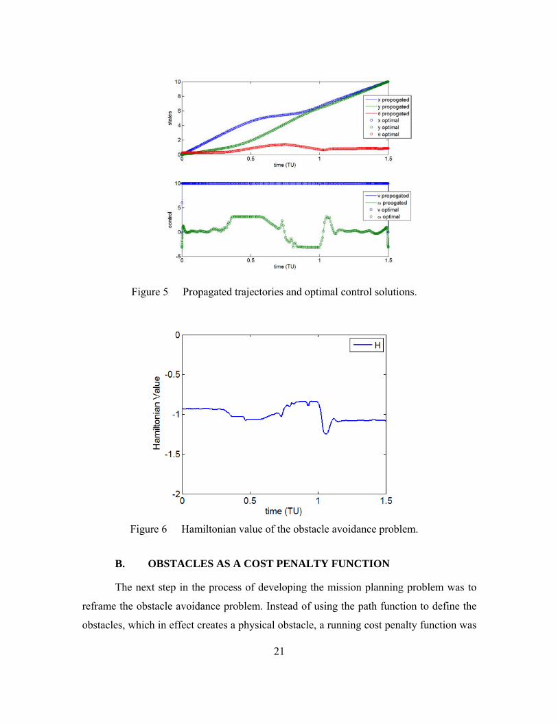
The first step in the V&V step is to compare the propagated states to the optimal

control generated states. In Figure 5 the propagated trajectories match the optimal control

generated trajectories. This shows that path is valid, i.e., it obeys the dynamics of the

system, but this test says nothing about optimality.

The most convenient check for optimality is to inspect the Hamiltonian. For a

time optimal problem, such as this one, the Hamiltonian should equal -1. The

Hamiltonian, Figure 6 , shows some variation, albeit small, from -1. An inspection of the

path in Figure 4 shows that the path intersects the corners of the objects, and this

accounts for the variation in the constancy of the Hamiltonian. There are methods to

correct for this discussed in reference [12], which will improve the Hamiltonian, and the

optimality of the path. But those methods were not pursued in order to progress to the

mission planning problem.

21

Figure 5 Propagated trajectories and optimal control solutions.

Figure 6 Hamiltonian value of the obstacle avoidance problem.

B. OBSTACLES AS A COST PENALTY FUNCTION

The next step in the process of developing the mission planning problem was to

reframe the obstacle avoidance problem. Instead of using the path function to define the

obstacles, which in effect creates a physical obstacle, a running cost penalty function was

22

written. This cost function does not prevent, in any physical sense, the vehicle from

hitting an obstacle. Instead the cost function maps a cost to violating the boundaries of

the obstacles. Thus, in order to minimize the cost, the vehicle must avoid the obstacles.

The basis for the penalty cost function is the same hi (Equation (4)) used to define

the shape and locations of the obstacles.

, i i

p p

c ci

i i


a b

(4)

This is then multiplied by -1 and used as an exponent. The final step is to take a p-

norm of the obstacle definitions so that the running cost is only calculated for the closest

obstacle to the vehicle and not for all the obstacles [12].

1

,

1

i

n ph x t y t p

Pi

F e

(14)

This new running cost, Equation (14), is used in the problem formulation while

the end cost and the path function are eliminated. This new problem formulation is shown

in Equation group (15).

: 0 10, , : , ,

:T T

x y

v vx x y u U

1 2 3

0

1, , ,

0 0

Minimize , ,

Subject to cos

OA sin

, 0,0

, 0,0

fth x t y t p h x t y t p h x t y t p p

f

t

f ff f

J x u t e e e

x v

y v

x y

x x y y

(15)

The path calculated, Figure 7, does a better job of avoiding the obstacles than

demonstrated in the previous example, but it is important to note that this is not a time

optimal problem. In fact the path takes eight time units (TU) to complete where as the

time optimal path took only 1.5 TU. Of course time could also be added to the objective

function to strike a balance between time to complete the path and obstacle avoidance.

23

Figure 7 Obstacle avoidance path with penalty cost function.

The penalty cost function demonstrates greater robustness with regard to obstacle

avoidance than the path function method; however, this robustness comes at a cost. The

path takes longer to execute than the time optimal path. Depending on the application this

cost may be acceptable.

The path is a valid path, as shown in Figure 8. There is a lot of variation in the

velocity, especially over the last two TU. However, the propagated states and controls

match the optimal.

24

Figure 8 Propagated trajectories and optimal control solutions of obstacle avoidance path with penalty cost function.

The Hamiltonian, shown in Figure 9, has a variance of 1.95x10–4. While not

absolutely constant, the variance is low enough that it can be considered constant,

showing that the path is in fact optimal. A time optimal problem, such as the previous

problem, should have a Hamiltonian value of -1, but a time free problem, such as this

one, is expected to have a value of 0. In both the previous case and this case, the

Hamiltonian value is as expected.

25

Figure 9 Hamiltonian value of obstacle avoidance path with penalty cost function.

This running penalty cost function is the key to “flipping the switch” from

obstacle avoidance to mission planning. This is because in mission planning the problem

is to “hit” as many obstacles as possible, instead of avoiding them. A modification of the

obstacle avoidance problem will be used in the mission planning problem. This insight

seems obvious, but this approach has never been documented in the literature. The result,

suggested first by Professor Ron Proulx [27], is therefore a fundamental breakthrough

that allows optimal control techniques to be used directly to solve what is typically

known as a very hard problem.

26


27

IV. THE MISSION PLANNING PROBLEM

The goal of this research is to develop an algorithm based on optimal control

concepts for mission planning and control in target rich environments. The algorithm is

based on “flipping” the obstacle avoidance problem. The goals of the algorithm are to:

incentivize target selection, and penalize loitering, while functioning in an environment

constrained by time and vehicle dynamics.

Many existing mission planning techniques do not include detailed dynamics of

the vehicle, despite the fact that dynamics fundamentally governs what can and cannot be

done. Most techniques involve a two-step process; first, a scheduler and second, a path

planner. The scheduler uses limited, if any, knowledge of the vehicle dynamics, and

determines a candidate subset of targets to be selected. Then the path planner checks the

feasibility of the schedule. If the plan is infeasible the two-step process is repeated with

fewer targets or by using a different set of targets. The solution thus derived will almost

always be sub-optimal. Optimal control provides a framework for a single step planning

process that uses complete knowledge of vehicle dynamics to select the optimal target

subset.

Ideally, the algorithm will design a plan that allows all targets in a data set to be

collected. If all targets cannot be visited, then a path through the data set that maximizes

performance will be selected. If all targets are of the same priority, then the optimal path

will visit the largest number of targets possible. If the targets are of different priorities,

than the algorithm will prioritize visits to the higher value targets.

A. VEHICLE DYNAMICS

The ultimate goal is to apply the algorithms generated here to very complex

dynamic systems such as UAVs and satellites, including not only the dynamics of the

vehicle, but also the dynamics of the sensors on board. However, since the ideas are new

and untested, a simple problem is used to prove out the concepts. For this purpose the

nonlinear kinematics of the tricycle, the same introduced in Chapter II, are ideal.

28

The tricycle has two rear wheels and one front steering wheel, which provides the

driving power [12]. The states of the vehicle are shown in Equation (16)

3

x

x y

(16)

where x and y are the position of the steering wheel and is the heading angle of the

vehicle with respect to the horizontal axis.

The bounds of x and y define the area the tricycle can operate. The bounds of θ

define how far the vehicle can turn. The state bounds are shown in Equation (17).

min max

min max

min max

: 0, 10

: 0, 10

: ,

x x x

y y y

(17)

The controls for the tricycle, shown in (18), are velocity v and steering rate .

v

u

where

: 0 10

:

v v tu U

t

(18)

Both controls encompass continuous ranges, allowing for variable velocity and

heading change rates. The velocity lower limit does not allow the tricycle to travel in

reverse, but steering allows the tricycle to reverse its direction of travel.

The kinematics of the tricycle system are:

cos

sin

x v

x y v

(19)

The initial states, final states, costates, and endpoints are:

, , , 0

Ti i io ox t x y t (20)

, , ,Tf f f f

f fx t x y t t (21)

29

B. TARGET DEFINITION

Before an algorithm for path selection can be developed, there must be a

framework for translating the target locations, and properties as appropriate, into a form

that can be used as part of the problem formulation [16]. This framework achieves the

goal of “flipping” the obstacle avoidance problem into a mission planning problem using

the ideas outlined in this section. In their simplest form target locations can be defined

using a Cartesian coordinate system.

Let 1 2, ,...,TN ,be the abstract locations of the targets. An example target set is:

3 3

6 3

4 6

7 6

(22)

This target set is shown in Figure 10.

Figure 10 Example targets in a field.

30

For mission planning the location of the target points must be differentiated from

the rest of the field. The first step in this process is to define the Kronecker d-function of

the targets:

1,

0i

ii

if

if

(23)

The Kronecker delta functions of unit length define an indicator function of the

targets. An indicator function, L̂ , is a function in probability where in a sample space

an event takes the value of 1 where the event occurs and 0 where it does not occur. In this

case the sample space is the target field and the events are the target points in the field.

The indicator function in Equation (24) generates unit impulses, at the location of the

targets, as shown in Figure 11.

1

ˆ : ,TN

ii

L

(24)

Figure 11 Indicator function plot of target set L̂ .

L̂

31

If the targets have different priorities it will be necessary to differentiate them

from one another. Let is , 1... Ti N i=1…NT be the priorities for each target. Priorities

for the example target set might be:

3 10 1 5T

s (25)

A priority scaled indicator function is now defined by

1

ˆ : ,TN

p i ii

L s

(26)

The priorities may be a function of time or other variables si º si (t…), as long as

they are related, consistent, and only vary by scale across the target set. As shown in

Figure 12, the prioritized indicator function scales the unit impulses according to the

assigned priorities.

Figure 12 Priority scaled indicator function plot of set ˆpL .

ˆpL

32

Let Nxx be the state vector of a vehicle, and let x be defined or given.

Knowing both the state vector of the vehicle and the target set, the score function, s x ,

can be defined:

1

: ,TN

i ii

s x L x s x

(27)

Having defined a procedure for relating the instantaneous position of the vehicle

to a target location, the mission planning problem has been successfully remapped from

the original obstacle avoidance problem. The issue now is how to maximize the total

score along a path x t , subject to constraints.

An appropriate objective function for maximization is therefore:

f

o

t

t

J S x t dt (28)

The goal in optimization is to minimize the cost function. The goal of the mission

planning problem, as defined here, is to maximize the score function. Since the cost

function is the score as a function of time, these two goals seem contradictory. But by

using appropriate gains the absolute value of the score function can be maximized while

the cost function is minimized. In other words, by multiplying the objective function

by -1, the objective function for minimization is:

f

o

t

t

J S x t dt (29)

The plot of the Dirac-d function, as shown in Figure 13, has zero width and an

infinite height. Thus it is not scalable. The area under the plot equals one, but it is not a

smooth curve, and therefore cannot be used for the mission planning problem.

33

Figure 13 Dirac-d function

So, instead we could try to use the Kronecker delta in order to produce the unit

indicator function. The Kronecker delta is a discontinuous, non-differentiable function,

and so is not compatible with optimal control. Thus, as it’s formulated here s x t is

non-differentiable. Hence, we are forced to find smooth approximations to the d-function

in calculating the objective function. In choosing an approximation to the delta function

we only need to ensure we meet the following property of the Dirac delta function:

1d (30)

Various Dirac delta approximations could be used. Some options for

approximations are: sinc, and exponential (Gaussian) functions.

Figure 14 shows a normalized sinc function centered at 5 on the x axis. The sinc

function is given as:

1: sinc

(31)

34

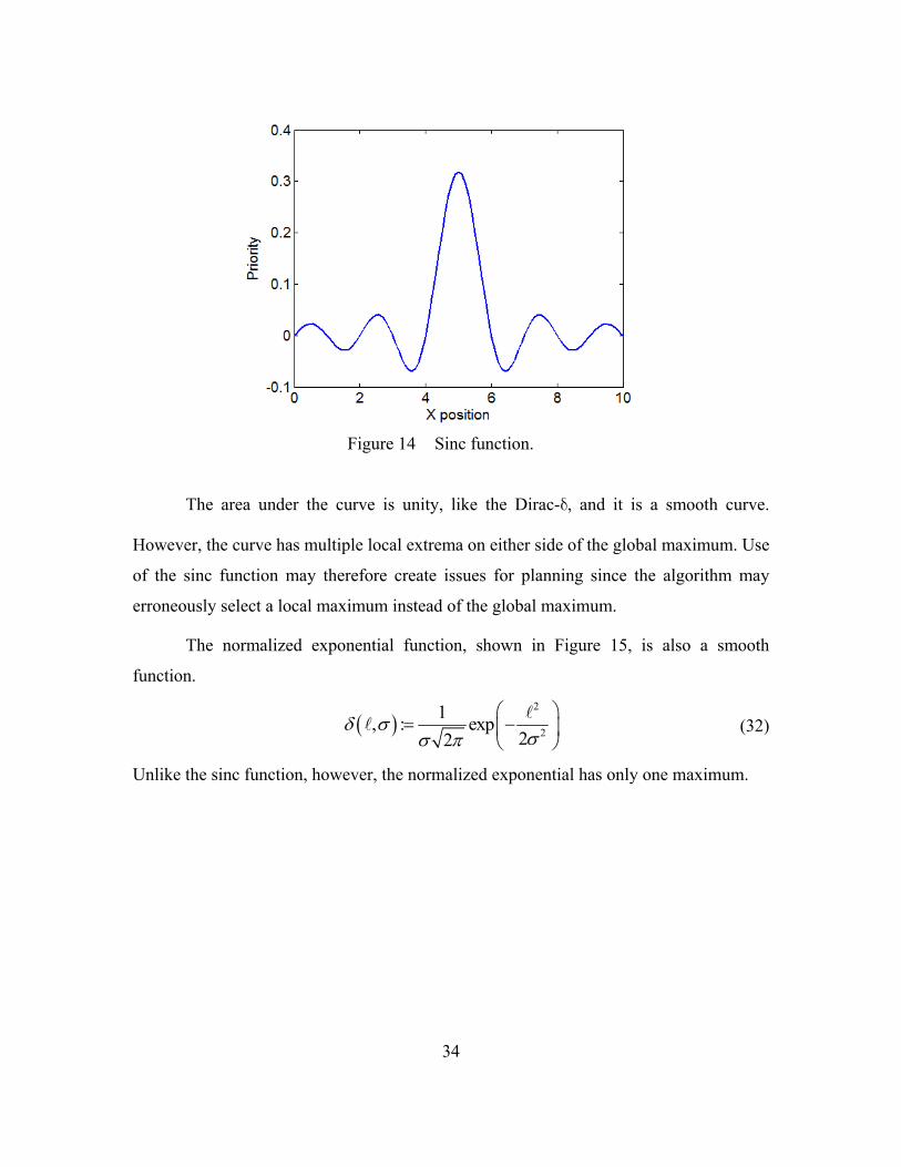
Figure 14 Sinc function.

The area under the curve is unity, like the Dirac-d, and it is a smooth curve.

However, the curve has multiple local extrema on either side of the global maximum. Use

of the sinc function may therefore create issues for planning since the algorithm may

erroneously select a local maximum instead of the global maximum.

The normalized exponential function, shown in Figure 15, is also a smooth

function.

2

2

1, : exp

22

(32)

Unlike the sinc function, however, the normalized exponential has only one maximum.

35

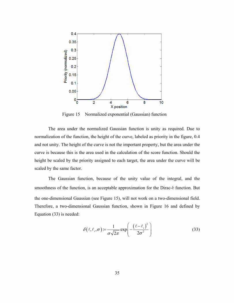
Figure 15 Normalized exponential (Gaussian) function

The area under the normalized Gaussian function is unity as required. Due to

normalization of the function, the height of the curve, labeled as priority in the figure, 0.4

and not unity. The height of the curve is not the important property, but the area under the

curve is because this is the area used in the calculation of the score function. Should the

height be scaled by the priority assigned to each target, the area under the curve will be

scaled by the same factor.

The Gaussian function, because of the unity value of the integral, and the

smoothness of the function, is an acceptable approximation for the Dirac-d function. But

the one-dimensional Gaussian (see Figure 15), will not work on a two-dimensional field.

Therefore, a two-dimensional Gaussian function, shown in Figure 16 and defined by

Equation (33) is needed:

2

2

1, , : exp

22i

i

(33)

36

Figure 16 Two-dimensional normalized Gaussian function

The potential field defined by the normalized Gaussian function for the target set

and priorities listed below is shown in Figure 17 and defined by Equation (35).

Target set () and priorities (s) are:

3 3 3

6 3 10

4 6 1

7 6 5

s

(34)

2 24

2 21

1exp

2 22i i

p ii

x x y yL s

(35)

where

1 (36)

37

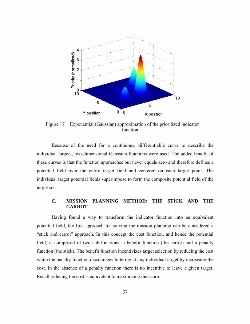
Figure 17 Exponential (Gaussian) approximation of the prioritized indicator function.

Because of the need for a continuous, differentiable curve to describe the

individual targets, two-dimensional Gaussian functions were used. The added benefit of

these curves is that the function approaches but never equals zero and therefore defines a

potential field over the entire target field and centered on each target point. The

individual target potential fields superimpose to form the composite potential field of the

target set.

C. MISSION PLANNING METHOD: THE STICK AND THE CARROT

Having found a way to transform the indicator function into an equivalent

potential field, the first approach for solving the mission planning can be considered a

“stick and carrot” approach. In this concept the cost function, and hence the potential

field, is comprised of two sub-functions: a benefit function (the carrot) and a penalty

function (the stick). The benefit function incentivizes target selection by reducing the cost

while the penalty function discourages loitering at any individual target by increasing the

cost. In the absence of a penalty function there is no incentive to leave a given target.

Recall reducing the cost is equivalent to maximizing the score.

38

With only the “carrot,” the highest value target will be selected and the vehicle

will tend to loiter at that target in order to collect the maximum benefit in the time

available. The target will be left only when the amount of time remaining represents the

time needed to travel to the end point.

The purpose of the “stick” is to prevent loitering at any one target by assigning a

penalty for loitering in the vicinity of a target for too long. The penalty is calculated the

in the same manner as the benefit, but with a smaller value to ensure there is always some

benefit that can be accumulated at every target location. This penalty both prevents

loitering and incentivizes further target selection by moving the vehicle off of the

currently selected target so that it can be allocated to the other targets. The key is to find a

balance between the two sub-functions so that the objective, maximizing score without

loiter, is achieved. A representative approximation of the prioritized indicator function of

the benefit and penalty for a single target is shown below in Figure 18.

Figure 18 Exponential (Gaussian) approximation of the prioritized indicator function of the benefit (a) and penalty (b) for a single target.

39

V. SPARSE TARGET FIELD

In this chapter, the concept of the stick and carrot approach described in the last

chapter is explored for a sparse target field. A sparse target field is defined as one in

which, based on time constraints, all targets can be visited at least once by the vehicle

within the allocated time window. Figure 19 shows an example sparse target field with

four targets.

Figure 19 Benefit function for sparse target field.

First, we examine planning in a sparse field where all targets have the same

priority. The behavior of the optimal control based mission planning approach is explored

for a prioritized sparse field next. In the next chapter, we explore the behavior of the

approach in a target rich field (i.e., a target field in which all targets cannot be visited

within the time window allocated).

A. TARGETS WITH EQUAL PRIORITY

Since, by definition, the targets in a sparse field can all be visited at least once, the

optimal plan through targets each having the same priority will depend only on the

vehicle dynamics and the particular arrangement of the targets in the field.

40

1. Setting Up the Problem

As stated earlier, to optimize the selected path it is necessary to minimize cost

function:

, ,f

o

t

f

t

J x u t F x t dt (37)

For the mission planning problem;

Gain GainF x t B Benefit P Penalty (38)

A gain (BGain) is applied to the Benefit function to incentivize target selection

while a separate gain (PGain) is applied to the Penalty function to dis-incentivize

loitering at any individual target. Since the goal is to minimize the cost function, BGain is

a negative number and PGain is a positive number. A key challenge is to find a balance

between the two gains so that the goal of maximizing target selection without loiter, is

achieved.

It was found empirically that the gains that work best are related to each other by

a ratio of BGain : PGain =-2:1. The best results achieved, based on analyzing the solutions

obtained, were achieved using the lowest gains. This had the desirable effect of properly

scaling the cost function.

With the ideal gains(38) can be rewritten as:

2 Gain GainF x t P Benefit P Penalty (39)

Through trial and error, the numerical values of the gains found to work best are:

0.03125

2 0.0625Gain

Gain Gain

P

B P

(40)

The fulcrum on the mission objective is that the absolute value of the benefit at

the target must exceed the penalty or else the vehicle will never arrive at the target. But

the penalty must be large enough that the vehicle does not linger at, or in the vicinity of,

the target in an attempt to maximize the score. This balance is achieved by the gains

applied to both the benefit and penalty sub-functions of the cost function.

41

If the benefit and penalty functions are calculated uniformly over the entire target

field the effect is no different than using the composite cost function. Thus, the penalty

must be subsumed into the benefit function and reduce its value uniformly depending

on the distance of the vehicle from the target.

In order to incentivize target selection and discourage loitering, it is necessary to

differentiate the application of the benefit and penalty function to the path selected. The

benefit at any point in the field is calculated as the sum of the benefits as a function of the

distance of the target from each target in the target set. In this manner the benefit derived

from the entire target field at all points is considered in selection of the optimal vehicle

path. The vehicle can “sense” all the targets in the target field and their relative benefit

even while at a different target in the target set.

The penalty, on the other hand, is calculated as a function of the distance of the

vehicle from only the nearest target to the vehicle. In this manner the vehicle is

encouraged to depart the current target after the maximum benefit has been collected at

that target point. This is achieved by taking a p-norm of the penalty function.

The cost function may therefore be written as:

2 2

1

2 2i i i ix x y y x x y y p

p

Gain GainF x t B e P e

(41)

And, for the n-target problem:

2 2

1

2 2

1 1

i i i ix x y y x x y y pn n

Gain Gaini i

F x t B e P e

(42)

Where x and y are the vehicle position, ix and iy are the individual target

locations, and is the standard deviation of the two-dimensional Gaussian function used

to define the target location (see Section IV.B.).

As p in Equation (42) approaches a value of it will select the maximum value

in the set, which in this case will be the penalty from the target closest to the path at any

point. In practice any p value greater than or equal to 100 will achieve the desired results.

42

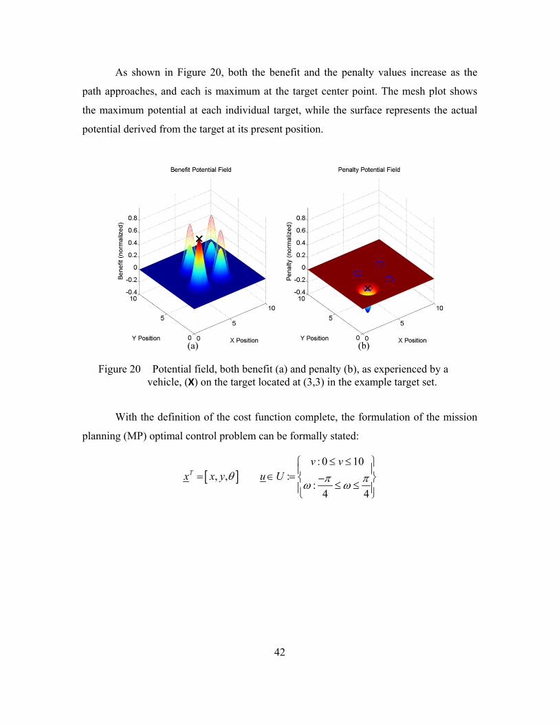
As shown in Figure 20, both the benefit and the penalty values increase as the

path approaches, and each is maximum at the target center point. The mesh plot shows

the maximum potential at each individual target, while the surface represents the actual

potential derived from the target at its present position.

Figure 20 Potential field, both benefit (a) and penalty (b), as experienced by a vehicle, (X) on the target located at (3,3) in the example target set.

With the definition of the cost function complete, the formulation of the mission

planning (MP) optimal control problem can be formally stated:

: 0 10

, , ::

4 4

T

v vx x y u U

43

2 2

1

2 2

1 10

0 0

Minimize , ,

Subject to cos

sin

, 0,0

, 0,0

i i i ifx x y y x x y y pt n n

f Gain Gaini i

f ff f

J x u t B e P e dt

x v

y v

x y

x x y y

(43)

Application of Pontryagin’s principle to the optimal control problem gives the

following [14], [16], [19].

The Hamiltonian is defined as:

cos

, , , sinT

v

H x u t F x t v

(44)

Tx ywhere

The Lagrangian of the Hamiltonian includes the controls:

cos

, , , , sinT T

vv

H x u t F x t v

(45)

Tvwhere


0 cos sinx y v

H

v

(46)

0H

(47)

From this the Karush-Kuhn-Tucker (KKT) conditions for the covectors is derived.

44

0 0

0 0 10

0 10

02

02 2

02

v

v t

for v t

v t

t

for t

t

(48)

The costate dynamics are given by:

2 2

2

2 2 2 2

2 2

2

21

1

11

2 2

21

i i

i i i i

x

y y x xn

Gaini

i

px x y y x x y ypn

pGaini

i

H

x

Bx x e

Px x e e

(49)

2 2

2

2 2 2 2

2 2

2

21

1

11

2 2

21

i i

i i i i

y

y y x xn

Gaini

i

px x y y x x y yp pn

pGaini

i

H

y

By y e

Py y e e

(50)

sin cosx y (51)

Analyzing the Transversality Condition provides the missing boundary condition:

1 2

1

2

Endpoint Lagrangian , 10 10


Conditions yields

0

f f f

ff

x f

y f

f

E x x y

Et

x

t

t

t

(52)

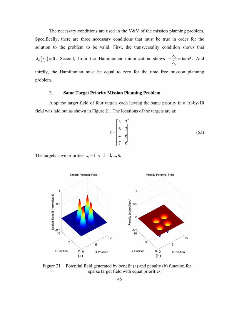
45

The necessary conditions are used in the V&V of the mission planning problem.

Specifically, there are three necessary conditions that must be true in order for the

solution to the problem to be valid. First, the transversality condition shows that

0ft . Second, from the Hamiltonian minimization shows tanx

y

. And

thirdly, the Hamiltonian must be equal to zero for the time free mission planning

problem.

2. Same Target Priority Mission Planning Problem

A sparse target field of four targets each having the same priority in a 10-by-10

field was laid out as shown in Figure 21. The locations of the targets are at:

3 3

6 3

4 6

7 6

(53)

The targets have priorities 1is 1,..., .i n

Figure 21 Potential field generated by benefit (a) and penalty (b) function for sparse target field with equal priorities.

46

The optimal path for visiting all four targets is shown in Figure 22. The target

locations are depicted using a 1-sigma radius circle centered on the target point. The

target is considered to be visited if the vehicle’s path passes within 1-sigma of the target

point. It is not necessary that the path pass directly through the target point.

Figure 22 Optimal path through sparse target field with equal priority targets.

Optimality of the solution was judged based on the Hamiltonian value. As

required by the Pontryagin principle, H t must be constant [14], as shown in Figure 23.

In this case, the variance of the Hamiltonian is 1.11x10–7, but this variance is small

enough, that the Hamiltonian can be considered numerically constant.

47

Figure 23 Plot of Hamiltonian value

The scaled states and costates are depicted in Figure 24.

Figure 24 Scaled states and costates of optimal path for sparse field with equal priority targets.

The plot of the scaled states and costates show that the states and costates are

within one order of magnitude of one another, indicating that the problem is scaled

appropriately. Also, 0ft , as required by Pontryagin’s principle, see Equation (52).

V&V of the solution, Figure 25, is accomplished by comparing the propagated states

48

against the optimal control solution. The propagated states are obtained using

MATLAB’s “ode45” solver, which uses a variable time step Runge-Kutta method to

propagate the optimal controls.


In the sparse target field it took 21.3 TU to visit all four targets. Enforcing a time

horizon less than 21.3 TU changes the nature of the problem from a sparse target field to

a target rich field. The vehicle in the latter case cannot visit all four targets because there

is not enough time. Table 1 and Figure 26 show the results of four example runs for

various time horizons: the minimum time needed to satisfy only the start and stop

conditions, the time needed to visit two targets, the time needed to visit three targets, and

the time needed to visit all four targets.

The minimum time run, Figure 26 (a), visits a target only because the target lies

on the minimum time path between the start and end points. If there were no targets lying

on the direct line between the start and end points none would have been visited.

49

Figure 26 Single priority sparse target field: (a) minimum time; (b) 2 targets; (c) 3 targets; (d) 4 targets.

As per Table 1, each path was assessed based on three metrics: mathematic

optimality, number of targets visited, and overall score accumulated by the path.

Mathematical optimality of the path was judged based on the constancy of the

Hamiltonian (a necessary condition). A target is considered visited if the path passed

within 1-σ of the target center point, as depicted by the circles surrounding the targets.

The score accumulated by the vehicle is determined by adding up the individual priorities

of the targets satisfied by the path. For single priority target fields the accumulated score

is the same as the number of targets visited. Further, no paths were considered

satisfactory if any one target was visited more than once. In other words, no target

revisits were allowed.

The purpose of the minimum time problem is to determine the smallest possible

time horizon for the problem, the time it takes to complete the path along the shortest

valid route from the start point to the end point. Thus, the total time was minimized for

that initial run and the cost function, Equation (42), was not used and the cost was not

calculated.

50

Table 1 Summary of results for mission planning in an equal priority sparse target field.

Time Cost (DU2) Hamiltonian Mean

Hamiltonian Variance

Targets Points

14.14 n/a -1.00 3.72x10–4 1 1 14.30 -0.05 -7.24x10–3 1.16x10–8 2 2 16.00 -0.07 -1.30x10–3 4.05x10–8 3 3 21.34 -0.09 -4.70x10–3 1.11x10–7 4 4

B. TARGETS WITH VARYING PRIORITIES

A sparse target field of four targets in the same locations as the previous example

was laid out. But, in this case each target was given a different priority. As shown in

Figure 27, the benefit function is scaled with the priority, but the penalty is not.

The target locations and priorities are:

3 3 3

6 3 10

4 6 1

7 6 5

s

(54)

Figure 27 Potential field generated by benefit (a) and penalty (b) function for sparse target field, different target priorities

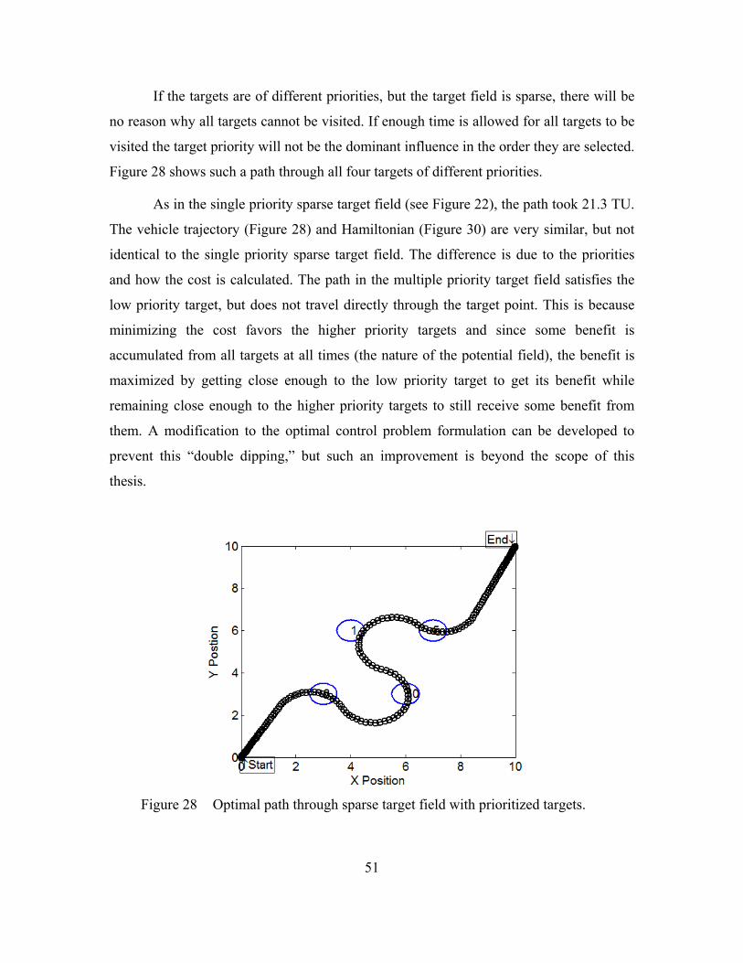
51

If the targets are of different priorities, but the target field is sparse, there will be

no reason why all targets cannot be visited. If enough time is allowed for all targets to be

visited the target priority will not be the dominant influence in the order they are selected.

Figure 28 shows such a path through all four targets of different priorities.

As in the single priority sparse target field (see Figure 22), the path took 21.3 TU.

The vehicle trajectory (Figure 28) and Hamiltonian (Figure 30) are very similar, but not

identical to the single priority sparse target field. The difference is due to the priorities

and how the cost is calculated. The path in the multiple priority target field satisfies the

low priority target, but does not travel directly through the target point. This is because

minimizing the cost favors the higher priority targets and since some benefit is

accumulated from all targets at all times (the nature of the potential field), the benefit is

maximized by getting close enough to the low priority target to get its benefit while

remaining close enough to the higher priority targets to still receive some benefit from

them. A modification to the optimal control problem formulation can be developed to

prevent this “double dipping,” but such an improvement is beyond the scope of this

thesis.

Figure 28 Optimal path through sparse target field with prioritized targets.

52

The scaled states and costates are depicted in Figure 29. This shows that the states

and costates are within one order of magnitude of one another, indicating that the

problem is scaled appropriately.

Figure 29 Scaled states and costates of optimal path

As before, optimality was judged based on the Hamiltonian of the path being

constant. As in the single priority case, the Hamiltonian shows some small variation, (see

Figure 30), but this variation is so low, that the Hamiltonian is considered constant.

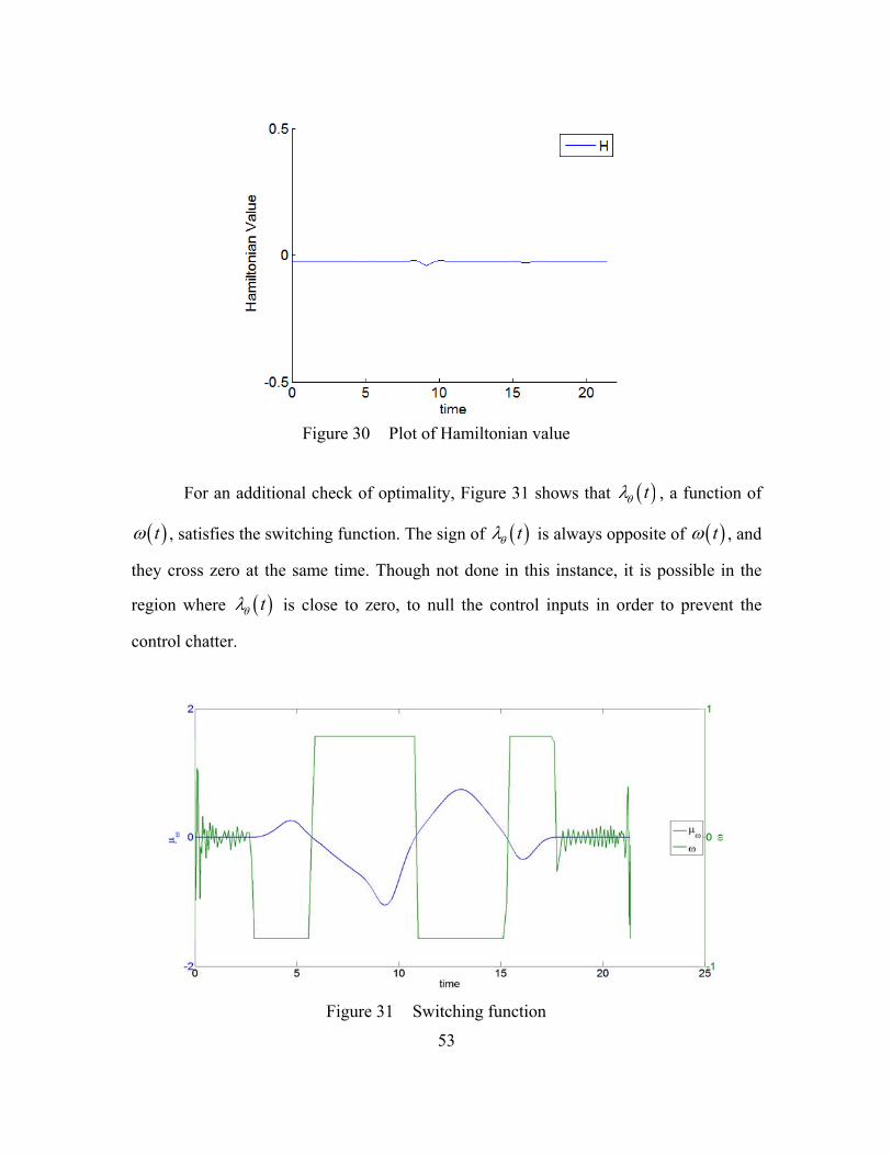
53

Figure 30 Plot of Hamiltonian value

For an additional check of optimality, Figure 31 shows that t , a function of

t , satisfies the switching function. The sign of t is always opposite of t , and

they cross zero at the same time. Though not done in this instance, it is possible in the

region where t is close to zero, to null the control inputs in order to prevent the

control chatter.

Figure 31 Switching function

54

V&V of the solution, Figure 32, is accomplished by comparing the propagated

states compared to the optimal control generated states. The propagated states are derived

as before using MATLABS “ode45” command.


When the time is constrained, the sparse target field becomes a target rich field.

With different target priorities are assigned the path selected through the field will favor

higher priority targets and the paths with differ from those selected through the single

priority target field shown in Figure 26. Figure 33 shows four paths through the multiple

priority target field: minimum time, two targets, three targets, and four targets.

As shown in Figure 26, with equal target priorities the time constrained

trajectories selected the targets closest to the start position first, then selected additional

targets in the same order. With target priority, as shown in Figure 33, the higher priority

targets are always selected first. This confirms that the developed problem formulation is

applicable for handling prioritized targets.

55

Figure 33 Multiple priority sparse target field: (a) minimum time; (b) 2 targets; (c) 3 targets; (d) 4 targets.

Table 2 Summary of results for mission planning in a multiple priority sparse target field.

Time Cost(DU2) Hamiltonian Mean

Hamiltonian Variance

Targets Points

14.14 n/a -1.00 3.72x10–4 1 3 14.89 -0.87 -2.84x10–1 2.02x10–6 2 15 15.95 -1.05 -2.01x10–2 2.20x10–6 3 18 21.34 -1.06 -2.55x10–2 5.24x10–6 4 19

C. SUMMARY

This chapter demonstrated that the optimal control based mission planning

algorithm can select a path through a sparse target field to maximize benefit. The result

also demonstrate that a dynamically feasible path can be found in a time constrained

scenario. The algorithm was also shown to have the capability to prioritize high value

target selections when it is not possible to visit all targets in a given target set. The next

chapter will expand upon the time constrained mission planning problem using a sample

target set designed to have many more targets than the can be visited in the allotted time.

56


57

VI. MISSION PLANNING IN A TARGET RICH FIELD

A target rich field is one in which all targets cannot be visited because of time

constraints. An example from practice is an imaging satellite where the mission planner

must decide which of the desired targets will be imaged, to obtain maximum benefit, in

the available imaging window. This thesis does not deal with the complex dynamics of an

imaging satellite. However, the goal of the research is to develop and validate a mission

planning process that can be adapted to just such a system.

The example target rich field used in this chapter consists of 37 targets. The target

locations were determined randomly using the MATLAB function “rand,” which

produces uniformly distributed pseudorandom numbers [28]. In this chapter, the same

problem formulation that was demonstrated to work in a sparse target field will be used

to explore solutions in a target rich field. The sparse target field, in general, can be

considered a trivial problem in that it is easier to develop a mission plan where it is

known that all targets can be visited and only the sequence needs to be determined. The

target rich field presents a more difficult planning problem since not all the targets can be

visited and the subset which produces the greatest benefit must be selected while the

others are ignored. And the target rich problem is one that is closer to real world

problems.

A. TARGETS WITH EQUAL PRIORITY

The potential fields described by the Gaussian surfaces for both the benefit and

penalty functions for a field of targets of the same priority is shown in Figure 34. Because

of the 2-to-1 ratio of the benefit to penalty (see Section V.A.1), the peaks of the benefit

function are twice as high as the peaks of the penalty function.

58

Figure 34 Potential field generated by benefit (a) and penalty (b) function for target rich field with equal priorities.

In the sparse target field, shown in Figure 21, and repeated in Figure 35, each

target is sufficiently distanced from the other targets to generate a distinct peak in the

potential field. In the target rich field, on the other hand, the targets are close enough to

other targets to cause aggregate, non-discrete, peaks in the potential field, as shown in

Figure 34. The maximum heights of these aggregate peaks are higher than the individual

peaks in the sparse target field. This suggests that there are clusters of targets with large

aggregate benefit even though the individual targets have the same priorities. It is

expected that these clusters will be revisited over individual targets in order to maximize

the benefit, subject to the capabilities of the vehicle.

59

Figure 35 Potential field generated by benefit (a) and penalty (b) function for sparse target field with equal priorities.

The path shown in Figure 36 is the optimal path through the equal priority target

rich field. This path is an extremal path through this target rich field because it satisfies

all the necessary conditions of optimality as discussed in Chapter V. The path does not

pass through the center of some targets, but as stated earlier, passage within 1-σ of the

target point is sufficient to count as a target visit.

60

Figure 36 Optimal path in a target rich field with equal priority targets.

The presence of aggregate, local, maxima in the potential field explain two

aspects of the path selected. First, these aggregate peaks are the reason why the path is

attracted to a cluster of targets as opposed to individual targets. Second, the aggregate

peak explains why the path tends to pass through the center of a cluster of targets, circled

in red in the lower right corner of Figure 36, instead of through the center of the

individual targets in the target cluster. The path actually passes directly through the center

of the local aggregate peak in the benefit potential field, because this is the locus of

maximum local benefit. A modification of the problem formulation may be able to

prevent these aggregate benefit potentials or the path steering caused by them, and such

improvements could be useful in certain applications and are thus suggested as future

work.

For the target rich field the time is always constrained. Therefore, with equal

target priorities the path through the field will visit as many targets as possible in the

allotted time. Figure 37 illustrates this point by showing four paths through the single

priority target field, each for a different allotted time horizon.

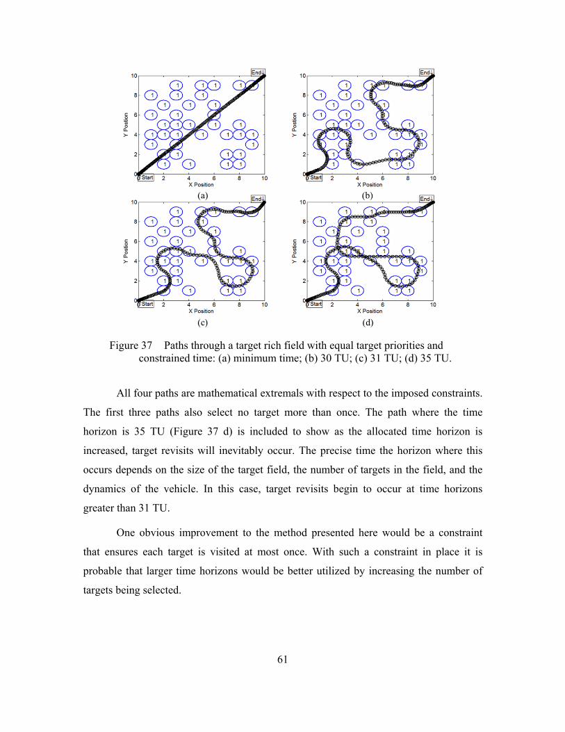
61

Figure 37 Paths through a target rich field with equal target priorities and constrained time: (a) minimum time; (b) 30 TU; (c) 31 TU; (d) 35 TU.

All four paths are mathematical extremals with respect to the imposed constraints.

The first three paths also select no target more than once. The path where the time

horizon is 35 TU (Figure 37 d) is included to show as the allocated time horizon is

increased, target revisits will inevitably occur. The precise time the horizon where this

occurs depends on the size of the target field, the number of targets in the field, and the

dynamics of the vehicle. In this case, target revisits begin to occur at time horizons

greater than 31 TU.

One obvious improvement to the method presented here would be a constraint

that ensures each target is visited at most once. With such a constraint in place it is

probable that larger time horizons would be better utilized by increasing the number of

targets being selected.

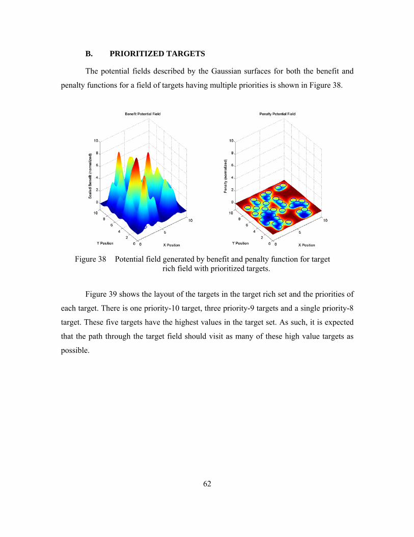
62

B. PRIORITIZED TARGETS

The potential fields described by the Gaussian surfaces for both the benefit and

penalty functions for a field of targets having multiple priorities is shown in Figure 38.

Figure 38 Potential field generated by benefit and penalty function for target rich field with prioritized targets.

Figure 39 shows the layout of the targets in the target rich set and the priorities of

each target. There is one priority-10 target, three priority-9 targets and a single priority-8

target. These five targets have the highest values in the target set. As such, it is expected

that the path through the target field should visit as many of these high value targets as

possible.

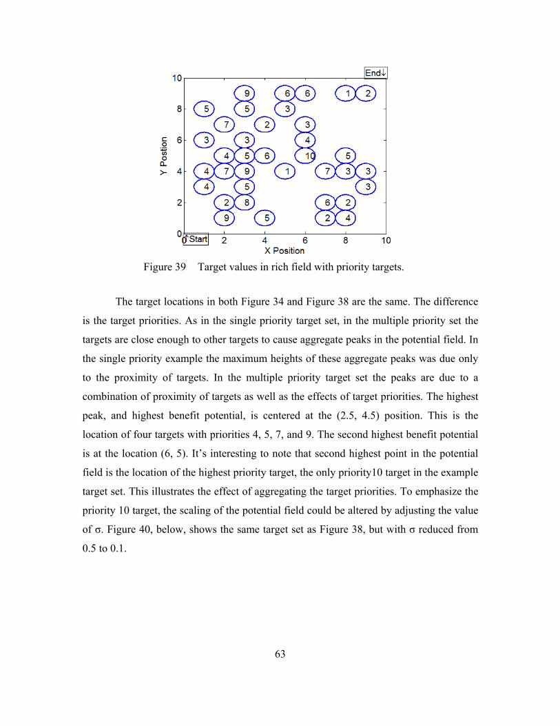
63

Figure 39 Target values in rich field with priority targets.

The target locations in both Figure 34 and Figure 38 are the same. The difference

is the target priorities. As in the single priority target set, in the multiple priority set the

targets are close enough to other targets to cause aggregate peaks in the potential field. In

the single priority example the maximum heights of these aggregate peaks was due only

to the proximity of targets. In the multiple priority target set the peaks are due to a

combination of proximity of targets as well as the effects of target priorities. The highest

peak, and highest benefit potential, is centered at the (2.5, 4.5) position. This is the

location of four targets with priorities 4, 5, 7, and 9. The second highest benefit potential

is at the location (6, 5). It’s interesting to note that second highest point in the potential

field is the location of the highest priority target, the only priority10 target in the example

target set. This illustrates the effect of aggregating the target priorities. To emphasize the

priority 10 target, the scaling of the potential field could be altered by adjusting the value

of σ. Figure 40, below, shows the same target set as Figure 38, but with σ reduced from

0.5 to 0.1.

64

Figure 40 Potential field generated by benefit and penalty function for target rich field with prioritized targets with σ = 0.1.

Given that the algorithm is designed to seek the highest benefit potential, it is

expected that when 0.5 , the algorithm will prioritize the cluster of higher value

targets over the single high priority target. Solutions to the problem are now explored.

1. Seeding the Algorithm

Now that the number of targets in the field have been significantly increased, it is

necessary to discuss how the algorithm can be initialized using a seed. The seed is used

by the mission planning algorithm as the first attempt at the ideal plan. Because of this,

seeding could affect the final path selected by the planning algorithm unless the solution

is globally convergent. In the sparse target field no difference was noted with a change in

the seed, but with the large number of targets in the example target rich field the seed

could make a difference. Ideally, the seed should not impact the solution. If it does, the

solution may only converge locally. If the seed does not change the plan, the algorithm is

robust to any presorting of the targets and thus can obtain a global minimum. This

robustness is desirable since human intuition (as inserted in the seed) does not, in general,

lead to the maximum benefit.

The target set and the priorities were generated randomly. The target set could be

presented for the mission planning algorithm in the same random order. Instead, the

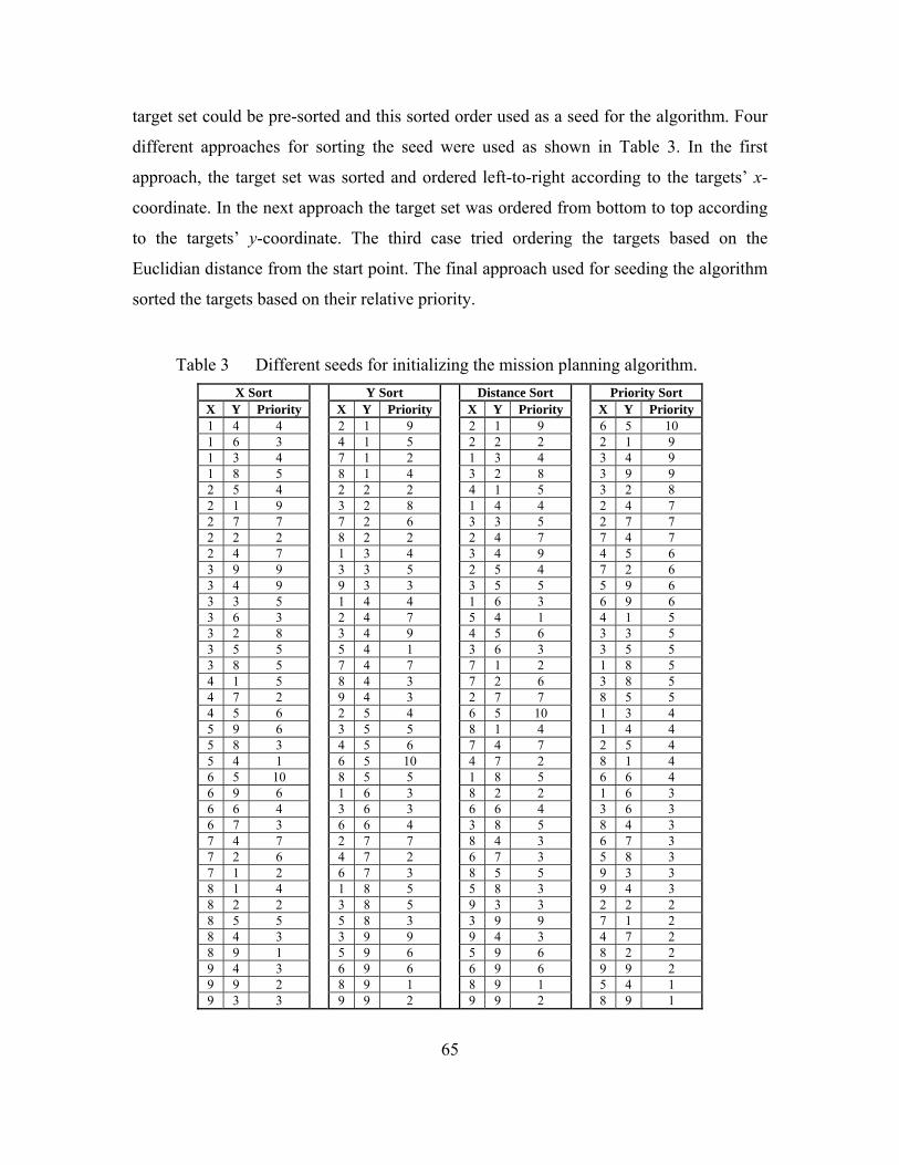
65

target set could be pre-sorted and this sorted order used as a seed for the algorithm. Four

different approaches for sorting the seed were used as shown in Table 3. In the first

approach, the target set was sorted and ordered left-to-right according to the targets’ x-

coordinate. In the next approach the target set was ordered from bottom to top according

to the targets’ y-coordinate. The third case tried ordering the targets based on the

Euclidian distance from the start point. The final approach used for seeding the algorithm

sorted the targets based on their relative priority.

Table 3 Different seeds for initializing the mission planning algorithm.

X Sort Y Sort Distance Sort Priority Sort X Y Priority X Y Priority X Y Priority X Y Priority 1 4 4 2 1 9 2 1 9 6 5 10 1 6 3 4 1 5 2 2 2 2 1 9 1 3 4 7 1 2 1 3 4 3 4 9 1 8 5 8 1 4 3 2 8 3 9 9 2 5 4 2 2 2 4 1 5 3 2 8 2 1 9 3 2 8 1 4 4 2 4 7 2 7 7 7 2 6 3 3 5 2 7 7 2 2 2 8 2 2 2 4 7 7 4 7 2 4 7 1 3 4 3 4 9 4 5 6 3 9 9 3 3 5 2 5 4 7 2 6 3 4 9 9 3 3 3 5 5 5 9 6 3 3 5 1 4 4 1 6 3 6 9 6 3 6 3 2 4 7 5 4 1 4 1 5 3 2 8 3 4 9 4 5 6 3 3 5 3 5 5 5 4 1 3 6 3 3 5 5 3 8 5 7 4 7 7 1 2 1 8 5 4 1 5 8 4 3 7 2 6 3 8 5 4 7 2 9 4 3 2 7 7 8 5 5 4 5 6 2 5 4 6 5 10 1 3 4 5 9 6 3 5 5 8 1 4 1 4 4 5 8 3 4 5 6 7 4 7 2 5 4 5 4 1 6 5 10 4 7 2 8 1 4 6 5 10 8 5 5 1 8 5 6 6 4 6 9 6 1 6 3 8 2 2 1 6 3 6 6 4 3 6 3 6 6 4 3 6 3 6 7 3 6 6 4 3 8 5 8 4 3 7 4 7 2 7 7 8 4 3 6 7 3 7 2 6 4 7 2 6 7 3 5 8 3 7 1 2 6 7 3 8 5 5 9 3 3 8 1 4 1 8 5 5 8 3 9 4 3 8 2 2 3 8 5 9 3 3 2 2 2 8 5 5 5 8 3 3 9 9 7 1 2 8 4 3 3 9 9 9 4 3 4 7 2 8 9 1 5 9 6 5 9 6 8 2 2 9 4 3 6 9 6 6 9 6 9 9 2 9 9 2 8 9 1 8 9 1 5 4 1 9 3 3 9 9 2 9 9 2 8 9 1

66

To evaluate the robustness of the algorithm, the different seeds given in Table 3

were each used to generate paths for time horizons from 15 TU to 50 TU in increments of

1 TU. The results are shown in Figure 41. The results of the paths over all 36 time

horizons are plotted together to evaluate two conditions: whether there is a particular path

that gets selected more often, and to determine if different seeding algorithms produced

different paths overall. This latter test allows the robustness of the algorithm to be

evaluated.

Figure 41 Paths for varying time horizons using different seeds: (a) target set sorted on X position; (b) target set sorted on Y position; (c) target set sorted by Euclidian distance from start point; (d) target set sorted by

priority.

The results show that there is no single optimal path over all time horizons.

However, there are some trends indicated by the more heavily travelled tracks. At each

time horizon, the paths traversed by the vehicle are essentially the same. This indicates

the consistency of the algorithm. More importantly, no seed outperformed any other. This

shows that the mission planning algorithm is robust against changes in the seed.

Therefore, in using the algorithm, no prior knowledge of the ideal path is required in

order to maximize the score. This indicates that the algorithm can globally maximize the

benefit. If the algorithm was sensitive to different seed sequences, only local maxima can

67

be found and the mission planner would have to have some idea of the ideal path, or

applying the path planning algorithm iteratively, in order to find the best plan. This would

de-value the advantages of the proposed optimal control based approach for solving

mission planning problems.

2. Solutions in a Prioritized Target Rich Field

Figure 42 shows an example path through the target rich multiple priority field

given a time horizon of 30 TU. The path is notably different than the equal priority path

over the same horizon (see Figure 36).

Figure 42 Paths in target rich field: prioritized targets (black); equal priority targets (red).

By chance, the higher priority targets fall in or near the groupings of targets that

the path through the equal priority field already favored. This is due to the locations of

the targets and the clusters of targets common to both target sets. In the equal priority

target fields all targets have the same priority (i.e., no target is more favored than any

other single target). The differences in the two paths is due to the fact that the equal

priority path maximizes the score by selecting the most targets possible and the

prioritized path maximizes the score by prioritizing higher priority targets while selecting

68

as many targets as possible. The equal priority target path selects 21 targets while the

prioritized target path selects 18 targets. While the prioritized path did not select as many

targets (as expected) it visited all four of the highest priority targets in the target set. It

also achieved a higher score function, or a smaller cost, than the single priority target.

The cost for the multiple-priority path was -9.15 the single priority path was -1.28.

With multiple target priorities the optimal path through the field will select targets

to maximize the benefit function as much as possible in the allotted time. Figure 43

shows how the path varies as a function of the time horizon. Four paths through the

multiple priority target field are shown in Figure 42: minimum time, 17 TU, 25 TU, and

30 TU.

Figure 43 Multiple priority target rich field: (a) minimum time; (b) 17 TU; (c) 25 TU; (d) 30 TU.

All four paths are mathematically optimal and none of the paths visit any target

more than once. As expected, all paths other than the minimum time path prioritize the

69

high value targets. Of the five high priority targets the 17 TU path selects three, while the

25 TU and 30 TU paths each select four. The 30 TU path only visits two more targets

than the 25 TU path, but it scores 19 more points by selecting the additional visited

targets to be higher priority ones. Beyond 30 TU revisits begin to occur, which does not

increase the score.

C. CONCLUSION

In this chapter, the same problem formulation that was demonstrated to work in a

sparse target field was validated for a target rich field. It was shown that the algorithm

can select how to visit prioritized targets given an allotted time horizon and it

simultaneously provides dynamically feasible paths.

One important difference between the sparse target field and the target rich field

is that the proximity and number of targets causes aggregate, non-discrete, peaks in the

potential field. This has the effect of causing the path to drive through the center of the

aggregate peak and not through the individual targets. The aggregate peaks can be

reduced or eliminated by reducing the size of the individual Gaussian surfaces

representing each target. This can be achieved by reducing the σ used. But, with a smaller

σ the attractive force of the potential field may be reduced, leading to fewer targets being

visited. Examining approaches for dealing with this issue is a logical next step.

The problem formulation was also shown to be robust to different seeding

methods. This is a very important point as it means that no prior knowledge of the

solution, even in a general sense, is needed to find the optimal path. Without formal

proof, the immunity of the algorithm to the initial seed implies that the approach is

capable of globally maximizing the benefit.

70


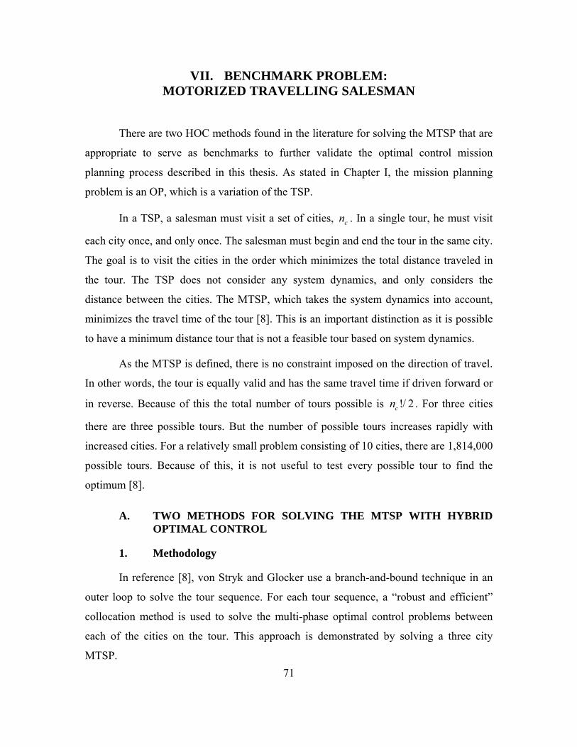
71

VII. BENCHMARK PROBLEM: MOTORIZED TRAVELLING SALESMAN

There are two HOC methods found in the literature for solving the MTSP that are

appropriate to serve as benchmarks to further validate the optimal control mission

planning process described in this thesis. As stated in Chapter I, the mission planning

problem is an OP, which is a variation of the TSP.

In a TSP, a salesman must visit a set of cities, cn . In a single tour, he must visit

each city once, and only once. The salesman must begin and end the tour in the same city.

The goal is to visit the cities in the order which minimizes the total distance traveled in

the tour. The TSP does not consider any system dynamics, and only considers the

distance between the cities. The MTSP, which takes the system dynamics into account,

minimizes the travel time of the tour [8]. This is an important distinction as it is possible

to have a minimum distance tour that is not a feasible tour based on system dynamics.

As the MTSP is defined, there is no constraint imposed on the direction of travel.

In other words, the tour is equally valid and has the same travel time if driven forward or

in reverse. Because of this the total number of tours possible is !/ 2cn . For three cities

there are three possible tours. But the number of possible tours increases rapidly with

increased cities. For a relatively small problem consisting of 10 cities, there are 1,814,000

possible tours. Because of this, it is not useful to test every possible tour to find the

optimum [8].

A. TWO METHODS FOR SOLVING THE MTSP WITH HYBRID OPTIMAL CONTROL

1. Methodology

In reference [8], von Stryk and Glocker use a branch-and-bound technique in an

outer loop to solve the tour sequence. For each tour sequence, a “robust and efficient”

collocation method is used to solve the multi-phase optimal control problems between

each of the cities on the tour. This approach is demonstrated by solving a three city

MTSP.

72

In reference [10], Conway and Chilan use a genetic algorithm (GA) for the outer

loop to determine the tour sequence and then used a Runge-Kutta parallel shooting

scheme to solve the optimal control problem. In spite of the changes in the details of the

processes used for the outer and inner loops, the previous work uses a two-stage

algorithm to solve the MTSP.

2. Problem Definition

a. System Dynamics

Both papers used the same dynamics, shown below in Equation group (55). These

dynamics are for a tricycle, similar to the dynamics used in the thesis for both the

obstacle avoidance and mission planning problems, but with a variation. In these

dynamics velocity, v , is a state variable, and not a control. Instead the control is

acceleration, .

: 1 1, , , :

: 1 1Tx x y v u U

0 0 0

0

0

cos

sin

, , 0,0,0

, , 0,0,0

,

f f

f

x v

y v

v

x y v

x y v

free

(55)

b. City Locations

In both papers, the tour started and stopped at the origin. In reference [8] there

were three cities to visit at the locations shown in Table 4.

Table 4 Locations of cities for MTSP, after [8].

City 1 2 3 x 1 2 2 y 2 2 1

73

Reference [10] added five more cities to increase the computational complexity of

the problem. The addition of only five cities increased the possible tours from three to

20,160. The modified list of city locations is shown in Table 5.

Table 5 Modified list of city locations, from [10].

City 1 2 3 4 5 6 7 8 x 1 2 2 5 10 10 5 7 y 2 2 1 10 10 5 5 7

3. Problem Solution

In reference [8], with only three cities, the authors could solve each of the

possible three tours. Two of the tours, because of system dynamics, had two possible

solutions each, for a total of five tours to consider. Each tour is shown in Figure 44. This

demonstrated the validity of the technique for establishing feasible maneuvers. The

optimal path was determined to be C1,C2,C3, specifically route (a1). The tour takes 7.617

TU to complete [8]. Since each possible solution could be enumerated, the robustness of

the branch-and-bound outer loop could not be tested.

Figure 44 The five minimum time solution candidates obtained for the MTSP with three cities, from [8].

74

In reference [10], the number of cities was increased from three to eight in order

to assess the robustness of both their technique and the one introduced in reference [8].

The authors added the other cities to increase the computational complexity of the

problem (i.e., to add targets that would have properly filtered out). The additional cities

were placed in such a manner as to not affect the tour chosen when the best three city tour

was selected. The results of [10] are shown in Figure 45, along with those from [8] for

reference.

Figure 45 Optimal paths for cities 1, 2, and 3, from [10].

Using the branch-and-bound outer loop of [8], Conway and Chilan were able to

determine the optimal path after 32 iterations of the algorithm. Using the GA, it only took

22 iterations. Moreover, the optimal route took 6.98 TU to complete, a slight

improvement over [8].

B. SOLVING THE MTSP WITH THE PSEUDOSPECTRAL OPTIMAL CONTROL MISSION PLANNING METHOD

The mission planning algorithm described in this thesis was used to solve the

benchmark problem.

75

: 0.6 1, , :

: 1 1T v v

x x y u U

2 2

1

2 2

1 1

0 0

Minimize , ,

Subject to cos

sin

, 0,0

, 0,0

i i i ix x y y x x y y pn n

f Gain Gaini i

f f

J x u t B e P e

x v

y v

x y

x y

(56)

Application of Pontryagin’s principle to the optimal control problem gives the

following [14], [16], [19].

The Hamiltonian is defined as:

cos

, , , sinT

v

H x u t F x t v

(57)

Tx ywhere

The Lagrangian of the Hamiltonian includes the controls:

cos

, , , , sinT T

vv

H x u t F x t v

(58)

Tvwhere


0 cos sinx y v

H

v

(59)

0H

. (60)

From this, the Karush-Kuhn-Tucker (KKT) conditions for the covectors is derived.

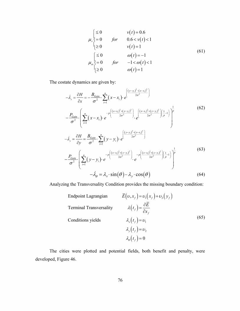
76

0 0.6

0 0.6 1

0 1

0 1

0 1 1

0 1

v

v t

for v t

v t

t

for t

t

(61)

The costate dynamics are given by:

2 2

2

2 2 2 2

2 2

2

21

1

11

2 2

21

i i

i i i i

x

y y x xn

Gaini

i

px x y y x x y ypn

pGaini

i

H

x

Bx x e

Px x e e

(62)

2 2

2

2 2 2 2

2 2

2

21

1

11

2 2

21

i i

i i i i

y

y y x xn

Gaini

i

px x y y x x y yp pn

pGaini

i

H

y

By y e

Py y e e

(63)

sin cosx y (64)

Analyzing the Transversality Condition provides the missing boundary condition:

1 2

1

2

Endpoint Lagrangian ,


Conditions yields

0

f f f

ff

x f

y f

f

E x x y

Et

x

t

t

t

(65)

The cities were plotted and potential fields, both benefit and penalty, were

developed, Figure 46.

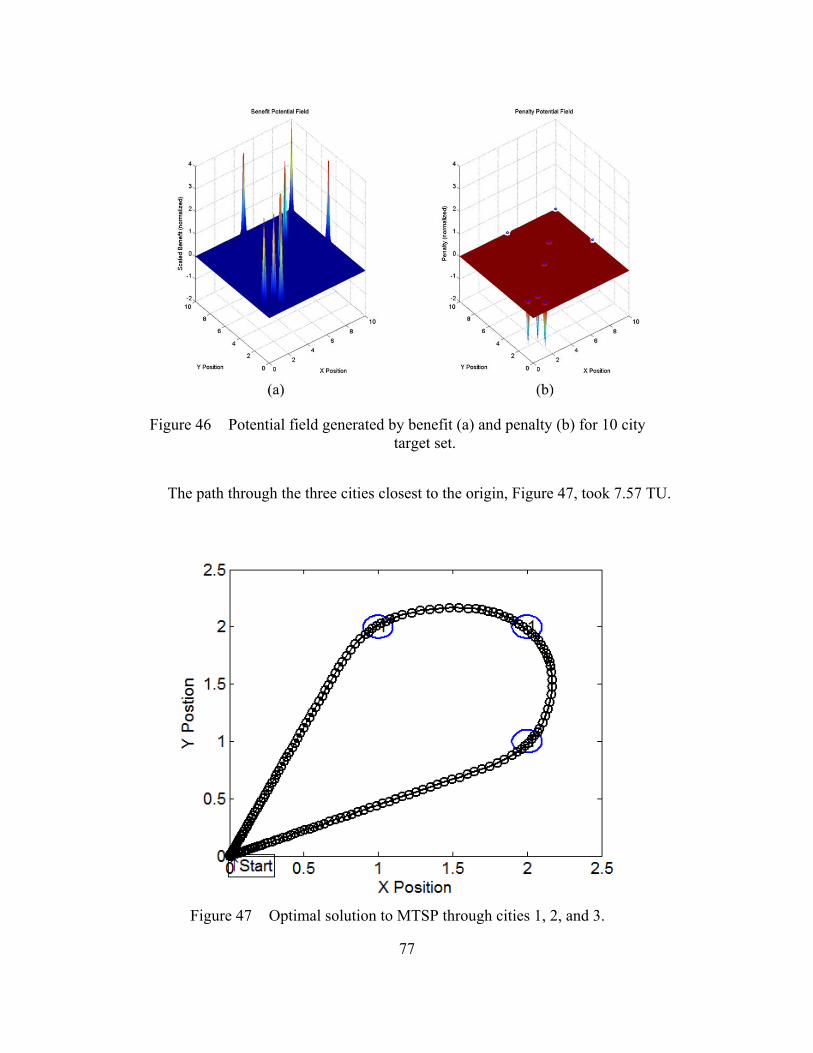
77

Figure 46 Potential field generated by benefit (a) and penalty (b) for 10 city target set.

The path through the three cities closest to the origin, Figure 47, took 7.57 TU.

Figure 47 Optimal solution to MTSP through cities 1, 2, and 3.

78

The path found by the optimal control mission planning method took longer than

Chilan and Conway, but less time than von Stryk and Glocker. This is probably due to the

slightly different dynamics used and the different methods employed to solve the optimal

control problem. The key, though, is that the mission planning process selected the same

points and the same route as the two other methods.

The scaled states and costates are depicted in Figure 48. This shows that the

problem is scaled appropriately.

Figure 48 Scaled states and costates of optimal solution to the MSTP.

The Hamiltonian, Figure 49, has a mean value of -1.0013 with a variance of

2.3x10–3. This variance is low enough that the Hamiltonian can be considered constant.

And a constant of almost -1 means that this is the time optimal solution to the MSTP.

79

Figure 49 Plot of the Hamiltonian value of MTSP.

In addition to evaluating the Hamiltonian to check for optimality, V&V of the

solution was carried out to compare the propagated states to the optimal control solution.

The results were in agreement, sot the tour is found to be dynamically feasible.

C. CONCLUSION

The optimal control mission planning algorithm developed in this thesis was able

to solve the benchmark MTSP problem without difficulty. The HOC methods require a

multi-loop, iterative process. They first determine a candidate path via discrete methods

and then solve the resulting multi-phase optimal control problem. The main challenge is

reducing the number of iterations of the outer loop.

The pseudospectral optimal control mission planning method presented here is

capable of solving the MTSP in a single step. The method will generate a feasible

solution for every given time horizon. The only iteration required is to find what time

horizon visits the number of cities desired. The only weakness, or area where

improvement would be beneficial, is a way to eliminate target revisit then, iterating the

time horizon would not be necessary. Currently, the method does not do that, but it is an

identified area of future work.

80


81

VIII. CONCLUSIONS

A. RESEARCH CONCLUSIONS

This thesis explored a new approach for mission planning problems using optimal

control. Proof of concept demonstrations illustrated the efficiency of the new ideas for an

optimal control method for solving the mission planning problem.

This thesis showed the feasibility of representing discrete, non-continuous,

targets as continuous, differentiable functions. This was done by the use of Gaussian

surfaces to create potential fields, the peaks of which are centered on each individual

target point. A cost function that incentivized target selection while also discouraging

loitering was developed. With these two ideas the problem was made suitable for

optimal control solutions using pseudospectral methods. The idea allows the mission

planning and path generation problem solvable in a single step. In all other published

work, these two steps are carried out sequentially.

B. FUTURE WORK

This work is a proof of concept. As such, there is substantial work to be done

before this method for mission planning can be applied to real world systems.

1. Target Revisit and Subtours

As the algorithm is structured now, the only way to prevent target revisit is by

limiting the time horizon. If the discrete constraint in Equation (66) could be

approximated as a continuous function, target revisit would be eliminated without the

need to limit the time horizon [4]. In the discrete case, the constraint,

1

1 2

1 2,..., 1N N

ik kji j

x x k N

(66)

where x is the path between targets and N is the number of targets, achieves the

objective.

82

A sub-tour occurs when the path described is not continuous, so the path is

actually two or more paths (not an issue with the approach used here). Equation (66)

ensures the connectivity of the path as well as ensuring that no target is visited more than

once [4].

2. Elimination of Aggregate Peaks in Potential Field

It has already been shown adjusting the value of in Equation (42) can be used

to eliminate the aggregate peaks in the potential field (see Figure 40). However, as shown

in Figure 50, with narrower Gaussian surfaces, the benefit function is not as strong across

the potential field and not as many targets are visited. There are two suggested, though

untried, solutions to this problem.

Figure 50 Comparison of path selected with single priority target sets and different values for : sparse target, 21.34 TU (a) 0.1 ; (b) 0.5 ;

target rich, 31 TU (c) 0.1 ; (d) 0.5 .

83

a. Iterative Solution with Reduced σ on Successive Steps

In this approach, a path with aggregate peaks in the potential field is found and

used as a seed for another path, this time with a smaller σ used. This could work with a

single step from 0.5 to min , or it may take several intermediate steps.

b. Dynamic σ Based on Vehicle Distance to Targets

In this approach, a minimum value, min , would be defined while the maximum

value, and all intermediate values, would be a function of the distance from the vehicle to

each target. A suggested equation for implementing this is:

2 2

min: i it c x t x y t y

(67)

3. Time Windows

In a real-world ISR mission, some targets will only be available at certain times,

or a certain amount of dwell time might be required to adequately collect the target. By

adding time windows as constraints to the mission planning process, more realistic target

sets could be developed. Each target, i, would be assigned a time window ,i iO C and

the target can only be visited in that window [4]. This introduces another set of discrete

constraints that would need to be transformed to a series of continuous constraints in

order to be used.

4. Application to More Complex Systems

This research proved the concept of the optimal control based mission planning

problem. The next logical step would be application of the method to more complex

systems such as satellites and UAVs including the dynamics of slewing sensors carried

on those systems.

84


85

LIST OF REFERENCES

[1] A. J. Newman and J. T. DeSena, “Closed-loop collaborative intelligence, surveillance, and reconnaissance resource management,” Johns Hopkins APL Technological Digest, vol. 31, no. 3, pp. 183–214, 2013.

[2] DigitalGlobe collections manager, private communication, Mar. 2012.

[3] D. L. Applegate, R. E. Bixby, V. Chvatal and W. J. Cook. (2011). The Traveling Salesman Problem: A Computational Study [Ebrary]. [Online]. Available http://site.ebrary.com/lib/nps/

[4] P. Vansteenwegen, W. Souffriau and D. Van Oudeusden, “The orienteering problem: A survey,” European Journal of Operational Research, vol. 209, pp. 1–10, 2011.

[5] B. L. Golden, L. Levy and R. Vohra, “The orienteering problem,” Naval Research Logistics, vol. 34, pp. 307–318, 1987.

[6] E. Tremblay, “Dynamic target selection using soft computing,”M.S. thesis, Dept. of Mechanical and Aerospace Engineering, Naval Postgraduate School, Monterey CA, 2014.

[7] I.-M. Chao, B. L. Golden, and E. A. Wasil, “A fast and effective heurisitic for the orienteering problem,” European Journal of Operational Research, vol. 88, pp. 475–489, 1996.

[8] O. von Stryk and M. Glocker, “Numerical mixed-integer optimal control and motorized traveling salesman problems,” European Journal of Control, vol. 35, no. 4, pp. 519–533, 2001.

[9] M. Glocker and O. von Stryk, “Hybrid optimal control of motorized travelling salesman and beyond,” in 15th IFAC World Congress on Automatic Control, Barcelona, Spain, 2002, pp. 987–992.

[10] C. Chilan and B. Conway, “A space mission automation using hybrid optimal control,” Advances in Astronautical Sciences, vol. 127, no. 1, pp. 259–276, 2007.

[11] I. M. Ross and M. Karpenko, “A review of pseudospectral optimal control: From theory to flight,” Annual Reviews in Control, vol. 36, no. 2, pp. 182–197, 2012.

[12] L. R. Lewis, “Rapid motion planning and autonomous obstacle avoidance for unmanned vehicles,” M.S.thesis, Dept. of Mechanical and Aerospace Engineering, Naval Postgraduate School, Monterey, CA, 2006.

86

[13] K. P. Bollino and L. R. Lewis, “Optimal planning and control of tactical unmanned aerial vehicles in urban environments,” presented at Unmanned Systems North America Conf., Washington, D.C., 2007.

[14] L. S. Ponryagin, V. G. Boltyanskii, R. V. Gamkrelidze, and E. F. Mischenko, The Mathematical Theory of Optimal Processes, New Yok: Interscience Publishers, 1962.

[15] R. Vinter, Optimal Control. Boston: Birkhauser, 2010.

[16] I. M. Ross, “A new approach for solving mission planning problems,” unpublished.

[17] N. K. Poulsen,( 15 January 2012). Dynamic optimization.. [Online]. Available: http://www2.imm.dtu.dk/courses/02711/DO.pdf

[18] “Spacecraft guidance and control,” class notes for AE 3830, Dept. of Mechanical and Aerospace Engineering, Naval Postgraduate School, Spring 2013.

[19] I. M. Ross, A Primer on Pontryagin’s Principle in Optimal Control, Carmel, CA: Collegiate Publishers, 2009.

[20] “Astrodynamic optimization,” class notes for AE 4850, Dept. of Mechanical and Aerospace Engineering, Naval Postgraduate School, Fall 2014.

[21] D. D. Morrison, J. D. Riley and J. F. Zancanaro, “Multiple shooting method for two-point boundary value problems,” Communications of the ACM, vol. 5, no. 12, pp. 613–614, December 1962.

[22] K. P. Bollino, L. R. Lewis, P. Sekhavat, and I. M. Ross, “Pseudospectral optimal control: A clear road for autonomous intelligent path planning,” presented at the AIAA Confernece, Rohnert Park, CA, 2007.

[23] F. Fahroo and I. M. Ross, “Advances in pseudospectral methods for optimal control,” presented at the AIAA Guidance, Navigation and Control Conference and Exhibit, Honolulu, HI, August 2008.

[24] I. M. Ross, A Beginner’s Guide to DIDO. Monterey, CA: Elissar, LLC, 2007.

[25] I. M. Ross and F. Fahroo, “Issues in the Real-Time Computation of Optimal Control,” Mathematical and Computer Modelling, vol. 43, pp. 1172–1188, 2006.

[26] I. M. Ross, C. D’Souza, F. Fahroo and J. B. Ross, “A fast approach to multi-stage launch vehicle trajectory optimization,” presented at the AIAA Guidance, Navigation and Control Confernce, Austin, TX, 2003.

[27] R. Proulx, private communication, Dec. 2013.

87

[28] Rand. (n.d.) The MathWorks, Inc. [Online]. Available: http://www.mathworks.com/help/matlab/ref/rand.html. [Accessed 6 November` 2014].

88


89

INITIAL DISTRIBUTION LIST

1. Defense Technical Information Center Ft. Belvoir, Virginia 2. Dudley Knox Library Naval Postgraduate School Monterey, California

an optimal control approach to mission planning problems ... · pdf filean optimal control...

Documents