energies

Article

An Optimal Power Flow Algorithm for the Simulation ofEnergy Storage Systems in Unbalanced Three-PhaseDistribution Grids †

Lukas Held *, Felicitas Mueller ‡, Sina Steinle ‡, Mohammed Barakat, Michael R. Suriyah and Thomas Leibfried

Citation: Held, L.; Müller, F.;

Steinle, S.; Barakat, M.; Suriyah, M.R.;

Leibfried, T. An Optimal Power Flow

Algorithm for the Simulation of

Energy Storage Systems in

Unbalanced Three-Phase Distribution

Grids. Energies 2021, 14, 1623.

https://doi.org/10.3390/en14061623

Academic Editors: Branislav Hredzak,

Gianfranco Chicco, Andrea Mazza, Sal-

vatore Musumeci, Enrico Pons and

Angela Russo

Received: 11 February 2021

Accepted: 10 March 2021

Published: 15 March 2021

Publisher’s Note: MDPI stays neu-

tral with regard to jurisdictional clai-

ms in published maps and institutio-

nal affiliations.

Copyright: © 2021 by the authors. Li-

censee MDPI, Basel, Switzerland.

This article is an open access article

distributed under the terms and con-

ditions of the Creative Commons At-

tribution (CC BY) license (https://

creativecommons.org/licenses/by/

4.0/).

Institute of Electric Energy Systems and High-Voltage Technology, Karlsruhe Institute of Technology,Engesserstrasse 11, 76131 Karlsruhe, Germany; felicitas.mueller@kit.edu (F.M.); sina.steinle@kit.edu (S.S.);Mohammed.Barakat@umlaut.com (M.B.); michael.suriyah@kit.edu (M.R.S.); thomas.leibfried@kit.edu (T.L.)* Correspondence: lukas.held@kit.edu† This paper is an extended version of our paper published in the 55th International Universities Power

Engineering Conference (UPEC 2020), Torino, Italy, 1–4 September 2020.‡ These authors contributed equally to this work.

Abstract: An optimal power flow algorithm for unbalanced three-phase distribution grids is pre-sented in this paper as a new tool for grid planning on low voltage level. As additional equipmentlike electric vehicles, heat pumps or solar power systems can sometimes cause unbalanced powerflows, existing algorithms have to be adapted. In comparison to algorithms considering balancedpower flows, the presented algorithm uses a complete model of a three-phase four-wire low voltagegrid. Additionally, a constraint for the voltage unbalance in the grid is introduced. The algorithm canbe used to optimize the operation of energy storage systems in unbalanced systems. The used gridmodel, constraints, objective function and solver are explained in detail. A validation of the algorithmusing a commercial tool is done. Additionally, three exemplary optimizations are performed to showpossible applications for this tool.

Keywords: optimal power flow; OPF; three-phase optimal power flow; TOPF; distribution grid; lowvoltage grid; unbalanced power flow; battery storage; energy storage

1. Introduction

The planned reduction of carbon dioxide emissions leads to a transition of the energysystem towards a renewable energy based generation in many countries worldwide. Sev-eral renewable generation units like solar power systems are connected on low voltagelevel. Additionally, new loads such as electric vehicles or heat pumps are integrated intothe power grid. These systems are mainly connected on low voltage level as well. The newequipment increases fluctuations in the power flow ([1,2]) due to their high power demandand hence the planning processes are getting more complicated for low voltage grids.

Optimal power flow (OPF) algorithms have been introduced by Carpentier in 1962 [3]to solve the economic dispatch problem and adapted to a variety of problems since then.Overviews of different applications can be found in [4] or [5]. Nowadays, OPF algorithmsare mainly known as planning tool on transmission level [5]. Taking into account thedevelopments mentioned above, applications for this algorithm on distribution level arebeginning to occur. One important difference on distribution level is the existence ofhigh penetrations of distributed generation (DG). Adaptions of OPF algorithms for thisapplication have been presented in [6–12]. While [6] uses such an algorithm as planningtool to efficiently place and size DG units, References [7–9] optimize the operation of DGunits to minimize the total cost for generation ([7,8]) or to minimize energy losses [9].Refs. [10–12] suggest to implement such an algorithm in an active network management.

Another difference is that on distribution level the assumption of balanced powerflows is not given in general. Adapted algorithms have already been presented in litera-

Energies 2021, 14, 1623. https://doi.org/10.3390/en14061623 https://www.mdpi.com/journal/energies

Energies 2021, 14, 1623 2 of 34

ture ([13–15]) with the name three-phase optimal power flow (TOPF) ([13,16,17]). Appli-cations are conservation voltage reduction [18], voltage unbalance mitigation [17], activecontrol of distribution grids ([19,20]) (e.g., in a Distribution Management System [16]),dispatch of energy storage systems [21], the placement and sizing of DG units [22] likeinverter-based renewable systems [23] or load scheduling [24].

One approach for TOPF algorithms is to use an unbalanced power flow algorithminternally like [13,16,18,25,26]. The power flow results are then used to change the inputdata for the next execution of the power flow algorithm, so that an optimal solutionfor the whole problem is achieved after several executions of the power flow algorithm.Hence, for this approach a sequence of algorithms is used internally. In contrast to that,the algorithm in this paper consists only of a single optimization problem that is build upand solved like in [14,17,19–21,23,24] or [27].

In general, the size of the optimization problem increases significantly in comparisonto an algorithm for balanced grids. This increase is explained later in Section 7.11 for theapproach chosen in this paper. Especially for large scale grids, it can be challenging tosolve the TOPF problem if it is formulated as a single optimization problem [28]. Therefore,simplification techniques are presented in literature, for example linearization ([20,23,27]),relaxation and convexification techniques ([21,29–31]) and distributed [32] or stochasticalapproaches [19].

In this paper, an algorithm is developed that can be used to optimize energy storagesystems in low voltage grids. Therefore, a dynamic three-phase optimal power flowalgorithm like in [13,15,21] or [33] is necessary. References [13,15] do not deal with storagesystems. Reference [21] optimizes the dispatch for energy storage systems, while [33]focuses only on the modelling of the storage system. In contrast to that, the focus inthis publication is the operation of a storage system such that no grid limits are violated(see [34–36]). To ensure an exact calculation of grid parameters, simplification techniquesare not used here. The problem focuses on a single low voltage feeder and can be solvedusing the presented solver without any approximations in contrast to [21].

In Sections 2 and 3, the basic formulation of the optimization problem is explainedas well as the used solver. In Section 4, the approach for modelling the low voltage gridis presented. The variables being optimized by the algorithm are introduced in Section 5.In Sections 6 and 7, the exact cost function and constraints are introduced. In Section 8,the results of a validation with a commercial software tool are shown. In Section 9, the re-sults of an exemplary optimization including a battery storage system are explained.A preliminary version of this article was presented at the 55th International UniversitiesPower Engineering Conference (UPEC 2020) [37].

2. Dynamic Optimal Power Flow Algorithm

OPF problems can be described in the following form:

minx

[F(x)] (1)

subject tog(x) = 0, (2)

h(x) ≤ 0. (3)

F(x) is the so-called cost function, which is minimized while the equality constraints g(x)as well as the inequality constrains h(x) have to be fulfilled. A dynamic OPF algorithmwith a horizon T is used in this paper to be able to include equipment, whose actualcondition is dependent on states in previous or future time steps, e.g., any kind of storage

Energies 2021, 14, 1623 3 of 34

system. Therefore, the state vector x contains optimization variables for all time steps twith t = 1. . . T.

x =

x1

. . .xt

. . .xT

(4)

Additionally, the cost function sums up to

F(x) =T

∑t=1

Ft(xt). (5)

3. Solving the Optimization Problem

TOPF problems can be solved using off-the-shelf nonlinear programming solvers suchas IPOPT (e.g., in [38]), CPLEX (e.g., in [27]), MOSEK (e.g., in [38]) or KNITRO (e.g., in [39]).For this publication, MIPS [40] was used as solver. In the following section, it is shortlyintroduced to deepen the understanding of the optimization problem.

MIPS us based on the Primal-Dual Interior Point Method (PDIPM). This method isused by other authors to solve OPF problems like [14,17,41,42]. A vector of slack variables ~Zis introduced to transform the inequality constraints h(x) to equality constraints. The slackvariable Zn is weighted with the barrier coefficient γ to keep the inequality constraintsaway from zero in the first iterations and hence to avoid early convergence into localminima [40]. nj is the number of inequality constraints.

minx

[F(x)− γ

nj

∑n=1

Zn] (6)

Subject tog(x) = 0 (7)

h(x) + ~Z = 0 (8)

Z > 0 (9)

As γ approaches zero, the solution of this problem approaches the original problem.The Langrangian L is built up as follows:

Lγ(x, λ, µ, Z) = F(x) + µT(h(x) + ~Z) + λTg(x)− γ ∑njn=1 ln(Zn) (10)

µ and λ are the Langrangian multipliers which are assigned to inequality constraints (µ)and equality constraints (λ). The first order optimality conditions for the optimizationproblem are satisfied when the partial derivatives of the Lagrangian (see Equation (10))above are all set to zero. In the PDIPM, the first order optimality conditions are solvedusing Newton’s method. Therefore, first and second derivative of the constraints as well asthe cost function have to be determined. A detailed explanation of PDIPM that is used inthis paper can be found in [42].

4. Model for the Three-Phase Low Voltage Grid

The approach to model the grid as a single-phase grid as used in most existing OPFalgorithms can be seen in Figure 1 for a grid consisting of two buses, one generator, oneline and one load. The generator is feeding-in power to the grid that is flowing over aline to the load, where the energy is consumed. The algorithm presented in this paperis based on the software tool MATPOWER ([40,43]), which only uses a single-phase gridrepresentation. It was extended through the implementation of storage systems in [34,41],but they are again only using a single-phase approach.

Energies 2021, 14, 1623 4 of 34

zL1

Load 1

21

Generator 1

Figure 1. Model of the grid for a one-phase OPF algorithm.

In Germany, the electric power system is designed as a three-phase four wire system.Assuming a balanced power flow on all three phases, it is sufficient to calculate the powerflow on only one of the three phases. As the algorithm described in this paper is adjustedespecially for the modelling of distribution grids, the assumption of a balanced power flowis not made here. In a typical low voltage feeder in Germany, the number of connectedhouseholds is not high enough to assume a balanced power flow for statistical reasons.Therefore, all three phases have to be modelled independently. Furthermore, the powerflow on the neutral conductor has to be taken into account as an additional voltage droparises there. The vectorial sum of the current flowing through the different phases of a loadis flowing back on the neutral conductor. In comparison to the single-phase OPF, thereare in total four slack buses. One for each conductor. This concept is shown in Figure 2.Instead of two points like in Figure 1, the grid shown in Figure 2 consists of eight points.Each point is named with two numbers. The first number is the number of the bus and thesecond number is the phase number (1, 2 or 3) or N for the neutral conductor.

zL1

zL2

zL3

zL4

1-1

1-2

1-3 2-3

2-2

2-1

2-N1-N

Generator 1-1

Generator 1-2

Generator 1-3

Generator 1-N

iL1

iL2

iL3

iL4

Figure 2. Model of the grid for three-phase OPF algorithm.

In most power flow software, Kron’s reduction is used to model the three-phase fourconductor grid [21]. The advantage is that only three phases have to be modelled. Thisapproach is based on the Carson Equations, where the voltage drop over earth is consideredas part of the line impedances. Using Kron’s reduction, it is additionally assumed thatvoltage drop over the neutral conductor is zero and therefore the neutral conductor doesnot have to be explicitly represented.

In this publication, we use a different modeling approach. The neutral conductoris explicitly represented (see Figure 2) as the current and voltage drop on the neutralconductor have to be considered to be able to ensure the compliance with the given gridlimits. The diameter of the neutral conductor is smaller than for the other conductorsfor several cable types [44]. Hence, it is necessary to model the current on the neutralconductor explicitly to be able to take into account the burden of the neutral conductor.

Energies 2021, 14, 1623 5 of 34

Additionally, contact resistances between earthing devices and earth are considered andan additional conductive path is modelled. This is not possible using Kron’s reduction.The reason for this modelling approach is that the voltage drop on the neutral conductorcan be significant in German low voltage grids under unbalanced conditions if the soil isnot or only weakly conductive or the distance between the grounding points is large [44].

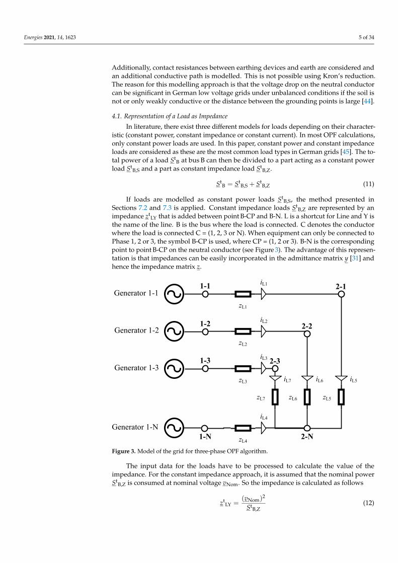
4.1. Representation of a Load as Impedance

In literature, there exist three different models for loads depending on their character-istic (constant power, constant impedance or constant current). In most OPF calculations,only constant power loads are used. In this paper, constant power and constant impedanceloads are considered as these are the most common load types in German grids [45]. The to-tal power of a load St

B at bus B can then be divided to a part acting as a constant powerload St

B,S and a part as constant impedance load StB,Z.

StB = St

B,S + StB,Z (11)

If loads are modelled as constant power loads StB,S, the method presented in

Sections 7.2 and 7.3 is applied. Constant impedance loads StB,Z are represented by an

impedance ztLY that is added between point B-CP and B-N. L is a shortcut for Line and Y is

the name of the line. B is the bus where the load is connected. C denotes the conductorwhere the load is connected C = (1, 2, 3 or N). When equipment can only be connected toPhase 1, 2 or 3, the symbol B-CP is used, where CP = (1, 2 or 3). B-N is the correspondingpoint to point B-CP on the neutral conductor (see Figure 3). The advantage of this represen-tation is that impedances can be easily incorporated in the admittance matrix y [31] andhence the impedance matrix z.

zL1

zL2

zL3

zL4

zL7 zL6 zL5

1-1

1-2

1-3 2-3

2-2

2-1

2-N1-N

Generator 1-1

Generator 1-2

Generator 1-3

Generator 1-N

iL4

iL2

iL3

iL5iL6iL7

iL1

Figure 3. Model of the grid for three-phase OPF algorithm.

The input data for the loads have to be processed to calculate the value of theimpedance. For the constant impedance approach, it is assumed that the nominal powerSt

B,Z is consumed at nominal voltage vNom. So the impedance is calculated as follows

ztLY =

(vNom)2

StB,Z

(12)

Energies 2021, 14, 1623 6 of 34

As the power StB,Z consumed by the load may change in each time step t, the impedance

ztLY is also time-dependent. The impedances calculated here to represent a load are part

of the calculation of the impedance matrix z (see Section 4.2). As ztLY is time-dependent,

the admittance matrix y is equally time-dependent. A corresponding label zt or yt is notused in this paper, for better clarity and as constant impedance loads are only an optionalmodelling approach.

4.2. The Impedance Matrix

The impedance matrix z is used to calculate the currents and power flows in the griddepending on the voltages. ~vt is a vector containing all voltages at time step t. A vectorwith currents flowing on all lines~itLine can be calculated as follows:

~itLine = z−1 · ~vt = y · ~vt (13)

The admittance matrix y is the inverse of the impedance matrix z. For the test gridshown in Figure 3, the impedance matrix z is a 7 × 8 matrix having the following form:

itL1itL2itL3itL4itL5itL6itL7

=

z11 z12 z13 z14 z15 z16 z17 z18z21 z22 z23 z24 z25 z26 z27 z28z31 z32 z33 z34 z35 z36 z37 z38z41 z42 z43 z44 z45 z46 z47 z48z51 z52 z53 z54 z55 z56 z57 z58z61 z62 z63 z64 z65 z66 z67 z68z71 z72 z73 z74 z75 z76 z77 z78

−1

·

vt1-1

vt2-1

vt1-2

vt2-2

vt1-3

vt2-3

vt1-N

vt2-N

(14)

The naming is in accordance to Figure 3. vtB-C refers to the complex voltage at

point B-C. In Equation (15), the current on Line 1 itL1 is calculated as an example forthe grid in Figure 3.

itL1 =1

zL1· vt

1,1 −1

zL1· vt

2,1 =vt

1,1 − vt2,1

zL1(15)

For the test grid shown in Figure 3, the impedance matrix z has the following entries:

itL1itL2itL3itL4itL5itL6itL7

=

zL1 −zL1 0 0 0 0 0 00 0 zL2 −zL2 0 0 0 00 0 0 0 zL3 −zL3 0 00 0 0 0 0 0 zL4 −zL40 zL5 0 0 0 0 0 −zL50 0 0 zL6 0 0 0 −zL60 0 0 0 0 zL7 0 −zL7

−1

·

vt1-1

vt2-1

vt1-2

vt2-2

vt1-3

vt2-3

vt1-N

vt2-N

(16)

In real low voltage grids, there are inductive and conductive couplings between thedifferent phases as seen in Figure 4. For a correct calculation, especially for unbalancedpower flows, these mutual impedances have to be considered [44].

Energies 2021, 14, 1623 7 of 34

zL1

zL2

zL3

zL4

zL7 zL6 zL5

1-1

1-2

1-3 2-3

2-2

2-1

2-N1-N

Generator 1-1

Generator 1-2

Generator 1-3

Generator 1-N

iL4

iL2

iL3

iL5iL6iL7

iL1

zL12

zL23

zL3N

zL13

zL2N

zL1N

Figure 4. Model of the grid for a three-phase OPF algorithm including mutual impedances.

Taking into account the mutual impedances leads to the following impedance matrix z:

z =

zL1 −zL1 zL12 −zL12 zL13 −zL13 zL1N −zL1NzL21 −zL21 zL2 −zL2 zL23 −zL23 zL2N −zL2NzL31 −zL31 zL32 −zL32 zL3 −zL3 zL3N −zL3NzLN1 −zLN1 zLN2 −zLN2 zLN3 −zLN3 z4 −z4

0 zL5 0 0 0 0 0 −zL50 0 0 zL6 0 0 0 −zL60 0 0 0 0 zL7 0 −zL7

(17)

Under normal circumstances, the impedances of a line zL1, zL2 and zL3 are equal.Therefore, zS is introduced as series impedance of the cable.

zS = zL1 = zL2 = zL3 = zL4 (18)

The mutual impedances are not the same as the distances between the differentconductors inside the cable are not the same. As can be seen in [44], the assumption ofsame impedances leads only to minor differences in the results, therefore the mean valueof the mutual impedance zM is used for all mutual impedances in this paper.

zM = zL12 = zL13 = zL1N = zL21 = zL23 = zL2N = zL31 = zL32 = zL3N (19)

= zLN1 = zLN2 = zLN3

Using the newly introduced variables zS and zM, the set of equations in Equation (17)can be simplified to Equation (20).

itL1itL2itL3itL4itL5itL6itL7

=

zS −zS zM −zM zM −zM zM −zMzM −zM zS −zS zM −zM zM −zMzM −zM zM −zM zS −zS zM −zMzM −zM zM −zM zM −zM zS −zS0 zL5 0 0 0 0 0 −zL50 0 0 zL6 0 0 0 −zL60 0 0 0 0 zL7 0 −zL7

−1

·

vt1-1

vt2-1

vt1-2

vt2-2

vt1-3

vt2-3

vt1-N

vt2-N

(20)

In Germany, there are several grounding points in a low voltage grid. Besides agrounding point at the low voltage side of the MV/LV transformer, there are additionalconnections to earth at each household as well as at cable distribution cabinets. Hence,an additional conductive path exists through earth. As shown in [44], neglecting this

Energies 2021, 14, 1623 8 of 34

conductive path leads to significant deviations. To model the conductive path throughearth, an approach presented in [44] is used. It consists of an imaginary point that representsthe earth. This point is named E in Figure 5.

All points in the low voltage grid being grounded are connected to this point directlyvia an earthing resistance. This earthing resistance consists of the contact resistance betweenearthing device and ground as well as the resistance of the ground. In Table 1, the values ofthe assumed earthing resistances according to [44] are shown.

Table 1. Earthing resistances from [44].

Equipment Earthing Resistance

Transformer 6 ΩHousehold 2 Ω

Cable distribution cabinet 2 Ω

zL1

zL2

zL3

zL4

zL7 zL6 zL5

1-1

1-2

1-3 2-3

2-2

2-1

2-N

1-N

Generator 1-1

Generator 1-2

Generator 1-3

Generator 1-N

iL4

iL2

iL3

iL5iL6iL7

iL1

zL12

zL23

zL3N

zL13

zL2N

zL1N

EzL8 zL9

iL8 iL9

Figure 5. Model of the grid for a three-phase OPF algorithm including mutual impedances andearthing impedances.

As the points 1-1, 1-2, 1-3 and 1-N in Figure 4 model the low voltage side of a MV/LVtransformer and the points 2-1, 2-2, 2-3 and 2-N for example a load in a household, the re-sulting grid model including grounding points can be seen in Figure 5. The correspondingimpedance matrix z is then a 9 × 9 matrix as shown in Equation (21).

itL1itL2itL3itL4itL5itL6itL7itL8itL9

=

zS −zS zM −zM zM −zM zM −zM 0zM −zM zS −zS zM −zM zM −zM 0zM −zM zM −zM zS −zS zM −zM 0zM −zM zM −zM zM −zM zS −zS 00 zL5 0 0 0 0 0 −zL5 00 0 0 zL6 0 0 0 −zL6 00 0 0 0 0 zL7 0 −zL7 00 0 0 0 0 0 zL8 0 −zL80 0 0 0 0 0 0 zL9 −zL9

−1

·

vt1-1

vt2-1

vt1-2

vt2-2

vt1-3

vt2-3

vt1-N

vt2-N

vtE

(21)

Energies 2021, 14, 1623 9 of 34

4.3. The Nodal Impedance Matrix

The nodal impedance matrix zNodal is calculated using z and is used to calculate thesum of the currents that are flowing from a point B-C to other points. ~itBus is a vectorcontaining all these currents while itB-C refers to the sum of the currents at point B-C.

~itBus = zNodal−1 · ~vt (22)

Consequently, itB-C can be calculated using the currents given in Equation (21).

it1-1it2-1it1-2it2-2it1-3it2-3it1-Nit2-NitE

=

itL1−itL1 + itL5

itL2−itL2 + itL6

itL3−itL3 + itL7itL4 + itL8

−itL4 − itL5 − itL6 − itL7 + itL9−itL8 − itL9

(23)

Assuming, a grid structure like in Figure 5, zNodal is a 9x9 matrix.

zNodal =

zNodal,11 zNodal,12 zNodal,13 zNodal,14 zNodal,15 zNodal,16 zNodal,17 zNodal,18 zNodal,19zNodal,21 zNodal,22 zNodal,23 zNodal,24 zNodal,25 zNodal,26 zNodal,27 zNodal,28 zNodal,29zNodal,31 zNodal,32 zNodal,33 zNodal,34 zNodal,35 zNodal,36 zNodal,37 zNodal,38 zNodal,39zNodal,41 zNodal,42 zNodal,43 zNodal,44 zNodal,45 zNodal,46 zNodal,47 zNodal,48 zNodal,49zNodal,51 zNodal,52 zNodal,53 zNodal,54 zNodal,55 zNodal,56 zNodal,57 zNodal,58 zNodal,59zNodal,61 zNodal,62 zNodal,63 zNodal,64 zNodal,65 zNodal,66 zNodal,67 zNodal,68 zNodal,69zNodal,71 zNodal,72 zNodal,73 zNodal,74 zNodal,75 zNodal,76 zNodal,77 zNodal,78 zNodal,79zNodal,81 zNodal,82 zNodal,83 zNodal,84 zNodal,85 zNodal,86 zNodal,87 zNodal,88 zNodal,89zNodal,91 zNodal,92 zNodal,93 zNodal,94 zNodal,95 zNodal,96 zNodal,97 zNodal,98 zNodal,99

(24)

=

zS −zS zM −zM zM −zM zM −zM 0−zS zS + zL5 −zM zM −zM zM −zM zM − zL5 0zM −zM zS −zS zM −zM zM −zM 0−zM zM −zS zS + zL6 −zM zM −zM zM − zL6 0zM −zM zM −zM zS −zS zM −zM 0−zM zM −zM zM −zS zS + zL7 −zM zM − zL7 0zM −zM zM −zM zM −zM zS + zL8 −zS −zL8−zM zM − zL5 −zM zM − zL6 −zM zM − zL7 −zS zNodal,88 −zL9

0 0 0 0 0 0 −zL8 −zL9 zL8 + zL9

(25)

zNodal,88 = zL5 + zL6 + zL7 + zS + zL9 (26)

Each impedance as well as each admittance can be divided to a real part and animaginary part. In Equation (27), the terms used in this publication for each part of theadmittance are introduced. Subsequently, the real and imaginary part will be often regardedseparately, because the constraints (see Section 7) have to be formulated consisting only ofreal numbers.

y = a + j · b (27)

5. Optimization Variables

All optimization variables for one time step are part of the vector x. The numberof optimization variables are determined in the following section for an exemplary gridcontaining only two buses (see Figure 5) for a single time step.

Energies 2021, 14, 1623 10 of 34

At first, vector x contains the voltages on all points B-C, where B denotes the bus andC the corresponding phase or neutral. The complex voltage is divided to two parts, the realand imaginary part which are denoted as follows.

vtB-C = et

B-C + j · f tB-C (28)

For the exemplary grid, these are 16 variables (2 buses · 4 voltages per bus · 2 partsper voltage). Furthermore, vector x contains the real and imaginary part of the voltage atearth (point E in Figure 5).

Additionally, the active power PtG,B-C as well as the reactive power Qt

G,B-C of allgenerators are part of the vector x. G is a shortcut for generator and B-C refers to thepoint of connection of the generator. As there are four generators, there are in total8 optimization variables.

To include battery storage system, the energy capacity EtS,B of the system is another

variable in the vector x. S is here a shortcut for storage and B is the bus where the storage isconnected. Besides, the active charging Pt

S,C,B-CP, active discharging power PtS,D,B-CP and

reactive power QtS,B-CP needs to be considered. Depending on the design of the battery

system, it can be connected to different phases CP at the same bus B. Including one batterysystem that is connected to all three phases leads to 10 optimization variables.

In total, optimization vector x contains 26 variables without and 36 variables includingthe battery system. In comparison, the optimization vector x would contain 6 variableswithout and 10 variables including the battery system for a traditional balanced powerflow formulation (see Figure 1).

6. Cost Function

For the cost function, costs are taken into account using cost factors c. These factors aremultiplied with a corresponding power and the duration of one time step. In Equation (29),an example is shown where the energy of the generators is priced.

Ft = (c1PtG,1-1 + c2Pt

G,1-2 + c3PtG,1-3 + c4Pt

G,1-N) · ∆t (29)

The cost function in Equation (29) is used in the following simulations. The costfactors of the generator connected to one of the three phases are set to the same value. Thisvalue has to be higher than zero to represent the generation costs, so that no unnecessaryenergy consumption in the low voltage feeder is encouraged. In this paper, it is set to 28 torepresent average energy consumption costs in Germany of 28 ct/kWh.

c1 = c2 = c3 = 28 (30)

On the neutral conductor, the current is only flowing back so that no extra costsare assumed.

c4 = 0 (31)

Depending on the optimization goal, the power flow over specific lines or otherequipment like a battery storage can be considered additionally.

7. Constraints for the Formulation of the Optimization Problem

In this chapter, the equality and inequality constraints are described. The solverrequires the first and second order derivatives of the constraints to solve the optimizationproblem. For constraints that have already been introduced in literature (e.g., the powerflow constraint in Section 7.2), these derivatives are neither given nor mentioned in thissection. Only the constraints are explained to the reader.

Energies 2021, 14, 1623 11 of 34

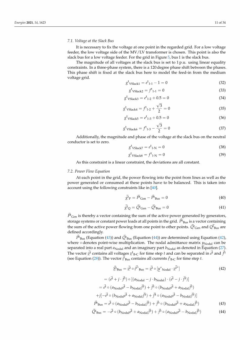
7.1. Voltage at the Slack Bus

It is necessary to fix the voltage at one point in the regarded grid. For a low voltagefeeder, the low voltage side of the MV/LV transformer is chosen. This point is also theslack bus for a low voltage feeder. For the grid in Figure 5, bus 1 is the slack bus.

The magnitude of all voltages at the slack bus is set to 1 p.u. using linear equalityconstraints. In a three-phase system, there is a 120 degree phase shift between the phases.This phase shift is fixed at the slack bus here to model the feed-in from the mediumvoltage grid.

gtVSlack1 = et

1-1 − 1 = 0 (32)

gtVSlack2 = f t

1-1 = 0 (33)

gtVSlack3 = et

1-2 + 0.5 = 0 (34)

gtVSlack4 = f t

1-2 +

√3

2= 0 (35)

gtVSlack5 = et

1-3 + 0.5 = 0 (36)

gtVSlack6 = f t

1-3 −√

32

= 0 (37)

Additionally, the magnitude and phase of the voltage at the slack bus on the neutralconductor is set to zero.

gtVSlack7 = et

1-N = 0 (38)

gtVSlack8 = f t

1-N = 0 (39)

As this constraint is a linear constraint, the deviations are all constant.

7.2. Power Flow Equation

At each point in the grid, the power flowing into the point from lines as well as thepower generated or consumed at these points have to be balanced. This is taken intoaccount using the following constraints like in [40].

~gtP = ~Pt

Gen − ~PtBus = 0 (40)

~gtQ = ~Qt

Gen − ~QtBus = 0 (41)

~PtGen is thereby a vector containing the sum of the active power generated by generators,

storage systems or constant power loads at all points in the grid. ~PtBus is a vector containing

the sum of the active power flowing from one point to other points. ~QtGen and Q~tBus are

defined accordingly.~Pt

Bus (Equation (43)) and ~QtBus (Equation (44)) are determined using Equation (42),

where denotes point-wise multiplication. The nodal admittance matrix yNodal can beseparated into a real part aNodal and an imaginary part bNodal as denoted in Equation (27).The vector ~vt contains all voltages vt

B-C for time step t and can be separated in ~et and ~f t

(see Equation (28)). The vector itBus contains all currents itB-C for time step t.

~StBus = ~vt ~it∗Bus = ~vt [y∗Nodal · ~vt∗] (42)

= (~et + j · ~f t) [(aNodal − j · bNodal) · (~et − j · ~f t)]

= ~et (aNodal~et − bNodal

~f t) + ~f t (bNodal~et + aNodal

~f t)

+j[−~et (bNodal~et + aNodal

~f t) + ~f t (aNodal~et − bNodal

~f t)]

~PtBus = ~et (aNodal

~et − bNodal~f t) + ~f t (bNodal

~et + aNodal~f t) (43)

~QtBus = −~et (bNodal

~et + aNodal~f t) + ~f t (aNodal

~et − bNodal~f t) (44)

Energies 2021, 14, 1623 12 of 34

7.3. Current Equation

Besides a formulation like in Equations (40) and (41) using power flows, the currentsflowing into each point can also be used to formulate an equality constraint. This wasintroduced in TOPF in [14,17].

~itBus = yNodal · ~vt = (aNodal + j · bNodal)(~et + j · ~f t) (45)

= aNodal ·~et − bNodal · ~f t + j(bNodal ·~et + aNodal · ~f t)

The disadvantage of this approach is that power generated or consumed at the con-cerned bus (see ~Pt

Gen and ~QtGen in Equations (40) and (41)) can not be considered. Hence,

current based equality constraints are only used on points where ~PtGen and ~Qt

Gen are zero.On the neutral conductor, the power flow is significantly lower than on the other phases.Assuming similar absolute errors in the fulfillment of power flow based equality constraints(see Section 7.2), the relative error is significantly higher on the neutral conductor. Hence,it is beneficial to use current equations on the neutral conductor as currents are in a similarorder as on the other phases for unbalanced power flows. Besides a higher accuracy andbetter conditioned matrices, another advantage is that linear constraints are used instead ofnonlinear constraints. The above mentioned disadvantage of this approach is not essentialas no power is consumed or generated on the neutral conductor. The only exception isthe slack bus due to the generator. In this publication, the current equation instead of thepower flow equation is used for all points on the neutral conductor except the slack bus.

For a formulation as a constraints, Equation (45) has to be divided into two parts: Oneconstraint contains the real part and the second the imaginary part of Equation (45). Therelated constraints are formulated as follows:

~gti,Real = aNodal ·~et − bNodal · ~f t = 0 (46)

~gti,Imag = bNodal ·~et + aNodal · ~f t = 0 (47)

When generators, storage systems or constant power loads are part of the regardedgrid, the total generated power at point B-CP Pt

G,B-CP and QtG,B-CP is considered in

Equations (40) and (41). As the power flow on the neutral conductor is considered inthis paper, the negative value of the current being fed into the grid at point B-CP has tobe fed-in at point B-N, where point B-N is the corresponding point to B-CP on the neutralconductor of the same bus. This is ensured by expanding the current equation as explainedin the following paragraphs.

The current itG,B-CP that is inserted at point B-CP can be calculated as follows

itG,B-CP =

(St

Bus,B-CP

vtB-CP

)* =

(Pt

Bus,B-CP − jQtBus,B-CP

etB-CP − j f t

B-CP

)(et

B-CP + j f tB-CP

etB-CP + j f t

B-CP

)(48)

=Pt

Bus,B-CPetB-CP + Qt

Bus,B-CP f tB-CP + j(Pt

Bus,B-CP f tB-CP −Qt

Bus,B-CPetB-CP)

(etB-CP)2 + ( f t

B-CP)2

itG,B-CP,Real =Pt

Bus,B-CPetB-CP + Qt

Bus,B-CP f tB-CP

(etB-CP)2 + ( f t

B-CP)2 (49)

itG,B-CP,Imag =Pt

Bus,B-CP f tB-CP −Qt

Bus,B-CPetB-CP

(etB-CP)2 + ( f t

B-CP)2 (50)

The vectors~itG,Real and~itG,Imag contain the real and imaginary part of the current thatis inserted at all points.

~itG,Real =~Pt

Bus ~et + ~QtBus ~f t

(~et)2 + (~f t)2(51)

Energies 2021, 14, 1623 13 of 34

~itG,Imag =~Pt

Bus ~f t − ~QtBus ~et

(~et)2 + (~f t)2(52)

The current equations as defined in Equations (46) and (47) are adapted as shownin Equations (53) and (54). Please note that fraction line means pointwise division inEquations (51)–(54).

~gti,Real = aNodal ·~et − bNodal · ~f t − (−S · itG,B-CP,Imag) (53)

= aNodal ·~et − bNodal · ~f t + S ·~Pt

Bus ~et + ~QtBus ~f t

(~et)2 + (~f t)2= 0

~gti,Imag = bNodal ·~et + aNodal · ~f t − (−S ·~itG,Imag) (54)

= bNodal ·~et + aNodal · ~f t + S ·~Pt

Bus ~f t − ~QtBus ~et

(~et)2 + (~f t)2= 0

The negative value of the current which is fed into the grid at point B-CP has to befed-in at point B-N, where point B-N is the corresponding point to B-CP on the same bus onthe neutral conductor. The allocation of the current which is fed into the grid at point B-CPto the corresponding current on point B-N on the neutral conductor is done by matrix S.

The first order derivatives of itG,B-CP,Real and itG,B-CP,Imag are given inEquations (55)–(62).

∂itG,B-CP,Real

∂PtBus,B-CP

=et

B-CP

(etB-CP)2 + ( f t

B-CP)2 (55)

∂itG,B-CP,Real

∂QtBus,B-CP

=f t

B-CP

(etB-CP)2 + ( f t

B-CP)2 (56)

∂itG,B-CP,Real

∂etB-CP

=Pt

Bus,B-CP((etB-CP)

2 + ( f tB-CP)

2)− (PtBus,B-CPet

B-CP + QtBus,B-CP f t

B-CP)2etB-CP

((etB-CP)2 + ( f t

B-CP)2)2 (57)

=−Pt

Bus,B-CP(etB-CP)

2 + PtBus,B-CP( f t

B-CP)2 − 2Qt

Bus,B-CP f tB-CPet

B-CP

((etB-CP)2 + ( f t

B-CP)2)2

∂itG,B-CP,Real

∂ f tB-CP

=Qt

Bus,B-CP((etB-CP)

2 + ( f tB-CP)

2)− (PtBus,B-CPet

B-CP + QtBus,B-CP f t

B-CP)2 f tB-CP

((etB-CP)2 + ( f t

B-CP)2)2 (58)

=Qt

Bus,B-CP(etB-CP)

2 −QtBus,B-CP( f t

B-CP)2 − 2Pt

Bus,B-CP f tB-CPet

B-CP

((etB-CP)2 + ( f t

B-CP)2)2

∂itG,B-CP,Imag

∂PtBus,B-CP

=f t

B-CP

(etB-CP)2 + ( f t

B-CP)2 (59)

∂itG,B-CP,Imag

∂QtBus,B-CP

=−et

B-CP

(etB-CP)2 + ( f t

B-CP)2 (60)

∂itG,B-CP,Imag

∂etB-CP

=−Qt

Bus,B-CP((etB-CP)

2 + ( f tB-CP)

2)− (PtBus,B-CP f t

B-CP −QtBus,B-CPet

B-CP)2etB-CP

((etB-CP)2 + ( f t

B-CP)2)2 (61)

=−Qt

Bus,B-CP( f tB-CP)

2 + QtBus,B-CP(et

B-CP)2 − 2Pt

Bus,B-CP f tB-CPet

B-CP

((etB-CP)2 + ( f t

B-CP)2)2

∂itG,B-CP,Imag

∂ f tB-CP

=Pt

Bus,B-CP((etB-CP)

2 + ( f tB-CP)

2)− (PtBus,B-CP f t

B-CP −QtBus,B-CPet

B-CP)2 f tB-CP

((etB-CP)2 + ( f t

B-CP)2)2 (62)

=−Pt

Bus,B-CP( f tB-CP)

2 + PtBus,B-CP(et

B-CP)2 + 2Qt

Bus,B-CP f tB-CPet

B-CP

((etB-CP)2 + ( f t

B-CP)2)2

Energies 2021, 14, 1623 14 of 34

All non-zero second derivatives are given from Equations (63)–(86).

∂2itG,B-CP,Real

∂PtBus,B-CP∂et

B-CP=

(etB-CP)

2 + ( f tB-CP)

2 − etB-CP · 2et

B-CP

((etB-CP)2 + ( f t

B-CP)2)2 (63)

=−(et

B-CP)2 + ( f t

B-CP)2

((etB-CP)2 + ( f t

B-CP)2)2

∂2itG,B-CP,Real

∂PtBus,B-CP∂ f t

B-CP=

−2etB-CP · f t

B-CP

((etB-CP)2 + ( f t

B-CP)2)2 (64)

∂2itG,B-CP,Real

∂QtBus,B-CP∂et

B-CP=

−2 f tB-CP · et

B-CP

((etB-CP)2 + ( f t

B-CP)2)2 (65)

∂2itG,B-CP,Real

∂QtBus,B-CP∂ f t

B-CP=

(etB-CP)

2 + ( f tB-CP)

2 − f tB-CP · 2 f t

B-CP

((etB-CP)2 + ( f t

B-CP)2)2 (66)

=(et

B-CP)2 − ( f t

B-CP)2

((etB-CP)2 + ( f t

B-CP)2)2

∂2itG,B-CP,Real

∂etB-CP

2 =(−2Pt

Bus,B-CPetB-CP − 2Qt

Bus,B-CP f tB-CP) · ((et

B-CP)2 + ( f t

B-CP)2)

((etB-CP)2 + ( f t

B-CP)2)3 (67)

− (−PtBus,B-CP(et

B-CP)2 + Pt

Bus,B-CP( f tB-CP)

2 − 2QtBus,B-CP f t

B-CPetB-CP) · 4et

B-CP

((etB-CP)2 + ( f t

B-CP)2)3

∂2itG,B-CP,Real

∂etB-CP∂ f t

B-CP=

(2PtBus,B-CP f t

B-CP − 2QtBus,B-CPet

B-CP) · ((etB-CP)

2 + ( f tB-CP)

2)

((etB-CP)2 + ( f t

B-CP)2)3 (68)

− (−PtBus,B-CP(et

B-CP)2 + Pt

Bus,B-CP( f tB-CP)

2 − 2QtBus,B-CP f t

B-CPetB-CP) · 4 f t

B-CP

((etB-CP)2 + ( f t

B-CP)2)3

∂2itG,B-CP,Real

∂etB-CP∂Pt

Bus,B-CP=−(et

B-CP)2 + ( f t

B-CP)2

((etB-CP)2 + ( f t

B-CP)2)2 (69)

∂2itG,B-CP,Real

∂etB-CP∂Qt

Bus,B-CP=

−2etB-CP f t

B-CP

((etB-CP)2 + ( f t

B-CP)2)2 (70)

∂2itG,B-CP,Real

∂ f tB-CP∂et

B-CP=

(+2QtBus,B-CPet

B-CP − 2PtBus,B-CP f t

B-CP)((etB-CP)

2 + ( f tB-CP)

2)

((etB-CP)2 + ( f t

B-CP)2)3 (71)

− (+QtBus,B-CP(et

B-CP)2 −Qt

Bus,B-CP( f tB-CP)

2 − 2PtBus,B-CP f t

B-CPetB-CP) · 4et

B-CP

((etB-CP)2 + ( f t

B-CP)2)3

∂2itG,B-CP,Real

∂ f tB-CP

2 =(−2Qt

Bus,B-CP f tB-CP − 2Pt

Bus,B-CPetB-CP)((et

B-CP)2 + ( f t

B-CP)2)

((etB-CP)2 + ( f t

B-CP)2)3 (72)

− (+QtBus,B-CP(et

B-CP)2 −Qt

Bus,B-CP( f tB-CP)

2 − 2PtBus,B-CP f t

B-CPetB-CP) · 4 f t

B-CP

((etB-CP)2 + ( f t

B-CP)2)3

∂2itG,B-CP,Real

∂ f tB-CP∂Pt

Bus,B-CP=

−2 f tB-CPet

B-CP

((etB-CP)2 + ( f t

B-CP)2)2 (73)

∂2itG,B-CP,Real

∂ f tB-CP∂Qt

Bus,B-CP=

+(etB-CP)

2 − ( f tB-CP)

2

((etB-CP)2 + ( f t

B-CP)2)2 (74)

∂2itG,B-CP,Imag

∂PtBus,B-CP∂et =

−2 f tB-CP · et

B-CP

((etB-CP)2 + ( f t

B-CP)2)2 (75)

∂2itG,B-CP,Imag

∂PtBus,B-CP∂ f t

Bus,B-CP=

((etB-CP)

2 + ( f tB-CP)

2)− f tB-CP2 f t

B-CP

((etB-CP)2 + ( f t

B-CP)2)2 (76)

Energies 2021, 14, 1623 15 of 34

=(et

B-CP)2 − ( f t

B-CP)2

((etB-CP)2 + ( f t

B-CP)2)2

∂2itG,B-CP,Imag

∂QtBus,B-CP∂et

B-CP=−((et

B-CP)2 + ( f t

B-CP)2) + et

B-CP2etB-CP

((etB-CP)2 + ( f t

B-CP)2)2 (77)

=(et

B-CP)2 − ( f t

B-CP)2

((etB-CP)2 + ( f t

B-CP)2)2

∂2itG,B-CP,Imag

∂QtBus,B-CP∂ f t

B-CP=

2etB-CP f t

B-CP

((etB-CP)2 + ( f t

B-CP)2)2 (78)

∂2itG,B-CP,Imag

∂etB-CP

2 =(2Qt

Bus,B-CPetB-CP − 2Pt

Bus,B-CP f tB-CP)((et

B-CP)2 + ( f t

B-CP)2)

((etB-CP)2 + ( f t

B-CP)2)3 (79)

− (−QtBus,B-CP( f t

B-CP)2 + Qt

Bus,B-CP(etB-CP)

2 − 2PtBus,B-CP f t

B-CPetB-CP) · 4et

B-CP

((etB-CP)2 + ( f t

B-CP)2)3

∂2itG,B-CP,Imag

∂etB-CP∂ f t

B-CP=

(−2QtBus,B-CP f t

B-CP − 2PtBus,B-CPet

B-CP)((etB-CP)

2 + ( f tB-CP)

2)

((etB-CP)2 + ( f t

B-CP)2)3 (80)

− (−QtBus,B-CP( f t

B-CP)2 + Qt

Bus,B-CP(etB-CP)

2 − 2PtBus,B-CP f t

B-CPetB-CP) · 4 f t

B-CP

((etB-CP)2 + ( f t

B-CP)2)3

∂2itG,B-CP,Imag

∂etB-CP∂Pt

Bus,B-CP=

−2 f tB-CPet

B-CP

((etB-CP)2 + ( f t

B-CP)2)2 (81)

∂2itG,B-CP,Imag

∂etB-CP∂Qt

Bus,B-CP=−( f t

B-CP)2 + (et

B-CP)2

((etB-CP)2 + ( f t

B-CP)2)2 (82)

∂2itG,B-CP,Imag

∂ f tB-CP∂et

B-CP=

(2PtBus,B-CPet

B-CP + 2QtBus,B-CP f t

B-CP)((etB-CP)

2 + ( f tB-CP)

2)

((etB-CP)2 + ( f t

B-CP)2)3 (83)

− (−PtBus,B-CP( f t

B-CP)2 + Pt

Bus,B-CP(etB-CP)

2 + 2QtBus,B-CP f t

B-CPetB-CP) · 4et

B-CP

((etB-CP)2 + ( f t

B-CP)2)3

∂2itG,B-CP,Imag

∂ f tB-CP

2 =(−2Pt

Bus,B-CP f tB-CP + 2Qt

Bus,B-CPetB-CP)((et

B-CP)2 + ( f t

B-CP)2)

((etB-CP)2 + ( f t

B-CP)2)3 (84)

− (−PtBus,B-CP( f t

B-CP)2 + Pt

Bus,B-CP(etB-CP)

2 + 2QtBus,B-CP f t

B-CPetB-CP) · 4 f t

B-CP

((etB-CP)2 + ( f t

B-CP)2)3

∂2itG,B-CP,Imag

∂ f tB-CP∂Pt

Bus,B-CP=−( f t

B-CP)2 + (et

B-CP)2

((etB-CP)2 + ( f t

B-CP)2)2 (85)

∂2itG,B-CP,Imag

∂ f tB-CP∂Qt

Bus,B-CP=

2 f tB-CPet

B-CP

((etB-CP)2 + ( f t

B-CP)2)2 (86)

7.4. Limits for the Voltages in the Grid

For the voltage at each point, upper as well as lower voltage limits are defined (e.g.,in [46] for Europe). For the three-phase algorithm, it is important to mention that the validvoltage at consumer level is the difference between phase voltage and neutral conductorvoltage. Hence, for each point on Phase 1, 2 or 3, the difference between phase andneutral conductor voltage is constrained between a minimum allowed voltage vMin and amaximum allowed voltage vMax.

htVMax = (et

B-CP − etB-N)

2 + ( f tB-CP − f t

B-N)2 − (vMax)

2 ≤ 0 (87)

htVMin = −(et

B-CP − etB-N)

2 − ( f tB-CP − f t

B-N)2 + (vMin)

2 ≤ 0 (88)

Energies 2021, 14, 1623 16 of 34

All non-zero derivatives are shown in Equations (89)–(96).

∂htVMax

∂etB-CP

= 2(etB-CP − et

B-N) (89)

∂htVMax

∂etB-N

= −2(etB-CP − et

B-N) (90)

∂htVMax

∂ f tB-CP

= 2( f tB-CP − f t

B-N) (91)

∂htVMax

∂ f tB-N

= −2( f tB-CP − f t

B-N) (92)

∂htVMin

∂etB-CP

= −2(etB-CP − et

B-N) (93)

∂htVMin

∂etB-N

= 2(etB-CP − et

B-N) (94)

∂htVMin

∂ f tB-CP

= −2( f tB-CP − f t

B-N) (95)

∂htVMin

∂ f tB-N

= 2( f tB-CP − f t

B-N) (96)

All second derivatives of these constraints are constant. All second derivatives notgiven in Equations (97) and (98) are zero.

∂2htVMax

∂etB-CP∂et

B-CP=

∂2htVMax

∂etB-N∂et

B-N=

∂2htVMax

∂ f tB-CP∂ f t

B-CP=

∂2htVMax

∂ f tB-N∂ f t

B-N(97)

=∂2ht

VMin

∂etB-CP∂et

B-N=

∂2htVMin

∂etB-N∂et

B-CP=

∂2htVMin

∂ f tB-CP∂ f t

B-N=

∂2htVMin

∂ f tB-N∂ f t

B-CP= 2

∂2htVMax

∂etB-CP∂et

B-N=

∂2htVMax

∂etB-N∂et

B-CP=

∂2htVMax

∂ f tB-CP∂ f t

B-N=

∂2htVMax

∂ f tB-N∂ f t

B-CP(98)

=∂2ht

VMin

∂etB-CP∂et

B-CP=

∂2htVMin

∂etB-N∂et

B-N=

∂2htVMin

∂ f tB-CP∂ f t

B-CP=

∂2htVMin

∂ f tB-N∂ f t

B-N= −2

7.5. Limit for Voltage Unbalance

The allowed voltage unbalance can be limited in low voltage grids. For examplein Europe, the maximum voltage unbalance at consumer level is set to 2% according toEN 50160:2010/A1:2015 [46]. The voltage unbalance vt

Unb,B at bus B is defined in [46]as the ratio between the negative sequence voltage vt

Neg,B and the positive sequencevoltage vt

Pos,B.

vtUnb,B =

|vtNeg,B||vt

Pos,B|(99)

In [21], the voltage unbalance is also taken into account for storage operation. In con-trast to this paper, [21] uses approximations for the constraints and derivatives to be ableto solve the optimization problem. Here, the constraint and all derivatives are calculatedexactly as can be seen in the upcoming equations for higher accuracy.

In the following equations, d is used for reasons of simplification.

d = −12+ j√

32

(100)

Energies 2021, 14, 1623 17 of 34

For a proper formulation of constraints, vtNeg,B and vt

Pos,B have to be formulatedusing optimization variables. The negative sequence voltage vt

Neg,B at bus B is defined asin Equation (101).

vtNeg,B =

13((vt

B-1 − vtB-N) + d2(vt

B-2 − vtB-N) + d(vt

B-3 − vtB-N)) (101)

=13(((et

B-1 + j · f tB-1)− (et

B-N + j · f tB-N))

+(−12− j√

32

)((etB-2 + j · f t

B-2)− (etB-N + j · f t

B-N))

+(−12+ j√

32

)((etB-3 + j · f t

B-3)− (etB-N + j · f t

B-N)))

etNeg,B and f t

Neg,B are introduced as real and imaginary part of vtNeg,B.

etNeg,B =

13· (et

B-1 −12

etB-2 −

12

etB-3 +

√3

2f t

B-2 −√

32

f tB-3) (102)

f tNeg,B =

13· (−√

32· et

B-2 +

√3

2et

B-3 + f tB-1 −

12

f tB-2 −

12

f tB-3) (103)

Likewise, in Equation (104), the positive sequence voltage vtPos,B is defined and then

splitted to real and imaginary parts in Equations (105) and (106).

vtPos,B =

13((vt

B-1 − vtB-N) + d(vt

B-2 − vtB-N) + d2(vt

X,3 − vtB-N)) (104)

=13· (et

B-1 −12

etB-2 −

12

etB-3 −

√3

2f t

B-2 +

√3

2f t

B-3

+j · (√

32· et

B-2 −√

32

etB-3 + f t

B-1 −12

f tB-2 −

12

f tB-3))

etPos,B =

13(et

B-1 −12

etB-2 −

12

etB-3 −

√3

2f t

B-2 +

√3

2f t

B-3) (105)

f tPos,B =

13· (√

32· et

B-2 −√

32

etB-3 + f t

B-1 −12

f tB-2 −

12

f tB-3) (106)

The constraint for voltage unbalance at bus B of the grid is then defined as the follow-ing inequality constraint:

htUnb,B =

|vtNeg,B|2

|vtPos,B|2

− vUnb,Max2 =

(etNeg,B)

2 + ( f tNeg,B)

2

(etPos,B)2 + ( f t

Pos,B)2 − vUnb,Max2 ≤ 0 (107)

vUnb,Max defines the applied limit for the voltage unbalance. For the optimization algorithm,the first and second derivatives of the constraint in Equation (107) with respect to allvariables in the vector x have to be derived. As Equation (107) consists only of realand imaginary parts of voltages, all derivatives with respect to other quantities are zero.In Equation (108), the first order derivative of the voltage unbalance constraint ht

Unb,B isgiven with respect to k. k is any real part et

B-C or imaginary part f tB-C of a voltage.

∂htUnb,B

∂k=

∂

∂k(et

Neg,B)2 + ( f t

Neg,B)2

(etPos,B)2 + ( f t

Pos,B)2 (108)

=(2et

Neg,B ·∂et

Neg,B∂k + 2 f t

Neg,B ·∂ f t

Neg,B∂k )((et

Pos,B)2 + ( f t

Pos,B)2)

((etPos,B)2 + ( f t

Pos,B)2)2

Energies 2021, 14, 1623 18 of 34

−(2et

Pos,B ·∂et

Pos,B∂k + 2 f t

Pos,B ·∂ f t

Pos,B∂k )((et

Neg,B)2 + ( f t

Neg,B)2)

((etPos,B)2 + ( f t

Pos,B)2)2

=2(et

Neg,B ·∂et

Neg,B∂k + f t

Neg,B ·∂ f t

Neg,B∂k )

((etPos,B)2 + ( f t

Pos,B)2)

−2(et

Pos,B ·∂et

Pos,B∂k + f t

Pos,B ·∂ f t

Pos,B∂k )((et

Neg,B)2 + ( f t

Neg,B)2)

((etPos,B)2 + ( f t

Pos,B)2)2

The second derivatives are given in the following equations. Here, htUnb,B is derived

with respect to a real or imaginary part of a voltage k and with respect to a real or imaginarypart of a voltage l.

∂2htUnb,B

∂k∂l=

(2 ·∂et

Neg,B∂k

∂etNeg,B∂l + 2 ·

∂ f tNeg,B∂k

∂ f tNeg,B∂l )((et

Pos,B)2 + ( f t

Pos,B)2)((et

Pos,B)2 + ( f t

Pos,B)2)2

((etPos,B)2 + ( f t

Pos,B)2)4 (109)

+(2et

Neg,B ·∂et

Neg,B∂k + 2 f t

Neg,B ·∂ f t

Neg,B∂k )(2et

Pos,B ·∂et

Pos,B∂l + 2 f t

Pos,B ·∂ f t

Pos,B∂l )((et

Pos,B)2 + ( f t

Pos,B)2)2

((etPos,B)2 + ( f t

Pos,B)2)4

−(2et

Neg,B ·∂et

Neg,B∂k + 2 f t

Neg,B ·∂ f t

Neg,B∂k ) · 2((et

Pos,B)2 + ( f t

Pos,B)2)2(2et

Pos,B ·∂et

Pos,B∂l + 2 f t

Pos,B ·∂ f t

Pos,B∂l )

((etPos,B)2 + ( f t

Pos,B)2)4

−(2 · ∂et

Pos,B∂k

∂etPos,B∂l + 2 · ∂ f t

Pos,B∂k

∂ f tPos,B∂l )((et

Neg,B)2 + ( f t

Neg,B)2)((et

Pos,B)2 + ( f t

Pos,B)2)2

((etPos,B)2 + ( f t

Pos,B)2)4

−(2et

Pos,B ·∂et

Pos,B∂k + 2 f t

Pos,B ·∂ f t

Pos,B∂k )(2et

Neg,B ·∂et

Neg,B∂l + 2 f t

Neg,B ·∂ f t

Neg,B∂l )((et

Pos,B)2 + ( f t

Pos,B)2)2

((etPos,B)2 + ( f t

Pos,B)2)4

+(2et

Pos,B ·∂et

Pos,B∂k + 2 f t

Pos,B ·∂ f t

Pos,B∂k )((et

Neg,B)2 + ( f t

Neg,B)2) · 2((et

Pos,B)2 + ( f t

Pos,B)2)

((etPos,B)2 + ( f t

Pos,B)2)4

·(2et

Pos,B ·∂et

Pos,B∂l + 2 f t

Pos,B ·∂ f t

Pos,B∂l )

1

=2(

∂etNeg,B∂k

∂etNeg,B∂l +

∂ f tNeg,B∂k

∂ f tNeg,B∂l )

(etPos,B)2 + ( f t

Pos,B)2

−4(et

Neg,B ·∂et

Neg,B∂k + f t

Neg,B ·∂ f t

Neg,B∂k )(et

Pos,B ·∂et

Pos,B∂l + f t

Pos,B ·∂ f t

Pos,B∂l )

((etPos,B)2 + ( f t

Pos,B)2)2

−2(

∂etPos,B∂k

∂etPos,B∂l +

∂ f tPos,B∂k

∂ f tPos,B∂l )((et

Neg,B)2 + ( f t

Neg,B)2)

((etPos,B)2 + ( f t

Pos,B)2)2

−4(et

Pos,B ·∂et

Pos,B∂k + f t

Pos,B ·∂ f t

Pos,B∂k )(et

Neg,B ·∂et

Neg,B∂l + f t

Neg,B ·∂ f t

Neg,B∂l )

((etPos,B)2 + ( f t

Pos,B)2)2

+8(et

Pos,B ·∂et

Pos,B∂k + f t

Pos,B ·∂ f t

Pos,B∂k )((et

Neg,B)2 + ( f t

Neg,B)2)(et

Pos,B ·∂et

Pos,B∂l + f t

Pos,B ·∂ f t

Pos,B∂l )

((etPos,B)2 + ( f t

Pos,B)2)3

Energies 2021, 14, 1623 19 of 34

The equations for first and second derivatives of the voltage unbalance constraintht

Unb,B, given in Equations (108) and (109), still contain further derivatives. These are givenin Equations (110) to (129). All derivatives not mentioned here are zero.

∂etNeg,B

∂etB-1

=13· 1 =

13

(110)

∂etNeg,B

∂etB-2

=13· −1

2= −1

6(111)

∂etNeg,B

∂etB-3

=13· −1

2= −1

6(112)

∂etNeg,B

∂ f tB-2

=13·√

32

=

√3

6(113)

∂etNeg,B

∂ f tB-3

=13· −√

32

= −√

36

(114)

∂ f tNeg,B

∂etB-2

=13· −√

32

= −√

36

(115)

∂ f tNeg,B

∂etB-3

=13·√

32

=

√3

6(116)

∂ f tNeg,B

∂ f tB-1

=13· 1 =

13

(117)

∂ f tNeg,B

∂ f tB-2

=13· −1

2= −1

6(118)

∂ f tNeg,B

∂ f tB-3

=13· −1

2= −1

6(119)

∂etPos,B

∂etB-1

=13· 1 =

13

(120)

∂etPos,B

∂etB-2

=13· −1

2= −1

6(121)

∂etPos,B

∂etB-3

=13· −1

2= −1

6(122)

∂etPos,B

∂ f tB-2

=13· −√

32

= −√

36

(123)

∂etPos,B

∂ f tB-3

=13·√

32

=

√3

6(124)

∂ f tPos,B

∂etB-2

=13·√

32

=

√3

6(125)

∂ f tPos,B

∂etB-3

=13· −√

32

= −√

36

(126)

∂ f tPos,B

∂ f tB-1

=13· 1 =

13

(127)

∂ f tPos,B

∂ f tB-2

=13· −1

2= −1

6(128)

∂ f tPos,B

∂ f tB-3

=13· −1

2= −1

6(129)

Energies 2021, 14, 1623 20 of 34

7.6. Current Limits of the Lines

The current on Line Y itLY is limited using a maximum current iLY,Max that is allowedto flow over each line. In the algorithm, the current is limited at each end of the lines usinga nonlinear inequality constraint like in [40].

htLY = |itLY|2 − (iLY,Max)

2 ≤ 0 (130)

~itLine is a vector containing the current flows over all lines (see Equation (13)).

~itLine = y · ~vt = (a + j · b)(~et + j · ~f t) = a ·~et − b · ~f t + j(b ·~et + a · ~f t) (131)

|~itLine|2 = (a ·~et − b · ~f t)2 + (b ·~et + a · ~f t)2 (132)

= (a ·~et)2 + (b · ~f t)2 + (b ·~et)2 + (a · ~f t)2

7.7. Power Limits of the Generator

The active and reactive power of each generator has an upper and lower power limit.These limits can be defined as linear inequality constraint like in [40].

htPGMaxB-C = Pt

G,B-C − PG,B-C,Max ≤ 0 (133)

htPGMinB-C = −Pt

G,B-C + PG,B-C,Min ≤ 0 (134)

htQGMaxB-C = Qt

G,B-C −QG,B-C,Max ≤ 0 (135)

htQGMinB-C = −Qt

G,B-C + QG,B-C,Min ≤ 0 (136)

The generators at the slack bus (see the exemplary grid in Figure 5) are representingthe MV/LV transformer. Hence, the limits of these generators are set according to thepower limit of the MV/LV transformer PTR,Max. PTR,Max is given by the manufacturer forthe complete transformer, which is modelled using four independent generators in theassumed model. To simplify, the total power is therefore divided equally to the differentphases. In Equations (137) and (138), this is shown exemplarily for Phase 1. As the voltageon the neutral conductor is set to zero (see Equations (38) and (39)), no power is flowinginto the generator on Phase N and hence it does not have to be constrained.

− PTR,Max

3= PG,1-1,Min ≤ Pt

G,1-1 ≤ PG,1-1,Max =PTR,Max

3(137)

− QTR,Max

3= QG,1-1,Min ≤ Qt

G,1-1 ≤ QG,1-1,Max =QTR,Max

3(138)

7.8. Power Limits of the Storage

Due to constructional reasons, the charging and discharging power of storage systemsis also limited using linear inequality constraints like in [41].

htPSCMaxB-CP = Pt

S,C,B-CP − PS,C,B-CP,Max ≤ 0 (139)

htPSCMinB-CP = −Pt

S,C,B-CP ≤ 0 (140)

htPSDMaxB-CP = Pt

S,D,B-CP − PS,D,B-CP,Max ≤ 0 (141)

htPSDMinB-CP = −Pt

S,D,B-CP ≤ 0 (142)

htQSMaxB-CP = Qt

S,B-CP −QS,B-CP,Max ≤ 0 (143)

htQSMinB-CP = −Qt

S,B-CP −QS,B-CP,Max ≤ 0 (144)

Energies 2021, 14, 1623 21 of 34

7.9. Energy Capacity Limits of the Storage

The energy capacity of the storage system is limited between an empty storage andthe maximum energy capacity ES,B,Max of the storage system using a linear inequalityconstraint like introduced in [41].

htEMaxB = Et

S,B − ES,B,Max ≤ 0 (145)

htEMinB = −Et

S,B ≤ 0 (146)

7.10. Storage Equation

The energy capacity in the current time step EtS,B depends on the energy capacity of

the previous time step Et-1S,B and the energy difference caused in the current time step

∆EtS,B. This is a nonlinear equality constraint like in [41].

gtEB = Et

S,B − Et-1S,B − ∆Et

S,B = 0 (147)

∆EtS,B = [ηc(Pt

S,C,B-1 + PtS,C,B-2 + Pt

S,C,B-3)− ηd-1(Pt

S,D,B-1 + PtS,D,B-2 + Pt

S,D,B-3)] · ∆t (148)

The charging efficiency ηc and discharging efficiency ηd are taken into account asa constant.

7.11. Total Number of Constraints

The total number of constraints for the grid in Figure 5 and for a single time stepcan be seen in Table 2 for balanced and unbalanced OPF formulation with and withoutstorage system. Summarizing, it can be said that the complexity increases significantly incomparison to an OPF formulation, where a balanced power flow can be assumed.

Table 2. Number of constraints.

Balanced Unbalanced

Constraints No Storage Storage No Storage Storage

Linear EqualitySlack constraints 2 2 8 8

Linear InequalityPower limits generator 4 4 16 16Energy capacity limits 0 2 0 2Power limits storage 0 6 0 18

Nonlinear EqualityPower flow equation 4 4 14 14Current equation 0 0 4 4Storage equation 0 1 0 1

Nonlinear InequalityPower limits lines 2 2 18 18Voltage limits 4 4 12 12Voltage unbalance 0 0 2 2

Total 16 25 74 95

8. Validation of the OPF Algorithm Using Simulink

For solving TOPF problems, two open tools are available [38,39]. As they are usinga completely different grid model, which is based on Kron’s reduction, it is not possibleto use them for validation. Also all commercially available power flow software doesnot support the low voltage grid model used in this paper. The algorithm is thereforevalidated using the commercially available software environment Simulink. In Simulink,the model presented in [44] was used to get comparative results. These results have thenbeen compared to results from the optimization environment presented in this paper.

Energies 2021, 14, 1623 22 of 34

The Simulink model is able to calculate an unbalanced load flow, but an optimization ofequipment is not possible and therefore this application can not be validated. Furthermore,all loads are modelled as constant power loads in Simulink and therefore the same modelis assumed in the OPF environment.

The simulation is performed for a single time step. As grid topology, a two-bus gridstructure as shown in Figure 5 is used. The generators are considered as slack bus with anominal voltage of 1 pu (point 1-1, 1-2, 1-3) or 0 pu (point 1-N). For the line, a NAYY 4x150cable with a length of 1010.9 metres is assumed. The impedances can be found in Table 3.

Table 3. Overview of used cable parameters.

Starting Bus End Bus Distance in m rS in pu rM in pu xS in pu xM in pu

1 2 1010.9 0.394 0.630 0.000 0.506

The grid used here is a simplified version of the existing grid that is presented inSection 9.1. This cable length was chosen to create significant voltage drops. At point 2-1,point 2-2 and point 2-3, there is a load connected with 10 kW and 5 kVAr. At point 2-2, thereis an additional load of 5 kW to create an unbalanced power flow.

In Table 4, the voltages at all points in the grid, that are not slack buses, can be seenfor the OPF presented in this paper and the Simulink model. In general, the resultsbetween the different algorithms are very similar. The maximum deviation is less than0.0001 p.u. Hence, it can be concluded that the OPF algorithm determines correct resultsfor an unbalanced load flow calculation. A validation including optimization of a batterysystem is not possible so far, as no comparable algorithms are available.

Table 4. Calculated voltages for different algorithms.

OPF Simulink Deviation

point 2-1 0.951536 pu 0.951482 pu 0.000054 pupoint 2-2 0.930303 pu 0.930227 pu 0.000076 pupoint 2-3 0.952876 pu 0.952820 pu 0.000054 pupoint 2-N 0.022397 pu 0.022415 pu 0.000018 pu

point E 0.005599 pu 0.005604 pu 0.000005 pu

9. Exemplary Results for the Dynamic TOPF Using a Battery Storage

In this section, exemplary optimizations are performed using the dynamic TOPF toprove its functionality. At first, the input data for optimization is described. Followingthat, in the first scenario the battery storage is optimized to increase the self-consumptionof a settlement. In the second scenario, the compliance with given grid limits is ensuredthrough the battery storage system. Finally, the battery storage system is optimized suchthat a given voltage unbalance limit is not exceeded.

9.1. Input Data for the Simulations

As an exemplary grid, an existing low voltage feeder in a rural area in southwesternGermany is modelled. The test grid was the project area of the project “Hybrid-Optimal” [1].In this project, a battery storage system was used to avoid overvoltages [47] and foreconomic optimization [48] in a field test. All input data is realistic data that was gatheredduring the research project.

In total, there are 24 buses in the grid connecting 11 electricity users. Figure 6 shows asingle-phase structure of the grid. The slack is at bus 1 (red in Figure 6). The grid consistsof a 1010.9 m long cable segment until a settlement starts at bus 4. The electricity users areat bus 5, 7, 9, 11, 14, 16, 17, 19, 21, 23 and 24 (purple and green in Figure 6). All electricityusers represent family houses in reality. The households at bus 5, 7, 14, 17, 24 (purple in

Energies 2021, 14, 1623 23 of 34

Figure 6) have PV generation. The data assumed for the low voltage cables can be found inTable 5. The impedance values are calculated according to the equations given [44].

14

13

16

1517

1222

5

32

18

19

20

10

64

21

24

23

8

11

9

7

1

Figure 6. Single-phase representation of the considered low voltage feeder.

Table 5. Overview of used cable parameters.

Starting Bus End Bus Distance in m rS in pu rM in pu xS in pu xM in pu

1 2 721.3 0.281 0.450 0.000 0.3612 3 138.7 0.054 0.086 0.000 0.0693 4 150.9 0.059 0.094 0.000 0.0764 5 36.2 0.059 0.093 0.000 0.0744 6 46.7 0.018 0.029 0.000 0.0236 7 19.2 0.016 0.025 0.000 0.0206 8 14.0 0.005 0.009 0.000 0.0078 9 12.9 0.021 0.033 0.000 0.0268 10 23.1 0.009 0.014 0.000 0.012

10 11 25.0 0.021 0.033 0.000 0.02610 12 17.6 0.007 0.011 0.000 0.00912 13 22.1 0.018 0.029 0.000 0.02313 14 50.5 0.042 0.066 0.000 0.05312 15 32.3 0.027 0.042 0.000 0.03415 16 9.1 0.015 0.023 0.000 0.01915 17 15.6 0.013 0.020 0.000 0.01612 18 16.6 0.006 0.010 0.000 0.00818 19 13.9 0.012 0.018 0.000 0.01518 20 5.1 0.002 0.003 0.000 0.00320 21 9.9 0.008 0.013 0.000 0.01020 22 43.8 0.017 0.027 0.000 0.02222 23 33.8 0.028 0.044 0.000 0.03523 24 13.7 0.011 0.018 0.000 0.014

In contrast to Section 8, a simulation for a whole day is performed using a temporalresolution of 15 min and it is assumed that all loads are constant power loads. For thehousehold, realistic profiles according to the yearly energy consumption of each householdare used that have been generated using [49]. It is assumed, that the household consump-tion is balanced as no exact data is available. Additionally, as already mentioned before,some of the households have photovoltaic (PV) systems installed. For the PV profiles,measurement data from an existing solar power plant in southern Germany is used. The PVgeneration is assumed to be unbalanced as several generation units are only connected toone or two phases.

Energies 2021, 14, 1623 24 of 34

The voltage at the slack buses is specified according to measurement data. The voltagefluctuates between 1.022 pu and 1.054 pu and deviations in the phase voltages up to 0.005 puare assumed.

In Figure 7, the total energy consumption for an exemplary test day is shown. A nega-tive power means that energy is generated at this time due to the PV generation. The testday is a summer day. The resulting voltages at the end of the feeder are shown in Figure 8.Due to the unbalanced PV generation, there are significant differences in the magnitude ofthe voltages for the different phases around midday. This can also be seen in an increasingvoltage unbalance (see Figure 9) at these times.

In the following simulations, a battery storage system with an energy capacity of101 kWh and power limits of 45 kVA is connected at bus 3 (orange in Figure 6). It will beoptimized using the algorithm presented above. The storage system is connected to allthree phases and the power flow for each phase can be controlled independently. For thecharging and discharging processes an efficiency of 90% is assumed.

Figure 7. Total power import per phase.

Figure 8. Voltages at the end of the feeder.

Energies 2021, 14, 1623 25 of 34

Figure 9. Voltage unbalance at the end of the feeder.

9.2. Increasing Self-Consumption Using a Battery Storage

In the first scenario, the battery storage system is used to increase the self-consumptionof the households. It is assumed, that the cost of energy consumption from the utility is28 ct/kWh, while feed-in tariffs from PV earn only 10 ct/kWh. This is implemented usingtwo generators per phase at the slack bus (see Figure 10).

zL1

zL2

zL3

zL4

zL7 zL6 zL5

1-1

1-2

1-3 2-3

2-2

2-1

2-N

1-NiL4

iL2

iL3

iL5iL6iL7

iL1

zL12

zL23

zL3N

zL13

zL2N

zL1N

EzL8 zL9

iL8 iL9

Generator 1-1/1

Generator 1-1/2

Generator 1-2/1

Generator 1-2/2

Generator 1-3/1

Generator 1-3/2

Generator 1-N

Figure 10. Model of the grid for three-phase OPF algorithm.

The generator limits were set such that one generator is only importing energy whilethe second generator is only able to export energy. The cost functions are adapted accord-ingly as mentioned in Equation (149).

Ft = (c1PtG,1-1/1 + c2Pt

G,1-1/2 + c3PtG,1-2/1 + c4 (149)

PtG,1-2/2 + c5Pt

G,1-3/1 + c6PtG,1-3/2 + c7Pt

G,1-N) · ∆t

c1 = c3 = c5 = 28 (150)

c2 = c4 = c6 = −10 (151)

Energies 2021, 14, 1623 26 of 34

On the neutral conductor, the current is only flowing back so that no extra costsare assumed.

c7 = 0 (152)

Hence, using this input data, it is economically beneficial to increase theself-consumption in the feeder. As the generation on all phases exceeds the consump-tion in several time steps, the battery storage is used to store the energy. The resultingpower import is shown in Figure 11. In comparison to Figure 7, the export decreases signifi-cantly on all phases during midday. Additionally, no import is needed in the afternoonand night hours.

Figure 12 shows the energy stored in the battery system. As the simulation horizonis one day, the battery storage is empty at the start and in the end. It would have beenpossible, but the battery system is not charged completely during the day. The reason isthat the consumption is not sufficient to empty the battery system until the end of thesimulation horizon.

Figure 11. Total power import per phase.

Figure 12. Charging power of the battery system per phase.

Energies 2021, 14, 1623 27 of 34

9.3. Ensuring Compliance with the Voltage Limits Using a Battery Storage

In the second test scenario, the maximum voltage in the grid is restricted to 1.06 pu.The reason is that over- or undervoltages are one reason for failure of connected devices.Therefore, voltage limits are given in power grids, for example in [46] for Europe. In thissimulation, the battery storage system is used to prevent overvoltages higher than 1.06 pu.In Figure 13, the resulting voltages are shown at the end of the feeder. It has to be mentionedthat the lowest voltage in this grid is automatically at the end of the feeder.

Through charging (see Figure 14) and discharging (see Figure 15) the battery, the volt-ages in the grid are within the given limits at all time steps. The battery system is chargingwith the highest charging power on Phase 1 as the highest share of PV generation is onthis phase, followed by Phase 2. The battery system discharges mainly on Phase 3 aroundmidday. The reason is that without a battery system (see Figure 8), the voltage on Phase 3 isless than 1.06 pu, so there are still reserves to discharge the battery system. In the afternoon,the remaining battery capacity is used to supply the consumption on all three phases.

Figure 13. Voltages at the end of the feeder.

In Figure 16, the total power import per phase is given. In contrast to Figure 7,the power flow is more balanced during times of power export.

Figure 14. Charging power of the battery system per phase.

Energies 2021, 14, 1623 28 of 34

Figure 15. Discharging power of the battery system per phase.

Figure 16. Total power import per phase.

9.4. Ensuring Compliance with the Voltage Unbalance Limit Using a Battery Storage

In the third scenario, the focus is on the voltage unbalance. A high voltage unbalancecan for example harm electric drives and therefore the voltage unbalance is often restricted.For example in Europe, according to [46], a maximum voltage unbalance of 2% is permittedin public grids.

In this scenario, the operation of the battery storage system is optimized such that agiven unbalance limit of 0.25% is not exceeded (see Figure 17). Without the storage system,voltage unbalances of more than 0.6% occur (see Figure 9).

The operation of the battery system to prevent high voltage unbalances automaticallyleads to more balanced magnitudes of the voltage (see Figure 18 in contrast to Figure 8)and a more balanced energy import (see Figure 19 in contrast to Figure 7).

Energies 2021, 14, 1623 29 of 34

Figure 17. Voltage unbalance at the end of the feeder.

Figure 18. Voltages at the end of the feeder.

Figure 19. Total power import per phase.

9.5. Discussion of the Simulation Results

In this chapter, three different simulations have been performed using the presentedalgorithm. First of all, the simulations show that the realistic assumptions for power

Energies 2021, 14, 1623 30 of 34

generation and consumption lead to significantly unbalanced power flows and unbalancedvoltages in the low voltage grid. This proves the need for an algorithm considering the lowvoltage grid as complete three-phase four-conductor grid as in this paper.

In all simulations, a battery storage system was used to influence specific grid param-eters. In Section 9.2, the power import and power export was decreased to increase theself-consumption. In Section 9.3, voltages higher than 1.06 pu were prevented throughthe battery system. As last simulation, in Section 9.4, the voltage unbalance in the gridwas constrainted to 0.25%. As a conclusion for all simulations, it can be stated that thebattery storage system is able to significantly influence the events in the low voltage grid.In case of any violation of grid limits, battery storage systems can be therefore seen as onepossibility to prevent these events.

In Section 8, the algorithm was validated performing a power flow calculation usingan existing tool. The optimization capability could not be validated as no algorithm wasavailable for comparison. The simulations in Section 9 are no validation, but show that thealgorithm is able to comply with the given constraints while minimizing energy import.Thereby, the basic functionality of the algorithm is proven.

10. Summary & Outlook

A Dynamic TOPF algorithm for unbalanced three-phase distribution grids to simulateenergy storage systems is presented in this paper. The algorithm uses no approximationsin comparison to existing approaches to solve the optimization problem. Additionally,we introduced a new constraint and its derivatives that takes the voltage unbalance aslimit for grid operation into account. Further, a novel approach to model loads as constantpower loads is deduced including the necessary constraints as well as the correspondingderivatives. Finally, a grid model including the neutral conductor and an earth point issuggested. The used grid model is a focus area of the publication. The grid model isadapted to typical low voltage feeders in Germany to accurately model the unbalancedpower flows in the system. The algorithm is explained in detail including solver, costfunction, optimization variables and constraints.

The algorithm has been validated using the commercially available software toolSimulink. The validation results show only slight deviations between both software toolsand hence the presented approach converges to correct solutions regarding the power flow.Furthermore, three exemplary simulations using data from an existing low voltage feedershow possible applications of the algorithm. Besides a self-consumption optimization,the algorithm can also optimize the operation of a battery system to prevent over- orundervoltages as well violations of voltage unbalance limits. Besides demonstratingpossible applications, the simulations emphasise the importance of exact modelling ofpower flows in low voltage grids. The power flows are highly unbalanced and grid modelsincluding the neutral conductor and other conductive paths over earth are necessary forexact results.

Next steps are the extension of the size of the considered grids to complete low-voltage grids as well as a more accurate modelling of the MV/LV transformer as slackbus. Besides that more equipment that can be optimized as heat pumps or the chargingbehaviour of electric vehicles owner will be included.

Author Contributions: Conceptualization: L.H.; Methodology: L.H.; Software, L.H., M.B.; Validation:S.S., F.M.; Investigation: L.H., S.S., F.M., M.B.; Writing—original draft preparation: L.H.; Writing—review and editing: S.S., F.M.; Supervision: T.L.; Project administration: M.R.S.; Funding acquisition:M.R.S., T.L. All authors have read and agreed to the published version of the manuscript.

Funding: We acknowledge support by the KIT-Publication Fund of the Karlsruhe Instituteof Technology.

Conflicts of Interest: The authors declare no conflict of interest.

Energies 2021, 14, 1623 31 of 34

AbbreviationsThe following abbreviations are used in this manuscript:

DG Distributed generationLV Low voltageMV Medium voltageOPF Optimal power flowPDIPM Primal-Dual Interior Point MethodPV PhotovoltaicTOPF Three-phase optimal power flow

The following symbols are used in this manuscript:

a Real part of the admittance matrixaNodal Real part of the nodal admittance matrixb Imaginary part of the admittance matrixbNodal Imaginary part of the nodal admittance matrixB Busc Cost factorC C = (1, 2, 3 or N)CP CP = (1, 2 or 3)d Auxiliary variableet

B-C Real part of the voltage at point B-C at time step tet

Neg,B Real part of the negative sequence voltage at bus B at time step tet

Pos,B Real part of the positive sequence voltage at bus B at time step t~et Vector containing the real part of all voltages at time step tE EarthEt

S,B Energy stored in the storage at bus B at time step tES,B,Max Total energy capacity of the storage at bus Bηc Charging efficiencyηd Discharging efficiencyf t

B-C Imaginary part of the voltage at Point B-C at time step tf t

Pos,B Imaginary part of the negative sequence voltage at bus B at time step tf t

Neg,B Imaginary part of the positive sequence voltage at bus B at time step t~f t Vector containing the imaginary part of all voltages at time step tF Cost functiong Equality constraintγ Barrier coefficienth Inequality constraintitB-C Sum of the currents at point B-C at time step titE Sum of the currents at point Earth at time step titG,B-CP Current that is inserted at point B-CP at time step titG,B-CP,Real Real part of the current that is inserted at point B-CP at time step titG,B-CP,Imag Imaginary part of the current that is inserted at point B-CP at time step titLY Current on Line Y at time step titLY,Max Maximum current on Line Y~itBus Vector containing flowing from one bus B to other buses at time step titG,B-CP,Imag Real part of the current that is inserted at all points at time step t~itG,Imag Imaginary part of the current that is inserted at all points at time step t~itLine Vector containing all currents at time step tj imaginary unitk Any real part et

B-C or imaginary part f tB-C of a voltage

l Any real part etB-C or imaginary part f t

B-C of a voltageL Langrangianλ Langrangian multiplier for equality constraintsµ Langrangian multiplier for inequality constraintsnj Number of inequality constraintsN Neutral

Energies 2021, 14, 1623 32 of 34

PtBus,B-C Sum of the active power flowing from point B-C to other points

PtG,B-C Active power of the generator at point B-C at time step t

PG,B-C,Min Minimum active power of the generator at point B-CPG,B-C,Max Maximum active power of the generator at point B-CPt

S,C,B-CP Active charging power of the storage at point B-CP at time step tPS,C,B-CP,Max Maximum active charging power of the storage at point B-CPPS,C,B-CP,Min Minimum active charging power of the storage at point B-CPPt

S,D,B-CP Active discharging power of the storage at point B-CP at time step tPS,D,B-CP,Max Maximum active discharging power of the storage at point B-CPPS,D,B-CP,Min Minimum active discharging power of the storage at point B-CPPTR,Max Rated active power of the transformer at bus B~Pt

Bus Vector containing the sum of the active power flowing from one point toother points

~PtGen Vector containing the sum of the active power generated by generators,

storage systems or constant power loads at all points in the grid at time step tQt

Bus,B-C Sum of the reactive power flowing from point B-C to other points attime step t

QtG,B-C Reactive power of the generator at point B-C at time step t

QG,B-C,Min Minimum reactive power of the generator at point B-CQG,B-C,Max Maximum reactive power of the generator at point B-CQt

S,B-CP Reactive power of the storage at point B-CP at time step tQS,B-CP,Max Maximum reactive power of the storage at point B-CPQTR,Max Rated reactive power of the transformer at bus B~Qt

Bus Vector containing the sum of the reactive power flowing from one point toother points

~QtGen Vector containing the sum of the reactive power generated by generators,

storage systems or constant power loads at all points in the grid at time step tS Auxiliary matrixSt

B Power consumed at time step t at bus BSt

B,S Constant power share of the power consumed at time step t at bus BSt

B,Z Constant impedance share of the power consumed at time step t at bus BSt

Bus,B-C Sum of the power flowing from point B-C to other points~St

Bus Vector containing the sum of the power flowing from one point toother points

t Actual time stepT HorizonvNom Nominal voltagevMax Maximum allowed voltagevMin Minimum allowed voltagevt

B-C Voltage at point B-C at time step tvt

E Voltage at point Earth at time step tvt

Neg,B Negative sequence voltage at bus B at time step tvt

Pos,B Positive sequence voltage at bus B at time step tvt

Unb,B Voltage unbalance at bus B at time step tvUnb,Max Maximum allowed voltage unbalance~vt Vector containing all voltages at time step tx Vector containing optimization variablesy Admittance matrixyNodal Nodal admittance matrixz Impedance matrixzM Mutual impedancezNodal Nodal Impedance matrixzS Series impedancezt

LY Impedance of Line Y at time step tZn Slack variable n~Z Vector of slack variables

Energies 2021, 14, 1623 33 of 34

References1. Held, L.; Koenig, S.; Uhrig, M.; Leibfried, T.; Hoeche, R.; Buschmann, H.; Woessner, R.; Neu, C.; Nikolic, L. Hybrid-Optimal:

Demonstration project of the cellular approach. In Proceedings of the International ETG Congress 2017, Bonn, Germany,28–29 November 2017.

2. Held, L.; Märtz, A.; Krohn, D.; Wirth, J.; Zimmerlin, M.; Suriyah, M.R.; Leibfried, T.; Jochem, P.; Fichtner, W. The Influenceof Electric Vehicle Charging on Low Voltage Grids with Characteristics Typical for Germany. World Electr. Veh. J. 2019, 10, 88.[CrossRef]

3. Carpentier, J. Contribution to the economic dispatch problem. Bull. Soc. Fr. Des. Electr. 1962, 3, 431–447. (In French)4. Pandya, K.; Joshi, S. A survey of optimal power flow methods. J. Theor. Appl. Inf. Technol. 2008, 4, 762–770.5. Frank, S.; Steponavice, I.; Rebennack, S. Optimal power flow: A bibliographic survey I. Energy Syst. 2012, 3, 221–258. [CrossRef]6. Harrison, G.P.; Piccolo, A.; Siano, P.; Wallace, R. Hybrid GA and OPF evaluation of network capacity for distributed generation

connections. Electr. Power Syst. Res. 2008, 78, 392–398. [CrossRef]7. Zhu, Y.; Tomsovic, K. Optimal distribution power flow for systems with distributed energy resources. Int. J. Electr. Power

Energy Syst. 2007, 29, 260–267. [CrossRef]8. Khodr, H.M.; Matos, M.A.; Pereira, J. Distribution Optimal Power Flow. In Proceedings of the 2007 IEEE Lausanne Power Tech,

Lausanne, Switzerland, 1–5 July 2007.9. Ochoa, L.F.; Harrison, G.P. Minimizing Energy Losses: Optimal Accommodation and Smart Operation of Renewable Distributed

Generation. IEEE Trans. Power Syst. 2011, 26, 198–205. [CrossRef]10. Ahmadi, A.R.; Green, T.C. Optimal power flow for autonomous regional active network management system. In Proceedings of

the 2009 IEEE Power & Energy Society General Meeting, Calgary, AB, Canada, 26–30 July 2009.11. Ochoa, L.F.; Dent, C.J.; Harrison, G.P. Distribution Network Capacity Assessment: Variable DG and Active Networks. IEEE Trans.

Power Syst. 2010, 25, 87–95. [CrossRef]12. Dolan, M.J.; Davidson, E.M.; Ault, G.W.; Coffele, F.; Kockar, I.; McDonald, J.R. Using optimal power flow for management of

power flows in active distribution networks within thermal constraints. In Proceedings of the 2009 44th International UniversitiesPower Engineering Conference, Glasgow, UK, 1–4 September 2009.

13. O’Connell, A.; Keane, A. Multi-period three-phase unbalanced optimal power flow. In Proceedings of the 2014 IEEE PESInnovative Smart Grid Technologies Europe, Istanbul, Turkey, 12–15 October 2014.

14. Araujo, L.R.; Penido, D.R.R.; Alcantara Vieira, F. A multiphase optimal power flow algorithm for unbalanced distribution systems.Int. J. Electr. Power Energy Syst. 2013, 53, 632–642. [CrossRef]

15. Paudyal, S.; Canizares, C.A.; Bhattacharya, K. Optimal Operation of Distribution Feeders in Smart Grids. IEEE Trans. Ind. Electron.2011, 58, 4495–4503. [CrossRef]

16. Bruno, S.; Lamonaca, S.; Rotondo, G.; Stecchi, U.; La Scala, M. Unbalanced Three-Phase Optimal Power Flow for Smart Grids.IEEE Trans. Ind. Electron. 2011, 58, 4504–4513. [CrossRef]

17. Araujo, L.R.; Penido, D.R.R.; Carneiro, S.; Pereira, J.L.R. A Three-Phase Optimal Power-Flow Algorithm to Mitigate VoltageUnbalance. IEEE Trans. Power Deliv. 2013, 28, 2394–2402. [CrossRef]

18. O’Connell, A. Unbalanced distribution system voltage optimisation. In Proceedings of the 2016 IEEE PES Innovative Smart GridTechnologies Conference Europe, Ljubljana, Slovenia, 9–12 October 2016.

19. Cao, Y.; Tan, Y.; Li, C.; Rehtanz, C. Chance-Constrained Optimization-Based Unbalanced Optimal Power Flow for RadialDistribution Networks. IEEE Trans. Power Deliv. 2013, 28, 1855–1864.

20. Ju, Y.; Wu, W.; Lin, Y.; Ge, F.; Ye, L. Three-phase optimal load flow model and algorithm for active distribution networks.In Proceedings of the 2017 IEEE Power & Energy Society General Meeting, Chicago, IL, USA, 16–20 July 2017.

21. Watson, J.D.; Watson, N.R.;Lestas, I. Optimized Dispatch of Energy Storage Systems in Unbalanced Distribution Networks.IEEE Trans. Sustain. Energy 2018, 9, 639–650. [CrossRef]

22. Meng, X.; Wang, L.; Wang, J.; Wang, Y.; Meng, Y. Distributed Generation Optimal Placing Approach Considering Low-voltageControl in Low-voltage Distribution Network. In Proceedings of the 2020 IEEE 4th Conference on Energy Internet and EnergySystem Integration (EI2), Wuhan, China, 30 October–1 November 2020.

23. Bazrafshan, M.; Gatsis, N.; Dall’Anese, E. Placement and Sizing of Inverter-Based Renewable Systems in Multi-Phase DistributionNetworks. IEEE Trans. Power Syst. 2019, 34, 918–930. [CrossRef]

24. Wang, Q.; Wu, W.; Lin, C.; Li, L.; Yang, Y. Asynchronous Distributed Optimal Load Scheduling Algorithm. In Proceedings of the2020 IEEE Power & Energy Society General Meeting (PESGM), Montreal, QC, Canada, 2–6 August 2020.

25. Wei, J.; Corson, L.; Srivastava, A.K. Three-phase optimal power flow based distribution locational marginal pricing and associatedprice stability. In Proceedings of the 2015 IEEE Power & Energy Society General Meeting, Denver, CO, USA, 26–30 July 2015.

26. Anwar, A.; Pota, H.R. Optimum capacity allocation of DG units based on unbalanced three-phase optimal power flow. In Pro-ceedings of the 2012 IEEE Power and Energy Society General Meeting, San Diego, CA, USA, 22–26 July 2012.

27. Giraldo, J.S.; Vergara, P.P.; Lopez, J.C.; Nguyen, P.H.; Paterakis, N.G. A Novel Linear Optimal Power Flow Model for Three-PhaseElectrical Distribution Systems. In Proceedings of the 2020 International Conference on Smart Energy Systems and Technologies(SEST), Istanbul, Turkey, 7–9 September 2020.

Energies 2021, 14, 1623 34 of 34

28. Paudyal, S.; Cañizares, C.A.; Bhattacharya, K. Three-phase distribution OPF in smart grids: Optimality versus computationalburden. In Proceedings of the 2011 2nd IEEE PES International Conference and Exhibition on Innovative Smart Grid Technologies,Manchester, UK, 5–7 December 2011.

29. Gan, L.; Low, S.H. Chordal relaxation of OPF for multiphase radial networks. In Proceedings of the 2014 IEEE InternationalSymposium on Circuits and Systems, Melbourne, Australia, 1–5 June 2014.

30. Liu, Y.; Li, J.; Wu, L. ACOPF for three-phase four-conductor distribution systems: Semidefinite programming based relaxationwith variable reduction and feasible solution recovery. IET Gener. Transm. Distrib. 2019, 13, 266–276. [CrossRef]

31. Usman, M.; Cervi, A.; Coppo, M.; Bignucolo, F.; Turri, R. Convexified OPF in Multiphase Low Voltage Radial DistributionNetworks including Neutral Conductor. In Proceedings of the 2019 IEEE Power & Energy Society General Meeting (PESGM),Atlanta, GA, USA, 4–8 August 2019.

32. Alsenani, T.R.; Paudyal, S. Distributed Approach for Solving Optimal Power Flow Problems in Three-phase Unbalanced Distribu-tion Networks. In Proceedings of the 2018 Australasian Universities Power Engineering Conference, Auckland, New Zealand,27–30 November 2018.

33. Geth, F.; Coffrin, C.; Fobes, D.M. A Flexible Storage Model for Power Network Optimization. In Proceedings of the EleventhACM International Conference on Future Energy Systems (e-Energy ’20), Melbourne, Australia, 22–26 June 2020.

34. Held, L.; Kràmer, H.; Zimmerlin, M.; Suriyah, M.R.; Leibfried, T.; Ratajczak, L.; Lossau, S.; Konermann, M. Dimensioning ofbattery storage as temporary equipment during grid reinforcement caused by electric vehicles. In Proceedings of the 53rdInternational Universities Power Engineering Conference (UPEC), Glasgow, UK, 4–7 September 2018.

35. Held, L.; Gerhardt, N.; Zimmerlin, M.; Suriyah, M.R.; Leibfried, T.; Armbruster, M. Grid-friendly Operation of a Hybrid BatteryStorage System. In Proceedings of the CIRED 2019 Conference, Madrid, Spain, 3–6 June 2019.

36. Held, L.; Uhrig, M.; Suriyah, M.R.; Leibfried, T.; Junge, E.; Lossau, S.; Konermann, M. Impact of electric vehicle charging onlow-voltage grids and the potential of battery storage as temporary equipment during grid reinforcement. In Proceedings of the1st E-Mobility Power System Interation Symposium, Berlin, Germany, 23 October 2017.

37. Held, L.; Barakat, M.; Müller, F.; Suriyah, M.R.; Leibfried, T. An Optimal Power Flow Algorithm for the Simulation of EnergyStorage Systems in Unbalanced Three-Phase Distribution Grids. In Proceedings of the 2020 55th International Universities PowerEngineering Conference (UPEC), Torino, Italy, 1–4 September 2020.

38. Fobes, D.M.; Claeys, S.; Geth, F.; Coffrin, C. PowerModelsDistribution.jl: An Open-Source Framework for Exploring DistributionPower Flow Formulations. Electr. Power Syst. Res. 2020, 189, 106664. [CrossRef]

39. Rigoni, V.; Keane, A. Open-DSOPF: An open-source optimal power flow formulation integrated with OpenDSS. In Proceedingsof the 2020 IEEE Power & Energy Society General Meeting (PESGM), Montreal, QC, Canada, 2–6 August 2020.

40. Zimmerman, R.D.; Murillo-Sanchez, C.E. MATPOWER (Version 6.0). Available online: https://matpower.org (accessed on 12March 2021).

41. Meyer-Hùbner, N.; Haas, M.; Suriyah, M.; Leibfried, T. Dynamic Optimal Power Flow for Dimensioning and Operating QuarterBased Storage in Low Voltage Grids. In Proceedings of the 2017 IEEE PES Innovative Smart Grid Technologies ConferenceEurope, Torino, Italy, 26–29 September 2017.

42. Wang, H.; Murillo-Sanchez, C.; Zimmermann, R.; Thomas, R. On computational issues of market-based optimal power flow.IEEE Trans. Power Syst. 2007, 22, 1185–1193. [CrossRef]

43. Zimmerman, R.D.; Murillo-Sanchez, C.E.; Thomas, R.J. MATPOWER: Steady-State Operations, Planning and Analysis Tools forPower Systems Research and Education. IEEE Trans. Power Syst. 2011, 26, 12–19. [CrossRef]

44. Geis-Schroer, J.; Hubschneider, S.; Held, L.; Gielnik, F.; Armbruster, M.; Suriyah, M.; Leibfried, T. Modeling of German LowVoltage Cables with Ground Return Path. Energies 2021, 14, 1265. [CrossRef]

45. Stenzel, D.; Viernstein, L.;Hewes, D.; Würl, T.; Witzmann, R. Modelling of Stationary and Dynamic Demand Behavior consideringSectoral and Regional Characteristics. In Proceedings of the CIRED 2019 Conference, Madrid, Spain, 3–6 June 2019.

46. CENELEC - European Committee for Electrotechnical Standardization. EN 50160:2010/A1:2015—Voltage Characteristics of ElectricitySupplied by Public Electricity Networks; CEN-CENELEC Management Centre: Brussels, Belgium, 2015.

47. Held, L.; Armbruster, M.; Zimmerlin, M.; Suriyah, M.R.; Leibfried, T.; Höche, R. The Operation of a Battery Storage System toAvoid Overvoltages in a Low Voltage Grid. In Proceedings of the 2020 6th IEEE International Energy Conference (ENERGYCon),Tunis, Tunisia, 28 September–1 October 2020.

48. Armbruster, M.; Höche, R.; Held, L.; Zimmerlin, M.; Suriyah, M.R.; Leibfried, T. The Influence of Energy Cell’s Size andGeneration-Load-Ratio on Economic Benefits. In Proceedings of the 13th International Renewable Energy Storage Conference2019 (IRES 2019), Düsseldorf, Germany, 12–15 March 2019.

49. Uhrig, M. Lastprofilgenerator zur Modellierung von Wirkleistungsprofilen Privater Haushalte. Available online: http://doi.org/10.5281/zenodo.803261 (accessed on 12 March 2021).