an oz implementation using truffle and graalpvr/memoiremaximeistasse.pdf · "an oz...
TRANSCRIPT
Available at:http://hdl.handle.net/2078.1/thesis:10657
[Downloaded 2017/06/11 at 18:52:55 ]
"An Oz implementation using Truffle and Graal"
Istasse, Maxime
Abstract
We discuss and improve Mozart-Graal, an experimental implementation of theOz language on the Truffle language implementation framework. It allows Oz tobenefit from the Graal JIT compiler and is seen as an opportunity to achieve anefficient implementation with lower maintenance requirements than Mozart 1 andMozart 2. We propose a mapping for the key Oz concepts on Truffle. We takeadvantage of the static analysis to make the implementation garbage collection-friendly and to avoid extra indirections for variables. The dataflow variables,calls, tail call optimization, unification and equality testing are implemented in aJIT compiler-friendly manner. Threads are however mapped to coroutines. Wefinally evaluate those decisions and the quality of the obtained optimizations andcompare the performance achieved by Mozart-Graal with Mozart 1 and Mozart 2.
Document type : Mémoire (Thesis)
Référence bibliographique
Istasse, Maxime. An Oz implementation using Truffle and Graal. Ecole polytechnique de Louvain,Université catholique de Louvain, 2017. Prom. : Van Roy, Peter ; Daloze, Benoit ; Maudoux,Guillaume.

An Oz implementation using Truffle and Graal
Dissertation presented byMaxime ISTASSE
for obtaining the Master’s degree inComputer Science and Engineering
Supervisor(s)Peter VAN ROY, Benoit DALOZE, Guillaume MAUDOUX
Reader(s)Sébastien COMBÉFIS, Hélène VERHAEGHE
Academic year 2016-2017

2
Acknowledgements
I would like to thank Peter Van Roy for his guidance, his constant enthusiasm and his many relevantquestions I would not have addressed otherwise.
I would also like to thank Benoit Daloze for having initiated this project, supervised my work closelyand made myself a better contributor.
Many thanks to Guillaume Maudoux for his advice and availability as well as for the Dj’OZ project.I would like to thank Hélène Verhaeghe for providing me more testing material and her and Sébastien
Combéfis for having accepted to read this dissertation.Finally, I would like to thank my friends and family for their unconditional support.

4
Abstract
We discuss and improve Mozart-Graal, an experimental implementation of the Oz language on the Trufflelanguage implementation framework. It allows Oz to benefit from the Graal JIT compiler and is seenas an opportunity to achieve an efficient implementation with lower maintenance requirements thanMozart 1 and Mozart 2.
We propose a mapping for the key Oz concepts on Truffle. We take advantage of the static analysis tomake the implementation garbage collection-friendly and to avoid extra indirections for variables. Thedataflow variables, calls, tail call optimization, unification and equality testing are implemented in a JITcompiler-friendly manner. Threads are however mapped to coroutines.
We finally evaluate those decisions and the quality of the obtained optimizations and compare theperformance achieved by Mozart-Graal with Mozart 1 and Mozart 2.

6
Contents
1 Introduction 17
2 Main Principles 192.1 Self-Optimizing AST Interpreters . . . . . . . . . . . . . . . . . . . . . . . . . . . . . . . . 19
2.1.1 Classical AST Interpreters . . . . . . . . . . . . . . . . . . . . . . . . . . . . . . . . 192.1.2 Self-Optimizing AST Interpreters . . . . . . . . . . . . . . . . . . . . . . . . . . . . 20
2.2 Truffle . . . . . . . . . . . . . . . . . . . . . . . . . . . . . . . . . . . . . . . . . . . . . . . 212.3 The Graal Compiler . . . . . . . . . . . . . . . . . . . . . . . . . . . . . . . . . . . . . . . 22
2.3.1 Graal IR . . . . . . . . . . . . . . . . . . . . . . . . . . . . . . . . . . . . . . . . . . 222.3.2 Optimization . . . . . . . . . . . . . . . . . . . . . . . . . . . . . . . . . . . . . . . 232.3.3 Deoptimization . . . . . . . . . . . . . . . . . . . . . . . . . . . . . . . . . . . . . . 24
3 Specifications 253.1 Architecture . . . . . . . . . . . . . . . . . . . . . . . . . . . . . . . . . . . . . . . . . . . . 25
3.1.1 Project Overview . . . . . . . . . . . . . . . . . . . . . . . . . . . . . . . . . . . . . 253.1.2 Parsing and Static Analysis . . . . . . . . . . . . . . . . . . . . . . . . . . . . . . . 263.1.3 Tests . . . . . . . . . . . . . . . . . . . . . . . . . . . . . . . . . . . . . . . . . . . . 26
3.2 Language Specifications . . . . . . . . . . . . . . . . . . . . . . . . . . . . . . . . . . . . . 263.2.1 The Semantics . . . . . . . . . . . . . . . . . . . . . . . . . . . . . . . . . . . . . . 273.2.2 Builtins . . . . . . . . . . . . . . . . . . . . . . . . . . . . . . . . . . . . . . . . . . 273.2.3 Threads . . . . . . . . . . . . . . . . . . . . . . . . . . . . . . . . . . . . . . . . . . 27
4 Mapping Oz concepts to Truffle 294.1 Oz Dataflow Variables . . . . . . . . . . . . . . . . . . . . . . . . . . . . . . . . . . . . . . 29
4.1.1 Handling the Local Environment . . . . . . . . . . . . . . . . . . . . . . . . . . . . 304.1.2 Handling the Dataflow . . . . . . . . . . . . . . . . . . . . . . . . . . . . . . . . . . 31
4.2 Procedures . . . . . . . . . . . . . . . . . . . . . . . . . . . . . . . . . . . . . . . . . . . . 344.2.1 Handling the Arguments . . . . . . . . . . . . . . . . . . . . . . . . . . . . . . . . . 354.2.2 Implementing the External Environment . . . . . . . . . . . . . . . . . . . . . . . . 354.2.3 Storing the Code . . . . . . . . . . . . . . . . . . . . . . . . . . . . . . . . . . . . . 364.2.4 Performing Calls . . . . . . . . . . . . . . . . . . . . . . . . . . . . . . . . . . . . . 37
4.3 Data Types, Data Structures and Their Builtins . . . . . . . . . . . . . . . . . . . . . . . 374.3.1 Numbers . . . . . . . . . . . . . . . . . . . . . . . . . . . . . . . . . . . . . . . . . 374.3.2 Atoms . . . . . . . . . . . . . . . . . . . . . . . . . . . . . . . . . . . . . . . . . . . 374.3.3 Booleans . . . . . . . . . . . . . . . . . . . . . . . . . . . . . . . . . . . . . . . . . 374.3.4 Records . . . . . . . . . . . . . . . . . . . . . . . . . . . . . . . . . . . . . . . . . . 37
7
4.3.5 Lists . . . . . . . . . . . . . . . . . . . . . . . . . . . . . . . . . . . . . . . . . . . . 384.3.6 Chunks . . . . . . . . . . . . . . . . . . . . . . . . . . . . . . . . . . . . . . . . . . 384.3.7 Classes and Objects . . . . . . . . . . . . . . . . . . . . . . . . . . . . . . . . . . . 384.3.8 And Much More . . . . . . . . . . . . . . . . . . . . . . . . . . . . . . . . . . . . . 394.3.9 Oz Builtins . . . . . . . . . . . . . . . . . . . . . . . . . . . . . . . . . . . . . . . . 39
4.4 Unification, Equality Testing and Pattern Matching . . . . . . . . . . . . . . . . . . . . . 404.4.1 Unification . . . . . . . . . . . . . . . . . . . . . . . . . . . . . . . . . . . . . . . . 404.4.2 Testing for Equality . . . . . . . . . . . . . . . . . . . . . . . . . . . . . . . . . . . 414.4.3 Pattern Matching . . . . . . . . . . . . . . . . . . . . . . . . . . . . . . . . . . . . . 42
4.5 Tail Call Optimization . . . . . . . . . . . . . . . . . . . . . . . . . . . . . . . . . . . . . . 424.5.1 Expressing Tail Calls in Java . . . . . . . . . . . . . . . . . . . . . . . . . . . . . . 434.5.2 Detecting Tail Calls . . . . . . . . . . . . . . . . . . . . . . . . . . . . . . . . . . . 44
5 Specific Optimizations 495.1 Static Optimizations . . . . . . . . . . . . . . . . . . . . . . . . . . . . . . . . . . . . . . . 49
5.1.1 Self Tail Calls Optimization . . . . . . . . . . . . . . . . . . . . . . . . . . . . . . . 495.1.2 On Stack Variables . . . . . . . . . . . . . . . . . . . . . . . . . . . . . . . . . . . . 495.1.3 Frame Slot Clearing . . . . . . . . . . . . . . . . . . . . . . . . . . . . . . . . . . . 51
5.2 Dynamic Optimizations . . . . . . . . . . . . . . . . . . . . . . . . . . . . . . . . . . . . . 545.2.1 Providing More Information to Graal . . . . . . . . . . . . . . . . . . . . . . . . . 545.2.2 Call Optimization: Polymorphic Inline Caches and AST Inlining . . . . . . . . . . 555.2.3 Control-flow Exceptions . . . . . . . . . . . . . . . . . . . . . . . . . . . . . . . . . 565.2.4 On Stack Replacement . . . . . . . . . . . . . . . . . . . . . . . . . . . . . . . . . . 575.2.5 Builtin Splitting . . . . . . . . . . . . . . . . . . . . . . . . . . . . . . . . . . . . . 585.2.6 Lighter Variants for Unification and Equality Testing . . . . . . . . . . . . . . . . . 58
6 Evaluation 616.1 Methodology . . . . . . . . . . . . . . . . . . . . . . . . . . . . . . . . . . . . . . . . . . . 616.2 On Stack Variables . . . . . . . . . . . . . . . . . . . . . . . . . . . . . . . . . . . . . . . . 636.3 Variable Selection . . . . . . . . . . . . . . . . . . . . . . . . . . . . . . . . . . . . . . . . . 64
6.3.1 Frame Slot Clearing . . . . . . . . . . . . . . . . . . . . . . . . . . . . . . . . . . . 646.3.2 Tail Calls, Loops and On Stack Replacement . . . . . . . . . . . . . . . . . . . . . 65
6.4 Unification and Equality Testing . . . . . . . . . . . . . . . . . . . . . . . . . . . . . . . . 686.5 Polymorphic Inline Caches, Inlining and Builtin Splitting . . . . . . . . . . . . . . . . . . 69
6.5.1 Builtins Splitting . . . . . . . . . . . . . . . . . . . . . . . . . . . . . . . . . . . . . 696.6 Coroutines in Place of Threads: The Bounded Buffer . . . . . . . . . . . . . . . . . . . . . 706.7 Coroutines Performance: The Sieve of Eratosthenes . . . . . . . . . . . . . . . . . . . . . . 726.8 Performance Comparison With Mozart 1, Mozart 2 . . . . . . . . . . . . . . . . . . . . . . 736.9 Memory . . . . . . . . . . . . . . . . . . . . . . . . . . . . . . . . . . . . . . . . . . . . . . 746.10 Conclusion . . . . . . . . . . . . . . . . . . . . . . . . . . . . . . . . . . . . . . . . . . . . 75
7 Future Work 77
8 Conclusion 79
A Benchmark Additional Resources 85A.1 Negligeability of Time Measures . . . . . . . . . . . . . . . . . . . . . . . . . . . . . . . . 85
8
A.2 Add Program Code . . . . . . . . . . . . . . . . . . . . . . . . . . . . . . . . . . . . . . . . 85A.3 Memory Measures . . . . . . . . . . . . . . . . . . . . . . . . . . . . . . . . . . . . . . . . 86A.4 Graal Graphs . . . . . . . . . . . . . . . . . . . . . . . . . . . . . . . . . . . . . . . . . . . 86
B Known bugs 93
9

10
List of Figures
2.1 AST from expression example at Listing 2.1 . . . . . . . . . . . . . . . . . . . . . . . . . 192.2 Consecutive rewriting of the “+” node in the scenario from Listing 2.5 . . . . . . . . . . 22
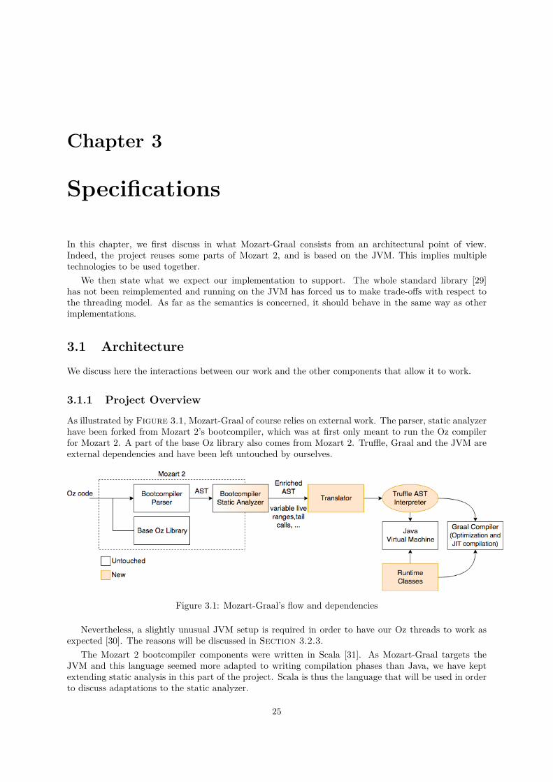
3.1 Mozart-Graal’s flow and dependencies . . . . . . . . . . . . . . . . . . . . . . . . . . . . . 25
4.1 Only one level of indirection is possible when at least one variable is single . . . . . . . . . 304.2 More indirection is however necessary for other cases . . . . . . . . . . . . . . . . . . . . . 304.3 Binding linked variables in Mozart-Graal . . . . . . . . . . . . . . . . . . . . . . . . . . . 304.4 Multiplicity frequencies when variables get bound in sample programs . . . . . . . . . . . 314.5 AST of last example from Listing 4.4 . . . . . . . . . . . . . . . . . . . . . . . . . . . . . 334.6 Illustration of both frame linked list and environment selection. Frames are represented
as containing their arguments and slots for local variables . . . . . . . . . . . . . . . . . . 364.7 Tail call optimization control flow example . . . . . . . . . . . . . . . . . . . . . . . . . . . 43
5.1 Self tail call optimization illustration . . . . . . . . . . . . . . . . . . . . . . . . . . . . . . 505.2 Graal’s point of view while stuck into tail calls is not ideal . . . . . . . . . . . . . . . . . . 575.3 On Stack Replacement to allow earlier optimization . . . . . . . . . . . . . . . . . . . . . 58
6.1 Iteration times of Add with and without OSR and self tail call optimization . . . . . . . . 666.2 Mean iteration times of Project2014 with and without OSR and self tail call optimization 676.3 Mean iteration times of the different variants of unification and equality tests . . . . . . . 686.4 Distributions of iteration times for all benchmarks with and without inlining . . . . . . . 696.5 Distributions of iteration times for all benchmarks with and without builtins splitting . . 706.6 Visualization for execution passing in producer-consumer applications . . . . . . . . . . . 716.7 Mean iteration times for Sieve under different parameter sets and implementations . . . . 726.8 Evolution of peak iteration times for the Sieve when increasing N on Mozart-Graal and
Mozart 1 . . . . . . . . . . . . . . . . . . . . . . . . . . . . . . . . . . . . . . . . . . . . . . 736.9 Mean iteration times for Project2014 on Mozart 1, Mozart 2 and Mozart-Graal on the
joie.dj.oz and strugala.dj.oz partitions . . . . . . . . . . . . . . . . . . . . . . . . . . 746.10 Distribution of iteration times on Mozart 1, Mozart 2 and Mozart-Graal for all the bench-
marks but Project2014 . . . . . . . . . . . . . . . . . . . . . . . . . . . . . . . . . . . . . 746.11 Heap size measures for all benchmarks and implementations . . . . . . . . . . . . . . . . . 75
A.1 Noise introduced by time measurements . . . . . . . . . . . . . . . . . . . . . . . . . . . . 85A.2 Difference in heap size around data structure allocation . . . . . . . . . . . . . . . . . . . 87A.3 Graal IR obtained for Add without self tail calls and without OSR . . . . . . . . . . . . . 88A.4 Graal IR obtained for Add with self tail calls and with OSR . . . . . . . . . . . . . . . . . 89A.5 Graal IR obtained for Add without self tail calls but with OSR (1st phase) . . . . . . . . . 90
11
A.6 Graal IR obtained for Add without self tail calls but with OSR (2nd phase) . . . . . . . . 91
12
Listings
2.1 Oz expression example . . . . . . . . . . . . . . . . . . . . . . . . . . . . . . . . . . . . . . 192.2 Example of an AddNode specialization for the Integer type . . . . . . . . . . . . . . . . . 202.3 Truffle implementation of the Oz “+” operator . . . . . . . . . . . . . . . . . . . . . . . . 212.4 Type system description of our implementation . . . . . . . . . . . . . . . . . . . . . . . . 222.5 Oz scenario around AddNode rewriting . . . . . . . . . . . . . . . . . . . . . . . . . . . . . 22
4.1 Hazards of linking using circular lists (Colors denote equivalent variables) . . . . . . . . . 314.2 Pathological case for variable linking with complexity O(N2) . . . . . . . . . . . . . . . . 324.3 Truffle nodes instantiating variables and accessing them . . . . . . . . . . . . . . . . . . . 324.4 Examples of Oz nodes . . . . . . . . . . . . . . . . . . . . . . . . . . . . . . . . . . . . . . 334.5 Truffle implementation for IfNode . . . . . . . . . . . . . . . . . . . . . . . . . . . . . . . 334.6 Truffle skeleton for the UnifyNode . . . . . . . . . . . . . . . . . . . . . . . . . . . . . . . 344.7 A Truffle call node for Oz procedures . . . . . . . . . . . . . . . . . . . . . . . . . . . . . . 374.8 Excerpt from the DynamicObjectBasic placeholder class from Truffle . . . . . . . . . . . 384.9 A specialization for handling calls to Oz object methods . . . . . . . . . . . . . . . . . . . 394.10 The AddNode builtin, corresponding to the “+” operator . . . . . . . . . . . . . . . . . . . 404.11 Example of how tail calls behave . . . . . . . . . . . . . . . . . . . . . . . . . . . . . . . . 434.12 Truffle implementation of the tail call mechanism . . . . . . . . . . . . . . . . . . . . . . . 444.13 Tail function code . . . . . . . . . . . . . . . . . . . . . . . . . . . . . . . . . . . . . . . . 454.14 Output of bootcompiler . . . . . . . . . . . . . . . . . . . . . . . . . . . . . . . . . . . . . 454.15 Desirable output . . . . . . . . . . . . . . . . . . . . . . . . . . . . . . . . . . . . . . . . . 454.16 exprToBindStatement handling expressions having equivalent statements . . . . . . . . . . 464.17 Cases of tail functions that are still undetected . . . . . . . . . . . . . . . . . . . . . . . . 464.18 Example of result record partial unwrapping . . . . . . . . . . . . . . . . . . . . . . . . . . 47
5.1 Truffle nodes for handling self tail calls . . . . . . . . . . . . . . . . . . . . . . . . . . . . 515.2 Example benefiting from early FrameSlot clearing . . . . . . . . . . . . . . . . . . . . . . 515.3 Truffle node for clearing unused slots . . . . . . . . . . . . . . . . . . . . . . . . . . . . . . 535.4 Trivial Oz example benefiting from polymorphic inline caching and AST inlining . . . . . 555.5 Truffle CallNode for Oz procedures with both polymorphic inline caching and AST inlining 56
6.1 Code of the Bounded Buffer . . . . . . . . . . . . . . . . . . . . . . . . . . . . . . . . . . . 70
A.1 Add program . . . . . . . . . . . . . . . . . . . . . . . . . . . . . . . . . . . . . . . . . . . 86A.2 Variant of Add with declared variables . . . . . . . . . . . . . . . . . . . . . . . . . . . . . 86
13

14
Acronyms
API Application Programming Interface. 22, 27, 28, 38, 49, 54, 58
AST Abstract Syntax Tree. 19–21, 23, 24, 26, 27, 31, 32, 34–37, 39, 42, 45, 49, 56, 58, 65, 78, 79
DSL Domain-Specific Language. 21–23, 56, 79
EA Escape Analysis. 23
IR Internal Representation. 22, 62, 66
JIT Just-In-Time. 18, 20, 22, 28, 30, 64
JVM Java Virtual Machine. 17, 23–29, 42, 61, 74
OS Operating System. 27, 28
OSR On Stack Replacement. 57, 58, 65–67
PEA Partial Escape Analysis. 23
PIC Polymorphic Inline Cache. 69
SSA Static Single Assignment. 22
SSH Secure Shell. 61
VM Virtual Machine. 17
15

16
Chapter 1
Introduction
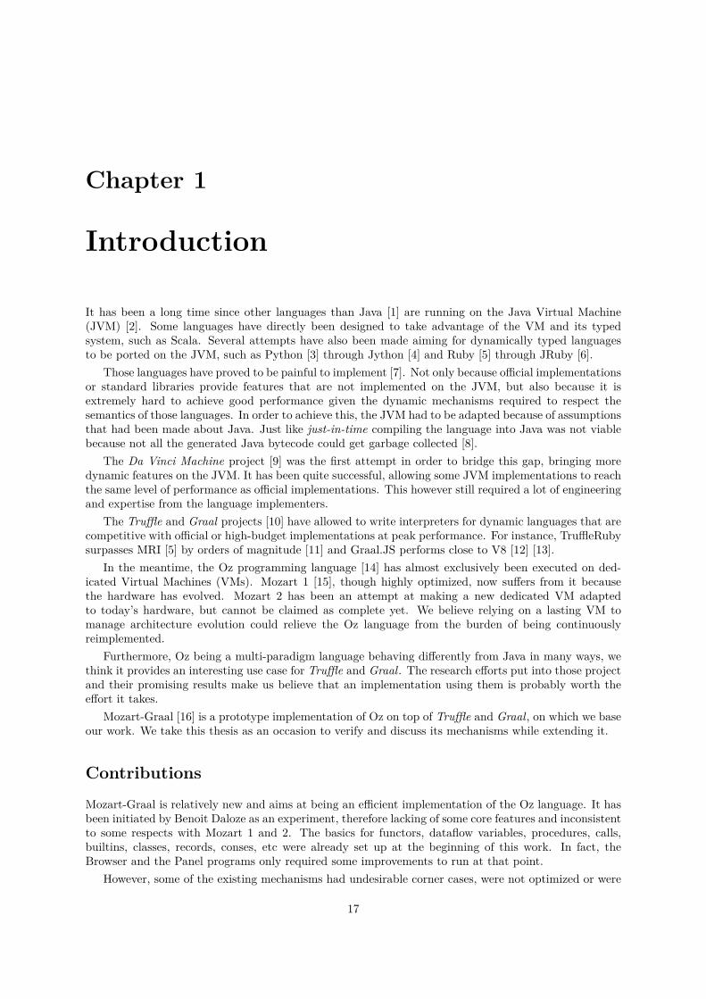
It has been a long time since other languages than Java [1] are running on the Java Virtual Machine(JVM) [2]. Some languages have directly been designed to take advantage of the VM and its typedsystem, such as Scala. Several attempts have also been made aiming for dynamically typed languagesto be ported on the JVM, such as Python [3] through Jython [4] and Ruby [5] through JRuby [6].
Those languages have proved to be painful to implement [7]. Not only because official implementationsor standard libraries provide features that are not implemented on the JVM, but also because it isextremely hard to achieve good performance given the dynamic mechanisms required to respect thesemantics of those languages. In order to achieve this, the JVM had to be adapted because of assumptionsthat had been made about Java. Just like just-in-time compiling the language into Java was not viablebecause not all the generated Java bytecode could get garbage collected [8].
The Da Vinci Machine project [9] was the first attempt in order to bridge this gap, bringing moredynamic features on the JVM. It has been quite successful, allowing some JVM implementations to reachthe same level of performance as official implementations. This however still required a lot of engineeringand expertise from the language implementers.
The Truffle and Graal projects [10] have allowed to write interpreters for dynamic languages that arecompetitive with official or high-budget implementations at peak performance. For instance, TruffleRubysurpasses MRI [5] by orders of magnitude [11] and Graal.JS performs close to V8 [12] [13].
In the meantime, the Oz programming language [14] has almost exclusively been executed on ded-icated Virtual Machines (VMs). Mozart 1 [15], though highly optimized, now suffers from it becausethe hardware has evolved. Mozart 2 has been an attempt at making a new dedicated VM adaptedto today’s hardware, but cannot be claimed as complete yet. We believe relying on a lasting VM tomanage architecture evolution could relieve the Oz language from the burden of being continuouslyreimplemented.
Furthermore, Oz being a multi-paradigm language behaving differently from Java in many ways, wethink it provides an interesting use case for Truffle and Graal. The research efforts put into those projectand their promising results make us believe that an implementation using them is probably worth theeffort it takes.
Mozart-Graal [16] is a prototype implementation of Oz on top of Truffle and Graal, on which we baseour work. We take this thesis as an occasion to verify and discuss its mechanisms while extending it.
Contributions
Mozart-Graal is relatively new and aims at being an efficient implementation of the Oz language. It hasbeen initiated by Benoit Daloze as an experiment, therefore lacking of some core features and inconsistentto some respects with Mozart 1 and 2. The basics for functors, dataflow variables, procedures, calls,builtins, classes, records, conses, etc were already set up at the beginning of this work. In fact, theBrowser and the Panel programs only required some improvements to run at that point.
However, some of the existing mechanisms had undesirable corner cases, were not optimized or were
17
not garbage-collection-friendly. We have thus mainly devoted our efforts to improving the correctnessand the performance of the implementation.
Static analysis has thus been extended to optimize tail calls and reduce variable usages and lifetimes.The mechanism for handling external environments has been revamped to become garbage-collection-friendly. Dataflow variables, unification and equality testing have been corrected. Method calls now ben-efit from polymorphic inline caches and calls to inexistent methods are well redirected to the otherwisefallback method and are even optimized. Different strategies have also been explored to allow earlierJust-In-Time (JIT) compilation. Other modifications have occurred in the process, such as the imple-mentation of new builtins or the inlining of operators, and more improvement ideas have been generated.
All the modifications can be found in a GitHub repository [17]. Part of them have been merged inthe official Mozart-Graal repository [16] and the others are meant to be in a short future. The totalmodifications consist of 52 commits providing 3 thousands new lines as a result of 4 thousands additionsand 1 thousand deletions spread in more than a hundred files.
In order to evaluate the improvements made, a tool has been written in Python for running Ozprograms and aggregating their outputs. It also allows for other implementations to run those. This toolis available in a dedicated GitHub repository [18] along with some benchmark programs and a Jupyternotebook [19] for data visualization.
Structure
First, the main principles about self-optimizing interpreters, Truffle, Graal, their roles and general speci-ficities will be introduced in Chapter 2.
A more refined idea of what has been accomplished in Mozart-Graal is provided right after in Chap-ter 3. Both in terms of the structure, and in terms of the language that has been implemented.
Chapter 4 then proposes to have a look at the mapping of some key concepts from Oz to Trufflewithout considering performance. This should allow to grasp the primitives necessary to write languagesimplementations running with Truffle.
Chapter 5 is then all about specific optimizations that are now performed when running codeon Mozart-Graal. The first part details improvements in performance and memory management thatrely on information provided by the static analysis of our compiler whereas the second part describesoptimizations relying on Graal or making its job easier.
Chapter 6 evaluates the different optimizations and compares Mozart-Graal to Mozart 1 and 2,exposing both quantitative data collected on benchmarks and some of the Graal compiler output. Somelimitations of the actual code and tools behind have been encountered and will be detailed.
Chapter 7 sets out some possible future developments.
18
Chapter 2
Main Principles
In this chapter, we will discuss briefly what Truffle and Graal are, and what are the principles behindthem. We will see what self-optimizing Abstract Syntax Tree (AST) interpreters are, how Truffle allowswriting them easier. Finally, we will see what makes Graal special and how it can take advantage fromsuch interpreters being written with Truffle.
2.1 Self-Optimizing AST Interpreters
We consider an AST interpreter as a tree of node objects that can be evaluated within some executionenvironment. AST interpreters are a very common way to implement a language. We will see how theywork in their simplest form, and how they can take advantage from runtime execution profiling to makethemselves considerably faster.
2.1.1 Classical AST Interpreters
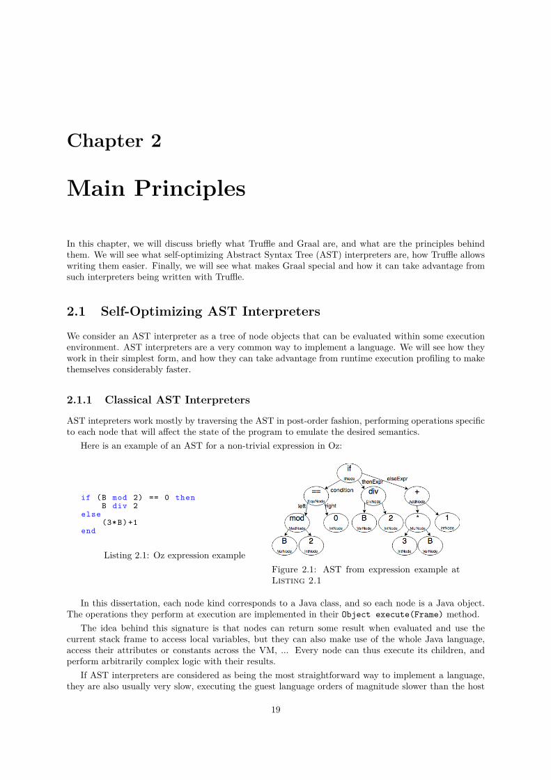
AST intepreters work mostly by traversing the AST in post-order fashion, performing operations specificto each node that will affect the state of the program to emulate the desired semantics.
Here is an example of an AST for a non-trivial expression in Oz:
if (B mod 2) == 0 thenB div 2
else(3*B)+1
end
Listing 2.1: Oz expression exampleFigure 2.1: AST from expression example atListing 2.1
In this dissertation, each node kind corresponds to a Java class, and so each node is a Java object.The operations they perform at execution are implemented in their Object execute(Frame) method.
The idea behind this signature is that nodes can return some result when evaluated and use thecurrent stack frame to access local variables, but they can also make use of the whole Java language,access their attributes or constants across the VM, ... Every node can thus execute its children, andperform arbitrarily complex logic with their results.
If AST interpreters are considered as being the most straightforward way to implement a language,they are also usually very slow, executing the guest language orders of magnitude slower than the host
19
language. A lot of interpreted languages suffer from poor performances on the JVM because they arebasically too rich. Their nodes therefore have to perform a lot of checks and dispatches, even in the mosttrivial and performance-critical parts, in order to be correct every time.
2.1.2 Self-Optimizing AST Interpreters
Self-optimizing interpreters are interpreters taking advantage of the execution profile in order to optimizethemselves [20].
The first idea that allows those interpreters to be optimized is that there are conditions under whichfor some node instances, the execute method could do simplified work. If a “+” node in the code alwaysadds two integers for instance, there is no need to make complex dispatching on object types.
The second idea, the one making self-optimization fit that well into AST interpreters is that we candiscover at runtime under which conditions every node is being executed from the beginning of execution.It is therefore possible to avoid hard work as long as the preconditions of lighter variants are fulfilled.
Nodes can also have their own state depending on what they have received in their previous usages,and conditions about it can be expressed in guards. This is especially useful for implementing mechanismssimilar to polymorphic inline caches for instance. Those are motivated by the fact some call nodes couldobserve a small set of types for the whole execution of a program. Information about methods can thusbe cached most of the time.
A simple way of implementing self-optimizing interpreters is presented in [20]. The language imple-menter basically provides several node classes (i.e. specializations) for each single feature, each special-ization checking the preconditions it relies on still hold before executing. If this is not the case anymore,it must replace itself with another specialization and let it execute instead.
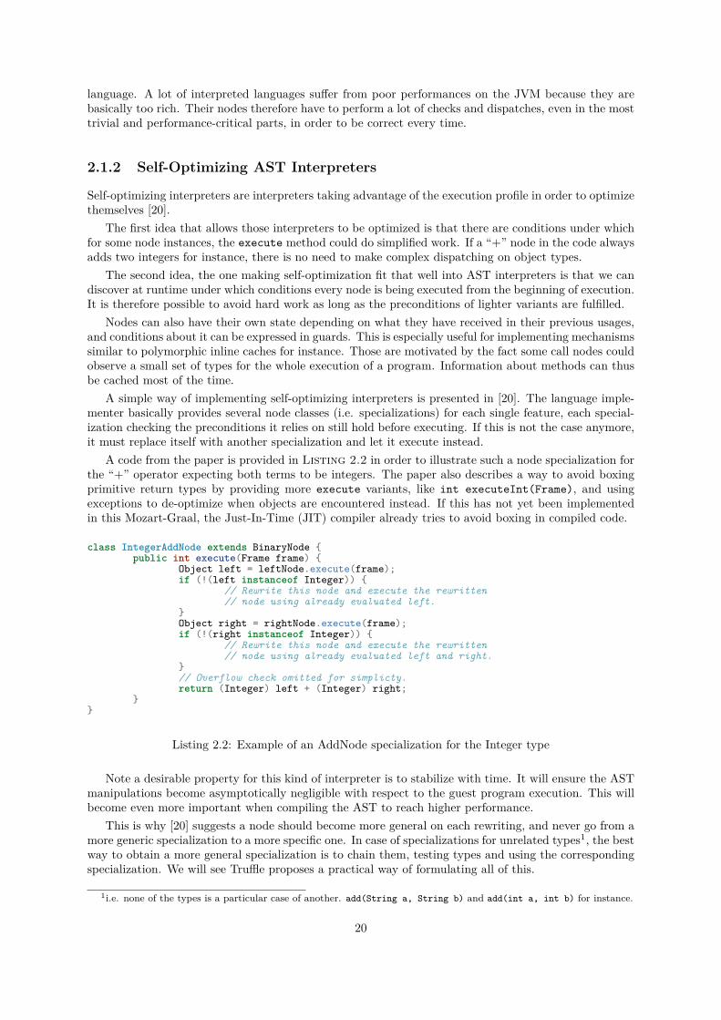
A code from the paper is provided in Listing 2.2 in order to illustrate such a node specialization forthe “+” operator expecting both terms to be integers. The paper also describes a way to avoid boxingprimitive return types by providing more execute variants, like int executeInt(Frame), and usingexceptions to de-optimize when objects are encountered instead. If this has not yet been implementedin this Mozart-Graal, the Just-In-Time (JIT) compiler already tries to avoid boxing in compiled code.
class IntegerAddNode extends BinaryNode {public int execute(Frame frame) {
Object left = leftNode.execute(frame);if (!(left instanceof Integer)) {
// Rewrite this node and execute the rewritten// node using already evaluated left.
}Object right = rightNode.execute(frame);if (!(right instanceof Integer)) {
// Rewrite this node and execute the rewritten// node using already evaluated left and right.
}// Overflow check omitted for simplicty.return (Integer) left + (Integer) right;
}}
Listing 2.2: Example of an AddNode specialization for the Integer type
Note a desirable property for this kind of interpreter is to stabilize with time. It will ensure the ASTmanipulations become asymptotically negligible with respect to the guest program execution. This willbecome even more important when compiling the AST to reach higher performance.
This is why [20] suggests a node should become more general on each rewriting, and never go from amore generic specialization to a more specific one. In case of specializations for unrelated types1, the bestway to obtain a more general specialization is to chain them, testing types and using the correspondingspecialization. We will see Truffle proposes a practical way of formulating all of this.
1i.e. none of the types is a particular case of another. add(String a, String b) and add(int a, int b) for instance.
20
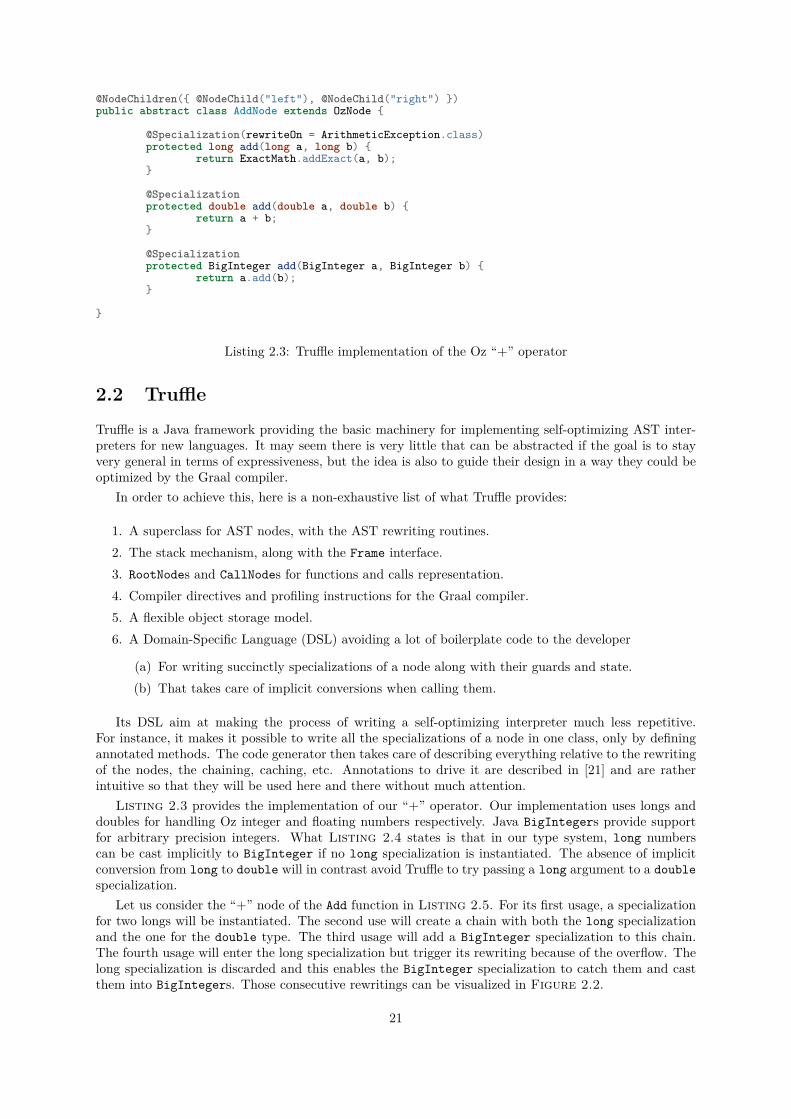
@NodeChildren({ @NodeChild("left"), @NodeChild("right") })public abstract class AddNode extends OzNode {
@Specialization(rewriteOn = ArithmeticException.class)protected long add(long a, long b) {
return ExactMath.addExact(a, b);}
@Specializationprotected double add(double a, double b) {
return a + b;}
@Specializationprotected BigInteger add(BigInteger a, BigInteger b) {
return a.add(b);}
}
Listing 2.3: Truffle implementation of the Oz “+” operator
2.2 Truffle
Truffle is a Java framework providing the basic machinery for implementing self-optimizing AST inter-preters for new languages. It may seem there is very little that can be abstracted if the goal is to stayvery general in terms of expressiveness, but the idea is also to guide their design in a way they could beoptimized by the Graal compiler.
In order to achieve this, here is a non-exhaustive list of what Truffle provides:
1. A superclass for AST nodes, with the AST rewriting routines.2. The stack mechanism, along with the Frame interface.3. RootNodes and CallNodes for functions and calls representation.4. Compiler directives and profiling instructions for the Graal compiler.5. A flexible object storage model.6. A Domain-Specific Language (DSL) avoiding a lot of boilerplate code to the developer
(a) For writing succinctly specializations of a node along with their guards and state.(b) That takes care of implicit conversions when calling them.
Its DSL aim at making the process of writing a self-optimizing interpreter much less repetitive.For instance, it makes it possible to write all the specializations of a node in one class, only by definingannotated methods. The code generator then takes care of describing everything relative to the rewritingof the nodes, the chaining, caching, etc. Annotations to drive it are described in [21] and are ratherintuitive so that they will be used here and there without much attention.
Listing 2.3 provides the implementation of our “+” operator. Our implementation uses longs anddoubles for handling Oz integer and floating numbers respectively. Java BigIntegers provide supportfor arbitrary precision integers. What Listing 2.4 states is that in our type system, long numberscan be cast implicitly to BigInteger if no long specialization is instantiated. The absence of implicitconversion from long to double will in contrast avoid Truffle to try passing a long argument to a doublespecialization.
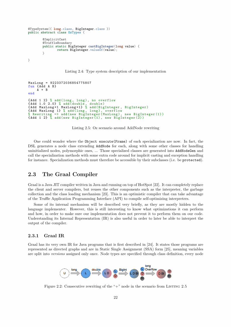
Let us consider the “+” node of the Add function in Listing 2.5. For its first usage, a specializationfor two longs will be instantiated. The second use will create a chain with both the long specializationand the one for the double type. The third usage will add a BigInteger specialization to this chain.The fourth usage will enter the long specialization but trigger its rewriting because of the overflow. Thelong specialization is discarded and this enables the BigInteger specialization to catch them and castthem into BigIntegers. Those consecutive rewritings can be visualized in Figure 2.2.
21
@TypeSystem({ long.class, BigInteger.class })public abstract class OzTypes {
@ImplicitCast@TruffleBoundarypublic static BigInteger castBigInteger(long value) {
return BigInteger.valueOf(value);}
}
Listing 2.4: Type system description of our implementation
MaxLong = 9223372036854775807fun {Add A B}
A + Bend
{Add 1 2} % add(long , long), no overflow{Add 1.0 2.0} % add(double , double ){Add MaxLong +1 MaxLong +1} % add(BigInteger , BigInteger ){Add MaxLong 1} % add(long , long), overflow% Rewriting => add(new BigInteger ( MaxLong ), new BigInteger (1)){Add 1 2} % add(new BigInteger (1) , new BigInteger (2))
Listing 2.5: Oz scenario around AddNode rewriting
One could wonder where the Object execute(Frame) of each specialization are now. In fact, theDSL generates a node class extending AddNode for each, along with some other classes for handlinguninitialized nodes, polymorphic ones, ... Those specialized classes are generated into AddNodeGen andcall the specialization methods with some extra code around for implicit casting and exception handlingfor instance. Specialization methods must therefore be accessible by their subclasses (i.e. be protected).
2.3 The Graal Compiler
Graal is a Java JIT compiler written in Java and running on top of HotSpot [22]. It can completely replacethe client and server compilers, but reuses the other components such as the interpreter, the garbagecollection and the class loading mechanism [23]. This is an optimistic compiler that can take advantageof the Truffle Application Programming Interface (API) to compile self-optimizing interpreters.
Some of its internal mechanism will be described very briefly, as they are mostly hidden to thelanguage implementer. However, this is still interesting to know what optimizations it can performand how, in order to make sure our implementation does not prevent it to perform them on our code.Understanding its Internal Representation (IR) is also useful in order to later be able to interpret theoutput of the compiler.
2.3.1 Graal IR
Graal has its very own IR for Java programs that is first described in [24]. It states those programs arerepresented as directed graphs and are in Static Single Assignment (SSA) form [25], meaning variablesare split into versions assigned only once. Node types are specified through class definition, every node
Figure 2.2: Consecutive rewriting of the “+” node in the scenario from Listing 2.5
22
class extending the Node class. (Not the same as Truffle’s one)The graph is created by specifying two types of edges: control flow (successor) edges and data flow
(input) edges. Control flow edges only ensure control flow between loops, conditions, etc, whereas dataflow edges express the input data of every operation. The latter may as well be used for expressingscheduling dependencies.
The Node class provides methods for easily redirecting edges or replace the node in the surroundinggraph. As a side note, various interfaces are available on them in order to perform optimizations suchas simplification and lowering. This is preferred to the visitor pattern to preserve extensibility.
The order specified by control flow edges is strict. However, nodes with only data flow edges canbe moved between their dependencies and nodes depending on them and are said to be floating nodes.Flexibility in their scheduling allows to not have to maintain a correct schedule at all time and todetermine it later with specific heuristics.
This also allows for code-motion based optimization to be implemented easily. Most floating nodesare for instance candidate to global value numbering [26], which allows for merging nodes that haveredundant computations.
In order to run compiled Java class files, the Graal compiler first has to convert them into itsintermediate representation. For simplicity however, only reducible loops are handled by the conversion.This is legitimated by the fact Java code only generates reducible loops but also means some bytecodeobfuscation can render methods to be unusable by the Graal compiler, therefore forcing them to run ininterpreter mode.
2.3.2 Optimization
Part of what allows Graal to compile efficiently dynamically typed languages is that it is actually goodat optimizing and compiling Java, and therefore also other statically typed JVM languages.
The other part is due to the principles of self-optimizing interpreters and the hints language imple-menters can provide by annotating them. The former allow simpler routines to be compiled as long asthey are sufficient for the execution. The latter helps the compiler acquiring additional knowledge aboutthe code.
2.3.2.1 Optimizing Java Code
Graal still shares a lot with the HotSpot Server Compiler. One of its main improvement over the latteris however an analysis named Partial Escape Analysis (PEA). Escape Analysis (EA) allows a compiler todetermine whether an object is accessible outside the allocating method or thread [23]. PEA has bettergranularity in that it makes the distinction between different branches.
In the HotSpot Server Compiler, EA allows stack allocation, scalar replacement and lock elision totake place [27]. Stack allocation allows objects that are not put into Java fields to be allocated on thestack. scalar replacement allows objects that are only used locally to be replaced by their useful fieldsallocated on the stack. This is thus stronger than stack allocation. Lock elision avoids unnecessarysynchronizations when the object has not yet been able to escape to other threads.
Those optimizations benefit from method inlining, which provides more opportunities to avoid allo-cating complete objects passed as arguments to inlined function, etc. Refining the escape analysis tothe branch level is another opportunity to make them more efficient as well, for instance only allocatingobjects and acquiring locks on them in the branches they can escape from.
It is however important to note that the compilation process is expensive. It is therefore valuable if theimplementer can help the compiler to detect critical parts of programs and to perform some optimizations.Truffle enables this interaction and provides a DSL making it easier to write PEA-friendly code.
2.3.2.2 Truffle Compiler Directives and Annotations
Truffle allows to tag values to be considered as constants within a compilation even though referencesto them escape. This happens on the AST nodes we write for instance. Node children are considered as
23
constant for compilation, which allows the compiler to directly look through the execute calls, considerthe methods behind and reason more globally.
The language implementer can also provide other directives to the compiler, stating for instance tonever compile some branches, or only if they have never been entered. He can also collect and injectbranch probabilities into the AST or specify branches to only be taken in interpreter or in compiled mode.Loops can also be tagged to unroll whenever their number of iteration can be considered as constant.
Finally, all those mechanisms can be coupled with node state to specialize some general routine tothe only values or types it has received that can then be considered as constant locally. This is definitelywhere dynamic languages can get the most from the JVM.
All of this is possible and made easy using Truffle. This will be discussed in Section 5.2.
2.3.3 Deoptimization
Such speculative optimization is however only enabled by the concept of deoptimization [28]. Wheneverpreconditions of compiled code are invalidated it is not safe to execute anymore. When encounteringguards evaluating to false before such now-invalid sections of code or explicit deoptimization instruc-tions, the interpreter thus has to take over the execution.
This deoptimization phenomenon may happen because of the language implementation using Truffle,for instance when none of the instantiated specializations can handle the actual parameters or when abranch that is not compiled needs to be taken, or that the AST needs to be rewritten. It may howeverhappen for less visible reasons, like when a Java class is loaded, providing a second implementation fora method that was before considered as having only one implementation.
For deoptimization to work, it must be possible to reconstruct the state of the VM from the stateof the physical machine at deoptimization points. This is what is achieved through framestates. Theybasically contain the information about what the interpreter must do in order to catch up what hadalready been done by the compiled code, without introducing side-effects. This of course includes abytecode pointer, values in the stack frame, but can also describe objects to be allocated in case theywere not.
24
Chapter 3
Specifications
In this chapter, we first discuss in what Mozart-Graal consists from an architectural point of view.Indeed, the project reuses some parts of Mozart 2, and is based on the JVM. This implies multipletechnologies to be used together.
We then state what we expect our implementation to support. The whole standard library [29]has not been reimplemented and running on the JVM has forced us to make trade-offs with respect tothe threading model. As far as the semantics is concerned, it should behave in the same way as otherimplementations.
3.1 Architecture
We discuss here the interactions between our work and the other components that allow it to work.
3.1.1 Project Overview
As illustrated by Figure 3.1, Mozart-Graal of course relies on external work. The parser, static analyzerhave been forked from Mozart 2’s bootcompiler, which was at first only meant to run the Oz compilerfor Mozart 2. A part of the base Oz library also comes from Mozart 2. Truffle, Graal and the JVM areexternal dependencies and have been left untouched by ourselves.
Figure 3.1: Mozart-Graal’s flow and dependencies
Nevertheless, a slightly unusual JVM setup is required in order to have our Oz threads to work asexpected [30]. The reasons will be discussed in Section 3.2.3.
The Mozart 2 bootcompiler components were written in Scala [31]. As Mozart-Graal targets theJVM and this language seemed more adapted to writing compilation phases than Java, we have keptextending static analysis in this part of the project. Scala is thus the language that will be used in orderto discuss adaptations to the static analyzer.
25
The Translator is a Java class that generates Truffle AST nodes (i.e. the structure interpreting theOz program) from the output of Mozart 2’s bootcompiler. Those components are written in Java, sothis is the language that will be used to described them in this dissertation.
3.1.2 Parsing and Static Analysis
The parser has mainly been left untouched. The static analyzer has however been modified here andthere. Let us have a look at each phase: (–: as-is from Mozart 2, ~: adapted, +: added)
– Identifier resolution, that generates a unique identifier for each variable declaration in the currentfunctor, and that links every occurrence of that variable in the AST to it.
~ Desugaring, that transforms functors, classes, functions more primitives constructs of the language.It has been extended in order to push the assignments of result variables as far as possible inthe body of procedures in order to make detection of tail calls easier. This will be detailed inSection 4.4.3.
– Constant folding, that replaces occurrences of builtins by direct references.– Unnesting, that handles the nesting marker $ in procedure calls.+ Tail call detection, that tags tail calls in order for the Translator to create adequate interpreter
nodes.This will be discussed in Section 4.4.3 as well.
+ On stack variables detection, tagging local variables that are not required to be instantiated asdataflow variables.This optimization will be discussed in Section 5.1.2.
+ Frame slot clearing, that tags statements and expressions before or after which local variables couldbe forgotten in order to free references as soon as possible.This is an optimization and will therefore be discussed in Section 5.1.3.
3.1.3 Tests
Some Oz tests have been kept from Mozart 2 (platform-test/base/) for base types and concepts suchas numbers, procedures, dictionaries, records, types, exceptions, conversions, threads and laziness. Someothers may pass, but as the accent has not been put on completeness of the implementation, most willnot. Either because they try to test syntactic structures that are not handled by Mozart 2’s bootcompilerparser, or because they make use of unimplemented builtins.
For generic tail calls and cyclic unification, Oz unit tests have also been added there. They shouldthus lead to stack overflows or block whenever cases are missed. For some additions to static analysis,the behavior is by definition even harder to observe in Oz. Special builtins have been introduced in theDebug functor that allow ensuring variables are allocated on stack, or that references have been freed.In order not to influence the static analysis itself, variable names are provided as atoms.
All the tests known to pass are executed when no argument is provided to the ./oz executable.Furthermore, the implementation should correctly run examples such as the Browser and the Panellocated in examples/, as well as the 2014 Oz Music Project [32].
3.2 Language Specifications
It has been tried to make the implementation as compliant with existing resources as possible. Thereare however some differences due to actual limitations of the JVM and the fact implementing the wholestandard library would have taken too much time. In this section, we will detail the differences betweenOzT, the implemented language, in contrast to the original Oz language.
26
3.2.1 The Semantics
Mozart-Graal tries to make OzT follow Oz’ semantics, provided by [33, chap. 13], and seems to almostachieve it. Some hints about it will be provided in Chapter 4.
The main difference is that OzT tries to take advantage from evaluating expressions in the ASTto values directly rather than associating them with dataflow variables systematically as the Oz kernellanguage would. It means that rather than being desugared down to the Oz kernel language, OzTprograms are rather transformed to some intermediate believed to only have imperceptible differenceswith Oz, but also to be more efficient in terms of number of instantiated variables. We could call thislanguage OzT’s kernel language.
This therefore puts some distance between the formal version of the Oz language and OzT, sincevalues can now be provided to any operation. We will however help ourselves to close this gap inthe implementation, by bringing a unified reasoning on both variables and values. Also, rather thanintroducing a supplementary stack of variables for the nested expressions of our “kernel language”, eachof those could mostly be seen as introducing a single-use variable computed before the surroundingoperation, and accessed at the place of the expression only.
Finally, if the illusion is not perfect yet, this is because there remains some minor edge cases thatare not stated specifically in the transformation, making OzT’s kernel language stand a little too faithfulwith respect to the user input compared to Oz’s kernel language. This is however a matter of time.Those edge cases are provided with other bugs in Appendix B.
3.2.2 Builtins
OzT builtins are decomposed in intrinsic and plain-Oz builtins. The former had to be rewritten usingTruffle, as discussed later in Section 4.3.9 while the latter have been forked from Mozart 2’s standardlibrary. If it has been tried to provide a sufficient kernel some interesting projects to run with the currentimplementation, it is far from being complete.
In order to make Mozart-Graal maintainers’ lives easier, placeholder node classes have been generatedfor all of them, so when a builtin is missing, an exception is thrown at runtime and specializations caneasily be added to the already existing node class.
3.2.3 Threads
For some reason, OzT’s “threads” are not equivalent to Oz’ ones. Let us first define different flavors forconcurrency. If there seems to be no consensus as to how every concept should be called in the literatureand in APIs, this is how each of those concepts will be referred to in this dissertation:
Threads allow different tasks to run concurrently, and are expected to be scheduled in a fair manner[33]. (they can therefore be suspended at any moment by the scheduler, and are therefore qualifiedas “preemptive”) There is also a notion of priority between different threads.
Most Operating Systems (OSs) provide such a system but limit the number of threads per process.Having to interact through system calls and OS-level context switching induce a large overhead.Language implementations therefore try to provide more adapted and lightweight mechanisms.
(Symmetric) coroutines are basically non-preemptive threads [34]. Scheduling must be specifiedexplicitly within a coroutine by releasing the execution through a yield operation. This is why theyare said to provide “cooperative concurrency”.
Asymmetric coroutines are similar to symmetric coroutines except they must return control to theirinvoker [34]. It is however possible for them to invoke other coroutines before doing so.
Oz’ approach to concurrency is all about preemptive threads running in a single OS thread. On astandard JVM, however, only OS threads are available. Let us first have an overview of how state-of-the-art JVM interpreters and libraries achieve their kind of concurrency.
27
JRuby directly uses OS threads as asymmetric and symmetric coroutines [35]. This thus means only alimited number of them can be spawned and they induce a large overhead for context switching.
Akka [36] proposes a strong foundation for concurrent and distributed applications, but only makes useof OS threads as well.
Quasar [37] implements lightweight threads by instrumenting bytecode, either at compile-time or atruntime, in order to restore the stack and jump back to the instruction it was executing. [38]
Therefore, those two options would be available:
1. Either spawn an OS thread for every Oz thread, therefore limiting them in number and bringinga huge overhead for context switching. But such threads are preemptive and may benefit frommulti-core CPUs.
2. Either simulate lightweight threads via code instrumentation to save the stack, restore it and jumpback at the right location.
Luckily for us, a third options exists and consists in a modified JVM with Graal and added supportfor coroutines, very close to what is described in [39]. It seems better to rely on it.
Indeed, if the first solution seems very appealing, the fact we could only spawn a limited number ofthreads (around two thousand) is not acceptable. Some Oz programs have a strong tendency to createa lot of them for very lightweight concurrent tasks, which would therefore simply not work.
The second option is not really viable either because such instrumentation would be very intrusiveand would most likely interfere with the analysis done by the JIT compiler.
Though the most adapted, the third solution would ideally still imply to add a preemption mechanism.Because the JVM does not provide any API for signals, this would therefore require to add costlytiming checks within the program. At each tail call for instance. As it may lead to severe performancedegradation and was not necessary in observed programs, it has been decided not to handle preemptionfor now.
This basically means that a program that never waits on any variable will never yield the executionto any other thread, and therefore that threads may starve. A simple example is for instance a non-lazyinteger stream generator, or a function simply calling itself forever.
Such functions are usually not advised, but may be legitimate. In order to provide a temporarysolution, OzT provides the {Delay 0} call. It is optimized to simply cause the current thread to yieldwithout more overhead.
28
Chapter 4
Mapping Oz concepts to Truffle
In this chapter, we will consider how Oz concepts are mapped into Truffle. This mapping aims at beingas simple as possible while respecting the semantics and avoiding corner cases.
The variables are first discussed, along with the local environment, and how the dataflow is handled.We then see how procedures are mapped in Mozart-Graal by assembling mechanisms handling theirarguments, external environment, code and finally their calls.
Having those allows us to discuss how the base Oz types and the builtin procedures are implemented.The mapping the unification, equality testing and pattern matching is then addressed.
Finally, this chapter ends with the translation of tail calls and their detection at static analysis.
4.1 Oz Dataflow Variables
Dataflow variables do not exist by default on the JVM, but are at the core of the Oz language and itsvery particular semantics. Those variables can only be assigned once. Indeed, the first unification ofa variable with a value will assign it. Further unifications will instead unify its value with the othermember. This last mechanism will be discussed in Section 4.4.
Whenever an operation needs a value from an unbound variable, it will have to wait onto it untilanother thread binds it.
It is also possible to unify two unbound variables. In that case, both variables should be linked sothat they become indistinguishable from each other. This means that binding one should bind themboth, and any other variable bound with one of them.local A B in
thread {Wait B} {Show ’B is bound ’} endA = BA = 3 % A and B are now have value "3"% "B is bound" is eventually printed
end
The natural way of implementing this linking mechanism between two variables is to set one tohave the other as value. We will call the variable pointing to the other the alias, and the other therepresentative. When an operation is attempted on an alias, it must be performed on its representativein order for the effects to be perceptible by both. Considering the above case, assigning A to 3 or waitingon it would otherwise be unnoticeable through B.
It is possible to obtain bigger sets of equivalent variables. Because linking two sets of equivalentvariables must always link one of the representatives to the other, by construction, any bigger set ofequivalent variable only has one representative.
Considering A an alias for B, D a single variable to link with them, a single level of indirection canbe achieved by linking D to B. It is however generally not the case. If C is introduced as an alias for D,linking B to D cannot achieve it because either A or C ends up with two levels of indirection. This is whatis represented on Figure 4.2.
29
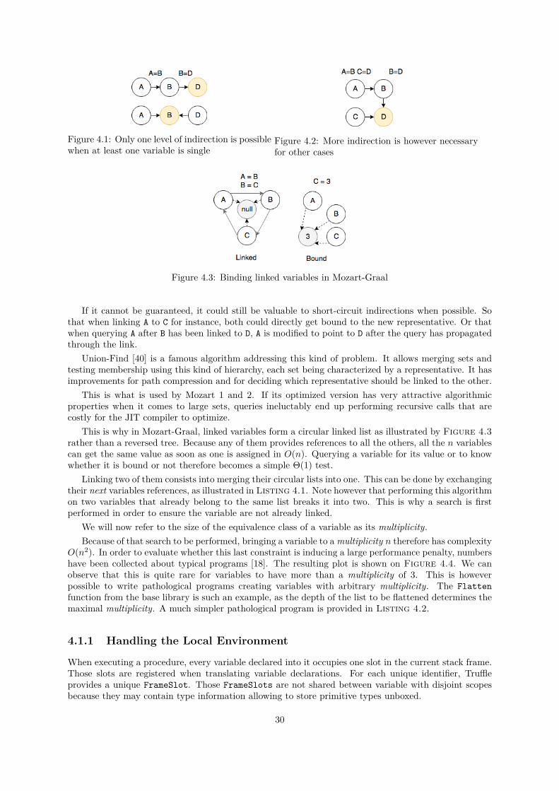
Figure 4.1: Only one level of indirection is possiblewhen at least one variable is single
Figure 4.2: More indirection is however necessaryfor other cases
Figure 4.3: Binding linked variables in Mozart-Graal
If it cannot be guaranteed, it could still be valuable to short-circuit indirections when possible. Sothat when linking A to C for instance, both could directly get bound to the new representative. Or thatwhen querying A after B has been linked to D, A is modified to point to D after the query has propagatedthrough the link.
Union-Find [40] is a famous algorithm addressing this kind of problem. It allows merging sets andtesting membership using this kind of hierarchy, each set being characterized by a representative. It hasimprovements for path compression and for deciding which representative should be linked to the other.
This is what is used by Mozart 1 and 2. If its optimized version has very attractive algorithmicproperties when it comes to large sets, queries ineluctably end up performing recursive calls that arecostly for the JIT compiler to optimize.
This is why in Mozart-Graal, linked variables form a circular linked list as illustrated by Figure 4.3rather than a reversed tree. Because any of them provides references to all the others, all the n variablescan get the same value as soon as one is assigned in O(n). Querying a variable for its value or to knowwhether it is bound or not therefore becomes a simple Θ(1) test.
Linking two of them consists into merging their circular lists into one. This can be done by exchangingtheir next variables references, as illustrated in Listing 4.1. Note however that performing this algorithmon two variables that already belong to the same list breaks it into two. This is why a search is firstperformed in order to ensure the variable are not already linked.
We will now refer to the size of the equivalence class of a variable as its multiplicity.Because of that search to be performed, bringing a variable to amultiplicity n therefore has complexity
O(n2). In order to evaluate whether this last constraint is inducing a large performance penalty, numbershave been collected about typical programs [18]. The resulting plot is shown on Figure 4.4. We canobserve that this is quite rare for variables to have more than a multiplicity of 3. This is howeverpossible to write pathological programs creating variables with arbitrary multiplicity. The Flattenfunction from the base library is such an example, as the depth of the list to be flattened determines themaximal multiplicity. A much simpler pathological program is provided in Listing 4.2.
4.1.1 Handling the Local Environment
When executing a procedure, every variable declared into it occupies one slot in the current stack frame.Those slots are registered when translating variable declarations. For each unique identifier, Truffleprovides a unique FrameSlot. Those FrameSlots are not shared between variable with disjoint scopesbecause they may contain type information allowing to store primitive types unboxed.
30
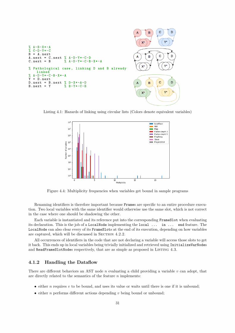
% A-B-X*-A% C-D-Y*-CB = A.nextA.next = C.next % A-D-Y*-C-DC.next = B % A-D-Y*-C-B-X*-A
% Pathological case , linking D and B alreadylinked
% A-D-Y*-C-B-X*-AY = D.nextD.next = B.next % D-X*-A-DB.next = Y % B-Y*-C-B
Listing 4.1: Hazards of linking using circular lists (Colors denote equivalent variables)
Figure 4.4: Multiplicity frequencies when variables get bound in sample programs
Renaming identifiers is therefore important because Frames are specific to an entire procedure execu-tion. Two local variables with the same identifier would otherwise use the same slot, which is not correctin the case where one should be shadowing the other.
Each variable is instantiated and its reference put into the corresponding FrameSlot when evaluatingits declaration. This is the job of a LocalNode implementing the local ... in ... end feature. TheLocalNode can also clear every of its FrameSlots at the end of its execution, depending on how variablesare captured, which will be discussed in Section 4.2.2.
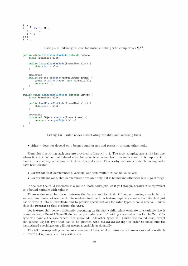
All occurrences of identifiers in the code that are not declaring a variable will access those slots to getit back. This ends up in local variables being trivially initialized and retrieved using InitializeVarNodesand ReadFrameSlotNodes respectively, that are as simple as proposed in Listing 4.3.
4.1.2 Handling the Dataflow
There are different behaviors an AST node n evaluating a child providing a variable v can adopt, thatare directly related to the semantics of the feature n implements:
• either n requires v to be bound, and uses its value or waits until there is one if it is unbound;• either n performs different actions depending v being bound or unbound;
31
A = _for I in 1..N do
B = _ inA = B
endA = 1
Listing 4.2: Pathological case for variable linking with complexity O(N2)
public class InitializeVarNode extends OzNode {final FrameSlot slot;
public InitializeVarNode(FrameSlot slot) {this.slot = slot;
}
@Overridepublic Object execute(VirtualFrame frame) {
frame.setObject(slot, new Variable());return unit;
}}
public class ReadFrameSlotNode extends OzNode {final FrameSlot slot;
public ReadFrameSlotNode(FrameSlot slot) {this.slot = slot;
}
@Overrideprotected Object execute(Frame frame) {
return frame.getObject(slot);}
}
Listing 4.3: Truffle nodes instantiating variables and accessing them
• either n does not depend on v being bound or not and passes it to some other node.
Examples illustrating each case are provided in Listing 4.4. The most complex case is the last one,where it is not defined beforehand what behavior is expected from the unification. It is important tohave a practical way of dealing with those different cases. This is why two kinds of dereferencing nodeshave been created:
• DerefNode that dereferences a variable, and thus waits if it has no value yet;• DerefIfBoundNode, that dereferences a variable only if it is bound and otherwise lets it go through.
In the case the child evaluates to a value v, both nodes just let it go through, because it is equivalentto a bound variable with value v.
Those nodes must be placed between the feature and its child. Of course, passing a variable or avalue around does not need such intermediate treatment. A feature requiring a value from its child justhas to wrap it into a DerefNode and to provide specializations for value types it could receive. This isthus the DerefNode that performs the Wait.
For features that behave differently depending on the fact a child might evaluate to a variable that isbound or not, a DerefIfBoundNode can be put in-between. Providing a specialization for the Variabletype will handle the case where it is unbound. All other types will handle the bound case, exceptthe generic Object type that has to be guarded with !isVariable(obj) in order to make sure theinstantiated specialization will not accept a variable accidentally.
The AST corresponding to the last statement of Listing 4.4 makes use of those nodes and is availablein Figure 4.5, along with its justification.
32
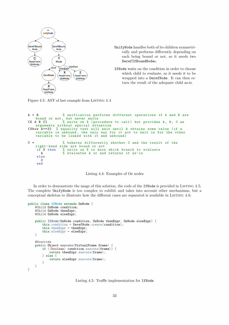
Figure 4.5: AST of last example from Listing 4.4
UnifyNode handles both of its children symmetri-cally and performs differently depending oneach being bound or not, so it needs twoDerefIfBoundNodes.
IfNode waits on the condition in order to choosewhich child to evaluate, so it needs it to bewrapped into a DerefNode. It can then re-turn the result of the adequate child as-is.
A = B % unification performs different operations if A and B arebound or not , but never waits
{X A B C} % waits on X ( procedure to call) but provides A, B, C asarguments without special attention
{Show A==3} % equality test will wait until A obtains some value (if avariable is unbound , the only way for it not to wait is for the othervariable to be linked with it and unbound )
C = % behaves differently whether C and the result of theright -hand side are bound or notif X then % waits on X to know which branch to evaluate
A % evaluates A or and returns it as -iselse
2end
Listing 4.4: Examples of Oz nodes
In order to demonstrate the usage of this solution, the code of the IfNode is provided in Listing 4.5.The complete UnifyNode is too complex to exhibit and takes into account other mechanisms, but aconceptual skeleton to illustrate how the different cases are separated is available in Listing 4.6.
public class IfNode extends OzNode {@Child OzNode condition;@Child OzNode thenExpr;@Child OzNode elseExpr;
public IfNode(OzNode condition, OzNode thenExpr, OzNode elseExpr) {this.condition = DerefNode.create(condition);this.thenExpr = thenExpr;this.elseExpr = elseExpr;
}
@Overridepublic Object execute(VirtualFrame frame) {
if ((boolean) condition.execute(frame)) {return thenExpr.execute(frame);
} else {return elseExpr.execute(frame);
}}
}
Listing 4.5: Truffle implementation for IfNode
33
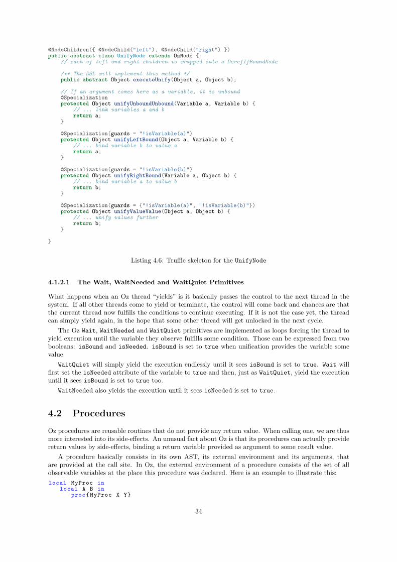
@NodeChildren({ @NodeChild("left"), @NodeChild("right") })public abstract class UnifyNode extends OzNode {
// each of left and right children is wrapped into a DerefIfBoundNode
/** The DSL will implement this method */public abstract Object executeUnify(Object a, Object b);
// If an argument comes here as a variable, it is unbound@Specializationprotected Object unifyUnboundUnbound(Variable a, Variable b) {
// ... link variables a and breturn a;
}
@Specialization(guards = "!isVariable(a)")protected Object unifyLeftBound(Object a, Variable b) {
// ... bind variable b to value areturn a;
}
@Specialization(guards = "!isVariable(b)")protected Object unifyRightBound(Variable a, Object b) {
// ... bind variable a to value breturn b;
}
@Specialization(guards = {"!isVariable(a)", "!isVariable(b)"})protected Object unifyValueValue(Object a, Object b) {
// ... unify values furtherreturn b;
}
}
Listing 4.6: Truffle skeleton for the UnifyNode
4.1.2.1 The Wait, WaitNeeded and WaitQuiet Primitives
What happens when an Oz thread “yields” is it basically passes the control to the next thread in thesystem. If all other threads come to yield or terminate, the control will come back and chances are thatthe current thread now fulfills the conditions to continue executing. If it is not the case yet, the threadcan simply yield again, in the hope that some other thread will get unlocked in the next cycle.
The Oz Wait, WaitNeeded and WaitQuiet primitives are implemented as loops forcing the thread toyield execution until the variable they observe fulfills some condition. Those can be expressed from twobooleans: isBound and isNeeded. isBound is set to true when unification provides the variable somevalue.
WaitQuiet will simply yield the execution endlessly until it sees isBound is set to true. Wait willfirst set the isNeeded attribute of the variable to true and then, just as WaitQuiet, yield the executionuntil it sees isBound is set to true too.
WaitNeeded also yields the execution until it sees isNeeded is set to true.
4.2 Procedures
Oz procedures are reusable routines that do not provide any return value. When calling one, we are thusmore interested into its side-effects. An unusual fact about Oz is that its procedures can actually providereturn values by side-effects, binding a return variable provided as argument to some result value.
A procedure basically consists in its own AST, its external environment and its arguments, thatare provided at the call site. In Oz, the external environment of a procedure consists of the set of allobservable variables at the place this procedure was declared. Here is an example to illustrate this:local MyProc in
local A B inproc{ MyProc X Y}
34
{ Browse A#B#X#Y} % Use both external and local environmentsendB = 2A = 1
end% A and B cannot be accessed here , but the procedure conserves them% into its external environment .{ MyProc 3 4} % the call site => Browses 1#2#3#4
end
We can see that A and B are still accessible by the body of the procedure, even though in practice,this code gets called outside of their scope.
4.2.1 Handling the Arguments
Truffle’s frame contains the call arguments as an Object[] array. In Mozart-Graal, its elements aresimply transfered from this array to the local slots at the very beginning of the procedure execution.
This is very convenient because they can then be handled as other local variables in the translationand when performing optimizations, therefore avoiding feature duplication. It also provides a place tostore new arguments in the array while computing them in Section 5.1.1. This is thus not wastedspace.
As a side note, the first slot of the arguments array will be reserved to the external environment.Because it is specific to procedure instances, it cannot be linked to AST directly.
4.2.2 Implementing the External Environment
The Translator maintains a hierarchy of environments while translating the AST generated by thestatic analyzer. This means it has access to all the information about the variables reachable by thestatements it translates, and therefore knows whether a variable was declared in the current procedureor not. In the case a variable cannot be found locally, the Translator is able to find the environment ithas been declared in.
At runtime, environments are composed of Truffle Frames. If the classical VirtualFrame that is passedrecursively between execute methods cannot be stored, the MaterializedFrame can be instantiated andpassed around as any Java object. This is thus the perfect candidate for storing external environments.
There is however some freedom as to how to organize those. A first proposition consists in creatinga linked list of frames to access the environments the parent procedures have been declared in. Both thedepth in the list and the FrameSlot to reach any variable are known to the Translator, so this can beefficiently implemented.
The second and retained fashion is for each procedure to have a single MaterializedFrame thatregroups just the required part of the external environment. It will be referred to as “variable selection”in the rest of this dissertation. When a procedure declaration is evaluated, the new frame is createdcontaining all the variables it could need for later calls. The Translator must therefore instantiatenodes propagating interesting variables from procedure to procedure. Here is an example of the problemit must solve:proc{X}
A=1 B Y inproc{Y} % Along with this procedure , a frame containing A and B must be
created (A must be propagated to Z’s declaration )C=3 D=4 Z
inB=2proc{Z E F} % Along with this procedure , a frame containing A and C
must be created{ Browse [A C E]} % Browses "[1 3 5]"
end{Z 5 6}
end{Y}
end
35
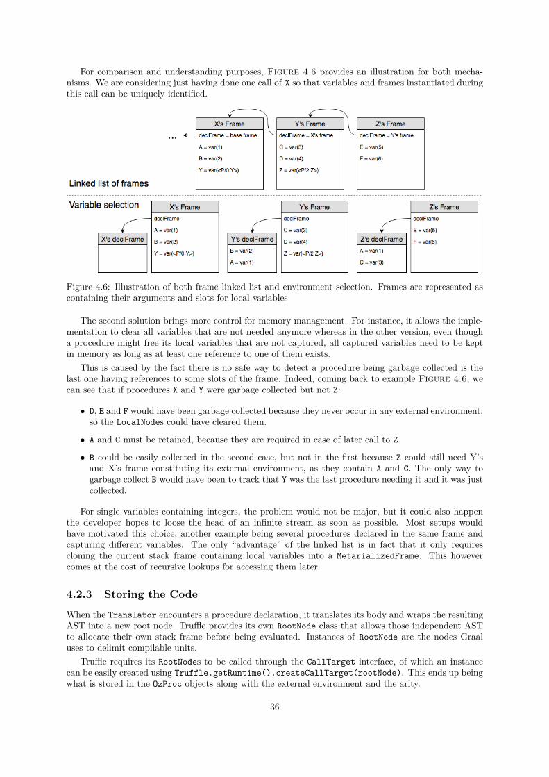
For comparison and understanding purposes, Figure 4.6 provides an illustration for both mecha-nisms. We are considering just having done one call of X so that variables and frames instantiated duringthis call can be uniquely identified.
Figure 4.6: Illustration of both frame linked list and environment selection. Frames are represented ascontaining their arguments and slots for local variables
The second solution brings more control for memory management. For instance, it allows the imple-mentation to clear all variables that are not needed anymore whereas in the other version, even thougha procedure might free its local variables that are not captured, all captured variables need to be keptin memory as long as at least one reference to one of them exists.
This is caused by the fact there is no safe way to detect a procedure being garbage collected is thelast one having references to some slots of the frame. Indeed, coming back to example Figure 4.6, wecan see that if procedures X and Y were garbage collected but not Z:
• D, E and F would have been garbage collected because they never occur in any external environment,so the LocalNodes could have cleared them.
• A and C must be retained, because they are required in case of later call to Z.
• B could be easily collected in the second case, but not in the first because Z could still need Y’sand X’s frame constituting its external environment, as they contain A and C. The only way togarbage collect B would have been to track that Y was the last procedure needing it and it was justcollected.
For single variables containing integers, the problem would not be major, but it could also happenthe developer hopes to loose the head of an infinite stream as soon as possible. Most setups wouldhave motivated this choice, another example being several procedures declared in the same frame andcapturing different variables. The only “advantage” of the linked list is in fact that it only requirescloning the current stack frame containing local variables into a MetarializedFrame. This howevercomes at the cost of recursive lookups for accessing them later.
4.2.3 Storing the Code
When the Translator encounters a procedure declaration, it translates its body and wraps the resultingAST into a new root node. Truffle provides its own RootNode class that allows those independent ASTto allocate their own stack frame before being evaluated. Instances of RootNode are the nodes Graaluses to delimit compilable units.
Truffle requires its RootNodes to be called through the CallTarget interface, of which an instancecan be easily created using Truffle.getRuntime().createCallTarget(rootNode). This ends up beingwhat is stored in the OzProc objects along with the external environment and the arity.
36
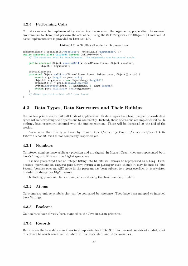
4.2.4 Performing Calls
Oz calls can now be implemented by evaluating the receiver, the arguments, prepending the externalenvironment to them, and perform the actual call using the CallTarget’s call(Object[]) method. Abasic implementation is provided in Listing 4.7.
Listing 4.7: A Truffle call node for Oz procedures
@NodeChildren({ @NodeChild("receiver"), @NodeChild("arguments") })public abstract class CallNode extends CallableNode {
// The receiver must be dereferenced, the arguments can be passed as-is.
public abstract Object executeCall(VirtualFrame frame, Object receiver,Object[] arguments);
@Specializationprotected Object callProc(VirtualFrame frame, OzProc proc, Object[] args) {
assert args.length == proc.arity;Object[] arguments = new Object[args.length+1];arguments[0] = proc.declarationFrame;System.arraycopy(args, 0, arguments, 1, args.length);return proc.callTarget.call(arguments);
}// Other specializations will come later
}
4.3 Data Types, Data Structures and Their Builtins
Oz has few primitives to build all kinds of applications. Its data types have been mapped towards Javatypes without exposing their operations to Oz directly. Instead, those operations are implemented as Ozbuiltins, base procedures shipped with the implementation. Those will be discussed at the end of thesection.
Please note that the type hierarchy from https://mozart.github.io/mozart-v1/doc-1.4.0/tutorial/node3.html is not completely respected yet.
4.3.1 Numbers
Oz integer numbers have arbitrary precision and are signed. In Mozart-Graal, they are represented bothJava’s long primitive and the BigInteger class.
It is not guaranteed that an integer fitting into 64 bits will always be represented as a long. First,because operations on BigIntegers always return a BigInteger even though it may fit into 64 bits.Second, because once an AST node in the program has been subject to a long overflow, it is rewrittenin order to always use BigIntegers.
Oz floating points numbers are implemented using the Java double primitive.
4.3.2 Atoms
Oz atoms are unique symbols that can be compared by reference. They have been mapped to internedJava Strings.
4.3.3 Booleans
Oz booleans have directly been mapped to the Java boolean primitive.
4.3.4 Records
Records are the base data structures to group variables in Oz [33]. Each record consists of a label, a setof features to which contained variables will be associated, and those variables.
37
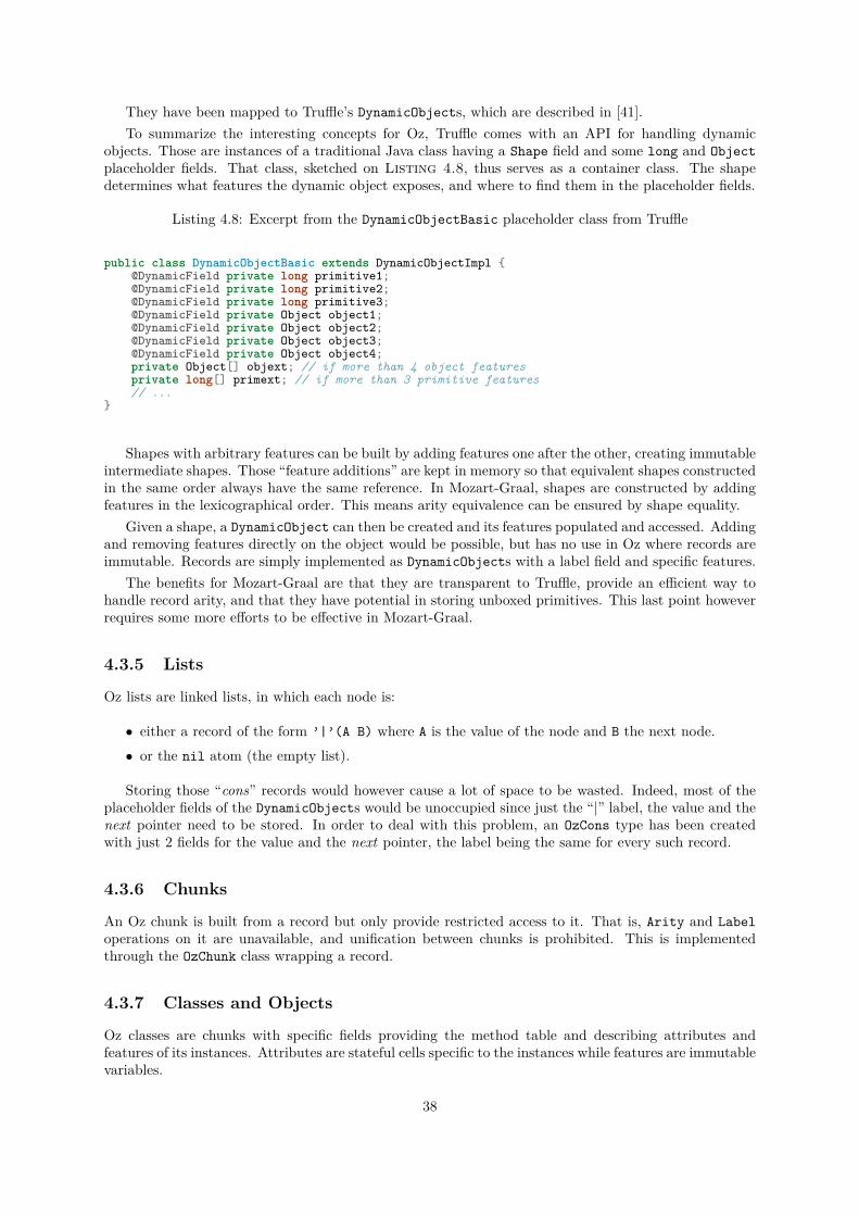
They have been mapped to Truffle’s DynamicObjects, which are described in [41].To summarize the interesting concepts for Oz, Truffle comes with an API for handling dynamic
objects. Those are instances of a traditional Java class having a Shape field and some long and Objectplaceholder fields. That class, sketched on Listing 4.8, thus serves as a container class. The shapedetermines what features the dynamic object exposes, and where to find them in the placeholder fields.
Listing 4.8: Excerpt from the DynamicObjectBasic placeholder class from Truffle
public class DynamicObjectBasic extends DynamicObjectImpl {@DynamicField private long primitive1;@DynamicField private long primitive2;@DynamicField private long primitive3;@DynamicField private Object object1;@DynamicField private Object object2;@DynamicField private Object object3;@DynamicField private Object object4;private Object[] objext; // if more than 4 object featuresprivate long[] primext; // if more than 3 primitive features// ...
}
Shapes with arbitrary features can be built by adding features one after the other, creating immutableintermediate shapes. Those “feature additions” are kept in memory so that equivalent shapes constructedin the same order always have the same reference. In Mozart-Graal, shapes are constructed by addingfeatures in the lexicographical order. This means arity equivalence can be ensured by shape equality.
Given a shape, a DynamicObject can then be created and its features populated and accessed. Addingand removing features directly on the object would be possible, but has no use in Oz where records areimmutable. Records are simply implemented as DynamicObjects with a label field and specific features.
The benefits for Mozart-Graal are that they are transparent to Truffle, provide an efficient way tohandle record arity, and that they have potential in storing unboxed primitives. This last point howeverrequires some more efforts to be effective in Mozart-Graal.
4.3.5 Lists
Oz lists are linked lists, in which each node is:
• either a record of the form ’|’(A B) where A is the value of the node and B the next node.• or the nil atom (the empty list).
Storing those “cons” records would however cause a lot of space to be wasted. Indeed, most of theplaceholder fields of the DynamicObjects would be unoccupied since just the “|” label, the value and thenext pointer need to be stored. In order to deal with this problem, an OzCons type has been createdwith just 2 fields for the value and the next pointer, the label being the same for every such record.
4.3.6 Chunks
An Oz chunk is built from a record but only provide restricted access to it. That is, Arity and Labeloperations on it are unavailable, and unification between chunks is prohibited. This is implementedthrough the OzChunk class wrapping a record.
4.3.7 Classes and Objects
Oz classes are chunks with specific fields providing the method table and describing attributes andfeatures of its instances. Attributes are stateful cells specific to the instances while features are immutablevariables.
38
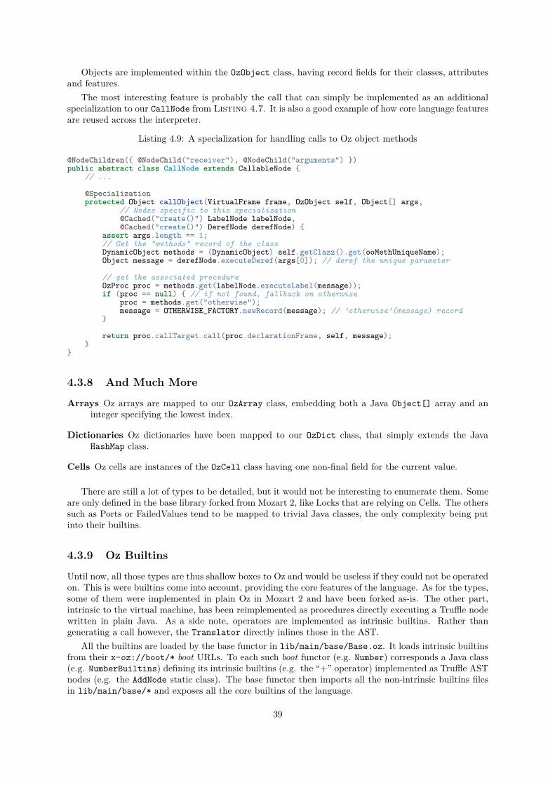
Objects are implemented within the OzObject class, having record fields for their classes, attributesand features.
The most interesting feature is probably the call that can simply be implemented as an additionalspecialization to our CallNode from Listing 4.7. It is also a good example of how core language featuresare reused across the interpreter.
Listing 4.9: A specialization for handling calls to Oz object methods
@NodeChildren({ @NodeChild("receiver"), @NodeChild("arguments") })public abstract class CallNode extends CallableNode {
// ...
@Specializationprotected Object callObject(VirtualFrame frame, OzObject self, Object[] args,
// Nodes specific to this specialization@Cached("create()") LabelNode labelNode,@Cached("create()") DerefNode derefNode) {
assert args.length == 1;// Get the "methods" record of the classDynamicObject methods = (DynamicObject) self.getClazz().get(ooMethUniqueName);Object message = derefNode.executeDeref(args[0]); // deref the unique parameter
// get the associated procedureOzProc proc = methods.get(labelNode.executeLabel(message));if (proc == null) { // if not found, fallback on otherwise
proc = methods.get("otherwise");message = OTHERWISE_FACTORY.newRecord(message); // ’otherwise’(message) record
}
return proc.callTarget.call(proc.declarationFrame, self, message);}
}
4.3.8 And Much More
Arrays Oz arrays are mapped to our OzArray class, embedding both a Java Object[] array and aninteger specifying the lowest index.
Dictionaries Oz dictionaries have been mapped to our OzDict class, that simply extends the JavaHashMap class.
Cells Oz cells are instances of the OzCell class having one non-final field for the current value.
There are still a lot of types to be detailed, but it would not be interesting to enumerate them. Someare only defined in the base library forked from Mozart 2, like Locks that are relying on Cells. The otherssuch as Ports or FailedValues tend to be mapped to trivial Java classes, the only complexity being putinto their builtins.
4.3.9 Oz Builtins
Until now, all those types are thus shallow boxes to Oz and would be useless if they could not be operatedon. This is were builtins come into account, providing the core features of the language. As for the types,some of them were implemented in plain Oz in Mozart 2 and have been forked as-is. The other part,intrinsic to the virtual machine, has been reimplemented as procedures directly executing a Truffle nodewritten in plain Java. As a side note, operators are implemented as intrinsic builtins. Rather thangenerating a call however, the Translator directly inlines those in the AST.
All the builtins are loaded by the base functor in lib/main/base/Base.oz. It loads intrinsic builtinsfrom their x-oz://boot/* boot URLs. To each such boot functor (e.g. Number) corresponds a Java class(e.g. NumberBuiltins) defining its intrinsic builtins (e.g. the “+” operator) implemented as Truffle ASTnodes (e.g. the AddNode static class). The base functor then imports all the non-intrinsic builtins filesin lib/main/base/* and exposes all the core builtins of the language.
39
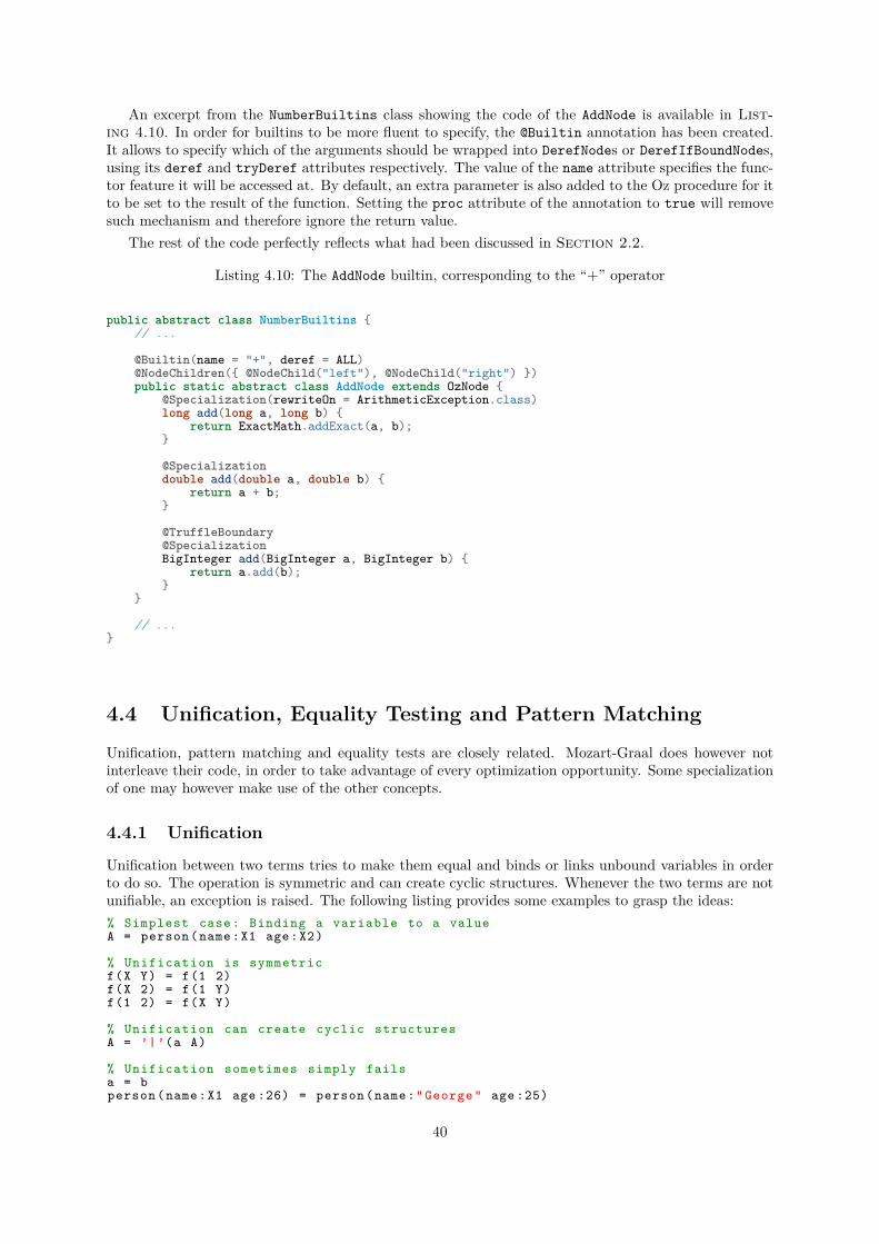
An excerpt from the NumberBuiltins class showing the code of the AddNode is available in List-ing 4.10. In order for builtins to be more fluent to specify, the @Builtin annotation has been created.It allows to specify which of the arguments should be wrapped into DerefNodes or DerefIfBoundNodes,using its deref and tryDeref attributes respectively. The value of the name attribute specifies the func-tor feature it will be accessed at. By default, an extra parameter is also added to the Oz procedure for itto be set to the result of the function. Setting the proc attribute of the annotation to true will removesuch mechanism and therefore ignore the return value.
The rest of the code perfectly reflects what had been discussed in Section 2.2.
Listing 4.10: The AddNode builtin, corresponding to the “+” operator
public abstract class NumberBuiltins {// ...
@Builtin(name = "+", deref = ALL)@NodeChildren({ @NodeChild("left"), @NodeChild("right") })public static abstract class AddNode extends OzNode {
@Specialization(rewriteOn = ArithmeticException.class)long add(long a, long b) {
return ExactMath.addExact(a, b);}
@Specializationdouble add(double a, double b) {
return a + b;}
@TruffleBoundary@SpecializationBigInteger add(BigInteger a, BigInteger b) {
return a.add(b);}
}
// ...}
4.4 Unification, Equality Testing and Pattern Matching
Unification, pattern matching and equality tests are closely related. Mozart-Graal does however notinterleave their code, in order to take advantage of every optimization opportunity. Some specializationof one may however make use of the other concepts.
4.4.1 Unification
Unification between two terms tries to make them equal and binds or links unbound variables in orderto do so. The operation is symmetric and can create cyclic structures. Whenever the two terms are notunifiable, an exception is raised. The following listing provides some examples to grasp the ideas:% Simplest case: Binding a variable to a valueA = person (name:X1 age:X2)
% Unification is symmetricf(X Y) = f(1 2)f(X 2) = f(1 Y)f(1 2) = f(X Y)
% Unification can create cyclic structuresA = ’|’(a A)
% Unification sometimes simply failsa = bperson (name:X1 age :26) = person (name:" George " age :25)
40
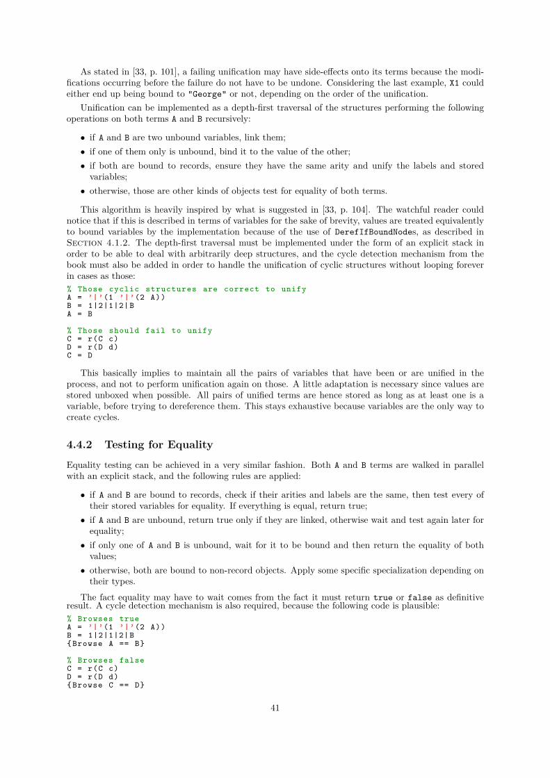
As stated in [33, p. 101], a failing unification may have side-effects onto its terms because the modi-fications occurring before the failure do not have to be undone. Considering the last example, X1 couldeither end up being bound to "George" or not, depending on the order of the unification.
Unification can be implemented as a depth-first traversal of the structures performing the followingoperations on both terms A and B recursively:
• if A and B are two unbound variables, link them;• if one of them only is unbound, bind it to the value of the other;• if both are bound to records, ensure they have the same arity and unify the labels and storedvariables;
• otherwise, those are other kinds of objects test for equality of both terms.
This algorithm is heavily inspired by what is suggested in [33, p. 104]. The watchful reader couldnotice that if this is described in terms of variables for the sake of brevity, values are treated equivalentlyto bound variables by the implementation because of the use of DerefIfBoundNodes, as described inSection 4.1.2. The depth-first traversal must be implemented under the form of an explicit stack inorder to be able to deal with arbitrarily deep structures, and the cycle detection mechanism from thebook must also be added in order to handle the unification of cyclic structures without looping foreverin cases as those:% Those cyclic structures are correct to unifyA = ’|’(1 ’|’(2 A))B = 1|2|1|2| BA = B
% Those should fail to unifyC = r(C c)D = r(D d)C = D
This basically implies to maintain all the pairs of variables that have been or are unified in theprocess, and not to perform unification again on those. A little adaptation is necessary since values arestored unboxed when possible. All pairs of unified terms are hence stored as long as at least one is avariable, before trying to dereference them. This stays exhaustive because variables are the only way tocreate cycles.
4.4.2 Testing for Equality
Equality testing can be achieved in a very similar fashion. Both A and B terms are walked in parallelwith an explicit stack, and the following rules are applied:
• if A and B are bound to records, check if their arities and labels are the same, then test every oftheir stored variables for equality. If everything is equal, return true;
• if A and B are unbound, return true only if they are linked, otherwise wait and test again later forequality;
• if only one of A and B is unbound, wait for it to be bound and then return the equality of bothvalues;
• otherwise, both are bound to non-record objects. Apply some specific specialization depending ontheir types.
The fact equality may have to wait comes from the fact it must return true or false as definitiveresult. A cycle detection mechanism is also required, because the following code is plausible:% Browses trueA = ’|’(1 ’|’(2 A))B = 1|2|1|2| B{ Browse A == B}
% Browses falseC = r(C c)D = r(D d){ Browse C == D}
41
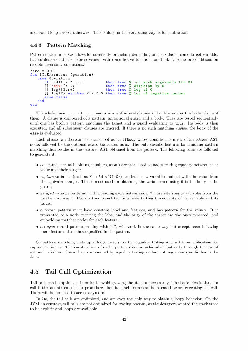
and would loop forever otherwise. This is done in the very same way as for unification.
4.4.3 Pattern Matching
Pattern matching in Oz allows for succinctly branching depending on the value of some target variable.Let us demonstrate its expressiveness with some fictive function for checking some preconditions onrecords describing operations:Zero = 0.0fun { IsErroneous Operation }
case Operationof add(X Y Z ...) then true % too much arguments (>= 3)[] ’div ’(X 0) then true % division by 0[] log (! Zero) then true % log of 0[] log(Y) andthen Y < 0.0 then true % log of negative numberelse false
endend
The whole case ... of ... end is made of several clauses and only executes the body of one ofthem. A clause is composed of a pattern, an optional guard and a body. They are tested sequentiallyuntil one has both a pattern matching the target and a guard evaluating to true. Its body is thenexecuted, and all subsequent clauses are ignored. If there is no such matching clause, the body of theelse is evaluated.
Each clause can therefore be translated as an IfNode whose condition is made of a matcher ASTnode, followed by the optional guard translated as-is. The only specific features for handling patternmatching thus resides in the matcher AST obtained from the pattern. The following rules are followedto generate it:
• constants such as booleans, numbers, atoms are translated as nodes testing equality between theirvalue and their target;
• capture variables (such as X in ’div’(X 0)) are fresh new variables unified with the value fromthe equivalent target. This is most used for obtaining the variable and using it in the body or theguard;
• escaped variable patterns, with a leading exclamation mark “!”, are referring to variables from thelocal environment. Each is thus translated to a node testing the equality of its variable and itstarget;
• a record pattern must have constant label and features, and has pattern for the values. It istranslated to a node ensuring the label and the arity of the target are the ones expected, andembedding matcher nodes for each feature;
• an open record pattern, ending with “...”, will work in the same way but accept records havingmore features than those specified in the pattern.
So pattern matching ends up relying mostly on the equality testing and a bit on unification forcapture variables. The construction of cyclic patterns is also achievable, but only through the use ofescaped variables. Since they are handled by equality testing nodes, nothing more specific has to bedone.
4.5 Tail Call Optimization
Tail calls can be optimized in order to avoid growing the stack unnecessarily. The basic idea is that if acall is the last statement of a procedure, then its stack frame can be released before executing the call.There will be no need to access anymore.
In Oz, the tail calls are optimized, and are even the only way to obtain a loopy behavior. On theJVM, in contrast, tail calls are not optimized for tracing reasons, as the designers wanted the stack traceto be explicit and loops are available.
42
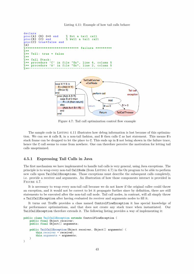
Listing 4.11: Example of how tail calls behave
declareproc{A} {B} 0=0 end % Not a tail callproc{B} {C} end % Well a tail callproc{C} true=false end{A}% ***************************** failure *********%**%** Tell: true = false%**%** Call Stack:%** procedure ’C’ in file "Oz", line 4, column 5%** procedure ’A’ in file "Oz", line 2, column 5%**---------------------------------------------
Figure 4.7: Tail call optimization control flow example
The sample code in Listing 4.11 illustrates how debug information is lost because of this optimiza-tion. We can see A calls B, in a non-tail fashion, and B then calls C as last statement. This means B’sstack frame can be dropped to let the place to C. This ends up in B not being shown in the failure trace,hence the C call seems to come from nowhere. One can therefore perceive the motivation for letting tailcalls unoptimized.
4.5.1 Expressing Tail Calls in Java
The first mechanism we have implemented to handle tail calls is very general, using Java exceptions. Theprinciple is to wrap every non-tail CallNode (from Listing 4.7) in the Oz program to be able to performnew calls upon TailCallExceptions. Those exceptions must describe the subsequent calls completely,i.e. provide a receiver and arguments. An illustration of how those components interact is provided inFigure 4.7.
It is necessary to wrap every non-tail call because we do not know if the original callee could throwan exception, and it would not be correct to let it propagate further since by definition, there are stillstatements to be executed after the non-tail call node. Tail call nodes, in contrast, will all simply throwa TailCallException after having evaluated its receiver and arguments nodes to fill it.
It turns out Truffle provides a class named ControlFlowException it has special knowledge offor performance optimizations, and that does not create any stack trace when instantiated. OurTailCallException therefore extends it. The following listing provides a way of implementing it:
public class TailCallException extends ControlFlowException {public final Object receiver;public final Object[] arguments;
public TailCallException(Object receiver, Object[] arguments) {this.receiver = receiver;this.arguments = arguments;
}}
43
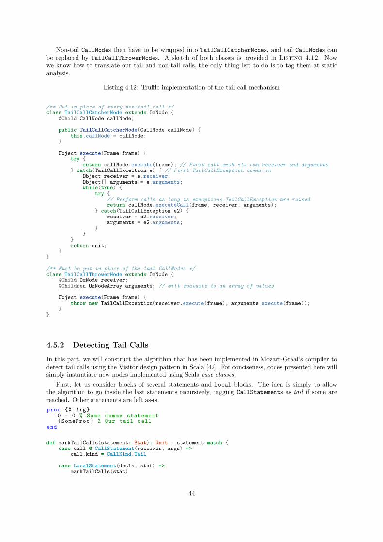
Non-tail CallNodes then have to be wrapped into TailCallCatcherNodes, and tail CallNodes canbe replaced by TailCallThrowerNodes. A sketch of both classes is provided in Listing 4.12. Nowwe know how to translate our tail and non-tail calls, the only thing left to do is to tag them at staticanalysis.
Listing 4.12: Truffle implementation of the tail call mechanism
/** Put in place of every non-tail call */class TailCallCatcherNode extends OzNode {
@Child CallNode callNode;
public TailCallCatcherNode(CallNode callNode) {this.callNode = callNode;
}
Object execute(Frame frame) {try {
return callNode.execute(frame); // First call with its own receiver and arguments} catch(TailCallException e) { // First TailCallException comes in
Object receiver = e.receiver;Object[] arguments = e.arguments;while(true) {
try {// Perform calls as long as execptions TailCallException are raisedreturn callNode.executeCall(frame, receiver, arguments);
} catch(TailCallException e2) {receiver = e2.receiver;arguments = e2.arguments;
}}
}return unit;
}}
/** Must be put in place of the tail CallNodes */class TailCallThrowerNode extends OzNode {
@Child OzNode receiver;@Children OzNodeArray arguments; // will evaluate to an array of values
Object execute(Frame frame) {throw new TailCallException(receiver.execute(frame), arguments.execute(frame));
}}
4.5.2 Detecting Tail Calls
In this part, we will construct the algorithm that has been implemented in Mozart-Graal’s compiler todetect tail calls using the Visitor design pattern in Scala [42]. For conciseness, codes presented here willsimply instantiate new nodes implemented using Scala case classes.
First, let us consider blocks of several statements and local blocks. The idea is simply to allowthe algorithm to go inside the last statements recursively, tagging CallStatements as tail if some arereached. Other statements are left as-is.proc {X Arg}
0 = 0 % Some dummy statement{ SomeProc } % Our tail call
end
def markTailCalls(statement: Stat): Unit = statement match {case call @ CallStatement(receiver, args) =>
call.kind = CallKind.Tail
case LocalStatement(decls, stat) =>markTailCalls(stat)
44
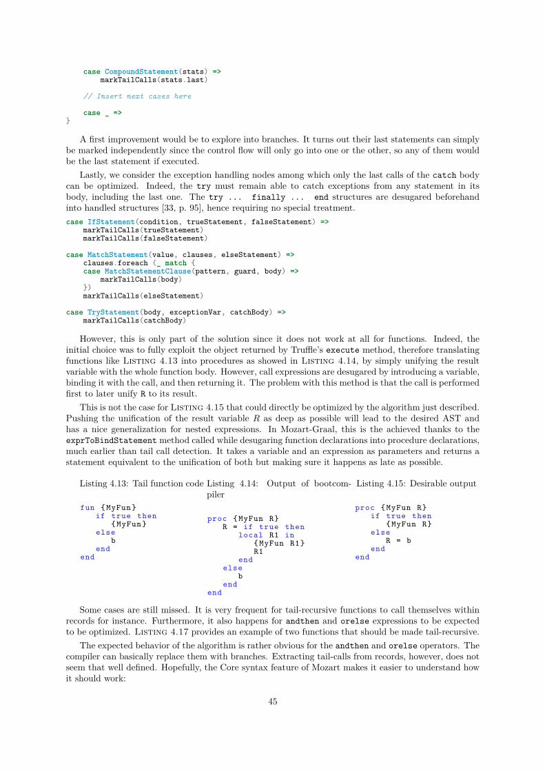
case CompoundStatement(stats) =>markTailCalls(stats.last)
// Insert next cases here
case _ =>}
A first improvement would be to explore into branches. It turns out their last statements can simplybe marked independently since the control flow will only go into one or the other, so any of them wouldbe the last statement if executed.
Lastly, we consider the exception handling nodes among which only the last calls of the catch bodycan be optimized. Indeed, the try must remain able to catch exceptions from any statement in itsbody, including the last one. The try ... finally ... end structures are desugared beforehandinto handled structures [33, p. 95], hence requiring no special treatment.case IfStatement(condition, trueStatement, falseStatement) =>
markTailCalls(trueStatement)markTailCalls(falseStatement)
case MatchStatement(value, clauses, elseStatement) =>clauses.foreach (_ match {case MatchStatementClause(pattern, guard, body) =>
markTailCalls(body)})markTailCalls(elseStatement)
case TryStatement(body, exceptionVar, catchBody) =>markTailCalls(catchBody)
However, this is only part of the solution since it does not work at all for functions. Indeed, theinitial choice was to fully exploit the object returned by Truffle’s execute method, therefore translatingfunctions like Listing 4.13 into procedures as showed in Listing 4.14, by simply unifying the resultvariable with the whole function body. However, call expressions are desugared by introducing a variable,binding it with the call, and then returning it. The problem with this method is that the call is performedfirst to later unify R to its result.
This is not the case for Listing 4.15 that could directly be optimized by the algorithm just described.Pushing the unification of the result variable R as deep as possible will lead to the desired AST andhas a nice generalization for nested expressions. In Mozart-Graal, this is the achieved thanks to theexprToBindStatement method called while desugaring function declarations into procedure declarations,much earlier than tail call detection. It takes a variable and an expression as parameters and returns astatement equivalent to the unification of both but making sure it happens as late as possible.
Listing 4.13: Tail function code
fun {MyFun}if true then
{MyFun}else
bend
end
Listing 4.14: Output of bootcom-piler
proc {MyFun R}R = if true then
local R1 in{MyFun R1}R1
endelse
bend
end
Listing 4.15: Desirable output
proc {MyFun R}if true then
{MyFun R}else
R = bend
end
Some cases are still missed. It is very frequent for tail-recursive functions to call themselves withinrecords for instance. Furthermore, it also happens for andthen and orelse expressions to be expectedto be optimized. Listing 4.17 provides an example of two functions that should be made tail-recursive.
The expected behavior of the algorithm is rather obvious for the andthen and orelse operators. Thecompiler can basically replace them with branches. Extracting tail-calls from records, however, does notseem that well defined. Hopefully, the Core syntax feature of Mozart makes it easier to understand howit should work:
45
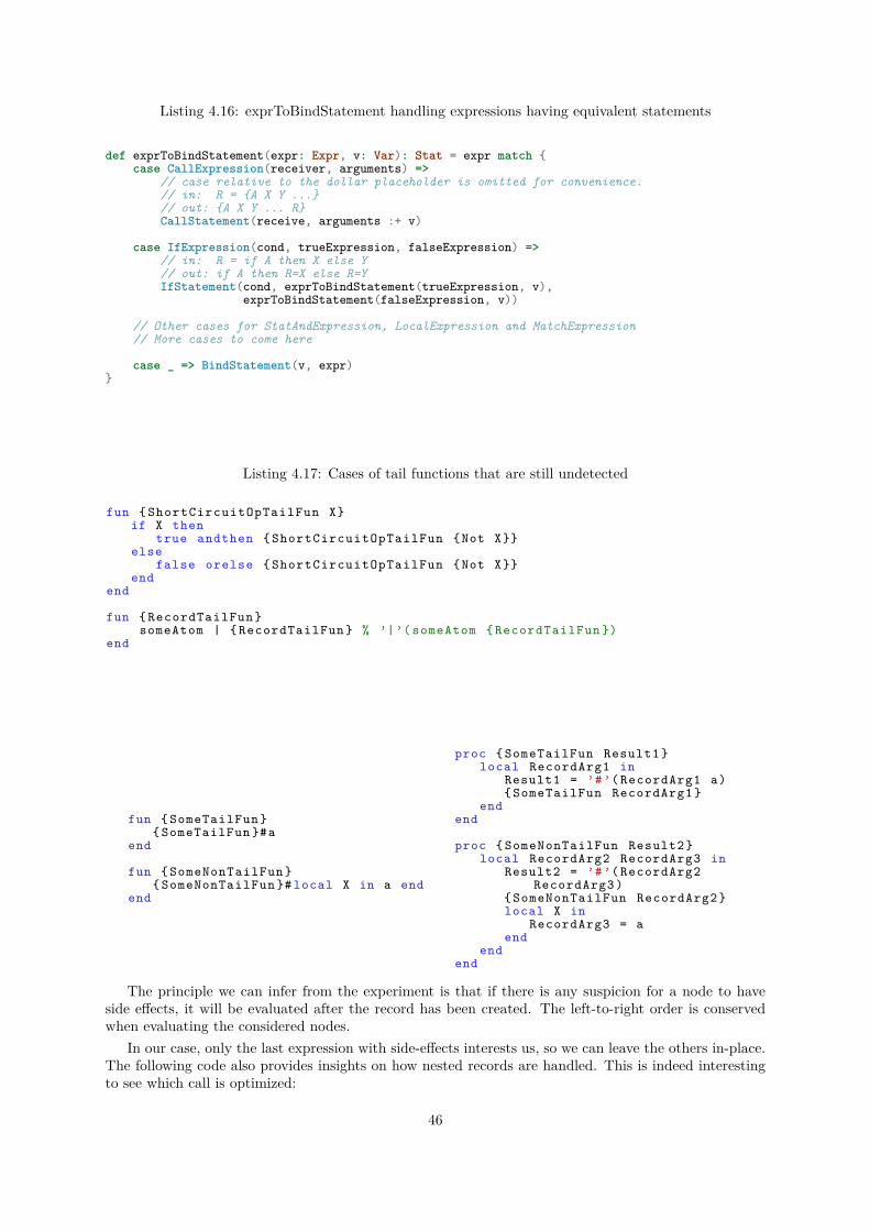
Listing 4.16: exprToBindStatement handling expressions having equivalent statements
def exprToBindStatement(expr: Expr, v: Var): Stat = expr match {case CallExpression(receiver, arguments) =>
// case relative to the dollar placeholder is omitted for convenience.// in: R = {A X Y ...}// out: {A X Y ... R}CallStatement(receive, arguments :+ v)
case IfExpression(cond, trueExpression, falseExpression) =>// in: R = if A then X else Y// out: if A then R=X else R=YIfStatement(cond, exprToBindStatement(trueExpression, v),
exprToBindStatement(falseExpression, v))
// Other cases for StatAndExpression, LocalExpression and MatchExpression// More cases to come here
case _ => BindStatement(v, expr)}
Listing 4.17: Cases of tail functions that are still undetected
fun { ShortCircuitOpTailFun X}if X then
true andthen { ShortCircuitOpTailFun {Not X}}else
false orelse { ShortCircuitOpTailFun {Not X}}end
end
fun { RecordTailFun }someAtom | { RecordTailFun } % ’|’( someAtom { RecordTailFun })
end
fun { SomeTailFun }{ SomeTailFun }#a
end
fun { SomeNonTailFun }{ SomeNonTailFun }# local X in a end
end
proc { SomeTailFun Result1 }local RecordArg1 in
Result1 = ’#’( RecordArg1 a){ SomeTailFun RecordArg1 }
endend
proc { SomeNonTailFun Result2 }local RecordArg2 RecordArg3 in
Result2 = ’#’( RecordArg2RecordArg3 )
{ SomeNonTailFun RecordArg2 }local X in
RecordArg3 = aend
endend
The principle we can infer from the experiment is that if there is any suspicion for a node to haveside effects, it will be evaluated after the record has been created. The left-to-right order is conservedwhen evaluating the considered nodes.
In our case, only the last expression with side-effects interests us, so we can leave the others in-place.The following code also provides insights on how nested records are handled. This is indeed interestingto see which call is optimized:
46
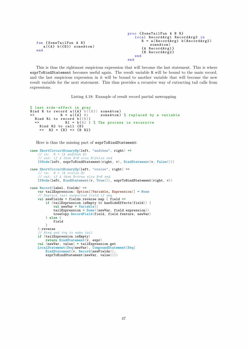
fun { SomeTailFun A B}a({A} b({B}) someAtom )
end
proc { SomeTailFun A B R}local RecordArg1 RecordArg2 in
R = a( RecordArg1 b( RecordArg2 )someAtom )
{A RecordArg1 }{B RecordArg2 }
endend
This is thus the rightmost suspicious expression that will become the last statement. This is whereexprToBindStatement becomes useful again. The result variable R will be bound to the main record,and the last suspicious expression in it will be bound to another variable that will become the newresult variable for the next statement. This thus provides a recursive way of extracting tail calls fromexpressions.
Listing 4.18: Example of result record partial unwrapping
% last side - effect in grayBind R to record a({A} b({B}) someAtom )=> R = a({A} R1 someAtom ) % replaced by a variable
Bind R1 to record b({B})=> R1 = b(R2 ) % The process is recursive
Bind R2 to call {B}=> R2 = {B} => {B R2}
Here is thus the missing part of exprToBindStatement:
case ShortCircuitBinaryOp(left, "andthen", right) =>// in: R = (A andthen B)// out: if A then R=B else R=false endIfNode(left, exprToBindStatement(right, v), BindStatement(v, False()))
case ShortCircuitBinaryOp(left, "orelse", right) =>// in: R = (A orelse B)// out: if A then R=true else R=B endIfNode(left, BindStatement(v, True()), exprToBindStatement(right, v))
case Record(label, fields) =>var tailExpression: Option[(Variable, Expression)] = None// Replace last suspected field if anyval newFields = fields.reverse.map { field =>
if (tailExpression.isEmpty && hasSideEffects(field)) {val newVar = Variable()tailExpression = Some((newVar, field.expression))treeCopy.RecordField(field, field.feature, newVar)
} else {field
}}.reverse// Bind and try to make tailif (tailExpression.isEmpty)
return BindStatement(v, expr)val (newVar, value) = tailExpression.getLocalStatement(Seq(newVar), CompoundStatement(Seq(
BindStatement(v, Record(newFields)),exprToBindStatement(newVar, value))))
47

48
Chapter 5
Specific Optimizations
In the previous chapter, we have mapped Oz concepts to Truffle without paying much attention toperformance. We will here propose several specific optimizations for increasing performance and memoryefficiency.
The first part will require additions the static analysis to avoid variables, optimize their retentionand optimize self tail calls.
By contrast, the second part only relies on the Truffle API to help Graal perform inlining and controlflow optimization as soon as possible. We also make use of self-optimizing AST interpreters principlesto propose more efficient mechanisms for unification and equality tests.
5.1 Static Optimizations
In this section, add information at static analysis to perform some optimizations. We first particularizethe mechanism for tail calls to self tail calls. We then see how it can help Mozart-Graal avoid instantiatingdataflow variables when they are excessive, and free references as soon as possible.
5.1.1 Self Tail Calls Optimization
Some tail calls from a procedure to itself can be statically optimized. Indeed, after having providedevery variable a unique identifier, we are sure that calls in a procedure whose receiver is the identifierof the procedure itself are “self” calls. There is nothing to gain in the case of non-tail calls, because wewill want a new stack frame to compute things that will be useful when coming back at the statementfollowing the call.
But in the case those calls are also tail, this means the current stack frame could be completelyrecycled. After having computed the parameters of the call, none of the slots of this execution will beused again. The arguments can be changed in-place in the frame at the call site, and we can jump againat the beginning of the procedure, putting arguments in the FrameSlots, etc.
The mechanism has been implemented as the one for generic tail calls, using a SelfTailCallException,but not carrying any data anymore since the receiver is already known, and the arguments are writtenin the frame by the “call” node before it throws the exception. This exception is then caught by aSelfTailCallCatcherNode right under the RootNode of the procedure, which simply re-evaluates thelatter’s body. This is illustrated in Figure 5.1.
5.1.2 On Stack Variables
Not every variable is useful to be instantiated. If this is already the reason why we try to conserve nestedexpressions as-is, it is possible to go further. Since local variables have their own FrameSlot and valuescould as well be stored in those slots, just as they can flow anywhere in the implementation becauseindistinguishable from bound variables, there are cases where instantiating a variable and performing
49
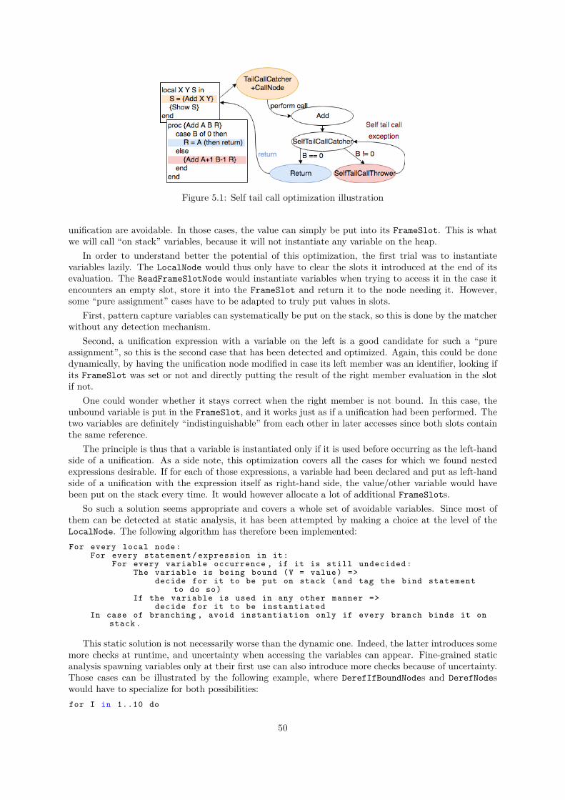
Figure 5.1: Self tail call optimization illustration
unification are avoidable. In those cases, the value can simply be put into its FrameSlot. This is whatwe will call “on stack” variables, because it will not instantiate any variable on the heap.
In order to understand better the potential of this optimization, the first trial was to instantiatevariables lazily. The LocalNode would thus only have to clear the slots it introduced at the end of itsevaluation. The ReadFrameSlotNode would instantiate variables when trying to access it in the case itencounters an empty slot, store it into the FrameSlot and return it to the node needing it. However,some “pure assignment” cases have to be adapted to truly put values in slots.
First, pattern capture variables can systematically be put on the stack, so this is done by the matcherwithout any detection mechanism.
Second, a unification expression with a variable on the left is a good candidate for such a “pureassignment”, so this is the second case that has been detected and optimized. Again, this could be donedynamically, by having the unification node modified in case its left member was an identifier, looking ifits FrameSlot was set or not and directly putting the result of the right member evaluation in the slotif not.
One could wonder whether it stays correct when the right member is not bound. In this case, theunbound variable is put in the FrameSlot, and it works just as if a unification had been performed. Thetwo variables are definitely “indistinguishable” from each other in later accesses since both slots containthe same reference.
The principle is thus that a variable is instantiated only if it is used before occurring as the left-handside of a unification. As a side note, this optimization covers all the cases for which we found nestedexpressions desirable. If for each of those expressions, a variable had been declared and put as left-handside of a unification with the expression itself as right-hand side, the value/other variable would havebeen put on the stack every time. It would however allocate a lot of additional FrameSlots.
So such a solution seems appropriate and covers a whole set of avoidable variables. Since most ofthem can be detected at static analysis, it has been attempted by making a choice at the level of theLocalNode. The following algorithm has therefore been implemented:For every local node:
For every statement / expression in it:For every variable occurrence , if it is still undecided :
The variable is being bound (V = value) =>decide for it to be put on stack (and tag the bind statement
to do so)If the variable is used in any other manner =>
decide for it to be instantiatedIn case of branching , avoid instantiation only if every branch binds it on
stack.
This static solution is not necessarily worse than the dynamic one. Indeed, the latter introduces somemore checks at runtime, and uncertainty when accessing the variables can appear. Fine-grained staticanalysis spawning variables only at their first use can also introduce more checks because of uncertainty.Those cases can be illustrated by the following example, where DerefIfBoundNodes and DerefNodeswould have to specialize for both possibilities:for I in 1..10 do
50
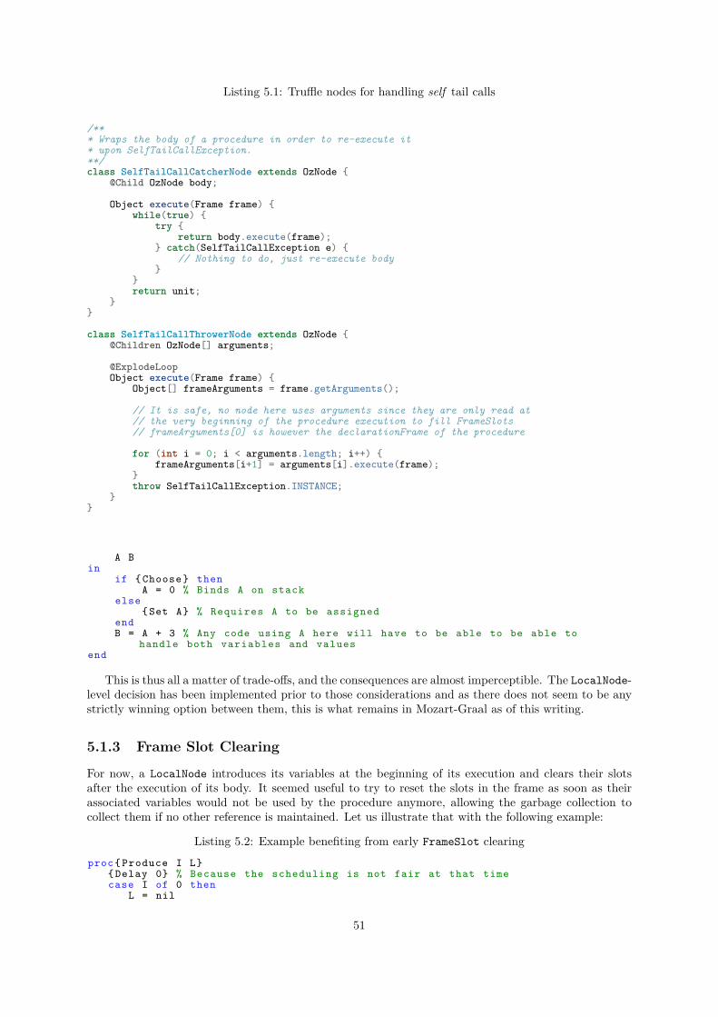
Listing 5.1: Truffle nodes for handling self tail calls
/*** Wraps the body of a procedure in order to re-execute it* upon SelfTailCallException.**/class SelfTailCallCatcherNode extends OzNode {
@Child OzNode body;
Object execute(Frame frame) {while(true) {
try {return body.execute(frame);
} catch(SelfTailCallException e) {// Nothing to do, just re-execute body
}}return unit;
}}
class SelfTailCallThrowerNode extends OzNode {@Children OzNode[] arguments;
@ExplodeLoopObject execute(Frame frame) {
Object[] frameArguments = frame.getArguments();
// It is safe, no node here uses arguments since they are only read at// the very beginning of the procedure execution to fill FrameSlots// frameArguments[0] is however the declarationFrame of the procedure
for (int i = 0; i < arguments.length; i++) {frameArguments[i+1] = arguments[i].execute(frame);
}throw SelfTailCallException.INSTANCE;
}}
A Bin
if { Choose } thenA = 0 % Binds A on stack
else{Set A} % Requires A to be assigned
endB = A + 3 % Any code using A here will have to be able to be able to
handle both variables and valuesend
This is thus all a matter of trade-offs, and the consequences are almost imperceptible. The LocalNode-level decision has been implemented prior to those considerations and as there does not seem to be anystrictly winning option between them, this is what remains in Mozart-Graal as of this writing.
5.1.3 Frame Slot Clearing
For now, a LocalNode introduces its variables at the beginning of its execution and clears their slotsafter the execution of its body. It seemed useful to try to reset the slots in the frame as soon as theirassociated variables would not be used by the procedure anymore, allowing the garbage collection tocollect them if no other reference is maintained. Let us illustrate that with the following example:
Listing 5.2: Example benefiting from early FrameSlot clearing
proc{ Produce I L}{Delay 0} % Because the scheduling is not fair at that timecase I of 0 then
L = nil
51
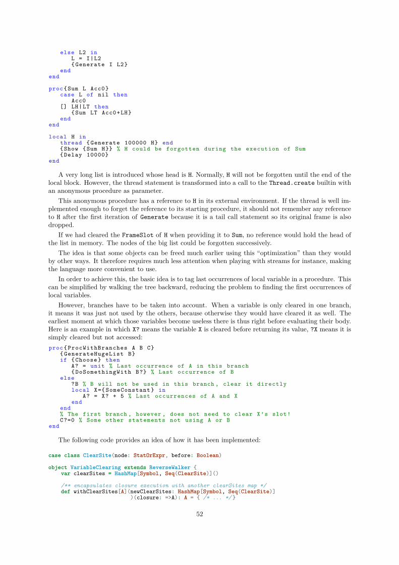
else L2 inL = I|L2{ Generate I L2}
endend
proc{Sum L Acc0}case L of nil then
Acc0[] LH|LT then
{Sum LT Acc0+LH}end
end
local H inthread { Generate 100000 H} end{Show {Sum H}} % H could be forgotten during the execution of Sum{Delay 10000}
end
A very long list is introduced whose head is H. Normally, H will not be forgotten until the end of thelocal block. However, the thread statement is transformed into a call to the Thread.create builtin withan anonymous procedure as parameter.
This anonymous procedure has a reference to H in its external environment. If the thread is well im-plemented enough to forget the reference to its starting procedure, it should not remember any referenceto H after the first iteration of Generate because it is a tail call statement so its original frame is alsodropped.
If we had cleared the FrameSlot of H when providing it to Sum, no reference would hold the head ofthe list in memory. The nodes of the big list could be forgotten successively.
The idea is that some objects can be freed much earlier using this “optimization” than they wouldby other ways. It therefore requires much less attention when playing with streams for instance, makingthe language more convenient to use.
In order to achieve this, the basic idea is to tag last occurrences of local variable in a procedure. Thiscan be simplified by walking the tree backward, reducing the problem to finding the first occurrences oflocal variables.
However, branches have to be taken into account. When a variable is only cleared in one branch,it means it was just not used by the others, because otherwise they would have cleared it as well. Theearliest moment at which those variables become useless there is thus right before evaluating their body.Here is an example in which X? means the variable X is cleared before returning its value, ?X means it issimply cleared but not accessed:proc{ ProcWithBranches A B C}
{ GenerateHugeList B}if { Choose } then
A? = unit % Last occurrence of A in this branch{ DoSomethingWith B?} % Last occurrence of B
else?B % B will not be used in this branch , clear it directlylocal X={ SomeConstant } in
A? = X? + 5 % Last occurrences of A and Xend
end% The first branch , however , does not need to clear X’s slot!C?=0 % Some other statements not using A or B
end
The following code provides an idea of how it has been implemented:
case class ClearSite(node: StatOrExpr, before: Boolean)
object VariableClearing extends ReverseWalker {var clearSites = HashMap[Symbol, Seq(ClearSite)]()
/** encapsulates closure execution with another clearSites map */def withClearSites[A](newClearSites: HashMap[Symbol, Seq(ClearSite)]
)(closure: =>A): A = { /* ... */ }
52
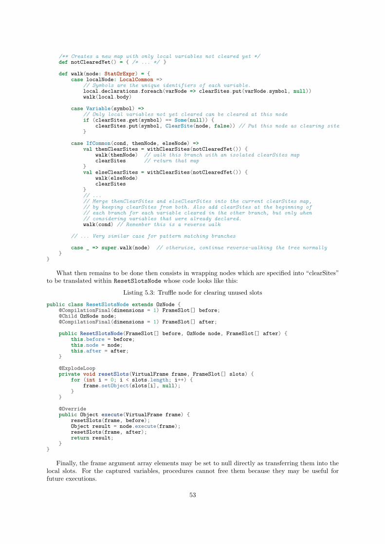
/** Creates a new map with only local variables not cleared yet */def notClearedYet() = { /* ... */ }
def walk(node: StatOrExpr) = {case localNode: LocalCommon =>
// Symbols are the unique identifiers of each variable.local.declarations.foreach(varNode => clearSites.put(varNode.symbol, null))walk(local.body)
case Variable(symbol) =>// Only local variables not yet cleared can be cleared at this nodeif (clearSites.get(symbol) == Some(null)) {
clearSites.put(symbol, ClearSite(node, false)) // Put this node as clearing site}
case IfCommon(cond, thenNode, elseNode) =>val thenClearSites = withClearSites(notClearedYet()) {
walk(thenNode) // walk this branch with an isolated clearSites mapclearSites // return that map
}val elseClearSites = withClearSites(notClearedYet()) {
walk(elseNode)clearSites
}// ...// Merge thenClearSites and elseClearSites into the current clearSites map,// by keeping clearSites from both. Also add clearSites at the beginning of// each branch for each variable cleared in the other branch, but only when// considering variables that were already declared.walk(cond) // Remember this is a reverse walk
// ... Very similar case for pattern matching branches
case _ => super.walk(node) // otherwise, continue reverse-walking the tree normally}
}
What then remains to be done then consists in wrapping nodes which are specified into “clearSites”to be translated within ResetSlotsNode whose code looks like this:
Listing 5.3: Truffle node for clearing unused slots
public class ResetSlotsNode extends OzNode {@CompilationFinal(dimensions = 1) FrameSlot[] before;@Child OzNode node;@CompilationFinal(dimensions = 1) FrameSlot[] after;
public ResetSlotsNode(FrameSlot[] before, OzNode node, FrameSlot[] after) {this.before = before;this.node = node;this.after = after;
}
@ExplodeLoopprivate void resetSlots(VirtualFrame frame, FrameSlot[] slots) {
for (int i = 0; i < slots.length; i++) {frame.setObject(slots[i], null);
}}
@Overridepublic Object execute(VirtualFrame frame) {
resetSlots(frame, before);Object result = node.execute(frame);resetSlots(frame, after);return result;
}}
Finally, the frame argument array elements may be set to null directly as transferring them into thelocal slots. For the captured variables, procedures cannot free them because they may be useful forfuture executions.
53
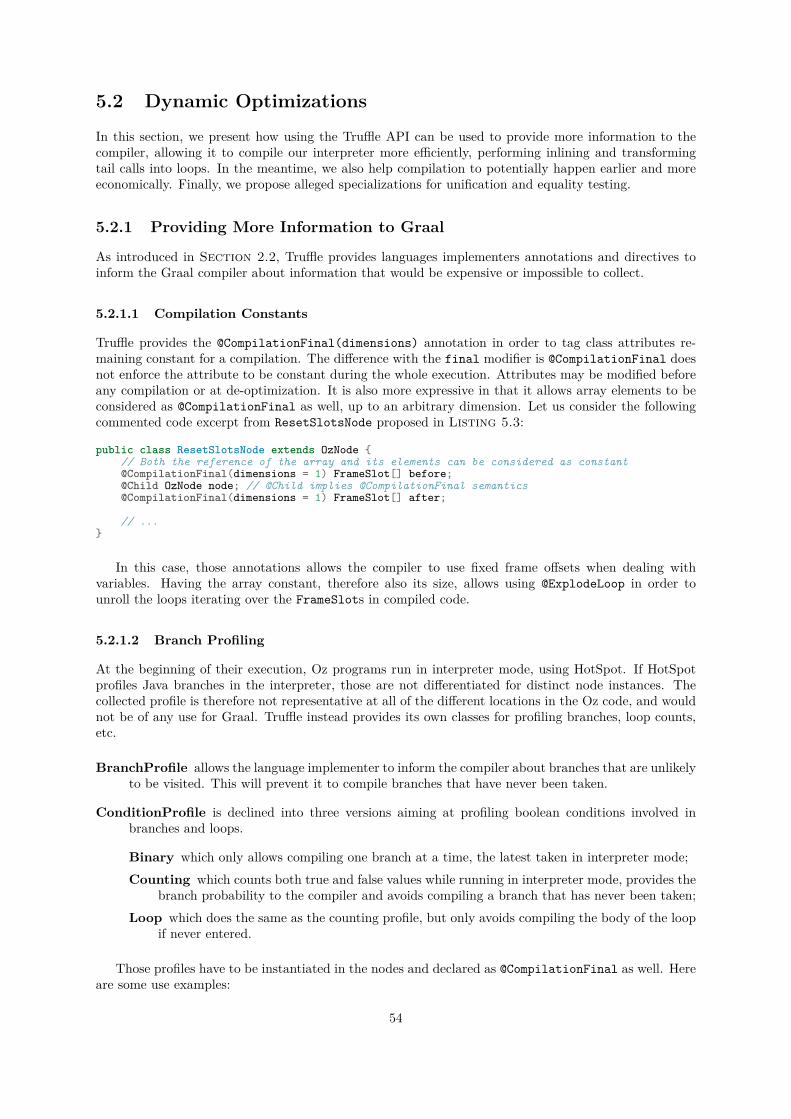
5.2 Dynamic Optimizations
In this section, we present how using the Truffle API can be used to provide more information to thecompiler, allowing it to compile our interpreter more efficiently, performing inlining and transformingtail calls into loops. In the meantime, we also help compilation to potentially happen earlier and moreeconomically. Finally, we propose alleged specializations for unification and equality testing.
5.2.1 Providing More Information to Graal
As introduced in Section 2.2, Truffle provides languages implementers annotations and directives toinform the Graal compiler about information that would be expensive or impossible to collect.
5.2.1.1 Compilation Constants
Truffle provides the @CompilationFinal(dimensions) annotation in order to tag class attributes re-maining constant for a compilation. The difference with the final modifier is @CompilationFinal doesnot enforce the attribute to be constant during the whole execution. Attributes may be modified beforeany compilation or at de-optimization. It is also more expressive in that it allows array elements to beconsidered as @CompilationFinal as well, up to an arbitrary dimension. Let us consider the followingcommented code excerpt from ResetSlotsNode proposed in Listing 5.3:
public class ResetSlotsNode extends OzNode {// Both the reference of the array and its elements can be considered as constant@CompilationFinal(dimensions = 1) FrameSlot[] before;@Child OzNode node; // @Child implies @CompilationFinal semantics@CompilationFinal(dimensions = 1) FrameSlot[] after;
// ...}
In this case, those annotations allows the compiler to use fixed frame offsets when dealing withvariables. Having the array constant, therefore also its size, allows using @ExplodeLoop in order tounroll the loops iterating over the FrameSlots in compiled code.
5.2.1.2 Branch Profiling
At the beginning of their execution, Oz programs run in interpreter mode, using HotSpot. If HotSpotprofiles Java branches in the interpreter, those are not differentiated for distinct node instances. Thecollected profile is therefore not representative at all of the different locations in the Oz code, and wouldnot be of any use for Graal. Truffle instead provides its own classes for profiling branches, loop counts,etc.
BranchProfile allows the language implementer to inform the compiler about branches that are unlikelyto be visited. This will prevent it to compile branches that have never been taken.
ConditionProfile is declined into three versions aiming at profiling boolean conditions involved inbranches and loops.
Binary which only allows compiling one branch at a time, the latest taken in interpreter mode;Counting which counts both true and false values while running in interpreter mode, provides the
branch probability to the compiler and avoids compiling a branch that has never been taken;Loop which does the same as the counting profile, but only avoids compiling the body of the loop
if never entered.
Those profiles have to be instantiated in the nodes and declared as @CompilationFinal as well. Hereare some use examples:
54
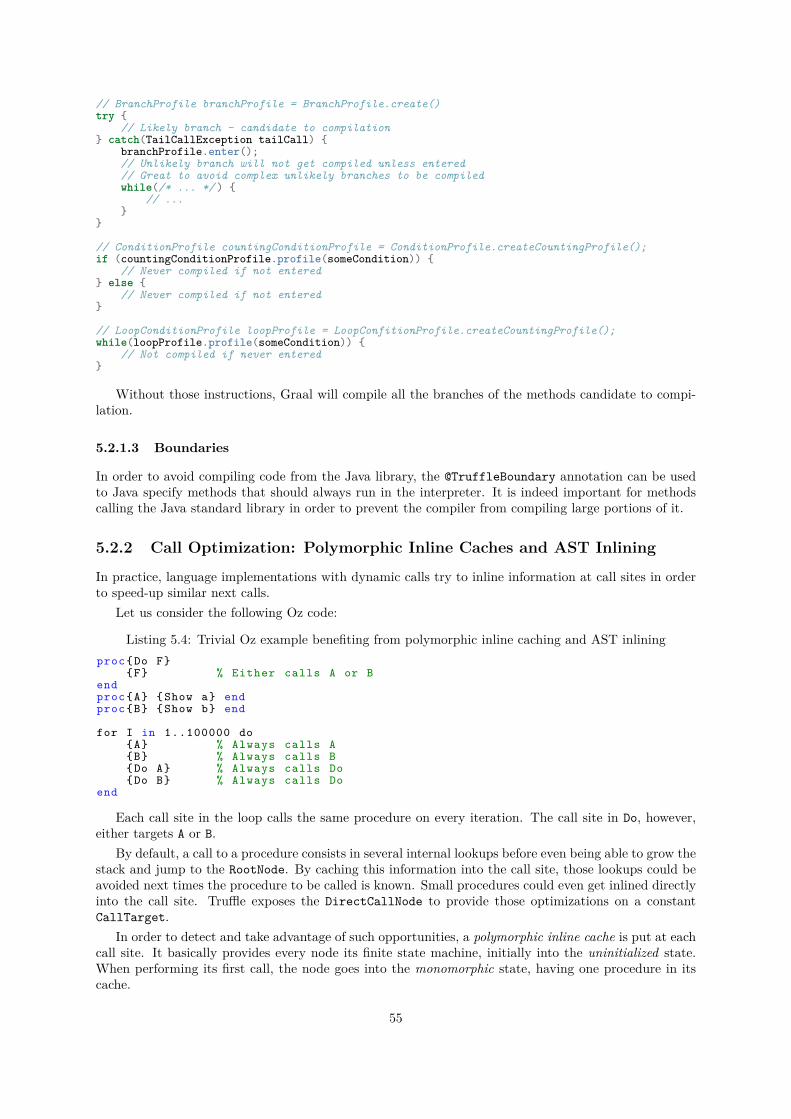
// BranchProfile branchProfile = BranchProfile.create()try {
// Likely branch - candidate to compilation} catch(TailCallException tailCall) {
branchProfile.enter();// Unlikely branch will not get compiled unless entered// Great to avoid complex unlikely branches to be compiledwhile(/* ... */ ) {
// ...}
}
// ConditionProfile countingConditionProfile = ConditionProfile.createCountingProfile();if (countingConditionProfile.profile(someCondition)) {
// Never compiled if not entered} else {
// Never compiled if not entered}
// LoopConditionProfile loopProfile = LoopConfitionProfile.createCountingProfile();while(loopProfile.profile(someCondition)) {
// Not compiled if never entered}
Without those instructions, Graal will compile all the branches of the methods candidate to compi-lation.
5.2.1.3 Boundaries
In order to avoid compiling code from the Java library, the @TruffleBoundary annotation can be usedto Java specify methods that should always run in the interpreter. It is indeed important for methodscalling the Java standard library in order to prevent the compiler from compiling large portions of it.
5.2.2 Call Optimization: Polymorphic Inline Caches and AST Inlining
In practice, language implementations with dynamic calls try to inline information at call sites in orderto speed-up similar next calls.
Let us consider the following Oz code:
Listing 5.4: Trivial Oz example benefiting from polymorphic inline caching and AST inliningproc{Do F}
{F} % Either calls A or Bendproc{A} {Show a} endproc{B} {Show b} end
for I in 1..100000 do{A} % Always calls A{B} % Always calls B{Do A} % Always calls Do{Do B} % Always calls Do
end
Each call site in the loop calls the same procedure on every iteration. The call site in Do, however,either targets A or B.
By default, a call to a procedure consists in several internal lookups before even being able to grow thestack and jump to the RootNode. By caching this information into the call site, those lookups could beavoided next times the procedure to be called is known. Small procedures could even get inlined directlyinto the call site. Truffle exposes the DirectCallNode to provide those optimizations on a constantCallTarget.
In order to detect and take advantage of such opportunities, a polymorphic inline cache is put at eachcall site. It basically provides every node its finite state machine, initially into the uninitialized state.When performing its first call, the node goes into the monomorphic state, having one procedure in itscache.
55
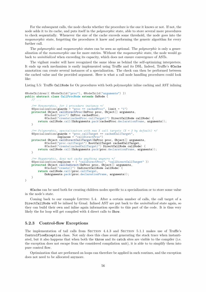
For the subsequent calls, the node checks whether the procedure is the one it knows or not. If not, thenode adds it to its cache, and puts itself in the polymorphic state, able to store several more proceduresto check sequentially. Whenever the size of the cache exceeds some threshold, the node goes into themegamorphic state, forgetting the procedures it knew and performing the generic algorithm for everyfurther call.
The polymorphic and megamorphic states can be seen as optional. The polymorphic is only a gener-alization of the monomorphic one for more entries. Without the megamorphic state, the node would goback to uninitialized when exceeding its capacity, which does not ensure convergence of ASTs.
The vigilant reader will have recognized the same ideas as behind the self-optimizing interpreters.It ends up such mechanism is easily implemented using Truffle and its DSL. Indeed, Truffle’s @Cacheannotation can create several instances of a specialization. The check can then be performed betweenthe cached value and the provided argument. Here is what a call node handling procedures could looklike:
Listing 5.5: Truffle CallNode for Oz procedures with both polymorphic inline caching and AST inlining
@NodeChildren({ @NodeChild("proc"), @NodeChild("arguments") })public abstract class CallProcNode extends OzNode {
// ...
/** Monomorphic, for 1 procedure instance */@Specialization(guards = "proc == cachedProc", limit = "1")protected Object callDirectProc(OzProc proc, Object[] arguments,
@Cached("proc") OzProc cachedProc,@Cached("create(cachedProc.callTarget)") DirectCallNode callNode) {
return callNode.call(OzArguments.pack(cachedProc.declarationFrame, arguments));}
/** Polymorphic, specialization with max X call targets (X = 3 by default) */@Specialization(guards = "proc.callTarget == cachedCallTarget",
replaces = "callDirectProc")protected Object callDirectCallTarget(OzProc proc, Object[] arguments,
@Cached("proc.callTarget") RootCallTarget cachedCallTarget,@Cached("create(cachedCallTarget)") DirectCallNode callNode) {
return callNode.call(OzArguments.pack(proc.declarationFrame, arguments));}
/** Megamorphic, does not cache anything anymore */@Specialization(replaces = { "callDirectProc", "callDirectCallTarget" })protected Object callIndirect(OzProc proc, Object[] arguments,
@Cached("create()") IndirectCallNode callNode) {return callNode.call(proc.callTarget,
OzArguments.pack(proc.declarationFrame, arguments));}
}
@Cache can be used both for creating children nodes specific to a specialization or to store some valuein the node’s state.
Coming back to our example Listing 5.4. After a certain number of calls, the call target of aDirectCallNode will be inlined by Graal. Inlined AST are put back to the uninitialized state again, sothey can build their own and inline again information specific to this part of the code. It is thus verylikely the for loop will get compiled with 4 direct calls to Show.
5.2.3 Control-flow Exceptions
The implementation of tail calls from Section 4.4.3 and Section 5.1.1 makes use of Truffle’sControlFlowException class. Not only does this class avoid generating the stack trace when instanti-ated, but it also happens that when both the throw and its catch sites are visible to the compiler (i.e.the exception does not escape from the considered compilation unit), it is able to to simplify them intopure control flow.
Optimization that are performed on loops can therefore be applied in such routines, and the exceptiondoes not need to be allocated anymore.
56
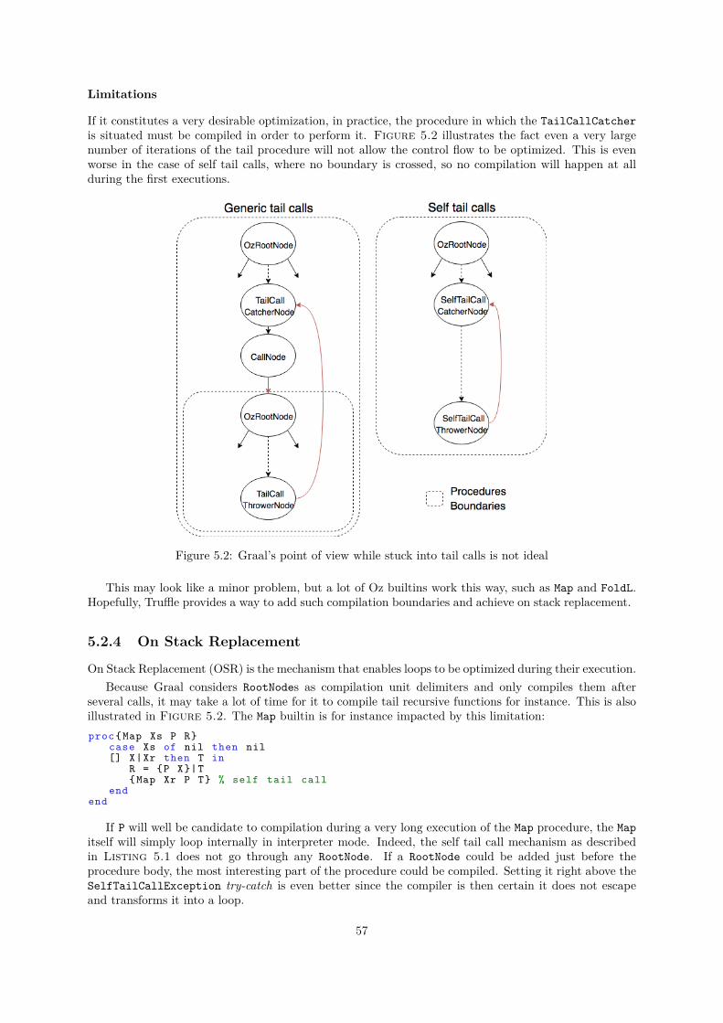
Limitations
If it constitutes a very desirable optimization, in practice, the procedure in which the TailCallCatcheris situated must be compiled in order to perform it. Figure 5.2 illustrates the fact even a very largenumber of iterations of the tail procedure will not allow the control flow to be optimized. This is evenworse in the case of self tail calls, where no boundary is crossed, so no compilation will happen at allduring the first executions.
Figure 5.2: Graal’s point of view while stuck into tail calls is not ideal
This may look like a minor problem, but a lot of Oz builtins work this way, such as Map and FoldL.Hopefully, Truffle provides a way to add such compilation boundaries and achieve on stack replacement.
5.2.4 On Stack Replacement
On Stack Replacement (OSR) is the mechanism that enables loops to be optimized during their execution.Because Graal considers RootNodes as compilation unit delimiters and only compiles them after
several calls, it may take a lot of time for it to compile tail recursive functions for instance. This is alsoillustrated in Figure 5.2. The Map builtin is for instance impacted by this limitation:proc{Map Xs P R}
case Xs of nil then nil[] X|Xr then T in
R = {P X}|T{Map Xr P T} % self tail call
endend
If P will well be candidate to compilation during a very long execution of the Map procedure, the Mapitself will simply loop internally in interpreter mode. Indeed, the self tail call mechanism as describedin Listing 5.1 does not go through any RootNode. If a RootNode could be added just before theprocedure body, the most interesting part of the procedure could be compiled. Setting it right above theSelfTailCallException try-catch is even better since the compiler is then certain it does not escapeand transforms it into a loop.
57
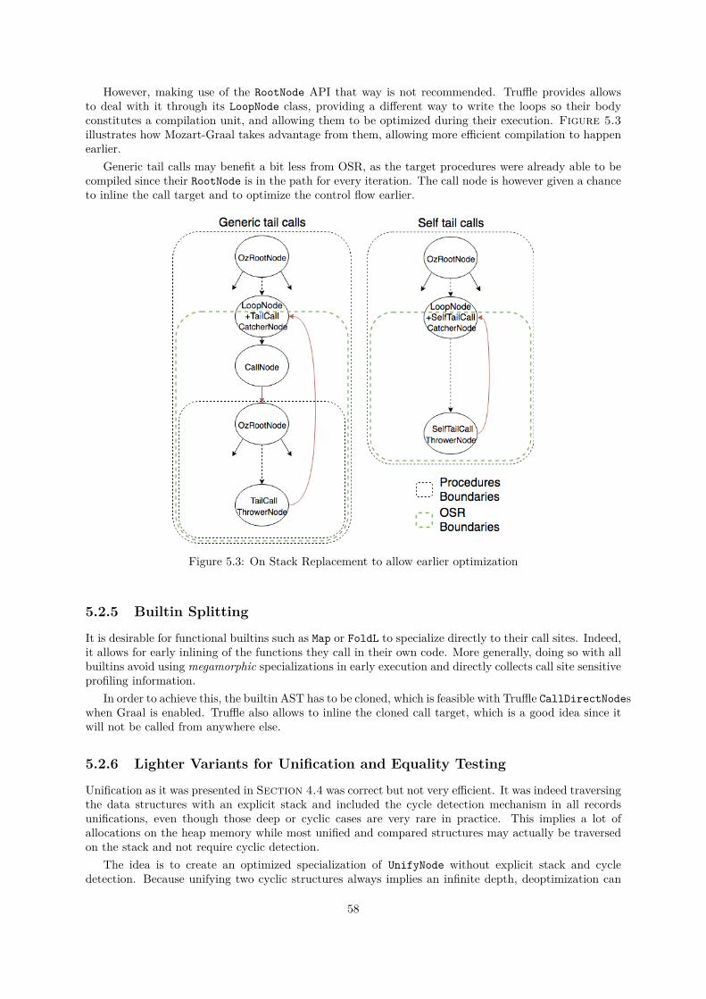
However, making use of the RootNode API that way is not recommended. Truffle provides allowsto deal with it through its LoopNode class, providing a different way to write the loops so their bodyconstitutes a compilation unit, and allowing them to be optimized during their execution. Figure 5.3illustrates how Mozart-Graal takes advantage from them, allowing more efficient compilation to happenearlier.
Generic tail calls may benefit a bit less from OSR, as the target procedures were already able to becompiled since their RootNode is in the path for every iteration. The call node is however given a chanceto inline the call target and to optimize the control flow earlier.
Figure 5.3: On Stack Replacement to allow earlier optimization
5.2.5 Builtin Splitting
It is desirable for functional builtins such as Map or FoldL to specialize directly to their call sites. Indeed,it allows for early inlining of the functions they call in their own code. More generally, doing so with allbuiltins avoid using megamorphic specializations in early execution and directly collects call site sensitiveprofiling information.
In order to achieve this, the builtin AST has to be cloned, which is feasible with Truffle CallDirectNodeswhen Graal is enabled. Truffle also allows to inline the cloned call target, which is a good idea since itwill not be called from anywhere else.
5.2.6 Lighter Variants for Unification and Equality Testing
Unification as it was presented in Section 4.4 was correct but not very efficient. It was indeed traversingthe data structures with an explicit stack and included the cycle detection mechanism in all recordsunifications, even though those deep or cyclic cases are very rare in practice. This implies a lot ofallocations on the heap memory while most unified and compared structures may actually be traversedon the stack and not require cyclic detection.
The idea is to create an optimized specialization of UnifyNode without explicit stack and cycledetection. Because unifying two cyclic structures always implies an infinite depth, deoptimization can
58
simply happen when this depth exceeds some threshold, the same we think would suffice to avoid thestack overflow in simple deep cases. On one hand, this threshold must not be too low because nodes thatdo not require it would make use of cycle detection and this is what we try to avoid. On the other hand,having it too big risks to let stack overflow happen and could waste a lot of time before deoptimization.
Let us consider a cyclic record with N features whose last one is a reference to itself:R = record (1 2 3 ... N-1 R)Q = record (1 2 3 ... N-1 Q)R = Q
By going depth-first, the complexity of reaching depth d is O(dN). But imagine first features couldthemselves be complex structures as in the following:SubR = record (1 2 3 ... N)R = record (SubR SubR ... SubR R)
SubQ = record (1 2 3 ... N)Q = record (SubQ SubQ ... SubQ Q)
R = Q
This would take much more operations (O(dN2)), while cycle detection would have allow to only walkonce through SubR and SubQ and would have remembered them to be equivalent. Arbitrarily pathologicalcases can be forged.
In order to avoid this potentially huge overhead before deoptimization, this is the number of sub-unifications rather than the depth that is bounded. So a threshold n is always reached in Θ(n) sub-unifications.
The implementation relies on a base node class DFSUnifyNode with different specializations for han-dling the simple cases in a compiler-friendly manner. It specializes for two unbound variables to link,one unbound variable to bind or two bound variables with values. Some can be compared in a shallowmanner, but records are unified recursively, which leads to stack overflows when they are deep circular.
This class is then extended by two other node classes, DepthLimitedUnifyNode and OnHeapUnifyNode,both only creating some state when unifying two records. The state of the first consists of a number ofsub-unifications after which it deoptimizes, while the state of the second consists of the explicit stack forthe traversal and the set of already encountered pairs of variables.
A final node class, GenericUnifyNode, acts as dispatcher between both, falling back on theOnHeapUnifyNode only once the DepthLimitedUnifyNode has thrown an exception stating its thresholdhas been reached. It may happen that unbound variables get affected by the limited depth unificationbefore deoptimization and end up being seen as bound to the cycle detecting unification. This does notcreate inconsistencies because unification is idempotent.
A very similar mechanism is used for equality testing through the DFSEqualNode,DepthLimitedEqualNode, OnHeapEqualNode and GenericEqualNode. Pattern matching can stillsimply use the DFSEqualNode for its constants, since at least the pattern is not circular. AGenericEqualNode is however required for the escaped variable patterns as they might be circular.
59

60
Chapter 6
Evaluation
In this chapter, we first evaluate the improvements brought to Mozart-Graal. We start with the additionalinformation provided from the static analysis allowing to remove part of the dataflow variables and toavoid memory leaks. We then consider the different optimizations around tail calls. As unification andequality tests were efficient but not general enough, the performance degradation for achieving generalitywill be measured. A section will then be dedicated to the evaluation of inlining and the different featuresarticulated around it.
Finally, we evaluate more globally the current state of Mozart-Graal and compare it with Mozart 1and 2 on different aspects. We will see that if it can already be competitive in some cases, there is stillroom for improvement.
6.1 Methodology
Two kinds of programs will help us to obtain results for our implementation: micro-benchmarks made ofspecific features and a realistic project. Those Oz programs and a tool for running them and collectingtheir output has been developed and is hosted on GitHub at [18]. It also comprises the Jupyter notebookwe have used [19] for data visualization. The project we have considered is the Project 2014 [32] providedby Guillaume Maudoux. All the codes have been instrumented to print clock times and to be configurableby the runner program. As discussed in Appendix A.1, the impact of measuring time as been verifiedto be negligible with respect to the interpretation we make of those collected times.
The configuration is done through the bench_*.txt files of which each line describes a program torun with given parameters. Different categories of parameters are covered:
1. The Oz implementation to run the program with. The benchmarks used in this dissertation arewritten to run on Mozart 1, Mozart 2 and Mozart-Graal.
2. Options of the JVM or of the Graal compiler when running the program under Mozart-Graal.3. Options that are defined in Mozart-Graal, for disabling optimizations for instance.4. Actual variables in the main functor. This may help to tune number of iterations, complexity of
structures, ...
All of those programs have been run on a dedicated server through Secure Shell (SSH) connection.Only one has been run at a time, with the minimal amount of concurrent services running. This serverruns under Ubuntu Server 14.04 LTS and is equipped of an Intel(R) Core(TM) i5-2400 CPU (quad core)at 3.10GHz and 4x4096MB RAM at 1333MHz.
Mozart 1 is used as of its 1.4.0-2008-07-03-GENERIC-i386 release available at https://sourceforge.net/projects/mozart-oz/files/v1/.
Mozart 2 is used as of its 2.0.0-alpha.0 build 4105 release available at https://sourceforge.net/projects/mozart-oz/files/v2.0.0-alpha.0/.
61

Mozart-Graal is used as of this branch: https://github.com/mistasse/mozart-graal/tree/memoire-final. Truffle has been used as of this commit: https://github.com/eregon/truffle/tree/c3ae06dbe4c6008f83c3fab69e22e7095a30f929 and Graal as of this commit: https://github.com/eregon/graal-core/tree/1236bbd1691733995623f3f42f9ac3984300e437.
Because we are mostly interested in peak performance, all our programs are running the main codesection several times, the exact number depending on the difficulty of the task. Under some circumstancescode may get compiled during the first iteration or may not get compiled during the whole execution.This will be discussed in due course.
Uncompiled code and compilation itself also require more memory allocation which implies garbagecollection. If this affects a lot early iterations, this usually becomes stable or periodic at some point.The default parameters of the benchmarks are set accordingly in order to ensure each program reachesits stationary performance during at least half the iterations. Modifying some of the parameters mayhowever influence this behavior.
Comparison between optimizations will mostly be performed based on peak performance, which wedecided to measure as the mean iteration time, considering only the second half of all the iterations. Itend up being insensitive to the early noise but still gets affected by periodic garbage collection. Moremetrics will also be used here and there such as instantiated variables, early iterations profiles, or totalexecution times of the programs. Most of the time, iteration times are averaged over several runs. Thisis achieved by taking the mean of analogous iterations of the different runs.
In some cases, Graal IR graphs are used to discuss whether the compiled code reaches the quality weexpect or not. Those are collected and printed using the Ideal Graph Visualizer [43], and can be foundin Appendix A.4. If no part of this dissertation will be dedicated to the reading of those graphs, theyare annotated in order to provide some insights about what is happening. Part of [24] is dedicated toexplaining the nodes more deeply. The very new [44] also provides insights about analyzing such graphsapplied to the case of TruffleRuby.
The Benchmark Programs
As stated here before, several programs will be used in order to assess the performance of our imple-mentation. Each consists of some main task of adjustable complexity and a loop executing it for a givennumber of iterations. This loop also reports the time taken for each iteration, i.e. execution of the task.
Add The Add program consists in adding two numbers by incrementing one of them and decrementingthe other in a tail recursive manner. Its complexity parameter is the number to decrement N, whilethe other always starts at 0 for convenience.
Map The Map program consists in applying a small arithmetic function on every element of a list. Bydefault, the arithmetic function is a simple multiplication with the constant 11. The complexityparameter is the length N of the input list.
Flatten The Flatten program consists in flattening a list of arbitrary size and depth. The complexityparameter is the number N of sublists of depth 5 in that list.
PingPong The PingPong program consists in two threads interacting through a stream, each placingan atom in it one after the other until a certain number of atoms have been placed. The parameteris the number of atoms N each thread puts in the stream.
Sieve The Sieve program consists in computing the list of prime numbers under an arbitrary threshold Nin a concurrent manner, each discovered prime number having its own thread filtering the numbersit can divide and passing others to next threads. The parameters also comprise whether to stopcreating threads at
√N or not, and whether the functions have to be lazy or not.
Project2014 The Project2014 program consists in executing Project 2014 without writing the final fileto the disk. The partition joie.dj.oz will be considered by default. It makes heavy use of lists,Map, Flatten and user-defined functions.
62
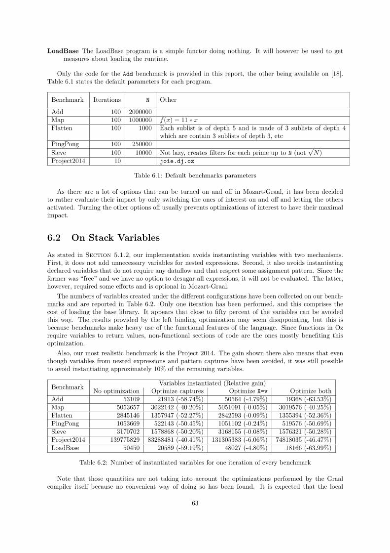
LoadBase The LoadBase program is a simple functor doing nothing. It will however be used to getmeasures about loading the runtime.
Only the code for the Add benchmark is provided in this report, the other being available on [18].Table 6.1 states the default parameters for each program.
Benchmark Iterations N Other
Add 100 2000000Map 100 1000000 f(x) = 11 ∗ xFlatten 100 1000 Each sublist is of depth 5 and is made of 3 sublists of depth 4
which are contain 3 sublists of depth 3, etcPingPong 100 250000Sieve 100 10000 Not lazy, creates filters for each prime up to N (not
√N)
Project2014 10 joie.dj.oz
Table 6.1: Default benchmarks parameters
As there are a lot of options that can be turned on and off in Mozart-Graal, it has been decidedto rather evaluate their impact by only switching the ones of interest on and off and letting the othersactivated. Turning the other options off usually prevents optimizations of interest to have their maximalimpact.
6.2 On Stack Variables
As stated in Section 5.1.2, our implementation avoids instantiating variables with two mechanisms.First, it does not add unnecessary variables for nested expressions. Second, it also avoids instantiatingdeclared variables that do not require any dataflow and that respect some assignment pattern. Since theformer was “free” and we have no option to desugar all expressions, it will not be evaluated. The latter,however, required some efforts and is optional in Mozart-Graal.
The numbers of variables created under the different configurations have been collected on our bench-marks and are reported in Table 6.2. Only one iteration has been performed, and this comprises thecost of loading the base library. It appears that close to fifty percent of the variables can be avoidedthis way. The results provided by the left binding optimization may seem disappointing, but this isbecause benchmarks make heavy use of the functional features of the language. Since functions in Ozrequire variables to return values, non-functional sections of code are the ones mostly benefiting thisoptimization.
Also, our most realistic benchmark is the Project 2014. The gain shown there also means that eventhough variables from nested expressions and pattern captures have been avoided, it was still possibleto avoid instantiating approximately 10% of the remaining variables.
Benchmark Variables instantiated (Relative gain)No optimization Optimize captures Optimize X=v Optimize both
Add 53109 21913 (-58.74%) 50564 (-4.79%) 19368 (-63.53%)Map 5053657 3022142 (-40.20%) 5051091 (-0.05%) 3019576 (-40.25%)Flatten 2845146 1357947 (-52.27%) 2842593 (-0.09%) 1355394 (-52.36%)PingPong 1053669 522143 (-50.45%) 1051102 (-0.24%) 519576 (-50.69%)Sieve 3170702 1578868 (-50.20%) 3168155 (-0.08%) 1576321 (-50.28%)Project2014 139775829 83288481 (-40.41%) 131305383 (-6.06%) 74818035 (-46.47%)LoadBase 50450 20589 (-59.19%) 48027 (-4.80%) 18166 (-63.99%)
Table 6.2: Number of instantiated variables for one iteration of every benchmark
Note that those quantities are not taking into account the optimizations performed by the Graalcompiler itself because no convenient way of doing so has been found. It is expected that the local
63
variables not escaping from compiled procedures would be removed. As to whether variables are actuallyescaping or not, it all depends on the scope of the compiler which depends on how inlining is performed.
Conclusion
On stack variables constitute a first step towards a more parsimonious use of dataflow variables. Mostof them would be avoided when critical sections get JIT compiled, but the quality of this optimizationdepends on the compiler’s point of view. Making sure we do not rely on the JIT compiler to avoid themajority of non-dataflow variables therefore seems to be a good start.
6.3 Variable Selection
Prior to this master’s thesis, the external environment of each procedure was not a “filtered” copy, butrather a pointer to the upper declaring local environment. Just like the alternative solution presentedin Section 4.2.2. This means that releasing variables as in Section 5.1.3 was impossible, thereforeleading to memory leaks.
An example is that heads of streams were more difficult to drop. Let us take this example:declareproc {Ping S}
case S of pong|A thenA = ping|_{Ping A.2}
endendproc {Pong S}
case S of ping|A thenA = ping|_
{Ping A.2}end
end
local S = pong|_ inthread {Ping S} endthread {Pong S.2} end
end
Because the variables of the local are stored in the frame of the main procedure, the Ping and Pongwere in fact maintaining references to the head directly. It is possible to write programs achieving itwithout leaks by encapsulating the stream creation in a procedure, but this is uncomfortable as thisrequires special attention from the developer.
Now, references are dropped correctly thanks to variable selection which provides the dependenciesfor procedures in a more refined manner. The local block can thus clear its slot while the other threadsare able to forget the anonymous procedure they have been started with. No reference to S is maintainedanymore, the garbage collector can therefore discard the beginning of the stream from memory.
6.3.1 Frame Slot Clearing
We have found that this was however still too limiting. Indeed, developers still have to pay attentionto ensure leaving the local block before the stream gets too big. This means the following code is alsoleaking, even though it is clear the intention was to release the head of the stream:declareproc {Ping S}
case S of pong|A thenA = ping|_{Ping A.2}
endendproc {Pong S I}
case S of ping|A andthen I >= 0 thenA = ping|_{Pong A.2}
64
endendT0 T1
local S = _|_ inthread {Ping S} endT0 = {Time}{Pong S.2 2000000} % maintains a reference to S, but could clear it when
computing S.2endT1 = {Time}{Show T1 -T0}
This is even more disturbing as if the Pong call had been the last statement, the memory leak wouldnot have happened. This is why frame slot clearing has been introduced in order to release references tolocal variables as early as possible, right after having evaluated their last identifier.
As a side note, clearing the frame slots should not influence the generated code since the compiler isalready aware variable occurrences. It is however necessary for the interpreter mode that does not havea complete vision on them.
The impact can be evaluated on our PingPong program by running 1 iteration with N = 106 with theJVM option -Xmx100m for restricting the heap size to 100MB. The version clearing the slots terminateswhile the other tries to store the whole stream and ends up crashing.
Limitations
Frame slot clearing takes care of freeing all slots, even though it is sometimes obvious the procedure isgoing to end and no statement is susceptible to block it for a long time. Improvements could reduce thenumber of clearing nodes by removing those that are negligible in that sense and by merging those thatare separated only by non-blocking statements.
Some AST nodes also directly keep references to values into their state because the Graal compilercould not see through weak references when they have been written. It could thus not optimize thosenodes as well when using them. As it is not the case anymore, some node classes should be adapted inorder for Mozart-Graal to be totally memory-friendly. Classical calls have however already been updated.
Conclusion
Variable selection thus makes Mozart-Graal much more friendly with the garbage collection than thehierarchy of frames by allowing it to dissociate variables in the same frame. This also allows clearingframe slots to free references as soon as they are not used, which relieves the developer from havingto think about escaping local blocks declaring a stream before doing computation on it. Those twooptimizations make the whole implementation much more predictable when programming.
6.3.2 Tail Calls, Loops and On Stack Replacement
Prior to our work, tail calls were not implemented. This is therefore one of the first contributions realizedfor this master’s thesis. We do not consider benchmarking in absence of tail call optimization becauseserious tasks making use of them simply crash when doing so. We rather evaluate the different variantsof this optimization and their treatment by the compiler.
We will first illustrate the performance improvement brought by self tail calls and OSR using the Addmicro-benchmark from Listing A.1. We will then evaluate their impact on the Project 2014 from [32].
The peak iteration times are reported in Table 6.3, and Figure 6.1 plots iteration times obtainedwith those different sets of optimizations. The experiments on the left do not perform self tail calldetection, which means only the generic tail call optimization is applied, while experiments in the rightpart considers them. Each of those configuration is considered with and without OSR.
Let us discuss the four curves independently.
Case #1 no self tail calls and no OSR : the Add function gets compiled, but the exception mecha-
65
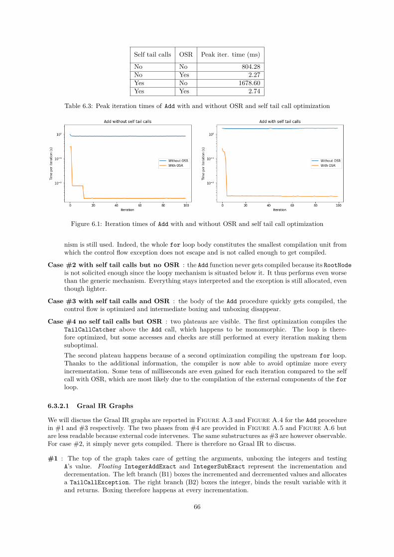
Self tail calls OSR Peak iter. time (ms)
No No 804.28No Yes 2.27Yes No 1678.60Yes Yes 2.74
Table 6.3: Peak iteration times of Add with and without OSR and self tail call optimization
Figure 6.1: Iteration times of Add with and without OSR and self tail call optimization
nism is still used. Indeed, the whole for loop body constitutes the smallest compilation unit fromwhich the control flow exception does not escape and is not called enough to get compiled.
Case #2 with self tail calls but no OSR : the Add function never gets compiled because its RootNodeis not solicited enough since the loopy mechanism is situated below it. It thus performs even worsethan the generic mechanism. Everything stays interpreted and the exception is still allocated, eventhough lighter.
Case #3 with self tail calls and OSR : the body of the Add procedure quickly gets compiled, thecontrol flow is optimized and intermediate boxing and unboxing disappear.
Case #4 no self tail calls but OSR : two plateaus are visible. The first optimization compiles theTailCallCatcher above the Add call, which happens to be monomorphic. The loop is there-fore optimized, but some accesses and checks are still performed at every iteration making themsuboptimal.The second plateau happens because of a second optimization compiling the upstream for loop.Thanks to the additional information, the compiler is now able to avoid optimize more everyincrementation. Some tens of milliseconds are even gained for each iteration compared to the selfcall with OSR, which are most likely due to the compilation of the external components of the forloop.
6.3.2.1 Graal IR Graphs
We will discuss the Graal IR graphs are reported in Figure A.3 and Figure A.4 for the Add procedurein #1 and #3 respectively. The two phases from #4 are provided in Figure A.5 and Figure A.6 butare less readable because external code intervenes. The same substructures as #3 are however observable.For case #2, it simply never gets compiled. There is therefore no Graal IR to discuss.
#1 : The top of the graph takes care of getting the arguments, unboxing the integers and testingA’s value. Floating IntegerAddExact and IntegerSubExact represent the incrementation anddecrementation. The left branch (B1) boxes the incremented and decremented values and allocatesa TailCallException. The right branch (B2) boxes the integer, binds the result variable with itand returns. Boxing therefore happens at every incrementation.
66
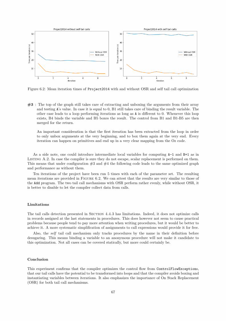
Figure 6.2: Mean iteration times of Project2014 with and without OSR and self tail call optimization
#3 : The top of the graph still takes care of extracting and unboxing the arguments from their arrayand testing A’s value. In case it is equal to 0, B1 still takes care of binding the result variable. Theother case leads to a loop performing iterations as long as A is different to 0. Whenever this loopexists, B4 binds the variable and B5 boxes the result. The control from B1 and B1-B5 are thenmerged for the return.
An important consideration is that the first iteration has been extracted from the loop in orderto only unbox arguments at the very beginning, and to box them again at the very end. Everyiteration can happen on primitives and end up in a very clear mapping from the Oz code.
As a side note, one could introduce intermediate local variables for computing A-1 and B+1 as inListing A.2. In case the compiler is sure they do not escape, scalar replacement is performed on them.This means that under configuration #3 and #4 the following code leads to the same optimized graphand performance as without them.
Ten iterations of the project have been run 5 times with each of the parameter set. The resultingmean iterations are provided in Figure 6.2. We can attest that the results are very similar to those ofthe Add program. The two tail call mechanisms with OSR perform rather evenly, while without OSR, itis better to disable to let the compiler collect data from calls.
Limitations
The tail calls detection presented in Section 4.4.3 has limitations. Indeed, it does not optimize callsin records assigned at the last statements in procedures. This does however not seem to cause practicalproblems because people tend to pay more attention when writing procedures, but it would be better toachieve it. A more systematic simplification of assignments to call expressions would provide it for free.
Also, the self tail call mechanism only tracks procedures by the name in their definition beforedesugaring. This means binding a variable to an anonymous procedure will not make it candidate tothis optimization. Not all cases can be covered statically, but more could certainly be.
Conclusion
This experiment confirms that the compiler optimizes the control flow from ControlFlowExceptions,that our tail calls have the potential to be transformed into loops and that the compiler avoids boxing andinstantiating variables between iterations. It also emphasizes the importance of On Stack Replacement(OSR) for both tail call mechanisms.
67
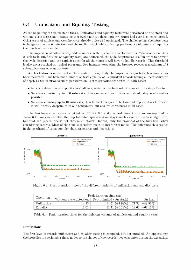
6.4 Unification and Equality Testing
At the beginning of this master’s thesis, unifications and equality tests were performed on the stack andwithout cycle detection, because neither cyclic nor too deep data-structures had ever been encountered.Other cases of unifications were however already quite well optimized. The challenge has therefore beento integrate the cycle detection and the explicit stack while affecting performance of cases not requiringthem as least as possible.
The implemented solution only adds counters on the specializations for records. Whenever more than20 sub-tasks (unifications or equality tests) are performed, the node deoptimizes itself in order to providethe cycle detection and the explicit stack for all the times it will have to handle records. This thresholdis also never reached on typical programs. For instance, executing the browser reaches a maximum of 8sub-unifications or equality tests.
As this feature is never used in the standard library, only the impact on a synthetic benchmark hasbeen measured. This benchmark unifies or tests equality of 2 equivalent records having a linear structureof depth 15 ten thousands times per iteration. Three scenarios are tested in both cases:
• No cycle detection or explicit stack fallback, which is the base solution we want to stay close to.• Sub-task counting up to 100 sub-tasks. This one never deoptimizes and should stay as efficient aspossible.
• Sub-task counting up to 10 sub-tasks, then fallback on cycle detection and explicit stack traversal.It will directly deoptimize in our benchmark but ensures correctness in all cases.
The benchmark results are provided in Figure 6.3 and the peak iteration times are reported inTable 6.4. We can see that the depth-limited specialization stays much closer to the base algorithm,but that the general one is not that much slower. Indeed, only the traversal of the first level whenconsidering records. Most of the time is therefore spent in interpreter mode. The difference thus residesin the overhead of using complex data-structures and algorithms.
Figure 6.3: Mean iteration times of the different variants of unification and equality tests
Operation Peak iteration time (ms)Without cycle detection Depth limited (On stack) On heap
Unification 14.23 14.51 (+1.98%) 21.33 (+49.86%)Equality 11.01 11.71 (+6.29%) 18.62 (+69.11%)
Table 6.4: Peak iteration times for the different variants of unification and equality tests
Limitations
The first level of records unification and equality testing is compiled, but not unrolled. An opportunitytherefore lies in specializing those nodes to the shapes of the records they encounter during the execution.
68
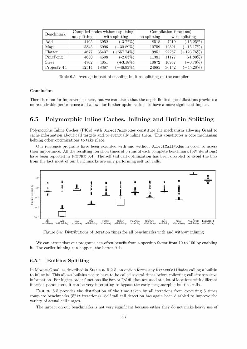
Benchmark Compiled nodes without splitting Compilation time (ms)no splitting with splitting no splitting with splitting
Add 4105 3952 (-3.72%) 8518 7219 (-15.25%)Map 5345 6996 (+30.89%) 10759 12391 (+15.17%)Flatten 4677 35437 (+657.74%) 9951 22267 (+123.76%)PingPong 4630 4508 (-2.63%) 11381 11177 (-1.80%)Sieve 4702 4851 (+3.18%) 10872 10957 (+0.78%)Project2014 12514 18387 (+46.93%) 24885 36152 (+45.28%)
Table 6.5: Average impact of enabling builtins splitting on the compiler
Conclusion
There is room for improvement here, but we can attest that the depth-limited specializations provides amore desirable performance and allows for further optimizations to have a more significant impact.
6.5 Polymorphic Inline Caches, Inlining and Builtin Splitting
Polymorphic Inline Caches (PICs) with DirectCallNodes constitute the mechanism allowing Graal tocache information about call targets and to eventually inline them. This constitutes a core mechanismhelping other optimizations to take place.
Our reference programs have been executed with and without DirectCallNodes in order to assesstheir importance. All the resulting iteration times of 5 runs of each complete benchmark (5N iterations)have been reported in Figure 6.4. The self tail call optimization has been disabled to avoid the biasfrom the fact most of our benchmarks are only performing self tail calls.
Figure 6.4: Distributions of iteration times for all benchmarks with and without inlining
We can attest that our programs can often benefit from a speedup factor from 10 to 100 by enablingit. The earlier inlining can happen, the better it is.
6.5.1 Builtins Splitting
In Mozart-Graal, as described in Section 5.2.5, an option forces any DirectCallNodes calling a builtinto inline it. This allows builtins not to have to be called several times before collecting call site sensitiveinformation. For higher-order functions like Map or FoldL that are used at a lot of locations with differentfunction parameters, it can be very interesting to bypass the early megamorphic builtins calls.
Figure 6.5 provides the distribution of the time taken by all iterations from executing 5 timescomplete benchmarks (5*It iterations). Self tail call detection has again been disabled to improve thevariety of actual call usages.
The impact on our benchmarks is not very significant because either they do not make heavy use of
69
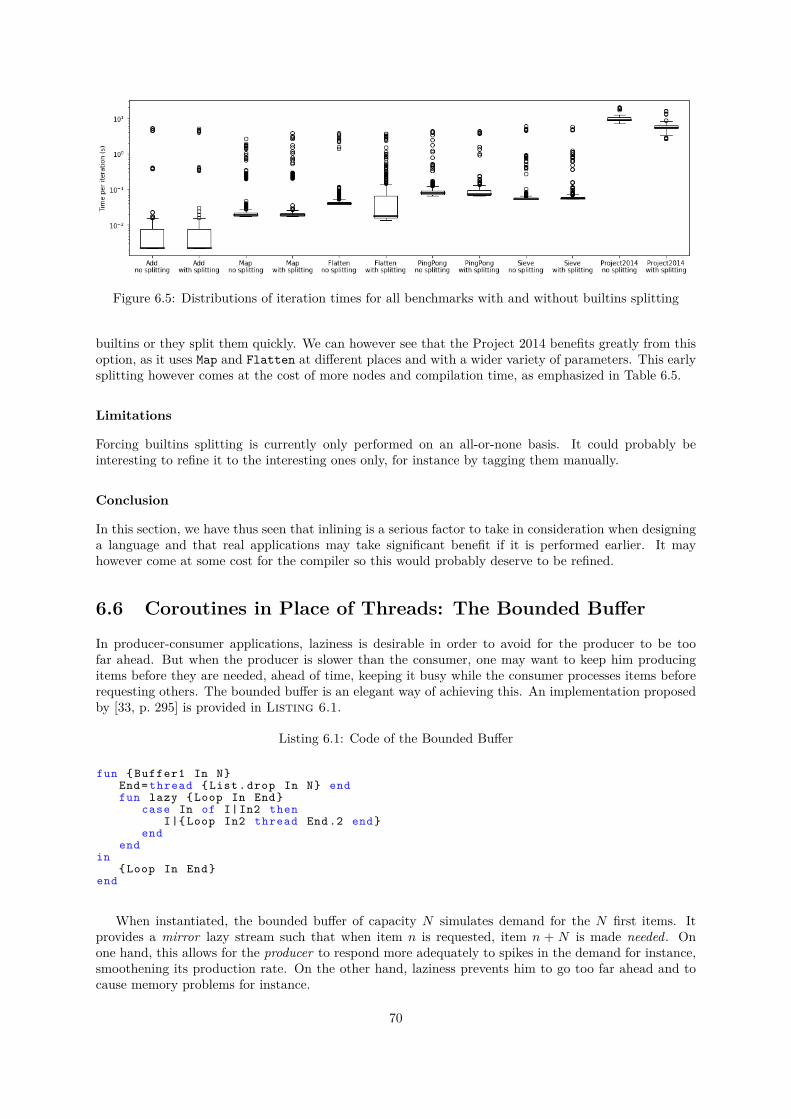
Figure 6.5: Distributions of iteration times for all benchmarks with and without builtins splitting
builtins or they split them quickly. We can however see that the Project 2014 benefits greatly from thisoption, as it uses Map and Flatten at different places and with a wider variety of parameters. This earlysplitting however comes at the cost of more nodes and compilation time, as emphasized in Table 6.5.
Limitations
Forcing builtins splitting is currently only performed on an all-or-none basis. It could probably beinteresting to refine it to the interesting ones only, for instance by tagging them manually.
Conclusion
In this section, we have thus seen that inlining is a serious factor to take in consideration when designinga language and that real applications may take significant benefit if it is performed earlier. It mayhowever come at some cost for the compiler so this would probably deserve to be refined.
6.6 Coroutines in Place of Threads: The Bounded Buffer
In producer-consumer applications, laziness is desirable in order to avoid for the producer to be toofar ahead. But when the producer is slower than the consumer, one may want to keep him producingitems before they are needed, ahead of time, keeping it busy while the consumer processes items beforerequesting others. The bounded buffer is an elegant way of achieving this. An implementation proposedby [33, p. 295] is provided in Listing 6.1.
Listing 6.1: Code of the Bounded Buffer
fun { Buffer1 In N}End= thread {List.drop In N} endfun lazy {Loop In End}
case In of I|In2 thenI|{ Loop In2 thread End .2 end}
endend
in{Loop In End}
end
When instantiated, the bounded buffer of capacity N simulates demand for the N first items. Itprovides a mirror lazy stream such that when item n is requested, item n + N is made needed. Onone hand, this allows for the producer to respond more adequately to spikes in the demand for instance,smoothening its production rate. On the other hand, laziness prevents him to go too far ahead and tocause memory problems for instance.
70
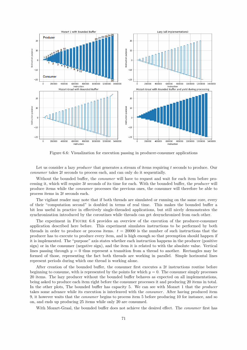
Figure 6.6: Visualization for execution passing in producer-consumer applications
Let us consider a lazy producer that generates a stream of items requiring t seconds to produce. Ourconsumer takes 2t seconds to process each, and can only do it sequentially.
Without the bounded buffer, the consumer will have to request and wait for each item before pro-cessing it, which will require 3t seconds of its time for each. With the bounded buffer, the producer willproduce items while the consumer processes the previous ones, the consumer will therefore be able toprocess items in 2t seconds each.
The vigilant reader may note that if both threads are simulated or running on the same core, everyof their “computation second” is doubled in terms of real time. This makes the bounded buffer abit less useful in practice in effectively single-threaded applications, but still nicely demonstrates thesynchronization introduced by the coroutines while threads can get desynchronized from each other.
The experiment in Figure 6.6 provides an overview of the execution of the producer-consumerapplication described here before. This experiment simulates instructions to be performed by boththreads in order to produce or process items. t = 20000 is the number of such instructions that theproducer has to execute to produce every item, and is high enough so that preemption should happen ifit is implemented. The “purpose” axis states whether each instruction happens in the producer (positivesign) or in the consumer (negative sign), and the item it is related to with the absolute value. Verticallines passing through y = 0 thus represent a transition from a thread to another. Rectangles may beformed of those, representing the fact both threads are working in parallel. Simple horizontal linesrepresent periods during which one thread is working alone.
After creation of the bounded buffer, the consumer first executes a 2t instructions routine beforebeginning to consume, with is represented by the points for which y = 0. The consumer simply processes20 items. The lazy producer without the bounded buffer behaves as expected on all implementations,being asked to produce each item right before the consumer processes it and producing 20 items in total.In the other plots, The bounded buffer has capacity 5. We can see with Mozart 1 that the producertakes some advance while its execution is interleaved with the consumer . After having produced item9, it however waits that the consumer begins to process item 5 before producing 10 for instance, and soon, and ends up producing 25 items while only 20 are consumed.
With Mozart-Graal, the bounded buffer does not achieve the desired effect. The consumer first has
71
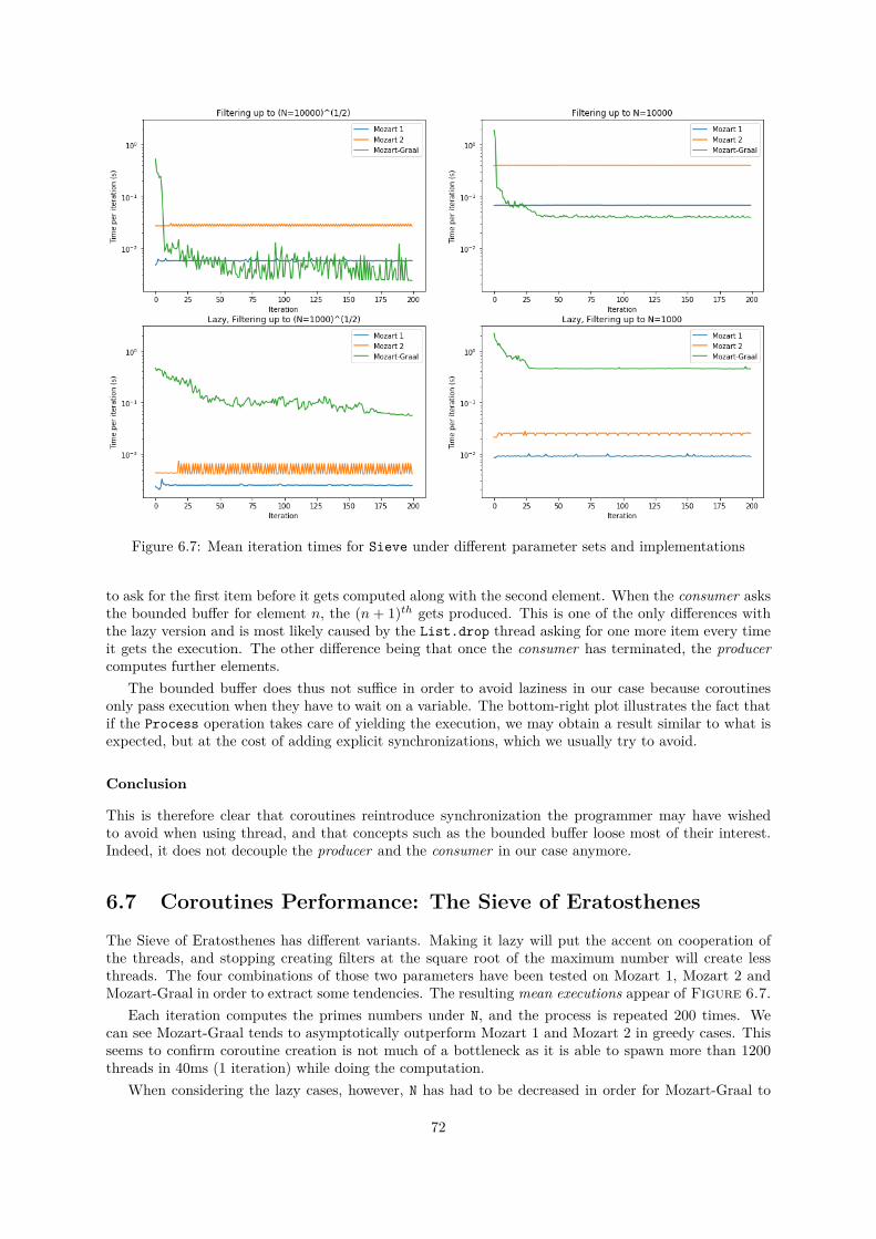
Figure 6.7: Mean iteration times for Sieve under different parameter sets and implementations
to ask for the first item before it gets computed along with the second element. When the consumer asksthe bounded buffer for element n, the (n + 1)th gets produced. This is one of the only differences withthe lazy version and is most likely caused by the List.drop thread asking for one more item every timeit gets the execution. The other difference being that once the consumer has terminated, the producercomputes further elements.
The bounded buffer does thus not suffice in order to avoid laziness in our case because coroutinesonly pass execution when they have to wait on a variable. The bottom-right plot illustrates the fact thatif the Process operation takes care of yielding the execution, we may obtain a result similar to what isexpected, but at the cost of adding explicit synchronizations, which we usually try to avoid.
Conclusion
This is therefore clear that coroutines reintroduce synchronization the programmer may have wishedto avoid when using thread, and that concepts such as the bounded buffer loose most of their interest.Indeed, it does not decouple the producer and the consumer in our case anymore.
6.7 Coroutines Performance: The Sieve of Eratosthenes
The Sieve of Eratosthenes has different variants. Making it lazy will put the accent on cooperation ofthe threads, and stopping creating filters at the square root of the maximum number will create lessthreads. The four combinations of those two parameters have been tested on Mozart 1, Mozart 2 andMozart-Graal in order to extract some tendencies. The resulting mean executions appear of Figure 6.7.
Each iteration computes the primes numbers under N, and the process is repeated 200 times. Wecan see Mozart-Graal tends to asymptotically outperform Mozart 1 and Mozart 2 in greedy cases. Thisseems to confirm coroutine creation is not much of a bottleneck as it is able to spawn more than 1200threads in 40ms (1 iteration) while doing the computation.
When considering the lazy cases, however, N has had to be decreased in order for Mozart-Graal to
72
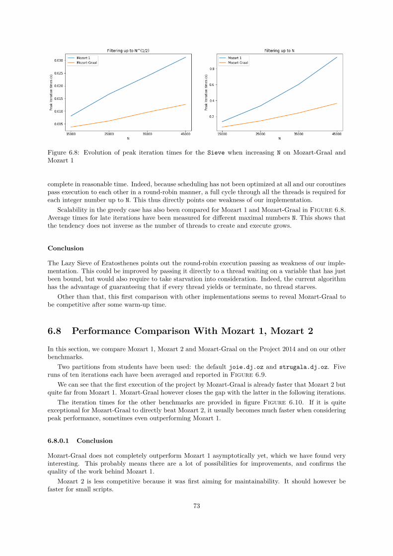
Figure 6.8: Evolution of peak iteration times for the Sieve when increasing N on Mozart-Graal andMozart 1
complete in reasonable time. Indeed, because scheduling has not been optimized at all and our coroutinespass execution to each other in a round-robin manner, a full cycle through all the threads is required foreach integer number up to N. This thus directly points one weakness of our implementation.
Scalability in the greedy case has also been compared for Mozart 1 and Mozart-Graal in Figure 6.8.Average times for late iterations have been measured for different maximal numbers N. This shows thatthe tendency does not inverse as the number of threads to create and execute grows.
Conclusion
The Lazy Sieve of Eratosthenes points out the round-robin execution passing as weakness of our imple-mentation. This could be improved by passing it directly to a thread waiting on a variable that has justbeen bound, but would also require to take starvation into consideration. Indeed, the current algorithmhas the advantage of guaranteeing that if every thread yields or terminate, no thread starves.
Other than that, this first comparison with other implementations seems to reveal Mozart-Graal tobe competitive after some warm-up time.
6.8 Performance Comparison With Mozart 1, Mozart 2
In this section, we compare Mozart 1, Mozart 2 and Mozart-Graal on the Project 2014 and on our otherbenchmarks.
Two partitions from students have been used: the default joie.dj.oz and strugala.dj.oz. Fiveruns of ten iterations each have been averaged and reported in Figure 6.9.
We can see that the first execution of the project by Mozart-Graal is already faster that Mozart 2 butquite far from Mozart 1. Mozart-Graal however closes the gap with the latter in the following iterations.
The iteration times for the other benchmarks are provided in figure Figure 6.10. If it is quiteexceptional for Mozart-Graal to directly beat Mozart 2, it usually becomes much faster when consideringpeak performance, sometimes even outperforming Mozart 1.
6.8.0.1 Conclusion
Mozart-Graal does not completely outperform Mozart 1 asymptotically yet, which we have found veryinteresting. This probably means there are a lot of possibilities for improvements, and confirms thequality of the work behind Mozart 1.
Mozart 2 is less competitive because it was first aiming for maintainability. It should however befaster for small scripts.
73
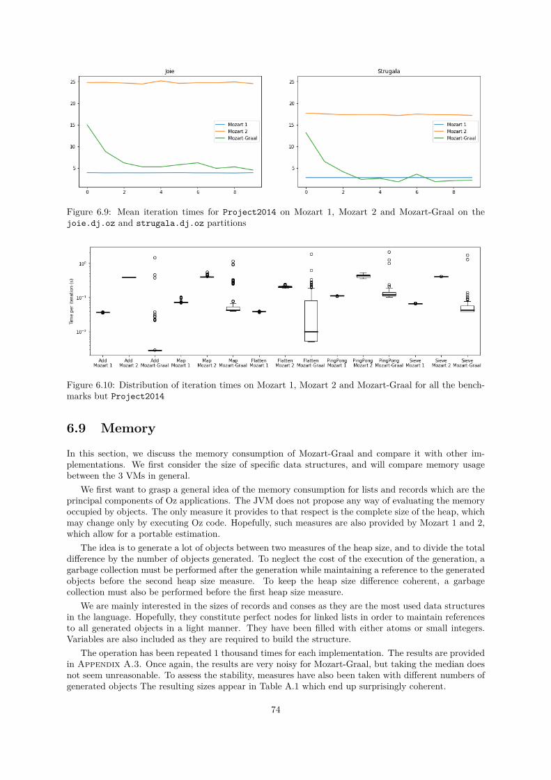
Figure 6.9: Mean iteration times for Project2014 on Mozart 1, Mozart 2 and Mozart-Graal on thejoie.dj.oz and strugala.dj.oz partitions
Figure 6.10: Distribution of iteration times on Mozart 1, Mozart 2 and Mozart-Graal for all the bench-marks but Project2014
6.9 Memory
In this section, we discuss the memory consumption of Mozart-Graal and compare it with other im-plementations. We first consider the size of specific data structures, and will compare memory usagebetween the 3 VMs in general.
We first want to grasp a general idea of the memory consumption for lists and records which are theprincipal components of Oz applications. The JVM does not propose any way of evaluating the memoryoccupied by objects. The only measure it provides to that respect is the complete size of the heap, whichmay change only by executing Oz code. Hopefully, such measures are also provided by Mozart 1 and 2,which allow for a portable estimation.
The idea is to generate a lot of objects between two measures of the heap size, and to divide the totaldifference by the number of objects generated. To neglect the cost of the execution of the generation, agarbage collection must be performed after the generation while maintaining a reference to the generatedobjects before the second heap size measure. To keep the heap size difference coherent, a garbagecollection must also be performed before the first heap size measure.
We are mainly interested in the sizes of records and conses as they are the most used data structuresin the language. Hopefully, they constitute perfect nodes for linked lists in order to maintain referencesto all generated objects in a light manner. They have been filled with either atoms or small integers.Variables are also included as they are required to build the structure.
The operation has been repeated 1 thousand times for each implementation. The results are providedin Appendix A.3. Once again, the results are very noisy for Mozart-Graal, but taking the median doesnot seem unreasonable. To assess the stability, measures have also been taken with different numbers ofgenerated objects The resulting sizes appear in Table A.1 which end up surprisingly coherent.
74
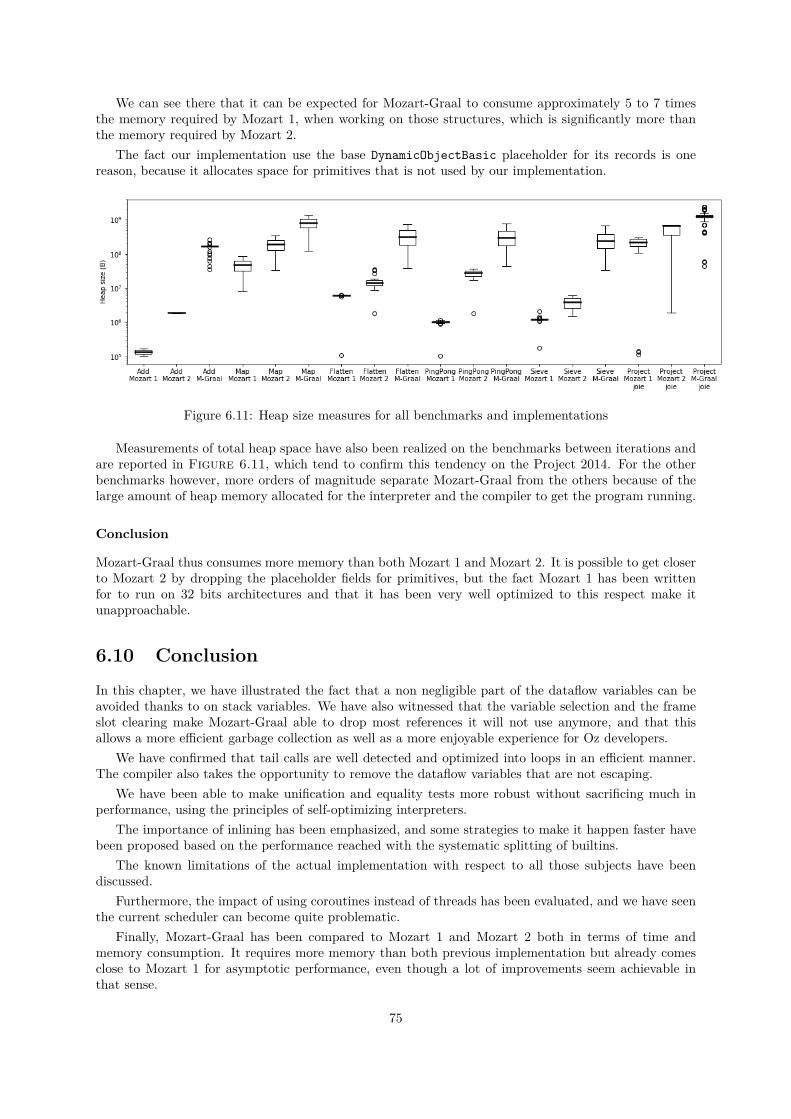
We can see there that it can be expected for Mozart-Graal to consume approximately 5 to 7 timesthe memory required by Mozart 1, when working on those structures, which is significantly more thanthe memory required by Mozart 2.
The fact our implementation use the base DynamicObjectBasic placeholder for its records is onereason, because it allocates space for primitives that is not used by our implementation.
Figure 6.11: Heap size measures for all benchmarks and implementations
Measurements of total heap space have also been realized on the benchmarks between iterations andare reported in Figure 6.11, which tend to confirm this tendency on the Project 2014. For the otherbenchmarks however, more orders of magnitude separate Mozart-Graal from the others because of thelarge amount of heap memory allocated for the interpreter and the compiler to get the program running.
Conclusion
Mozart-Graal thus consumes more memory than both Mozart 1 and Mozart 2. It is possible to get closerto Mozart 2 by dropping the placeholder fields for primitives, but the fact Mozart 1 has been writtenfor to run on 32 bits architectures and that it has been very well optimized to this respect make itunapproachable.
6.10 Conclusion
In this chapter, we have illustrated the fact that a non negligible part of the dataflow variables can beavoided thanks to on stack variables. We have also witnessed that the variable selection and the frameslot clearing make Mozart-Graal able to drop most references it will not use anymore, and that thisallows a more efficient garbage collection as well as a more enjoyable experience for Oz developers.
We have confirmed that tail calls are well detected and optimized into loops in an efficient manner.The compiler also takes the opportunity to remove the dataflow variables that are not escaping.
We have been able to make unification and equality tests more robust without sacrificing much inperformance, using the principles of self-optimizing interpreters.
The importance of inlining has been emphasized, and some strategies to make it happen faster havebeen proposed based on the performance reached with the systematic splitting of builtins.
The known limitations of the actual implementation with respect to all those subjects have beendiscussed.
Furthermore, the impact of using coroutines instead of threads has been evaluated, and we have seenthe current scheduler can become quite problematic.
Finally, Mozart-Graal has been compared to Mozart 1 and Mozart 2 both in terms of time andmemory consumption. It requires more memory than both previous implementation but already comesclose to Mozart 1 for asymptotic performance, even though a lot of improvements seem achievable inthat sense.
75

76
Chapter 7
Future Work
Union-Find for Testing Whether Two Variables are Equivalent
In Section 4.1, the circular list of variables has been introduced as very practical for ensuring O(1)queries on dataflow variables. However, linking two unbound variables requires to test whether both arealready linked or not in order to avoid breaking the circular list. This test currently makes a full passon one list, hence having complexity O(n), n being the size of the biggest equivalence set of both.
This potentially provides creating a set of n equivalent variables a complexity of O(n2). If pathologicalcases are rare in practice, using the Union-Find for this test would simply solve the complexity problemwhile keeping the advantages of the other for queries.
This algorithm could even used in the case of large sets only, to avoid the cost of recursion while setsare small.
Improving Threads
We have seen in Section 6.7 that scheduling in Mozart-Graal is currently far from perfect. Indeed,yielding the execution from a coroutine and coming back to it has linear complexity in the total numberof coroutines, even in the case where all other coroutines are waiting on a variable. Optimizing thescheduling, for instance by considering coroutines waiting on just-bound variables, would be a simpleimprovement. Starvation should ideally be taken in consideration.
Some preemption mechanism could also be added, making the coroutines closer to the authentic Ozthreads. This would however require checks to be put in the program in order to prevent routines frombeing to run indefinitely, which will of course affect performance.
Finally, Mozart-Graal does not currently take advantage of multiple cores for Oz programs. Thelanguage could probably be extended to take advantage from them, as it has been made for the Mozart 2implementation [45].
Broader Variable Optimization Around Call Expressions
For now, call expressions are only optimized when they are explicit tail calls. It would be interestingto apply the technique from Section 4.4.3 to any call expression that ends up being unified with adeclared variable. This would as well generalize the tail call detection for all procedures.
Improve Support for Unboxed Primitives
Until now, primitives are only unboxed when stored into stack frames. Values flowing through thegraph are not, which implies a lot of boxing and unboxing operations in interpreter mode and couldbe optimized thanks to the ideas from [20]. The Truffle DynamicObjects also have support for storingprimitives, but would require to be more careful when comparing shapes for instance.
77
Smarter Frame Slot Clearing
For now, there are two ideas coming along with Section 5.1.3.The first is that it would be feasible for thread or lock procedures to clear their environment slots as
it is done for local variables everywhere. Because anonymous procedures created by this syntactic sugarare guaranteed to be called only once after their declaration, it would be correct for the static analysisto tag the slots from the external environment as well.
The second idea is that it should be possible to economize nodes performing the slots clearing (i.e.ResetSlotNodes). Either because the procedure could be guaranteed to terminate quickly after (onlyunifications happen after for instance), or because some several ResetSlotNodes could be merged whenonly separated by quick operations.
Experimenting With More Dynamic Optimizations
A lot of directions have not been experimented yet. For instance, replacing bound variables by theirvalue on the stack when reading them or trying to dereference variables before performing calls.
Resugaring Oz Kernel Language
Currently, Mozart-Graal takes advantage from the way natural code is written. Detecting self tail callsrelies on the name procedures are declared with (before being desugared into a unification), nestedexpressions directly reduce the need for frame slots. One-time procedures would also most likely bedetected when desugared.
The idea is that the Oz kernel language that is very good for bytecode VMs is a bit too low level forMozart-Graal, so it will render a different and less optimized AST than the human version. It would begreat to achieve close equivalence.
Two approaches are therefore possible: Either take the Oz kernel code and generate more human-likecode, basically trying to reverse the desugaring, or refine those passes of the static analysis.
Interoperability With the JVM Ecosystem
Allowing Oz to interoperate with existing Java libraries could make Oz applications benefit from featuresfor which no specific builtin would have to be maintained.
Truffle provides its PolyglotEngine for interoperability with Java but also other languages developedon it. Being compliant with it would thus means all of them can be accessed from Oz and that Oz couldexpose some of its mechanisms to them.
Making use of the Oz Compiler
For now, Mozart-Graal uses Mozart 2’s bootcompiler parser. If this works well for the main features ofthe language, some syntactic constructs encountered here and there are not recognized. In order to avoidduplicating work and to stay in the spirit of previous implementations, the Oz compiler could handleprograms down to the Oz kernel language AST or some intermediate, and rely on some other tool toconvert it into a Truffle AST.
78
Chapter 8
Conclusion
This dissertation aimed at discussing Mozart-Graal on its way to become an efficient Oz implementationon Truffle and Graal, while evaluating if the features they propose would suffice to achieve it.
In Chapter 2, we have discussed the main concepts behind self-optimizing AST interpreters and howTruffle provides a convenient way of implementing them. We have also understood in what it constitutesa front-end to the Graal compiler, which is able to recognize and optimize them optimistically. We haveseen the basic ideas behind their orchestration to compile dynamic languages efficiently.
In Chapter 3, we have exposed the architecture of Mozart-Graal and have defined its main char-acteristics. Indeed, we wanted the implemented language to be as close as possible to Oz, up to somelimitations such as the quantity of implemented builtins and the concurrency model for threads that isnot matched in our case. We have also seen that Mozart-Graal is based on Mozart 2 for the parsing andsome parts of the static analysis, the standard library and the tests.
In Chapter 4, we have transposed the key Oz concepts to our interpreter. We have seen how thevariables, the dataflow, the environment, the procedures, the different primitive data structures as well asthe unification, equality testing, pattern matching and the tail call optimization can be implemented whenperformance is not a requirement. We have acknowledged the Truffle framework proposes interestingprimitives to implement the environment, the procedures, the records and the tail calls, and that its DSLallows to build a system that is easy to reason about.
Chapter 5 has provided improvements in memory usage and performance. First by refining staticanalysis in order to particularize self tail calls, to avoid indirection for particular cases of declaredvariables and for releasing references in the stack frames as soon as possible. We have then annotatedthe interpreter for the compiler to be able to focus on the interesting parts of programs, to performinlining and to optimize the control flow of tail calls. Furthermore, ways to make those optimizationoccur faster such as OSR and builtins splitting have been explored. Finally, efficient specializations forunification and equality tests have been proposed.
In Chapter 6, we have attested that part of the dataflow variables can be avoided thanks to therefinements of the static analysis and that this way of implementing the environment and of clearingthe slots allows more efficient garbage collections and makes the language less difficult to reason aboutwhen it comes to reference retention. We have also confirmed that the Graal compiler takes care oftransforming tail calls into loops when possible, and that it removes the overhead of variables that arenot escaping from compilation units. We have confirmed that efficient specializations for unification andequality tests bring a significant performance gain in contrast to the general mechanism.
The role of inlining in the general performance has been emphasized, and significant improvementshave been obtained with OSR and the builtins splitting. Mozart-Graal has been proved to consume morememory than Mozart 1 and Mozart 2 but could close the gap with Mozart 2. It also seems to have thepotential to outperform Mozart 1 on long executions and Mozart 2 on shorter ones. The supplementarysynchronization introduced by using coroutines instead of threads has also been illustrated.
Finally, the current limitations of the implementation have been discussed. We propose furtherdevelopments and are rather confident that with them and the active research made on Truffle andGraal, Mozart-Graal could become a viable option for running all kinds of Oz applications.
79

80
Bibliography
[1] Java (programming language). https://en.wikipedia.org/wiki/Java_(programming_language). 17
[2] Java Virtual Machine. https://en.wikipedia.org/wiki/Java_virtual_machine. 17
[3] The Python Programming Language. https://www.python.org/. 17
[4] Jython: Python for the Java Platform. http://www.jython.org/. 17
[5] Ruby Programming Language. https://www.ruby-lang.org/. 17
[6] The Ruby Programming Language on the JVM. http://jruby.org/. 17
[7] Charles Nutter. JRuby: The Pain of Bringing an Off-Platform Dynamic Language to the JVM,2009. https://www.infoq.com/presentations/nutter-jruby-jvm-lang-summit. 17
[8] Charles Nutter. A First Taste of InvokeDynamic, 2008. http://blog.headius.com/2008/09/first-taste-of-invokedynamic.html. 17
[9] OpenJDK. The Da Vinci Machine Project. http://openjdk.java.net/projects/mlvm/. 17
[10] Oracle. GraalVM - New JIT Compiler and Polyglot Runtime for the JVM. http://www.oracle.com/technetwork/oracle-labs/program-languages/overview/index-2301583.html. 17
[11] Chris Seaton. Ruby Benchmarks Report. http://chrisseaton.com/rubytruffle/deoptimizing/benchmarks. 17
[12] Chrome V8. https://developers.google.com/v8/. 17
[13] Stefan Marr, Benoit Daloze, and Hanspeter Mössenböck. Cross-language compiler benchmarking:Are we fast yet? SIGPLAN Not., 52(2):120–131, November 2016. 17
[14] Oz Programming Language. https://en.wikipedia.org/wiki/Oz_(programming_language). 17
[15] The Mozart Programming System. http://mozart.github.io/. 17
[16] Benoit Daloze. Mozart-Graal repository. https://github.com/eregon/mozart-graal. 17, 18
[17] Modifications to Mozart-Graal. https://github.com/mistasse/mozart-graal/tree/memoire-final. 18
[18] Maxime Istasse. Mozart-Graal Benchmarking repository. https://github.com/mistasse/mozart-graal-benchmarking/tree/memoire-final. 18, 30, 61, 63, 85
[19] Project Jupyter. http://jupyter.org/. 18, 61
[20] Thomas Würthinger, Andreas Wöß, Lukas Stadler, Gilles Duboscq, Doug Simon, and ChristianWimmer. Self-optimizing ast interpreters. In Proceedings of the 8th Symposium on Dynamic Lan-guages, DLS ’12, pages 73–82, New York, NY, USA, 2012. ACM. 20, 77
81
[21] Christian Humer, Christian Wimmer, Christian Wirth, Andreas Wöß, and Thomas Würthinger. Adomain-specific language for building self-optimizing ast interpreters. In Proceedings of the 2014International Conference on Generative Programming: Concepts and Experiences, GPCE 2014,pages 123–132, New York, NY, USA, 2014. ACM. 21
[22] HotSpot. https://en.wikipedia.org/wiki/HotSpot. 22
[23] Lukas Stadler, Thomas Würthinger, and Hanspeter Mössenböck. Partial escape analysis and scalarreplacement for java. In Proceedings of Annual IEEE/ACM International Symposium on CodeGeneration and Optimization, CGO ’14, pages 165:165–165:174, New York, NY, USA, 2014. ACM.22, 23
[24] Gilles Duboscq, Lukas Stadler, Thomas Würthinger, Doug Simon, Christian Wimmer, andHanspeter Mössenböck. Graal ir: An extensible declarative intermediate representation. 22, 62
[25] Static single assignment form. https://en.wikipedia.org/wiki/Static_single_assignment_form. 22
[26] Cliff Click. Global code motion/global value numbering. In Proceedings of the ACM SIGPLAN 1995Conference on Programming Language Design and Implementation, PLDI ’95, pages 246–257, NewYork, NY, USA, 1995. ACM. 23
[27] Oracle. Java HotSpotTM Virtual Machine Performance Enhancements. http://docs.oracle.com/javase/7/docs/technotes/guides/vm/performance-enhancements-7.html. 23
[28] Gilles Duboscq, Thomas Würthinger, Lukas Stadler, Christian Wimmer, Doug Simon, andHanspeter Mössenböck. An intermediate representation for speculative optimizations in a dynamiccompiler. In Proceedings of the 7th ACM Workshop on Virtual Machines and Intermediate Lan-guages, VMIL ’13, pages 1–10, New York, NY, USA, 2013. ACM. 24
[29] Mozart Documentation. http://mozart.github.io/mozart-v1/doc-1.4.0/. 25
[30] Building the JVMCI for Mozart-Graal. https://github.com/eregon/mozart-graal/tree/master/vm/jvmci. 25
[31] Scala Programming Language. https://en.wikipedia.org/wiki/Scala_(programming_language). 25
[32] Guillaume Maudoux. Projet Dj’OZ, 2014. http://perso.uclouvain.be/guillaume.maudoux/dewplayer/. 26, 61, 65
[33] Peter Van Roy and Seif Haridi. Concepts, Techniques, and Models of Computer Programming. TheMIT Press, 1st edition, 2004. 27, 37, 41, 45, 70
[34] Ana Lûcia De Moura and Roberto Ierusalimschy. Revisiting coroutines. 2004. 27
[35] Charles Nutter. JRuby - The Hard Parts. https://www.slideshare.net/CharlesNutter/jruby-the-hard-parts. 28
[36] Akka. http://akka.io/. 28
[37] Parallel Universe. Quasar. http://www.paralleluniverse.co/quasar/. 28
[38] Parallel Universe. Implementing, Abstracting and Benchmarking Lightweight Threads on the JVM,2014. http://blog.paralleluniverse.co/2014/02/06/fibers-threads-strands/. 28
[39] Lukas Stadler, Thomas Würthinger, and Christian Wimmer. Efficient coroutines for the java plat-form. In Proceedings of the 8th International Conference on the Principles and Practice of Program-ming in Java, PPPJ ’10, pages 20–28, New York, NY, USA, 2010. ACM. 28
[40] Disjoint-set data structure. https://en.wikipedia.org/wiki/Disjoint-set_data_structure.30
82
[41] Andreas Wöß, Christian Wirth, Daniele Bonetta, Chris Seaton, Christian Humer, and HanspeterMössenböck. An object storage model for the truffle language implementation framework. In Pro-ceedings of the 2014 International Conference on Principles and Practices of Programming on theJava platform: Virtual machines, Languages, and Tools, pages 133–144. ACM, 2014. 38
[42] Fredrik Skeel Løkke. Scala and Design Patterns-exploring Language Expressivity. Aarhus Univer-sitet, Datalogisk Institut, 2009. 44
[43] SSW JKU. Ideal Graph Visualizer. http://ssw.jku.at/General/Staff/TW/igv.html. 62
[44] Kevin Menard. A Systematic Approach to Improving Truf-fleRuby Performance, 2017. http://nirvdrum.com/2017/05/30/a-systematic-approach-to-improving-truffleruby-performance.html. 62
[45] Benoit Daloze, Peter Van Roy, Per Brand, and Sébastien Doeraene. Extending Mozart 2 to supportmulticore processors, 2014. 77
83

84
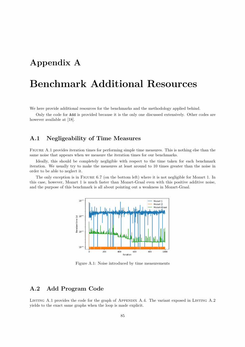
Appendix A
Benchmark Additional Resources
We here provide additional resources for the benchmarks and the methodology applied behind.Only the code for Add is provided because it is the only one discussed extensively. Other codes are
however available at [18].
A.1 Negligeability of Time Measures
Figure A.1 provides iteration times for performing simple time measures. This is nothing else than thesame noise that appears when we measure the iteration times for our benchmarks.
Ideally, this should be completely negligible with respect to the time taken for each benchmarkiteration. We usually try to make the measures at least around to 10 times greater than the noise inorder to be able to neglect it.
The only exception is in Figure 6.7 (on the bottom left) where it is not negligible for Mozart 1. Inthis case, however, Mozart 1 is much faster than Mozart-Graal even with this positive additive noise,and the purpose of this benchmark is all about pointing out a weakness in Mozart-Graal.
Figure A.1: Noise introduced by time measurements
A.2 Add Program Code
Listing A.1 provides the code for the graph of Appendix A.4. The variant exposed in Listing A.2yields to the exact same graphs when the loop is made explicit.
85
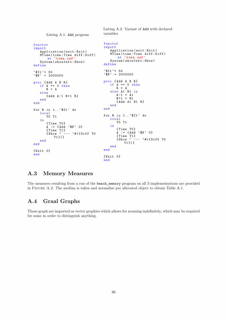
Listing A.1: Add program
functorimport
Application (exit:Exit)MTime(time:Time diff:Diff)
at ’time.ozf ’System ( showInfo :Show)
define
‘$It ‘= 50‘$N ‘ = 2000000
proc {Add A B R}if A == 0 then
R = Aelse
{Add A-1 B+1 R}end
end
for R in 1..‘$It ‘ dolocal
T0 T1in
{Time T0}A := {Add ‘$N ‘ 0}{Time T1}{Show " --- "#({ Diff T0
T1})}end
end
{Exit 0}end
Listing A.2: Variant of Add with declaredvariables
functorimport
Application (exit:Exit)MTime(time:Time diff:Diff)
at ’time.ozf ’System ( showInfo :Show)
define
‘$It ‘= 50‘$N ‘ = 2000000
proc {Add A B R}if A == 0 then
R = Aelse A1 B1 in
A-1 = A1B+1 = B1{Add A1 B1 R}
endend
for R in 1..‘$It ‘ dolocal
T0 T1in
{Time T0}A := {Add ‘$N ‘ 0}{Time T1}{Show " --- "#({ Diff T0
T1})}end
end
{Exit 0}end
A.3 Memory Measures
The measures resulting from a run of the bench_memory program on all 3 implementations are providedin Figure A.2. The median is taken and normalize per allocated object to obtain Table A.1.
A.4 Graal Graphs
Those graph are imported as vector graphics which allows for zooming indefinitely, which may be requiredfor some in order to distinguish anything.
86
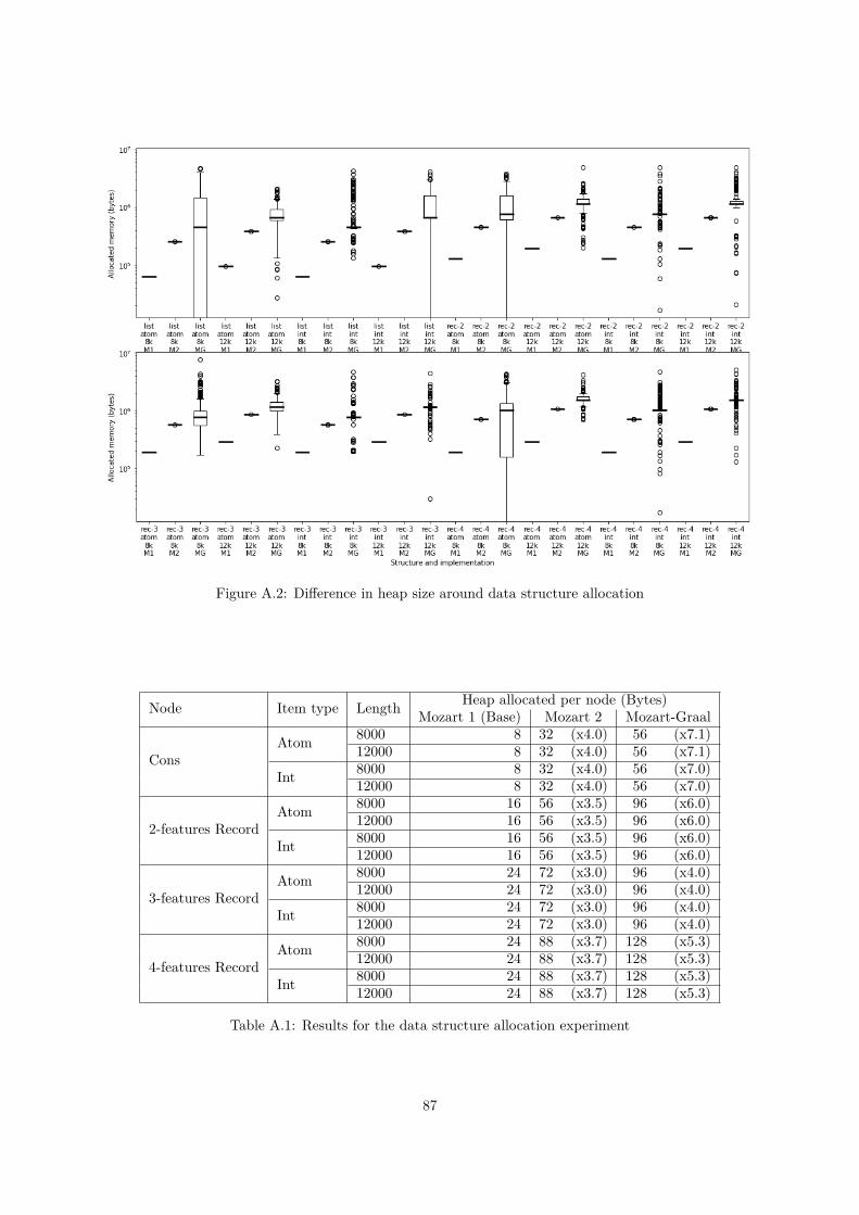
Figure A.2: Difference in heap size around data structure allocation
Node Item type Length Heap allocated per node (Bytes)Mozart 1 (Base) Mozart 2 Mozart-Graal
ConsAtom 8000 8 32 (x4.0) 56 (x7.1)
12000 8 32 (x4.0) 56 (x7.1)
Int 8000 8 32 (x4.0) 56 (x7.0)12000 8 32 (x4.0) 56 (x7.0)
2-features RecordAtom 8000 16 56 (x3.5) 96 (x6.0)
12000 16 56 (x3.5) 96 (x6.0)
Int 8000 16 56 (x3.5) 96 (x6.0)12000 16 56 (x3.5) 96 (x6.0)
3-features RecordAtom 8000 24 72 (x3.0) 96 (x4.0)
12000 24 72 (x3.0) 96 (x4.0)
Int 8000 24 72 (x3.0) 96 (x4.0)12000 24 72 (x3.0) 96 (x4.0)
4-features RecordAtom 8000 24 88 (x3.7) 128 (x5.3)
12000 24 88 (x3.7) 128 (x5.3)
Int 8000 24 88 (x3.7) 128 (x5.3)12000 24 88 (x3.7) 128 (x5.3)
Table A.1: Results for the data structure allocation experiment
87
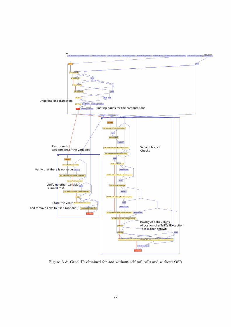
Unboxing of parameters
First branch:
Assignment of the variablesSecond branch:
Checks
Boxing of both values,
Allocation of a TailCallException
That is then thrown
Floating nodes for the computations
Verify that there is no value
Verify no other variable
is linked to it
Store the value
And remove links to itself (optional)
Figure A.3: Graal IR obtained for Add without self tail calls and without OSR
88
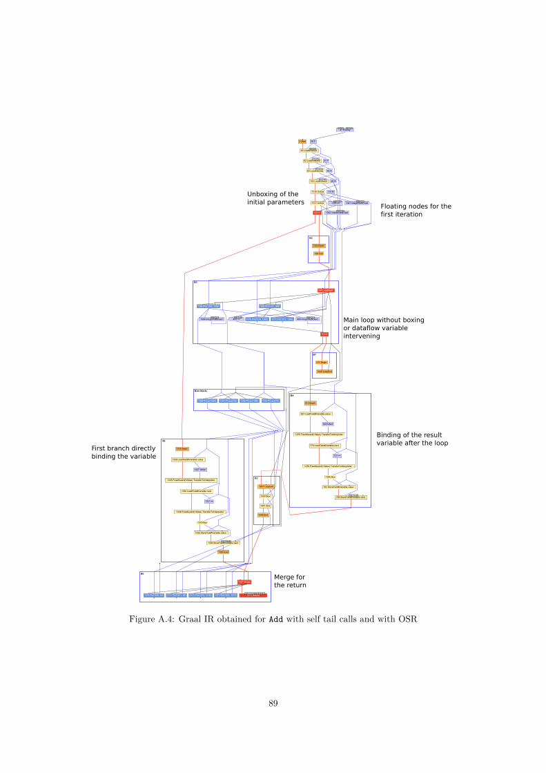
First branch directly
binding the variable
Main loop without boxing
or dataflow variable
intervening
Binding of the result
variable after the loop
Unboxing of the
initial parametersFloating nodes for the
first iteration
Merge for
the return
Figure A.4: Graal IR obtained for Add with self tail calls and with OSR
89
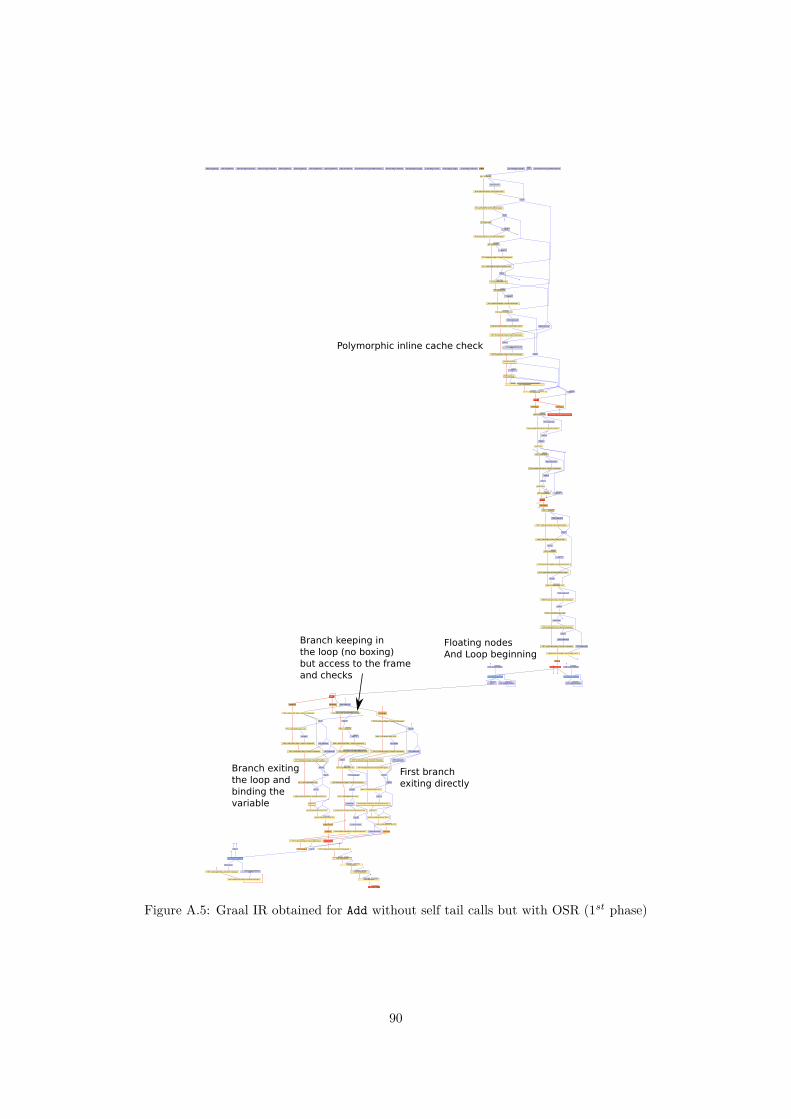
Polymorphic inline cache check
Floating nodes
And Loop beginning
Branch exiting
the loop and
binding the
variable
First branch
exiting directly
Branch keeping in
the loop (no boxing)
but access to the frame
and checks
Figure A.5: Graal IR obtained for Add without self tail calls but with OSR (1st phase)
90
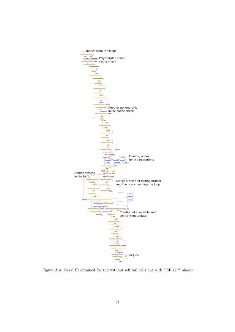
Polymorphic inline
cache check
... (nodes from the loop)
Another polymorphic
inline cache check
Floating nodes
for the operations
Branch staying
in the loop
Merge of the first exiting branch
and the branch exiting the loop
Creation of a variable and
cell content update
{Time} call
Figure A.6: Graal IR obtained for Add without self tail calls but with OSR (2nd phase)
91

92
Appendix B
Known bugs
• Linking an unbound variable to a view on an unbound variable makes it possible to write throughthe view.
• Open patterns like ’|’(X Y ...) would not match OzCons
• A = rec(1 A.1) does not bind A before evaluating A.1. The coroutine therefore yields indefinitely.
93

94
Rue Archimède, 1 bte L6.11.01, 1348 Louvain-la-Neuve www.uclouvain.be/epl