August 2010 Doc ID 17353 Rev 1 1/34

AN3192Application note

Using LSM303DLH for a tilt compensated electronic compass

IntroductionThis application note describes the method for building a tilt compensated electronic compass using an LSM303DLH sensor module.

The LSM303DLH is a 5 x 5 x 1 mm with LGA-28L package IC chip that includes a 3D digital linear acceleration and a 3D digital magnetic sensor. It has a selectable linear acceleration full scale range of ±2g / ±4g / ±8g and a selectable magnetic field full scale range of ±1.3 / ±1.9 / ±2.5 / ±4.0 / ±4.7 / ±5.6 / ±8.1 gauss. Both the magnetic sensor and the accelerometer parts can be powered down separately to reduce power consumption. Sensor measurements can be acquired by a microcontroller through an I2C serial bus interface.

The key features of the system are:

■ One single chip solution

■ I2C communication interface

■ Tilt compensation

Section 1 describes the basics of the electronic compass. Section 2 presents a typical hardware connection between the LSM303DLH and a microcontroller and sample code for sensor data acquisition. Section 3 focuses on the methods of the determination of sensor calibration parameters. Section 4 shows the methods of lab testing and field testing for checking the electronic compass performance. Section 5 gives recommendations for microcontroller firmware implementation when designing a standalone tilt compensated electronic compass.

www.st.com

Contents AN3192

2/34 Doc ID 17353 Rev 1

Contents

1 Electronic compass basics . . . . . . . . . . . . . . . . . . . . . . . . . . . . . . . . . . . 5

1.1 Definitions . . . . . . . . . . . . . . . . . . . . . . . . . . . . . . . . . . . . . . . . . . . . . . . . . . 5

1.2 Heading calculation . . . . . . . . . . . . . . . . . . . . . . . . . . . . . . . . . . . . . . . . . . 6

1.3 Tilt compensation . . . . . . . . . . . . . . . . . . . . . . . . . . . . . . . . . . . . . . . . . . . . 6

1.4 Electronic compass system . . . . . . . . . . . . . . . . . . . . . . . . . . . . . . . . . . . . 7

1.5 Getting started with LSM303DLH . . . . . . . . . . . . . . . . . . . . . . . . . . . . . . . . 8

2 LSM303DLH configuration . . . . . . . . . . . . . . . . . . . . . . . . . . . . . . . . . . . . 9

2.1 Typical hardware connection . . . . . . . . . . . . . . . . . . . . . . . . . . . . . . . . . . . 9

2.2 LSM303DLH accelerometer data acquisition . . . . . . . . . . . . . . . . . . . . . . . 9

2.3 LSM303DLH magnetic sensor data acquisition . . . . . . . . . . . . . . . . . . . . 10

3 Calibrating the LSM303DLH . . . . . . . . . . . . . . . . . . . . . . . . . . . . . . . . . . 12

3.1 LSM303DLH accelerometer calibration . . . . . . . . . . . . . . . . . . . . . . . . . . 12

3.2 LSM303DLH magnetic sensor calibration . . . . . . . . . . . . . . . . . . . . . . . . 12

3.2.1 Terminology . . . . . . . . . . . . . . . . . . . . . . . . . . . . . . . . . . . . . . . . . . . . . . 13

4 Testing the electronic compass . . . . . . . . . . . . . . . . . . . . . . . . . . . . . . . 15

4.1 Lab testing . . . . . . . . . . . . . . . . . . . . . . . . . . . . . . . . . . . . . . . . . . . . . . . . 15

4.1.1 Absolute heading testing . . . . . . . . . . . . . . . . . . . . . . . . . . . . . . . . . . . . 15

4.1.2 Tilt compensation testing . . . . . . . . . . . . . . . . . . . . . . . . . . . . . . . . . . . . 16

4.2 Field testing . . . . . . . . . . . . . . . . . . . . . . . . . . . . . . . . . . . . . . . . . . . . . . . 16

4.2.1 Relative heading testing . . . . . . . . . . . . . . . . . . . . . . . . . . . . . . . . . . . . . 17

4.2.2 Tilt compensation testing . . . . . . . . . . . . . . . . . . . . . . . . . . . . . . . . . . . . 17

5 Firmware implementation . . . . . . . . . . . . . . . . . . . . . . . . . . . . . . . . . . . . 18

Appendix A LSM303DLH pitch/roll/heading calculation . . . . . . . . . . . . . . . . . . . 19

A.1 Pitch/roll calculation. . . . . . . . . . . . . . . . . . . . . . . . . . . . . . . . . . . . . . . . . . 20

A.2 Heading calculation. . . . . . . . . . . . . . . . . . . . . . . . . . . . . . . . . . . . . . . . . . 22

Appendix B Accelerometer calibration method. . . . . . . . . . . . . . . . . . . . . . . . . . 24

AN3192 Contents

Doc ID 17353 Rev 1 3/34

Appendix C Magnetic sensor calibration method . . . . . . . . . . . . . . . . . . . . . . . . 27

C.1 Step 1: Soft-iron effect verification . . . . . . . . . . . . . . . . . . . . . . . . . . . . . . 27

C.2 Step 2: Hard-iron, soft-iron and scale factor compensation . . . . . . . . . . . 27

C.3 Step 3: Misalignment error compensation. . . . . . . . . . . . . . . . . . . . . . . . . 30

6 References . . . . . . . . . . . . . . . . . . . . . . . . . . . . . . . . . . . . . . . . . . . . . . . . 32

7 Revision history . . . . . . . . . . . . . . . . . . . . . . . . . . . . . . . . . . . . . . . . . . . 33

List of figures AN3192

4/34 Doc ID 17353 Rev 1

List of figures

Figure 1. Body coordinates and attitude angles. . . . . . . . . . . . . . . . . . . . . . . . . . . . . . . . . . . . . . . . . . 5Figure 2. Heading calculation . . . . . . . . . . . . . . . . . . . . . . . . . . . . . . . . . . . . . . . . . . . . . . . . . . . . . . . 6Figure 3. Handheld device at tilted position . . . . . . . . . . . . . . . . . . . . . . . . . . . . . . . . . . . . . . . . . . . . . 7Figure 4. Block diagram of electronic compass system. . . . . . . . . . . . . . . . . . . . . . . . . . . . . . . . . . . . 7Figure 5. Typical hardware connection . . . . . . . . . . . . . . . . . . . . . . . . . . . . . . . . . . . . . . . . . . . . . . . . 9Figure 6. Lab testing setup . . . . . . . . . . . . . . . . . . . . . . . . . . . . . . . . . . . . . . . . . . . . . . . . . . . . . . . . 15Figure 7. Field testing setup. . . . . . . . . . . . . . . . . . . . . . . . . . . . . . . . . . . . . . . . . . . . . . . . . . . . . . . . 16Figure 8. Electronic compass coordinate system . . . . . . . . . . . . . . . . . . . . . . . . . . . . . . . . . . . . . . . 19Figure 9. Rotation procedures . . . . . . . . . . . . . . . . . . . . . . . . . . . . . . . . . . . . . . . . . . . . . . . . . . . . . . 20Figure 10. Heading calculation . . . . . . . . . . . . . . . . . . . . . . . . . . . . . . . . . . . . . . . . . . . . . . . . . . . . . . 22Figure 11. 3D rotations plus three 2D full round rotations . . . . . . . . . . . . . . . . . . . . . . . . . . . . . . . . . . 27Figure 12. After hard-iron, soft-iron, and scale factor compensation . . . . . . . . . . . . . . . . . . . . . . . . . . 28Figure 13. After misalignment compensation. . . . . . . . . . . . . . . . . . . . . . . . . . . . . . . . . . . . . . . . . . . . 31

AN3192 Electronic compass basics

Doc ID 17353 Rev 1 5/34

1 Electronic compass basics

The strength of the earth's magnetic field is about 0.5 to 0.6 gauss and has a component parallel to the earth's surface that always points toward the magnetic north pole. In the northern hemisphere, this field points down. At the equator, it points horizontally and in the southern hemisphere, it points up. This angle between the earth’s magnetic field and the horizontal plane is defined as an inclination angle. Another angle between the earth's magnetic north and geographic north is defined as a declination angle in the range of ± 20º depending on the geographic location.

A tilt compensated electronic compass system requires a 3-axis magnetic sensor and a 3-axis accelerometer sensor. The accelerometer is used to measure the tilt angles of pitch and roll for tilt compensation. And the magnetic sensor is used to measure the earth’s magnetic field and then to determine the heading angle with respect to the magnetic north. If the heading with respect to the geographic north is required, the declination angle at the current geographic location should be compensated to the magnetic heading.

1.1 DefinitionsFor compass applications in a handheld device such as a cell phone or a PDA, the aircraft convention is widely used to define the device body coordinates and three attitude angles pitch, roll and heading as shown in Figure 1.

Figure 1. Body coordinates and attitude angles

From Figure 1, the device (or aircraft) body coordinates Xb/Yb/Zb are defined as forward/right/down based on the right-hand rule.

Three attitude angles are referenced to the local horizontal plane which is perpendicular to earth’s gravity.

Heading is defined as the angle between the Xb axis and the magnetic north on the horizontal plane measured in a clockwise direction when viewing from the top of the device (or aircraft).

Pitch is defined as the angle between the Xb axis and the horizontal plane. When rotating the device around the Yb axis with the Xb axis moving upwards, pitch is positive and increasing.

Roll is defined as the angle between the Yb axis and the horizontal plane. When rotating the device around the Xb axis with the Yb axis moving downwards, roll is positive and increasing.

Electronic compass basics AN3192

6/34 Doc ID 17353 Rev 1

1.2 Heading calculationWhen the device is at a leveled position, pitch and roll angles are 0°. Then the heading angle can be determined as shown in Figure 2.

Figure 2. Heading calculation

Local earth magnetic field H has a fixed component Hh on the horizontal plane pointing to the earth’s magnetic north. This component can be measured by the magnetic sensor sensing axes XM and YM that are named as Xh and Yh. Then the heading angle is calculated as:

Equation 1

In Figure 2, when the device body Xb axis is parallel to Hh which is pointing to the magnetic north, then Xh = max and Yh = 0 so that heading = 0°. Rotating the device clockwise on the horizontal plane, the heading increases. When Xh = 0 and Yh = min, then heading = 90°. Keep rotating until Xh = min and Yh = 0, then heading = 180°. And so on. After a full round 360° rotation, the user sees a centered circle if plotting Xh and Yh values coming from the magnetic sensor measurements.

1.3 Tilt compensationIf the handheld device is tilted, then the pitch and roll angles are not equal to 0° as shown in Figure 3, where the pitch and roll can be measured by a 3-axis accelerometer. Therefore, the magnetic sensor measurements XM, YM, and ZM need to be compensated to obtain Xh and Yh as shown in Equation 2. And then apply Equation 1 for the heading calculation.

)X/Yarctan(Heading hh=

AN3192 Electronic compass basics

Doc ID 17353 Rev 1 7/34

Figure 3. Handheld device at tilted position

Equation 2

Where, XM, YM, and ZM are magnetic sensor measurements.

1.4 Electronic compass systemFigure 4 below shows the block diagram of an electronic compass system. A microcontroller (MCU) is used to collect the 3-axis accelerometer raw data for the pitch and roll calculation and collect the 3-axis magnetic sensor raw data for the heading calculation. The following is the procedure for building a working electronic compass system.

● Hardware design to make sure the MCU can get clean raw data from the accelerometer and the magnetic sensor

● Accelerometer calibration to obtain parameters to convert accelerometer raw data to normalized values for pitch and roll calculation

● Magnetic sensor calibration to obtain parameters to convert magnetic sensor raw data to normalized values for the heading calculation

● Test the performance of the electronic compass system.

Figure 4. Block diagram of electronic compass system

PitchcosRollsinZRollcosYPitchsinRollsinXY

PitchsinZPitchcosXX

MMMh

MMh

−+=

+=

Electronic compass basics AN3192

8/34 Doc ID 17353 Rev 1

1.5 Getting started with LSM303DLHThe LSM303DLH from STMicroelectronics is a 6D sensor module that contains a 3D accelerometer and a 3D magnetic sensor. It has an I2C digital interface so that the analog to digital converter is avoided. The MCU can collect 6D sensor data directly through the I2C interface.

After understanding the electronic compass basics, it is time to get started on building a working electronic compass system based on the LSM303DLH 6D sensor module. The detailed definition and pitch/roll/heading calculation are described in Appendix A.

AN3192 LSM303DLH configuration

Doc ID 17353 Rev 1 9/34

2 LSM303DLH configuration

2.1 Typical hardware connectionFigure 5 shows a typical hardware connection between the LSM303DLH and a microcontroller. The +3 V power supply is used to power the LSM303DLH and the +1.8 V power supply is used for digital IO lines.

Figure 5. Typical hardware connection

The LSM303DLH is an I2C slave and the microcontroller is an I2C master. When designing the hardware, the user should pay attention to the following:

● Some reserved pins not shown in Figure 5 should be connected to their corresponding pins according to the LSM303DLH datasheet

● Power supply decoupling ceramic capacitors C3 (10 µF) and C4 (0.1 µF) should be placed as near as possible to the Vdd pin 6

● Choose a microcontroller that has a built-in I2C controller. If a bit-banging scheme implemented in the microcontroller's firmware is used, pay attention to the I2C communication timing specifications

● The +3 V and +1.8 V power supply should be regulated and clean to reduce the noise

In addition, the handheld device may have high current active components, for example, an RF amplifier circuit. It may also have ferromagnetic metal materials that a magnet would stick to. These generate magnetic field distortion to the earth’s magnetic field. Even though the magnetic sensor calibration can compensate these hard-iron and soft-iron distortions, it is recommended to place the LSM303DLH onto the device PCB as far away as possible from the above distortions.

2.2 LSM303DLH accelerometer data acquisitionSA0_A pin 4 in Figure 5 is tied to ground. So the 7-bit I2C slave address for the accelerometer, accordingly, is 0011000b or 0x18. For electronic compass applications, a full scale range of ±2 gauss and bandwidth of 10 Hz should be sufficient.

LSM303DLH configuration AN3192

10/34 Doc ID 17353 Rev 1

After power-on of the LSM303DLH, two registers, CTRL_REG1_A (20h) and CTRL_REG4_A (23h) need to be configured. Write 0x27 to the CTRL_REG1_A register to bring the accelerometer into normal operation mode with ODR 50Hz. Write 0x40 to the CTRL_REG4_A register to keep a full scale range ±2 gauss in continuous data update mode and change the little-endian to a big-endian structure.

The following sample C code shows how to acquire accelerometer data:

unsigned char ACC_Data[6];

int Ax, Ay, Az;

void main(void)

{

Write(0x18, 0x20, 0x27);//set CTRL_REG1_A register

Write(0x18, 0x23, 0x40);//set CTRL_REG4_A register

While (1){

ACC_Data[0] = Read(0x18, 0x28);//read OUT_X_L_A (MSB)

ACC_Data[1] = Read(0x18, 0x29);//read OUT_X_H_A (LSB)

ACC_Data[2] = Read(0x18, 0x2A);//read OUT_Y_L_A (MSB)

ACC_Data[3] = Read(0x18, 0x2B);//read OUT_Y_H_A (LSB)

ACC_Data[4] = Read(0x18, 0x2C);//read OUT_Z_L_A (MSB)

ACC_Data[5] = Read(0x18, 0x2D);//read OUT_Z_H_A (LSB)

Ax = (int) (ACC_Data[0] << 8) + ACC_Data[1];

Ay = (int) (ACC_Data[2] << 8) + ACC_Data[3];

Az = (int) (ACC_Data[4] << 8) + ACC_Data[5];

}

}

2.3 LSM303DLH magnetic sensor data acquisitionThe 7-bit I2C slave address for the magnetic sensor is 0011110b or 0x1E. For electronic compass applications, a full scale range of ±1.3 gauss and ODR at 30Hz should be sufficient.

After power-on of the LSM303DLH, two registers CRA_REG_M (00h) and MR_REG_M (02h), need to be configured. Write 0x14 to the CRA_REG_M register to change the ODR from 15 Hz to 30 Hz. Write 0x00 to the MR_REG_M register to put the magnetic sensor into continuous mode from sleep mode.

The following sample C code shows how to acquire magnetic sensor data:

unsigned char temp, MR_Data[6];

int Mx, My, Mz;

void main(void)

AN3192 LSM303DLH configuration

Doc ID 17353 Rev 1 11/34

{

Write(0x1E, 0x00, 0x14);//set CRA_REG_M register

Write(0x1E, 0x02, 0x00);//set MR_REG_M register

While (1)

{

Temp = Read(0x1E, 0x02); //read MR_REG_M

MR_Data[0] = ReadCurrentAddress(); //read OUT_X_H_M (MSB)

MR_Data[1] = ReadCurrentAddress(); //read OUT_X_L_M (LSB)

MR_Data[2] = ReadCurrentAddress(); //read OUT_Y_H_M (MSB)

MR_Data[3] = ReadCurrentAddress(); //read OUT_Y_L_M (LSB)

MR_Data[4] = ReadCurrentAddress();//read OUT_Z_H_M (MSB)

MR_Data[5] = ReadCurrentAddress(); //read OUT_Z_L_M (LSB)

Mx = (int) (MR_Data[0] << 8) + MR_Data[1];

My = (int) (MR_Data[2] << 8) + MR_Data[3];

Mz = (int) (MR_Data[4] << 8) + MR_Data[5];

}

}

The pointer address of the magnetic sensor of the LSM303DLH has an automatic update feature. After a read of the MR_REG_M (02h) register, the address pointer automatically increases 1 to 03h which is the OUT_X_H_M register. After a read of the OUT_X_H_M register, the address pointer increases 1 to the OUT_X_L_M register. So one function ReadCurrentAddress() can be used to read 6 bytes of magnetic sensor X-Y-Z data continuously. Please refer to the LSM303DLH datasheet; Sensor module: 3-axis accelerometer and 3-axis magnetometer, for more details.

Calibrating the LSM303DLH AN3192

12/34 Doc ID 17353 Rev 1

3 Calibrating the LSM303DLH

3.1 LSM303DLH accelerometer calibrationAll ST MEMS accelerometers are factory calibrated, allowing the user to avoid any further calibration for most of the applications now present in the market. However, to reach a heading accuracy of below 2°, an easy calibration procedure is hereafter described. After the LSM303DLH is installed in the handheld device, it is necessary to calibrate the accelerometer part again at the handheld device's manufacturers in order to determine the offset, the scale factor, and the misalignment matrix with respect to the device body axes Xb/Yb/Zb. After the device is released to the market, end users don't need to perform further accelerometer calibration in field.

The relationship between the normalized Ax1, Ay1, and Az1 and the accelerometer raw measurements Ax, Ay, and Az can be expressed as,

Equation 3

where [A_m] is a 3x3 misalignment matrix between the accelerometer sensing axes and the device body axes; A_SCi (i = x, y, z) is the scale factor and A_OSi is the offset.

The goal of the accelerometer calibration is to determine 12 parameters from ACC10 to ACC33 so that with any given raw measurements at arbitrary positions, the normalized values can be obtained. Therefore, pitch and roll can be calculated by Equation 10 in Appendix A.

The calibration can be performed at 6 stationary positions as shown in Table 2 in Appendix A. Collect 5 to 10 second accelerometer raw data at each position with known Ax1, Ay1, and Az1. Then apply the least square method to obtain the optimal 12 accelerometer calibration parameters. Please refer to Appendix B for the accelerometer calibration.

In order to get better pitch/roll accuracy, the user can add 4 more stationary positions for accelerometer calibration. They are: 2 positions with Ax = 0, Ay = ±0.707g, Az = -0.707g, and 2 positions with Ax = ±0.707g, Ay = 0, Az = -0.707g.

3.2 LSM303DLH magnetic sensor calibrationLSM303DLH has a magnetic field resolution of 8 mGauss at Vdd = +3 V. And the average magnitude of the horizontal magnetic field component is in about the 200 mGauss range (more at the equator, less near the magnetic poles). Therefore, the expected heading accuracy is about 2.3° [=arctan (8/200)].

At a full scale range of ±1.3 gauss, the sensitivity of the LSM303DLH's magnetic sensor is 1055 LSB/gauss for the X/Y axis and 950 LSB/gauss for the Z axis. For example in San Francisco, California, the earth’s magnetic field strength is 0.49932 gauss with a declination

[ ]

⎥⎥⎥

⎦

⎤

⎢⎢⎢

⎣

⎡+

⎥⎥⎥

⎦

⎤

⎢⎢⎢

⎣

⎡⋅

⎥⎥⎥

⎦

⎤

⎢⎢⎢

⎣

⎡=

⎥⎥⎥

⎦

⎤

⎢⎢⎢

⎣

⎡

−−−

⋅⎥⎥⎥

⎦

⎤

⎢⎢⎢

⎣

⎡=

⎥⎥⎥

⎦

⎤

⎢⎢⎢

⎣

⎡

30

20

10

z

y

x

333231

232221

131211

zz

yy

xx

z

y

x

3x3

1z

1y

1x

ACC

ACC

ACC

A

A

A

ACCACCACC

ACCACCACC

ACCACCACC

OS_AA

OS_AA

OS_AA

SC_A/100

0SC_A/10

00SC_A/1

m_A

A

A

A

AN3192 Calibrating the LSM303DLH

Doc ID 17353 Rev 1 13/34

angle of 15.5 º and an inclination angle of 61.4º. Then the Zb component, in Figure 1, is 0.438 gauss. So the Mz raw measurement should be around 950 x 0.438 = +416 LSBs.

The relationship between the normalized Mx1, My1, and Mz1 and the magnetic sensor raw measurements Mx, My, and Mz can be expressed as,

Equation 4

where [M_m] is a 3x3 misalignment matrix between the magnetic sensor sensing axes and the device body axes; M_SCi (i = x, y, z) is the scale factor and M_OSi is the offset caused by hard-iron distortion; [M_si] is a 3x3 matrix caused by soft-iron distortion.

The goal of the magnetic sensor calibration is to determine the parameters from MR10 to MR33 so that with any given raw measurements at arbitrary positions, the normalized values can be obtained. Therefore, the heading can be calculated by Equation 12 and 13 in Appendix A for tilt compensation.

3.2.1 Terminology

Hard-iron interference magnetic field is normally generated by ferromagnetic materials with permanent magnetic fields that are part of the handheld device structure. These materials could be permanent magnets or magnetized iron or steel. They are time invariant. These unwanted magnetic fields are superimposed on the output of the magnetic sensor measurements of the earth's magnetic field. The effect of this superposition is to bias the magnetic sensor outputs. It is described as M_OSi (i = x, y, z) or MR10, MR20 and MR30 in Equation 4.

A soft-iron interference magnetic field is generated by the items inside the handheld device. They could be current carrying traces on the PCB or magnetically soft materials. They generate a time varying magnetic field that is superimposed on the magnetic sensor output in response to the earth's magnetic field. The effect of the soft-iron distortion is to make a full round rotation circle become a tilted ellipse. It is described as the [M_si] 3x3 matrix in Equation 4.

Scale factor error is defined as the mismatch of the sensitivity of the magnetic sensor sensing axes. Ideally, the 3-axis magnetic sensors that make up the triad are identical. In reality, however, this may not be the case. Each magnetic sensor channel may have different sensitivities. The effect of the scale factor error causes the full round rotation circle to become an ellipse. It is described as M_SCi (i = x, y, z) in Equation 4.

Misalignment error is defined as the angles between the magnetic sensor sensing axes and the device body axes. When assembling the LSM303DLH in the handheld device, these small angles always exist and need to be compensated. It is described as [M_m] 3x3 matrix in Equation 4.

Magnetic sensor calibration can be performed by 3 full round rotations along with device body axis Zb down, Yb down, and Xb down respectively, at a leveled smooth surface without a nearby interference magnetic field. They are 2D rotations. The rotation speed should be

[ ] [ ]

⎥⎥⎥

⎦

⎤

⎢⎢⎢

⎣

⎡

−−−

⋅⎥⎥⎥

⎦

⎤

⎢⎢⎢

⎣

⎡=

⎥⎥⎥

⎦

⎤

⎢⎢⎢

⎣

⎡

−−−

⋅⎥⎥⎥

⎦

⎤

⎢⎢⎢

⎣

⎡=

⎥⎥⎥

⎦

⎤

⎢⎢⎢

⎣

⎡

30z

20y

10x

333231

232221

131211

zz

yy

xx

3x3

z

y

x

3x3

1z

1y

1x

MRM

MRM

MRM

MRMRMR

MRMRMR

MRMRMR

OS_MM

OS_MM

OS_MM

si_M

SC_M/100

0SC_M/10

00SC_M/1

m_M

M

M

M

Calibrating the LSM303DLH AN3192

14/34 Doc ID 17353 Rev 1

slow in order to collect as many data points as possible. But it does not require constant rotation speed and an accurate sampling time interval. The full round rotation can be clockwise or counterclockwise. Collected magnetic sensor raw data of 3 full round rotations is used to accurately determine the 12 magnetic sensor calibration parameters.

3D random rotations are performed by rotating the handheld device in random directions. If the handheld device doesn't have hard-iron and soft-iron interference magnetic fields, and the scale factor of each axis is identical, and the LSM303DLH magnetic sensor's sensing axes are aligned to the device body axes, then each full round rotation forms a centered circle with the same radius and the 3D rotations form a centered sphere. However, due to the hard-iron and soft-iron magnetic field distortions, and the errors of the scale factor and the misalignment, the centered sphere becomes a shifted, tilted ellipsoid when plotting the collected magnetic sensor raw data.

The 3 steps for magnetic sensor calibration are presented in Appendix C.

Please note that the magnetic sensor calibration can only compensate the hard-iron and soft-iron interference magnetic field generated by the handheld device itself. This means that during full round rotations of the calibration, the hard-iron and soft-iron fields also rotate with the device.

The electronic compass is sensitive to environmental magnetic interference fields outside of the handheld device. A single Z-axis gyro chip can be used to aid the compass when environmental magnetic interference is detected.

AN3192 Testing the electronic compass

Doc ID 17353 Rev 1 15/34

4 Testing the electronic compass

After the calibration parameters for the accelerometer and the magnetic sensor of the LSM303DLH have been determined, it is necessary to check the performance of the electronic compass. This could be carried out with accurate lab testing and rough field testing. The expected pitch/roll/heading accuracy is shown in Table 1.

4.1 Lab testingA convenient setup for accurate lab testing is a wooden platform with 3 degrees of rotation freedom, as shown in Figure 6.

Figure 6. Lab testing setup

There should be no strong external interference magnetic field close to the wooden platform. CRT monitors, power cords, electrical equipment, and metallic frames, sometimes hidden in the structure below the wooden platform, have to be removed during testing. If the local magnetic north direction is known by means of a reference magnetometer, a sign can be placed on a side panel and the handheld device fixed to the top of the platform. An optical head may be used to align Xb to the mark.

4.1.1 Absolute heading testing

● Level the wooden platform

● Align the handheld device Xb axis to the local magnetic north direction mark on the wall

● Check the heading output of the electronic compass. It should be 0º ± 2º. This is the absolute heading accuracy at 0º

● Rotate the wooden platform horizontally clockwise or counterclockwise at a random angle which can be read from the marks on the platform. Then compare the compass

Table 1. Expected pitch/roll/heading accuracy

Parameter Value

Heading accuracy < 2° RMS (tilt within ±50°), range: 0° ~ 359.9°

Pitch and roll accuracy < 1° RMS (tilt within ±50°), range: -90° ~ +90°

Resolution 0.1° for heading, pitch, and roll

Testing the electronic compass AN3192

16/34 Doc ID 17353 Rev 1

heading output with the known heading angle. The difference should be within ± 2º. This is the absolute heading accuracy at random position.

● Fix a certain position. Rotate the platform back and forth and then stop at the same position. The repeatability error also should be within ± 2º.

4.1.2 Tilt compensation testing

● Level the wooden platform

● Align the handheld device Xb axis to any direction. Record the compass heading output value

● Rotate the platform around the Yb axis to generate a plus or minus pitch angle which can be read from the marks on the wooden platform. Compare the compass pitch output with the known pitch angle. The difference should be within ± 1º (see Table 1). At the same time the change of the compass heading output should be within ± 2º which means the compass is tilt compensated

● Level the wooden platform

● Align the handheld device Xb axis to any direction. Record the compass heading output value

● Rotate the platform around the Xb axis to generate a plus or minus roll angle which can be read from the marks on the platform. Compare the compass roll output with the known roll angle. The difference should be within ± 1º (see Table 1). At the same time the change of the compass heading output should be within ± 2º which means the compass is tilt compensated.

4.2 Field testingIn any physical situations outside the lab, rough field testing can be performed. A wooden table with a smooth surface is required. The surface does not have to be leveled. Draw some lines, for example, 20º apart on a white sheet of paper as shown in Figure 7.

Figure 7. Field testing setup

AN3192 Testing the electronic compass

Doc ID 17353 Rev 1 17/34

4.2.1 Relative heading testing

● Place the handheld device on the paper which is taped to the wooden table

● Align the device Xb axis to any direction

● Align the left edge of the device to any line in Figure 7

● Record the compass heading output value

● Use one hand or both hands to rotate the device to align its left edge to any other line. Then the difference between the compass new heading output and the previous one should be the same as the difference of the line degree change. The error should be within ± 2º

● Another quick and easy way to check the relative heading accuracy is to align the left edge of the device to the wooden table edge. Record the compass heading output value. Then rotate the device and align the top edge, bottom edge, or right edge to the same table edge. The difference between the new heading output and the previous output should be either ± 90º or 180º with an error of ± 2º.

4.2.2 Tilt compensation testing

● Place the handheld device on the wooden table with the Xb axis pointing in any direction

● Use two hands to hold the device and tilt the device along its top or bottom edge carefully

● While the compass pitch output is changing, the heading output should remain the same with an error of ± 2º. This means the compass is tilt compensated

● Use two hands to hold the device and tilt the device along its left or right edge

● While the compass roll output is changing, the heading output should remain the same with an error of ± 2º. This means the compass is tilt compensated.

Firmware implementation AN3192

18/34 Doc ID 17353 Rev 1

5 Firmware implementation

Some microcontrollers may not support floating point operation and are timing critical. In order to build a standalone tilt compensated electronic compass, the following recommendations may be helpful:

● Use look-up tables for sin, cos, arcsin, and arctan functions to reduce clock cycles

● Use assembly code to implement signed integer multiplication and division subroutines to reduce clock cycles

● If some sensor calibration parameters are very small, the user can multiply the whole accelerometer and magnetic sensor calibration parameter matrix with a big constant integer, then divide it before the pitch/roll/heading calculation

● Use internal EEPROM to save sensor calibration parameters

● Implement some kind of digital filtering or simple moving average function onto the sensor raw measurements to reduce the noise level and improve the pitch/roll/heading accuracy

AN3192 LSM303DLH pitch/roll/heading calculation

Doc ID 17353 Rev 1 19/34

Appendix A LSM303DLH pitch/roll/heading calculation

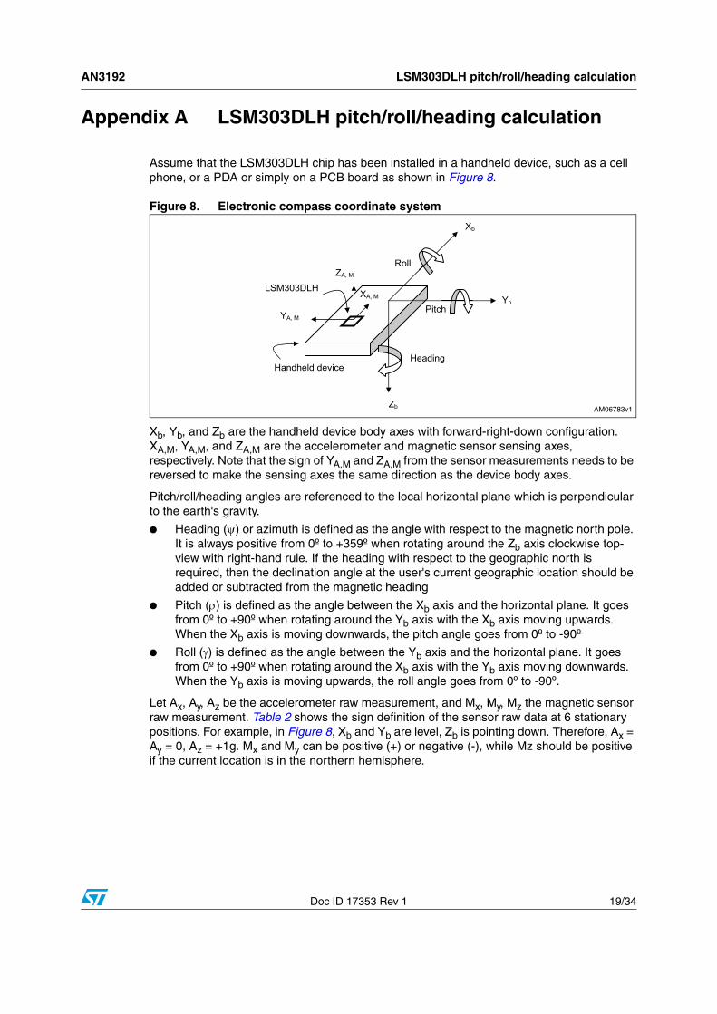
Assume that the LSM303DLH chip has been installed in a handheld device, such as a cell phone, or a PDA or simply on a PCB board as shown in Figure 8.

Figure 8. Electronic compass coordinate system

Xb, Yb, and Zb are the handheld device body axes with forward-right-down configuration. XA,M, YA,M, and ZA,M are the accelerometer and magnetic sensor sensing axes, respectively. Note that the sign of YA,M and ZA,M from the sensor measurements needs to be reversed to make the sensing axes the same direction as the device body axes.

Pitch/roll/heading angles are referenced to the local horizontal plane which is perpendicular to the earth's gravity.

● Heading (ψ) or azimuth is defined as the angle with respect to the magnetic north pole. It is always positive from 0º to +359º when rotating around the Zb axis clockwise top-view with right-hand rule. If the heading with respect to the geographic north is required, then the declination angle at the user's current geographic location should be added or subtracted from the magnetic heading

● Pitch (ρ) is defined as the angle between the Xb axis and the horizontal plane. It goes from 0º to +90º when rotating around the Yb axis with the Xb axis moving upwards. When the Xb axis is moving downwards, the pitch angle goes from 0º to -90º

● Roll (γ) is defined as the angle between the Yb axis and the horizontal plane. It goes from 0º to +90º when rotating around the Xb axis with the Yb axis moving downwards. When the Yb axis is moving upwards, the roll angle goes from 0º to -90º.

Let Ax, Ay, Az be the accelerometer raw measurement, and Mx, My, Mz the magnetic sensor raw measurement. Table 2 shows the sign definition of the sensor raw data at 6 stationary positions. For example, in Figure 8, Xb and Yb are level, Zb is pointing down. Therefore, Ax = Ay = 0, Az = +1g. Mx and My can be positive (+) or negative (-), while Mz should be positive if the current location is in the northern hemisphere.

LSM303DLH pitch/roll/heading calculation AN3192

20/34 Doc ID 17353 Rev 1

A.1 Pitch/roll calculationWhen the device is at an arbitrary 3D position X'b, Y'b, and Z'b, there are a few rotation procedures to rotate the device from the local level frame Xb, Yb, and Zb, shown in Figure 8, to that 3D position. Different rotation procedures result in different rotation matrix. The aircraft convention of angle rotation is used in this application note.

Firstly, rotate the handheld device around the Zb axis clockwise at an angle (ψ) with the view from the origin to downwards. Then rotate the device around Yb at an angle (ρ) with Xb moving upwards. Then rotate the device around Xb at an angle (γ) with Yb moving downwards. The new device body axes become X'b, Y'b, and Z'b, as shown in Figure 9.

Figure 9. Rotation procedures

Then each rotation matrix is:

Equation 5

Table 2. Sign definition of LSM303DLH sensor raw measurements

Stationary position

Accelerometer (signed integer) Magnetic sensor (signed integer)

Ax Ay Az Mx My Mz

Zb down 0 0 +1g + or - + or - +

Zb up 0 0 -1g + or - + or - -

Yb down 0 +1g 0 + or - + + or -

Yb up 0 -1g 0 + or - - + or -

Xb down +1g 0 0 + + or - + or -

Xb up -1g 0 0 - + or - + or -

⎥⎥⎥

⎦

⎤

⎢⎢⎢

⎣

⎡ψψ−ψψ

=ψ

100

0cossin

0sincos

R

AN3192 LSM303DLH pitch/roll/heading calculation

Doc ID 17353 Rev 1 21/34

Equation 6

Equation 7

And the relationship between X'b/Y'b/Z'b and Xb/Yb/Zb is:

Equation 8

In the local horizontal plane, as shown in Figure 8, Xb = Yb = 0, Zb = +1g. At X'b/Y'b/Z'b, the LSM303DLH accelerometer raw measurements are Ax, Ay, and Az which are signed integer in terms of LSBs. Let Ax1, Ay1, and Az1 be the normalized values after applying accelerometer calibration parameters into Ax, Ay, and Az. So Ax1, Ay1, and Az1 become floating point values less than 1 in terms of g (earth gravity), and the root sum of their squared values should be equal to 1 when the accelerometer is still. Then Equation 8 becomes:

Equation 9

Therefore, pitch and roll angle can be calculated as:

Equation 10

Note: When pitch = ±90º, roll should be set to 0º to avoid singularity

The arcsin function has good linearity between about -45º to +45º, so the accuracy of the pitch and roll calculation degrades when tilt angles exceed this range

Normalized accelerometer measurement Az1 is not used for the pitch and roll calculation. But it can be used to check if the magnitude is equal to 1. If not, then it

means linear acceleration or angular acceleration is detected.

⎥⎥⎥

⎦

⎤

⎢⎢⎢

⎣

⎡

ρρ

ρ−ρ=ρ

cos0sin

010

sin0cos

R

⎥⎥⎥

⎦

⎤

⎢⎢⎢

⎣

⎡

γγ−γγ=γ

cossin0

sincos0

001

R

⎥⎥⎥

⎦

⎤

⎢⎢⎢

⎣

⎡⋅

⎥⎥⎥

⎦

⎤

⎢⎢⎢

⎣

⎡

γρψγρ+ψγ−ψγ+γρψγρψγρ+ψγψγ−γρψ

ρ−ψρψρ=

⎥⎥⎥

⎦

⎤

⎢⎢⎢

⎣

⎡=

⎥⎥⎥

⎦

⎤

⎢⎢⎢

⎣

⎡

ψργ

b

b

b

b

b

b

b

b

b

Z

Y

X

coscossincossincossinsinsincossincos

sincossinsinsincoscossincossinsincos

sinsincoscoscos

Z

Y

X

RRR

'Z

'Y

'X

⎥⎥⎥

⎦

⎤

⎢⎢⎢

⎣

⎡⋅

⎥⎥⎥

⎦

⎤

⎢⎢⎢

⎣

⎡

γρψγρ+ψγ−ψγ+γρψγρψγρ+ψγψγ−γρψ

ρ−ψρψρ=

⎥⎥⎥

⎦

⎤

⎢⎢⎢

⎣

⎡

1

0

0

coscossincossincossinsinsincossincos

sincossinsinsincoscossincossinsincos

sinsincoscoscos

A

A

A

1z

1y

1x

( ))cos/Aarcsin(Roll

AarcsinPitch

1y

1x

ρ=γ=−=ρ=

21z

21y

21x AAAA ++=

LSM303DLH pitch/roll/heading calculation AN3192

22/34 Doc ID 17353 Rev 1

A.2 Heading calculationFor the heading calculation, 3-axis magnetic sensor measurements need to be normalized by applying magnetic sensor calibration parameters and then reflected onto the horizontal plane by tilt compensation, as shown in Figure 10.

Figure 10. Heading calculation

If the device rotates from Xb/Yb/Zb to X''b/Y''b/Z''b by roll angle rotation followed by pitch angle rotation, then

Equation 11

Let Mx1, My1, and Mz1 be the normalized magnetic sensor measurements after applying calibration parameters correction into magnetic sensor raw measurements Mx, My, and Mz at new positions X''b/Y''b/Z''b. Mx, My and Mz which are signed integer in terms of LSBs, while Mx1, My1, and Mz1 are floating point values less than 1 in terms of the magnetic field strength, and the square root of the sum squared values should be equal to 1 when the there is no external interference magnetic field. Then from Equation 11, tilt compensated magnetic sensor measurements Mx2, My2, and Mz2 can be obtained as:

Equation 12

⎥⎥⎥

⎦

⎤

⎢⎢⎢

⎣

⎡⋅

⎥⎥⎥

⎦

⎤

⎢⎢⎢

⎣

⎡

ργγργ−ργ−γργ

ρρ=

⎥⎥⎥

⎦

⎤

⎢⎢⎢

⎣

⎡=

⎥⎥⎥

⎦

⎤

⎢⎢⎢

⎣

⎡−ρ

−γ

b

b

b

b

b

b11

b

b

b

''Z

''Y

''X

coscossinsincos

cossincossinsin

sin0cos

''Z

''Y

''X

RR

Z

Y

X

ργ+γ+ργ−=

ργ−γ+ργ=

ρ+ρ=

coscosMsinMsincosMM

cossinMcosMsinsinMM

sinMcosMM

1z1y1x2z

1z1y1x2y

1z1x2x

AN3192 LSM303DLH pitch/roll/heading calculation

Doc ID 17353 Rev 1 23/34

Therefore,

Equation 13

The magnitude should also be equal to 1. If not, it means that the

external magnetic interference field is detected or a pitch/roll error is present.

Because the accelerometer measurements cannot distinguish earth’s gravity from linear acceleration or angular acceleration, fast motion causes pitch/roll calculation error which then directly introduces an error to the heading calculation. In most cases, the fast motion doesn't last long and the device goes back to a stationary position. So the heading accuracy in an electronic compass means static accuracy when the device is still or without acceleration.

0 M and 0 M for 270

0 M and 0 M for 90

0 M and 0 M for MM

arctan360

0 M for MM

arctan180

0 M and 0 M for MM

arctanHeading

y2x2

y2x2

y2x22x

2y

x22x

2y

y2x22x

2y

>=°=

<=°=

<=>⎟⎠

⎞⎜⎝

⎛+°=

<⎟⎠

⎞⎜⎝

⎛+°=

>=>⎟⎠

⎞⎜⎝

⎛=ψ=

22z

22y

22x MMMM ++=

Accelerometer calibration method AN3192

24/34 Doc ID 17353 Rev 1

Appendix B Accelerometer calibration method

Let's consider accelerometer calibration at 6 stationary positions, as shown in Table 2. Equation 3 can be rewritten as:

Equation 14

Or

Equation 15

Where,

Matrix X is the 12 calibration parameters that need to be determined

Matrix w is sensor raw data LSBs collected at 6 stationary positions

Matrix Y is the known normalized earth gravity vector

For example,

● At Zb down position (P1 position), and assume that at Zb down

position, n1 sets of accelerometer raw data Ax, Ay, and Az have been collected. Then,

Equation 16

Where,

The matrix Y1 has the same row of [ 0 0 1 ]

The matrix W1 contains raw data in the format of LSBs

● At Zb up position (P2 position), and assume that at Zb up position, n2 sets of accelerometer raw data Ax, Ay, and Az have been collected. Then,

Equation 17

● At Yb down position (P3 position), and assume that at Yb down

position, n3 sets of accelerometer raw data Ax, Ay, and Az have been collected. Then,

Equation 18

[ ] [ ]⎥⎥⎥⎥

⎦

⎤

⎢⎢⎢⎢

⎣

⎡

⋅=

302010

332313

322212

312111

zyx1z1y1x

ACCACCACC

ACCACCACC

ACCACCACC

ACCACCACC

1AAAAAA

XwY ⋅=

[ ] [ ]100AAA 1z1y1x =

[ ][ ]

4x1n1zP1yP1xP1

3x1n1

1AAAw

100Y

=

=

[ ] [ ]100AAA 1z1y1x −=

[ ][ ]

4x2n2zP2yP2xP2

3x2n2

1AAAw

100Y

=

−=

[ ] [ ]010AAA 1z1y1x =

[ ][ ]

4x3n3zP3yP3xP3

3x3n3

1AAAw

010Y

=

=

AN3192 Accelerometer calibration method

Doc ID 17353 Rev 1 25/34

● At Yb up position (P4 position), and assume that at Yb up

position, n4 sets of accelerometer raw data Ax, Ay, and Az have been collected. Then,

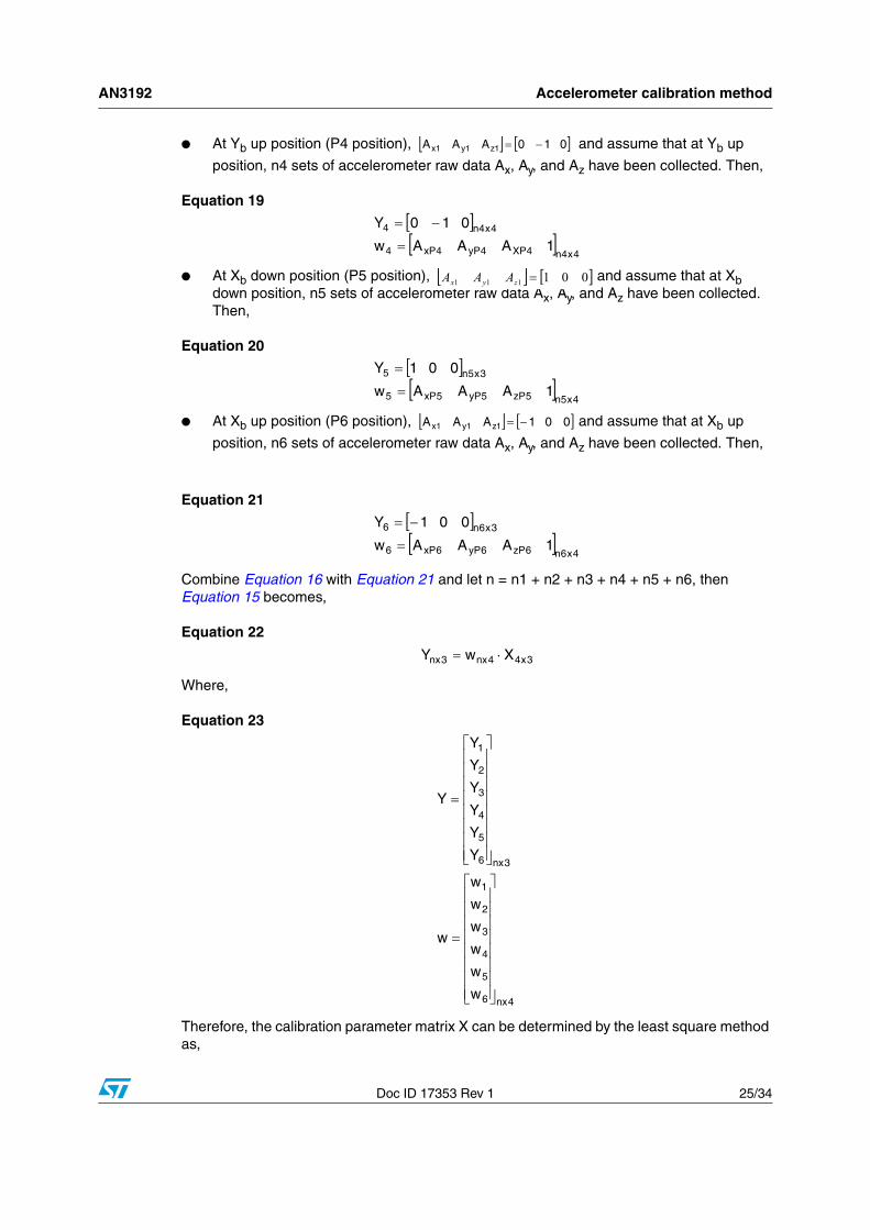
Equation 19

● At Xb down position (P5 position), and assume that at Xb down position, n5 sets of accelerometer raw data Ax, Ay, and Az have been collected. Then,

Equation 20

● At Xb up position (P6 position), and assume that at Xb up

position, n6 sets of accelerometer raw data Ax, Ay, and Az have been collected. Then,

Equation 21

Combine Equation 16 with Equation 21 and let n = n1 + n2 + n3 + n4 + n5 + n6, then Equation 15 becomes,

Equation 22

Where,

Equation 23

Therefore, the calibration parameter matrix X can be determined by the least square method as,

[ ] [ ]010AAA 1z1y1x −=

[ ][ ]

4x4n4XP4yP4xP4

4x4n4

1AAAw

010Y

=

−=

[ ] [ ]001111 =zyx AAA

[ ][ ]

4x5n5zP5yP5xP5

3x5n5

1AAAw

001Y

=

=

[ ] [ ]001AAA 1z1y1x −=

[ ][ ]

4x6n6zP6yP6xP6

3x6n6

1AAAw

001Y

=

−=

3x44nx3nx XwY ⋅=

4nx6

5

4

3

2

1

3nx6

5

4

3

2

1

w

w

w

w

w

w

w

Y

Y

Y

Y

Y

Y

Y

⎥⎥⎥⎥⎥⎥⎥⎥

⎦

⎤

⎢⎢⎢⎢⎢⎢⎢⎢

⎣

⎡

=

⎥⎥⎥⎥⎥⎥⎥⎥

⎦

⎤

⎢⎢⎢⎢⎢⎢⎢⎢

⎣

⎡

=

Accelerometer calibration method AN3192

26/34 Doc ID 17353 Rev 1

Equation 24

Where,

[ ] YwwwX T1T ⋅⋅⋅=−

Tw

[ ] 1T ww−

⋅

means matrix transpose

means matrix inverse

AN3192 Magnetic sensor calibration method

Doc ID 17353 Rev 1 27/34

Appendix C Magnetic sensor calibration method

C.1 Step 1: Soft-iron effect verificationIt is always good to know if the device has soft-iron interference before choosing which model for the identification of the calibration parameters, tilted ellipsoid, or non-tilted ellipsoid. This can be done by performing 3D rotations in a clean environmental area. Then plot the collected magnetic sensor raw data to check if there is a soft-iron interference field inside the device. This set of data is not used for the following magnetic sensor calibration. However, in practical situations, three 2D full round rotations may not be easy to perform. Then an amount of 3D rotations data can be used for rough field calibration.

An example plot of 3D rotations data and three 2D full round rotations data is shown in Figure 11. It is obvious that this electronic compass has a built-in soft-iron effect.

Figure 11. 3D rotations plus three 2D full round rotations

C.2 Step 2: Hard-iron, soft-iron and scale factor compensationIf there is soft-iron distortion, the 3D rotations show a tilt ellipsoid which can be described as the following equation:

Equation 25

where:

● x0, y0, z0 are the offsets M_OSi (i = x, y, z) caused by hard-iron distortion

● x, y, z are magnetic sensor raw data Mx, My and Mz

● a, b, c are the semi-axes lengths,

● d, e, f are cross axis effect to make the ellipsoid tilted,

● R is a constant of the earth’s magnetic field strength.

( ) ( ) ( ) ( )( ) ( )( ) ( )( ) 22222

2

2

2

2

2

Rf

0zz0yy

e

0zz0xx

d

0yy0xx

c

0zz

b

0yy

a

0xx=

−−+

−−+

−−+

−+

−+

−

Magnetic sensor calibration method AN3192

28/34 Doc ID 17353 Rev 1

If there is no soft-iron distortion inside the device, or the soft-iron effect is very small and can be ignored, then the ellipsoid from 3D rotations is not tilted. So the soft-iron matrix [M_si] is a 3x3 identity matrix and Equation 25 can be simplified as:

Equation 26

Therefore, the least square fitting ellipsoid method can be used to discover the parameters of M_SCi, M_OSi (i = x, y, z) and [M_si]. The magnetic sensor raw data used here could be three 2D full round rotations, or 3D rotations, or both.

Applying these parameters to the collected 3D rotations data and three 2D full round rotations, the plot is shown in Figure 12. Now the shifted tilted ellipsoid becomes a centered unit sphere.

Figure 12. After hard-iron, soft-iron, and scale factor compensation

Let's assume there is no soft-iron distortion. The soft-iron matrix [M_si] is a 3x3 identity matrix. Then Equation 26 can be rewritten as:

Equation 27

After three 2D full round rotations magnetic sensor raw data have been collected, it is possible to combine Mx, My, and Mz as column vector and row vector. Then Equation 27 becomes,

( ) ( ) ( ) 22

2

2

2

2

2

Rc

0zz

b

0yy

a

0xx=

−+

−+

−

[ ]

⎥⎥⎥⎥⎥⎥⎥⎥⎥⎥⎥⎥⎥⎥

⎦

⎤

⎢⎢⎢⎢⎢⎢⎢⎢⎢⎢⎢⎢⎢⎢

⎣

⎡

−−−

⋅−−=

202

2202

220

22

2

2

2

2

02

2

02

20

222

zc

ay

b

axRa

c

ab

a

z2c

a

y2b

ax2

1zyzyxx

AN3192 Magnetic sensor calibration method

Doc ID 17353 Rev 1 29/34

Equation 28

The least square method can be applied to determine the parameters X vector as:

Equation 29

Then,

Equation 30

And,

Equation 31

Let,

Equation 32

Then Equation 26 becomes,

Equation 33

Therefore,

Equation 34

[ ] 1x66nx1nx XHw ⋅=

[ ] wHHHX T1T ⋅=−

))5(X2/()3(XzOS_M

))4(X2/()2(XyOS_M

2/)1(XxOS_M

0z

0y

0x

⋅==

⋅==

==

)5(X/AC

)4(X/AB

z)5(Xy)4(Xx)6(XRaA 20

20

20

22

==

⋅+⋅++==

zz

yy

xx

OS_MMzz

OS_MMyy

OS_MMxx

−=

−=

−=

1C

zzB

yyA

xx 222

=++

CSC_M

BSC_M

ASC_M

z

y

x

=

=

=

Magnetic sensor calibration method AN3192

30/34 Doc ID 17353 Rev 1

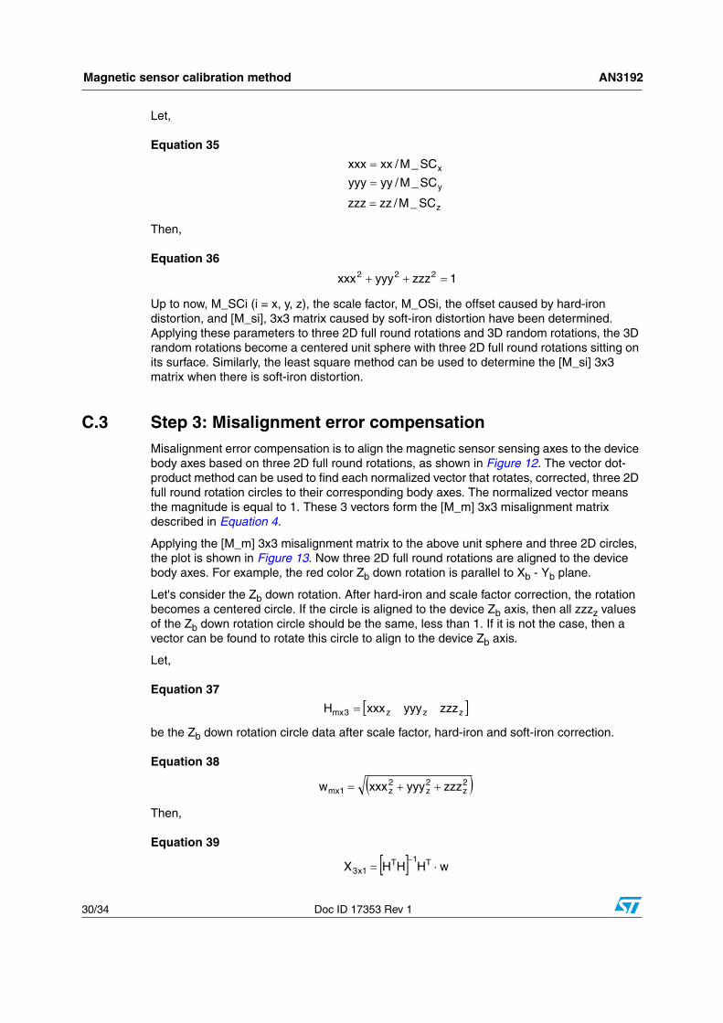
Let,

Equation 35

Then,

Equation 36

Up to now, M_SCi (i = x, y, z), the scale factor, M_OSi, the offset caused by hard-iron distortion, and [M_si], 3x3 matrix caused by soft-iron distortion have been determined. Applying these parameters to three 2D full round rotations and 3D random rotations, the 3D random rotations become a centered unit sphere with three 2D full round rotations sitting on its surface. Similarly, the least square method can be used to determine the [M_si] 3x3 matrix when there is soft-iron distortion.

C.3 Step 3: Misalignment error compensationMisalignment error compensation is to align the magnetic sensor sensing axes to the device body axes based on three 2D full round rotations, as shown in Figure 12. The vector dot-product method can be used to find each normalized vector that rotates, corrected, three 2D full round rotation circles to their corresponding body axes. The normalized vector means the magnitude is equal to 1. These 3 vectors form the [M_m] 3x3 misalignment matrix described in Equation 4.

Applying the [M_m] 3x3 misalignment matrix to the above unit sphere and three 2D circles, the plot is shown in Figure 13. Now three 2D full round rotations are aligned to the device body axes. For example, the red color Zb down rotation is parallel to Xb - Yb plane.

Let's consider the Zb down rotation. After hard-iron and scale factor correction, the rotation becomes a centered circle. If the circle is aligned to the device Zb axis, then all zzzz values of the Zb down rotation circle should be the same, less than 1. If it is not the case, then a vector can be found to rotate this circle to align to the device Zb axis.

Let,

Equation 37

be the Zb down rotation circle data after scale factor, hard-iron and soft-iron correction.

Equation 38

Then,

Equation 39

z

y

x

SC_M/zzzzz

SC_M/yyyyy

SC_M/xxxxx

=

==

1zzzyyyxxx 222 =++

[ ]zzz3mx zzzyyyxxxH =

( )2z

2z

2z1mx zzzyyyxxxw ++=

[ ] wHHHX T1T1x3 ⋅=

−

AN3192 Magnetic sensor calibration method

Doc ID 17353 Rev 1 31/34

So the normalized rotation vector for Zb down rotation is,

Equation 40

Similarly, the normalized rotation vectors Rx and Ry for Xb down rotation and Yb down rotation can be found. Then the final misalignment compensation matrix is,

Equation 41

Figure 13. After misalignment compensation

( )222z )3(X)2(X)1(X/XR ++=

[ ]zyx3x3 RRRm_M =

References AN3192

32/34 Doc ID 17353 Rev 1

6 References

1. STMicroelectronics, Inc. LSM303DLH sensor module datasheet

http://www.st.com/stonline/products/families/sensors/motion_sensors/lsm303dlh.htm

2. Honeywell, Inc. Applications of Magnetoresistive Sensors in Navigation Systems

http://www.ssec.honeywell.com/position-sensors/datasheets/sae.pdf

3. Honeywell, Inc. Applications of Magnetic Sensors for Low Cost Compass Systems

http://www.ssec.honeywell.com/magnetic/datasheets/lowcost.pdf

AN3192 Revision history

Doc ID 17353 Rev 1 33/34

7 Revision history

Table 3. Document revision history

Date Revision Changes

02-Aug-2010 1 Initial release.

AN3192

34/34 Doc ID 17353 Rev 1

Please Read Carefully:

Information in this document is provided solely in connection with ST products. STMicroelectronics NV and its subsidiaries (“ST”) reserve theright to make changes, corrections, modifications or improvements, to this document, and the products and services described herein at anytime, without notice.

All ST products are sold pursuant to ST’s terms and conditions of sale.

Purchasers are solely responsible for the choice, selection and use of the ST products and services described herein, and ST assumes noliability whatsoever relating to the choice, selection or use of the ST products and services described herein.

No license, express or implied, by estoppel or otherwise, to any intellectual property rights is granted under this document. If any part of thisdocument refers to any third party products or services it shall not be deemed a license grant by ST for the use of such third party productsor services, or any intellectual property contained therein or considered as a warranty covering the use in any manner whatsoever of suchthird party products or services or any intellectual property contained therein.

UNLESS OTHERWISE SET FORTH IN ST’S TERMS AND CONDITIONS OF SALE ST DISCLAIMS ANY EXPRESS OR IMPLIEDWARRANTY WITH RESPECT TO THE USE AND/OR SALE OF ST PRODUCTS INCLUDING WITHOUT LIMITATION IMPLIEDWARRANTIES OF MERCHANTABILITY, FITNESS FOR A PARTICULAR PURPOSE (AND THEIR EQUIVALENTS UNDER THE LAWSOF ANY JURISDICTION), OR INFRINGEMENT OF ANY PATENT, COPYRIGHT OR OTHER INTELLECTUAL PROPERTY RIGHT.

UNLESS EXPRESSLY APPROVED IN WRITING BY AN AUTHORIZED ST REPRESENTATIVE, ST PRODUCTS ARE NOTRECOMMENDED, AUTHORIZED OR WARRANTED FOR USE IN MILITARY, AIR CRAFT, SPACE, LIFE SAVING, OR LIFE SUSTAININGAPPLICATIONS, NOR IN PRODUCTS OR SYSTEMS WHERE FAILURE OR MALFUNCTION MAY RESULT IN PERSONAL INJURY,DEATH, OR SEVERE PROPERTY OR ENVIRONMENTAL DAMAGE. ST PRODUCTS WHICH ARE NOT SPECIFIED AS "AUTOMOTIVEGRADE" MAY ONLY BE USED IN AUTOMOTIVE APPLICATIONS AT USER’S OWN RISK.

Resale of ST products with provisions different from the statements and/or technical features set forth in this document shall immediately voidany warranty granted by ST for the ST product or service described herein and shall not create or extend in any manner whatsoever, anyliability of ST.

ST and the ST logo are trademarks or registered trademarks of ST in various countries.

Information in this document supersedes and replaces all information previously supplied.

The ST logo is a registered trademark of STMicroelectronics. All other names are the property of their respective owners.

© 2010 STMicroelectronics - All rights reserved

STMicroelectronics group of companies

Australia - Belgium - Brazil - Canada - China - Czech Republic - Finland - France - Germany - Hong Kong - India - Israel - Italy - Japan - Malaysia - Malta - Morocco - Philippines - Singapore - Spain - Sweden - Switzerland - United Kingdom - United States of America

www.st.com