ANÁLISE ECONÓMICA •••• 16

Manuel González Gómez, Philippe Polomé y Albino Prada Blanco Departamento de Economía Aplicada

Universidade de Vigo Lagoas-Marcosende s/n. 36200 Vigo.

Mgzlez@uvigo.es

FUNCIONAL FORMS, SAMPLING CONSIDERATIONS AND ESTIMATION OF DEMAND FOR PROTECTED NATURAL AREAS:

THE CÍES ISLANDS CASE STUDY IN GALICIA (SPAIN).

CONSELLO EDITOR: Xoaquín Alvarez Corbacho, Economía Aplicada. UC; Manuel Antelo Suárez, Fundamentos da Análise Económica. USC; Juan J. Ares Fenández, Fundamentos da Análise Económica. USC; Xesús Leopoldo Balboa López, Historia Contemporánea. USC; Xosé Manuel Beiras Torrado, Economía Aplicada. USC; Joam Carmona Badía, Historia e Institucións Económicas. USC; Luis Castañón Llamas Economía Aplicada. USC; Xoaquín Fernández Leiceaga, Economía Aplicada. USC; Lourenzo Fernández Prieto, Historia Contemporánea. USC; Ignacio García Jurado, Estatística e Investigación Operativa. USC; Mª do Carmo García Negro, Economía Aplicada. USC; Xesús Giraldez Rivero, Historia e Institucións Económicas. USC. Wenceslao González Manteiga, Estatística e Investigación Operativa. USC; Manuel Jordán Rodríguez, Economía Aplicada. USC; Rubén C. Lois González, Xeografía. USC; Edelmiro López Iglesias, Economía Aplicada. USC; José A. López Taboada, Historia e Institucións Económicas. USC. Alberto Meixide Vecino, Fundamentos da Análise Económica. USC; Emilio Pérez Touriño, Economía Aplicada. USC; Miguel Pousa Hernández Economía Aplicada. USC; Albino Prada Blanco, Economía Aplicada. UV;

Carlos Ricoy Riego, Fundamentos da Análise Económica. USC; José Mª da Rocha Alvarez, Fundamentos da Análise Económica. UV; Xavier Rojo Sánchez, Economía Aplicada. USC; José Santos Solla, Xeografía. USC; Juan Surís Regueiro, Economía Aplicada. UV; Manuel Varela Lafuente, Economía Aplicada. UV; COORDENADORES DA EDICIÓN: - Área de Análise Económica Juan J. Ares Fernández - Área de Economía Aplicada Manuel Jordán Rodríguez - Área de Historia Lourenzo Fernández Prieto - Área de Xeografía Rubén C. Lois González, ENTIDADES COLABORADORES Fundación Caixa Galicia Consello Económico e Social de Galicia Fundación Feiraco Instituto de Estudios Económicos de Galicia Pedro Barrié de la Maza

Edita: Servicio de Publicacións da Universidade de Santiago de Compostela ISSN: 1138 - 0713 D.L.G.: C-1689-97

1

Abstract

In this paper, we present estimates of several models of demand for a natural area using data from surveys on visitors and non-visitors. The estimates take into ac-count the problems of: demand specification, measurement of the cost and of the de-mand, choosing sampling scheme, and handling the sample. Considering these alter-natives allows us to select a model of demand under improved conditions and frees us from initial restrictive hypothesis. The results in terms of prediction of demand and consumer surplus estimates are quite dissimilar, stressing the importance of compar-ing various models that encompass the range of possible options

Keywords: Travel Cost Method, Endogeneous Stratification, Truncation, Demand specification, Hurdle models.

Resumen

En este trabajo presentamos estimaciones de diferentes modelos de demanda para un espacio recreativo a partir de la información de entrevistas a visitantes y no visitantes. La estimación tiene en cuenta los problemas de especificación de demanda, de medición del coste y demanda, de elección de una técnica de muestreo y de trata-miento de la muestra. La consideración de estas alternativas permite elegir una mode-lización en mejores condiciones y nos aleja de supuestos iniciales restrictivos. Los resultados en términos de predicción de la demanda y estimación del excedente son bastante divergentes, resaltando la importancia de comparar diferentes modelos que incluyan el espectro de opciones potenciales.

Palabras Clave: método de los costes de viaje, estratificación endógena, truncación, especificación de demanda, modelos valla.

2

1. Introduction

Quantification of the value of the environmental services generated by nature

areas, on the basis of a measurement of public preferences, enables us to determine

the benefits generated and thus to carry out an efficiency analysis. Once this effi-

ciency value is known, projects can be evaluated ex–ante and the results of interven-

tion, ex-post; a cost-effectiveness analysis permits the least-cost invention to be se-

lected, and a cost-benefit analysis permits the social return for a project or interven-

tion to be calculated. The methods utilised for such quantification are contingency

valuation, hedonic pricing and travel costs.

There are numerous applications of the travel cost and contingency valuation

methods particularly. The travel cost method utilises costs and observed behaviour in

order to estimate the demand function and calculate a measurement of welfare. The

number of visits is considered to be a measure of the demand for an area of nature,

whereas the sum of both the travelling and opportunity costs is taken as a ‘proxy’ of

the price variable. In recent decades alternatives have been proposed for specific as-

pects of the estimation process, namely, functional forms, dependent variables, en-

dogenous stratification and in situ sampling, or the costs to be considered relevant.

It is common practice in applications to initially opt for a concrete specifica-

tion and to then proceed to the calculation of the measure of welfare (Riera et al.,

1994; Garrido et al., 1996; González, 1997, Pérez y Barreiro, 1998, Farré, 1998; Del

Saz y Pérez, 1999 for Spain). There are also studies that compare the effect of differ-

ent specifications; Hanley (1989) obtains results with a squared functional form and

with cost and demand logarithms; Willis and Garrod (1991) estimate a demand func-

tion with truncation utilising several functional forms; Hellerstein (1991) utilises a

semi-logarithmic functional form and two discrete distributions – the Poisson and

negative binomial distributions; Dobbs (1993) employs discrete and continuous mod-

els and also analyses the effect of different sample size; Englin and Lambert (1995)

compare results using two discrete distributions – again the Poisson and negative bi-

nomial distributions; and finally, Englin and Shonkwiler (1995) compare the conse-

quences of different handling of a sample taken in the area of the visit (in situ sam-

pling).

3

In this paper, we systemise and amplify these comparisons. Five kinds of

problems that are encountered when estimating demand for an area of nature are con-

sidered with a view to calculating a measure of welfare. The first of these problems is

the choice of sampling method. In order to collect information, a sample is frequently

obtained in the area itself, but it is also possible to utilise a simple random sample

taken within the catchment area of the nature park in question. The advantages of both

of these methods will be compared below. The second problem refers to the handling

of samples taken in the visited area. These are not simple random samples, for which

reason the conventional estimation techniques are not valid. We will, therefore, dis-

cuss three ways of modelling these samples. The third problem we tackle is the very

definition of demand for an area of nature. Usually this is measured on the basis of the

number of visits during a specific period of time. However, intuitively it can be af-

firmed that the stay in the nature area also forms part of the demand. We will there-

fore contrast results utilising conventional measures, and also a measure that will in-

corporate the period of stay in the nature area. The fourth problem deals with a speci-

fication of the demand. Either a discrete distribution – where demand is expressed in

levels - or a continuous distribution - where demand can be expressed in levels or

logarithms - can be employed. Hence, two discrete distributions (Poisson and negative

binomial) and one continuous distribution (normal) will be compared. Finally, the

fifth problem is measurement of price on the basis of displacement cost. Seven defi-

nitions of cost are considered, depending on which expenses are considered appropri-

ate for inclusion in the displacement cost. To sum up, this procedure incorporating a

wide range of options is naturally complex in calculation terms, but it does permit a

determination of the welfare measure on the basis of more complete information and

without having to jettison options from the outset.

To complement estimations of the benefits generated by an area of nature, it is

common practice to study the demand for an area by considering that substitutes exist

(discrete choice models or random utility models). Such a focus permits an analysis of

changes to welfare resulting from modifications to the nature areas in terms of quality

or quantity. In our particular case, the Cíes Islands (off the coast of Vigo, Spain) rep-

resent the only island enclave in an estuary of the Iberian Peninsula that is designated

a natural park. In addition the islands can count on infrastructures for recreational use

and on conservation measures (absence of motor vehicles, urbanisation and waste,

4

and special reclamation and conservation programmes for flora and fauna). These

factors permit the affirmation that near substitutes do not in fact exist. A multitude of

secondary options distributed throughout the entire peninsula do exist, but to include

them all in a demand system and to collect the necessary data would be an intermina-

ble and enormously difficult process.

Our next section (Section 2) will describe the problems of demand specifica-

tion (functional forms), sample handling, and demand measurement. In Section 3 we

will tackle the application to the Cíes Islands of the in situ sampling technique and

describe the different measurements of displacement cost. In Section 4 we will de-

scribe the application to the Cíes Islands of a case of simple random sampling of visi-

tors and non-visitors representative of the province of Pontevedra (the immediate

catchment area for the Islands). Finally, Section 5 will describe our conclusions.

2. Functional forms, sample handling and demand measurement

2. a. Functional forms

Some authors estimate demand for a recreation area by taking the endogenous

variable as continuous and assuming it is an option for dealing with the number of

journeys that individuals make (Willis and Garrod, 1991; Smith and Desvouges,

1988; and Dobbs, 1993, among others). Another option, predominant in recent appli-

cations, explicitly takes into account the discrete nature of the dependent variable. In

this case the negative binomial (usually in the form BN2, see Cameron and Trivedi,

1998) and Poisson (Hellerstein and Mendelsohn, 1993) probability functions are those

most utilised. The BN2 is essentially a Poisson model in which the non-observed het-

erogeneity between different individuals is modelled by means of a gamma distrib-

uted noise. In this way one of the Poisson model restrictions is avoided, namely, the

property of equi-dispersion - which is to say, the mean of the distribution should be

equal to its variance. Very often this property is not verified in practice, and the BN2

distribution is therefore more appropriate than the Poisson. In theory it would be pos-

sible also to employ other distributions, but the Poisson and the BN2 are the only dis-

tributions for which the necessary results have been developed for all the ways of

handling samples that are under consideration here. It must be emphasised that if cost

5

expressed in logarithms is taken for the two discrete models, an infinite consumer

surplus would almost invariably be imposed (Appendix I). For this reason, only cost

expressed in levels for the discrete models has been taken into consideration.

Four possibilities exist for modelling the endogenous variable as continuous.

These are: the LinLin model, in which - assuming a normal distribution - both the en-

dogenous variable and the cost are expressed in levels; the LinLog model, with the

endogenous variable distributed normally in levels and with cost expressed in loga-

rithms; the LogLin model, with the logarithm of the endogenenous variable distrib-

uted normally and with cost expressed in levels; and finally the LogLog model, with

the logarithm of the endogenous variable distributed normally and with cost expressed

in logarithms. For the LogLin and LogLog models, it is not possible to predict null

values for the endogenous variable (the zero logarithm is not defined), and hence, the

consumer surplus will always be infinite. To avoid this problem, 1 is added to the en-

dogenous variable before making the estimation. Distributions other than the normal

distribution could also be considered but results do not exist for all the sample treat-

ments under consideration.

To sum up then, there are six basic models, one for each definition of the en-

dogenous variable. These are summarised in Table 1, where Y is the endogenous vari-

able, p is the displacement cost with coefficient , is a constant that represents the

linear combination of all the other regressors multiplied by their respective coeffi-

cients, E is the expectation operator, and finally y exp is the exponential operator.

Table 1: Basic models

Poisson, BN2: EY = exp( + p )

LinLin: Y = + p + u u n(0, ²) EY = + p

LinLog Y = + ln(p) + u u n(0, ²) EY = + ln(p)

LogLin ln(Y+1) = + p + u u n(0, ²) EY = exp( + p + ²/2) - 1

LogLog ln(Y+1) = + ln(p) + u u n(0, ²) EY = p exp( + ²/2) - 1

6

2. b. Sample handling

There are basically two ways of obtaining a sample via observations of quanti-

ties of recreational demand. The first, and probably the most common way, is to

sample within the recreational area. The second obtains a simple random sample from

a reference population. The majority of applications make use of the former (Pérez y

Barreiro, 1998, Farré, 1998; González, 1997, Garrido, 1996, Riera et al., 1994; Cam-

pos et al, 1996). The principal reason for obtaining an in situ sample is that of compil-

ing information on costs, especially in cases where the visitors may be from very di-

verse origins. Nevertheless, this is not simple random sampling, and therefore the

conventional techniques for calculation of demand should be modified (Shaw, 1988).

In particular, given that there is no null demand with this kind of sampling, the ob-

served demand is truncated at zero. In this paper we compare the properties of the two

sampling methods in respect of their capacity for obtaining a reliable estimate of the

consumer surplus. Section 3 presents the results obtained on the basis of a sample

taken in situ and Section 4 complements this sample with a non-visitor sample in or-

der to obtain new results.

For the sample taken in situ, we apply three handling methods: the non-

truncated method, in which there is no modification to the distribution of the endoge-

nous variable, except for the continuous models where distribution at zero is cen-

sored1 (demand can never be negative); the truncated method in which the distribution

of the endogenous variable is truncated2 at one (a sample of visitors does not include

values that are lower than one); and finally, the in situ treatment, in which the distri-

bution of the endogenous variable is modified in accordance with this kind of sample

in the way described above (see Shaw, 1988, for the continuous and Poisson models;

Englin and Shonkwiler, 1995, for the BN2 model). All the models are estimated for

maximum verisimilitude. Depending on the handling of the sample, the expectation

for the endogenous variable is modified (Table 1). (See Greene, 1999, for the cen-

sored and truncated continuous models; Cameron and Trivedi, 1998, for the truncated

and in situ discrete models; and Shaw, 1988, for the in situ continuous models).

1 See Greene (1998) for a theoretical description of these models. 2 See Greene (1998) for the continuous models and Cameron & Trivedi (1998) for the discrete models.

7

The truncated samples

A sample such as that of visitors to the Cíes Islands is truncated because no

null demand is observed. It seems therefore a good idea to build into the estimation

process the information that if no zero is found, it is not because the function to be

estimated cannot predict null values, but rather due to the configuration of the sample.

Demand theory defines consumer surplus as the area below the demand curve,

from the price that this consumer pays to the cut-off price (possibly infinite). Hence,

in order to calculate the consumer surplus it is necessary to predict the behaviour of

demand as it approaches zero. With a truncated sample this information is to be

found outside the sample space. It is thus a matter of defining demand over the entire

range of price (or cost, or any other variable) on the basis of the information obtained

from the truncated sample.

Let Yi be the displacement demand for visitor i. Based on a demand distribu-

tion (e.g. Poisson), we can define the truncated distribution, the parameters of which

are estimated from the sample. The conditional expected demand to visit E(Yi | Yi

1) can be calculated on the basis of this estimation. By construction, this conditional

demand can never be null, and hence, if we try to calculate a consumer surplus on the

basis of this conditional demand, it will of necessity be infinite. Nonetheless, it is a

well-known fact that as the displacement cost increases, the probability of a visit de-

creases. Therefore, the unconditional expected demand for a visitor is the product of

the conditional expected demand multiplied by the probability of the visit, i.e.:

E(Yi) = E(Yi | Yi 1) Pr{Yi 1}.

Now this product happens to be the expectation for the original Poisson distri-

bution. Hence, we estimate the conditional expectation from the sample utilising a

truncated distribution, and to calculate the consumer surplus we substitute the esti-

mated coefficients into the initial Poisson distribution.

The in situ samples

The in situ samples are obtained when visitors are interviewed randomly

(whether in a nature zone or in a supermarket) in the very place of the visit. By con-

8

struction, these samples are truncated given that non-visitors obviously cannot be in-

terviewed in situ. In addition, however, those who visit frequently have a greater

chance of being interviewed, and will therefore be over-represented in the resulting

sample, and inversely for those who visit the area least (Shaw, 1988). Thus, if we

calculate the average number of visits on the basis of such a sample, we will overes-

timate the real average of visits. Shaw (1988) demonstrated how a Poisson or normal

distribution, in this case, would have to be modified. Englin and Shonkwiler (1995)

extended these results to the case of a BN2 distribution. For the discrete models, the

correction consists of applying weights to the probabilities for each number of visits

in order to reflect the fact that the probability of being interviewed increases with the

number of visits. A reasoning process similar to that for the truncated samples can be

applied to the in situ samples in order to demonstrate that the unconditional expected

demand on which we calculate the surplus is the expectation of the original distribu-

tion.

2. c. Measurement of demand

The estimation of demand for an area of nature tends to use the number of vis-

its to the area as a measure of demand, based on the assumption that the duration of

these visits is constant. There are several arguments in favour of this approach; it is a

variable that is perfectly valid for a description of individual behaviour; in some cases

the nature zone does not permit stays of more than a day; there is little or no informa-

tion about average stay, and/or the study only includes visits of one day or less.

Nevertheless, we could argue that the visitor in fact does not only decide the

number of visits, but at the same time, the duration of the visits (or stay). It is gener-

ally acknowledged that length of stay in an area may play an important role in ex-

plaining demand for an area of nature - to be able to stay for several days means that

the visitor can allocate his travelling costs to a greater number of days. Bell and Lee-

worthy (1990) constructed stay in days as a function of the cost incurred by each one,

unlike the traditional versions where travelling costs are related to the number of dis-

placements made. Finally the possibility of staying more than one day in the area of

nature might well be considered an attraction rather than a cost.

9

In this paper, we utilise two measures of demand for an area of nature. The

first measure is based on the traditional notion of the number of visits, which we con-

sider here in the long term (the 5 years prior to the survey). We call this variable

‘displacement’. The second measure considers that the two variables (number of visits

and stay) are both aspects of the same demand - that of days in the park – as applied

previously by Bell and Leeworthy (1990). It would be possible to construct a system

of two simultaneous equations - one for number of visits and another for stay - but it

is considered here that both these variables can be represented in terms of the average

demand in terms of days' stay on the Islands. In order to construct this variable the

individual number of visits was multiplied by the declared number of days3 stayed by

the respondent, this number being considered a good indicator of the average individ-

ual stay. We will call this variable ‘total stay’.

Thus we can make the estimate of demand on the basis of the number of visits

or as the number of visits multiplied by length of stay. These can be then be consid-

ered as either continuous or discrete. For the continuous version, the 4 forms de-

scribed in Table 1 can be used (LinLin, LinLog, LogLin, or LogLog) under an as-

sumption of normality; in the discrete version the two usual distributions (Poisson and

BN2) can be employed. For each of these specifications, three sample treatments can

be applied (non-truncated, truncated and in situ). We thus have a total of 36 different

models.

3. Visitor sampling

The samples utilised were personal interviews with visitors to the Cíes Islands

during the summer of 1998. A complete description of these interviews can be found

in González et al (2000). Below we describe both the regressors that were employed

in order to estimate the models described in the previous section and the results of the

estimations.

Explanatory variables and definition of displacement cost

The sensitivity of the consumer surplus to the determination of the displace-

ment cost makes it necessary to refine the values utilised for this variable. The cost is

3 Part of a day is considered a day’s stay.

10

known only to the visitor and is not verifiable by others. According to Randall (1994),

the determination of the individual displacement cost on the part of the researcher is

largely arbitrary. The researcher will, therefore, only have recourse to existing prac-

tices, and any measure or estimation of welfare will depend on the chosen method.

For this application the cost variable is defined as the sum of the costs that the

visitors declare to have incurred. The costs are weighted in different ways in order to

arrive at seven definitions of the displacement cost, and the estimation process will

determine the cost that best explains the demand for each model. For the opportunity

cost of time we will consider the wage given in the working population survey4 less

the average deduction made by the tax authorities (1063 pesetas). The seven formal

definitions of cost are fully described in Appendix 2; in summarised form, these are:

Ca, total cost, a summary of all costs including nights of arrival and departure

Cn, which does not take into account nights spent away from the Islands

Cc, displacement from home to ferry port is only a cost for those who declare it so

Cd, length of stay in the Islands is irrelevant (they can be visited in a single day)

Ct, the opportunity cost of time is null (Spanish labour market inflexibility)

Cm, the cost of getting to the temporary residence is only counted for those visi-

tors whose principal motive for travelling is the visit to the Islands

Tim and C, the monetary and time costs are considered separately.

In addition to cost, variables included as possible explanatory variables are

listed as follows: the equivalent adult income according to the OECD (income), en-

quired about in terms of income bands; a green index (green), defined by the sum of

6 dichotomous variables indicating various kinds of environmentally-sensitive behav-

iour; a knowledge index for the Islands (know), defined by the sum of 6 dichotomous

variables indicating whether the respondent has visited specific areas of the Islands; a

4 Encuesta de Población Activa, a census carried out regularly by the Spanish Na-tional Employment Institute.

11

response reliability index (rel), consisting of the sum of three dichotomous variables

that cover various aspects of the degree of confidence that the interviewer feels for the

answers of the respondent; the age of the respondent (/age) normalised to the maxi-

mum band value, the sex of the respondent (sex), two dichotomous variables (djuly

and dsept) that indicate the month when the interview took place; other variables indi-

cating whether the respondent had a remunerated employment (remu), whether there

were children in the home (child), whether education was to secondary or tertiary

level (educ), whether the respondent was satisfied with the visit (satis), and finally,

whether information on the Islands had been available to the respondent before the

visit (info).

Dichotomous variables were also included that indicated which of a list of fea-

tures of the Islands the respondent considered to be the principal attractions, namely,

trekking (trkk), nature observation (nature), absence of pollution (conta), beaches

(beach) and tranquillity (tranq).

For each cost concept, the estimation of each one of the 36 models is based on

the set of 19 potential regressors described above, subsequently reduced by the elimi-

nation of variables. Firstly, chosen for each model is the cost for which the greatest

likelihood is obtained; to be called dominant cost, this is described in Table 2. Next

the elimination process utilises t-contrasts in order to identify the regressors that may

not be significant. Finally, likelihood ratio test utilised in order to check that the ini-

tial set can be reduced by more than one non-significant regressor. All the contrasts

are made at 5%. The final set of significant regressors for each model is described in

Table 2.

The proposed models are non-linear and on more than one occasion it happens

that the process of estimation does not converge with the initial set of regressors but

rather with a reduced set. Evidently the choice of this reduced set is arbitrary and the

estimations are hence less reliable. In order to make a selection for this reduced set

that minimises arbitrariness as much as possible, all the models that converged were

first estimated with the initial set of regressors. The reduced set was then defined by

the union of the final regressors (of the models that converged) with the initial set. In

Tables 2 and 4 the models that did not originally converge appear in the squares in

12

grey. Finally, some models do not converge with any set of regressors, probably indi-

cating that they do not describe the data sufficiently well.

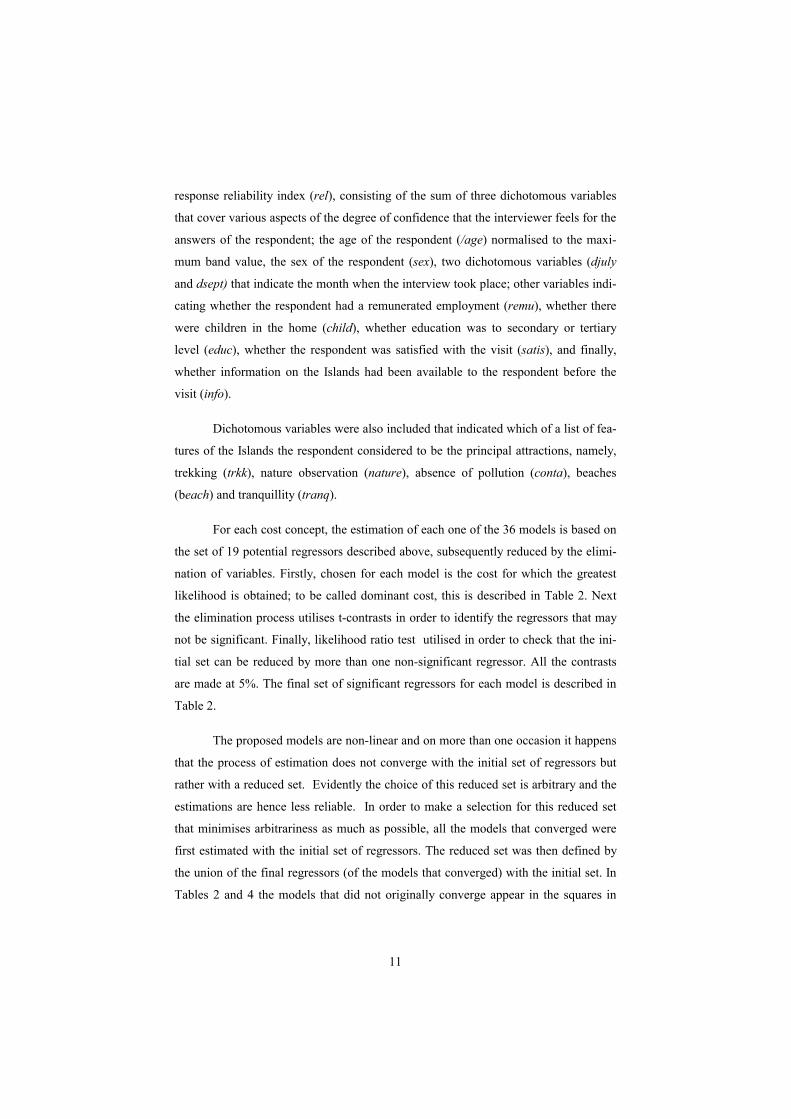
Table 2. Dominant cost and significant regressors

Displacement Total stay Model Non truncated Truncated In situ Non truncated Truncated In situ Poisson

ca beach tranq

know educ age

ca beach tranq know educ

age sex

ca beach tranq know educ

age

Dominate by the non truncated

NB2

Dominate by the truncated

NB2

Dominate by the In situ

NB2

BN2

Colapses to a non truncated

Poisson

Colapses to a truncated

Poisson

Colapses to a Poisson In

situ

ca beach know educ

age green info

ca (*) beach tranq

know

ca (*) beach tranq

know

LinLin

ca beach know

educ

Non con-vergence

Non con-vergence

ca know info

Non con-vergence

Non con-vergence

LinLog

cc beach tranq

know educ info

cc beach know

educ

Non con-vergence

cn dsept know

Non con-vergence

Non con-vergence

LogLin

ca beach know

educ age

ca beach know

educ age

ca beach know

educ age

ca beach know child

info

ca beach know

child

ca beach know

LogLog

ct beach tranq

know educ age info

ct beach tranq know educ

age info

Non con-vergence

ca beach know child

info

ca beach know

child

Ca (*) beach know

(*)These models only converge if the conditions for convergence are relaxed somewhat, and for the discrete models, if observations in respect of stays of more than 20 days are elimi-nated.

Of note is the fact that the dominant cost is ca, representing the sum of all the ex-

penses incurred by the visitor. It would therefore seem appropriate to avoid eliminating any

kind of expense from the cost definition. Of note also is the fact that income is at no time sig-

nificant, which would indicate that the recreational cost is separable from the other costs in

the individual utility function. Finally, the sets of significant regressors are quite similar be-

tween models, which would indicate that neither the specification nor the handling of the

sample is crucial for an understanding of which factors are determinants of demand.

Results in prediction terms

It is generally difficult to compare these models, since there is no contrast that would

compare them all. One way to compare the results of the different models is on the basis of

their predictions within the sample. Two measures can be used - the hit rate and the sum of

the squared residuals. For an observation xi we define a hit if the above-mentioned value is to

13

be located in the interval (xi – 0,5; xi + 0,5), in which case it would take the value 1 (and 0 if

outside the interval). The residual is defined simply as the difference between the model pre-

diction and the observation. The sum of squared residuals is therefore a measure of the dis-

tance between the prediction and the observation. Both rules are arbitrary, but they should

bring together the best part of the goodness of fit of the model. Table 4 describes the results

for the hit rate and the sum of squared residuals.

Calculated surpluses

The calculation of the surplus will depend on the model employed and is, in general,

the integral of expected demand (Table 1) from the current cost (sample mean, for example)

to the cut-off cost. In the Poisson and BN2 discrete models, the cut-off cost is by construction

infinite, since at any cost there is a probability, however small, of a positive demand. Table 3

describes the consumer surpluses for the six basic models described in Table 1. With the ex-

ception of the two discrete models, these formula change in accordance with the handling of

the sample, given that expected demand changes (see above). The notation is the same as in

Table 1.

Cuadro 3. Choke price and consumer surplus for basic models

Poisson, BN2: Choke price infinite

Consumer surplus - exp( + p) /

LinLin: Choke price cp = - /

Consumer surplus - 2 + 2 / 2 - p - p2 / 2

LinLog: Choke price cp = exp( - / )

Consumer surplus - exp( - / ) - p - (p ln p - p)

LogLin : Choke price cp = - ( + 2/2) /

Consumer surplus (1-exp( + p + 2 / 2)) /

LogLog: Choke price cp = exp( - ( + 2 / 2) / )

Consumer surplus

exp( + 2 / 2) ( exp[- ( + 2 / 2) ( + 1) / ] - p +1) / ( + 1) - exp[- ( + 2 / 2) / ] + p

Table 4 describes the surplus and cut-off cost estimations for each of the mod-

els, calculated for the sample mean of the regressors.

14

Table 4. Hit rate; sum of the squared residuals; expected consumer surplus; expected cut-off cost.5

Displacement Total stay Model Non truncated Truncated In situ Non truncated Truncated In situ

Poisson

59,4 % 758

41 350

72,5 % 671

1 695

71,2 % 671 750

Dominate by the non

truncated BN2

Dominate by the trun-cated BN2

Dominate by the In situ BN2

BN2

Colapses to a non truncated

Poisson

Colapses to a truncated

Poisson

Colapses to a In situ Poisson

33,8 % 224 353 28 212

60 % 242 983

0

60 % 241 772

0

LinLin

44,2 % 1 158 < 0

49 238

Non con-vergence

Non con-vergence

0,4 % 283 489

< 0 25 647

Non con-vergence

Non con-vergence

LinLog

46,5 % 1 172

47 385 105 540

56,5 % 1 215 1 133 2 165

Non con-vergence

0,4 % 287 015 10 943 3 316

Non con-vergence

Non con-vergence

LogLin

81,9 % 1 288

122 059 87 286

81,9 % 1 289

109 947 79 965

80,4 % 1 264

(†) (†)

67,1 % 258 538 89 189 59 608

65,8 % 258 658 39 905 34 800

15,8 % 259 052

(†) (†)

LogLog

81,2 % 1 282

407 827 325 337

81,3 % 1 282

325 337 1 973 947

Non con-vergence

62,1 % 258 520 46 832

118 401

64,2 % 258 572 16 722 49 545

28,8 % 256 721

(†) (†)

(†) The consumer surplus and choke price are difficult to calculate, but in accordance with the hit rate and squared residual sum criteria, these models are eliminated.

The results in Table 4 are very dispersed, which would indicate little

robustness in the face of different specifications or handling of the sample. In accor-

dance with the criterion of the hit rate, we select the LogLin or LogLog models to ex-

plain the displacements. Nevertheless, the good results are associated with pecularities

of the sample; most of the predictions for these models are to be found around one -

even in cases in which the observed demand is much greater - whereas the observed

frequency of visits equal to one is 80%. In other words, with this sample a blind pre-

diction of one visit for any one observation would have a success rate of 80%. These

models perform less well than the discrete models when the criterion is the sum of the

squared residuals. In this case, the best models correspond to a truncated or even an in

situ handling for the displacements, and a non-truncated handling for the entire stay.

5 The truncated BN2 and in situ models for total stay had to be estimated after elimi-nating observations of greater than 20 days. Hence their hit rates and squared residual sums are not strictly comparable with other models. In order to make these more comparable, included in the prediction were the observations that had been eliminated for the estimation.

15

The total stay seems to be more difficult to explain than the displacements, in-

dicating perhaps, that the two aspects of demand (displacements and stay) should be

modelled separately and not together as modelled here. The table of the significant

regressors is convincing in this sense, given that overall, fewer regressors are needed

to explain the total stay than are needed to explain the number of displacements,

which would indicate the presence of additional noise. The convergence difficulties of

the discrete models with this endogenous variable is probably due to the fact that

some observations are very atypical (very much above the mean). These observations

should perhaps be excluded, but to do this would increase the arbitrariness of the re-

sults. For these reasons it seems preferable to model the recreational demand of an

area of nature in terms of displacements and without taking into account the stay.

Notable differences occur in the surplus estimation, depending on the handling

of the sample, the measurement of demand or the specification. It is fundamental

therefore to compare the results from various models before selecting a measure for

the consumer surplus.

From all the above observations it appears that the most reliable results are to

be obtained by discrete displacement models, where the handling of the sample is

critical for the calculation of the consumer surplus. In accordance with the criterion of

the sum of the squared residuals, we allow that truncation should be taken into ac-

count, but it is not clear whether to use a simple truncated model or an in situ model;

the difference in the surpluses is considerable. The decision between the two is made

on the basis of statistical rigour, which requires the structure of the sample to be re-

produced as faithfully as possible. On this basis, a Poisson in situ model is chosen.

4. Representative sample from a reference population

The alternative to sampling in situ is a simple random sample from a specific

population. The fundamental interest in recurring to such a sample is that non-visitors

provide information regarding zero demand behaviour, in other words, information

regarding the way in which visitor demand would be cancelled if the displacement

cost were to be increased. This idea depends crucially on the hypothesis that non-

visitors essentially manifest the same behaviour patterns as visitors, and the principal

reason that they do not visit is because the displacement cost is too high. However,

16

another possible reason for not visiting could be that non-visitors have a preference

structure that is different from that of visitors; in other words, even given a lower dis-

placement cost, they would still not be interested in a visit.

If this is the case, then it is evident that non-visitors prove nothing about visi-

tor behaviour as the cost of displacement increases, and therefore would not be of any

value in calculating the consumer surplus.

In theory, since the visitors may come from anywhere, the area of reference

for a representative sample set is potentially very large. For our particular case, this

meant excluding all the observations for visitors from outside the area of reference. It

was decided to restrict the sample to the province of Pontevedra, it being the area

from which the majority of visitors come. The representative sample was constructed

by complementing the observations that had been previously obtained for visitors

with observations for non-visitors resident in this province. Preliminary telephone in-

terviews were carried out in order to establish the visitor/non-visitor proportions for

the province. Next, from the number of visitors from Pontevedra, distributed in 3

zones in function of the level of visits, the number of interviews to non-visitors neces-

sary for a representative sample of this province was calculated.6

A sample set from Pontevedra province consisting of 180 observations was

thus made available. This sample is qualitatively different from that of the visitors in

that it is intended to be representative of Pontevedra. A Kolmogoroff-Smirnoff test

was applied to check that there was no difference between the sample and population

proportions for the age and sex variables. Likewise, the sample was layered in accor-

dance with the size of the municipality of residence (five sizes), with no significant

difference between this and the population.

We now approach the empirical verification of the hypothesis that visitors and

non-visitors have the same preference structure. The method is quite a classic in cer-

tain economic disciplines such as health economics (Cameron and Trivedi, 1998), but

is less frequently applied in environmental economics. Using the sample set of visi-

tors and non-visitors, two models of demand are compared. The first is a classical

6 For the technical details of the construction of this combined sample, see González et al. 2000.

17

survey model (for example, Poisson) for which the same preference structure is as-

sumed, and the non-visitors are simply zero demand governed by the same regressors

as visitor demand. The second is the hurdle model. In order to compare it with the

survey model, the same endogenous structure is imposed, but the model is divided

into two parts. The first part is a discrete choice model in which the probability that a

person in the sample is a visitor; in the second part a truncated model is calculated,

explaining the number of visits to the park as conditional on having visited it, as in the

previous section. The comparison consists of assessing the two models in terms of

which explains the data better (greater verisimilitude); if it is the first, then the same

factors explains both the zeros and the positive demand numbers; and if it is the sec-

ond, then the decision to visit is qualitatively different from that of the number of

journeys. In this latter case, non-visitors are not simply potential visitors who consider

the displacement cost to be excessively high, and therefore, the calculation of the con-

sumer surplus should be made only on the basis of the truncated model.

Given the results obtained for the visitors in the previous section, only discrete

models are used, namely, Poisson and BN2. The set of the potential regressors is dif-

ferent from that for visitors since some of the variables are not defined for non-

visitors. The most important of these is the subjective cost of a journey to the islands,

which was substituted with the distance (km) from the home to the ferry port. The

variable conoc/know, referring to knowledge of the Islands, is defined for non-

visitors, with the difference that these have not directly experienced those aspects but

only know of their existence. The info variable - indicating whether the visitor had

access to information on the Islands prior to the visit - is converted for non-visitors to

whether they had ever received any information. The set of potential regressors re-

maining the same for the two samples are sex, rel, remu, educ, green, child, trkk, na-

ture, conta, beach, tranq and income. All non-dichotomous variables are normalised

via division by their respective maxima in the sample set, in order to speed up the es-

timation process.

Unfortunately, none of the two specifications converge with the set of all the

possible explanatory variables. Elimination, however, of the two variables referring to

18

the attractive features of the Islands – trekking and nature – permit the convergence.7

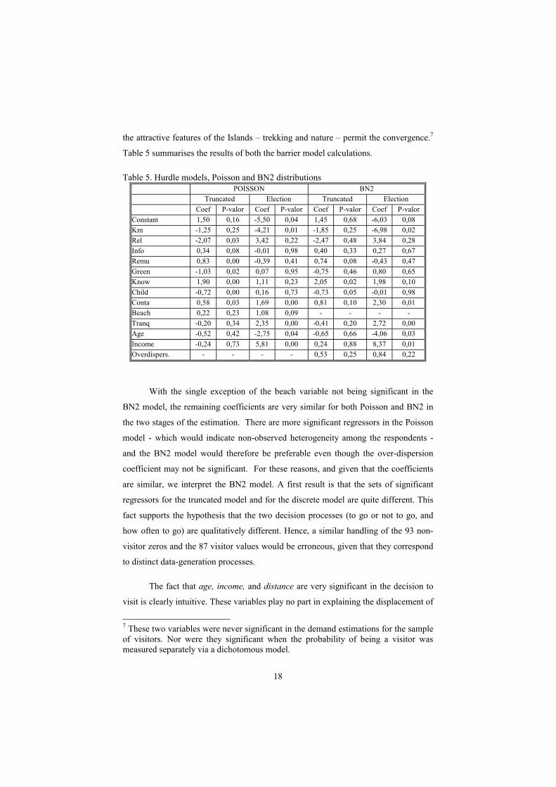
Table 5 summarises the results of both the barrier model calculations.

Table 5. Hurdle models, Poisson and BN2 distributions POISSON BN2

Truncated Election Truncated Election

Coef P-valor Coef P-valor Coef P-valor Coef P-valor

Constant 1,50 0,16 -5,50 0,04 1,45 0,68 -6,03 0,08

Km -1,25 0,25 -4,21 0,01 -1,85 0,25 -6,98 0,02

Rel -2,07 0,03 3,42 0,22 -2,47 0,48 3,84 0,28

Info 0,34 0,08 -0,01 0,98 0,40 0,33 0,27 0,67

Remu 0,83 0,00 -0,39 0,41 0,74 0,08 -0,43 0,47

Green -1,03 0,02 0,07 0,95 -0,75 0,46 0,80 0,65

Know 1,90 0,00 1,11 0,23 2,05 0,02 1,98 0,10

Child -0,72 0,00 0,16 0,73 -0,73 0,05 -0,01 0,98

Conta 0,58 0,03 1,69 0,00 0,81 0,10 2,30 0,01

Beach 0,22 0,23 1,08 0,09 - - - -

Tranq -0,20 0,34 2,35 0,00 -0,41 0,20 2,72 0,00

Age -0,52 0,42 -2,75 0,04 -0,65 0,66 -4,06 0,03

Income -0,24 0,73 5,81 0,00 0,24 0,88 8,37 0,01

Overdispers. - - - - 0,53 0,25 0,84 0,22

With the single exception of the beach variable not being significant in the

BN2 model, the remaining coefficients are very similar for both Poisson and BN2 in

the two stages of the estimation. There are more significant regressors in the Poisson

model - which would indicate non-observed heterogeneity among the respondents -

and the BN2 model would therefore be preferable even though the over-dispersion

coefficient may not be significant. For these reasons, and given that the coefficients

are similar, we interpret the BN2 model. A first result is that the sets of significant

regressors for the truncated model and for the discrete model are quite different. This

fact supports the hypothesis that the two decision processes (to go or not to go, and

how often to go) are qualitatively different. Hence, a similar handling of the 93 non-

visitor zeros and the 87 visitor values would be erroneous, given that they correspond

to distinct data-generation processes.

The fact that age, income, and distance are very significant in the decision to

visit is clearly intuitive. These variables play no part in explaining the displacement of

7 These two variables were never significant in the demand estimations for the sample of visitors. Nor were they significant when the probability of being a visitor was measured separately via a dichotomous model.

19

those who visit the nature area; on the other hand, child, remu and know play an im-

portant part in the number of displacements but not in the decision to visit. The only

factor which continues to be significant both in the decision to visit and in the number

of visits is the absence of pollution (conta), an important feature of the Islands. Fi-

nally, the other regressors do not play a clear role in the two decisions modelled here.

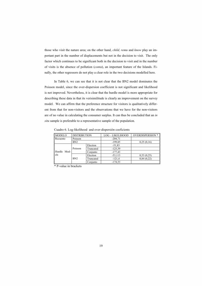
In Table 6, we can see that it is not clear that the BN2 model dominates the

Poisson model, since the over-dispersion coefficient is not significant and likelihood

is not improved. Nevertheless, it is clear that the hurdle model is more appropriate for

describing these data in that its verisimilitude is clearly an improvement on the survey

model. We can affirm that the preference structure for visitors is qualitatively differ-

ent from that for non-visitors and the observations that we have for the non-visitors

are of no value in calculating the consumer surplus. It can thus be concluded that an in

situ sample is preferable to a representative sample of the population.

Cuadro 6. Log-likelihood and over-dispersión coeficients

MODELO DISTRIBUTION LOG – LIKELIHOOD OVERDISPERSION * Poisson -204,71 Recuento BN2 -199,85 0,25 (0,16)

Election -51,83 Truncated -125,59

Poisson

Conjunto -177,43 Election -53,113 0,53 (0,25) Truncated -121,4 0,84 (0,22)

Hurdle Mod-els

BN2 Conjunto -174,53

* P-value in brackets

20

5. Conclusions

With respect to the objectives laid down in the introduction, the best demand

prediction results were obtained with an in situ sample, with a truncated or in situ

treatment of the sample, with an average demand defined in terms of number of visi-

tors to the area of nature, and with a displacement cost that includes all the costs in-

curred in the visit. The variation in results in terms of the consumer surplus would in-

dicate the importance of making comparisons between various demand models.

We feel unable to make a judgement in respect of truncated handling versus in

situ handling of the sample. This is probably due to the peculiarities of our sample;

the majority of visitors made just one visit in five years, and therefore the truncation

effect is more important for describing the sample than the frequency modifications of

the higher visit numbers. In other words, the in situ handling supplies to the estima-

tion process the information that the sample is truncated (which is the essential infor-

mation). The fact that it corrects, in addition, the frequencies of the higher visit num-

bers changes the demand configuration only marginally. Hence it is quite possible that

in other samples in which the proportion of one-time visitors is less important, in situ

handling might obtain better predictions than truncated handling. In the same way,

the number of visits in this sample is characterised by equi-dispersion (a variance ap-

proximately equal to the mean), and it is therefore only to be expected that the nega-

tive binomial distribution does not obtain better results than the Poisson distribution.

For a sample not characterised by equi-dispersion, it is quite possible for the results

obtained here to be reversed. Again, these issues highlight the importance of compar-

ing different kinds of models.

Finally, it was proven that non-visitors may have a preference structure that is

qualitatively different from that of visitors, and that therefore, when estimating a con-

sumer surplus for the demand for an area of nature, only one sample is necessary.

21

References

BELL F.W. y LEEWORTHY V.R. (1990): “Recreational demand by tourists for saltwater beach days”. Journal of Environmental Economics and Management, 18, pp. 189-205.

CAMERON T.A. y TRIVEDI P. (1998): Regression analysis of count data. Cam-bridge University Press.

CAMPOS P., RIERA, P., DE ANDRÉS R., y URZAINQUI E. (1996): “El valor eco-nómico total de un espacio de interés natural. La dehesa del área de Monfragüe” en Azqueta, D., Pérez y Pérez, L. (1996): Gestión de espacios Naturales. La demanda de servicios recreativos. McGrawHill.

DEL SAZ S. Y PEREZ L.(1999): “Estimación de los beneficios del uso recreativo del parque de L’Albufera con el método indirecto de los costes de viaje”. Revista de Estudios de Economía Aplicada, nº 11, pp. 41-62.

DOBBS I.M. (1993): “Individual travel cost method: estimation and benefits assess-ment with discrete and possibly gouped dependent variable”. American Journal of Agricultural Economics, 75, pp. 84-94.

ENGLIN J.E. y LAMBERT D. (1995): “Measuring angling quality in count data models of recreational fishing: a non tested test of three approaches”. Environ-mental and Ressource Economics, 6, pp. 389-399.

ENGLIN J.E. y SHONKWILER J.S. (1995) “Estimating social welfare using count data models: an application to long run recreational demand under conditions of endogenous stratification and truncation”. The Review of Economics and Statis-tics, 77 (1), pp. 104-112.

FARRÉ M. (1998): Economía Política dels Espais Naturals Protegits. Estudi D’un Cas Concret: El Parc Nacional D’Aigüestortes i Estan-y de Sant Maurici. Tesis Doctoral, Departament d’Economía Aplicada, Facultat de Dret i Economía, Universitat de Lleida.

GARRIDO A. GOMEZ-LIMON J. DE LUCIO J.V. y MUGICA M. (1996) “Estudio del uso y valoración del parque regional de la Cuenca Alta del Manzanares (Madrid) mediante el MCV”, en Azqueta, D., Pérez y Pérez, L. (1996): Gestión de espacios Naturales. La demanda de servicios recreativos. McGrawHill.

GONZALEZ M. (1997) “Valoración Económica del uso recreativo-paisajístico de los montes: aplicación al parque natural del Monte Aloia en Galicia”. Tesis Docto-ral. Microfichas nº 76. Universidade de Vigo.

GONZALEZ M. (2000) “As funcións ecolóxico-ambientais do monte en Galicia: unha perspectiva económica”. Servicio de Publicacións da Diputación Provin-cial de Pontevedra.

GONZALEZ M., POLOME P. y PRADA A. (2000) “Entrevistas a visitantes a un espacio natural con gestión pública: sesgos sobre la información obtenida y la estimación de beneficios”. Documento de traballo número 0008. Departamento de Economía Aplicada. Universidade de Vigo.

GONZALEZ M., GONZALEZ X., POLOME P., PRADA, A. VAZQUEZ, M. (2000): Valoración Económica del Patrimonio Natural. Series Monográfica del

22

Instituto de Estudios Económicos de Galicia “Fundación Pedro Barrié de la Ma-za”, A Coruña.

GREENE W. H. (1998): Análisis Econométrico. 3º edición, Prentice Hall, Madrid.

HANLEY N. (1989): “Valuing rural recreational benefits: an empirical comparision of two approaches”. Journal of Agricultural Economics, 40 (3), pp. 361-374.

HELLERSTEIN D.(1991): “Using count models in travel cost analysis and other de-mand models”. Water Ressources Research, 28 (8). 1999-2004.

HELLERSTEIN D. y MENDELSOHN R. (1993): “A theoretical foundation for count data models”. American Journal of Agricultural Economics, 75, pp. 604-611.

PÉREZ L, BARREIRO J., BARBERAN R. y DEL SAZ S.(1998): “El parque Posets-Maladeta. Aproximación económica a su valor de uso recreativo”. Consejo de Protección de la Naturaleza de Aragón.

RANDALL A. (1994) “A difficulty with the travel cost method”. Land Economics, 70, pp. 80-96.

RIERA P., DESCALZI C., RUIZ A. (1994): “El valor de los espacios de interés natu-ral en España. Aplicación de los métodos de la valoración contingente y el coste del desplazamiento”. Revista Española de Economía, pp. 207-230.

SANTOS SILVA J.J.C. (1997): “Unobservables in Count Data Models for On-Site Samples”. Economic Letters, 54, pp. 217-220.

SHAW D. (1988): “On-Site Samples’ Regression. Problems of Non-Negative Inte-gers, Truncation and Endogenous Stratification”. Journal of Econometrics, 37, pp. 211-233.

WILLIS K. Y GARROD G. (1991): “An individual travel cost method of evaluating forest recreation”. Journal of Agricultural Economics, 42, pp. 33-42.

23

Appendix 1: Consumer surplus for the Poisson or BN2 models with costs ex-pressed in logarithms

Proposition. In a Poisson or BN2 model with expectation = exp( + ln p), where and are parameters and p is the cost, the consumer surplus is infinite except for

values of less than -1.

Proof. The surplus (EC/CS) of a consumer having such expected demand is

EC = p dpXYE | = p dttlnexp = p dtte

= 1/11 pe = > -1.

Appendix 2: Definitions of displacement costs

On the basis of the following costs, seven displacemement costs are defined:

Table 7. Costs incurred (respondent estimations) 1. TIM1: Length of return journey from home to temporary residence in Galicia 2. C1: Cost per person per return journey from home to temporary residence 3. DOUT: Number of days spent away from home 4. COUT: Cost per person per day for accomodation These 4 variables were always zero for visitors who went directly from home to the ferry port of the Cíes Islands. 5. TIM2: Length of return journey from home to ferry port 6. C2: Cost per person per return journey from home to ferry port 7. CB: Cost of return ferry boat journey to the Islands 8. DISL: Number of days spent on the Islands 9. CISL: Cost per person per day for the stay on the Islands (in excess of 1 day) Auxiliary to cost variables: Disf: Dichotomous variable indicating whether the visitor considers the journey in (5) to be enjoyable Mot: Dichotomous variable indicating whether the main reason for being in the Autonomous Community of Galicia is the journey to the Islands Ca Total cost, including nights of arrival and departure = ( (Tim1*1063 + C1) / DOut + 2*COut + (Tim2 + 2)*1063 + C2 + CB ) / DIsl1 + CIsl

Cn Does not take into account nights spent away from the Islands = ( (Tim1*1063 + C1) / DOut + (Tim2 + 2)*1063 + C2 + CB ) / DIsl1 + CIsl

Cc Displacement from home to ferry port is only a cost for those who declare it so = ( (Tim1*1063 + C1) / DOut + 2*COut + (1 - disf)*(Tim2 + 2)*1063 + C2 + CB ) / DIsl1 + CIsl

24

Cd The length of stay on the Islands is irrelevant (these can be visited in a day) = (Tim1*1063 + C1) / DOut + 2*COut + (Tim2 + 2)*1063 + C2 + CB

Ct The opportunity cost of time is null (Spanish labour market inflexibility) = ( C1 / DOut + 2*COut + C2 + CB ) / DIsl1 + CIsl

Cm The cost of getting to the temporary residence (Tim1, C1, COut) is only counted for those visitors whose principal motive for travelling is the visit to the Islands = ( Mot*( (Tim1*1063 + C1) / DOut + 2*COut ) + (Tim2 + 2)*1063 + C2 + CB ) / DIsl1 + CIsl

Tim, C The monetary and time costs are considered separately

Tim = Tim1 / DOut + Tim2 + 2 C = C1 / DOut + C2 + CB

DOCUMENTOS DE TRABALLO XA PUBLICADOS

ÁREA DE ANÁLISE ECONÓMICA: 1. Experimentación y estructura de mercado en la relación de licencia de patentes no drásticas. El caso

de información simétrica. (Manuel Antelo Suárez).

2. Experimentación y estructura de mercado en la relación de licencia de patentes no drásticas. El caso de información asimétrica. (Manuel Antelo Suárez).

3. Modelos empíricos de oligopolio: una revisión. (María Consuelo Pazó Martínez).

4. El Análisis económico de los procesos de urbanización. (Olga Alonso Villar).

5. Optimal Tariffs WhenProduction is fixed. (José Méndez Naya; Luciano Méndez Naya).

6. Reglas de clasificación discriminante: aplicación a la vivienda. (Raquel Arévalo Tomé).

7. Estructura demográfica y sistemas de pensiones. Un análisis de equilibrio general aplicado a la economía española. (María Montero Muñóz).

8. Spatial distribution of production and education. (Olga Alonso-Villar).

9. Diferencias salariales y comportamiento no competitivo en el mercado de trabajo en la industria española. (Víctor Manuel Montuenga, Andrés E. Romeu Santana, Melchor Fernández Fernández)

10. GPs’ Payment Contracts and their Referral Policy. (Begoña Garcia Mariñoso and Izabela Jelovac)

11. Una nueva matriz de contabilidad social para España: la SAM-90. (Melchor Fernández y Clemente Polo)

12. Money and Busines Cycle in a Small Open Economy. (Eduardo L. Giménez y José María Martín-Moreno).

13. Endogenous Growth With Technological Change: A Model Based On R&D Expenditure. (Mª Jesús Freire-Serén).

14. Productive Public Spending In A Balassa-Samuelson Model Of Dual Inflation. (Jóse María Martín-Moreno y Jorge Blázquez).

15. Efficient Allocation of Land between Productive Use and Recreational Use. (Eduardo L. Giménez, Manuel González Gómez).

16. Funcional Forms, Sampling Considerations and Estimation of Demand for Protected Natural Areas: The Cíes Islands Case Study in Galicia (Spain). (Manuel González Gómez, Philippe Polomé y Albino Prada Blanco).

ÁREA DE ECONOMÍA APLICADA:

1. Economía de Mercado e Autoxestión: Sociedades Anónimas Laborais do Sector Industrial en Galicia.

(Xosé Henrique Vazquez Vicente).

2. Fecundidade e Actividade en Galicia, 1970-1993. (Xoaquín Fernández Leiceaga.)

3. La reforma de la financiación autonómica y su incidencia en Galicia. (Xoaquín Álvarez Corbacho).

4. A industria conserveira: Análise económica dunha industria estratéxica en Galicia. 1996. (José Ramón García González).

5. A contabilización física dos fluxos de enerxía e materiais. (Xoan Ramón Doldán García).

6. Indicadores económico-financieiros estratificados do sector industrial conserveiro en galicia. 1993-1996.(José Ramón García González).

7. A desigualdade relativa na distribución persoal da renda en Galicia. Análise cuantitativa a partir dos

datos da EPF 90/91. (Ángela Troitiño Cobas).

8. O benestar-renda en Galicia. Análise cuantitativa a partir dos datos da EPF 90/91. (Ángela Troitiño

Cobas).

9. El fraccionamiento del periodo impositivo en el IRPF Español y la decisión temporal de casarse.

(Jaime Alonso, Xose C. Alvárez, Xose M. González e Daniel Miles)

ÁREA DE HISTORIA:

1. Aproximación ao crédito na Galiza do S. XIX. Os casos da terra de Santiago e da Ulla. (Francisco

Xabier Meilán Arroyo)

2. Aspectos do comercio contemporáneo entre España e Portugal. (Carmen Espido Bello).

3. Pensamento económico e agrarismo na primeira metade do século XX. (Miguel Cabo Villaverde).

4. Civilizar o corpo e modernizar a vida: ximnasia, sport e mentalidade burguesa na fin dun século. Galicia 1875-1900. (Andrés Domínguez Almansa).

5. Las élites parlamentarias de Galicia (1977-1996). (Guillermo Marquez Cruz).

6. Perfil do propietario innovador na Galicia do século XIX. Historia dun desencontro. (Xosé R. Veiga Alonso).

7. Os atrancos do sector pecuario galego no contexto da construcción do mercado interior español, 1900-1921. (Antonio Bernardez Sobreira).

8. Los estudios electorales en Galicia: Una revisión bibliográfica (1876-1997). (Ignacio Lago Peñas).

9. Control social y proyectos políticos en una sociedad rural. Carballo, 1880-1936. (Silvia Riego Rama.

ÁREA DE XEOGRAFÍA:

1. A industria da lousa. (Xosé Antón Rodríguez González; Xosé Mª San Román Rodríguez).

2. O avellentamento demográfico en Galicia e as súas consecuencias. (Jesús M. González Pérez; José Somoza Medina).

3. Estructura urbana da cidade da coruña, os barrios residenciais: o espacio obxetivo e a súa visión a través da prensa diaria. (Mª José Piñeira Mantiñán; Luis Alfonso Escudero Gómez).

4. As vilas e a organización do espacio en Galicia. (Román Rodríguez González).

5. O comercio nas cabeceiras do interior de Galicia. (Alejandro López González).

6. A mortalidade infantil no noroeste portugués nos finais do século XX. (Paula Cristina Almeida Remoaldo).

7. O casco histórico de Santiago de Compostela, características demográficas e morfolóxicas. (José Antonio Aldrey Vázquez; José Formigo Couceiro).

8. Mobilidade e planificación urbana en santiago de compostela: cara a un sistema de transportes sustentable. (Miguel Pazos Otón).

9. A producción de espacio turístico e de ocio na marxe norte da ría de pontevedra.(Carlos Alberto Patiño Romarís)

ÁREA DE XESTIÓN DA INFORMACIÓN

1. Estudio Comparativo das Bases de Datos: Science Citation Index, Biological Abstracts, Current contents, Life Science, Medline. (Margarida Andrade García; Ana María Andrade García; Begoña Domínguez Dovalo)

2. Análise de satisfacción de usuarios cos servicios bibliotecarios da Universidade na Facultade de Filosofía e CC. da Educación de Santiago. (Ana Menéndez Rodríguez; Olga Otero Tovar; José Vázquez Montero).

Tódolos exemplares están dispoñibles na biblioteca do IDEGA, así como na páxina WEB do Instituto(http://www.usc.es/idega/)

NORMAS PARA A REMISIÓN DE ORI INAIS:

e er n ser re i idos res e e lares do ra allo e un a co ia en dis e e ao irec or do vda. das ciencias s/n . a us Universi ario ur. 06 an iago de o os ela cu rindo coas seguin es nor as

. ri eira ina de er incluir o ulo o/s no e/s enderezo/s el ono/s

correo elec r nico e ins i uci n/s s ue er ence o/s au or/es un ndice ala ras c ave ou descri ores as co o dous resu os dun i o de

200-2 0 ala ras un na l ngua na ue es ea escri a o ra allo e ou ro en ingl s.

2. e o es ar en in erlineado con ar es ni as de res cen e ros e cun a e ensi n i a de cincuen a olios inclu das as no as e a

i liogra a. 3. i liogra a se resen ar al a e ica en e ao inal do e o seguindo o

odelo elidos e iniciais do au or en aiusculas ano de u licaci n en re ar n ese e dis inguindo a c en caso de is dun a o ra do es o

au or no es o ano. ulo en cursiva. s ulos de ar igo ir n en re as as e os no es doas revis as en cursiva. lugar de u licaci n e edi orial en caso de li ro e en caso de revis a volu e e n de revis a seguido das

inas inicial e inal unidas or un gui n. . s re erencias i liogr icas no e o e nas no as ao seguir n os odelos

a i uais nas di eren es es ecialidades cien icas. . so or e in or ico e regado de er ser ord ice ara indo s

cell ou cces. 6. direcci n do acusar reci o dos ori inais e resolver so re a s a

u licaci n nun razo rudencial. er n re erencia os ra allos resen ados s esi ns ien icas do ns i u o.

so e er dolos ra allos reci idos a avaliaci n. er n cri erios de

selecci n o nivel cien ico e a con ri uci n dos es os an lise da realidade socio-econ ica galega.