analyses of assumptions and errors in the calculation of ... pdf/ewers...represents sap flux in the...

Summary We analyzed assumptions and measurement er-rors in estimating canopy transpiration (EL) from sap flux (JS)measured with Granier-type sensors, and in calculating canopystomatal conductance (GS) from EL and vapor pressure deficit(D). The study was performed in 12-year-old Pinus taeda L.stands with a wide range in leaf area index (L) and growth rate.No systematic differences in JS were found between the northand south sides of trees. However, JS in xylem between 20 and40 mm from the cambium was 50 and 39% of JS in the outer20-mm band of xylem in slow- and fast-growing trees, respec-tively. Sap flux measured in stems did not lag JS measured inbranches, and time and frequency domain analyses of time se-ries indicated that variability in JS in stems and branches ismostly explained by variation in D. Therefore, JS was used toestimate transpiration, after accounting for radial patterns.There was no difference between D and leaf-to-air vapor pres-sure gradient, and D did not have a vertical profile in stands ofeither low or high L suggesting a strong canopy–atmospherecoupling. Therefore, D estimated at one point in the canopy canbe used to calculate GS in such stands. Given the uncertaintiesin JS, relative humidity, and temperature measurements, tokeep errors in GS estimates to less than 10%, estimates of GS

should be limited to conditions in which D ≥ 0.6 kPa.

Keywords: air temperature, air vapor pressure deficit, leaftemperature, leaf-to-air vapor pressure deficit, relative hu-midity, time lags.

Introduction

Stomata respond to environmental variation, regulate waterloss and carbon dioxide gain, and thus biosphere–atmosphereexchange of mass and energy. From porometry measure-ments, leaf conductance (gS) can be calculated with Fick’s lawas:

gS = EL

wδ, (1)

where EL is transpiration per unit leaf area (mol m–2 s–1), and

δW (mol mol–1) is the water vapor pressure gradient betweenthe substomatal cavity and the air near the leaf surface (Pearcyet al. 1989). Mean gS of the canopy (<gS>; mol m–2 s–1)(Sellars et al. 1997, Baldocchi and Meyers 1998, Pataki et al.1998a), can be obtained from measurements of gS at severallevels in the canopy, together with the vertical distribution ofleaf area, and models describing stomatal responses to envi-ronmental gradients within the canopy (Jarvis 1995). How-ever, variation among porometric measurements of gS is large(Jarvis 1995, Hinckley et al. 1998). Leverenz et al. (1982) cal-culated that, in a uniform monospecific Norway spruce can-opy, the number of sample leaves needed to produce anestimate within 10% of the mean at each time step may exceed150 even if sampling is stratified by major sources of varia-tion.

Recently, <gS> has been approximated from sap flux (JS)measurements scaled to EL (Köstner et al. 1992, Arneth et al.1996, Granier et al. 1996, Martin et al. 1997, Oren et al. 1998,Pataki et al. 1998a, 1998b, Phillips and Oren 1998, Oren et al.1999a). When leaf and air temperature are similar, a conditionthat occurs for small leaves exposed to a sufficiently high windspeed (Herbst 1995, Martin et al. 1999), the bulk air vaporpressure deficit (D) can be used as an approximation of δW forcalculating gS (Monteith and Unsworth 1990). Under suchconditions, calculation of <gS> from sap-flux-scaled EL (here-after, GS) can be simplified as suggested by Monteith andUnsworth (1990):

GS = K T E

DG A L( )

, (2)

where GS is mean canopy stomatal conductance to water vapor(m s–1), KG is the conductance coefficient as a function of tem-perature (115.8 ± 0.4236 kPa m3 kg–1)—accounting for tem-perature effects on the psychrometric constant, latent heat ofvaporization, specific heat of air at constant pressure, and thedensity of air—and TA is bulk air temperature (°C). Phillipsand Oren (1998) showed that errors associated with lumpingthe temperature-dependent physical coefficients into KG arenegligible.

Tree Physiology 20, 579–589© 2000 Heron Publishing—Victoria, Canada

Analyses of assumptions and errors in the calculation of stomatalconductance from sap flux measurements

BRENT E. EWERS1,2 and RAM OREN1

1 Nicholas School of Environment, Duke University, Durham, NC 27708-0328, USA2 Present address: University of Wisconsin, Department of Forest Ecology and Management, 120 Russell Laboratories, 1630 Linden Dr., Madison,

WI 53706, USA

Received June 4, 1999

Because sap-flux-scaled GS is the product of measurementsrepresenting relatively large leaf areas, it is subject to certainsources of error. These include errors in estimating EL and δW

because of systematic and random variations and instrumentlimitations. This study was designed to generate a conditionalsampling scheme aimed at keeping the effect of measurementerrors in the estimate of GS to within 10% of the measurementerror-free estimate.

Errors in estimating EL

Sap-flux-scaled EL may represent water uptake rather thantranspiration if the quantity of water discharged from storagein the plant into the transpiration stream in the morning is largerelative to uptake, and the quantity recharged by uptake late inthe day is large relative to transpiration (Granier et al. 1996,Phillips et al. 1996, Loustau et al. 1998, Phillips and Oren1998). To assess if JS can be used to calculate GS in this stand,we evaluated the effect of stem water storage capacity on EL

by comparing a time series of stem JS measured with Granier-type sensors with branch JS measured with Kuèera-type sen-sors (Cienciala et al. 1994) in the top and bottom branches ofthe canopy.

Increasingly, sap flux in the hydroactive xylem is estimatedwith Granier-type sensors (Granier 1987), which measure themaximum temperature difference between heated and un-heated probes during times of zero flux (∆TM) as a baseline.Temperature difference (∆T) is also measured during the dayas water carries heat away from the probe. Deviation from thebaseline is used to estimate water flux. Granier-type sensorsmay be sensitive to temperature gradients in the stem creatingan apparent temperature difference (Goulden and Field 1994,Köstner et al. 1998). This error can be large when fluxes arelow, and trees are small (Granier 1987). Additional errors,even in large trees, may be caused by uncertainties in the base-line position (i.e., ∆TM). Therefore, we quantified the effect ofuncertainties in ∆TM on estimates of diurnal time courses of JS.

Errors in estimating δW

Calculation of D requires measurements of relative humidityof bulk air (RH), and TA, and calculations of δW require addi-tional measurements of leaf temperature (TL; °C). It is oftenassumed that a single sensor is sufficient to represent D in thecanopy (Köstner et al. 1992, Granier et al. 1996, Martin et al.1997, Oren et al. 1998, Pataki et al. 1998a, 1998b). Forwell-coupled canopies at sufficiently high wind speeds, D ap-proximates δW (Jarvis and McNaughton 1986, Martin et al.1999), and thus a single RH–TA sensor can be used to calculateGS. In this study, we analyzed the effects of measurement er-rors on values of δW and D and, in turn, on the calculation ofGS. We also tested the assumption that D does not vary hori-zontally and vertically by performing: (1) concurrent measure-ments in nearby stands with twofold difference in leaf areaindex (L) and an adjacent opening, and (2) rapid measure-ments along a vertical transect within the canopy.

Material and methods

Study site and treatments

The Southeast Tree Research and Education Site (SETRES)was established in 1992 in a stand of Pinus taeda L. planted in1984 in the Sandhills of North Carolina (35° N, 79° W) on aninfertile, well-drained, sandy, siliceous, thermic PsammenticHapludult soil (Wakulla series). Mean annual precipitation is1210 mm with occasional growing season water deficits.Three treatments were established in addition to a control (C):irrigated (I), fertilized (F), and a combination of irrigation andfertilization (IF). Nutrient treatments have been maintainedsince March 1992 and irrigation treatments since April 1993.The treatments have resulted in peak L of 1.8, 1.9, 3.3, and 3.6and basal areas of 14, 14, 20, and 25 m2 ha–1 for trees in the C,I, F, and IF treatments, respectively. For details of nutritionand irrigation treatments see Albaugh et al. (1998) and Murthyet al. (1996).

Stem JS and associated environmental variables were mea-sured from August 1996 to January 1999. During this period,short measurement campaigns were carried out to evaluate po-tential sources of error.

Sap flux measurements

We measured JS in stem xylem of eight trees in a 6-m diameterplot and in branch xylem in a subset of three trees within eachtreatment (Ewers et al. 1999). Measurements on the north sideof stems (1.4 m above ground) were made with Granier-typesensors at two depths: the outer 20 mm of the xylem (JSout) ineight trees, and, to account for radial patterns in JS, the next20 mm of the xylem (JSin) in a subset of five trees. The JS (m3

H2O m–2 s–1) is calculated based on the empirical equation(Granier 1987):

JS = × −

−119 10 6

1 231∆ ∆∆

T T

TM

.

. (3)

We calculated mean JS, weighting JSout by the sapwood arearepresented in that xylem band and JSin by the sapwood areainternal to the outer band (Ewers et al. 1999), assuming thatJSin represents sap flux in the xylem between 20 and 40 mmfrom the cambium. On average, sapwood area inside the outer20-mm band was 15% of the total. On June 12–24, 1998, toevaluate whether scaling must account for a systematic cir-cumferential variance in flux, we installed sensors to measureJSout on the south side of stems of a subset of five trees in C andIF, and compared these with measurements made on the northside. Trees in the C and IF treatments were chosen becausethey represented the highest and lowest L and differed in sap-wood characteristics (Ewers et al. 1999).

We evaluated time lags between water uptake and transpira-tion by measuring xylem flux with Kuèera-type sensors (Cien-ciala et al. 1994), based on the heat balance method, in upperbranches of 6–12 mm diameter and lower branches of12–18 mm diameter. Branch measurements were made from

580 EWERS AND OREN

TREE PHYSIOLOGY VOLUME 20, 2000

July 23 to August 8, 1998. To avoid thermal gradients from di-rect radiation, all sensors were shielded. Analyses of daily wa-ter use were performed on daily sums of JS from 0500 to0500 h, corresponding approximately to the time of zero flow,and therefore include nighttime recharge (Phillips and Oren1998).

To calculate EL (kg H2O m–2 AL s–1), JS (kg H2O m–2 AS s–1)for either branches or stems is combined with sapwood area(AS; m2) and leaf area (AL; m2) as follows (Pataki et al. 1998b):

EL = JSA

AS

L

. (4)

Environmental measurements

Values of δW were calculated from RH, TL, and TA based onequations adapted from Goff and Gratch (1946):

V e T TS

L L= +0 611 17 27 237. ( . ) ), (5)

δWH

S S=

−R

V V100

, (6)

where VS is saturated water vapor pressure (kPa). Here, δW isin kPa and can be converted to mole fractions used in Equa-tion 1 by dividing by atmospheric pressure. The value of D iscalculated from Equations 5 and 6, where TA is substitutedfor TL.

During most of the study period, an RH–TA probe (VaisalaHMP 35C, Campbell Scientific, Logan, UT) was positioned atthe center of each plot at 2/3 distance from the bottom of thecanopy (sensor height/stand height, z/h = 0.79–0.83). DuringAugust 2–28, 1997, additional measurements of TL weremade in each treatment by infrared thermometry (EverestInterscience, Palo Alto, CA) based on an emissivity of 0.97(Gates 1965, Gay and Knoerr, 1975). We used these measure-ments to test the validity of replacing D with δW for calculatingGS. We also used the measurements to assess the effect of hori-zontal variability in L on D. On July 23 and August 5, 1998,the effect of the vertical distribution of leaf area on the D pro-file was evaluated by raising and then lowering the sensor 1 mmin–1 during the midday plateau in the diurnal pattern of D.

Photosynthetic photon flux density (Q) above the canopywas monitored with a quantum sensor (LI-190s, Li-Cor, Lin-coln, NE). Xylem flux and all environmental sensors weresampled every 30 s (DL2, Delta-T Devices, Cambridge,U.K.). Thirty-minute mean values were recorded during thestudy, except for branch JS for which 15-min averages were re-corded.

Structural measurements

At the end of the study, branches monitored for sap flux wereharvested. No heartwood was visible in upper or lowerbranches, but the pith was clearly discernible from the sap-wood. Branch sapwood area was determined by subtractingthe bark and heartwood areas from the branch cross-sectional

area at the midpoint of sensor length. From each branch, fivefascicles were selected randomly from current- and previ-ous-year foliage. The length and width of each needle weremeasured to ± 1 and ± 0.005 mm, respectively. Projected leafarea was determined by multiplying the width of each needleby its length and then summing the area for the fascicle. Need-les were then oven-dried for at least 24 h at 65 °C, weighed,and their specific leaf area (cm2 g–1) determined. The remain-ing needles of each age class were also oven-dried. Total leafarea of each branch was obtained by multiplying leaf mass ineach age class by the respective specific leaf area and sum-ming the area of both age classes.

Heartwood was not present in any stems of any treatmentsas expected for P. taeda of this age (cf. Megraw 1985). There-fore, sapwood area for each tree was calculated from diameterat sensor height. Bark thickness was measured in each tree anddiffered among treatments (Ewers et al. 1999). After correct-ing for bark thickness, sapwood area per unit of ground areawas calculated by summing the area of all trees in the plot anddividing by plot area. Sapwood area was 9.0, 9.0, 15.2,21.9 m2 ha–1 for trees in the C, I, F, and IF treatments, respec-tively (Ewers et al. 1999). Leaf area of each tree was cal-culated from allometric relationships derived from winterbiomass harvests at the site (Albaugh et al. 1998). Leaf areaestimates for each tree were corrected for seasonality based onrelative increase in leaf area from winter to the sampling pe-riod as determined with a leaf area meter (Li-Cor, LAI-2000)and litterfall at the stand level (Ewers et al. 1999). The AS:AL

ratio was calculated for each tree based on estimates of leafarea and sapwood area. To estimate stand L (projected), “win-ter equivalent” leaf area of each tree in each subplot was esti-mated from its diameter and the treatment specific allometricrelationships as above (Albaugh et al. 1998, Ewers et al.1999). Leaf area measurements of all individuals in each sub-plot were summed, divided by the plot area (133 m2) and cor-rected for seasonal leaf area dynamics.

Statistical analyses

All statistical analyses were made with SAS procedures GLM,ARIMA and SPECTRA (Version 6.12, SAS Institute, Cary,NC). Nonlinear curve fits were performed in SIGMAPLOT(Version 4.5, SPSS, San Rafael, CA). Time lags were evalu-ated by time series analyses performed both in the time andfrequency domain according to Brocklebank and Dickey(1986).

Results

Errors in estimates of JS caused by baseline placement

Occasionally, an apparently stable ∆TM became unstable inearly morning when sap flux began. We chose the most unsta-ble behavior found among all trees as an example in Figure 1.Relatively stable ∆TM (defined as the portion of ∆TM that var-ies within the narrow range of 0.02 mV for at least 2 h) is plot-ted alongside unstable ∆TM (defined as the ∆TM connecting the

TREE PHYSIOLOGY ON-LINE at http://www.heronpublishing.com

ERRORS IN SAP-FLUX-SCALED STOMATAL CONDUCTANCE 581

greatest temperature differences). The maximum differencebetween stable and unstable ∆TM values occurred on June 16and amounted to 0.1 °C, a small fraction of the mean ∆TM of

12 °C.The effect of the difference between stable and unstable

∆TM (Figure 1) on the absolute value of JS was very small (Fig-ure 2A). However, even a small error in ∆TM placement maycause large errors in estimates of GS under conditions of lowsap flux. The effect of ∆TM placement on errors in JS (and thusEL and GS) was assessed by normalizing the difference be-tween JS estimated with stable and unstable ∆TM by the valuesobtained with the stable ∆TM, and relating this relative error inJS to D (Figure 2B).

Azimuthal and radial patterns in stem JS

The JSout in south-facing sensors was a constant proportion ofJSout in north-facing sensors along the entire range of D, butwas highly variable at low D (Figure 3). In both the C and IFstands, the ratio of JS measured toward the south relative tothat measured toward the north was unity (paired t-test P =0.88), even after reducing the variability by selecting data cor-responding to D ≥ 0.6 kPa. Therefore, the daily sum of JS wassimilar in both directions (P = 0.86). Furthermore, the ratio ofnorth to south JS was similar in both stands (P = 0.50).

We quantified the fertilization-induced increases in L andgrowth rate on the radial change in JS between the outer 20mm and the next 20 mm in the xylem. In both the C and IFstands, the JSin/JSout ratio was constant with respect to D. How-ever, the daily sums of JSin and JSout differed (P = 0.001). In theslow-growing C stand, JSin was 50% of JSout (P = 0.008; Fig-ure 3), whereas JSin was only 39% of JSout (P = 0.003; Figure 3)in the fast-growing IF stand.

Water uptake versus transpiration

The magnitude of JS in branches and stems was similar in alltreatments. Diurnal patterns of JS in stems and lower and up-

582 EWERS AND OREN


Figure 1. Time series of the temperature difference (∆T, °C) betweenheated and unheated Granier-type sensors of sap flux (JS). The solidline is the actual decline in ∆T with increasing sap flux. The dottedline represents the stable maximum temperature difference betweenthe two sensors, which is assumed to occur near zero flux (∆TM). Thedashed line represents the unstable ∆TM. See text for definitions ofstable and unstable ∆TM.

Figure 2. (A) Time-averaged sap flux (JS) over 12 days based on sta-ble and unstable maximum temperature difference near zero flux(∆TM) as shown in Figure 1. The bars are 1 SE over time (n = 12). (B)Difference in JS calculated based on stable and unstable ∆TM as a frac-tion of JS calculated for a stable ∆TM in relation to vapor pressure defi-cit (D). The dotted line represents a 10% error.

Figure 3. Quotient of sap flux in four positions (JSi; where i representssouthward, outer or inner sensor) over the sum of JSi and JS measuredtoward the north (JSnorth) in control (C ) and irrigated + fertilized (IF)stands in relation to vapor pressure deficit (D).

per branches of control trees are shown in Figure 4A. Stem JS

values were intermediate between JS values of the upper andlower branches. Stem JS continued until 2300 h, whereas JS of

upper and lower branches reached zero flux at 1900 h (effectmasked by log scale in Figure 4A).

The lag between EL and JS was analyzed by time series anal-ysis of JS measured in stems and branches. The dependence ofJS at one time point on the previous point (autoregressive coef-ficient) was lower in branches than in stems (Table 1) indicat-ing greater variability between consecutive measurementsbecause there is less buffering by stored water in branches thanin stems. In addition, JS of all branches and stems was corre-lated to D without a lag (Table 1), whereas JS lagged two hoursbehind Q. In all cases, the cross-correlation between stem sen-sors and D was uniformly high (Table 1). Because neitherbranch nor stem JS showed a lag with D, branch JS did not lagstem JS in any treatment (Figure 4B).

Effect of errors in measurements of RH and TA

Measurement errors in TA were small relative to measurementerrors in RH (Figure 5A). According to the manufacturer’sspecifications, measurement errors in RH are ± 2% below 90%RH and ± 3% above 90% RH. The combined effect of measure-ment errors in RH and TA is shown in Figure 5B. Errors in mea-surement of RH at 1300 h on June 13 caused an error in D of5.9%, corresponding to 0.19 kPa. A 0.7 °C error in tempera-ture measurements caused an error of 3.9%.

The time-averaged mean of half-hourly D over a 6-day pe-riod, calculated based on a ± 2% measurement error below90% RH and ± 3% above 90% RH, showed a fairly constant ab-solute difference (Figure 6A). Because the large errors in RH

measurement during periods of high RH would have caused RH



Figure 4. (A) Semi-log plot of diurnal course of sap flux (JS) in upperand lower branches and stems of trees in the control (C) stand. (B)Cross correlation coefficient between stems and branches in the con-trol stand plotted as a function of lag in minutes. Bars in both (A) and(B) are 1 SEM (n = 3).

Table 1. Autoregression and cross correlation coefficients with vaporpressure deficit (D) in control, irrigated, fertilized, and irrigated + fer-tilized stands (C, I, F, IF) for the north side and south side of stems andbranches in the upper and lower crown. The SEM is one standard er-ror of the mean, n = 5 for stem sensors and n = 3 for branch sensors.Different letters indicate significant differences at α = 0.05 based onleast significant differences.

Treatment Sensor position Autoregression Cross correlationcoefficient coefficient with(SEM) D (SEM)

C Stem north 0.64(0.05)a 0.91(0.03)aC Stem south 0.62(0.05)a 0.93(0.04)aI Stem north 0.63(0.04)a 0.94(0.04)aF Stem north 0.79(0.07)b 0.89a(0.06)IF Stem north 0.73(0.12)b 0.93(0.03)aIF Stem south 0.72(0.15)b 0.90(0.04)aC Upper Branch 0.40 (0.08) c 0.76(0.15)aC Lower Branch 0.41 (0.11) c 0.87(0.09)aI Upper Branch 0.39 (0.11) c 0.85(0.15)aI Lower Branch 0.46 (0.07) c 0.79(0.13)aF Upper Branch 0.28 (0.05) d 0.86(0.17)aF Lower Branch 0.33 (0.05) c 0.85(0.10)aIF Upper Branch 0.51 (0.14) ac 0.86(0.12)aIF Lower Branch 0.59 (0.09) ac 0.54(0.10)b

Figure 5. (A) Relative humidity (RH) shown as two solid lines repre-senting the highest and lowest RH associated with measurement error.Measurement errors in bulk air temperature (TA) were too small to bediscerned. (B) Vapor pressure deficit (D) calculated from the RH andTA values in Panel A. The two lines represent the highest and lowest Dvalues resulting from measurement error.

to be greater than 100% especially at nighttime, we set theseRH values to 100%. Similarly, the highest value of the lowerestimate of RH cannot exceed 97%. These limits predictablyaffected the error analysis at high RH values. Even when usingthe actual data (without generating a time average), the errorincreased to above 10% at D < 0.6 kPa (Figure 6B), a D valuethat is typically exceeded for 12 h on a sunny day at this site.

Vertical gradients of RH, TA, and D

We evaluated the assumption that there is a negligible verticalgradient in RH and TA in well-coupled stands representing atwofold difference in L under conditions of both dry soil sur-face and during a period of continuous irrigation. The mea-surements were contrasted with those taken in a nearbyopening. There was no vertical gradient in RH with depth in thecanopy regardless of L and the values of all stands were similarto the value found in the opening (Figure 7A). The effect of ir-rigation was noticeable only lower in the profile where it di-rectly impacted the sensor at 2.8 m (Figure 7B). The verticalprofile of TA generally showed similar responses to those of RH

except that TA was 1 °C lower during the cooler, unirrigatedday than in the opening and 2 °C lower during the warmer, irri-gated day (Figures 7C and 7D). The high TA near the soil sur-face of the fertilized stands may reflect their location near alarge opening that may have provided heat through advectionto the space between the soil surface and the base of the can-opy at 2 m in the two high-L plots.

Difference between D and δW

There was a linear relationship between TL and TA (P = 0.002,R2 = 0.99) with a slope of unity and an intercept of 0.03 °C(P = 0.01, Figure 8A). The difference between TL and TA

reached a maximum of 0.1 °C at 12 °C > TA > 33 °C. In earlymorning, dew formation on the TA sensor probably depressedits temperature below the true TA, and during midday hours ofhigh radiation load TL was probably slightly greater than TA.

The relationship between D and δW was close to unity re-gardless of whether the measurement error in RH was consid-ered (Figure 8B). The largest difference observed between δW

and D was 0.27 kPa at δW = 4.42 kPa, a difference of 6%.

Diurnal distribution of errors in GS

Diurnal patterns of JS in stems and branches of the C standduring one clear day and one cloudy day with early morningshowers were converted to GS estimates (Figure 9). The ran-dom variability among individuals is shown as SE either in as-

584 EWERS AND OREN


Figure 6. (A) Time-averaged vapor pressure deficit (D) over 12 dayscalculated using the mean relative humidity ± measurement errorshown in Figure 5A. Bars represent 1 SEM across all days (n = 12).(B) The difference between the two D estimates at each measurementas a fraction of the lower estimate in relation to D.

Figure 7. Vertical profiles of relative humidity (RH), bulk air tempera-ture (TA) and vapor pressure deficit (D) in control, irrigated, fertil-ized, and irrigated + fertilized (C, I, F, IF, respectively) plots. Valuesin (A), (C), and (E) were obtained when irrigation was not applied.Values in (B), (D), and (F) were obtained in plots C and F during atime of a continuous irrigation to a height of 2.8 m. Vertical lines rep-resent the corresponding value taken from a sensor located in a nearbyclearing. Horizontal lines represent the mean height of the lowest fo-liage.

sociation with the means of JS (Figures 9A and 9B), or forclarity above the means of GS (Figures 9C–H). Variability washigher among branches (n = 3) than among stems (n = 8) andwas highest in the upper branches (Figure 9C–F) owing to theasynchronous high frequency fluctuation in branch JS duringthe day. The effect of using high and low estimates of D (i.e.,reflecting low and high estimates of RH) is shown by the differ-ence between the lines representing low and high GS, respec-tively (Figure 9C–H). The difference between the low andhigh estimates of D contributed most to the difference in esti-mates of GS in the early morning and late afternoon of the clearday. For GS estimated from stem JS, additional large errorswere introduced by baseline uncertainties (Figures 9G and9H). The errors were particularly large in the early morningand evening hours when the combined effect of measurementerrors in JS and D produced estimates of GS that ranged from0 to 100 mmol m–2 s–1. During the night before the cloudy day,a stable baseline was not attained (Figure 9H). Although theuncertainty in GS caused by the unstable baseline began to de-crease with increasing JS in the morning, RH and its associatederrors increased in mid-morning because of rains, causing theuncertainty in estimates of GS to remain high until noon. In ad-dition to errors in estimating GS caused by measurement errors

in JS and D, stem recharge with water during the night pro-duced artificial nighttime GS values (Figures 9G and 9H).

Errors in GS calculated from measurements of JS inbranches decreased to less than 10% at D ≥ 0.6 kPa, whereaserrors in GS calculated from measurements of JS in stems de-creased to the same value at D ≥ 1.0 kPa (Figure 10A). Mea-surement errors in Kuèera-type sensors were not assessed, andthe difference in D above which similar errors in GS are pro-duced by both sensors may change if this error is included.

Discussion

We evaluated the effects of measurement errors in JS, RH, andTA on estimates of EL and δW. We also evaluated the impact of



Figure 8. (A) Leaf temperature (TL) plotted as a function of air tem-perature (TA). (B) Vapor pressure deficit (D) plotted as a function ofleaf-to-air vapor pressure deficit (δW). The uncertainty caused by er-rors in relative humidity measurements was incorporated into both theD and δW estimates. Figure 9. Semi-log plot of diurnal courses of sap flux (JS) measured

with Granier-type sensors in stems, and Kuèera-type senors in top andbottom branches in the control stand during a clear day (A) and a rainyday (B). Bars are 1 SEM (n = 3). Diurnal courses of sap-flux-scaledcanopy stomatal conductance (GS) for the same days as in (A) and (B)are shown for upper branches in (C) and (D), lower branches in (E)and (F), and for the stems in (G) and (H). The two lines each representhigh and low estimations of GS incorporating measurement errors thataffect vapor pressure deficit (D) in branches and both D and JS instems. The descending bars are 1 SEM (n = 3), and the scale is shownon the right-side y-axis. Nighttime hours are shown at the bottom.

spatial variation in JS (both radially and azimuthally) on EL,and the assumption that D at one position in the canopy can beused as a surrogate for δW to calculate GS. All of these errors,systematic variations, and assumptions are inherent to manyrecent studies in which sap flux is used to estimate GS (Köstneret al. 1992, Granier et al. 1996, Martin et al. 1997, Pataki et al.1998a, 1998b, Oren et al. 1999a).

Esimating EL from sap flux measurements

Use of sap flux measurements to estimate EL is problematicbecause of the potential effects of baseline error in JS measure-ments, systematic spatial variation in JS, and a lag between wa-ter uptake and transpiration caused by water storage in thestem. Typically, a stable ∆TM is realized sometime at night,and is reached at a later hour as soil dries (Phillips et al. 1996).Goulden and Field (1994) used a small ∆TM value (2.2 °C) andfound that temperature gradients in the afternoon can causerelatively large ∆TM shifts in trees of similar size. In this study,∆TM was large (12 °C, Figure 1) and thermal gradients neverexceeded 0.01 °C (Ewers et al. 1999), thus making our setupless sensitive to thermal gradient. The error in JS caused by un-certainties in ∆TM can be high at low D, corresponding to early

morning, late afternoon, and nighttime (Figure 2B). The rela-tive error in JS was less than 10% at D ≥ 0.6 kPa and stabilizedat approximately 4% at D ≥ 1 kPa.

Scaling of sap flux in small xylem patches to the entire stemis based on quantifying circumferential and radial patterns inxylem sap flux (Granier et al. 1996, Phillips et al. 1996,Èermák and Nadezhdina 1998, Oren et al. 1998). In Taxodiumdistichum (L.) L. Rich., sap flux on the north side of trees was64% of that in directions 120° from the north (Oren et al.1999b). We found no difference in JS between the north andsouth sides of trees (Figure 3). Although fertilization in-creased L from 1.8 to 3.6, the resulting light and radiation dif-ferences did not produce azimuthal changes in JS, perhapsreflecting low variation among measurements made near thebase of crowns (Loustau et al. 1998).

Inner, juvenile xylem in P. taeda stands of similar age andmoderate growth rate showed a 45% decline in JS relative tothe outer, mature wood (Phillips et al. 1996). The radial de-crease in JS was 50% in the slow-growing C stand and 39% inthe fast-growing IF stand (Figure 3), reflecting changes inwood properties and growth rate in response to fertilization(Ewers et al. 1999). It appears that JS decreases with depthmore in fast-growing trees than in slow-growing trees. Weconclude that measurements in the outer xylem alone shouldnot be used in comparative studies among individuals andstands growing at different rates, especially when the sapwoodincludes juvenile wood.

Calculating GS from JS requires corrections for the lag be-tween water uptake and transpiration (Schulze et al. 1985,Granier et al. 1996, Martin et al. 1997). Commonly, the lag isestimated from a formal or informal time series analysis of en-vironmental variables and JS (Diawara et al. 1991, Granier andLoustau 1994, Phillips et al. 1997). Time lags between JS instems and environmental variables range from 0 to 3.5 h andare not clearly related to tree size or measurement distance be-low the crown (Schulze et al. 1985, Köstner et al. 1992,Granier et al. 1996, Loustau et al. 1996, Martin et al. 1997,Phillips et al. 1997). Alternatively, one can measure JS simul-taneously in branches and in the stem and estimate the lag be-tween the resulting time series (Meinzer et al. 1997). The useof JS in branches is justified when the branches are consideredto represent the entire crown and store negligible amounts ofwater.

Sap flux in branches began about the same time as sap fluxin the stem, but ceased earlier in the evening as transpirationstopped; whereas water uptake for stem recharge continued(Figures 4A and 9A). Time series analysis indicated that waterstorage in branches is much less than in the stem (Table 1).However, both time and frequency domain analyses indicatedthat JS in stems did not lag either JS in branches or D (Fig-ure 4B, Table 1). Although this justifies using JS in stems andbranches to calculate GS without lag, the observed nighttimeuptake in stems (Figures 4A and 9A) indicates that GS calcu-lated from JS in stems may be underestimated early in themorning and overestimated late in the afternoon. Phillips andOren (1998) proposed a conditional sampling approach de-signed to select times when these errors are small.

586 EWERS AND OREN


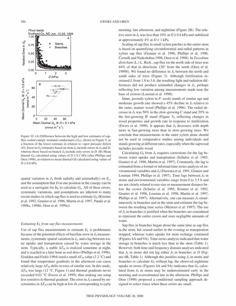
Figure 10. (A) Difference between the high and low estimates of sap-flux-scaled canopy stomatal conductance (GS), shown in Figure 9, asa fraction of the lower estimate in relation to vapor pressure deficit(D). Error in GS estimates based on stem JS include errors in JS and D,whereas those based on branch JS include only errors in D. (B) Meandiurnal GS calculated using values of D ≥ 0.1 kPa (after Phillips andOren 1998), in relation to mean diurnal GS calculated using values ofD ≥ 0.6 kPa.

Estimating δW

Estimates of GS suffer not only from errors in estimating JS

(Figure 2B) and stem recharge (Figures 4A and 9A) but alsofrom errors in estimating the driving force for transpiration.Errors in the driving force may originate from measurementerrors of TL, TA, and RH, and from systematic variation alongthe canopy profile. Castellvi et al. (1996) found that RH esti-mated from mean daily dewpoint temperature, mean daily TA,and diurnal pattern of TA had an error of up to 9% comparedwith RH measured with the more accurate but less automateddewpoint hygrometer. Given patterns in TA and RH found inthis study (Figure 5A), the largest measurement errors in TA

translated to a maximum error in D of 3.9%. However, errorsin measurement of RH may cause large errors in D, exceeding10% when D < 0.6 kPa (Figures 5B, 6A and 6B).

In well-coupled stands when wind speed is sufficiently high(Martin et al. 1999), TL is often assumed to be similar to TA,justifying the use of D as a proxy for δW for calculating GS

(Köstner et al. 1992, Granier et al. 1996, Martin et al. 1997,Oren et al. 1998). We did not evaluate the effect of errors in es-timates of emissivity on the measurement of TL with an infra-red thermometer, but these errors can be large (Gay andKnoerr 1975). Provided that the emissivity used in this study iscorrect, TL was indistinguishable from TA (Figure 8A) justify-ing the use of D as a surrogate for δW (Figure 8B).

In most studies, D is calculated for one position within orabove the canopy (Köstner et al. 1992, Granier et al. 1996,Martin et al. 1997, Oren et al. 1998, Pataki et al. 1998a,1998b). This assumes that vertical gradients in TA and RH aresmall and their effects on GS estimates are negligible. Temp-erature gradients may be as high as 5 °C in shrub canopiesand 17 °C in pasture (Tappeiner and Cernusca 1996), both ofwhich are less aerodynamically turbulent than many conifer-ous and some broadleaf forests. In coniferous and other forestswith high canopy roughness, the air within the canopy is con-sidered well mixed with the air above the canopy, at least dur-ing daytime when the mechanical production of turbulentkinetic energy is high (Oke 1995). This should result in a rela-tively weak gradient of D within the canopy.

In forests where aerodynamic turbulence is low, the simpli-fication of Equation 2 cannot be used and a radiative termmust be added (Monteith and Unsworth 1990). Furthermore,multiple measurements of D would be needed in a vertical ar-ray to measure the vertical gradients of D that result in forestsof low aerodynamic conductance. Aerodynamic conductancein all stands at our study site was estimated to be 33-foldhigher than total canopy conductance (Ewers et al. 1999). Thisdifference is reflected in the similarity observed between D inan opening and D inside stands differing twofold in L and theabsence of a vertical gradient in D (Figure 7). This is similar tofindings in a Pinus sylvestris L. stand (L = 2.8, height = 12 m),where D changed vertically only at an aerodynamic conduc-tance of 0.001 kPa m–1 (Joss and Graber 1996). At our studysite, a gradient in D below the canopy was found only underconditions caused by irrigation or a nearby large opening (Fig-ures 7E and 7F). Thus, the assumption that a single RH–TA sen-

sor is sufficient to provide an estimate of D throughout thecanopy is valid for P. taeda and similar forests.

Conditional sampling approaches for calculating GS

Analysis of measurement errors indicated that, to estimate GS

within 10% of error-free values, data should be selected forD ≥ 0.6 to 1.0 kPa (Figure 10A). Phillips and Oren (1998) em-ployed a statistically based conditional sampling approach toreduce the errors in estimating GS. This statistical approach re-moved from the analysis rain days, all values of GS corre-sponding to times in which D < 0.1 kPa, and all days with lessthan 12 GS values after applying the second criterion. Based onthese selection criteria, an acceptable agreement was obtainedbetween the mean of the remaining half-hour data and a meandaily GS (<GS>) computed directly from the daily sum of JS

and the daily mean daytime D. Phillips and Oren (1998) antici-pated that the mean of diurnal GS values will be lower than<GS> because, unlike <GS>, GS does not incorporate the waterthat is transpired during the day but taken up during the night.Based on the criteria for conditional sampling obtained here(i.e., D ≥ 0.6 kPa), mean diurnal GS values were generallygreater than <GS>, and there was no difference between use ofD ≥ 0.6 kPa or D ≥ 1.0 kPa as a filter (P > 0.5). As a result, theGS calculated as recommended here was higher than that cal-culated as suggested by Phillips and Oren (1998; Figure 10B);however, the means estimated by two approaches convergedfor days of high conductance.

The conditional sampling method proposed here does notexclude rain days and is not limited by a requisite minimumnumber of points for estimating GS, unlike the statisticallybased approach proposed in Phillips and Oren (1998). How-ever, the statistically based approach permits use of data whenD is low (i.e., D ≥ 0.1 kPa). Environmental conditions maydictate which approach is used to calculate GS (e.g., the statis-tically based approach may be more suitable in moist environ-ments where a large proportion of the data would be excludedat D < 0.6 kPa). Nevertheless, the approach developed herelimits the data to the range in which estimates of GS have alower uncertainty (Figure 10A).

Acknowledgments

This research was funded by USDA Forest Service Grant andWestvaco Co., the National Science Foundation through GrantBIR-9512333, and the US Department of Energy through the South-east Regional Center at the University of Alabama (CooperativeAgreement No. DE-FC03-90ER61010). The authors are grateful toPeter Anderson and Greg Burkeland for technical assistance. Thiswork contributes to the Global Change and Terrestrial Ecosystem(GCTE) core project of the International Geosphere-Biosphere Pro-gram (IGBP).

References

Albaugh, T.J., H.L. Allen, P.M. Dougherty, L.W. Kress and J.S.King. 1998. Leaf area and above-and belowground growth re-sponses of loblolly pine to nutrient and water additions. For. Sci.44:317–328.



Arneth, A., F.M. Kelliher, G. Bauer, D.Y. Hollinger, J.N. Byers, J.E.Hunt, T.M. McSeveny, W. Ziegler, N.N. Vygodskaya, I.Milukova, A. Sogachov, A. Varlagin and E.-D. Schulze. 1996. En-vironmental regulation of xylem sap flow and total conductance ofLarix gmelinii trees in eastern Siberia. Tree Physiol. 16:247–255.

Baldocchi, D. and T. Meyers. 1998. On using eco-physiological,micrometerological and biogeochemical theory to evaluate carbondioxide, water vapor and trace gas fluxes over vegetation: a per-spective. Agric. For. Meteorol. 90:1–15.

Brocklebank, J.C. and D.A. Dickey. 1986. SAS system for forecast-ing time series. SAS Institute Inc., Cary, NC, 240 p.

Castellvi, F., P.J. Perez, J.M. Villar and J.I. Rosell. 1996. Analysis ofmethods for estimating vapor pressure deficits and relative humid-ity. Agric. For. Meteorol. 82:29–45.

Cienciala, E., A. Lindroth, J. Èermák, J.-E. Hallgren and J. Kuèera.1994. The effects of water availability on transpiration, water po-tential and growth of Picea abies during a growing season. Trees6:121–127.

Èermák, J. and N. Nadezhdina. 1998. Sapwood as the scaling parame-ter—defining according to xylem water content or radial pattern ofsap flow. Ann. Sci. For. 55: 409–521.

Diawara, A., D. Loustau and P. Berbigier. 1991. Comparison of twomethods for estimating the evaporation of a Pinus pinaster (Ait.)stand: sap flow and energy balance with sensible heat flux mea-surements by an eddy covariance method. Agric. For. Meteorol.54:49–66.

Ewers, B.E., R. Oren, T.J. Albaugh and P.M. Dougherty. 1999.Carry-over effects of long term water and nutrient supply on shortterm water use in Pinus taeda trees and stands. Ecol. Appl.9:513–525.

Gates, D.M. 1965. Radiant energy, its receipt and disposal. Metereol.Monogr. 6:1–26.

Gay, L.W. and K.R. Knoerr. 1975. The forest radiation budget. DukeUniversity School of Forestry and Environmental Studies. Dur-ham, NC, 165 p.

Goff, J.A. and S. Gratch. 1946. List 1947, Smithsonian Meteorologi-cal Tables. Trans. Am. Soc. Ventilation Engineer. 52:95.

Goulden, M.L. and C.B. Field. 1994. Three methods for monitoringthe gas exchange of individual tree canopies: ventilated-chamber,sap-flow and Penman-Monteith measurements on evergreen oaks.Funct. Ecol. 8:125–135.

Granier, A. 1987. Evaluation of transpiration in a Douglas-fir stand bymeans of sap flow measurements. Tree Physiol. 3:309–320.

Granier, A. and D. Loustau. 1994. Measuring and modeling the tran-spiration of a maritime pine canopy from sap-flow data. Agric. For.Meteorol. 71:61–81.

Granier, A., P. Biron, B. Köstner, L.W. Gay and G. Najjar. 1996.Comparisons of xylem sap flow and water vapour flux at the standlevel and derivation of canopy conductance for Scots pine. Theor.Appl. Climat. 53:115–122.

Herbst, M. 1995. Stomatal behavior in a beech canopy: an analysis ofBowen ratio measurements compared with porometer data. PlantCell Environ. 18:1010–1018.

Hinckley, T.M., D.G. Sprugel, J.R. Brooks, K.J. Brown, T.A.Martin,D.A. Roberts, W. Schaap and D. Wang. 1998. Scaling and integra-tion in trees. In Ecological Scale: Theory and Application. Eds.D.L. Peterson and V.T. Parker. Columbia University Press, NewYork, pp 309–337.

Jarvis, P.G. 1995. Scaling processes and problems. Plant Cell Envi-ron. 18:1079–1089.

Jarvis, P.G. and K.G. McNaughton. 1986. Stomatal control of transpi-ration: scaling up from leaf to region. Adv. Ecol. Res. 15:1–49.

Joss, U. and W.K. Graber. 1996. Profiles and simulated exchange ofH2O, O3, NO2 between the atmosphere and the HartX Scots pineplantation. Theor. Appl. Clim. 53:157–172.

Köstner, B.M., E.-D. Schulze, F.M. Kelliher, D.Y. Hollinger, J.N.Byers, J.E. Hunt, T.M. McSeveny, R. Meserth and P.L. Weir.1992. Transpiration and canopy conductance in a pristinebroad-leaved forest of Nothofagus: an analysis of xylem sap flowand eddy correlation measurements. Oecologia 91:350–359.

Köstner, B., A. Granier and J. Èermák. 1998. Sapflow measurementsin forest stands: methods and uncertainties. Ann. Sci. For. 55:13–27.

Loustau, D., P. Berbigier, P. Roumagnac, C. Arruda-Pacheco, J.S.David, M.I. Ferreira, J.S. Pereira and R. Tavares. 1996. Transpira-tion of a 64-year-old maritime pine stand in Portugal. 1. Seasonalcourse of water flux through maritime pine. Oecologia 91:350–359.

Loustau, D., J.-C. Domec and B. Alexandre. 1998. Interpreting thevariations in xylem sap flux density within the trunk of maritimepine (Pinus pinaster Ait.): application of a model for calculatingwater flows at tree and stand levels. Ann. Sci. For. 55:29–46.

Leverenz, J., J.D. Deans, E.D. Ford, P.G. Jarvis, R. Milne andD. Whitehead. 1982. Systematic spatial variation of stomatal con-ductance in a Sitka spruce plantation. J. Appl. Ecol. 19:835–851.

Martin, T.A., K.J. Brown, J. Èermák, R. Ceulemans, J. Kuèera, F.C.Meinzer, J.S. Rombold, D.G. Sprugel and T.M. Hinckley. 1997.Crown conductance and tree and stand transpiration in a secondgrowth Abies amibilis forest. Can. J. For. Res. 27:797–808.

Martin, T.A., T.M. Hinckley, F.C. Meinzer and D.G. Sprugel. 1999.Boundary layer conductance, leaf temperature and transpiration ofAbies amabilis branches. Tree Physiol. 19:435–443.

Megraw, R.A. 1985. Wood quality factors in loblolly pine. Tappi, At-lanta, GA, 88 p.

Meinzer, F.C., T.M. Hinckley and R. Ceulemans. 1997. Apparent re-sponses of stomata to transpiration and humidity in a hybrid poplarcanopy. Plant Cell Environ. 16:429–426.

Murthy, R., P.M. Dougherty, S.J. Zarnoch and H.L. Allen. 1996. Ef-fects of carbon dioxide, fertilization, and irrigation onphotosynthetic capacity of loblolly pine trees. Tree Physiol.16:537–546.

Monteith, J.L. and M.H. Unsworth. 1990. Principles of environmen-tal physics. Edward Arnold, London, 291 p.

Oke, T.R. 1995. Boundary layer climates. Routledge, London, 435 p.Oren, R., N. Phillips, G. Katul, B.E. Ewers and D.E. Pataki. 1998.

Scaling xylem sap flux and soil water balance and calculating vari-ance: a method for partitioning water flux in forests. Ann. Sci. For.55:191–216.

Oren, R., J.S. Sperry, G.G. Katul, D.E. Pataki, B.E. Ewers, N. Phillipsand K.V.R. Schäfer. 1999a. Survey and synthesis of intra- andinterspecific variation in stomatal sensitivity to vapour pressuredeficit. Plant Cell Environ. 22:1515–1526.

Oren, R., N. Phillips, B.E. Ewers, D.E. Pataki and J.P. Megonigal.1999b. Responses of sap flux-scaled transpiration to light, vaporpressure deficit, and leaf area reduction in a flooded Taxodiumdistichum L. forest. Tree Physiol.19:337–347.

Pataki, D.E., R. Oren and D.T. Tissue. 1998a. Elevated carbon diox-ide does not affect average canopy stomatal conductance of Pinustaeda L. Oecologia 117:47–52.

Pataki, D.E., R. Oren, G. Katul and J. Sigmon. 1998b. Canopy con-ductance of Pinus taeda, Liquidambar styriciflua and Quercusphellos under varying atmospheric and soil water conditions. TreePhysiol. 18:307–315.

588 EWERS AND OREN


Pearcy, R.W., E.-D. Schulze and R. Zimmerman. 1989. Measurementof transpiration and leaf conductance. In Plant Physiological Ecol-ogy. Eds. R.W. Pearcy, J. Ehleringer, H.A. Mooney and P.W.Rundel. Chapman and Hall, London, pp 137–160.

Phillips, N. and R. Oren. 1998. A comparison of daily representationsof canopy conductance based on two conditional time-averagingmethods and the dependence of daily conductance on environmen-tal factors. Ann. Sci. For. 55:191–216.

Phillips, N., R. Oren and R. Zimmerman. 1996. Radial patterns of xy-lem sap flow in non-, diffuse-, and ring-porous tree species, PlantCell Environ. 19:983–990.

Phillips, N., A. Nagchaudhuri, R. Oren and G. Katul. 1997. Time con-stant for water uptake in loblolly estimated form times series ofstem sapflow and evaporative demand. Trees 11:412–419.

Schulze, E.-D., J. Èermák, R. Matyssek, M. Penka, R. Zimmerman,F. Vasicek, W. Gries and J. Kuèera. 1985. Canopy transpirationand water fluxes in the xylem of the trunk of Larix and Piceatrees—a comparison of xylem flow, porometer and cuvette mea-surements. Oecologia 66:475–483.

Sellers, P.J, R.E. Dickinson, D.A. Randall, et al. 1997. Modeling theexchange of energy, water, and carbon between continents and theatmosphere. Science 275:502–509.

Tappeiner, U. and A. Cernusca. 1996. Microclimate and fluxes of wa-ter vapour, sensible heat and carbon dioxide in structurally differ-ing subalpine plant communities in the central Causcasus. PlantCell Environ. 19:403–417.



analyses of assumptions and errors in the calculation of ... pdf/ewers...represents sap flux in the...

Documents