analysis and classification of electroencephalography signals · 2019-01-02 · analysis and...

ANALYSIS AND CLASSIFICATION OF

ELECTROENCEPHALOGRAPHY

SIGNALS

A THESIS SUBMITTED IN PARTIAL REQUIREMENTS FOR THE DEGREE OF

BACHELOR OF TECHNOLOGY

IN

ELECTRONICS & COMMUNICATION ENGINEERING

BY

AMIT KUMAR VERMA

ROLL NO. 10609021

&

ANOOP KUMAR MANGARAJ

ROLL NO. 10609011

UNDER THE GUIDANCE OF

PROF. SAMIT ARI

DEPARTMENT OF ELECTRONICS AND COMMUNICATION ENGINEERING

NATIONAL INSTITUTE OF TECHNOLOGY, ROURKELA

National Institute of Technology,

Rourkela

CERTIFICATE

This is to certify that the thesis entitled, “Analysis and Classification of

Electroencephalography signals” submitted by Amit Kumar Verma and Anoop

Kumar Mangaraj in partial fulfillment of requirements for the award of Bachelors

in Technology degree in Electronics and Communication Engineering, Department

of Electronics and Communication Engineering at National Institute of

Technology, Rourkela (Deemed University) is an authentic work carried out by

them under my supervision and guidance.

To the best of my knowledge, the matter embodied in the thesis has not

been submitted to any university /institute for award of any degree or diploma.

Date: 10th May, 2010 Prof. Samit Ari

Dept. of Electronics & Communication Engg

. National Institute of Technology

. Rourkela- 769008

ACKNOWLEGDEMENT

We take this opportunity to thank all the individuals whose guidance, help and timely

support made us to complete the project within the stipulated time. Unfortunately it isn‟t possible

to express our thanks to all of them in a single page of acknowledgement.

First and foremost we would like to express our sincere gratitude to our project

supervisor Prof. Samit Ari for his invaluable support, motivation, guidance and constant

encouragement which made this project a rich and insightful experience. His timely inputs,

valuable feedbacks and constructive criticism in many stages of this work were instrumental in

understanding and execution of this project.

We are also grateful to Prof. S.K. Patra (Head of the Department), Department of

Electronics and Communication engineering for assigning us this interesting project and

providing us with various facilities of the department. His valuable suggestions and inspiring

guidance were extremely helpful.

An assemblage of this nature could never have been attempted without reference to and

inspiration from the works of others whose details are mentioned in reference section. We

acknowledge our indebtedness to all of them.

We would also like to thank all professors and lecturers, and members of the department

for their generous help in various ways for the completion of this thesis. We also extend our

thanks to our dear friends for their support and cooperation.

Date: 10th May 2009

Place: NIT Rourkela

Amit Kumar Verma Anoop Kumar Mangaraj

Dept. of ECE Engineering Dept. of ECE Engineering

National Institute of Technology National Institute of Technology

Rourkela – 769008 Rourkela – 769008

Contents

Abstract……………………………………………..……………………………...i

List of figures………………………………………..…………………………….ii

List of tables…………………………………………………………………..…..iv

1. Introduction………………………………………..…………………………...1

1.1 What are EEG signals?..........................................................................................2

1.2 EEG generation………………………………………………………..………..2

1.3 EEG recording………………………………….………………………..……...3

1.4 Brain rhythms………………………………...…………………………...…….4

1.5 Why do we use EEG signals?..................................................................................5

1.6 Objective…………………………………………………………………..…...6

1.7 Data selection………………………………………………………………..….7

1.8 Raw EEG signal………………………………….………………………….….8

2. Classification of EEG signal……………………………………………….…10

2.1 Wavelet transform…………………………………………………………..….11

2.1.1 Continuous wavelet transform…………………………………………..…12

2.1.2 Discrete wavelet transform……………………………………………..…12

2.1.3 Wavelet families………………………………………………………....14

2.2 Feature extraction using Discrete wavelet transform…..…………………………..15

2.3 Feature Extraction using Autoregressive Coefficients……………...……………….18

2.4 feature vector………………………………………………….……………….21

2.5 Artificial neural network.......................................................................................23

2.6 Learning Process……………………………………………………………….25

2.7 MLPNN and back propagation algorithm……………..…………………………..26

2.8 Committee neural network……………………………………….……………...27

2.9 Classification using Committee neural network…………..………………………..28

3. Dimensionality reduction using F-ratio……………………………………...32

3.1 F-ratio………………………………………………………………………...33

3.2 Dimension reduction using F-ratio………………….……………………………34

3.3 F-ratio of extracted features……………………….…………………………….35

4. Conclusion & Future Work ………………………………………………….38

References………………………………………………………………………...40

ABSTRACT

EEG signal processing is one of the hottest areas of research in digital signal processing

applications and biomedical research. Analysis of EEG signals provides a crucial tool for

diagnosis of neurobiological diseases. The problem of EEG signal classification into healthy and

pathological cases is primarily a pattern recognition problem using extracted features. Many

methods of feature extraction have been applied to extract the relevant characteristics from a

given EEG data. The EEG data was collected from a publicly available source. Three types of

cases were classified viz. signals recorded from healthy volunteers having their eyes open,

epilepsy patients in the epileptogenic zone during a seizure-free interval, and epilepsy patients

during epileptic seizures. The feature extraction was done by computing the discrete wavelet

transform and spectral analysis using AR model. The wavelet transform coefficients compress

the number of data points into few features. Various statistics were used to further reduce the

dimensionality. The AR coefficients obtained from burg auto-regressive method provide

important features of the EEG signals. Classification of the EEG data using committee neural

network provides robust and improved performance over individual members of the committee.

F-ratio based dimension reduction technique was used to reduce the number of features without

affecting the accuracy much.

i

LIST OF FIGURES

Figure 1.1: Schematic view of the scalp……………………………..…………….…......2

Figure 1.2: Structure of a neuron........................................................................................3

Figure 1.3: Conventional 10-20 electrode placement scheme............................................4

Figure 1.4: Block diagram of EEG signal processing........................................................7

Figure 1.5(a) EEG segment of class A…………………………………………….……..8

(b) EEG segment of class D................................................................................9

(c) EEG segment of class E................................................................................9

Figure 2.1: Representation of a wave and wavelet...........................................................11

Figure 2.2: DWT computation using filter banks.............................................................13

Figure 2.3: Wavelet families…………………………………………..…………….......15

Figure 2.4: (a)Wavelet coefficients of class A……………………………………….…17

(b)Wavelet coefficients of class D.................................................................17

(c)Wavelet coefficients of class E……………………………………….…18

Figure 2.5: (a) Power spectral density of class A using AR model.................................20

(b) Power spectral density of class D using AR model................................20

(c) Power spectral density of class E using AR model.................................21

ii

Figure 2.6: (a) Feature vector of class A..........................................................................21

(b)Feature vector of class D..........................................................................22

(c)Feature vector of class E...........................................................................22

Figure 2.7: Model of a neuron..........................................................................................23

Figure 2.8: Structure of a neural network.........................................................................24

Figure 2.9: Committee neural network............................................................................28

Figure 3.1: Diagram for multi-cluster data.......................................................................33

iii

LIST OF TABLES

Table 2.1: Statistics of wavelet coefficients......................................................................16

Table 2.2: Confusion matrix of neural network 1.............................................................29



Table 2.5: Statistical parameters of neural network 1.......................................................30



Table 2.8: Statistical parameters of Committee neural network.......................................31

Table 2.9: Accuracy of Committee neural network………………………..……………31

Table 3.1: F-ratio of the extracted features.......................................................................35

Table 3.2: Reduction of features.......................................................................................36

iv

1

Chapter 1

Introduction

2

1.1 What are EEG Signals?

Electroencephalography (EEG) is the recording of spontaneous electrical activity of the brain

which is obtained by firing of neurons within the brain. EEG signals are recorded in a short time,

normally for 20-40 minutes. We get the recordings by placing the electrodes at various positions

on the scalp. Figure.1 shows the schematic view of the scalp and dots represent the placing of the

multiple electrodes on the scalp. It is believed that the EEG signals not only represents the brain

signal but represents the status of the whole body. The diagnostic application in case of epilepsy

gives us the prime motivation to apply the Digital Signal Processing techniques to the EEG

signals.

Figure 1.1: Schematic view of the scalp [20]

1.2 EEG generation

An EEG signal is generated due to the currents that flow between the brain cells in the cerebral

cortex region of the brain. When the neurons are activated, current flows between dendrites due

to their synaptic excitations. This current generates a magnetic field and a secondary electric

3

field. The magnetic field is measurable by electromyogram (EMG) machines and the electric

field is measured by EEG systems over the scalp [1].

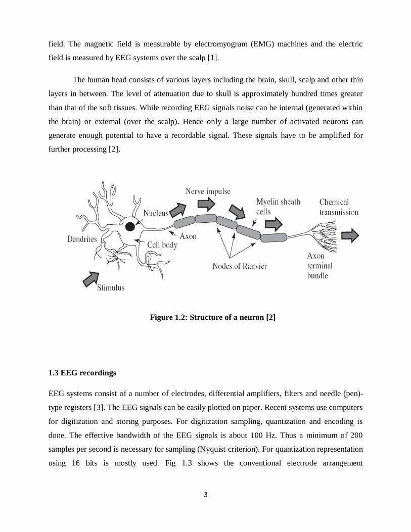
The human head consists of various layers including the brain, skull, scalp and other thin

layers in between. The level of attenuation due to skull is approximately hundred times greater

than that of the soft tissues. While recording EEG signals noise can be internal (generated within

the brain) or external (over the scalp). Hence only a large number of activated neurons can

generate enough potential to have a recordable signal. These signals have to be amplified for

further processing [2].

Figure 1.2: Structure of a neuron [2]

1.3 EEG recordings

EEG systems consist of a number of electrodes, differential amplifiers, filters and needle (pen)-

type registers [3]. The EEG signals can be easily plotted on paper. Recent systems use computers

for digitization and storing purposes. For digitization sampling, quantization and encoding is

done. The effective bandwidth of the EEG signals is about 100 Hz. Thus a minimum of 200

samples per second is necessary for sampling (Nyquist criterion). For quantization representation

using 16 bits is mostly used. Fig 1.3 shows the conventional electrode arrangement

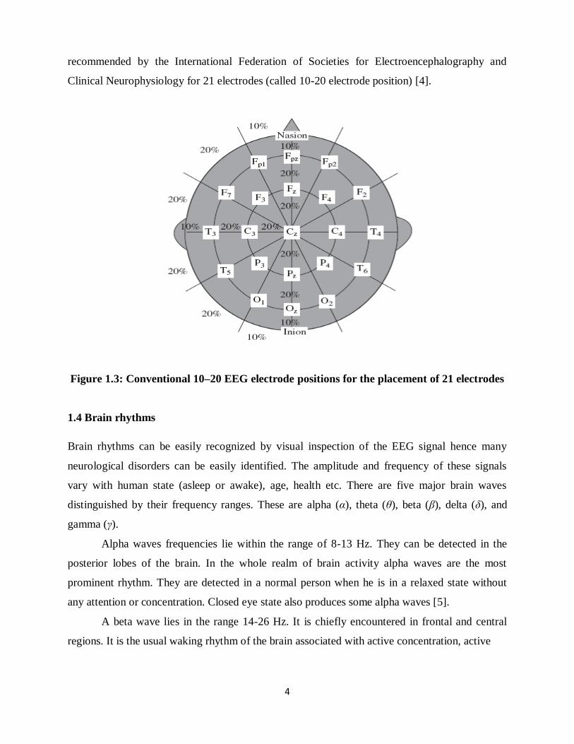
4

recommended by the International Federation of Societies for Electroencephalography and

Clinical Neurophysiology for 21 electrodes (called 10-20 electrode position) [4].

Figure 1.3: Conventional 10–20 EEG electrode positions for the placement of 21 electrodes

1.4 Brain rhythms

Brain rhythms can be easily recognized by visual inspection of the EEG signal hence many

neurological disorders can be easily identified. The amplitude and frequency of these signals

vary with human state (asleep or awake), age, health etc. There are five major brain waves

distinguished by their frequency ranges. These are alpha (α), theta (θ), beta (β), delta (δ), and

gamma (γ).

Alpha waves frequencies lie within the range of 8-13 Hz. They can be detected in the

posterior lobes of the brain. In the whole realm of brain activity alpha waves are the most

prominent rhythm. They are detected in a normal person when he is in a relaxed state without

any attention or concentration. Closed eye state also produces some alpha waves [5].

A beta wave lies in the range 14-26 Hz. It is chiefly encountered in frontal and central

regions. It is the usual waking rhythm of the brain associated with active concentration, active

5

thinking, problem solving, focussing on things. When a person is in a panic state a high level

beta wave is generated [6].

Theta waves lie within the range 4-7.5 Hz. It is assumed that it has origins in the thalamic

region. When a person is slipping into a drowsy state from conscious state theta waves are

observed. They play a crucial role in infants and young children. Creative thinking, deep

meditation, access to unconscious material is associated with theta waves [7].

Delta waves are within the range 0.5-4 Hz. They are found frontally in adults and

posteriorily in children. They are associated with deep sleep and may be present in waking state.

Gamma waves are also called fast beta waves and they have frequencies above 30 Hz.

The amplitude of these waves is very low and they have rare occurrence. They are associated

with certain cognitive and motor functions. Detection of these rhythms can be used to confirm

certain neurological diseases. It is also a good indicator of event related synchronisation (ERS)

of the brain [8].

1.5 Why do we use EEG signals?

There are various advantages of EEG signals some of them can be states as follows:

Temporal resolution of the EEG signal is high.

EEG measures the electrical activity directly.

EEG is a non-invasive procedure.

It has the ability to analyze the brain activity; it unfolds in real time at level of

milliseconds, i.e. thousands of a second.

It is very hard to find the source of electrical activity where the electrical activity is coming

from. This is the major disadvantages of EEG signals. By placing the multiple electrodes on the

scalp we can get some information where the ERP is strongest.

6

EEG signals are used for various tasks. We can divide the uses of EEG as clinical uses and

research uses [21]:

Clinical uses:

EEG signals are used in the diagnosis of several neurological diseases.

EEG signals are used to characterize the seizures for the purpose of treatment.

EEG signals are used to monitor the depth of anesthesia.

EEG signals are used to determine the wean-epileptic medication.

Research uses:

EEG signals are used in neuroscience.

EEG signals are used in cognitive science.

EEG signals can be used for the psychophysiological research.

EEG signals can be used for the study of the responses to auditory stimuli.

1.6 Objective

Our objective is to analyze the EEG signals and classify the EEG data into different classes. Our

main target is to improve the accuracy of EEG signals. In our project we have also applied

optimization techniques to reduce the computation complexity of the network without affecting

the accuracy of the classification.

Figure. 4 shows the block diagram for the EEG signal processing. For the classification

purpose we have taken the raw EEG signals available at [9]. From the five data sets available we

have selected 3 sets (set A, set D, set E). In set A EEG signals were recorded from healthy

volunteers. In set D recordings were taken from within epiletogenic zone but during seizure free

interval while set E contained only seizure activity. For each of these data we extracted the

features using discrete wavelet transform and Auto-Regressive coefficients method. After feature

extraction the different data sets were classified using committee neural network trained with

back propagation algorithm. To reduce the dimensionality of the features we have used Fisher‟s

ratio based optimization technique.

7

Figure 1.4: Block diagram of EEG signal classification

In chapter 2 our proposed technique for the classification purpose is discussed, then in the

chapter 3 F-ratio based technique to reduce computational complexity. In chapter 4 we conclude

our thesis along with future work.

1.7 Data Selection

The EEG data used in this study was obtained from the database available with the Bonn

University. This data is publicly available at [9]. The complete dataset consists of five classes (A,

B, C, D, E) each of which contains 100 single channel EEG segments of 23.6s duration. Each

segment was selected and cut out from continuous multichannel EEG recordings after visual

inspection for artifacts e.g. due to eye movement or muscle activity.

Sets A and B consisted of signals taken from surface EEG recordings that were carried

out on five healthy volunteers using a standardized electrode placement scheme (International

8

10–20 system). Volunteers were relaxed in an awake state with eyes open (A) and eyes closed

(B), respectively. Sets C–E originated from the EEG archive of presurgical diagnosis. EEGs

from five patients were selected, all of whom had achieved complete seizure control after

resection of one of the hippocampal formations, which was therefore correctly diagnosed to be

the epileptogenic zone. Signals in set D were recorded from within the epileptogenic zone, and

those in set C from the hippocampal formation of the opposite hemisphere of the brain. While

sets C and D contained only activity measured during seizure-free intervals, set E only contained

seizure activity.

Using an average common reference, all EEG signals were recorded with the same 128-

channel amplifier system. The data were digitized at 173.61 samples per second using 12 bit

analog-to-digital converter. The settings of the band pass filter were 0.53–40 Hz (12 dB/oct.)

[10]. In the present study sets A, D, E was used.

1.8 Raw EEG signal

From the data available at [9], a rectangular window of length 256 discrete data was selected to

form a single EEG segment. The plot of segment of the three classes (A, D, E) is shown below

(a)

9

(b)

(c)

Figure 1.5 (a) EEG segment of class A (b) EEG segment of class D (c) EEG segment

of class E

10

Chapter 2

Classification of EEG

Signal

11

2.1 Wavelet Transform

The transform of a signal is just another way of representing a signal as it doesn‟t change any

information content of a signal. Although short time Fourier transform (STFT) can be used to

analyze non-stationary signals, it has a constant resolution at all frequencies. The wavelet

transform gives a time-frequency representation and in this transform different frequencies are

analyzed with different resolutions.

Wavelet transform uses wavelets of finite energy. Wavelets are localized waves which

are suited to analyze transients since their energy is concentrated in time and space [11].

(a) (b)

Figure 2.1 Representation of (a ) wave (b) wavelet

The wavelet transform gives us multi-resolution description of a signal. It addresses the

problems of non-stationary signals and hence is particularly suited for feature extraction of EEG

signals [12]. At high frequencies it provides a good time resolution and for low frequencies it

provides better frequency resolution, this is because the transform is computed using a mother

wavelet and different basis functions which are generated from the mother wavelet through

scaling and translation operations. Hence it has a varying window size which is broad at low

frequencies and narrow at high frequencies, thus providing optimal resolution at all frequencies.

12

2.1.1 Continuous wavelet transform

The continuous wavelet transform is defined as

𝑋𝑊𝑇(𝜏, 𝑠) =1

| 𝑠 | 𝑥 𝑡 . 𝜓(

𝑡 − 𝜏

𝑠) 𝑑𝑡

Where x(t) is the signal to be analyzed , ψ(t) is the mother wavelet or the basis function τ

is the translation parameter and s is the scale parameter.

The Continuous wavelet transform performs the convolution operation of the basis

function and the signal. The mother wavelet is chosen depending upon the characteristics

associated with the signal. The translation parameter τ relates to the time information present in

the signal and it is used to shift the location of the wavelet function in the signal. The scale

parameter s correspond to the frequency information is defined as the inverse of frequency.

Scaling expands or contracts a signal, hence large scales expand the signal and give the hidden

local information while small scales contract a signal and provide global information [11].

2.1.2 Discrete wavelet transform

The computation of CWT consumes a lot of time and resources and results in large amount of

data, hence Discrete wavelet transform, which is based on sub-band coding is used as it gives a

fast computation of wavelet transform. In DWT the time-scale representation of the signal can be

achieved using digital filtering techniques. The approach for the multi-resolution decomposition

of a signal x(n) is shown in Fig. 2.2. The DWT is computed by successive low pass and high pass

filtering of the signal x(n). Each step consists of two digital filters and two downsamplers by 2.

The high pass filter g[] is the discrete mother wavelet and the low pass filter h[.] is its mirror

version. At each level the downsampled outputs of the high pass filter produce the detail

coefficients and that of low pass filter gives the approximation coefficients. The approximation

coefficients are further decomposed and the procedure is continued as shown [13-14].

13

Figure: 2.2 Discrete wavelet transform block diagram [15]

The standard quadrature filter condition is

𝐻 𝑧 𝐻 𝑧−1 + 𝐻 −𝑧 𝐻 −𝑧−1 = 1

where H(z) is the Z-transform the low pass filter h. this filter can be used to specify all wavelet

transforms.

The complementary high pass filter is defined as

𝐺 𝑧 = 𝑧𝐻(−𝑧−1)

Now the sequence of filters can be obtained as

𝐻𝑘+1 𝑧 = 𝐻 𝑧2𝑘 𝐻𝑘 𝑧 ,

𝐺𝑘+1 = 𝐺 𝑧2𝑘 𝐻𝑘 𝑧 , 𝑘 = 0,1 ……𝐾 − 1

with the initial condition H0(z) = 1. In time domain we have

𝑕𝑘+1 𝑛 = [𝑕]↑2𝑘 ∗ 𝑕𝑘(𝑛)

𝑔𝑘+1 𝑛 = [𝑔]↑2𝑘 ∗ 𝑕𝑘(𝑛)

The subscript [.]↑2k denotes upsampling by 2k. Here n is the discrete sampled time.

14

The normalized wavelet and scale basis function are defined as

𝜑𝑘 ,𝑙 = 2𝑘2𝑕𝑘(𝑛 − 2𝑘𝑙)

𝜓𝑘 ,𝑙 𝑛 = 2𝑘2𝑔𝑘(𝑛 − 2𝑘𝑙)

where the factor 2k/2

is the inner product normalization, k and l are the scale and translation

parameter respectively.

The DWT decomposition can be described as

𝑎 𝑘 𝑙 = 𝑥 𝑘 ∗ 𝜑𝑘 ,𝑙(𝑛)

𝑑 𝑘 𝑙 = 𝑥 𝑘 ∗ 𝜓𝑘 ,𝑙(𝑛)

where a(k)(l) and d(k)(l) are the approximation coefficients and the detail coefficients at

resolution k, respectively [13-16].

2.1.3 Wavelet families

There are a number of basic functions that can be used as the mother wavelet for Wavelet

transform. While choosing the mother wavelet the characteristics of the signal should be taken

into account since it produces the different wavelets through translation and dilation and hence

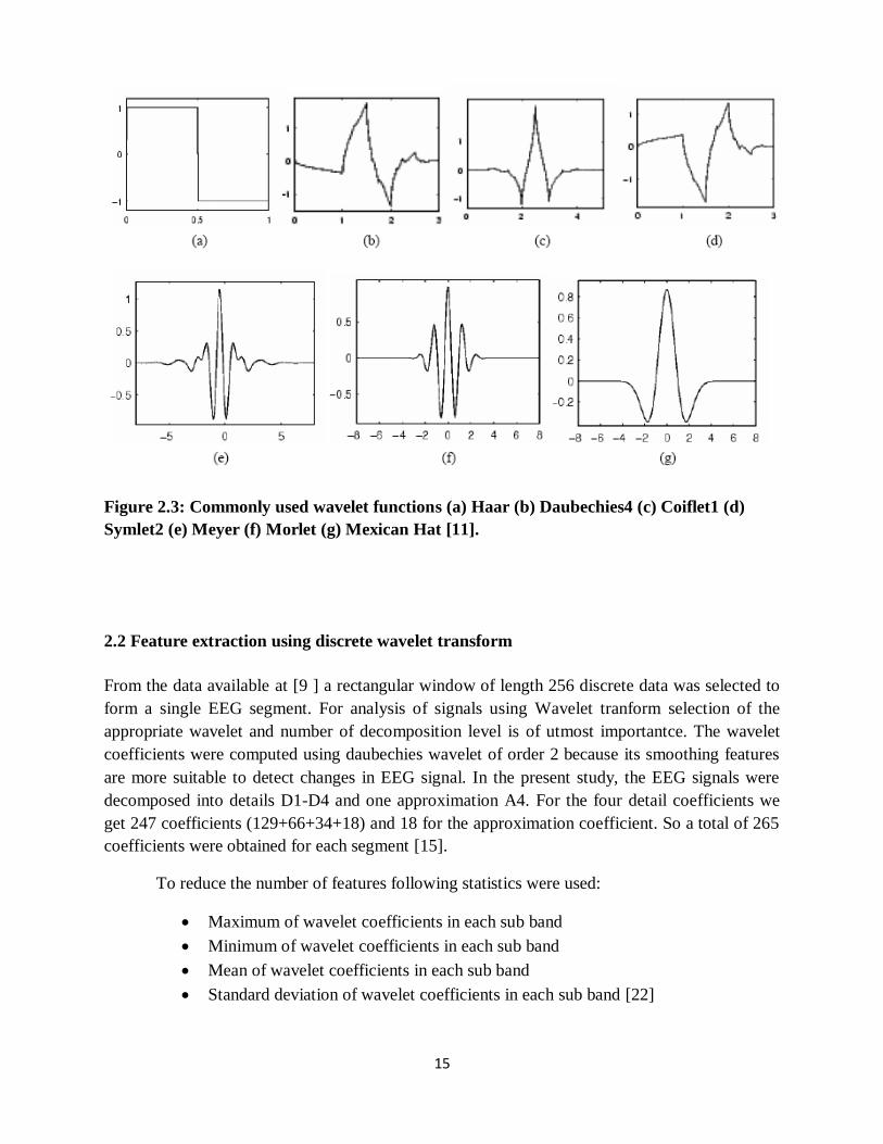
determines the characteristics of the resulting transform. Figure 2.3 illustrates the commonly

used wavelet functions. The wavelets are chosen on the basis of their shape and ability to analyze

the signal for a particular application.

15

Figure 2.3: Commonly used wavelet functions (a) Haar (b) Daubechies4 (c) Coiflet1 (d)

Symlet2 (e) Meyer (f) Morlet (g) Mexican Hat [11].

2.2 Feature extraction using discrete wavelet transform

From the data available at [9 ] a rectangular window of length 256 discrete data was selected to

form a single EEG segment. For analysis of signals using Wavelet tranform selection of the

appropriate wavelet and number of decomposition level is of utmost importantce. The wavelet

coefficients were computed using daubechies wavelet of order 2 because its smoothing features

are more suitable to detect changes in EEG signal. In the present study, the EEG signals were

decomposed into details D1-D4 and one approximation A4. For the four detail coefficients we

get 247 coefficients (129+66+34+18) and 18 for the approximation coefficient. So a total of 265

coefficients were obtained for each segment [15].

To reduce the number of features following statistics were used:

Maximum of wavelet coefficients in each sub band

Minimum of wavelet coefficients in each sub band

Mean of wavelet coefficients in each sub band

Standard deviation of wavelet coefficients in each sub band [22]

16

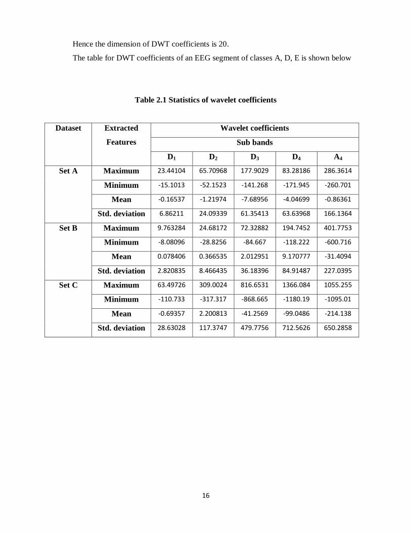
Hence the dimension of DWT coefficients is 20.

The table for DWT coefficients of an EEG segment of classes A, D, E is shown below

Table 2.1 Statistics of wavelet coefficients

Dataset Extracted

Features

Wavelet coefficients

Sub bands

D1 D2 D3 D4 A4

Set A Maximum 23.44104 65.70968 177.9029 83.28186 286.3614

Minimum -15.1013 -52.1523 -141.268 -171.945 -260.701

Mean -0.16537 -1.21974 -7.68956 -4.04699 -0.86361

Std. deviation 6.86211 24.09339 61.35413 63.63968 166.1364

Set B Maximum 9.763284 24.68172 72.32882 194.7452 401.7753

Minimum -8.08096 -28.8256 -84.667 -118.222 -600.716

Mean 0.078406 0.366535 2.012951 9.170777 -31.4094

Std. deviation 2.820835 8.466435 36.18396 84.91487 227.0395

Set C Maximum 63.49726 309.0024 816.6531 1366.084 1055.255

Minimum -110.733 -317.317 -868.665 -1180.19 -1095.01

Mean -0.69357 2.200813 -41.2569 -99.0486 -214.138

Std. deviation 28.63028 117.3747 479.7756 712.5626 650.2858

17

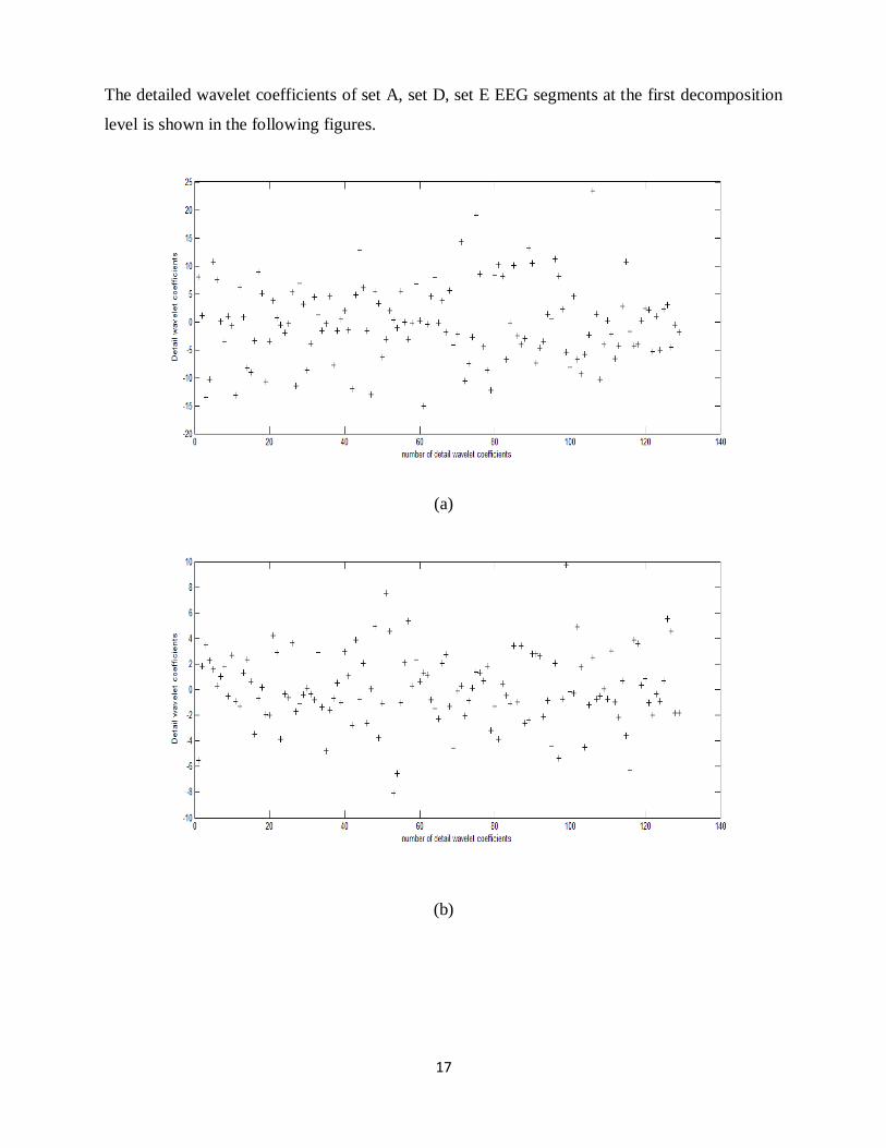
The detailed wavelet coefficients of set A, set D, set E EEG segments at the first decomposition

level is shown in the following figures.

(a)

(b)

18

(c)

Figure 2.4 (a), (b), (c) Plot for Discrete wavelet coefficients of class A, D and E respectively

2.3 Feature Extraction using Autoregressive Coefficients

The Autoregressive (AR) Power spectral density estimation of the EEG signals of set A, set B

and set C was computed. The Power spectral density is the distribution of power with respect to

the frequency. Power spectral density Rxx of the random stationary signal can be expressed by

polynomials A(z) and B(z) having roots that fall inside the unit circle in the z-plane [pr] as

shown in the given formula [23]

𝑅𝑥𝑥 𝑧 = 𝜎𝑤2 𝐵 𝑧 𝐵(𝑧−1)

𝐴 𝑧 𝐴(𝑧−1) , 𝑟1 < 𝑧 < 𝑟2

where σw is the variance of the white Gaussian noise w(n). Now the linear filter H(z) for

generating the random process x(n) from the white Gaussian noise w(n) can be written as

𝐻 𝑧 =𝐵(𝑧)

𝐴(𝑧)=

𝑏𝑘𝑧−𝑘𝑞𝑘=0

1+ 𝑎𝑘𝑧−𝑘𝑝𝑘=1

, 𝑧 > 𝑟1

19

Hence the output x(n) can be related to the input by using the following difference

equation:

𝑥 𝑛 + 𝑎𝑘𝑥 𝑛 − 𝑘 = 𝑏𝑘𝑤(𝑛 − 𝑘)

𝑞

𝑘=0

𝑝

𝑘=1

If b0 = 1, bk = 0, k > 0 then the linear filter H(z) can be written as 1/A(z). Now the

difference equation for the AR process can be reduced to

𝑥 𝑛 + 𝑎𝑘𝑥 𝑛 − 𝑘 = 𝑤(𝑛)

𝑝

𝑘=1

If ak = 0, k ≥ 1 then the linear filter H(z) = B(z) and the difference equation for the

moving average (MA) process can be written as follows:

𝑥 𝑛 = 𝑏𝑘𝑤(𝑛 − 𝑘)

𝑞

𝑘=0

In case of Autoregressive moving average (ARMA) process linear filter H(z) = B(z)/A(z)

has both finite poles and zeros in the z-plane [23].

Autoregressive coefficients are very important features as they represent the PSD of the

signal which is very common. Since the method characterizes the input data using an all-pole

model, the correct choice of the model order p is important. We cannot take the value of model

order too large or too small as it gives poor estimation of PSDs. We can model any stochastic

process using AR model.

There are various methods available for AR modeling such as moving average (MA)

model, autoregressive moving average (ARMA) model, Burg‟s algorithm [24]. ARMA method

of AR model is normally used to get good accuracy. Burg algorithm estimates the reflection

coefficient ak. we can use Burg method to fit a pth

order autoregressive (AR) model to the input

signal, x, by minimizing (least squares) the forward and backward prediction errors while

constraining the AR parameters to satisfy the Levinson-Durbin recursion [25]. The Burg method

is a recursive process.

In this paper we have followed the Burg‟s method to find the AR coefficients. The model

order is taken to be equal to 10. We have used the Burg algorithm to find the AR coefficients

using MATLAB.

20

AR coefficients and the Power spectral densitywere obtained by using MATLAB. Since the

model order is 10 we have 11 AR coefficients. The plot for the power spectral density is shown

in the following figures:

(a)

(b)

21

(c)

Figure 2.5 (a), (b), (c) Plot for power spectral density of class A, D and E

respectively

2.4 Feature Vector

The 20 discrete wavelet coefficients and 11 Auto-regressive coefficients were appended to form

feature vector of dimension 31. These feature coefficients are shown as follows:

(a)

22

(b)

(c)

Figure 2.6 (a), (b), (c) Feature vector of dimension 31 of class A, D and E

respectively

ut

23

s use 64 or 128 electrodes), we can get some idea of where the ERP components are strongest. This doesn't really

2.5 Artificial Neural Network

An artificial neural network can be defined as a machine that is modelled on a human brain. The

fundamental structural constituents of the brain are neurons which are also the basic information

processing units of an ANN. The neural network is formed by a massive interconnection of these

neurons. The network so formed has the capability of learning i.e acquiring knowledge from the

environment by performing computations. The synaptic weights which are the interneuron

connection strengths are used to store this acquired knowledge. In the learning process synaptic

weights can modified according to many algorithms to achieve the desired design objective. Fig

2.7 shows the model of a single neuron [18].

Figure 2.7: Model of a neuron

A typical neural network consists of the following layers

1. Input layer

2. Hidden layer

3. Output layer

The input layer consists of source nodes which supply the input vector (activation pattern) i.e the

input signals to the next layer.

24

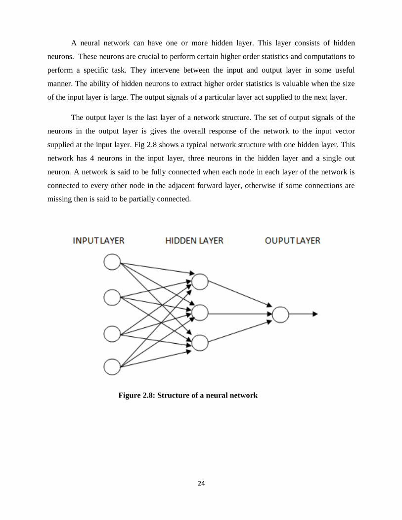
A neural network can have one or more hidden layer. This layer consists of hidden

neurons. These neurons are crucial to perform certain higher order statistics and computations to

perform a specific task. They intervene between the input and output layer in some useful

manner. The ability of hidden neurons to extract higher order statistics is valuable when the size

of the input layer is large. The output signals of a particular layer act supplied to the next layer.

The output layer is the last layer of a network structure. The set of output signals of the

neurons in the output layer is gives the overall response of the network to the input vector

supplied at the input layer. Fig 2.8 shows a typical network structure with one hidden layer. This

network has 4 neurons in the input layer, three neurons in the hidden layer and a single out

neuron. A network is said to be fully connected when each node in each layer of the network is

connected to every other node in the adjacent forward layer, otherwise if some connections are

missing then is said to be partially connected.

Figure 2.8: Structure of a neural network

25

2.6 Learning Process

Learning is a process in which the neural network undergoes changes in its free parameters when

it is stimulated by the environment. As a result of this learning it structure changes and it

responds in a new way to its environment. Gradually its performance improves through this

process. There are many types of learning rules, some of it are mentioned below [18].

Error- correction learning in which the error signal actuates a control mechanism so as

to make adjustments in to the synaptic weights. These changes make the output signal come

closer to the target value in a step by step manner. The error signal is the difference between the

desired output and the output from the network. The objective in this type of learning is to

minimize the cost function or the index of performance. The cost function is the instantaneous

value of the error energy.

Memory based learning- here all the past values of correctly classified input-output

examples are stored. When a new test pattern is applied to the network this learning algorithm

responds by retrieving and analyzing the training data in the local neighbourhood of the test

pattern. Nearest neighbour rule and K-nearest classifier are two popular algorithm in this type of

learning.

Hebbian learning-It is the oldest and most famous of all learning rules. It is based on

hebbian synapse which is defined as a synapse with time-dependent, highly local, and strongly

interactive mechanism to increase synaptic efficiency as a function of the correlation between

presynaptic and post synaptic activities. [Brown et al.,1990]. In other words if the neurons on

either side of a synapse are simultaneously activated then the strength of that synapse is

selectively increased and if activated asynchronously then the synapse is selectively weakened or

eliminated [Stent,1973; Changeux and Danchin 1976].

Competitive learning-As the name implies the output neurons of the network compete

among themselves to get become active. At a time only one neuron is activated. The set of

neurons are all same but for some randomly distributed synaptic weights, there is a mechanism in

place so that for the given input pattern only one neuron is fired i.e. the neuron that wins the

competition is called a winner-takes-all-neuron [Rumel Hart and Zipser 1985]. So this rule is

suited for feature detection and pattern recognition purposes.

26

2.7 MLPNN and Back Propagation algorithm

The multilayer perceptron is the most popular and commonly used neural network structure. It is

an extension of the single layer perceptron. Basically an MPLNN consists of a set of source

nodes called the input layer, one or more layer of hidden neurons and an output layer. These type

of networks have been used to solve many pattern recognition problems by training them in a

supervised manner by using a highly popular algorithm based on error correction rule called the

error back propagation algorithm.

The back propagation algorithm is based on delta rule and gradient descent of error

surface in weight space. According to delta rule the synaptic weight change of a neuron is

proportional to the learning rate parameter and the gradient of the cost function at the particular

weight in multidimensional weight space. Basically this algorithm consists of two passes –

forward and backward through different layers of the network. In the forward pass an input

signal is applied to the input layer. This signal is propagated in the forward direction layer by

layer by performing computations at each and every node. In this pass the synaptic weight

remain unchanged. At the output layer we get a response for each activity pattern applied. In the

backward pass the error signal is computed as the difference between the target value and output

value. This signal is responsible for changes in weights layer by layer according to the delta rule

so that the response of the network moves closer to the desired response in a statistical sense.

The steps involved in the back propagation algorithm are given below [18].

i. Initialization- the synaptic weights and biases are given random values which are

picked from a uniform distribution with zero mean.

ii. Presentation of input patterns- the network is presents with input patterns which act

as training vectors. These patterns are used to compute the forward pass and then the

backward pass.

iii. Forward pass- Let the input and target of a training example is (x(n), d(n)), the

induced local field vj(l)

(n) can be formulated as below

𝑣𝑗 𝑙 𝑛 = 𝑤𝑗𝑖

𝑙 𝑛 𝑦𝑖 𝑙−1

(𝑛)

𝑚0

𝑖=0

27

The output signal of neuron j in layer l can be given as below

𝑦𝑗(𝑙)

= 𝜑𝑗 (𝑣𝑗 (𝑛))

If the neuron j is in the first hidden layer (i.e. l = 1)

𝑦𝑗 0 𝑛 = 𝑥𝑗 (𝑛)

If the neuron j is in the output layer (i.e. l = L)

𝑦𝑗(𝐿)

= 𝑜𝑗 (𝑛)

Error can be computed as

𝑒𝑗 𝑛 = 𝑑𝑗 𝑛 − 𝑜𝑗 (𝑛)

iv. Backward pass- The local gradient (δs) can be computed by

𝛿𝑗 𝑙 𝑛 =

𝑒𝑗 𝐿

𝜑′𝑗 𝑣𝑗

𝐿 𝑛 𝑓𝑜𝑟 𝑛𝑒𝑢𝑟𝑜𝑛 𝑗 𝑖𝑛 𝑜𝑢𝑡𝑢𝑡 𝑙𝑎𝑦𝑒𝑟 𝐿

𝜑′𝑗 𝑣𝑗

𝑙 𝑛 𝛿𝑘 𝑙+1 𝑛 𝑤𝑘𝑗

𝑙+1 𝑛

𝑘

𝑓𝑜𝑟 𝑛𝑒𝑢𝑟𝑜𝑛 𝑗 𝑖𝑛 𝑕𝑖𝑑𝑑𝑒𝑛 𝑙𝑎𝑦𝑒𝑟 𝑙

Where φ‟(.) denotes the differentiation with respect to the argument. Now adjust the

synaptic weights using the generalized rule

𝑤𝑗𝑖 𝑙 𝑛 + 1 = 𝑤𝑗𝑖

𝑙 𝑛 + 𝛼 𝑤𝑗𝑖 𝑙 𝑛 − 1 + 𝜂𝛿𝑗

𝑙 𝑛 𝑦𝑖 𝑙−1

(𝑛)

v. Iteration- Now we can iterate the forward and backward computation.

2.8 Committee Neural Network

Committee neural network is an approach that reaps the benefits of its individual members. It

has a parallel structure that produces a final output [18-19] by combining results of its member

neural networks. In the present study the proposed technique consists of 3 steps (1) selection of

appropriate inputs for the individual member of the committee (2) training of each member (3)

decision making based on majority opinion.

The committee network consists of member neural networks which are multi layer

perceptron neural network trained with back propagation algorithm. The available data is divided

into training and testing data. From the training data features were extracted using wavelet

28

transform and AR coefficients. The input feature set is divided equally among all the neural

networks for training purpose. The different networks have different neurons and initial weights.

After the training phase is completed the networks are tested with testing data. All the neural

networks were trained using gradient descent back propagation algorithm using MATLAB

software package. Out of the different networks employed for the initial training stage the best

performing networks were selected to form the committee. For the classification purpose the

majority decision of the committee formed the final output .Fig 2.9 shows the block diagram of

the committee

Figure 2.9: Block diagram of Committee neural network [17]

2.9 Classification using Committee Neural Network

The committee neural network was formed by three independent members each trained with

different feature sets. Prior to recruitment in the committee many networks containing different

hidden neurons and initial weights were trained and the best performing three were selected. The

decision fusion was obtained using majority voting. In order to reach a firm majority decision

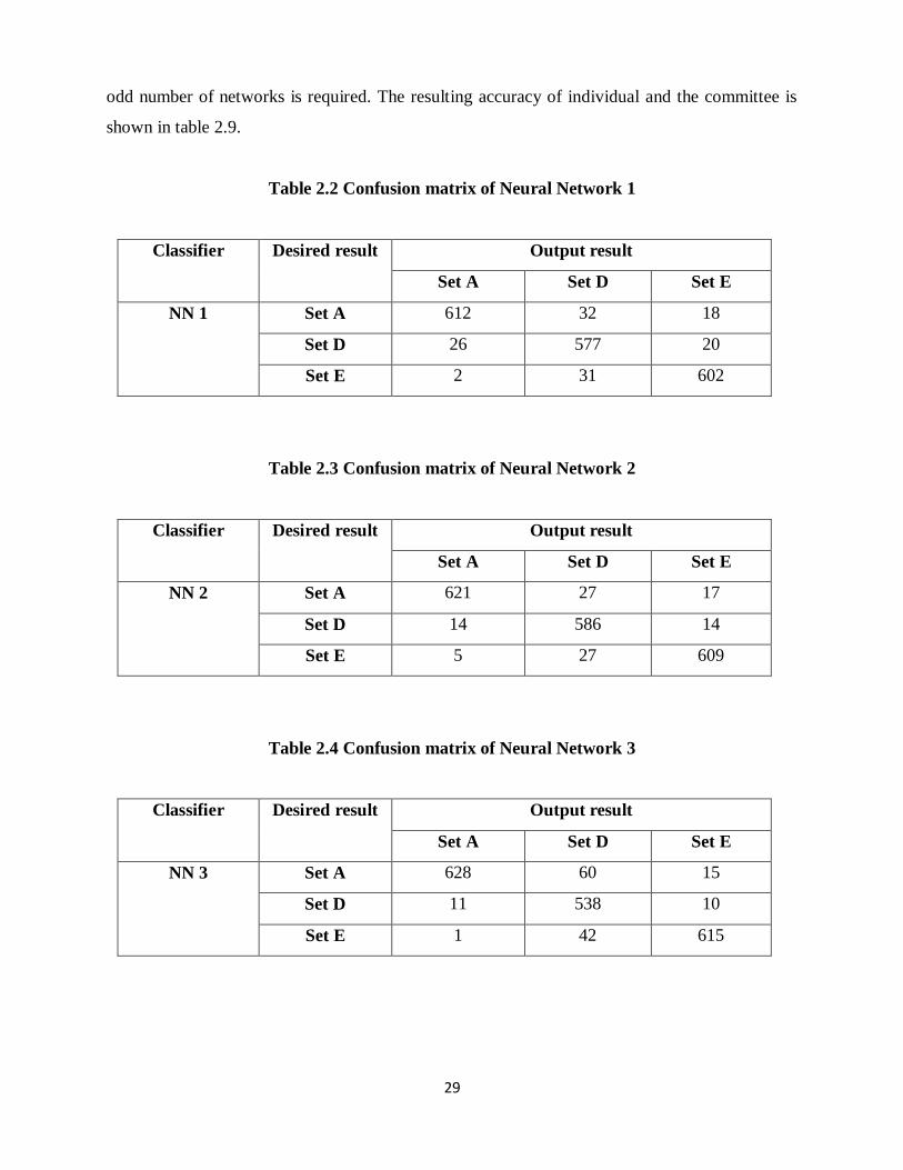
29

odd number of networks is required. The resulting accuracy of individual and the committee is

shown in table 2.9.

Table 2.2 Confusion matrix of Neural Network 1

Classifier Desired result Output result

Set A Set D Set E

NN 1 Set A 612 32 18

Set D 26 577 20

Set E 2 31 602



Set A Set D Set E

NN 2 Set A 621 27 17

Set D 14 586 14

Set E 5 27 609



Set A Set D Set E

NN 3 Set A 628 60 15

Set D 11 538 10

Set E 1 42 615

30

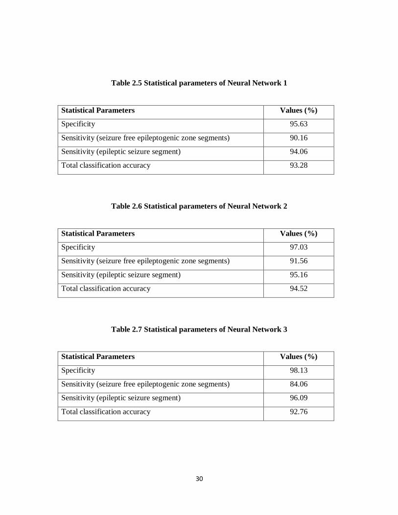
Table 2.5 Statistical parameters of Neural Network 1

Statistical Parameters Values (%)

Specificity 95.63

Sensitivity (seizure free epileptogenic zone segments) 90.16

Sensitivity (epileptic seizure segment) 94.06

Total classification accuracy 93.28



Specificity 97.03






Specificity 98.13




31

Table 2.8 Statistical parameters of Committee Neural Network


Specificity 98.02




Table 2.9 Accuracy of Committee neural network

ANN Accuracy

NN1 93.28

NN2 94.52

NN3 92.76

CNN 95.31

The outputs of the member MLPNN of the committee were represented by unit basis vectors: i.e.

[0 0 1] = healthy segments (set A)

[0 1 0] = seizure free epileptogenic zone segments (set D)

[1 0 0] = epileptic seizure segments (set E)

The statistical parameters are defined as follows:

Specificity: Number of correctly classified healthy segments/ Total number of healthy segments.

Sensitivity (seizure free epileptogenic zone segments): Number of correctly classified seizure

free epileptogenic zone segments/ Total number of seizure free epileptogenic zone segments.

Sensitivity (epileptic seizure segments): Number of correctly classified epileptic seizure

segments/Total number of epileptic seizure segments.

Total classification accuracy: Number of correct classified segments/ total number of

segments[22].

The committee neural network achieves better performances than individual members with

accuracy of 98.02%, 91.82% and 96.09% for set A, D and E respectively and overall accuracy of

95.31%.

32

Chapter 3

Dimension Reduction

using F-Ratio based

Technique

33

3.1 F-Ratio

F-Ratio is a statistical measure which is used in the comparison of statistical models that have

been fit to data set to identify the model that best fits the population from which the data were

sampled [21]. We can see a multi cluster data as shown in fig 3.1. F-ratio can be formulated as

𝐹 − 𝑟𝑎𝑡𝑖𝑜 =𝑉𝑎𝑟𝑖𝑎𝑛𝑐𝑒 𝑜𝑓 𝑚𝑒𝑎𝑛 𝑏𝑒𝑡𝑤𝑒𝑒𝑛 𝑡𝑕𝑒 𝑐𝑙𝑢𝑠𝑡𝑒𝑟𝑠

𝐴𝑣𝑒𝑟𝑎𝑔𝑒 𝑣𝑎𝑟𝑖𝑎𝑛𝑐𝑒 𝑤𝑖𝑡𝑕𝑖𝑛 𝑡𝑕𝑒 𝑐𝑙𝑢𝑠𝑡𝑒𝑟

µ3

µ2µ1

clustersmean

global

mean

cluster 1 cluster 2

cluster 3

µ0

Figure 3.1: Diagram for multi-cluster data

Suppose there are k numbers of clusters each having n number of data points. If xij is an

ith element of the j

th class then the mean of the j

th class µj can be expressed as [26]

𝜇𝑗 =1

𝑛 𝑥𝑖𝑗

𝑛

𝑖=1

The mean of all µj is called the global mean of the data and can be expressed as µ0

𝜇0 =1

𝑘 𝜇𝑗

𝑘

𝑗 =1

34

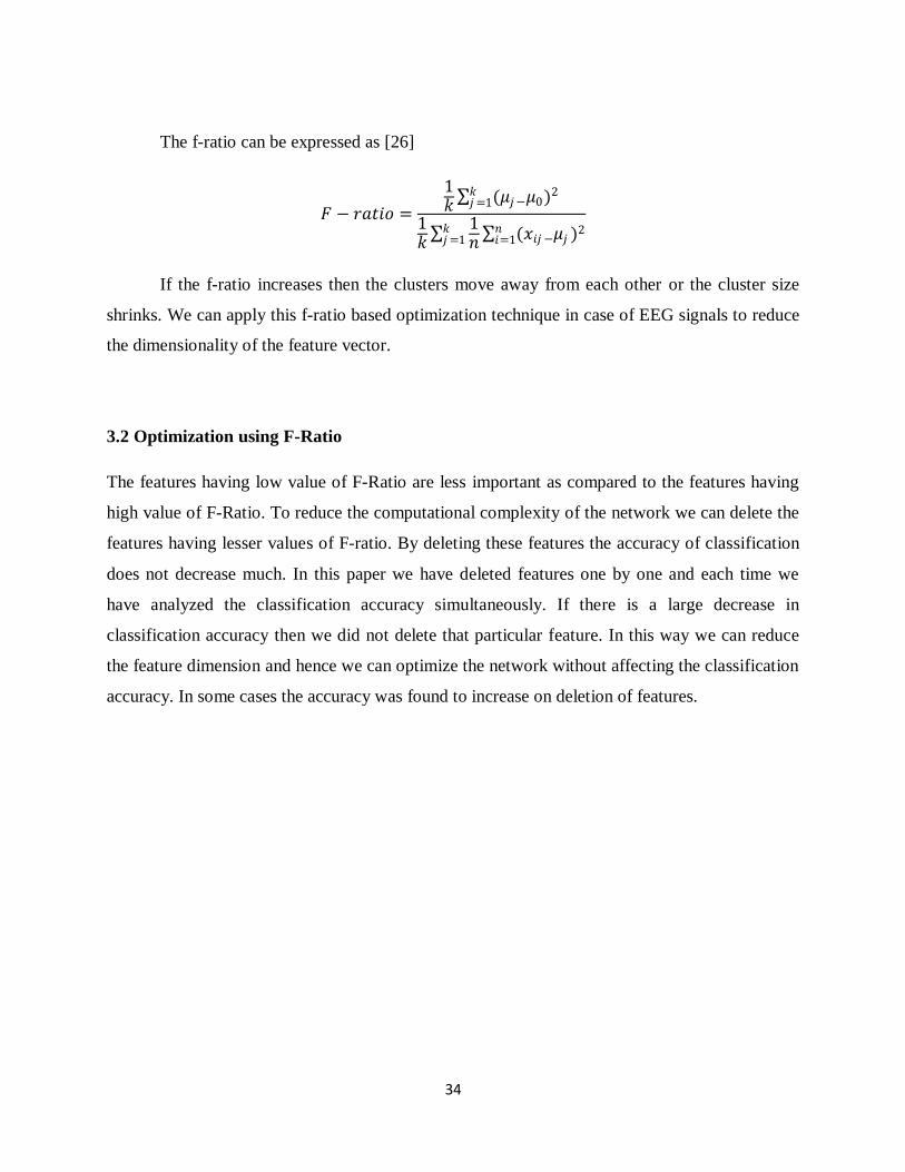
The f-ratio can be expressed as [26]

𝐹 − 𝑟𝑎𝑡𝑖𝑜 =

1𝑘

(𝜇𝑗−𝜇0)2𝑘𝑗 =1

1𝑘

1𝑛

(𝑥𝑖𝑗 −𝜇𝑗 )2𝑛𝑖=1

𝑘𝑗 =1

If the f-ratio increases then the clusters move away from each other or the cluster size

shrinks. We can apply this f-ratio based optimization technique in case of EEG signals to reduce

the dimensionality of the feature vector.

3.2 Optimization using F-Ratio

The features having low value of F-Ratio are less important as compared to the features having

high value of F-Ratio. To reduce the computational complexity of the network we can delete the

features having lesser values of F-ratio. By deleting these features the accuracy of classification

does not decrease much. In this paper we have deleted features one by one and each time we

have analyzed the classification accuracy simultaneously. If there is a large decrease in

classification accuracy then we did not delete that particular feature. In this way we can reduce

the feature dimension and hence we can optimize the network without affecting the classification

accuracy. In some cases the accuracy was found to increase on deletion of features.

35

3.3 F-Ratio of the extracted features

The F-Ratio corresponding to each feature is shown in table 3.1.

Table 3.1 F-Ratio of the extracted features

Now in order to reduce the dimension of the feature vector features having less F-Ratio were

deleted. In the table 3.2 we have shown that the accuracy after the deletion of features.

Serial

No.

Coefficient

No.

Coefficients

F-ratio

Serial

No.

Coefficient

No.

Coefficients

F-ratio

1 21 1.082 17 1 0.226

2 22 0.9316 18 13 0.1972

3 12 0.5243 19 14 0.1958

4 8 0.4748 20 31 0.1634

5 24 0.4714 21 28 0.1555

6 9 0.4464 22 27 0.0459

7 6 0.4073 23 20 0.0444

8 10 0.401 24 26 0.0407

9 23 0.3981 25 17 0.0036

10 4 0.3915 26 18 0.0023

11 25 0.3708 27 19 0.0011

12 5 0.3699 28 11 0.0004

13 30 0.365 29 15 0.0003

14 16 0.301 30 3 0.0002

15 29 0.2875 31 7 0.0001

16 2 0.2766 x x x

36

Table 3.2 dimension reduction using F-Ratio

Hence on the basis of F-Ratio based optimization technique 18 features were deleted.

Thus computational complexity was reduced without affecting the accuracy much.

Serial No. No. of coefficients taken Network structure Accuracy %

1 31 31-93-3 95.31

2 30 30-90-3 94.91

3 29 29-87-3 95.00

4 28 28-84-3 94.71

5 27 27-81-3 94.79

6 26 26-78-3 95.03

7 25 25-75-3 95.32

8 24 24-72-3 95.02

9 23 23-69-3 95.12

10 22 22-66-3 95.37

11 21 21-63-3 94.95

12 20 20-60-3 95.16

13 19 19-57-3 95.45

14 18 18-54-3 95.29

15 17 17-51-3 95.70

16 16 16-48-3 95.83

17 15 15-45-3 95.15

18 14 14-42-3 95.04

19 13 13-39-3 94.35

37

Chapter 4

Conclusions and Future

Work

38

Conclusion

The EEG signals was collected from [9], visual inspection of the three classes does not

provide much information regarding the health of individual. So we have proceeded with the

following methods

Feature extraction was done using discrete wavelet transform and the power spectral

density was estimated by Burg‟s algorithm for AR model.

To reduce the number of wavelet coefficients we have used the statistics, viz. maximum,

minimum, mean, and standard deviation for each of the detail and the approximate

coefficients.

The AR coefficients were appended to the discrete wavelet coefficients to form the

feature vector.

We have used Committee neural network for the classification purpose. The Committee

neural network consisted of three member neural networks which were trained using

error back propagation algorithm.

The Committee neural network gives robust performance as compared to the individual

networks.

We have used the F-Ratio based optimization technique to reduce the dimension of

feature vector.

Finally using our proposed technique we have successfully classified the EEG signals

and reduced the computational complexity of the classifier.

39

Future Work

EEG signal processing promises to be a vast area of research. The technique of

committee neural network is a novel approach to improve the classification

accuracy. The process of combining the outputs of each member from the

committee implemented in this project was based on majority decision.

There are many new methodologies that can be implemented in this area. Further

different types of classifiers can be tested using different EEG database.

Other feature extraction techniques can be tried so that a best possible set of

features can be used also to reduce the computational complexity other

dimensionality reduction techniques can be applied to the feature vectors.

40

REFERENCES

[1]. Saeid Sanei and J.A. Chambers, EEG Signal Processing, John Wiley & Sons Ltd, England,

2007.

[2]. Attwood, H. L., and MacKay, W. A., Essentials of Neurophysiology, B. C. Decker,

Hamilton, Canada,1989.

[3]. Teplan, M., “Fundamentals of EEG measurements”, Measmt Sci. Rev., vol. 2, 2002.

[4]. Jasper, H., „Report of committee on methods of clinical exam in EEG‟, Electroencephalogr.

Clin. Neurophysiol., vol. 10, 1958, 370–375.

[5]. Niedermeyer, E., “The normal EEG of the waking adult”, Chapter 10, in

Electroencephalography, Basic Principles, Clinical Applications, and Related Fields, Eds E.

Niedermeyer and F. Lopes da Silva, 4th edn, Lippincott, Williams and Wilkins, Philadelphia,

Pennsylvania, 1999, 174–188.

[6]. Sterman, M. B., MacDonald, L. R., and Stone, R. K., „Biofeedback training of sensorimotor

EEG in man and its effect on epilepsy‟, Epilepsia, 15, 1974, 395–416.

[7]. Ashwal, S., and Rust, R., „Child neurology in the 20th century‟, Pedia. Res., 53, 2003, 345–

361.

[8]. Pfurtscheller, G., Flotzinger, D., and Neuper, C., “Differentiation between finger, toe and

tongue movement in man based on 40 Hz EEG”, Electroencephalogr. Clin. Neurophysiol., vol.

90, 1994, 456–460.

[9]. http://www.meb.uni-bonn.de/ epileptologie/science/physik/eegdata.html

41

[10]. R.G. Andrzejak, K. Lehnertz, F. Mormann, C. Rieke, P. David, C.E. Elger, Indications of

nonlinear deterministic and finite-dimensional structures in time series of brain electrical

activity: dependence on recording region and brain state, Physical Review E 64 (2001) 061907.

[11]. http://www.dtic.upf.edu/~xserra/cursos/TDP/referencies/Park-DWT.pdf

[12]. M. Unser, A. Aldroubi, A review of wavelets in biomedical applications, Proceedings of

the IEEE 84 (4) (1996) 626–638.

[13]. I. Daubechies, The wavelet transform, time-frequency localization and signal analysis,

IEEE Transactions on Information Theory 36 (5) (1990) 961–1005.

[14]. S. Soltani, “On the use of the wavelet decomposition for time series prediction”,

Neurocomputing 48 (2002) 267–277.

[15]. İnan Güler, Elif Derya Übeyli, Adaptive neuro-fuzzy inference system for classification of

EEG signals using wavelet coefficients, Journal of Neuroscience Methods, Volume 148, Issue 2,

30 October 2005, Pages 113-121.

[16]. Unser M, Aldroubi A., A review of wavelets in biomedical applications, Proc IEEE 1996;

vol. 4, 626–38.

[17]. Narender P. Reddy, Ojas A. Buch, “Speaker verification using committee neural networks”,

Computer Methods and Programs in Biomedicine, Volume 72, Issue 2, October 2003, Pages

109-115

[18]. S. Haykin, Neural Networks: A Comprehensive Foundation, Macmillan, New York, 1994.

[19]. Sharkey, A.J.C., 1996. “On combining artificial neural nets”. Connect. Sci. 8,

pages 299–314.

http://www.dtic.upf.edu/~xserra/cursos/TDP/referencies/Park-DWT.pdf

http://www.sciencedirect.com/science?_ob=ArticleURL&_udi=B6T5J-4728BVY-1&_user=1657113&_coverDate=10%2F31%2F2003&_alid=1328634914&_rdoc=1&_fmt=high&_orig=search&_cdi=5004&_docanchor=&view=c&_ct=1356&_acct=C000053917&_version=1&_urlVersion=0&_userid=1657113&md5=73cd261e5063787d92d042952ca62f0d

42

[20] The "10–20 system" of electrode placement. The University of Washington.

http://faculty.washington.edu/chudler/1020.html. Accessed on 14 January 2003.

[21] http://en.wikipedia.org/wiki/Eeg

[22] Elif Derya Übeyli, “Statistics over Features: EEG signals analysis”,

Computers in Biology and Medicine, Volume 39, Issue 8, August 2009, Pages 733-741

[23] John G. Proakis , Dmitris G. Manolakis, Digital Signal Processing, Pearson Education,

Fourth Edition.

[24] J. P. Burg, “Maximum entropy spectral analysis”, in Proc. 37th

Meeting Soc. Exploration

Geophys., 1967

[25] P. Stoica and R. L. Moses, Introduction to spectral Analysis. Upper Saddle River, NJ:

Prentice-Hall, 1997.

[26] Goutam Saha, Sandipan Chakroborty, Suman Senapati, “An F-Ratio based optimization

technique for automatic speaker recognition system” IEEE India Annual Conference 2004,

INDICON 2004.

http://faculty.washington.edu/chudler/1020.html

analysis and classification of electroencephalography signals · 2019-01-02 · analysis and...

Documents