analysis and design of - core.ac.uk · analysis and design of ultra-wideband transceiver and array...

ANALYSIS AND DESIGN OF

ULTRA-WIDEBAND TRANSCEIVER AND ARRAY

ADRIAN TAN ENG CHOON

(B. Eng. (Hons.), NUS)

A THESIS SUBMITTED

FOR THE DEGREE OF DOCTOR OF PHILOSOPHY

NUS GRADUATE SCHOOL FOR INTEGRATIVE

SCIENCES AND ENGINEERING

NATIONAL UNIVERSITY OF SINGAPORE

2007

To My Wife

ACKNOWLEDGMENT iv

ACKNOWLEDGMENT

I would like to express my deepest gratitude to my supervisor, Adj. A/P Michael Chia Yan

Wah, who has given me the invaluable opportunity to study under his guidance. His realistic

attitude towards research and engineering has influenced me considerably. I would also like to

sincerely thank each of my committee members, Adj. A/P Chen Zhining and A/P Li Le-Wei for

their encouragements in times of difficulty.

I would like to thank Dr. Karumudi Rambabu, who has aided me in many ways, and is a role

model to me to pursue a career in academic research. I would like to thank all my friends in the

Institute for Infocomm Research: Kevin Chan Khee Meng, Leong Siew Weng, Sim Chan Kuen,

Seah Kwang Hwee and Terence See Shie Peng. I would also like to thank the staff in the Radio

System Department, Information System Department and NUS Graduate School for their kind

support.

I would like to thank my friends who have taught me many lessons in life over the years of

my hostel life in secondary school, junior college and university. I would also like to express my

gratitude to the Ministry of Education, National University of Singapore, and the Agency for

Science and Technology Research, who have provided me the opportunity and financial support

for my education in Singapore.

Finally and most importantly, I want to thank my family members: my wife for her love and

dedication, my father and mother for making the right decisions, for the endless support and

patience in seeing me through my life and education, and my brother whom we have shared many

life experiences.

ABSTRACT v

ABSTRACT

Ultra wideband (UWB) is a new emerging short-range device technology with potential

benefits for wireless communications, radars, localization, tracking and security applications.

UWB systems exchange information by transmitting and receiving short electromagnetic pulses.

Therefore, it is very essential to understand the pulse transmission, propagation and reception by

UWB terminals. Fundamentally, pulse radiation is different from narrowband signals. Hence,

understanding the pulse radiation, effect of the antenna on pulse shape, and signal distortion by

band-limited channel are the high priority goals of UWB technology developers. This thesis

presents the derivation of the impulse response of an antenna in both transmitting and receiving

modes to evaluate the effect of the antenna on UWB pulse shape. This thesis also discusses the

development of a UWB signal source that generates sub-nanosecond pulses. Lastly, this thesis

presents the system designs for UWB angle-of-arrival (AOA) receivers, UWB monopulse

receivers, and medical imaging UWB radars.

In Chapter 2, the impulse response of an antenna in transmitting and receiving modes is

derived based on the field distribution of the antenna aperture. To validate the proposed theory,

the impulse response for a ridged-horn antenna is derived, and the transmitted and received UWB

pulses are studied. The UWB pulses are then measured, and are found to be in good agreement

with the proposed theory. This study also discusses the effect of band-limited channel and angular

dependence of the received UWB pulses. Chapter 3 applies the impulse response of the antenna

into the derivation of the received signals of a UWB time-difference-of-arrival (TDOA) receiver.

The UWB TDOA receiver is then analyzed to derive its accuracy in estimating the angle-of-

ABSTRACT vi

arrival (AOA) of a target in the presence of antenna noise. The derived angle accuracy is verified

with root-mean-square errors of AOA measurements using a prototype of the UWB TDOA

receiver. From the analysis and measurement, it is found that the angle accuracy of the UWB

TDOA receiver depends not only on signal-to-noise ratio but also on angle of incidence.

Chapter 4 details the derivation of the impulse response of a UWB monopulse receiver. The

monopulse receiver uses a square-feed array of ridged-horn antennas to capture the incident

signal. A bank of cross-correlation receivers is proposed to receive the monopulse signals to

enable angle discrimination of the UWB monopulse receiver. The output voltages from the cross-

correlators are used to find the target angle with an amplitude-comparison monopulse processor.

The derivations are verified with measurements of monopulse signals and the output voltages of

the cross-correlators. The angle accuracy of the UWB monopulse receiver in the presence of

antenna noise is also examined.

Chapter 5 presents the design, fabrication and measurement of a UWB pulse-forming

network (PFN) that is amenable to integrated circuits. The designed PFN is suitable for

applications in high data rate UWB communication systems and short-range UWB radars. To

generate a UWB pulse, a frequency-selective, negative-feedback circuit to perform time

derivative on an input step signal is used. Measured output pulses of the proposed PFN show

consistency in pulse widths (170 ps to 180 ps) for a large variation of input signal rise-times (45

ps to 300 ps), as intended by the design. The PFN consumes 3.3 V, 20 mA during operation.

In Chapter 6, a method for imaging the human body using UWB radars is proposed. The

method uses the scattered signals from the human body to calculate its impulse response. Human

phantoms are fabricated. Impulse responses of the human phantoms are measured with a

prototype of UWB radar. The measured impulse responses of the human phantoms are verified by

comparing them with derived reflection coefficient of an infinitely large two-layered medium. It

is found that the UWB radar can achieve limited imaging capability of the internal organs in the

human body.

CONTENTS vii

CONTENTS

Title Page i

Dedication iii

Acknowledgement iv

Abstract v

Table of Contents vii

List of Figures x

List of Tables xv

List of Symbols xvi

List of Contributions xx

1 Introduction 1

1.1 Research background and related work 1

1.2 Contributions 8

1.3 Thesis organization 11

2 Transmission and Reception of Ultra-Wideband Pulses 13

2.1 Chapter introduction 13

2.2 Transmitting and receiving characteristics of an aperture antenna 14

2.3 Transmission and receiving characteristics of ridged-horns 19

2.4 Experimental verification: Impulse response of antenna in receiving mode 21

CONTENTS viii

2.5 Experimental verification: Impulse response of antenna in transmitting mode 29

2.6 Chapter summary 36

3 Antenna Noise Effect on Ultra-Wideband Angle Estimation 38


3.2 Time-of-arrival estimation of UWB signals at boresight 39

3.3 Time-of-arrival estimation of UWB signals at off-boresight 42

3.4 Angle-of-arrival estimation of UWB TDOA receivers 46

3.5 Verification of time-of-arrival derivations 49

3.6 Numerical simulation of angle-of-arrival 54

3.7 Measurement of angle-of-arrival 57


4 Design of Ultra-Wideband Monopulse Receiver 64


4.2 Impulse response of monopulse square-feed array 65

4.3 Monopulse receiver 70

4.4 Monopulse waveform measurements 78

4.5 Angle-of-arrival accuracy measurements 85


5 Sub-nanosecond Pulse Forming Network for UWB Transceiver 93


5.2 Schematic design of the pulse forming network 95

5.2.1 System requirement of the pulse forming network 96

5.2.2 Circuit to enhance the input signal 98

5.2.3 Circuit to differentiate the input signal 100

5.3 Circuit implementation and measurements 104

5.4 Measurement result 107

5.4.1 Pulse shape 107

5.4.2 Power spectral density 109


CONTENTS ix

6 Measuring Human Body’s Impulse Response with Ultra-Wideband Radar 114


6.2 Measurement theory 115

6.3 Modeling the human body’s impulse response 121

6.4 Construction of human phantom and UWB radar 124

6.5 Measured result 129


7 Conclusion 135

7.1 Conclusion 135

7.2 Future work 137

8 Bibliography 139

LIST OF FIGURES x

LIST OF FIGURES Figure:

1.1 Transmitter schematics of a non-impulse based UWB radio system. 2

1.2 Transmitter schematics of an impulse based UWB radio system. 2

2.1 Antenna aperture (grey rectangle) and a point, P, in the far field distance. 15

2.2 Picture of the double-ridged horn by RCM Ltd. (model MDRH-1018). 19

2.3 The ridged-horn’s aperture dimensions and a typical aperture field distribution (dashed line) of the ridged-horn.

20

2.4 Experimental setup for time-domain measurement of received signal at different angles.

23

2.5 Measured (line) and modeled (dashed line) transmitted UWB pulse. 24

2.6 A picture of the transmitter setup in the measurement. 25

2.7 A picture of the receiver setup in the measurement. 25

2.8 Measured (line) and modeled (dashed line) received signal in the azimuth plane. 27

2.9 Measured (line) and modeled (dashed line) received signal in the elevation plane. 27

2.10 Measured (crosses) and modeled (line) normalized energy pattern in the azimuth plane.

28

2.11 Measured (crosses) and modeled (line) normalized energy pattern in the elevation plane.

29

2.12 Transfer functions used to model the transmission and reception of UWB pulses. 30

2.13 Measured (line) and theoretical (dashed line) UWB source signal. 32

2.14 Measured (line) and theoretical (dashed line) transfer functions used to model the transmitting antenna’s frequency-limited gain, Ht (ω), attenuation due to propagation in free-space, Hch (ω) and the receiving antenna’s frequency-limited gain, Hr (ω).

33

2.15 Measurement setup used to measure the received UWB signal. 35

2.16 Measured (line) and modeled (dashed line) received signal in the azimuth plane. 36

LIST OF FIGURES xi

3.1 Schematic of a stored reference cross-correlation receiver estimating the time-of-arrival of a received signal.

40

3.2 A UWB cross-correlation receiver. 42

3.3 A UWB Time-difference-of-arrival (TDOA) receiver array. 46

3.4 A sample of measured received signal with antennas RH1 and RH2. 50

3.5 Measured received signal with antennas RH1 (dotted line) and RH2 (dashed line) compared to the modeled received signal (line) in three power levels.

51

3.6 A sample of measured noise signal of antennas RH1 and RH2. 52

3.7 Theoretical standard deviations of estimated angle-of-arrival (AOA) for three cases of signal-to-noise ratio (SNR).

55

3.8 Schematic of simulation process to verify TDOA receiver’s angle-of-arrival accuracy.

55

3.9 Simulated standard deviations of estimated angle-of-arrival (AOA) for three cases of signal-to-noise ratio (SNR).

56

3.10 Angle-of-Arrival measurement setup. 57

3.11 Picture of Angle-of-Arrival measurement setup. 58

3.12 Measured received signals and correlator outputs for antennas RH1 and RH2 at θ = +10°, Case 2 SNR.

59

3.13 Distribution of measured Angle-of-Arrival (AOA) for θ = 10° (line) and other angles (dotted lines).

59

3.14 Theoretical, simulated and measured standard deviations of angle of arrival (AOA) estimation for Case 1 SNR.

62


62


63

4.1 Monopulse receiver coordinate systems and antenna dimensions. 66

4.2 Monopulse comparator circuit with four 180° hybrid-couplers. 66

4.3 Plot of experimental (line) and modeled (dotted line) incident signal. 71

4.4 Block diagram of UWB monopulse receiver. 73

LIST OF FIGURES xii

4.5 Theoretical, measured and approximate difference signal in the azimuth plane for θ = θA ≈ 3.9°.

76

4.6

Experimental setup to measure the received monopulse sum and difference signals. 78

4.7 Comparison between measured normalized gain pattern of a single ridged-horn with the normalized gain patterns derived from various theoretical aperture functions.

79

4.8 Comparison between simulated (dotted line) and measured (line) sum signals for θ = -20°, -10°, 0°, 10° and 20°.

81

4.9 Comparison between simulated (dotted line) and measured (line) difference signals for θ = -20°, -10°, 0°, 10° and 20°.

81

4.10 Theoretical and measured (line) monopulse sum channel cross-correlation output. The theoretical monopulse sum outputs are calculated based on rectangular aperture function (dotted line) and cos12 aperture function (dashed line).

82

4.11 Theoretical and measured monopulse difference channel cross-correlation output. The theoretical monopulse sum outputs are calculated based on rectangular aperture function (dotted line) and cos12 aperture function (dashed line).

82

4.12 Comparison between theoretical (line) and measured (circles) monopulse ratio. The theoretical (line) monopulse ratio is derived based on ridged-horn aperture functions that are defined by cos12 functions.

83

4.13 The effect of the antenna aperture length on the Monopulse ratio and the performance of the Monopulse tracking receiver.

84

4.14 The effect of the incident signal’s pulse-width on the Monopulse ratio and the performance of the Monopulse tracking receiver.

85

4.15 Comparison between theoretical (line) and measured (circles) standard deviations of time-of-arrival (TOA) for different angles.

87

4.16 Theoretical (line) and measured (circles) standard deviations of angle error for Eb / N0 of 28.5 dB.

92

5.1 A time domain UWB transceiver using the pulse forming network in the transmitter and receiver.

94

5.2 Schematic diagram of a time domain UWB transmitter using the pulse forming network.

96

5.3 Schematic diagram of a time domain UWB radar using the pulse forming network. 97

LIST OF FIGURES xiii

5.4 Schematics diagram of the input signal enhancing circuit. 99

5.5 Plot of output positive step rise-time (o) and output negative slope rise-time (x) for a input step rise-time.

100

5.6 Negative feedback used to realize the differentiator block. 100

5.7 The proposed differentiator circuit. 101

5.8 Small signal analysis of the proposed differentiator circuit. 102

5.9 Frequency response of the small signal equivalent circuit (theoretical) and schematics (simulated) shows linear gain at frequencies 1 – 10 GHz.

102

5.10 Frequency domain simulation of the feedback voltage, vf, shows that the gain variation of vf is less than 1 dB at 10 GHz (Trace 1), and the phase variation of vf is less than 50º (Trace 2).

103

5.11 Magnified picture of the fabricated circuit. 104

5.12 Picture of the PCB board used for testing purposes, and the IC chip. 105

5.13 Schematics of test setup for time domain measurement of the PFN output. 105

5.14 Schematic of the test setup for the EIRP measurement of a transmitter with the fabricated PFN.

106

5.15 Comparison between theoretical, simulated and measured pulse shape of the PFN for an input data signal of 40 ps rise-time.

107

5.16 Output of the PFN when input signal is a highly distorted 500 MHz clock signal with 300 ps rise-time.

108

5.17 Measured time-domain signals at various stages of the transceiver system in Figure 5.13.

109

5.18 Measured spectral content of PFN output shows that it contains sufficient spectral power for UWB signal from 3.1 – 10.6 GHz.

110

5.19 Measured spectral content of 3 – 6 GHz bandpass filtered output of the PFN. 110

5.20 Measured EIRP of the transmitter. 111

5.21 Comparison between the FCC emission limit and the measured EIRP for Manchester coded an alternate bit [1,0] sequence and a pseudo-random bit sequence.

112

6.1 A monostatic UWB radar detecting a target and the linear transfer function model used to model the detection process.

116

LIST OF FIGURES xiv

6.2 A UWB radar (Receiver) capturing a transmitted signal from a similar UWB radar (Transmitter), and the linear transfer function used to model the process.

118

6.3 Signal processing blocks implemented in ADS Ptolemy [62] simulation to compute the impulse response of target.

120

6.4 Reflection diagram of a UWB signal incident on a target consisting of a two layer medium.

121

6.5 Transmission-line analogy of the wave propagation modeled in Figure 6.4. 123

6.6 Heart cross-section of the human torso [76]. 124

6.7 Stomach cross-section of the human torso [76]. 125

6.8 Dielectric values, at 6 GHz, of measurement phantom (underlined) are comparable to that of selected human body tissues.

126

6.9 Human body phantom construction, positioning and measurement. 126

6.10 Schematic diagram of the UWB radar. 127

6.11 Transmitted UWB signal, measured with a ridged-horn antenna at far-field. 128

6.12 Power spectral density (normalized) of a transmitted UWB signal. 129

6.13 Measured signal of 10 mm palm oil human phantom, and the impulse responses with different values of ωc.

130

6.14 Measured signal (line), measured impulse response (line) and theoretical impulse response (dashed line) of 32 mm layer of palm oil (cooking oil).

131

6.15 Measured signal (line), measured impulse response (line) and theoretical impulse response (dashed line) of 9 mm layer of GSM 1800 brain tissue simulant.

131

6.16 Measured signal (line), measured impulse response (line) and theoretical impulse response (dashed line) of 8 mm layer of saturated sugar solution.

132

6.17 Measured signal (line), measured impulse response (line) and theoretical impulse response (dashed line) of 9 mm layer of tap water.

132

LIST OF TABLES xv

LIST OF TABLES

Table:

3.1 Theoretical and experimental time-of-arrival standard deviation at boresight for six cases of SNR.

53

3.2 Theoretical and experimental time-of-arrival standard deviation at ± 10° for six cases of SNR.

53

3.3 Theoretical and experimental time-of-arrival standard deviation at ± 20° for six cases of SNR.

54

3.4 Measured mean and standard deviation of angle-of-arrival for the three cases of SNR.

60

LIST OF SYMBOLS xvi

LIST OF SYMBOLS

Ach Propagation channel’s frequency independent attenuation

Ae Amplitude of the incident signal

As Amplitude of the source signal

d1 Antenna dimension at the x’ direction

d2 Antenna dimension at the y’ direction

de Delay of the source signal

ds Delay of the incident signal

dmi Thickness of medium i

DA (θ, φ) Azimuth difference channel cross-correlated voltage value

DE (θ, φ) Elevation difference channel cross-correlated voltage value

D Estimated azimuth difference channel cross-correlated value

c Speed of light in vacuum

e (t), E (ω) Incident signal to the receiving antenna

Eb Energy of the received signal

Ed (θ) Energy of the received signal in the azimuth difference channel

Es (θ) Energy of the received signal in the sum channel

fc (t), Fc (ω) Transfer function of signal propagation at path ‘C’

fe (t), Fe (ω) Transfer function of signal propagation at path ‘E’

fσ (t), Fσ (ω) Transfer function of the scattering from the target

fwσ (t), Fw

σ (ω) Windowed transfer function of the scattering from the target

fthσ (t), Fth

σ (ω) Theoretical transfer function of the scattering from the target

LIST OF SYMBOLS xvii

fad (t, θ, φ), Fad (ω, θ, φ) Impulse response of the azimuth difference array in receiving mode

fed (t, θ, φ), Fed (ω, θ, φ) Impulse response of the elevation difference array in receiving mode

fs (t, θ, φ), Fs (ω, θ, φ) Impulse response of the Sum array in receiving mode

ft (t, θ, φ), Ft (ω, θ, φ) Impulse response of the antenna in transmitting mode

fr (t, θ, φ), Fr (ω, θ, φ) Impulse response of the antenna in receiving mode

g (x’, y’) Field distribution of antenna aperture

g1 (x’) Field distribution of antenna aperture in the x’ axis

g2 (y’) Field distribution of antenna aperture in the y’ axis

gad (x’, y’) Field distribution of azimuth difference array

ged (x’, y’) Field distribution of elevation difference array

gs (x’, y’) Field distribution of sum array

ht (t), Ht (ω) Transfer function of the transmitting antenna

hr (t), Hr (ω) Transfer function of the receiving antenna

hch (t), Hch (ω) Transfer function of the propagation channel

k0 Propagation constant of free space

ki Propagation constant of medium i

kB Boltzmann’s constant B

m Positive integer value, models the antenna field in the x’ axis

n Positive integer value, models the antenna field in the y’ axis

ni (t) Thermal noise signal of the i-th receiver

Ni Noise power per unit bandwidth of the i-th receiver

pda (t) Azimuth difference channel reference cross-correlation signal

pde (t) Elevation difference channel reference cross-correlation signal

ps (t) Sum channel reference cross-correlation signal

r (t), R (ω) Output signal of the receiving antenna

rad (t), Rad (ω) Azimuth difference signal of the Monopulse receiver

LIST OF SYMBOLS xviii

red (t), Red (ω) Elevation difference signal of the Monopulse receiver

rs (t), Rs (ω) Sum signal of the Monopulse receiver

rn (t) Noise corrupted output signal of the receiving antenna

rsn (t) Noise corrupted output signal of the sum channel

rdan (t) Noise corrupted output signal of the azimuth difference channel

r0 (t), R0 (ω) Reference correlating signal of the TDOA receiver

R Estimated Monopulse ratio

s (t), S (ω) Input signal to the transmitting antenna

s1 Separation between antennas at the x’ direction

s2 Separation between antennas at the y’ direction

S (θ, φ) Sum channel cross-correlated voltage value

S Estimated sum channel cross-correlated value

v (τ, θ) Signal function of the posterior probability of the estimated TOA

vd Signal function of the azimuth difference channel value

vs Signal function of the sum channel value

w (τ, θ) Noise function of the posterior probability of the estimated TOA

wd Noise function of the azimuth difference channel value

ws Noise function of the sum channel value

Wg (ω) Frequency windowing function

τe Pulse width of the incident signal

τs Pulse width of the source signal

T Pulse repetition interval

Tant Antenna temperature

α Length of the ridged-horn antenna

β Height of the ridged-horn antenna

LIST OF SYMBOLS xix

βs (θ) Signal’s second moment

ε0 Free space permittivity constant

θ Estimated angle of arrival of receiver

η0 Intrinsic impedance of free space

ηi Intrinsic impedance of medium i

μ0 Free space permeability constant

ωch Propagation channel’s frequency dependent attenuation

τ0 True time of arrival of received signal

0τ Estimated time of arrival of received signal

τ Sweeping delay of the reference signal, to estimate τ0

στi (θ) Standard deviation of the estimated TOA at the i-th channel

LIST OF CONTRIBUTIONS xx

LIST OF CONTRIBUTIONS

[1] A. E.-C. Tan, and M. Y.-W. Chia, “UWB Radar Transceiver and Measurement for Medical

Imaging”, IEEE BioCAS, Singapore, Dec. 2004. [2] A. E.-C. Tan, and M. Y.-W. Chia, “Method of Generating UWB Pulses”, World

Intellectual Property Organization, Pub. No. WO 2005/067160 A1, Jul. 2005. [3] A. E.-C. Tan and M. Y.-W. Chia, “Measuring Human Body Impulse Response Using

UWB Radar”, IEE Electron. Lett., vol. 41, no. 21, Oct. 2005, pp. 1193-1194. [4] A. E.-C. Tan and M. Y.-W. Chia, “Measuring Human Body’s Impulse Response”, UK-

Singapore Bioelectronics Workshop, Jan 2006. [5] A. E.-C. Tan, M. Y.-W. Chia and S.-W. Leong, “Sub-nanosecond Pulse-Forming Network

on SiGe BiCMOS for UWB Communications”, IEEE Trans. MTT, vol. 54, no. 3, Mar. 2006, pp. 1019-1024.

[6] K. Rambabu, A. E.-C. Tan, K. K.-M. Chan and M. Y.-W. Chia and S.-W. Leong, “Study of

Antenna Effect on UWB Pulse Shape in Transmission and Reception”, ISAP 2006, Singapore, Nov. 2006.

[7] A. E.-C. Tan, M. Y.-W. Chia and K. Rambabu, “Design of Ultra-Wideband Monopulse

Receiver”, IEEE Trans. MTT, vol. 54, no. 11, Nov. 2006, pp. 3821-3827. [8] K. Rambabu, A. E.-C. Tan, K. K.-M. Chan and M. Y.-W. Chia, “Estimation of Antenna

Effect on UWB Pulse Shape in Transmission and Reception”, submitted to IEEE Trans. MTT, Nov. 2006.

[9] A. E.-C. Tan, M. Y.-W. Chia and K. Rambabu, “Effect of Antenna Noise on Angle

Estimation in Ultra-Wideband Receivers”, submitted to IEEE Trans. AP, Dec. 2006. [10] A. E.-C. Tan, M. Y.-W. Chia and K. Rambabu, “Angle Accuracy of Antenna Noise

Corrupted Ultra-Wideband Monopulse Receiver”, ICUWB 2007, Sep. 2007.

CHAPTER 1 1

CHAPTER 1

INTRODUCTION

1.1 Research Background

This thesis presents the analysis and design of ultra-wideband (UWB) radio transceivers and

arrays. UWB radio transceivers can be contrasted from their narrowband radio counterparts by the

signals that they transmit and receive, which tend to be large in fractional bandwidth [1]. UWB has

been defined by the Federal Communications Commission (FCC) as radio systems that transmit

signal with fractional bandwidth larger than 0.2, or a bandwidth that is at least 500 MHz [2]. For

UWB radio systems, the fractional bandwidth is defined as 2 (fH − fL) / (fH + fL), where fH is the upper

−10 dB edge frequency and fL is the lower −10 dB edge frequency. According to the current FCC’s

frequency allocations [2], there are, in total, three frequency bands that are allowed for UWB

operations, with each band catering for different types of applications. The allotted frequency bands

are: below 960 MHz, 3.1 − 10.6 GHz and 22 − 29 GHz. For all three bands, the effective isotropic

radiated power (EIRP) is limited to −41.3 dBm / MHz.

The 3.1 − 10.6 GHz band UWB radio finds many applications in short range, high data rate

communication systems [3], [4] and in radar systems [1], [5]. Currently, there are two competing

methods to provide UWB radio communications in the 3.1 – 10.6 GHz band. They can be classified

as the impulse and non-impulse UWB radio systems. The impulse and non-impulse UWB radio

systems came about in the IEEE 802.15 Task Group 3a, where two competing technical proposals –

the multi-band orthogonal frequency division multiplexing (MB-OFDM) and direct-sequence ultra-

CHAPTER 1 2

wideband (DS-UWB), fail to reconcile their differences. The MB-OFDM is commonly referred to the

non-impulse UWB, and the DS-UWB is commonly known as the impulse UWB radio systems.

The MB-OFDM system (non-impulse UWB) is a combination of frequency hopping and OFDM

technologies [6] [7]. A block of information forms one OFDM symbol. The OFDM symbol

bandwidth is 500 MHz, and consists of a frequency multiplex of 128 sub-carriers. The OFDM symbol

interval is 312.5 ns, after which, the subsequent symbol will be transmitted over different sub-bands

determined by pre-defined frequency hopping patterns.

The DS-UWB system (impulse UWB) is based on direct-sequence spread spectrum technology [8]

[9]. Each data symbol is spread by a specific spreading code to form a transmit sequence of pulses.

Each of the pulses has 200-300 ps pulse-width, with a subsequent quiet period that depends on the

pulse repetition frequency (PRF) of the radio system.

Baseband 1

Baseband 2

LO

90°

Linear Amplifier

Baseband 1

Baseband 2

LO

90°

Linear Amplifier

Figure 1.1: Transmitter schematics of a non-impulse based UWB radio system.

BasebandPulse

FormingNetwork

BasebandPulse

FormingNetwork

Figure 1.2: Transmitter schematics of an impulse based UWB radio system.

CHAPTER 1 3

To the RF transceiver, there are two critical differences between the impulse and non-impulse

based UWB radio systems – different signal generation method and vastly different signal time-

widths. The non-impulse based UWB radio system generates the UWB signal in a similar manner as

narrowband systems, except with a few differences, as shown in Fig. 1.1. On the other hand, the

impulse based UWB radio system generates the UWB signal by either first generating short, sub-

nanosecond pulses with non-linear circuits, and then modulates them, as shown in Fig. 1.2, or

combines the two steps into an integrated UWB signal generator.

It can be seen from Figs 1.1 and 1.2 that the transmitter architecture for impulse based UWB

radio system is much simpler than that of the non-impulse based UWB system. The time-widths of

the impulse based UWB system is 200-300 ps, compared to a much longer 312.5 ns pulse width of

the non-impulse based UWB system. Hence, the design requirement of antenna, which is of particular

interest in this research, is different. Impulse based UWB system radiates and receives signals that are

electrically short compared to size of the antennas, whereas non-impulse based UWB systems do not.

The main advantage of UWB in radio communications over its narrowband counterparts can be

understood from Shannon’s link capacity formula, where it is shown that with a large bandwidth, only

a very small radiation power is needed to achieve high data rate in short ranges [1]. Furthermore,

UWB radio systems suffer much less from channel fading as compared to narrowband radio systems,

because short pulses propagating over different paths can be better distinguished by the UWB radio

receiver. On the other hand, the UWB radar has many advantages over conventional narrowband

radars. The UWB radar has better range resolution because the short pulse enables target

differentiation at smaller dimensions in the range axis [1]. Besides that, UWB radar has more

detectable materials penetration because there is a large aggregate of frequency components in the

radiated pulse. Even if a material attenuates some frequency components of the radiated pulse, other

frequency components may not be attenuated as severely. Furthermore, it is easier to recover

information of the target from reflected signal because the signal is large in bandwidth, and thus,

provides more information on the target. Lastly, if the radar signal is coded with pseudo-random bit

CHAPTER 1 4

sequence (PRBS), the transmitted signal appears noise-like to the target, thus it has a low likelihood

of being detected.

This thesis only considers the analysis and design of UWB radio transceivers in the 3.1 − 10.6

GHz band. The 3.1 − 10.6 GHz band is chosen because, firstly, it has a large fractional bandwidth of

1.09, and secondly, it has a centre frequency of 6.85 GHz. Having a large fractional bandwidth allows

the UWB radio transceiver to transmit and receive short pulses that can be easily modeled as second

or third derivative Gaussian functions. Having a centre frequency of 6.85 GHz allows the UWB radio

transceiver to transmit and receive short pulses that have sub-nanosecond pulse widths. Both

properties of the transmitted pulse (simple and short) are important for the applications considered in

this thesis – human body surveillance and tracking (Chapters 3 and 4); high pulse rate radio

communication and radar systems (Chapter 5); and human body imaging for medical purposes

(Chapter 6).

To perform surveillance and tracking using the UWB radio transceiver, short pulse widths are

needed to provide a good location tracking accuracy. Two types of transceiver architectures will be

described in this thesis. In Chapter 3, the time-difference-of-arrival (TDOA) method of target tracking

will be described, while in Chapter 4, the monopulse method of target tracking will be described. The

excellent range accuracy of the 3.1 – 10.6 GHz UWB radio system can be best illustrated with the

following example: Let a transmitted UWB signal with 0.2 ns pulse width and a 3 dB signal-to-noise

ratio (SNR) be captured by a receiver. The said receiver can achieve a range accuracy (root-mean-

square error) of less than one centimeter [10]. The accuracy calculation in the above example will be

further elaborated in Chapter 3. To achieve an accurate imaging capability of the human body, as

shown in Chapter 6, the UWB radio transceiver will require a higher signal-to-noise ratio (SNR),

which can be achieved by signal averaging.

The thesis addresses both general and specific problems in the design of UWB radio systems.

Chapters 2, 3 and 4 of the thesis address general problems like the modeling of signal distortion by

the UWB antenna, the application of a UWB antenna array to estimate target locations and the

CHAPTER 1 5

estimation of the accuracy of such UWB radio systems. Chapters 5 and 6 address problems that are

relevant to the understanding of specific UWB radio systems, like the problem of high data rate pulse

generation and the application of UWB radar in medical imaging.

Despite the many advantages of UWB over conventional narrowband radio transceivers, many

aspects of the UWB are still insufficiently modeled. For instance, it is observed that the transmission

and reception of UWB signals suffer from varying degrees of pulse distortions at different angles

[11]−[13]. Conventional antenna parameters like antenna gain and radiation pattern [14], while

successful in explaining the transmission and reception of narrowband signals, fail to account for the

angle dependent pulse distortions in UWB signals. Because of the differences in signal transmission

and reception compared to narrowband, the UWB antenna has been modeled as an impulse response

in many existing literature [12], [15]−[19]. Schantz [20] attributed the UWB antenna’s dispersion to

the current radiation at different parts of the antenna. A more severe form of dispersion in UWB

antenna is evident in frequency independent antennas. The dispersion in these antennas are caused by

their reliance on different radiating, narrowband elements, located at different locations, to achieve

the broadband. Because of the electrically short UWB signal compared with the antenna dimension,

whenever the antenna radiates the signal at different antenna locations, signal dispersion occurs, and

needed to be accounted for. In the thesis, signal dispersion for directional antennas at different angles

will be modelled and accounted for. Furthermore, it has been shown [21]−[23] that the transmitting

transient response of an antenna is proportional to the time derivative of the receiving transient

response of the same antenna. To better model the transmission and reception of UWB signals by the

antenna, an impulse response model that relates the signal distortions by the antenna with the

antenna’s aperture field distribution is described in Chapter 2 of the thesis.

One of the ways to perform surveillance and tracking using UWB radio transceivers is with the

time-difference-of-arrival (TDOA) method [24]−[28]. The TDOA method, as described in Chapter 3

of this thesis, finds the location of the target by estimating the range and angle-of-arrival of the target.

Using the TDOA method for UWB radio systems is ideal, because the TDOA method can leverage on

CHAPTER 1 6

the inherently short electrical lengths of UWB signals in free-space (e.g. 6 to 15 cm for a UWB pulse

of typical pulse width 0.2 to 0.5 ns) to locate the radar target or transponder with better accuracy.

However, in the existing literature, analyses of UWB TDOA receivers fail to consider the antenna

impulse response effect on the receiver, which may compromise accuracy of the estimated target

location. In Chapter 3, the antenna impulse response is incorporated in the analysis of the UWB

TDOA receiver in estimating the angle-of-arrival accuracy. With the knowledge of the UWB TDOA

receiver’s accuracy, location accuracy of a target can now be a design parameter of the UWB radio

system.

In Chapter 4, we present another UWB transceiver array design that performs surveillance and

tracking. The proposed transceiver is the UWB monopulse radar. Unlike TDOA, monopulse is a radar

technique to locate the angular direction of a target by receiving the incident signal simultaneously

with two or more antennas [29]. It is used in existing pulsed and continuous-wave radars to track

targets, providing guidance information and steering commands for missiles in missile-range

instrumentations [30], [31]. Monopulse technique has been proposed for ultra-wideband (UWB)

radars [32] by Harmuth et. al. The monopulse sum and difference patterns have been derived for the

case of equally spaced dipoles receiving short, rectangular pulses [32]−[35], and for the case of

equally-spaced point antennas receiving Generalised Gaussian Pulses [36]. Furthermore, two methods

for finding the target direction were proposed in [35] – the slope processor and the linear-regression

processor. Both processors’ performances were studied in [35] when the sum and difference signals

are corrupted by additive thermal noise.

In UWB radio systems, the transmitter needs to generate sub-nanosecond pulses that are used as

carriers to be transmitted through the wireless channel. The circuit that generates these pulses is

generally called the pulse forming network (PFN). In the open literature, there are many PFNs that

are designed for long range UWB radars [37]−[42]. However, most PFNs are unsuitable for high data

rate UWB radio systems because of different requirements of the latter systems. In long range UWB

radars, pulses are generated at medium to high power levels, i.e. watts to kilowatts, and at relatively

CHAPTER 1 7

low PRF, i.e. few kHz to tens of MHz [1]. In UWB radios [6], [42], and some high pulse rate UWB

radar systems, however, pulses are generated at lower power levels and at higher PRF. UWB radios

may require PRF to be in the order of several hundred MHz to GHz, for high data rate transmission in

hundreds of Mbps to Gbps. UWB radars may require PRF to be in the order of several MHz to

several hundred of MHz. Furthermore, a UWB radio system needs to be implemented in silicon

integrated circuit to be economical in volume production. Pulse forming methods for long range

UWB radars require specialized components like Step-Recovery Diodes [39], [40], avalanche

transistors, non-linear transmission lines [37] etc. which are not amenable to implementation in

silicon integrated circuit. Hence, a high data rate pulse forming network that is amenable to silicon

integrated circuit will be presented in Chapter 5 of the thesis.

There are also a few designs in the open literature that designs UWB pulse forming networks in

the integrated circuit. One of the methods for generating pulses for high data rate UWB

communication is found in [43]. In this method, a differential clock signal is used as source signal.

One of the differential signal pair is fed into more delay buffers than the other, creating two single

ended clock signals of different delays. The two single ended signals are then combined using an

exclusive OR gate to form a sub-nanosecond pulse. Another pulse forming network design [44] uses a

tanh (hyper tangent) mixer to pulse shape a triangle generator, and mixes the pulse with a local

oscillator. The output of the mixed signal is then bandpass filtered and amplified, before transmitted

by an antenna. This circuit is implemented in 0.18-μm SiGe BiCMOS process and generates pulses

that are 0.22V Vpp with a pulse-width of 3 ns. Besides that, another method of generating UWB

pulses is with implementing a cascade of complex first-order filters [45]. These filters pulse-shape a

triangular pulse to more Gaussian like in shape. The design of this pulse forming network is cascaded

with a custom made, differentially fed ‘Butterfly’ antenna to be transmitted. This method is also

implemented in 0.18-μm SiGe BiCMOS process, and generates pulses that are 0.21V Vpp with a

pulse-width of 3 ns.

CHAPTER 1 8

Chapter 6 presents a method of UWB radar in imaging the human body. The UWB radar detects a

target by transmitting discrete electromagnetic pulses, and then receiving the scattered signals from

the target [46]. The transmitted pulses has a short (sub-nanosecond) time interval, enabling the

received scattered signals to provide accurate location information of the target [1]. Furthermore,

because the transmitted pulses are also inherently wideband, the UWB radar receiver is able to collect

much more information of the target from the scattered signals compared to narrowband radars [1]. It

is reported in [47] that, because of its beneficial characteristics, the UWB radar is a potential

candidate for non-invasive medical monitoring and imaging tool. In reference [47], however, the

research effort is focused on UWB radars that work at frequencies below 1 GHz. Many research

papers in the existing literature focus on imaging techniques employing (ultra-wideband) frequency

scanning radars [48]−[50] rather than transmitting discrete electromagnetic pulses. On the other hand,

some UWB radars have been developed [51], [52] to detect human breathing and heartbeat remotely.

Besides UWB radar, one emerging technology that can be used in imaging the human body is the

Terahertz (THz) imaging technique. THz promises good cross-range resolution and a detection range

of up to 25 m [53]. THz imaging may be a better candidate for breast cancer imaging [54] by virtue of

its smaller sensor size, better range and cross-range resolution. However, there are still issues in

generating the THz source, radiating and focusing the signal. THz imaging also require high end (and

expensive) equipment.

1.2 Contributions

The first contribution of this thesis is in deriving a model to predict the UWB antenna

characteristics during transmission and reception of pulses [55], [56]. UWB antenna introduces

different signal distortions at different angles while transmitting and receiving UWB signals. To

predict the extent of these angle-dependent signal distortions, the antennas have been modeled as

impulse responses. The thesis has contributed in the derivation of the impulse response of the antenna

CHAPTER 1 9

from the field distribution of the antenna aperture, and in the verification of the theory with a ridged-

horn antenna. The derivation enables us to predict the signal distortions of the UWB antennas in

different angles analytically. It also helps in providing a better design method for UWB transceivers

by taking into account of the antenna effect on UWB signals.

The second contribution of this thesis is in applying the impulse response of the antenna into

resolving the received signals of a UWB array. Having the knowledge of signal distortion of the

UWB array, we can then examine the effect of the signal distortion on the accuracy of UWB receivers

in localizing a target, which has not been considered before. In one study, the impulse response of a

time-difference-of-arrival (TDOA) array is derived, and applied in finding the range and angle

accuracy of the TDOA receiver in the presence of antenna noise [57]. It is found that at high signal-

to-noise ratios, the accuracy of the TDOA receiver can be adequately predicted. It is also found that

the accuracy of the TDOA receiver deteriorates at larger off-boresight angles, primarily due to the

pulse distortions of the antenna while receiving UWB signals at these angles.

In another study, the impulse response of a monopulse square-feed array consisting of four

ridged-horns is derived [58]. The monopulse receiver performs angle discrimination by using the

differences in the received signals’ energy ratio and phase, rather than the time-of-arrivals, as being

used in the TDOA receiver. The three received signals of the monopulse receiver – sum signal,

azimuth difference signal and elevation difference signal are derived in consideration of the signal

distortions by the monopulse array. The theoretical signals are shown to be accurate by measurements.

A UWB monopulse receiver, consisting of a bank of cross-correlation circuits and an amplitude-

comparison monopulse processor is proposed to estimate the angle-of-arrival of the incident signal.

Then, the range and angle accuracy the UWB monopulse receiver in the presence of antenna noise is

derived, and verified with measurements.

The third contribution of this thesis is in the design and fabrication of a UWB signal source that

can be applied in high data rate UWB communication system or short range UWB radars [59], [60].

The signal source is a pulse forming network that is designed and fabricated in a BiCMOS integrated

CHAPTER 1 10

circuit. The pulse forming network is capable of generating pulses at a pulse repetition frequency of

about 500 MHz, while consuming a DC power supply of 3.3 V and 20 mV during operation. The

pulse forming network occupies 0.25 mm2 of the IC chip. At the time of publication, the developed

circuit was one of the earliest PFNs that is IC compatible, can generate pulses at greater than 500

MHz, and does not require an additional broadband amplifier.

The last contribution of this thesis is in proposing a UWB radar method to sense and image the

human body for medical purposes [61]−[63]. The proposed method uses a single transmit / receive

UWB radar to probe the human body, and then calculates the human body impulse response from the

scattered signals. The proposed method is a new development from existing UWB radars in medical

imaging since it probes the human body with time-domain UWB pulses, rather than (ultra-wideband)

frequency scanning radars in [48]−[50]. Physical and dielectric characteristics of the human body can

be interpreted from the impulse responses. In the process of verifying the UWB radar method, we

have also proposed some human tissue phantoms that are simple, easily managed, and based on

readily available liquids.

The contributions in the thesis has been submitted or published in the following journal and

conference papers:

[1] A. E.-C. Tan, and M. Y.-W. Chia, “UWB Radar Transceiver and Measurement for Medical Imaging”, IEEE BioCAS, Singapore, Dec. 2004.

[2] A. E.-C. Tan, and M. Y.-W. Chia, “Method of Generating UWB Pulses”, World Intellectual

Property Organization, Pub. No. WO 2005/067160 A1, Jul. 2005. [3] A. E.-C. Tan and M. Y.-W. Chia, “Measuring Human Body Impulse Response Using UWB

Radar”, IEE Electron. Lett., vol. 41, no. 21, Oct. 2005, pp. 1193-1194. [4] A. E.-C. Tan and M. Y.-W. Chia, “Measuring Human Body’s Impulse Response”, UK-

Singapore Bioelectronics Workshop, Jan 2006. [5] A. E.-C. Tan, M. Y.-W. Chia and S.-W. Leong, “Sub-nanosecond Pulse-Forming Network on

SiGe BiCMOS for UWB Communications”, IEEE Trans. MTT, vol. 54, no. 3, Mar. 2006, pp. 1019-1024.



CHAPTER 1 11

[7] A. E.-C. Tan, M. Y.-W. Chia and K. Rambabu, “Design of Ultra-Wideband Monopulse

Receiver”, IEEE Trans. MTT, vol. 54, no. 11, Nov. 2006, pp. 3821-3827. [8] K. Rambabu, A. E.-C. Tan, K. K.-M. Chan and M. Y.-W. Chia, “Estimation of Antenna Effect

on UWB Pulse Shape in Transmission and Reception”, submitted to IEEE Trans. MTT, Nov. 2006.

[9] A. E.-C. Tan, M. Y.-W. Chia and K. Rambabu, “Effect of Antenna Noise on Angle Estimation

in Ultra-Wideband Receivers”, submitted to IEEE Trans. AP, Dec. 2006. [10] A. E.-C. Tan, M. Y.-W. Chia and K. Rambabu, “Angle Accuracy of Antenna Noise Corrupted

Ultra-Wideband Monopulse Receiver”, accepted for publication in ICUWB 2007, Sep. 2007.

1.3 Thesis Organization

In Chapter 2, an analytical model is proposed to describe the pulse distortions during the

transmission and reception of UWB signals. It is expected that the pulse distortion is caused by the

interaction between the UWB signals and the transmitting / receiving field distribution of the antenna

apertures. Thus, the derivation involves providing a link between the antenna aperture’s field

distribution function and the antenna’s impulse response.

In Chapter 3, a theoretical model predicting the AOA accuracy of the time-difference-of-arrival

(TDOA) receiver array is proposed. This model considers several factors such as the incident signal,

the antenna noise and the impulse response of the receiving antennas to derive the angle accuracy of

the TDOA receiver. The proposed model predicts the TDOA accuracy as a probability density

function. To verify the model, firstly, the root mean square error of the probability density function is

calculated based on given parameters that describe certain conditions. Secondly, TDOA angle

estimation experiments are performed under the described conditions, and the errors of the

experiments are quantified in terms of root mean square error values, to be compared with the derived

values.

In Chapter 4, a UWB monopulse square-feed array of four ridged-horns is used to estimate the

angle-of-arrival of the incident signal instead. The array impulse response is derived so that pulse

CHAPTER 1 12

distortion caused by the monopulse array can be considered. A UWB monopulse receiver that is

based on a bank of cross-correlation circuits and an amplitude-comparison monopulse processor is

proposed. The range and angle accuracy of the UWB monopulse is derived and verified by

measurements.

In Chapter 5, a design of UWB pulse forming network (PFN) is described. In the design,

electrical pulses in the sub-nanosecond regime are generated specifically for high data rate UWB

radio systems. The PFN is designed in SiGe BiCMOS, with small and readily available components

like transistors, resistors and capacitors, for the ease of circuit integration. The PFN circuit occupies a

small area 0.25 mm2, making it suitable to be incorporated into portable high data rate transmitters

like wireless video streaming and wireless personal area network (WPAN), or short range (< 0.3 m)

UWB radars.

In Chapter 6, a UWB radar measurement method that measures the human body impulse response

is proposed. In the method, the UWB radar transmits discrete second derivative Gaussian pulses onto

the human body target, and receives the scattered signals from the target with an oscilloscope. The

received signal is then processed to obtain the impulse response of the human body. A person’s body

impulse response can be used to describe the electrical and physical properties of the person’s body.

Lastly, in Chapter 7, the conclusion of the thesis and a proposition of future work are presented.

CHAPTER 2 13

CHAPTER 2

TRANSMISSION AND RECEPTION OF UWB PULSES

2.1 Introduction

Unlike narrowband radio systems, ultra-wideband (UWB) systems transmit and receive short (<1

ns) electromagnetic pulses. However, transmitting and receiving short electromagnetic pulses with

inherently band limited antennas has resulted in unexpected shape distortions of the received pulses.

Thus, predicting the pulse distortions is a real research challenge in UWB transceiver design and

modeling. Experiments conducted to transmit and receive UWB signals [11], [12] have shown that

the transmitted and received UWB signals suffer from different degrees of pulse distortion at different

angles. Conventional antenna parameters like antenna gain and radiation pattern [14], while

successful in explaining the transmission and reception of narrowband signals, fail to account for the

pulse distortions in UWB signals.

In this chapter, we propose an analytical model to account for the pulse distortions at different

angles during transmission and reception. It is expected that the pulse distortion is due to the

interaction between the UWB signals and the radiating aperture of the antenna. Thus, the relationship

between the antenna’s aperture field distribution function and the antenna’s pulse shaping effect on

the UWB signals will be derived. From the derived relationship, we can predict the UWB signal

shape in various angular positions during transmission and reception. Having the knowledge of this

relationship will also help us to better understand the transmission and reception of UWB signals.

CHAPTER 2 14

In relation to this Chapter, references [15] and [16] have proposed analytical models to describe

the pulse shape variations in transmission and reception of UWB signals in simple antennas like

monopoles, dipoles and loops. Furthermore, in references [17]−[19], by studying the antenna’s

sidelobe reception of electrically short pulses, Griffiths et. al. have defined the antenna impulse

response to describe the pulse shaping effect of aperture antennas. In this chapter, we will adopt the

definition of impulse response of an antenna to model the pulse shaping effect of aperture antennas in

transmission and reception of UWB signals. In Section 2.2, we will establish the relationship between

the antenna field distribution and the impulse response of the antenna. In Section 2.3, we will derive

the field distribution function of a ridged-horn [64] aperture. Then, by applying the methods

described in Section 2.2, we will derive the ridged-horn’s transmission and reception effect on the

pulse shapes of UWB signals at all angles. In Sections 2.4 and 2.5, the impulse responses of the

ridged-horn in transmitting and receiving modes derived in Section 2.3 are verified with time-domain

measurements at different angles.

2.2 Transmitting and Receiving Characteristics of an Aperture Antenna

In this section, we will derive the relationship between the impulse response of the antenna in

transmitting and receiving mode and the field distribution of the antenna aperture. The derivation

assumes that the radiated signal is measured at far-field distance [14], which is defined as 2D2 / λ,

where D as the largest physical dimension of the radiating or receiving antenna. Because UWB

signals occupy a large frequency spectrum, λ is defined as the wavelength associated to the upper −10

dB corner frequency, fH, in accordance to FCC’s definition [2]. Figure 2.1 shows the position of an

antenna aperture (grey rectangle) and the position of a point at a far-field distance relative from the

antenna aperture. Let S (x’, y’, 0) in Figure 2.1 be a point on the antenna aperture, and P (r, θ, φ) in

Figure 2.1 be the other point at far-field distance.

CHAPTER 2 15

Let the impulse response of the antenna in transmitting mode be ft (t, θ, φ), and the impulse

response of the antenna in receiving mode be fr (t, θ, φ). To model the signal distortion on a source

signal by the transmitting antenna, the source signal, s (t), is convolved with ft (t, θ, φ) to form the

transmitted UWB signal, e (t). To model the signal distortion of a transmitted signal by the receiving

antenna, the transmitted signal, e (t), is convolved with fr (t, θ, φ) to form the received UWB signal, r

(t). Hence, the following relationship can be derived.

( ) ( ) ( ), ,te t f t s tθ φ= ⊗ (2.1)

( ) ( ) ( ) ( ) ( ) ( ), , , , , ,r t rr t f t e t f t f t s tθ φ θ φ θ φ= ⊗ = ⊗ ⊗ (2.2)

Equation (2.1) shows the relationship between the source signal, s (t), and the radiated signal at

far-field, e (t). If e (t) is received by an antenna placed at far-field distance, (2.2) shows the

relationship between the source signal, s (t), and the received signal r (t). e (t) is the electrical field

density (V m−1) of the transmitted signal in far field, while s (t) and r (t) are electrical signal (V) at the

y’

x’

z’

P (r, θ, φ)

θφ

r

S (x’, y’, 0)

y’

x’

z’

P (r, θ, φ)

θφ

r

S (x’, y’, 0)

Figure 2.1: Antenna aperture (grey rectangle) and a point, P, in the far field distance.

CHAPTER 2 16

output ports of the antenna. Hence, to maintain dimensional consistency, ft (t, θ, φ) has a dimension of

m−1 and fr (t, θ, φ) has a dimension of m. The impulse response of the antenna in transmitting mode, ft

(t, θ, φ), is related to the impulse response of the antenna in receiving mode, fr (t, θ, φ), as a time

derivative [21].

( ) ( )(2.3), , , ,t rdf t k f tdt

θ φ θ φ= (2.3)

where k(2.3) is a proportionality constant that has a dimension of s m−2. Substituting (2.3) into (2.2), the

relationship between the source signal, s (t), and the received signal, r (t), can be rewritten as

( ) ( ) ( ) ( ) ( )2.3 , , , ,r rdr t k f t f t s tdt

θ φ θ φ= ⊗ ⊗ (2.4)

With reference to (2.4), when both the transmitter and receiver antennas are at boresight, fr (t, θ =

0°, φ = 0°) = δ (t), and the received signal is proportional to the time derivative of the source signal.

At off-boresight angles, however, the received signal can be found by time derivative of the source

signal and two repeated convolutions with fr (t, θ, φ). When expressed in frequency domain, the

relationship between the source signal, S (ω), transmitted signal, E (ω), and received signal, R (ω),

has the following relationship:

( ) ( ) ( ), ,tE F Sω ω θ φ ω= ⋅ (2.5)

( ) ( ) ( ) ( ) ( ) ( ), , , , , ,r t rR F E F F Sω ω θ φ ω ω θ φ ω θ φ ω= ⋅ = ⋅ ⋅ (2.6)

where E (ω), R (ω), S (ω), Fr (ω, θ, φ) and Ft (ω, θ, φ) are the Fourier transform of e (t), r (t), s (t), fr

(t, θ, φ) and ft (t, θ, φ) respectively. In frequency domain, the transfer function of the antenna in

CHAPTER 2 17

transmitting mode, Ft (ω, θ, φ), is related to the transfer function of the antenna in receiving mode, Fr

(ω, θ, φ), as a multiplication of jω.

( ) ( ) ( )2.3, , , ,t rF j k Fω θ φ ω ω θ φ= (2.7)

Substituting (2.7) into (2.6), the transfer function relationship between the source signal, S (ω),

and the received signal, R (ω), can be rewritten as

( ) ( ) ( ) ( )2

2.3 , ,rR j k F Sω ω ω θ φ ω= (2.8)

Fr (ω, θ, φ) is the frequency dependent normalized field pattern of the antenna. It has to be noted

here that Fr (ω, θ, φ) provides no indication of the antenna’s absolute gain [14]. This is because the

antenna’s absolute gain is also affected by other factors like insertion loss and radiation efficiency. In

the far-field, the normalized field pattern of the antenna, Fr (ω, θ, φ), is related to the field distribution

of the antenna aperture g (x’, y’) [30] as

( ) ( ) ( ) ( )2.9, , ', ' exp sin 'cos 'sin ' 'rarea

jF k g x y x y dx dycωω θ φ θ φ φ⎡ ⎤= +⎢ ⎥⎣ ⎦∫∫ (2.9)

where c is the speed of light in free space, k(2.9) is a constant of proportionality, and (x’, y’) are the

coordinates of the aperture field distribution function g (x’, y’). The geometrical relationship between

(x’, y’, z’) and (r, θ, φ) in (2.9) are shown in Figure 2.1. The aperture field distribution function, g (x’,

y’), has non-zero values within the area of integration in (2.9), which corresponds to the area of

aperture’s physical boundary (the grey rectangle in Figure 2.1) of x’ = [−α / 2, α / 2] and y’ = [−β / 2,

CHAPTER 2 18

β / 2]. Assuming aperture field orthogonality along the x’ and y’ axes, i.e. g (x’, y’) = g1 (x’).g2 (y’), Fr

(ω, θ, φ) of (2.9) can be rewritten as

( ) ( ) ( )2 2

1 22 2

, , ' exp 'sin cos ' ' exp 'sin sin 'rj jF g x x dx g y y dyc c

α β

α β

ω ωω θ φ θ φ θ φ− −

⎛ ⎞ ⎛ ⎞= ⎜ ⎟ ⎜ ⎟⎝ ⎠ ⎝ ⎠∫ ∫

(2.10)

Equation (2.10) relates the antenna’s normalized field pattern, Fr (ω, θ, φ), with the aperture field

distribution, g (x’, y’), as a spatial Fourier transform pair. Rewriting (2.10) by applying a change in

variable of x’ = −ct / sin θ cos φ and y’ = −ct / sin θ sin φ, Fr (ω, θ, φ) can be expressed as

( )222

1 222 2

, ,sin sin cos sin cos sin sin

j t j tr

c ct ctF g e dt g e dtβα

α β

ττω ω

τ τ

ω θ φθ φ φ θ φ θ φ− −

⎛ ⎞ ⎛ ⎞= ⋅⎜ ⎟ ⎜ ⎟

⎝ ⎠ ⎝ ⎠∫ ∫ (2.11)

where τα = α sin θ cos φ / c and τβ = β sin θ sin φ / c. The normalized field pattern, Fr (ω, θ, φ) in

(2.11), is the Fourier transform of the impulse response of the antenna in receiving mode, fr (t, θ, φ).

Thus, by taking inverse Fourier transform of Fr (ω, θ, φ) in (2.11), fr (t, θ, φ) can be derived as

( )1

2

1sin cos sin cos 2 2

, ,1

sin sin sin sin 2 2

r

ctg u t u t

f tctg u t u t

α α

β β

τ τθ φ θ φ

θ φτ τ

θ φ θ φ

⎧ ⎡ ⎤⎛ ⎞ ⎛ ⎞ ⎛ ⎞+ − − ⊗⎪ ⎜ ⎟ ⎜ ⎟ ⎜ ⎟⎢ ⎥⎝ ⎠ ⎝ ⎠⎝ ⎠ ⎣ ⎦⎪∝ ⎨⎡ ⎤⎛ ⎞ ⎛ ⎞⎛ ⎞⎪ + − −⎢ ⎥⎜ ⎟ ⎜ ⎟⎜ ⎟⎪ ⎝ ⎠ ⎝ ⎠ ⎝ ⎠⎣ ⎦⎩

(2.12)

where u (t) is a unit step function, as defined in [66]. Lastly, the impulse response of the antenna in

transmitting mode, ft (t, θ, φ), can be derived by performing time derivative on (2.12).

CHAPTER 2 19

2.3 Transmitting and Receiving Characteristics of Ridged-Horns

In this section, the impulse response of a ridge horn antenna is derived for both the transmitting

and the receiving mode. Ridged-horns can achieve an operating bandwidth that is more than a decade

wide, as reported in [64]. This is because the ridged-horn’s TE1,0 mode cut-off frequency has been

significantly extended by the ridges [65]. Furthermore, if we neglect the effect of phase difference

due to wave propagation from the ridged-horn’s apex to the aperture, the field distribution of the

ridged-horn aperture does not change with respect to frequency. The ridges, however, concentrate the

field intensity there [65]. This reduces the absolute gain of ridged-horn antennas, if compared to a

pyramidal-horn antenna of the same aperture size [64].

Figure 2.2 shows a picture of the ridged-horn antenna modeled in this section, and Figure 2.3

shows a structural representation of the ridged-horn’s aperture and the typical field distribution

(dashed line) of the ridged-horn aperture. To model the increased field intensity around the ridges, as

shown in Figure 2.3, the field distribution of the ridged-horn aperture is expressed as a pyramidal

horn aperture function [14], but with the addition of a power term.

Figure 2.2: Picture of the double-ridged horn by RCM Ltd. (model MDRH-1018).

CHAPTER 2 20

The expression of the ridged-horn aperture field distribution function is

( ) ' '', ' cos ' ' cos ' '2 2 2 2

m nx yg x y u x u x u y u yπ α α π β βα β

⎛ ⎞⎡ ⎤ ⎡ ⎤⎛ ⎞ ⎛ ⎞ ⎛ ⎞ ⎛ ⎞ ⎛ ⎞= ⋅ + − − ⋅ ⋅ + − −⎜ ⎟⎜ ⎟ ⎜ ⎟ ⎜ ⎟ ⎜ ⎟ ⎜ ⎟⎢ ⎥ ⎢ ⎥⎝ ⎠ ⎝ ⎠ ⎝ ⎠ ⎝ ⎠ ⎝ ⎠⎣ ⎦ ⎣ ⎦⎝ ⎠ (2.13)

where α and β are dimensions of the ridged-horn aperture, as defined in Figure 2.3. The terms cosm

(…) and cosn (…) models the aperture field concentration of the ridged-horn aperture along the broad

wall (x’ direction) and narrow wall (y’ direction) respectively. m and n are positive integers, and their

values are dependent on the ridge dimensions. The impulse response of the ridged-horn antenna in the

receiving mode can be derived from (2.13), by applying (2.12) of Section 2.2,

( )

1 cossin cos sin cos 2 2

, ,1 cos

sin sin sin sin 2 2

m

rn

ct u t u t

f tct u t u t

α α

β β

τ τπθ φ α θ φ

θ φτ τπ

θ φ α θ φ

⎧ ⎡ ⎤⎛ ⎞ ⎛ ⎞ ⎛ ⎞⋅ + − − ⊗⎪ ⎜ ⎟ ⎜ ⎟ ⎜ ⎟⎢ ⎥⎝ ⎠ ⎝ ⎠⎝ ⎠ ⎣ ⎦⎪∝ ⎨⎡ ⎤⎛ ⎞ ⎛ ⎞⎛ ⎞⎪ ⋅ + − −⎢ ⎥⎜ ⎟ ⎜ ⎟⎜ ⎟⎪ ⎝ ⎠ ⎝ ⎠ ⎝ ⎠⎣ ⎦⎩

(2.14)

2β

2α

'y

'x

aperture fielddistribution

ridges

ridges

2α−

2β−

( )0,0

2β

2α

'y

'x

aperture fielddistribution

ridges

ridges

2α−

2β−

( )0,0

Figure 2.3: The ridged-horn’s aperture dimensions and a typical field distribution (dashed line) of the

ridged-horn aperture.

CHAPTER 2 21

The impulse response of the ridged-horn in transmitting mode can be derived by performing time

derivative on (2.14). In the next section, the integers m and n in (2.14) will be experimentally

determined for the double ridged-horn shown in Figure 2.2; and equation (2.14) will be verified by

comparison with time-domain measurements of the same ridged-horn.

2.4 Experimental Verification: Impulse Response of the Antenna in

Receiving Mode

In this section, we present the time-domain measurements of received UWB signal through the

double ridged-horn antenna shown in Figure 2.2.

Because time domain measurements are conducted in all chapters of the thesis, we will elaborate

more on the measurement techniques and related issues in this section. In time domain measurements,

the source is generated by a fast rise-time generator (e.g. Picosecond model 4050B pulse generator,

Anritsu Pulse Pattern Generator MP1763C), which outputs a constant train of fast steps to be pulse-

shaped by a pulse forming network (e.g. Picosecond model 5216 impulse forming network, the pulse

forming network designed in Chapter 5). A few pulse forming networks are cascaded to generate

higher order differentiations of the Gaussian pulse. Besides generating the step function, the fast rise-

time generator also outputs a synchronizing signal so that a sampling oscilloscope can be triggered to

measure the received signal. The sampling oscilloscope used in all the measurements is the Agilent

Infiniium DCA model 86100B wide-bandwidth oscilloscope, which is able to sample the signal at

speeds up to 50 GS/s. The sampling oscilloscope, triggered by the synchronizing signal, measures the

received signal. The absolute delay of the measured signal can be calculated from the measured delay

of the sampling oscilloscope and the delay of the coaxial like that connects the source trigger and the

synchronizing port of the oscilloscope. The RMS time jitter of the measurement is equal to the sum of

RMS jitter specifications of the source and the oscilloscope.

CHAPTER 2 22

One of the problems of UWB measurement is the thermal noise power is proportional to the

receiver bandwidth, and the receiver bandwidth has to be higher than the signal bandwidth. Hence,

thermal noise contribution to the total signal is substantial in our measurement system. To obtain a

clean signal for analysis, thermal noise contribution has to be reduced by performing signal averaging

at the sampling oscilloscope. By averaging a large number of received waveforms, the thermal noise,

being statistically independent at all times, is being averaged out; the desired received signal however,

being a consistent value at all times in the measurement, remains constant. However, signal averaging

takes a long time. For example, 1024 averaging takes 1+ minute, while 4096 averaging takes 5

minutes to complete one measurement. Hence, in most measurements done in this research, 1024

averages are used. Only in Chapter 4, where the received signal is very small in value, and 1024

averaging is insufficient to average out the noise contribution, 4096 averaging is used.

In UWB antenna measurement, the far-field region can be defined as 2D 2 / λ, where λ

corresponds to the wavelength of the upper −10 dB edge frequency. For the ridged horn, because the

field distribution is concentrated at the centre of the aperture, the antenna largest dimension, D, is

measured from the region where the aperture field strength is higher than 1 % (−20 dB) of the

maximum field strength. For the case of the double-ridged horn by RCM Ltd. (model MDRH-1018)

radiating a UWB signal with an upper −10 dB edge frequency of 10 GHz, the far-field distance is 1.8

meters. The measurement is done at a distance of 4.0 meters, which is well beyond the far-field

distance.

There are many possible sources of measurement errors that need to be considered during the

measurement. One source of measurement error may be caused by the signal distortion contributed by

the coaxial cable that connects the receiving antenna and sampling oscilloscope. To minimize this

source of error, a good quality semi-rigid coaxial cable is used. Before using it, the dispersion of the

coaxial cable on the UWB signal need to be evaluated, and could only be used if the dispersion

contribution to the pulse lengthening is less than 1% of the signal pulse width. Another possible

source of measurement error is the jitter between the source and synchronizing signals may cause

CHAPTER 2 23

some errors in the measurement. This source of error can be reduced in two manners – ensuring the

source and oscilloscope RMS jitter is much less than the pulse width of the measured signal, and by

performing signal averaging. The next source of error is that the measurement environment may not

be constant within the measurement period. Non-constant measurement environment are contributed

by antenna positional change, undesired signal interferers and component time-shifts. These sources

of errors can be severe when signal averaging is used, and the time taken to measure an averaged

signal may take several minutes. So, to minimize these errors, firstly, we have to ensure that the

measurement environment remains constant within the time of measurement. Secondly, if we use

amplifiers in the measurement, we need to turn on the amplifiers for a while, until the time-shifts

caused by temperature change of the circuit become constant.

The measured received signal is compared with the derived received signal using (2.14). The

ridged-horn has a return loss of < −10 dB and gain of 5-16 dBi in the frequency range of 1-18 GHz.

The aperture dimensions of the ridged-horn are α = 0.236 m and β = 0.129 m.

UWBsignalsource

Azimuth Plane:φ = 0°; θ = [−40°, +40°]

Elevation Plane:φ = 90°; θ = [−80°, +80°]

turn-table

to sampling oscilloscope

22L D λ≥

ridged-horn

UWBsignalsource

Azimuth Plane:φ = 0°; θ = [−40°, +40°]

Elevation Plane:φ = 90°; θ = [−80°, +80°]

turn-table

to sampling oscilloscope

22L D λ≥

ridged-horn

Figure 2.4: Experimental setup for time-domain measurement of received signal at different angles.

CHAPTER 2 24

The ridged-horn is placed on a turn-table, which rotates at 2° intervals from −40° to +40° in the

azimuth plane, and from −80° to +80° in the elevation plane. Azimuth plane is defined as rotation at φ

= 0°, as shown in Figure 2.4; While elevation plane is defined as rotation at φ = 90°, as shown in

Figure 2.4. In the measurement, the transmitted UWB signal received by the ridged-horn antenna is

captured with a 40 GS/s sampling oscilloscope at the specified angles. The captured received signal is

averaged 1024 times to increase the signal-to-noise ratio (SNR).

The UWB signal source generates a Gaussian first derivative pulse, and is transmitted by a

ridged-horn antenna. The transmitted UWB signal, shown in Figure 2.5 (line) has been measured by a

ridged-horn antenna at boresight direction. The transmitted UWB signal is then modeled as e (t), a

250 ps (10% pulsewidth) Gaussian second derivative pulse (Figure 2.5, dashed line)

0 0.5 1 1.5 2 2.5 3 3.5 4 4.5 5-6

-4

-2

0

2

4

6

8

10

12

14

Time (ns)

Am

plitu

de (m

V)

Figure 2.5: Measured (line) and modeled (dashed line) transmitted UWB signal.

CHAPTER 2 25

( ) ( ) ( )22

2 2

2 1 exp ee e

e e

t de t A t d

τ τ

⎡ ⎤−⎡ ⎤= − − ⎢ ⎥⎢ ⎥

⎢ ⎥⎣ ⎦ ⎣ ⎦ (2.15)

Figure 2.7: A picture of the receiver setup in the measurement.

Figure 2.6: A picture of the transmitter setup in the measurement.

CHAPTER 2 26

with Ae = 12.9 mV, de = 1.2 ns and τe = 60 ps. Ae, de and τe are parameters that determines the

amplitude, delay and pulsewidth of the radiated UWB signal. Fig. 2.6 shows a picture of the

transmitter setup in the measurement, while Fig. 2.7 shows a picture of the receiver setup in the

measurement. The shape of the UWB signal received by the ridged-horn is measured and then

compared with the theoretical received signal. To find the theoretical received signal, we require the

knowledge of the impulse response of the antenna in receiving mode, fr (t, θ, φ). In the azimuth plane,

fr (t, θ, φ) can be derived from (2.14) by a substitution of φ = 0°,

( ) 1, , 0 cossin sin 2 2

mr

ctf t u t u tα ατ τπθ φθ α θ

⎡ ⎤⎛ ⎞ ⎛ ⎞⎛ ⎞= ° ∝ ⋅ + − −⎜ ⎟ ⎜ ⎟ ⎜ ⎟⎢ ⎥⎝ ⎠ ⎝ ⎠ ⎝ ⎠⎣ ⎦ (2.16)

where τα = α sin θ / c. The theoretical received signal in azimuth plane can be calculated by

convolving the incident signal of (2.15) with (2.16). The impulse response of the antenna in receiving

mode in the elevation plane can be derived from (2.14) by a substitution of φ = 90°,

( ) 1, , 90 cossin sin 2 2

nr

ctf t u t u tβ βτ τπθ φθ α θ

⎡ ⎤⎛ ⎞ ⎛ ⎞⎛ ⎞= ° ∝ ⋅ + − −⎢ ⎥⎜ ⎟ ⎜ ⎟⎜ ⎟⎝ ⎠ ⎝ ⎠ ⎝ ⎠⎣ ⎦

(2.17)

where τβ = β sin θ / c. The theoretical received signal in elevation plane can be calculated by

convolving the incident signal of (2.15) with (2.17). By comparing the off-boresight signal

amplitudes of the measured signals with (2.16) and (2.17), it is found that m = 12 and n = 4 result in a

good agreement between theoretical and measured received signal. The details of measurement and

comparison will be presented in page 79 of Chapter 4.

CHAPTER 2 27

0 0.2 0.4 0.6 0.8 1 1.2 1.4 1.6 1.8 2-4.5

-4

-3.5

-3

-2.5

-2

-1.5

-1

-0.5

0

0.5

Nor

mal

ized

Am

plitu

de

Time (ns)

Received signal at φ= 0°, θ= 0°





0 0.2 0.4 0.6 0.8 1 1.2 1.4 1.6 1.8 2-4.5

-4

-3.5

-3

-2.5

-2

-1.5

-1

-0.5

0

0.5

Nor

mal

ized

Am

plitu

de

Time (ns)






Figure 2.8: Measured (line) and modeled (dashed line) received signal in the azimuth plane.

0 0.2 0.4 0.6 0.8 1 1.2 1.4 1.6 1.8 2-4.5

-4

-3.5

-3

-2.5

-2

-1.5

-1

-0.5

0

0.5

Nor

mal

ized

Am

plitu

de

Time (ns)






0 0.2 0.4 0.6 0.8 1 1.2 1.4 1.6 1.8 2-4.5

-4

-3.5

-3

-2.5

-2

-1.5

-1

-0.5

0

0.5

Nor

mal

ized

Am

plitu

de

Time (ns)






Figure 2.9: Measured (line) and modeled (dashed line) received signal in the elevation plane.

CHAPTER 2 28

Figure 2.8 shows the signal shape comparison between the theoretical (dashed line) and the

measured received signal (line) in the azimuth plane. Figure 2.9 shows the signal shape comparison

between the theoretical (dashed line) and the measured received signal (line) in the elevation plane.

The comparisons in Figures 2.8 and 2.9 show good agreements between the theoretical and measured

received signals. The antenna energy gain is defined as the energy of the received UWB signal at an

angle normalized with the energy of the received UWB signal at boresight. The received UWB signal

is calculated from convolving (2.16) and (2.17) with the incident signal (2.15). The theoretical

antenna energy gain is compared with measured result for both elevation and azimuth planes. Figures

2.10 and 2.11 shows the comparisons between measured (line) and theoretical (crosses) antenna

energy gain for both azimuth and elevation planes respectively. The comparisons show good

agreements between the theoretical and measured antenna energy gain. Both measurements of

received UWB signal and antenna energy gains verify the accuracy of the impulse response of the

ridged-horn antenna in reception mode formulations in Sections 2.2 and 2.3.

-40 -30 -20 -10 0 10 20 30 400

0.2

0.4

0.6

0.8

1

Incident Angle (Theta)

Nor

mal

ized

Ene

rgy

Patte

rn

Figure 2.10: Measured (crosses) and modeled (line) antenna energy pattern in the azimuth plane.

CHAPTER 2 29

2.5 Experimental Verification: Impulse Response of the Antenna in

Transmitting Mode

In this section, we will experimentally verify the impulse response of the antenna in transmitting

mode. As shown in (2.3), the impulse response of the antenna in transmitting mode, ft (t, θ, φ), is

defined as the time derivative of the impulse response of the antenna in receiving mode. Direct

verification of ft (t, θ, φ) by measurement is not possible because we have no means of measuring the

transmitted signal without further distorting it. To measure the transmitted signal, we have to receive

it with another antenna at far-field distance. So, besides being distorted by the impulse response of the

antenna in transmitting mode, the source signal is distorted by the frequency-limited gain of the

transmitting antenna, attenuation in free-space, frequency-limited gain of the receiving antenna and

the impulse response of the receiving antenna. So, in order to verify the impulse response of the

antenna in transmitting mode, we have to model all of the above-mentioned distortions of the UWB

-80 -60 -40 -20 0 20 40 60 800

0.1

0.2

0.3

0.4

0.5

0.6

0.7

0.8

0.9

1

Angle (Degrees)

Nor

mal

ized

Ant

enna

Gai

n

Figure 2.11: Measured (crosses) and modeled (line) antenna energy gain in the elevation plane.

CHAPTER 2 30

signal. The modeled signal is verified by the received signal that is transmitted and received by the

specific antennas.

Figure 2.12 shows the model we propose to account for the distortions of the UWB signal during

transmission, propagation and reception. In Figure 2.10, to arrive at the received signal R (ω), the

source signal S (ω) is filtered by Ft (ω, θt, φt), Ht (ω), Hch (ω), Hr (ω) and Fr (ω, θr, φr). In the

proposed mode, the transmitting antenna is represented by Ft (ω, θt, φt) and Ht (ω). Ft (ω, θt, φt)

models the impulse response of the antenna in transmitting mode, and Hant (ω) models the frequency-

limited antenna gain. θt and φt are the angles of the transmitting antenna relative to the transmitting

antenna’s boresight. The radiated UWB signal propagates in free space, reaching the receiving

antenna in a far-field distance.

The attenuation due to free-space propagation is modeled as the transfer function Hch (ω). The

receiving antenna is represented by a cascade of Fr (ω, θr, φr) and Hr (ω). Fr (ω, θr, φr) models the

impulse response of the antenna in receiving mode, and Hr (ω), models the frequency-limited antenna

gain. θt and φt are the angles of the transmitting antenna relative to the transmitting antenna’s

boresight. Since a matched pair of antennas will be used in the experiment, the frequency limited

antenna gain is the same for both the transmitting and receiving antennas, i.e., Ht (ω) = Hr (ω). The

combined effect of the transmitting antenna’s frequency-limited gain, Ht (ω), attenuation due to

( )S ω ( )R ω( ), ,tF ω θ φ ( ), ,rF ω θ φ( )antH ω ( )chH ω ( )antH ω

Transmit Ridged-Horn Receive Ridged-Horn

Channel: free space

S21 – from s-parameter measurements

( )S ω ( )R ω( ), ,tF ω θ φ( ), ,tF ω θ φ ( ), ,rF ω θ φ( ), ,rF ω θ φ( )antH ω( )antH ω ( )chH ω( )chH ω ( )antH ω( )antH ω

Transmit Ridged-Horn Receive Ridged-Horn

Channel: free space

S21 – from s-parameter measurements Figure 2.12: Transfer functions used to model the transmission and reception of UWB pulses.

CHAPTER 2 31

propagation in free-space, Hch (ω), and the receiving antenna’s frequency-limited gain, Hr (ω), can be

found from s-parameter measurement, which will be discussed later in this section.

From Figure 2.12, the relationship between the received and source UWB signal can be expressed,

in frequency and time domain, as

( ) ( ) ( ) ( ) ( ) ( ) ( ), , , ,t t t t ch r r r rR F H H H F Sω ω θ φ ω ω ω ω θ φ ω= ⋅ ⋅ ⋅ ⋅ ⋅ (2.18)

( ) ( ) ( ) ( ) ( ) ( ) ( ), , , ,t t t t ch r r r rr t f t h t h t h t f t s tθ φ θ φ= ⊗ ⊗ ⊗ ⊗ ⊗ (2.19)

Let the source signal shown in Figure 2.12 be a Gaussian first derivative pulse. In time domain,

( ) ( ) ( )2

2exp ss s

s

t ds t A t d

τ

⎡ ⎤−= − −⎢ ⎥

⎢ ⎥⎣ ⎦ (2.20)

where As, ds and τs model the amplitude, absolute delay and pulse width of the source pulse

respectively. In frequency domain,

( ) ( )2 2

3 exp exp2 4

s ss s

AS j j dτ ωω ω πτ ω⎛ ⎞

= −⎜ ⎟⎝ ⎠

(2.21)

Figure 2.13 shows the comparison between the measured source signal (line) and the modeled

source signal, in time-domain, with τs = 35 ps (dashed line).

CHAPTER 2 32

As mentioned earlier, the UWB signal distortion due to the transmitting antenna’s frequency-

limited gain Ht (ω), propagation in free-space Hch (ω) and the receiving antenna’s frequency-limited

gain Hr (ω) can be determined from s-parameter measurement. The s-parameter measurement is

conducted in an anechoic chamber. In the measurement, two similar double-ridged horns by RCM

Ltd (model MDRH-1018) are placed apart in far-field distance at boresight direction. Ports 1 and 2 of

the vector network analyzer (VNA) are first calibrated with SOTL (short / open / through / load)

standards before starting the measurements. During the calibration, the plane of reference is set at the

input ports of the transmitting and receiving antennas, so that cable losses is calibrated out from the

measurement.

0 0.2 0.4 0.6 0.8 1 1.2 1.4 1.6 1.8 2-150

-100

-50

0

50

100

150

Time (ns)

Am

plitu

de (m

V)

Figure 2.13: Measured (line) and theoretical (dashed line) UWB source signal.

CHAPTER 2 33

Figure 2.14 shows the measured S21 (dB) trace (line). The measured S21 exhibits severe

attenuation at frequencies from DC to 1 GHz, since these frequencies are not within the operating

frequency of the ridged-horn. From 1 GHz to 17 GHz, the S21 is gently sloping downward from −33

dB to −43 dB. S21 readings at frequencies beyond 17 GHz are discarded because the signal power is

too low, and the readings are corrupted by high noise levels. The measured |S21| data can be modeled

as a gently sloping Gaussian curve

( ) ( ) ( )2

2exp4t ch r ch

ch

H H H A ωω ω ωω

⎛ ⎞⋅ ⋅ ≅ −⎜ ⎟

⎝ ⎠ (2.22)

where Ach models the overall (frequency independent) attenuation, while ωch models the slope of the

frequency dependent attenuations. The measured S21 trace in Figure 2.14 is modeled (dashed line)

with a gently sloping Gaussian curve of Ach = 4.0e-4 and ωch = 2π (9.0 GHz).

0 2 4 6 8 10 12 14 16 18 20-60

-55

-50

-45

-40

-35

-30

Frequency (GHz)

S21

(dB

)

Figure 2.14: Measured (line) and theoretical (dashed line) transfer functions used to model the

transmitting antenna’s frequency-limited gain, Ht (ω), attenuation due to propagation in free-space, Hch (ω) and the receiving antenna’s frequency-limited gain, Hr (ω) .

CHAPTER 2 34

Substituting (2.22) into the cascade of transfer functions in Figure 2.12, the theoretical

relationship between the source and received signal can be expressed as

( ) ( ) ( ) ( )2

2, , exp , ,4t t t ch r r r

ch

R F A F Sωω ω θ φ ω θ φ ωω

⎛ ⎞= ⋅ − ⋅ ⋅⎜ ⎟

⎝ ⎠ (2.23)

By performing inverse Fourier transform on (2.23), and substituting the source signal (2.20), the

time-domain expression of the received signal can be derived as

( ) ( ) ( ) ( )2

, , , , exp2

st t t r r r s

s ch

t dr t f t f t t dθ φ θ φτ ω

⎡ ⎤⎛ ⎞−⎢ ⎥∝ ⊗ ⊗ − −⎜ ⎟⎜ ⎟⎢ ⎥+⎝ ⎠⎣ ⎦

(2.24)

Equation (2.24) shows the effect of propagation, transmitting and receiving ridged-horn antennas

on the UWB source signal, which is pulse lengthening of 2 chω = 25 ps, convolution with ft (t, θt,

φt) and convolution with fr (t, θr, φr), depending on the angle of interest. Equation (2.24) is then

verified by time-domain measurements of received UWB signal. Because ft (t, θt, φt) is a time-

derivative of fr (t, θr, φr), and differentiation is associative with respect to convolution, equation (2.24)

can be re-written as

( ) ( ) ( ) ( )2

, , , , exp2

sr t t r r r s

s ch

t ddr t f t f t t ddt

θ φ θ φτ ω

⎧ ⎫⎡ ⎤⎛ ⎞−⎪ ⎪⎢ ⎥∝ ⊗ ⊗ − −⎜ ⎟⎨ ⎬⎜ ⎟⎢ ⎥+⎪ ⎝ ⎠ ⎪⎣ ⎦⎩ ⎭

(2.25)

To further simplify (2.25), the reference plane of the transmitting and receiving antennas are

changed, from their respective boresight, to (θt, φt). The change causes the angle of the transmitting

CHAPTER 2 35

antenna, relative to itself, become (θt = 0, φt = 0); and the angle of the receiving antenna, relative to

the transmitting antenna, become (θ = θr − θt , φ = φr − φt). Thus, equation (2.25) can be simplified to

( ) ( ) ( )2

, , exp2

sr s

s ch

t ddr t f t t ddt

θ φτ ω

⎧ ⎫⎡ ⎤⎛ ⎞−⎪ ⎪⎢ ⎥∝ ⊗ − −⎜ ⎟⎨ ⎬⎜ ⎟⎢ ⎥+⎪ ⎝ ⎠ ⎪⎣ ⎦⎩ ⎭

(2.26)

where θ and φ are defined as the angle of the receiving antenna relative to the transmitting antenna.

Figure 2.15 shows the experimental setup to measure the received UWB signal. In the setup, two

similar double-ridged horns by RCM Ltd (model MDRH-1018) are placed apart in far-field distance.

The direction of the transmitting ridged-horn is fixed at boresight while the receiving ridged-horn is

able to rotate along the azimuth plane. The received signals at various angles are recorded with a 40

GS/s sampling oscilloscope, with averaging of 1024 times.

turn-table

Receiving antennaTransmitting antenna

( )s t ( )r t

( )e t

turn-table

Receiving antennaTransmitting antenna

( )s t ( )r t

( )e t

Figure 2.15: Experimental setup used to measure the received UWB signal.

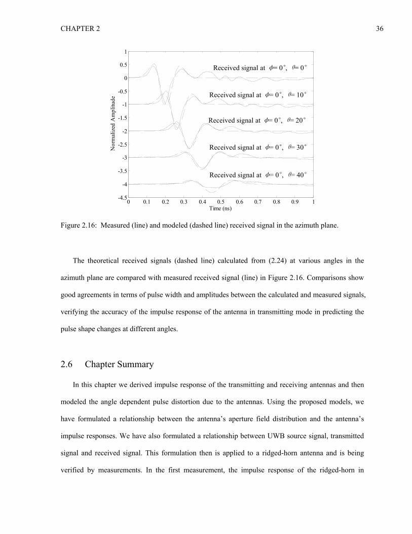
CHAPTER 2 36

The theoretical received signals (dashed line) calculated from (2.24) at various angles in the

azimuth plane are compared with measured received signal (line) in Figure 2.16. Comparisons show

good agreements in terms of pulse width and amplitudes between the calculated and measured signals,

verifying the accuracy of the impulse response of the antenna in transmitting mode in predicting the

pulse shape changes at different angles.

2.6 Chapter Summary

In this chapter we derived impulse response of the transmitting and receiving antennas and then

modeled the angle dependent pulse distortion due to the antennas. Using the proposed models, we

have formulated a relationship between the antenna’s aperture field distribution and the antenna’s

impulse responses. We have also formulated a relationship between UWB source signal, transmitted

signal and received signal. This formulation then is applied to a ridged-horn antenna and is being

verified by measurements. In the first measurement, the impulse response of the ridged-horn in

0 0.1 0.2 0.3 0.4 0.5 0.6 0.7 0.8 0.9 1-4.5

-4

-3.5

-3

-2.5

-2

-1.5

-1

-0.5

0

0.5

1

Time (ns)

Nor

mal

ized

Am

plitu

de






0 0.1 0.2 0.3 0.4 0.5 0.6 0.7 0.8 0.9 1-4.5

-4

-3.5

-3

-2.5

-2

-1.5

-1

-0.5

0

0.5

1

Time (ns)

Nor

mal

ized

Am

plitu

de






Figure 2.16: Measured (line) and modeled (dashed line) received signal in the azimuth plane.

CHAPTER 2 37

receiving mode is compared with direct measurement of received signals. In the second measurement,

the impulse response of the ridged-horn in transmitting mode is verified by transmission and

reception of a UWB signal.

CHAPTER 3 38

CHAPTER 3

ANTENNA NOISE EFFECT ON UWB ANGLE ESTIMATION

3.1 Introduction

In ultra-wideband (UWB) radio systems, the time-difference-of-arrival (TDOA) method [24]−[27]

can be used to find the location of a radar target or a transponder. To do so, we need to estimate the

range and the angle-of-arrival of the incident signal that is either reflected from the radar target, or

transmitted from the transponder. In the TDOA method, the range information is estimated from the

received signal’s time-of-arrival, while the angle-of-arrival information is estimated from the

difference in time-of-arrivals recorded by the receivers of the TDOA array. The TDOA method is

more suitable for UWB than conventional narrowband radio systems. This is because, unlike

narrowband radio systems, UWB transmits and receives signals of short electrical lengths. The

TDOA method can leverage on the inherently short electrical lengths of UWB signals in free-space (6

to 15 cm for a UWB pulse of typical pulse width 0.2 to 0.5 ns) to locate the radar target or

transponder with better accuracy.

The TDOA receiver array, as its name suggests, consists of an array of receivers that estimate the

time-of-arrivals of the received signal, and then feed the time-of-arrival information to the TDOA

processor. To find the range, the TDOA processor calculates the average time-of-arrival from the

receivers, and then calculates the range by considering the absolute delay of the signal (from a

reference time) and the speed of light. To estimate the angle-of-arrival, the TDOA processor finds the

relative difference in the time-of-arrivals and calculates the angle by considering these differences

CHAPTER 3 39

and the locations of the receivers. However, in our initial measurements, the TDOA receiver can only

achieve limited accuracy. The limitation in accuracy is attributed to low signal-to-noise ratios (SNR)

of the received signal. Low SNR compromises the accuracy of the time-of-arrival, which leads to

inaccuracies in estimating the angle-of-arrival, since the angle is calculated from the time-of-arrival.

In this chapter, we propose a model that predicts the TDOA accuracy. The proposed model

considers several factors such as the incident signal, the antenna noise [10] and signal distortions due

to the receiving antennas. It models the TDOA accuracy as a probability density function. The root

mean square of the probability density functions are then verified by experiments. In Sections 3.2 and

3.3, we derive the time-of-arrival accuracy of the received signal and express it as probability density

function. In Section 3.4, we derive the angle-of-arrival accuracy based on the result in Section 3.3. In

Section 3.5, we experimentally verify the time-of-arrival derivations in Sections 3.2 and 3.3. Lastly,

in Sections 3.6 and 3.7, we verify the angle-of-arrival derivations in Section 3.4 by numerical

simulation and experiments.

3.2 Time-of-Arrival Estimation of UWB Signals at Boresight

In this section, we will derive the probability density function for the estimated time-of-arrival of

UWB signals in boresight. Here, we will first describe the UWB cross-correlation receiver and show

how it is used in estimating the time-of-arrival of a received signal. Then, after stating the

assumptions we make on the received signal, we will derive the probability density function.

Figure 3.1 shows the stored reference (SR) cross-correlation receiver [67] that is used to estimate

the UWB signal’s time-of-arrival. Let a UWB signal, e (t), be incident on the receiving antenna from

boresight. Because the receiving antenna does not distort the signal that arrives in boresight direction,

the received signal appears as r (t − τ0), which has the same shape as the incident signal, e (t).

However, the received signal is corrupted by antenna noise n (t) [14]. The antenna noise corrupted

signal, r (t − τ0) + n (t), is cross-correlated with a reference signal, r0 (t − τ), which is generated by the

CHAPTER 3 40

receiver. In this section, we assume that the shape of r (t − τ0) is known and it is used as the reference

signal of the cross-correlator circuit. The received signal’s time-of-arrival, however, is still unknown,

and will be estimated by the receiver.

( ) ( ) ( ) ( )0 00

T

R r t n t r t dtτ τ τ⎡ ⎤= − + ⋅ −⎣ ⎦∫

( )0

...T

dt∫Time-Integration Circuit:

( )0r t τ−Reference Signal:( ) ( )0r t n tτ− +

Received Signal:Multiplication Circuit:

( )0 maxˆ Rτ τ=Decision Circuit:

( ) ( ) ( ) ( )0 00

T

R r t n t r t dtτ τ τ⎡ ⎤= − + ⋅ −⎣ ⎦∫

( )0

...T


( )0

...T


( )0r t τ−Reference Signal:

( )0r t τ−Reference Signal:

( )0r t τ−Reference Signal:( ) ( )0r t n tτ− +

Received Signal:

( ) ( )0r t n tτ− +Received Signal:

Multiplication Circuit:Multiplication Circuit:




Figure 3.1: Schematic of a stored reference cross-correlation receiver estimating the time-of-arrival of

a received signal.

As shown in Figure 3.1, the cross-correlation receiver consists of a multiplication circuit, a time

integration circuit, a reference signal generator circuit and a decision circuit. The multiplication

circuit can be implemented with a diode mixer or a Gilbert cell multiplier. The time integration circuit

can be implemented by low-pass filters. The reference signal generator circuit can be implemented by

a pulse-forming network [59]. The pulse forming network is triggered by a step or clock signal whose

delay, τ, can be controlled. The decision circuit is used to estimate the time-of-arrival of the received

signal. To do so, it collects the cross-correlated values, R (τ = τi), of the received and reference signals

once every pulse repetition interval (PRI) and stores them. τi refers to the reference signal’s delay, τ,

at the i-th interval. At every PRI, τi is increased with a time resolution of Δt s from 0 s to T s. Because

of the gradual increment of τi, after T / Δt number of PRIs, a cross-correlation signal R (τ) will be

CHAPTER 3 41

formed. Once a complete set of R (τ) is known, the decision circuit makes a decision that the

estimated time-of-arrival lies at the instance of maximum cross-correlation. This process is then

repeated to find the next time-or-arrival.

As mentioned earlier, the signal present at the cross-correlator input is an antenna noise corrupted

signal. In the following analysis, it is assumed that the antenna noise behaves as an additive white

Gaussian noise (AWGN), with mean noise power per unit bandwidth of N0. N0 is related to the

antenna temperature, Tant [14], as N0 = kB TB ant , where kBB is the Boltzmann’s constant. The value of N0

can be obtained from n (t) [10], [14] as

( ) 2 20

10

T T t

ii

t tN n t dt tT T

Δ

=

Δ Δ= ≅ ⋅ Δ n∑∫ (3.1)

where n (t) is the measured antenna noise signal, Δt is the time resolution and T is the time-interval of

measured antenna noise signal, n (t). In the following analysis, it is assumed that the signal-to-noise

ratio is large, i.e. Eb / N0 >> 1 [10], where Eb is defined as the energy of the received UWB signal in

one PRI,

( ) 2 20

10

T T t

bi

E r t dt tτ=

= − ≅ Δ ir∑∫ (3.2)

Reference [10] has shown that, in general, the probability density function for the estimated time-

of-arrival of a received signal, τ , based on the stored-reference cross-correlation receiver shown in

Figure 3.1, is

00 2ˆ ~ ,

b s

NNE

τ τβ

⎛⎜⎝ ⎠

⎞⎟ (3.3)

CHAPTER 3 42

where τ0 is the true time-of-arrival, N0 is the antenna noise power and Eb is the energy of the received

pulse within one PRI. βs is the received signal’s second moment [7] defined as

( ) ( )2

22b s

dE r t rdt

β∞

−∞⋅ = ⋅∫ t dt (3.4)

Hence, from the probability density function of (3.3), the root mean square error (standard

deviation) of the estimated time-of-arrival of UWB signal is 01

s b

NEβ

.

3.3 Time-of-Arrival Estimation of UWB Signals at Off-boresight

y

θ( )e t

d

x0

cross correlation( ) ( )0 ,r t n tτ θ− +

( )0r t τ−

max. τ

y

θ( )e t

d

x0

cross correlation( ) ( )0 ,r t n tτ θ− +

( )0r t τ−

max. τ

Figure 3.2: A UWB cross-correlation receiver.

In this section, we will derive the probability density function of the estimated time-of-arrival of

UWB signals at off-boresight angles. The receiver used to estimate the time-of-arrival is the same

cross-correlation receiver, as shown in Figure 3.2. Let the receiving antenna be the double-ridged

horn by RCM Ltd. (model MDRH-1018) shown in Figure 2.2. The azimuth plane impulse response of

the antenna in receiving mode can be derived as

CHAPTER 3 43

( ) 12, , 0 cossin sin 2 2r

k ctf t u t u tατπθ φθ α θ

ατ⎡ ⎤⎛ ⎞ ⎛⎛ ⎞= ° = ⋅ + − −⎜ ⎟ ⎜ ⎟ ⎜⎞⎟⎢ ⎥⎝ ⎠ ⎝ ⎠ ⎝ ⎠⎣ ⎦

(3.5)

where u (t) is a unit step function, k is an proportionality constant, τα = α sin θ / c and α is the width of

the ridged-horn aperture. e (t), the incident UWB signal, has been defined in (2.15) as a second

derivative Gaussian pulse with τ = 60 ps. The received signal is expressed as e

( ) ( ) ( ) ( ) ( ) (0 , , 0 ,n rr t e t )0f t n t r tτ θ φ τ θ= − ⊗ = ° + = − + n t (3.6)

Based on the analysis provided in [10], the likelihood function of estimated time-of-arrival of the

signal (3.6), when received with a stored reference cross-correlation receiver, is

( ) ( ) ( ) ( ) ( )00 0

1exp exp ,T

nP r t r t dt vN

wτ τ τ θ⎡ ⎤

τ⎡ ⎤≅ − =⎢ ⎥ +⎣ ⎦⎣ ⎦

∫ (3.7)

where

( ) ( ) ( ) ( )0 00 0

1, ,T

rv e t f t r tN

τ θ τ θ τ⎡ ⎤= − ⊗ ⋅ −⎣ ⎦∫ dt (3.8)

( ) ( ) ( )00 0

1 T

w n t r tN

τ = ∫ dtτ− (3.9)

and r0 (t) is the reference signal of the cross-correlation receiver. r0 (t) is chosen to have the same

shape as the received UWB signal at boresight direction (φ = θ = 0°),

( ) ( ) ( )0 ,rr t e t f t φ θ 0= ⊗ = = ° (3.10)

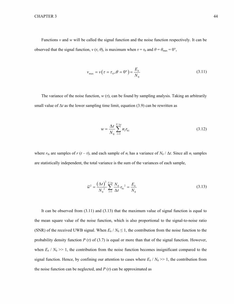
CHAPTER 3 44

Functions v and w will be called the signal function and the noise function respectively. It can be

observed that the signal function, v (τ, θ), is maximum when τ = τ0 and θ = θmax = 0°,

( )max 00

, 0 bEv vN

τ τ θ= = = ° = (3.11)

The variance of the noise function, w (τ), can be found by sampling analysis. Taking an arbitrarily

small value of Δt as the lower sampling time limit, equation (3.9) can be rewritten as

010

T t

i ii

twN

Δ

=

Δ= ∑ n r (3.12)

where r0i are samples of r (t – τ), and each sample of ni has a variance of N0 / Δt. Since all ni samples

are statistically independent, the total variance is the sum of the variances of each sample,

( )22 0

0210 0

T tb

ii

t Nw rN t

Δ

=

Δ=

Δ∑ 2 EN

= (3.13)

It can be observed from (3.11) and (3.13) that the maximum value of signal function is equal to

the mean square value of the noise function, which is also proportional to the signal-to-noise ratio

(SNR) of the received UWB signal. When Eb / N0 ≤ 1, the contribution from the noise function to the

probability density function P (τ) of (3.7) is equal or more than that of the signal function. However,

when Eb / N0 >> 1, the contribution from the noise function becomes insignificant compared to the

signal function. Hence, by confining our attention to cases where Eb / N0 >> 1, the contribution from

the noise function can be neglected, and P (τ) can be approximated as

CHAPTER 3 45

( ) ( ) ( ) ( ) ( )0 00 0

1exp , exp ,T

rP v e t f t r t dN

τ τ θ τ θ τ t⎧ ⎫⎪ ⎪⎡ ⎤ ⎡ ⎤≅ = − ⊗ ⋅ −⎨ ⎬⎣ ⎦ ⎣ ⎦⎪ ⎪⎩ ⎭

∫ (3.14)

To further simplify the likelihood function, let v (τ, θ) in (3.14) be expanded about τ0 by Taylor’s

theorem, resulting in

( ) ( ) ( )( ) ( )( ) ( )

22 02

0 20 0

1 1exp 1 ... exp2 2 2

bs

b s

EP

N N Eθ τ

τ β θ τ τθ β θτ⎧ ⎫⎧ ⎫ −⎪ ⎪⎡ ⎤≅ − − + ∝⎨ ⎬ ⎨⎢ ⎥ ⎬

⎡ ⎤⎣ ⎦⎩ ⎭ ⎪ ⎪⎣ ⎦⎩ ⎭ (3.15)

where

( ) ( ) ( ) ( )0 00

,T

b rE e t f t r tθ τ θ⎡ ⎤= − ⊗ ⋅ −⎣ ⎦∫ dtτ (3.16)

( ) ( ) ( ) ( ) ( )2

20 02

0

,T

b s rdE e t f t r t dtdt

θ β θ τ θ τ⎡ ⎤ ⎡ ⎤= − ⊗ ⋅ −⎣ ⎦ ⎣ ⎦∫ (3.17)

Equation (3.15) shows that the estimated time-of-arrival is a Gaussian probability density

function

( ) ( )0

0 2ˆ ~ ,b s

NNE

τ τθ β θ

⎡ ⎤⎢ ⎥⎢ ⎥⎣ ⎦

(3.18)

Hence, from the variance expression of (3.18), we can derive the root mean square error of the

estimated time-of-arrival of UWB signal as

CHAPTER 3 46

( ) ( ) ( )01

s b

NEτσ θ

β θ θ= (3.19)

3.4 Angle-of-Arrival Estimation of UWB TDOA Receivers

In this section, we will derive the probability density function of the estimated angle-of-arrival by

the UWB TDOA receiver array. To do that, we will first describe the TDOA array and how the

TDOA processor estimates the angle-of-arrival. Then, the TDOA array will be modeled to derive the

angle-of-arrival accuracy.

y

θ

( )e t

d d

2s

−

x2s

+

0

cross correlation

cross correlation

( ) ( )2 2 2,r t n tτ θ− +

( )0r t τ−

max.

max. 2τ

( ) ( )1 1 1,r t n tτ θ− +1τ

y

θ

( )e t

d d

2s

−

x2s

+

0

cross correlation

cross correlation

( ) ( )2 2 2,r t n tτ θ− +

( )0r t τ−

max.

max. 2τ

( ) ( )1 1 1,r t n tτ θ− +1τ

Figure 3.3: A UWB Time-difference-of-arrival (TDOA) receiver array.

Figure 3.3 shows a UWB TDOA array of two receivers. Each receiver captures the incident

signal, e (t), with a ridged-horn. The ridged-horn is connected to a stored-reference cross-correlator

receiver that has been described in Section 3.2. The ridged-horn of the left receiver (Figure 3.3) is

labeled as RH1, while the ridged-horn of the right receiver (Figure 3.3) is labeled as RH2. Both RH1

and RH2 have the same aperture length of d = 0.236 m. Modeling of this TDOA receiver will only be

done for the azimuth plane.

Let the received UWB signals of RH1 and RH2 be r1 (t – τ1, θ) and r2 (t – τ2, θ) respectively. θ is

the angle-of-arrival of the transmitted signal incident on the TDOA receiver; while τ1 and τ2 are the

CHAPTER 3 47

true time-of-arrivals of the received UWB signals from receivers RH1 and RH2. In the receivers, r1

and r2 are cross-correlated with the reference signal r0 (3.10). The process of estimating the time-of-

arrivals of r1 and r2 is similar to that described in Section 3.2. The impulse responses of the antennas

RH1 and RH2 in receiving mode are fr1 (t, θ, φ = 0°) and fr2 (t, θ, φ = 0°) respectively, where

( ) ( ) ( )121

sin sin1 sin, , 0 cossin sin 2 2 2r

s d s dc sf t t u t u td c c c

θ θπ θθ φθ θ

⎧ ⎫⎡ ⎤ ⎡ ⎤+ −⎡ ⎤ ⎪ ⎪⎛ ⎞= ° = − ⋅ − − −⎨ ⎬⎢ ⎥ ⎢ ⎥⎜ ⎟⎢ ⎥⎝ ⎠⎣ ⎦ ⎪ ⎪⎣ ⎦ ⎣ ⎦⎩ ⎭(3.20)

( ) ( ) ( )122

sin sin1 sin, , 0 cossin sin 2 2 2r

s d s dc sf t t u t u td c c c

θ θπ θθ φθ θ

⎧ ⎫⎡ ⎤ ⎡ ⎤− +⎡ ⎤ ⎪ ⎪⎛ ⎞= ° = + ⋅ + − −⎨ ⎬⎢ ⎥ ⎢ ⎥⎜ ⎟⎢ ⎥⎝ ⎠⎣ ⎦ ⎪ ⎪⎣ ⎦ ⎣ ⎦⎩ ⎭ (3.21)

Let 1τ and 2τ be the estimated time-of-arrivals of the received signals from receivers RH1 and

RH2 respectively. Applying the same analysis that derived (3.18) in Section 3.3, we can derive the

probability density function of 1τ and 2τ as

( ) ( )1

1 1 2ˆ ~ ,b

NNE

τ τθ β θ

⎡ ⎤⎢ ⎥⎢ ⎥⎣ ⎦

(3.22)

( ) ( )2

2 2 2ˆ ~ ,b

NNE

τ τθ β θ

⎡ ⎤⎢ ⎥⎢ ⎥⎣ ⎦

(3.23)

It can be observed from the relative positions of the receivers RH1 and RH2, in Figure 3.3, that

the estimated angle-of-arrival, , is related toθ 1τ and 2τ as

( 2 1ˆ ˆ ˆsin c

s)θ τ τ= − (3.24)

CHAPTER 3 48

where c is the speed of light in free space and s is the separation between the antennas. Substituting

the probability density functions of 1τ and 2τ into (3.24), the probability density function of sin can

be derived as

θ

( )( ) ( )

21 2

2 2ˆsin ~ sin ,

c N NN

s Eθ θ

β θ θ⎡ ⎤+⎢⎢ ⎥⎣ ⎦

⎥ (3.25)

However, for (3.25) to be valid, values assumed by sin must be contained within [-1, 1]. Values

beyond [-1, 1] have to be discarded because they do not translate into a valid θ value. Hence, the

probability density function of (3.25) has to be doubly-truncated [68] at [-1, 1] to

θ

ˆ

( ) ( )( )1

1

ˆ0 , sinˆsin

ˆ ˆsin , 1 sin 1ˆ ˆsin sin

ˆ0 , 1 sin

DTN

PP

P d

θ

θθ

θ θ

θ−

⎧ 1

θ

−∞ ≤ ≤ −⎪⎪⎪= −⎨⎪⎪⎪

≤ ≤ +

+ ≤ ≤ +⎩

∫∞

(3.26)

Double truncation also results in inaccurate angle-of-arrival predictions at the angles near ±90°.

This inaccuracy is acceptable since most angle-of-arrival estimations are done within the 3-dB

beamwidth of the receiver antennas, which is far away from ±90°. Probability density function of

can be calculated from probability density function of doubly-truncated sin by a one-to-one

mapping method of a random variable function [69] as

θ

θ

( )2

ˆ0 ,

ˆ ˆcos 1 sin sinˆ ˆexp , 90 9022

ˆ0 , 90

DTNPk

θ

θ θ θθ θσπσ

θ

⎧ 90−∞ ≤ ≤ − °⎪

⎡ ⎤⎪ ⎛ ⎞−⎪ ⎢ ⎥= − − ° ≤ ≤ +⎜ ⎟⎨ ⎜ ⎟⎢ ⎥⎝ ⎠⎪ ⎣ ⎦⎪

°

+ ° ≤ ≤ +∞⎪⎩

(3.27)

CHAPTER 3 49

where θ is only defined within [−90°, 90°], and

( )21

1

11

ˆ1 1 sin sinˆ ˆsin sin exp sin22

k P d dθ θ ˆθ θ θσπσ−

−

⎡ ⎤⎛ ⎞−⎢= = − ⎜ ⎟⎜ ⎟⎢ ⎥⎝ ⎠⎣ ⎦∫ ∫ ⎥ (3.28)

( )( ) ( )

21 22

2 2

c N Ns E

σβ θ θ

+= (3.29)

The theoretical variance of can be expressed as θ

( )290 22

ˆ ˆ90

ˆ ˆcos 1 sin sinˆ ˆexp22

dkθ θ

θ θ θσ θ μ θσπσ−

⎡ ⎤⎛ ⎞−⎢ ⎥= − − ⎜ ⎟⎜ ⎟⎢ ⎥⎝ ⎠⎣ ⎦∫ (3.30)

where

290

ˆ90

ˆ ˆ ˆcos 1 sin sin ˆexp22

dkθ

θ θ θ θμ θσπσ−

⎡ ⎤⎛ ⎞−⎢ ⎥= − ⎜ ⎟⎜ ⎟⎢ ⎥⎝ ⎠⎣ ⎦∫ (3.31)

Hence, the theoretical root mean square error (standard deviation) of angle-of-arrival, , for an

arbitrary SNR can be calculated numerically from (3.30).

θ

3.5 Verification of Time-of-Arrival Derivations

In Sections 3.2 and 3.3, the time-of-arrival accuracy has been derived for the case of a radiated

UWB signal incident on a ridged-horn antenna. The derived accuracy, expressed in root-mean-square

error, will be experimentally verified in this section. In the experiment, a UWB source is placed at

CHAPTER 3 50

far-field distance and radiates a train of UWB pulses. The amplitude of the radiated signal can be

adjusted, by adding attenuators, so that different signal-to-noise ratios (SNR) can be achieved at the

receiver. The radiated UWB signal is received by a ridged-horn antenna, and measured with a 40

GS/s sampling oscilloscope. During the measurement, no averaging is applied to the measured signal

in the sampling oscilloscope. The receiving ridged-horn antenna is placed on a turn-table, which

rotates in the azimuth plane from θ = -20° to 20°, at 1° intervals. In each interval, 50 samples of

received signals are collected. The measurements are done at both antennas RH1 and RH2.

Furthermore, the collection of received signals is repeated for three different UWB source amplitudes.

During the measurements, it is observed that receiving antennas RH1 and RH2 introduce different

power levels of antenna noise to the received signal. Hence, by using both the antennas to receive

radiated UWB signal at three different power levels, the received signal data for six cases of signal-

to-noise ratios (SNR) can be analyzed.

0 0.2 0.4 0.6 0.8 1 1.2 1.4 1.6 1.8 2-25

-20

-15

-10

-5

0

5

10

Time (ns)

Am

plitu

de (m

V)

Received Signal from RH1


0 0.2 0.4 0.6 0.8 1 1.2 1.4 1.6 1.8 2-25

-20

-15

-10

-5

0

5

10

Time (ns)

Am

plitu

de (m

V)



Figure 3.4: A sample of measured received signal with antennas RH1 and RH2.

CHAPTER 3 51

Figure 3.4 shows a sample of the measured signal with antennas RH1 and RH2 at boresight. It

can be seen from both traces that the received signal is corrupted with thermal noise, making it

difficult to judge the true time-of-arrival. These measured signals are cross-correlated with the

reference signal r0 (3.10), and the instance of maximum cross-correlation is recorded as estimated

time-of-arrivals. From the measured samples, the root mean square error can be found and compared

with the derived root mean square error in (3.3) and (3.18).

0 0.5 1 1.5 2-12

-10

-8

-6

-4

-2

0

2

Time (ns)

Am

plitu

de (m

V)

received e1 pulse

received e2 pulse

received e3 pulse

0 0.5 1 1.5 2-12

-10

-8

-6

-4

-2

0

2

Time (ns)

Am

plitu

de (m

V)

received e1 pulse

received e2 pulse

received e3 pulse

Figure 3.5: Measured received signal with antennas RH1 (dotted line) and RH2 (dashed line)

compared to the modeled received signal (line) in three power levels.

To find the value of Eb (θ), we need to measure the received signal without noise corruption. To

do that, the noise corrupted received signal is averaged 4096 times so that antenna noise corruption is

suppressed. The dotted and dashed lines in Figure 3.5 are the measured received signals of three

power levels – labeled as e1, e2 and e3. The dotted line corresponds to antenna RH1 and the dashed

line corresponds to antenna RH2. Let the energies of an e1, e2 and e3 pulse be Eb1, Eb2 and Eb3

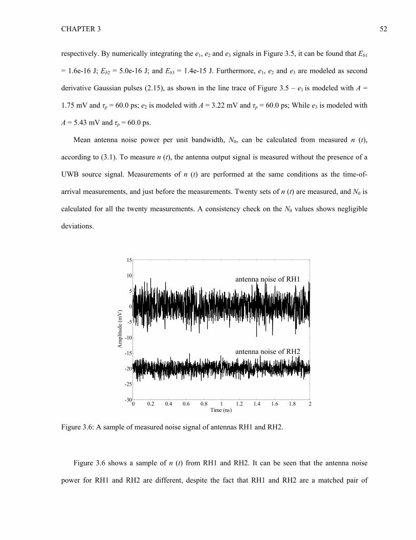
CHAPTER 3 52

respectively. By numerically integrating the e1, e2 and e3 signals in Figure 3.5, it can be found that Eb1

= 1.6e-16 J; Eb2 = 5.0e-16 J; and Eb3 = 1.4e-15 J. Furthermore, e1, e2 and e3 are modeled as second

derivative Gaussian pulses (2.15), as shown in the line trace of Figure 3.5 – e1 is modeled with A =

1.75 mV and τp = 60.0 ps; e2 is modeled with A = 3.22 mV and τp = 60.0 ps; While e3 is modeled with

A = 5.43 mV and τp = 60.0 ps.

Mean antenna noise power per unit bandwidth, N0, can be calculated from measured n (t),

according to (3.1). To measure n (t), the antenna output signal is measured without the presence of a

UWB source signal. Measurements of n (t) are performed at the same conditions as the time-of-

arrival measurements, and just before the measurements. Twenty sets of n (t) are measured, and N0 is

calculated for all the twenty measurements. A consistency check on the N0 values shows negligible

deviations.

0 0.2 0.4 0.6 0.8 1 1.2 1.4 1.6 1.8 2-30

-25

-20

-15

-10

-5

0

5

10

15

Time (ns)

Am

plitu

de (m

V)

antenna noise of RH1


0 0.2 0.4 0.6 0.8 1 1.2 1.4 1.6 1.8 2-30

-25

-20

-15

-10

-5

0

5

10

15

Time (ns)

Am

plitu

de (m

V)



Figure 3.6: A sample of measured noise signal of antennas RH1 and RH2.

Figure 3.6 shows a sample of n (t) from RH1 and RH2. It can be seen that the antenna noise

power for RH1 and RH2 are different, despite the fact that RH1 and RH2 are a matched pair of

CHAPTER 3 53

ridged-horns. This difference is attributed to errors in fabrication and mechanical tolerances of the

ridged-horn. The measured value of antenna noise for RH1 is N1 = 12.3e-18 J and RH2 is N2 = 2.7e-

18 J. From (3.17), βs2 value can be numerically calculated for all the relevant angles. From the

measured values of Eb1 (θ), Eb2 (θ), Eb3 (θ), N1 and N2, the theoretical standard deviation (root mean

square error) can be calculated, and compared with the measured root mean square error. The

comparisons at boresight, ±10° and ±20° are shown in Tables 3.1, 3.2 and 3.3 respectively.

No. SNR Eb / N0

(dB) s.d. (theoretical)

s.d. (measured)

1. Eb1 / N1 11.1 7.44 ps 10.857 ps 2. Eb 2 / N1 16.1 4.21 ps 4.591 ps 3. Eb 1 / N2 17.7 3.49 ps 6.083 ps 4. Eb 3 / N1 21.3 2.52 ps 1.612 ps 5. Eb 2 / N2 22.7 1.97 ps 2.057 ps 6. Eb 3 / N2 27.1 1.179 ps 1.535 ps

Table 3.1: Theoretical and experimental time-of-arrival standard deviation at boresight for six cases

of SNR.

No. SNR Eb / N0


s.d. (-ve) measured

s.d. (+ve) measured

1. Eb1 / N1 10.1 8.58 ps 6.00 ps 5.45 ps 2. Eb2 / N1 15.4 4.66 ps 14.29 ps 5.82 ps 3. Eb1 / N2 16.7 4.02 ps 4.97 ps 3.30 ps 4. Eb3 / N1 19.9 2.76 ps 2.82 ps 2.20 ps 5. Eb2 / N2 22.0 2.18 ps 5.27 ps 3.06 ps 6. Eb3 / N2 26.5 1.29 ps 1.72 ps 1.07 ps

Table 3.2: Theoretical and experimental time-of-arrival standard deviation at ± 10° for six cases of

SNR.

CHAPTER 3 54

No SNR Eb / N0


s.d. (-ve) measured

s.d. (+ve) measured

1. Eb1 / N1 7.9 11.59 ps 6.49 ps 12.57 ps 2. Eb2 / N1 13.2 6.29 ps 8.68 ps 9.14 ps 3. Eb1 / N2 14.5 5.43 ps 3.43 ps 4.22 ps 4. Eb3 / N1 17.8 3.73 ps 3.14 ps 3.57 ps 5. Eb2 / N2 19.8 2.95 ps 2.39 ps 5.64 ps 6. Eb3 / N2 24.4 1.75 ps 1.62 ps 1.85 ps

Table 3.3: Theoretical and experimental time-of-arrival standard deviation at ± 20° for six cases of

Comparison between theoretical and measured standard deviations shows that there is good

agreement between the two values.

3.6 Numerical Simulation of Angle-of-Arrival

In this section, the theoretical standard deviation (root mean square error) calculated from (3.30)

will be verified by simulation. To make sure that the simulated values of angle-of-arrival accuracy

can be effectively compared with the theoretical and measured values, the simulation need to be done

in conditions that are similar to the measurement. In the measurement, received signals in three power

levels are measured. The energies of the received UWB signals are: Eb1 = 1.6e−16 J; Eb2 = 5.0e−16 J;

and Eb3 = 1.4e−15 J. As mentioned in the last section, the measured antenna noise power per unit

bandwidth of RH1 and RH2 are N1 = 12.3e−18 J and RH2 is N2 = 2.7e−18 J respectively.

Based on these values, the theoretical standard deviation (3.30) has been calculated, and

presented in Figure 3.7. In Figure 3.7, Case 1 refers to the situation where the received UWB signal

has the energy of Eb1 in a pulse repetition interval (PRI); Case 2 refers to the situation where the

received UWB signal has the energy of Eb2 in a PRI; and Case 3 refers to the situation where the

received UWB signal has the energy of Eb3 in a PRI. For all the Cases 1-3, the receiving antennas are

RH1 and RH2 with antenna noise of N1 and N2 respectively.

CHAPTER 3 55

-20 -15 -10 -5 0 5 10 15 200

0.1

0.2

0.3

0.4

0.5

0.6

0.7

0.8

0.9

1

Angle of arrival (AOA) (degrees)

Stan

dard

Dev

iatio

n of

AO

A e

stim

atio

n (d

egre

es)

Case 1

Case 2

Case 3

Figure 3.7: Theoretical standard deviations of estimated angle-of-arrival (AOA) for three cases of

signal-to-noise ratio (SNR).

g (t – τ0) n (t)

g (t – τ)1τ

2τ

h1 (t)

h2 (t)

Eb

Eb

N1

N2

( )0

...T

dt∫

( )0

...T

dt∫

τmax.

τmax.

g (t – τ0) n (t)

g (t – τ)1τ

2τ

h1 (t)h1 (t)

h2 (t)h2 (t)

EbEb

EbEb

N1N1

N2N2

( )0

...T

dt∫ ( )0

...T

dt∫

( )0

...T

dt∫ ( )0

...T

dt∫

τmax.τmax.

τmax.τmax.

Figure 3.8: Schematic of simulation process to verify the TDOA receiver’s angle-of-arrival accuracy.

The simulation is performed in MATLAB – a mathematical software. In the simulation, the

received UWB signals are generated by convolution of (2.15) and (3.5), and are scaled according to

the energy levels of Eb1, Eb2 and Eb3. The antenna noise is generated by an existing AWGN noise

CHAPTER 3 56

signal generator in MATLAB. The antenna noise power is scaled according to N1 and N2, and then

added to the received UWB signal to simulate the noise corrupted received signal. This signal is then

cross-correlated with a 1 V amplitude reference signal, which is generated as defined in (3.10). The

instances of maximum cross-correlation for both receivers are found, and substituted into equation

(3.24) to calculate the estimated angle-of-arrival for one sample of data. Diagrammatically, the

simulation process is shown in Figure 3.8.

For every angle, 200 samples of angle-of-arrival data are collected based on the simulation as

described by Figure 3.8. The standard deviations from the simulations are tabulated and shown in

Figure 3.9.

-20 -15 -10 -5 0 5 10 15 200

0.5

1

1.5

2

2.5

3

3.5

4


Sta

ndar

d de

viat

ion

of A

OA

est

imat

ion

(deg

rees

)

Case 1

Case 2

Case 3

-20 -15 -10 -5 0 5 10 15 200

0.5

1

1.5

2

2.5

3

3.5

4


Sta

ndar

d de

viat

ion

of A

OA

est

imat

ion

(deg

rees

)

Case 1

Case 2

Case 3

Figure 3.9: Simulated standard deviations of estimated angle-of-arrival (AOA) for three cases of

signal-to-noise ratio (SNR).

CHAPTER 3 57

3.7 Measurement of Angle-of-Arrival

In this section, the theoretical standard deviation (root mean square error) calculated from (3.30)

will be verified by measurements. Figure 3.10 shows the measurement setup. In the measurement, the

UWB TDOA receiver array, consisting of two double ridged-horns by RCM Ltd. (model MDRH-

1018), are placed on a turn-table. The ridge-horns RH1 and RH2 are placed at a distance s = 0.263 m

apart, with their aperture length d = 0.236 m. The turn-table is rotated, at 1° intervals, from −20° to

20°. The time domain signals are measured by a time-synchronized 40 GS/s sampling oscilloscope.

To synchronize the pulse generator at the transmitter and the sampling oscilloscope, a 6.0 m coaxial

cable is connected from the trigger signal of the pulse generator to the trigger input of the sampling

oscilloscope.

Woo

d su

ppor

t

UWB pulse sourceW

ood

supp

ortReceiver antennas

Turn

-tabl

e

equallengthwires

samplingoscilloscope

synchronization

3 m

1.5 m 1.5 m

Woo

d su

ppor

t

UWB pulse sourceW

ood

supp

ortReceiver antennas

Turn

-tabl

e

equallengthwires

samplingoscilloscope

synchronization

3 m

1.5 m 1.5 m

Figure 3.10: Angle-of-Arrival measurement setup.

Figure 3.11 shows a photograph of the setup during one of the angle-of-arrival measurements.

The incident UWB pulse is radiated by an antenna placed at far-field distance. 50 samples of signals

are measured (at both receivers) for every 1° rotation. The wooden turn-table seen in Figure 3.11 is

constructed by bolting two circular boards together in alignment. To achieve measurements of 1°

CHAPTER 3 58

accuracy, a Vernier scale is used – the lower circular board is marked at 10° intervals, while the upper

circular board is marked at 11° intervals. The antennas are directly connected to the sampling

oscilloscope with two equal length coaxial cables, as shown in Figure 3.11. The measured signals are

then cross-correlated with the reference signal to obtain samples of measured angle-of-arrivals.

Figure 3.11: Picture of Angle-of-Arrival measurement setup.

A sample of measured waveform is shown in Figure 3.12, where received signals from antennas 1

and 2 are plotted with their respective cross-correlation outputs for Case 2 SNR at θ = +10°. For the

case in Figure 3.12, = 0.85 ns and = 1.03 ns, giving an angle-of-arrival reading of +11.8°, which

is slightly off from θ = +10°.

1τ 2τ

CHAPTER 3 59

0 0.5 1 1.5 2-70

-60

-50

-40

-30

-20

-10

0

10

20

Time (ns)

Am

plitu

de (m

V)

RH1 output

RH1 correlator output

RH2 output


0 0.5 1 1.5 2-70

-60

-50

-40

-30

-20

-10

0

10

20

Time (ns)

Am

plitu

de (m

V)

RH1 output


RH2 output


Figure 3.12: Measured received signals and correlator outputs for antennas RH1 and RH2 at θ =

+10°, Case 2 SNR.

-30 -20 -10 0 10 20 300

5

10

15

20

25

30

Estimated Angle of Arrival (AOA) (degrees)

Num

ber o

f rea

ding

s

10°

15° 20°

5°

0°-5°

-10°

-15°

-20°

-30 -20 -10 0 10 20 300

5

10

15

20

25

30

Estimated Angle of Arrival (AOA) (degrees)

Num

ber o

f rea

ding

s

10°

15° 20°

5°

0°-5°

-10°

-15°

-20°

Figure 3.13: Distribution of measured Angle-of-Arrival (AOA) for θ = 10° (line) and other angles

(dotted lines).

CHAPTER 3 60

Figure 3.13 shows the distribution of measured angle versus true angle for experiments based on

Case 2. Figure 3.13 shows that the measured angles follow the Gaussian-like distribution centered at

their true angles. At boresight (Figure 3.13 – ‘0°’), the Gaussian-like distribution has the smallest

standard deviation. As the target angle moves away from boresight, the standard deviation increases

as predicted. The solid line in Figure 3.13 shows the measured angles at a true angle of +10°. The

measurements, however, register two wrong readings: −9.8° and +20°. This error occurs randomly

when the cross-correlation of reference signal with thermal noise registers a higher value than the

cross-correlation of reference and received signal. The occurrences of such errors, despite not being

considered in the modeling, exist and are major sources of errors in simulation and measurement.

Table 3.4 shows the mean and standard deviation of measured angles. The measured mean

deviates slightly from the true angle because of errors in steering the turn-table. The increasing trend

of standard deviations shows that accuracy of angle estimation errors varies from 0.1° at boresight to

3.0° at ± 20°.

Case 1: Case 2: Case 3: Angle μ1 / ° σ1 / ° μ2 / ° σ2 / ° μ3 / ° σ3 / °

-20 -18.7 3.0 -17.7 3.3 -18.2 2.6 -15 -13.4 2.0 -13.0 2.1 -13.2 1.9 -10 -9.0 1.4 -8.4 2.0 -8.7 1.3 -5 -4.3 0.7 -3.5 0.6 -3.9 0.6 0 1.8 0.8 0.5 0.3 0.1 0.1 5 4.4 1.5 5.2 0.8 4.7 0.7 10 8.9 2.0 11.6 1.8 9.1 1.3 15 14.1 2.7 14.5 2.1 13.9 2.0 20 18.5 3.2 19.9 2.6 18.5 2.7

Table 3.4: Measured mean and standard deviation of angle-of-arrival for the three cases of SNR.

Theoretical, simulated and measured standard deviations are compared in Figure 3.14−16 for

three cases of SNRs. The standard deviation in all cases shows similar values at the angles near

boresight. Figure 3.14 shows that Case 1 theoretical standard deviation ranges from 0.6°−0.9°, while

CHAPTER 3 61

measured standard deviation ranges from 0.5°−3.5°. Figure 3.15 shows that Case 2 theoretical

standard deviation ranges from 0.4°−0.5°, while measured standard deviation ranges from 0.4°−3.3°.

Figure 3.16 shows that Case 3 theoretical standard deviation ranges from 0.3°−0.4°, while measured

standard deviation ranges from 0.3°−2.6°. Although similar trends are observed in measured standard

deviation i.e. the standard deviation increases with decreasing SNR, and increases with increasing θ,

the measured values are higher than the theoretical value.

These differences become evident at off-boresight angles, and could be attributed to several

reasons. Firstly, the proposed model only accounts for the noise contribution at the main peak of the

correlator output. It did not account for effect of combination of noise and signal contributions at

other local maxima besides the main maxima, thus underestimating the standard deviation of angle-

of-arrival error. Next, as θ increases, the ratio Eb (θ) / N0 decreases. This decrease in SNR causes the

higher order terms of the Taylor-expansion of (3.15) to have more significant contribution. Thus, by

truncating the expansion at the 3rd term, the probability density function of time-of-arrival (3.18)

becomes less accurate at larger theta values, which compromises the accuracy of angle-of-arrival.

Thirdly, the probability of w (t) > v (t, θ) in (3.7) increases as the SNR decreases. This results in a

higher number of erroneous time-of-arrival readings during measurements and simulations. This

effect becomes more prominent as θ increases, causing greater deviation from theoretical results at

larger θ values. Lastly, equations (3.20) and (3.21) are approximate models of aperture distribution

functions of a ridged-horn, causing the modeled received signal to be slightly different from measured

received signal at off-boresight angles, as can be seen in [55] and [58]. These differences cause a

slight over-estimation of theoretical cross-correlation values compared with measurement.

CHAPTER 3 62

-20 -15 -10 -5 0 5 10 15 200

0.5

1

1.5

2

2.5

3

3.5

4


Stan

dard

dev

iatio

n of

AO

A e

stim

atio

n (d

egre

es)

Simulated

Measured

Theoretical

Figure 3.14: Theoretical, simulated and measured standard deviations of angle of arrival (AOA)

estimation for Case 1 SNR.

-20 -15 -10 -5 0 5 10 15 200

0.5

1

1.5

2

2.5

3

3.5

4


Stan

dard

dev

iatio

n of

AO

A e

stim

atio

n (d

egre

es)

Simulated

Measured

Theoretical



CHAPTER 3 63

-20 -15 -10 -5 0 5 10 15 200

0.5

1

1.5

2

2.5

3

3.5

4


Stan

dard

dev

iatio

n of

AO

A e

stim

atio

n (d

egre

es)

Simulated

Measured

Theoretical



3.8 Chapter Summary

In this chapter, we have presented a method to derive the accuracy of angle-of-arrival (AOA)

estimation for thermal noise corrupted signal of UWB receiver. The derivation involves expanding

Woodward’s [10] estimation of time-of-arrival to incorporate the antenna pulse shaping effect of

UWB signals. The probability density function of the angle-of-arrival is also derived and its statistical

characteristics compared with simulation and measurements.

CHAPTER 4 64

CHAPTER 4

DESIGN OF ULTRA-WIDEBAND MONOPULSE RECEIVER

4.1 Introduction

Monopulse technique is a radar technique to locate the angular direction of a target by receiving

the incident signal simultaneously with two or more antennas [29]. It is used in existing pulsed and

continuous-wave radars to track targets, providing guidance information and steering commands for

missiles in missile-range instrumentations [30], [31]. Monopulse technique was proposed for ultra-

wideband (UWB) radars [32] by Harmuth et. al.. The monopulse sum and difference patterns were

derived for the case of equally spaced dipoles receiving short, rectangular pulses [32]−[35], and point

antennas receiving Generalised Gaussian UWB Pulses [36]. Furthermore, two methods for finding the

target direction were proposed in [36] – the slope processor and the linear-regression processor. Both

processors’ performances were studied in [36] when the sum and difference signals are corrupted by

additive thermal noise.

In this chapter, a square-feed array [30] of four ridged-horns is considered for UWB monopulse

receiver. Pulse distortion by the ridged-horn array needs to be considered because the array size is

comparable with the electrical length of the incident UWB signal. To model the pulse distortion by

the array, we will define a semi-continuous aperture function for the monopulse array, and then

inverse Fourier transform it in spatial domain to derive the impulse response. A UWB monopulse

receiver is also proposed. Furthermore, the accuracy of the monopulse receiver in estimating the

UWB signal’s angle-of-arrival is derived. The reception accuracy of the monopulse receiver is

CHAPTER 4 65

modelled as a probability density function, and the prediction accuracy of the model is verified with

measured results of angle-of-arrival.

The proposed monopulse receiver is different from the receivers proposed by Harmuth and

Hussain [32]−[36] in the following ways: Firstly, the pulse distortion due to the receiving antennas

was not considered in [32]−[36], but it is considered in this UWB monopulse receiver. Secondly, the

comparator circuit in [32]−[36] was placed after the sliding correlator and variable delay circuit;

while in this UWB monopulse receiver, the comparator circuit is placed directly after the receiving

antennas. This configuration avoids the problem of amplitude and phase mismatches at the sum and

difference channels that may cause performance degradation of the monopulse receiver. Thirdly, to

achieve the time resolution in detecting the signal gradient in the slope and linear-regression

processors [35], [36], a high speed circuit is required to register the received signal amplitudes at

different instances within the pulse width. In the proposed method, the monopulse receiver registers

the cross-correlation output at the pulse repetition frequency, thus reducing the design requirements

of the receiver.

In Section 4.2, we present an analysis to derive the impulse response of the monopulse square-

feed array. In Section 4.3, we present a design of correlator-based UWB monopulse receiver. The

receiver’s output can then be processed by an Amplitude-Comparison monopulse processor [70] to

estimate the angular position of the target. Measurements are presented in Section 4.4 to verify the

impulse response of the monopulse array and the performance of the monopulse receiver. In Section

4.5, we will derive the accuracy of the monopulse receiver in estimating the angle-of-arrival, and

verify it with measurements.

4.2 Impulse Response of Monopulse Square-Feed Array

A monopulse array of four ridged-horns is arranged in a square-feed configuration in the x’y’-

plane, as shown in Figure 4.1. (x’, y’, z’) represents the coordinates of the antenna aperture, while (r,

CHAPTER 4 66

θ, φ) represents the coordinates of the incident pulse, where θ and φ denotes the angles subtending

from z’ and x’-axes respectively. The ridged-horn apertures are labeled as A, B, C and D. All the

ridged-horn apertures have the same dimensions of d1 × d2 and the same aperture field distribution.

The distances between adjacent ridge-horn apertures in the x’ and y’ directions are s1 and s2

respectively. The measured dimensions of the antenna configuration shown in Figure 4.1 are: d1 =

0.236 m, d2 = 0.129 m, s1 = 0.253 m and s2 = 0.145 m.

x’

y’

z’

d1 d1

s1

d2

d2

s2

P (r, θ, φ)

A B

C Dx’

y’

z’

d1d1 d1d1

s1s1

d2

d2

s2

P (r, θ, φ)

A B

C D

Figure 4.1: Monopulse receiver coordinate systems and antenna dimensions.

Σ

Δ

Σ

Δ

Σ

Δ

Σ

Δ

A

B

C

D

sum (A+B)+(C+D)

elevation difference(A+B)−(C+D)

azimuth difference(A−B)+(C−D)

Received signal from antenna: (A+B)

(C+D)

(C−D)

(A−B)

matched load

Σ

Δ

Σ

Δ

Σ

Δ

Σ

Δ

Σ

Δ

Σ

Δ

Σ

Δ

Σ

Δ

A

B

C

D

sum (A+B)+(C+D)

elevation difference(A+B)−(C+D)

azimuth difference(A−B)+(C−D)

Received signal from antenna: (A+B)

(C+D)

(C−D)

(A−B)

matched load Figure 4.2: Monopulse comparator circuit with four 180° hybrid-couplers.

CHAPTER 4 67

To obtain the monopulse sum and difference signals, the antenna apertures are connected to a

comparator circuit [30] consisting of four 180° hybrid-couplers in the manner as shown in Figure 4.2.

The outputs of the comparator are the sum signal, elevation difference signal, and azimuth difference

signal. In Chapter 2, the pulse distortions due to the antennas were modeled as the impulse response

of the antenna in transmitting or receiving mode − ft (t, θ, φ) and fr (t, θ, φ). In this chapter, pulse

distortions of the UWB monopulse array are modeled in a similar manner. To do so, impulse response

of the monopulse array is defined for the sum, elevation difference and azimuth difference arrays.

Let the impulse responses of the monopulse array for sum, elevation difference and azimuth

difference be fs (t, θ, φ), fed (t, θ, φ) and fad (t, θ, φ) respectively. A radiated UWB signal, e (t), is

received by the monopulse array at an angle (θ, φ). The received sum, elevation difference and

azimuth difference signals − rs (t, θ, φ), red (t, θ, φ) and rad (t, θ, φ), can be expressed as

( ) ( ) ( ), , , ,s sr t f t e tθ φ θ φ= ⊗ (4.1)

( ) ( ) ( ), , , ,ed edr t f t e tθ φ θ φ= ⊗ (4.2)

( ) ( ) ( ), , , ,ad adr t f t e tθ φ θ φ= ⊗ (4.3)

Equations (4.1)−(4.3) can also be expressed in frequency domain, in which the spectrum of the

monopulse signals Rs (ω, θ, φ), Red (ω, θ, φ) and Rad (ω, θ, φ) are the product of the spectrum of the

incident signal E (ω) and the transfer functions of the monopulse array of the sum, elevation

difference and azimuth difference − Fs (ω, θ, φ), Fed (ω, θ, φ) and Fad (ω, θ, φ).

( ) ( ) ( ), , , ,s sR F Eω θ φ ω θ φ ω= ⋅ (4.4)

( ) ( ) ( ), , , ,ed edR F Eω θ φ ω θ φ ω= ⋅ (4.5)

( ) ( ) ( ), , , ,ad adR F Eω θ φ ω θ φ ω= ⋅ (4.6)

CHAPTER 4 68

Fs (ω, θ, φ), Fed (ω, θ, φ) and Fad (ω, θ, φ) are the normalized gain of the monopulse array. The

normalized gain are related to the array’s aperture field distributions of the monopulse sum, elevation

difference and azimuth difference − gs (x’, y’), ged (x’, y’) and gad (x’, y’), as

( ) ( ) ( ), , ', ' exp sin ' cos 'sin ' 's sarea

F g x y j x y dx dycωω θ φ θ φ φ⎡ ⎤= +⎢ ⎥⎣ ⎦∫ (4.7)

( ) ( ) ( ), , ', ' exp sin ' cos 'sin ' 'ed edarea


( ) ( ) ( ), , ', ' exp sin ' cos 'sin ' 'ad adarea


where c is the speed of light in free space; gs (x’, y’) is the aperture field distribution function of

antenna array in A+B+C+D configuration (Figure 4.1); ged (x’, y’) is the field distribution function of

antenna array in A+B−C−D configuration (Figure 4.1); and gad (x’, y’) is the field distribution

function of antenna array in A−B+C−D configuration (Figure 4.1). Assuming that the x’ and y’ terms

of gs (x’, y’), ged (x’, y’) and gad (x’, y’) are separable, the aperture field distribution functions can be

re-written as

( ) ( ) ( ) 1 1 2 2', ' ' ' ' ' ' '2 2 2 2s s ss s s sg x y g x g y g x g x g y g y⎡ ⎤ ⎡ ⎤⎛ ⎞ ⎛ ⎞ ⎛ ⎞ ⎛ ⎞= = − + + − + +⎜ ⎟ ⎜ ⎟ ⎜ ⎟ ⎜ ⎟⎢ ⎥ ⎢ ⎥⎝ ⎠ ⎝ ⎠ ⎝ ⎠ ⎝ ⎠⎣ ⎦ ⎣ ⎦

(4.10)

( ) ( ) ( ) 1 1 2 2', ' ' ' ' ' ' '2 2 2 2ed ed eds s s sg x y g x g y g x g x g y g y⎡ ⎤ ⎡ ⎤⎛ ⎞ ⎛ ⎞ ⎛ ⎞ ⎛ ⎞= = − + + − − +⎜ ⎟ ⎜ ⎟ ⎜ ⎟ ⎜ ⎟⎢ ⎥ ⎢ ⎥⎝ ⎠ ⎝ ⎠ ⎝ ⎠ ⎝ ⎠⎣ ⎦ ⎣ ⎦

(4.11)

( ) ( ) ( ) 1 1 2 2', ' ' ' ' ' ' '2 2 2 2ad ad ads s s sg x y g x g y g x g x g y g y⎡ ⎤ ⎡ ⎤⎛ ⎞ ⎛ ⎞ ⎛ ⎞ ⎛ ⎞= = − − + − + +⎜ ⎟ ⎜ ⎟ ⎜ ⎟ ⎜ ⎟⎢ ⎥ ⎢ ⎥⎝ ⎠ ⎝ ⎠ ⎝ ⎠ ⎝ ⎠⎣ ⎦ ⎣ ⎦

(4.12)

where g (x’) is the aperture field function of the ridged-horn antenna in the x’-axis, and g (y’) is the

aperture field function of the ridged-horn antenna in the y’-axis. By substituting (4.10)−(4.12) into

CHAPTER 4 69

(4.7)−(4.9), the normalized field patterns of the monopulse array − Fs (ω, θ, φ), Fed (ω, θ, φ) and Fad

(ω, θ, φ), can be expressed as

( )( ) ( )( )( ) ( )( )

1 1

1 1

2 2

2 2

'sin cos 'sin cos1 1

'sin sin 'sin sin2 2

' 2 e ' ' 2 e ', ,

' 2 e ' ' 2 e '

j x c j x c

sj y c j y c

g x s dx g x s dxF

g y s dy g y s dy

α βω θ φ ω θ φ

β α


β α

ω θ φ

−

−

−

−

− + +=

− + +

∫ ∫

∫ ∫ (4.13)

( )( ) ( )( )( ) ( )( )

1 1

1 1

2 2

2 2



' 2 e ' ' 2 e ', ,

' 2 e ' ' 2 e '

j x c j x c

edj y c j y c

g x s dx g x s dxF

g y s dy g y s dy


β α


β α

ω θ φ

−

−

−

−

− + +=

− − +

∫ ∫

∫ ∫ (4.14)

( )( ) ( )( )( ) ( )( )

1 1

1 1

2 2

2 2



' 2 e ' ' 2 e ', ,

' 2 e ' ' 2 e '

j x c j x c

adj y c j y c

g x s dx g x s dxF

g y s dy g y s dy


β α


β α

ω θ φ

−

−

−

−

− − +=

− + +

∫ ∫

∫ ∫ (4.15)

where α1 = (s1 + d1) / 2, α2 = (s2 + d2) / 2, β1 = (s1 − d1) / 2 and β2 = (s2 − d2) / 2. s1, s2, d1 and d2 are

the antenna dimensions of Figure 4.1. Using a similar approach discussed in Chapter 2, we apply a

change in variable of x’ = −tc / (sin θ cos φ) and y’ = −tc / (sin θ sin φ) to (4.10)−(4.12), and then

inverse Fourier transform (4.10)−(4.12) to find the time-domain impulse responses fs (t, θ, φ), fed (t, θ,

φ) and fad (t, θ, φ),

( )

( ) ( ) ( )

( ) ( ) ( )

( ) ( ) ( )

( )

1 1 1 1 1

1 1 1 1 1

2 2 2 2 2

2

sin cos sin cos

sin cos sin cos, ,

sin sin sin sin

sin sin

s s d s d

s s d s d

s

s s d s d

s

c t u t u tg

cc t u t u t

g

f tc t u t u t

g

cc t u t

g

τ τ τ τ τθ φ θ φ


θ φτ τ τ τ τ

θ φ θ φ

τθ φ

⎧ ⎫⎡ ⎤− − − − − ++⎪ ⎪⎢ ⎥

⎪ ⎣ ⎦ ⎪ ⊗⎨ ⎬⎡ ⎤+ + − − + +⎪ ⎪⎢ ⎥⎪ ⎪⎣ ⎦⎩ ⎭=⎡ ⎤− − − − − +

+⎢ ⎥⎣ ⎦⎡ ⎤+⎢ ⎥⎣ ⎦

( ) ( )2 2 2 2

sin sins d s du tτ τ τ τ

θ φ

⎧ ⎫⎪ ⎪⎪ ⎪⎨ ⎬

+ − − + +⎪ ⎪⎪ ⎪⎩ ⎭

(4.16)

CHAPTER 4 70

( )

( ) ( ) ( )

( ) ( ) ( )

( ) ( ) ( )

( )

1 1 1 1 1

1 1 1 1 1

2 2 2 2 2

2

sin cos sin cos

sin cos sin cos, ,

sin sin sin sin

sin sin

s s d s d

s s d s d

ed

s s d s d

s

c t u t u tg

cc t u t u t

g

f tc t u t u t

g

cc t u

g



θ φτ τ τ τ τ

θ φ θ φ

τθ φ

⎧ ⎫⎡ ⎤− − − − − ++⎪ ⎪⎢ ⎥

⎪ ⎣ ⎦ ⎪ ⊗⎨ ⎬⎡ ⎤+ + − − + +⎪ ⎪⎢ ⎥⎪ ⎪⎣ ⎦⎩ ⎭=⎡ ⎤− − − − − +

−⎢ ⎥⎣ ⎦⎡ ⎤+⎢ ⎥⎣ ⎦

( ) ( )2 2 2 2

sin sins d s dt u tτ τ τ τ

θ φ

⎧ ⎫⎪ ⎪⎪ ⎪⎨ ⎬

+ − − + +⎪ ⎪⎪ ⎪⎩ ⎭

(4.17)

( )

( ) ( ) ( )

( ) ( ) ( )

( ) ( ) ( )

( )

1 1 1 1 1

1 1 1 1 1

2 2 2 2 2

2

sin cos sin cos

sin cos sin cos, ,

sin sin sin sin

sin sin

s s d s d

s s d s d

ad

s s d s d

s

c t u t u tg

cc t u t u t

g

f tc t u t u t

g

cc t u

g



θ φτ τ τ τ τ

θ φ θ φ

τθ φ

⎧ ⎫⎡ ⎤− − − − − +−⎪ ⎪⎢ ⎥

⎪ ⎣ ⎦ ⎪ ⊗⎨ ⎬⎡ ⎤+ + − − + +⎪ ⎪⎢ ⎥⎪ ⎪⎣ ⎦⎩ ⎭=⎡ ⎤− − − − − +

+⎢ ⎥⎣ ⎦⎡ ⎤+⎢ ⎥⎣ ⎦

( ) ( )2 2 2 2

sin sins d s dt u tτ τ τ τ

θ φ

⎧ ⎫⎪ ⎪⎪ ⎪⎨ ⎬

+ − − + +⎪ ⎪⎪ ⎪⎩ ⎭

(4.18)

where τd1 = d1 sin θ cos φ / (2c), τs1 = s1 sin θ cos φ / (2c), τd2 = d2 sin θ sin φ / (2c) and τs2 = s2 sin θ

sin φ / (2c).

4.3 Monopulse Receiver

Figure 4.3 shows a block diagram of the proposed monopulse receiver. Transmitted UWB signals

incident to the receiver’s square-feed array of ridged-horns A, B, C and D is received and then added

or subtracted from each other in the comparator circuit. The comparator circuit outputs, S, AD and ED,

as shown in Figure 4.3, are then multiplied with their reference signals ps (t), pda (t) and pde (t). The

outputs of the multipliers are then integrated over the pulse repetition interval T. The output of the

integrator circuits are then sampled at the pulse repetition frequency, and processed by an amplitude-

comparison monopulse processor [60].

CHAPTER 4 71

The reference signals can be generated by a bank of pulse forming networks (PFN) [39], [40], [59]

that are triggered at the appropriate instances. The triggering instance for each PFN can be estimated

by sweeping the delay of the reference signal across the pulse repetition interval and then finding the

maximum cross-correlation value of the sum signal. The method of estimating the triggering instance

of the receiver is similar to the time-of-arrival estimation method described in Chapter 3. In this

section, it is assumed that the triggering instance has been estimated by ranging system, and the UWB

monopulse receiver is able to trigger the PFNs at the appropriate times (τs, τda and τde) such that the

cross-correlation value of the sum signal is maximum. In a realistic receiver, the triggering instance

may not be accurate because of antenna noise that is present in the received signals. The effect of

antenna noise on the accuracy of this monopulse receiver will be further discussed in Section 4.5.

The reference signal of the sum channel, ps (t), is equal to the received sum signal at boresight

direction, rs (t, θ = 0°, φ = 0°). The reference signal of the azimuth difference channel, pda (t),

however, is equal to the received azimuth difference signal in a direction where DA (θ, φ = 0°) is a

global maximum. Similarly, the reference signal of the elevation difference channel, pde (t), is equal to

the received elevation difference signal in a direction where DE (θ, φ = 90°) is a global maximum. Let

C D

A B

broadbandmixers

ps (t)

pda (t)

S

AD

ED pde (t)

antennas

pulse formingnetworks

integrators

monopulseprocessorτs

τda

τde

S (θ,φ)

DA (θ,φ)

DE (θ,φ)

Com

para

tor

Circ

uit

( )∫T

dt0

...

( )∫T

dt0

...

( )∫T

dt0

...

C D

A B

C D

A B

broadbandmixers

ps (t)

pda (t)

S

AD

ED pde (t)

antennas

pulse formingnetworks

integrators

monopulseprocessorτs

τda

τde

S (θ,φ)

DA (θ,φ)

DE (θ,φ)

Com

para

tor

Circ

uit

( )∫T

dt0

...

( )∫T

dt0

...

( )∫T

dt0

...

Figure 4.3: Block diagram of UWB monopulse receiver.

CHAPTER 4 72

the angles where the monopulse output voltages DA and DE are global maximum be (θA, 0°) and (θE,

90°) respectively.

Based on the description above, both DA and DE will be in global maximum when rda (t) and rde (t)

has the highest signal energy. Hence, to find (θA, 0°) and (θE, 90°), we need to find an analytical

expression of rda (t) and rde (t), and then find the angle (θA, 0°) when rda (t) is maximum, and the angle

(θE, 90°) when rde (t) is maximum. To find an analytical expression of rda (t) and rde (t), we first

assume that the field distribution of the ridged-horn aperture to be rectangular in shape with an area of

d1 × d2. By doing so, we can now derive the aperture distribution function of the sum, azimuth

difference and elevation difference array as

( ) ( ) ( ) ( ) ( )1 1 1 1 2 2 2 2', ' ' 2 ' 2 ' 2 ' 2sg x y x d s x d s y d s y d s⎡ ⎤ ⎡ ⎤= Π − + Π + ⋅ Π − + Π +⎣ ⎦ ⎣ ⎦ (4.19)

( ) ( ) ( ) ( ) ( )1 1 1 1 2 2 2 2', ' ' 2 ' 2 ' 2 ' 2edg x y x d s x d s y d s y d s⎡ ⎤ ⎡ ⎤= Π − + Π + ⋅ Π − − Π +⎣ ⎦ ⎣ ⎦ (4.20)

( ) ( ) ( ) ( ) ( )1 1 1 1 2 2 2 2', ' ' 2 ' 2 ' 2 ' 2adg x y x d s x d s y d s y d s⎡ ⎤ ⎡ ⎤= Π − − Π + ⋅ Π − + Π +⎣ ⎦ ⎣ ⎦ (4.21)

where Π (t) is a rectangle function. Based on the substitution method described in Section 4.2, the

impulse response of the sum, azimuth difference and elevation difference channel can be derived as

( ) ( ) ( ) ( ) ( )1 1 1 1 2 2 2 22, ,sin cos sin sin

d s d s d s d ss

t t t tf t c

τ τ τ τ τ τ τ τθ φ

θ φ θ φΠ + + Π − Π + + Π −

= ⊗ (4.22)

( ) ( ) ( ) ( ) ( )1 1 1 1 2 2 2 22, ,sin cos sin sin

d s d s d s d sed

t t t tf t c


θ φ θ φΠ + + Π − Π + − Π −

= ⊗ (4.23)

( ) ( ) ( ) ( ) ( )1 1 1 1 2 2 2 22, ,sin cos sin sin

d s d s d s d sad

t t t tf t c


θ φ θ φΠ + − Π − Π + + Π −

= ⊗ (4.24)

Let a radiated UWB signal, possibly from a transponder or a radar target reflection, be incident on

the monopulse array in Figure 4.1 at an angle (θ, φ). The signal is received by antennas A, B, C and D.

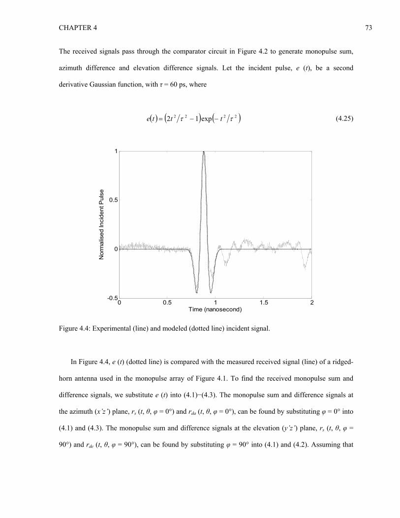
CHAPTER 4 73

The received signals pass through the comparator circuit in Figure 4.2 to generate monopulse sum,

azimuth difference and elevation difference signals. Let the incident pulse, e (t), be a second

derivative Gaussian function, with τ = 60 ps, where

( ) ( ) ( )2222 exp12 ττ ttte −−= (4.25)

In Figure 4.4, e (t) (dotted line) is compared with the measured received signal (line) of a ridged-

horn antenna used in the monopulse array of Figure 4.1. To find the received monopulse sum and

difference signals, we substitute e (t) into (4.1)−(4.3). The monopulse sum and difference signals at

the azimuth (x’z’) plane, rs (t, θ, φ = 0°) and rda (t, θ, φ = 0°), can be found by substituting φ = 0° into

(4.1) and (4.3). The monopulse sum and difference signals at the elevation (y’z’) plane, rs (t, θ, φ =

90°) and rde (t, θ, φ = 90°), can be found by substituting φ = 90° into (4.1) and (4.2). Assuming that

0 0.5 1 1.5 2-0.5

0

0.5

1

Time (nanosecond)

Nor

mal

ised

Inci

dent

Pul

se

Figure 4.4: Experimental (line) and modeled (dotted line) incident signal.

CHAPTER 4 74

the impulse responses of the sum and difference monopulse array is defined in (4.22)−(4.24), rs (t, θ,

φ = 0°), rda (t, θ, φ = 0°), rs (t, θ, φ = 90°) and rde (t, θ, φ = 90°) can be derived as

( ) ( ) ( ) ( ) ( )2 2

1 1 1 1, , 0 ' ' ' '2 sins

cr t m t m t m t m tα β β ατθ φ τ τ τ τ

θ⎡ ⎤= ° = + − + + − − −⎣ ⎦

(4.26)

( ) ( ) ( ) ( ) ( )2 2

, , , ,, , 0 ' ' ' '2 sinda i i i i


θ⎡ ⎤= ° = + − + − − + −⎣ ⎦

(4.27)

( ) ( ) ( ) ( ) ( )2 2

2 2 2 2, , 90 ' ' ' '2 sins


θ⎡ ⎤= ° = + − + + − − −⎣ ⎦

(4.28)

( ) ( ) ( ) ( ) ( )2 2

, , , ,, , 90 ' ' ' '2 sinde i i i i


θ⎡ ⎤= ° = + − + − − + −⎣ ⎦

(4.29)

where m’ (t) is the first derivative Gaussian signal expressed as

( ) ( )2 2 2' 2 expm t t tτ τ= − − (4.30)

τα1, τα2, τβ1 and τβ2 of (4.26)−(4.29) are delays expressed as τα1 = (s1 + d1) sin θ / 2c, τα2 = (s2 + d2)

sin θ / 2c, τβ1 = (s1 − d1) sin θ / 2c, and τβ2 = (s2 − d2) sin θ. It is noted here that (4.26) and (4.28) are

even functions of θ, while (4.27) and (4.29) are odd functions of θ. This even / odd property of the

sum / difference signal enables the monopulse receiver to decide on whether the incident signal is

located at the left or right half plane.

The theoretical reference signals for cross-correlation, rs0 (t), rda0 (t) and rde0 (t), can be found by

substituting appropriate angle values into (4.26)−(4.29). Since the sum signal has maximum

amplitude at boresight, the theoretical sum channel reference signal, rs0 (t), can be found by

substituting θ = φ = 0° into (4.26),

( ) ( )0 , 0 , 0s sr t r t θ φ= = ° = ° (4.31)

CHAPTER 4 75

The angle where rda (t) of (4.27) is at global maximum is θA and the angle where rde (t) of (4.29) is

at global maximum be θE. Because rda (t) and rde (t) are odd functions of θ, the angles at which they

are at global minimum are −θA and −θE. Numerical method is used to find these angles. Once found,

θA and θE, are then substituted back into (4.27) and (4.29),

( ) ( )0 , , 0da da Ar t r t θ θ φ= = = ° (4.32)

( ) ( )0 , , 90de de Er t r t θ θ φ= = = ° (4.33)

The ideal sum channel reference signal (4.31) can be generated since it is a second derivative

Gaussian function. The ideal difference channel reference signals, (4.32) and (4.33), however, are

complex and difficult to generate. To simplify the pulse generation process, we approximate (4.32)

and (4.33) with first derivative Gaussian pulses, aDA (t) and aDE (t), where

( ) ( ) ( )2 2 22 expDA DA DAa t t d t d= − − (4.34)

( ) ( ) ( )2 2 22 expDE DE DEa t t d t d= − − (4.35)

with pulse widths of dDA and dDE. dDA can be calculated from the time difference between the instance

when rda0 (t) (4.27) is maximum, tmax (rda0), and the instance when rda0 (t) (4.27) is minimum, tmin (rda0);

while dDE can be calculated from the time difference between the instance when rde0 (t) (4.29) is

maximum, tmax (rde0), and the instance when rde0 (t) (4.29) is minimum, tmin (rde0),

( ) ( )max 0 min 012DA rda rdad t t= − (4.36)

( ) ( )max 0 min 012DE rde rded t t= − (4.37)

CHAPTER 4 76

To illustrate the calculation of the sum and difference reference signals, let the incident signal be

second derivative Gaussian pulse as shown in (4.25), and the aperture field distribution functions of

the receiving array be (4.19)−(4.21). θA can be found as 3.9°. Figure 4.5 compares the measured

difference signal at azimuth plane (θ = θA = 3.9°) with theoretical difference signal (4.32) and

approximated reference signal (4.34). By coding (4.27) in MATLAB code to find the global

maximum and global minimum points for all values of t and θ, the time difference between the

instances of global maximum and global minimum in (4.27) is found to be 73 ps. By substituting the

time difference into (4.36), it can be shown that dDA = 52 ps. Furthermore, by substituting dDA into

(4.34), the approximated reference signal aDA (t) can be plotted out, as shown in Figure 4.5.

Using (4.34) and (4.35) as reference signals for the cross-correlation receivers in Figure 4.4 are

valid only if the incident UWB signal has a pulse shape of (4.25). UWB monopulse radars employing

0 0.5 1 1.5 2-3

-2.5

-2

-1.5

-1

-0.5

0

0.5

1

Time (nanosecond)

Diff

eren

ce C

hann

el R

efer

ence

Sig

nals

measured difference signal at θ = 4°

theoretical difference signal at θ = 3.9°

approximate difference channel reference signal, aDA(t)

0 0.5 1 1.5 2-3

-2.5

-2

-1.5

-1

-0.5

0

0.5

1

Time (nanosecond)

Diff

eren

ce C

hann

el R

efer

ence

Sig

nals

measured difference signal at θ = 4°

theoretical difference signal at θ = 3.9°

approximate difference channel reference signal, aDA(t)

Figure 4.5: Theoretical, measured and approximate difference signal in the azimuth plane for θ = θA ≈

3.9°.

CHAPTER 4 77

other pulse shapes can derive their respective reference signals based on the method proposed in this

section. However, should the incident signal suffers slight pulse distortion from (4.25), the monopulse

receiver still remains functional, although with degraded performance. The rate of performance

degradation is proportional to the extent of pulse distortion. By cross-correlating the sum channel

reference signal (4.31) with the received sum signal (4.26) and (4.28), we can derive the azimuth sum

output voltage, S (θ, 0), and the elevation sum output voltage, S (θ, π / 2). By cross-correlating the

azimuth / elevation difference channel reference signal (4.34) and (4.35) with the received azimuth /

elevation difference signal (4.27) and (4.29), we can derive the azimuth difference output voltage, DA

(θ, 0), and the elevation difference output voltage, DE (θ, π / 2). The derived output voltages are

expressed as follow:

( )( ) ( )( ) ( )

4 1 1

1 1

''' , ''' ,, 0 max

4 sin ''' , ''' ,

s s s s

s s s s

m t d m t dS

m t d m t d

α β

β α

τ τ τ τ τ ττθθ τ τ τ τ τ τ

⎧ ⎫⎡ ⎤+ − + − + − +⎪ ⎪⎢ ⎥= ⎨ ⎬⎢ ⎥+ − − + − − − +⎪ ⎪⎣ ⎦⎩ ⎭

(4.38)

( ) ( )( ) ( )

4 2 2

2 2

''' , ''' ,, max

2 4 sin ''' , ''' ,

s s s s

s s s s

m t d m t dS

m t d m t d

α β

β α

τ τ τ τ τ τπ τθθ τ τ τ τ τ τ

⎧ ⎫⎡ ⎤+ − + − + − +⎪ ⎪⎛ ⎞ ⎢ ⎥= ⎨ ⎬⎜ ⎟ ⎢ ⎥⎝ ⎠ + − − + − − − +⎪ ⎪⎣ ⎦⎩ ⎭

(4.39)

( )( ) ( )( ) ( )

41 1

1 1

'' , '' ,, 0 max

4 sin '' , '' ,DA DA DA DA

ADA DA DA DA

m t d m t dD

m t d m t dα α

α α

τ τ τ τ τ ττθθ τ τ τ τ τ τ

⎧ ⎫⎡ ⎤+ − + − + − +⎪ ⎪= ⎢ ⎥⎨ ⎬− − − + + + − +⎢ ⎥⎪ ⎪⎣ ⎦⎩ ⎭

(4.40)

( ) ( )( ) ( )

42 2

2 2

'' , '' ,, max

2 4 sin '' , '' ,DA DA DA DA

EDA DA DA DA

m t d m t dD

m t d m t dα α

α α

τ τ τ τ τ τπ τθθ τ τ τ τ τ τ

⎧ ⎫⎡ ⎤+ − + − + − +⎪ ⎪⎛ ⎞ = ⎢ ⎥⎨ ⎬⎜ ⎟ − − − + + + − +⎝ ⎠ ⎢ ⎥⎪ ⎪⎣ ⎦⎩ ⎭

(4.41)

where m’’(t, τ) and m’’’(t, τ) are the second and third derivatives of Gaussian function, expressed as

( ) ( ) ( )2 2 2 2 2'' , 2 2 1 expm t t tτ τ τ τ= − − (4.42)

( ) ( ) ( )4 2 2 2 2''' , 4 3 2 expm t t t tτ τ τ τ= − − (4.43)

CHAPTER 4 78

4.4 Measurements

Measurements are conducted to validate the sum and difference waveforms given in

(4.26)−(4.29), the azimuth sum channel pattern (4.38), and the azimuth difference channel pattern

(4.40). Figure 4.6 shows the experimental setup to measure time-domain received monopulse sum

and difference signals at various angles. A pulse source with Vp-p = 2.0 V, PRF = 1 MHz and Jitter =

1.5 ps (rms) is used as transmitter. The receiver consists of two identical ridged-horn antennas placed

side-by-side as a one-dimension monopulse receiver. This arrangement restricts the monopulse

measurement to azimuth plane only. The return loss of the ridged-horn antenna is less than -10 dB

over 1 to 18 GHz. The ridged-horns are connected to a 180° hybrid-coupler with 3-dB bandwidth

from 1 to 12.4 GHz. In the measurements, the hybrid-coupler introduces some signal distortion.

Furthermore, the amplitude and phase mismatches in the hybrid-coupler may result in inefficient

combining of the antenna outputs to form the monopulse sum and difference signals. These

imperfections, however, are negligible, and not modeled in the derivations. The sum and difference

signals of the coupler are recorded by a 40 GS/s sampling oscilloscope, averaged at 1,024 times.

10.0 m

3.0

m

12.4 m

> 20 m

> 20 mground

6.2 mturn-table

transmittermonopulse

receiver

10.0 m

3.0

m

12.4 m

> 20 m

> 20 mground

6.2 mturn-table

transmittermonopulse

receiver

Figure 4.6: Experimental setup to measure the received monopulse sum and difference signals.

CHAPTER 4 79

The receiving monopulse array is placed on a turn-table so that the axis of the rotation is located

in the middle of the apertures. The sum and difference signals are measured from -20° to 20° in steps

of 1°. To find the sum and difference patterns at the output of the cross-correlation receiver, the

measured signals are mathematically correlated with reference signals (4.31), (4.34) and (4.35)

derived in Section 4.3. The presence of ridges in a horn concentrates the field intensity at the middle

of the horn aperture. Hence, a rectangular aperture function used in Section 4.3 may not be an

accurate approximation for the aperture field distribution. To obtain a better approximation of the

aperture field distribution, we model it as a 12-th power half-cosine function. Figure 4.7 plots the

normalized energy pattern, as defined in Chapter 2, of antenna aperture functions of rectangular shape

(Trace 1), cos2 shape (Trace 2), cos4 shape (Trace 3), cos8 shape (Trace 4) and cos12 shape (Trace 5).

It is observed in Figure 4.7 that when n = 12, the aperture function provides the best fit with the

measured radiation pattern (Trace 6).

-40 -20 0 20 400

0.2

0.4

0.6

0.8

1

Incident Angle (Degrees)

Nor

mal

ized

Ene

rgy

Pat

tern

Trace 1Trace 2Trace 3Trace 4Trace 5

Trace 7

Trace 6

-40 -20 0 20 400

0.2

0.4

0.6

0.8

1

Incident Angle (Degrees)

Nor

mal

ized

Ene

rgy

Pat

tern

Trace 1Trace 2Trace 3Trace 4Trace 5

Trace 7

Trace 6

Legend: - Trace 1 shows radiation pattern when aperture field is approximated by rectangular function. - Traces 2-6 show the radiation patterns when the approximations are cos1, cos2, cos4, cos8 and cos12

functions. - Trace 7 shows the measured radiation pattern of a single ridged-horn. Figure 4.7: Comparison between measured normalized energy pattern of a single ridged-horn with the

normalized energy patterns derived from various theoretical aperture functions.

CHAPTER 4 80

Hence, the impulse response of the sum and azimuth difference monopulse array can be re-

written as,

( )( )( )

( ) ( )( )

( )1 1 1 11 112 12

1 1 1 1

, , 0 cos cossin sin sin

s d s ds ss

s d s d

u t u tc t c tcf td du t u t

τ τ τ τπ τ π τθ φ

θ θ θτ τ τ τ

⎧ ⎫⎡ ⎤ ⎡ ⎤− − − + − −⎡ ⎤ ⎡ ⎤− +⎪ ⎪= ° = +⎢ ⎥ ⎢ ⎥⎨ ⎬⎢ ⎥ ⎢ ⎥− + + +⎢ ⎥ ⎢ ⎥⎣ ⎦ ⎣ ⎦⎪ ⎪⎣ ⎦ ⎣ ⎦⎩ ⎭

(4.44)

( )( )( )

( ) ( )( )

( )1 1 1 11 112 12

1 1 1 1

, , 0 cos cossin sin sin

s d s ds sad

s d s d

u t u tc t c tcf td du t u t

τ τ τ τπ τ π τθ φ

θ θ θτ τ τ τ

⎧ ⎫⎡ ⎤ ⎡ ⎤− − − + − −⎡ ⎤ ⎡ ⎤− +⎪ ⎪= ° = −⎢ ⎥ ⎢ ⎥⎨ ⎬⎢ ⎥ ⎢ ⎥− + + +⎢ ⎥ ⎢ ⎥⎣ ⎦ ⎣ ⎦⎪ ⎪⎣ ⎦ ⎣ ⎦⎩ ⎭

(4.45)

Numerical results of sum and difference signals for a monopulse receiver consisting of ridge-

horns with cos12 aperture function are compared with the measured signals in Figures 4.8 and 4.9. The

sum and difference signals, as shown in Figures 4.8 and 4.9, are cross-correlated with the reference

signals (4.31), (4.34) and (4.35) to generate the monopulse output signals. As seen from the

monopulse receiver in Figure 4.3, the monopulse output signals are constant voltage values that

correspond to a particular target angle. The angle-dependent monopulse values for θ from −20° to 20°

are shown in Figure 4.10 (line), for sum channel, and Figure 4.11 (line), for difference channel. Both

Figures 4.10 and 4.11 show that the theoretical monopulse output voltages based on the rectangular

aperture function (dotted line) and the cos12 aperture function (dashed line).

CHAPTER 4 81

0 0.5 1 1.5 2-2.5

-2

-1.5

-1

-0.5

0

0.5

1

1.5

2

2.5

Time (ns)

Nor

mal

ised

Am

plitu

de

θ = -20°

θ = -10°

θ = 0°

θ = 10°

θ = 20°

0 0.5 1 1.5 2-2.5

-2

-1.5

-1

-0.5

0

0.5

1

1.5

2

2.5

Time (ns)

Nor

mal

ised

Am

plitu

de

θ = -20°

θ = -10°

θ = 0°

θ = 10°

θ = 20°

Figure 4.9: Comparison between simulated (dotted line) and measured (line) difference signals for θ =

−20°, −10°, 0°, 10° and 20°.

0 0.5 1 1.5 2-2.5

-2

-1.5

-1

-0.5

0

0.5

1

1.5

2

2.5

Time (ns)

Nor

mal

ised

Am

plitu

de

θ = -20°

θ = -10°

θ = 0°

θ = 10°

θ = 20°

0 0.5 1 1.5 2-2.5

-2

-1.5

-1

-0.5

0

0.5

1

1.5

2

2.5

Time (ns)

Nor

mal

ised

Am

plitu

de

θ = -20°

θ = -10°

θ = 0°

θ = 10°

θ = 20°

Figure 4.8: Comparison between simulated (dotted line) and measured (line) sum signals for θ =

−20°, −10°, 0°, 10° and 20°.

CHAPTER 4 82

Nor

mal

ized

Diff

eren

ce C

hann

el C

ross

-cor

rela

tion

Out

puts

-20 -15 -10 -5 0 5 10 15 20-1

-0.8

-0.6

-0.4

-0.2

0

0.2

0.4

0.6

0.8

1

Degree (Theta)

Measured

cos12 aperture function

rectangular aperture function

Nor

mal

ized

Diff

eren

ce C

hann

el C

ross

-cor

rela

tion

Out

puts

-20 -15 -10 -5 0 5 10 15 20-1

-0.8

-0.6

-0.4

-0.2

0

0.2

0.4

0.6

0.8

1

Degree (Theta)

Measured


rectangular aperture function

Figure 4.11: Theoretical and measured monopulse difference channel cross-correlation output. The

theoretical monopulse sum outputs are calculated based on rectangular aperture function (dotted line) and cos12 aperture function (dashed line).

-20 -15 -10 -5 0 5 10 15 200

0.1

0.2

0.3

0.4

0.5

0.6

0.7

0.8

0.9

1

Theta (Degrees)

Measured


rectangularaperture function

Nor

mal

ized

Sum

Cha

nnel

Cro

ss-c

orre

latio

n O

utpu

t

-20 -15 -10 -5 0 5 10 15 200

0.1

0.2

0.3

0.4

0.5

0.6

0.7

0.8

0.9

1

Theta (Degrees)

Measured


rectangularaperture function

Nor

mal

ized

Sum

Cha

nnel

Cro

ss-c

orre

latio

n O

utpu

t

Figure 4.10: Theoretical and measured (line) monopulse sum channel cross-correlation output. The

theoretical monopulse sum outputs are calculated based on rectangular aperture function (dotted line) and cos12 aperture function (dashed line).

CHAPTER 4 83

The signal used by the amplitude-comparison monopulse processor to determine the angle-of-

arrival of the incident signal is the monopulse ratio, which is the ratio of D (θ) over S (θ). This ratio

ensures that the monopulse processor output depends only on the incident angle, and not on the target

range and radar cross-section [58]. Based on the cross-correlation outputs of the sum and azimuth

difference channels that are derived with cos12 aperture function, the theoretical monopulse ratio is

plotted (line) in Figure 4.12 and compared with measured (circles) incident signals at 1° intervals

from −20° to +20°. As can be seen from Figure 4.12, the unambiguous tracking range of this

monopulse radar is ± 6°. The radar’s angular resolution, defined as its ability to resolve many targets

[23], is dependent on array beamwidth, which is 6° in this configuration. The proposed model

accurately predicts the performance of the UWB monopulse radar in terms of signal shapes, receiver

patterns and the monopulse ratio.

-20 -15 -10 -5 0 5 10 15 20-1

-0.8

-0.6

-0.4

-0.2

0

0.2

0.4

0.6

0.8

1

Mon

opul

se R

atio

TheoreticalMeasured

Incident angle (Degrees)-20 -15 -10 -5 0 5 10 15 20-1

-0.8

-0.6

-0.4

-0.2

0

0.2

0.4

0.6

0.8

1

Mon

opul

se R

atio

TheoreticalMeasured

Incident angle (Degrees) Figure 4.12: Comparison between theoretical (line) and measured (circles) monopulse ratio. The

theoretical (line) monopulse ratio is derived based on ridged-horn aperture functions that are defined by cos12 functions.

CHAPTER 4 84

The effects of antenna configuration and received signal shape on the Monopulse ratio are studied.

In the first study, the aperture size of the individual horns is increased, and the effect of this variation

to the Monopulse ratio is plotted out in Fig. 4.13. The net effect of increasing the aperture size of the

individual horns of the Monopulse square-feed array is that the directivity of both the sum and

difference modes of the array has increased, because the directivity of its constituent horns has

increased. As shown in Fig. 4.14, the angular range and accuracy of the Monopulse tracking is

changed when this happens – with increased directivity of the individual horns, the angular range of

the Monopulse tracking is reduced, while the accuracy of the tracking is increased. This variation of

Monopulse tracking performance can be utilized by the transceiver designer to design either a highly

accurate tracking Monopulse receiver, or a large angular range tracking Monopulse receiver with a

decreased tracking accuracy.

-20 -15 -10 -5 0 5 10 15 20-1

-0.5

0

0.5

1

Incident angle (degrees)

Mon

opul

se R

atio

dotted line:dashed line:

line:circles:

crosses:

d = 35 cmd = 30 cmd = 25 cmd = 20 cmd = 15 cm

-20 -15 -10 -5 0 5 10 15 20-1

-0.5

0

0.5

1

Incident angle (degrees)

Mon

opul

se R

atio


line:circles:

crosses:



line:circles:

crosses:


Figure 4.13: The effect of the antenna aperture length on the Monopulse ratio and the performance of

the Monopulse tracking receiver.

CHAPTER 4 85

In the second study, the pulse-width of the incident signal is varied, and its effect on the Monopulse

ratio is observed in Fig. 4.14. The net effect of reducing the pulse-width of the incident signal is to

increase the frequency component of the incident signal. As can be observed from Fig. 4.14, reducing

the pulse-width of the incident signal increases the angle accuracy of the Monopulse receiver while it

also narrows the angular range of the Monopulse ratio.

4.5 Antenna Noise Effect on Receiver

Let the output of the monopulse comparator circuit in Figure 4.3 be corrupted by additive thermal

noise due to the antenna noise of the antennas of the monopulse array [10]. Let the noise corrupted

sum and azimuth difference signals be modeled as rsn (t) and rdan (t), where

( ) ( ) ( ) ( )0 ,sn sr t e t f t n tτ σ= − ⊗ + (4.46)

-20 -15 -10 -5 0 5 10 15 20-1

-0.5

0

0.5

1

Incident Angle (degrees)

Mon

opul

se R

atio


line:circles:

crosses:

τ = 40 psτ = 50 psτ = 60 psτ = 70 psτ = 80 ps

-20 -15 -10 -5 0 5 10 15 20-1

-0.5

0

0.5

1

Incident Angle (degrees)

Mon

opul

se R

atio


line:circles:

crosses:



line:circles:

crosses:


Figure 4.14: The effect of the incident signal’s pulse-width on the Monopulse ratio and the

performance of the Monopulse tracking receiver.

CHAPTER 4 86

( ) ( ) ( ) ( )0 ,dan adr t e t f t n tτ σ= − ⊗ + (4.47)

τ0 is the true time-of-arrival of the incident signal, e (t). fs (t) and fad (t) are the impulse responses

of the monopulse array in sum and azimuth channels defined in (4.44) and (4.45) respectively. n (t) is

the antenna noise, modeled as Additive White Gaussian Noise of energy σ2. Similar to the noise

analysis in Chapter 3, σ2 is related to N0 and antenna temperature, Tant as σ2 = N0 = kTant, where k is

the Boltzmann’s constant. The time-of-arrival of the signals is estimated from the sum channel

waveform, rsn (t). Similar to the derivations in (3.7)−(3.18), assuming that the ratio of sum channel

signal energy to noise energy is much greater than 1, i.e. Es (θ) / N0 >> 1, the estimated time-of-

arrival of rsn (t) can be approximated to be

0τ ~ ( ) ( ) 20 0, s sN N Eτ θ β θ⎡ ⎤⎣ ⎦ (4.48)

Es (θ) and βs2 (θ) can be expressed as

( ) ( ) ( ) ( )00

,T

s s sE e t f t r t dtθ θ⎡ ⎤= ⊗⎣ ⎦∫ (4.49)

( ) ( ) ( ) ( ) ( )2

202

0

,T

s ad sdE e t f t r t dtdt

β θ θ θ⎡ ⎤= ⊗⎣ ⎦∫ (4.50)

Measurements of received monopulse sum signal, for θ = −5° to 5° in 1° intervals, have been

conducted to verify the standard deviation of theoretical time-of-arrival, as predicted in (4.48). For

each angle, 50 sets of received monopulse sum signal have been measured in accordance to the

measurement setup described in Section 3.5. The measurement of received signals is performed for

one SNR levels. The measured sum signals have been cross-correlated with the sum channel

reference signal, rs0 (t), to find the estimated time-of-arrival, 0τ . The thermal noise signal that is

CHAPTER 4 87

corrupting the monopulse sum signal has also been measured, and the mean noise power per

bandwidth is found to be N0 = 6.2e-19 J.

To find the energy of the noiseless received signal at boresight, Es (θ = 0°), the sum signal is

averaged 4096 times to suppress the noise contribution. The measured Es (θ = 0°) is 4.4e-16 J for a

received signal amplitude of 2.8 mV. Hence, the signal-to-noise ratios (SNR) at which the monopulse

receiver is experimented upon is +28.5 dB. Figure 4.13 shows the comparison between theoretical

(line) and measured (circle) standard deviations of estimated time-of-arrivals for the case where the

SNR is +28.5 dB. From Figure 4.15, it can be observed that the measured standard deviations of TOA

for all measured angles are close to the theoretical standard deviations.

The monopulse radar finds the angle-of-arrival of the incident signal by finding the monopulse

ratio, as shown in Figure 4.12. The process of estimating the monopulse ratio, however, involves

finding the time-of-arrival of the sum signal first. As shown above, the time-of-arrival of the sum

-5 -4 -3 -2 -1 0 1 2 3 4 50

1

2

3

4

5

6

7

8

Incident angle (Degrees)

Stan

dard

Dev

iatio

n of

TO

A (p

s)

-5 -4 -3 -2 -1 0 1 2 3 4 50

1

2

3

4

5

6

7

8

Incident angle (Degrees)

Stan

dard

Dev

iatio

n of

TO

A (p

s)

Figure 4.15: Comparison between theoretical (line) and measured (circles) standard deviations of

time-of-arrival (TOA) for different angles.

CHAPTER 4 88

signal follows the probability density function of (4.40). Hence, the probability density function of the

monopulse ratio, R , can be expressed as

( ) ( )( ) ( )

0 0

0 0

ˆ ˆ ˆ,ˆˆ ˆ ˆ,

d d

s s

v wDRv wS

τ θ ττ θ τ

+= =

+ (4.51)

where

( ) ( ) ( ) ( )0 0 0 00ˆ ˆ,

T

s s sv r t f t r t dtτ θ τ τ⎡ ⎤= − ⊗ −⎣ ⎦∫ (4.52)

( ) ( ) ( )0 0 00ˆ ˆ, ,

T

s sw n t r t dtτ σ σ τ= −∫ (4.53)

( ) ( ) ( ) ( )0 0 00ˆ ˆ,

T

d ad dav r t f t r t dtτ θ τ τ⎡ ⎤= − ⊗ −⎣ ⎦∫ (4.54)

( ) ( ) ( )0 0 00ˆ ˆ, ,

T

d daw n t r t dtτ σ σ τ= −∫ (4.55)

Applying similar method of derivation as Section 3.3, functions vs and vd are expanded about τ0

with Taylor expansion and only the first three terms are retained,

( ) ( ) ( )2 20 0ˆ ˆ, 1 2s s sv Eτ θ θ β θ τ⎡ ⎤⋅ −⎣ ⎦ (4.56)

( ) ( ) ( )2 20 0ˆ ˆ, 1 2d d dv Eτ θ θ β θ τ⎡ ⎤⋅ −⎣ ⎦ (4.57)

where 0τ is the probability density function of the estimated time-of-arrival, defined in (4.48). Es (θ)

and βs2 (θ) are defined in (4.49) and (4.50), and Ed (θ) and βd

2 (θ) are

CHAPTER 4 89

( ) ( ) ( ) ( )0,d ad daTE e t f t r t dtθ θ⎡ ⎤= ⊗⎣ ⎦∫ (4.58)

( ) ( ) ( ) ( ) ( )2

202,d d ad daT

dE e t f t r t dtdt

β θ θ θ⎡ ⎤= ⊗⎣ ⎦∫ (4.59)

Functions ws (4.53) and wd (4.55) are weighted average n (t), and therefore has a Gaussian

distribution of zero mean [10]. The variance of ws (τ) and wd (τ) can be found by sampling analysis.

Taking an arbitrarily small value of Δt as the lower sampling time limit, ws (τ) and wd (τ) can be

rewritten as

01

T t

s i s ii

w t n rΔ

=

= Δ ∑ (4.60)

01

T t

d i da ii

w t n rΔ

=

= Δ ∑ (4.61)

where rs0i and rda0i are samples of rs0 (t – τ) and rda0 (t – τ) respectively. Each sample of ni has a

variance of N0 / Δt. Since all ni samples are statistically independent, the total variance is the sum of

the variances of each sample,

( )22 200 0

1

T t

s s i rsi

Nw t r N Et

Δ

=

= Δ =Δ∑ (4.62)

( )22 200 0

1

T t

d da i rdi

Nw t r N Et

Δ

=

= Δ =Δ∑ (4.63)

where Ers and Erd are the energy of the reference signals for the sum and difference channel. Hence,

ws and wd are derived as

CHAPTER 4 90

( )00,s rsw N N E∼ (4.64)

( )00,d rdw N N E∼ (4.65)

Comparing the variances between the random variables in the numerator of (4.51), we find that if

Es(θ) >> N0, variance of wd is much greater than variance of vd. Comparing the variances between the

random variables in the denominator of (4.51), we can find that under same condition of Es(θ) >> N0,

variance of ws is much greater than variance of vs. Thus, error contributions by vs and vd can be

neglected. Hence, R can be rewritten as

( )( )

ˆ d d

s s

E wR

E wθθ

+=

+ (4.66)

The probability density function of estimated angle-of-arrival, θ , can be obtained by dividing the

estimated monopulse ratio, R , with the true monopulse ratio in Figure 4.12, and then multiplying

with the true angle-of-arrival,

( )( )

( )( )

1ˆ ˆ1

s d d

d s s

E w ER

E w Eθ θ

θ θ θθ θ

+= =

+ (4.67)

Equation (4.67) is a ratio of two independent random variables, which is difficult to resolve.

Further simplification can be done by approximating the denominator of (4.67) to one, since

( ) ( ) ( )20var 0 1s sw E N E Eθ θ θ⎡ ⎤ = =⎣ ⎦ (4.68)

CHAPTER 4 91

The error contribution of the random variable at the denominator is neglected. Hence, the

estimated angle-of-arrival is approximately

( )ˆ 1 d dw Eθ θ θ⎡ ⎤+⎣ ⎦ (4.69)

Thus, the standard deviation (root-mean-square error) of angle estimate for the proposed

monopulse radar is derived from (4.69) as

( )ˆ 0 rd dN E Eθ

σ θ θ (4.70)

In Figure 4.16, the standard deviations of estimated angle-of-arrival, as derived in (4.70), are

calculated and then compared with angle-of-arrival measurements for the angles −5° to +5°. In the

measurement, the same receiver setup in Section 4.4 is used. A UWB signal source is placed in far-

field distance, transmitting signal in a power levels similar to the case above where the SNR is +28.5

dB. 50 sets of sum and difference signals are measured for each angle, where the monopulse ratio and

the angle-of-arrival are estimated from each of the measured signals. The standard deviation of the

angle-of-arrival accuracy is then calculated from the values of the 50 measured samples. Figure 4.16

shows the theoretical and measured standard deviation of angle-of-arrival accuracy of the monopulse

receiver for the case when SNR = +28.5 dB. The theoretical standard deviations are less than

measurements because of the approximations applied underestimate the errors. Figure 4.16 shows a

significant rise in error at angles near boresight because the receiver is unable to decide whether the

monopulse processor output is from left-hand-side of the antenna, or the right-hand-side.

CHAPTER 4 92

4.6 Chapter Summary

In this chapter, we have proposed an amplitude-comparison monopulse receiver for ultra-

wideband (UWB) receivers. The receiver captures the incident signal with a square-feed array of four

ridged-horns. Based on the aperture field distribution functions of the ridged-horns, we have derived

the monopulse sum and difference signals. The proposed model has been evaluated with

measurements, and found good agreement between measurement and theory. The angular accuracy of

the monopulse receiver is also derived and verified by measurements.

-5 -4 -3 -2 -1 0 1 2 3 4 50.05

0.1

0.15

0.2

0.25

0.3

0.35

0.4

0.45

0.5

Stan

dard

dev

iatio

n (d

egre

es)

Incident angle (Degrees)-5 -4 -3 -2 -1 0 1 2 3 4 5

0.05

0.1

0.15

0.2

0.25

0.3

0.35

0.4

0.45

0.5

Stan

dard

dev

iatio

n (d

egre

es)

Incident angle (Degrees) Figure 4.16: Theoretical (line) and measured (circles) standard deviations of angle error for Eb / N0 of

28.5 dB.

CHAPTER 5 93

CHAPTER 5

SUB-NANOSECOND PULSE FORMING NETWORK FOR

UWB TRANSCEIVER

5.1 Introduction

In ultra-wideband (UWB) radio systems, the transmitter needs to generate sub-nanosecond pulses

to be transmitted through the wireless channel. In a UWB radar system, the pulses are transmitted

directly after the pulse generation circuit, and the scattered signal is collected by the receiver. In a

UWB communication system, the generated pulses are further modulated and then transmitted

through the wireless channel. The circuit that generates these pulses is generally called the pulse

forming network (PFN). In this chapter, we propose a novel PFN design to generate electrical pulses

in the sub-nanosecond regime, specifically for the short range UWB radar and the high data rate

UWB communication systems. The proposed PFN is designed to generate pulses at pulse repetition

frequency (PRF) of about 500 MHz at power levels comparable to FCC emission limit [2].

Furthermore, the proposed PFN only consumes a DC power supply of 3.3 V, 20 mA during operation.

The PFN is designed in SiGe BiCMOS for the ease of circuit integration. The PFN circuit occupies a

small area 0.25 mm2, making it suitable to be incorporated into short range (< 0.3 m) UWB radars and

high data rate UWB communication systems like the wireless video streaming and wireless personal

area network (WPAN).

CHAPTER 5 94

As shown in Figure 5.1, the pulse forming network (PFN) can be used in a UWB transceiver in

two ways – to generate pulses in transmitter, and to generate reference signals for the cross-

correlation receivers, as described in the receivers in Chapters 3–5. It is important that the PFN

consumes low DC power supply, especially for portable devices, and generates pulses in sufficiently

high amplitudes without the assistance of additional broadband amplifiers, so that electrical power is

conserved. To meet the FCC’s emission mask [2], the transmitter requires further pulse shaping on

the pulse generated by the PFN. Pulse shaping can be achieved by cascading numerous PFNs to

achieve higher order Gaussian-like pulses [61], cascading the PFN with bandpass filter, or using the

bandpass characteristics of the transmitter antenna. A patent has been filed for this method of

generating UWB pulses [61].

In the open literature, there are many PFNs that are designed for long range UWB radars [30]

−[35]. However, these PFNs are unsuitable for high data rate UWB radio systems because of different

pulse repetition frequency (PRF) requirements of the latter systems. In long range UWB radars,

pulses are generated at medium to high power levels, i.e. watts to kilowatts, and at relatively low PRF,

i.e. few kHz to tens of MHz [41]. In UWB radios [6], [42], and some high pulse rate UWB radar

systems, however, pulses are generated at lower power levels and at higher PRF. UWB radios may

require PRF to be in the order of several hundred MHz to GHz, for high data rate transmission in

Data PulseFormingNetwork

(optional)Pulse

Shaper

UWB Transmitter

ControlPulse

FormingNetwork

correlator Data

UWB Receiver

Data PulseFormingNetwork

(optional)Pulse

Shaper

UWB Transmitter

ControlPulse

FormingNetwork

correlator Data

UWB Receiver

Figure 5.1: A time domain UWB transceiver using the pulse forming network in the transmitter and

receiver.

CHAPTER 5 95

hundreds of Mbps to Gbps. UWB radars may require PRF to be in the order of several MHz to

several hundred of MHz. Furthermore, a UWB radio system needs to be implemented in silicon

integrated circuit to be economical in volume production. Pulse forming methods for long range

UWB radars require specialized components like Step-Recovery Diodes [39], [40], avalanche

transistors, non-linear transmission lines [37] etc. which are not amenable to implementation in

silicon integrated circuit.

An alternative and popular method for generating pulses for high data rate UWB radio can be

found in [3]. In this method, a differential clock signal is used as source signal. One of the differential

signal pair is fed into more delay buffers than the other, creating two single ended clock signals of

different delays. The two single ended signals are then combined using an exclusive OR gate to form

a sub-nanosecond pulse.

This chapter describes the theory, design, fabrication and measurement of our proposed pulse

forming network (PFN). Section 5.2 presents the theory and schematic design of the PFN circuit.

Section 5.3 presents the layout design, fabrication and measurement methodology of the fabricated

circuit. Finally, Section 5.4 presents the experimental results and compares them with theoretical and

simulated results.

5.2 Schematic Design of the Pulse Forming Network

In this section, we will present the schematic design of the pulse forming network (PFN). It is

necessary to determine the required system specification. 5.2.1 presents two intended applications of

the PFN and the PFN’s system specification. Next, in 5.2.2 and 5.2.3, the PFN is designed based on

the stated system specifications. The PFN is designed based on the strategy of performing time

derivative on an input step signal. In 5.2.2, we will present a circuit that enhances the input step signal

so that the characteristics of the PFN’s output pulses do not deteriorate with input signal deterioration.

CHAPTER 5 96

In 5.2.3, we present the design of a transistor-base differentiation circuit that generates the pulses for

the PFN.

5.2.1 System Requirement of the Pulse Forming Network

In this section, we will find the required system specification of the PFN based on the intended

applications. To do so, we need to first look into the requirements of a transceiver system that

incorporates the proposed PFN to transmits data at 500 MHz PRF. A possible high data rate

application is the UWB video streaming from set-up box to High-Definition Television (HDTV) and

speakers for home entertainment system. The radio system required for this video streaming

application is a UWB transmitter with directional antenna, placed at the set-up box, to transmit video

data to a UWB receiver that is placed at the HDTV.

A possible transmitter design for the above application is shown in Figure 5.2. The transmitter

first codes the data with Manchester coding, and then generates the sub-nanosecond UWB pulses

from the digital coded data signal. The output pulses from the PFN are shaped by a bandpass filter to

meet FCC limit on the transmitter’s EIRP [2] of −41.25 dBm/MHz from 3.1 – 10.5 GHz, and then

transmit the signal with a directional antenna [4]. Directional antenna is used here, instead of omni-

Data

ManchesterCode

PulseFormingNetwork

BandpassFilter

Data

ManchesterCode

PulseFormingNetwork

BandpassFilter

Figure 5.2: Schematic diagram of a time domain UWB transmitter using the pulse forming network.

CHAPTER 5 97

directional antenna, because it is more suitable for the directional wireless data transmission from the

set-up box to the HDTV. Multiple directional antennas have also been used for transmitter diversity

to enhance wireless performance. It is assumed that antenna gain of 7 dBi is used for directional

coverage in video streaming applications. It is also assumed that there is a 3 dB insertion loss between

the connection from the PFN’s output to antenna input. With these assumptions, it can be calculated

that the required output power spectral density of the PFN needs to be −44.25 dBm/MHz from 3.1 to

10.5 GHz.

Another possible application of the PFN is in short range (< 0.3 m) UWB radars. Figure 5.3

shows the transceiver architecture of a short range radar with single transmit/receive antenna. The

pulse forming is used as a signal source to be fed to port 1 of the 180° hybrid coupler through a

bandpass filter that pulse shapes the PFN output. The hybrid coupler acts as duplexer between the

transmitter (port 1) and the receiver (port 2) of the radar. The antenna is connected to the sum port

(port ‘S’), and a directional antenna is used as both transmit and receive antenna. A matched load (Z0

= 50 Ω) is connected at the difference port (port ‘D’) to ensure no signal from the transmitter chain

(port 2) is leaked to the receiver chain (port 3). The received signal from the antenna is coupled to

port 2 of the hybrid coupler with 3-dB loss. The signal is amplified with a low noise amplifier (LNA)

BandpassFilter

180°3-dB

Hybrid Coupler

LNABandpass

Filter

IntegrationCircuit Z0

1

2

S

D

Signal Detection

Pulse FormingNetwork


BandpassFilter

180°3-dB

Hybrid Coupler

LNABandpass

Filter

IntegrationCircuit Z0

1

2

S

D

Signal Detection



Figure 5.3: Schematic diagram of a time domain UWB radar using the pulse forming network.

CHAPTER 5 98

and then cross-correlated with a reference signal, which is generated by another PFN, and pulse

shaped by a different bandpass filter. For the short range radar, we assume that the same directional

antenna (~7 dBi gain) is used, and a 3 dB loss between the output of the PFN to the input of the

antenna. Hence, the requirement for the PFN used in the radar is the same as that of the wireless

HDTV transmitter.

It can be shown, by simulation, that for a Gaussian-shaped pulse with 175 ps pulse width, to

achieve the output power spectral density of −44.25 dBm/MHz, the pulse should have an amplitude

of 0.15 V and a PRF of 500 MHz. The output Gaussian-shaped pulse train, however, contains spectral

components at frequencies below 3.1 GHz which are undesirable for transmission. These spectral

components can be filtered out by pulse shaping the PFN’s output with any of the methods described

in Section 5.1. Hence, the system requirement for the PFN is to generate an output Gaussian-shape

pulse with 175 ps pulse width, 0.15 V amplitude and 500 MHz PRF.

5.2.2 Input Signal Enhancing Circuit

In this section, a circuit to enhance the input signal to the differentiator circuit will be presented.

A major limitation to performing time derivative on an input digital signal is to ensure a consistent

output pulse amplitude and pulse shape. This is because the input signal may have varying rise-times

and fall-times and contain distortions. Distortions in input signal result in undesirable ringing signals

that superimpose on the output pulse train, increasing the noise floor of the transmitted signal.

Furthermore, variation in the input signal’s rise time causes the output pulse to suffer from

degradation of both pulse width and pulse amplitude.

To ensure that the PFN can consistently generate output pulses with sufficiently short rise-times

(~200 ps), we propose that a fast switching circuit, as shown in Figure 5.4, to be inserted before the

differentiation circuit to enhance the input signal. The fast switching circuit consists of a two stage

bipolar junction transistor (BJT) differential pair. The operation of a differential pair is known [60].

CHAPTER 5 99

Using 2-stages of differential pair acting as current-steering switch [71] ensures that the input clock

signal is switched at the highest speed of the transistors, as long as the transistors are not in saturation

during operation. This improves the rise time of the clock signal thus improving the output pulse

shape consistency.

To reduce input offset currents and voltages, precautions are taken in the circuit layout to ensure

that the important components are matched to each other. For example, the resistors R1 are clustered

together in parallel with dummy resistors placed at both sides; Q1 and Q2 transistors are placed in

close proximity, with dummies placed at the sides. The same applies to the current biasing transistors

(Qb1, Qb2 and Qb6).

Transient simulations are done to evaluate the rise-time improvement of the circuit shown in

Figure 5.4. In the simulation, the rise-times of input and output signals are compared, as shown in

Figure 5.5. An 80 ps rise time step signal produces a 30 ps rise time step. If the input rise time is

slowed down by 700 ps, the output rise time only slows down by 53 ps. Figure 5.5 shows that the 2-

A B

A B

C D

VBIAS

VIN+ VIN -

Ib

Qb0 Qb1 Qb2

R1

Q1

R1 R1 R1

Q2 Q1 Q2

VCC

Gnd

A B

A B

C D

VBIAS

VIN+ VIN -

Ib

Qb0Qb0 Qb1Qb1 Qb2Qb2

R1

Q1Q1

R1 R1 R1

Q2Q2 Q1Q1 Q2Q2

VCC

Gnd Figure 5.4: Schematic diagram of the input signal enhancing circuit.

CHAPTER 5 100

stage differential pair is able to reduce the input step rise-time of 800 ps to less than 100 ps, and

reduce rise-time variation to 7.57%. The improvements are the same for positive and negative steps.

5.2.3 Time Derivative Circuit

In this section, we will present the design of time derivative circuit, which will perform time

derivative onto the input step signals to generate pulses at its output. Designing a time derivative

1

1−

⎥⎥⎦

⎤

⎢⎢⎣

⎡+

f

jωω

( )ωX ( )ωYA

( )ωe

_+

( )ωg 1

1−

⎥⎥⎦

⎤

⎢⎢⎣

⎡+

f

jωω

( )ωX ( )ωYA

( )ωe

_+

( )ωg

Figure 5.6: Negative feedback used to realize the differentiator block.

input step rise-time / ns

outp

ut s

tep

rise-

time

/ ps

20

0

40

60

80

100

0.0 0.1 0.2 0.3 0.4 0.5 0.6 0.7 0.8

O – positive stepX – negative step

700 ps

53 p

s

gradient = 0.0757

input step rise-time / ns

outp

ut s

tep

rise-

time

/ ps

20

0

40

60

80

100

0.0 0.1 0.2 0.3 0.4 0.5 0.6 0.7 0.8

O – positive stepX – negative step

700 ps

53 p

s

gradient = 0.0757

Figure 5.5: Plot of output positive step rise-time (o) and output negative slope rise-time (x) for a input

step rise-time.

CHAPTER 5 101

circuit in time domain is equivalent to designing a jω transfer function in frequency domain. One way

to realize this in active circuit is to use a frequency dependent negative feedback system [49], as

shown in Figure 5.6. This transfer function of a frequency dependent negative feedback is

( )( )

11

f

f

jYA

X A jω ωω

ω ω ω+

=+ +

(5.1)

Equation (5.1) can be approximated to become a differentiating function within the frequency

range when 1 < jω / ωf < 1 + A. To realize the system shown in Figure 5.6, the circuit in Figure 5.7

is used. Furthermore, by analyzing the components R2, Q7, Qb5 and Cf in Figure 5.7 in small signal,

the equivalent circuit in Figure 5.8 can be arrived. Correspondingly, rπ, cπ and gm in Figure 5.8 are the

transistor parameters equivalent to the transistors Q7 and Q8 in Figure 5.7; ro in Figure 5.8 is the

equivalent collector-emitter resistance of the transistors Qb5 and Qb6 in Figure 5.7; Cf in Figure 5.8 is

equivalent to the capacitance Cf introduced at the emitter of transistors Q7 and Q8 in Figure 5.7; Zbias

and Zout in Figure 5.8 are the equivalent impedances of the input bias circuit and output impedances

around transistors Q7 and Q8 in Figure 5.7.

R2RL

VBIAS VBIAS

VCC

Gnd

Q7

C D

Cf

Q5

Qb3 Qb5

Q8

Cf

Q6

R2

Qb6 Qb4

transmissionline

R2RL

VBIAS VBIAS

VCC

Gnd

Q7Q7

C D

Cf

Q5Q5

Qb3Qb3 Qb5Qb5

Q8Q8

Cf

Q6Q6

R2

Qb6Qb6 Qb4Qb4

transmissionline

Figure 5.7: The proposed differentiator circuit.

CHAPTER 5 102

The differentiator circuit output is connected to an external, 50 Ω load via an electrically long

transmission line (Figure 5.7 – dashed line; Figure 5.8 – transmission line). The relationship between

output voltage, vo, and input voltage, vi, of Figure 5.8 are shown in (2).

( )( )

0

0

1

1 1 1fo

i m m f m

R j C rvv g r g r j C C gπ π

ω

ω

+= −

+ + + + (5.2)

-20

-15

-10

-5

0Transfer function (dB)

1 2 3 4 5 6 7 8 9 10frequency (GHz)

theoreticalsimulated

-20

-15

-10

-5

0Transfer function (dB)

1 2 3 4 5 6 7 8 9 10frequency (GHz)

theoreticalsimulated

Figure 5.9: Theoretical and simulated frequency response of the differentiator circuit show a linear

gain profile for frequencies 1 – 10 GHz.

cπ gm vbe

vin

Zbias

rπ

Cf ro

Zout

vout

vbe

vf

if

transmissionline

cπ gm vbe

vin

Zbias

rπ

Cf ro

Zout

vout

vbe

vf

if

transmissionline

Figure 5.8: Small signal analysis of the proposed differentiator circuit.

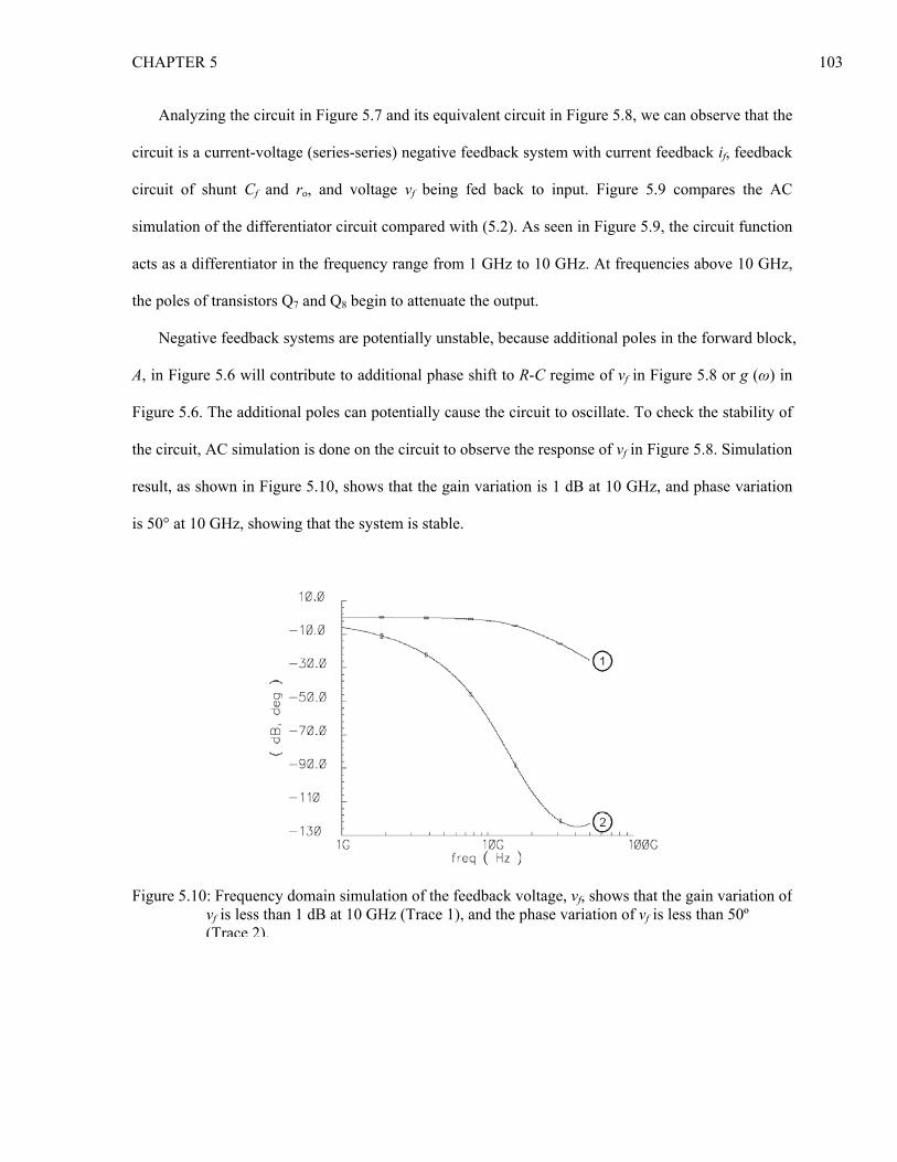
CHAPTER 5 103

Analyzing the circuit in Figure 5.7 and its equivalent circuit in Figure 5.8, we can observe that the

circuit is a current-voltage (series-series) negative feedback system with current feedback if, feedback

circuit of shunt Cf and ro, and voltage vf being fed back to input. Figure 5.9 compares the AC

simulation of the differentiator circuit compared with (5.2). As seen in Figure 5.9, the circuit function

acts as a differentiator in the frequency range from 1 GHz to 10 GHz. At frequencies above 10 GHz,

the poles of transistors Q7 and Q8 begin to attenuate the output.

Negative feedback systems are potentially unstable, because additional poles in the forward block,

A, in Figure 5.6 will contribute to additional phase shift to R-C regime of vf in Figure 5.8 or g (ω) in

Figure 5.6. The additional poles can potentially cause the circuit to oscillate. To check the stability of

the circuit, AC simulation is done on the circuit to observe the response of vf in Figure 5.8. Simulation

result, as shown in Figure 5.10, shows that the gain variation is 1 dB at 10 GHz, and phase variation

is 50° at 10 GHz, showing that the system is stable.

Figure 5.10: Frequency domain simulation of the feedback voltage, vf, shows that the gain variation of

vf is less than 1 dB at 10 GHz (Trace 1), and the phase variation of vf is less than 50º (Trace 2).

CHAPTER 5 104

5.3 Circuit Implementation and Measurements

The pulse forming network (PFN) is fabricated with 0.25 μm SiGe BICMOS process, and

packaged in ASAT Quad Flat Pack. The combined area of the input signal enhancing circuit and time

derivative circuit is 0.25 mm2 (Figure 5.11). This circuit is designed and simulated using Cadence,

and fabricated in IBM SiGe BiCMOS6HP process. Figure 5.11 below show a simple schematic of the

fabricated circuit. In Figure 5.4, an adjustable bias current, Ib, at Qb0 ensures a constant biasing

voltage, Vbias, is applied at Qb1 to Qb6 of Figures 5.4 and 5.7. To ensure performance consistency

amongst Qb1 to Qb6, they are placed close to each other, in a row, with dummy transistors being

placed at both ends. Similar layout method of placing critical components in a row and placing

dummy components at both ends have been applied to the four R1 resistors in Figure 5.4; the two R2

resistors in Figure 5.7; the matched pairs of transistors Q1 and Q2 in Figure 5.4; Q5 and Q6 in Figure

5.7; and Q7 and Q8 in Figure 5.7. Q5 and Q6 are emitter followers that provide isolation between the

signal enhancing circuit and time derivative circuit.

Inpu

t –In

put +

Pulse +

Pulse –

Input SignalEnhancing Circuit

Differentiation Circuit

Inpu

t –In

put +

Pulse +

Pulse –

Input SignalEnhancing Circuit

Differentiation Circuit

Figure 5.11: Magnified picture of the fabricated circuit.

CHAPTER 5 105

Figure 5.11 shows the circuit’s good horizontal symmetry. Two copper lines (extreme left) are the

differential input signal lines. The differential input signal lines are connected to the input signal

enhancing circuit; and then to the time derivative circuit. The time derivative circuit output is

connected out via the two copper lines (extreme right). A PCB board is fabricated to interface the

chip for measurement. It has a DC 3.3 V, 20 mA power supply, and 50 Ω microstrip lines connect the

chip to differential input and output ports, as shown in Figure 5.12.

Three measurements are performed to evaluate the circuit. In the first measurement, the circuit’s

output waveform and spectrum is measured, as shown in the measurement schematic in Figure 5.13.

This is compared with theoretical and simulated result to evaluate the circuit performance. The pair of

‘LPF’ blocks that are placed in between the source signal and the test bed in Figure 5.13 are used to

PRF = 500 M

Hz

Source S

ignal

+

_

LPF

LPF

Oscilloscope

+

_

+

_chip

test bed

power supply

coax. coax.

PRF = 500 M

Hz

Source S

ignal

+

_

LPF

LPF

Oscilloscope

+

_

+

_chip

test bed

power supply

coax. coax.

Figure 5.13: Schematics of test setup for time domain measurement of the PFN output.

Figure 5.12: Picture of the PCB board used for testing purposes, and the IC chip.

CHAPTER 5 106

simulate input signal deterioration. In one of the time domain measurements, the input signal integrity

is intentionally deteriorated by low pass filters to see its effect on the output pulse shape and pulse

amplitude. In the second measurement, the circuit’s output is filtered with a 2.4-5.3 GHz (10 dB

bandwidth) bandpass filter, and the output waveform and spectrum is measured.

In the third measurement, the transmitter’s EIRP is measured based on FCC’s requirements [2].

The experimental setup to measure the transmitter’s EIRP is shown in Figure 5.14. In the

measurement, a 500 MHz PRF data signal source is fed into the PFN circuit. The circuit output is

then cascaded with the above-mentioned bandpass filter. The output is connected directly with a 7

dBi gain TEM-horn antenna, which has a return loss of < −10 dB from 1 – 8 GHz. The transmitter

and a UWB receiver are placed in the anechoic chamber at a distance 3.0 m apart. The UWB receiver

consists of a receiver double-ridged horn by RCM Ltd. (model MDRH-1018) which has an average

gain of 15 dBi (frequency dependent) and a return loss of < −10 dB from 1 – 18 GHz. The received

UWB signal is amplified with a 26 dB gain low noise amplifier. The signal is then measured with

either a sampling oscilloscope or spectrum analyzer for time and frequency domain measurements

respectively. The method of calculating the transmitter’s EIRP can be found from [2].

Receiver

LNA

TEM Horn~ 7 dBi1 – 8 GHz

Ridged Horn~ 15 dBi1 – 18 GHz

3.0 m

1.7 m 1.7 m

(Anechoic Chamber)

Data

PFN HybridCoupler

BandpassFilter

Transmitter

Receiver

LNA

TEM Horn~ 7 dBi1 – 8 GHz

Ridged Horn~ 15 dBi1 – 18 GHz

3.0 m

1.7 m 1.7 m

(Anechoic Chamber)

Data

PFN HybridCoupler

BandpassFilter

Transmitter

Figure 5.14: Schematic of the test setup for the EIRP measurement of a transmitter with the fabricated

PFN.

CHAPTER 5 107

5.4 Measurement Results

5.4.1 Pulse Shape

The output pulse shape is measured and compared with simulation and theory, as shown in Figure

5.15. To measure the differential signal, both ports are recorded simultaneously in a 20 GHz

bandwidth sampling oscilloscope. The measured signal is the subtraction of signal of one of the ports

with another. It is observed that the measured pulse width (175 ps) is longer than the simulated pulse

width (150 ps); and the measured pulse amplitude (0.17 V) is higher than the simulated pulse

amplitude (0.13 V).

Overall, the theory, simulated and measured result coincides reasonably. The simulated waveform

has slightly larger pulse width compared to the theoretical pulse width because it has considered

parasitic effects of the layout. The measured waveform is slightly different from the simulated

0

0.1

0.2

0.3

-0.1

-0.2

-0.3

Amplitude (V)

0 0.2 0.4 0.6 0.8 1.0 1.2 1.4 1.6 1.8 2.0Time (ns)

theoretical

simulated

measured

0

0.1

0.2

0.3

-0.1

-0.2

-0.3

Amplitude (V)

0 0.2 0.4 0.6 0.8 1.0 1.2 1.4 1.6 1.8 2.0Time (ns)

theoretical

simulated

measured

Figure 5.15: Comparison between theoretical, simulated and measured pulse shape of the PFN for an

input data signal of 40 ps rise-time.

CHAPTER 5 108

waveform because of several factors – the timing jitter of the source and the oscilloscope, the package

effect of the Quat Flat Package, which is not modeled in the simulation, and the cable dispersion of

the measurement setup. These factors will lengthen the measured pulse width and introduce ‘ringing’

at the end of the pulse.

In another measurement, the input signal is low pass filtered, increasing the rise and fall times

from 40 ps to 300 ps. The output pulse amplitude decreases from 0.17 V to 0.15 V, while the output

pulse width lengthens from 175 ps to 180 ps, as shown in Figure 5.16. This measurement illustrates

the point that the PFN is less susceptible to rise-time variations of the input signal.

0.2

0.1

0.0

-0.1

-0.2

-0.3

-0.4

-0.5

0.3

0.0 1.0 2.0 3.0 4.0 5.0 6.0 7.0 8.0 9.0 10.0

voltage / V

time / ns

0.2

0.1

0.0

-0.1

-0.2

-0.3

-0.4

-0.5

0.3

0.0 1.0 2.0 3.0 4.0 5.0 6.0 7.0 8.0 9.0 10.0

voltage / V

time / ns

Figure 5.16: Output of the PFN when input signal is a highly distorted 500 MHz clock signal with

300 ps rise-time.

CHAPTER 5 109

Figure 5.17 shows the comparison between the measured time-domain signals from different

stages of the UWB transceiver in Figure 5.14. In ‘Trace 1’, the output signal of the hybrid coupler is

shown; in ‘Trace 2’, the output signal of the bandpass filter is shown; and in ‘Trace 3’, the output

signal of the receiver’s low noise amplifier (LNA) is shown. The broadband coupler attenuates the

peak amplitude of the pulse by 6 dB, thus causing the measured ‘Trace 1’ signal to have significantly

lower amplitude.

5.4.2 Power Spectral Density

The transmitted pulse train of a short range UWB radar is generated by a clock signal with PRF =

500 MHz. The measured power spectral density of the PFN output pulse is shown in 5.18; the

measured power spectral density of the bandpass filter output is shown in Figure 5.19; and the

measured transmitter EIRP in shown in Figure 5.20. Figure 5.20 shows that the transmitted signals of

the short range UWB radar is within the FCC’s emission limit, where the EIRP is limited to −41.25

dBm/MHz.

0.1

0.2

0

-0.1

Amplitude (V)

0 0.5 1.0 1.5 2.0 2.5 3.0 3.5 4.0 4.5 5.0Time (ns)

Trace 1

Trace 2

Trace 3

0.1

0.2

0

-0.1

Amplitude (V)

0 0.5 1.0 1.5 2.0 2.5 3.0 3.5 4.0 4.5 5.0Time (ns)

Trace 1

Trace 2

Trace 3

Trace 1 = Hybrid coupler’s output; Trace 2 = Bandpass filter’s output; Trace 3 = Signal at the receiver Figure 5.17: Measured time-domain signals at various stages of the transceiver system in Figure 5.14.

CHAPTER 5 110

-45

-55

-65

-75

-85

0 1 2 3 4 5 6 7 8 9 10

Pow

er sp

ectra

l den

sity

(dB

m/ M

Hz)

Frequency (GHz)-95

-45

-55

-65

-75

-85

0 1 2 3 4 5 6 7 8 9 10

Pow

er sp

ectra

l den

sity

(dB

m/ M

Hz)

Frequency (GHz)-95

Figure 5.19: Measured spectral content of 3 – 6 GHz bandpass filtered output of the PFN.

-40

-50

-60

-70

-80

0 1 2 3 4 5 6 7 8 9 10

Pow

er sp

ectra

l den

sity

(dB

m/ M

Hz)

Frequency (GHz)

-40

-50

-60

-70

-80

0 1 2 3 4 5 6 7 8 9 10

Pow

er sp

ectra

l den

sity

(dB

m/ M

Hz)

Frequency (GHz)

Figure 5.18: Measured spectral content of PFN output shows that it contains sufficient spectral power

for UWB signal from 3.1 – 10.6 GHz.

CHAPTER 5 111

To simulate the transmission of data signals, we generated Manchester coded pseudorandom bit

sequence to input into the transmitter, and then measured the EIRP. The result is presented in Figure

5.21, where we show both EIRP of clock and data inputs, and compare it with the FCC EIRP mask.

As shown in the figure, the EIRP of transmitter transmitting clock signal slightly exceeds the FCC

EIRP limit, while that of data signal is less. The spectral content decreases at 6 GHz onwards

primarily because the bandpass filter filters out higher frequency components. The low-power high

frequency-components of the pulses generated by the PFN (e.g. −45 dBm/MHz at 6 GHz, −57

dBm/MHz at 9 GHz, etc.) also limit the spectral contents at these frequencies.

-40

-50

-55

-65

-75

0 1 2 3 4 5 6 7 8 9 10

Pow

er sp

ectra

l den

sity

(dB

m/ M

Hz)

Frequency (GHz)-80

-45

-60

-70

-85

-40

-50

-55

-65

-75

0 1 2 3 4 5 6 7 8 9 10

Pow

er sp

ectra

l den

sity

(dB

m/ M

Hz)

Frequency (GHz)-80

-45

-60

-70

-85

Figure 5.20: Measured EIRP of the transmitter.

CHAPTER 5 112

Figure 5.15 shows that the measured amplitude of the PFN output (0.17 V) meets the system

specification set in Section 5.2.1, which requires the pulse to have at least 0.15 V. Figure 5.16 shows

the robustness of the PFN should the input signal is a slow and distorted input signal. Figure 5.17

shows that the time domain signal of the transmitter using the proposed PFN can be visually

identified at a receiver placed 3 m away. Figure 5.21 shows that the spectral content of the PFN has

sufficient power to cover the frequency range up to 10 GHz. Figure 5.21 shows that, after bandpass

filtering, one can pulse shape the PFN output to transmit at frequency spectrum that are FCC

complaint. It also gives an indication of the change in spectral content of the signal if we transmit

PRBS instead.

5.5 Chapter Summary

A pulse forming network for high data rate UWB radio systems has been developed. The design

occupied 0.25 mm2 of an IC chip, consumed 3.3 V, 20 mA power supply. The output power is high

enough in high pulse rate transceivers without additional broadband amplifier at the front-end.

-40

-50

-55

-65

-75

0 1 2 3 4 5 6 7 8 9 10

Pow

er sp

ectra

l den

sity

(dB

m/ M

Hz)

Frequency (GHz)-80

-45

-60

-70

-85

FCC EIRP limit

Source = clock signal

Source = Manchestercoded PRBS

-40

-50

-55

-65

-75

0 1 2 3 4 5 6 7 8 9 10

Pow

er sp

ectra

l den

sity

(dB

m/ M

Hz)

Frequency (GHz)-80

-45

-60

-70

-85

FCC EIRP limit

Source = clock signal

Source = Manchestercoded PRBS

Figure 5.21: Comparison between the FCC emission limit and the measured EIRP for Manchester

coded an alternate bit [1,0] sequence and a pseudo-random bit sequence.

CHAPTER 5 113

Further improvements can be done to extend the pulse shaping capability of the circuit, to increase the

output power of the pulse forming network, and also to use this circuit as the front-end of a single

chip solution for UWB communication and radar system.

CHAPTER 6 114

CHAPTER 6

MEASURING HUMAN BODY’S IMPULSE RESPONSE WITH

ULTRA-WIDEBAND RADAR

6.1 Introduction

An ultra-wideband (UWB) radar detects a target by transmitting discrete electromagnetic pulses

and receiving the scattered signal from the target [46]. The pulses transmitted by the UWB radar has a

short (sub-nanosecond) pulse width, enabling the radar to estimate accurate location information of

the target from the received scattered signals [1]. Furthermore, since the transmitted pulses are

wideband, a UWB radar receiver is able to collect much more information from the scattered signals,

as compared to narrowband radars [1]. It is reported in [47] that, because of the beneficial

characteristics, UWB radar is a potential candidate for non-invasive medical monitoring and imaging

tool. In [37], however, the research effort is focused on UWB radars that operate at frequencies below

1 GHz. Furthermore, many research papers in the existing literature focus on imaging techniques

employing (ultra-wideband) frequency scanning radars [48]−[50] rather than emitting discrete

electromagnetic pulses. On the other hand, some time-domain UWB radars have been developed [51],

[52] to detect breathing and heartbeat of a person.

In this chapter, we propose a method of using UWB radar that will measure the physical and

electrical properties of the human body. The proposed UWB radar finds the impulse response of the

human body from the scattered signal. The radar transmits discrete second derivative Gaussian pulses

CHAPTER 6 115

of bandwidth (10 dB) 2 – 10 GHz onto the target (human body), and receives the scattered signal

from the target. Many samples of the received signal are aggregated and averaged to increase the

signal-to-noise ratio (SNR), and then processed to obtain the impulse response of the human body.

The impulse response of the human body can be intuitively linked to the electrical and physical

properties of the human body. By analyzing the impulse response, information like range, dielectric

properties, and, if there is signal penetration into the internal organs, the location and dielectric

properties of the organs within the human body can be determined.

In Section 6.2, the method of using UWB radar to measure the impulse response of a human body

is presented. In Section 6.3, the impulse response of the human body target is derived. In Section 6.4,

the human phantom construction, used as radar target, and the UWB radar design is presented. Lastly,

in Section 6.5, the measured result are presented and verified with the theoretical result.

6.2 Measurement Method

In this section, we would like to present the method we propose to measure the impulse response

of a human target. Firstly, we need to justify the choice of modeling the human target as an impulse

response, because it is different from the more conventional choice of modeling it as a radar cross-

section (RCS) [46]. The RCS is defined as the variable σ in the radar equation [46]. The RCS is a

property of the scattering target, and it measures the power scattered per unit solid angle by the target

in a given direction and normalized with respect to the power density of the incident field. Even when

the RCS has been expanded to incorporate properties like frequency dependence and cross

polarization in the scattering matrix [1], its derivation is still based on target detection and recognition.

It is found that the RCS, expressed in its current form, is unsuitable for predicting the characteristics

of a large radar target, like a human body placed near to the UWB radar.

It can also be argued that, since the UWB signal is discrete and short, it is possible to intuitively

link the received signal waveform with the physical properties of the target, without the need to find

CHAPTER 6 116

the target impulse response. In practical UWB radars, however, this is not possible. Firstly, due to

regulation restrictions on the emissions of UWB systems [2], the UWB radar is unable to transmit

signals with too wide a bandwidth. These emission limitations impose restrictions on the UWB signal

shapes and power levels. Hence, the transmitted signal shape maybe suboptimal for direct

identification of the target properties. Secondly, the transmitter circuits, consisting of trigger circuits,

pulse forming networks [59], amplifiers, couplers, transmit/receive (TR) switches and antenna causes

distortions and ringing of the transmitted signal. The ringing, which occurs at the tail-end of the

transmitted signal, interferes with the UWB radar receiver’s ability to detect secondary reflections

from the target.

Figure 6.1 shows how a monostatic UWB radar, using the same transmitting and receiving

antenna, detects a radar target. For simplicity in the analysis, let the distance between the radar and

the target be known. The alphabets ‘A’ to ‘G’ label the arrows, showing the propagation paths of the

UWB signal for one instance of radar detection. ‘A’ labels the path where the UWB source signal

propagates across the transmitter chain to reach the transmitting antenna. ‘B’ labels the path where the

UWBRadar Target

A

B, F

C D

EG

Transmitting antenna

ft (t)Ft (ω)

s (t)S (ω)

r (t)R (ω)

Propagation‘C’fc (t)

Fc (ω) Targetscattering

fσ (t)Fσ (ω)Propagation

‘E’fe (t)

Fe (ω)

Receiving antenna

fr (t)Fr (ω)

UWBRadar Target

A

B, F

C D

EG


ft (t)Ft (ω)

s (t)S (ω)

r (t)R (ω)


Fc (ω) Targetscattering

fσ (t)Fσ (ω)Propagation

‘E’fe (t)

Fe (ω)

Receiving antenna

fr (t)Fr (ω)

Figure 6.1: A monostatic UWB radar detecting a radar target and the linear transfer function model.

CHAPTER 6 117

UWB source signal propagates from the input port to the radiating aperture of the antenna. ‘C’ labels

the path where the transmitted UWB signal propagates through air towards the target. ‘D’ labels the

path where part of the transmitted UWB signal is scattered, and some of the scattered signal heads

back towards the radar. ‘E’ labels the path where the scattered signal propagates through air, back to

the UWB radar. ‘G’ labels the path where the scattered signal is received by the same antenna. ‘F’

labels the path where the received signal propagates across the receiver chain (i.e. bandpass filter,

low-noise amplifier etc.).

Figure 6.1 also shows a linear model of the monostatic UWB radar detecting the target. Let the

UWB source signal that is fed to the antenna be s (t). The impulse response of the antenna in

transmitting mode is ft (t, θ = 0°, φ = 0°). θ = φ = 0° because the target is assumed to be at boresight.

The propagation as described in ‘C’ is modeled as impulse response fc (t). The scattering of the

transmitted UWB signal back towards the UWB radar is modeled as impulse response fσ (t). The

propagation as described in ‘E’ is modeled as impulse response fe (t). The impulse response of the

antenna in receiving mode is fr (t, θ = 0°, φ = 0°). Let the received signal from the antenna be r (t).

s (t), ft (t), fc (t), fσ (t), fe (t), fr (t) and r (t) can be Fourier transformed to frequency domain as S

(ω), Ft (ω), Fc (ω), Fσ (ω), Fe (ω), Fr (ω) and R (ω) respectively. The source signal, the transfer

functions and the received signal can be cascaded together as shown in Figure 6.1 to model the

monostatic UWB radar detecting the target. In both time and frequency domains, the received signal

is related to the source signal as

( ) ( ) ( ) ( ) ( ) ( ) ( )t c e rr t s t f t f t f t f t f tσ= ⊗ ⊗ ⊗ ⊗ ⊗ (6.1)

( ) ( ) ( ) ( ) ( ) ( ) ( )t c e rR S F F F F Fσω ω ω ω ω ω ω= (6.2)

Figure 6.2 shows how a UWB radar (Receiver) receives the transmitted signal from a similar

UWB radar (Transmitter) placed at a distance apart. The propagation path of the UWB signal in

CHAPTER 6 118

Figure 6.2 is similar to that of Figure 6.1, except for the absence of a radar target to scatter the

transmitted signal. The transmission process as shown in Figure 6.2 can be modeled as a cascade of

impulse responses in time-domain, or transfer functions in frequency domain. Because of the

similarity of propagation path as in Figure 6.1, the impulse responses from Figure 6.1 – ft (t), fc (t), fe

(t) and fr (t), can be used. Furthermore, the source signal s (t) used in this transmission process is the

same as that used in Figure 6.1. The received signal in the case of Figure 6.2, however, is different,

and it is defined as r0 (t).

The relationship between the received and transmitted signal in the transmission process shown in

Figure 6.2 can be expressed as

( ) ( ) ( ) ( ) ( ) ( )0 t c e rr t s t f t f t f t f t= ⊗ ⊗ ⊗ ⊗ (6.3)

( ) ( ) ( ) ( ) ( ) ( )0 t c e rR S F F F Fω ω ω ω ω ω= (6.4)

in time and frequency domains respectively. Dividing (6.2) with (6.4), the transfer function of the

scattering by the radar target, Fσ (ω), can be expressed as

UWBRadar

A

B

C + E


ft (t)Ft (ω)

s (t)S (ω)

r0 (t)R0 (ω)


Fc (ω)

Propagation‘E’fe (t)

Fe (ω)

Receiving antenna

fr (t)Fr (ω)

UWBRadar

G

F

(Transmitter) (Receiver)

UWBRadar

A

B

C + E


ft (t)Ft (ω)

s (t)S (ω)

r0 (t)R0 (ω)


Fc (ω)

Propagation‘E’fe (t)

Fe (ω)

Receiving antenna

fr (t)Fr (ω)

UWBRadar

G

F

(Transmitter) (Receiver)

Figure 6.2: A UWB radar (Receiver) detecting a transmitted signal from a similar UWB radar

(Transmitter), and the linear transfer function model.

CHAPTER 6 119

( ) ( ) ( )0F R Rσ ω ω ω= (6.5)

In time domain,

( )( )( )

1

0

r tf t

r tσ−⎧ ⎫⎡ ⎤ℑ⎪ ⎪⎣ ⎦= ℑ ⎨ ⎬

⎡ ⎤ℑ⎪ ⎪⎣ ⎦⎩ ⎭ (6.6)

where ...ℑ and 1 ...−ℑ denote Fourier transform and inverse Fourier transform of the functions

within the bracket. It can be seen from (6.6) that the impulse response of the radar target, fσ (t), can be

found from the time-domain waveforms of the measurements shown in Figures 6.1 and 6.2. To find fσ

(t), measurements, as shown in Figures 6.1 and 6.2, are conducted first. Then, the measured result is

Fourier transformed, and result from Figure 6.1 is divided with the result from Figure 6.2. Finally, the

result from the division is inverse Fourier transformed. However, r (t) and r0 (t) are band limited

signals – their out-of-band frequency components are below noise level. The out-of-band noise

components contribute significant error to (6.6) because, at these frequencies, rather than being a ratio

of signal, it is a ratio of random noise. To remedy this situation, frequency windowing [72] is applied

on (6.6) to attenuate the contributions of the out-of-band frequencies. The frequency windowed

impulse response, fσw (t), can be expressed as

( )( )( )

( )1

0

wg

r tf t W

r tσω−

⎧ ⎫⎡ ⎤ℑ⎪ ⎪⎣ ⎦= ℑ ⎨ ⎬⎡ ⎤ℑ⎪ ⎪⎣ ⎦⎩ ⎭ (6.7)

where Wg (ω) is the frequency window function. Wg (ω) is chosen to be a Gaussian function

CHAPTER 6 120

( ) ( )2 2expg cW ω ω ω= − (6.8)

ωc is the frequency at which the Gaussian window Wg is −9.1 dB. ωc can be adjusted based on the

bandwidth and the signal-to-noise ratio of the received signal. The suitable value of ωc is found at the

frequency where the spectral component contributed by the received signal is indistinguishable from

the spectral component contributed by the receiver noise. Having a lower value of ωc makes the

measured impulse response less noisy, but compromises the information content and the accuracy of

the impulse response.

Equation (6.7) is implemented in the ADS Ptolemy [73] simulation. The schematic of the

simulation is as shown in Figure 6.3. ADS Ptolemy is used as simulation tool because the measured

signal from the oscilloscope can be fed directly to the computer, enabling fast calculation of the

human body impulse response. In the measurement, sampling oscilloscope is used to obtain high

resolution in the measured waveform. Furthermore, waveform averaging is performed to increase the

SNR of the received signal. Hence, we have to ensure that the human body target is stationary during

the period of measurement.

R0 (ω)

R (ω)

r0 (t)

r (t)

Wg (ω)

fσw (t)Fσw (ω)Fσ (ω)FFT

FFT

÷ × IFFT

R0 (ω)

R (ω)

r0 (t)

r (t)

Wg (ω)

fσw (t)Fσw (ω)Fσ (ω)FFT

FFT

÷ × IFFT

Figure 6.3: Signal processing blocks implemented in ADS Ptolemy [73] simulation to compute

impulse response of target.

CHAPTER 6 121

6.3 Modeling of the Human Body Impulse Response

In this Section, we will derive the theoretical human body impulse response, fσw (t), to verify the

measured impulse response (6.7) in Section 6.2. It is known that the human body impulse response

models the electromagnetic interaction between the incident signal, the human body shape and the

dielectric properties. To reduce the complexity of derivation, we assume that the transmited UWB

signal is incident to the human body at right angles. Furthermore, we assume that the UWB signal

incident to the human body is a plane wave, and the area of human body under probing is relatively

flat. In the measurement, we position the human body or human phantom at boresight direction, and

in far-field region of the UWB radar, so that the UWB signal is incident perpendicularly to the human

body as a plane wave. Furthermore, the area of interest in the human body is the torso region, which

is relatively flat in shape.

(air)medium 0 medium 1 medium 2

z

z = 0z = −d

t

( ),iE t z

t = τ1

t = τ2

t = τ3

( ),rE t z


z

z = 0z = −d

t

( ),iE t z

t = τ1

t = τ2

t = τ3

( ),rE t z

Figure 6.4: Reflection diagram of a target consisting of a two layer medium.

CHAPTER 6 122

Figure 6.4 shows the reflection diagram of a human body target consisting of a two-layered

medium. Let the outer layer be called ‘medium 1’ and the inner layer, ‘medium 2’. For this

experiment, because both mediums 1 and 2 are highly lossy human tissues, any reflections beyond the

inner layer are assumed to have negligible contribution to the scattered signal. The z–axis in Figure

6.4 denotes distance. Let the transition between medium 1 and 2 be at z = 0. The thickness of medium

1 is d. The t–axis of Figure 6.4 denotes time. The radiated UWB signal, Ei, is incident on the target at

right angles. When the signal reaches the transition between air and medium 1, some of the signal

energy is reflected back to the UWB radar, reaching the UWB radar at t = τ1. The rest of the signal

energy penetrates medium 1 to reach the transition between mediums 1 and 2. Because medium 1 is

lossy, signal energy gets attenuated as it propagates through the layer. At the transition between

mediums 1 and 2, some of the signal is reflected back to the transition between air and medium 1, and

some of the reflected signal penetrate the said transition and propagate back to the UWB radar. This

second reflection signal reaches the UWB radar at t = τ2. Signal components that penetrate medium 2

are ignored because we believe that the reflections resulting from this signal is too small to be

detectable by the UWB radar. Multiple reflections occur within medium 1, and the reflected signals

reach the UWB radar at times t = τ3, τ4 …

Let ηi denote the characteristic impedance of the layers; εri denote the relative permittivity of the

layers; tan δi denote the loss tangent of the layers; and ki denote the propagation constant within the

layers. Let the subscript i indicates the layers of the medium , where i = 0, 1, 2 represents the

characteristics for air (medium 0), medium 1 and medium 2 respectively. It can be shown that

( ) ( ) ( )0 1 tani ri ijη ω η ε ω δ ω⎡ ⎤= ⋅ −⎣ ⎦ (6.9)

( ) ( ) ( )0 1 tani ri ik k jω ε ω δ ω⎡ ⎤= ⋅ −⎣ ⎦ (6.10)

CHAPTER 6 123

where η0 and k0 are the intrinsic impedance and propagation constant of free-space or air (medium 0).

0 0 0η μ ε= (6.11)

0 0 0k ω μ ε= (6.12)

μ0 and ε0 are free-space permeability and permittivity constants. Using the transmission-line

analogy of wave propagation and the impedance concept [74], the reflections can be modeled as

impedance mismatches at different lengths of ideal transmission lines, as shown in Figure 6.5.

Applying transmission-line theory, the input impedance at the transition between mediums 1 and

2 is η2 because we have assumed that medium 2 is infinitely thick (no more reflections from medium

2). Hence, the input impedance at the transition between air and medium 1 is

( )( )

2 1 1 112 1

1 2 1 1

tanhtanh

m

m

k dk d

η ηη η

η η+

=+ (6.13)

0Z η=

0kγ =1Z η=

1kγ =2Z η=

2kγ =

2inZ η=


12inZ η=01inZ η=

0Z η=

0kγ =1Z η=

1kγ =2Z η=

2kγ =

2inZ η=


12inZ η=01inZ η= Figure 6.5: Transmission-line analogy of the wave propagation model in Figure 6.4.

CHAPTER 6 124

Furthermore, the input impedance at a distance dm0 from the surface of medium 1 can be written

as

( )( )

12 0 0 001 0

0 12 0 0

tanhtanh

m

m

k dk d

η ηη η

η η+

=+

(6.14)

The impulse response of the human body can be derived by converting η01 into reflection

coefficient, namely,

( ) ( ) ( )101 0 01 0

thf tσ η η η η−= ℑ − +⎡ ⎤⎣ ⎦ (6.15)

6.4 Construction of Human Phantom and UWB Radar

As mentioned in the previous section, a possible location for probing by the UWB radar is the

torso region of the human body. For illustration, the heart and stomach cross-sections of the human

torso are shown in Figures 6.6 and 6.7 respectively. The cross-sections in Figures 6.6 and 6.7 show

that the human torso consists of tissues like blood, bodily fluids, bone, breast fat, cartilage, fat, heart,

lung, muscle, skin, stomach, spinal cord etc.

Figure 6.6: Heart cross-section of the human torso [76].

CHAPTER 6 125

Fortunately, the dielectric properties of these tissues have been compiled and measured by [64],

and are available in open literature [75] for frequency range from 10 Hz to 100 GHz. To construct an

approximate human body phantom with the correct dielectric values, we make use of available liquids.

By measuring their dielectric values and then compare with the dielectric properties of the tissues, the

suitability of the liquids in representing the human tissues can be judged. There are many criteria

involved in selecting a suitable human phantom material. Besides malleability and closeness to

human tissues in dielectric values, more mundane factors like cost, “availability, toxicity and

stability” [50] need to be considered too. In the literature, many materials have been used as human

tissue phantoms. In [50], soybean oil was used as breast fat simulant, an unclad FR4 glass epoxy

printed circuit board as the skin layer, and water-diacetin mixure as tumor simulant. In [60], water

was used as heart phantom; GSM900 brain tissue simulant [78] as lung phantom; and vegetable oil as

fat phantom. Methanol and ethanol are also considered for breast tissue simulant in [79].

In this chapter, we use palm oil (cooking oil), tap water, saturated aqueous fine white sugar

solution, GSM1800 brain tissue simulant [78] as tissue phantoms. The dielectric constants are

measured from 200 MHz to 20 GHz using Agilent 85070D Dielectric Probe. However, for clearer

presentation, only values at 6 GHz (the centre frequency of radar operation) of the phantoms and the

relevant tissues are shown in Figure 6.8.

Figure 6.7: Stomach cross-section of the human torso [76].

CHAPTER 6 126

UWB RadarTransmitter

UWB RadarReceiver

Transmit / Receive Antenna

WoodensupportWooden

support

Container

Liquidd

UWB RadarTransmitter

UWB RadarReceiver

Transmit / Receive Antenna

WoodensupportWooden

support

Container

Liquidd

Figure 6.9: Human body phantom construction, positioning and measurement.

Muscle HeartBlood

WaterSugar Soln.

Cartilage

GSM 1800

Dry Skin

Inflated Lung

Breast FatVeg. Oil

0

5

10

15

20

25

30

0 10 20 30 40 50 60 70 80

ε ”

ε ’

Muscle HeartBlood

WaterSugar Soln.

Cartilage

GSM 1800

Dry Skin

Inflated Lung

Breast FatVeg. Oil

0

5

10

15

20

25

30

0 10 20 30 40 50 60 70 80

ε ”

ε ’

Figure 6.8: Dielectric values, at 6 GHz, of measurement phantom (underlined) are comparable to that

of selected human body tissues.

CHAPTER 6 127

An approximate human phantom is constructed with a cube-shaped polythene container

(dimensions: 45 cm × 30 cm × 28 cm) filled partially with the liquid phantom to simulate a layer of

the tissue. The thickness of the container wall is thin (< 2 mm), and the dielectric constant of

polythene is low (εr = 2.25; tan δ = 5.8 x 10-4 at 3 GHz) [80]. The thickness of the phantom layer can

be controlled by the depth of the liquid. The container is suspended in air with two wood supports at

the sides, as shown in Figure 6.9. The UWB Radar is placed below the container, with the

transmitting / receiving antenna located below the container, pointing upwards.

The UWB radar is constructed with component modules that are available commercially. Figure

6.10 shows the schematic diagram of the UWB radar. As mentioned in Section 6.2, the UWB radar

uses the same transmitting and receiving antenna. The source signal is a pulser that generates 200 ps,

0.6 V pulses at pulse repetition frequency (PRF) of 1 MHz. The pulser output is then amplified at 11

dB. A 180° hybrid coupler is used as a duplexer between the transmitter chain and the receiver chain.

The four ports of the 180° hybrid coupler are labeled as port-Σ, port-Δ, port-2 and port-3. The source

signal from the transmitter chain is connected to port-Σ. The antenna is connected to port-2, while an

equivalent antenna-load is to port-3 to suppress the signal reflections due to input impedance

PRF = 1 MHzVpp = 0.6 V

Pulser

11dB

Amp

LNA

23dB

Σ

Δ

2

3

180° Coupler

Scope

Antenna

ZAnt

PC


Pulser


Pulser

11dB

Amp

11dB

Amp

LNA

23dB

LNA

23dB

Σ

Δ

2

3

180° Coupler

Scope

Antenna

ZAnt

PC

Figure 6.10: Schematic diagram of the UWB radar.

CHAPTER 6 128

mismatch of the antenna. Port-Δ is connected to the receiver chain, which consists of a 23 dB LNA

connected to an oscilloscope. The received signal is recorded by the oscilloscope. By connecting the

oscilloscope with a personal computer that is running ADS Ptolemy [62], the recorded signal is

transferred directly to the simulation. The simulation performs the function in Figure 6.3, and outputs

the human body impulse response within seconds of the measurement.

The UWB signal emitted by the antenna has a pulse width of 230 ps, and is shown in Figure 6.11.

In frequency domain, the signal spectrum is centered at 6 GHz and has a bandwidth of 8 GHz (2-10

GHz), as shown in Figure 6.12.

0 1 2 3 4 5 6 7 8 9 10-40

-20

0

20

40

60

80

100

120

140

Am

plitu

de (m

V)

Time (ns) Figure 6.11: Transmitted UWB signal, measured with a ridged-horn antenna at far-field.

CHAPTER 6 129

6.5 Measured Result

Experiments were conducted with the measurement setup shown in Figure 6.9 using the UWB

radar shown in 6.10. In these experiments, scattered signals from the human phantom are measured,

and the measured signals are processed with the simulation procedure shown in Figure 6.3 to

calculate the measured impulse responses. Then, the measured impulse responses are verified with

theoretical impulse responses that are calculated based on the dielectric properties of the human

phantom liquids and thickness of the liquid layers.

One interesting point of discussion is the effect of windowing function, Wg (ω), on the shape of

the impulse response. The purpose of the windowing function is to filter out the noise component of

the impulse response. If the window is defined with too wide a bandwidth (ωc), it will admit more

noise components, which causes the impulse response to be corrupted by the noise. On the other hand,

if the window is defined with too narrow a bandwidth, it will attenuate the higher frequencies of the

impulse response, causing the impulse response to be more dispersed, thus compromising the ability

0 2 4 6 8 10 12 14 16 18 20-40

-35

-30

-25

-20

-15

-10

-5

0

Frequency (GHz)

Pow

er S

pect

ral D

ensit

y (d

B)

Figure 6.12: Power spectral density (normalized) of transmitted UWB signal.

CHAPTER 6 130

of the impulse response in determining the characteristics of the target. The above mentioned effect is

shown in Fig. 6.13, where the measured signal of a 10 mm palm oil human phantom is plotted with its

calculated impulse responses. The impulse responses are windowed with the windowing function, Wg

(ω), with ωc = 2π(20 GHz), 2π(15 GHz), 2π(10 GHz), 2π(7.5 GHz) and 2π(5 GHz). The impulse

responses in Fig. 6.13 shows that at higher values of ωc, the impulse response is noisy, i.e. ωc = 2π(20

GHz), while at lower values of ωc, the impulse response is highly dispersed, i.e. ωc = 2π(5 GHz).

Thus, for the rest of the measured impulse responses, ωc = 2π(15 GHz) will be chosen, since at this

value, we achieve a good compromise between noise level and signal dispersion.

Figures 6.14 to 6.17 show the measured received signals and impulse responses of the human

phantom liquids for palm oil (Figure 6.13), GSM-1800 brain tissue stimulant (Figure 6.14), saturated

sugar solution (Figure 6.15) and tap water (Figure 6.16).

0 0.5 1 1.5 2 2.5 3 3.5 4-3

-2.5

-2

-1.5

-1

-0.5

0

0.5

Time (ns)

Nor

mal

ized

Am

plitu

de

Measured signal (10 mm palm oil)

Impulse response, ωc = 2π(20 GHz)



Impulse response, ωc = 2π(7.5 GHz)


0 0.5 1 1.5 2 2.5 3 3.5 4-3

-2.5

-2

-1.5

-1

-0.5

0

0.5

Time (ns)

Nor

mal

ized

Am

plitu

de

Measured signal (10 mm palm oil)




Impulse response, ωc = 2π(7.5 GHz)


Figure 6.13: Measured signal of 10 mm palm oil human phantom, and the impulse responses with

different values of ωc.

CHAPTER 6 131

2 2.5 3 3.5 4 4.5 5 5.5 6-0.2

0

0.2

0.4

0.6

0.8

1

1.2

Time (ns)

Nor

mal

ized

Am

plitu

de

Measured signal

Impulse response

2 2.5 3 3.5 4 4.5 5 5.5 6-0.2

0

0.2

0.4

0.6

0.8

1

1.2

Time (ns)

Nor

mal

ized

Am

plitu

de

Measured signal

Impulse response

Figure 6.15: Measured signal (line), measured impulse response (line) and theoretical impulse

response (dashed line) of 9 mm GSM 1800 brain tissue simulant.

2 2.5 3 3.5 4 4.5 5 5.5 6-0.2

-0.1

0

0.1

0.2

0.3

0.4

0.5

0.6

0.7

Time (ns)

Nor

mal

ized

Am

plitu

de

Measured signal

Impulse response

2 2.5 3 3.5 4 4.5 5 5.5 6-0.2

-0.1

0

0.1

0.2

0.3

0.4

0.5

0.6

0.7

Time (ns)

Nor

mal

ized

Am

plitu

de

Measured signal

Impulse response


response (dashed line) of 32 mm palm oil (cooking oil).

CHAPTER 6 132

2 2.5 3 3.5 4 4.5 5 5.5 6-0.2

0

0.2

0.4

0.6

0.8

1

1.2

1.4

Time (ns)

Nor

mal

ized

Am

plitu

de

Measured signal

Impulse response

2 2.5 3 3.5 4 4.5 5 5.5 6-0.2

0

0.2

0.4

0.6

0.8

1

1.2

1.4

Time (ns)

Nor

mal

ized

Am

plitu

de

Measured signal

Impulse response


response (dashed line) of 9 mm tap water.

2 2.5 3 3.5 4 4.5 5 5.5 6-0.2

0

0.2

0.4

0.6

0.8

1

1.2

1.4

Time (ns)

Nor

mal

ized

Am

plitu

de

Measured signal

Impulse response

2 2.5 3 3.5 4 4.5 5 5.5 6-0.2

0

0.2

0.4

0.6

0.8

1

1.2

1.4

Time (ns)

Nor

mal

ized

Am

plitu

de

Measured signal

Impulse response


response (dashed line) of 8 mm saturated sugar solution.

CHAPTER 6 133

By observing the measured received signals in Figures 6.14 to 6.17 alone, it is difficult to deduce

the physical properties of the human phantoms. The difficulty arises because there is significant

ringing in the received signals that are not caused by the second and subsequent reflections of the

human phantom. For all the human phantoms, only in palm oil can we observe the second reflection

directly from the measured signal (Figure 6.14). On the other hand, the measured impulse responses

of the human phantoms manage to reduce the UWB signal into Gaussian pulses with minimal ringing

at the tail-end, as shown in the measured impulse response waveforms (line) in Figures 6.14 to 6.17.

The high level of ringing that exists in the received UWB signal is minimized in the measured

impulse response waveforms; hence the second reflection is now visible for all human phantoms.

However, there are no observable reflected signals beyond the second reflection for the measured

impulse response waveforms.

The dielectric properties of the liquid can be deduced from the first reflection. As shown in

Figure 6.8, the human phantom liquids, arranged in ascending order of ε’ value, are palm oil,

GSM1800 solution, saturated sugar solution and tap water. A similar trend is also reflected in the

amplitudes of the measured impulse responses. The amplitude values are also in ascending order from

palm oil (amplitude = 0.2), GSM1800 solution (amplitude = 0.59), saturated sugar solution

(amplitude = 0.68) and tap water (amplitude = 0.77). High ε’ and ε” values in all human phantom

liquids, except the palm oil, result in very weak and dispersed second reflections, as shown in the

measured impulse response. The theoretical impulse response waveforms (dashed lines) are

superimposed onto the measured impulse response waveforms (lines) in Figures 6.14 to 6.17 for the

four human phantom liquids. The position, amplitude and pulse shape of the theoretical impulse

responses are similar to the measured impulse responses for all the four types of human phantoms.

CHAPTER 6 134

6.6 Chapter Summary

A method for measuring human body impulse response with UWB radar is proposed.

Furthermore, a monostatic UWB radar is designed and a liquid based human phantom is constructed.

Using the UWB radar to measure the human phantom, the method is verified with measured impulse

response.

CHAPTER 7 135

CHAPTER 7

CONCLUSION

7.1 Conclusion

In this thesis, we researched on a number of issues regarding the modeling and design of

ultra-wideband (UWB) components and systems. Firstly, in order to predict the pulse distortion

of the UWB signals by antenna, we proposed that both transmitting and receiving antennas are

modeled as impulse responses. Following from the work in [17]−[19], we derived the impulse

response of the antenna from the antenna’s aperture field distribution. To verify this derivation,

we obtained a commercially available ridged-horn antenna, and defined the aperture field

distribution function of this ridged-horn. From the ridged-horn’s aperture field distribution

function, we derived the impulse response the ridged-horn in both transmitting and receiving

modes. The derived impulse responses were verified with measurements.

The impulse response of the antenna was then applied to an array of ridged-horn antennas

used in the time-difference-of-arrival (TDOA) method to find the target’s angle. The time-of-

arrival accuracy of the individual receivers of the TDOA were derived while taking into account

of the effect of signal distortion of the receiving antennas. From the derived time-of-arrival, we

then derive the probability density function of the angle-of-arrival of the TDOA method. To

verify the derivations, a TDOA receiver array is constructed, and the root-mean-square errors of

the angle-of-arrival were measured for various angles. The measurements of root-mean-square

CHAPTER 7 136

error, conducted in three signal-to-noise ratio (SNR) conditions were shown to be similar to the

derived angle-of-arrival accuracy, thus verifying the derivations.

Next, the impulse response of the antenna was applied to the UWB monopulse receiver

consisting of a square-feed array of four ridged-horns. Furthermore, a monopulse receiver

consisting of bank of cross-correlation circuits was proposed to convert the monopulse sum and

difference signals into voltages. These voltages were used in an amplitude-comparison

monopulse processor to calculate the monopulse ratio, which is a received signal independent

ratio used to discriminate the angle-of-arrival of scattered signals. To verify the derivations,

experiments were conducted to measure the monopulse sum and difference signals, and the

monopulse ratio. The measurements were done with a prototype monopulse receiver comprising

of two ridged-horn antennas placed on a turn-table. Furthermore, the angle-of-arrival accuracy

based on monopulse receiver, were derived and verified with further measurements.

In a UWB transceiver, the source signal was generated by a class of circuit generally

classified as pulse-forming networks (PFN). In the thesis, a pulse forming network (PFN) that is

amenable to integrated circuit was designed, fabricated and measured. The PFN was designed

based on a frequency-selective, negative-feedback circuit which uses only simple components

like transistors, resistors and capacitors. Measured output pulses from the PFN showed that the

circuit manages to produce pulses of consistent pulse widths (170 ps to 180 ps) for a large

variation of input signal rise-times (45 ps to 300 ps), as intended by the design. By generating

Manchester coded data at 500 Mbps, the effective isotropic radiation power (EIRP) of a

transmitter, which uses the PFN, complied with the FCC EIRP limit without the need of an

additional amplifier at the front-end. The power supply to the PFN is 3.3V, 20 mA during

operations.

An interesting application of the UWB radar is in human body imaging. To perform human

body imaging, we proposed a method of measurement using the impulse response to model the

scattering of the UWB signal by the human body target. Finding the human body impulse

CHAPTER 7 137

response involves a series of measurements and some signal processing. To conduct the

experiment, we constructed a human phantom, developed a monostatic UWB radar and

developed the signal processing algorithm in ADS Ptolemy. The measured impulse response of

human phantom showed that the measurement method is a good way of measuring the physical

and dielectric characteristics of the human body.

7.2 Future Work

In Chapters 3 and 4, an array of antennas is used to determine the angle-of-arrival of an

incident signal. A good complement to this work is the analysis of the mutual coupling between

the antennas and its effect on the accuracy performance of the receivers. This analysis will extend

our understanding of mutual coupling of antenna from frequency domain based narrowband

signals to time domain based UWB signals. To achieve better resolution and tracking capability,

more antennas will be needed in the UWB radio system. When this is the case, the effect of

antenna mutual coupling can result in significant deterioration to the system performance. Thus,

modeling of the mutual coupling becomes an important issue so that better array designs can be

realized to minimize mutual coupling between the antennas.

In Chapter 3, we have identified the antenna noise as a major source of noise in the UWB

receiver, and derived a system performance parameter – angle accuracy, based on the relative

power levels of the antenna noise. This analysis, however, is an over idealization of the UWB

receiver, because firstly, there are other active and passive components in the receiver chain, and

secondly, a realistic cross-correlation receiver circuit cannot achieve perfect multiplication and

integration of the received signal. In a narrowband receiver, signal deteriorations through the

receiver components are modeled as return loss, insertion loss, noise figure, 1-dB compression

point (P1dB), conversion loss etc. which fails to describe time-domain signal distortions that are

of interest in UWB signals. Hence, a more generic model for the UWB receiver components is

CHAPTER 7 138

needed. Successful modeling of the components in the UWB receiver chain enables a better

understanding of the UWB signal deterioration in the receiver, and a framework to design and

optimize UWB receivers.

In a UWB radar transceiver, it is not possible to predict the pulse shape that is incident to the

receiver, because the radar target scatters the incident signal in a manner that is based on the

shape and its dielectric properties. Hence, a complete analysis of a UWB tracking receiver needs

to consider this effect. A study could be made to modify the existing receivers or propose new

receivers which could achieve a better tracking capability than the cross-correlation receiver

which is proposed in this thesis. This analysis could possibly lead to a target-specific tracking

radar which could possibly identify and track a specific target better in the midst of clutter.

In Chapter 6, the basis of a human body measurement method has been established.

Theoretically, the measurement method is capable of measuring multiple layers of lossy dielectric

medium (i.e. human tissues) and probing the human body’s internal organs. Further

improvements can be done to increase the complexity of the human phantom to be a more

realistic approximation of the human body, to enhance the design of the UWB radar transceiver

with the suggestions above, and to incorporate range and angular imaging capabilities in the radar.

BIBLIOGRAPHY 139

BIBLIOGRAPHY

[1] J. D. Taylor, Ed., Introduction to Ultra-wideband Radar System, CRC Press, 1995. [2] First Report and Order Regarding the Revision of Part 15 of the Commission’s Rules

Regarding Ultra-Wideband Transmission Systems, Federal Communications Commission, ET Docket 98-153, Apr. 2002.

[3] J. W. McCorkle and J. E. Thompson, “System and Method for Generating Ultra Wideband

Pulses”, PCT Patent No. WO 02/31986A2, Apr. 2002. [4] Wisair, “The DV9100 UWB Development Kit, Wisair Multi Band OFDM Development

Platform”, 2004. [5] R. J. Fontana, “Recent System Applications of Short-Pulse Ultra-Wideband (UWB)

Technology”, IEEE Trans. MTT, vol. 52, no. 9, pp. 2087-2104, Sep 2004. [6] A. Batra et. al. “Multi-band OFDM physical layer proposal for IEEE 802.15 task group

3a,” IEEE 802.15-04/0493r1, Sept. 2004. [7] M. B. Shoemake, “Multi-band OFDM update and overview,” IEEE 802.15-04/0518, Sept.

2004. [8] R. Fisher et. al., “DS-UWB physical layer submission to 802.15 task group 3a,” IEEE

802.15-04/137r3, May 2004. [9] R. Fisher et. al., “DS-UWB proposal update,” IEEE 802.15-04/140r3, May 2004. [10] P. M. Woodward, Probability and Information Theory, with Applications to Radar,

Massachusetts: Artech House, 1980.

[11] P. R. Foster, “Antennas and UWB Signals”, Introduction to Ultra-Wideband Radar Systems, edited by J. D. Taylor, CRC, New York, 1994, pp.147-216.

[12] S. N. Samaddar and E. L. Mokole, ”Some Properties of Antennas as Associated with Ultra-wideband Radiation”, Ultra-Wideband, Short-Pulse Electromagnetics 3, Kluwer, New York, 1998, pp. 147-164.

[13] G. P. Pochanin, “Large Current Radiator for the Short Electromagnetic Pulses Radiation”, Ultra-Wideband, Short-Pulse Electromagnetics 4, Kluwer, New York, 1999, pp. 149-155.

[14] C. A. Balanis, Antenna Theory Analysis and Design, 2nd ed., John Wiley, New York, 1997.

[15] G. S. Smith, “Teaching antenna radiation from a time-domain perspective,” Am. J. Phys., vol. 69, pp. 829-844, 2001.

BIBLIOGRAPHY 140

[16] S. P. Skulkin, “Transient Fields of Rectangular Aperture Antennas”, Ultra-Wideband, Short-Pulse Electromagnetics 3, Kluwer, New York, 1998, pp. 57-63.

[17] H. D. Griffiths and A. L. Cullen, “Sidelobe Response of Antennas to Short Pulse Signals”, IEEE Radar Conference, 2003, pp. 85-90.

[18] H. D. Griffiths and A. L. Cullen, “Sidelobe response of antennas to short pulses part I: Theory”, IEE Proc. Microwaves, Antennas and Propagation, vol. 149, no. 4, pp. 189-193, Aug. 2002.

[19] R. Benjamin, “The sidelobe response of antennas to short pulses part II: Manifestations and applications”, IEE Proc. Microwaves, Antennas and Propagation, vol. 149, no. 4, pp. 194-199 Aug. 2002.

[20] H. G. Schantz, “Dispersion and UWB Antennas”, 2004 Joint UWBST & IWUWBS, 18-24 May 2004.

[21] M. Kanda, “Time-Domain Sensors and Radiators”, Time-Domain Measurements in Electromagnetics, edited by E. K. Miller, Van Nostrand Reinhold, New York, 1986, pp. 122-174.

[22] J. R. Andrews, “UWB Signal Sources, Antennas and Propagation”, Picosecond Pulse Labs Application Note AN-14a, Aug. 2003.

[23] K. Rambabu, A. E.-C. Tan, K. K.-M. Chan and M. Y.-W. Chia, “Does Antenna Gain Affect UWB Pulse Shape in Transmission and Reception?” submitted to IEEE Trans. AP, Mar. 2007.

[24] R. J. Fontana and S. J. Gunderson, “Ultra-wideband precision asset location system”, 2002 Conference on Ultra Wideband Systems and Technologies.

[25] K. Yu and I. Oppermann, “Performance of UWB positioning estimation based on time-of-arrival measurements”, IWUWBS 2004, 18-21 May 2004.

[26] R. J.-M. Cramer, R. A. Scholtz and M. Z. Win, “Evaluation of Ultra-Wide-Band Propagation Channel”, IEEE Trans. AP, vol. 50, no. 5, May 2002.

[27] L. Stoica, A. Rabbachin and I. Oppermann, “A low-complexity noncoherent IR-UWB transceiver architecture with TOA estimation”, IEEE Trans. MTT, vol. 54, no. 4, April 2006, pp. 1637-1646.

[28] C. Zhang, M. Kuhn, B. Merkl, A. E. Fathy and M. Mahfouz, “Accurate UWB Indoor Localization System Utilizing Time Difference of Arrival Approach”, 2006 IEEE Radio and Wireless Symposium, 17-19 Jan. 2006, pp. 515-518.

[29] IEEE Standard 686-2007, Radar Definitions, Institute of Electrical and Electronics Engineers, 2007.

[30] M.I. Skolnik (Ed.), Radar Handbook, McGraw-Hill, 1970, Chapter 21.

BIBLIOGRAPHY 141

[31] A. I. Leonov, “History of Monopulse Radar in the USSR”, IEEE AES Systems Mag., May 1998, pp. 7-13.

[32] H. F. Harmuth, “Antennas for Nonsinusoidal Waves: Part: III – Arrays”, IEEE Trans.

EMC, vol. EMC-25, no. 3, Aug. 1983, pp. 346-357. [33] M. G. M. Hussain, “Line-Array Beam-Forming and Monopulse Techniques Based on

Slope Patterns of Nonsinusoidal Waveforms”, IEEE Trans. EMC, vol. EMC-29, no. 3, Aug. 1985, pp. 143-151.

[34] M. G. M. Hussain, “A Self-Steering Arrays for Nonsinusoidal Waves Based on Array

Impulse Response Measurement”, IEEE Trans. EMC., vol. 30, no. 2, May 1988, pp. 154-160.

[35] M. G. M. Hussain, “Performance Analysis and Advancement of Self-Steering Arrays for

Nonsinusoidal Waves – I & II”, IEEE Trans. EMC., vol. 30, no. 2, May 1988, pp. 161-174. [36] M. G. M. Hussain, “Principles of Space-Time Array Processing for Ultrawide-Band

Impulse Radar and Radio Communications”, IEEE Trans. Veh. Tech., vol. 51, no. 3, May 2002, pp. 393-403.

[37] T. E. McEwan, G. E. Dallum, “Soliton Quenching NLTL Impulse Circuit with a Pulse

Forming Network at the Output”, US Patent 5,804,921, Sep. 1998. [38] J. A. Andrews, “Picosecond Pulse Generators for UWB Radars”, Picosecond Pulse Labs

Application Note AN-9, May 2000. [39] J. S. Lee, N. Nguyen, and T. Scullion, “New Unipolar Subnanosecond Monocycle Pulse

Generator and Transformer for Time-Domain Microwave Applications”, IEEE Trans. MTT, vol. 49, no. 6, pp. 1126-1129, June 2001.

[40] J. Han, C. Nguyen, “A New Ultra-Wideband, Ultra-Short Monocycle Pulse Generator with

Reduced Ringing”, IEEE Microwave and Wireless Components Letters, vol. 12, no. 6, pp. 206-208, Jun. 2002.

[41] J. A. Andrews, “Fast-Pulse Generator Survey”, Time-Domain Measurements in Electro-

magnetics, edited by E. K. Miller, Van Nostrand Reinhold, New York, 1986, pp. 122-174.

[42] Yeap, W. Y., “Ultra Wideband Signal Generation”, Microwave Journal, Sep. 2005, pp. 172.

[43] J. W. McCorkle and J. E. Thompson, “System and Method for Generating Ultra Wideband

Pulses”, PCT Patent No. WO 02/31986A2, Apr. 2002. [44] D. D. Wentzloff and A. P. Chandrakasan, “Gaussian Pulse Generators for Subbanded

Ultra-Wideband Transmitters”, IEEE Trans. MTT, vol. 54, no. 4, April 2006. [45] S. Bagga, A. V. Vorobyov, S. A. P. Haddad, A. G. Yarovoy and W. A. Serdijn, J. R. Long,

“Codesign of an Impulse Generator and Miniaturized Antennas for IR-UWB”, IEEE Trans. MTT, vol. 54, no. 4, April 2006.

BIBLIOGRAPHY 142

[46] M.I. Skolnik (Ed.), Radar Handbook, McGraw-Hill, 1970. [47] E. M. Staderini, “UWB Radars in Medicine”, IEEE AESS Systems Mag., vol. 17, pp. 13-18,

Jan 2002. [48] P. M. Meaney, K. D. Paulsen, and J. T. Chang, “Near-Field Microwave Imaging of

Biologically-Based Materials Using a Monopole Transceiver System.” IEEE Trans. MTT, vol. 46, no. 1, pp. 31-45, Jan. 1998.

[49] E. C. Fear, P. M. Meaney and M. A. Stuchly, “Microwaves for breast cancer detection?”

IEEE Potentials 2003. [50] E. J. Bond, X. Li, S. C. Hagness and B. D. V. Veen, “Microwave Imaging via Space-Time

Beamforming: Experimental Investigation of Tumor Detection in Multilayer Breast Phantoms”, IEEE Trans. MTT, vol. 52, no. 8, pp. 1856-1865, Aug. 2004.

[51] T. E. McEwan, “Body Monitoring and Imaging Apparatus and Method”, US Patent

5,766,208, Jun. 1998. [52] M. Y. W. Chia, S. W. Leong, C. K. Sim, and K. M. Chan, “Through-wall UWB radar

operating within FCC’s mask for sensing heart beat and breathing rate,” 35th Eur. Microw. Conf., Oct. 2005, pp. 1991–1994.

[53] C. Brass, “Terahertz imaging comes into focus”, The Futures Foundation, May 2007. [54] “Terahertz imaging may reduce breast cancer surgeries”, Medical News Today, Apr. 2006. [55] K. Rambabu, A. E.-C. Tan, K. K.-M. Chan and M. Y.-W. Chia, “Estimation of Antenna

Effect on UWB Pulse Shape in Transmission and Reception”, submitted to IEEE Trans. MTT, Nov. 2006.



[57] A. E.-C. Tan, M. Y.-W. Chia and K. Rambabu, “Effect of Antenna Noise on Angle

Estimation in Ultra-Wideband Receivers”, submitted to IEEE Trans. AP, Dec. 2006. [58] A. E.-C. Tan, M. Y.-W. Chia and K. Rambabu, “Design of Ultra-Wideband Monopulse

Receiver”, IEEE Trans. MTT, vol. 54, no. 11, Nov. 2006, pp. 3821-3827. [59] A. E.-C. Tan, M. Y.-W. Chia and S.-W. Leong, “Sub-nanosecond Pulse-Forming Network

on SiGe BiCMOS for UWB Communications”, IEEE Trans. MTT, vol. 54, no. 3, Mar. 2006, pp. 1019-1024.

[60] A. E.-C. Tan and M. Y.-W. Chia, “Measuring Human Body Impulse Response Using

UWB Radar”, IEE Electron. Lett., vol. 41, no. 21, Oct. 2005, pp. 1193-1194. [61] A. E.-C. Tan, and M. Y.-W. Chia, “Method of Generating UWB Pulses”, World

Intellectual Property Organization, Pub. No. WO 2005/067160 A1, Jul. 2005.

BIBLIOGRAPHY 143

[62] A. E.-C. Tan, and M. Y.-W. Chia, “UWB Radar Transceiver and Measurement for Medical

Imaging”, IEEE BioCAS, Singapore, Dec. 2004. [63] A. E.-C. Tan and M. Y.-W. Chia, “Measuring Human Body’s Impulse Response”, UK-

Singapore Bioelectronics Workshop, Jan 2006. [64] K. L. Walton and V. C. Sundberg, “Broadband Ridged Horn Design”, Microwave Journal,

March. 1964, pp. 96-101.

[65] S. B. Cohn, “Properties of Ridge Wave Guide”, Proc. IRE, vol. 35, Aug. 1947, pp. 783-788.

[66] H. J. Blinchikoff and A. I. Zverev, Filtering in the Time and Frequency Domains, Krieger Publishing Co., Florida, 1987, pp. 17-18.

[67] I. Guvenc, Z. Sahinoglu and P. V. Orlik, “TOA estimation for IR-UWB Systems with different transceiver types”, IEEE Trans. MTT, vol. 54, no. 4, April 2006, pp. 1876-1886.

[68] A. C. Johnson and N. T. Thomopoulos, “Characteristics and tables of the doubly-truncated normal distribution”, Proc. POM High Tech, 2002, pp. 18.

[69] J. G. Proakis, Digital Communications 4th Ed., Singapore: McGraw-Hill, 2001, chap. 2, pp. 27-30.

[70] Sherman S. M., Monopulse Principles and Techniques, Artech House, 1984. [71] Sedra and Smith, Microelectronic Circuits 4th Ed., Oxford University Press, 1998. [72] E. K. Miller, Ed., Time-Domain Measurements in Electromagnetics, Van Nostrand

Reinhold, 1986, ch. 3. [73] Advanced System Technologies, ADS Ptolemy simulation, Dec. 2002. [74] Simon, R., Whinnery, J. R. and van Duzer, T., Fields and Waves in Communication

Electronics, John Wiley, 3rd ed., 1994, ch. 6. [75] C. Gabriel, S. Gabriel, E. Corthout, “The Dielectric Properties of Biological Tissues, Parts

I – III”, Phys. Med. Biol., vol. 41, pp. 2231-2293, 1996. [76] Institute for Applied Physics, Italian National Research Council, “Dielectric Properties of

Body Tissues”: http://niremf.ifac.cnr.it/tissprop/ [77] United States National Library of Medicine, The Visible Human Project:

http://www.nlm.nih.gov/research/visible/visible_human.html [78] DASY4 Dosimetric Assessment System Manual, Schmid and Partner Engineering AG,

March 2003.

BIBLIOGRAPHY 144

[79] D. M. Hagl et. al. “Sensing Volume of Open-Ended Coaxial Probes for Dielectric Characterization of Breast Tissue at Microwave Frequencies”, IEEE Trans. MTT. vol. 51, no. 4, pp. 1194-1206, Apr. 2003.

[80] A. R. v. Hippel, Dielectric Material and Applications, MIT Press, 1954, appendix V.

analysis and design of - core.ac.uk · analysis and design of ultra-wideband transceiver and array...

Documents