Analysis and Design ofPower Acceptability Curves

for Industrial Loads

Masters Thesis andFinal Project Report

Power Systems Engineering Research Center

A National Science FoundationIndustry/University Cooperative Research Center

since 1996

PSERC

Cornell • Arizona State • Berkeley • Carnegie Mellon • Colorado School of Mines Georgia Tech • Illinois • Iowa State • Texas A&M • Washington State • Wisconsin

Analysis and Design of Power Acceptability Curves for Industrial Loads

Thesis and Final Report

John Kyei

PSERC Publication 01-28

February 2001

Information about this Thesis and Project Report This thesis was prepared under the direction of: Gerald T. Heydt Professor School of Electrical Engineering Arizona State University Tempe, AZ 85287-5706 Phone: 480-965-8307 Fax: 480-965-0745 e-mail: heydt@asu.edu The thesis serves as the final report for the PSERC project “Redesign and New Interpretation of Power Acceptability Curves for Three Phase Loads.” Additional Copies of the Report Copies of this thesis can be obtained from the Power Systems Engineering Research Center’s website, www.pserc.wisc.edu. The PSERC publication number is 01-28. For additional information, contact: Power Systems Engineering Research Center Cornell University 428 Phillips Hall Ithaca, New York 14853 Phone: 607-255-5601 Fax: 607-255-8871 Notice Concerning Reproduction Permission to copy without fee all or part of this publication is granted if appropriate attribution is given to this document as the source material.

ACKNOWLEDGEMENTS

My heartfelt gratitude first goes to Dr. G. T. Heydt, Professor Arizona State University,

who supervised this project. I am highly impressed with his guidance and simplicity of

suggestions, which really contributed to the success of this research work.

Next, I acknowledge Dr. Raja Ayyanar, Associate Professor Arizona State University for

his valuable and immense contribution to the success of this work.

Many engineers contributed to the success of this work. I would especially like to thank

Dr. Rao Thallam, John Blevins, Barry Cummings, Kristiaan Koellner, Thomas LaRose, and

Steven Sturgill, all of Salt River Project for their critical review and suggestions. My special

thanks go to Dr. Peter Sauer of the University of Illinois and Dr. A.P.S. Meliopoulos of Georgia

Technical Institute for reviewing this work.

Finally, I would like to thank Salt River Project for their financial support and provision

of field data.

The work described in this thesis was sponsored by the Power Systems Engineering

Research Center (PSERC). We express our appreciation for the support provided by PSERC’s

industrial members and by the National Science Foundation through the grant NSF EEC-

0001880 to Arizona State University received under the NSF Industry/University Cooperative

Research Center program.

ii

EXECUTIVE SUMMARY

There has been a concern in recent years for electric power utilities to satisfy the

increasingly expectations of not only the industrial and commercial, but also the residential users

with respect to the quality of the supplied energy. This concern calls for the redesigning of the

existing power quality indices to capture all the industrial, commercial and household loads,

which hitherto has not been considered. Several electric power indices have evolved over the

years as tools to represent, quantify and measure a complex issue at hand. The use of these

indices is widespread in the field of electric power generation, transmission and distribution.

Another way of quantifying power quality issues is the use of power acceptability curves.

These curves are plots of bus voltage deviation versus time duration. And they separate the bus

voltage deviation - time duration plane into two regions: an “acceptable” and “unacceptable”.

Various power acceptability curves exist but the most widely publicized one, which could stand

the test of time and could be relied on, is the Computer Business Equipment Manufacturers

Association or CBEMA curve. The CBEMA curve has been in existence since 1970’s. Its

primarily intent was to give a measure of the vulnerability of mainframe computer to the

disturbance in the electric power supply. But the curve has been used as a measure of power

quality indices for electric drives and solid-state loads.

In this report, the concept of 'standards' is introduced for the design of power

acceptability curves. The power acceptability curves are aides in the determination of whether

the supply voltage to a load is acceptable for the maintenance of a load process. The

construction of the well known CBEMA power acceptability curve is discussed, and issues of

three phase and rotating loads are discussed.

iii

The main conclusion of this work is that power acceptability curves can be designed to

detect compliance or noncompliance of the distribution supply to effect a standard. If the load is

a rectifier load, the standard is generally the permissible low threshold of DC voltage at the

rectifier output. Other standards are possible including a speed standard for rotating loads. The

general process of the design of a power acceptability curve entails the solution of a dynamic

model for the load. The dynamic solution then gives a standard parameter versus time, and this is

compared with the ultimate standard (e.g., Vdc = 0.87 per unit). This gives a permissible duration

of a voltage sag event. The method is easily extended to the unbalanced three phase case.

It is shown in the report that the CBEMA curve is effectively based on a single phase

rectifier load with DC threshold voltage of 0.87 per unit in the undervoltage region. A double

exponential equation describing the curve is developed. This provides a useful method to

consider the effect of unbalanced voltage sags and to develop CBEMA-like curves for other

types of loads.

A scalar index of compliance with a power acceptability curve has been illustrated in this

report as well.

iv

TABLE OF CONTENTS

Page

LIST OF TABLES...................................................................................................... vii

LIST OF FIGURES .................................................................................................. viii

NOMENCLATURE.................................................................................................... xi

CHAPTER

1 INTRODUCTION

1.1 Motivation......................................................................... 1

1.2 Research objectives............................................................ 2

1.3 Scope of Research.............................................................. 2

1.4 Power quality and the power acceptability curves............. 3

1.5 The CBEMA and ITIC curves........................................... 5

1.6 Literature review................................................................. 8

1.7 Applicable standards........................................................... 15

2 ENERGY DISTURBANCE CONCEPT

2.1 Introduction......................................................................... 16

2.2 Line commutated three phase rectifier loads....................... 17

2.3 Causes of voltage sags......................................................... 18

2.4 Voltage sag and disturbance energy.................................... 19

2.5 Disturbance energy and CBEMA curve.............................. 30

2.6 Summary of the concept of disturbance energy................... 31

v

CHAPTER Page

3 DESIGN OF POWER ACCEPTABILITY CURVES

3.1 Introduction......................................................................... 33

3.2 The concept of a power quality standard............................ 33

3.3 ‘Derivation’ of the CBEMA curve..................................... 35

3.4 The unbalanced three phase case......................................... 38

3.5 The speed standard.............................................................. 40

3.6 Induction motor load representation................................... 41

3.7 Pseudocode for the design of a power acceptability curve

for induction motor load...................................................... 43

3.8 Power acceptability curves for other induction motor load

types..................................................................................... 45

3.9 The force standard.............................................................. 48

3.10 Modeling of AC contactor................................................ 48

3.11 Design of power acceptability curves for AC contactors... 50

3.12 Construction of power acceptability curves....................... 52

3.13 Power acceptability for the case of multiple case.............. 54

4 VOLTAGE SAG INDEX

4.1 Introduction.......................................................................... 56

4.2 Development of the proposed voltage sag index................. 57

4.3 Correlation of the proposed index to the energy served..........58

4.4 Voltage sag index, Ipa versus sag energy index.................. 62

vi

CHAPTER Page

5 CONCLUSIONS AND RECOMMENDATIONS

5.1 Conclusions.......................................................................... 65

5.2 Recommendations................................................................ 66

REFERENCES.............................................................................................................. 67

APPENDIX

A NEWTON’S METHOD FOR SOLVING NONLINEAR

SYSTEM OF EQUATIONS

A.1 Analysis.............................................................................. 72

A.2 Matlab code for solving the system of equations using

Newton’s method................................................................ 72

B POWER ACCEPTABILITY CURVE FOR THREE PHASE

RECTIFIER: PHASE-TO-PHASE-TO-GROUND FAULT................. 74

C MATLAB CODES FOR THE SIMULATION OF INDUCTION

MOTOR LOAD...................................................................................... 76

D FIELD MEASUREMENTS FROM PRIMARY POWER

DISTRIBUTION SYSTEM.................................................................... 79

vii

LIST OF TABLES

Table Page

1.1 Common power quality indices............................................................... 4

1.2 Alternative power acceptability curves................................................... 5

2.1 Cases studied for a six-pulse diode bridge rectifier................................ 21

2.2 Threshold disturbance energy for six-pulse diode bridge rectifier with

resistive and inductive loads (balanced three phase sag)........................ 31

3.1 Extracted points on CBEMA curve........................................................ 37

D.1 Data obtained from field measurements................................................. 82

viii

LIST OF FIGURES

Figure Page

1.1 The CBEMA power acceptability curve............................................ 6

1.2 The ITIC power acceptability curve................................................... 7

1.3 Logarithmic representation of the relation TVW k∆= .................... 10

2.1 Schematic diagram of six-pulse diode bridge rectifier....................... 18

2.2 Percentage power reduction versus voltage unbalance factor for

a six-pulse diode bridge with pure resistive load (Case 2.1).............. 23

2.3 Disturbance energy for six-pulse diode bridge rectifier with pure resistive

load (voltage sag with unbalance factor of 0.5) (Case 2.2)................. 24

2.4 Disturbance energy for six-pulse diode bridge rectifier with pure resistive

load (50% three phase voltage sag, Vac=480 V RMS) (Case 2.3)...... 25

2.5 Disturbance energy for six-pulse diode bridge rectifier with pure resistive

load (Phase ‘a’-to-ground fault, Vac=480 V RMS) (Case 2.4)............ 26

2.6 Disturbance energy for six-pulse diode bridge rectifier with inductive load

(50% three phase voltage sag, Vac=480 V RMS) (Case 2.5).............. 27

2.7 Disturbance energy for six-pulse diode bridge rectifier with inductive load

(Phase ‘a’-to-ground fault, Vac=480 V RMS) (Case 2.6)................... 28

2.8 Schematic diagram for six-pulse rectifier system with capacitive load.. 29

2.9 Disturbance energy for six-pulse diode bridge rectifier with capacitive

load (50% three phase voltage sag, Vac=480 V RMS) (Case 2.7)....... 29

ix

Figure Page

2.10 Disturbance energy for six-pulse diode bridge rectifier with capacitive

Load (Phase ‘a’-to-ground fault, Vac=480 V RMS) (Case 2.8)............ 30

3.1 A rectifier load....................................................................................... 34

3.2 Locus of Vdc(t) under fault conditions (at t=0) for a single phase bridge

rectifier................................................................................................... 36

3.3 Power acceptability curve for a three phase rectifier load with a phase-

ground fault at phase ‘a’, 87% Vdc voltage standard.............................. 40

3.4 Induction machine served from an AC bus............................................ 42

3.5 Elementary positive sequence induction motor model........................... 42

3.6 Family of curves for the speed of a 4 pole, 60 Hz, 2% slip, induction

machine for different sag depths............................................................ 44

3.7 A power acceptability curve (undervoltage region) for an induction

motor load, speed standard ω > 0.95 per unit, load torque assumed

proportional to shaft speed...................................................................... 45

3.8 A power acceptability curve (undervoltage region) for an induction

motor load, speed standard ω > 0.95 per unit, load torque assumed

to be constant.......................................................................................... 46

3.9 A power acceptability curve (undervoltage region) for an induction

motor load, speed standard ω > 0.95 per unit, load torque assumed

proportional to the square of the shaft speed.......................................... 47

3.10 Simplified AC contactor load................................................................. 49

3.11 A power acceptability curve (undervoltage region) for an AC contactor

x

Figure Page

(point-on-wave where sag occurred= zero instantaneous voltage; force

standard= 80%)...................................................................................... 51

3.12 A power acceptability curve (undervoltage region) for an AC contactor

(point-on-wave where sag occurred= peak instantaneous voltage;

force standard= 80%)............................................................................ 52

3.13 Rectifier load on an AC system, fault occurs at t = 0, DC voltage

depicted................................................................................................... 53

3.14 Power acceptability region for the case of multiple loads..................... 55

4.1 Graphic interpretation of an index of power acceptability for an

event P.................................................................................................... 57

4.2 Proposed power acceptability index TTpa VVI

p= ................................. 58

4.3 Proposed index, Ipa versus ES for the three phase system....................... 61

4.4 Proposed index, Ipa versus ES for the phase ‘a’ of the three phase

system..................................................................................................... 62

4.5 Proposed voltage sag index, Ipa versus SEI for the three phase system.. 64

B.1 Power acceptability curve for a three phase rectifier load with a

phase-to-phase-to-ground fault at phases ‘a’ and ‘b’, 87% Vdc voltage

standard................................................................................................... 75

xi

NOMENCLATURE

abc Conventional a-b-c axes

AC Alternating current

ANSI American National Standards Institute

ASD Adjustable speed drive

b Time constant

Bω Viscous friction

C Capacitance

c Time constant

CBEMA Computer Business Equipment Manufacturers Association

DC Direct current

dqO Direct and quadrature axes

ES Energy served

F Filter

FIPS Federal Information Processing Standards

I1 Steady state stator current

I2 Steady state rotor current

i Instantaneous current

Ipa Proposed index of power acceptability

IEEE Institute of Electrical and Electronic Engineers

ITIC Information Technology Industry Council

J Moment of inertia

j √−1

K Load torque constant

xii

L Inductance

MATLAB MATrix LABoratory: Software package for high-performance

numerical computations

NEMA National Electrical Manufacturers Association

P An operating point

PF Power factor

PSpice Simulation package for circuit analysis

pu Per unit

R Resistance

r1 Stator resistance

r2 Rotor resistance

Rdc DC resistance

rm Core and magnetizing branch resistance

RMS Root mean square value of a function

s Induction machine slip in per unit

SARFI System Average RMS Frequency Index

SCR Silicon controlled rectifier

SEI Sag energy index

SEMI Semiconductor Equipment Materials International

T Disturbance duration in seconds

Te Shaft torque in Newton-meter

TL Load torque in Newton-meter

THD Total harmonic distortion

v Instantaneous voltage

xiii

V Bus voltage

V+ Positive sequence component of bus voltage

V- Negative sequence component of bus voltage

Vac AC voltage

Vdc DC voltage

Vend Ultimate voltage (t→∞)

VT Threshold voltage

VUF Voltage unbalance factor

W Disturbance energy

x1 Stator reactance

x2 rotor reactance

xm Core and magnetizing branch reactance

∆V Voltage sag

ω Shaft speed of induction machine in radians per second

ωs synchronous speed of the induction machine in radians per second

Chapter 1

Introduction

1.1 Motivation

There has been a concern in recent years for electric power utilities to satisfy the

increasing expectations of not only industrial and commercial, but also residential users

with respect to the quality of supplied electrical energy. Power quality relates to the

ability of the user to utilize the supplied energy from the secondary power distribution

system or, in some cases, from the primary distribution or even the transmission system.

There are a number of approaches to the quantification of power quality including:

• The cost to “condition” the power supplied

• The costs associated with the failure of industrial processes when these failures are

due to power quality

• The formulation of power quality indices and other metrics that measure various

aspects of the supplied voltage.

In this thesis, attention is focused on one type of power quality measure, the

power acceptability curve. The focus calls for the analysis, design, and redesign of

power acceptability curves to capture critical aspects of the power supply. These critical

elements depend on the sector of the load served (industrial, commercial, residential), and

the specific loads served. Some critical measures of power quality may be totally

innovative. The concept of an index based on compliance with a power acceptability

curve is proposed.

2

1.2 Research objectives

The main objectives of this research are the analysis, extension, understanding

and modification of the power acceptability curves (e.g., the Computer Business

Equipment and Manufacturers Association or CBEMA curve and Information

Technology Industry Council or the ITIC curve) to permit accurate application in the case

of three phase loads. A section of this chapter is dedicated to the detailed description of

these curves. It is an objective to fully analyze these curves from the point of view of

energy disturbance. Alternative power acceptability curves are suggested for different

loads. Three phase applications are considered in terms of certain transformed variables

(e.g., symmetrical components, and Clarke components). An objective result of the work

is a method applicable to short and longer transient voltage sags for classification as

‘acceptable’ or ‘unacceptable’ in terms of the power acceptability curves.

An additional objective of this research is the development of an index that

captures the degree of compliance of distribution power with the power acceptability

curves.

1.3 Scope of research

The project scope includes the following:

• Analysis of the CBEMA and ITIC curves in the three-phase case.

• Studies of three phase unbalanced magnitude and unbalanced phase angles.

• Negative and zero sequence effects.

• Effects of sags on the energy transferred to electronically switched loads.

• Development and assessment of indices that measure the compliance of distribution

of power with power acceptability curves.

3

• The voltage level application is mainly 480V secondary distribution voltages for

industrial loads.

1.4 Power quality indices and the power acceptability curves

Several electric power indices have evolved over the years as tools to represent,

quantify and measure a complex issue at hand. The use of these indices is widespread in

the field of electric power generation, transmission and distribution. Some of the electric

power quality indices and their applications are depicted in Table 1.1.

Another way of quantifying power quality issues is the use of power acceptability

curves. These curves are plots of bus voltage deviation versus time duration. And they

separate the bus voltage deviation - time duration plane into two regions: an “acceptable”

and “unacceptable”. Various power acceptability curves exist but the most widely

publicized is the CBEMA curve. The CBEMA curve has been in existence since the

1970s [1]. Its primary intent was to give a measure of the vulnerability of mainframe

computer to the disturbance in the electric power supply. But the curve has been used as

a measure of power quality for electric drives and solid-state loads as well as a host of

wide-ranging residential, commercial, and industrial loads. The CBEMA curve was

redesigned in 1996 and renamed for its supporting organization, the Information

Technology Industry Council [1]. The CBEMA, Figure 1.1 and the newer ITIC curve,

Figure 1.2 have everything in common with the exception of the way the acceptable

operating region is represented. Whereas CBEMA represents the acceptable region by a

curve, ITIC depicts the region in steps. Table 1.2 lists several alternative power

acceptability curves [1].

4

Table 1.1 Common power quality indices [3-4,10]

Index Definition Main applications

Total harmonic distortion (THD) 1

2

2 / IIi

i

∑

∞

=

General purpose; standards

Power factor (PF)

( )RMSRMStot IVP / Revenue metering

Telephone influence factor 1

2

22 / IIwi

ii

∑

∞

=

Audio circuit interference

C message index RMS

iii IIc /

2

22

∑

∞

=

Communications interference

IT product ∑

∞

=1

22

iii Iw Audio circuit interference;

Shunt capacitor stress

VT product ∑

∞

=1

22

iii Vw

Voltage distortion index

K factor

∑∑∞

=

∞

= 1

2

1

22 /h

hh

h IIh

Transformer derating

Crest factor RMSpeak VV / Dielectric stress

Unbalance factor +− VV / Three phase circuit balance

Flicker factor VV /∆ Incandescent lamp operation;

Bus voltage regulation

5

Table 1.2 Alternative power acceptability curves [1]

Curve Year Application

ITIC curve 1996 Information technology equipment

IEEE Emerald Book 1992 Sensitive electronic equipment

CBEMA curve 1978 Computer business equipment

FIPS power acceptability curve 1978 Automatic data processing equipment

AC line voltage tolerances 1974 Mainframe computers

Failure rates curve for industrial loads 1972 Industrial loads

1.5 The CBEMA and ITIC curves

The CBEMA power acceptability curve is a graphical representation of bus

voltage amplitude deviation from rated value, applied to a power circuit versus the time

factor involved [2]. Figure 1.1 depicts a CBEMA curve, where the ordinate is shown in

percent, that is a percent deviation from rated voltage. Thus the rated bus voltage is

represented by the 0=∆V axis. The abscissa depicts the time duration for the

disruption, which is usually expressed in either cycles or seconds. In this case, it is

expressed in seconds. It could be seen that the curve has two loci: the overvoltage locus

above the 0=∆V axis and the undervoltage locus below the axis. In the center is an

acceptable power area. Steady state is at ∞→t and short-term events occur to the left

on the time axis. Overvoltages and undervoltages of shorter durations are tolerable if the

events are within the acceptable region. The guiding principle is that if the supply

voltage stays within the acceptable power area then the sensitive equipment will operate

6

well. However, if such an event persist for a longer time then the sensitive equipment

might fail.

0.0001 0.001 0.01 0.1 1 10 100 1000-100

-50

0

50

100

150

200

250

TIME IN SECONDS

PER

CEN

T C

HAN

GE

IN B

US

VOLT

AGE

8.33

ms

OVERVOLTAGE CONDITIONS

UNDERVOLTAGE CONDITIONS

0.5

CYC

LE

RATEDVOLTAGE

ACCEPTABLEPOWER

Figure 1.1 The CBEMA power acceptability curve

The ITIC power acceptability curve depicted in Figure 1.2 is a revision of the

earlier CBEMA curve. The CBEMA curve seems to nonetheless enjoy widespread use as

an equipment benchmark for power supplies since the late 1970s and the CBEMA curve

was adopted as a voltage sag ride-through benchmark for comparison to equipment

immunity. The ITIC curve has an expanded acceptable power area or operating region

for the portions of tV −∆ plane. And instrumentation to check compliance with the ITIC

curve appear to be easier to design because of the simplified way the acceptable region is

represented. Like the CBEMA curve, the ITIC curve is recommended as a design tool

for manufacturers of computer equipment [1].

7

0.0001 0.001 0.01 0.1 1 10 100 1000-100

-50

0

50

100

150

200

250

TIME IN SECONDS

PER

CEN

T C

HAN

GE

IN B

US

VOLT

AGE

8.33

ms

OVERVOLTAGE CONDITIONS

UNDERVOLTAGE CONDITIONS0.

5 C

YCLE

RATEDVOLTAGE

ACCEPTABLEPOWER

10%+--

Figure 1.2 The ITIC power acceptability curve

The applicability of these curves to single phase loads has been addressed in most

literature. The issue now is how these curves could be modified and redesigned to

accommodate three phase effects, since virtually all transmission and most primary

distribution systems are three-phased in nature. For this reason most of the industrial and

commercial loads are energized by three phase supply. This brings into focus the

development of a method that will classify short and longer transient voltage sags as

‘acceptable’ or ‘unacceptable’ in terms of power acceptability curves.

Over the past decade, most of the installed industrial and commercial equipment

such as adjustable speed drives (ASDs), programmable logic controllers, starters, digital

clocks have been electronic in nature and are sensitive to voltage sags events. There is a

need to develop a parameter or set of parameters that will capture the severity of a

8

voltage sag event in order to protect installed equipment. The parameter must be able to

account for both balanced and unbalanced faults.

1.6 Literature review

Electric utility companies receive complaints about the sensitivity of some

industrial equipment to voltage fluctuation [7]. There is the need for reexamination of

the indicators that measure the quality of supplied voltage. Several electric power quality

indicators and standards have been discussed in the literature [1,7]. Stephen and

McComb [7] published that the lower portion of the ITIC curve and the new SEMI F47

(specification for semiconductor processing equipment voltage sag immunity) standard

are the two most important standards to consult in dealing with power quality issues in

chiller systems. It was also stressed that the design of control components such as power

supplies, relays, contactors, motor starters and adjustable speed drives, which are

common in industry, in particular chiller systems must adhere to the two stringent

standards.

However, the pitfalls of these electric power quality indices need to be studied

before their application [3]. Waggoner [2] established in his publication that a detail

understanding of CBEMA curve is vital in combating power quality problems, with

assurance of optimum operation of sensitive electronic equipment. The application of

power acceptability curves, specifically CBEMA curve to single phase loads has been

detailed in most of the technical documents. Their application to three phase loads is

however, being looked into. Thallam and Heydt [1] discussed the use of power

acceptability curves for assessing and measuring bus voltage sags with reference to three

phase loads. The applicability of the power acceptability curves to selected three phase

9

loads was outlined. In particular, it was recommended that positive sequence supply

voltage be used in employing power acceptability curves to assess the quality of power

supply to three phase loads that are AC to DC converters. This is due to the fact that the

negative and zero sequence supply do not result in energy fed to the load. The problem

here is the method to calculate the positive sequence component of voltage from three

phase time domain data. Application of power acceptability curves to other three phase

load types such as induction motor loads driven directly from AC bus, line commutated

three phase rectifier loads, forced commutated three phase rectifier loads and pulse width

modulated drives for induction motors have been explored in [6]. It became clear in this

case that positive and negative sequence voltages at the load bus needed to be considered

when treating voltage sags caused by unbalanced three phase faults. Ride through issues

for DC motor drives during voltage sags are discussed in [12].

A model based on constant energy concept was derived for power acceptability

curves [6]. This model assumed that disturbances to loads, whether they are as a result of

overvoltage or undervoltage events will have an impact depending on how much excess

energy is delivered to the load (in the overvoltage case) or how much was not delivered

to the load (in the undervoltage case). From this model, the locus of the power

acceptability curve was obtained to be of the form,

TVW k=

where W is the threshold energy to cause a load disruption, T is the duration of the

disturbance, and V is the bus voltage during the disturbance. The problem with this

constant energy concept is that the energy delivery by the bus voltage is purely load

dependent. For a quick example, ,1=k for constant current loads, for constant impedance

10

or resistive loads, .2=k Load characteristics also play a great role on the level of the

threshold energy. That is sensitive loads have smaller values of ,W while insensitive

loads will have higher values of .W It arises from the constant energy concept that the

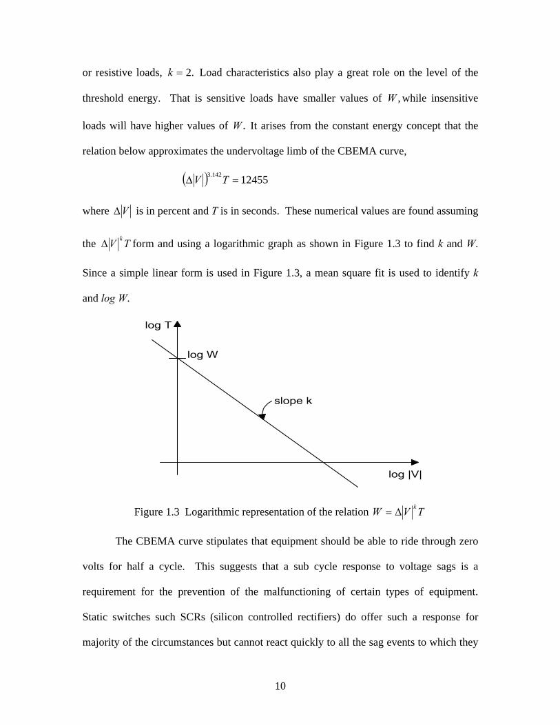
relation below approximates the undervoltage limb of the CBEMA curve,

( ) 12455142.3 =∆ TV

where V∆ is in percent and T is in seconds. These numerical values are found assuming

the TV k∆ form and using a logarithmic graph as shown in Figure 1.3 to find k and W.

Since a simple linear form is used in Figure 1.3, a mean square fit is used to identify k

and log W.

log |V|

log T

log W

slope k

Figure 1.3 Logarithmic representation of the relation TVW k∆=

The CBEMA curve stipulates that equipment should be able to ride through zero

volts for half a cycle. This suggests that a sub cycle response to voltage sags is a

requirement for the prevention of the malfunctioning of certain types of equipment.

Static switches such SCRs (silicon controlled rectifiers) do offer such a response for

majority of the circumstances but cannot react quickly to all the sag events to which they

11

are subjected. Their response is limited by the need to process the voltage and current

information to determine the state of the system [11]. In addition, two types of delays

could be identified, one relates to the finite time to reverse bias the switches and the other

has to do with the detection method employed. A popular detection method is the dqO

transform. The dqO transformation is a phasor transformation that is complex and

requires steady state analysis. The dqO transform is derived from Park’s transformation

for rotating machines. An alternative is to use a purely real transform, which avoids the

requirement of steady state operation. Clarke’s transform is such a transformation [11].

Clarke’s transform of the three phase abc system is of the form,

−

−−

=

c

b

a

VVV

VVV

21

23

21

21

23

21

21

0

01

32

β

α

.

The voltages αV and βV are orthogonal vectors. The single quantity VdqO could be used to

represent the abc system as

22βα VVVdqO += .

Ennis and O’Leary established in [11] that even with the dqO transform detection method

the quarter cycle transfer for SCR is not achievable under all circumstances. This is as a

result of the fact that the transfer time of the switch is dependent on both the distribution

system and the control system variables such as sag point-on-wave, sag depth and the

power factor. It is recommended that a rigorous test schedule that examines these

variables should be part of equipment specification. With the assertion that dqO

transform detection method unachievable under all circumstances the depiction of the

severity of voltage sag event, an objective of this work is very crucial to utilities.

12

To depict the severity of a voltage sag event, a voltage sag index has to be

developed. Several methods has been proposed and developed as a means of qualifying

sag events for the purpose of developing a composite index. In one method [9],

developed by Detroit Edison, qualifying sag has at least one phase of the three-phase

system equal to or below 0.75 per unit. This means that sags with minimum voltage

above 0.75 per unit are not counted. In another method developed by Thallam and Heydt

[1], for sag event to qualify for sag index calculation it must lie between 85% and 10%.

Several methods have been developed and employed in calculating voltage sag

index. The most prominent among them are reviewed below.

• The Detroit Edison sag score method [1,9] is perhaps the first method to be used

by a utility company to index low voltage conditions. The sag score is defined in

terms of the root mean square (RMS) values of the phase voltages Va , Vb and

Vc as

Sag Score .3

1VcVbVa ++

−=

The strength of this method lies in the simplicity of its computation. However the

method does not take into consideration the duration of the sag event, which will

indicate its impact on loads. It must be noted that in this method, the voltage sag

data is aggregated for a 15-minute duration at each location. And if one or two

phases are greater than 1.0 per unit, they are reset to 1.0 per unit. This is the

result of neutral shift. The Detroit Edison sag score does not capture phase

information. Also, apart from a heuristic notion of deviation of phase-neutral

voltage, there is no “scientific” or engineering basis of this score.

13

• System Average RMS (Variation) Frequency Index (SARFIx) [5,8] is one of

several indices which are already being used by utilities to address service quality

issues. SARFIx represents the average number of specified RMS variation

measurements events that occurred over the assessment period per customer

served, where the specified disturbances are those with magnitude less than x for

dips and more than x for swells,

t

ix N

NSARFI ∑= ,

where, x is the RMS voltage threshold, Ni, the number of customers experiencing

short duration voltage deviations with magnitudes above x% for x>100 or below

x% for x<100 due to measurement event i. The parameter Ni represents the

number of customers served from the section of the assessed system. The

advantage of the SARFIx index is that it allows for the assessment of RMS

variations of a specified voltage level. Thus, it is always defined with respect to

the voltage threshold x. For an example, if a utility has customers whose

disturbance susceptibility to voltage sags is below 70% of the nominal supply

voltage, then this disturbance group can be assessed using SARFI70. The shortfall

of this index is that it is applicable for short-duration variations in RMS voltage.

Another problem is that the method does not capture three phase events. Other

indices which are subsets of SARFIx and which assess variations of specified

magnitude and IEEE 1159 duration category are detailed in [5]. A disadvantage

of SARFI is that apart from a statistical account of bus voltage sags, SARFI does

not truly measure energy, power, or any quantitative load disruption.

14

• Thallam and Heydt proposed an index, based on the energy lost during a voltage

sag event [1]. This method called Voltage Sag-Lost Energy index (VLSEI) takes

into consideration the voltage dips in all the three phases and their duration. The

lost energy in a sag event or the energy that was not delivered by the system to the

load during a sag event, W is calculated as

( ) TVW pu14.31−=

where Vpu is the phase voltage magnitude in per unit of the nominal voltage during

a sag event, and T is the sag duration in seconds. The power of the voltage, 3.14

was approximated from the CBEMA curve.

This work develops a voltage sag index that takes in to consideration both

magnitude and duration of a sag event. This index addresses three phase issues and

accounts for both balanced and unbalanced faults.

1.7 Applicable standards

There are many possible causes of voltage sag or swell events in electrical system

including line switching surges, lighting impulses, line to ground faults, unbalanced

single phase loads, high impedance connections and malfunctioning of voltage regulators.

The immunity of sensitive electrical systems to these events is addressed in

ITIC/CBEMA 1996 curve and SEMI F47 standard. Voltage unbalance events are

contained in NEMA MG-1-1988 and ANSI standard C84.1-1989 [7]. Other applicable

standards useful to this work are:

15

1) IEEE 1100, IEEE recommended practice for powering and grounding sensitive

electronic equipment.

2) IEEE 1250, IEEE Guide for service to equipment sensitivity to momentary voltage

disturbances.

3) IEEE 1346, Electric power compatibility with electronic process equipment.

16

Chapter 2

Energy disturbance concept

2.1 Introduction

Different types of electrical equipment behave in different ways under voltage sag

events. The impact of a voltage sag disturbance depends on the sensitivity of the

equipment to voltage sags. Energy disturbance concept is a concept based on the fact that

disturbances to load depend on how much energy is delivered to the load [6]. Two types

of events arise from voltage sag disturbances: an overvoltage and undervoltage event. An

overvoltage event will result if excess energy is delivered to the load during the

disturbance. On the other hand, a shortfall in energy delivered will account for an

undervoltage event. If the cited excess or shortfall in energy is too great, the operation of

the load may be disrupted. The power acceptability curves may be thought of as loci of

constant energy. The energy disturbance concept may be used to model the shape of the

power acceptability curves.

The objective of this chapter is to fully analyze the CBEMA curve based on the

energy disturbance concept. The approach involves studying a line commutated three

phase rectifier load under different loads and conditions. PSpice software is used for

simulation and verification of concepts.

17

2.2 Line commutated three phase rectifier loads

Figure 2.1 depicts a line commutated rectifier. For the purposes of illustrating the

energy disturbance concept, this load is used as an example. Specific values of the

voltage supply and load are used to illustrate the main points. The rectifier receives its

supply from a three phase, 480 V AC supply system. For the purpose of analysis, the

rectifier can be considered to composed of two halves: an upper half and a lower half.

The upper half comprises of the diodes D1, D3 and D5. Diodes D2, D4 and D6 make up

the lower half. The operation of the rectifier depicted in Figure 2.1 is as follows: One of

the diodes D1, D3 and D5 (with high positive voltage at its anode) conducts with the

application of the supply voltage. Similarly, one of the diodes D2, D4 and D6 (with high

negative voltage at its anode) conducts and returns the load current. The sequence of

conduction of the diodes in the upper half of the bridge is D1, D3, D5. Likewise, in the

lower half of the bridge, the sequence is D2, D4, D6. If the load current is assumed to be

continuous at all times, then each diode will conduct for 120° in each half cycle of the AC

waveform, followed by 240° of non conduction. Considering the two halves together,

each diode enters conduction 60° after its predecessor in the sequence D1, D2, D3, D4, D5,

D6. Hence the choice of the numbering scheme of the diodes in Figure 2.1.

When any of the diodes connected with the upper (positive) rail conducts, the

potential of the rail is the corresponding AC line voltage less the forward voltage drops of

the conducting diodes. Also, when any of the diodes connected with the lower (negative)

rail conducts, the potential of the rail will be the corresponding AC line voltage minus the

forward voltage drops of the conducting diodes. The voltage across the load is the

difference between the positive and the negative rail potentials.

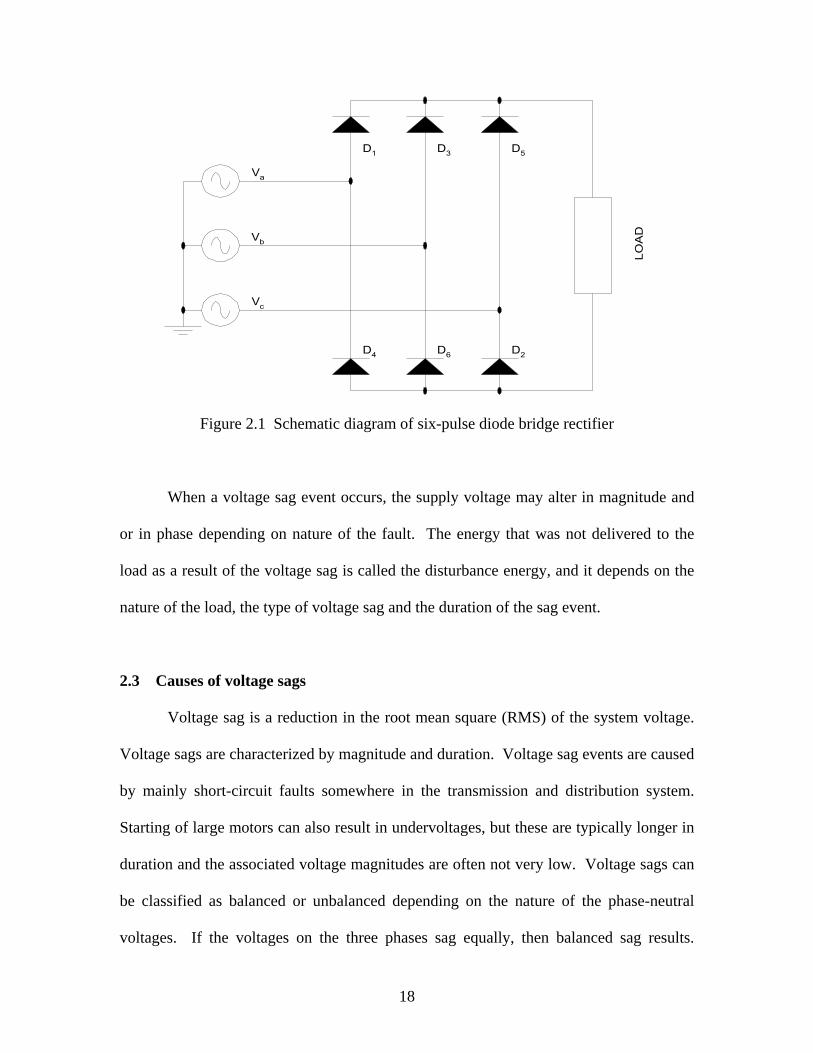
18

D1 D3 D5

D4 D6 D2

Va

Vb

Vc

LOA

D

Figure 2.1 Schematic diagram of six-pulse diode bridge rectifier

When a voltage sag event occurs, the supply voltage may alter in magnitude and

or in phase depending on nature of the fault. The energy that was not delivered to the

load as a result of the voltage sag is called the disturbance energy, and it depends on the

nature of the load, the type of voltage sag and the duration of the sag event.

2.3 Causes of voltage sags

Voltage sag is a reduction in the root mean square (RMS) of the system voltage.

Voltage sags are characterized by magnitude and duration. Voltage sag events are caused

by mainly short-circuit faults somewhere in the transmission and distribution system.

Starting of large motors can also result in undervoltages, but these are typically longer in

duration and the associated voltage magnitudes are often not very low. Voltage sags can

be classified as balanced or unbalanced depending on the nature of the phase-neutral

voltages. If the voltages on the three phases sag equally, then balanced sag results.

19

However, if the phase voltages have unequal voltage magnitudes or phase relationships

other than 120°, the sag is considered as unbalanced.

Three phase short circuits and large motors such as induction motors starting may

cause balanced three phase sags. Unbalanced sags are as a result of lightning, animals,

trees and auto accidents, just to mention a few. Three types of unbalanced voltage sags

could be identified. These are voltage sags resulting from single phase-to-ground faults,

phase-to-phase faults, and phase-to-phase-to-ground faults.

In this chapter the analysis is however restricted to the effect of balanced three

phase faults and unbalanced single phase-to-ground faults on the energy delivered to a

six-pulse bridge rectifier with a pure resistive, inductive and capacitive loads.

2.4 Voltage sag and disturbance energy

During voltage sag, the voltage is below normal for some period of time, which

leads a reduction in the power and the energy delivered to the load. The disturbance

energy is the difference in energy between the actual energy delivered to the load during

the sag duration and the energy that would have been delivered if the load had been

supplied with the normal system voltage over the period. Mathematically, in the case of

a simple resistive load in a DC circuit, the disturbance energy, W may be defined as

TR

VT

RV

W faulteddcrateddc2

,2

, −=

where, Vdc,rated and Vdc,faulted are the rated or the nominal DC voltage and DC voltage as a

result of the voltage sag respectively. For this simple formulation, Vdc,faulted must be

constant. T is the sag duration in seconds and R is the resistance of the load. Of course,

more complex loads (e.g., time varying loads), and AC loads cannot be expressed in this

20

simple way. However, the V2/R type formulation is often found in the literature as a

measure of power irrespective of the load type. In fact, in communications work, the

value R=1 Ω is used thus making the formulation very simple.

The disturbance energy for different load types under different conditions of

voltage sags is simulated for a six-pulse rectifier. The software for the simulation is

PSpice. The simulation involves, setting up two rectifier systems, one to mimic a normal

operation of the rectifier and the other the operation of the rectifier under a voltage sag

event. Nominal three phase voltage system is applied to the rectifiers. After steady state

has been achieved, the supply to one of the rectifiers is disturbed for a period of time.

The energy delivered to the two rectifier systems during the disturbance duration is

recorded. The difference in energy delivered to the two rectifier systems is the

disturbance energy.

The disturbance energy for the different loads connected to the rectifier system

shown in Figure 2.1 under different conditions of voltage sags are summarized for the

cases shown in Table 2.1, and each case is discussed in detail below.

21

Table 2.1 Cases studied for a six-pulse diode bridge rectifier

Conditions

Case AC supply DC load

2.1 Balanced three phase Pure resistive

2.2 Unbalanced (VUF=0.5) Pure resistive

2.3 Balanced (50% sag) Pure resistive

2.4 Unbalanced (phase-to-ground fault) Pure resistive

2.5 Balanced (50% sag) Inductive

2.6 Unbalanced (phase-to-ground fault) Inductive

2.7 Balanced (50% sag) Capacitive

2.8 Unbalanced (phase-to-ground fault) Capacitive

a) Pure resistive load

The schematic circuit diagram for the six-pulse diode bridge rectifier connected

with a pure resistive load is similar to the circuit diagram shown in Figure 2.1, the load

being a pure resistor. The variation of disturbance energy with voltage sag duration for a

pure resistive load is determined for the following types of voltage sags.

• Voltage unbalance factor of 0.5 (Case 2.2)

Voltage unbalance arises in a power distribution system due to incomplete

transposition of transmission lines, unbalanced loads, open delta transformer connections,

open fuses and failed three phase capacitor banks, just to mention a few. The aggravated

effect of the presence of some amounts of unbalance in the line voltages will lead to

22

unproportional unbalance in the line currents [13]. Voltage unbalance factor is defined as

the ratio of the magnitude of the negative sequence component of voltage in the three

phase supply system to the magnitude of the corresponding positive sequence component.

Mathematically, voltage unbalance factor, VUF is given by

VUF= +− VV / .

In this expression, +V and −V are the symmetrical components and

=

−

+

cn

bn

an

VVV

aa

aa

VVV

111

1131

2

2

ο

where .1201 °∠=a Under balanced conditions, .0== −VVο Under any condition,

Parseval’s theorem [4] requires

222οVVVVRMS ++= +− .

For a three phase six-pulse diode bridge rectifier, under unbalanced fundamental supply

voltage conditions, harmonic currents result and therefore harmonic voltages at the

rectifier result. These harmonics occur ideally only in positive and negative sequence.

The presence of the negative sequence components in the fundamental supply voltage

will lead to an overall reduction in the DC voltage at the load. The consequence of this

voltage unbalance is the reduction of the power delivered to the load. The power

reduction is the difference in power between the actual power delivered to the load as a

result of the unbalance in the supply voltage and the power that would have been

delivered in the absence of the voltage unbalance. The percentage power reduction is the

ratio of the cited power reduction to the power delivered to the load in the absence of the

voltage unbalance.

23

Figure 2.2 depicts variation of percentage power reduction for the six-pulse

rectifier with pure resistive load. In this simulation the nominal RMS voltage is kept

constant but the voltage unbalance factor is varied from zero to unity. Harmonic voltages

in the AC supply are not considered. The variation of the disturbance energy with

voltage sag disturbance duration for voltage sag of unbalance factor of 0.5 is shown in

Figure 2.3. The supply voltage, Vac for this example analysis is 480 V RMS and the

value of the DC circuit resistor R is 32.4 Ω.

0

2

4

6

8

10

12

14

16

18

0 0.1 0.2 0.3 0.4 0.5 0.6 0.7 0.8 0.9 1 1.1

Voltage unbalance factor

Perc

ent p

ower

redu

ctio

n to

resi

stiv

e lo

ad

Figure 2.2 Percentage power reduction versus voltage unbalance factor for a six-pulse

diode bridge rectifier with pure resistive load (Case 2.1)

From Figure 2.2 it is evident that an increase in voltage unbalance factor results in

reduction in the power delivered to the load. The percentage reduction in power is

approximately less than 4% when the voltage unbalance factor is less than 0.5. However,

an increase in voltage unbalance factor beyond 0.5 leads to a drastic reduction in the

24

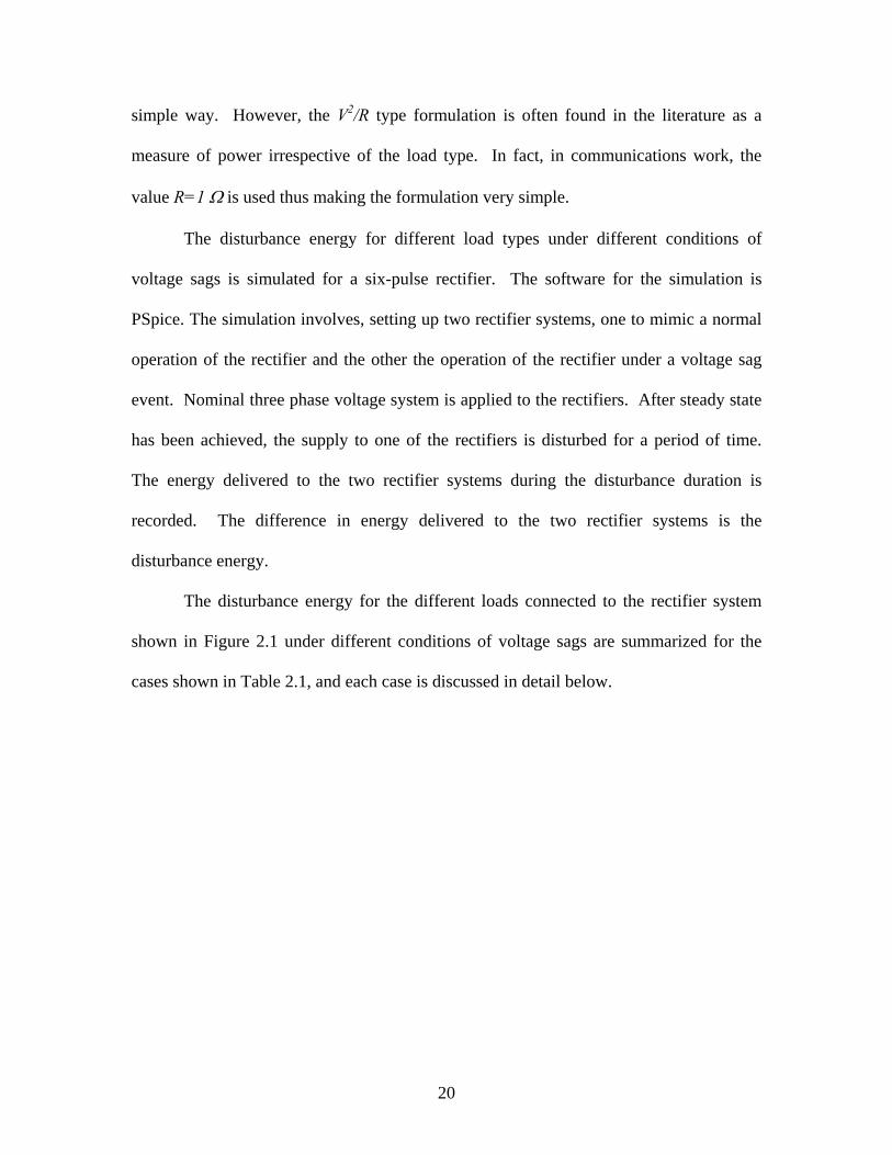
power delivered to the load. Inspection of Figure 2.3 reveals that the disturbance energy

increases linearly with the time duration of the voltage sag for the voltage unbalance

factor of 0.5.

0

20

40

60

80

100

120

140

160

180

0.0 0.1 0.2 0.3 0.4 0.5 0.6 0.7 0.8 0.9 1.0 1.1Disturbance duration in seconds

Dis

turb

ance

ene

rgy

in J

oule

s

Figure 2.3 Disturbance energy for six-pulse diode bridge rectifier with pure

resistive load (voltage sag with unbalance factor of 0.5) (Case 2.2)

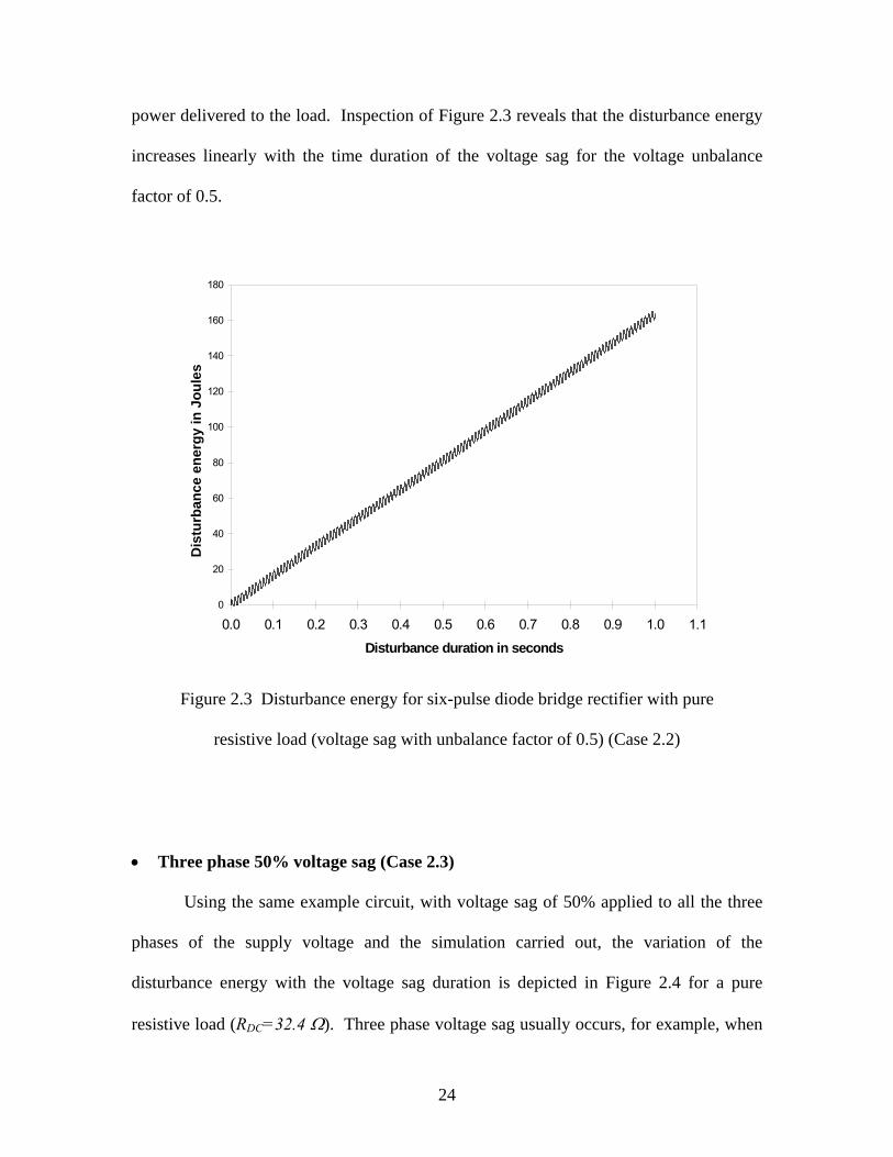
• Three phase 50% voltage sag (Case 2.3)

Using the same example circuit, with voltage sag of 50% applied to all the three

phases of the supply voltage and the simulation carried out, the variation of the

disturbance energy with the voltage sag duration is depicted in Figure 2.4 for a pure

resistive load (RDC=32.4 Ω). Three phase voltage sag usually occurs, for example, when

25

a large induction motor connected to the point of common coupling is started. The

disturbance energy is a simple linear function of disturbance duration in this case.

0

500

1000

1500

2000

2500

0.0 0.1 0.2 0.3 0.4 0.5 0.6 0.7 0.8 0.9 1.0 1.1

Disturbance duration in seconds

Dis

turb

ance

ene

rgy

in J

oule

s

Figure 2.4 Disturbance energy for six-pulse diode bridge rectifier with pure resistive load

(50% three phase voltage sag, Vac=480 V RMS) (Case 2.3)

• Single phase-to-ground fault (Case 2.4)

The large majority of faults on a utility system are single phase-to-ground faults.

Single phase-to-ground faults are unbalanced and usually result from weather conditions

such as lightning. When a single phase-to-ground fault occurs, the voltage on the faulted

phase goes to zero at the fault location. This is simulated by connecting the phase ‘a’ of

the three phase supply to the six-pulse diode bridge rectifier to ground after steady state

26

has been achieved. The disturbance energy versus the voltage sag duration is shown in

Figure 2.5.

0

200

400

600

800

1000

1200

1400

0.0 0.1 0.2 0.3 0.4 0.5 0.6 0.7 0.8 0.9 1.0 1.1

Disturbance duration in seconds

Dis

turb

ance

ene

rgy

in J

oule

s

Figure 2.5 Disturbance energy for six-pulse diode bridge rectifier with pure resistive load

(Phase ‘a’-to-ground fault, Vac=480 V RMS) (Case 2.4)

b) Inductive load

In this study an inductive load in the DC side of a six-pulse rectifier is considered.

The intent is to evaluate the effect of voltage sags on the inductive load by calculating the

disturbance energy through simulation. The schematic circuit diagram for the simulation

is similar to the circuit shown in Figure 2.1. The inductive load consists of a 64.9 H

inductor in series with a 32.4 Ω resistor. The size of the inductor selected ensures that

the load current is constant. Two simulations are performed: a balanced three phase

voltage sag and an unbalanced phase ‘a’-to-ground fault. Figure 2.6 depicts the

27

disturbance energy for six-pulse diode bridge with an inductive load, 50% balanced

voltage sag. The disturbance energy for the case of phase ‘a’-to-ground fault for an

inductive load connected to the six-pulse diode bridge is shown in Figure 2.7.

0

100

200

300

400

500

600

700

0.0 0.1 0.2 0.3 0.4 0.5 0.6 0.7 0.8 0.9 1.0 1.1Disturbance duration in seconds

Dis

turb

ance

ene

rgy

in J

oule

s

Figure 2.6 Disturbance energy for six-pulse diode bridge rectifier with inductive load

(50% voltage sag, Vac=480 V RMS) (Case 2.5)

0

50

100

150

200

250

300

350

400

0.0 0.1 0.2 0.3 0.4 0.5 0.6 0.7 0.8 0.9 1.0 1.1Disturbance duration in seconds

Dis

turb

ance

ene

rgy

in J

oule

s

Figure 2.7 Disturbance energy for six-pulse diode bridge rectifier with inductive load

(Phase ‘a’-to-ground fault, Vac=480 V RMS) (Case 2.6)

28

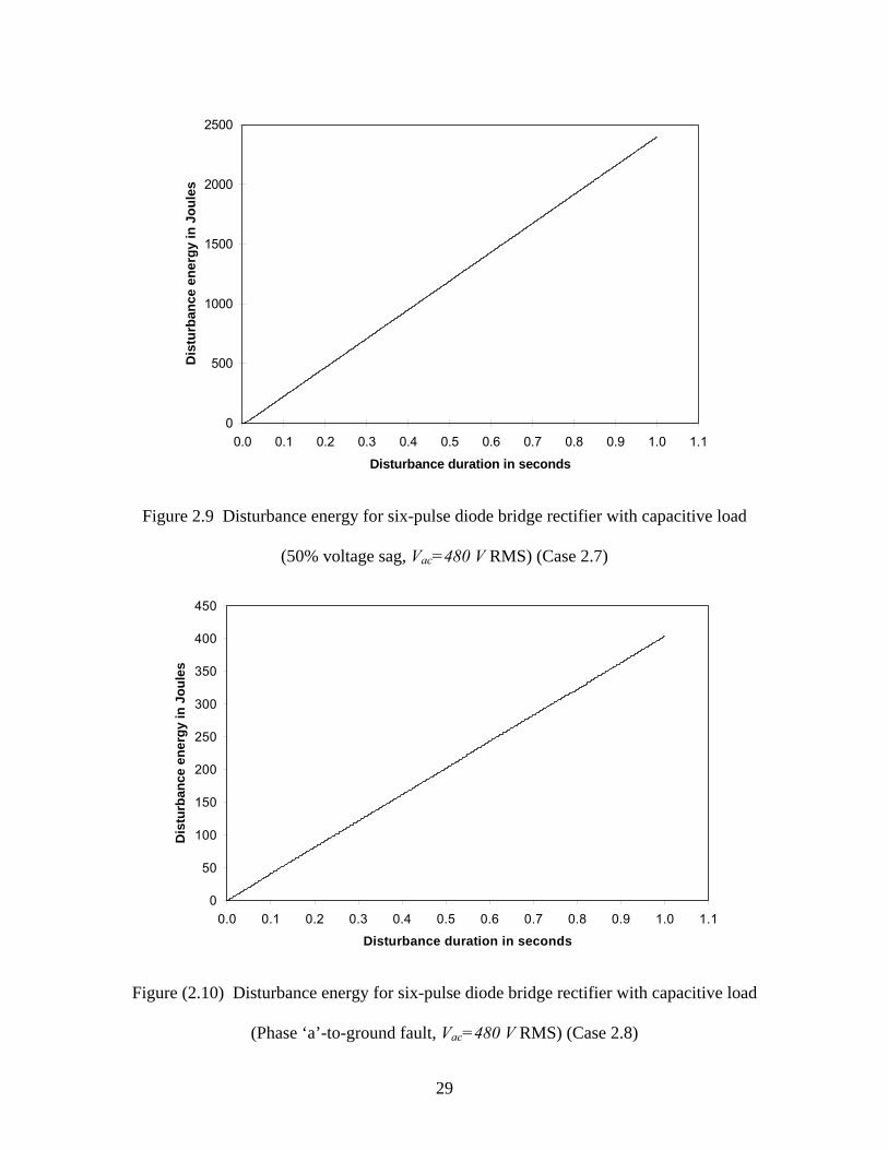
c) Capacitive load

Consider the case of capacitive load in the DC side of the six-pulse rectifier as

depicted in Figure 2.8. The capacitive load comprises of a 10 mF capacitor in parallel

with a 32.4 Ω resistor. The intent, the method and the approach of the simulation are

similar to the one employed in the case of the inductive load. Figures 2.9 and 2.10 are

the disturbance energies for six-pulse diode bridge with capacitive load for the cases of

50% balanced voltage sag and unbalanced phase ‘a’-to-ground fault respectively.

From Figures 2.9 and 2.10 it can be observed that the disturbance energy varies

linearly with the disturbance duration for both the cases of 50% balanced voltage sag and

unbalanced phase ‘a’-to-ground fault. However the impact of the disturbance is severe

when the fault under consideration is a 50% balanced voltage sag.

D1 D3 D5

D4 D6 D2

Va

Vb

Vc

C R

Figure 2.8 Schematic diagram for six-pulse rectifier system with capacitive load

29

0

500

1000

1500

2000

2500

0.0 0.1 0.2 0.3 0.4 0.5 0.6 0.7 0.8 0.9 1.0 1.1Disturbance duration in seconds

Dis

turb

ance

ene

rgy

in J

oule

s

Figure 2.9 Disturbance energy for six-pulse diode bridge rectifier with capacitive load

(50% voltage sag, Vac=480 V RMS) (Case 2.7)

0

50

100

150

200

250

300

350

400

450

0.0 0.1 0.2 0.3 0.4 0.5 0.6 0.7 0.8 0.9 1.0 1.1Disturbance duration in seconds

Dis

turb

ance

ene

rgy

in J

oule

s

Figure (2.10) Disturbance energy for six-pulse diode bridge rectifier with capacitive load

(Phase ‘a’-to-ground fault, Vac=480 V RMS) (Case 2.8)

30

2.5 Disturbance energy and CBEMA curve

In the previous sections the variation of disturbance energy with voltage sags for

different loads were illustrated. In this section, it is intended to find the correlation if any

between the disturbance energy and the CBEMA curve. That is to determine whether

CBEMA is based on disturbance energy concept.

The approach involves calculating disturbance energies for six-pulse diode bridge

rectifier with pure resistive and inductive loads for different three phase voltage sags

through simulation. The simulation is done for a time duration that corresponds to the

threshold sag duration time for the different sag depths on the CBEMA curve. Table 2.2

depicts the threshold disturbance energies for different three phase voltage sag depths for

six-pulse diode bridge rectifier with resistive and inductive loads.

Inspection of Table 2.2 reveals that the threshold disturbance energy for both the

resistive and the inductive loads increase with reduction in the percent voltage sag.

However, one would have expected the threshold disturbance energy to remain constant

with reduction in the percent voltage sag for the stated threshold disturbance durations if

power acceptability curves are to be considered as loci of constant energy. From Table

2.2, CBEMA curve may not be considered, as locus of constant energy and it is therefore

not based on energy.

31

Table 2.2 Threshold disturbance energy for six-pulse diode bridge rectifier with

resistive and inductive loads (balanced three phase sag)

Threshold disturbance energy

(Joules)

Voltage sag

(percent)

Disturbance

duration (seconds) Resistive load

(R=32.4 Ω)

Inductive load

(R=32.4 Ω, L =64.9 H)

-20 1.730 7992.7 4621.6

-25 0.669 2472.7 663.9

-30 0.315 1416.4 239.1

-35 0.213 720.9 66.6

-40 0.100 437.7 25.7

-45 0.057 188.2 5.02

-50 0.042 130.7 2.55

2.6 Summary of the concept of disturbance energy

The concept of disturbance energy has been analyzed, simulated and illustrated

using a three phase line commutated rectifier. It is evident from the simulation results

that disturbance energy is a function of the disturbance duration for all the different load

types considered in the DC circuit of the rectifier.

The following are the salient points that resulted from the simulation and

verification of the concept of disturbance energy:

• The disturbance energy increases with the duration of the sag event. The increase

however depends of the nature of the sag and the load in the DC circuit of the

rectifier. In particular it is realized that for a given sag event and sag duration the

disturbance energy is higher when the load in the DC circuit of the rectifier is

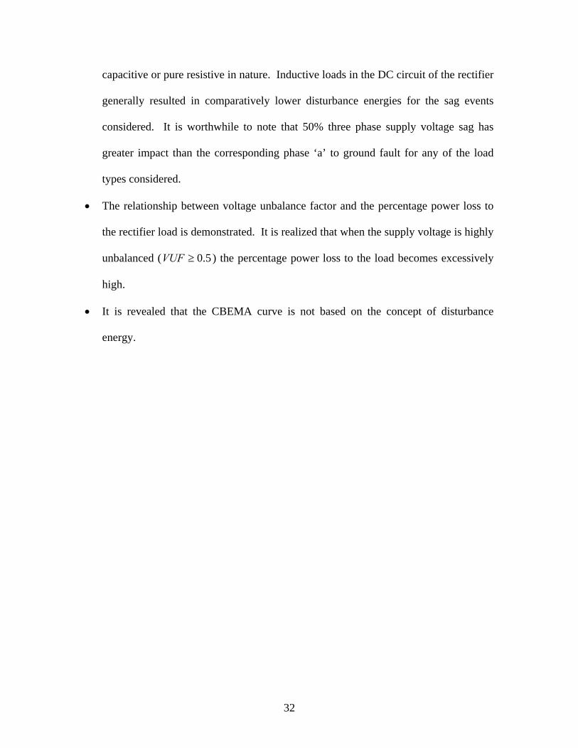
32

capacitive or pure resistive in nature. Inductive loads in the DC circuit of the rectifier

generally resulted in comparatively lower disturbance energies for the sag events

considered. It is worthwhile to note that 50% three phase supply voltage sag has

greater impact than the corresponding phase ‘a’ to ground fault for any of the load

types considered.

• The relationship between voltage unbalance factor and the percentage power loss to

the rectifier load is demonstrated. It is realized that when the supply voltage is highly

unbalanced ( 5.0≥VUF ) the percentage power loss to the load becomes excessively

high.

• It is revealed that the CBEMA curve is not based on the concept of disturbance

energy.

33

Chapter 3

Design of power acceptability curves

3.1 Introduction

The design of power acceptability curves relates to whether the distributed power

can be utilized or not. In other words, the distribution power should be considered

acceptable if the industrial process served is operative. Thus, the ultimate criterion of

power acceptability relates to the operational status of the industrial process. This

criterion depends on the nature of the load. For example, simple incandescent lighting

loads may have a very loose criterion for acceptability, while certain sensitive computer

controls may have a much more restrictive criterion. The difficulty in the selection of a

single criterion is confounded by the many possible load types.

In this chapter, the concept of a power quality standard is introduced and it is used

to construct power acceptability curves for any load type (including the single and three

phase cases) for which the model of the load is known. The majority of this chapter was

also reported in the author’s work in [19].

3.2 The concept of a power quality standard

Power acceptability curves are aides in the determination of the acceptability of

supply voltage to a load or an industrial process. There is no single power acceptability

curve applicable to all loads. However different curves may be designed to capture

different load types and power quality standards. The term 'power quality standard' or

'standard' in short, used in this context refers to the ultimate criterion upon which a

decision of acceptability of supply is made. For an illustration, consider the rectifier load

34

type depicted in Figure 3.1. Voltage sags occurring due to faults in the transmission,

subtransmission, and primary distribution system appear as low voltage condition at Vac

depicted in Figure 3.1. If the sag is of short duration and shallow in depth, the ultimate

industrial process 'rides through' the disturbance. This means that although Vac is

depressed, Vdc does not experience a sufficient disturbance to affect the industrial

process.

Vac

L

C

Lo

ad

Vdc

Figure 3.1 A rectifier load

The concept of power quality standard (voltage standard in this case) is

introduced at this point: a voltage standard is a criterion for power acceptability based on

a minimum acceptable DC voltage at the output of a rectifier below which proper

operation of the load is disrupted. As an example, a voltage standard of 87% for the

rectifier system means that if the Vdc drops below 87% of the rated voltage, the load will

be lost, and the distribution power will be deemed to be unacceptable. The use of the

term 'standard' is however, not meant to imply industry wide standard such as IEEE

standards.

Different loads and industrial processes have different standards. For example, a

rotating load may have a speed standard based on a minimum acceptable shaft speed

below which the industrial process is lost. An electromechanical relay may have a force

35

standard that quantifies the force required to hold a relay armature in a given closed

position. A heating process may have a temperature standard. Each of these standards

entails an ultimate quantity that is related to the AC distribution bus voltage by a

differential equation. The time domain solution of the differential equation yields the ∆V

- T plane locus of the acceptable and unacceptable regions. Thus the concept of a power

quality standard may be used to construct a power acceptability curve for any load type.

3.3 'Derivation' of the CBEMA curve

The CBEMA curve was derived from experimental and historical data taken from

mainframe computers. The best scientific interpretation of the CBEMA curve can be

given in terms of a voltage standard applied to the DC bus voltage of a rectifier load.

Consider the case of either a single phase full wave bridge rectifier or the three

phase bridge counterpart. Let the load on the DC side be an RLC load. If the DC bus

voltage under faulted condition is plotted as a function of the sag duration, the resulting

curve is depicted in Figure 3.2. From Figure 3.2 the locus of Vdc could be represented as

a double exponential in the form,

( ) .ctbtdc CeBeAtV −− ++= (3.1)

Parameter A is the ultimate (t→∞) voltage, Vend, of the rectifier output. For the single

phase case, and for the balanced three phase case, A is simply the depth of the AC bus

voltage sag. For more complex cases, e.g. unbalanced sags, parameter A can similarly be

identified as the ultimate DC circuit voltage if the sag were to persist indefinitely (this is

readily calculable by steady state analysis of the given sag condition and the rectifier

type).

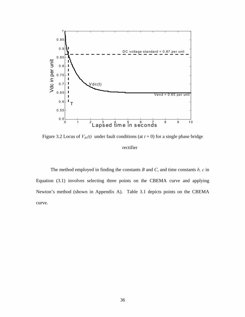
36

0 1 2 3 4 5 6 7 8 9 100.5

0 .55

0 .6

0 .65

0 .7

0 .75

0 .8

0 .85

0 .9

0 .95

1

Laps ed tim e in s ec onds

Vdc

in p

er u

nit

DC vo ltage s tandard = 0 .87 pe r unit

Vend = 0 .65 per unit

V dc(t)

T

Figure 3.2 Locus of Vdc(t) under fault conditions (at t = 0) for a single phase bridge

rectifier

The method employed in finding the constants B and C, and time constants b, c in

Equation (3.1) involves selecting three points on the CBEMA curve and applying

Newton’s method (shown in Appendix A). Table 3.1 depicts points on the CBEMA

curve.

37

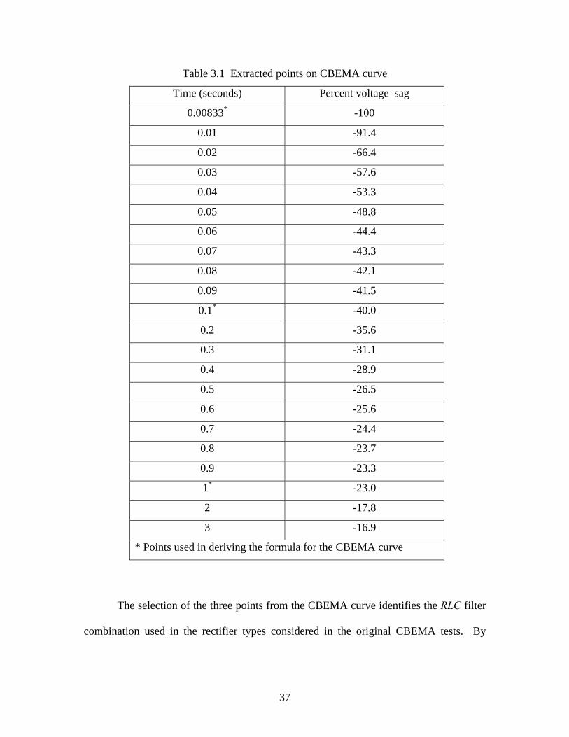
Table 3.1 Extracted points on CBEMA curve

Time (seconds) Percent voltage sag

0.00833* -100

0.01 -91.4

0.02 -66.4

0.03 -57.6

0.04 -53.3

0.05 -48.8

0.06 -44.4

0.07 -43.3

0.08 -42.1

0.09 -41.5

0.1* -40.0

0.2 -35.6

0.3 -31.1

0.4 -28.9

0.5 -26.5

0.6 -25.6

0.7 -24.4

0.8 -23.7

0.9 -23.3

1* -23.0

2 -17.8

3 -16.9

* Points used in deriving the formula for the CBEMA curve

The selection of the three points from the CBEMA curve identifies the RLC filter

combination used in the rectifier types considered in the original CBEMA tests. By

38

substituting the output of the Newton’s method (that is the values of the constants B, C, b

and c), one finds,

Vdc(t)=Vend+0.288e-1.06t+(0.712-Vend)e-23.7t. (3.2)

For the CBEMA curve, let the voltage standard be Vdc ≥ 0.87. Then the Vdc excursion

becomes unacceptable at T when Vdc= 0.87 in Equation (3.2). The solution of Vend in

terms of t= T Equation (3.2) gives

Vend = T

TT

eee

7.23

7.2306.1

1712.0288.087.0

−

−−

−−− .

This is the 'formula' for the undervoltage limb of the CBEMA curve (Vend in per unit, T in

seconds).

3.4 The unbalanced three phase case

Balanced voltage sag events in three phase systems can be treated effectively as a

single phase equivalent. The original CBEMA curve is utilized to address this case.

However, most voltage sags are unbalanced. The voltage sags are as a result of

unbalanced faults such as phase-to-ground, phase-to-phase-to-ground, and phase-to-phase

faults. Perhaps the most common fault type is the phase-to-ground fault in which one of

the phase voltages is depressed.

All the highlighted causes of voltage sag events will have to be considered if one

is to develop a meaningful power acceptability curve for three phase systems. However,

developing a single power acceptability curve to capture all these possible scenarios is

nearly impossible. The approach taken here is one of modeling several fault types in

conjunction with a dynamic load model in order to obtain a power acceptability curve.

39

The ultimate 'standard' is often a DC voltage although speed or other standards may be

used as the load process warrants.

Figure 3.3 shows a power acceptability curve for a three phase rectifier. The case

considered here is that of a phase ‘a’ to ground fault using an 87% Vdc voltage standard.

The procedure for the development of the power acceptability curve is similar to the one

employed in deriving Equation (3.2). The unbalanced fault for the three phase rectifier is

analyzed simply, and Vdc(t) in this case is given as

Vdc(t) = Vend + 0.159e-0.158t + (0.841-Vend)e-4.63t . (3.3)

In Equation (3.3), the time constants were obtained using an LC filter on the DC side of a

three phase, six-pulse bridge rectifier. The values of the LC were chosen to agree with

the filter design used in the single phase case mentioned in conection with the derivation

of Equation (3.2). That is, the CBEMA curve was found to correspond to the single

phase rectifier case plus filter F. If filter F is used as a filter in the three phase case,

Equation (3.3) results. For a voltage standard of

Vdc ≥ 0.87

when substituted into Equation (3.3) gives a formula for the power acceptability curve

shown in Figure 3.3 as

Vend = T

TT

eee

63.4

63.4158.0

1841.0159.087.0

−

−−

−−− .

Power acceptability curve for the case of three phase rectifier with phase-to-phase-to-

ground is shown in Appendix B.

40

10-3 10-2 10-1 100 101 102 103-100

-90

-80

-70

-60

-50

-40

-30

-20

-10

0

Sag duration in seconds

Per

cent

cha

nge

pha

se A

of s

uppl

yvo

ltage

Acceptable power region

Unacceptable power region

Figure 3.3 Power acceptability curve for a three phase rectifier load with a phase-ground

fault at phase ‘a’, 87% Vdc voltage standard

3.5 The speed standard

An important implication of the use of the concept of 'standards' to design power

acceptability curves is that many different industrial processes may be represented. A

rotating load such as induction motor may be thought of to have a standard based on a

minimum acceptable shaft speed, speed standard, below which the operation of the motor

or the industrial process is unacceptable.

The use of the speed standard implies that the industrial process is irreparably

disrupted when the shaft speed of the motor drops below a threshold (e.g., 95% the rated

speed). The problem is complex because of the following issues:

41

• The machine must be modeled under balanced or unbalanced conditions as

appropriate.

• The variation of shaft torque should be modeled. If the threshold shaft speed is near

the rating, the load torque model is not crucial because the shaft torque is nearly

fixed.

• Different machine types and drives may have to be considered.

In this thesis a balanced model of the induction motor is employed for different

variation of load torques but for a speed standard of 95% the rated motor speed.

3.6 Induction motor load representation

For induction motor loads served directly from AC bus, Figure 3.4 applies. The

steady state equivalent circuit from which machine performance can be calculated is

depicted in Figure 3.5. From Figure 3.5, the following electrical and mechanical

equations for the induction motor load can be derived.

a) The slip of the motor, s is given as

s

ssω

ωω −= (3.4)

where ωs and ω are the synchronous and shaft speeds of the machine respectively.

b) The shaft torque, Te is defined in terms of the machine parameter r2 as

s

e srIT

ω2

223= (3.5)

where, I2 is the current flowing the rotor winding at steady state.

c) The differential equation relating the shaft torque and the speed is

Le TBJT ++= ωω& . (3.6)

42

In this expression, TL is the load torque, Bω models viscous friction and J is the shaft

moment of inertia. The solution of the differential equation in Equation (3.6) can be

approximated for small values of t assuming that viscous friction is negligibly small as

( ) tKt ∆+= 0ωω (3.7)

where, K is a constant that depends on the relative magnitudes of Te, TL and J.

Load torque

Shaft speed ω

Frictionaltorque

Vac supply

Moment of inertia

Figure 3.4 Induction machine served from an AC bus

jx1 r1jx2 r2/s

jxmrmV

I2I1

Figure 3.5 Elementary positive sequence induction machine model

43

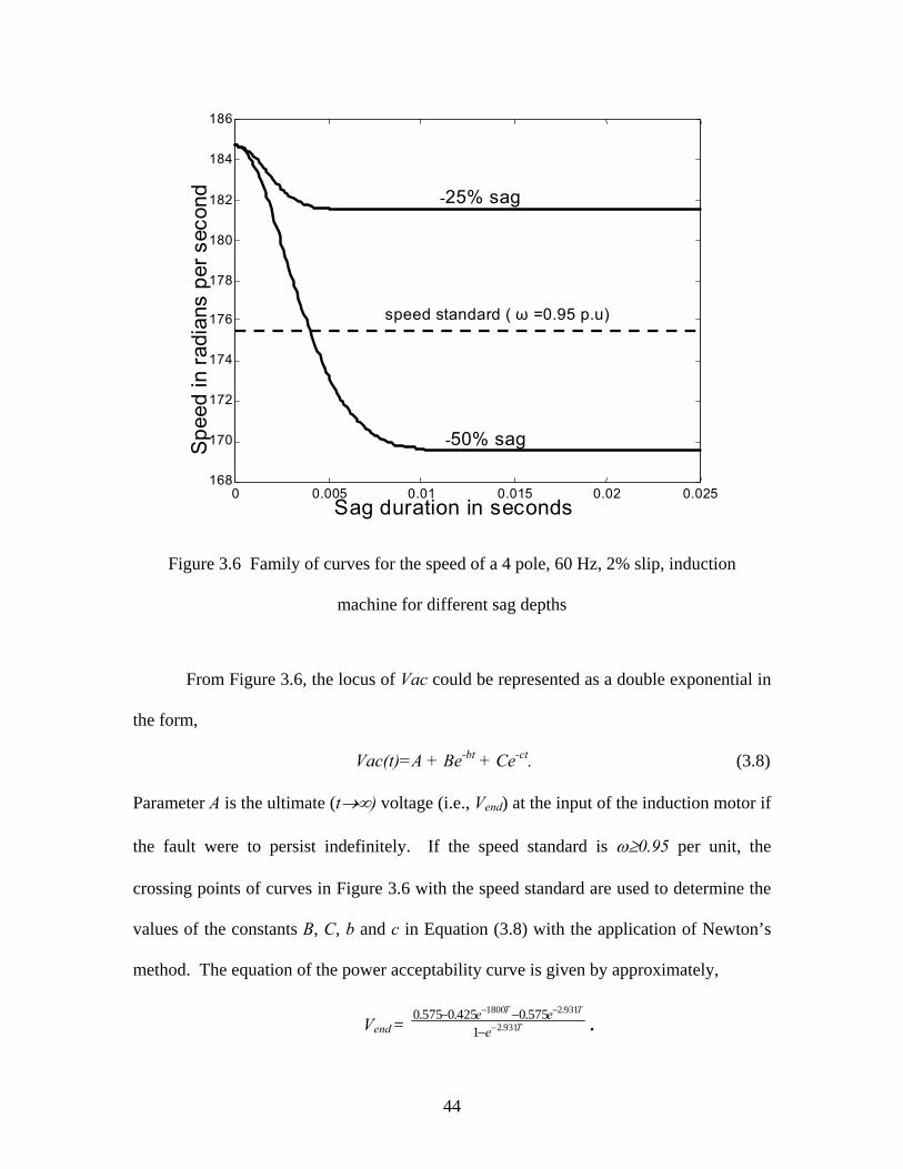
3.7 Pseudocode for the design of a power acceptability curve for an induction

motor load

With an access to the induction motor parameters, the family of curves

corresponding to various sag depths as shown in Figure 3.6 can be obtained through

simulation. The load torque is assumed to be proportional to the shaft speed of the

induction motor. The pseudocode for the simulation is:

Begin

Enter the machine parameters

Initialize t = 0, ω =ωrated

Calculate slip S, torques Te and TL

Calculate shaft speed ω(t) =ω0 + K∆t

While (Te<TL)

Calculate slip S, torques Te and TL

Calculate shaft speed ω(t) =ω0 + K∆t

End while

Plot ω(t)

The complete MATLAB code for the simulation is shown in Appendix C.

44

0 0.005 0.01 0.015 0.02 0.025168

170

172

174

176

178

180

182

184

186

Sag duration in seconds

Spee

d in

radi

ans

per s

econ

d -25% sag

speed standard ( ω =0.95 p.u)

-50% sag

Figure 3.6 Family of curves for the speed of a 4 pole, 60 Hz, 2% slip, induction

machine for different sag depths

From Figure 3.6, the locus of Vac could be represented as a double exponential in

the form,

Vac(t)=A + Be-bt + Ce-ct. (3.8)

Parameter A is the ultimate (t→∞) voltage (i.e., Vend) at the input of the induction motor if

the fault were to persist indefinitely. If the speed standard is ω≥0.95 per unit, the

crossing points of curves in Figure 3.6 with the speed standard are used to determine the

values of the constants B, C, b and c in Equation (3.8) with the application of Newton’s

method. The equation of the power acceptability curve is given by approximately,

Vend = T

TT

eee

931.2

931.21800

1575.0425.0575.0

−

−−

−−−

.

45

The power acceptability curve under the stated conditions for an induction motor load is

shown in Figure 3.7.

10-4 10-3 10-2 10-1 100-100

-90

-80

-70

-60

-50

-40

-30

-20

-10

0

Sag duration in seconds

Per

cent

cha

nge

in s

uppl

y vo

ltage

acceptableoperating region

unacceptableoperating region

Figure 3.7 A power acceptability curve (undervoltage region) for an induction motor

load, speed standard ω > 0.95 per unit, load torque assumed proportional to shaft speed

3.8 Power acceptability curves for other induction motor load types

Induction motors are employed in driving different types of loads in industry and

commercial establishments. The torque characteristics of these loads vary significantly,

from one where the load torque is constant independent of shaft speed to one where the

load torque is proportional to the cube of the shaft speed. The question that one may ask

is, can a single power acceptability curve be applied to any of these possible industrial

and commercial loads? Figure 3.8 depicts the power acceptability curve for the induction

46

motor load, load torque assumed to be constant. The development of this curve is similar

to that shown in Figure 3.7 with the exception that the load torque is constant.

10-4 10-3 10-2 10-1 100-100

-90

-80

-70

-60

-50

-40

-30

-20

-10

0

Sag duration in seconds

Perc

ent c

hang

e in

sup

ply

volta

ge

acceptableoperating region

unacceptableoperating region

Figure 3.8 A power acceptability curve (undervoltage region) for an induction motor

load, speed standard ω > 0.95 per unit, load torque assumed to be constant

The case of induction motor driving a load whose torque characteristics vary as

the square of the motor shaft speed is shown in Figure 3.9. It could be observed from

Figures 3.7, 3.8 and 3.9 that the load driven by the induction motor plays a critical role as

to how susceptible the machine will be to voltage sags. Whereas an induction motor

driving a constant torque load can withstand voltage sag of approximately 60%

indefinitely without tripping, the induction motor driving a load with torque proportional

to the shaft speed can only withstand voltage sag of approximately 42% indefinitely.

47

Thus, one needs to have an idea of the driven load torque characteristics in order to make

an informed decision as to which power acceptability curve to apply. If the induction

motor drives multiple loads of different torque characteristics, one might apply a power

acceptability curve with narrowest acceptable operating region.

10-4

10-3

10-2

10-1

100

-100

-90

-80

-70

-60

-50

-40

-30

-20

-10

0

Sag duration in seconds

Per

cent

cha

nge

in s

uppl

y vo

ltage

acceptableoperating region

unacceptableoperating region

Figure 3.9 A power acceptability curve (undervoltage region) for an induction motor

load, speed standard ω > 0.95 per unit, load torque assumed proportional to the square of

the shaft speed

48

3.9 The force standard

Power line disturbances such as voltage sags may lead to disruption of continuous

processing industries. The industrial equipment responds in different ways to the sag

event. In some cases, the best solution is to protect the equipment from voltage sags with

the use of voltage restorers such as dynamic voltage restorer. In other cases, it may be

economical to protect the susceptible equipment by isolating it from the supply line. AC

contactors are usually employed in the latter option to make and unmake contacts

between the industrial equipment and electrical system for power or control purposes.

The question that one may ask is, are these contactors capable of riding through voltage

sags?

In many industrial processes, rotating machines are controlled by AC contactors.

While the rotating machines often have inertia to ride through voltage sag disturbances,

contactors have been shown to be particularly more susceptible to voltage sags [21]. An

AC contactor can therefore be considered to require a minimum magnetic holding force,

force standard, to maintain the movable contact in a closed position.

In this work, a force standard of 80% the rated magnetic holding force is used to

design power acceptability curves for electromechanical relays such as AC contactor

under voltage sags.

3.10 Modeling of AC contactor

The AC contactor used in the design of the power acceptability curve is as shown

in Figure 3.10. As depicted in Figure 3.10, the contactor coil is modeled as a resistance R

in series with an inductance L. The contactor receives its supply from an AC source and

the coil provides a magnetic force, which offsets the tension in the spring and ultimately

49

causes the electrical contacts to make. The behavior of the contactor under voltage sags

can be understood if one considers the impact of the sags on the current flowing through

the coil. The magnetic force attracting and holding the movable electrical contact in

position varies as the square of the coil current. The magnetic force oscillates and

becomes zero twice every cycle. The magnetic force thus falls below the minimum

holding force required to keep the movable contact in a closed position for a small

interval of time in each cycle, however the mechanical design and the inertial of

contactor allows it to remain in the closed position. The electrical contacts of the

contactor will therefore remain intact during normal operation. The average effective

magnetic force is one-half of the maximum force. During voltage sags the effective

magnetic force will decrease and the contactor will disengage depending on the depth, the

duration of the sag and the point-on-wave where the sag occurs.

LOADVac

R

L

Contactorcoil contacts

Movablecontact

Figure 3.10 Simplified AC contactor model

50

3.11 Design of power acceptability curve for AC contactors

The design process involves simulating a simplified equivalent circuit of the AC

contactor, which consists of a resistor R in series with an inductor L, connected to an AC

supply using Pspice. The values of R and L were selected such that the ratio of the

reactance to the resistance of the contactor coil is comparable with measurement taken

from a typical 60 Hz, 120 V AC contactor. With the assumption that the average

effective magnetic force is proportional to the average of the square of the current

through the contactor coil, the average effective magnetic force required to hold the

movable contactor in a closed position at the rated voltage is estimated. Different

reduced voltages are applied to the AC contactor at steady state and the times required for

the average effective magnetic holding force to fall to 80% of the rated value (i.e. the

force standard) calculated. The simulation is done for the case where the sag event occur

when the instantaneous value of the supply voltage is zero and the one at which the

voltage is at its peak value. The idea is to find out the impact of the point-on-wave where

the sag event occurs on the performance of the AC contactor.

A double exponential equation model is developed for the locus of the different

voltage sags and the times required for the magnetic holding force to reach the force

standard of 80%. The equation describing the undervoltage region of an AC contactor

under voltage sag with sag event occurring at the point-on-wave where the instantaneous

value of the supply voltage is zero is obtained to be approximately

Vend = T

TT

eee

0272.0

0272.06.711

19.01.09.0

−

−−

−−− . (3.9)

The method and the approach used in obtaining Equation (3.9) are similar to the one used

in deriving Equation (3.2). Figure 3.11 is a graphical representation of Equation (3.9).

51

Figure 3.11 depicts power acceptability curve for an AC contactor with point-on-wave

where sag event occurred being zero instantaneous voltage and force standard of 80%.

10-4

10-3

10-2

10-1

100

101

102

-100

-90

-80

-70

-60

-50

-40

-30

-20

-10

0

Disturbance duration in seconds

Perc

ent c

hang

e in

sup

ply

volta

ge

Unacceptable operating region

Acceptableoperating region

Figure 3.11 A power acceptability curve (undervoltage region) for an AC contactor

(point-on-wave where sag occurred= zero instantaneous voltage; force standard= 80%)

For an AC contactor undervoltage sags with point on wave where sag event

occurred being peak of instantaneous voltage and force standard of 80%, Figure 3.12

results. From Figure 3.11 and Figure 3.12 it is evident that point-on-wave where sag

event occurs plays a role as to the ride-through capability of an AC contactor

undervoltage sag. The acceptable operating region of an AC contactor undervoltage sag

where the sag event occurs at zero instantaneous voltage is slightly wider than for the

case where the sag event occurs at peak instantaneous voltage. However, in both cases a

sag event of 10% the rated voltage can be sustained indefinitely.

52

10-4 10-3 10-2 10-1 100 101 102-100

-90

-80

-70

-60

-50

-40

-30

-20

-10

0

Disturbance duration in seconds

Perc

ent c

hang

e in

sup

ply

volta

ge

Unacceptableoperating region

Acceptableoperating region

Figure 3.12 A power acceptability curve (undervoltage region) for an AC contactor

(point-on-wave where sag occurred= peak instantaneous voltage; force standard= 80%)

3.12 Construction of power acceptability curves

Consider a rectifier system operating under a faulted AC voltage supply. Figure

3.13 depicts the DC voltage of the rectifier under the condition of faulting the AC voltage

supply at time t = 0. The equation of this DC voltage response is of the form

Vdc (t)=Vend+Ae-at+Be-bt. (3.10)

At time t = 0,

B=1-Vend –A.

Also, let t = T be the time to reach the threshold value of the DC bus voltage, VT. These,

when substituted into Equation (3.10) result in

( ) .1 bTend

aTendT eAVAeVV −− −−++= (3.11)

53

The voltage sag, ∆V is given as

∆V = Vend - 1. (3.12)

Combining Equations (3.11) and (3.12), the voltage sag, ∆V is obtained as

∆V = ( ) .1

1bT

bTaTT

eeeAV

−

−−

−

−−+ (3.13)

Vdc(p.u)

t

1

VT

Vend

0 T

Figure 3.13 Rectifier load on an AC system, fault occurs at t = 0, DC voltage depicted

Equation (3.13) is the equation of the ∆V - T locus of the undervoltage limb of a

CBEMA-like power acceptability curve. To identify parameters VT, A, a, and b, note the

following: let Tx be the value of the disturbance time T for which a total outage (that is,

∆V = -1.0 per unit) may be tolerated. Then,

-1 = ( )

xbT

xbTxaTT

eeeAV

−

−−

−

−−+

11

.

Eliminating parameter A gives,

54

∆V = ( )

.1

1

bT

xaTbTxaTxbT

TxbT

T

e

eeee

VeV

−

−−−−

−

−

−−−

−+

(3.14)

Equation (3.14) is the equation of a power acceptability undervoltage curve given the DC

standard VT and the two filter time constants a, b.

3.13 Power acceptability for the case of multiple loads

In practical cases, distribution circuits serve many loads. Each load potentially

has its own standard of power acceptability as well as its own dynamic characteristics. A

conservative approach is to define the overall acceptability region as the intersection of

the individual acceptable regions.

As an example, consider three separate rectifier loads, each can tolerate total AC

voltage outage for 1/120 second each with 87% Vdc voltage standard. If three

representative sets of time constants are used in Equation (3.14), Figure 3.14 results. The

intersection of the three acceptable regions is shown as the shaded area in Figure 3.14.

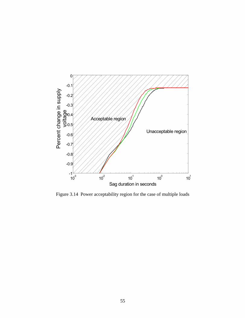
55

10-3

10-2

10-1

100

101

-1

-0.9

-0.8

-0.7

-0.6

-0.5

-0.4

-0.3

-0.2

-0.1

0

Sag duration in seconds

Perc

ent c

hang

e in

sup

ply

volta

ge

Acceptable region

Unacceptable region

Figure 3.14 Power acceptability region for the case of multiple loads

56

Chapter 4

Voltage sag index

4.1 Introduction

Power quality indices often relate to the steady state phenomena, and relatively

few relate to momentary events. However, many power quality engineers feel that bus

voltage sags, a natural consequence of a highly interconnected transmission system, may

be one of the most important type of power quality degradation, and a useful measure of

the severity of these events is desirable. One of such metrics is the power acceptability

curve, which is a graphic metric. The development of a numerical index that measures

the compliance of an event with power acceptability curve is proposed.

A voltage sag index is a parameter that depicts the performance of a power system

with reference to voltage sag. Power acceptability curves such as CBEMA curve (and

the new version ITIC curve) is a magnitude-duration curve, indicating that the severity of

a voltage sag event is a function of both magnitude and duration. In this chapter a

voltage sag index based on the CBEMA technology is proposed. The proposed voltage

sag index, thus employs both the magnitude and time duration information of the sag

event in assessing the acceptability or otherwise of the event.

A graphical comparison of the proposed voltage sag index and other measures of

severity of voltage disturbances such as energy served and sag energy indices are

undertaken.

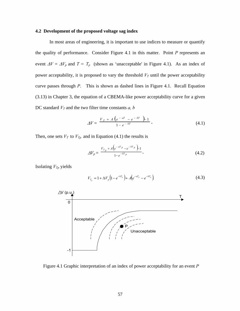
57

4.2 Development of the proposed voltage sag index

In most areas of engineering, it is important to use indices to measure or quantify

the quality of performance. Consider Figure 4.1 in this matter. Point P represents an

event ∆V = ∆Vp and T = Tp (shown as ‘unacceptable' in Figure 4.1). As an index of

power acceptability, it is proposed to vary the threshold VT until the power acceptability

curve passes through P. This is shown as dashed lines in Figure 4.1. Recall Equation

(3.13) in Chapter 3, the equation of a CBEMA-like power acceptability curve for a given

DC standard VT and the two filter time constants a, b

∆V = ( ) .1

1bT

bTaTT

eeeAV

−

−−

−

−−+ (4.1)

Then, one sets VT to VTp and in Equation (4.1) the results is

∆Vp = ( )

.1

1pbT

pbTpaTpT

e

eeAV−

−−

−

−−+ (4.2)

Isolating VTp yields

( ) ( ).11 ppp

p

bTaTbTpT eeAeVV −−− −+−∆+= (4.3)

V (p.u.)

0T

-1

P

Acceptable

Unacceptable

Figure 4.1 Graphic interpretation of an index of power acceptability for an event P

58

Consider the index VTp/VT. If VTp/VT ≥ 1, the point P represents an acceptable

event. It is a simple matter to show that the theoretical maximum of the index VTp / VT is

1/VT. Hence, Figure 4.2 is a graphic depiction of a power acceptability index using the

index Ipa,

Ipa = VTp / VT.

If one uses Tx as in Equation (3.14) in Chapter 3, it is a simple matter to show

Ipa = ( ) ( )( ).111 pp

xaTxbTT

xbTp bTaT

ee

VebTp

T

eeeVV

−−

−

−− −+−∆+ −−

−

(4.4)

This is an index of power acceptability for the event P.

0Ipa

1

Unacceptable Acceptable

1/VT

Figure 4.2 Proposed power acceptability index TTpa VVI

p=

4.3 Correlation of the proposed index to energy served

In the previous section, an index Ipa was proposed based on VTP, a V(t→∞) value

extrapolated from the generalized CBEMA curve,

Ipa = VTP / VT.

As discussed above, if Tpa VI /11 ≤≤ , where VT is the voltage standard (i.e., VT=0.87 per

unit for the CBEMA curve) one concludes that P is an undervoltage event that lies in the

acceptable range on the generalized CBEMA curve. For the standard CBEMA curve

15.11 ≤≤ paI per unit.

59

There are other measures of the severity of a sag event. One such measure is “energy

served” (ES). Energy served refers to the integral of instantaneous power, v(t)i(t), over

an event. In signal processing, the usual assumption of a 1 Ω load is made, from which

one obtains v2(t) as the instantaneous power. Therefore ES is

( ) .0

2 dttvEST

∫=

In the case of actual field measurement, it is not very convenient to calculate this integral

in detail. For this remark, an approximate ES is simply

ES = V2T

Where V is the RMS value of v(t) in Tt <<0 and T is the duration of the event. To form

an index,

TVTVES RMSratedRMSactual ,2

,2=

or on a per unit basis

.,2

RMSactualpu VES =

It is natural to ask the relationship between ES and the voltage sag index, Ipa.

Evidently, as Ipa drops from 1/VT to 1 and further to values smaller than 1; ESpu drops

from 100 percent to lower and lower values. The relationship between ES and Ipa is

discussed further in this section.

The index of power acceptability proposed, Ipa is calculated for a set of voltage

sag events obtained from the field. An empirical comparison of ES and Ipa can be

obtained by examining actual field data. To this end, field data from a primary

distribution system were obtained. The field data, assumed to be exemplary, are shown

in Appendix D. The Ipa for the three phase data is obtained by applying the three phase

voltage set to a six-pulse diode bridge rectifier system. The DC voltage obtained at the

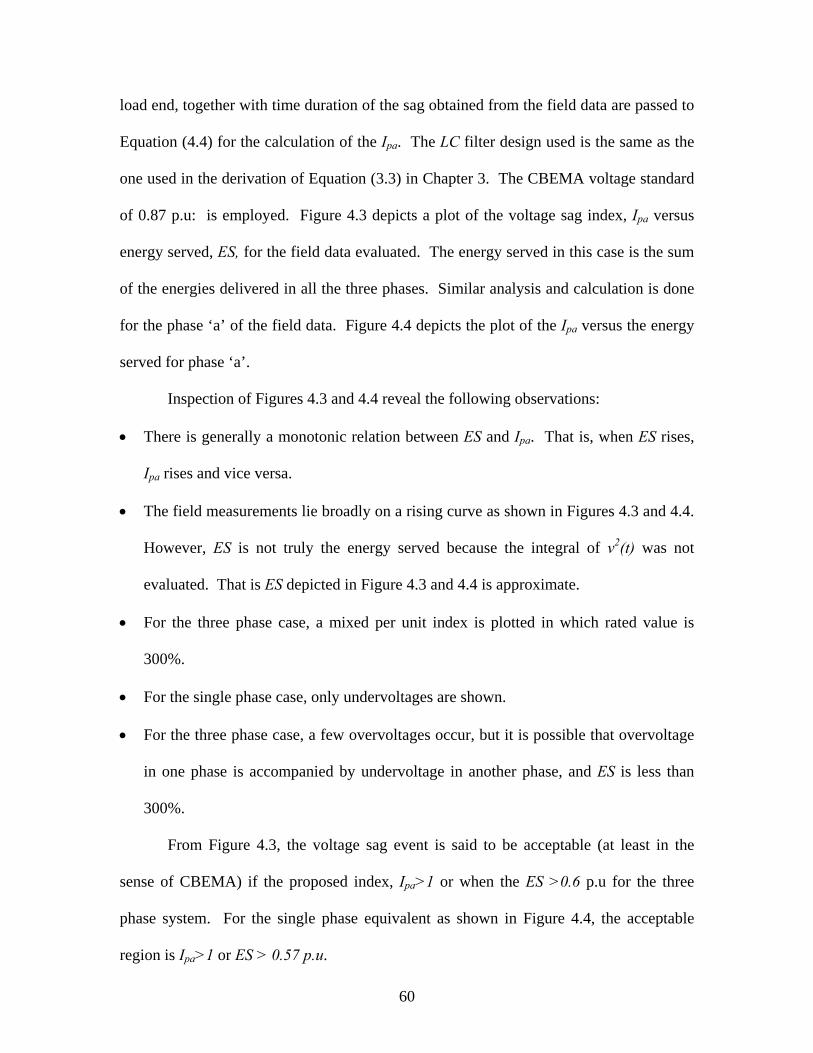
60

load end, together with time duration of the sag obtained from the field data are passed to

Equation (4.4) for the calculation of the Ipa. The LC filter design used is the same as the

one used in the derivation of Equation (3.3) in Chapter 3. The CBEMA voltage standard

of 0.87 p.u: is employed. Figure 4.3 depicts a plot of the voltage sag index, Ipa versus

energy served, ES, for the field data evaluated. The energy served in this case is the sum

of the energies delivered in all the three phases. Similar analysis and calculation is done

for the phase ‘a’ of the field data. Figure 4.4 depicts the plot of the Ipa versus the energy

served for phase ‘a’.

Inspection of Figures 4.3 and 4.4 reveal the following observations:

• There is generally a monotonic relation between ES and Ipa. That is, when ES rises,

Ipa rises and vice versa.

• The field measurements lie broadly on a rising curve as shown in Figures 4.3 and 4.4.

However, ES is not truly the energy served because the integral of v2(t) was not

evaluated. That is ES depicted in Figure 4.3 and 4.4 is approximate.

• For the three phase case, a mixed per unit index is plotted in which rated value is

300%.

• For the single phase case, only undervoltages are shown.

• For the three phase case, a few overvoltages occur, but it is possible that overvoltage

in one phase is accompanied by undervoltage in another phase, and ES is less than

300%.

From Figure 4.3, the voltage sag event is said to be acceptable (at least in the

sense of CBEMA) if the proposed index, Ipa>1 or when the ES >0.6 p.u for the three

phase system. For the single phase equivalent as shown in Figure 4.4, the acceptable

region is Ipa>1 or ES > 0.57 p.u.

61

Now the salient question is, is there any advantage of working with Ipa? The

following are the advantages and the disadvantages of Ipa and ES:

• ES is easier to calculate and instrument.

• Ipa is more theoretically ‘correct’ once CBEMA is accepted.

• Ipa is fully extendable to other criteria (e.g. speed, force criterion), but ES is not.

• The physical meaning of ES is based on energy. Ipa is voltage based

• Three phase implications favor Ipa.

• Sag duration is not captured in ES.

0

20

40

60

80

100

120

140

160

180

200

220

240

260

280

300

0 0.1 0.2 0.3 0.4 0.5 0.6 0.7 0.8 0.9 1 1.1 1.2 1.3

Proposed index, Ipa

Ener

gy s

erve

d in

per

uni

t

Acceptable region (Energy served >0.6 p.u)

Acce

ptab

le re

gion

(Ipa

>1)

Ipa=

1.15

Ove

rvol

tage

'Acceptability' for the purposes of this graph

refers to operation in the lower half-portion of the

CBEMA curve in the acceptable power

region.

Figure 4.3 Proposed index, Ipa versus ES for the three phase system

62

0

10

20

30

40

50

60

70

80

90

100

0 0.2 0.4 0.6 0.8 1 1.2

Proposed index, Ipa

Ener

gy s

erve

d in

per

uni

tAcceptable region (Energy served >0.57 p.u)

Acce

ptab

le re

gion

(Ipa

>1)

Ipa=

1.15

'Acceptability' for the purposes of this graph refers to the operation in the lower half-plane of the CBEMA curve in the acceptable power

region.

Figure 4.4 Proposed index, Ipa versus ES for the phase ‘a’ of the three phase system

4.4 Voltage sag index, Ipa versus sag energy index

In this section, the proposed voltage sag index, Ipa is compared graphically with

another index of power acceptability, sag energy index (SEI), that is presently being used

by a utility company. The intent is to establish if possible the relationship between Ipa

and SEI.

Sag energy index literally represents the sum of voltage sag energies for all events

measured at a given site during a given period. Mathematically, sag energy index is

defined as

SEI = [(100−ESa) + (100−ESb ) + (100−ESc)] × [event duration]

where ESa, ESb, ESc are the phase energy values. The phase energy values are computed

as follows:

63

100_

_

2_

_

_

2_

×=

∫

∫endevent

starteventrateda

endevent

starteventactuala

a

dtV

dtVES

100_

_

2_

_

_

2_

×=

∫

∫endevent

starteventratedb

endevent

starteventactualb

b

dtV

dtVES

100_

_

2_

_

_

2_

×=

∫

∫endevent

starteventratedc

endevent

starteventactualc

c

dtV

dtVES .

These phase energy values are usually measured using electronic monitors in the field.

This is done by subjecting the voltage sag event to 10-minute temporal aggregation. The

most severe event within the 10-minute duration is recorded.

Sag energy index, SEI values are calculated from the field data shown in

Appendix D and it is plotted against the proposed voltage sag index, Ipa. In computing the

SEI values events longer than 60 seconds, overvoltage events and transient events are not

include. Also, voltage sag events longer than 15 cycles are calculated as a 15-cycle

event. Further, phase energy values greater then 100% are limited to a maximum of

100%.

Figure 4.5 depicts a plot of voltage sag index, Ipa versus the values of SEI

evaluated from the field data shown in Appendix D. From Figure 4.5, it is evident that Ipa

and SEI have roughly a polynomial relationship. An acceptable region in the sense of

CBEMA for Ipa is Ipa>1. This region corresponds to SEI <14.

64

0

10

20

30

40

50

60

70

80

0 0.1 0.2 0.3 0.4 0.5 0.6 0.7 0.8 0.9 1 1.1 1.2

Proposed index, Ipa

Sag

ener

gy in

dex,

SEI

SEI=14

Ipa=

1

Figure 4.5 Proposed voltage sag index, Ipa versus SEI for the three phase system

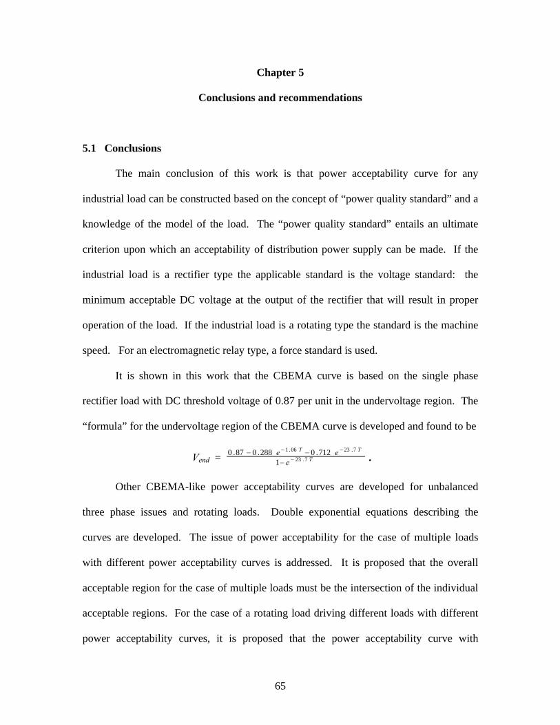
65

Chapter 5

Conclusions and recommendations

5.1 Conclusions

The main conclusion of this work is that power acceptability curve for any

industrial load can be constructed based on the concept of “power quality standard” and a

knowledge of the model of the load. The “power quality standard” entails an ultimate

criterion upon which an acceptability of distribution power supply can be made. If the

industrial load is a rectifier type the applicable standard is the voltage standard: the

minimum acceptable DC voltage at the output of the rectifier that will result in proper

operation of the load. If the industrial load is a rotating type the standard is the machine

speed. For an electromagnetic relay type, a force standard is used.

It is shown in this work that the CBEMA curve is based on the single phase

rectifier load with DC threshold voltage of 0.87 per unit in the undervoltage region. The

“formula” for the undervoltage region of the CBEMA curve is developed and found to be

Vend = T

TT

eee

7.23

7.2306.1

1712.0288.087.0

−

−−

−−− .

Other CBEMA-like power acceptability curves are developed for unbalanced

three phase issues and rotating loads. Double exponential equations describing the

curves are developed. The issue of power acceptability for the case of multiple loads

with different power acceptability curves is addressed. It is proposed that the overall

acceptable region for the case of multiple loads must be the intersection of the individual

acceptable regions. For the case of a rotating load driving different loads with different

power acceptability curves, it is proposed that the power acceptability curve with

66

narrowest acceptable operating region must be applied. The point-on-the wave where a

voltage sag event occurs play a great role in defining the acceptable region for the case of

AC contactor loads.

The analysis of power acceptability curves from the point of view of energy

disturbance concept, an objective of this work is captured. It became clear from the

analysis that the shape of the power acceptability curves cannot be modeled based on the

disturbance energy concept.

An index based on compliance of power acceptability curve is proposed. The proposed

index is a function of voltage sag magnitude and duration since power acceptability curves

are function of both sag magnitude and duration. The proposed voltage index, Ipa is

defined as

Ipa = ( ) ( )( ).111 pp

xaTxbTT

xbTp bTaT

ee

VebTp

T

eeeVV

−−

−

−− −+−∆+ −−

−

Unbalanced and balanced three phase issues are accounted for in the proposed power

acceptability index. The comparisons of the index with other measures of the severity of

voltage sag events are illustrated.

5.2 Recommendations

It is recommended that the proposed method to design power acceptability curves

is extended to other industrial load types that this work failed to address. These include

forced commutated rectifiers, temperature sensors and other protective relays.

After a suitable period of evaluating the proposed method, it may be possible to

use this technique as a recommended practice in industry.

67

References

[1] R. S. Thallam, G.T. Heydt, “Power acceptability and voltage sag indices in the three

phase sense,” Paper presented at Panel Session on “Power Quality-Voltage Sag Indices,”

IEEE PES Summer Meeting, July 2000, Seattle, WA.

[2] R. Waggoner, “Understanding the CBEMA curve,” Electrical Construction and

Maintenance, Vol. 90, No. 10, October 1991, pp. 55-57.

[3] G. Heydt, W. Jewell, “Pitfalls of electric power quality indices,” IEEE Transactions

on Power Delivery, Vol. 13, No. 2, April 1998, pp. 570-578.

[4] G. T. Heydt, Electric Power Quality, Stars in a Circle Publication, Scottsdale, AZ

1995.

[5] D. L. Brooks, R. C. Dugan, M. Waclawiak, A Sundaram, “Indices for assessing utility

distribution systems RMS variation performance,” IEEE Transactions on Power

Delivery, Vol. 131, January 1998, pp. 254-259.

[6] G. T. Heydt, G. G. Karady, B. Cummings, J. Tang, “Improved application of power

acceptability curves and their application to three-phase loads,” Journal of Electric

Machines and Power Systems, July 1999, Vol. 27, pp. 737-751.

68

[7] M. Stephens, J. McComb, “Power quality in chiller systems,” Power Quality

Assurance, September/October 2000, pp. 42-52.

[8] D. D. Sabin, T. E. Grebe, A. Sundaram, “RMS voltage variation statistical analysis

for a survey of distribution system power quality performance,” IEEE Power Engineering

Society 1999 Winter Meeting, Vol. 2, January 1999, pp. 1235-1240.

[9] A. Dettloff, “Power quality performance component of the special manufacturing

contracts between energy provider and customer,” IEEE Power Engineering Society 2000

Summer Meeting, Vol. 2, July 2000, pp. 912.

[10] G. T. Heydt, “Electrical power quality: a tutorial introduction,” IEEE Computer

Applications in Power, Vol. 111, January 1998, pp. 15-19.

[11] M. G. Ennis, R. P. O’Leary, “Solid state transfer switches: the quarter-cycle myth,”

Power Quality Assurance, December 2000, pp. 10-16.

[12] N. S. Tunaboylu, E. R. Collins Jr., S. W. Middlekauff, R. L. Morgan, “Ride-through

issues for DC motor drives during voltage sags,” IEEE Industrial Application Society

Southeast Conference, July 1995, pp. 52-58.

[13] L. Ching-Yin, C. Bin-Kwie, L. Wei-Jen, H. Yen-Feng, “Effects of various

unbalanced voltages on the operation performance of an induction motor under the same

69

voltage unbalance factor condition,” IEEE Industrial and Commercial Power Systems

Technical Conference, July 1997, pp. 51-59.

[14] E. Collins, R. Morgan, “A three phase sag generator for testing industrial

equipment,” IEEE Transactions on Power Delivery, Vol. 11, No. 1, January 1996, pp.

526 - 532.

[15] D. Koval, “Computer performance degradation due to their susceptibility to power

supply disturbances,” Conference Record, IEEE Industry Applications Society Annual

Meeting, October 1989, Vol. 2, pp. 1754 - 1760.

[16] M. Bollen, L. Zhang, "Analysis of voltage tolerance of AC adjustable-speed drives

for three-phase balanced and unbalanced sags," IEEE Transactions on Industry

Applications, Vol. 36, No. 3, May-June 2000, pp. 904 -910.

[17] E. Collins, A. Mansoor, "Effects of voltage sags on AC motor drives," Proceedings

of the IEEE Technical Conference on the Textile, Fiber and Film Industry, May 1997, pp.

9 - 16.

[18] J. C. Gomez, M. M. Morcos, C. Reineri, G. Campetelli, “Induction motor behavior

under short interruptions and voltage sags,” IEEE Power Engineering Review, Vol. 21,

No. 2, February 2001, pp. 11-15.

70

[19] J. Kyei, R. Ayyanar, G. Heydt, R. Thallam, J. Blevins, “The design of power

acceptability curves,” Submitted for publication, IEEE Power Engineering Society, May

2001.

[20] E. R. Collins, Jr., M. A. Bridgwood, “ The impact of power system disturbances on

AC-coil contactors,” IEEE Technical Conference on Textile, Fiber and Film Industry,

June 1997, pp. 2-6.

[21] A. Kelley, J. Cavaroc, J. Ledford, L. Vassalli, “Voltage regulator for contactor ride

through,” IEEE Transactions on Industry Applications, Vol. 36, No. 2, March 2000, pp.

697-703.

[22] M. F. McGranaghan, D. R. Mueller, M. J. Samotyj, “Voltage sags in industrial

systems,” IEEE Transactions on Industrial Applications, Vol. 29, No. 2, March 1993, pp.

397-403.

[23] E. R. Collins, Jr., F. Zapardiel, “An experimental assessment of AC contactor

behavior during voltage sags,” Proceedings of IEEE International Symposium on

Industrial Electronics, Vol. 2, July 1997, pp. 439-444.

[24] J. Kyei, G. Heydt, R. Ayyanar, R. Thallam, J. Blevins, “The design of power

acceptability curves,” Submitted for publication, Northern American Power Symposium,

May 2001.

71

Appendix A

Newton’s method for solving nonlinear system of equations

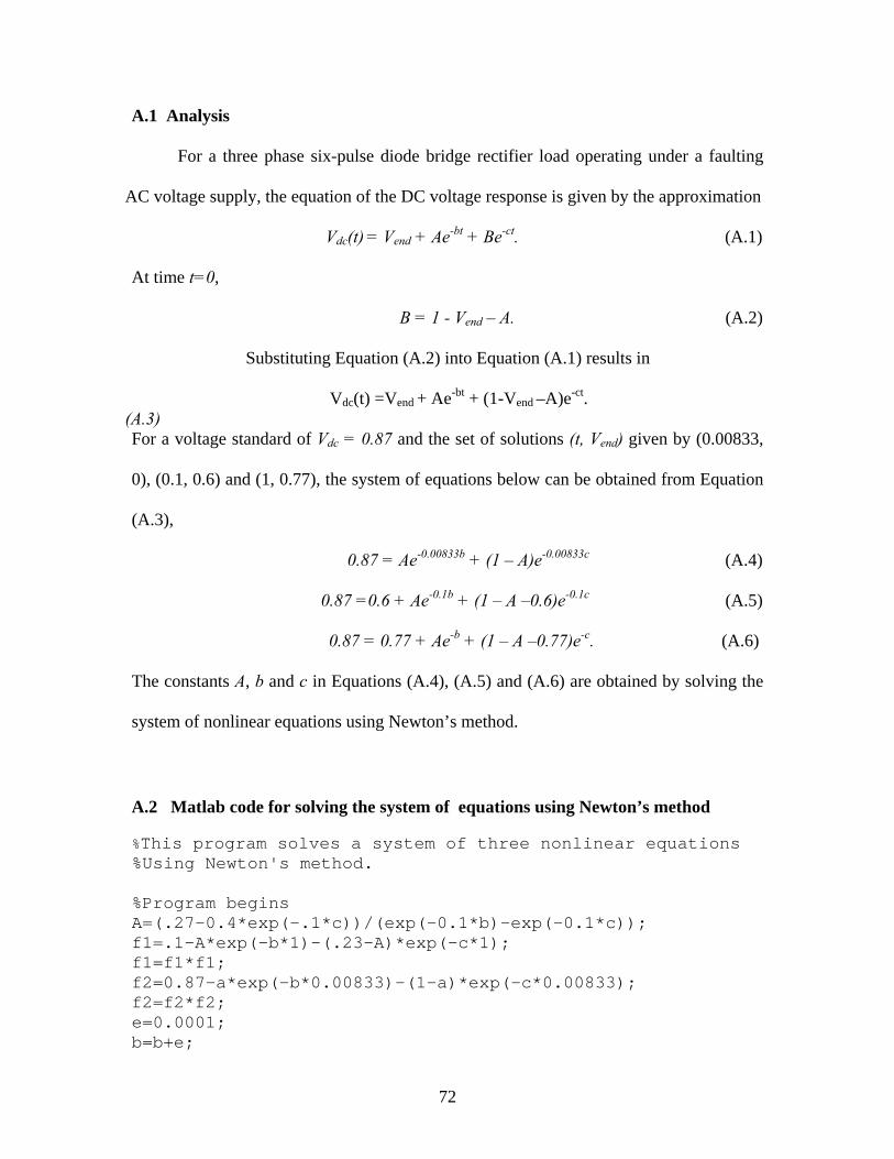
72

A.1 Analysis

For a three phase six-pulse diode bridge rectifier load operating under a faulting

AC voltage supply, the equation of the DC voltage response is given by the approximation

Vdc(t) = Vend + Ae-bt + Be-ct. (A.1)

At time t=0,

B = 1 - Vend – A. (A.2)

Substituting Equation (A.2) into Equation (A.1) results in

Vdc(t) =Vend + Ae-bt + (1-Vend –A)e-ct. (A.3) For a voltage standard of Vdc = 0.87 and the set of solutions (t, Vend) given by (0.00833,

0), (0.1, 0.6) and (1, 0.77), the system of equations below can be obtained from Equation

(A.3),

0.87 = Ae-0.00833b + (1 – A)e-0.00833c (A.4)

0.87 =0.6 + Ae-0.1b + (1 – A –0.6)e-0.1c (A.5)

0.87 = 0.77 + Ae-b + (1 – A –0.77)e-c. (A.6)

The constants A, b and c in Equations (A.4), (A.5) and (A.6) are obtained by solving the

system of nonlinear equations using Newton’s method.

A.2 Matlab code for solving the system of equations using Newton’s method %This program solves a system of three nonlinear equations %Using Newton's method. %Program begins A=(.27-0.4*exp(-.1*c))/(exp(-0.1*b)-exp(-0.1*c)); f1=.1-A*exp(-b*1)-(.23-A)*exp(-c*1); f1=f1*f1; f2=0.87-a*exp(-b*0.00833)-(1-a)*exp(-c*0.00833); f2=f2*f2; e=0.0001; b=b+e;

73

A=(.27-0.4*exp(-0.1*c))/(exp(-0.1*b)-exp(-0.1*c)); f1b=.1-A*exp(-b*1)-(.23-A)*exp(-c*1); f1b=f1b*f1b; f2b=0.87-A*exp(-b*0.00833)-(1-A)*exp(-c*0.00833); f2b=f2b*f2b; b=b-e; c=c+e; A=(.27-0.4*exp(-0.1*c))/(exp(-0.1*b)-exp(-0.1*c)); f1c=.1-A*exp(-b*1)-(.23-A)*exp(-c*1); f1c=f1c*f1c; f2c=0.87-A*exp(-b*0.00833)-(1-A)*exp(-c*0.00833); f2c=f2c*f2c; j=[(f1b-f1)/e, (f1c-f1)/e;(f2b-f2)/e, (f2c-f2)/e]; j=inv(j); c=c-e; bc=[b; c]-j*[f1; f2] f1 f2 b=[1,0]*bc; c=[0,1]*bc; %Program ends

74

Appendix B

Power acceptability curve for three phase rectifier: phase-to-phase-ground fault

75

A three phase six-pulse diode bridge rectifier subjected to a phase-to-phase-

ground fault is simulated and the power acceptability curve for this condition is

constructed. The procedure is the similar to that of the phase-to-ground fault. The

equation of the power acceptability curve is obtained as

.1

75.025.087.025.7

25.785.0

t

tt

end eeeV −

−−

−−−

=

The power acceptability curve for the equation shown above is depicted in Figure B.1.

10-3 10-2 10-1 100 101 102 103-100

-90

-80

-70

-60

-50

-40

-30

-20

-10

0

Sag duration in seconds

Perc

ent c

hang

e ph

ases

A a

nd B

of s

uppl

yvo

ltage

Acceptable power region

Unacceptable region

Figure B.1 Power acceptability curve for a three phase rectifier load with a phase-to-

phase-to-ground fault at phases ‘a’ and ‘b’, 87% Vdc voltage standard

76

Appendix C

Matlab code for the simulation of induction motor load

77

%This program simulates an induction motor load under a three phase fault. % The rating of the motor load is 30hp, 480V, 4 pole, 60Hz and 2% slip. %The load driven in this case is a constant load torque. %Program begins % Program input r1=0.22; % rotor resistance in ohms r2=0.22; % stator resistance in ohms x1=0.34; % rotor reactance in ohms(60Hz) x2=0.37; % stator reactance in ohms(60Hz) xm=50; %core and magnetizing branch reactance in ohms (60Hz) rm=500; % core and magnetizing branch resistance in ohms J=.38; % moment of inertia of the induction motor load Ws=60*pi; % synchronous speed of the induction machine in radians per second W(1)=0.98*Ws; % rated motor shaft speed in radians per second t(1)=0.0; % initial time t0=0.0001; % simulation step size for i=1:1:500; %iteration begins s=(Ws-W(i))/Ws; % motor slip at any time % calculation of stator current a1=(rm*xm^2)/(rm^2+xm^2); a2=(xm*rm^2)/(rm^2+xm^2); b1=r2/s; b2=x2; c1=a1*b1-a2*b2; c2=a1*b2+a2*b1; d1=a1+b1; d2=a2+b2; f1=c1*d1+c2*d2; f2=c2*d1-c1*d2; e1=d1^2+d2^2; g1=f1/e1; g2=f2/e1; h1=g1+r1; h2=g2+x1; k1=sqrt(h1^2+h2^2); if i==1 V=277.1; % rated phase voltage else V=0.5*277.1; % voltage sag end

I1=V/k1; % current flowing in the stator winding I2=(sqrt(a1^2+a2^2)/sqrt(d1^2+d2^2))*I1; %rotor current Te=3*(I2^2)*b1/Ws; % shaft torque

78

if i==1 T=Te; % calculation of load torque end err=T-Te; % torelance if ((i>=5)&(err<=0.00001)) Te=T; end K=(Te-T)/J; %Load torque constant t(i+1)=i*t0; %running time W(i+1)=W(i)+K*t(i+1); %shaft speed updated End % Iteration ends %Program output plot(t,W) xlabel('disturbance duration in seconds') ylabel('speed') title('Induction motor speed curve for voltage sags') grid %Program ends

79

Appendix D

Field measurements from primary power distribution system

80

Data obtained from field measurements of a distribution system are depicted in Tables

D.1. Items shown in Tables D.1 are the average voltage measurements all the three

phases and their associated energy served in percentages. Also indicated is the sag

duration, T in seconds. The energy served ES is defined as

TVTVES RMSratedRMSactual ,2

,2= .

Table D.1 Data obtained from field measurements

Percent average voltage Percent energy servedSag duration

(seconds) Va Vb Vc ESa ESb ESc

0.050 86 98 87 73 96 75

0.084 87 86 97 75 74 95

0.067 93 91 99 86 82 99

0.083 76 96 76 58 93 58

0.083 92 89 93 84 80 87

0.083 98 85 83 96 72 69

0.049 88 99 88 77 98 76

0.068 86 85 98 74 71 96

0.049 93 91 100 86 82 100

0.083 75 96 75 57 93 57

0.066 91 89 95 83 79 89

0.067 97 82 81 94 68 65

0.049 86 98 88 73 96 77

0.083 92 89 93 84 80 86

0.034 86 98 87 75 96 75

0.068 97 88 87 94 77 76

0.067 86 85 98 74 72 96

0.067 93 91 100 86 83 100

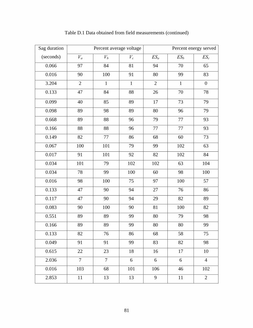
81

Table D.1 Data obtained from field measurements (continued)

Percent average voltage Percent energy servedSag duration

(seconds) Va Vb Vc ESa ESb ESc

0.066 97 84 81 94 70 65

0.016 90 100 91 80 99 83

3.204 2 1 1 2 1 0

0.133 47 84 88 26 70 78

0.099 40 85 89 17 73 79

0.098 89 98 89 80 96 79

0.668 89 88 96 79 77 93

0.166 88 88 96 77 77 93

0.149 82 77 86 68 60 73

0.067 100 101 79 99 102 63

0.017 91 101 92 82 102 84

0.034 101 79 102 102 63 104

0.034 78 99 100 60 98 100

0.016 98 100 75 97 100 57

0.133 47 90 94 27 76 86

0.117 47 90 94 29 82 89

0.083 90 100 90 81 100 82

0.551 89 89 99 80 79 98

0.166 89 89 99 80 80 99

0.133 82 76 86 68 58 75

0.049 91 91 99 83 82 98

0.615 22 23 18 16 17 10

2.036 7 7 6 6 6 4

0.016 103 68 101 106 46 102

2.853 11 13 13 9 11 2

82

Table D.1 Data obtained from field measurements (continued)

Percent average voltage Percent energy servedSag duration

(seconds) Va Vb Vc ESa ESb ESc

0.150 84 96 95 71 92 89

0.067 72 59 97 53 37 95

0.066 73 59 98 55 38 96

0.585 51 40 61 27 17 46

0.066 74 57 98 56 36 96

0.100 89 87 91 79 76 83

0.034 86 98 86 73 97 74

0.099 61 99 98 38 98 97

0.568 56 98 98 31 95 97

0.099 88 86 91 77 75 82

0.034 96 102 93 93 103 86

3.405 0 0 0 0 0 0

68.64 58 59 58 35 35 35

62.09 54 55 54 30 31 31

57.94 54 55 55 31 31 31

18.39 48 48 48 26 26 26

0.016 80 81 81 64 66 65

0.016 85 85 85 71 71 72

0.017 84 84 84 70 71 72

23.24 53 54 54 29 30 30

0.017 72 71 72 52 51 52

1.822 91 92 92 83 85 84

1.97 91 92 92 83 85 84

1.904 91 92 92 83 85 84