1

Analysis and Design of Sub-Harmonically Injection LockedOscillators

Arkosnato Neogy and Jaijeet RoychowdhuryDepartment of Electrical Engineering and Computer Sciences, University of California at Berkeley

Abstract— Sub-harmonic injection locking (SHIL) is an interestingphenomenon in nonlinear oscillators that is useful in RF applications,e.g., for frequency division. Existing techniques for analysis and design ofSHIL are limited to a few specific circuit topologies. We present a generaltechnique for analysing SHIL that applies uniformly to any kind ofoscillator, is highly predictive, and offers novel insights into fundamentalproperties of SHIL that are useful for design. We demonstrate the powerof the technique by applying it to ring and LC oscillators and predictingthe presence or absence of SHIL, the number of distinct locks and theirstability properties, lock range, etc.. We present comparisons with SPICE-level simulations to validate our method’s predictions.

I. INTRODUCTION

Injection locking (IL) [1], [2], [3] is a nonlinear phenomenon in which

a self-sustaining oscillator’s phase becomes precisely locked (i.e.,

entrained or synchronized) to that of an externally applied signal.

The phenomenon, together with the related effect of injection pulling,

has often been regarded as an unwanted disturbance, causing, among

other things, malfunction in serial clock/data recovery, increased

timing jitter and clock skew, increased BER in communications,

etc.. Over the years, however, IL has also been put to good use in

electronics – e.g., for quadrature signal generation [4]; for microwave

generators in laser optics [5]; for fast, low-power frequency dividers

[6]; and in PLLs [7] and wireless sensor networks [8]. Moreover, IL

is an important enabling mechanism in biology (e.g., [9], [10]).

When an oscillator locks to an external signal whose frequency is

close to the oscillator’s natural frequency, the phenomenon is termed

fundamental harmonic IL. It is also possible, however, for oscillators

to phase-lock at a frequency that is an exact integral sub-multiple

of the frequency of the externally applied signal; this is termed sub-

harmonic IL (or SHIL, described further in Sec. II-B) and is useful

in frequency division applications [6], [7].

Design of circuits exploiting SHIL has tended to rely predominantly

on trial-and-error based methodologies, using brute-force transient

simulations to assess impact on SHIL-based circuit function. Exist-

ing analyses of fundamental and sub-harmonic IL (e.g., [11], [2],

[12]) have been limited to very specific circuit topologies (e.g., LC

oscillators), while more general analyses [13], that apply to any kind

of oscillator, do not consider SHIL. The work of Daryoush et. al. [14]

presented a computationally complicated method limited to negative

feedback oscillators, and provided no insights about multiple lock

states for SHIL. To our knowledge, there is no general analysis or

theory that provides the correct design intuition and predictive power

for SHIL and related phenomena.

In this paper, we develop and validate a general method for analysing

and understanding sub-harmonic injection locking. The method ap-

plies to any self-sustaining, amplitude-stable oscillator, not only from

electronics but also from other domains such as biology. Specifically,

we obtain a simple equation that not only has numerical uses for

fast simulation of sub-harmonic injection pulling and locking, but

can be depicted graphically, thereby offering powerful insights into

qualitative and quantitative properties of SHIL in oscillators. One

important such insight is that mth-sub-harmonic locking is intimately

related to the mth-harmonic component of the PPV function [15],

[16], [17] (see Sec. II-A); our analysis provides quantitative design

guidelines for inducing mth-sub-harmonic locking. Another important

insight is that mth-sub-harmonic locking typically occurs in one of 2m

distinct phases (relative to a reference signal at the same frequency);

m of these solutions, spaced uniformly in phase increments of 2πm ,

are dynamically stable.

Development of our method starts from a scalar, non-linear equation

(the PPV equation [15], [16], [17], described further in Sec. II-A) that

governs the phase dynamics of oscillators. We devise a specialized

analysis of the PPV equation by first recasting it in terms of a phase

error metric that detects SHIL, then averaging out fast variations1

to obtain a simple scalar differential equation in the phase error

metric. “DC” analysis of this equation captures SHIL and provides

the insights noted above. A key quantity needed in these equations,

the PPV function specific to a given oscillator, is obtained via efficient

and robust numerical methods [17].

We present extensive numerical experiments that compare detailed

SPICE-level simulations with our new SHIL analysis and validate

its accuracy and predictive nature. Using ring and LC oscillators as

examples, we apply our technique to determine whether or not SHIL

can occur in a given design, in how many distinct ways lock can

occur, how robust a lock is, how an existing design can be modified

to better induce SHIL, etc.. We also prove the existence of multiple

distinct locks using detailed SPICE-level simulations.

The remainder of the paper is organized as follows. Sec. II provides

brief background on PPV phase equations and basic concepts of sub-

harmonic IL. Sec. III-A presents our new analysis of SHIL, while

Sec. III-B discusses key uses and insights that stem from this analysis.

Sec. IV presents numerical experiments on ring and LC oscillators

that validate our approach.

II. PRELIMINARIES

A. The PPV Nonlinear Phase Equation for Oscillators

A SPICE-level representation of any circuit (including oscillators) is

equivalent [18] to a system of differential-algebraic equations (DAEs)

[19] in the form:

d

dt~q(~x(t))+~f (~x)+~b(t) =~0, (1)

where ~x denotes internal state, ~f (·) and ~q(·) capture static and dy-

namic terms, respectively, and~b(t) denotes inputs to the system. Self-

sustaining autonomous oscillators, by their nature, produce periodic,

time-varying solutions ~x(t) even when ~b(t) vanishes (or is constant

with time) — this is termed natural oscillation. Denote such natural

oscillation by ~xs(t) and its period by T . For a large class of self-

sustaining oscillators, it has been shown [16] that if natural oscillation

is disturbed by small time-varying external inputs~b(t), the oscillator’s

response can be approximated well as

~x(t)≃~xs(t +α(t)), (2)

where α(t), a time shift caused by the external inputs, is governed

by the scalar differential equation

d

dtα(t) =~vT

1 (t +α(t)) ·~b(t). (3)

In (3), the vector ~v1(t), known as the Phase Response Curve (PRC)

[15] or Perturbation Projection Vector (PPV) [17], is a T -periodic

1in a manner similar to that used to derive Adler’s equation for fundamentalharmonic IL [1], [13].

2

vector function of time. For the purposes of this paper, we rewrite

(3) by defining a 1-periodic version of the PPV, i.e.,

~p(t) =~v1(Tt), (4)

and using this in (3) to obtain

d

dtα(t) = ~pT ( f t + f α(t)) ·~b(t), (5)

where f , 1T . (5), known as the PPV equation or the PPV phase

macromodel, is the starting point for our SHIL analysis in Sec. III-A.

B. Basic Concepts of Sub-harmonic Phase Locking

Given any T periodic function s(t), if another function r(t) is derived

from it as r(t), s(φ(t)), then φ(t) is termed the phase of r(t) with

respect to the base period T 2. For example, if s(t) is the 1-periodic

sinusoid s(t) = sin(2πt) and

REF(t), s( f0t), (6)

then the phase of REF(t) with respect to the base period 1 is

φREF(t), f0t. (7)

Suppose we are given another signal y(t) with phase φy(t) (with

respect to the same base period as REF(t)). Then REF(t) is said to

in “simple mth sub-harmonic phase lock” to y(t) if

φREF(t) =φy(t)

m+ const. (8)

For example, if y(t), cos(2π ·3 · f0t +0.5), then φREF(t) in (6) is in

simple 3rd sub-harmonic phase lock to y(t).We now establish terminology that will be used in the remainder of

the paper. The natural period of any oscillator will be denoted by T ;

its natural frequency, 1T , will be denoted by f . External inputs to the

oscillator will be denoted by# �

SYNC(t), with frequency fin and phase

φin(t) = fint; i.e., ~b(t) in (1) is given by

~b(t) =# �

SYNC(t) =~c(

φin(t))

, (9)

where ~c(t),~b( tfin) is 1-periodic.

If ~b(t) =# �

SYNC(t) results in mth sub-harmonic lock, then fin ∼ m f ;

define ∆ f by fin = m( f +∆ f ). Denote the frequency of mth sub-

harmonic lock to# �

SYNC(t) by f0; i.e., f0 = fin

m = f +∆ f . Finally,

denote REF(t) to be a reference signal, at frequency f0, that is in

mth sub-harmonic phase lock to the external input signal# �

SYNC(t).

III. ANALYSING THE PPV EQUATION TO CAPTURE SHIL

A. Derivation of the Alderized SHIL equation

We now proceed to analyse SHIL by expressing the PPV equation

(5) equation in terms of phase. We assume that the external input~b(t) equals the

# �

SYNC(t) signal defined in Sec. II-B, with frequency

fin = m f0 and phase φin(t) = fint.

From (2), observe that the phase of the oscillator’s response under ex-

ternal perturbation is φ(t), f t + f α(t). Rewriting the PPV equation

(5) in terms of φ(t), we obtain

d

dtφ(t) = f + f~pT (φ(t)) ·~c(φin(t)). (10)

Define the mth-SHIL phase error to be

θ(t), φ(t)−1

mφin(t). (11)

This definition is motivated by the fact that if the oscillator achieves

simple mth sub-harmonic phase lock to its external input# �

SY NC(t),

2For convenience, we will omit “with respect to ...” when the base periodis implicitly understood (e.g., it is usually 1 in this paper).

then θ(t) ≡ constant. Taking the time-derivative of (11) and using

(10) and the definition of φin(t) from Sec. II-B, we obtain

θ̇(t) = ( f −1

mfin)+ f

(

~pT(

θ(t)+1

mfint

)

·~c( fint))

. (12)

Now, ~p(·) is a 1-periodic function, hence ~p(

θ(t)+ 1m fint

)

may be

expressed using Fourier series as

~p

(

θ(t)+1

mfint

)

=∞

∑k=−∞

~pke j2πk(θ(t)+ 1m

fint), (13)

where {~pk} are the Fourier coefficients3 of ~p(t). Similarly,~c(t) being

a 1-periodic function, we have

~c( fint) =∞

∑l=−∞

~clej2πl fint , (14)

with {~ck} being the Fourier coefficients of ~c(t). Using (13) and (14)

in (12), we arrive at

θ̇(t) =

(

f −1

mfin

)

+ f∞

∑k,l=−∞

~pk ·~clej2π( fint(l+ k

m )+kθ(t)). (15)

The double summation term in (15) contains fast-varying components

(stemming from non-zero coefficients of fint in the exponential), to-

gether with potentially slowly varying components resulting from the

kθ(t) terms. This equation can be simplified under the assumptions

that 1) θ(t) is slowly-varying with respect to time-scales of the order

of mfin

, and 2) ~pT (·) is smooth, i.e., it does not feature large changes

over any argument interval of length ≪ 1. Defining Tin =1fin

and

θa(t),1

mTin

∫ t+mTin

2

t−mTin

2

θ(τ)dτ, (16)

it is easily shown under the above assumptions that

θ̇a(t) =

(

f −1

mfin

)

+ f∞

∑l=−∞

~p−ml ·~cle− j2πmlθa(t). (17)

If the oscillator achieves simple mth sub-harmonic phase lock, then,

as noted earlier, θ(t) ≡ θa(t) ≡ constant, i.e., θ̇(t) ≡ 0; hence (17)

reduces to

fin −m f

m f= g(θ),

∞

∑l=−∞

~p−ml ·~cle− j2πmlθ . (18)

(18), dubbed the Adlerized4 SHIL equation, is a simple scalar

algebraic equation in the SHIL phase error θ , solutions to which

determine whether or not mth sub-harmonic phase lock is possible.

Observe that the LHS of (18) is a constant equalling∆ ff , while its

RHS g(θ) is a real periodic function with period 1m . (18) can easily

be plotted graphically; for example, as in Fig. 2(d) and Fig. 5(d),

discussed further in Sec. IV. The significance of (18), and the insights

it provides into SHIL, are discussed in the next section.

B. Insights resulting from the Adlerized SHIL equation

The simplicity of the form of equation (18) allows several interesting

and useful design insights to be deduced from it. Typically, circuit de-

signers are interested in design variables such as injection amplitude,

lock range, stability of lock, etc., regarding which (18) provides useful

qualitative and quantitative information. (18) also provides additional

insights into the very mechanisms of lock, which translate into key

guidelines for designing oscillators for SHIL.

1) Number, stability and spacing of distinct sub-harmonic locks:

From the facts that the RHS of (18), g(θ), is continuous,

3Given the differential equations (1) of any oscillator, robust and scalablenumerical methods for finding {~pk} are available and well established [17].

4The form of (18) is similar to the well-known Adler equation [1] forfundamental-harmonic injection locking in negative resistance LC oscillators.

3

bounded, differentiable and 1m -periodic, it can be easily proved5

that the number of distinct solutions of (18) is an integral

multiple of 2m – i.e., (18) can have zero, 2m, 4m, etc. solutions

in interval θ ∈ [0,1). There will be no solutions if the value of

the LHS of (18) falls outside the range of g(θ); this indicates

that mth sub-harmonic phase lock is not possible – as depicted in

Fig. 9(b), discussed in Sec. IV. When the LHS does fall within

the range of g(θ), 2m× k solutions can exist – the typical case

being k = 1 or 2m solutions, depicted in Fig. 2(d) and Fig. 5(d).

Moreover, it can be shown that exactly half the solutions are

dynamically stable, with the other half being unstable; indeed,

stable and unstable solutions occur alternately. The separation be-

tween successive stable solutions (and between successive unstable

solutions) is always 1m ; however, the gaps in phase between a

stable solution and its two neighbouring unstable solutions can be

(and typically are) asymmetric. Fig. 2(d) and Fig. 5(d) illustrate

these facts.

The fact that there are multiple stable solutions spaced at phase

differences of 1m increases the possibility that disturbances will

lead to small phase slips when m > 1, compared to fundamental

IL situations where m = 1, potentially leading to increased jitter

concerns during design. Moreover, because of the asymmetric

spacing of neighbouring unstable solutions, the magnitude of the

phase disturbance needed to induce a phase slip depends on

whether its sign is positive or negative. To assess lock robustness,

the lesser of the gaps from a stable lock to its neighbouring

unstable locks should considered during design.

2) The mth harmonic of the PPV enables mth sub-harmonic lock:

From the definition (18) of g(θ), observe that the coefficient of

the lth harmonic component of g(θ) is ~p−ml ·~cl . This shows

that the strength of the mth harmonic component of the PPV is

of key importance in enabling mth harmonic SHIL. For example,

if the second harmonic component of the PPV is much smaller

than its first and third harmonic components (as in Fig. 7(c),

for the symmetric ring oscillator example of Sec. IV-B), then

the oscillator is much more susceptible to first- and third-sub-

harmonic IL than to second-sub-harmonic IL, for external inputs

of the same magnitude. To make it better suited for second

sub-harmonic locking (for example), the oscillator’s design needs

to be changed such that its PPV’s second harmonic component is

accentuated. This can be achieved, for example, by resizing the

transistors in the oscillator’s inverters to make them asymmetric

as in Sec. IV-A1, resulting in the new PPV harmonics shown

in Fig. 2(c). Note also that the presence of higher harmonics

in the input, together with corresponding harmonics in the

oscillator’s PPV, facilitate mth sub-harmonic lock – indicating

that nonlinearity is useful for SHIL. Thus, the Adlerized SHIL

equation (18), together with computational tools for determining

the PPV’s harmonics [17], provides concrete design guidelines

for utilizing SHIL.

3) Analytical lock range formulæ for sinusoidal inputs: When the

injected signal is purely sinusoidal (i.e.,~ck ≡~0,∀k 6=±1), as it can

be in applications, g(θ) becomes purely sinusoidal too, enabling

simple analytical formulæ to be derived that express the SHIL

lock range∆ ff in terms of injection amplitude, and vice-versa6.

The relationship stands as

fin −m f

m f=

1

2·Pm ·C · cos(2πmθ) (19)

where Pm denotes the real magnitude of the mth harmonic com-

ponent of the PPV and C denotes the amplitude of the purely

sinusiodal injected signal. (19) is derived by simplifying the RHS

of (18) using l =±1 only.

5The proof is omitted in the interest of brevity.6Similar to formulæ for fundamental harmonic IL [20].

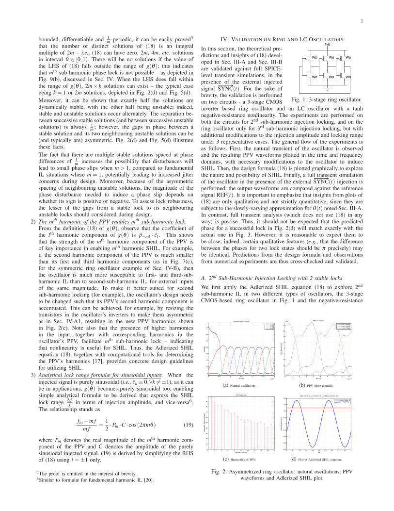
IV. VALIDATION ON RING AND LC OSCILLATORSVdd

Wn

Wp Wp Wp

Wn Wn

Fig. 1: 3-stage ring oscillator.

In this section, the theoretical pre-

dictions and insights of (18) devel-

oped in Sec. III-A and Sec. III-B

are validated against full SPICE-

level transient simulations, in the

presence of the external injected

signal# �

SYNC(t). For the sake of

brevity, the validation is performed

on two circuits - a 3-stage CMOS

inverter based ring oscillator and an LC oscillator with a tanh

negative-resistance nonlinearity. The experiments are performed on

both the circuits for 2nd sub-harmonic injection locking, and on the

ring oscillator only for 3rd sub-harmonic injection locking, but with

additional modifications to the injection amplitude and locking range

under 3 representative cases. The general flow of the experiments is

as follows. First, the natural transient of the oscillator is observed

and the resulting PPV waveforms plotted in the time and frequency

domains, with necessary modifications to the oscillator to induce

SHIL. Then, the design formula (18) is plotted graphically to explore

the nature and possibility of SHIL. Finally, a full transient simulation

of the oscillator in the presence of the external# �

SYNC(t) injection is

performed; the output waveforms are compared against the reference

signal REF(t). It is important to emphasize that insights from plots of

(18) are only qualitative and not strictly quantitative, since they are

subject to the slowly-varying approximation for θ(t) noted Sec. III-A.

In contrast, full transient analysis (which does not use (18) in any

way) is precise. Thus, it should not be expected that the predicted

phase for a successful lock in Fig. 2(d) will match exactly with the

actual one in Fig. 3. However, it is reasonable to expect them to

be close; indeed, certain qualitative features (e.g., that the difference

between the phases for two lock states should be π precisely) may

be identical. Predictions from the design formula and observations

from numerical experiments are thus cross-checked and validated.

A. 2nd Sub-Harmonic Injection Locking with 2 stable locks

We first apply the Adlerized SHIL equation (18) to explore 2nd

sub-harmonic IL in two different types of oscillators, the 3-stage

CMOS-based ring oscillator in Fig. 1 and the negative-resistance

0 0.5 1 1.5 2 2.5 3

x 10−11

0

0.1

0.2

0.3

0.4

0.5

0.6

0.7

time (s)

outp

ut(s

)

transient without forcing

inv1inv2inv3

(a) Natural oscillations.

0 1 2 3 4 5 6 7 8 9

x 10−12

−4

−2

0

2

4

6

8

10

12

x 104

time (s)

PP

V w

avef

orm

(s)

PPV waveforms

inv1 (HBadj)inv2 (HBadj)inv3 (HBadj)

(b) PPV (time domain).

0 2 4 6 8 10 12 14 16 18 200

10

20

30

40

50

60

70

80

90

harmonic number

"vol

tage

db"

[20*

log1

0(m

ag)]

PPV freq coeffs

(c) Harmonics of PPV.

0 0.1 0.2 0.3 0.4 0.5 0.6 0.7 0.8 0.9 1−0.08

−0.06

−0.04

−0.02

0

0.02

0.04

0.06

0.08

∆φ

Adl

er e

quat

ion

term

s

Adler plot: m=2, f0=1.04105e+11, f

1=2.1862e+11, A=0, θ=0

g(∆φ)+A h(∆φ−θ)(f

1−m f

0)/(m f

0)

(d) Plot of Adlerized SHIL equation.

Fig. 2: Asymmetrized ring oscillator: natural oscillations, PPV

waveforms and Adlerized SHIL plot.

4

Fig. 3: Asymmetrized ring osc. transient simulation, showing two

distinct SHIL lock states.

LC oscillator in Fig. 4. We also validate the predictions of (18)

against detailed SPICE-level transient simulations. The external input

(# �

SYNC(t), defined in Sec. II-B) was applied as three current injec-

tions to the inverter nodes of the ring oscillator; for the LC oscillator,

a single current injection was applied to the LC tank.

1) Asymmetric Ring Oscillator, m= 2 Sub-Harmonic Lock: As noted

in Sec. III-B, item 2, the 2nd harmonic of the PPV is crucial to an

oscillator’s susceptibility to 2nd sub-harmonic lock. If the transistors

in each inverter in Fig. 1 are sized symmetrically, the waveforms of

natural oscillation become symmetric (about a DC value of approx-

imately half its amplitude). This results in considerable suppression

of even harmonics, in both the natural oscillation waveform and the

oscillator’s PPV waveforms (as depicted in Fig. 7(c)) — thereby

making symmetric ring oscillators unsuitable for m = 2 SHIL.

However, it is easy to modify the inverter design to generate a strong

2nd harmonic PPV component. Asymmetrizing the sizes of the P

and N transistors makes the natural oscillation waveform asymmetric

about its mean, thus generating second harmonic components. In

our design, we chose WP = 2µm and WN = 0.3µm to asymmetrize

the oscillator; the resulting natural oscillation waveform and PPV

harmonics are shown in Fig. 2(a) and Fig. 2(c), respectively. Time-

domain waveforms of the PPV are also shown, in Fig. 2(b).

Fig. 2(d) depicts the LHS (red constant line) and RHS (blue sinu-

soidal waveform) of the Adlerized SHIL equation (18); intersections

represent solutions. Observe that (as noted in Sec. III-B, item 2)

there are 4 intersections, i.e., 4 solutions. It can be shown that the

second and fourth solutions (from the left), corresponding to negative

slopes of the RHS waveform g(θ), are stable; the first and third

solutions, where the slope of g(θ) is positive, are unstable. The two

stable solutions are separated by ∆θ = 12 ; similarly for the unstable

solutions.

To validate the predictions of lock in Fig. 2(d), detailed SPICE-level

transient simulations of ring oscillator were carried out; the results

are shown in Fig. 3. The voltage waveforms of the sub-harmonically

locked ring oscillator at the three inverter nodes are depicted in red,

blue and green, respectively; the external input# �

SY NC(t) is depicted in

black; and the REF(t) signal by the sinusoidal waveform in turquoise.

As indicated in the figure by “SHIL lock 1” and “SHIL lock 2”,

there are two distinct phase relationships between REF(t) and the

oscillator’s waveforms; close inspection shows that they are shifted

by exactly half of an oscillation cycle. Indeed, as also shown in the

figure, momentary disturbances (indicated by the magenta waveform)

shift the oscillator’s waveforms from one lock state to the other.

Fig. 4: LC oscillator with tanh

nonlinearity.

2) LC Oscillator in Binary Lock-

ing: The natural oscillation wave-

forms of the LC oscillator in Fig. 4

are shown in Fig. 5(a). The wave-

form depicted in blue represents

the natural oscillations of the volt-

age across the capacitor (Vcap) of

Fig. 4 and the green waveform depicts the oscillations of the inductor

current, the latter being of significantly less amplitude than the

former.

The time and frequency domain plots of the PPV waveforms for the

Vcap are shown in blue in Fig. 5(b) and Fig. 5(c), respectively. As

explained previously, the magnitude of the 2nd harmonic in the PPV

waveform suggests the suitability of this oscillator for m = 2 SHIL.

Fig. 5(d) shows the Adlerized plot for (18) for the LC oscillator.

As before, the LHS (red constant line) and RHS (blue sinusiodal

waveform) are observed to intersect at 4 distinct points; thus there

are 4 solutions of (18) for the given situation, of which the second

and fourth solutions from the left occuring on the negative slope

of the RHS waveform are stable and the other two are unstable,

as explained previously. Fig. 6 shows the validation against SPICE-

level transient simulation of the LC oscillator in presence of the

injected signal# �

SY NC(t), depicted in black; the output is observed

against REF(t), depicted in turquoise. As before, two distinct phase

relationships are visible between the blue Vcap oscillation waveform

and REF(t), which denote the 2 stable solutions of (18) under phase-

locked condition. Disturbances (depicted by the magenta waveform)

shift the oscillator’s response by ∆θ = 12 from one stable solution to

another.

B. m = 3 Sub-harmonic Injection Locking with 3 stable states

The agreement between the Adlerized SHIL equation (18) and

full SPICE-level transient simulation is further tested for 3rd sub-

harmonic injection locking. As explained previously in Sec. II-B,

this means that the injected signal# �

SY NC(t) runs at a frequency

fin = 3( f +∆ f ), f being the natural frequency of the oscillator. The

circuit used for the validation is a 3-stage ring oscillator; however, for

m= 3 SHIL the magnitude of the 3rd PPV harmonic is of significance

as opposed to the 2nd. Therefore, unlike the asymmetrized design

of Sec. IV-A1, an accentuation of the 3rd harmonic of the PPV is

0 0.1 0.2 0.3 0.4 0.5 0.6 0.7 0.8 0.9 1

x 10−8

−0.2

0

0.2

0.4

0.6

0.8

time (s)

outp

ut(s

)

updown asymmetric negative resistance LC osc − 1GHz: transient

VCiL

(a) Natural oscillations.

0 0.1 0.2 0.3 0.4 0.5 0.6 0.7 0.8 0.9 1

x 10−9

−8000

−6000

−4000

−2000

0

2000

4000

6000

time (s)

PP

V w

avef

orm

(s)

updown asymmetric negative resistance LC osc − 1GHz: PPV waveforms

VC (HBadj)iL (HBadj)

(b) PPV (time domain).

0 2 4 6 8 10 12 14 16 18 20

−200

−150

−100

−50

0

50

harmonic number

"vol

tage

db"

[20*

log1

0(m

ag)]

Harmonics of VC’s PPV component

(c) Harmonics of capacitor voltage PPV component.

0 0.1 0.2 0.3 0.4 0.5 0.6 0.7 0.8 0.9 1−0.2

−0.15

−0.1

−0.05

0

0.05

0.1

0.15

∆φ

Adl

er e

quat

ion

term

s

Adler plot: m=2, f0=9.32773e+08, f

1=1.91219e+09, A=0, θ=0

g(∆φ)+A h(∆φ−θ)(f

1−m f

0)/(m f

0)

(d) Plot of Adlerized SHIL equation.

Fig. 5: LC oscillator: natural oscillations, PPV waveforms and

Adlerized SHIL plot.

5

0 0.5 1 1.5 2 2.5

x 10−8

−0.2

0

0.2

0.4

0.6

0.8

time (s)

outp

ut(s

)

Transient Simulation

VCILSYNCDATAREF

Fig. 6: LC oscillator transient simulation, showing two distinct SHIL

lock states.

0 1 2

x 10−11

−0.1

0

0.1

0.2

0.3

0.4

0.5

0.6

0.7

time (s)

outp

ut(s

)

transient without forcing

inv1inv2inv3

(a) Natural oscillations.

0 1 2 3 4 5 6

x 10−12

−1.5

−1

−0.5

0

0.5

1

1.5

x 105

time (s)

PP

V w

avef

orm

(s)

PPV waveforms

inv1 (HBadj)inv2 (HBadj)inv3 (HBadj)

(b) PPV (time domain).

0 2 4 6 8 10 12 14 16 18 200

10

20

30

40

50

60

70

80

90

100

harmonic number

"vol

tage

db"

[20*

log1

0(m

ag)]

PPV freq coeffs

(c) PPV harmonics.

0 0.1 0.2 0.3 0.4 0.5 0.6 0.7 0.8 0.9 1−0.25

−0.2

−0.15

−0.1

−0.05

0

0.05

0.1

0.15

0.2

0.25

∆φ

Adl

er e

quat

ion

term

s

Adler plot: m=3, f0=1.62308e+11, f

1=5.35616e+11, A=0, θ=0

g(∆φ)+A h(∆φ−θ)(f

1−m f

0)/(m f

0)

(d) Plot of Adlerized SHIL equation showing robust lock.

Fig. 7: Symmetric ring oscillator: natural oscillations, PPV waveforms

and Adlerized SHIL plot.

required, along with a suppression of the 2nd harmonic component

to prevent the probability of m = 2 SHIL. As noted previously,

this can be easily achieved by reverting the P and N transistors in

each inverter of the 3-stage ring oscillator to a symmetrized form;

we chose WN = WP = 0.3µm. The effect of this change is readily

noticeable in the natural oscillation waveforms of Fig. 7(a) which

are symmetric about their mean voltage. This translates to the PPV

waveforms in time and frequency domain as in Fig. 7(b) and Fig. 7(c)

respectively; the suppression of the 2nd harmonic as compared to the

3rd is observed in the latter.

The predictions of the Adlerized SHIL equation (18) are tested for

three cases:

(a) with sufficient amplitude or within a sufficiently small frequency

deviation ∆ f to ensure a strong lock in the Adler plot (Fig. 7(d));

(b) with a critical amplitude or frequency deviation so that the Adler

plot only predicts a marginal lock (Fig. 9(a));

(c) with a weak injection amplitude or sufficiently large frequency

deviation so that the Adler plot clearly predicts no possibility of

locking (Fig. 9(b)).

0 0.1 0.2 0.3 0.4 0.5 0.6 0.7 0.8 0.9 1

x 10−10

−0.1

0

0.1

0.2

0.3

0.4

0.5

0.6

0.7

time (s)

outp

ut(s

)

Transient Simulation

V1V2V3SYNCDATAREF

Fig. 8: Symmetric ring oscillator transient simulation depicting robust

SHIL in distinct lock states.

The three cases are motivated by the observation that in the

Adler/design formula plots, the red constant waveform representing

the LHS of (18) essentially simplifies to the fractional frequency

deviation(

∆ ff

)

, while amplitude of the blue sinusiodal waveform, de-

picting the RHS of (18), reflects the injection amplitude of# �

SY NC(t).Changing the frequency deviation or injection amplitude affects the

magnitude of the red constant line (LHS) or the amplitude of the

blue waveform (RHS), thus presenting an opportunity to critically

examine the predictive power of (18).Fig. 7(d) shows the Adler plot for case (a). The waveforms depicting

the RHS and LHS are found to intersect at 6 different points;

thus (18) admits 6 distinct solutions under this injection scenario,

of which the second, fourth and sixth intersection points from the

left denote dynamically stable solutions as explained previously.

Fig. 8 shows the corresponding forced transient simulation. As before,

the output waveform is found to show two (of three possible)

distinct phase relationships with the turquoise waveform depicting# �

SY NC(t). Momentary disturbances (depicted in magenta) shift the

output waveforms from one lock state to the other, which are mutually

separated by a third of one complete oscillation cycle as observed in

the figure.

0 0.1 0.2 0.3 0.4 0.5 0.6 0.7 0.8 0.9 1−0.2

−0.15

−0.1

−0.05

0

0.05

0.1

0.15

∆φ

Adl

er e

quat

ion

term

s

Adler plot: m=3, f0=1.62308e+11, f

1=5.35616e+11, A=0, θ=0

g(∆φ)+A h(∆φ−θ)(f

1−m f

0)/(m f

0)

(a) Adlerized SHIL predicts marginal lock.

0 0.1 0.2 0.3 0.4 0.5 0.6 0.7 0.8 0.9 1−0.06

−0.04

−0.02

0

0.02

0.04

0.06

0.08

0.1

0.12

∆φ

Adl

er e

quat

ion

term

s

Adler plot: m=3, f0=1.62308e+11, f

1=5.35616e+11, A=0, θ=0

g(∆φ)+A h(∆φ−θ)(f

1−m f

0)/(m f

0)

(b) Adlerized SHIL predicts no lock.

Fig. 9: Symmetric ring osc.: Adlerized SHIL equation predicting weak

and no locking.

Fig. 9(a) shows the Adler plot case (b). The RHS and LHS waveforms

only marginally intersect at 6 points with 3 dynamically stable

solutions for injection locking as before. Intuitively, the possibility

of a lock in the actual forced transient simulation is questionable,

because of:(1) the fact that an approximation was involved in the Adlerization

process which ironed out the effect of the fast variations in g(θ(t)).Incorporation of those variations would imply a fluctuation in the

6

0 1 2 3 4 5 6

x 10−11

−0.1

0

0.1

0.2

0.3

0.4

0.5

0.6

0.7

time (s)

outp

ut(s

)

transient w forcing: df0 = 0.1, sync−amp = 1.5e−06

inv1inv2inv3

Fig. 10: Transient simulation of symmetric ring oscillator under

marginal lock, showing beats.

0 1 2 3 4 5 6

x 10−11

−0.1

0

0.1

0.2

0.3

0.4

0.5

0.6

0.7

time (s)

outp

ut(s

)

transient w forcing: df0 = 0.1, sync−amp = 6.66667e−07

inv1inv2inv3

Fig. 11: Transient simulation of unlocked symmetric ring oscillator.

amplitude of the RHS (blue waveform) which in the present case

can be sufficient to throw the oscillator out of lock;

(2) the fact that the separation between alternate solutions of Fig. 9(a)

is highly skewed. This implies that when the oscillator is thrown out

of lock as in (1) above, the solution would cross over the maxima

of the blue waveform to migrate to the next stable solution point

unidirectionally. However, as this point is also prone to the same

variations as noted in (1), the solution would continue to migrate,

essentially contributing an extra(

dθdt

)

component. This translates to

an additional frequency, characteristic of injection pulling rather than

injection locking.

Fig. 10 shows the transient simulation for case (b). Close inspection

of the output waveforms against the REF(t) waveform depicted

in turquoise shows that the output has not phase-locked to the

reference. Moreover, the output shows beat-like patterns, typically

encountered in injection pulling scenarios. Between two such beat

patterns the REF(t) waveform is seen to shift by a third of one

complete oscillation cycle, indicative of the migration of the solution

point of Fig. 9(a).

Finally, Fig. 9(b) shows the Adler plot for case (c). The LHS and RHS

have no intersection, implying no solution for (18). This expectation

is reflected in the forced transient simulation of Fig. 11. Inspection

of the output waveforms against the turquoise REF(t) signal clearly

shows no injection locking.

V. CONCLUSIONS

We have presented a powerful and general approach for analysing

sub-harmonic injection locking (SHIL) in oscillators. The approach

takes full account of the inherently nonlinear phase dynamics that

underlie SHIL, yet arrives at a simple and intuitive equation that

captures SHIL for any oscillator topology and any intended mode

of sub-harmonic lock. The equation provides useful design insights

for enhancing SHIL, and also provides precise information about the

number, stability and robustness of sub-harmonic phase locks. We

have demonstrated the new SHIL analysis technique using ring and

LC oscillators as examples, and shown that its predictions are in

excellent agreement with detailed SPICE-level simulations.

REFERENCES

[1] R. Adler. A study of locking phenomena in oscillators. Proc. IEEE,61:1380–1385, 1973. Reprinted from [11].

[2] B. Razavi. A study of injection pulling and locking in oscillators. InIEEE CICC 2003, pages 305–312, October 2003.

[3] Yayun Wan, Xiaolue Lai, and J. Roychowdhury. Understanding injectionlocking in negative-resistance LC oscillators intuitively using nonlinearfeedback analysis. In Proceedings of the IEEE Custom IntegratedCircuits Conference, pages 729–732, 18-21 Sept. 2005.

[4] P. Kinget, R. Melville, D. Long, and V. Gopinathan. An injection-lockingscheme for precision quadrature generation. IEEE Journal of Solid-StateCircuits, 37(7):845–851, July 2002.

[5] L. Goldberg, H.F. Taylor, J.F. Weller, and D.M. Bloom. Microwavesignal generation with injection-locked laser diodes. Electronics Letters,19(13):491–493, June 1983.

[6] H.R. Rategh, H. Samavati, and T.H. Lee. A CMOS frequency synthesizerwith an injection-locked frequency divider for a 5-GHz wireless LANreceiver. IEEE Journal of Solid-State Circuits, 35(5):780–787, May2000.

[7] S. Kudszus, M. Neumann, T. Berceli, and W.H. Haydl. Fully integrated94-GHz subharmonic injection-locked PLL circuit. IEEE Microwaveand Guided Wave Letters, 10(2):70–72, Feb 2000.

[8] Yuen Hui Chee, A.M. Niknejad, and J.M. Rabaey. An Ultra-Low-Power Injection Locked Transmitter for Wireless Sensor Networks. IEEEJournal of Solid-State Circuits, 41(8):1740–1748, Aug 2006.

[9] J.C. Leloup and A. Goldbeter. Toward a detailed computational modelfor the mammalian circadian clock. Proc. National Academy of Sciences,pages 7051–7056, June 2003.

[10] S. Agarwal and J. Roychowdhury. Efficient Multiscale Simulation of Cir-cadian Rhythms Using Automated Phase Macromodelling Techniques.In Proc. Pacific Symposium on Biocomputing, volume 13, pages 402–413, January 2008.

[11] R. Adler. A study of locking phenomena in oscillators. Proceedings ofthe I.R.E. and Waves and Electrons, 34:351–357, June 1946. Reprintedas [1].

[12] S. Verma, H.R. Rategh, and T.H. Lee. A unified model for injection-locked frequency dividers. IEEE Journal of Solid-State Circuits,38(6):1015–1027, Jun 2003.

[13] P. Bhansali and J. Roychowdhury. Gen-Adler: The generalized Adler’sequation for injection locking analysis in oscillators. In Proc. IEEEASP-DAC, pages 522–227, January 2009.

[14] X.Zhang, X.Zhou, B.Aliener, and A.S.Daryoush. A Study of Subhar-monic Injection Locking for Local Oscillators. IEEE Microwave andGuided Wave Letters, 2(3):97–99, March 1992.

[15] A. Winfree. Biological Rhythms and the Behavior of Populations ofCoupled Oscillators. Theoretical Biology, 16:15–42, 1967.

[16] A. Demir, A. Mehrotra, and J. Roychowdhury. Phase noise in oscillators:a unifying theory and numerical methods for characterization. IEEETrans. Ckts. Syst. – I: Fund. Th. Appl., 47:655–674, May 2000.

[17] A. Demir and J. Roychowdhury. A Reliable and Efficient Procedurefor Oscillator PPV Computation, with Phase Noise MacromodellingApplications. IEEE Trans. on Computer-Aided Design, pages 188–197,February 2003.

[18] Jaijeet Roychowdhury. Numerical simulation and modelling of electronicand biochemical systems. Foundations and Trends in Electronic DesignAutomation, 3(2-3):97–303, December 2009.

[19] C. Gear. Simultaneous Numerical Solution of Differential-AlgebraicEquations. IEEE Trans. Circuit Theory, 18(1):89–95, Jan 1971.

[20] X. Lai and J. Roychowdhury. Capturing injection locking via nonlinearphase domain macromodels. IEEE Transactions on Microwave Theoryand Techniques, 52(9):2251–2261, September 2004.