analysis and interpretation of carbon ion fragmentation in ... · analysis and interpretation of...
TRANSCRIPT

Analysis and interpretation ofCarbon ion fragmentationin the Bragg peak energy range.
Scuola Dottorale in Scienze Matematiche e Fisiche
Dottorato di Ricerca in Fisica – XXVII Ciclo
Candidate
Carlo Mancini TerraccianoID number 15538/311
Director
Prof. Roberto Raimondi
Thesis Advisor
Prof. Filippo Ceradini
Co-Advisor
Prof. Alfredo Ferrari
A thesis submitted in partial fulfillment of the requirementsfor the degree of Doctor of Philosophy in Physics
October 2014
Thesis not yet defended
Analysis and interpretation of Carbon ion fragmentation in the Bragg peakenergy range.Ph.D. thesis. Università degli Studi Roma Tre
© 2014 Carlo Mancini Terracciano. All rights reserved
Version: January 8, 2015
Author’s email: [email protected]
This work has been funded within theENTERVISION Initial Training Networkby the European Commission,FP7 Grant Agreement N. 264552.

iii
Abstract
Hadrontherapy is the treatment of tumours with Protons (p), or heavier ions likeCarbon (C) and Oxygen (O). It is based on the fact that ionising radiation is usedto kill tumour cells. One of the advantages of heavy ions compared to conventionalradiotherapy is the characteristic behaviour of the energy deposition, which peaksonly when the particles are very close to the stopping point, called Bragg peak. TheHadrontherapy is becoming one of the main therapies for the treatment of somemalignant neoplasms. Compared to Proton therapy, C therapy has considerableadvantages, even though C ions could fragment.
In this work the exclusive quasi-elastic fragmentation reaction 12C+x→8 Be+αis studied at the energy of 33 MeV u−1 of projectiles, which is the dominant reactionat this energy. The importance of this energy domain relies on the fact that it isthe typical value where the fast rise of the energy deposition starts, just before theBragg peak.
Different target materials, namely Carbon, Gold and Niobium, have been usedin the present work. In all the cases a contamination of H in the targets has beenfound. This contamination observed explains the excess of high energy α in the data.The reaction responsible for such an excess, 12C + p→9 B + α , has been added tothe FLUKA Monte Carlo simulation (MC) code as a pre-equilibrium stage channelof the (p,α) reaction.
The identification and the description of the pre-equilibrium reaction in theMC allowed a significant improvement in the comparison between data and MC.This allowed to identify and reduce the background due to the H contamination inthe process under investigation and measure its cross section as a function of thefragments’ energy and emission angles.


v
Contents
Introduction i
1 Project context 11.1 Cancer treatment with ion beams . . . . . . . . . . . . . . . . . . . . 11.2 Physical and Biological Aspects of Radiotherapy . . . . . . . . . . . 21.3 Nuclear fragmentation . . . . . . . . . . . . . . . . . . . . . . . . . . 51.4 Monte Carlo codes for ion beam therapy . . . . . . . . . . . . . . . . 71.5 FLUKA code capabilities . . . . . . . . . . . . . . . . . . . . . . . . 81.6 Hadron-Nucleus interaction . . . . . . . . . . . . . . . . . . . . . . . 91.7 Low energy ion interaction . . . . . . . . . . . . . . . . . . . . . . . . 12
1.7.1 Boltzmann Master Equations . . . . . . . . . . . . . . . . . . 121.7.2 Fermi Break-up . . . . . . . . . . . . . . . . . . . . . . . . . . 14
2 Experiment 172.1 Experimental Facility . . . . . . . . . . . . . . . . . . . . . . . . . . 172.2 Experimental Setup . . . . . . . . . . . . . . . . . . . . . . . . . . . 17
2.2.1 Calibration . . . . . . . . . . . . . . . . . . . . . . . . . . . . 192.2.2 Data preparation . . . . . . . . . . . . . . . . . . . . . . . . . 21
3 Monte Carlo simulation 233.1 Implementation of the simulation . . . . . . . . . . . . . . . . . . . . 253.2 Biasing . . . . . . . . . . . . . . . . . . . . . . . . . . . . . . . . . . 273.3 Quenching in the NaI detectors . . . . . . . . . . . . . . . . . . . . . 283.4 Data preparation . . . . . . . . . . . . . . . . . . . . . . . . . . . . . 30
4 Data Analysis 334.1 Scintillator resolution . . . . . . . . . . . . . . . . . . . . . . . . . . 334.2 Particle Identification . . . . . . . . . . . . . . . . . . . . . . . . . . 354.3 Be telescope . . . . . . . . . . . . . . . . . . . . . . . . . . . . . . . . 35
4.3.1 Selection of Be . . . . . . . . . . . . . . . . . . . . . . . . . . 384.4 α telescope . . . . . . . . . . . . . . . . . . . . . . . . . . . . . . . . 39
4.4.1 Selection of 4He . . . . . . . . . . . . . . . . . . . . . . . . . . 444.5 Identification of possible contamination in the target . . . . . . . . . 484.6 Evaluation of the Hydrogen contamination . . . . . . . . . . . . . . . 53
4.6.1 Angular distribution of the Boron production . . . . . . . . . 544.6.2 Evaluation of the H contamination in the targets . . . . . . . 57

vi Contents
5 Monte Carlo implementation 615.1 Proton-alpha reactions in nuclei . . . . . . . . . . . . . . . . . . . . . 61
5.1.1 Angular kinematics . . . . . . . . . . . . . . . . . . . . . . . . 635.1.2 Implementation in FLUKA . . . . . . . . . . . . . . . . . . . 65
5.2 The Electro-Magnetic dissociation . . . . . . . . . . . . . . . . . . . 65
6 Results 696.1 Benchmark of the (p,α) reaction . . . . . . . . . . . . . . . . . . . . . 696.2 The 12C quasi-elastic break-up cross section . . . . . . . . . . . . . . 71
6.2.1 Niobium target . . . . . . . . . . . . . . . . . . . . . . . . . . 716.2.2 Gold target . . . . . . . . . . . . . . . . . . . . . . . . . . . . 746.2.3 Carbon target . . . . . . . . . . . . . . . . . . . . . . . . . . . 77
7 Summary 83
Bibliography 85
List of Acronyms 95
List of Figures 97
List of Tables 103

i
Introduction
This work presents the data analysis of an experiment carried out in the iThembalaboratories (Cape Town, South Africa). The experiment is intended to measurethe exclusive fragmentation reaction of 12C (Carbon) into 8Be (Beryllium) and 4He(Helium), with an energy of 33 MeV u−1. This work includes the achievement of theMonte Carlo simulation of the experiment and the implementation, in the MonteCarlo code itself, of the relevant processes that were missing.
33 MeV u−1 is an energy region of particular interest because it is in the rangeof values of 12C beams used in hadrontherapy when they get close to the Braggpeak, where there is the maximum energy deposition in the tissue and close tothe maximum of biological effect. In this energy range, the fragmentation reactionaddressed is not only one of the possible channels, but it is the most important case.
FLUKA is already very effective in calculating the dose deposition, also inproximity and after the Bragg peak. However, especially close to an organ at risk,it is important to predict the dose delivered and its lateral spread as accurately aspossible. Furthermore, in particular in the case of Carbon ions therapy, the emittedsecondary simulation is required to correctly perform not only physical but alsobiological based dose calculations, since they are also a function of the quality of theradiation. For these reasons, this experiment represents an important benchmarkfor FLUKA, a fully integrated particle transport and interaction MC code, alreadywidely used in particle therapy. The data presented in this work are of utmostimportance because they investigate selectively the quasi-elastic breakup of 12C in8Be and α particles using the correlation between two sets of detectors.
The experiment ran with targets in different materials, namely Carbon, Niobium,Gold and Polyethylene. One of the two detectors has been placed at different anglesfor each target, to study the angular distribution of the reaction under investigation.
The analysis of the data revealed a surprising double peak structure and anexcess of α fragments faster than the beam. This last feature was detected in previouscorrelation experiments with Oxygen beams, as reported in the review of H. Fuchsand K. Moehring [FM94].
We started from the supposition of a Hydrogen contamination in the target.This hypothesis has led to investigate the Carbon ions interaction with Hydrogenthrough the experimental run with a Polyethylene target. Thanks to such run, theproduction of 9B (Boron) ground state as intermediate state has been identified asbeing responsible for the double peak structure and for the excess in the high energyα particles.
The direct reaction between 12C and proton that produces 9B has been im-plemented in FLUKA and the selection criteria has been modified to benchmark
ii Introduction
the new channel with the data. Using the Monte Carlo simulation, the amountof contamination has been evaluated in the Carbon, Niobium and Gold targetsand the Hydrogen contribution has been identified in each of them. Finally, theselection criterion for the quasi elastic break-up of the 12C has been modified toreduce the impact of the H contamination and the cross section of the process underinvestigation, namely the quasi-elastic fragmentation reaction 12C + x→8 Be + α,has been measured as a function of the of the fragments’ energy and emission angles.
Albeit I did not personally participated in the data taking, done in 2009, mycontribution included realising the analysis starting from the raw data, importingthem in ROOT and recalibrating also one of the detectors. Furthermore, I developeda full MC simulation of the experiment with the FLUKA MC framework permittingan event by event analysis, finally I contributed in the implementation of betterreaction models in FLUKA itself.
1
Chapter 1
Project context
1.1 Cancer treatment with ion beams
The term radiation therapy indicates the medical use of ionising radiation which hasbecome widely used in the treatment of cancer. Usually, conventional radiotherapyrefers to the use of high energy photons and electrons, while hadrontherapy is usedfor the treatment of tumours with Protons, but also with heavier ions like Carbonor Oxygen.
The idea of using Protons for cancer treatment was first proposed in 1946 bythe physicist Robert Wilson [Wil46], while he was investigating the depth-dosecharacteristics of Proton beams, primarily for shielding purposes. He recognisedthe potential benefits of Proton beams and predicted that “precision exposures ofwell-defined small volumes within the body will soon be feasible.”
The first patients were treated in the 1950s in nuclear physics research facilities bymeans of non-dedicated accelerators. Initially, the clinical applications were limitedto few parts of the body, as accelerators were not powerful enough to allow Protonsto penetrate deep in the tissues. In the late 1970s, improvements in acceleratortechnology, coupled with progresses in medical imaging and computing, made Protontherapy a viable option for routine medical applications. However, it is only sincethe beginning of the 1990s that Proton facilities have been established in clinicalsettings, the first one being in Loma Linda, USA.
Nowadays, Protons are used in 45 facilities [Ptc]; besides Protons the use ofCarbon ions is more and more wide spread. In fact, as we will see in detail in the nextsection, it is believed to have some advantages such as a sharper energy deposition,a smaller lateral spread and a higher biological effectiveness. These features providea good local control of very aggressive tumours and a lower acute or late toxicity,thus could enhance the quality of life during and after cancer treatment. Since thebirth of hadrontherapy, more than 60 000 patients have been treated globally withhadrons, including 5 500 with Carbon ions [Ptc], see Figure 1.1.
In Europe, the interest in hadrontherapy is growing and the first dual ion (Carbonand Protons) clinical facility in Germany, the Heidelberg Ion Beam Therapy Center(HIT), started treating patients at the end of 2009. A second one, the CentroNazionale di Adroterapia Oncologica (CNAO) of Pavia started with Protons inSeptember 2011 and with Carbon ions in November 2012 [Cna]. Another facility,

2 1. Project context
Figure 1.1. Patients treated with Protons and Carbon ions worldwide.Data from [Ptc; Jer14].
the Particle Therapy Center (PTC) of Marburg will be operating soon while otherfacilities, such as MedAustron in Wiener Neustadt, are in the commissioning phase.
1.2 Physical and Biological Aspects of Radiotherapy
The aim of a radiotherapy treatment is to deliver a planned dose to the tumour,while sparing the healthy tissue surrounding it. The dose deposition of photons andelectrons is maximum at the entrance and decreases with depth, as can be seen inFigure 1.2. Therefore, to maximise the dose to the tumour and spread the unwantedentrance dose, the strategy used in conventional radiation therapy is to use crossingbeams from many angles. On the contrary, the dose profile of ions peaks at theend of their range. Indeed the strength of hadrontherapy lies in the unique physicaland radiobiological properties of these particles: they can penetrate the tissues withlittle diffusion and deposit most of the dose just before stopping. This could allow aprecise definition of the specific region to be irradiated. The peaked shape of thehadron energy deposition is called Bragg peak, named after Sir William Henri Braggwho investigated the slowing down of α particles in air [BK05]. A comparison ofdepth-dose profiles for photons, electrons and ions is shown in Figure 1.2. The dosedeposited by photons initially builds up, mainly because of electrons scattered viaCompton effect. In contrast to photons, the dose profiles of Protons and heavier ionsare characterised by the Bragg peak, as already mentioned, at the end of their path.The position of this peak can be precisely adjusted to the desired depth in tissue bychanging the kinetic energy of the incident ions. The dose tail behind the Carbonions Bragg peak is caused by secondary fragments produced in nuclear reactionsalong the path. As will be discussed in section 1.3
The damage caused by ionising radiation can be due to either direct or indirectionisation of the atoms constituting the Deoxyribonucleic acid (DNA) chain. Indirect

1.2 Physical and Biological Aspects of Radiotherapy 3
Figure 1.2. The energy deposition of different particles in matter. For ions the Bragg peakappears clearly.
damage happens as a result of the ionisation of water forming free radicals, notablyhydroxyl radicals, which then damage the DNA.
One of the most important physical quantities in radiotherapy is the “absorbeddose”, defined as the mean energy dE deposited by ionising radiation in a masselement dm:
D = dE
dm. (1.1)
The absorbed dose is measured in Gray (Gy). 1 Gy is equivalent to 1 J kg−1.It is believed that, in conventional radiotherapy, the damage is mainly caused by
free radicals [BPS08].Oxygen is a potent radiosensitizer, increasing the effectivenessof a given dose by forming DNA-damaging free radicals [GCEHS53]. However,solid tumours can outgrow their blood supply, causing a low-oxygen state known ashypoxia. Tumour cells in a hypoxic environment may be as much as 2 to 3 timesmore resistant to radiation damage than those in a normal oxygen environment[Har02].
While Protons cause biological damage in a way similar to photons and electrons,heavier charged particles, such as Carbon ions, can cause direct damage to a cancercell DNA through high Linear Energy Transfer (LET) [Kra00], equivalent to theenergy loss dE/dx. Moreover, Carbon ions usually cause multiple-stranded DNAbreaks [Kie08] that are much more difficult to repair for the cell, so the effectivenessof the dose is increased with respect to sparsely ionising radiation, furthermore it isindependently of oxygen supply. To compare the effectiveness of different ionisingparticles, the Relative Biological Effectiveness (RBE) has been defined. It is the ratiobetween the dose absorbed from the γ decay of 60Co needed to produce the wantedoutcome and the dose of the radiation under study [IAEA], needed to produce thesame consequence:
RBE =(D(γ 60Co)D(test)
)isoeffect
. (1.2)

4 1. Project context
RBE is a combination of a physical effect, namely the ionisation density, and of abiological phenomenon, that is the DNA repair capacity of the cell.
Radiotherapy of deep-seated tumours requires ion beam ranges in tissue of upto 30 cm, meaning energies up to 430 MeV u−1 for a therapy with Carbon ions. Atthese energies the energy loss rate is well described by the Bethe formula [Bet30;Fan63; Ahl80; PDG]:
dE
dx= −KZt
A
Z2p
β2
[L0(β) + ZpL1(β) + Z2
pL2(β)]
(1.3)
where K includes all the constants:
K = 4πNAr2emec
2 = 0.307 075 MeV mol−1 cm2, (1.4)
re is the classical electron radius:
re = e2/4πε0mec2 = 2.817 940 326 7(27) fm, (1.5)
Zt and A are respectively the atomic number and atomic weight of the target andNA is the Avogadro’s number.
L0(β) is the Bethe term:
L0(β) = 12 ln
(2mec
2β2γ2Wmax
〈I〉2
)− β2 − δ(βγ)
2 − C
Zt(1.6)
where Wmax is the maximum energy transfer to an electron in a single collision fora particle with mass M and charge Zp:
Wmax = 2mec2β2γ2
1 + 2γme/M + (me/M)2 , (1.7)
δ(βγ) is a correction due to the density effect that limits the logarithmic rise forrelativistic speed of the projectile, 〈I〉 is the mean excitation energy, and C
Ztis the
shell correction.The Equation 1.3 is based on the first order Born approximation. When the
projectile velocity decreases or the charge of the projectile is large, there is a deviationfrom this prediction, and the next order of the perturbation theory gives correctionsof higher orders in Zp: L1(β) and L2(β). L2(β) is the Bloch correction [Blo33]. L1(β)takes into account the different stopping behaviours of positively and negativelycharged particles discovered by Lassen in 1951 [Las51b; Las51a]. It is known asBarkas-Andersen effect and it is interpreted as being due to polarisation of the targetmaterial. More details about the Bloch and Barkas-Andersen corrections can befound in [Icr].
In the low energy region, it is also necessary to substitute the charge of theprojectile (Zp) with an effective charge (Zeff.):
Zeff. = Zp
(1− e125βZ
− 23
p
)(1.8)
to take into account the decrease of the projectile charge due to the recombinationwith the target electrons.

1.3 Nuclear fragmentation 5
As seen in Equation 1.3, the LET depends on the squared charge of the projectile.Therefore the higher is the charge, the higher is the density of energy transferredto target electrons. This is one of the reasons of the higher RBE of Carbon ionscompared to photons, electrons and even Protons. Another advantage of Carbonions is that, because of their large mass, they have a little lateral scattering in thetissue which ensures that the beam does not broaden much and focuses on thetumour shape, delivering small dose side-effects to surrounding tissue.
1.3 Nuclear fragmentationThe stopping process of high-energy ions (between tens to hundreds of MeV) pene-trating a thick medium is governed by electromagnetic interactions with electronsand nuclei. The probability of a nuclear interaction is much smaller, despite of thatnuclear interactions lead to significant effects, causing the projectile to fragment intolighter ions. Fragmentation has many important consequences in hadrontherapy:
• it can cause a loss of primary beam particles,
• it can build up lighter, less charged fragments which are moving at about thesame speed as the primary ions and have generally longer ranges. The longerrange is due to dependence to the square of the charge of the particle (Z2
p) inthe Equation 1.3, and produce a dose tail behind the Bragg peak (Figure 1.3).
• Secondary fragments could also produce a broadening of the lateral distributionof the deposited dose.
The fragmentation is so important that, for instance, in a 400 MeV u−1 C ionsbeam on water 70% of the primary particles do not reach the Bragg peak, undergoingnuclear reactions [Hae06]. The importance of the nuclear reactions grows up withthe depth in the medium.
At energies of several hundred MeV u−1, nuclear spallation reactions may resultin complete disintegration of both projectile and target nuclei, or in partial frag-mentations. For geometrical reasons, peripheral collisions, where the beam particleloses one or several nucleons, are the most frequent nuclear reactions. They can bedescribed by the model proposed by R. Serber [Ser47] for the stripping of Protonfrom a deuterium projectile. The Serber approach describes nuclei abrasion in theoverlapping zone between projectile and target, while outer nucleons, usually called“spectator”, are only slightly affected. The remaining projectile and target fragmentscould de-excite by evaporation of nucleons or clusters of nucleons. A more detaileddescription of the models used to describe nuclear interaction in the energy range ofinterest for hadrontherapy will be given in section 1.5.
The breakup of 12C and 16O has been studied in many experiments from the1960’s (for example Britt and Quinton [BQ60] and Sikkeland et al. [SHV62]). Thesestudies, along with other ones conducted with projectiles in the low mass regime(6 / A / 20) at incident energies of ≈ 10 MeV u−1, showed the production of alarge number of α fragments. Most of them are emitted forward, with a broadpeak at an energy corresponding roughly to the beam velocity [BQ61]. Furtherexperiments (such as [SWVPSW79]) indicated that most of these α’s originate from

6 1. Project context
Figure 1.3. Energy deposition of 400 MeV in water. The points are data, from [HIS06].The black line is the FLUKA calculation. The red and blue lines show, respectively, thecontribution from primary ions and secondary fragments. Plot from [Mai08].
the projectile break-up into an α and a projectile like fragment (8Be in case of 12Cprojectiles). One of these fragments may fuse with the target nucleus, while the otherone, the spectator, continues almost unperturbed. However, 8Be is a weakly boundstate of two α’s, and decay almost immediately. Ergo the α’s spectra from inclusiveexperiments contain both the α produced directly in the interaction of the projectilewith the target and the α’s coming from the subsequent decay of 8Be. When theprojectile breaks up via a peripheral interaction and all the fragments produced donot suffer any further interaction, their velocity is close to the original beam velocity:this kind of process is called “quasi-elastic”. More recent experiments [BBC+96;GBC+97; GBCF98] studied the angular distributions of many residues producedin the interaction of 12C on 103Rh with energies from the Coulomb barrier up to400 MeV showing that, in addition to the spectator fragment, a significant amount ofα particles is coming from pre-equilibrium processes, evaporation and a large fractionfrom incomplete fusion processes. The emission of the majority of these ejectilesoccurs in a time period much smaller than the time required for the compositenuclear system to reach statistical equilibrium. Thus they are re-emitted with onlya slight reduction of their initial energy after a few interactions with target nucleons[GCF+99]. Gadioli et al. [GCF+99] measured the inclusive double-differentialcross sections of α particles emitted in the interaction of 12C ions with 59Co and93Nb at incident energies of 300 and 400 MeV isolating the contributions of thedifferent reaction mechanisms. They concluded that “it would be desirable to designexperiments for exclusive measurements as a definitive check”.
The experiment described in this work has been done exactly to study exclusivelythe quasi-elastic breakup of 12C in 8Be and 4He. To insulate this channel, detectingthe two fragments in correlation, two set of detectors have been used. The arm onwhich was mounted the detector made to measure the α fragments has been placedat different angles respect to the beam direction, in order to study the angulardependence of the interaction. This experiment is the only one that measured the

1.4 Monte Carlo codes for ion beam therapy 7
12C fragmentation in an exclusive way in this energy range.The energy of the beam used in this experiment, namely 33 MeV u−1, is of
particular importance, since it is the typical energy range of 12C close to the Braggpeak, as it is possible to see in Figure 1.4.
(a) (b)
Figure 1.4. The left panel shows the dose deposited by 300 MeV u−1 12C ions as a functionof their penetration in water. In blue the total dose deposited, the green line shows thefraction of the total dose deposited directly by the primary beam particles and the redline shows the dose fraction deposited by secondary fragments. The right panel shows thespectra of the primary 12C at 5 different depths in the target, namely 5, 10, 15, 16 and17 cm. These depths are indicated in the left panel by the coloured lines on the x axis.
1.4 Monte Carlo codes for ion beam therapyFull MC, considered the gold standard for dosimetric calculations, are used sincelong time in conventional radiotherapy [Rog06] and in hadrontherapy. However,as MC codes are currently too time-consuming to be used for routine treatment,clinical dose calculations are usually made with pencil beam algorithms, which areconsidered to offer a reasonable compromise between accuracy and computationalspeed for treatment planning. Pencil beam algorithms model the dose delivered to anheterogeneous tissue as dose deposition to a water-equivalent system in beam’s eyeview. These algorithms need some physical quantities that are computed with MCcodes, such as the depth-dose distribution in water for different ions. For instance,FLUKA has been used to compute the input parameters of the treatment planningsystem that is in clinical use for both Protons and Carbon ions since the start ofpatient treatment in November 2009 in HIT [PMB+12].
In addition to basic parameter generation, MC codes are applied to validate dosecalculations, especially in cases with great tissue heterogeneities [MMM+13], andare used to accurately analyse the dose delivered to patients. Eventually, they canalso reduce the necessity of experimental dosimetric treatment verification currentlyperformed for each individual clinical treatment prior to the first day of treatment[Par11]. Additional areas of MC applications for ion beam therapy are:
• beam line modelling [PJPSE08]

8 1. Project context
• support for dosimetric and biological experiments [PBE+08]
• risk-estimation for secondary cancer induction [YMN12]
• radioprotection
MC codes are also used for the estimation of the production of β+ emitters, suchas 11C and 15O, since they can allow a non-invasive verification of the treatment viaPositron Emission Tomography (PET) imaging during or shortly after the treatmentitself. However, the density of activated isotopes is not directly proportional to thedelivered dose and MC can be used to infer the dose as function of the measureddensity of annihilation photons [BBB+08].
1.5 FLUKA code capabilitiesFLUktuierende KAskade or Fluctuating Cascade (FLUKA) [FSFR05; BCC+14] isa particle physics MC package. It is capable of handling transport and interactionsof hadronic and electromagnetic particles in any material over a wide energy range,from thermal neutrons to cosmic rays. FLUKA is intrinsically an analogue code,but can be run in biased mode for a variety of deep penetration applications.
An original Multiple Coulomb scattering algorithm for the transport of chargedparticles, which includes an optional single scattering method, has been implementedin FLUKA [FSGP92]. The treatment of ionisation energy loss is based on a statisticalapproach [AFSR97]. This approach reproduces fairly well the average ionisationwith inclusion of nuclear form factors to heavy ion transport. In addition usesup-to-date effective charge parametrisations and describes straggling of ion energyloss in normal first Born approximation with inclusion of charge exchange effects.FLUKA has been benchmarked [SPF+06] against experimental data concerningion beams relevant for hadrontherapy.
The geometry of the problem is described using a combinatorial boolean approach[Emm75]. It is also possible to describe the geometry using voxels, possibility thatallows detailed tridimensional representations of human beings using computedtomography scans. This feature is particularly useful for dosimetry or treatmentplanning purposes.
As other physics models in FLUKA, the hadronic models follow the modellingstrategy “theory-driven and benchmarked with data at the single-interaction level”.Predictions are obtained with a minimal set of free parameters which are fixed for allenergies and target-projectile combinations [FS02]. Consequently, reaction channelsand energies are sampled from physics models, except for low energy neutrons ( lessthan 20 MeV), for which differential hadronic cross sections are explicitly tabulatedwith a fine energy mesh [CFP91].
Depending on the projectile energy, two kinds of model are used for the descriptionof hadron-nucleon interactions: these based on individual resonance production anddecays (up to 5 GeV), and these based on parton string models [FS98]. The DualParton Model and Jets (DPMJET), based on the Dual Parton Model (DPM) [RER00],is used at high energies, beyond few tens of TeV.
Two models are used also in hadron-nucleus interaction: Pre-Equilibrium Ap-proach to NUclear Thermalization (PEANUT) and DPMJET for energies greater

1.6 Hadron-Nucleus interaction 9
than 20 TeV. PEANUT includes a very detailed Generalised Intra-Nuclear Cascade(GINC) and a pre-equilibrium stage and at higher energies, the Gribov-Glaubermultiple collision mechanism is also included. A pre-equilibrium model is a transitionbetween the first steps of the reaction and the final thermalisation.
Nucleus-nucleus interactions are treated by the following models:
• Boltzmann Master Equation (BME) [CBC06], in the low energy region below0.15 GeV u−1
• Relativistic Quantum Molecular Dynamics (RQMD) [ABB+04], between0.15 GeV u−1 and 5 GeV u−1
• DPMJET, above 5 GeV u−1
Alternatively, depending on the cross sections of the two processes, two nuclei caninteract electromagnetically and one of them, or even both, can dissociate [BFF+14].The electromagnetic dissociation is treated in section section 5.2.
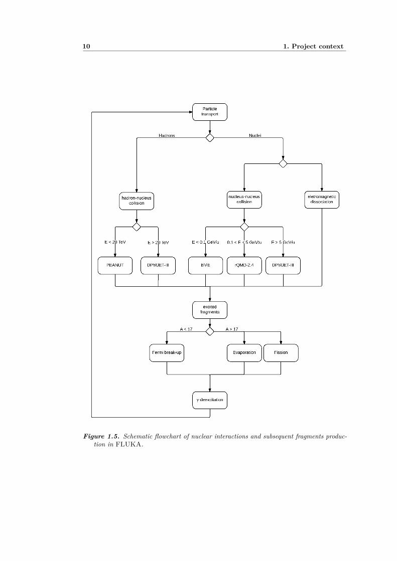
All the models described can produce excited fragments. If the mass numberof the fragment is smaller than 17, the deexcitation is described using an extendedFermi break-up model. If it is higher, the fragment can go in evaporation or fission,depending on the cross section, which in turn is function of the excitation energy.After this first step of deexcitation, all fragments can emit γ rays. A schematic flowchart of the nuclear interactions in FLUKA is depicted in Figure 1.5.
Hereinafter, the focus will be put on the lower energy nuclear interaction models,relevant for hadrontherapy (up to 100 MeV u−1) and for the simulations made for thiswork (33 MeV u−1). At such low energies, pion production is energetically impossiblein both nucleon-nucleon and nucleon-nuclei interactions. Hence nuclear interactionsat those energies consist of elastic nucleon-nucleon scatterings, that can result innucleon and light fragment emissions and can leave the remaining nuclei in an excitedstate.
1.6 Hadron-Nucleus interaction
In PEANUT the reaction mechanism is modelled by assuming a series of independentnucleon-nucleon collisions, i.e. an intra-nuclear cascade, smoothly joined to staticalpre-equilibrium emission if the energies of the nucleons are smaller than 50 MeV.However, to ensure continuity, in the region between 50 MeV and 10 MeV the nucleonsare still transported and, even though the interactions are not explicitly performed,the exciton number is increased and the pre-equilibrium stage will further developthe configuration. The statistical approach is used in the low-energy region, as thephysical foundation of the intra-nuclear cascade approach becomes invalid and canbe very time consuming as well.
In the intra-nuclear cascade, energy and momentum are conserved taking intoaccount the recoil of the residual nucleus. All the particles are transported consideringthe Coulomb and nuclear potentials. Path length and interaction mechanisms arechosen depending on the particle nucleon cross section and local density. The latteris evaluated as a function of the radius.
10 1. Project context
Figure 1.5. Schematic flowchart of nuclear interactions and subsequent fragments produc-tion in FLUKA.

1.6 Hadron-Nucleus interaction 11
A rejection method is applied to check, after each interaction, that the momentaof all secondary nucleons are above the Fermi level, to take into account Pauli’sexclusion principle. This increases the mean free path in a nuclear medium. Othershave the same influence. Among them, we can cite:
• nucleon anti-symmetrisation [BM69], which decreases the probability for sec-ondary particles to re-interact with a nucleon of the same type very close tothe production point
• nucleon-nucleon hard-core correlations [eal71], which also prevent secondaryparticles to collide again too close to the production point. Typical hard-coreradii used are in the range 0.5÷ 1 fm
• “coherence” length after elastic or charge exchange hadron-nucleon scatter-ings, because such interactions cannot be localised better than the positionuncertainty connected with the four-momentum transfer of the collision.
Nucleon-nucleon total cross sections, both elastic and inelastic, are taken fromavailable experimental data.
The pre-equilibrium statistical approach used in PEANUT is the exciton formal-ism, based on the so called Geometry Dependent Hybrid Model (GDH) [Bla71; Bla72;BV83; Bla83]. It consists in a recursive process where at each step a nucleon-nucleoncollision can increase the number of excitons by two. An exciton can be eithera particle above the Fermi level or a hole below it. At each step the probabilityof emitting a nucleon in the continuum is calculated. Indeed, at each step of thenucleon-nucleon interactions chain there is a probability P (ε) of emitting a nucleonin the continuum with energy ε. This probability can be factored in two parts: thefirst term gives the probability to have a particle with energy ε; the second oneexpress the probability of the exciton cluster to escape from the nucleus.
P (ε) = ρ(U, ε)gdερ(E)
rc(ε)rc(ε) + r+(ε) (1.9)
where g is the exciton state density; U is the residual nucleus excitation energy, i.e.U = E − ε−B; and ρ(E) is the density of exciton states, and is given by:
ρ(E) = g · (gE)n−1
n!(n− 1)! (1.10)
rc(ε) is the rate of emission in the continuum and r+(ε) is the exciton re-interactionrate, and can be calculated from the nucleon mean free path in nuclear matter.
r+ = fPauli(ε, EF ) [ρproσxp + ρneuσxn][2(ε+ V )
M
]1/2(1.11)
where V = EF +B and fPauli is the Pauli’s blocking suppression factor; M is theα mass; ρpro and ρneu are the densities respectively of protons and neutrons in thenucleus, σxp and σxn their cross section with the particle of kind x.
This model grounds on the assumption that all the possible partitions of theexcitation energy E among n excitons are equiprobable. The recursive process stops,

12 1. Project context
and equilibrium is reached, when either the exciton number n is sufficiently high(n =
√2gE , where g is the single particle level density) or the excitation energy
is below any emission threshold. The initial number of excitons depends on thereaction type and on the cascade history.
1.7 Low energy ion interaction
In the BME framework, the reaction cross section (σr) between two ions is calculatedusing a model developed [CCG05] on the basis of the “soft-spheres” model proposedby P. J. Karol [Kar75]. Two different main reaction paths have been adopted tosimulate the interactions: complete fusion, and peripheral collision. The choicebetween the two is made according to the partial cross section for complete fusion.From there, the probability of complete fusion is given by:
Pc.f. = σc.f.σr
(1.12)
and the one of peripheral collision is:
P = 1− Pc.f. (1.13)
In case of complete fusion, the new nucleus is the aggregate of the target andprojectile nuclei and is in an excited state. The de-excitation is simulated usingthe BME model, described in subsection 1.7.1. If the collision is peripheral, themodel predicts the formation of two or three fragments and extracts an impactparameter according to a distribution that takes into account the dependence of thenuclear density on the radius. The three bodies are the projectile-like fragment, thetarget-like fragment and a middle system, also called “fireball”. The latter fragmentis preferentially excited and its mass number is obtained integrating the projectileand target nuclei density distribution, which is assumed shaped as a Woods Saxonfunction, up to radii of the two nuclei that include 99% of the mass of the nuclei.The emission angle of the target and projectile-like fragment (θ) respects to thedirection of flight of the projectile in the center of mass frame is sampled from anexponential decreasing distribution exp(−kθ) whose parameter k is a function of thefragments masses and of their energies. Their momentum moduli are sampled froma phenomenological energy loss distribution. The emission angle and the momentummodulus of the fireball are defined by the momentum conservation. The excitationenergy, subtracted from the kinetic energy as energy lost, is shared between thethree fragments preferring the fireball. The excitation energy of the fireball is aquadratic function of the mass of the fireball itself.
The fireball de-excitation is simulated using the BME model, if the two fragmentsthat composed it fit in the pre-computed database, or PEANUT [FSFR05].
1.7.1 Boltzmann Master Equations
Nucleus-nucleus interactions produce excited nuclei that can be the residual partof the projectile, of the target nucleus or of a composition, even partial, of thetwo. As said before, to describe the thermalisation of the latter, when produced

1.7 Low energy ion interaction 13
in a certain region of the projectile and target parameters space, the BoltzmannMaster Equation (BME) theory [CFGER98] is used. This theory estimates the timevariation of nucleons momenta distribution as a result of their mutual interactions.The theory predict also the nucleons emission into the continuum, as separate entitiesor as part of a cluster. For this aim, the phase space is divided in bins of volume∆V = 2πm∆ε∆pz, where m is the nucleon mass, ε its energy and pz its momentumprojection along the beam axis. The time evolution of the occupation probabilityni(ε, θ, t) of the bin i is calculated using a set of coupled differential equations:
d(nigi)P
dt=∑j,l,m
[ωPPlm→ijg
Pl n
Pl g
Pmn
Pm
(1− nPi
) (1− nPj
)+
− ωPPij→lmgPi nPi gPj nPj(1− nPl
) (1− nPm
)]+
+∑j,l,m
[ωPNlm→ijg
Pl n
Pl g
Nmn
Nm
(1− nPi
) (1− nNj
)+
−ωPNij→lmgPi nPi gNj nNj(1− nPl
) (1− nNm
)]+
−nPi gPi ωPi→i′gPi′ δ(εPi − εPF −BP − εPi′
)− dDP
i
dt
(1.14)
where P and N indicate respectively Protons and neutrons; gi is the total numberof states in the ith bin; the terms such as ωij→lm are the transition probability perunit time that, in a two-nucleon interaction, nucleons in bins i and j go to bins l andm; ωPi→i′ is the single Proton emission probability from the bin i to the continuumand finally dDP
i /dt is the depletion term which accounts for the Proton emissionfrom the bin i as part of a cluster. A set of equation analogous to Equation 1.14holds for the neutron states as well.
A cluster is defined as the coalescence of nucleons with momenta closer eachother than a given value (pc,F ). If it is not emitted immediately, it is not consideredas a cluster in the subsequent time step. The cluster formation probability wc attime t in the portion of the phase space Ec, θc with Zc Protons and Nc neutrons is:
wc(Ec, θc, t) =∏i
(nPi (ε, θ, t)
)Pi(Ec,θc)Zc
·∏i
(nNi (ε, θ, t)
)Pi(Ec,θc)Nc
(1.15)
where Pi(Ec, θc) is the volume fraction of the bin i within a sphere of radius pc,Fcentred in Ec, θc in the phase space. The probability of emitting a neutron, withenergy Ec in one of the bin of the momentum space can be obtained as a specialcase of the Equation 1.15 setting Nc as one and Zc as zero, Pi(Ec, θc) is zero for allthe combination Ec and θc except for the chosen one where it is one.
From the probability of formation of a cluster (Equation 1.15) it is possible tocalculate the multiplicity spectrum of this cluster:
d2Mc(E′c, θc)dE′cdΩc
= Rc2πsin(θc)
∫Nc(Ec, θc, t)
σinvvcV
ρc(E′c, θc)dt (1.16)
where E′c is the cluster energy once emitted outside of the nucleus; σinv is the crosssection for the inverse process, that is the cluster absorption from the residualnucleus; V is the volume of the continuum and cancels with an equal term appearing

14 1. Project context
in ρc(E′c, θc), the density of cluster states in the continuum; Rc is the probabilitythat the cluster is emitted after being formed
By integrating the Equation 1.14, it is possible to obtain the time evolution ofthe nucleons in the phase space, i.e. the thermalisation of the nucleus. The integralof the differential multiplicity (Equation 1.16) is the total number of fragments cproduced.
Anyway, this approach cannot be implemented in a transport code such asFLUKA because the run-time calculation of the multiplicity spectra for all thepossible ejectiles is too long. Thus the implementation of the BME in FLUKAhas been done by precomputing off-line and then fitting the predicted ejectilesmultiplicity and double-differential spectra with analytical expressions described bya small set of parameters [CBC06].
1.7.2 Fermi Break-up
The cascade and pre-equilibrium stages can produce excited nuclei. These nuclei aresupposed to be in an equilibrated state, i.e. the excitation energy U is statisticallyshared among all possible configurations. Each nucleus is characterised by its mass,charge and excitation energy. Since the excitation energy can be higher than theseparation energy, the emission of nucleons and light fragments is still possible.
As seen in the flow chart 1.5, for light nuclei (with A ≤ 17) the so-called FermiBreak-up model [Fer50; ÉG67] is used to describe the emission of one or morefragments from the excited nucleus. The emission is simulated in only one step.The branching ratios between the possible ejectiles are calculated from phase spaceconsiderations. More specifically, the probability W for disassembling a nucleus ofN neutrons, Z Protons, with an excitation energy U into n fragments (n ≥ 2) isgiven by:
W = SnG
[Vbr
(2π~)3
]n−1(
1M∗
n∏i=1
mi
)3/2 (2π)3(n−1)/2
Γ(32(n− 1))
E3n−5
2kin (1.17)
where Ekin is the total kinetic energy of all the fragments at the moment of break-up,M∗ is the total mass (M∗ = U +MA +MZ), mi the mass of the i fragment and Vbris a volume of the order of the initial residual nucleus volume. The spin Sn and thepermutation G factors are given by:
Sn =n∏i=1
(2Si + 1), G =k∏j=1
nj ! (1.18)
in which nj is the number of identical particles of the jth kind.Therefore, evaluating the probability 1.17 for all energetically allowed combina-
tions of fragments, it is possible to extract the final state. In the FLUKA extensionof the Fermi break-up formalism, constraints on available configurations and thecentrifugal barrier (if L = 0 is forbidden) are taken into account in cases where thespin and parity of the excited nucleus are known [BCC+14].
In FLUKA, all stable particles with A ≤ 16 and a few unstable isotopes, like8Be, are possible ejectiles. If the produced nucleus is unstable, it is left to decay

1.7 Low energy ion interaction 15
according to the experimental branching. Once the final state configuration has beenselected, the kinematical quantities of each fragment are chosen according to n-bodyphase space distribution. Such a selection is performed taking into account theCoulomb repulsion between all charged particles. In practice, Ekin at disassemblingis given by:
Ekin = U −(
n∑i=1
mic2 −MA,Zc
2)−BCoul (1.19)
where also the emitted fragments can be in an excited state. The total Coulombbarrier BCoul of the selected configuration is distributed to charged particles afterdisassembling, in their own center of mass system.


17
Chapter 2
Experiment
2.1 Experimental Facility
The experiment was realised at iThemba Laboratories, a multidisciplinary facilitylocated near Somerset West in Cape Town, South Africa. This laboratory providesaccelerator and ancillary facilities that are used for research and training in nuclearand accelerator physics, radiation biophysics, radiochemical and material sciences,radio nuclide production and radiotherapy. Patients are treated during the day,and between treatments the beam is switched to the radio nuclide production vault.Over the weekend, beams of light, heavy ions and polarised protons are used fornuclear physics experiments.
The cyclotron in use can accelerate proton beams up to 200 MeV. It can alsoaccelerate heavier ions to energies up to 33.3 MeV u−1 depending on the beam species.In this experiment, a 12C beam of 33.3 MeV u−1 has been used.
2.2 Experimental Setup
This experiment was carried out in the A-line scattering chamber, which consistsof a vacuum chamber of about 1.5 m in diameter and has a target ladder in thecentre and two rotating arms to host the detectors. The ladder is in aluminiumand can host up to five different targets arranged vertically. Both the detector armsand the target ladder can be moved remotely in order to change the setup withouthaving to break the vacuum every time. During the data taking, the pressure in thescattering chamber has been kept around 10−5mbar. The vacuum was made usingin sequence a rotary pump to reach a pressure of 1 mbar, a turbomolecular pumpup to 10−3mbar, and finally a cryogenic pump.
Four different kinds of target have been used for the experiment under consider-ation: Carbon (C), Gold (Au), Niobium (Nb) and lastly, to explore the possibilityof Hydrogen contamination on the targets surfaces, Polyethylene
((CH2)n
). The
thickness and the density of the targets are reported in table 2.1.The set of detectors placed on the right arm is referred to as the “α telescope”,
while the set on the other arm as the “Be telescope”. A schematic diagram of theexperimental setup is shown in figure 2.1.

18 2. Experiment
Table 2.1. Thickness and density of the targets used in the experiment.
Target material Density [g cm−3] Thickness [µm]C 2.0 5.265Nb 1.05 0.466Au 19.32 1.22
(CH2)n 0.96 6 1
The α telescope is constituted by a collimator, two silicon detectors and a sodium-iodide scintillator (NaI). The collimator is in brass and its thickness is 3 cm with a1.4 cm diameter opening. As the distance between the target and the back of thecollimator is 29.1 cm, the solid angle subtended by the acceptance of this telescope is1.82 msr. The thickness of the first (∆E1) and of the second (∆E2) silicon detectoris respectively 21 µm and 541 µm.
The 8Be telescope consists of a Silicon Strip Detector (SSD) followed by a NaI,alike to the one in the α telescope. The SSD is made of 16 vertical strips. Each strip
Figure 2.1. Schematic diagram of the A-line scattering chamber showing the two rotatingarms hosting the 8Be telescope, composed by the SSD and a Sodium-iodide scintillator,and the α telescope, which consists of two silicon detectors and another Sodium-iodidescintillator. The distances between the target and the detectors are uninformative.
is 3 mm wide with an inter-strip separation of 0.1 mm. The total active surface ofthe SSD is a square with a side of 5.0 cm and 251 µm thick. Between the SSD andthe subsequent NaI there is a brass circular collimator with an inner diameter of6.0 cm and the back side 56.89 cm far from the target (3.43 msr).
1This value is uncertain.

2.2 Experimental Setup 19
The two NaI’s are identical: they are cylindrical with a diameter of 7.6 cm andthickness of 5.1 cm and both are coupled to a photomultiplier. A light pulser hasbeen used to correct the instabilities in each of the photomultipliers. The NaI’s havebeen protected from the atmospheric moisture in the scattering chamber before thevacuum with a 7 µm thick foil of Havar.
Two triggers have been defined, one for each telescope. The trigger relative tothe 8Be telescope fires when the SSD and the NaI measure an energy deposition;the α one fires when the ∆E1 and the ∆E2 or the ∆E2 and the NaI go over thethresholds. The coincidence trigger fires when both the single telescope triggersfire. All the coincidence triggers and 5% of the single trigger events are acquired,the latter in order to be compared with the data already published in [GSB+01].More details about the experiment setup can be found in [Mir11]. To measure alsothe angular dependence of the quasi-elastic 12C break-up, different runs have beenperformed with the α telescope placed at 16, 18, 20, 22 and 24 from the beamaxis, while the 8Be telescope is always placed at 9.
2.2.1 Calibration
The energy calibration of the ∆E2 and the SSD has been performed in vacuumplacing a 208Th source in the scattering chamber. A typical spectrum can beseen in figure 2.2. As the highest energy α emitted from the 208Th has 8.78 MeV,CHAPTER 3. DATA ANALYSIS 33
Figure 3.1: Typical energy spectrum of the α particles from a 228Th sourcemeasured with the Si ∆E2, T1B, T1C and T2A detectors showing the energies ofemitted α-particles in MeV.
source for other Si detectors as previously described. The high energy calibra-tion was performed with the elastic scattered 12C beam on a thin 197Au target.In order to get calibration points the detector telescope was placed at differentemission angle ranging from 8 to 15. The elastic peak of scattered 12C wereidentified together with their corresponding channel numbers. The elastic peakenergies were plotted against their corresponding channel numbers. The slopeand offset parameters of the energy calibrations were determined by linear fitjoining both the lower energy and higher energy calibration points. Fig. ??shows the typical α-particle energy spectrum, and Figs. ?? to ?? show thecalibration curves for different silicon detectors as indicated on the caption.
3.4.2 Silicon ∆E1 and T1A detectors
This section explain about the energy calibration of both the 21 µm thick ∆E1
used for the correlations experiment on the α-particle detector arm as well asthe 57 µm thick T1A Silicon detector used on the heavier fragments arm forIMFs measurement. The calibration was performed by using the calibrationparameters of the transmission detectors on both occasions which are ∆E2
and T1B Silicon Detectors, respectively. This was done due to the fact that
Figure 2.2. Typical spectrum of 208Th measured with the ∆E2. Plot from [Mir11].
the calibration points obtained from the 208Th have been complemented with themeasurement of the elastic peak of the 12C scattered from a thin gold target. Theelastic peak has been measured placing the detectors at different angles from 8 to15. The slope and the offset used to convert the acquired values in energy havebeen obtained with a linear fit of the two data sets.
Since the ∆E1 silicon detector is not thick enough to stop the α particle emittedby the 208Th, it has originally been calibrated fitting the measured energy loss of

20 2. Experiment
α particle stopped in the ∆E2 detector with the value predicted by the ELOSSprogram [Jip84]. This calibration is constrained to go through the origin and the fithas been used to calculate the value of the angular coefficient. During the analysis,a small discrepancy has been found between the data and the MC in the responseof the ∆E1 detector. It has been hypothesised that this discrepancy is ascribableto the calibration. For this reason, the calibration has been modified. The energydeposited in the ∆E1 by α particles in the energy range 0 ÷ 35 MeV, i.e. the α’sstopped by the ∆E2, has been recalculated making a dedicated simulation withFLUKA. These values are shown in Figure 2.3. The correction to the calibration
E2 [MeV]∆0 5 10 15 20 25 30 35 40
E1
[MeV
]∆
0
0.5
1
1.5
2
2.5
3
3.5
4
4.5
Figure 2.3. Energy deposited in ∆E1 as a function of the energy deposited in ∆E2 by αparticles calculated with a FLUKA simulation.
has been done minimising the function:
χ2(m, q) =Nbin∑i=1
[(m · 〈Expi〉+ q)−MCi
]2σ2Expi
+ σ2MCi
(2.1)
where 〈Expi〉 is the average of the energy deposited in the ∆E1 for each bin of theenergy deposited by the α’s in the ∆E2 detector. The α’s are selected in a similarway as described in 4.4, but the energy deposited in the NaI placed after the twosilicon detectors of the α telescope must be zero in order to select only the α thatstops in the ∆E2. MCi are the calculated energy deposition in ∆E1 with the MCsimulation. σ2
Expiand σ2
MCi are respectively the variance of 〈Expi〉 and MCi. mand q are the parameters of the calibration, m is a multiplicative factor to correctthe calibration previously done, and q the offset left as a free parameter for theminimisation. The result of the minimisation, made with MINUIT2 [JR75], is shownin Table 2.2
The original calibration was made imposing the intercept to be zero. Conversely,letting the intercept as a free parameter, its best value is not compatible with zero

2.2 Experimental Setup 21
Table 2.2. Correction parameters to the calibration of the ∆E1 calibration.
Value σ
m 0.9 0.1q [MeV] 0.10 0.02
and is of the order of magnitude of the offset subtracted during the data taking. Thebest value for the angular coefficient is 10% smaller. The effect of this correction isshown in Figure 2.4 and is more evident in the region of high ∆E1.
E2 [MeV]∆0 5 10 15 20 25 30 35 40
E1
[MeV
]∆
0
1
2
3
4
5
6
7
-110
1
10
(a)
E2 [MeV]∆0 5 10 15 20 25 30 35 40
E1
[MeV
]∆
0
1
2
3
4
5
6
7
-110
1
10
210
(b)
Figure 2.4. Energy measured by the ∆E1 detector as a function of the energy measuredby the ∆E2 detector. The blue points are the value calculated with a MC simulationand seen in Figure 2.3. The left panel shows the data with the original ∆E1 calibrationwhile the right one shows the data with the new calibration, with the intercept as a freeparameter. The difference between the two calibrations is more evident in the region ofhigh ∆E1.
The two NaI’s have been calibrated using only the 12C elastic peak response asnormalization parameter for the light output predicted by the model of Michaelianet al. [MMRBM93], more details about the calibration of the two NaI’s can be foundin [SFL+05].
2.2.2 Data preparation
The data were originally stored in a binary format for VAX servers. To performthe analysis using ROOT [BR97] the data have been converted in ROOT files. Theconversion has been done in two steps: firstly a Fortran program has been developedto export the binary file from the VAX server into a CSV file, secondly these fileshave been converted in TTree ROOT files using a C++ program. For each run, adifferent file has been created to keep the size of each file small and easy to handle.Each file contains also the information about the pulser of the two NaI’s and thecalibration parameters of all the detectors.

23
Chapter 3
Monte Carlo simulation
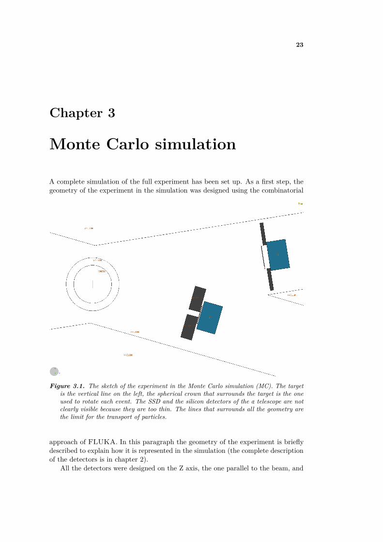
A complete simulation of the full experiment has been set up. As a first step, thegeometry of the experiment in the simulation was designed using the combinatorial
Figure 3.1. The sketch of the experiment in the Monte Carlo simulation (MC). The targetis the vertical line on the left, the spherical crown that surrounds the target is the oneused to rotate each event. The SSD and the silicon detectors of the α telescope are notclearly visible because they are too thin. The lines that surrounds all the geometry arethe limit for the transport of particles.
approach of FLUKA. In this paragraph the geometry of the experiment is brieflydescribed to explain how it is represented in the simulation (the complete descriptionof the detectors is in chapter 2).
All the detectors were designed on the Z axis, the one parallel to the beam, and

24 3. Monte Carlo simulation
then rotated by the proper angle, thus allowing to modify easily the angle of the αtelescope for the different runs.
In the experiment there are two collimators. One is placed in front of the firstsilicon detector (∆E1) in the α telescope and the second one is placed betweenthe SSD and the NaI in the 8Be telescope; both are made of brass while in thesimulation they are made of a special material called “blackhole”. In FLUKA anyparticle that enters a region made of this material is not transported anymore. Thisapproximation is validated by a dedicated simulation (plots 3.2 and 3.3) with thecollimators in brass. This simulation showes that the current of charged particlesout coming from the collimators is two order of magnitudes less than the current ofcharged particles passing through the collimators. Therefore, the secondary particlesproduction in the two collimators can be neglected.
Figure 3.2. Currents of charged particles (green) and α (red) passing through the 8Betelescope collimator and current of charged particles produced in the collimator (blue).
The description of the α telescope is quite simple: two cylindric silicon detectorswhich have a sensitive area larger than the collimator in front of them and acylindrical NaI scintillator at the end.
The 8Be telescope is more complex: the first element is the SSD. This detectoris made of one silicon layer divided in 16 strips. As in MC each strip is a separateregion, the energy deposition can be scored in each of them separately. After the SSDthere is one of the collimators, followed by a NaI scintillator. The area subtendedby this collimator is smaller than the SSD active surface. Indeed, as the active areaof the SSD has the shape of a square with a side of 5 cm while the collimator iscircular with a diameter of 6 cm, it is necessary to insert in the simulation also theframe of the SSD. The SSD frame is made of epoxy resin with an increased density(1.85 g cm−2) because moulded epoxy has fillers of glass fiber. A layer of 50 µm incopper has been added to simulate the printed circuit board. Also the Havar windowin front of the two NaI detectors has been inserted in the simulation. A sketch of

3.1 Implementation of the simulation 25
Figure 3.3. Currents of charged particles (green) and α (red) passing through the α telescopecollimator and current of charged particles produced in the collimator (blue).
the modelled geometry is shown in figure 3.1.Since the targets used in the experiment are all very thin, (see table 2.1 in
Chapter 2) the MC starts directly with the simulation of the interaction betweenthe projectile and the target nuclei without transporting a primary bream particlethrough the target. Afterwords, the output is weighted by the cross section of theprocess. To investigate the hypothesis of a H contamination in the targets andsimulate the Polyethylene one, the MC has been run twice, once to simulate the Hand once for the other element.
3.1 Implementation of the simulation
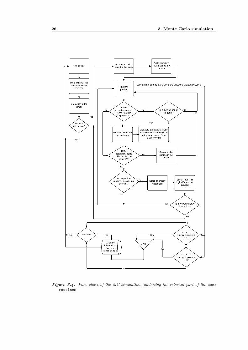
For analysis purpose, the data are scored event by event, making extensive use ofuser routines developed for this analysis. A common, to save the information foreach event, has been defined. A flow chart of the code is presented in figure 3.4.
When a new secondary particle is placed in the stack, its data and data aboutthe particle and the interaction that generated it are saved. Furthermore a variablethat counts the number of secondaries in the event is incremented. This progressivenumber is used also as a flag to identify the particle in each of the subsequent steps.
For each detector an array has been defined. Each element in the array is usedto score the energy deposition of one particle. The strips of the SSD are treated asseparate detectors, indeed the energy deposition is saved separately for each of them.For the two NaI scintillators, the energy deposition and the light output simulatingthe quenching are saved. Details about the simulation of the quenching will be givenin section 3.3. The energy deposition are saved also for some of the passive elementsof the geometry, such as the Havar windows placed in front of the scintillators andthe SSD frame.
26 3. Monte Carlo simulation
Figure 3.4. Flow chart of the MC simulation, underling the relevant part of the userroutines.
3.2 Biasing 27
As in the experiment, a single trigger for each telescope has been defined. Inthe 8Be telescope, the trigger is the coincidence between one strip of the SSD andthe NaI that is placed after it; in the α telescope, it is the coincidence of two of thethree detectors. All the coincidences between the two telescopes triggers and 5% ofthe single trigger events are stored. To simulate the experimental output, also theinformation about the trigger that fired is saved.
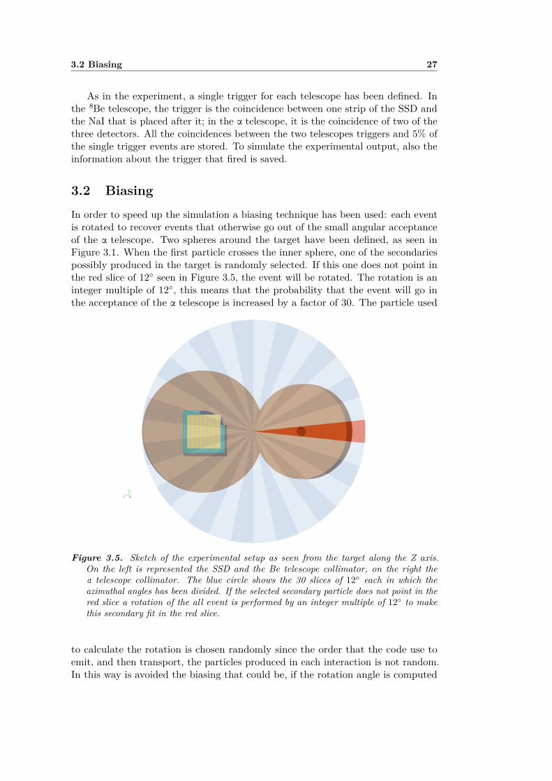
3.2 Biasing
In order to speed up the simulation a biasing technique has been used: each eventis rotated to recover events that otherwise go out of the small angular acceptanceof the α telescope. Two spheres around the target have been defined, as seen inFigure 3.1. When the first particle crosses the inner sphere, one of the secondariespossibly produced in the target is randomly selected. If this one does not point inthe red slice of 12 seen in Figure 3.5, the event will be rotated. The rotation is aninteger multiple of 12, this means that the probability that the event will go inthe acceptance of the α telescope is increased by a factor of 30. The particle used
Figure 3.5. Sketch of the experimental setup as seen from the target along the Z axis.On the left is represented the SSD and the Be telescope collimator, on the right theα telescope collimator. The blue circle shows the 30 slices of 12 each in which theazimuthal angles has been divided. If the selected secondary particle does not point in thered slice a rotation of the all event is performed by an integer multiple of 12 to makethis secondary fit in the red slice.
to calculate the rotation is chosen randomly since the order that the code use toemit, and then transport, the particles produced in each interaction is not random.In this way is avoided the biasing that could be, if the rotation angle is computed
28 3. Monte Carlo simulation
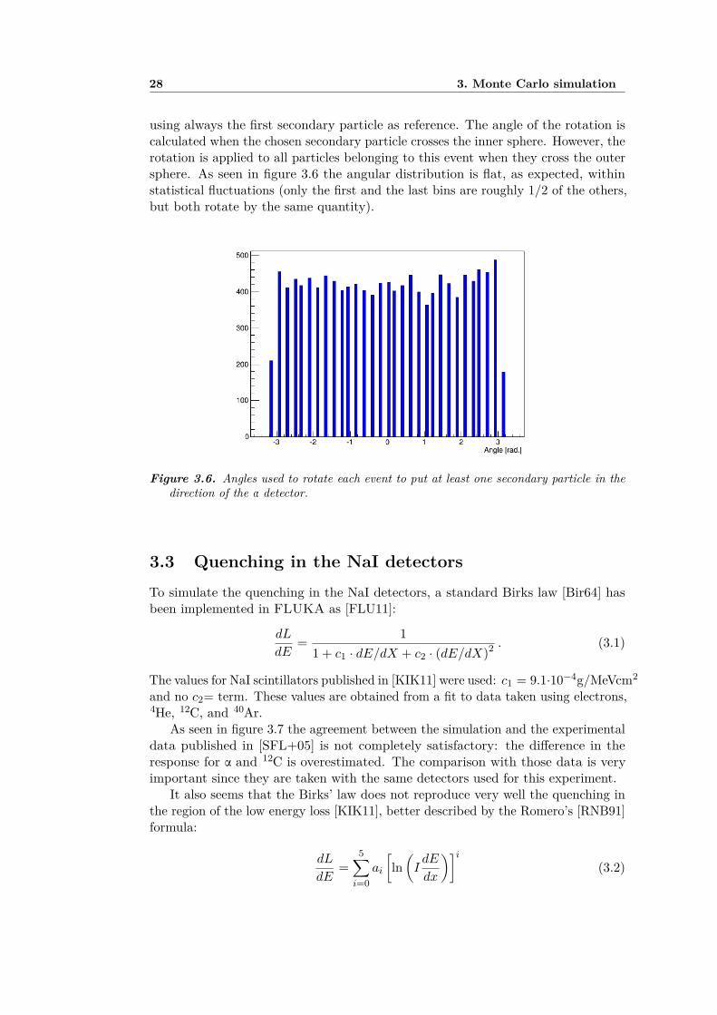
using always the first secondary particle as reference. The angle of the rotation iscalculated when the chosen secondary particle crosses the inner sphere. However, therotation is applied to all particles belonging to this event when they cross the outersphere. As seen in figure 3.6 the angular distribution is flat, as expected, withinstatistical fluctuations (only the first and the last bins are roughly 1/2 of the others,but both rotate by the same quantity).
Figure 3.6. Angles used to rotate each event to put at least one secondary particle in thedirection of the α detector.
3.3 Quenching in the NaI detectorsTo simulate the quenching in the NaI detectors, a standard Birks law [Bir64] hasbeen implemented in FLUKA as [FLU11]:
dL
dE= 1
1 + c1 · dE/dX + c2 · (dE/dX)2 . (3.1)
The values for NaI scintillators published in [KIK11] were used: c1 = 9.1·10−4g/MeVcm2
and no c2= term. These values are obtained from a fit to data taken using electrons,4He, 12C, and 40Ar.
As seen in figure 3.7 the agreement between the simulation and the experimentaldata published in [SFL+05] is not completely satisfactory: the difference in theresponse for α and 12C is overestimated. The comparison with those data is veryimportant since they are taken with the same detectors used for this experiment.
It also seems that the Birks’ law does not reproduce very well the quenching inthe region of the low energy loss [KIK11], better described by the Romero’s [RNB91]formula:
dL
dE=
5∑i=0
ai
[ln(IdE
dx
)]i(3.2)

3.3 Quenching in the NaI detectors 29
Figure 3.7. Light output of the NaI, the black histogram is the simulation for 12C andα using the Birks’ law (eq. 3.1). The red and blue dots are experimental points from[SFL+05] for He and C respectively.
where I is a constant that has the value of 1 g cm2 MeV−1. The coefficients ai area-dimensional and obtained with a fit from experimental data. The set of valuesthat let the equation 3.2 better fit the data are reported in the table 3.1 and areobtained with experiments made using beams of electrons, protons, deuterons, α,20Ne and Na [RNB91].
Table 3.1. Coefficients used in the equation 3.2. From [RNB91]
a0 0.68a1 0.12a2 0.045a3 -0.022a4 2.3 · 10−3
a5 −7.3 · 10−5
As seen in figure 3.8 this implementation describes better the differences in lightoutput of a NaI detector between α and 12C. There is a small discrepancy, but itis in the high energy region of the 12C ions and it should not affect the simulation.In fact, high energy 12C ions will not reach the detector in the MC simulation andwould not match the selection criteria anyway.

30 3. Monte Carlo simulation
Figure 3.8. Same as Figure 3.7 but the simulation is made using the Romero’s descriptionof the Birks law (eq. 3.2).
3.4 Data preparation
When one of the possible triggers fires, the event is written on disk. For each eventseveral lines are written, each of them starts with a string that identifies the lineitself. The first line of each event contains information about the event in general,such as the number of the primary (it is a sequential counter for the primariessimulated), the number of secondaries in the event, the trigger that fired, the numberof secondaries produced in the target and the flag of the secondary particle extractedto calculate the angle used to rotate the event.
Afterwards, for each secondary the program writes:
• the particle ID;
• the sequential flag assigned to recognise them;
• a flag to distinguish the interaction that produced this secondary;
• the particle id of the particle that generated it;
• the sequential flag of the particle that generated it;
• the number of the generation, i.e. 0 for the primary, 1 for the particle generatedfrom the primary and so on;
• the energy deposition in each detector and relevant passive element, exceptthe SSD;
• the statistical weight;
• the light output of the two NaI scintillators.

3.4 Data preparation 31
The strips of the SSD, but only those where there is an energy deposition, arewritten one by one. In other words, for each secondary there is a line if the secondarydeposited some energy in one strip. The information saved includes the strip number,the particle flag (to check that there was no error in the identification) and theenergy deposition.
After the data about the secondaries, information about the last Fermi breakup-such as the number of fragments produced, their atomic and mass number and theirexcitation energy- are stored.
As for the experimental data, a program in C++ to convert the output ofFLUKA in ROOT data files has been developed.
Inside this program the variables and branch names for all the quantities thatexist also in the experimental data have the same name, in order to allow the use ofthe same code for the analysis of the MC and experimental data.
For each simulation run, a ROOT file has been created in order to have filesof small size. During the analysis all the data, relative to the same experimentalconditions, are collected from the different files in a TChain.
To speed up the running of the code for each simulation, 50 different simulationsare executed in parallel with different random seeds.


33
Chapter 4
Data Analysis
This chapter presents the description of the experimental data analysis starting fromthe MC simulation described in chapter 3. The FLUKA framework has been usedto simulate the response of the detectors and the kinematic of the 8Be decay toaddress the selection criteria.
4.1 Scintillator resolutionIn order to reproduce the resolution of the two NaI’s, a convolution with a Gaussiandistribution centred in 0 has been applied to the simulated light output in theanalysis code. Since the two NaI’s have different resolutions they have been evaluatedseparately using their response to the elastic scattered beam particles.
The selection of the beam particles in the Be telescope has been performed takingonly the single triggers of the 8Be telescope, and using only one strip of the SSD, toreduce the angular acceptance. The C scattered ion are selected requiring an energydeposition in the chosen strip greater than 19 MeV. The events selected in this wayare shown in Figure 4.1.
For the NaI in the α telescope it has been requested that the energy depositionin the ∆E1 is in the range 2÷ 3 MeV because the energy loss the C ion with thisenergy is 2.4 MeV. The event selected for the α telescope are shown in Figure 4.2.They are much less than in the Figure 4.1 because the Be telescope is at 9 respectto the beam axis, while the α one is at least at 16, the configuration used forthis evaluation. Moreover the angular acceptance of the α telescope is one order ofmagnitude smaller than the acceptance of the Be telescope.
In these plots the energy scale is arbitrary because the calibration has been donefor the α particles and, as seen in section 3.3, the response of the scintillators isdifferent for the different particle species. Since the counting statistic allows to usethe Poisson distribution, the resolution of the NaI’s scales as the square root of themeasured energy (E). Therefore, the standard deviation of the smearing functioncan be expressed as:
σsmearing = σC
√E
õC
. (4.1)
Where σC and µC are respectively the standard deviation and the mean of theGaussian at the elastic peak of C ions beam. This is an approximation, because it

34 4. Data Analysis
E [a.u.]140 160 180 200 220 240 260 280
Cou
nts
[a.u
.]
0
200
400
600
800
1000
1200
1400
Figure 4.1. Energy deposition in the NaI by the elastic scattered beam particles, in blue.The energy on the x axis is calibrated for the response of the NaI to α particles. In redthe gaussian fit made to estimate the resolution of the detector.
E [a.u]180 190 200 210 220 230 240
Cou
nts
[a.u
.]
0
2
4
6
8
10
12
14
16
18
Figure 4.2. Same as Figure 4.1 but for the NaI in the α telescope.

4.2 Particle Identification 35
does not take into account non linearities, but with only one experimental point perdetector it is the best estimation we could do. To measure the parameters in theEquation 4.1, two fits have been done and the result are shown in Table 4.1.
Table 4.1. Fit parameters of the two NaI’s resolution.
telescope µC σC[MeV] [MeV]
α 216.5± 0.8 1.3± 0.8Be 222.5± 0.1 3.8± 0.1
The different resolution of the two NaI’s is not surprising. In fact, the twocrystals are identical but the two photomultipliers are different. Because of thelimited space in the 8Be telescope, the photomultiplier in it is custom made: it isshorter and has a poorer photostatistics than the other one.
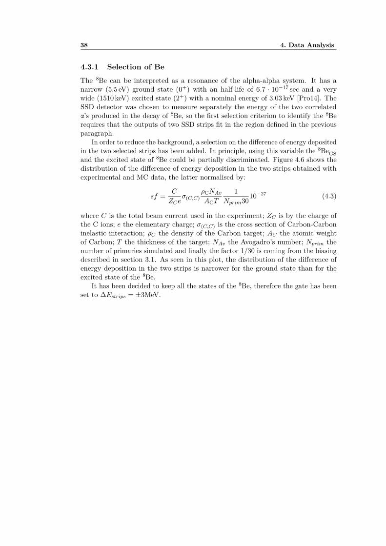
4.2 Particle IdentificationThe two correlated α’s in the 8Be telescope and the α in the other telescope wereidentified through the ∆E/E method. It consists in binning the energy depositionin a thin detector (a passing through detector) as a function of the particle energyin bi-dimensional histograms, where the latter is measured with another detectorthick enough to stop the particles. Hereinafter more details will be given describingseparately the two telescopes. All the data presented in this section, both the MCand the experimental ones, relate to the carbon target with the α telescope placed at16 because the selection criteria defined for the other targets and other orientationof the α telescope are the same.
4.3 Be telescopeAs described in chapter 2, the 8Be telescope is made of a thin silicon detector, theSSD, and a NaI. The signal is generated by two correlated α’s resulting from thedecay of 8Be. The two correlated α’s cross the SSD in two different strips and bothreach the NaI. Let ∆Eα(E) be the energy deposition of one α particle in the SSDas a function of the energy deposition (E) in the subsequent NaI. This functionhas been obtained using the FLUKA driver that simulates the energy loss. Sincethe binding energy of 8BeGS is just 92 keV, the phase space is small and the twoα’s coming from the 8BeGS decays have almost the same energy. In addition, thestrips are read out separately, hence the signal energy deposition ∆EBe(E) can beapproximated as:
∆EBe(E) ≈ ∆Eα(E
2
). (4.2)
Figure 4.3 shows the energy deposition in the SSD as a function of the one inthe NaI, as provided by the MC simulation of the experiment. Conversely, figure 4.4shows the energy deposition made only by the signal. In both figures the black line

36 4. Data Analysis
is the expected energy deposition of the signal ∆EBe(E). Considering their purpose,we will refer to these plots as PID plots.
NaI (Be) [MeV]50 100 150 200 250 300 350 400 450
SS
D [M
eV]
2
4
6
8
10
12
14
16
18
1
10
210
310
410
Figure 4.3. Energy deposition in the SSD as a function of NaI. Data from the MCsimulation. The black line is the expected energy deposition from two correlated α’s, whilethe blue one is the expected energy deposition of a single α. The red lines delimit theselected region (for the low energy part, the lowest between the magenta and the red ischosen, where the magenta is the expected energy deposition of a single α +1 MeV).
To isolate the signal in figure 4.3 a region has been defined to include all thesignal. The lower cut is set at
EDSSSD −∆EBe(E = ENaI) = −1.4 MeV ,
while the higher one at
EDSSSD −∆EBe(E = ENaI) = 2.0 MeV
The selected region is represented in the plots 4.3 and 4.4 by the two red lines. Toensure the selection of all the signal, a less strict criterion has been chosen for the lowenergy region: the expected energy deposition of a single α increased by 1 MeV. Thelower cut is then the smaller between ∆EBe(E)− 1.4 MeV and ∆Eα(E) + 1.0 MeV.The value of 1 MeV has been chosen since the curve ∆Eα(E) + 1.0 delimits theregion in figure 4.3 corresponding to the single α signal. It is represented by themagenta line in figures 4.3 and 4.4. The final selected region is shown in figure 4.5,on the top of the experimental data.
The histograms in the plots 4.3, 4.4 and 4.5 are filled with the data from allthe strips since, after the calibration, the response of all of them is the same. Theselection is applied on the data strip by strip and two strips matching the selectioncriteria are requested.

4.3 Be telescope 37
NaI (Be) [MeV]50 100 150 200 250 300 350 400 450
SS
D [M
eV]
2
4
6
8
10
12
14
16
18
1
10
210
310
410
Figure 4.4. As in figure 4.3, the plot shows the response of the SSD as a function of NaI,but here only the energy deposition due to the α’s from 8Be is taken into account. Thecolor code is the same of figure 4.3.
NaI (Be) [MeV]50 100 150 200 250 300 350 400 450
SS
D [M
eV]
2
4
6
8
10
12
14
16
18
1
10
210
310
410
Figure 4.5. This plot is the same of the figure 4.3 but obtained with experimental data. Theblack line is the expected energy deposition from two correlated α. The red line delimitsthe selected region.
38 4. Data Analysis
4.3.1 Selection of Be
The 8Be can be interpreted as a resonance of the alpha-alpha system. It has anarrow (5.5 eV) ground state (0+) with an half-life of 6.7 · 10−17 sec and a verywide (1510 keV) excited state (2+) with a nominal energy of 3.03 keV [Pro14]. TheSSD detector was chosen to measure separately the energy of the two correlatedα’s produced in the decay of 8Be, so the first selection criterion to identify the 8Berequires that the outputs of two SSD strips fit in the region defined in the previousparagraph.
In order to reduce the background, a selection on the difference of energy depositedin the two selected strips has been added. In principle, using this variable the 8BeGSand the excited state of 8Be could be partially discriminated. Figure 4.6 shows thedistribution of the difference of energy deposition in the two strips obtained withexperimental and MC data, the latter normalised by:
sf = C
ZCeσ(C,C)
ρCNAv
ACT
1Nprim3010−27 (4.3)
where C is the total beam current used in the experiment; ZC is by the charge ofthe C ions; e the elementary charge; σ(C,C) is the cross section of Carbon-Carboninelastic interaction; ρC the density of the Carbon target; AC the atomic weightof Carbon; T the thickness of the target; NAv the Avogadro’s number; Nprim thenumber of primaries simulated and finally the factor 1/30 is coming from the biasingdescribed in section 3.1. As seen in this plot, the distribution of the difference ofenergy deposition in the two strips is narrower for the ground state than for theexcited state of the 8Be.
It has been decided to keep all the states of the 8Be, therefore the gate has beenset to ∆Estrips = ±3MeV.

4.4 α telescope 39
strip1 - strip2 [MeV]-6 -4 -2 0 2 4 6
Co
un
ts [
a.u
.]
0
100
200
300
400
500
600
700
800
Figure 4.6. Difference between the energy deposited in the two firing strips by the α comingfrom a 8BeGS (green) and the excited state of 8Be (blue). In red the experimental datapoints and in magenta the cuts.
4.4 α telescope
The same ∆E/E technique has been used for the α telescope. This telescope consistsof three detectors. Therefore, the procedure is used twice. The first PID plot ismade to identify the very low energy particles using ∆E1 as a passing through and∆E2 as a stopping detector. While for higher energy α’s, that pass also through the∆E2, the PID plot is made with the energy deposition in the ∆E2 as a function ofthe response of the subsequent NaI.
Figure 4.7 shows the MC simulation of the first PID plot, while figure 4.8 showsthe energy deposition in the two detectors from only the α’s. In both figures, as forthe 8Be telescope, the black line is the average energy deposition.
Figure 4.9 depicts the cut superimposed to experimental data. Since the cut iskept loose enough to include all the signal in both, MC and experiment, another gatehas been applied, and is described in the next section, to remove the contaminationof the 3He, that are in the region partially included by the lower cut.
Figure 4.10 shows the MC simulation for the second PID plot of the α telescopewhile figure 4.11 shows the signal. Also here the selection criterion includes the3He in addition to 4He. Figure 4.11 shows the selected region on the experimentaldata. It seems that the quenching of the NaI in the experiment is higher than in thesimulation. Indeed, to check the simulation of the stopping power of α particles insilicon, a comparison between FLUKA and the values published by the NationalInstitute of Standards and Technology (NIST) [NIST] has been done (figure 4.13).As emerges from the figure, the stopping power calculated with FLUKA matchesthe data published by NIST, except for α’s with a kinetic energy of about 0.5 MeV,an energy range which corresponds to the last 2 µm of the α range, and of no impactfor the purpose of this simulation, as can also be appreciated from the agreement

40 4. Data Analysis
E2 [MeV]∆5 10 15 20 25 30 35
E1
[MeV
]∆
0.5
1
1.5
2
2.5
3
3.5
4
4.5
5
1
10
210
310
Figure 4.7. Energy deposition in ∆E1 as a function ∆E2. Data from the MC simulation.The black line is the expected energy deposition from α. The red line delimits the selectedregion.
E2 [MeV]∆5 10 15 20 25 30 35
E1
[MeV
]∆
0.5
1
1.5
2
2.5
3
3.5
4
4.5
5
1
10
210
310
Figure 4.8. As in figure 4.7 the plot shows the response of ∆E1 as a function of ∆E2 buthere only the energy deposition due to the α’s is taken into account. The color code isthe same of figure 4.7.
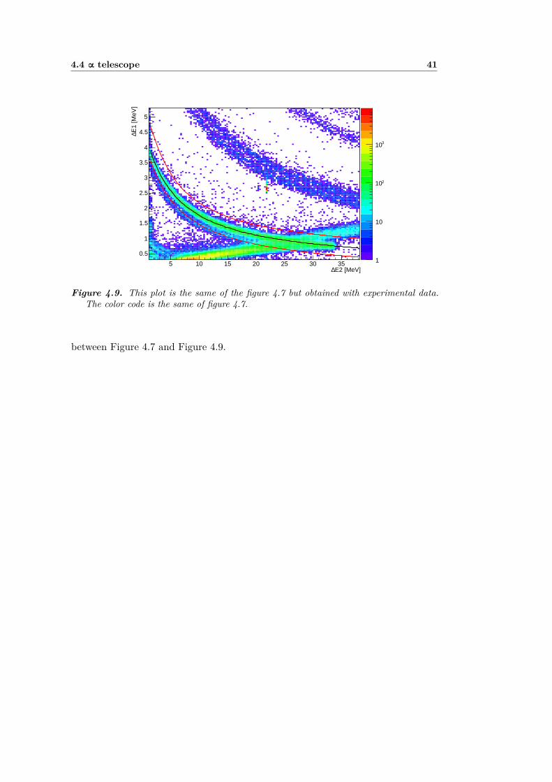
4.4 α telescope 41
E2 [MeV]∆5 10 15 20 25 30 35
E1
[MeV
]∆
0.5
1
1.5
2
2.5
3
3.5
4
4.5
5
1
10
210
310
Figure 4.9. This plot is the same of the figure 4.7 but obtained with experimental data.The color code is the same of figure 4.7.
between Figure 4.7 and Figure 4.9.

42 4. Data Analysis
) [MeV]αNaI (20 40 60 80 100 120 140 160 180 200 220
E2
[E M
eV]
∆
5
10
15
20
25
30
35
1
10
210
310
410
Figure 4.10. Energy deposition in the the ∆E2 as a function of the subsequent NaI. Datafrom the MC simulation. The black line is the expected energy deposition from α. Thered line delimits the selected region.
) [MeV]αNaI (20 40 60 80 100 120 140 160 180 200 220
E2
[E M
eV]
∆
5
10
15
20
25
30
35
1
10
210
310
410
Figure 4.11. As in figure 4.10 the plot shows the response of ∆E2 as a function of theNaI but here only the energy deposition due to the α’s is taken into account. The colorcode is the same of figure 4.10
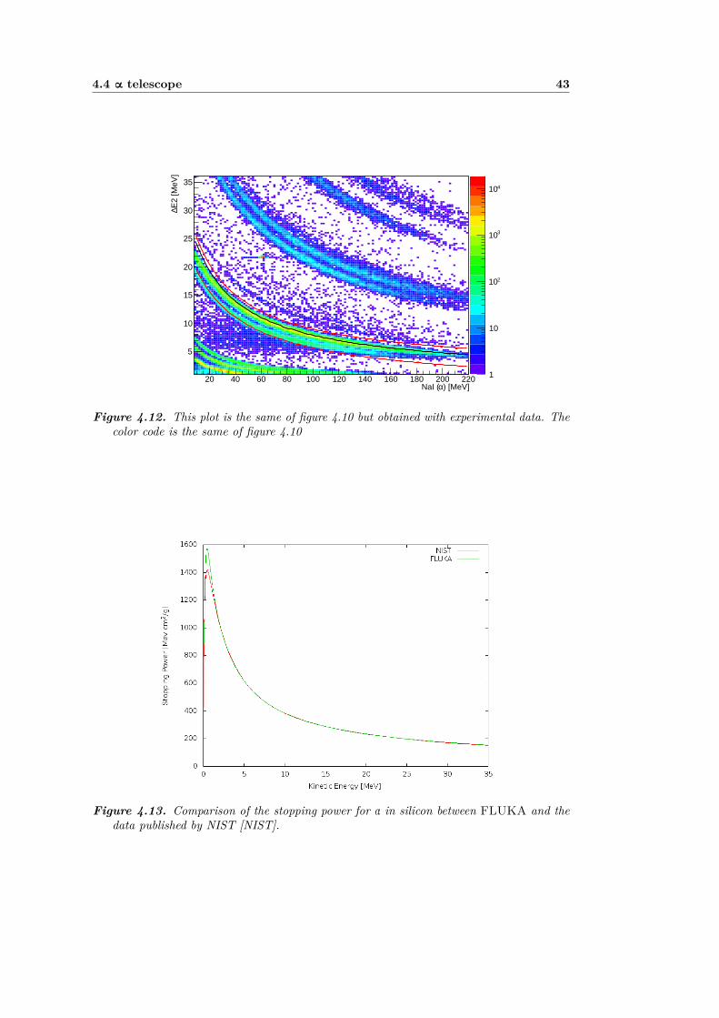
4.4 α telescope 43
) [MeV]αNaI (20 40 60 80 100 120 140 160 180 200 220
E2
[MeV
]∆
5
10
15
20
25
30
35
1
10
210
310
410
Figure 4.12. This plot is the same of figure 4.10 but obtained with experimental data. Thecolor code is the same of figure 4.10
Figure 4.13. Comparison of the stopping power for α in silicon between FLUKA and thedata published by NIST [NIST].

44 4. Data Analysis
4.4.1 Selection of 4He
As seen in the previous section, since the ∆E/E selection does not suffice to removethe contamination from 3He in the α telescope, another selection criterion has beenadded and it is described in this section.
The range (R) in the continus slowing down approximation of a charged particlecan be calculated integrating the total energy-loss (equation 1.3):
R =∫ 0
E0
(dE
dx
)−1dE (4.4)
where E0 is the initial energy of the particle. The integral in Equation 4.4 can besplit in to two terms:∫ 0
E0
(dE
dx
)−1dE =
∫ E′
E0
(dE
dx
)−1dE +
∫ 0
E′
(dE
dx
)−1dE (4.5)
the first term on the right side is the thickness (ε) where the particle loses an energy∆E = E0 − E′:
ε =∫ E′
E0
(dE
dx
)−1dE , (4.6)
i.e. it represents the passing through detector in the PID plot, while the secondterm in the equation 4.5 is the residual of the range of the particle in the stoppingdetector, where the particle loses the rest of its energy.
For a given particle and material the range R is function only of the energy:
R = f(E) , (4.7)
therefore it is possible to write the equation 4.5 as [VGTC67]:
f(E0) = ε+ f(E′) (4.8)
or:ε = f(∆E + E′)− f(E′) . (4.9)
In a restricted domain of energies, up to about 1 GeV for α particles (figure 4.14),f(E) can be approximated as:
f(E) ≈ kEn (4.10)
where k is a parameter, function of the mass and the charge of the particle, and n isa constant. From equation 1.6 it is possible to see that dE/dx should be proportionalto 1/β2, but as seen in figure 4.14, the energy-loss in the low energy region is betterapproximated by 1/β
53 [PDG98]. The value 5
3 is a phenomenological recipe and isdue to the onset of the shell corrections. For velocities much smaller than the speedof light, the energy is proportional to β2, so dE/dx ∝ 1/E
56 from which f(E) ∝ E
116 ,
therefore n ≈ 1.8. However, this value is obtained with many approximations andusing the data of the range in silicon published on [NIST] it is possible to obtaina more accurate value from a fit (figure 4.15). The value obtained from the fit is:n = 1.722± 0.002.
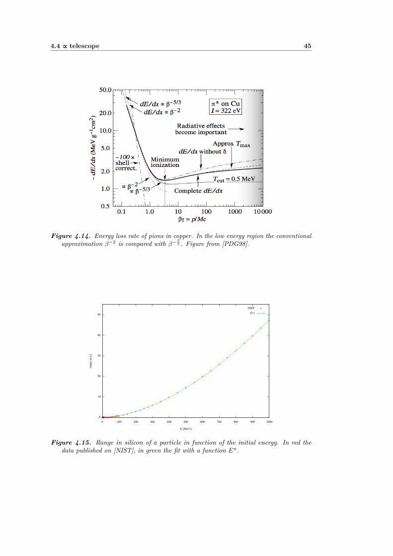
4.4 α telescope 45
Figure 4.14. Energy loss rate of pions in copper. In the low energy region the conventionalapproximation β−2 is compared with β− 5
3 . Figure from [PDG98].
Figure 4.15. Range in silicon of α particle in function of the initial energy. In red thedata published on [NIST], in green the fit with a function En.

46 4. Data Analysis
Using the approximation 4.10, equation 4.9 can be rewritten as:ε
k= (∆E + E′)n − (E′)n . (4.11)
Equation 4.11 is a function only of the characteristics of the particle and can beused to distinguish between different species. To do that it is convenient to define a“mass function” [LMG79] as:
m.f.(E′,∆E) =[(E′ + ∆E
)n − (E′)n]·Ms +M0 (4.12)
where Ms is a slope factor to increase the scale and M0 an offset.Plotting the mass function as a function of E′, it is possible to distinguish
between the different isotopes and particles. See as an example figure 4.16, wherethe mass function, obtained using ∆E2 as a passing through and the subsequent NaIas stopping detector, as a function of the energy deposition in the latter is shown.
E [MeV]50 100 150 200 250 300
Mas
s F
unct
ion
[a.u
.]
3000
3500
4000
4500
5000
5500
6000
6500
7000
0
10
20
30
40
50
Figure 4.16. Mass function as a function of E′ obtained using ∆E2 as passing throughdetector and the subsequent NaI as stopping detector. As is is possible to see in figure4.16, the lower locus is due to the 3He while the higher to 4He. Plot made with MC data.
To compare experimental and MC data and to set the gate, an histogram withthe values of the mass function has been done and it is presented in figure 4.18, forthe first couple of detectors, and in figure 4.17 for the second one. In other wordsthese histograms are the projections on the y axes of the bi-dimensional plots similarto Figure 4.16
The MC fits well the trend of the data in the mass function made with ∆E2 andthe NaI (Figure 4.17). There is an asymmetry of the experimental data that is notmatched by the MC. It could be due to the non perfect simulation of the quenchingin the low energy region, as can be seen comparing Figure 4.16 and Figure 4.19.Indeed there are no experimental points in the low energy region that could let torefine the simulation of the nonlinearitiy of the response of the NaI to low energyα’s.
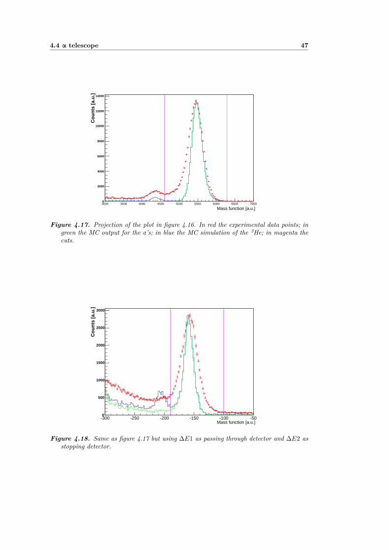
4.4 α telescope 47
Mass function [a.u.]3000 3500 4000 4500 5000 5500 6000 6500 7000
Co
un
ts [
a.u
.]
0
2000
4000
6000
8000
10000
12000
14000
Figure 4.17. Projection of the plot in figure 4.16. In red the experimental data points; ingreen the MC output for the α’s; in blue the MC simulation of the 3He; in magenta thecuts.
Mass function [a.u.]-300 -250 -200 -150 -100 -50
Co
un
ts [
a.u
.]
0
500
1000
1500
2000
2500
3000
Figure 4.18. Same as figure 4.17 but using ∆E1 as passing through detector and ∆E2 asstopping detector.

48 4. Data Analysis
E [MeV]50 100 150 200 250 300
Mas
s F
unct
ion
[a.u
.]
3000
3500
4000
4500
5000
5500
6000
6500
7000
0
50
100
150
200
250
300
350
Figure 4.19. Same as Figure 4.16 but made with experimental data.
An example of the mass function computed with ∆E1 as passing through detectorand ∆E2 as stopping detector is shown in Figure 4.18. The mass function calculatedwith experimental data has a larger distribution than the one calculated with MCdata. This could be due to the poorer resolution of the ∆E1. Unfortunately, it isnot possible to select, in the available data, something with an energy deposition inthe ∆E1 narrow enough to estimate its resolution.
4.5 Identification of possible contamination in the tar-get
In order to extract the cross-section of the quasi-elastic break up of 12C to 8Be andα, a two-dimensional energy spectra has been realised. Figure 4.20 shows the spectrawith the kinetic energy measured in the 8Be telescope as a function of the energymeasured in the α telescope. This plot refers to experimental data on C target. Thedata exhibit a doubly peak structure in the high energy region. To better visualisethis structure, and also to better identify the quasi-elastic peak, from now on thetwo-dimensional spectra will be displayed with the total energy as a function of theα energy. For instance, the same data of figure 4.20 are shown in figure 4.21, wherethe two peaks structure is even more evident. Those two peaks do not appear in theMC simulation, when only the C contribution is taken into account (figure 4.22).Another surprising feature shows up in the spectra of the α fragments, figure 4.27.Indeed the data show an excess in the high energy region, as if the α fragmentsspeed were greater than the original speed of the 12C projectile.
For these reasons, a contamination of Hydrogen has been supposed. To investigatethis hypothesis and emphasise the contribution of H, a dedicated experimental runwith a polyethylene (CH2)n target has been done. The experimental spectrum isshown in figure 4.23.
Simulating selectively several intermediate states of the interaction between C

4.5 Identification of possible contamination in the target 49
E [MeV]α0 50 100 150 200 250 300 350 400
Be
E [
MeV
]
0
50
100
150
200
250
300
350
400
0
5
10
15
20
25
30
Figure 4.20. Energy spectrum obtained from experimental data with the energy measuredin the 8Be telescope as a function of the energy measured in the α telescope. Target in C.
E [MeV]α0 50 100 150 200 250 300 350 400
+ B
e E
[M
eV]
α
0
100
200
300
400
500
600
0
5
10
15
20
25
30
Figure 4.21. Same as Figure 4.20 but with the sum of the energy measured in the twotelescopes as a function of the energy measured in the α one.

50 4. Data Analysis
E [MeV]α0 50 100 150 200 250 300 350 400
+ B
e E
[M
eV]
α
0
100
200
300
400
500
600
0
2
4
6
8
10
12
14
Figure 4.22. Same plot as in figure 4.21 but obtained with MC data.
E [MeV]α0 50 100 150 200 250 300 350 400
+ B
e E
[M
eV]
α
0
100
200
300
400
500
600
0
0.1
0.2
0.3
0.4
0.5
0.6
0.7
0.8
Figure 4.23. Same plot as in figure 4.21 but obtained with experimental data with a (CH2)ntarget.

4.5 Identification of possible contamination in the target 51
and H, it comes out that the experimental data can be explained by the reactionchannel in witch the 12C projectile, interacting with the H, produces a 9Bgs and acorrelated α. This reaction, in the frame where the C is at rest, is a (p,α) reaction, inwhich the proton is impinging on the C and an α particle is emitted. More details onthis reaction will be given in section 5.1. The 9Bgs subsequently decays in 8BeGS plusa proton. The double peak structure is due to the fact that sometimes the proton isdetected and enters in the selection. The high energy peak is produced when theproton goes in and its energy is added to the energy of the two α’s. The lower peakis produced when the proton is not detected. The events from this process that fitthe geometry of the experiment and the selection criteria are the ones in which theα is emitted, in the projectile rest frame, at large angles and this explains also theincreased energy of this fragment.
E [MeV]α0 50 100 150 200 250 300 350 400
+ B
e E
[M
eV]
α
0
100
200
300
400
500
600
0
10
20
30
40
50
60
70
80
90
Figure 4.24. Energy spectrum of the production of 9B and α in the interaction of a Cion with H. Histogram made with the total energy measured as a function of the energydeposited in the α telescope. MC simulation.
This reaction was already present in FLUKA, but just as one of the possiblechannels for the Fermi break-up and not as a pre-equilibrium reaction. A directmechanism has be added (it is described in the section 5.1) and the results are shownin Figures 4.24, 4.25, 4.26 and 4.27. Figure 4.24 shows the contribution to thebi-dimensional spectrum of the events with a production of 9Bgs, it is possible tosee the two sharp peaks structure. Figure 4.25 shows the FLUKA result for the(CH2)n target after the implementation of the (p,α) reaction in the pre-equilibriumstage. The contribution of the 9Bgs production is even more evident in Figures 4.26and 4.27, that are the projections on the two axis of the bi-dimensional spectra inFigurs4.25 and 4.23.
As said in chapter 3, the MC simulate the direct interaction between the beamand the target atoms, therefore the simulation of the (CH2)n target has been doneseparately for the H and C contribution and summed up, and confronted with

52 4. Data Analysis
E [MeV]α0 50 100 150 200 250 300 350 400
+ B
e E
[M
eV]
α
0
100
200
300
400
500
600
0
0.1
0.2
0.3
0.4
0.5
0.6
0.7
0.8
Figure 4.25. Same as Figure 4.23 but with MC data.
+ Be E [MeV]α0 100 200 300 400 500 600
MeV
]2
dE
[m
b /
sr2
Ω /
dσ 3 d
0
0.5
1
1.5
2
2.5
3
3.5
4
4.5
Figure 4.26. Projection on the total energy axis of the plot in Figure 4.25. In red theexperimental data; in black the total MC spectrum, in green the part due to the H and inblue its part that produced 9B as intermediate state. In magenta the part due to C.

4.6 Evaluation of the Hydrogen contamination 53
E [MeV]α0 50 100 150 200 250 300 350 400
MeV
]2
dE
[m
b /
sr2
Ω /
dσ 3 d
0
0.5
1
1.5
2
2.5
3
Figure 4.27. Same as Figure 4.26 but for the α telescope axis.
experimental data, multiplying each output by a scaling factor:
sfH =σ(C,H)
Nprim(H)1302 (4.13)
sfC =σ(C,H)
Nprim(C)130 (4.14)
where Nprim is the number of primaries simulated in each simulation, σH and σCare the total inelastic cross sections of C on H and C atoms, the factor 1
30 is due tothe biasing introduced by the rotation of the events (cfr. section 3.1) and the factor2 in Equation 4.13 is due to the stoichiometric ratio.
4.6 Evaluation of the Hydrogen contamination
As seen in the previous section, the hypothesis of a H contamination in the targetswith the production of 9B explains the double peak structure and the excess ofhigh energy α’s. However the amount of H in each target is unknown, with theexception of the (CH2)n target. In order to evaluate this amount and to verify theangular distribution of the 9B production, the selection criteria have been modifiedto insulate the events in which 9B has been produced. Three firing strips havebeen requested. Two of these strips have to fit in the selection criteria described insection 4.3, to identify the two α’s; the third one has to measure an energy depositionsmaller than 1.5 MeV, the energy deposition expected from the Proton emitted inthe 9B decay in Proton and 8Be. In this way only the events where the Proton andthe two α’s coming from the decay of a 9Bgs hit the SSD in three different strips areselected.

54 4. Data Analysis
4.6.1 Angular distribution of the Boron production
Figure 4.28 shows the cross section of the reaction 12C + p −−→ 9B + α in thelaboratory frame when the 9B is emitted in the angular acceptance of the Betelescope as a function of the angle of emission of the α fragment.
This cross section increases with the angle of emission of the α fragment andsuddenly drops after 22. This characteristic is due to the Lorentz transformationfrom the Carbon rest frame and the laboratory frame. The cross section drops after22 because this is the limit angle, as will be discussed in subsection 5.1.1.
There is a good agreement between MC and experimental data, especially at 16where the statistic is higher. For the other angles the MC seems overestimate theproduction and the resolution of the Be telescope seems narrower, reflecting in anarrower peak in the total energy. Figure 4.28 shows the cross section calculatedwith FLUKA of the 12C + p −−→ 9B + α reaction with the 9B emitted in the range9 ± 3, the acceptance of the Be telescope, as a function of the emission angle ofthe α.
[deg.]αΘ8 10 12 14 16 18 20 22 24
]2
[mb
/ deg
.α
Θ /
dB
eΘ
/ d
σ 2 d
-310
-210
-110
1
10
Figure 4.28. Cross section of the 12C + p −−→ 9B + α reaction with the 9B emitted in therange 9 ± 3 as a function of the emission angle of the α.
Figures 4.29 to 4.33 show the total energy deposited and the energy measuredin the α telescope for its different positions taken with the (CH2)n target. As it ispossible to see from the MC histograms in these plots, the contribution from the Cin the target is almost completely rejected from the three firing strips requirementand practically only the events with a 9B as intermediate state are selected.

4.6 Evaluation of the Hydrogen contamination 55
+ Be E [MeV]α0 100 200 300 400 500 600
MeV
]2
dE
[m
b /
sr2
Ω /
dσ 3 d
0
1
2
3
4
5
(a)
E [MeV]α0 50 100 150 200 250 300 350 400
MeV
]2
dE
[m
b /
sr2
Ω /
dσ 3 d
0
0.2
0.4
0.6
0.8
1
1.2
1.4
1.6
1.8
2
2.2
(b)
Figure 4.29. (a) Energy deposited in the two telescopes selecting events with 3 firing stripsand using a (CH2)n target and with the α telescope at 16. In red the experimental data,in green the H contribution and in blue the events on H that produced a 9B. (b) Same as(a) but for the α telescope. The contribution from the C is in magenta and it is visibleonly in the low energy region of this plot.
+ Be E [MeV]α0 100 200 300 400 500 600
MeV
]2
dE
[m
b /
sr2
Ω /
dσ 3 d
0
1
2
3
4
5
(a)
E [MeV]α0 50 100 150 200 250 300 350 400
MeV
]2
dE
[m
b /
sr2
Ω /
dσ 3 d
0
0.5
1
1.5
2
2.5
3
3.5
(b)
Figure 4.30. Same as 4.29 but with the α telescope placed at 18.

56 4. Data Analysis
+ Be E [MeV]α0 100 200 300 400 500 600
MeV
]2
dE
[m
b /
sr2
Ω /
dσ 3 d
0
2
4
6
8
10
(a)
E [MeV]α0 50 100 150 200 250 300 350 400
MeV
]2
dE
[m
b /
sr2
Ω /
dσ 3 d
0
1
2
3
4
5
(b)
Figure 4.31. Same as 4.29 but with the α telescope placed at 20.
+ Be E [MeV]α0 100 200 300 400 500 600
MeV
]2
dE
[m
b /
sr2
Ω /
dσ 3 d
0
5
10
15
20
25
30
35
(a)
E [MeV]α0 50 100 150 200 250 300 350 400
MeV
]2
dE
[m
b /
sr2
Ω /
dσ 3 d
0
2
4
6
8
10
12
(b)
Figure 4.32. Same as 4.29 but with the α telescope placed at 22.
+ Be E [MeV]α0 100 200 300 400 500 600
MeV
]2
dE
[m
b /
sr2
Ω /
dσ 3 d
0
0.02
0.04
0.06
0.08
0.1
0.12
0.14
0.16
0.18
0.2
(a)
E [MeV]α0 50 100 150 200 250 300 350 400
MeV
]2
dE
[m
b /
sr2
Ω /
dσ 3 d
0
0.05
0.1
0.15
0.2
0.25
0.3
(b)
Figure 4.33. Same as 4.29 but with the α telescope placed at 24.

4.6 Evaluation of the Hydrogen contamination 57
4.6.2 Evaluation of the H contamination in the targets
As seen in the previous section, the C contribution in the data related to the (CH2)ntarget completely disappears with the selection criteria described in it. This meansthat it is possible to select only the H contribution in the data taken with theother targets. Comparing the (CH2)n experimental data with the experimentaldata taken with each other targets, it is possible to estimate the amount of H thatcontaminates each target. Therefore, for every target and every position of the αtelescope, the data have been compared with the data relative to (CH2)n target.The contamination of H has been calculated imposing the same integral for the twohistograms. Figures 4.34 show the data relative to the Au target. Figures 4.36 arethe same for the Nb target and 4.35 for the C target. For Au, the data have notbeen acquired with the α telescope placed at 22, while for Nb, unfortunately, thedata relative to the α placed from 18 to 22 have been corrupted (probably duringthe first step of the conversion of the data files).
The contaminations calculated for each target with the α telescope placed ineach position are summarised in Table 4.2 and shown in Figure 4.37. For Au and Ctargets, a weighted average has been calculated. They are indicated by the greenline in Figure 4.37 and summarised in Table 4.3.
Table 4.2. Estimated H contamination for each run matching the aerea of each histogramswith the corresponding one taken with (CH2)n target.
Target angle contamination[deg.] [µg/cm2]
Au 16 2.1± 0.2Au 18 2.4± 0.3Au 20 0.6± 0.1Nb 16 3.8± 0.4C 16 79± 5C 18 170± 12C 20 18± 2C 22 17± 2
Table 4.3. Average H contamination for Au and C targets.
Target contamination[µg/cm2]
Au 1.1± 0.5C 22± 1
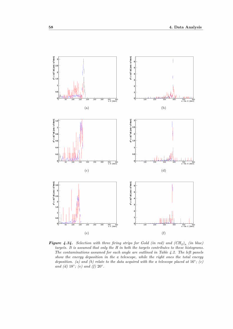
58 4. Data Analysis
E [MeV]α0 50 100 150 200 250 300 350 400
MeV
]2
dE
[m
b /
sr2
Ω /
dσ 3 d
0
0.5
1
1.5
2
2.5
3
(a)
+ Be E [MeV]α0 100 200 300 400 500 600
MeV
]2
dE
[m
b /
sr2
Ω /
dσ 3 d
0
1
2
3
4
5
6
(b)
E [MeV]α0 50 100 150 200 250 300 350 400
MeV
]2
dE
[m
b /
sr2
Ω /
dσ 3 d
0
0.2
0.4
0.6
0.8
1
1.2
(c)
+ Be E [MeV]α0 100 200 300 400 500 600
MeV
]2
dE
[m
b /
sr2
Ω /
dσ 3 d
0
0.5
1
1.5
2
2.5
3
(d)
E [MeV]α0 50 100 150 200 250 300 350 400
MeV
]2
dE
[m
b /
sr2
Ω /
dσ 3 d
0
0.5
1
1.5
2
2.5
3
3.5
(e)
+ Be E [MeV]α0 100 200 300 400 500 600
MeV
]2
dE
[m
b /
sr2
Ω /
dσ 3 d
0
1
2
3
4
5
6
(f)
Figure 4.34. Selection with three firing strips for Gold (in red) and (CH2)n (in blue)targets. It is assumed that only the H in both the targets contributes to these histograms.The contaminations assumed for each angle are outlined in Table 4.2. The left panelsshow the energy deposition in the α telescope, while the right ones the total energydeposition. (a) and (b) relate to the data acquired with the α telescope placed at 16; (c)and (d) 18; (e) and (f) 20.
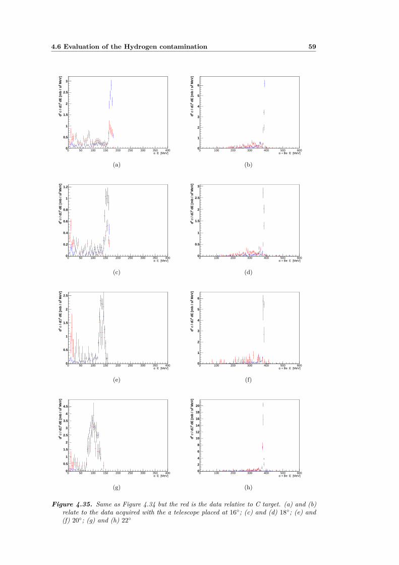
4.6 Evaluation of the Hydrogen contamination 59
E [MeV]α0 50 100 150 200 250 300 350 400
MeV
]2
dE
[m
b /
sr2
Ω /
dσ 3 d
0
0.5
1
1.5
2
2.5
3
(a)
+ Be E [MeV]α0 100 200 300 400 500 600
MeV
]2
dE
[m
b /
sr2
Ω /
dσ 3 d
0
1
2
3
4
5
6
(b)
E [MeV]α0 50 100 150 200 250 300 350 400
MeV
]2
dE
[m
b /
sr2
Ω /
dσ 3 d
0
0.2
0.4
0.6
0.8
1
1.2
(c)
+ Be E [MeV]α0 100 200 300 400 500 600
MeV
]2
dE
[m
b /
sr2
Ω /
dσ 3 d
0
0.5
1
1.5
2
2.5
3
(d)
E [MeV]α0 50 100 150 200 250 300 350 400
MeV
]2
dE
[m
b /
sr2
Ω /
dσ 3 d
0
0.5
1
1.5
2
2.5
(e)
+ Be E [MeV]α0 100 200 300 400 500 600
MeV
]2
dE
[m
b /
sr2
Ω /
dσ 3 d
0
1
2
3
4
5
6
(f)
E [MeV]α0 50 100 150 200 250 300 350 400
MeV
]2
dE
[m
b /
sr2
Ω /
dσ 3 d
0
0.5
1
1.5
2
2.5
3
3.5
4
4.5
(g)
+ Be E [MeV]α0 100 200 300 400 500 600
MeV
]2
dE
[m
b /
sr2
Ω /
dσ 3 d
0
2
4
6
8
10
12
14
16
18
20
(h)
Figure 4.35. Same as Figure 4.34 but the red is the data relative to C target. (a) and (b)relate to the data acquired with the α telescope placed at 16; (c) and (d) 18; (e) and(f) 20; (g) and (h) 22
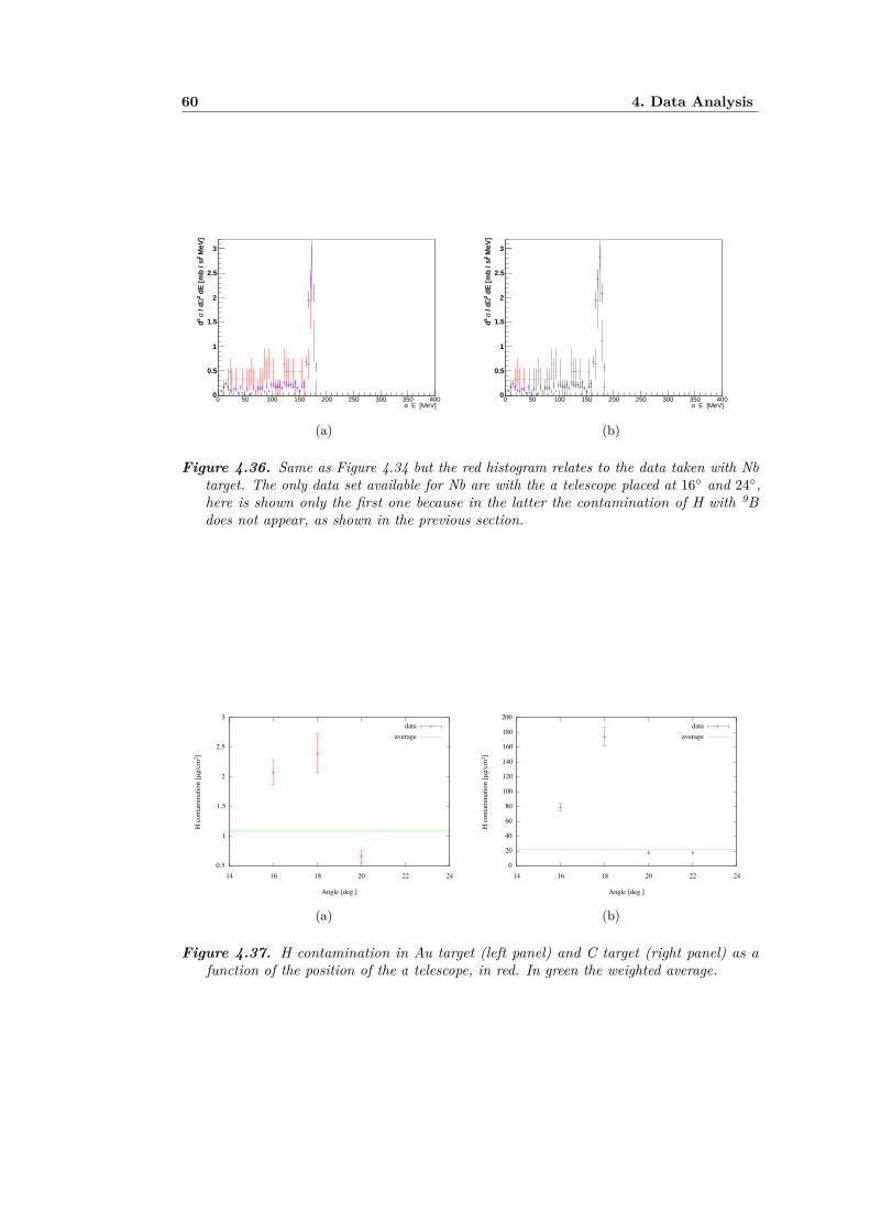
60 4. Data Analysis
E [MeV]α0 50 100 150 200 250 300 350 400
MeV
]2
dE
[m
b /
sr2
Ω /
dσ 3 d
0
0.5
1
1.5
2
2.5
3
(a)
E [MeV]α0 50 100 150 200 250 300 350 400
MeV
]2
dE
[m
b /
sr2
Ω /
dσ 3 d
0
0.5
1
1.5
2
2.5
3
(b)
Figure 4.36. Same as Figure 4.34 but the red histogram relates to the data taken with Nbtarget. The only data set available for Nb are with the α telescope placed at 16 and 24,here is shown only the first one because in the latter the contamination of H with 9Bdoes not appear, as shown in the previous section.
(a) (b)
Figure 4.37. H contamination in Au target (left panel) and C target (right panel) as afunction of the position of the α telescope, in red. In green the weighted average.

61
Chapter 5
Monte Carlo implementation
This chapter describe of the models implemented in FLUKA to simulate theinteractions relevant to simulate the experiment. We will firstly go in the detail ofthe (p,α) reaction hypothesised to understand the double peak structure describedin section 4.5 and then we will describe the implementation of such interaction asa pre-equilibrium emission of the α, because this process was already implementedin FLUKA but only as one of the Fermi break-up possible channels. The secondsection describes the implementation of the quadrupole electromagnetic interaction,that has been done because it could simulate the quasi-elastic break-up of C ions.
5.1 Proton-alpha reactions in nucleiA (p, α) reaction is an interaction where a proton collide with a nucleus and an αparticle is emitted:
p+ x→ a+ x′ (5.1)In the case in exam we have a 12C ion impinging on a H target and an α particle
emitted in the laboratory frame with an angle θ fixed, defined by the position of theα telescope.
12C + H→ 4He + 9BGS (5.2)In the laboratory frame the invariant mass
√s is:
s = M2C +M2
H + 2ECMH (5.3)
while in the center of mass frame (CM) it is:
s = (E?He + E?B)2 (5.4)
from which:E?B =
√s− E?He . (5.5)
Equating the relation between energy, mass and momentum, namely:
E?B =√p?B
2 +M2B , (5.6)
to Equation 5.5, it is possible to obtain:
p?B2 +M2
B = s+ E?He2 − 2
√sE?He (5.7)

62 5. Monte Carlo implementation
and finally the energy of the α fragment in the CM frame:
E?He = s+M2He −M2
B2√s
. (5.8)
To calculate the energy of the other fragment, E?B, it is possible to use the relation5.5.
To impose the angle of emission of one fragment in the laboratory frame it issimpler to calculate the transformation from this frame to the CM:
E?He = γ [EHe − βpHe cos(θ)] (5.9)
which is equivalent to:
γEHe = E?He + ηpHe cos(θ) (5.10)
where η = βγ. Substituting in 5.10 the energy of the α in the laboratory frame:
EHe =√pHe2 +M2
He (5.11)
it is possible to obtain:
[E?He + ηpHe cos(θ)]2 = γ2(pHe
2 +M2He
)(5.12)
and carrying out the square:
E?He2 + η2p2
He cos2(θ) + 2ηE?HepHe cos(θ) = γ2p2He + γ2M2
He (5.13)
from which, using the equivalence γ2 − η2 = 1 and rearranging the terms, it ispossible to write:[
1 + η2 sin2(θ)]p2
He − 2 [ηE?He cos(θ)] pHe +[η2M2
He − p?He2]
= 0 (5.14)
Solving the equation 5.14 for pHe:
pHe =ηE?He cos(θ)±
√[ηE?He cos(θ)]2 −
[1 + η2 sin2(θ)
]·[η2M2
He − p?He2]
1 + η2 sin2(θ). (5.15)
Equation 5.15 has two possible solutions for the argument of the square root greaterthan zero, as appear also in Figure 5.1(a), where is shown the energy of the α infunction of its emission angle, both in the laboratory frame. Nonetheless, only oneof the two possible solutions matches the acceptance of the detector: in fact theangle of emission of the other fragment - the 9B - has to be in the acceptance ofthe 8Be telescope. As emerges in 5.1(d), where the angle of emission of 9B as afunction of the one of the α is shown, only one of the two solutions respects thisrequirement. Furthermore, the plot shows that for the α angle of emission between16 and the largest kinematically possible one, the 9B angle is always in the range8÷ 10, the acceptance of the 8Be telescope. When the argument of the square rootin Equation 5.15 is zero, the two solutions coincides and this defines the maximum

5.1 Proton-alpha reactions in nuclei 63
emission angle. Going back to 5.1(c), this plot highlights also the energy dependenceof the α as a function of the angle in the laboratory frame, reflecting the featureof the experiment. Figure 5.1(b) shows the energy of the 9B fragment again as afunction of the emission angle of the α, from a comparison of this plot and the onein Figure 5.1(a) it is possible to understand why in the experimental data the αseems to subtract energy to the other fragments. Finally, in Figure 5.1(c) is shownthe α angle in the C rest frame as a function of the α angle in the laboratory frame,and from this plot emerges that the detected α’s are the those emitted with at largeangle in the C rest frame.
5.1.1 Angular kinematics
The angular kinematics of the α’s emitted in the (p,α) reaction can be calculatedfrom geometrical considerations: in the CM frame the spectrum of the possiblemoduli of the momenta of the α particles, p?, is in a diagram px − pz a circle ofradius p? where the angle in the plane it is the diffusion angle θ?:
p?x2
p?2 + p?z2
p?2 = 1 (5.16)
In a generic reference frame boosted along the Z axis, and then also in the laboratoryframe, the components of the momentum of one of the two particles is:
px = p?x (5.17)pz = γ (p?z + βE?) (5.18)
where β is the speed of the CM frame in the other reference frame, and γ = (1−β2)−12 .
Using the equations 5.17 in the equation 5.16 it is possible to obtain:
px2
p?2 + (pz − βγE?)2
γ2p?2 = 1 (5.19)
which is the equation of an ellipse centred in pz = βγE?. From this equation it isalso possible to see the reason of the two possible solutions, indeed, for a given θ inthe range 0÷ θmax there are two intersections between the ellipse and a straight linestarting in the origin with an angle θ respect to the Z axis. If θ = θmax the line istangent to the ellipse, and the two solutions coincide, while for θ above θmax theline does not intersect the ellipse anymore and there are no possible solutions.
To find θmax it is possible to write the relation between the angle in the laboratoryframe and the angle of emission in the CM frame:
tan(θ) = pxpz
= p?xγ(p?z + βE?) = sin(θ?)
γ[cos(θ?) + βE
?
p?
] (5.20)
since tan(θ) is a monotone function of θ, the maximum of the latter is also amaximum in the first one, hence taking derivative of the Equation 5.20:
d tan(θ)dθ?
=βE
?
p? cos(θ?) + 1γ[cos(θ?) + βE
?
p? ]2(5.21)

64 5. Monte Carlo implementation
(a) (b)
(c) (d)
Figure 5.1. Energy in the laboratory frame of the α (a) and of the 9B (b) as a functionof the α angle in the laboratory. (c) Angle of emission of the α fragment in the C restframe as a function of its angle in the laboratory frame. (d) Angle of emission of the 9Bin the laboratory frame as a function of the α angle. In all these plots in red is shownthe first solution and in green the second one.

5.2 The Electro-Magnetic dissociation 65
and imposing it equal to zero it is possible to find the cosine of the angle in the CMthat correspond to the maximum angle in the laboratory frame:
cos(θ?) = − 1β
p?
E?. (5.22)
Finally to calculate θmax, it is possible to use Equation 5.22 in Equation 5.20:
tan(θmax) =
√1− ( 1
βp?
E? )2
γ[βE
?
p? − 1βp?
E?
] (5.23)
which gives θmax = 22.0631 consistent with Figure 5.1(c).
5.1.2 Implementation in FLUKA
The collision of the C ion on the proton creates an excited state that could emit anα in the pre-equilibrium stage treated in the PEANUT model. This pre-equilibriumemission of an α due to a (p,α) reaction has been added to FLUKA. It works in asimilar way of the pre-equilibrium emission in the continuum of nucleon (introducedin section 1.7). To the nucleon emission probability has been added a preformationfactor for he α’s, which is 0.2 in the low energy domain and tends to zero for higherenergies, i.e. greater than the binding energy of the α particles. The initial numberof excitons is three: two particle like and an hole, due to the interaction of theimpinging p with the nucleus. To emit the α the nucleon-nucleon interaction chainhas to produce at least four particle like excitons and two has to be neutrons andtwo protons, therefore at least three holes are produced. Finally, the energy of theemitted α is calculated subtracting to the total available energy the one taken bythe three holes as sampled from the energy partition function.
5.2 The Electro-Magnetic dissociationAs already mentioned in Section 1.5, one of the possible kinds of interaction thatleads to the break-up of the projectile nucleus is the electromagnetic dissociation.When the impact parameter is greater than the sum of the radii of the nuclei(b > Rp + Rt), there is no overlap between the two nuclear density. However, theelectromagnetic field is so high that it provokes the excitation, and eventually thebreak-up of one or of even both of the nuclei.
The simplest way to describe this reaction mechanism is provided by the equiv-alent photon method, also commonly referred to as Weizsäcker-Williams method[Jac62]. It is based on the fact that an incident particle with charge Zpe, mass Mand energy E produces the same effect as a beam of photons with a spectrum ρ(ω)given, in the leading logarithmic approximation [BHTS02], by:
napp.(ω) = 2Z2pα
πβ2 ln(
γ
ωRp
)(5.24)
where ω is the photon energy, Rp the projectile nucleus radius, α is the fine structureconstant, β is the speed of the particle and γ is the Lorentz factor.

66 5. Monte Carlo implementation
Therefore, the cross section of electromagnetic dissociation (σEMD) can bewritten factoring it into the equivalent photon spectrum 5.24 and the photo-nuclearcross section for (quasi) real photons σγ(ω):
σEMD =∫ ωmax
ωmin
dω
ωn(ω)σγ(ω) (5.25)
where ωmin is the threshold energy of the photon that can cause a single nucleonemission and ωmax ≈ γ/Rp.
The PEANUT event generator used in FLUKA (see Section 1.6) uses this modelto describe the electromagnetic dissociation induced by the absorption of both realand virtual photons [BFF+14].
At relativistic energies, the field of quasireal photons contains all the multi-polarities with the same weight. However, since the cross section of the electricdipole (σγE1) is the dominant one, it was considered a good approximation to takeinto account only the contribution from E1 virtual photons [BFF+14]. On thecontrary, at low speeds the calculation of the photonuclear cross section should bedone summing the contributions from all the multipolarities. Nevertheless, onlya few of them contribute in most processes [BB88]. Namely, the three dominantmultipolarities are the electric dipole, the quadrupole (E2) and the magnetic dipole(M1). The electromagnetic dissociation cross section 5.25 can be rewritten as:
σEMD =∫ ωmax
ωmin
dω
ω
[nE1(ω)σγE1(ω) + nE2(ω)σγE2(ω) + nM1(ω)σγM1(ω)
](5.26)
At low energies, the E2 photon spectrum dominates and σγE2 is its maximum in thelow energy region (Figure 5.2), hence the quadrupole interaction plays an importantrole in low energy interactions. This contribution has been added to FLUKA to
Figure 5.2. σγE1(ω), σγE2(ω) and σγM1(ω) in the interaction between 40Ca with 238U asa function of the laboratory energy per nucleon. Plot from [BB88].
verify if it could add a significant contribution for the break-up of C ions in theenergy region of interest.

5.2 The Electro-Magnetic dissociation 67
The flux of virtual photons nE1(ω) is:
nE1(ω) = 2πZ2p
α
β2
[ζK0K1 −
ζ2β2
2(K2
1 −K20
)](5.27)
while, nE2(ω) is:
nE2(ω) = 2πZ2p
α
β4
[2(1− β2
)K2
1 + ζ(2− β2
)2K0K1 −
ζ2β4
2(K2
1 −K20
)](5.28)
where K0 and K1 are the modified Bessel functions respectively of order zero andone, functions of the adiabaticity parameter ζ = ω(Rp +Rt)c/βγ. The increasing ofthe contribution of nE2(ω) compared to nE1(ω) in the small energy region respectto the high energy one is due to the its dependence to 1/β4, while nE1(ω) dependsto 1/β2.
The cross section σγE2(ω) is calculated following Prestwich et al. [PIK84] with aLorentzian:
σγE2(ω) = σ0Γ2Tω
2(ω2 − E2
T
)2 + Γ2Tω
2(5.29)
where σ0 is the peak cross section of the quadrupole resonance centred at energyET and width ΓT . σ0 has been calculated [PIK84] as:
σ0 = 25παR2
pA13p Z2
pE20
Mpc2ΓT= 0.14ZpA
23pE2
0 [MeV2]ΓT [MeV] [µb] (5.30)
Experimental data show the following dependency of ET from A [Kapecky]:
ET = A13 · 63 MeV (5.31)
and for ΓT [IAEA]ΓT = 6.11 MeV−A · 0.021 MeV (5.32)
Since the numerical integration of the nE1(ω)σγE1(ω) and nE2(ω)σγE2(ω) prod-ucts is very time consuming, the program uses an approximation to initially evaluatethe probability of an electromagnetic dissociation, and in case calculate exactlythe cross sections and the photon equivalent fluxes. For the initial estimation thephoton energy range is divided into intervals; σγ(ω) is approximated with Beziercurves, and the total equivalent photon spectrum is calculated in the leading orderapproximation as:
napp.(ω) = 2Z2α
πln(
γ
ωRp
)(5.33)
the product of the fit made with the Bezier curves and napp.(ω) is analyticallyintegrable and allows an overestimation of the total cross section σEMD. If theelectromagnetic interaction is selected, the program samples the photon energy ωand calculates the probability of the interaction to happen as the ratio of the crosssection exactly calculated for the selected ω and the approximated one:
P (ω) = nE1(ω)σγE1(ω) + nE2(ω)σγE2(ω)napp.(ω)σBezier(ω) (5.34)
68 5. Monte Carlo implementation
this technique allows fast estimation of the cross section for hundreds of nuclideswithout introducing any approximations.
After being excited, the nucleus can emit protons and neutrons before thethermalisation. Afterwards, the deexcitation proceeds through evaporation, fission,or, for light nuclei, Fermi break-up (Section 1.7.2). Parity and angular momentumconservation is taken into account according to the multipolarity selected for theinteraction.
Despite of the fact that for low energy the relevance of the E2 contributionis greater than the higher one, in the purpose of this work a preliminary analysisshowed that it did not give any significant contribution.

69
Chapter 6
Results
The experiment described in this work has been performed in order to measurethe cross section of the quasi-elastic break-up of Carbon ions into 8Be and α ondifferent materials. The doubly peak structure and the excess of α’s in the highenergy region have been attributed to a Hydrogen contamination in the targetsand to the production of 9Bgs out of the interactions of the Carbon ion beam withthe contaminant. This interaction has been added as a possible channel of thepre-equilibrium stage in FLUKA.
This chapter highlights the comparison of the cross section calculated withFLUKA with experimental data of α production in the interaction of Proton beamwith 16O target as well as the cross section of quasi-elastic breakup of 12C with thedifferent targets, limiting the impact of the H contamination.
6.1 Benchmark of the (p,α) reactionThe Figures 6.1 show the cross sections calculated with FLUKA for the inclusiveproduction of H, Deuterium and α particles in the interaction of a p beam with61.4 MeV with an 16O target. The experimental data are taken from [BP73]. The leftpanel shows the FLUKA output before the introduction of the α as a possible ejectile,as described in subsection 5.1.2, while the one on the right shows the same crosssection calculated after the implementation of the (p,α) reaction. As it is possible tosee comparing the two plots, FLUKA now reproduces accurately the high energypart of the α emission spectrum, the region where the pre-equilibrium emission of αparticles is more significant. This benchmark shows that the α preformation factorgives a total cross section for the (p,α) reaction compatible with experimental data,independently from the (CH2)n target data described in this work.

70 6. Results
(a) (b)
Figure 6.1. Comparison of the cross sections for (p,p) in green, (p,d) in blue and (p,α)in red before (left panel) and after (right panel) the implementation in FLUKA of theα as a possible ejectile of the pre-equilibrium stage. The histograms are the FLUKAcalculations while the dots are the experimental data points. Data from [BP73].

6.2 The 12C quasi-elastic break-up cross section 71
6.2 The 12C quasi-elastic break-up cross sectionTo limit the impact of Hydrogen, it is possible to modify the selection criteria,requiring not only at least two strips in the cuts described in section 4.3, but alsothat no more than two SSD strips fire. In this way, at least the events where theproton (coming from the decay of the 9B) is detected, are rejected. Figures 6.2 showthe total and the α telescope energy distribution related to (CH2)n target with theα telescope at 16. The higher peak in the total energy, the one where also theproton is entering in the detectors, is significantly reduced. The residual fractionof the peak is due to the protons that pass through the SSD frame and reach thesubsequent NaI.
+ Be E [MeV]α0 100 200 300 400 500 600
MeV
]2
dE
[m
b /
sr2
Ω /
dσ 3 d
0
2
4
6
8
10
12
14
16
18
20
(a)
E [MeV]α0 50 100 150 200 250 300 350 400
MeV
]2
dE
[m
b /
sr2
Ω /
dσ 3 d
0
2
4
6
8
10
(b)
Figure 6.2. Total (a) and α telescope (b) energy distributions obtained with the (CH2)ntarget and the α telescope at 16. In red the experimental data, in black the total MC; ingreen the total contribution of the H contamination and in blue the part of these where a9Bgs has been produced. In magenta the C contribution.
6.2.1 Niobium target
Figures 6.3 highlight the results for the data and MC related to Nb target and the αtelescope placed at 16. The contamination of H here is assumed to be 3.8 µg/cm2,as found in subsection 4.6.2.
From the projection on the two axis (Figures 6.3(c) and 6.3(d)) it is possibleto see that the contribution of the H contamination is considerable, neverthelessthe events due to the interaction with Nb can still be identified. Moreover, thequasi-elastic break-up of 12C in α and 8Be on Nb target peak is visible in Figure6.3(a) with total Energy in the range 367÷ 410 MeV. To better identify this peak itis possible to project on the α axis only the part of the bi-dimensional spectrum inthe total Energy range 367÷ 410 MeV. The result is shown in Figure 6.4. In thisplot the contribution of the H contamination is even more limited.
Unfortunately, the data relative to the Nb target, with the α telescope placedat 18, 20 and 22 have been corrupted. Except the data set with the α telescopeplaced at 16, the only one available relates to data acquired with the α telescopeplaced at 24. Figure 6.5 shows the results for this configuration, with the same gate

72 6. Results
0
0.05
0.1
0.15
0.2
0.25
0.3
E [MeV]α0 50 100 150 200 250 300 350 400
+ B
e E
[M
eV]
α
0
100
200
300
400
500
600
(a)
0
0.05
0.1
0.15
0.2
0.25
0.3
E [MeV]α0 50 100 150 200 250 300 350 400
+ B
e E
[M
eV]
α0
100
200
300
400
500
600
(b)
+ Be E [MeV]α0 100 200 300 400 500 600
MeV
]2
dE
[m
b /
sr2
Ω /
dσ 3 d
0
2
4
6
8
10
12
14
16
(c)
E [MeV]α0 50 100 150 200 250 300 350 400
MeV
]2
dE
[m
b /
sr2
Ω /
dσ 3 d
0
1
2
3
4
5
6
(d)
Figure 6.3. Bi-dimensional cross section on Nb target, with the α telescope at 16 fromexperimental data (a) and MC (b). In (c) their projection on the Y axis and in (d) theprojection on the X axis. In these two plots in red are shown the experimental data, inblack the total MC; in green the total contribution of the H contamination and in bluethe part of these where a 9Bgs has been produced. In magenta the C contribution.

6.2 The 12C quasi-elastic break-up cross section 73
E [MeV]α0 50 100 150 200 250 300 350 400
MeV
]2
dE
[m
b /
sr2
Ω /
dσ 3 d
0.5
1
1.5
2
2.5
3
3.5
Figure 6.4. Projection of the spectrum in Figure 6.3 on the α axis selecting only the eventswith total energy in the range 367÷ 410 MeV. α telescope placed at 16.
described before to insultate the quasi-elastic break-up in the data, since at suchangle the H contamination does not appear, for the kinematic reasons described insubsection 5.1.1.

74 6. Results
E [MeV]α0 50 100 150 200 250 300 350 400
MeV
]2
dE
[m
b /
sr2
Ω /
dσ 3 d
0.5
1
1.5
2
2.5
3
3.5
Figure 6.5. Same as Figure 6.4 but with the α telescope placed at 24.
6.2.2 Gold target
The same analysis performed on the Nb related data has been applied on Au data.The results are shown in Figures 6.6, while the projection on the α axis in the gateset to insulate the quasi-elastic peak is shown in Figure 6.7. Also in this case, thequasi elastic peaks due to the interaction with the target material can be identified.For this target, the data are available with the α telescope placed at 16 (Figure 6.7),18 (Figure 6.8), 20 (Figure 6.9) and 24 (Figure 6.10). A run with the a telescopeplaced at 22 was not done.

6.2 The 12C quasi-elastic break-up cross section 75
0
0.02
0.04
0.06
0.08
0.1
0.12
E [MeV]α0 50 100 150 200 250 300 350 400
+ B
e E
[M
eV]
α
0
100
200
300
400
500
600
(a)
0
0.02
0.04
0.06
0.08
0.1
0.12
E [MeV]α0 50 100 150 200 250 300 350 400
+ B
e E
[M
eV]
α
0
100
200
300
400
500
600
(b)
+ Be E [MeV]α0 100 200 300 400 500 600
MeV
]2
dE
[m
b /
sr2
Ω /
dσ 3 d
0
1
2
3
4
5
(c)
E [MeV]α0 50 100 150 200 250 300 350 400
MeV
]2
dE
[m
b /
sr2
Ω /
dσ 3 d
0
0.5
1
1.5
2
2.5
3
3.5
(d)
Figure 6.6. Same as Figures 6.3 but for the Au target.
E [MeV]α0 50 100 150 200 250 300 350 400
MeV
]2
dE
[m
b /
sr2
Ω /
dσ 3 d
0
0.5
1
1.5
2
Figure 6.7. Same as Figure 6.4 but for Au target. α telescope placed at 16.

76 6. Results
E [MeV]α0 50 100 150 200 250 300 350 400
MeV
]2
dE
[m
b /
sr2
Ω /
dσ 3 d
0
0.5
1
1.5
2
2.5
3
3.5
4
4.5
Figure 6.8. Same as Figure 6.7 but with the α telescope placed at 18.
E [MeV]α0 50 100 150 200 250 300 350 400
MeV
]2
dE
[m
b /
sr2
Ω /
dσ 3 d
0
0.2
0.4
0.6
0.8
1
1.2
1.4
1.6
Figure 6.9. Same as Figure 6.7 but with the α telescope placed at 20.

6.2 The 12C quasi-elastic break-up cross section 77
E [MeV]α0 50 100 150 200 250 300 350 400
MeV
]2
dE
[m
b /
sr2
Ω /
dσ 3 d
0
0.2
0.4
0.6
0.8
1
1.2
1.4
1.6
1.8
2
2.2
2.4
Figure 6.10. Same as Figure 6.7 but with the α telescope placed at 24.
6.2.3 Carbon target
The results for the C target are presented in Figures 6.11, while the gated region inFigure 6.12. Although it seems that the contamination of H in the target has beenoverestimated, the quasi elastic peak can still be identified and the H contributionin the projection of the gated region appears limited.

78 6. Results
0
0.02
0.04
0.06
0.08
0.1
E [MeV]α0 50 100 150 200 250 300 350 400
+ B
e E
[M
eV]
α
0
100
200
300
400
500
600
(a)
0
0.02
0.04
0.06
0.08
0.1
E [MeV]α0 50 100 150 200 250 300 350 400
+ B
e E
[M
eV]
α
0
100
200
300
400
500
600
(b)
+ Be E [MeV]α0 100 200 300 400 500 600
MeV
]2
dE
[m
b /
sr2
Ω /
dσ 3 d
0
0.5
1
1.5
2
2.5
3
3.5
4
4.5
(c)
E [MeV]α0 50 100 150 200 250 300 350 400
MeV
]2
dE
[m
b /
sr2
Ω /
dσ 3 d
0
0.5
1
1.5
2
2.5
3
(d)
Figure 6.11. Same as Figures 6.3 but for the C target.
E [MeV]α0 50 100 150 200 250 300 350 400
MeV
]2
dE
[m
b /
sr2
Ω /
dσ 3 d
0
0.2
0.4
0.6
0.8
1
1.2
1.4
1.6
1.8
Figure 6.12. Same as Figure 6.4 but for C target. α telescope placed at 16.

6.2 The 12C quasi-elastic break-up cross section 79
E [MeV]α0 50 100 150 200 250 300 350 400
MeV
]2
dE
[m
b /
sr2
Ω /
dσ 3 d
0
1
2
3
4
5
6
Figure 6.13. Same as Figure 6.12 but with the α telescope placed at 18.
E [MeV]α0 50 100 150 200 250 300 350 400
MeV
]2
dE
[m
b /
sr2
Ω /
dσ 3 d
0
0.2
0.4
0.6
0.8
1
1.2
1.4
Figure 6.14. Same as Figure 6.12 but with the α telescope placed at 20.

80 6. Results
E [MeV]α0 50 100 150 200 250 300 350 400
MeV
]2
dE
[m
b /
sr2
Ω /
dσ 3 d
0
0.2
0.4
0.6
0.8
1
1.2
1.4
Figure 6.15. Same as Figure 6.12 but with the α telescope placed at 22.
E [MeV]α0 50 100 150 200 250 300 350 400
MeV
]2
dE
[m
b /
sr2
Ω /
dσ 3 d
0.2
0.4
0.6
0.8
1
1.2
1.4
1.6
1.8
2
2.2
Figure 6.16. Same as Figure 6.12 but with the α telescope placed at 24.
6.2 The 12C quasi-elastic break-up cross section 81
In the data relative to all targets at 20 it can be noticed to see that the secondpossible solution (already described in subsection 5.1.1) of a (p,α) reaction between12C and the H contaminant the target with the emission of 9B in the acceptance ofthe Be telescope and the α in the acceptance of the other telescope is visible, even ifthe amount of such events is limited. The small peak with α at 75 MeV in the MCdata is due to this second solution.
The plot with the α telescope placed at 22 shows an excess in the MC of 9Bproduction compared to the data, indeed it seems that this process suffices toreproduce all the data. However, this large impact of the H contamination in theMC data could be explained with the fact that this is the limit angle for the 9Bproduction in the Proton rest frame, and in this frame the cross section has a sharppeak, as already discussed in subsection 4.6.1, and even a small underestimation ofthe beam spot size or of its energy spread could significantly modify the amount of9B produced at this angle.

83
Chapter 7
Summary
This work presents the analysis of the data resulting from a correlation experimentthat measured the quasi-elastic break-up of C ions with an energy of 33 MeV u−1
in α and Be on different targets, i.e. the reaction 12C + x →8 Be + α. The 8Bedecays into two correlated α’s, therefore the final state is constituted by three α’s,two of them correlated to each other. The experiment has been carried out withtarget made in different materials, namely Gold, Carbon and Niobium. Two sets ofdetectors (telescopes) have been used, one to identify and measure the energy ofthe α produced in correlation with the 8Be, and the other one to detect the two α’scoming from the 8Be decay. The α telescope is formed by two silicon detectors andone NaI scintillator crystal. The 8Be telescope is made by a silicon detector and aNaI crystal. The silicon detector in this case is made by 16 vertical strips, in orderto allow the identification of the two α’s separately. The particles identification hasbeen done in both the telescopes measuring the energy deposition in the first thindetector as a function of the remaining energy deposited in the subsequent thickdetector. In the α telescope the second silicon detector has been used as a stoppingdetector for the low energy particles and as a passing through for the high energyparticles. The α telescope has been placed at different angles in respect to the Cflight direction to measure also the angular dependence of the cross section of thereaction under investigation.
To analyse the experimental data a complete MC simulation has been realisedusing the FLUKA framework. The MC simulation allows an event by event analysis.
It has been found a surprising doubly peak structure in the total energy spectrawith and an excess of high energy α. These unexpected features have been attributedto a H contamination in the target and to the production of 9B as intermediate state.The reaction is: 12C + p →9 B + α, the 9B subsequently decays in a p and a 8Bemiming the experimental signature of the process under investigation and underlyinga source of background. To describe this process, the (p,α) reaction has been addedas a channel of the pre-equilibrium stage of FLUKA. A dedicated analysis has beendeveloped to insulate only the contribution of the contaminant. It is made to insulatethe events in which all the particles produced in the 9B are detected separately inthree different strips of the silicon detector of the Be telescope. The applicationof such analysis to the MC data showed that it is efficient in selecting only thechannel with the 9B as intermediate state. The comparison of the application of this

84 7. Summary
analysis to the data acquired with each target and the ones taken with a (CH2)ntarget allowed to estimate the amount of H in each of them. Using these values toscale the output of the MC, the contribution of H has been simulated and identifiedin the data relative to each target and each position of the α telescope.
Finally, the quasi-elastic break-up cross section of C ions as a function of theenergies of the fragments and the angle of emission of the α fragment on C, Nb andAu targets has been insulated and presented.
The data analysed in this work will be fundamental to the implementation ofthe quasi elastic break-up of C ions in FLUKA. During this work the quadrupoleinteraction has been added to the electromagnetic dissociation cross section, becauseit was believed to have a role in the low energy interaction. However, the simulationshows that for this experiment the quadrupole contribution is negligible.
The implementation of the quasi-elastic break-up of C ions is of utmost impor-tance for the use of FLUKA in hadrontherapy. Indeed the use of 12C ions is at thefrontier of development, and the considered energy is just in the range of valuesof the ion close to the point where there is the maximum energy deposition in thetissue, i.e. the Bragg peak, and close to the maximum of biological effect. Having areliable MC simulation of the fragments produced permits a better estimation of thebiological effects of the dose deposited during the treatment. Indeed, the biologicaleffect is a function of the quality of the radiation and not only of the depositeddose. Moreover, the (p,α) reaction measured thanks to the contamination of H inthe target could be important to reevaluate the recoil fragments production for thetherapy with protons.

85
Bibliography
[AFSR97] H. Hirayama, Ed., New developments in FLUKA modelling hadronicand EM interactions, vol. 5, 97, KEK, Tsukuba (Japan): KEKProceedings, 1997 (cit. on p. 8).
[Ahl80] S. P. Ahlen, “Theoretical and Experimental Aspects of the EnergyLoss of Relativistic Heavily Ionizing Particles”, English, Reviews ofModern Physics, vol. 52, no. 1, pp. 121–173, 1980. doi: 10.1103/RevModPhys.52.121. [Online]. Available: http://link.aps.org/doi/10.1103/RevModPhys.52.121 (cit. on p. 4).
[ABB+04] V Andersen, F Ballarini, G Battistoni, M Campanella, M Carboni,F Cerutti, A Empl, A Fassò, A Ferrari, E Gadioli, M. V. Garzelli,K Lee, A Ottolenghi, M Pelliccioni, L. S. Pinsky, J Ranft, S Roesler,P. R. Sala, and T. L. Wilson, “The fluka code for space applications:recent developments”, English, Advances in Space Research, vol.34, no. 6, pp. 1302–1310, Jan. 2004. doi: 10.1016/j.asr.2003.03.045. [Online]. Available: http://linkinghub.elsevier.com/retrieve/pii/S0273117704002054 (cit. on p. 9).
[BBB+08] G Battistoni, F Broggi, M Brugger, M Campanella, M Carboni,F Cerutti, P Colleoni, C D’Ambrosio, A Empl, A Fassò, A. Fer-rari, A. Ferrari, E Gadioli, M Lantz, K Lee, G Lukasik, A Mairani,A Margiotta, M Mauri, M. C. Morone, A Mostacci, S Muraro, KParodi, V Patera, M Pelliccioni, L Pinsky, J Ranft, S Roesler, SRollet, P. R. Sala, L Sarchiapone, M Stoli, G Smirnov, F Sommerer,C Theis, S Trovati, R Villari, H Vinke, V Vlachoudis, T Wilson,and N Zapp, “The FLUKA code and its use in hadron therapy”,Nuovo Cimento Della Societa Italiana Di Fisica C-Colloquia onPhysics, vol. 31, no. 1, pp. 69–75, 2008. doi: 10.1393/ncc/i2008-10281-9. [Online]. Available: http://gateway.webofknowledge.com/gateway/Gateway.cgi?GWVersion=2&SrcAuth=mekentosj&SrcApp=Papers&DestLinkType=FullRecord&DestApp=WOS&KeyUT=000260719100008 (cit. on p. 8).
[BHTS02] G Baur, K Hencken, D Trautmann, and S Sadovsky, “Coherent< i>γγ</i> and< i> γA</i> interactions in very peripheral collisionsat relativistic ion colliders”, Physics Reports, vol. 364, no. 5, pp. 359–450, 2002. doi: 10 . 1016 / S0370 - 1573(01 ) 00101 - 6. [Online].Available: http://linkinghub.elsevier.com/retrieve/pii/S0370157301001016 (cit. on p. 65).

86 Bibliography
[NIST] M. Berger, J. Coursey, M. Zucker, and J. Chang, Http://physics.nist.gov/star,Gaithersburg, MD: National Institute of Standards and Technology.[Online]. Available: http://physics.nist.gov/Star (cit. onpp. 39, 43–45).
[BPS08] J. A. Bertout, S. A. Patel, and M. C. Simon, “The impact of O2availability on human cancer”, Nature Reviews Cancer, vol. 8, no. 12,pp. 967–975, Nov. 2008. doi: 10.1038/nrc2540. [Online]. Available:http://www.nature.com/doifinder/10.1038/nrc2540 (cit. onp. 3).
[BP73] F. E. Bertrand and R. W. Peelle, “Complete Hydrogen and HeliumParticle Spectra from 30- to 60-MeV Proton Bombardment of Nucleiwith A=12to209 and Comparison with the Intranuclear CascadeModel”, English, Phys.Rev., vol. C8, no. 3, pp. 1045–1064, 1973.doi: 10.1103/PhysRevC.8.1045. [Online]. Available: http://link.aps.org/doi/10.1103/PhysRevC.8.1045 (cit. on pp. 69, 70).
[BB88] C. A. Bertulani and G. Baur, “Electromagnetic Processes in Rela-tivistic Heavy Ion Collisions”, English, Phys.Rept., vol. 163, no. 5-6,pp. 299–408, 1988. doi: 10.1016/0370-1573(88)90142-1. [On-line]. Available: http://linkinghub.elsevier.com/retrieve/pii/0370157388901421 (cit. on p. 66).
[Bet30] H. Bethe, “Zur theorie des durchgangs schneller korpuskularstrahlendurch materie”, Ann. Phys., vol. 397, pp. 325–400, 1930 (cit. onp. 4).
[BBC+96] C Birattari, M Bonardi, M Cavinato, E Fabrici, E Gadioli, E Gadioli-Erba, F Groppi, M Bello, C Bovati, A Di Filippo, T Stevens, SConnell, J Sellschop, S Mills, F Nortier, G Steyn, and C Marchetta,“Preequilibrium processes in the fusion of C12 with Rh103 up to 20MeV/nucleon”, English, Physical Review C, vol. 54, no. 6, pp. 3051–3055, Dec. 1996. doi: 10 . 1103 / PhysRevC . 54 . 3051. [Online].Available: http://link.aps.org/doi/10.1103/PhysRevC.54.3051 (cit. on p. 6).
[Bir64] J. B. Birks, The Theory and practice of scintillation counting. 1964(cit. on p. 28).
[Bla71] M. Blann, Phys. Rev. Lett., no. 27, p. 337, 1971 (cit. on p. 11).[Bla72] ——, Phys. Rev. Lett., no. 28, p. 757, 1972 (cit. on p. 11).[Bla83] ——, Phys. Rev., no. C28, p. 1648, 1983 (cit. on p. 11).[BV83] M. Blann and H. Vonach, Phys. Rev., no. C28, p. 1475, 1983 (cit. on
p. 11).[Blo33] F. Bloch, “Bremsvermögen von atomen mit mehreren elektronen”,
Z. Phys. A: Hadrons Nucl., vol. 81, pp. 363–376, 1933 (cit. on p. 4).

Bibliography 87
[BCC+14] T. T. Böhlen, F Cerutti, M. P. W. Chin, A Fassò, A Ferrari, P. G.Ortega, A Mairani, P. R. Sala, G Smirnov, and V Vlachoudis, “TheFLUKA Code: Developments and Challenges for High Energy andMedical Applications”, Nuclear Data Sheets, vol. 120, no. C, pp. 211–214, Jun. 2014. doi: 10.1016/j.nds.2014.07.049. [Online].Available: http://dx.doi.org/10.1016/j.nds.2014.07.049(cit. on pp. 8, 14).
[BM69] A. Bohr and B. Mottelson, Nuclear Structure. W.A. Benjamin, Inc.,1969, vol. 1 (cit. on p. 11).
[BK05] W. H. Bragg and R Kleeman, “XXXIX. On the α particles ofradium, and their loss of range in passing through various atomsand molecules”, English, Philosophical Magazine Series 6, vol. 10,no. 57, pp. 318–340, Sep. 1905. doi: 10.1080/14786440509463378.[Online]. Available: http://www.tandfonline.com/doi/abs/10.1080/14786440509463378 (cit. on p. 2).
[BFF+14] H. H. Braun, A Fassò, A Ferrari, J. M. Jowett, P. R. Sala, andG. I. Smirnov, “Hadronic and electromagnetic fragmentation of ul-trarelativistic heavy ions at LHC”, English, Physical Review SpecialTopics - Accelerators and Beams, vol. 17, no. 2, p. 021 006, Feb.2014. doi: 10.1103/PhysRevSTAB.17.021006. [Online]. Available:http://link.aps.org/doi/10.1103/PhysRevSTAB.17.021006(cit. on pp. 9, 66).
[BQ61] H. C. Britt and A. R. Quinton, “Alpha Particles and ProtonsEmitted in the Bombardment of Au 197 and Bi 209 by C 12, N14, and O 16 Projectiles”, English, Physical Review, vol. 124, no.3, pp. 877–887, 1961. doi: 10.1103/PhysRev.124.877. [Online].Available: http://link.aps.org/doi/10.1103/PhysRev.124.877(cit. on p. 5).
[BQ60] H. C. Britt and A. R. Quinton, “Fission of Au-197 and Bi-209 byC-12 and O-16 Projectiles”, Phys.Rev., vol. 120, pp. 1768–1777,1960. doi: 10.1103/PhysRev.120.1768 (cit. on p. 5).
[BR97] R. Brun and F. Rademakers, “ROOT — An object oriented dataanalysis framework”, English, Nuclear Instruments and Methodsin Physics Research Section A: Accelerators, Spectrometers, De-tectors and Associated Equipment, vol. 389, no. 1-2, pp. 81–86,Apr. 1997. doi: 10.1016/S0168- 9002(97)00048- X. [Online].Available: http://linkinghub.elsevier.com/retrieve/pii/S016890029700048X (cit. on p. 21).
[CFGER98] M Cavinato, E Fabrici, E Gadioli, E. G. Erba, and E Risi, “Boltz-mann master equation theory of angular distributions in heavy-ionreactions”, English, Nuclear Physics A, vol. 643, no. 1, pp. 15–29, 1998. doi: 10 . 1016 / S0375 - 9474(98 ) 00545 - 4. [Online].Available: http://linkinghub.elsevier.com/retrieve/pii/S0375947498005454 (cit. on p. 13).

88 Bibliography
[CBC06] F Cerutti, G Battistoni, and G Capezzali, “Low energy nucleus–nucleusreactions: the BME approach and its interface with FLUKA”, Proc11th Int Conf . . ., 2006. [Online]. Available: http://lxmi.mi.infn.it/~gadioli/Varenna2006/Proceedings/Cerutti_F.pdf(cit. on pp. 9, 14).
[CCG05] F Cerutti, A Clivio, and E Gadioli, “A semiclassical formula forthe reaction cross-section of heavy ions”, English, The EuropeanPhysical Journal A - Hadrons and Nuclei, vol. 25, no. 3, pp. 413–418,Sep. 2005. doi: 10.1140/epja/i2005-10129-8. [Online]. Available:http://www.springerlink.com/index/10.1140/epja/i2005-10129-8 (cit. on p. 12).
[CFP91] E Cuccou, A Ferrari, and G. C. Panini, “A group library from JEF 1.1for flux calculations in the LHC machine detectors”, 1991. [Online].Available: http://www.fluka.org/content/publications/1991_cuccoli.pdf (cit. on p. 8).
[Emm75] M. B. Emmett, “The MORSE Monte Carlo Radiation TransportCode System”, 1975 (cit. on p. 8).
[ÉG67] M. Épherre and É. Gradsztajn, “Calcul de la spallation de 12Cet 16O par des protons de 70 à 200 MeV”, French, Journal dePhysique, vol. 28, no. 10, pp. 745–751, 1967. doi: 10 . 1051 /jphys : 019670028010074500. [Online]. Available: http : / / www .edpsciences.org/10.1051/jphys:019670028010074500 (cit. onp. 14).
[eal71] C. K. et al., Phys. Rev. C, vol. 4, no. 2234, 1971 (cit. on p. 11).[Fan63] U Fano, “Penetration of protons, alpha particles, and mesons”,
English, Ann.Rev.Nucl.Part.Sci., vol. 13, no. 1, pp. 1–66, 1963.doi: 10.1146/annurev.ns.13.120163.000245. [Online]. Available:http://www.annualreviews.org/doi/abs/10.1146/annurev.ns.13.120163.000245 (cit. on p. 4).
[Fer50] E. Fermi, Prog. Theor. Phys, vol. 5, no. 1570, 1950 (cit. on p. 14).[FSGP92] A Ferrari, P. R. Sala, R Guaraldi, and F Padoani, “An improved
multiple scattering model for charged particle transport”, English,Nuclear Instruments and Methods in Physics Research Section B:Beam Interactions with Materials and Atoms, vol. 71, no. 4, pp. 412–426, Sep. 1992. doi: 10.1016/0168-583X(92)95359-Y. [Online].Available: http://linkinghub.elsevier.com/retrieve/pii/0168583X9295359Y (cit. on p. 8).
[FS98] The physics of high energy reactions. Workshop on Nuclear Re-action Data, Nuclear Reactors Physics, Design, and Safety, 1998,p. 424. [Online]. Available: http://www.fluka.org/content/publications/1996_trieste.pdf (cit. on p. 8).

Bibliography 89
[FS02] A. Ferrari and P. R. Sala, “Nuclear reactions in Monte Carlo codes”,Radiat. Prot. Dosim., vol. 99, no. 1-4, pp. 29–38, 2002. [Online].Available: http://www.fluka.org/content/publications/1996_trieste.pdf (cit. on p. 8).
[FSFR05] A. Ferrari, P. R. Sala, A. Fasso, and J. Ranft, “FLUKA: A multi-particle transport code (Program version 2005)”, 2005 (cit. on pp. 8,12).
[FLU11] FLUKA, “a multi-particle transport code”, pp. 1–447, Mar. 2011(cit. on p. 28).
[FM94] H Fuchs and K Mohring, “Heavy-ion break-up processes in the Fermienergy range”, English, Reports on Progress in Physics, vol. 57, no.3, pp. 231–324, Mar. 1994. doi: 10.1088/0034-4885/57/3/001.[Online]. Available: http://stacks.iop.org/0034- 4885/57/i=3/a=001?key=crossref.ba3d2aca24fd8e75106d1ad5ca408807(cit. on p. i).
[GBCF98] E Gadioli, C Birattari, M Cavinato, and E Fabrici, “Angular distri-butions and forward recoil range distributions of residues created inthe interaction of< sup> 12</sup> C and< sup> 16</sup> O ionswith< sup> 103</ . . . ”, English, Nuclear Physics A, vol. 641, no.3, pp. 271–296, 1998. doi: 10.1016/S0375-9474(98)00472-2. [On-line]. Available: http://linkinghub.elsevier.com/retrieve/pii/S0375947498004722 (cit. on p. 6).
[GBC+97] E Gadioli, C Birattari, M Cavinato, E Fabrici, E Gadioli-Erba, VAllori, C Bovati, F Cerutti, A Di Filippo, E Galbiati, T. G. Stevens,S. H. Connell, J. P. F. Sellschop, S. J. Mills, F. M. Nortier, G. F.Steyn, and C Marchetta, “Comprehensive study of the reactionsinduced by 12C on 103Rh up to 33 MeV/nucleon”, English, PhysicsLetters B, vol. 394, no. 1-2, pp. 29–36, Feb. 1997. doi: 10.1016/S0370-2693(97)00003-8. [Online]. Available: http://linkinghub.elsevier.com/retrieve/pii/S0370269397000038 (cit. on p. 6).
[GCF+99] E Gadioli, M Cavinato, E Fabrici, E. G. Erba, C Birattari, I Mica,S Solia, G. F. Steyn, S. V. Förtsch, J. J. Lawrie, F. M. Nortier,T. G. Stevens, S. H. Connell, J. Sellschop, and A. A. Cowley, “Alphaparticle emission in the interaction of C-12 with Co-59 and Nb-93 atincident energies of 300 and 400 MeV”, Nuclear Physics A, vol. 654,no. 3-4, pp. 523–540, 1999. [Online]. Available: http://gateway.webofknowledge . com / gateway / Gateway . cgi ? GWVersion = 2 &SrcAuth=mekentosj&SrcApp=Papers&DestLinkType=FullRecord&DestApp=WOS&KeyUT=000082694000002 (cit. on p. 6).
[GSB+01] E Gadioli, G. F. Steyn, C Birattari, M Cavinato, S. H. Connell,A. A. Cowley, E Fabrici, S. V. Förtsch, E. G. Erba, J. J. Lawrie,F. M. Nortier, J. P. F. Sellschop, and E. S. Haddad, “Emissionof 8Begs in the interaction of 12C with nuclei at incident energiesup to 33 MeV/amu”, English, The European Physical JournalA - Hadrons and Nuclei, vol. 11, no. 2, pp. 161–173, Jul. 2001.
90 Bibliography
doi: 10.1007/s100500170082. [Online]. Available: http://link.springer.com/article/10.1007/s100500170082 (cit. on p. 19).
[GCEHS53] L. H. Gray, A. D. Conger, M. Ebert, S. Hornsey, and O. C. A. Scott,“The concentration of oxygen dissolved in tissues at the time ofirradiation as a factor in radiotherapy”, The British Journal ofRadiology, vol. 26, no. 312, pp. 638–648, 1953, PMID: 13106296.doi: 10 . 1259 / 0007 - 1285 - 26 - 312 - 638. eprint: http : / / dx .doi.org/10.1259/0007-1285-26-312-638. [Online]. Available:http://dx.doi.org/10.1259/0007-1285-26-312-638 (cit. onp. 3).
[PDG] P. D. Group, Passage of particles through matter. European PhysicsJournal C, 1998. doi: 10.1016/S0066-4103(10)70005-3. [Online].Available: http://scholar.google.com/scholar?q=related:kEO4ZEUh9lgJ:scholar.google.com/&hl=en&num=20&as_sdt=0,5 (cit. on p. 4).
[Hae06] E. Haettner, PhD thesis, KTMvStockholm, 2006 (cit. on p. 5).[HIS06] E Haettner, H Iwase, and D Schardt, “Experimental fragmentation
studies with 12C therapy beams.”, English, Radiation ProtectionDosimetry, vol. 122, no. 1-4, pp. 485–487, 2006. doi: 10.1093/rpd/ncl402. [Online]. Available: http://rpd.oxfordjournals.org/cgi/doi/10.1093/rpd/ncl402 (cit. on p. 6).
[Har02] L. B. Harrison, “Impact of Tumor Hypoxia and Anemia on RadiationTherapy Outcomes”, English, vol. 7, no. 6, pp. 492–508, Dec.2002. doi: 10.1634/theoncologist.7-6-492. [Online]. Available:http://theoncologist.alphamedpress.org/cgi/doi/10.1634/theoncologist.7-6-492 (cit. on p. 3).
[Cna] Http://www.cnao.it, 2014. [Online]. Available: http://www.cnao.it (cit. on p. 1).
[Ptc] Http://www.ptcog.ch, 2014. [Online]. Available: http://www.ptcog.ch (cit. on pp. 1, 2).
[IAEA] IAEA, “Relative Biological Effectiveness in Ion Beam Therapy”,pp. 1–165, Jul. 2014 (cit. on p. 3).
[Jac62] J. D. Jackson, Classical electrodynamics. Wiley, 1962 (cit. on p. 65).[JR75] F. James and M. Roos, “Minuit: A System for Function Minimization
and Analysis of the Parameter Errors and Correlations”, Comput.Phys. Commun., vol. 10, pp. 343–367, 1975. doi: 10.1016/0010-4655(75)90039-9 (cit. on p. 20).
[Jer14] M. Jermann, “Particle therapy statistics in 2013”, InternationalJournal of Particle Therapy, vol. 1, no. 1, pp. 40–43, 2014. doi:10.14338/IJPT.14-editorial-2.1. [Online]. Available: http://dx.doi.org/10.14338/IJPT.14-editorial-2.1 (cit. on p. 2).
[Jip84] P. Jipsen, “Eloss, a program for calculating the ranges of ions inmatter”, National Accelerator Center, 1984 (cit. on p. 20).

Bibliography 91
[Kar75] P. J. Karol, “Nucleus-nucleus reaction cross sections at high energies:Soft-spheres model”, English, Phys.Rev., vol. C11, no. 4, pp. 1203–1209, 1975. doi: 10.1103/PhysRevC.11.1203. [Online]. Available:http://link.aps.org/doi/10.1103/PhysRevC.11.1203 (cit. onp. 12).
[Kie08] J. Kiefer, “The physical basis for the biological action of heavy ions”,English, New Journal of Physics, vol. 10, no. 7, p. 075 004, Jul. 2008.doi: 10.1088/1367-2630/10/7/075004. [Online]. Available: http://iopscience.iop.org/1367- 2630/10/7/075004/fulltext/(cit. on p. 3).
[KIK11] Y Koba, H Iwamoto, and K Kiyohara, “Scintillation Efficiency ofInorganic Scintillators for Intermediate-Energy Charged Particles”,Progress in NUCLEAR . . ., 2011. [Online]. Available: http://www.aesj.or.jp/publication/pnst001/data/218.pdf (cit. on p. 28).
[Kra00] G Kraft, “Tumor therapy with heavy charged particles”, English,Progress in Particle and Nuclear Physics, vol. 45, S473–S544, 2000.doi: 10.1016/S0146-6410(00)00112-5. [Online]. Available: http://linkinghub.elsevier.com/retrieve/pii/S0146641000001125(cit. on p. 3).
[LMG79] D. A. Landis, N. W. Madden, and F. S. Goulding, “Energy-dependentlosses in pulsed-feedback preamplifiers”, Nuclear Science, IEEETransactions on, vol. 26, no. 1, pp. 428–432, 1979, issn: 0018-9499.doi: 10.1109/TNS.1979.4329670 (cit. on p. 46).
[Las51a] N. O. Lassen, “The total charges of fission fragments in gaseous andsolid stopping media”, Mat. Fys. Medd. Dan. Vid. Selsk., vol. 26,no. 5, pp. 1–28, 1951 (cit. on p. 4).
[Las51b] ——, “Total charges of fission fragments as functions of the pressurein the stopping gas”, Mat. Fys. Medd. Dan. Vid. Selsk., vol. 26, no.12, pp. 1–19, 1951 (cit. on p. 4).
[Mai08] A. Mairani, “Nucleus-nucleus interaction modelling and applica-tions in ion therapy treatment planning”, Scientifica Acta, vol. 1,no. 1, p. 129, Mar. 2008. [Online]. Available: http://riviste.paviauniversitypress.it/index.php/sa/article/view/265(cit. on p. 6).
[MMRBM93] K Michaelian, A Menchaca-Rocha, and E Belmont-Moreno, “Cal-ibration of scintillation detectors using a specific luminescencemodel”, English, Nuclear Instruments and Methods in PhysicsResearch Section A: Accelerators, Spectrometers, Detectors andAssociated Equipment, vol. 334, no. 2-3, pp. 457–460, Oct. 1993.doi: 10.1016/0168-9002(93)90808-U. [Online]. Available: http://linkinghub.elsevier.com/retrieve/pii/016890029390808U(cit. on p. 21).
92 Bibliography
[Mir11] J. Mira, “The role played by quasi-elastic and inelastic break-up ofthe 12c and 16o projectiles in the the role played by quasi-elastic andinelastic break-up of the 12c and 16o projectiles in the productionof intermediate mass fragments at 14-35 mev/u”, PhD thesis,University of Stellenbosch, 2011 (cit. on p. 19).
[MMM+13] S Molinelli, A Mairani, A Mirandola, G Vilches Freixas, T Tessonnier,S Giordanengo, K Parodi, M Ciocca, and R Orecchia, “Dosimetricaccuracy assessment of a treatment plan verification system forscanned proton beam radiotherapy: one-year experimental resultsand Monte Carlo analysis of the involved uncertainties”, English,Physics in Medicine and Biology, vol. 58, no. 11, pp. 3837–3847, May2013. doi: 10.1088/0031-9155/58/11/3837. [Online]. Available:http://stacks.iop.org/0031-9155/58/i=11/a=3837?key=crossref.bcb7d6d706a08547338115de2defe809 (cit. on p. 7).
[PJPSE08] H. Paganetti, H. Jiang, K. Parodi, R. Slopsema, and M. Engels-man, “Clinical implementation of full Monte Carlo dose calcu-lation in proton beam therapy”, English, Physics in Medicineand Biology, vol. 53, no. 17, pp. 4825–4853, Aug. 2008. doi:10.1088/0031- 9155/53/17/023. [Online]. Available: http://stacks.iop.org/0031-9155/53/i=17/a=023?key=crossref.46ea32862d53e9e7a3f4585991039f33 (cit. on p. 7).
[PMB+12] K Parodi, A Mairani, S Brons, B. G. Hasch, F Sommerer, J Nau-mann, O Jäkel, T Haberer, and J Debus, “Monte Carlo simu-lations to support start-up and treatment planning of scannedproton and carbon ion therapy at a synchrotron-based facility”,English, vol. 57, no. 12, pp. 3759–3784, May 2012. doi: 10 .1088 / 0031 - 9155 / 57 / 12 / 3759. [Online]. Available: http : / /stacks.iop.org/0031-9155/57/i=12/a=3759?key=crossref.dc749c062fbbf26f8ec50421c3173478 (cit. on p. 7).
[Par11] K. Parodi, “MONTE CARLOMETHODS FOR DOSE CAL-CULATIONS”, in Biological and Medical Physics, BiomedicalEngineering, U. Linz, Ed., Berlin, Heidelberg: Springer BerlinHeidelberg, Sep. 2011, pp. 97–116, isbn: 978-3-642-21413-4. doi:10.1007/978-3-642-21414-1. [Online]. Available: http://link.springer.com/10.1007/978-3-642-21414-1 (cit. on p. 7).
[PBE+08] K. Parodi, T. Bortfeld, W. Enghardt, F. Fiedler, A. Knopf, H. Pa-ganetti, J. Pawelke, G. Shakirin, and H. Shih, “PET imaging fortreatment verification of ion therapy: Implementation and experienceat GSI Darmstadt and MGH Boston”, English, Nuclear Instru-ments and Methods in Physics Research Section A: Accelerators,Spectrometers, Detectors and Associated Equipment, vol. 591, no. 1,pp. 282–286, Jun. 2008. doi: 10.1016/j.nima.2008.03.075. [On-line]. Available: http://linkinghub.elsevier.com/retrieve/pii/S0168900208004580 (cit. on p. 8).

Bibliography 93
[PDG98] Particle Data Group, “Passage of particles through matter: in Reviewof Particle Physics (RPP 1998)”, Eur.Phys.J., vol. C3, pp. 144–151,1998. [Online]. Available: http://pdg.lbl.gov/1998/contents_large_sports.html (cit. on pp. 44, 45).
[PIK84] W. V. Prestwich, M. A. Islam, and T. J. Kennett, “Primary E2transitions observed following neutron capture for the mass region144<A<180”, English, vol. 315, no. 1, pp. 103–111, Feb. 1984. doi:10.1007/BF01436215. [Online]. Available: http://link.springer.com/10.1007/BF01436215 (cit. on p. 67).
[Pro14] N. D. E. Project, Http://www.tunl.duke.edu/nucldata/index.shtml,2014. [Online]. Available: http://www.tunl.duke.edu/nucldata/index.shtml (cit. on p. 38).
[RER00] S. Roesler, R. Engel, and J. Ranft, “The Monte Carlo Event Gener-ator DPMJET-III”, arXiv.org, Dec. 2000. arXiv: hep-ph/0012252[hep-ph]. [Online]. Available: http://arxiv.org/abs/hep-ph/0012252v1 (cit. on p. 8).
[Rog06] D. W. O. Rogers, “Fifty years of Monte Carlo simulations for medicalphysics”, English, Physics in Medicine and Biology, vol. 51, no.13, R287–R301, Jun. 2006. doi: 10.1088/0031-9155/51/13/R17.[Online]. Available: http://stacks.iop.org/0031-9155/51/i=13/a=R17?key=crossref.1e38c9fad92a4b29f5cdbc122689551a(cit. on p. 7).
[RNB91] J. L. Romero, G. A. Needham, and F. P. Brady, “The responseof NaI (T1) to 30− 60 MeV Z= 1 particles”, English, NuclearInstruments and . . ., vol. 301, no. 2, pp. 241–245, 1991. doi:10 . 1016 / 0168 - 9002(91 ) 90465 - 3. [Online]. Available: http ://linkinghub.elsevier.com/retrieve/pii/0168900291904653(cit. on pp. 28, 29).
[Ser47] R Serber, “The Production of High Energy Neutrons by Stripping”,English, Phys.Rev., vol. 72, no. 11, pp. 1008–1016, 1947. doi:10.1103/PhysRev.72.1008. [Online]. Available: http://link.aps.org/doi/10.1103/PhysRev.72.1008 (cit. on p. 5).
[SHV62] T. Sikkeland, E. Haines, and V. Viola, “Momentum Transfer inHeavy-Ion-Induced Fission”, English, Phys.Rev., vol. 125, no. 4,pp. 1350–1357, Feb. 1962. doi: 10 . 1103 / PhysRev . 125 . 1350.[Online]. Available: http://link.aps.org/doi/10.1103/PhysRev.125.1350 (cit. on p. 5).
[SWVPSW79] K Siwek-Wilczynska, E. H. d. M. van Voorthuysen, J van Popta, R.H. Siemssen, and J Wilczynski, “Incomplete fusion in 12C+160Gdcollisions”, English, Nuclear Physics A, vol. 330, no. 1, pp. 150–172, Oct. 1979. doi: 10.1016/0375-9474(79)90542-6. [Online].Available: http://linkinghub.elsevier.com/retrieve/pii/0375947479905426 (cit. on p. 5).

94 Bibliography
[SPF+06] F. Sommerer, K. Parodi, A. Ferrari, K. Poljanc, W. Enghardt, andH. Aiginger, “Investigating the accuracy of the FLUKA code fortransport of therapeutic ion beams in matter”, English, Physicsin Medicine and Biology, vol. 51, no. 17, pp. 4385–4398, Sep. 2006.doi: 10.1088/0031-9155/51/17/017. [Online]. Available: http://stacks.iop.org/0031-9155/51/i=17/a=017?key=crossref.80f674ebcf75f637e4b1ee9817f4646c (cit. on p. 8).
[SFL+05] G. F. Steyn, S. V. Förtsch, J. J. Lawrie, R Bassini, E Gadioli,C Birattari, and S. H. Connell, “Detection of single and resonantprojectile fragments in 12C-induced reactions to the continuum”,English, vol. 538, no. 1-3, pp. 559–573, Feb. 2005. doi: 10.1016/j.nima.2004.08.112. [Online]. Available: http://linkinghub.elsevier.com/retrieve/pii/S0168900204020108 (cit. on pp. 21,28, 29).
[Icr] “Stopping Powers and Ranges for Protons and Alpha Particles”,English, ICRU, vol. 49, no. 1, pp. 15–19, May 1993 (cit. on p. 4).
[VGTC67] J. P. Vautrin, J Graff, J. M. Thirion, and G Chouraqui, “Discrimi-nation de particules d’energie inferieure a 10 MeV par generateurde fonction associe a un telescope< i> ∆E</i>,< i> E</i>”,English, Nuclear Instruments and . . ., vol. 55, pp. 358–364, 1967.doi: 10.1016/0029-554X(67)90142-5. [Online]. Available: http://linkinghub.elsevier.com/retrieve/pii/0029554X67901425(cit. on p. 44).
[Wil46] R. R. Wilson, “Radiological use of fast protons”, Radiology, vol. 47,pp. 487–491, 1946 (cit. on p. 1).
[YMN12] S. Yonai, N. Matsufuji, and M. Namba, “Calculation of out-of-field dose distribution in carbon-ion radiotherapy by Monte Carlosimulation”, English, Medical Physics, vol. 39, no. 8, p. 5028, 2012.doi: 10.1118/1.4736823. [Online]. Available: http://scitation.aip.org/content/aapm/journal/medphys/39/8/10.1118/1.4736823 (cit. on p. 8).
95
Acronyms
FLUKA FLUktuierende KAskade or Fluctuating Cascade. 8
BME Boltzmann Master Equation. 9, 12–14
CNAO Centro Nazionale di Adroterapia Oncologica. 1
DNA Deoxyribonucleic acid. 2–4
DPM Dual Parton Model. 8
DPMJET Dual Parton Model and Jets. 8, 9
GDH Geometry Dependent Hybrid Model. 11
GINC Generalised Intra-Nuclear Cascade. 9
HIT Heidelberg Ion Beam Therapy Center. 1, 7
LET Linear Energy Transfer. 3, 5
MC Monte Carlo simulation. i–iii, 7, 8, 20, 21, 23–25, 29, 31, 35, 38–40, 46–48,50–52, 54, 71, 72, 81, 83, 99–103
NIST National Institute of Standards and Technology. 39, 43, 101
PEANUT Pre-Equilibrium Approach to NUclear Thermalization. 8, 9, 11, 12, 65,66
PET Positron Emission Tomography. 8
PTC Particle Therapy Center. 2
RBE Relative Biological Effectiveness. 3–5
RQMD Relativistic Quantum Molecular Dynamics. 9
SSD Silicon Strip Detector. 18, 19, 23–25, 27, 30, 31, 33, 35–38, 53, 71, 99, 100


97
List of Figures
1.1 Patients treated with Protons and Carbon ions worldwide. Data from[Ptc; Jer14]. . . . . . . . . . . . . . . . . . . . . . . . . . . . . . . . . 2
1.2 The energy deposition of different particles in matter. For ions theBragg peak appears clearly. . . . . . . . . . . . . . . . . . . . . . . . 3
1.3 Energy deposition of 400 MeV in water. The points are data, from[HIS06]. The black line is the FLUKA calculation. The red andblue lines show, respectively, the contribution from primary ions andsecondary fragments. Plot from [Mai08]. . . . . . . . . . . . . . . . . 6
1.4 The left panel shows the dose deposited by 300 MeV u−1 12C ionsas a function of their penetration in water. In blue the total dosedeposited, the green line shows the fraction of the total dose depositeddirectly by the primary beam particles and the red line shows the dosefraction deposited by secondary fragments. The right panel shows thespectra of the primary 12C at 5 different depths in the target, namely5, 10, 15, 16 and 17 cm. These depths are indicated in the left panelby the coloured lines on the x axis. . . . . . . . . . . . . . . . . . . . 7
1.5 Schematic flowchart of nuclear interactions and subsequent fragmentsproduction in FLUKA. . . . . . . . . . . . . . . . . . . . . . . . . . 10
2.1 Schematic diagram of the A-line scattering chamber showing the tworotating arms hosting the 8Be telescope, composed by the SSD anda Sodium-iodide scintillator, and the α telescope, which consists oftwo silicon detectors and another Sodium-iodide scintillator. Thedistances between the target and the detectors are uninformative. . 18
2.2 Typical spectrum of 208Th measured with the ∆E2. Plot from [Mir11]. 192.3 Energy deposited in ∆E1 as a function of the energy deposited in
∆E2 by α particles calculated with a FLUKA simulation. . . . . . . 202.4 Energy measured by the ∆E1 detector as a function of the energy
measured by the ∆E2 detector. The blue points are the value calcu-lated with a MC simulation and seen in Figure 2.3. The left panelshows the data with the original ∆E1 calibration while the rightone shows the data with the new calibration, with the intercept as afree parameter. The difference between the two calibrations is moreevident in the region of high ∆E1. . . . . . . . . . . . . . . . . . . . 21

98 List of Figures
3.1 The sketch of the experiment in the Monte Carlo simulation (MC).The target is the vertical line on the left, the spherical crown thatsurrounds the target is the one used to rotate each event. The SSDand the silicon detectors of the α telescope are not clearly visiblebecause they are too thin. The lines that surrounds all the geometryare the limit for the transport of particles. . . . . . . . . . . . . . . . 23
3.2 Currents of charged particles (green) and α (red) passing through the8Be telescope collimator and current of charged particles produced inthe collimator (blue). . . . . . . . . . . . . . . . . . . . . . . . . . . . 24
3.3 Currents of charged particles (green) and α (red) passing through theα telescope collimator and current of charged particles produced inthe collimator (blue). . . . . . . . . . . . . . . . . . . . . . . . . . . . 25
3.4 Flow chart of the MC simulation, underling the relevant part of theuser routines. . . . . . . . . . . . . . . . . . . . . . . . . . . . . . 26
3.5 Sketch of the experimental setup as seen from the target along theZ axis. On the left is represented the SSD and the Be telescopecollimator, on the right the α telescope collimator. The blue circleshows the 30 slices of 12 each in which the azimuthal angles has beendivided. If the selected secondary particle does not point in the redslice a rotation of the all event is performed by an integer multiple of12 to make this secondary fit in the red slice. . . . . . . . . . . . . . 27
3.6 Angles used to rotate each event to put at least one secondary particlein the direction of the α detector. . . . . . . . . . . . . . . . . . . . . 28
3.7 Light output of the NaI, the black histogram is the simulation for12C and α using the Birks’ law (eq. 3.1). The red and blue dots areexperimental points from [SFL+05] for He and C respectively. . . . . 29
3.8 Same as Figure 3.7 but the simulation is made using the Romero’sdescription of the Birks law (eq. 3.2). . . . . . . . . . . . . . . . . . 30
4.1 Energy deposition in the NaI by the elastic scattered beam particles,in blue. The energy on the x axis is calibrated for the response ofthe NaI to α particles. In red the gaussian fit made to estimate theresolution of the detector. . . . . . . . . . . . . . . . . . . . . . . . . 34
4.2 Same as Figure 4.1 but for the NaI in the α telescope. . . . . . . . . 344.3 Energy deposition in the SSD as a function of NaI. Data from the MC
simulation. The black line is the expected energy deposition from twocorrelated α’s, while the blue one is the expected energy depositionof a single α. The red lines delimit the selected region (for the lowenergy part, the lowest between the magenta and the red is chosen,where the magenta is the expected energy deposition of a single α+1 MeV). . . . . . . . . . . . . . . . . . . . . . . . . . . . . . . . . . . 36
4.4 As in figure 4.3, the plot shows the response of the SSD as a functionof NaI, but here only the energy deposition due to the α’s from 8Beis taken into account. The color code is the same of figure 4.3. . . . 37
4.5 This plot is the same of the figure 4.3 but obtained with experimentaldata. The black line is the expected energy deposition from twocorrelated α. The red line delimits the selected region. . . . . . . . . 37

List of Figures 99
4.6 Difference between the energy deposited in the two firing strips by theα coming from a 8BeGS (green) and the excited state of 8Be (blue).In red the experimental data points and in magenta the cuts. . . . . 39
4.7 Energy deposition in ∆E1 as a function ∆E2. Data from the MCsimulation. The black line is the expected energy deposition from α.The red line delimits the selected region. . . . . . . . . . . . . . . . . 40
4.8 As in figure 4.7 the plot shows the response of ∆E1 as a function of∆E2 but here only the energy deposition due to the α’s is taken intoaccount. The color code is the same of figure 4.7. . . . . . . . . . . . 40
4.9 This plot is the same of the figure 4.7 but obtained with experimentaldata. The color code is the same of figure 4.7. . . . . . . . . . . . . . 41
4.10 Energy deposition in the the ∆E2 as a function of the subsequentNaI. Data from the MC simulation. The black line is the expectedenergy deposition from α. The red line delimits the selected region. . 42
4.11 As in figure 4.10 the plot shows the response of ∆E2 as a function ofthe NaI but here only the energy deposition due to the α’s is takeninto account. The color code is the same of figure 4.10 . . . . . . . . 42
4.12 This plot is the same of figure 4.10 but obtained with experimentaldata. The color code is the same of figure 4.10 . . . . . . . . . . . . 43
4.13 Comparison of the stopping power for α in silicon between FLUKAand the data published by NIST [NIST]. . . . . . . . . . . . . . . . . 43
4.14 Energy loss rate of pions in copper. In the low energy region theconventional approximation β−2 is compared with β−
53 . Figure from
[PDG98]. . . . . . . . . . . . . . . . . . . . . . . . . . . . . . . . . . 454.15 Range in silicon of α particle in function of the initial energy. In red
the data published on [NIST], in green the fit with a function En. . 454.16 Mass function as a function of E′ obtained using ∆E2 as passing
through detector and the subsequent NaI as stopping detector. Asis is possible to see in figure 4.16, the lower locus is due to the 3Hewhile the higher to 4He. Plot made with MC data. . . . . . . . . . . 46
4.17 Projection of the plot in figure 4.16. In red the experimental datapoints; in green the MC output for the α’s; in blue the MC simulationof the 3He; in magenta the cuts. . . . . . . . . . . . . . . . . . . . . . 47
4.18 Same as figure 4.17 but using ∆E1 as passing through detector and∆E2 as stopping detector. . . . . . . . . . . . . . . . . . . . . . . . . 47
4.19 Same as Figure 4.16 but made with experimental data. . . . . . . . . 484.20 Energy spectrum obtained from experimental data with the energy
measured in the 8Be telescope as a function of the energy measuredin the α telescope. Target in C. . . . . . . . . . . . . . . . . . . . . . 49
4.21 Same as Figure 4.20 but with the sum of the energy measured in thetwo telescopes as a function of the energy measured in the α one. . . 49
4.22 Same plot as in figure 4.21 but obtained with MC data. . . . . . . . 504.23 Same plot as in figure 4.21 but obtained with experimental data with
a (CH2)n target. . . . . . . . . . . . . . . . . . . . . . . . . . . . . . 504.24 Energy spectrum of the production of 9B and α in the interaction of
a C ion with H. Histogram made with the total energy measured as afunction of the energy deposited in the α telescope. MC simulation. . 51

100 List of Figures
4.25 Same as Figure 4.23 but with MC data. . . . . . . . . . . . . . . . . 524.26 Projection on the total energy axis of the plot in Figure 4.25. In
red the experimental data; in black the total MC spectrum, in greenthe part due to the H and in blue its part that produced 9B asintermediate state. In magenta the part due to C. . . . . . . . . . . 52
4.27 Same as Figure 4.26 but for the α telescope axis. . . . . . . . . . . . 534.28 Cross section of the 12C+p −−→ 9B+α reaction with the 9B emitted
in the range 9 ± 3 as a function of the emission angle of the α. . . 544.29 (a) Energy deposited in the two telescopes selecting events with 3
firing strips and using a (CH2)n target and with the α telescope at16. In red the experimental data, in green the H contribution andin blue the events on H that produced a 9B. (b) Same as (a) but forthe α telescope. The contribution from the C is in magenta and it isvisible only in the low energy region of this plot. . . . . . . . . . . . 55
4.30 Same as 4.29 but with the α telescope placed at 18. . . . . . . . . . 554.31 Same as 4.29 but with the α telescope placed at 20. . . . . . . . . . 564.32 Same as 4.29 but with the α telescope placed at 22. . . . . . . . . . 564.33 Same as 4.29 but with the α telescope placed at 24. . . . . . . . . . 564.34 Selection with three firing strips for Gold (in red) and (CH2)n (in blue)
targets. It is assumed that only the H in both the targets contributesto these histograms. The contaminations assumed for each angle areoutlined in Table 4.2. The left panels show the energy deposition inthe α telescope, while the right ones the total energy deposition. (a)and (b) relate to the data acquired with the α telescope placed at 16;(c) and (d) 18; (e) and (f) 20. . . . . . . . . . . . . . . . . . . . . . 58
4.35 Same as Figure 4.34 but the red is the data relative to C target. (a)and (b) relate to the data acquired with the α telescope placed at 16;(c) and (d) 18; (e) and (f) 20; (g) and (h) 22 . . . . . . . . . . . . 59
4.36 Same as Figure 4.34 but the red histogram relates to the data takenwith Nb target. The only data set available for Nb are with theα telescope placed at 16 and 24, here is shown only the first onebecause in the latter the contamination of H with 9B does not appear,as shown in the previous section. . . . . . . . . . . . . . . . . . . . . 60
4.37 H contamination in Au target (left panel) and C target (right panel)as a function of the position of the α telescope, in red. In green theweighted average. . . . . . . . . . . . . . . . . . . . . . . . . . . . . . 60
5.1 Energy in the laboratory frame of the α (a) and of the 9B (b) as afunction of the α angle in the laboratory. (c) Angle of emission ofthe α fragment in the C rest frame as a function of its angle in thelaboratory frame. (d) Angle of emission of the 9B in the laboratoryframe as a function of the α angle. In all these plots in red is shownthe first solution and in green the second one. . . . . . . . . . . . . . 64
5.2 σγE1(ω), σγE2(ω) and σγM1(ω) in the interaction between 40Ca with238U as a function of the laboratory energy per nucleon. Plot from[BB88]. . . . . . . . . . . . . . . . . . . . . . . . . . . . . . . . . . . 66
List of Figures 101
6.1 Comparison of the cross sections for (p,p) in green, (p,d) in blue and(p,α) in red before (left panel) and after (right panel) the implementa-tion in FLUKA of the α as a possible ejectile of the pre-equilibriumstage. The histograms are the FLUKA calculations while the dotsare the experimental data points. Data from [BP73]. . . . . . . . . . 70
6.2 Total (a) and α telescope (b) energy distributions obtained with the(CH2)n target and the α telescope at 16. In red the experimentaldata, in black the total MC; in green the total contribution of the Hcontamination and in blue the part of these where a 9Bgs has beenproduced. In magenta the C contribution. . . . . . . . . . . . . . . . 71
6.3 Bi-dimensional cross section on Nb target, with the α telescope at16 from experimental data (a) and MC (b). In (c) their projectionon the Y axis and in (d) the projection on the X axis. In these twoplots in red are shown the experimental data, in black the total MC;in green the total contribution of the H contamination and in bluethe part of these where a 9Bgs has been produced. In magenta the Ccontribution. . . . . . . . . . . . . . . . . . . . . . . . . . . . . . . . 72
6.4 Projection of the spectrum in Figure 6.3 on the α axis selecting onlythe events with total energy in the range 367÷ 410 MeV. α telescopeplaced at 16. . . . . . . . . . . . . . . . . . . . . . . . . . . . . . . . 73
6.5 Same as Figure 6.4 but with the α telescope placed at 24. . . . . . . 746.6 Same as Figures 6.3 but for the Au target. . . . . . . . . . . . . . . . 756.7 Same as Figure 6.4 but for Au target. α telescope placed at 16. . . 756.8 Same as Figure 6.7 but with the α telescope placed at 18. . . . . . . 766.9 Same as Figure 6.7 but with the α telescope placed at 20. . . . . . . 766.10 Same as Figure 6.7 but with the α telescope placed at 24. . . . . . . 776.11 Same as Figures 6.3 but for the C target. . . . . . . . . . . . . . . . 786.12 Same as Figure 6.4 but for C target. α telescope placed at 16. . . . 786.13 Same as Figure 6.12 but with the α telescope placed at 18. . . . . . 796.14 Same as Figure 6.12 but with the α telescope placed at 20. . . . . . 796.15 Same as Figure 6.12 but with the α telescope placed at 22. . . . . . 806.16 Same as Figure 6.12 but with the α telescope placed at 24. . . . . . 80


103
List of Tables
2.1 Thickness and density of the targets used in the experiment. . . . . 182.2 Correction parameters to the calibration of the ∆E1 calibration. . . 21
3.1 Coefficients used in the equation 3.2. From [RNB91] . . . . . . . . . 29
4.1 Fit parameters of the two NaI’s resolution. . . . . . . . . . . . . . . 354.2 Estimated H contamination for each run matching the aerea of each
histograms with the corresponding one taken with (CH2)n target. . . 574.3 Average H contamination for Au and C targets. . . . . . . . . . . . . 57