analysis and optimization of convolutional neural network ... · convolutional neural network...

Analysis and Optimization ofConvolutional Neural Network

Architectures

Master Thesis of

Martin Thoma

Department of Computer ScienceInstitute for Anthropomatics

andFZI Research Center for Information Technology

Reviewer: Prof. Dr.–Ing. R. DillmannSecond reviewer: Prof. Dr.–Ing. J. M. ZöllnerAdvisor: Dipl.–Inform. Michael Weber

Research Period: 03. May 2017 – 03. August 2017

KIT – University of the State of Baden-Wuerttemberg and National Research Center of the Helmholtz Association www.kit.edu

arX

iv:1

707.

0972

5v1

[cs

.CV

] 3

1 Ju

l 201

7

Analysis and Optimization of Convolutional NeuralNetwork Architectures

byMartin Thoma

Master ThesisAugust 2017

Master Thesis, FZIDepartment of Computer Science, 2017Gutachter: Prof. Dr.–Ing. R. Dillmann, Prof. Dr.–Ing. J. M. Zöllner

Abteilung Technisch Kognitive AssistenzsystemeFZI Research Center for Information Technology

Affirmation

Ich versichere wahrheitsgemäß, die Arbeit selbstständig angefertigt, alle benutzten Hilfs-mittel vollständig und genau angegeben und alles kenntlich gemacht zu haben, was ausArbeiten anderer unverändert oder mit Abänderungen entnommen wurde.

Karlsruhe, Martin ThomaAugust 2017

v

Abstract

Convolutional Neural Networks (CNNs) dominate various computer vision tasks sinceAlex Krizhevsky showed that they can be trained effectively and reduced the top-5 errorfrom 26.2 % to 15.3 % on the ImageNet large scale visual recognition challenge. Manyaspects of CNNs are examined in various publications, but literature about the analysisand construction of neural network architectures is rare. This work is one step to close thisgap. A comprehensive overview over existing techniques for CNN analysis and topologyconstruction is provided. A novel way to visualize classification errors with confusionmatrices was developed. Based on this method, hierarchical classifiers are described andevaluated. Additionally, some results are confirmed and quantified for CIFAR-100. Forexample, the positive impact of smaller batch sizes, averaging ensembles, data augmentationand test-time transformations on the accuracy. Other results, such as the positive impact oflearned color transformation on the test accuracy could not be confirmed. A model whichhas only one million learned parameters for an input size of 32× 32× 3 and 100 classes andwhich beats the state of the art on the benchmark dataset Asirra, GTSRB, HASYv2 andSTL-10 was developed.

vii

Zusammenfassung

Modelle welche auf Convolutional Neural Networks (CNNs) basieren sind in verschiedenenAufgaben der Computer Vision dominant seit Alex Krizhevsky gezeigt hat dass dieseeffektiv trainiert werden können und er den Top-5 Fehler in dem ImageNet large scale visualrecognition challenge Benchmark von 26.2 % auf 15.3 % drücken konnte. Viele Aspektevon CNNs wurden in verschiedenen Publikationen untersucht, aber es wurden vergleich-sweise wenige Arbeiten über die Analyse und die Konstruktion von Neuronalen Netzengeschrieben. Diese Masterarbeit stellt einen Schritt dar um diese Lücke zu schließen. Eineumfassende Überblick über Analyseverfahren und Topologielernverfahren wird gegeben. Einneues Verfahren zur Visualisierung der Klassifikationsfehler mit Konfusionsmatrizen wurdeentwickelt. Basierend auf diesem Verfahren wurden hierarchische Klassifizierer eingeführtund evaluiert. Zusätzlich wurden einige bereits in der Literatur beschriebene Beobachtun-gen wie z.B. der positive Einfluss von kleinen Batch-Größen, Ensembles, Erhöhung derTrainingsdatenmenge durch künstliche Transformationen (Data Augmentation) und die In-varianzbildung durch künstliche Transformationen zur Test-Zeit (Test-time transformations)experimentell bestätigt. Andere Beobachtungen, wie beispielsweise der positive Einflussgelernter Farbraumtransformationen konnten nicht bestätigt werden. Ein Modell welchesweniger als eine Millionen Parameter nutzt und auf den Benchmark-Datensätzen Asirra,GTSRB, HASYv2 und STL-10 den Stand der Technik neu definiert wurde entwickelt.

Acknowledgment

I would like to thank Stephan Gocht and Marvin Teichmann for the many inspiringconversations we had about various topics, including machine learning.

I also want to thank my father for the support he gave me. He made it possible for me tostudy without having to worry about anything besides my studies. Thank you!

Finally, I want to thank Timothy Gebhard, Daniel Schütz and Yang Zhang for proof-readingmy masters thesis and Stephan Gocht for giving me access to a GTX 1070.

ix

This work can be cited the following way:

@MastersThesis{Thoma:2017,

Title = {Analysis and Optimization of Convolutional Neural Network

Architectures},

Author = {Martin Thoma},

School = {Karlsruhe Institute of Technology},

Year = {2017},

Address = {Karlsruhe, Germany},

Month = jun,

Type = {Masters’s Thesis},

Keywords = {machine learning; artificial neural networks;

classification; supervised learning; CNNs},

Url = {https://martin-thoma.com/msthesis/}

}

A DVD with a digital version of this master thesis and the source code as well as the useddata is part of this work.

Contents

1 Introduction 1

2 Convolutional Neural Networks 32.1 Linear Image Filters . . . . . . . . . . . . . . . . . . . . . . . . . . . . . . . 32.2 CNN Layer Types . . . . . . . . . . . . . . . . . . . . . . . . . . . . . . . . . 4

2.2.1 Convolutional Layers . . . . . . . . . . . . . . . . . . . . . . . . . . . 52.2.2 Pooling Layers . . . . . . . . . . . . . . . . . . . . . . . . . . . . . . 72.2.3 Dropout . . . . . . . . . . . . . . . . . . . . . . . . . . . . . . . . . . 92.2.4 Normalization Layers . . . . . . . . . . . . . . . . . . . . . . . . . . 9

2.3 CNN Blocks . . . . . . . . . . . . . . . . . . . . . . . . . . . . . . . . . . . . 112.3.1 Residual Blocks . . . . . . . . . . . . . . . . . . . . . . . . . . . . . 112.3.2 Aggregation Blocks . . . . . . . . . . . . . . . . . . . . . . . . . . . 122.3.3 Dense Blocks . . . . . . . . . . . . . . . . . . . . . . . . . . . . . . . 13

2.4 Transition Layers . . . . . . . . . . . . . . . . . . . . . . . . . . . . . . . . . 142.5 Analysis Techniques . . . . . . . . . . . . . . . . . . . . . . . . . . . . . . . 15

2.5.1 Qualitative Analysis by Example . . . . . . . . . . . . . . . . . . . . 152.5.2 Confusion Matrices . . . . . . . . . . . . . . . . . . . . . . . . . . . 162.5.3 Validation Curves: Accuracy, loss and other metrics . . . . . . . . . 162.5.4 Learning Curves . . . . . . . . . . . . . . . . . . . . . . . . . . . . . 202.5.5 Input-feature based model explanations . . . . . . . . . . . . . . . . 212.5.6 Argmax Method . . . . . . . . . . . . . . . . . . . . . . . . . . . . . 222.5.7 Feature Map Reconstructions . . . . . . . . . . . . . . . . . . . . . . 222.5.8 Filter comparison . . . . . . . . . . . . . . . . . . . . . . . . . . . . . 232.5.9 Weight update tracking . . . . . . . . . . . . . . . . . . . . . . . . . 23

2.6 Accuracy boosting techniques . . . . . . . . . . . . . . . . . . . . . . . . . . 24

3 Topology Learning 273.1 Growing approaches . . . . . . . . . . . . . . . . . . . . . . . . . . . . . . . 27

3.1.1 Cascade-Correlation . . . . . . . . . . . . . . . . . . . . . . . . . . . 273.1.2 Meiosis Networks . . . . . . . . . . . . . . . . . . . . . . . . . . . . 283.1.3 Automatic Structure Optimization . . . . . . . . . . . . . . . . . . . . 29

3.2 Pruning approaches . . . . . . . . . . . . . . . . . . . . . . . . . . . . . . . 293.3 Genetic approaches . . . . . . . . . . . . . . . . . . . . . . . . . . . . . . . 303.4 Reinforcement Learning . . . . . . . . . . . . . . . . . . . . . . . . . . . . . 30

xi

3.5 Convolutional Neural Fabrics . . . . . . . . . . . . . . . . . . . . . . . . . . 31

4 Hierarchical Classification 334.1 Advantages of classifier hierarchies . . . . . . . . . . . . . . . . . . . . . . 344.2 Clustering classes . . . . . . . . . . . . . . . . . . . . . . . . . . . . . . . . 34

5 Experimental Evaluation 375.1 Baseline Model and Training setup . . . . . . . . . . . . . . . . . . . . . . . 38

5.1.1 Baseline Evaluation . . . . . . . . . . . . . . . . . . . . . . . . . . . 405.1.2 Weight distribution . . . . . . . . . . . . . . . . . . . . . . . . . . . . 415.1.3 Training behavior . . . . . . . . . . . . . . . . . . . . . . . . . . . . . 45

5.2 Confusion Matrix Ordering . . . . . . . . . . . . . . . . . . . . . . . . . . . . 485.3 Spectral Clustering vs CMO . . . . . . . . . . . . . . . . . . . . . . . . . . . 515.4 Hierarchy of Classifiers . . . . . . . . . . . . . . . . . . . . . . . . . . . . . 535.5 Increased width for faster learning . . . . . . . . . . . . . . . . . . . . . . . 545.6 Weight updates . . . . . . . . . . . . . . . . . . . . . . . . . . . . . . . . . . 555.7 Multiple narrow layers vs One wide layer . . . . . . . . . . . . . . . . . . . . 565.8 Batch Normalization . . . . . . . . . . . . . . . . . . . . . . . . . . . . . . . 575.9 Batch size . . . . . . . . . . . . . . . . . . . . . . . . . . . . . . . . . . . . . 595.10 Bias . . . . . . . . . . . . . . . . . . . . . . . . . . . . . . . . . . . . . . . . 595.11 Learned Color Space Transformation . . . . . . . . . . . . . . . . . . . . . . 605.12 Pooling . . . . . . . . . . . . . . . . . . . . . . . . . . . . . . . . . . . . . . 605.13 Activation Functions . . . . . . . . . . . . . . . . . . . . . . . . . . . . . . . 605.14 Label smoothing . . . . . . . . . . . . . . . . . . . . . . . . . . . . . . . . . 645.15 Optimized Classifier . . . . . . . . . . . . . . . . . . . . . . . . . . . . . . . 665.16 Early Stopping vs More Data . . . . . . . . . . . . . . . . . . . . . . . . . . 685.17 Regularization . . . . . . . . . . . . . . . . . . . . . . . . . . . . . . . . . . 68

6 Conclusion and Outlook 71

A Figures, Tables and Algorithms 75

B Hyperparameters 79B.1 Preprocessing . . . . . . . . . . . . . . . . . . . . . . . . . . . . . . . . . . 79B.2 Data augmentation . . . . . . . . . . . . . . . . . . . . . . . . . . . . . . . . 80B.3 Initialization . . . . . . . . . . . . . . . . . . . . . . . . . . . . . . . . . . . . 81B.4 Objective function . . . . . . . . . . . . . . . . . . . . . . . . . . . . . . . . 81B.5 Optimization Techniques . . . . . . . . . . . . . . . . . . . . . . . . . . . . . 82B.6 Network Design . . . . . . . . . . . . . . . . . . . . . . . . . . . . . . . . . . 84B.7 Regularization . . . . . . . . . . . . . . . . . . . . . . . . . . . . . . . . . . 85

C Calculating Network Characteristics 87C.1 Parameter Numbers . . . . . . . . . . . . . . . . . . . . . . . . . . . . . . . 87

C.2 FLOPs . . . . . . . . . . . . . . . . . . . . . . . . . . . . . . . . . . . . . . . 87C.3 Memory Footprint . . . . . . . . . . . . . . . . . . . . . . . . . . . . . . . . . 88

D Common Architectures 89D.1 LeNet-5 . . . . . . . . . . . . . . . . . . . . . . . . . . . . . . . . . . . . . . 90D.2 AlexNet . . . . . . . . . . . . . . . . . . . . . . . . . . . . . . . . . . . . . . 91D.3 VGG-16 D . . . . . . . . . . . . . . . . . . . . . . . . . . . . . . . . . . . . . 92D.4 GoogleNet, Inception v2 and v3 . . . . . . . . . . . . . . . . . . . . . . . . . 94D.5 Inception-v4 . . . . . . . . . . . . . . . . . . . . . . . . . . . . . . . . . . . . 95

E Datasets 97

F List of Tables 99

G List of Figures 101

H Bibliography 103

I Glossary 119

1. Introduction

Computer vision is the academic field which aims to gain a high-level understanding of thelow-level information given by raw pixels from digital images.

Robots, search engines, self-driving cars, surveillance agencies and many others haveapplications which include one of the following six problems in computer vision as sub-problems:

• Classification:1 The algorithm is given an image and k possible classes. The task isto decide which of the k classes the image belongs to. For example, an image froma self-driving cars on-board camera contains either paved road, unpaved road orno road: Which of those given three classes is in the image?

• Localization: The algorithm is given an image and one class k. The task is to findbounding boxes for all instances of k.

• Detection: Given an image and k classes, find bounding boxes for all instances ofthose classes.

• Semantic Segmentation: Given an image and k classes, classify each pixel.

• Instance segmentation: Given an image and k classes, classify each pixel as one ofthe k classes, but distinguish different instances of the classes.

• Content-based Image Retrieval: Given an image x and n images in a database,find the top u images which are most similar to x.

There are many techniques to approach those problems, but since AlexNet [KSH12] waspublished, all of those problems have high-quality solutions which make use of ConvolutionalNeural Networks (CNNs) [HZRS15a, LAE+16, RFB15, DHS16, SKP15].

Today, most neural networks are constructed by rules of thumb and gut feeling. Thearchitectures evolved and got deeper, more hyperparameters were added. Although thereare methods for analyzing CNNs, those methods are not enough to determine all steps inthe development of network architectures without gut feeling. A detailed introduction toCNNs as well as nine methods for analysis of CNNs is given in Chapter 2.

1Classification is also called identification if the classes are humans. Another name is object recognition,although the classes can be humans and animals as well.

1

1. Introduction

Despite the fact that most researchers and developers do not use topology learning, a coupleof algorithms have been proposed for this task. Five classes of topology learning algorithmsare introduced in Chapter 3.

When datasets and the number of classes are large, evaluating a single idea how to improvethe network can take several weeks just for the training. Hence the idea of building ahierarchy of classifiers which allows to split the classification task into various sub-tasksthat can easily be combined is evaluated in Chapter 4.

Confusion Matrix Ordering (CMO), the hierarchical classifier, 9 types of hyperparametersand label smoothing are evaluated in Chapter 5.

This work focuses on classification problems to keep the presented ideas as pure andsimple as possible. The described techniques are relevant to all six described computervision problems due to the fact that Encoder-Decoder architectures are one component ofstate-of-the-art algorithms for all six of them.

2

2. Convolutional Neural Networks

In the following, it is assumed that the reader knows what a multilayer perceptron (MLP)is and how they are designed for classification problems, what activation functions are andhow gradient descent works. In case the reader needs a refresher on any of those topics, Irecommend chapter 4.3 and 4.4 of [Tho14a] as well as [LBH15].

This chapter introduces linear image filters in Section 2.1, then standard layer types ofCNNs are explained in Section 2.2. The layer block pattern is described in Section 2.3,transition layers in Section 2.4 and nine ways to analyze CNNs are described in Section 2.5.

2.1. Linear Image Filters

A linear image filter (also called a filter bank or a kernel) is an element F ∈ Rkw×kh×d,where kw represents the filter’s width, kh the filter’s height and d the number of inputchannels. The filter F is convolved with the image I ∈ Rw×h×d to produce a new image I ′.The output image I ′ has only one channel. Each pixel I ′(x, y) of the output image getscalculated by point-wise multiplication of one filter element with one element of the originalimage I:

I ′(x, y) =

b kw2c∑

ix=1−d kw2e

b kh2c∑

iy=1−d kh2e

d∑ic=1

I(x+ ix, y + iy, ic) · F (ix, iy, ic)

This procedure is explained by Figure 2.1. It is essentially a discrete convolution.

I ∈ R7×7

Filter kernelF ∈ R3×3

Result of point-wisemultiplication

I ′ ∈ R7×7

104116

116112

5847

47

10997

114116

105110

45

116104

111109

9746

100

10147

10997

115116

101

11447

9997

11699

97

11699

97116

46112

104

11263

11861

4946

48

9-3

-1

-65

3

2-8

0

936-333

-109

-282545

291

94-792

0

-4-254

-498-662

-849-642

187

-52045

240211

388215

-861

-340559

-105185

-138-180

503

-718429

350173

251268

-655

-567-53

-7580

571-128

24

-408596

-550368

26976

156

302647

879223

81154

660

Figure 2.1.: Visualization of the application of a linear k × k × 1 image filter. For each pixel of theoutput image, k2 multiplications and k2 additions of the products have to be calculated.

3


One important detail is how boundaries are treated. There are four common ways ofboundary treatment:

• don’t compute: The image I ′ will be smaller than the original image. I ′ ∈R(w−kw+1)×(h−kh+1)×d3 , to be exact.

• zero padding: The image I is padded by zeros where the filter would access elementswhich do not exist. This will result in edges being detected at the border if the borderpixels are not black, but doesn’t need any computation.

• nearest: Repeat the pixel which is closest to the boundary.

• reflect: Reflect the image at the boundaries.

Common tasks that can be done with linear filters include edge detection, corner detection,smoothing, sharpening, median filtering, box filtering. See Figure A.1 for five examples.

Please note that the result of a filtering operation is again an image. This means filterscan be applied successively. While each pixel after one filtering operation with a 3 × 3

filter got influenced by 3 · 3 = 9 pixels of the original image, two successively applied 3× 3

filters increase the area of the original image which influenced the output. The output isthen influenced by 25 pixel. This is called the receptive field. The kind of pattern which isdetected by a filter is called a feature. The bigger the receptive field is, the more complexcan features get as they are able to consider more of the original image. Instead of takingone 5× 5 filter with 25 parameters, one might consider to take two successive 3× 3 filterswith 2 · (3 · 3) = 18 parameters. The 5 × 5 filter is a strict superset of possible filteringoperations compared to the two 3× 3 filters, but the relevance of this technique will becomeclear in Section 2.2.

2.2. CNN Layer Types

While the idea behind deep MLPs is that feature hierarchies capture the important partsof the input more easily, CNNs are inspired by the idea of translational invariance: Manyfeatures in an image are translationally invariant. For example, if a car is developed, onecould try to detect it by its parts [FGMR10]. But then there are many positions at whichthe wheels could be. Combining those, it is desirable to capture low-level, translationallyinvariant features at lower layers of an artificial neural network (ANN) and in higher layershigh-level features which are combinations of the low-level features.

Also, models should utilize the fact that the pixels of images are ordered. One way to usethis is by learning image filters in so called convolutional layers.

While MLPs vectorize the input, the input of a layer in a CNN are feature maps. A featuremap is a matrix m ∈ Rw×h, but typically the width equals the height (w = h). For an RGB

4


input image, the number of feature maps is d = 3. Each color channel is a feature map.

Since AlexNet [KSH12] almost halved the error in the ImageNet challenge, CNNs arestate-of-the-art in various computer vision tasks.

Traditional CNNs have three important building tools:

• Convolutional layers with a non-linear activation function as described in Section 2.2.1,

• pooling layers as described in Section 2.2.2 and

• normalization layers as described in Section 2.2.4.

2.2.1. Convolutional Layers

Convolutional layers take several feature maps as input and produce n feature maps1 asoutput, where n is the number of filters in the convolution layer. The filter weights ofthe linear convolutions are the parameters which are adapted to the training data. Thenumber n of filters as well as the filter’s size kw × kh are hyperparameters of convolutionallayers. Sometimes, it is denoted as n@kw × kh. Although the filter depth is usually omittedin the notation, the filters are of dimension kw × kh × d(i−1), where d(i−1) is the number offeature maps of the input layer (i− 1).

Another hyperparameter of convolution layers is the stride s ∈ N≥1 and the padding.Padding (usually zero-padding [SCL12, SEZ+13, HZRS15a]) is used to make sure that thesize of the feature maps doesn’t change.

The hyperparameters of convolutional layers are

• the number of filters n ∈ N≥1,

• kw, kh ∈ N≥1 of the filter size kw × kh × d(i−1),

• the activation function of the layer (see Table B.3) and

• the stride s ∈ N≥1

Typical choices are n ∈ { 32, 64, 128 }, kw = kh = k ∈ { 1, 3, 5, 11 } such as in [KSH12,SZ14, SLJ+15], rectified linear unit (ReLU) activation and s = 1.

The concept of weight sharing is crucial for CNNs. This concept was introduced in [WHH+89].With weight sharing, the filters can be learned with stochastic gradient descent (SGD) justlike MLPs. In fact, every CNN has an equivalent MLP which computes the same functionif only the flattened output is compared.

1also called activation maps or channels

5


This is easier to see when the filtering operation is denoted formally:

o(i)(x) = b+k∑j=1

wij · xj with i ∈ { 1, . . . , w } × { 1, . . . , h } × { 1, . . . , d } [2.1]

o(x,y,z)(I) = b+

b kw2c∑

ix=1−d kw2e

b kh2c∑

iy=1−d kh2e

d∑ic=1

Fz(ix, iy, ic) · I(x+ ix, y + iy, ic) [2.2]

with a bias b ∈ R, x ∈ { 1, . . . , w } , y ∈ { 1, . . . , h } and z ∈ { 1, . . . , d }

One can see that most weights of the equivalent MLP are zero and many weights areequivalent. Hence the advantage of CNNs compared to MLPs is the reduction of parameters.The effect of fewer parameters is that less training data is necessary to get suitableestimations for those. This means a MLP which is able to compute the same functions as aCNN will likely have worse results on the same dataset, if a CNN architecture is suitablefor the dataset.

See Figure 2.2 for a visualization of the application of a convolutional layer.

3 feature maps(e.g. RGB)

n feature maps

n filters ofsize k × k × 3

widthw

widthw

heighth

heighth

neuralnetwork

data

apply

. . .

. . .

. . .

. . .

. . .

. . .

Figure 2.2.: Application of a single convolutional layer with n filters of size k × k × 3 with strides = 1 to input data of size width× height with three channels.

6


A convolutional layer with n filters of size kw × kh and SAME padding after d(i−1) featuremaps of size sx× sy has n · d(i−1) · (kw · kh) parameters if no bias is used. In contrast, a fullyconnected layer which produces the same output size and does not use a bias would haven · d(i−1) · (sx × sy)2 parameters. This means a convolutional layer has drastically fewerparameters. One the one hand, this means it can learn less complex decision boundaries. Onthe other hand, it means fewer parameters have to be learned and hence the optimizationprocedure needs fewer examples and the optimization objective is simpler.

It is particularly interesting to notice that even a convolutional layer of 1× 1 filters doeslearn a linear combination of the d input feature maps. This can be used for dimensionalityreduction, if there are fewer 1× 1 filters in a convolutional layer than input feature maps.Another insight recently got important: Every fully connected layer has an equivalentconvolutional layer which has the same weights.2 This way, one can use the completeclassification network as a very complex non-linear image filter which can be used forsemantic segmentation.

A fully connected layer with d ∈ N≥1 inputs and n ∈ N≥1 nodes can be interpreted as aconvolutional layer with an input of shape 1× 1× d and n filters of size 1× 1. This willproduce an output shape 1× 1× n. Every single output is connected to all of the inputs.

When a convolutional layer is followed by a fully connected layer, it is necessary to vectorizeto feature maps. If the 1× 1 convolutional filter layer is applied to the vectorized output,it is completely equivalent to a fully connected layer. However, the vectorization can beomitted if a convolution layer without padding and a filter size equal to the feature mapssize is applied. This was used by [LSD15].

2.2.2. Pooling Layers

Pooling summarizes a p× p area of the input feature map. Just like convolutional layers,pooling can be used with a stride of s ∈ N>1. As s ≥ 2 is the usual choice, pooling layersare sometimes also called subsampling layers. Typically, p ∈ { 2, 3, 4, 5 } and s = 2 such asfor AlexNet [KSH12] and VGG-16 [SZ14].

The type of summary for the set of activations A varies between the functions listedin Table 2.1, spatial pyramid pooling as introduced in [HZRS14] and generalizing poolingfunctions as introduced in [LGT16].

2But convolutional layers only have equivalent fully connected layers if the output feature map is 1× 1

7


Name Definition Used by

Max pooling max { a ∈ A } [BPL10, KSH12]Average / mean pooling 1

|A|∑

a∈A a LeNet-5 [LBBH98] and [KSlB+10]

`2 pooling√∑

a∈A a2 [Le13]

Stochastic pooling * [ZF13]

Table 2.1.: Pooling types for a set A of activations a ∈ R.(*) For stochastic pooling, each of the p×p activation values ai in the pooling region getspicked with probability pi = ai∑

aj∈A aj. This assumes the activations ai are non-negative.

Pooling is applied for three reasons: To get local translational invariance, to get invarianceagainst minor local changes and, most important, for data reduction to 1

s2th of the data by

using strides of s > 1.

See Figure 2.3 for a visualization of max pooling.

7 9 3 5 9 4

0 7 0 0 9 0

5 0 9 3 7 5

9 2 9 6 4 3

2× 2 max pooling

9 5 9

9 9 72

2

Figure 2.3.: 2× 2 max pooling applied to a feature map of size 6× 4 with stride s = 2 and padding.

Average pooling of p× p areas with stride s can be replaced by a convolutional layer. Ifthe input of the pooling layer are d(i−1) feature maps, the convolutional layer has to haved(i−1) filters of size p× p and stride s. The ith filter has the values

1p2

. . . 1p2

.... . .

...1p2

. . . 1p2

for the dimension i and the zero matrix

0 . . . 0...

. . ....

0 . . . 0

for all other dimensions i = 1, . . . , d(i−1).

8


2.2.3. Dropout

Dropout is a technique used to prevent overfitting and co-adaptations of neurons by settingthe output of any neuron to zero with probability p. It was introduced in [HSK+12] and iswell-described in [SHK+14].

A Dropout layer can be implemented as follows: For an input in of any shape s, a tensor ofthe same shape D ∈ { 0, 1 }s is sampled, where each element di is sampled independentlyfrom a Bernoulli distribution. The results are element-wise multiplied to calculate theoutput out of the Dropout layer:

out = D � in with di ∼ B(1, p)

where � is the Hadamard product

(A�B)i,j := (A)i,j(B)i,j

Hence every value of the input gets set to zero with a dropout probability of p. Typically,Dropout is used with p = 0.5. Layers closer to the input usually have a lower dropout prob-ability than later layers. In order to keep the expected output at the same value, theoutput of a dropout layer is multiplied with 1

1−p when dropout is enabled [Las17, tf-16b].At inference time, dropout is disabled.

Dropout is usually only applied after fully connected layers, but not after convolutionallayers as it usually increases the test error as pointed out in [GG16].

Models which use Dropout can be interpreted as an ensemble of models with differentnumbers of neurons in each layer, but also with weight sharing.

Conceptually similar are DropConnect and networks with stochastic depth. DropCon-nect [WZZ+13] is a generalization of Dropout, which sets weights to zero in contrast tosetting the output of a neuron to zero. Networks with stochastic depth as introducedin [HSL+16] dropout only complete layers. This can be done by having Residual networkswhich have one identity connection and one residual feature connection. Hence the residualfeatures can be dropped out and the identity connection remains.

2.2.4. Normalization Layers

One problem when training deep neural networks is internal covariate shift : While theparameters of layers close to the output are adapted to some input produced by lower layers,those lower layers parameters are also adapted. This leads to the parameters in the upperlayers being worse. A very low learning rate has to be chosen to adjust for the fact that theinput features might drastically change over time.

9


One way to approach this problem is by normalizing mini-batches as described in [IS15]. ABatch Normalization layer with d-dimensional input x = (x(1), . . . , x(d)) is first normalizedpoint-wise to

x(k) =x(k) − x(k)√s′[x(k)]2 + ε

with x(k) = 1m

∑mi=1 x

(k)i being the sample mean and s′[x(k)]2 = 1

m

∑mi=1(x

(k)i − x(k)) the

sample variance where m ∈ N≥1 is the number of training samples per mini-batch, ε > 0

being a small constant to prevent division by zero and x(k)i is the activation of neuron k for

training sample i.

Additionally, for each activation x(k) two parameters γ(k), β(k) are introduced which scaleand shift the feature:

y(k) = γ(k) · x(k) + β(k)

In the case of fully connected layers, this is applied to the activation, before the non-linearityis applied. If it is applied after the activation, it harms the training in early stages. Forconvolution, only one γ and one β is learned per feature map.

One important special case is γ(k) =√s′[x(k)]2 + ε and β(k) = x(k), which would make the

Batch Normalization layer an identity layer.

During evaluation time,3 the expected value and the variance are calculated once for thecomplete dataset. An unbiased estimate of the empirical variance is used.

The question where Batch Normalization layers (BN) should be applied and for whichreasons is still open. For Dropout, it doesn’t matter if it is applied before or after theactivation function. Considering this, the possible options for the order are:

1. CONV / FC → BN → activation function → Dropout → . . .2. CONV / FC → activation function → BN → Dropout → . . .3. CONV / FC → activation function → Dropout → BN → . . .4. CONV / FC → Dropout → BN → activation function → . . .

The authors of [IS15] suggest to use Batch Normalization before the activation functionas in Items 1 and 4. Batch Normalization after the activation lead to better results inhttps://github.com/ducha-aiki/caffenet-benchmark/blob/master/batchnorm.md

Another normalization layer is Local Response Normalization as described in [KSH12],which includes `2 normalization as described in [WWQ13]. Those two normalization layers,however, are superseded by Batch Normalization.

3also called inference time

10

https://github.com/ducha-aiki/caffenet-benchmark/blob/master/batchnorm.md

2.3. CNN Blocks

2.3. CNN Blocks

This section describes more complex building blocks than simple layers. CNN blocks actsimilar to a layer, but they are themselves composed of layers.

2.3.1. Residual Blocks

Residual blocks as introduced in [HZRS15a] are a milestone in computer vision. Theyenabled the computer vision community to go from about 16 layers as in VGG 16-D (seeAppendix D.3) to several hundred layers. The key idea of deep residual networks (ResNets)as introduced in [HZRS15a] is to add an identity connection which skips two layers. Thisidentity connection adds the feature maps onto the other feature maps and thus requiresthe output of the input layer of the residual block to be of the same dimension as last layerof the residual block.

Formally, it can be described as follows. If xi are the feature maps after layer i and x0 isthe input image, H is a non-linear transformation of feature maps, then

y = H(x)

describes a traditional CNN. Note that this could be multiple layers. A residual block asvisualized in Figure 2.4 is described by

y = H(x) + x

In [HZRS15a], they only used residual skip connections to skip two layers. Hence, ifconvi(xi) describes the application of the convolutional layer i to the input xi without thenonlinearity, then such a residual block is

xi+2 = conv i+1(ReLU(conv i(xi))) + xi

Figure 2.4.: ResNet moduleImage source: [HZRS15a]

[HM16] provides some insights why deep residual networks are successful.

11


2.3.2. Aggregation Blocks

Two common ways to add more parameters to neural networks are increasing their depthby adding more layers or increasing their width by adding more neurons / filters. Inceptionblocks [AM15] implicitly started a new idea which was explicitly described in [XGD+16] as“ResNeXt block”: Increasing the cardinality C ∈ N≥1. By cardinality, the authors describethe concept of having C small convolutional networks with the same topology but differentweights. This concept is visualized in Figure 2.5. Please note that Figure 2.5 does notcombine aggregation blocks with residual blocks as the authors did.

256-d in

concatenate

total 32groups. . .

128-d out

4 @ 1× 1× 256

4 @ 3× 3× 4

4 @ 1× 1× 256

4 @ 3× 3× 4

4 @ 1× 1× 256

4 @ 3× 3× 4

Figure 2.5.: Aggregation block with a cardinality of C = 32. Each of the 32 groups is a 2-layerconvolutional network. The first layer receives 256 feature maps and applies four 1× 1filters to it. The second layer applies four 3 × 3 filters. Although every group hasthe same topology, the learned weights are different. The outputs of the groups areconcatenated.

The hyperparameters of an aggregation block are:

• The topology of the group members.

• The cardinality C ∈ N≥1. Note that a cardinality of C = 1 is equivalent in everyaspect to using the group network without an aggregation block.

12

2.3. CNN Blocks

2.3.3. Dense Blocks

Dense blocks are collections of convolutional layers which are introduced in [HLW16]. Theidea is to connect each convolutional layer directly to subsequent convolutional layers.Traditional CNNs with L layers and one input layer have L connections between layers,but dense blocks have L(L+1)

2 connections between layers. The input feature maps areconcatenated in depth. According to the authors, this prevents features from being re-learned and allows much fewer filters per convolutional layer. Where AlexNet and VGG-16have several hundred filters per convolutional layer (see Tables D.2 and D.3), the authorsused only on the order of 12 feature maps per layer.

A dense block is visualized in Figure 2.6.

256-d in

k @ 3× 3

concatenate

k @ 3× 3

concatenate

256-d

k-d

(256 + k)-d

k-d

(256 + L · k)-d out

Figure 2.6.: Dense block with L = 2 layers and a growth factor of k.

Dense block have five hyperparameters:

• The activation function being used. The authors use ReLU.

• The size kw × kh of filters. The authors use kw = kh = 3.

• The number of layers L, where L = 2 is a simple convolutional layer.

• The number k of filters added per layer (called growth rate in the paper)

It might be necessary use 1× 1 convolutions to reduce the number of L · k feature maps.

13


2.4. Transition Layers

Transition layers are used to overcome constraints imposed by resource limitations orarchitectural design choices. One constraint is the number of feature maps (see Appendix C.3for details). In order to reduce the number of feature maps while still keeping as muchrelevant information as possible in the network, a convolutional layer i with ki filters ofthe shape 1× 1× ki−1 is added. The number of filters ki directly controls the number ofgenerated feature maps.

In order to reduce the dimensionality (width and height) of the feature maps, one typicallyapplies pooling.

Global pooling is another type of transition layer. It applies pooling over the completefeature map size to shrink the input to a constant 1× 1 feature map and hence allows onenetwork to have different input sizes.

14

2.5. Analysis Techniques


CNNs have dozens of hyperparameters and ways to tune them. Although there areautomatic methods like random search [BB12], grid search [LBOM98], gradient-basedhyperparameter optimization [MDA15] and Hyperband [LJD+16] some actions need amanual investigation to improve the model’s quality. For this reason, analysis techniqueswhich guide developers and researchers to the important hyperparameters are necessary. Inthe following, nine diagnostic techniques are explained.

A machine learning developer has the following choices to improve the model’s quality:

(I1) Change the problem definition (e.g., the classes which are to be distinguished)

(I2) Get more training data

(I3) Clean the training data

(I4) Change the preprocessing (see Appendix B.1)

(I5) Augment the training data set (see Appendix B.2)

(I6) Change the training setup (see Appendices B.3 to B.5)

(I7) Change the model (see Appendices B.6 and B.7)

The preprocessing is usually not changed in modern architectures. However, this still leavessix very different ways to improve the classifier. Changing the training setup and the modeleach have too many possible choices to explore them completely. Thus, techniques arenecessary to guide the developer to changes which are most promising to improve the model.

For all of the following methods, it is important to use only the training set and thevalidation set.

2.5.1. Qualitative Analysis by Example

The most basic analysis technique which should always be used is looking at exampleswhich the network correctly predicted with a high certainty and what the classifier gotwrong with a high certainty. Those examples can be arranged by applying t-SNE [MH08].

One the one hand, this might reveal errors in the training data. Most of the time, trainingdata is manually labeled by humans who make mistakes. If a model is fit to those errors,its quality decreases.

On the other hand, this can show differences in the distribution of validation data whichare not covered by the training set and thus indicate the need to collect more data.

15


2.5.2. Confusion Matrices

A confusion matrix is a matrix (c)ij ∈ NK×K≥0 , where K ∈ N≥2 is the number of classes,which contains all correct and wrong classifications. The item cij is the number of timesitems of class i were classified as class j. This means the correct classification is on thediagonal cii and all wrong classifications are of the diagonal. The sum

∑Ki=1

∑Kj=1 cij is the

total number of samples which were evaluated and∑

i=1 cii∑Ki=1

∑Kj=1 cij

is the accuracy.

The sums r(i) =∑K

j=1 cij of each class i are worth being investigated as they show if theclasses are skewed. If the number of samples of one class dominates the data set, then theclassifier can get a high accuracy by simply always prediction the most common class. Ifthe accuracy of the classifier is close to the a priory probability of the most common class,techniques to deal with skewed classes might help.

An automatic criterion to check for this problem is

accuracy ≤ max({ r(i) | i = 1, . . . , k })∑ki=1 r(i)

+ ε

where ε is a small value to compensate the fact that some examples might be correct justby chance.

Other values which should be checked are the class-wise sensitivities:

s(k) =# correctly identified instances of class k

# instances of class k=

ckkr(k)

∈ [0, 1]

If s(i) is much lower than s(j), it is an indicator that more or cleaner training data isnecessary for s(i).

The class-wise confusionfconfusability(k1, k2) =

ck1k2∑Kj=1 ck1j

indicates if class k1 gets often classified as class k2. The highest values here can indicateif two classes should be merged or a specialized model for separating those classes couldimprove the overall system.

2.5.3. Validation Curves: Accuracy, loss and other metrics

Validation curves display a hyperparameter (e.g., the training epoch) on the horizontalaxis and a quality metric on the vertical axis. Accuracy, error = (1− accuracy) or loss aretypical quality metrics. Other quality metrics can be found in [OHIL16].

In case that the number of training epochs are used as the examined hyperparameter,validation curves give an indicator if training longer improves the model’s performance. By

16


plotting the error on the training set as well as the error on a validation set, one can alsoestimate if overfitting might become a problem. See Figure 2.7 for an example.

10 20 30 40 50 60 70 80 90 100

0.2

0.4

0.6

0.8

overfitting

Epochs

Error Training setValidation set

Figure 2.7.: A typical validation curve: In this case, the hyperparameter is the number of epochsand the quality metric is the error (1− accuracy). The longer the network is trained,the better it gets on the training set. At some point the network is fit too well to thetraining data and loses its capability to generalize. At this point the quality curve ofthe training set and the validation set diverge. While the classifier is still improving onthe training set, it gets worse on the validation and the test set.

When the epoch-loss validation curve has plateaus as in Figure 2.8, this means the opti-mization process did not improve for several epochs. Three possible ways to reduce theproblem of plateaus are (i) to change weight initialization if the plateau was at the beginning,(ii) regularizing the model or (iii) changing the optimization algorithm.

Loss functions

The loss function (also called error function or cost function) is a function which assigns areal value to a complex event like the predicted class of a feature vector. It is used to definethe objective function. For classification problems the loss function is typically cross-entropywith `1 or `2 regularization, as it was described in [NH92]:

ECE(W ) = −∑x∈X

K∑k=1

[txk log(oxk) + (1− txk) log(1− oxk)]︸︷︷︸cross-entropy data loss

+λ1 ·

`1︷︸︸︷∑w∈W

|w|+λ2 ·

`2︷︸︸︷∑w∈W

w2

︸︷︷︸model complexity loss

where W are the weights, X is the training data set, K ∈ N≥0 is the number of classes andtxk indicates if the training example x is of class k. oxk is the output of the classificationalgorithm which depends on the weights. λ1, λ2 ∈ [0,∞) weights the regularization and istypically smaller than 0.1.

17


Figure 2.8.: Example for a validation curve (plotted loss function) with plateaus. The dark orangecurve is smoothed, but the non-smoothed curve is also plotted in light orange.

The data loss is positive whenever the classification is not correct, whereas the modelcomplexity loss is higher for more complex models. The model complexity loss exists dueto the intuition of Occam’s razor : If two models explain the same data with an accuracy of100 %, the simpler model is to be preferred.

A reason to show the loss for the validation curve technique instead of other quality metricsis that it contains more information about the quality of the model. A reason against theloss is that it has no upper bound like the accuracy and can be hard to interpret. Theloss only shows relative learning progress whereas the accuracy shows absolute progress tohuman readers.

There are three observations in the loss validation curve which can help to improve thenetwork:

• If the loss does not decrease for several epochs, the learning rate might be too low.The optimization process might also be stuck in a local minimum.

• Loss being NAN might be due to too high learning rates. Another reason is divisionby zero or taking the logarithm of zero. In both cases, adding a small constant like10−7 fixes the problem.

• If the loss-epoch validation curve has a plateau at the beginning, the weight initializa-tion might be bad.

18


Quality criteria

There are several quality criteria for classification models. Most quality criteria are basedthe confusion matrix c which denotes at cij the number of times the real class was i and jwas predicted. This means the diagonal contains the number of correct predictions. Forthe following, let ti =

∑kj=1 cij be the number of training samples for class i. The most

common quality criterion is accuracy:

accuracy(c) =

∑ki=1 cii∑ki=1 ti

∈ [0, 1]

One problem of accuracy as a quality criterion are skewed classes. If one class is by farmore common than all other classes, then the simplest way to achieve a high score is toalways classify everything as the most common class.

In order to fix this problem, one can use the mean accuracy:

mean-accuracy(c) =1

k·k∑i=1

ciiti∈ [0, 1]

For two-class problems there are many other metrics like precision, recall and Fβ-score.Quality criteria for semantic segmentation are explained in [Tho16].

Besides the quality of the classification result, several other quality criteria are importantin practice:

• Speed of evaluation for new images,

• latency,

• power consumption,

• robustness against (non)random perturbations in the training data (see [SZS+13,PMW+15]),

• robustness against (non)random perturbations in the training labels (see [NDRT13,XXE12]),

• model size

As reducing the floating point accuracy allows to process more data on a given device [Har15],analysis under this aspect is also highly relevant in some scenarios.

However, the following focuses on the quality of the classification result.

19


2.5.4. Learning Curves

A learning curve is a plot where the horizontal axis displays the number of training samplesgiven to the network and the vertical axis displays the error. Two curves are plotted: Theerror on the training set (of which the size is given by the horizontal axis) and the error onthe test set (which is of fixed size). See Figure 2.9 for an example. The learning curve for thevalidation set is an indicator if more training data without any other changes will improvethe networks performance. Having the training set’s learning curve, it is possible to estimateif the capacity of the model to fit the data is high enough for the desired classification error.The error on the validation set should never be expected to be significantly lower than theerror on the training set. If the error on the training set is too high, then more data willnot help. Instead, the model or the training algorithm need to be adjusted.

If the training set’s learning curve is significantly higher than the validation set’s learningcurve, then removing features (e.g., by decreasing the images resolution), more trainingsamples or more regularization will help.

10 20 30 40 50 60 70 80 90 100

0.2

0.4

0.6

avoidable bias

variance

human-level error

Training samples

Error Validation setTraining set

Figure 2.9.: A typical learning curve: The more data is used for training, the more errors a givenarchitecture will make to fit the given training data. At the same time, it is expectedthat the training data gets more similar to the true distribution of the data whichshould be captured by the test data. At some point, the error on the training andtest set should be about the same. The term “avoidable bias” was coined by AndrewNg [Ng16]. In some cases it is not possible to classify data correctly by the givenfeatures. If humans can classify the data given the features correctly, however, thenthe bias is avoidable by building a better classifier.

The major drawback of this analysis technique is its computational intensity. In order toget one point on the training curve and one point on the testing curve, a complete traininghas to be executed. On the full data set, this can be several days on high-end computers.

20


2.5.5. Input-feature based model explanations

Understanding which clues the model took to come to its prediction is crucial to check ifthe model actually learns what the developer thinks it learns. For example, a model whichhas to distinguish sled dogs from Chihuahuas might simply look at the background andcheck if there is snow. Depending on the training and test data, this works exceptionallywell. However, it is not the desired solution.

For classification problems in computer vision, there are two types of visualizations whichhelp to diagnose such problems. Both color superpixels of the original image to conveyinformation how the model used those superpixels:

• Correct class heatmap: The probability of the correct class is encoded to give aheat map which superpixels are important for the correct class. This can also be doneby setting the opacity accordingly.

• Most-likely class image: Each of the most likely classes for all superpixels isrepresented by a color. The colored image thus gives clues why different predictionswere assigned a high probability.

Two methods to generate such images are explained in the following.

Occlusion Sensitivity Analysis

Occlusion sensitivity analysis is described in [ZF14]. The idea is to occlude a part of theimage by something. This could be a gray square as in [ZF14] or a black superpixel asin [RSG16]. Then the classifier is run on the image again. This is done for each region (e.g.,superpixel or position of the square) and the regions are then colored to generate either acorrect class heatmap of the most-likely class image. It is important to note that the colorat region ri denotes the result if ri is occluded.

Both visualizations are shown in Figure 2.10. One can see that the network makes sensiblepredictions for this image of the class “Pomeranian”. However, the image of the class “AfghanHound” gets confused with “Ice lolly”, which is a sign that this needs further investigation.

Gradient-based approaches

In [SVZ13], a gradient-based approach was used to generate image-specific class saliencymaps. The authors describe the problem as a ranking problem, where each pixel of theimage I0 is assigned a score Sc(I0) for a class c of interest. CNNs are non-linear functions,but they can be approximated by the first order Taylor expansion Sc(I) ≈ wT I + b wherew is the derivative of Sc at I0.

21


2.5.6. Argmax Method

The argmax method has two variants:

• Fixed class argmax: Propagate all elements of a given class through the networkand analyze which neurons are activated most often / have the highest activation.

• Fixed neuron argmax: Propagate the data through the network and find the ndata elements which cause the highest activation for a given neuron.

Note that a “neuron” is a filter in a CNN. The amount of activation of a filter F by animage I is calculated by applying F to I and calculating the element-wise sum of the result.

Fixed-neuron argmax was applied in [ZF14]. However, they did not stop with that. Besidesshowing the 9 images which caused the highest activation, they also trained a deconvolutionalneural network to project the activation of the filter back into pixel space.

The fixed neuron argmax can be used qualitatively to get an impression of the kind offeatures which are learned. This is useful to diagnose problems, for example in [AM15] it isdescribed that the network recognized the class “dumbbell” only if a hand was present, too.

Fixed neuron argmax can also be used quantitatively to estimate the amount of parametersbeing shared between classes or how many parameters are mainly assigned to which classes.

Going one step further from the fixed neuron argmax method is using an optimizationalgorithm to change an initial image minimally in such a way that any desired class getspredicted. This is called caricaturization in [MV16].

2.5.7. Feature Map Reconstructions

Feature map visualizations such as the ones made in [ZF14] (see Figure 2.11) give insightsinto the learned features. This shows what the network emphasizes. However, it is notnecessarily the case that the feature maps allow direct and easy conclusions about thelearned features. This technique is called inversion in [MV16].

A key idea of feature map visualizations is to reconstruct a layers input, given its activation.This makes it possible find which inputs would cause neurons to activate with extremelyhigh or low values.

More recent work like [NYC16] tries to make the reconstructions appearance look morenatural.

22


2.5.8. Filter comparison

One question which might lead to some insight is how robust the features are whichare learned. If the same network is trained with the same data, but different weightinitializations, the learned weights should still be comparable.

If the set of learned filters changes with initialization, this might be an indicator for toolittle capacity of that layer. Hence adding more filters to that layer could improve theperformance.

Filters can be compared with the k-translation correlation as introduced in [ZCZL16]:

ρk(Wi,Wj) = max(x,y)∈{−k,...,k}2\(0,0)

〈Wi, T (Wj, x, y)〉f‖Wi‖2 ‖Wj‖2

∈ [−1, 1],

where T (·, x, y) denotes the translation of the first operand by (x, y), with zero padding atthe borders to keep the shape. 〈·, ·〉f denotes the flattened inner product, where the twooperands are flattened into column vectors before applying the standard inner product. Thecloser the absolute value of the k-translation correlation to one, the more similar two filtersWi,Wj are. According to [ZCZL16], standard CNNs like AlexNet (see Appendix D.2) andVGG-16 (see Appendix D.3) have many filters which are highly correlated. They foundthis by comparing the averaged maximum k-translational correlation of the networks withGaussian-distributed initialized filters. The averaged maximum k-translational correlationis defined as

ρk(W) =1

N

N∑i=1

Nmaxj=1,j 6=i

ρk(Wi,Wj)

where N is the number of filters in the layer W and Wi denotes the ith filter.

2.5.9. Weight update tracking

Andrej Karpathy proposed in the 5th lecture of CS231n to track weight updates to check ifthe learning rate is well-chosen. He suggests that the weight update should be in the orderof 10−3. If the weight update is too high, then the learning rate has to be decreased. If theweight update is too low, then the learning rate has to be increased.

The order of the weight updates as well as possible implications highly depend on the modeland the training algorithm. See Appendix B.5 for a short overview of training algorithmsfor neural networks.

23


2.6. Accuracy boosting techniques

There are techniques which can almost always be applied to improve accuracy of CNNclassifiers:

• Ensembles [CMS12]

• Training-time augmentation (see Appendix B.2)

• Test-time transformations [DDFK16, How13, HZRS15b]

• Pre-training and fine-tuning [ZDGD14, GDDM14]

One of the most simple ensemble techniques which was introduced in [CMS12] is averagingthe prediction of n classifiers. This improves the accuracy even if the classifiers use exactlythe same training setup by reducing variance.

Data augmentation techniques give the optimizer the possibility to take invariances likerotation into account by generating artificial training samples from real training samples.Data augmentation hence reduces bias and variance with no cost at inference time.

Data augmentation at inference time reduces the variance of the classifier. Similar to usingan ensemble, it increases the computational cost of inference.

Pretraining the classifier on another dataset to obtain start from a good position or finetuninga model which was originally created for another task is also a common technique.

24

2.6. Accuracy boosting techniques

Figure 2.10.: Occlusion sensitivity analysis by [ZF14]: The left column shows three example images,where a gray square occluded a part of the image. This gray squares center (x, y) wasmoved over the complete image and the classifier was run on each of the occludedimages. The probability of the correct class, depending on the gray squares position,is showed in the middle column. One can see that the predicted probability of thecorrect class “Pomeranian” drops if the face of the dog is occluded. The last imagegives the class with the highest predicted probability. In the case of the Pomeranian,it always predicts the correct class if the head is visible. However, if the head of thedog is occluded, it predicts other classes.

25


Figure 2.11.: Filter visualization from [ZF14]: The filters themselves as well as the input featuremaps which caused the highest activation are displayed.

26

3. Topology Learning

The topology of a neural network is crucial for the number of parameters, the numberof floating point operations (FLOPs), the required memory, as well as the features beinglearned. The choice of the topology, however, is still mainly done by trial-and-error.

This chapter introduces three general approaches to automatic topology learning: Growing anetworks from a minimal network in Section 3.1, pruning in Section 3.2, genetic approachesin Section 3.3 and reinforcement learning approaches in Section 3.4.

3.1. Growing approaches

Growing approaches for topology learning start with a minimal network, which only hasthe necessary number of input nodes and the number of output nodes which are determinedby the application and the features of the input. They then apply a criterion to insert newlayers / neurons into the network.

In the following, Cascade-Correlation, Meiosis Networks and Automatic Structure Opti-mization are introduced.

3.1.1. Cascade-Correlation

Cascade-Correlation was introduced in [FL89]. It generates a cascading architecture whichis similar to dense block described in Section 2.3.3.

Cascade-Correlation works as follows:

1. Initialization: The number of input nodes and the number of output nodes aredefined by the problem. Create a minimal, fully connected network for those.

2. Training: Train the network until the error no longer decreases.

3. Candidate Generation: Generate candidate nodes. Each candidate node is con-nected to all inputs. They are not connected to other candidate nodes and notconnected to the output nodes.

27


4. Correlation Maximization: Train the weights of the candidates by maximizing S,the correlation between candidates output value V with the networks residual error:

S =∑o∈O

∣∣∣∣∣∣∑p∈T

(Vp − V

)(Ep,o − Eo)

∣∣∣∣∣∣where O is the set of output nodes, T is the training set, Vp is the candidate neuronsactivation for a training pattern p. Ep,o is the residual output error at node o forpattern p. V and Eo are averaged values over all elements of T . This step is finishedwhen the correlation no longer increases.

5. Candidate selection: Keep the candidate node with the highest correlation, freezeits incoming weights and add connections to the output nodes.

6. Continue: If the error is higher than desired, continue with step 2.

One network with three hidden nodes trained by Cascade-Correlation is shown in Figure 3.1.

1

Figure 3.1.: A Cascade-Correlation network with three input nodes (red) and one bias node (gray)to the left, three hidden nodes (green) in the middle and two output nodes in the upperright corner. The black squares represent frozen weights which are found by correlationmaximization whereas the white squares are trainable weights.

3.1.2. Meiosis Networks

Meiosis Networks are introduced in [Han89]. In contrast to most MLPs and CNNs, whereweights are deterministic and fixed at prediction time, each weight wij in Meiosis networksfollows a normal distribution:

wij ∼ N (µij , σ2ij)

28

3.2. Pruning approaches

Hence every connection has two learned parameters: µij and σ2ij .

The key idea of Meiosis networks is to allow neurons to perform Meiosis, which is celldivision. A node j is splitted, when the random part dominates the value of the sampledweights: ∑

i σij∑i µij

> 1 and∑

k σjk∑k µjk

> 1

The mean of the new nodes is sampled around the old mean, half the variance is assignedto the new connections.

Hence Meiosis networks only change the number of neurons per layer. They do not addlayers or add skip connections.

3.1.3. Automatic Structure Optimization

Automatic Structure Optimization (ASO) was introduced in [BM93] for the task of on-line handwriting recognition. It makes use of the confusion matrix C = (cij) ∈ Nk×k≥0

(see Section 2.5.2) to guide the topology learning. They define a confusion-symmetry matrixS with sij = sji = cij · cji. The maximum of S defines where the ASO algorithm addsmore parameters. The details how the resources are added are not transferable to CNNs.

3.2. Pruning approaches

Pruning approaches start with a network which is bigger than necessary and prune it. Themotivation to prune a network which has the desired accuracy is to save storage for easiermodel sharing, memory for easier deployment and FLOPs to reduce inference time andenergy consumption. Especially for embedded systems, deployment is a challenge and lowenergy consumption is important.

Pruning generally works as follows:

1. Train a given network until a reasonable solution is obtained,

2. prune weights according to a pruning criterion and

3. retrain the pruned network.

This procedure can be repeated.

One family of pruning criterions uses the Hessian matrix. For example, Optimal BrainDamage (OBD) as introduced in [LDS+89]. For every single parameter k, OBD calculatesthe effect on the objective function of deleting k. The authors call the effect of the deletion

29


of parameter k the saliency sk. The parameters with the lowest saliency are deleted, whichmeans they are set to 0 and are not updated anymore.

A follow-up method called Optimal Brain Surgeon [HSW93] claims to choose the weightsin a much better way. This requires, however, to calculate the inverse Hessian matrixH−1 ∈ Rn×n where n ∈ N is typically n > 106.

A much simpler and computationally cheaper pruning criterion is the weight magnitude.[HPTD15] prunes all weights w which are below a threshold θ:

w ←

w if w ≥ θ

0 otherwise

3.3. Genetic approaches

The general idea of genetic algorithms (GAs) is to encode the solution space as genes, whichcan recombine themselves via crossover and inversion. An introduction to such algorithmsis given in [ES03].

Commonly used techniques to generate neural networks by GAs are NEAT [SM02] and itssuccessors HyperNEAT [SDG09] and ES-HyperNEAT [RLS10].

The results, however, are of unacceptable quality: On MNIST (see Appendix E), whererandom chance gives 10 % accuracy, even simple topologies trained with SGD achieveabout 92 % accuracy [TF-16a] and state of the art is 99.79 % [WZZ+13], the HyperNEATalgorithm achieves only 23.9 % accuracy [VH13].

Kocmánek shows in [Koc15] that HyperNEAT approaches can achieve 96.47 % accuracyon MNIST. Kocmánek mentions that HyperNEAT becomes slower with each hidden layerso that not more than three hidden layers could be trained. At the same time, VGG-19 [SZ14] already has 19 hidden layers and ResNets are successfully trained with 1202 layersin [HZRS15a].

[LX17] shows that Genetic algorithms can achieve competitive results on MNIST andSVHN, but the best results on CIFAR-10 were 7.10 % error whereas the state of the art isat 3.74 % [HLW16]. Similarly, the Genetic algorithm achieves 29.03 % error on CIFAR-100,but the state of the art is 17.18 % [HLW16].

3.4. Reinforcement Learning

Reinforcement learning is a sub-field of machine learning, which focuses on the questionhow to choose actions that lead to high rewards.

30

3.5. Convolutional Neural Fabrics

One can think of the search for good neural network topologies as a reinforcement learningproblem. The agent is a recurrent neural network which can generate bitstrings. Thosevariable-length bitstrings encode neural network topologies.

In 2016, this approach was applied to construct neural networks for computer vision.In [BGNR16], Q-learning with an ε-greedy exploration was applied.

In [ZL16], the REINFORCE algorithm from [Wil92] was used to train state of the art modelsfor CIFAR-10 and the Penn Treebank dataset. A drawback of this method is that enormousamounts of computational resources were used to obtain those results.

3.5. Convolutional Neural Fabrics

Convolutional Neural Fabrics are introduced in [SV16]. They side-step hard decisionsabout topologies by learning an ensemble of different CNN architectures. The idea is todefine a single architecture as a trellis through a 3D grid of nodes. Each node represents aconvolutional layer. One dimension is the index of the layer, the other two dimensions arethe amount of filters and the feature size. Each node is connected to nine other nodes andthus represents nine possible choices of convolutional layers:

• Resolution: (i) convolution with stride=1 or (ii) convolution with stride=2 or(iii) deconvolution (doubling the resolution)

• Channels: (i) half the number of filters than the layer before (ii) the same numberof filters as the layer before (iii) double the number of filters than the layer before

They always use ReLU as an activation function and they always use filters of size 3× 3.They don’t use pooling at all.

31


32

4. Hierarchical Classification

Designing a classifier for a new dataset is hard for two main reasons: Many design choices arenot clearly superior to others and evaluating one design choice takes much time. EspeciallyCNNs are known to take several days [KSH12, SLJ+15] or even weeks [SZ14] to train.Additionally, some methods for analyzing a dataset become harder to use with more classesand more training samples. Examples are t-SNE, the manual inspection of errors andconfusion matrices, and the argmax method.

One idea to approach this problem is by building a hierarchy of classifiers. The rootclassifier distinguishes clusters of classes, whereas the leaf classifiers distinguish singleclasses. Figure 4.1 gives an example for an hierarchy of classifiers.

Figure 4.1.: Example for a hierarchy of classifiers. Each classifier is visualized by a rounded rectangle.The root classifier C0 has to distinguish six coarse classes (pedestrian, four+-wheelers,traffic signs, two-wheelers, street, other) or 17 fine-grained classes. If C0 predicts apedestrian, another classifier has to predict if it is an adult or a child. Similar, if C0

predicts traffic sign, then another classifier has to predict if it is a speed limit, asign indicating danger or something else. If C0, however, predicts road, then no otherclassifier will become active.In this example, the problem has 17 classes. The hierarchical approach introduces7 clusters of classes and thus uses 8 classifiers.

Such a hierarchy of classifiers needs clusters of classes.

33


4.1. Advantages of classifier hierarchies

Having a classifier hierarchy has five advantages:

• Division of labor: Different teams can work together. Instead of having a monolithictask, the solutions can be combined.

• Guarantees: Changing a classifier will only change the prediction of itself and itschildren. Siblings are not affected. In the example from Figure 4.1, the classifierwhich distinguishes traffic signs can be changed while the classification as pedestrian,four+-wheelers, traffic sign, street, other will not be affected. Also, theclassification between speed limits, danger signs and other signs will not change.

• Faster training: Except for the root classifier C0, each other classifier will haveless than the total amount of training data. Depending on the combined classes, themodels could also be simpler. Hence the training time is reduced.

• Weighting of errors: In practice, some errors are more severe than others. Forexample, it could be acceptable if the two-wheelers classifier has an error rate of40 %. But it is not acceptable if the speed limit classifier has such a high error rate.

• Post-hoc explanations: The simpler a model is, the easier it is to explain why aclassification is made the way it is made.

4.2. Clustering classes

There are two ways to cluster classes: By similarity or by semantics. While semanticclustering needs either additional information or manual work, the similarity can beautomatically inferred from the data. As pointed out in [XZY+14], semantically similarclasses are often also visually similar. For example, in the ImageNet dataset most dogsare semantically and visually more similar to each other than to non-dogs. An examplewhere this is obviously not the case are symbols: The summation symbol \sum is identicalin appearance to the Greek letter \Sigma, but semantically much closer to the additionoperator +.

One approach to cluster classes by similarity is to train a classifier and examine itspredictions. Each class is represented in the confusion matrix by one row. Those rowscan be directly with standard clustering algorithms such as k-means, DBSCAN [EKS+96],OPTICS [ABKS99], CLARANS [NH02], DIANA [KR09], AHC (see [HPK11]) or spectralclustering as in [XZY+14]. Those clusterings, however, are hard to interpret and most ofthem do not allow a human to improve the found clustering manually.

The confusion matrix (c)ij ∈ Nk×k states how often class i was present and class j was

34

4.2. Clustering classes

predicted. The more often this confusion happens, the more similar those two classes are tothe classifier. Based on the confusion matrix, the classes can be clustered as explained inthe following.

[HAE16] indicates that more classes make it easier to generalize, but the accuracy gainsdiminish after a critical point of classes is reached. Hence a binary tree might not be agood choice. As an alternative, an approach which allows building arbitrary many clusters,is proposed.

The proposed algorithm has two main ideas:

• The order of columns and rows in the confusion matrix is arbitrary. This means onecan swap rows and columns. If row i and j are swapped, then the columns i and jhave to be swapped to in order to keep the same confusion matrix.

• If two classes are confused often, then they are similar to the classifier.

Hence the order of the classes is permutated in such a way that the highest errors are closeto the diagonal. One possible objective function to be minimized is

f(C) =

n∑i=1

n∑j=1

Cij · |i− j| [4.1]

which punishes errors linearly with the distance to the diagonal. This method is called CMOin the following.

As pointed out by Tobias Ribizel (personal communication), this optimization problemis a weighted version of Optimal Linear Arrangement problem. That problem is NP-complete [GJ02, GJS76]. Simulated Annealing as described in Algorithm 1, however,produces reasonable clusterings as well as visually appealing confusion matrices. Thealgorithm works as follows: First, decide with probability 0.5 if only two random rows areswapped or a block is swapped. If two rows are swapped, choose both of them randomly.If a block is swapped, then choose the start randomly and the end of the block randomlyafter the start. The insert position has to be a valid position considering the block length,but besides that it is also chosen uniformly random.

Simple row-swapping can exploit local improvements. For example, in the context ofImageNet, it can swap the dog-class Silky Terrier to the dog-class Yorkshire terrier

and both dog classes Dalmatian and Greyhound next to each other. Both the two clustersof dog breeds could be separated by car and bus due to random chance. Moving any singleclass increases the score, but moving either one of the dog breed clusters or the vehiclecluster decreases the score. Hence it is beneficial to implement block moving.

One advantage of permutating the classes in order to minimize Equation (4.1) in comparisonto spectral clustering as used in [XZY+14] is that the adjusted confusion matrix can be

35


split into many much smaller matrices along the diagonal. In the case of many classes (e.g.,1000 classes of ImageNet or 369 classes of HASYv2) this permutation makes it possible tovisualize the types of errors made. If the errors are systematic due to visual similarity, manyconfusions are not made and thus many elements of the confusion matrix are close to 0.Those will be moved to the corners of the confusion matrix by optimizing Equation (4.1).

Once a permutation of the classes is found which has a low score Equation (4.1), the clusterscan either be made by hand by deciding why classes should not be in one clusters. Withsuch a permutation, only n− 1 binary decisions have to be made and hence only the list ofclasses has to be read. Alternatively, one can calculate the confusions C ′i,i+1 + C ′i+1,i foreach pair of classes which are neighbors in the confusion matrix. The higher this value, themore similar are the classes according to the classifier. Hence a threshold θ can be applied.θ can either be set automatically (e.g., such that 10 % of all pairs are above the threshold)or semi-automatically by asking the user for information if two classes belong to the samecluster. Such an approach only needs log(n) binary decisions from the user where n is thenumber of classes.

Please note that CMO only works if the classifier is neither too bad nor too good. A classifierwhich does not solve the task at all might just give almost uniform predictions whereas theconfusion matrix of an extremely good classifier is almost diagonal and thus contains noinformation about the similarity of classes. One possible solution to this problem is to takethe prediction of the class in contrast to using only the argmax in order to find a usefulpermutation.

36

5. Experimental Evaluation

All experiments are implemented using Keras 2.0 [Cho15] with Tensorflow 1.0 [AAB+16]and cuDNN 5.1 [CWV+14] as the backend. The experiments were run on different machineswith different Nvidia graphics processing units (GPUs), including the Titan Black, GeForceGTX 970 and GeForce 940MX.

The GTSRB [SSSI12], SVHN [NWC+11b], CIFAR-10 and CIFAR-100 [Kri], MNIST [YL98],HASYv2 [Tho17a], STL-10 [CLN10] dataset are used for the evaluation. Those datasets areused as their size is small enough to be trained within a day. Other classification datasetswhich were considered are listed in Appendix E.

CIFAR-10 (Canadian Institute for Advanced Research 10) is a 10-class dataset of colorimages of the size 32 px × 32 px. Its ten classes are airplane, automobile, bird, cat, deer,dog, frog, horse, ship, truck. The state of the art achieves an accuracy of 96.54 % [HLW16].According to [Kar11], human accuracy is at about 94 %.

CIFAR-100 is a 100-class dataset of color images of the size 32 px× 32 px. Its 100 classesare grouped to 20 superclasses. It includes animals, people, plants, outdoor scenes, vehiclesand other items. CIFAR-100 is not a superset of CIFAR-10, as CIFAR-100 does not containthe class airplane. The state of the art achieves an accuracy of 82.82 % [HLW16].

GTSRB (German Traffic Sign Recognition Benchmark) is a 43-class dataset of traffic signs.The 51 839 images are in color and of a minimum size of 25 px×25 px up to 266 px×232 px.The state of the art achieves 99.46 % accuracy with an ensemble of 25 CNNs [SL11].According to [SSSI], human performance is at 98.84 %.

HASYv2 (Handwritten Symbols version 2) is a 369 class dataset of black-and-white imagesof the size 32 px × 32 px. The 369 classes contain the Latin and Greek letters, arrows,mathematical symbols. The state of the art achieves an accuracy of 82.00 % [Tho17a].

STL-10 (self-taught learning 10) is a 10-class dataset of color images of the size 96 px×96 px.Its ten classes are airplane, bird, car, cat, deer, dog, horse, monkey, ship, truck. The stateof the art achieves an accuracy of 74.80 % [ZMGL15]. It contains 100 000 unlabeled imagesfor unsupervised training and 500 images per class for supervised training.

SVHN (Street View House Numbers) exists in two formats. For the following experiments,the cropped digit format was used. It contains the 10 digits cropped from photos of GoogleStreet View. The images are in color and of size 32 px × 32 px. The state of the art

37


achieves an accuracy of 98.41 % [HLW16]. According to [NWC+11a], human performanceis at 98.0 %.

As a preprocessing step, the pixel-features were divided by 255 to obtain values in [0, 1].For GTSRB, the training and test data was scaled to 32 px× 32 px.

5.1. Baseline Model and Training setup

The baseline model is trained with Adam [KB14], an initial learning rate of 10−4, a batchsize of 64 for at most 1000 epochs with data augmentation. The kind of data augmentationdepends on the dataset:

• CIFAR-10, CIFAR-100 and STL-10: Random width and height shift by at most±3 pixels in either direction; Random horizontal flip.

• GTSRB, MNIST: Random width and height shift by at most ±5 pixels in eitherdirection; random rotation by at most ±15 degrees; random channel shift; randomzoom in [0.5, 1.5]; random shear by at most 6 degrees.

• HASYv2: Random width and height shift by at most ±5 pixels in either direction;random rotation by at most ±5 degree.

• SVHN: No data augmentation.

If the dataset does not define a training/test set, a stratified 67 % / 33 % split is applied. Ifthe dataset does not define a validation set, the training set is split in a stratified mannerinto 90 % training set / 10 % test set.

Early stopping [Pre98] with the validation accuracy as a stopping criterion and a patience of10 epochs is applied. After this, the model is trained without data augmentation for at most1000 epochs with early stopping and the validation accuracy as a stopping criterion and apatience of 10 epochs. Kernel weights are initialized according to the uniform initializationscheme of He [HZRS15b] (see Appendix B.3).

The architecture of the baseline model uses a pattern of

Conv-Block(n) = (Convolution− Batch Normalization−Activation)n − Pooling

The activation function is the Exponential Linear Unit (ELU) (see Table B.3), except forthe last layer where softmax is used. Before the last two convolutional layer, a dropoutlayer with dropout probability 0.5 is applied. The architecture is given in detail in Table 5.1.Please note that the number of input- and output channels of the network depends onthe dataset. If the input image is larger than 32 px × 32 px, for each power of two aConv-Block(2) is added at the input. For MNIST, the images are bilinearly upsampled to32 px× 32 px.

38


# Type Filters @Patch size / stride

Parameters FLOPs Output size

Input 0 0 3@32× 321 Convolution 32@ 3× 3× 3 / 1 896 1 736 704 32@ 32× 322 BN + ELU 64 163 904 32@ 32× 323 Convolution 32@ 3× 3× 32 / 1 9 248 18 841 600 32@ 32× 324 BN + ELU 64 163 904 32@ 32× 32

Max pooling 2× 2 / 2 0 40 960 32@16× 16

5 Convolution 64@ 3× 3× 32 / 1 18 496 9 420 800 64@16× 166 BN + ELU 128 82 048 64@16× 167 Convolution 64@ 3× 3× 64 / 1 36 928 18 857 984 64@16× 168 BN + ELU 128 82 048 64@16× 16

Max pooling 2× 2 / 2 20 480 64@ 8× 89 Convolution 64@ 3× 3× 64 / 1 36 928 4 714 496 64@ 8× 810 BN + ELU 128 20 608 64@ 8× 8

Max pooling 2× 2 / 2 5 120 64@ 4× 411 Convolution (v) 512@ 4× 4× 64 / 1 524 800 1 048 064 512@ 1× 112 BN + ELU 1 024 3 584 512@ 1× 1

Dropout 0.5 0 0 512@ 1× 113 Convolution 512@ 1× 1× 512 / 1 262 656 523 776 512@ 1× 114 BN + ELU 1 024 3 584 512@ 1× 1

Dropout 0.5 0 0 512@ 1× 115 Convolution k @ 1× 1× 512 / 1 k · (512 + 1) 1024 · k k @ 1× 1

Global avg Pooling 1× 1 0 k k @ 1× 116 BN + Softmax 2k 7k k @ 1× 1∑ 515k

+892 5121032k

+55 729 664 103 424+2k

Table 5.1.: Baseline architecture with 3 input channels of size 32 × 32. All convolutional layersuse SAME padding, except for layer 11 which used VALID padding in order to decreasethe feature map size to 1 × 1. If the input feature map is bigger than 32 × 32, foreach power of two there are two Convolution + BN + ELU blocks and one Max poolingblock added. This is the framed part in the table.

32× 32

Input

C 32@3× 3/1

BN + ELU

C 32@3× 3/1

BN + ELU

16× 16

max pooling 2× 2/2

C 64@3× 3/1

BN + ELU

C 64@3× 3/1

BN + ELU

8× 8

max pooling 2× 2/2

C 64@3× 3/1

BN + ELU

4× 4

max pooling 2× 2/2

C 512@4× 4/1 (V)

BN + ELU

Dropout, p = 0.5

1× 1

C 512@1× 1/1

BN + ELU

Dropout, p = 0.5

C k@1× 1/1

Global AVG pooling

BN + Softmax

Figure 5.1.: Architecture of the baseline model. C 32@3× 3/1 is a convolutional layer with 32 filtersof kernel size 3× 3 with stride 1.

39


5.1.1. Baseline Evaluation

The results for the baseline model evaluated on eight datasets are given in Table 5.2. Thespeed for inference for different GPUs is given in Table 5.3.

Dataset Single Model Accuracy Ensemble of 10Training Set Test Set Training Set Test Set

Asirra 94.22 % σ = 3.49 94.37 % σ = 3.47 97.07 % 97.37 %CIFAR-10 91.23 % σ = 1.10 85.84 % σ = 0.87 92.36 % 86.75 %CIFAR-100 76.64 % σ = 1.48 63.38 % σ = 0.55 78.30 % 64.70 %GTSRB 100.00 % σ = 0.00 99.18 % σ = 0.11 100.00 % 99.46 %HASYv2 89.49 % σ = 0.42 85.35 % σ = 0.10 89.94 % 86.03 %MNIST 99.93 % σ = 0.07 99.53 % σ = 0.06 99.99 % 99.58 %STL-10 94.12 % σ = 0.87 75.67 % σ = 0.34 96.35 % 77.62 %SVHN 99.02 % σ = 0.07 96.28 % σ = 0.10 99.42 % 97.20 %

Table 5.2.: Baseline model accuracy on eight datasets. The single model actuary is the 10 modelsused in the ensemble. The empirical standard deviation σ of the accuracy is also given.CIFAR-10, CIFAR-100 and STL-10 models use test-time transformations. None of themodels uses unlabeled data or data from other datasets. For HASYv2 no test timetransformations are used.

Network GPU Tensorflow Inference per Training1 Image 128 images time / epoch

Baseline Default Intel i7-4930K 3 ms 244 ms 231.0 sBaseline Optimized Intel i7-4930K 2 ms 143 ms 149.0 sBaseline Default GeForce 940MX 4 ms 120 ms 145.6 sBaseline Default GTX 970 6 ms 32 ms 25.0 s-26.3 sBaseline Default GTX 980 3 ms 24 ms 20.5 s-21.1 sBaseline Default GTX 980 Ti 5 ms 27 ms 22.0 s-22.1 sBaseline Default GTX 1070 2ms 15ms 14.4 s-14.5 sBaseline Default Titan Black 4 ms 25 ms 28.1 s-28.1 sBaseline Optimized Titan Black 3 ms 22 ms 24.4 s-24.4 sDenseNet-40-12 Default GeForce 940MX 27 ms 2403 ms —

Table 5.3.: Speed comparison of the baseline model on CIFAR-10. The baseline model is evaluated onsix Nvidia GPUs and one CPU. The weights for DenseNet-40-12 are taken from [Maj17].Weights the baseline model can be found at [Tho17b]. The optimized Tensorflow buildmakes use of SSE4.X, AVX, AVX2 and FMA instructions.

40


5.1.2. Weight distribution

The distribution of filter weights by layer is visualized in Figure 5.2 and the distributionof bias weights by layer is shown in Figure 5.3. Although both figures only show thedistribution for one specific model trained on CIFAR-100, the following observed patternsare consistent for 70 models (7 datasets and 10 models per dataset):

• The empiric [0.5− percentile, 99.5− percentile] interval which contains 99 % of thefilter weights is almost symmetric around zero. The same is true for the bias weights.

• The farther a layer is from the input away, the smaller the 99-percentile interval is,except for the last layer (see Table A.1).

• The 99-percentile interval of the first layers filter weights is about [−0.5,+0.5], exceptfor MNIST and HASYv2 where it is in [−0.8, 0.8].

• The 99-percentile interval of the first layers bias weights is always in [−0.2, 0.2].

• The distribution of filter weights of the last convolutional layer is not symmetric. Insome cases the distribution is also not unimodal.

• The bias weights of the last three layers are very close to zero. The absolute value ofmost of them is smaller than 10−2.

Similarly, Figure 5.4 and Figure 5.5 show the distribution of the γ and the β parameter ofBatch Normalization. It is expected that γ is close to 1 and β is close to 0. In those cases,the Batch Normalization layer equals the identity and thus is only relevant for the training.While γ and β do not show as clear patterns as the filter and bias weights of convolutionallayers, some observations are also consistent through all models even for different datasets:

• γ of the last layer (layer 16) is bigger than 1.3.

• The 99-percentile interval for β of the last layer is longer than the other 99-percentileintervals.

• The 99-percentile interval for β of the fourth-last (layer 14 for STL-10, layer 10 forall other models) is more negative then all other layers.

Finally, the distribution of filter weight ranges is plotted in Figure 5.6 for each convolutionallayer. The ranges are calculated for each channel and filter separately. The smaller thevalues are, the less information is lost if the filters are replaced by smaller filters.

41


Figure 5.2.: Violin plots of the distribution of filter weights of a baseline model trained on CIFAR-100. The weights of the first layer are relatively evenly spread in the interval [−0.4,+0.4].With every layer the interval which contains 95 % of the weights and is centered aroundthe mean becomes smaller, especially with layer 11 where the feature maps are ofsize 1× 1. In contrast to the other layers, the last convolutional layer has a bimodaldistribution.This plot indicates that the network might benefit from bigger filters in the first layer,whereas the filters in layers 7 – 11 could potentially be smaller.

Figure 5.3.: Violin plots of the distribution of bias weights of a baseline model trained on CIFAR-100.While the first layers biases are in [−0.1,+0.1], after each max-pooling layer the intervalwhich contains 95 % of the weights and is centered around the mean becomes smaller.In the last three convolutional layer, most bias weights are in [−0.005,+0.005].

42


Figure 5.4.: Violin plots of the distribution of the γ parameter of Batch Normalization layers of abaseline model trained on CIFAR-100.

Figure 5.5.: The distribution of the β parameter of Batch Normalization layers of a baseline modeltrained on CIFAR-100.

43


Figure 5.6.: The distribution of the range of values (max - min) of filters by channel and layer. Foreach filter, the range of values is recorded by channel. The smaller this range is, theless information is lost if a n× n filter is replaced by a (n− 1)× (n− 1) filter.

44


5.1.3. Training behavior

Due to early stopping, the number of epochs which a model was trained differ. The numberof epochs trained with augmentation ranged from 133 epochs to 182 epochs with a standarddeviation of 17.3 epochs for CIFAR-100.

Figure 5.7 shows the worst and the best validation accuracy during the training withaugmented data. Different initializations lead to very similar validation accuracies duringtraining. The image might lead to the wrong conclusion that models which are better atthe start are also better at the end. In order to check this hypothesis, the relative order ofvalidation accuracies for the 10 CIFAR-100 models was examined. If the relative orderingstays approximately the same, then it can be considered to run the first few epochs manytimes and only train the best models to the end. For 10 models, there can be 102−10

2 = 45

pair-wise changes in the ordering at maximum if the relative order of validation accuraciesis reversed. For the baseline model, 21.8 changes in the relative order of accuracies occurredin average for each pair of epochs (i, i+ 1). This means if one knows only the relative orderof the validation accuracy of two models m and m′ in epoch i, it is doubtful if one canmake any statement about the ordering of m and m′ in epoch i+ 1.

0 10 20 30 40 50 60 70 80 90 100

110

120

130

140

0.2

0.3

0.4

0.5

0.6

0.7

epoch

valid

ationaccu

racy

maximum validation accuracyminimum validation accuracy

1.5

2

2.5

3

3.5

4

4.5

loss

maximum validation accuracyminimum validation accuracy

mean loss

Figure 5.7.: Minimum and maximum validation accuracy of the 10 trained models by epoch. Thedifferences do not exceed 1 % and does not increase by training epoch. Four modelsstopped the first training stage at epoch 133 which causes the shift in the loss and themaximum validation accuracy.

Figures 5.8 to 5.10 show how the weights changed while training on CIFAR-100. It wasexpected that the absolute value of weight updates during epochs (sum, max, and mean)decrease in later training stages. The intuition was that weights need to be adjusted in acoarse way first. After that, the intuition was that only slight modifications are applied by

45


the SGD based training algorithm (ADAM). The mean, max and sum of weight updates asdisplayed in Figures 5.8 to 5.10, however, do not show such a clear pattern. The biggestchange happens as expected in the first epoch after the weights are initialized. The changefrom augmented training to non-augmented training was at epoch 156 to epoch 157

It can be observed, that layers which receive more input feature maps get larger weightupdates in mean. As layers which are closer to the output take more input feature maps,their weight updates are larger. This pattern does not occur when SGD is used as theoptimizer.

Figure 5.8.: Mean weight updates of the baseline model between epochs by layer.

46


Figure 5.9.: Maximum weight updates of the baseline model between epochs by layer.

Figure 5.10.: Sum of weight updates of the baseline model between epochs by layer.

47


5.2. Confusion Matrix Ordering

The visualization of the confusion matrix can give valuable information about which partof the task is hard. For more than about 10 classes, however, it becomes hard to visualizeand read.

For CIFAR-10, the proposed method groups the four object classes and the six animalclasses together (see Figure 5.11a).

(a) CIFAR-10 Test set (b) Random

Figure 5.11.: Figure 5.11a shows an ordered confusion matrix of the CIFAR-10 dataset. The diagonalelements are set to 0 in order to make other elements easier to see.Figure 5.11b shows a confusion matrix with random mistakes.

The first image of Figure 5.12 shows one example of a classifier with only 97.13 % testaccuracy where a good permutation was found. Please note that this is not the best classifier.The confusion matrix which resulted from a baseline classifier with 99.32 % test accuracy isdisplayed in as the second image.

Those results suggest that the ordering of classes is a valuable tool to make patterns easierto see. Humans, however, are good at finding patterns even if they come from random noise.Hence, for comparison, a confusion matrix of a classifier with 30 classes, 60 % accuracyand 40 % uniformly random errors of a balanced dataset is created, optimized according toEquation (4.1) and shown in Figure 5.11b. It clearly looks different than Figure 5.11a.

On the HASYv2 dataset the class-ordering is necessary to see anything as most possibleconfusions do not happen. See Figure 5.13 for comparison of the first 50 classes of theunsorted confusion matrix and the sorted confusion matrix. If confusion matrices of amaximum size of 50 × 50 are displayed, the ordered method can show only 8 matricesbecause the off-diagonal matrices are almost 0. Without sorting, 64 matrices have to bedisplayed.

48

5.2. Confusion Matrix Ordering

Figure 5.12.: The first image shows the confusion matrix for the test of GTSRB set after optimizationto Equation (4.1). The diagonal elements are set to 0 in order to make other elementseasier to see. The symbols next to the label on the vertical axis indicate the shapeand the color of the signs.The second image shows the same, but with baseline model.Best viewed in electronic form. 49

Figure 5.13.: The first 50 entries of the confusion matrix of the HASYv2 dataset. The diagonalelements are set to 0 in order to make other elements easier to see. The top imageshows arbitrary class ordering, the bottom image shows the optimized ordering.

5.3. Spectral Clustering vs CMO

5.3. Spectral Clustering vs CMO

This section evaluates the clustering quality of CMO in comparison to the clustering qualityof spectral clustering.

The evaluated model achieves 70.50 % training accuracy and 53.16 % test accuracy onCIFAR-100. Figure 5.14 shows the sorted confusion matrix.

Figure 5.14.: The first 50 entries of the ordered confusion matrix of the CIFAR-100 dataset. Thediagonal elements are set to 0 in order to make other elements easier to see. Bestviewed in electronic form.

CIFAR-100 has pre-defined coarse classes. Those are used as a ground truth for the clusterswhich are to be found. The number of errors is determined by (i) Join all n clusters whichcontain the classes of the coarse class C to a set M . The error is n. (ii) Within M , find theset of classes M− which do not belong to C. (iii) The final error is n + |M−|. As can beseen in Table 5.4, both clustering methods find reasonable clusters. CMO, however, hasonly half the error of spectral clustering.The results for the HASYv2 dataset are qualitatively similar (see Table 5.5). It should benoted that the number of clusters was determined by using the semi-automatic methodbased on CMO as described in Section 4.2.

51


Cluster Spectral clustering Errors CMO Errors

fish aquarium fish, orchid + flatfish+ ray, shark + trout, lion

5 aquarium fish, orchid + flatfish+ ray + shark, trout

4

flowers orchid, aquarium fish + sun-flower + poppy, tulip + rose,train

5 orchid, aquarium fish + sun-flower, poppy, tulip, rose

2

people baby, boy, man + girl + woman 2 baby, boy, girl, woman, man 0reptiles crocodile, plain, road, table,

wardrobe + dinosaur + lizard+ snake, worm + turtle

9 crocodile, lizard, lobster, cater-pillar + dinosaur + snake + tur-tle, crab

6

trees maple, oak, pine + willow, forest+ palm

3 palm, willow, pine, maple, oak 0

Total 24 12

Table 5.4.: Differences in spectral clustering and CMO. Classes in a cluster are separated by ,whereas clusters are separated by +.

Cluster Spectral clustering Errors CMO Errors

A A, A, A 0 A, A, A , Å 1B B, B 0 B, B 0C C, c, ⊂ and C , ξ, E and C 4 C, c, ⊂, C and C 1D D, D, D , . 1 D, D, D 0E E and E , ε 2 E and E , ε, ε, ∈ 4F F and F , F 1 F and F , F 1H H and H , κ and H 3 H and H, H 1K K, κ 0 K, κ 0L L, b and L, L 1 L, b and L, L 1M M andM and M 2 M and µ,M and M 3N N and N, N and N 2 N and N, N and N , ℵ 3O O, O, 0, ◦, °, # and o 1 O, O, 0, ◦, ° and # and o 2P P , P and p, ρ and P and ℘ 3 P and P, P, ℘ and p, ρ 2Q Q, Q, Q, ι, t, &, `, =, Æ, 1 7 Q and Q, Q 1R R, R and R, R, k and < 3 R and <, R, R, R 1S S, s, S 0 S, s, S 0T T , > and T , τ 1 T , > and T , τ 1U U , ∪ and u, U , A 1 U , u, U , A and ∪ 2V V , v, ∨ 0 V , v, ∨ 0W W , w, ω 0 W , w and ω 1X X, x, X , χ, × 0 X, x, X , χ, × 0Y Y and y 1 Y , y 0Z Z, z, Z and Z, Z 1 Z, z, Z, Z, Z 0

Total 34 25

Table 5.5.: Differences in spectral clustering and CMO.

52

5.4. Hierarchy of Classifiers

5.4. Hierarchy of Classifiers

In a first step, a classifier is trained on the 100 classes of CIFAR-100. The fine-grained rootclassifier achieves an accuracy of 65.29 % with test-time transformations. The accuracy onthe found sub-classes are listed in Table 5.6. The fact that the root classifier achieves betterresults within a cluster than the specialized leaf classifiers in 13 of 14 cases could eitherbe due to limited training data, overfitting or the small size of 32 px× 32 px of the data.The experiment also shows that most of the errors are due to not identifying the correctcluster. Hence, in this case, more work in improving the root classifier is necessary ratherthan improving the discrimination of classes within a cluster.Although the classes within a cluster capture most of the classifications, many misclassifica-tions happen outside of the clusters. For example, in cluster 3, a perfect leaf classifier wouldpush the accuracy in the full column only to 63.50 % due to errors of the root classifierwhere the root classifier does not predict the correct cluster.The leaf classifiers use the same topology as the root classifier. By initializing them withthe root classifiers weights their performance can be pushed at about the inner accuracy.They are, however, only useful if their accuracy is well above the inner accuracy of the rootclassifier. Hence, for CIFAR-100, building hierarchies of classifiers is not useful.

Cluster Classesaccuracy

root classifier leaf classifiercluster identified class identified | cluster class identified | cluster

1 3 69.67 % 84.27 % 72.98 %

2 5 46.60 % 58.54 % 43.47 %

3 2 58.50 % 92.13 % 83.46 %

4 2 50.50 % 87.83 % 81.74 %

5 3 44.67 % 79.29 % 71.01 %

6 2 29.50 % 78.67 % 72.00 %

7 2 52.50 % 92.11 % 87.72 %

8 2 59.50 % 86.23 % 81.88 %

9 2 59.00 % 90.08 % 87.79 %

10 2 62.00 % 85.52 % 73.10 %

11 2 67.00 % 87.01 % 75.32 %

12 2 72.50 % 94.77 % 76.77 %

13 2 64.00 % 82.58 % 86.27 %

14 2 79.67 % 89.85 % 89.10 %

Table 5.6.: Accuracies of the root classifier trained on the full set of 100 classes evaluated on14 clusters of classes. Each class has 100 elements to test. The column cluster identifiedgives the percentage that the root classifiers argmax prediction is within the correctcluster, but not necessarily the correct class. The columns class identified | cluster onlyconsider data points where the root classifier correctly identified the cluster.

53


5.5. Increased width for faster learningMore filters in one layer could simplify the optimization problem as each filter needs smallerupdates. Hence a CNN N with ni filters in layer i is expected to take more epochs than aCNN N ′ with 2 · ni filters in layer i to achieve the same validation accuracy.

This hypothesis can be falsified by training a CNN N and a CNN N ′ and comparing thetrained number of epochs. As more filters can lead to different results depending on thelayer where they are added, five models are trained. The details about those models aregiven in Table 5.7

Name Layer Filter count TotalBaseline New parameters

m9 9 64 638 5 978 566m′9 9 64 974 8 925 622m11 11 512 3786 5 982 698m′11 11 512 1024 1 731 980m13 13 512 8704 5 982 092

Table 5.7.: Models which are identical to the baseline, except that the number of filters of one layerwas increased.

The detailed results are given in Table 5.8. As expected, the number of training epochs ofthe models with increased numbers of parameters is lower. The wall-clock time, however, ishigher due to the increase in computation per forward- and backward-pass.

For m9, m11 and m13, the filter weight range of the layer with increased capacity decreasescompared to Figure 5.6, the filter weights of the layer with increased capacity are moreconcentrated around zero compared to Figure 5.2. For model m13, the distribution ofweight of the output layer changed to a more bell-shaped distribution. Except for this, thedistribution of filter weights in other layers did not change for all three models compared tothe baseline.

Model ParametersAccuracy Training

Single Model Ensemble Mean Epochs Mean TimeMean std

baseline 944 012 63.38 % 0.55 64.70 % 154.7 3856 s

m9 5 978 566 65.53 % 0.37 66.72 % 105.7 4472 s

m′9 8 925 622 65.10 % 1.09 66.54 % 95.6 5261 s

m11 5 982 698 65.73% 0.77 67.38% 149.2 5450 s

m′11 1 731 980 62.12 % 0.48 62.89 % 143.6 3665 s

m13 5 982 092 62.39 % 0.66 63.77 % 147.8 4485 s

Table 5.8.: Training time in epochs and wall-clock time for the baseline and models m9, m11, m13

as well as their accuracies.

54

5.6. Weight updates

5.6. Weight updates

Section 5.5 shows that wider networks learn faster. One hypothesis why this happens isthat every single weight updates can be smaller to learn the same function. Thus the lossfunction is smoother and thus gradient descent based optimization algorithms lead to moreconsistent weight updates.

Consequently, it is expected that layers with fewer filters have more erratic updates. Ifthere are many filters, the weights of a filter which does not contribute much to the endresults or is even harmful filter can gradually be set to zero, essentially removing one pathin the network.

In order to test the hypothesis, the baseline model was adjusted. The number of filters inlayer 5 was reduced from 64 filters to 3 filters. As one can see in Figure 5.15, the meanweight update of the layers 1, 3, 5, 7 and 9 have a far bigger range than the layers 11, 13 and15 after epoch 50. Compared to the baseline models mean updates (Figure 5.8, Page 46),the mean weight updates of layers 1 and 3 are higher, the range of the mean weight updatefrom epoch 50 is higher for layer 5 and the range of mean updates of layer 7 is higher.

For the maximum and the sum, no similar pattern could be observed (see Figures A.3and A.4).

Figure 5.15.: Mean weight updates between epochs by layer. The model is the baseline model, butwith layer 5 reduced to 3 filters.

55


5.7. Multiple narrow layers vs One wide layer

On a given feature map size one can have an arbitrary number of convolutional layers withSAME padding and each layer can have an arbitrary number of filters. A convolutional layerwith more filters is called wider [ZK16], a convolutional layer with fewer filters is thus callednarrower and the number of filters in a convolutional layer is the layers width.

If the number of parameters which may be used for the feature map scale is fixed and highenough, there are still many combinations. If ni with i = 0, . . . , k is the number of outputfeature maps of layer i where i = 0 is the input layer and all filters are 3× 3 filters withouta bias, then the number of parameters is

Parameters =k∑i=1

((ni−1 · 32 + 1) · ni

)Hence the width of one layer does not only influence the parameters in this layer, but alsoin the next layer.

The number of possible subsequent layers of one feature map size is enormous, even ifconstraints are placed on the number of parameters. For example, the first convolutionallayer of the baseline model has 896 parameters. If one assumes that less than 3 filters perlayer are not desirable, one keeps all layers having a bias and all layers only use 3× 3 filters,then the maximum depth is 10. If one furthermore assumes that at least 800 parametersshould be used, there are still 120 possible layer combinations. As experimentally evaluatingone layer combination takes about 10 hours on a GTX 970 for CIFAR-100 it is not possibleto evaluate all layer combinations. In the following, a couple of changes to the networkwidth / depth will be evaluated.

Each layer expands the perceptive field. Hence deeper layer can use more of the input forevery single output value. But deeper networks need more time for inference as the outputof layer i has to be computed before the output of i+ 1 can be computed. Hence there isless potential to parallelize computations. Each filter can be seen as a concept which canbe learned. The deeper the filter is in the network, the higher is the abstraction level of theconcept. In most cases, both is necessary: Many different concepts (width) and high-levelconcepts (depth).

Reducing the two first convolutional layers of the baseline model (see Page 39) to oneconvolutional layer of 48 filters (944 396 parameters in total, whereas the baseline modelhas 944 012 parameters) resulted in a mean accuracy of 61.64 % (-1.74 %) and a standarddeviation of σ = 1.12 (+0.57). The ensemble achieved 63.18 % (-1.52 %). As expected,the training time per epoch was reduced. For the GTX 980, it was reduced from 22.0 s ofthe baseline model to 15 s of the model with one less convolutional layer, one less BatchNormalization and one less activation layer. The inference time was also reduced from 6 ms

56

5.8. Batch Normalization

to 4 ms for 1 image and from 32 ms to 23 ms for 128 images. Due to the loss in accuracy ofmore then one percentage point of the mean model and the increased standard deviation ofthe models performance, at least two convolutional layers are on the 32 px× 32 px featuremap scale are recommendable for CIFAR-100.

Changing the baseline to have less filters but more layers is another option. This was triedfor the first block at the 32 px × 32 px feature map scale. The two convolutional layers(layers 1 – 4 in Page 39) were replaced by two convolutional layers with 27 filters and oneconvolutional layer with 26 filters in the convolution - BN - ELU pattern. The modelhas 944 132 parameters. Compared to the baseline model, the time for inference was thesame. This is unexpected, because the inference time changed when a layer was removed atthis scale. The mean test accuracy was 63.66 % (+0.28) and the standard deviation wasσ = 1.03 (+0.48). The ensemble achieved 64.91 % test accuracy (+0.21).

Having two nonlinearities at each feature map scale could be important to learn nonlineartransformations at that scale. As the baseline model does only have one nonlinearity at the8× 8 feature maps scale, another convolutional layer with 64 filters, Batch Normalizationand ELU was added. To keep the number of parameters constant, layer 11 of the baselinemodel was reduced from 512 filters to 488 filters. The new model achieves a mean accuracyof 63.09 % (-0.29) with a standard deviation of σ = 0.70 (+0.15). The ensemble achievesan accuracy of 64.39 % (+0.31). This could indicate that having two convolutional layersis more important for layers close to the input than intermediate layer. Alternatively, theparameters could be more important in layer 11 than having a new convolutional layer afterlayer 9.

In order to control the hypothesis that having two convolutional layers are less important inthe middle of a network, the second convolutional layer at the 16× 16 feature map scale isremoved. The first convolutional layer was increased from 32 filters to 59 filters, the secondconvolutional layer was increased from 32 filter s to 58 filters in order to keep the amount ofparameters of the model constant. The adjusted model achieved 62.72 % (-0.66) mean testaccuracy with a standard deviation of σ = 0.84 (+0.29). The ensemble achieved 63.88 %

test accuracy (-0.66).

Even more extreme, if both convolutional layers are removed from the 16× 16 feature mapscale, the mean test accuracy drops to 61.21 % (-2.17) with a standard deviation of σ = 0.51

(-0.04). The ensemble achieves a test accuracy of 63.07 % (-1.63). Thus it is very importantto have at least one convolutional layer at this feature map scale.

5.8. Batch Normalization

In [CUH15], the authors write that Batch Normalization does not improve ELU networks.Hence the effect of removing Batch Normalization from the baseline is investigated in this

57


experiment.

As before, 10 models are trained on CIFAR-100. The training setup and the model mno-bn

are identical to the baseline model m, except that in mno-bn the Batch Normalization layersare removed.

One notable difference is the training time: While m needs 21 ms per epoch in average ona GTX 980, mno-bn only needs 21 ms per epoch. The number of epochs used for training,however, also increased noticeably from 149 epochs to 178 epochs in average. The standarddeviation of trained epochs is 17.3 epochs for the baseline model and 23.4 epochs for mno-bn.

The mean accuracy of mno-bn is 62.86 % and hence 0.52 percentage points worse. Thestandard deviation between models increased from 0.55 to 0.61. This is likely a result of theearly stopping policy and the differences in training epochs. This can potentially be fixedby retraining the models which stopped earlier than the model which was trained for thebiggest amount of epochs. The ensemble test accuracy is 63.88 % and hence 0.82 percentagepoints worse than the baseline.

The filter weight range and distribution is approximately the same as Figure 5.6 andFigure 5.2, but the distribution of bias weights changed noticeably: While the bias weights ofthe baseline are spread out in the first layer and much more concentrated in subsequent layers(see Figure 5.3), the model without Batch Normalization has rather concentrated weightsin the first layers and only the bias weights of the last layer is spread out (see Figure A.2).

Another model m′no-bn which has one more filter in the convolutional layer 1, 3, 5, and 7 tocompensate for the loss of parameters in Batch Normalization. The mean test accuracy of10 such models is 62.87 % which is 0.51 percentage points worse than the baseline. Theensemble of m′no-bn achieves 64.33 % which is 0.37 percentage points worse than the baseline.The mean training time was 14 s per epoch and 157.4 epochs with a standard deviation of20.7 epochs.

Hence it is not advisable to remove Batch Normalization for the final model. It could,however, be possible to remove Batch Normalization for the experiments to iterate quickerthrough different ideas if the relative performance changes behave the same with or withoutBatch Normalization.

58

5.9. Batch size

5.9. Batch size

The mini-batch size m ∈ N≥1 influences

• Epochs until convergence: The smaller m, the more often the model is updatedin one epoch. Those updates, however, are based on fewer samples of the dataset.Hence the gradients of different mini-batches can noticeably differ. In the literature,this is referred to as gradient noise [KMN+16].

• Training time per epoch: The smaller the batch size, the higher the training timeper epoch as the hardware is not optimally utilized.

• Resulting model quality: The choice of the hyperparameter m influences theaccuracy of the classifier when training is finished. [KMN+16] supports the view thatsmaller m result in less sharp minima. Hence smaller m lead to better generalization.

Empiric evaluation results can be found in Table 5.9. Those results confirm the claimof [KMN+16] that lower batch sizes generalize better.

mTraining

EpochsMean total Single model Ensemble

time training time Accuracy std Accuracy

8 118 sepoch 81 – 153 14 131 s 61.93 % σ = 1.03 65.68 %

16 62 sepoch 103 – 173 8349 s 64.16% σ = 0.81 66.98%

32 35 sepoch 119 – 179 5171 s 64.11 % σ = 0.75 65.89 %

64 25 sepoch 133 – 195 2892 s 63.38 % σ = 0.55 64.70 %

128 18 sepoch 145 – 239 3126 s 62.23 % σ = 0.73 63.55 %

Table 5.9.: Training time per epoch and single model test set accuracy (mean and standard deviation)of baseline models trained with different mini-batch sizes m on GTX 970 GPUs onCIFAR-100.

5.10. Bias

Figure 5.3 suggests that the bias is not important for the layers 11, 13 and 15. Hence amodel mno-bias is created which is identical to the baseline model m, except that the bias oflayers 11, 13 and 15 is removed.

The mean test accuracy of 10 trained mno-bias is 63.74 % which is an improvement of0.36 percentage points over the baseline. The ensemble achieves a test accuracy of 65.13 %

which is 0.43 percentage points better than the baseline. Hence the bias can safely beremoved.

Removing the biases did not have a noticeable effect on the filter weight range, the filterweight distribution or the distribution of the remaining biases. Also, the γ and β parametersof the Batch Normalization layers did not noticeably change.

59


5.11. Learned Color Space Transformation

In [MSM16] it is described that placing one convolutional layer with 10 filters of size 1× 1

directly after the input and then another convolutional layer with 3 filters of size 1× 1 actsas a learned transformation in another color space and boosts the accuracy.

This approach was evaluated on CIFAR-100 by adding a convolutional layer with ELU ac-tivation and 10 filters followed by another convolutional layer with ELU activation and3 filters. The mean accuracy of 10 models was 63.31 % with a standard deviation of 1.37.The standard deviation is noticeable higher than the standard deviation of the baselinemodel (0.55) and the accuracy also decreased by 0.07 percentage points. The accuracy ofthe ensemble is at 64.77 % and hence 0.07 percentage points higher than the accuracy ofthe baseline models.

The inference time for 1 image and for 128 images did not change compared to the baseline.The training time per epoch increased from 26 s to 30 s on the GTX 970.

Hence it is not advisable to use the learned color space transformation.

5.12. Pooling

An alternative to max pooling with stride 2 with a 2× 2 kernel is using a 3× 3 kernel withstride 2.

This approach was evaluated on CIFAR-100 by replacing all max pooling layers with the3× 3 kernel max pooling (and SAME padding). The mean accuracy of 10 models was 63.32 %

(−0.06) and the standard deviation was 0.57 (+0.02). The ensemble achieved 65.15 % testaccuracy (+0.45).

The training time per epoch decreased from 20.5 s-21.1 s to 18.6 s (mean of 10 training runs)on the Nvidia GTX 970. The time for inference increased from 25 ms to 26 ms for a batchof 128 images.

5.13. Activation Functions

Nonlinear, differentiable activation functions are important for neural networks to allow themto learn nonlinear decision boundaries. One of the simplest and most widely used activationfunctions for CNNs is ReLU [KSH12], but others such as ELU [CUH15], parametrizedrectified linear unit (PReLU) [HZRS15b], softplus [ZYL+15] and softsign [BDLB09] havebeen proposed. The baseline uses ELU.

60


Activation functions differ in the range of values and the derivative. The definitions andother comparisons of eleven activation functions are given in Table B.3.

Theoretical explanations why one activation function is preferable to another in somescenarios are the following:

• Vanishing Gradient: Activation functions like tanh and the logistic function sat-urate outside of the interval [−5, 5]. This means weight updates are very small forpreceding neurons, which is especially a problem for very deep or recurrent networks asdescribed in [BSF94]. Even if the neurons learn eventually, learning is slower [KSH12].

• Dying ReLU: The dying ReLU problem is similar to the vanishing gradient problem.The gradient of the ReLU function is 0 for all non-positive values. This means if allelements of the training set lead to a negative input for one neuron at any point in thetraining process, this neuron does not get any update and hence does not participatein the training process. This problem is addressed in [MHN13].

• Mean unit activation: Some publications like [CUH15, IS15] claim that meanunit activations close to 0 are desirable. They claim that this speeds up learningby reducing the bias shift effect. The speedup of learning is supported by manyexperiments. Hence the possibility of negative activations is desirable.

Those considerations are listed in Table 5.10 for 11 activation functions. Besides thetheoretical properties, empiric results are provided in Tables 5.11 and 5.12. The baselinenetwork was adjusted so that every activation function except the one of the output layerwas replaced by one of the 11 activation functions.

As expected, PReLU and ELU performed best. Unexpected was that the logistic function,tanh and softplus performed worse than the identity and it is unclear why the pure-softmaxnetwork performed so much better than the logistic function. One hypothesis why thelogistic function performs so bad is that it cannot produce negative outputs. Hence thelogistic− function was developed:

logistic−(x) =1

1 + e−x− 0.5

The logistic− function has the same derivative as the logistic function and hence still suffersfrom the vanishing gradient problem. The network with the logistic− function achieves anaccuracy which is 11.30 % better than the network with the logistic function, but is still5.54 % worse than the ELU.

Similarly, ReLU was adjusted to have a negative output:

ReLU−(x) = max(−1, x) = ReLU(x+ 1)− 1

The results of ReLU− are much worse on the training set, but perform similar on the test

61


set. The result indicates that the possibility of hard zero and thus a sparse representationis either not important or similar important as the possibility to produce negative outputs.This contradicts [GBB11, SMGS14].

A key difference between the logistic− function and ELU is that ELU does neither suffersfrom the vanishing gradient problem nor is its range of values bound. For this reason, theS2ReLU activation function, defined as

S2ReLU(x) = ReLU(x

2+ 1)−ReLU(−x

2+ 1) =

−x

2 + 1 if x ≤ −2

x if − 2 ≤ x ≤ 2

x2 + 1 if x > −2

This function is similar to SReLUs as introduced in [JXF+16]. The difference is that S2ReLUdoes not introduce learnable parameters. The S2ReLU was designed to be symmetric, bethe identity close to zero and have a smaller absolute value than the identity farther away.It is easy to compute and easy to implement.

Those results — not only the absolute values, but also the relative comparison — mightdepend on the network architecture, the training algorithm, the initialization and thedataset. Results for MNIST can be found in Table 5.13 and for HASYv2 in Table A.2. Forboth datasets, the logistic function has a much shorter training time and a noticeably lowertest accuracy.

Function Vanishing Gradient Negative Activation possible Bound activation

Identity No Yes NoLogistic Yes No YesLogistic− Yes Yes YesSoftmax Yes Yes Yestanh Yes Yes YesSoftsign Yes Yes YesReLU Yes1 No Half-sidedSoftplus No No Half-sidedS2ReLU No Yes NoLReLU/PReLU No Yes NoELU No Yes No

Table 5.10.: Properties of activation functions.

1The dying ReLU problem is similar to the vanishing gradient problem.

62


FunctionSingle model Ensemble of 10

Training set Test set Training set Test set

Identity 66.25 % σ = 0.77 56.74 % σ = 0.51 68.77 % 58.78 %

Logistic 51.87 % σ = 3.64 46.54 % σ = 3.22 61.19 % 54.58 %

Logistic− 66.49 % σ = 1.99 57.84 % σ = 1.15 69.04 % 60.10 %

Softmax 75.22 % σ = 2.41 59.49 % σ = 1.25 78.87 % 63.06 %

Tanh 67.27 % σ = 2.38 55.70 % σ = 1.44 70.21 % 58.10 %

Softsign 66.43 % σ = 1.74 55.75 % σ = 0.93 69.78 % 58.40 %

ReLU 78.62 % σ = 2.15 62.18 % σ = 0.99 81.81 % 64.57 %

ReLU− 76.01 % σ = 2.31 62.87 % σ = 1.08 78.18 % 64.81 %

Softplus 66.75 % σ = 2.45 56.68 % σ = 1.32 71.27 % 60.26 %

S2ReLU 63.32 % σ = 1.69 56.99 % σ = 1.14 65.80 % 59.20 %

LReLU 74.92 % σ = 2.49 61.86 % σ = 1.23 77.67 % 64.01 %

PReLU 80.01% σ = 2.03 62.16 % σ = 0.73 83.50% 64.79%

ELU 76.64 % σ = 1.48 63.38% σ = 0.55 78.30 % 64.70 %

Table 5.11.: Training and test accuracy of adjusted baseline models trained with different activationfunctions on CIFAR-100. For LReLU, α = 0.3 was chosen.

FunctionInference per Training

EpochsMean total

1 Image 128 time training time

Identity 8 ms 42 ms 31 sepoch 108 – 148 3629 s

Logistic 6 ms 31ms 24 sepoch 101 – 167 2234 s

Logistic− 6 ms 31ms 22 sepoch

133 – 255 3421 s

Softmax 7 ms 37 ms 33 sepoch 127 – 248 5250 s

Tanh 6 ms 31ms 23 sepoch 125 – 211 3141 s

Softsign 6 ms 31ms 23 sepoch 122 – 205 3505 s

ReLU 6 ms 31ms 23 sepoch 118 – 192 3449 s

Softplus 6 ms 31ms 24 sepoch 101 – 165 2718 s

S2ReLU 5ms 32 ms 26 sepoch 108 – 209 3231 s

LReLU 7 ms 34 ms 25 sepoch 109 – 198 3388 s

PReLU 7 ms 34 ms 28 sepoch 131 – 215 3970 s

ELU 6 ms 31ms 23 sepoch 146 – 232 3692 s

Table 5.12.: Training time and inference time of adjusted baseline models trained with differentactivation functions on GTX 970 GPUs on CIFAR-100. It was expected that theidentity is the fastest function. This result is likely an implementation specific problemof Keras 2.0.4 or Tensorflow 1.1.0.

63


FunctionSingle model Ensemble Epochs

Accuracy std Accuracy Range Mean

Identity 99.45 % σ = 0.09 99.63 % 55 – 77 62.2Logistic 97.27 % σ = 2.10 99.48 % 37 – 76 54.5Softmax 99.60 % σ = 0.03 99.63 % 44 – 73 55.6Tanh 99.40 % σ = 0.09 99.57 % 56 – 80 67.6Softsign 99.40 % σ = 0.08 99.57 % 72 – 101 84.0ReLU 99.62% σ = 0.04 99.73% 51 – 94 71.7Softplus 99.52 % σ = 0.05 99.62 % 62 – 70 68.9PReLU 99.57 % σ = 0.07 99.73% 44 – 89 71.2ELU 99.53 % σ = 0.06 99.58 % 45 – 111 72.5

Table 5.13.: Test accuracy of adjusted baseline models trained with different activation functionson MNIST.

5.14. Label smoothing

Ensembles consisting of n models trained by the same procedure on the same data butinitialized with different weights and trained with a different order of the training dataperform consistently better than single models. One drawback of ensembles in applicationssuch as self-driving cars is that they increase the computation by a factor of n. One ideawhy they improve the test accuracy is by reducing the variance.

The idea of label smoothing is to use the ensemble prediction of the training data as labelsfor another classifier. For every element x of the training set, the one-hot encoded targett(x) is smoothed by the ensemble prediction yE(x)

t′(x) = α · t(x) + (1− α)yE(x)

where α ∈ [0, 1] is the smoothing factor.

There are three reasons why label smoothing could be beneficial:

• Training speed: The ensemble prediction contains more information about theimage than binary class decisions. Classifiers in computer vision predict how similarthe input looks to other input of the classes they are trained on. By smoothing thelabels, the information that one image could also belong to another class is passed tothe optimizer. In early stages of the optimization this could lead to a lower loss onthe non-smoothed validation set.

• Higher accuracy: Using smoothed labels for the optimization could lead to a higheraccuracy of the base-classifier due to a smoothed error surface. It might be less likely

64

5.14. Label smoothing

that the classifier gets into bad local minima.

• Label noise: Depending on the way how the labels are obtained, it might not alwaysbe clear which label is the correct one. Also, labeling errors can be present in trainingdatasets. Those errors severely harm the training. By smoothing the labels errorscould be relaxed.

10 models msmooth are trained with the α = 0.5 smoothed labels from the predictionof an ensemble of 10 baseline models. The mean accuracy of the models trained on thesmoothed training set labels was 63.61 % (+0.23 %) and the standard deviation was σ = 0.72

(+0.17 %). The ensemble of 10 msmooth models achieved 64.79 % accuracy (+0.09 %). Hencethe effect of this kind of label smoothing on the final accuracy is questionable.

The training speed didn’t noticeably change either: The number of trained epochs rangedfrom 144 to 205, the mean number of epochs was 177. The baseline training ranged from146 to 232 epochs with a mean of 174 epochs. After 10, 30 and 80 epochs both trainingmethods accuracy differed by less than one percentage point. Hence it is unlikely that labelsmoothing has a positive effect on the training speed.

Hinton et al. called this method distillation in [HVD15]. Hinton et al. used smooth andhard labels for training, this work only used smoothed labels.

65


5.15. Optimized Classifier

In comparison to the baseline classifier, the following changes are applied to the optimizedclassifier:

• Remove the bias for the last layers: For all layers which output a 1× 1 featuremap, the bias is removed

• Increase the max pooling kernel to 3× 3

• More filters in the first layers

The detailed architecture is given in Table 5.14 and visualized in Figure 5.16. The evaluationis given in Table 5.15 and the timing comparison is given in Table 5.16.



Input 0 0 3@32× 321 Convolution 69@ 3× 3× 3 / 1 1 932 3 744 768 69@ 32× 322 BN + ELU 138 353 418 69@ 32× 323 Convolution 69@ 3× 3× 32 / 1 42 918 37 684 096 69@ 32× 324 BN + ELU 138 353 418 69@ 32× 32

Max pooling 2× 2 / 2 0 40 960 32@16× 16

5 Convolution 64@ 3× 3× 32 / 1 39 808 20 332 544 64@16× 166 BN + ELU 128 82 048 64@16× 167 Convolution 64@ 3× 3× 64 / 1 36 928 18 857 984 64@16× 168 BN + ELU 128 82 048 64@16× 16

Max pooling 2× 2 / 2 20 480 64@ 8× 89 Convolution 64@ 3× 3× 64 / 1 36 928 4 714 496 64@ 8× 810 BN + ELU 128 20 608 64@ 8× 8

Max pooling 2× 2 / 2 5 120 64@ 4× 411 Convolution (v) 512@ 4× 4× 64 / 1 524 288 1 048 064 512@ 1× 112 BN + ELU 1 024 3 584 512@ 1× 1

Dropout 0.5 0 0 512@ 1× 113 Convolution 512@ 1× 1× 512 / 1 262 144 523 776 512@ 1× 114 BN + ELU 1 024 3 584 512@ 1× 1

Dropout 0.5 0 0 512@ 1× 115 Convolution k @ 1× 1× 512 / 1 512 · k 512 · k k @ 1× 1

Global avg Pooling 1× 1 0 k k @ 1× 116 BN + Softmax 2k 7k k @ 1× 1∑ 514k

+947 654520k

+87 870 996 179 200+2k

Table 5.14.: Optimized architecture with 3 input channels of size 32× 32. All convolutional layersuse SAME padding, except for layer 11 which used VALID padding in order to decreasethe feature map size to 1× 1. If the input feature map is bigger than 32× 32, for eachpower of two there are two Convolution + BN + ELU blocks and one Max poolingblock added. This is the framed part in the table.

66

5.15. Optimized Classifier

32× 32

Input

C 69@3× 3/1

BN + ELU

C 69@3× 3/1

BN + ELU

16× 16

max pooling 3× 3/2

C 64@3× 3/1

BN + ELU

C 64@3× 3/1

BN + ELU

8× 8

max pooling 3× 3/2

C 64@3× 3/1

BN + ELU

4× 4

max pooling 3× 3/2

C* 512@4× 4/1 (V)

BN + ELU

Dropout, p = 0.5

1× 1

C* 512@1× 1/1

BN + ELU

Dropout, p = 0.5

C* k@1× 1/1

Global AVG pooling

BN + Softmax

Figure 5.16.: Architecture of the optimized model. C 32@3 × 3/1 is a convolutional layer with32 filters of kernel size 3× 3 with stride 1. The * indicates that no bias is used.

Dataset Single Model Accuracy Ensemble of 10Training Set Test Set Training Set Test Set

Asirra 95.83 % σ = 4.70 90.75 % σ = 4.73 98.78 % 93.09 %CIFAR-10 94.58 % σ = 0.70 87.92 % σ = 0.46 96.47 % 89.86 %CIFAR-100 77.96 % σ = 2.18 64.42 % σ = 0.73 81.44 % 67.03 %GTSRB 100.00 % σ = 0.00 99.28 % σ = 0.10 100.00 % 99.51 %HASYv2 88.79 % σ = 0.45 85.36 % σ = 0.15 89.36 % 85.92 %MNIST 99.88 % σ = 0.10 99.48 % σ = 0.13 99.99 % 99.67 %STL-10 95.43 % σ = 3.57 75.09 % σ = 2.39 98.54 % 78.66 %SVHN 99.08 % σ = 0.07 96.37 % σ = 0.12 99.50 % 97.47 %

Table 5.15.: Optimized model accuracy on eight datasets. The single model actuary is the 10 modelsused in the ensemble. The empirical standard deviation σ of the accuracy is also given.CIFAR-10, CIFAR-100 and STL-10 models use test-time transformations. None of themodels uses unlabeled data or data from other datasets. For MNIST, GTSRB, SVHNand HASY, no test time transformations are used.

Network GPU Tensorflow Inference per Training1 Image 128 images time / epoch

Optimized Default Intel i7-4930K 5 ms 432 ms 386 sOptimized Optimized Intel i7-4930K 4 ms 307 ms 315 sOptimized Default GeForce 940MX 4 ms 205 ms 192 sOptimized Default GTX 970 6 ms 41 ms 35 sOptimized Default GTX 980 3 ms 35 ms 27 sOptimized Default GTX 980 Ti 6 ms 36 ms 26 sOptimized Default GTX 1070 2 ms 24 ms 21 sOptimized Default Titan Black 4 ms 46 ms 43 s

Table 5.16.: Speed comparison of the optimized model on CIFAR-10. The baseline model isevaluated on six Nvidia GPUs and one CPU. The weights for DenseNet-40-12 are takenfrom [Maj17]. Weights the baseline model can be found at [Tho17b]. The optimizedTensorflow build makes use of SSE4.X, AVX, AVX2 and FMA instructions.

67


5.16. Early Stopping vs More Data

A separate validation set is necessary for two reasons: (1) Early stopping and (2) preventingoverfitting due to many experiments. To prevent overfitting, a different dataset can be used.For example, all decisions about hyperparameters in this thesis are based on CIFAR-100,but the network is finally trained and evaluated with the same hyperparameters on alldatasets.2 The validation set can hence be removed if early stopping is removed. Instead,the validation data is used in a first run to determine the number of epochs necessary fortraining. In a second training run the validation data is added to the training set. Thenumber of used epochs for the second run is given in Table 5.17.

Dataset Mean epochs Train data classes average data / class

Asirra 60 15 075 2 7538MNIST 41 54 000 10 5400SVHN 45 543 949 10 54 395CIFAR-10 84 45 000 10 4500HASYv2 92 136 116 369 369GTSRB 97 35 288 43 821STL-10 116 4500 10 450CIFAR-100 155 45 000 100 450

Table 5.17.: Mean number of training epochs for the optimized model. For comparison, the totalamount of used training data, the number of classes of the dataset and the averageamount of data per class is given.

Alternatively, the model can be trained with early stopping (ES) purely on the trainingloss. All three methods – early stopping on the validation set accuracy, early stopping onthe training loss and training a fixed number of epochs are evaluated. While having moredata helped with Asirra and CIFAR-100, the results as shown in Table 5.18 on the otherdatasets are only marginally different. For CIFAR-10, training with more data did notimprove the results when the number of epochs is fixed, but notably improved the resultswhen the training loss was used as the early stopping criterion.

5.17. Regularization

Stronger regularization might even improve the results when using the training loss as anearly stopping criterion. `2 regularization with a weighting factor of λ = 0.0001 is used inall other experiments. While the accuracy as shown in Table 5.19 does not show a clearpattern, the number of epochs increases with lower model regularization (see Table 5.20).

2Except data augmentation and test time transformations.3Only 1 model is trained due to the long training time of 581 epochs and 12 hours for this model.4Only 3 models are in this ensemble due to the long training time of more than 8 hours per model.

68

5.17. Regularization

Dataset Early Stopping Fixed epochsval. acc train loss

Asirra 93.09 % 96.01 %3 96.01 %CIFAR-10 89.86 % 91.75 % 88.88 %CIFAR-100 67.03 % 71.01 % 69.08 %HASYv2 85.92 % 82.89 %4 85.05 %MNIST 99.67 % 99.64 % 99.57 %STL-10 78.66 % 83.25 % 78.64 %

Table 5.18.: Comparisons of trained optimized models with early stopping on the validation accuracycompared training setups without a validation set and thus more training data. Thesecond column uses the training loss as a stopping criterion, the third column uses afixed number of epochs which is equal to the mean number of training epochs of themodels with early stopping on the validation set accuracy.

λSingle Model Accuracy Ensemble of 10

Training Set Test Set Training Set Test Set

λ = 0.01 73.83 % σ = 1.78 58.94 % σ = 1.33 87.78 % 69.98 %λ = 0.001 82.86 % σ = 0.89 63.03 % σ = 0.67 91.86 % 71.02 %λ = 0.0001 77.96 % σ = 2.18 64.42 % σ = 0.73 81.44 % 67.03 %

Table 5.19.: Different choices of `2 model regularization applied to the optimized model.

λ min max mean std

λ = 0.01 457 503 404.6 37.2λ = 0.001 516 649 588.4 41.6λ = 0.0001 579 833 696.1 79.1

Table 5.20.: Training time in epochs of models with early stopping on training loss by differentchoices of `2 model regularization applied to the optimized model.

69


70

6. Conclusion and Outlook

This master thesis gave an extensive overview over the design patterns of CNNs in Chapter 2,the methods how CNNs can be analyzed and the principle directions of topology learningalgorithms in Chapter 3.

Confusion Matrix Ordering (CMO), originally developed as a method to make visualizationsof confusion matrices easier to read (see Figure 5.13), was introduced as a class clusteringalgorithm in Chapter 4 and evaluated in Sections 4.2 and 5.4. The important insights are:

• Ordering the classes in the confusion matrix allows to display the relevant parts evenfor several hundred classes.

• A hierarchy of classifiers based on the classes does not improve the results on CIFAR-100. There are three possible reasons for this:

– 32 px× 32 px is too low dimensional

– 100 classes are not enough for this approach

– More classes are always easier to distinguish if each new class comes with moredata. One reason why this might be the case is that distinguishing the objectfrom background has similar properties even for different classes.

• Label smoothing had only a minor effect on the accuracy and no effect on the trainingtime when a single base classifier was used to train with the smoothed labels by anensemble of base classifiers.

A baseline model was defined and evaluated on eight publicly available datasets. Thebaselines topology and training setup are described in detail as well as its behavior duringtraining and properties of the weights of the trained model.

The influence of various hyperparameters is examined in Sections 5.5 to 5.12 for CIFAR-100.The insights of those experiments are:

• Averaging ensembles of 10 base classifiers of the same architecture and trained with thesame setup consistently improve the accuracy. The amount of improvement dependson the base classifiers, but the ensemble tends to improve the test accuracy by aboutone percentage point.

• Wider networks learn in fewer epochs. This, however, does not mean that the

71

6. Conclusion and Outlook

wall-clock time is lower due to increased computation in forward- and backwardpasses.

• Batch Normalization increases the training time noticeably. For the described ELUbaseline model it also increases accuracy, which contradicts [CUH15].

• The lower the batch size, the longer the time for each epoch of training and the lessepochs need to be trained. Higher accuracy by lower batch sizes was empiricallyconfirmed. The batch size, however, can also be too low.

• An analysis of the weights of the baseline indicated that the bias of layers close tothe output layer can be removed. This was experimentally confirmed.

• It could not be confirmed that learned color space transformation, as describedin [MSM16], improves the network. Neither with ELU nor with leaky rectified linearunit (LReLU) and α = 0.3.

• It could be confirmed that ELU networks gives better results than any other activationfunction on CIFAR-100. For the character datasets MNIST and HASYv2, however,ReLU, LReLU, PReLU, Softplus and ELU all performed similar.

• Changing the activation functions to the identity had very little impact on the HASYv2and MNIST classifiers. Note that those networks are still able to learn nonlineardecision boundaries due to max-pooling and SAME padding. For CIFAR-100, however,the accuracy drops by 6.64 % when ELU is replaced by the identity.

Based on the results of those experiments, an optimized classifier was developed andevaluated on all eight datasets.

The state of the art of STL-10 was improved from 74.80 % [ZMGL15] to 78.66 % withoutusing the unlabeled part of the dataset. The state of the art of HASYv2 was improvedfrom 81.00 % [Tho17a] to 85.92 %, for GTSRB the state of the art was improved from99.46 % [SL11] to 99.51 %, for Asirra it was improved from 82.7 % [Gol08] to 93.09 %.1

This was mainly achieved by the combination of ELU, Dropout, ensembles, training dataaugmentation and test-time transformations. The removal of the bias of layers close to theoutput and re-usage of those parameters in layers close to the input as well as using 3× 3

pooling instead of 2× 2 pooling improved the baseline.

While writing this masters thesis, several related questions could not be answered:

• Deeper CNNs have generally higher accuracy, if trained long enough and if overfittingis not a problem. But at which subsampling-level does having more layers have thebiggest effect? Can this question be answered before a deeper network is trained?

• Is label smoothing helpful for noisy labels?1The baseline is better than the optimized model on Asirra and on HASYv2.

72

• How does the choice of activation functions influence residual architectures? Could theresults be the same for different activation functions in architectures with hundredsof layers?

• The results for the pooling kernel were inconclusive. Larger pooling kernels might beadvantageous as well as fractional max pooling [Gra15].

• Why is the mean weight update (see Figure 5.8) not decreasing? Is this an effect thatcan and should be fixed?

• Why is softmax so much better than the logistic function? Can the reason be used tofurther improve ELU?

Besides those questions, the influence of optimizers on time per epoch, epochs untilconvergence, total training time, memory consumption, accuracy of the models and standarddeviation of the models was not evaluated. This, and the stopping criterion for trainingmight be crucial for the models quality.

73

A. Figures, Tables and Algorithms

(a) Original image (b) Smoothing filter (c) Laplace edge detection filter

(d) Sobel edge detection filter (e) Prewitt edge detection filter (f) Canny filter

Figure A.1.: Examples of image filters. Best viewed in electronic form.

Layer 99-percentile intervalfilter bias

1 [-0.50, 0.48] [-0.06, 0.07]3 [-0.21, 0.19] [-0.07, 0.07]5 [-0.20, 0.17] [-0.07, 0.05]7 [-0.15, 0.14] [-0.05, 0.06]9 [-0.14, 0.15] [-0.04, 0.03]11 [-0.08, 0.08] [-0.00, 0.00]13 [-0.08, 0.08] [-0.00, 0.00]15 [-0.10, 0.11] [-0.01, 0.01]

Table A.1.: 99-percentile intervals for filter weights and bias weights by layer of a baseline modeltrained on CIFAR-100.

75

Figure A.2.: The distribution of bias weights of a model without batch normalization trained onCIFAR-100.

Algorithm 1 Simulated Annealing for minimizing Equation (4.1).Require: C ∈ Nn×n, steps ∈ N, T ∈ R+, c ∈ (0, 1)

procedure SimulatedAnnealing(C, steps, T , c)bestScore← accuracy(C)

bestC← C

for i = 0; i < steps; i← i+ 1 dop← randomFloat(0, 1)

if p < 0.5 then . Swap rowsi← randomInteger(1, . . . , n)

j ← randomInteger(1, . . . , n) \ { i }p← randomUniform(0, 1)

C ′ ← swap(C, i, j)

s← accuracy(C ′)

if p < exp( s−bestScoreT ) then

C ← C ′

if s > bestScore thenbestScore← s

bestC← C

T ← T · celse . Move Block

s← randomInteger(1, . . . , n) . Block starte← randomInteger(s, . . . , n) . Block endi← randomInteger(1, . . . , n− (e− s)) . Block insert positionMove Block (s, . . . , e) to position i

return bestM76

Figure A.3.: Maximum weight updates between epochs by layer. The model is the baseline model,but with layer 5 reduced to 3 filters.

FunctionSingle model Ensemble of 10 Epochs

Training set Test set Train Test Range Mean

Identity 87.92 % σ = 0.40 84.69 % σ = 0.08 88.59 % 85.43 % 92 – 140 114.5Logistic 81.46 % σ = 5.08 79.67 % σ = 4.85 86.38 % 84.60 % 58 – 91 77.3Softmax 88.19 % σ = 0.31 84.70 % σ = 0.15 88.69 % 85.43 % 124 – 171 145.8Tanh 88.41 % σ = 0.36 84.46 % σ = 0.27 89.24 % 85.45 % 89 – 123 108.7Softsign 88.00 % σ = 0.47 84.46 % σ = 0.23 88.77 % 85.33 % 77 – 119 104.1ReLU 88.93 % σ = 0.46 85.35% σ = 0.21 89.35 % 85.95 % 96 – 132 102.8Softplus 88.42 % σ = 0.29 85.16 % σ = 0.15 88.90 % 85.73 % 108 – 143 121.0LReLU 88.61 % σ = 0.41 85.21 % σ = 0.05 89.07 % 85.83 % 87 – 117 104.5PReLU 89.62% σ = 0.41 85.35% σ = 0.17 90.10% 86.01 % 85 – 111 100.5ELU 89.49 % σ = 0.42 85.35% σ = 0.10 89.94 % 86.03% 73 – 113 92.4

Table A.2.: Test accuracy of adjusted baseline models trained with different activation functions onHASYv2. For LReLU, α = 0.3 was chosen.

77

Figure A.4.: Sum of weight updates between epochs by layer. The model is the baseline model, butwith layer 5 reduced to 3 filters.

FunctionSingle model Ensemble of 10 Epochs

Training set Test set Train Test Range Mean

Identity 87.49 % σ = 2.50 69.86 % σ = 1.41 89.78 % 71.90 % 51 – 65 53.4Logistic 45.32 % σ = 14.88 40.85 % σ = 12.56 51.06 % 45.49 % 38 – 93 74.6Softmax 87.90 % σ = 3.58 67.91 % σ = 2.32 91.51 % 70.96 % 108 – 150 127.5Tanh 85.38 % σ = 4.04 67.65 % σ = 2.01 90.47 % 71.29 % 48 – 92 65.2Softsign 88.57 % σ = 4.00 69.32 % σ = 1.68 93.04 % 72.40 % 55 – 117 83.2ReLU 94.35 % σ = 3.38 71.01 % σ = 1.63 98.20 % 74.85 % 52 – 98 75.5Softplus 83.03 % σ = 2.07 68.28 % σ = 1.74 93.04 % 75.99 % 56 – 89 68.9LReLU 93.83 % σ = 3.89 74.66 % σ = 2.11 97.56 % 78.08 % 52 – 120 80.1PReLU 95.53 % σ = 1.92 71.69 % σ = 1.37 98.17 % 74.69 % 59 – 101 78.8ELU 95.42 % σ = 3.57 75.09 % σ = 2.39 98.54 % 78.66 % 66 – 72 67.2

Table A.3.: Test accuracy of adjusted baseline models trained with different activation functions onSTL-10. For LReLU, α = 0.3 was chosen.

78

B. Hyperparameters

Hyperparameters are parameters of models which are not optimized automatically (e.g., bygradient descent), but by methods like random search [BB12], grid search [LBOM98] ormanual search.

B.1. Preprocessing

Preprocessing used to be of major importance in machine learning. However, with theavailability of data sets with hundreds of examples per class and the possibility of CNNs tolearn features themselves, most models today rely on raw pixel values. The only commonpreprocessing is size normalization. In order to get a fixed input-size for a CNN, thefollowing procedure can be used:

• Take one or multiple crops of the image which have the desired aspect ratio.

• Scale the crop(s) to the desired size.

• In training, all crops can be used independently. In testing, all crops can be passedthrough the network and the output probability distributions can get fusioned, forexample by averaging.

Other preprocessing methods are:

• Color space transformations (RGB, HSV, etc.)

• Mean subtraction

• Standardization of pixel-values to [0, 1] by dividing through 255 (used by [HLW16])

• Dimensionality reduction

– Principal component analysis (PCA): An unsupervised linear transformationwhich can be learned in the first hidden layer. It is hence doubtful if PCAimproves the network.

– Linear discriminant analysis (LDA)

• Zero Components Analysis (ZCA) whitening (used by [KH09])

79

B.2. Data augmentation

Data augmentation techniques aim at making artificially more data from real data items byapplying invariances. For computer vision, they include:

Name Augmentation Factor Used by

Horizontal flip 2 [KSH12, WYS+15]Vertical flip 2 [DWD15]1

Rotation ∼ 40 (δ = 20) [DSRB14]Scaling ∼ 14 (δ ∈ [0.7, 1.4]) [DSRB14]Crops 322 = 1024 [KSH12, WYS+15]Shearing [Gra15]GANs [BCW+17]

Brightness ∼ 20 (δ ∈ [0.5, 1.5]) [How13]Hue 51 (δ = 0.1) [MRM15, DSRB14]Saturation ∼ 20 (δ = 0.5) [DSRB14]Contrast ∼ 20 (δ ∈ [0.5, 1.5]) [How13]Channel shift [KSH12]

Table B.1.: Overview of data augmentation techniques. The augmentation factor is calculated fortypical situations. For example, the augmentation factor for random crops is calculatedfor 256 px× 256 px images which are cropped to 224 px× 224 px.

Taking several scales if the original is of higher resolution than desired is another technique.Combinations of the techniques above can also be applied. Please note that the order ofoperations does matter in many cases and hence the order is another augmentation factor.

Less common, but also reasonable are:

• Adding noise

• Elastic deformations

• Color casting (used by [WYS+15])

• Vignetting (used by [WYS+15])

• Lens distortion (used by [WYS+15])

1Vertical flipping combined with 180◦ rotation is equivalent to horizontal flipping

80

B.3. Initialization

Weight initializations are usually chosen to be small and centered around zero. One way tocharacterize many initialization schemes is by

w ∼ α · U [−1, 1] + β · N (0, 1) + γ with α, β, γ ≥ 0

Table B.2 shows six commonly used weight initialization schemes. Several schemes use thesame idea, that unit-variance is desired for each layer as the training converges faster [IS15].

Name α β γ Reference

Constant α = 0 β = 0 γ ≥ 0 used by [ZF14]

Xavier/Glorot uniform α =√

6nin+nout

β = 0 γ = 0 [GB10]

Xavier/Glorot normal α = 0 β =(

2(nin+nout)

)2γ = 0 [GB10]

He α = 0 β = 2nin

γ = 0 [HZRS15b]Orthogonal — — γ = 0 [SMG13]LSUV — — γ = 0 [MM15]

Table B.2.: Weight initialization schemes of the form w ∼ α · U [−1, 1] + β · N (0, 1) + γ.nin, nout are the number of units in the previous layer and the next layer. Typically,biases are initialized with constant 0 and weights by one of the other schemes to preventunit-coadaptation. However, dropout makes it possible to use constant initialization forall parameters.LSUV and Orthogonal initialization cannot be described with this simple pattern.

B.4. Objective function

For classification tasks, the cross-entropy

ECE(W ) = −∑x∈X

K∑k=1

[txk log(oxk) + (1− txk) log(1− oxk)]

is by far the most commonly used objective function (e.g., used by [ZF14]). In this equation,X is the set of training examples, K is the number of classes, txk ∈ { 0, 1 } indicates if thetraining example x is of class k, oxk is the output of the classifier for the training example xand class k.

However, regularization terms weighted with a constant λ ∈ (0,+∞) are sometimes added:

• LASSO: `1 (e.g., used in [HPTD15])

• Weight decay: `2 (e.g., λ = 0.0005 as in [MSM16])

• Orthogonality regularization (|(W T ·W − I)|, see [VTKP17])

81

B.5. Optimization Techniques

Most relevant optimization techniques for CNNs are based on SGD, which updates theweights according to the rule

wji ← wji + ∆wji with ∆wji = −η ∂Ex∂wji

where η ∈ (0, 1), typically 0.01 (e.g., [MSM16]), is called the learning rate.

A slight variation of SGD is mini-batch gradient descent with the mini-batch B (typicallymini-batch sizes are |B| ∈ { 32, 64, 128, 256, 512 }, e.g. [ZF14]). Larger mini-batch sizeslead to sharp minima and thus poor generalization [KMN+16]. Smaller mini-batch sizeslead to longer training times due to computational overhead and to more training steps dueto gradient noise.

wji ← wji + ∆wji with ∆wji = −η∂EB∂wji

Nine variations which adjust the learning rate during training are:

• Momentum:

w(t+1)ji ← w

(t)ji + ∆w

(t+1)ji with ∆w

(t+1)ji = −η∂EB

∂wji+ α∆w

(t)ji

with α ∈ [0, 1], typically 0.9 (e.g., [ZF14, MSM16])

• Adagrad [DHS11]

• RProp and the mini-batch version RMSProp [TH12]

• Adadelta [Zei12]

• Power Scheduling [Xu11]: η(t) = η(0)(1 + a · t)−c, where t ∈ N0 is the training step,a, c are constants.

• Performance Scheduling [SHY+13]: Measure the error on the cross validation set anddecrease the learning rate when the algorithms improvement is below a threshold.

• Exponential Decay Learning Rate [SHY+13]: η(t) = η(0) · 10−tk where t ∈ N0 is the

training step, η(0) is the initial learning rate, k ∈ N≥1 is the number of training stepsuntil the learning rate is decreased by 1

10th.

• Newbob Scheduling [new00]: Start with Performance Scheduling, then use ExponentialDecay Scheduling.

• Adam and AdaMax [KB14]

82

• Nadam [Doz15]

Some of those are explained in [Rud16].

Other first-order gradient optimization methods are:

• Quickprop [Fah88]

• Nesterov Accellerated Momentum (NAG) [Nes83]

• Conjugate Gradient method [Cha92]: Combines a line search for the step size withthe gradients direction.

Higher-order gradient methods like Newtons method or quasi-Newton methods like BFGSand L-BFGS need the inverse of the Hessian matrix which is intractable for today’s CNNs.

However, there are alternatives which do not use gradient information:

• Genetic algorithms such as NeuroEvolution of Augmenting Topologies (NEAT) [SM02]

• Simulated Annealing [vLA87]

• Twiddle: A local hill-climbing algorithm explained by Sebastian Thrun and describedon [Tho14b]

There are also approaches which learn the optimization algorithm [ADG+16, LM16].

83

B.6. Network Design

CNNs have the following hyperparameters:

• Depth: The number of layers• Width: The number of filters per layer• Layer and block connectivity graph• Layer and block hyperparameters:

– Activation Functions as shown in Table B.3– For more, see Sections 2.2 and 2.3.

Name Function ϕ(x) Range of Values ϕ′(x) Used by

Sign function†

+1 if x ≥ 0

−1 if x < 0{ −1, 1 } 0 [KS02]

Heavisidestep function†

+1 if x > 0

0 if x < 0{ 0, 1 } 0 [MP43]

Logistic function 11+e−x [0, 1] ex

(ex+1)2[DJ99]

Tanh ex−e−x

ex+e−x = tanh(x) [−1, 1] sech2(x) [LBBH98, Tho14a]

ReLU† max(0, x) [0,+∞)

1 if x > 0

0 if x < 0[KSH12]

LReLU†2

(PReLU)ϕ(x) = max(αx, x) (−∞,+∞)

1 if x > 0

α if x < 0[MHN13, HZRS15b]

Softplus log(ex + 1) (0,+∞) ex

ex+1 [DBB+01, GBB11]

ELU

x if x > 0

α(ex − 1) if x ≤ 0(−∞,+∞)

1 if x > 0

αex otherwise[CUH15]

Softmax‡ o(x)j = exj∑Kk=1 e

xk[0, 1]K o(x)j ·

∑Kk=1 e

xk−exj∑Kk=1 e

xk[KSH12, Tho14a]

Maxout‡ o(x) = maxx∈x x (−∞,+∞)

1 if xi = maxx

0 otherwise[GWFM+13]

Table B.3.: Overview of activation functions. Functions marked with † are not differentiable at 0and functions marked with ‡ operate on all elements of a layer simultaneously. Thehyperparameters α ∈ (0, 1) of Leaky ReLU and ELU are typically α = 0.01. Otheractivation function like randomized leaky ReLUs exist [XWCL15], but are far lesscommonly used.Some functions are smoothed versions of others, like the logistic function for theHeaviside step function, tanh for the sign function, softplus for ReLU.Softmax is the standard activation function for the last layer of a classification networkas it produces a probability distribution. See Figure B.1 for a plot of some of them.

2α is a hyperparameter in leaky ReLU, but a learnable parameter in the parametric ReLU function.

84

−2.0 −1.5 −1.0 −0.5 0.5 1.0 1.5 2.0

−1.0

−0.5

0.5

1.0

1.5

2.0

x

yϕ1(x) = 1

1+e−x

ϕ2(x) = tanh(x)

ϕ3(x) = max(0, x)

ϕ4(x) = log(ex + 1)

ϕ5(x) = max(x, ex − 1)

Figure B.1.: Activation functions plotted in [−2,+2]. tanh and ELU are able to produce negativenumbers. The image of ELU, ReLU and Softplus is not bound on the positive side,whereas tanh and the logistic function are always below 1.

B.7. Regularization

Regularization techniques aim to make the fitted function smoother and reduce overfitting.Regularization techniques are:

• `1, `2, and Orthogonality regularization: See Appendix B.4

• Max-norm regularization (e.g. used ins [SHK+14])

• Dropout (introduced in [SHK+14]), DropConnect (see [WZZ+13]), Stochastic Depth(see [HSL+16])

• Feature scale clipping (see [ZF14])

• Data augmentation (according to [ZBH+16])

• Global average pooling (according to [ZKL+15])

• Dense-Sparse-Dense training (see [HPN+16])

• Soft targets (see [HVD15])

85

C. Calculating Network Characteristics

C.1. Parameter Numbers

• A fully connected layer with n nodes, k inputs has n · (k + 1) parameters. The +1 isdue to the bias.

• A convolutional layer i with ki filters of size n×m being applied to ki−1 feature mapshas ki · ki−1(n ·m+ 1) parameters. The +1 is due to the bias.

• A fully connected layer with n nodes after k feature maps of size m1 × m2 hasn · (k ·m1 ·m2 + 1) parameters.

• A dense block with a depth of L, a growth rate of n and 3× 3 filters has L+ n · 32 +

32 · n2∑L

i=0(L− i) = L+ 9n+ 9n2L2−L2 parameters.

According to [HPTD15], AlexNet has 60 million parameters which is roughly the numbercalculated in Table D.2.

C.2. FLOPs

The FLOPs of a layer depend on the implementation, the compiler and the hardware. Hencethe following number are only giving rough estimates.

In the following, nϕ denotes the number of FLOPs to compute the non-linearity ϕ. Forsimplicity, nϕ = 5 was chosen.

• A fully connected layer with n nodes and k inputs has to calculate ϕ(W · x+ b) withW ∈ Rn×k, x ∈ Rk×1, b ∈ Rn×1. It hence needs about n · (k + (k − 1) + 1) = 2nk

additions / multiplications before the non-linearity ϕ is calculated. The total numberof FLOPs is 2 · n · k + n · nϕ.

• In the following, biases are ignored. A convolutional layer with ki filters of size n×mbeing applied to ki−1 filter maps of size w× h results in ki filter maps of size w× h ifpadding is applied. For each element of each filter map, n ·m ·ki−1 multiplications and(n ·m · ki−1 − 1) additions have to be made. This results in (2nmki−1 − 1) · (ki ·w · h)

operations. The total number of FLOPs is (2 ·n ·m ·ki−1−1) · (ki ·w ·h)+ki ·w ·h ·nϕ.This is, of course, a naive way of calculating a convolution. There are other ways ofcalculating convolutions [LG16].

87

• A fully connected layer with n nodes after k feature maps of size w×h needs 2n(k ·w ·h)

FLOPs. The total number of FLOPs is 2n · (k · w · h) + n · nϕ.• As Dropout is only calculated during training, the number of FLOPs was set to 0.• The number of FLOPs for max pooling is dominated by the number of positions towhich the pooling kernel is applied. For a feature map of size w × h a max poolingfilter with stride s gets applied w·h

s2. The number of FLOPs per application depends

on the kernel size. A 2× 2 kernel is assumed to need 5 FLOPs.• The number of FLOPs for Batch Normalization is the same as the number of its

parameters.

Here are some references which give information for the FLOPs:

• AlexNet– 1.5B in total [HPTD15].– 725M in total [KPY+15].– 3300M in total in Table D.2

• VGG-16:– 15484M in total [HPTD15].– 31000M in total in Table D.3.

• GoogleNet: 1566M in total [HPTD15].

One can see that the numbers are by a factor of 2 up to a factor of 4 different for the samenetwork.

C.3. Memory Footprint

The memory footprint of CNNs determines when networks can be used at all and if theycan be trained efficiently. In order to be able to train CNNs efficiently, one weight updatestep has to fit in the memory of the GPU. This includes the following:

• Activations: All activations of one mini-batch in order to calculate the gradientsin the backward pass. This is the number of floats in the feature maps of all weightlayers combined.

• Weights

• Optimization algorithm: The optimization algorithm introduces some overhead.For example, Adam stores two parameters per weights.

At inference time, every two consecutive layers have to fit into memory. When the forwardpass of layer A to layer B is calculated, the memory can be freed if no skip connections areused.

88

D. Common Architectures

In the following, some of the most important CNN architectures are explained. Understand-ing the development of these architectures helps understanding critical insights the machinelearning community got in the past years for convolutional networks for image recognition.

It starts with LeNet-5 from 1998, continues with AlexNet from 2012, VGG-16 D from2014, the Inception modules v1 to v3 as well as ResNets in 2015. The recently developedInception-v4 is also covered.

The summation row gives the sum of all floats for the output size column. This allowsconclusions about the maximum mini-batch size which can be in memory for training.

89

D.1. LeNet-5

One of the first CNNs used was LeNet-5 [LBBH98]. LeNet-5 uses two times the commonpattern of a single convolutional layer with tanh as a non-linear activation function followedby a pooling layer and three fully connected layers. One fully connected layer is used toget the right output dimension, another one is necessary to allow the network to learn anon-linear combination of the features of the feature maps.

Its exact architecture is shown in Figure D.1 and described in Table D.1. It reaches a testerror rate of 0.8 % on MNIST.

Figure D.1.: Architecture of LeNet-5 as shown in [LBBH98].



Input 0 0 1@32× 321 Convolution 6@ 5× 5× 1 / 1 156 307 800 6@ 28× 282 Scaled average pooling 2× 2 / 2 2 336 6@14× 143 Convolution 16@ 5× 5× 6 / 1 2 416 942 400 16@10× 104 Scaled average pooling 2× 2 / 2 2 1 600 16@ 5× 55 Fully Connected 120 neurons 48 120 240 000 1206 Fully Connected 84 neurons 10 164 20 580 847 Fully Connected (output) 10 neurons 850 1 730 10∑

61 710 15 144 446 9118

Table D.1.: LeNet-5 architecture: After layers 1, 3, 5 and 6 the tanh activation function is applied.After layer 7, the softmax function is applied. One can see that convolutional layerneed much fewer parameters, but an order of magnitude more FLOPs per parameterthan fully connected layers.

90

D.2. AlexNet

The first CNN which achieved major improvements on the ImageNet dataset was AlexNet [KSH12].Its architecture is shown in Figure D.2 and described in Table D.2. It has about 60·106 param-eters. A trained AlexNet can be downloaded at www.cs.toronto.edu/guerzhoy/tf_alexnet.Note that the uncompressed size is at least 60 965 224 floats · 32 bit

float ≈ 244 MB.

Figure D.2.: Architecture of AlexNet as shown in [KSH12]: Convolutional Layers are followedby pooling layers multiple times. At the end, a fully connected network is applied.Conceptually, it is identical to the architecture of LeNet-5 (see Figure D.1).



Input 3 @ 224× 2241 Convolution 96 @ 11× 11× 3 / 4 34 944 211 M 96@ 55× 55

LCN 12 M 96@ 55× 552 Max pooling 3× 3 / 2 0 301 k 96 @ 27× 273 Convolution 256 @ 5× 5× 48 / 1 307 456 448M 256 @ 13× 13

LCN 3 M 256 @ 13× 134 Max pooling 3× 3 / 2 0 50 k 256 @ 13× 135 Convolution 384 @ 3× 3× 256 / 1 885 120 299 M 384 @ 13× 137 Convolution 384 @ 3× 3× 192 / 1 663 936 224 M 384 @ 13× 139 Convolution 256 @ 3× 3× 192 / 1 442 624 150 M 256 @ 13× 1310 Max pooling 3× 3 / 2 0 50 k 256 @ 6× 611 FC 4096 neurons 37 752 832 75 M 409612 FC 4096 neurons 16 781 312 34 M 409613 FC 1000 neurons 4 097 000 8 M 1000∑

60 965 224 3300 M 1 122 568

Table D.2.: AlexNet architecture: One special case of AlexNet is grouping of convolutions due tocomputational restrictions at the time of its development. This also reduces the numberof parameters and allows parallel computation on separate GPUs. However, to makethe architecture easier to compare, this grouping was ignored for the parameter count.The FLOPs are taken from [HPTD15] and combined with rough estimates for LocalContrast Normalization and max pooling.The calculated number of parameters was checked against the downloaded version. Italso has 60 965 224 parameters.

91

http://www.cs.toronto.edu/~guerzhoy/tf_alexnet/

D.3. VGG-16 D

Another widespread architecture is the VGG-16 (D) [SZ14]. VGG comes from the VisualGeometry Group in Oxford which developed this architecture. It has 16 layers which canlearn parameters. A major difference compared to AlexNet is that VGG-16 uses only 3× 3

filters and is much deeper. A visualization of the architecture is shown in Figure D.3 and adetailed textual description is given in Table D.3.

A trained VGG-16 D for Tensorflow can be downloaded at https://github.com/machrisaa/tensorflow-vgg. Note that the uncompressed size is at least 138 357 544 floats · 32 bit

float ≈520 MB. The downloaded Numpy binary file npz needs 553 MB without compression and514 MB with compression.

224× 224

Input

C 64@3× 3/1

C 64@3× 3/1

112× 112

max pooling 2× 2/1

C 128@3× 3/1

C 128@3× 3/1

56× 56

max pooling 2× 2/1

C 256@3× 3/1

C 256@3× 3/1

C 256@3× 3/1

28× 28

max pooling 2× 2/1

C 512@3× 3/1

C 512@3× 3/1

C 512@3× 3/1

14× 14

max pooling 2× 2/1

C 512@3× 3/1

C 512@3× 3/1

C 512@3× 3/1

7× 7

max pooling 2× 2/1

Fully Connected 4096

Dropout, p = 0.5


Dropout, p = 0.5


Figure D.3.: Architecture of VGG-16 D. C 512@3× 3/1 is a convolutional layer with 512 filters ofkernel size 3× 3 with stride 1. All convolutional layers use SAME padding.

92

https://github.com/machrisaa/tensorflow-vgg

https://github.com/machrisaa/tensorflow-vgg



Input 3 @ 224× 2241 Convolution 64 @ 3× 3× 3 / 1 1 792 186 M 64@ 224× 2242 Convolution 64 @ 3× 3× 64 / 1 36 928 3712M 64@ 224× 224

Max pooling 2× 2 / 2 0 2 M 64 @ 112× 1123 Convolution 128 @ 3× 3× 64 / 1 73 856 1856 M 128 @ 112× 1124 Convolution 128 @ 3× 3× 128 / 1 147 584 3705 M 128 @ 112× 112

Max pooling 2× 2 / 2 0 1 M 128 @ 56× 565 Convolution 256 @ 3× 3× 128 / 1 295 168 1853 M 256 @ 56× 566 Convolution 256 @ 3× 3× 256 / 1 590 080 3703 M 256 @ 56× 567 Convolution 256 @ 3× 3× 256 / 1 590 080 3703 M 256 @ 56× 56

Max pooling 2× 2 / 2 0 <1 M 256 @ 28× 288 Convolution 512 @ 3× 3× 256 / 1 1 180 160 1851 M 512 @ 28× 289 Convolution 512 @ 3× 3× 512 / 1 2 359 808 3701 M 512 @ 28× 2810 Convolution 512 @ 3× 3× 512 / 1 2 359 808 3701 M 512 @ 28× 28

Max pooling 2× 2 / 2 0 <1 M 512 @ 14× 1411 Convolution 512 @ 3× 3× 512 / 1 2 359 808 925 M 512 @ 14× 1412 Convolution 512 @ 3× 3× 512 / 1 2 359 808 925 M 512 @ 14× 1413 Convolution 512 @ 3× 3× 512 / 1 2 359 808 925 M 512 @ 14× 14

Max pooling 2× 2 / 2 0 <1 M 512 @ 7× 714 FC 4096 neurons 102 764 544 206 M 4096

Dropout 0 0 409615 FC 4096 neurons 16 781 312 34 M 4096

Dropout 0 0 409616 FC 1000 neurons 4 097 000 8 M 1000∑

138 357 544 31 000 M 15 245 800

Table D.3.: VGG-16 D architecture: The authors chose to give only layers a number which havelearnable parameters. All convolutions are zero padded to prevent size changes anduse ReLU activation functions. The channels mean is subtracted from each pixel asa preprocessing step (−103.939,−116.779,−123.68). As Dropout is only calculatedduring training time, the number of FLOPs is 0. The dropout probability is 0.5.The calculated number of parameters was checked against the downloaded version. Italso has 138 357 544 parameters.

93

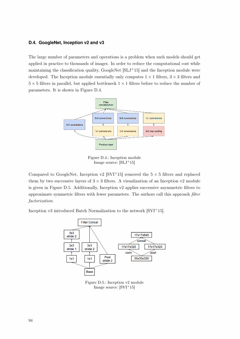
D.4. GoogleNet, Inception v2 and v3

The large number of parameters and operations is a problem when such models should getapplied in practice to thousands of images. In order to reduce the computational cost whilemaintaining the classification quality, GoogleNet [SLJ+15] and the Inception module weredeveloped. The Inception module essentially only computes 1× 1 filters, 3× 3 filters and5× 5 filters in parallel, but applied bottleneck 1× 1 filters before to reduce the number ofparameters. It is shown in Figure D.4.

Figure D.4.: Inception moduleImage source: [SLJ+15]

Compared to GoogleNet, Inception v2 [SVI+15] removed the 5 × 5 filters and replacedthem by two successive layers of 3× 3 filters. A visualization of an Inception v2 moduleis given in Figure D.5. Additionally, Inception v2 applies successive asymmetric filters toapproximate symmetric filters with fewer parameters. The authors call this approach filterfactorization.

Inception v3 introduced Batch Normalization to the network [SVI+15].

Figure D.5.: Inception v2 moduleImage source: [SVI+15]

94

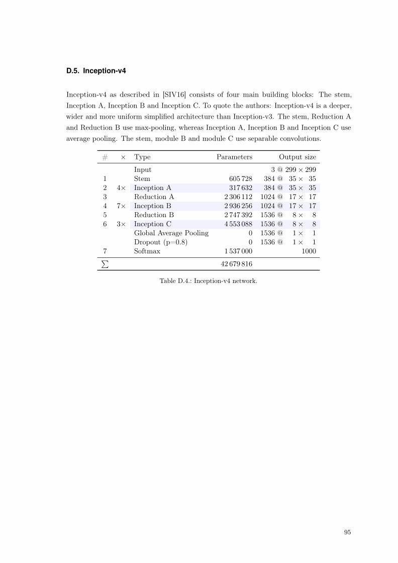
D.5. Inception-v4

Inception-v4 as described in [SIV16] consists of four main building blocks: The stem,Inception A, Inception B and Inception C. To quote the authors: Inception-v4 is a deeper,wider and more uniform simplified architecture than Inception-v3. The stem, Reduction Aand Reduction B use max-pooling, whereas Inception A, Inception B and Inception C useaverage pooling. The stem, module B and module C use separable convolutions.

# × Type Parameters Output size

Input 3 @ 299× 2991 Stem 605 728 384 @ 35× 352 4× Inception A 317 632 384 @ 35× 353 Reduction A 2 306 112 1024 @ 17× 174 7× Inception B 2 936 256 1024 @ 17× 175 Reduction B 2 747 392 1536 @ 8× 86 3× Inception C 4 553 088 1536 @ 8× 8

Global Average Pooling 0 1536 @ 1× 1Dropout (p=0.8) 0 1536 @ 1× 1

7 Softmax 1 537 000 1000∑42 679 816

Table D.4.: Inception-v4 network.

95

E. Datasets

Well-known benchmark datasets for classification problems in computer vision are listedin Table E.1. The best results known to me are given in Table E.2. However, every semanticsegmentation dataset (e.g., PASCAL VOC) can also be used to benchmark image classifiersusing Algorithm 2.

DatabaseImage Resolution(width × height)

Numberof

Images

Numberof

Classes

Channels Data source

MNIST 28 px× 28 px 70 000 10 1 [YL98, LBBH98]HASYv2 32 px× 32 px 168 233 369 1 [Tho17a]

SVHN 32 px× 32 px 630 420 10 3[NWC+11b],[NWC+11a]

CIFAR-10 32 px× 32 px 60 000 10 3 [Kri, KH09]CIFAR-100 32 px× 32 px 60 000 100 3 [Kri, KH09]STL-10 96 px× 96 px 13 000 10 3 [CLN11, CLN10]

Caltech-101 (80 px− 3481 px)×(92 px− 3999 px)

9144 102 3 [FFP03, FFFP06]

Caltech-256 (75 px− 7913 px)×(75 px− 7913 px)

30 607 257 3 [Gri06, GG07]

ILSVRC 20121 (8 px− 9331 px)×(10 px− 6530 px)

1.2 · 106 1000 3 [Ima12, RDS+14]

Places3652 (290px− 3158px)×(225px− 2630px)

1.8 · 106 365 3 [Zho16, ZKL+16]

GTSRB (25 px− 266 px)×(25 px− 232 px)

51 839 43 3 [SSSI, SSSI12]

Asirra3 (4 px− 500 px)×(4 px− 500 px)

25 000 2 3 [Asi17, EDHS07]

Graz-02 480 px× 640 pxand 640 px× 480 px 1096 3 3 [Mar08, MS07]

Table E.1.: An overview over publicly available image databases for classification. The numberof images row gives the sum of the training and the test images. Some datasets, likeSVHN, have additional unlabeled data which is not given in this table.

1ImageNet Large Scale Visual Recognition Competition2The dimensions are only calculated for the validation set.3Asirra is a CAPTCHA created by Microsoft and was used in the “Cats vs Dogs” competition on Kaggle

97

Dataset Model type / name Result ScoreAchieved /Claimed by

MNIST — 0.21 % error [WZZ+13]HASYv2 TF-CNN 81.00 % accuracy [Tho17a]SVHN DenseNet (k = 24) 1.59 % error [HLW16]CIFAR-10 DenseNet-BC (k = 40) 3.46 % error [HLW16]CIFAR-100 WRN-28-10 16.21 % error [LH16]STL-10 SWWAE-4layer 74.80 % accuracy [ZMGL15]Caltech-101 SPP-net (pretrained) 93.42 %±0.5 % accuracy [HZRS14]Caltech-256 ZF-Net (pretrained) 74.2 %±0.3 % accuracy [ZF14]ImageNet 2012 ResNet ensemble 3.57 % Top-5 error [HZRS15a]GTSRB MCDNN 99.46 % accuracy [SL11]Asirra SVM 82.7 % accuracy [Gol08]Graz-02 Optimal NBNN 78.98 % accuracy [BMDP10]

Table E.2.: An overview over state of the art results achieved in computer vision datasets.

Algorithm 2 Create a classification dataset from a semantic segmentation datasetRequire: Semantic segmentation dataset (DS)procedure CreateDataset(Annotated dataset DS)

DC ← List

w ← desired image widthh← desired image heightfor Image and associated label (x, y) in DS do

i← randint(0, L.width− w)

j ← randint(0, L.height− h)

cL ← crop(y, (i, j), (i+ w, j + h))

if at least 50% of s are of one class thencI ← crop(x, (i, j), (i+ w, j + h))

D.append((cI , cL))

return (DC)

98

F. List of Tables

2.1 Pooling types . . . . . . . . . . . . . . . . . . . . . . . . . . . . . . . . . . . 8

5.1 Baseline architecture . . . . . . . . . . . . . . . . . . . . . . . . . . . . . . . 395.2 Baseline model evaluation . . . . . . . . . . . . . . . . . . . . . . . . . . . . 405.3 Baseline model speed comparison . . . . . . . . . . . . . . . . . . . . . . . . 405.4 Clustering errors for spectral clustering and CMO on CIFAR-100 . . . . . . 525.5 Differences in spectral clustering and CMO. . . . . . . . . . . . . . . . . . . 525.6 Accuracies for hierarchy of classifiers on CIFAR-100 . . . . . . . . . . . . . . 535.7 Parameters of models with increased capacity . . . . . . . . . . . . . . . . . 545.8 Training time for models with increased capacity . . . . . . . . . . . . . . . 545.9 Baseline model training time . . . . . . . . . . . . . . . . . . . . . . . . . . 595.10 Activation function properties . . . . . . . . . . . . . . . . . . . . . . . . . . 625.11 Activation function evaluation results on CIFAR-100 . . . . . . . . . . . . . 635.12 Activation function timing results on CIFAR-100 . . . . . . . . . . . . . . . 635.13 Activation function evaluation results on MNIST . . . . . . . . . . . . . . . 645.14 Optimized architecture . . . . . . . . . . . . . . . . . . . . . . . . . . . . . . 665.15 Optimized model evaluation results . . . . . . . . . . . . . . . . . . . . . . . 675.16 Optimized model speed comparison . . . . . . . . . . . . . . . . . . . . . . . 675.17 Optimized model mean training epochs . . . . . . . . . . . . . . . . . . . . . 685.18 Optimized model trained with early stopping vs training with more data . . 695.19 Model regularization with early stopping on training loss . . . . . . . . . . . 695.20 Model regularization with early stopping on training loss - Training time . . 69

A.1 99-percentile intervals for filter weights on CIFAR-100 . . . . . . . . . . . . 75A.2 Activation function evaluation results on HASYv2 . . . . . . . . . . . . . . . 77A.3 Activation function evaluation results on STL-10 . . . . . . . . . . . . . . . 78

B.1 Data augmentation techniques . . . . . . . . . . . . . . . . . . . . . . . . . . 80B.2 Weight initialization schemes . . . . . . . . . . . . . . . . . . . . . . . . . . 81B.3 Activation functions . . . . . . . . . . . . . . . . . . . . . . . . . . . . . . . 84

D.1 LeNet-5 architecture . . . . . . . . . . . . . . . . . . . . . . . . . . . . . . . 90D.2 AlexNet architecture . . . . . . . . . . . . . . . . . . . . . . . . . . . . . . . 91D.3 VGG-16 D architecture . . . . . . . . . . . . . . . . . . . . . . . . . . . . . . 93D.4 Inception-v4 network . . . . . . . . . . . . . . . . . . . . . . . . . . . . . . . 95

99

E.1 Image Benchmark datasets . . . . . . . . . . . . . . . . . . . . . . . . . . . . 97E.2 State of the Art results . . . . . . . . . . . . . . . . . . . . . . . . . . . . . . 98

100

G. List of Figures

2.1 Application of a single image filter (Convolution) . . . . . . . . . . . . . . . 32.2 Application of a convolutional layer . . . . . . . . . . . . . . . . . . . . . . . 62.3 Max pooling . . . . . . . . . . . . . . . . . . . . . . . . . . . . . . . . . . . . 82.4 ResNet module . . . . . . . . . . . . . . . . . . . . . . . . . . . . . . . . . . 112.5 Aggregation block . . . . . . . . . . . . . . . . . . . . . . . . . . . . . . . . 122.6 Dense block . . . . . . . . . . . . . . . . . . . . . . . . . . . . . . . . . . . . 132.7 Validation curve . . . . . . . . . . . . . . . . . . . . . . . . . . . . . . . . . 172.8 Validation curve with plateaus . . . . . . . . . . . . . . . . . . . . . . . . . 182.9 Learning curve . . . . . . . . . . . . . . . . . . . . . . . . . . . . . . . . . . 202.10 Occlusion analysis . . . . . . . . . . . . . . . . . . . . . . . . . . . . . . . . 252.11 Filter visualization . . . . . . . . . . . . . . . . . . . . . . . . . . . . . . . . 26

3.1 Cascade-correlation network . . . . . . . . . . . . . . . . . . . . . . . . . . . 28

4.1 Class Tree . . . . . . . . . . . . . . . . . . . . . . . . . . . . . . . . . . . . . 33

5.1 Baseline architecture . . . . . . . . . . . . . . . . . . . . . . . . . . . . . . . 395.2 Baseline model filter weight distribution . . . . . . . . . . . . . . . . . . . . 425.3 Baseline model bias weight distribution . . . . . . . . . . . . . . . . . . . . . 425.4 Baseline model γ distribution . . . . . . . . . . . . . . . . . . . . . . . . . . 435.5 Baseline model β distribution . . . . . . . . . . . . . . . . . . . . . . . . . . 435.6 Baseline model filter weight range distribution . . . . . . . . . . . . . . . . . 445.7 Baseline model CIFAR-100 validation accuracy . . . . . . . . . . . . . . . . 455.8 Baseline Weight updates (mean) . . . . . . . . . . . . . . . . . . . . . . . . 465.9 Baseline Weight updates (maximum) . . . . . . . . . . . . . . . . . . . . . . 475.10 Baseline Weight updates (sum) . . . . . . . . . . . . . . . . . . . . . . . . . 475.11 Confusion matrices for CIFAR-10 . . . . . . . . . . . . . . . . . . . . . . . . 485.12 Confusion matrices for GTSRB . . . . . . . . . . . . . . . . . . . . . . . . . 495.13 Confusion matrices for HASYv2 . . . . . . . . . . . . . . . . . . . . . . . . . 505.14 Confusion matrix of CIFAR-100 . . . . . . . . . . . . . . . . . . . . . . . . . 515.15 Mean weight updates of model with bottleneck . . . . . . . . . . . . . . . . 555.16 Optimized architecture . . . . . . . . . . . . . . . . . . . . . . . . . . . . . . 67

A.1 Image Filters . . . . . . . . . . . . . . . . . . . . . . . . . . . . . . . . . . . 75A.2 Bias weight distribution without BN . . . . . . . . . . . . . . . . . . . . . . 76

101

A.3 Maximum weight updates of baseline with bottleneck . . . . . . . . . . . . . 77A.4 Sum of weight updates of baseline with bottleneck . . . . . . . . . . . . . . 78

B.1 Activation functions . . . . . . . . . . . . . . . . . . . . . . . . . . . . . . . 85

D.1 LeNet-5 architecture . . . . . . . . . . . . . . . . . . . . . . . . . . . . . . . 90D.2 AlexNet architecture . . . . . . . . . . . . . . . . . . . . . . . . . . . . . . . 91D.3 VGG-16 D architecture . . . . . . . . . . . . . . . . . . . . . . . . . . . . . . 92D.4 Inception module . . . . . . . . . . . . . . . . . . . . . . . . . . . . . . . . . 94D.5 Inception v2 module . . . . . . . . . . . . . . . . . . . . . . . . . . . . . . . 94

102

H. Bibliography

[AAB+16] M. Abadi, A. Agarwal et al., “Tensorflow: Large-scale machine learning onheterogeneous distributed systems,” arXiv preprint arXiv:1603.04467, Mar.2016. [Online]. Available: https://arxiv.org/abs/1603.04467

[ABKS99] M. Ankerst, M. M. Breunig et al., “OPTICS: Ordering points to identify theclustering structure,” in ACM Sigmod record, vol. 28, no. 2. ACM, 1999, pp.49–60.

[ADG+16] M. Andrychowicz, M. Denil et al., “Learning to learn by gradient descent bygradient descent,” in Advances in Neural Information Processing Systems 29(NIPS), D. D. Lee, M. Sugiyama et al., Eds. Curran Associates, Inc., Mar.2016, pp. 3981–3989. [Online]. Available: http://papers.nips.cc/paper/6461-learning-to-learn-by-gradient-descent-by-gradient-descent.pdf

[AM15] M. T. Alexander Mordvintsev, Christopher Olah, “Inceptionism:Going deeper into neural networks,” Jun. 2015. [Online]. Avail-able: https://research.googleblog.com/2015/06/inceptionism-going-deeper-into-neural.html

[Asi17] “Kaggle cats and dogs dataset,” Oct. 2017. [Online]. Available: https://www.microsoft.com/en-us/download/details.aspx?id=54765

[BB12] J. Bergstra and Y. Bengio, “Random search for hyper-parameter optimization,”Journal of Machine Learning Research, vol. 13, no. Feb, pp. 281–305,Feb. 2012. [Online]. Available: http://jmlr.csail.mit.edu/papers/volume13/bergstra12a/bergstra12a.pdf

[BCW+17] J. Bao, D. Chen et al., “CVAE-GAN: Fine-grained image generation throughasymmetric training,” arXiv preprint arXiv:1703.10155, Mar. 2017. [Online].Available: https://arxiv.org/abs/1703.10155

[BDLB09] J. Bergstra, G. Desjardins et al., “Quadratic polynomials learn better im-age features,” Département d’Informatique et de Recherche Opérationnelle,Université de Montréal, Tech. Rep. 1337, 2009.

[BGNR16] B. Baker, O. Gupta et al., “Designing neural network architectures usingreinforcement learning,” arXiv preprint arXiv:1611.02167, Nov. 2016. [Online].Available: https://arxiv.org/abs/1611.02167

103

https://arxiv.org/abs/1603.04467

http://papers.nips.cc/paper/6461-learning-to-learn-by-gradient-descent-by-gradient-descent.pdf

http://papers.nips.cc/paper/6461-learning-to-learn-by-gradient-descent-by-gradient-descent.pdf

https://research.googleblog.com/2015/06/inceptionism-going-deeper-into-neural.html

https://research.googleblog.com/2015/06/inceptionism-going-deeper-into-neural.html

https://www.microsoft.com/en-us/download/details.aspx?id=54765

https://www.microsoft.com/en-us/download/details.aspx?id=54765

http://jmlr.csail.mit.edu/papers/volume13/bergstra12a/bergstra12a.pdf

http://jmlr.csail.mit.edu/papers/volume13/bergstra12a/bergstra12a.pdf



[BM93] U. Bodenhausen and S. Manke, Automatically Structured NeuralNetworks For Handwritten Character And Word Recognition. London:Springer London, Sep. 1993, pp. 956–961. [Online]. Available: http://dx.doi.org/10.1007/978-1-4471-2063-6_283

[BMDP10] R. Behmo, P. Marcombes et al., “Towards optimal naive Bayes nearestneighbor,” in European Conference on Computer Vision (ECCV). Springer,2010, pp. 171–184.

[BPL10] Y.-L. Boureau, J. Ponce, and Y. LeCun, “A theoretical analysis offeature pooling in visual recognition,” in International Conference onMachine Learning (ICML), no. 27, 2010, pp. 111–118. [Online]. Available:http://yann.lecun.com/exdb/publis/pdf/boureau-icml-10.pdf

[BSF94] Y. Bengio, P. Simard, and P. Frasconi, “Learning long-term dependencieswith gradient descent is difficult,” IEEE transactions on neural networks,vol. 5, no. 2, pp. 157–166, 1994.

[Cha92] C. Charalambous, “Conjugate gradient algorithm for efficient trainingof artificial neural networks,” IEEE Proceedings G-Circuits, Devicesand Systems, vol. 139, no. 3, pp. 301–310, 1992. [Online]. Available:http://ieeexplore.ieee.org/document/143326/

[Cho15] F. Chollet, “Keras,” https://github.com/fchollet/keras, 2015.

[CLN10] A. Coates, H. Lee, and A. Y. Ng, “An analysis of single-layer networksin unsupervised feature learning,” Ann Arbor, vol. 1001, no. 48109,p. 2, 2010. [Online]. Available: http://cs.stanford.edu/~acoates/papers/coatesleeng_aistats_2011.pdf

[CLN11] A. Coates, H. Lee, and A. Y. Ng, “STL-10 dataset,” 2011. [Online]. Available:http://cs.stanford.edu/~acoates/stl10

[CMS12] D. Ciregan, U. Meier, and J. Schmidhuber, “Multi-column deep neuralnetworks for image classification,” in Conference on Computer Vision andPattern Recognition (CVPR). IEEE, Feb. 2012, pp. 3642–3649. [Online].Available: https://arxiv.org/abs/1202.2745v1

[CUH15] D.-A. Clevert, T. Unterthiner, and S. Hochreiter, “Fast and accuratedeep network learning by exponential linear units (ELUs),” arXivpreprint arXiv:1511.07289, Nov. 2015. [Online]. Available: https://arxiv.org/abs/1511.07289

[CWV+14] S. Chetlur, C. Woolley et al., “cuDNN: Efficient primitives for deeplearning,” arXiv preprint arXiv:1410.0759, Oct. 2014. [Online]. Available:https://arxiv.org/abs/1410.0759

104

http://dx.doi.org/10.1007/978-1-4471-2063-6_283

http://dx.doi.org/10.1007/978-1-4471-2063-6_283

http://yann.lecun.com/exdb/publis/pdf/boureau-icml-10.pdf

http://ieeexplore.ieee.org/document/143326/

https://github.com/fchollet/keras

http://cs.stanford.edu/~acoates/papers/coatesleeng_aistats_2011.pdf

http://cs.stanford.edu/~acoates/papers/coatesleeng_aistats_2011.pdf

http://cs.stanford.edu/~acoates/stl10

https://arxiv.org/abs/1202.2745v1




[DBB+01] C. Dugas, Y. Bengio et al., “Incorporating second-order functionalknowledge for better option pricing,” in Advances in Neural Infor-mation Processing Systems 13 (NIPS), T. K. Leen, T. G. Dietterich,and V. Tresp, Eds. MIT Press, 2001, pp. 472–478. [Online].Available: http://papers.nips.cc/paper/1920-incorporating-second-order-functional-knowledge-for-better-option-pricing.pdf

[DDFK16] S. Dieleman, J. De Fauw, and K. Kavukcuoglu, “Exploiting cyclic symmetryin convolutional neural networks,” arXiv preprint arXiv:1602.02660, Feb.2016. [Online]. Available: https://arxiv.org/abs/1602.02660

[DHS11] J. Duchi, E. Hazan, and Y. Singer, “Adaptive subgradient methods foronline learning and stochastic optimization,” Journal of Machine LearningResearch, vol. 12, no. Jul, pp. 2121–2159, 2011. [Online]. Available:http://www.jmlr.org/papers/volume12/duchi11a/duchi11a.pdf

[DHS16] J. Dai, K. He, and J. Sun, “Instance-aware semantic segmentation viamulti-task network cascades,” in Conference on Computer Vision and PatternRecognition (CVPR). IEEE, 2016, pp. 3150–3158. [Online]. Available:https://arxiv.org/abs/1512.04412

[DJ99] W. Duch and N. Jankowski, “Survey of neural transfer functions,” NeuralComputing Surveys, vol. 2, no. 1, pp. 163–212, 1999. [Online]. Available:ftp://ftp.icsi.berkeley.edu/pub/ai/jagota/vol2_6.pdf

[Doz15] T. Dozat, “Incorporating Nesterov momentum into Adam,” StanfordUniversity, Tech. Rep., 2015. [Online]. Available: http://cs229.stanford.edu/proj2015/054_report.pdf

[DSRB14] A. Dosovitskiy, J. T. Springenberg et al., “Discriminative unsupervisedfeature learning with convolutional neural networks,” in Advances in NeuralInformation Processing Systems 27 (NIPS), Z. Ghahramani, M. Wellinget al., Eds. Curran Associates, Inc., 2014, pp. 766–774. [Online].Available: http://papers.nips.cc/paper/5548-discriminative-unsupervised-feature-learning-with-convolutional-neural-networks.pdf

[DWD15] S. Dieleman, K. W. Willett, and J. Dambre, “Rotation-invariant convolutionalneural networks for galaxy morphology prediction,” Monthly notices of theroyal astronomical society, vol. 450, no. 2, pp. 1441–1459, 2015.

[EDHS07] J. Elson, J. J. Douceur et al., “Asirra: A CAPTCHA thatexploits interest-aligned manual image categorization,” in ACM Con-ference on Computer and Communications Security (CCS), no. 14.Association for Computing Machinery, Inc., Oct. 2007. [Online].

105

http://papers.nips.cc/paper/1920-incorporating-second-order-functional-knowledge-for-better-option-pricing.pdf

http://papers.nips.cc/paper/1920-incorporating-second-order-functional-knowledge-for-better-option-pricing.pdf


http://www.jmlr.org/papers/volume12/duchi11a/duchi11a.pdf


ftp://ftp.icsi.berkeley.edu/pub/ai/jagota/vol2_6.pdf

http://cs229.stanford.edu/proj2015/054_report.pdf

http://cs229.stanford.edu/proj2015/054_report.pdf

http://papers.nips.cc/paper/5548-discriminative-unsupervised-feature-learning-with-convolutional-neural-networks.pdf

http://papers.nips.cc/paper/5548-discriminative-unsupervised-feature-learning-with-convolutional-neural-networks.pdf

Available: https://www.microsoft.com/en-us/research/publication/asirra-a-captcha-that-exploits-interest-aligned-manual-image-categorization/

[EKS+96] M. Ester, H.-P. Kriegel et al., “A density-based algorithm for discoveringclusters in large spatial databases with noise.” in Kdd, vol. 96, no. 34, 1996,pp. 226–231.

[ES03] A. E. Eiben and J. E. Smith, Introduction to evolutionary computing.Springer, 2003, vol. 53. [Online]. Available: https://dx.doi.org/10.1007/978-3-662-44874-8

[Fah88] S. E. Fahlman, “An empirical study of learning speed in back-propagationnetworks,” 1988. [Online]. Available: http://repository.cmu.edu/cgi/viewcontent.cgi?article=2799&context=compsci

[FFFP06] L. Fei-Fei, R. Fergus, and P. Perona, “One-shot learning of objectcategories,” IEEE transactions on pattern analysis and machine intelligence,vol. 28, no. 4, pp. 594–611, Apr. 2006. [Online]. Available: http://vision.stanford.edu/documents/Fei-FeiFergusPerona2006.pdf

[FFP03] R. F. Fei-Fei and P. Perona, “Caltech 101,” 2003. [Online]. Available: http://www.vision.caltech.edu/Image_Datasets/Caltech101/Caltech101.html

[FGMR10] P. F. Felzenszwalb, R. B. Girshick et al., “Object detection with discrimina-tively trained part-based models,” IEEE transactions on pattern analysis andmachine intelligence, vol. 32, no. 9, pp. 1627–1645, 2010.

[FL89] S. E. Fahlman and C. Lebiere, “The cascade-correlation learning architecture,”1989. [Online]. Available: http://repository.cmu.edu/compsci/1938/

[GB10] X. Glorot and Y. Bengio, “Understanding the difficulty of training deepfeedforward neural networks.” in Aistats, vol. 9, 2010, pp. 249–256. [Online].Available: http://jmlr.org/proceedings/papers/v9/glorot10a/glorot10a.pdf

[GBB11] X. Glorot, A. Bordes, and Y. Bengio, “Deep sparse rectifier neuralnetworks.” in Aistats, vol. 15, no. 106, 2011, p. 275. [Online]. Available:http://www.jmlr.org/proceedings/papers/v15/glorot11a/glorot11a.pdf

[GDDM14] R. Girshick, J. Donahue et al., “Rich feature hierarchies for accurate objectdetection and semantic segmentation,” in Conference on Computer Visionand Pattern Recognition (CVPR). IEEE, 2014, pp. 580–587. [Online].Available: https://arxiv.org/abs/1311.2524

[GG07] P. P. Greg Griffin, Alex Holub, “Caltech-256 object category dataset,” Apr.2007. [Online]. Available: http://authors.library.caltech.edu/7694/

106

https://www.microsoft.com/en-us/research/publication/asirra-a-captcha-that-exploits-interest-aligned-manual-image-categorization/

https://www.microsoft.com/en-us/research/publication/asirra-a-captcha-that-exploits-interest-aligned-manual-image-categorization/

https://dx.doi.org/10.1007/978-3-662-44874-8

https://dx.doi.org/10.1007/978-3-662-44874-8

http://repository.cmu.edu/cgi/viewcontent.cgi?article=2799&context=compsci

http://repository.cmu.edu/cgi/viewcontent.cgi?article=2799&context=compsci

http://vision.stanford.edu/documents/Fei-FeiFergusPerona2006.pdf

http://vision.stanford.edu/documents/Fei-FeiFergusPerona2006.pdf

http://www.vision.caltech.edu/Image_Datasets/Caltech101/Caltech101.html

http://www.vision.caltech.edu/Image_Datasets/Caltech101/Caltech101.html

http://repository.cmu.edu/compsci/1938/

http://jmlr.org/proceedings/papers/v9/glorot10a/glorot10a.pdf

http://www.jmlr.org/proceedings/papers/v15/glorot11a/glorot11a.pdf


http://authors.library.caltech.edu/7694/

[GG16] Y. Gal and Z. Ghahramani, “Bayesian convolutional neural networks withBernoulli approximate variational inference,” arXiv preprint arXiv:1506.02158,Jan. 2016. [Online]. Available: https://arxiv.org/abs/1506.02158v6

[GJ02] M. R. Garey and D. S. Johnson, Computers and intractability. wh freemanNew York, 2002, vol. 29.

[GJS76] M. R. Garey, D. S. Johnson, and L. Stockmeyer, “Some simplified NP-completegraph problems,” Theoretical computer science, vol. 1, no. 3, pp. 237–267,1976.

[Gol08] P. Golle, “Machine learning attacks against the Asirra CAPTCHA,” in ACMconference on Computer and communications security (CCS), no. 15. ACM,2008, pp. 535–542.

[Gra15] B. Graham, “Fractional max-pooling,” arXiv preprint arXiv:1412.6071, May2015. [Online]. Available: https://arxiv.org/abs/1412.6071

[Gri06] A. P. Griffin, G. Holub, “Caltech 256,” 2006. [Online]. Available:http://www.vision.caltech.edu/Image_Datasets/Caltech256/

[GWFM+13] I. J. Goodfellow, D. Warde-Farley et al., “Maxout networks.” ICML,vol. 28, no. 3, pp. 1319–1327, 2013. [Online]. Available: http://www.jmlr.org/proceedings/papers/v28/goodfellow13.pdf

[HAE16] M. Huh, P. Agrawal, and A. A. Efros, “What makes ImageNet good fortransfer learning?” arXiv preprint arXiv:1608.08614, Aug. 2016. [Online].Available: https://arxiv.org/abs/1608.08614

[Han89] S. J. Hanson, “Meiosis networks.” in NIPS, 1989, pp. 533–541. [Online].Available: http://papers.nips.cc/paper/227-meiosis-networks.pdf

[Har15] M. Harris, “New features in CUDA 7.5,” Jul. 2015. [Online]. Available:https://devblogs.nvidia.com/parallelforall/new-features-cuda-7-5/

[HLW16] G. Huang, Z. Liu, and K. Q. Weinberger, “Densely connected convolutionalnetworks,” arXiv preprint arXiv:1608.06993, Aug. 2016. [Online]. Available:https://arxiv.org/abs/1608.06993v1

[HM16] M. Hardt and T. Ma, “Identity matters in deep learning,” arXivpreprint arXiv:1611.04231, Nov. 2016. [Online]. Available: https://arxiv.org/abs/1611.04231

[How13] A. G. Howard, “Some improvements on deep convolutional neural networkbased image classification,” arXiv preprint arXiv:1312.5402, Dec. 2013.[Online]. Available: https://arxiv.org/abs/1312.5402

107



http://www.vision.caltech.edu/Image_Datasets/Caltech256/

http://www.jmlr.org/proceedings/papers/v28/goodfellow13.pdf

http://www.jmlr.org/proceedings/papers/v28/goodfellow13.pdf


http://papers.nips.cc/paper/227-meiosis-networks.pdf

https://devblogs.nvidia.com/parallelforall/new-features-cuda-7-5/





[HPK11] J. Han, J. Pei, and M. Kamber, Data mining: concepts and techniques.Elsevier, 2011.

[HPN+16] S. Han, J. Pool et al., “DSD: Regularizing deep neural networks withdense-sparse-dense training flow,” arXiv preprint arXiv:1607.04381, Jul. 2016.[Online]. Available: https://arxiv.org/abs/1607.04381

[HPTD15] S. Han, J. Pool et al., “Learning both weights and connections for efficientneural network,” in Advances in Neural Information Processing Systems 28(NIPS), C. Cortes, N. D. Lawrence et al., Eds. Curran Associates, Inc., Jun.2015, pp. 1135–1143. [Online]. Available: http://papers.nips.cc/paper/5784-learning-both-weights-and-connections-for-efficient-neural-network.pdf

[HSK+12] G. E. Hinton, N. Srivastava et al., “Improving neural networks by preventingco-adaptation of feature detectors,” arXiv preprint arXiv:1207.0580, Jul.2012. [Online]. Available: https://arxiv.org/abs/1207.0580

[HSL+16] G. Huang, Y. Sun et al., “Deep networks with stochastic depth,”arXiv preprint arXiv:1603.09382, Mar. 2016. [Online]. Available: https://arxiv.org/abs/1603.09382

[HSW93] B. Hassibi, D. G. Stork, and G. J. Wolff, “Optimal brain surgeonand general network pruning,” in International Conference on NeuralNetworks. IEEE, 1993, pp. 293–299. [Online]. Available: http://ee.caltech.edu/Babak/pubs/conferences/00298572.pdf

[HVD15] G. Hinton, O. Vinyals, and J. Dean, “Distilling the knowledge in a neuralnetwork,” arXiv preprint arXiv:1503.02531, Mar. 2015. [Online]. Available:https://arxiv.org/abs/1503.02531

[HZRS14] K. He, X. Zhang et al., “Spatial pyramid pooling in deep convolutionalnetworks for visual recognition,” in European Conference on ComputerVision (ECCV). Springer, 2014, pp. 346–361. [Online]. Available:https://arxiv.org/abs/1406.4729

[HZRS15a] K. He, X. Zhang et al., “Deep residual learning for image recognition,”arXiv preprint arXiv:1512.03385, Dec. 2015. [Online]. Available: https://arxiv.org/abs/1512.03385v1

[HZRS15b] K. He, X. Zhang et al., “Delving deep into rectifiers: Surpassing human-levelperformance on imagenet classification,” in International Conference onComputer Vision (ICCV), Feb. 2015, pp. 1026–1034. [Online]. Available:https://arxiv.org/abs/1502.01852

[Ima12] “Imagenet large scale visual recognition challenge 2012 (ILSVRC2012),”

108


http://papers.nips.cc/paper/5784-learning-both-weights-and-connections-for-efficient-neural-network.pdf

http://papers.nips.cc/paper/5784-learning-both-weights-and-connections-for-efficient-neural-network.pdf




http://ee.caltech.edu/Babak/pubs/conferences/00298572.pdf

http://ee.caltech.edu/Babak/pubs/conferences/00298572.pdf






2012. [Online]. Available: http://www.image-net.org/challenges/LSVRC/2012/nonpub-downloads

[IS15] S. Ioffe and C. Szegedy, “Batch normalization: Accelerating deep networktraining by reducing internal covariate shift,” arXiv preprint arXiv:1502.03167,Feb. 2015. [Online]. Available: https://arxiv.org/abs/1502.03167

[JXF+16] X. Jin, C. Xu et al., “Deep learning with s-shaped rectified linear activationunits,” in Thirtieth AAAI Conference on Artificial Intelligence, Dec. 2016.[Online]. Available: https://arxiv.org/abs/1512.07030

[Kar11] A. Karpathy, “Lessons learned from manually classifying CIFAR-10,” Apr.2011. [Online]. Available: http://karpathy.github.io/2011/04/27/manually-classifying-cifar10/

[KB14] D. Kingma and J. Ba, “Adam: A method for stochastic optimization,”arXiv preprint arXiv:1412.6980, Dec. 2014. [Online]. Available: https://arxiv.org/abs/1412.6980

[KH09] A. Krizhevsky and G. Hinton, “Learning multiple layers of features from tinyimages,” Apr. 2009. [Online]. Available: https://www.cs.toronto.edu/~kriz/learning-features-2009-TR.pdf

[KMN+16] N. S. Keskar, D. Mudigere et al., “On large-batch training for deep learning:Generalization gap and sharp minima,” arXiv preprint arXiv:1609.04836,Sep. 2016. [Online]. Available: https://arxiv.org/abs/1609.04836

[Koc15] T. Kocmánek, “HyperNEAT and novelty search for image recognition,” Ph.D.dissertation, Master’s thesis, Czech Technical University in Prague, 2015.[Online]. Available: http://kocmi.tk/photos/DiplomaThesis.pdf

[KPY+15] Y.-D. Kim, E. Park et al., “Compression of deep convolutional neural networksfor fast and low power mobile applications,” arXiv preprint arXiv:1511.06530,Nov. 2015. [Online]. Available: https://arxiv.org/abs/1511.06530

[KR09] L. Kaufman and P. J. Rousseeuw, Finding groups in data: an introduction tocluster analysis. John Wiley & Sons, 2009, vol. 344.

[Kri] A. Krizhevsky, “The CIFAR-10 dataset.” [Online]. Available: https://www.cs.toronto.edu/~kriz/cifar.html

[KS02] V. Kurkova and M. Sanguineti, “Comparison of worst case errors in linearand neural network approximation,” IEEE Transactions on InformationTheory, vol. 48, no. 1, pp. 264–275, Jan. 2002. [Online]. Available:http://ieeexplore.ieee.org/abstract/document/971754/

109

http://www.image-net.org/challenges/LSVRC/2012/nonpub-downloads

http://www.image-net.org/challenges/LSVRC/2012/nonpub-downloads



http://karpathy.github.io/2011/04/27/manually-classifying-cifar10/

http://karpathy.github.io/2011/04/27/manually-classifying-cifar10/



https://www.cs.toronto.edu/~kriz/learning-features-2009-TR.pdf

https://www.cs.toronto.edu/~kriz/learning-features-2009-TR.pdf


http://kocmi.tk/photos/DiplomaThesis.pdf


https://www.cs.toronto.edu/~kriz/cifar.html

https://www.cs.toronto.edu/~kriz/cifar.html

http://ieeexplore.ieee.org/abstract/document/971754/

[KSH12] A. Krizhevsky, I. Sutskever, and G. E. Hinton, “Imagenet classificationwith deep convolutional neural networks,” in Advances in NeuralInformation Processing Systems 25 (NIPS), F. Pereira, C. J. C. Burgeset al., Eds. Curran Associates, Inc., 2012, pp. 1097–1105. [Online].Available: http://papers.nips.cc/paper/4824-imagenet-classification-with-deep-convolutional-neural-networks.pdf

[KSlB+10] K. Kavukcuoglu, P. Sermanet et al., “Learning convolutional featurehierarchies for visual recognition,” in Advances in Neural InformationProcessing Systems 23 (NIPS), J. D. Lafferty, C. K. I. Williamset al., Eds. Curran Associates, Inc., 2010, pp. 1090–1098. [Online].Available: http://papers.nips.cc/paper/4133-learning-convolutional-feature-hierarchies-for-visual-recognition.pdf

[LAE+16] W. Liu, D. Anguelov et al., “SSD: Single shot multibox detector,” inEuropean Conference on Computer Vision (ECCV). Springer, 2016, pp.21–37. [Online]. Available: https://arxiv.org/abs/1512.02325

[Las17] “Noise layers,” Jan. 2017. [Online]. Available: http://lasagne.readthedocs.io/en/latest/modules/layers/noise.html#lasagne.layers.DropoutLayer

[LBBH98] Y. LeCun, L. Bottou et al., “Gradient-based learning applied to documentrecognition,” Proceedings of the IEEE, vol. 86, no. 11, pp. 2278–2324, Nov.1998. [Online]. Available: http://yann.lecun.com/exdb/publis/pdf/lecun-01a.pdf

[LBH15] Y. LeCun, Y. Bengio, and G. Hinton, “Deep learning,” Nature,vol. 521, no. 7553, pp. 436–444, May 2015. [Online]. Available:http://www.nature.com/nature/journal/v521/n7553/abs/nature14539.html

[LBOM98] Y. A. LeCun, L. Bottou et al., Efficient BackProp, ser. Lecture Notes inComputer Science. Berlin, Heidelberg: Springer Berlin Heidelberg, 1998, vol.1524, pp. 9–50. [Online]. Available: http://dx.doi.org/10.1007/3-540-49430-8

[LDS+89] Y. LeCun, J. S. Denker et al., “Optimal brain damage.” in NIPs, vol. 2, 1989,pp. 598–605. [Online]. Available: http://yann.lecun.com/exdb/publis/pdf/lecun-90b.pdf

[Le13] Q. V. Le, “Building high-level features using large scale unsupervisedlearning,” in International conference on acoustics, speech and signalprocessing. IEEE, 2013, pp. 8595–8598. [Online]. Available: http://ieeexplore.ieee.org/stamp/stamp.jsp?arnumber=6639343

[LG16] A. Lavin and S. Gray, “Fast algorithms for convolutional neural networks,” in

110

http://papers.nips.cc/paper/4824-imagenet-classification-with-deep-convolutional-neural-networks.pdf

http://papers.nips.cc/paper/4824-imagenet-classification-with-deep-convolutional-neural-networks.pdf

http://papers.nips.cc/paper/4133-learning-convolutional-feature-hierarchies-for-visual-recognition.pdf

http://papers.nips.cc/paper/4133-learning-convolutional-feature-hierarchies-for-visual-recognition.pdf


http://lasagne.readthedocs.io/en/latest/modules/layers/noise.html#lasagne.layers.DropoutLayer

http://lasagne.readthedocs.io/en/latest/modules/layers/noise.html#lasagne.layers.DropoutLayer

http://yann.lecun.com/exdb/publis/pdf/lecun-01a.pdf

http://yann.lecun.com/exdb/publis/pdf/lecun-01a.pdf

http://www.nature.com/nature/journal/v521/n7553/abs/nature14539.html

http://dx.doi.org/10.1007/3-540-49430-8

http://yann.lecun.com/exdb/publis/pdf/lecun-90b.pdf

http://yann.lecun.com/exdb/publis/pdf/lecun-90b.pdf

http://ieeexplore.ieee.org/stamp/stamp.jsp?arnumber=6639343

http://ieeexplore.ieee.org/stamp/stamp.jsp?arnumber=6639343

Conference on Computer Vision and Pattern Recognition (CVPR). IEEE, Sep.2016, pp. 4013–4021. [Online]. Available: https://arxiv.org/abs/1509.09308

[LGT16] C.-Y. Lee, P. W. Gallagher, and Z. Tu, “Generalizing pooling functions inconvolutional neural networks: Mixed, gated, and tree,” in InternationalConference on Artificial Intelligence and Statistics, 2016. [Online]. Available:https://arxiv.org/abs/1509.08985v2

[LH16] I. Loshchilov and F. Hutter, “SGDR: stochastic gradient descentwith warm restarts,” Learning, Aug. 2016. [Online]. Available: https://arxiv.org/abs/1608.03983

[LJD+16] L. Li, K. Jamieson et al., “Hyperband: A novel bandit-based approach tohyperparameter optimization,” arXiv preprint arXiv:1603.06560, Mar. 2016.[Online]. Available: https://arxiv.org/abs/1603.06560

[LM16] K. Li and J. Malik, “Learning to optimize,” arXiv preprint arXiv:1606.01885,Jun. 2016. [Online]. Available: https://arxiv.org/abs/1606.01885

[LSD15] J. Long, E. Shelhamer, and T. Darrell, “Fully convolutional networks forsemantic segmentation,” in Conference on Computer Vision and PatternRecognition (CVPR). IEEE, Mar. 2015, pp. 3431–3440. [Online]. Available:https://arxiv.org/abs/1411.4038v2

[LX17] A. Y. Lingxi Xie, “Genetic CNN,” arXiv preprint arXiv:1703.01513, Mar.2017. [Online]. Available: https://arxiv.org/abs/1703.01513

[Maj17] S. Majumdar, “Densenet,” GitHub, Feb. 2017. [Online]. Available:https://github.com/titu1994/DenseNet

[Mar08] M. Marszałek, “INRIA annotations for Graz-02 (IG02),” Oct. 2008. [Online].Available: http://lear.inrialpes.fr/people/marszalek/data/ig02/

[MDA15] D. Maclaurin, D. Duvenaud, and R. Adams, “Gradient-based hyperparameteroptimization through reversible learning,” in International Conference onMachine Learning (ICML), 2015, pp. 2113–2122.

[MH08] L. v. d. Maaten and G. Hinton, “Visualizing data using t-SNE,” Journal ofMachine Learning Research, vol. 9, no. Nov, pp. 2579–2605, 2008.

[MHN13] A. L. Maas, A. Y. Hannun, and A. Y. Ng, “Rectifier nonlinearitiesimprove neural network acoustic models,” in Proc. ICML, vol. 30,no. 1, 2013. [Online]. Available: https://web.stanford.edu/~awni/papers/relu_hybrid_icml2013_final.pdf

[MM15] D. Mishkin and J. Matas, “All you need is a good init,” arXiv

111









https://github.com/titu1994/DenseNet

http://lear.inrialpes.fr/people/marszalek/data/ig02/

https://web.stanford.edu/~awni/papers/relu_hybrid_icml2013_final.pdf

https://web.stanford.edu/~awni/papers/relu_hybrid_icml2013_final.pdf

preprint arXiv:1511.06422, Nov. 2015. [Online]. Available: https://arxiv.org/abs/1511.06422

[MP43] W. S. McCulloch and W. Pitts, “A logical calculus of the ideas immanent innervous activity,” The bulletin of mathematical biophysics, vol. 5, no. 4, pp.115–133, 1943.

[MRM15] N. McLaughlin, J. M. D. Rincon, and P. Miller, “Data-augmentation forreducing dataset bias in person re-identification,” in International Conferenceon Advanced Video and Signal Based Surveillance (AVSS), no. 12, Aug. 2015,pp. 1–6. [Online]. Available: http://ieeexplore.ieee.org/abstract/document/7301739/

[MS07] M. Marszalek and C. Schmid, “Accurate object localization withshape masks,” in Conference on Computer Vision and PatternRecognition (CVPR). IEEE, 2007, pp. 1–8. [Online]. Available: http://ieeexplore.ieee.org/document/4270110/

[MSM16] D. Mishkin, N. Sergievskiy, and J. Matas, “Systematic evaluation of CNNadvances on the ImageNet,” arXiv preprint arXiv:1606.02228, Jun. 2016.[Online]. Available: https://arxiv.org/abs/1606.02228

[MV16] A. Mahendran and A. Vedaldi, “Visualizing deep convolutional neuralnetworks using natural pre-images,” International Journal of Computer Vision,pp. 1–23, Apr. 2016. [Online]. Available: https://arxiv.org/abs/1512.02017

[NDRT13] N. Natarajan, I. S. Dhillon et al., “Learning with noisy labels,” in Advancesin Neural Information Processing Systems 26 (NIPS), C. J. C. Burges,L. Bottou et al., Eds. Curran Associates, Inc., 2013, pp. 1196–1204. [Online].Available: http://papers.nips.cc/paper/5073-learning-with-noisy-labels.pdf

[Nes83] Y. Nesterov, “A method of solving a convex programming problem withconvergence rate o (1/k2),” in Soviet Mathematics Doklady, vol. 27, no. 2,1983, pp. 372–376.

[new00] “The training performed by qnstrn,” Aug. 2000. [Online]. Available:http://www1.icsi.berkeley.edu/Speech/faq/nn-train.html

[Ng16] A. Ng, “Nuts and bolts of building ai applications using deep learning,” NIPSTalk, Dec. 2016.

[NH92] S. J. Nowlan and G. E. Hinton, “Simplifying neural networks by softweight-sharing,” Neural computation, vol. 4, no. 4, pp. 473–493, 1992.[Online]. Available: https://www.cs.toronto.edu/~hinton/absps/sunspots.pdf

[NH02] R. T. Ng and J. Han, “CLARANS: A method for clustering objects for spatial

112









http://papers.nips.cc/paper/5073-learning-with-noisy-labels.pdf

http://www1.icsi.berkeley.edu/Speech/faq/nn-train.html

https://www.cs.toronto.edu/~hinton/absps/sunspots.pdf

data mining,” IEEE transactions on knowledge and data engineering, vol. 14,no. 5, pp. 1003–1016, 2002.

[NWC+11a] Y. Netzer, T. Wang et al., “Reading digits in natural images withunsupervised feature learning,” in NIPS workshop on deep learning andunsupervised feature learning, vol. 2011, no. 2, 2011, p. 5. [Online]. Available:http://ufldl.stanford.edu/housenumbers/nips2011_housenumbers.pdf

[NWC+11b] Y. Netzer, T. Wang et al., “The street view house numbers (SVHN) dataset,”2011. [Online]. Available: http://ufldl.stanford.edu/housenumbers/

[NYC16] A. Nguyen, J. Yosinski, and J. Clune, “Multifaceted feature visualization:Uncovering the different types of features learned by each neuron in deepneural networks,” arXiv preprint arXiv:1602.03616, May 2016. [Online].Available: https://arxiv.org/abs/1602.03616

[OHIL16] J. Ortigosa-Hernández, I. Inza, and J. A. Lozano, “Towards competitiveclassifiers for unbalanced classification problems: A study on the performancescores,” arXiv preprint arXiv:1608.08984, Aug. 2016. [Online]. Available:https://arxiv.org/abs/1608.08984

[PMW+15] N. Papernot, P. McDaniel et al., “Distillation as a defense to adversarialperturbations against deep neural networks,” arXiv preprint arXiv:1511.04508,Nov. 2015. [Online]. Available: https://arxiv.org/abs/1511.04508

[Pre98] L. Prechelt, Early Stopping - But When? Berlin, Heidelberg: SpringerBerlin Heidelberg, 1998, pp. 55–69. [Online]. Available: http://dx.doi.org/10.1007/3-540-49430-8_3

[RDS+14] O. Russakovsky, J. Deng et al., “Imagenet large scale visual recognitionchallenge,” arXiv preprint arXiv:1409.0575, vol. 115, no. 3, pp. 211–252, Sep.2014. [Online]. Available: https://arxiv.org/abs/1409.0575

[RFB15] O. Ronneberger, P. Fischer, and T. Brox, “U-net: Convolutional networksfor biomedical image segmentation,” in International Conference on MedicalImage Computing and Computer-Assisted Intervention. Springer, 2015, pp.234–241. [Online]. Available: https://arxiv.org/abs/1505.04597

[RLS10] S. Risi, J. Lehman, and K. O. Stanley, “Evolving the placement and den-sity of neurons in the hyperneat substrate,” in Conference on Genetic andevolutionary computation, no. 12. ACM, 2010, pp. 563–570.

[RSG16] M. T. Ribeiro, S. Singh, and C. Guestrin, “"why should i trust you?":Explaining the predictions of any classifier,” arXiv preprint arXiv:1602.04938,Feb. 2016. [Online]. Available: https://arxiv.org/abs/1602.04938

113

http://ufldl.stanford.edu/housenumbers/nips2011_housenumbers.pdf

http://ufldl.stanford.edu/housenumbers/




http://dx.doi.org/10.1007/3-540-49430-8_3

http://dx.doi.org/10.1007/3-540-49430-8_3




[Rud16] S. Ruder, “An overview of gradient descent optimization algorithms,”arXiv preprint arXiv:1609.04747, Sep. 2016. [Online]. Available: https://arxiv.org/abs/1609.04747

[SCL12] P. Sermanet, S. Chintala, and Y. LeCun, “Convolutional neural networksapplied to house numbers digit classification,” in International Conferenceon Pattern Recognition (ICPR), no. 21. IEEE, Apr. 2012, pp. 3288–3291.[Online]. Available: https://arxiv.org/abs/1204.3968

[SDG09] K. O. Stanley, D. B. D’Ambrosio, and J. Gauci, “A hypercube-based encodingfor evolving large-scale neural networks,” Artificial life, vol. 15, no. 2, pp. 185–212, 2009. [Online]. Available: http://ieeexplore.ieee.org/document/6792316/

[SEZ+13] P. Sermanet, D. Eigen et al., “Overfeat: Integrated recognition, localizationand detection using convolutional networks,” arXiv preprint arXiv:1312.6229,Feb. 2013. [Online]. Available: https://arxiv.org/abs/1312.6229v4

[SHK+14] N. Srivastava, G. E. Hinton et al., “Dropout: a simple way toprevent neural networks from overfitting.” Journal of Machine LearningResearch, vol. 15, no. 1, pp. 1929–1958, 2014. [Online]. Available:https://www.cs.toronto.edu/~hinton/absps/JMLRdropout.pdf

[SHY+13] A. Senior, G. Heigold et al., “An empirical study of learning rates in deepneural networks for speech recognition,” in International Conference onAcoustics, Speech and Signal Processing. IEEE, 2013, pp. 6724–6728. [Online].Available: http://ieeexplore.ieee.org/document/6638963/?arnumber=6638963

[SIV16] C. Szegedy, S. Ioffe, and V. Vanhoucke, “Inception-v4, inception-resnet and theimpact of residual connections on learning,” arXiv preprint arXiv:1602.07261,Feb. 2016. [Online]. Available: https://arxiv.org/abs/1602.07261

[SKP15] F. Schroff, D. Kalenichenko, and J. Philbin, “Facenet: A unified embeddingfor face recognition and clustering,” in Conference on Computer Visionand Pattern Recognition (CVPR). IEEE, Mar. 2015, pp. 815–823. [Online].Available: https://arxiv.org/abs/1503.03832

[SL11] P. Sermanet and Y. LeCun, “Traffic sign recognition with multi-scaleconvolutional networks,” in International Joint Conference on NeuralNetworks (IJCNN), Jul. 2011, pp. 2809–2813. [Online]. Available:http://ieeexplore.ieee.org/document/6033589/

[SLJ+15] C. Szegedy, W. Liu et al., “Going deeper with convolutions,” in Conferenceon Computer Vision and Pattern Recognition (CVPR). IEEE, Sep. 2015, pp.1–9. [Online]. Available: https://arxiv.org/abs/1409.4842

[SM02] K. O. Stanley and R. Miikkulainen, “Evolving neural networks through

114






https://www.cs.toronto.edu/~hinton/absps/JMLRdropout.pdf

http://ieeexplore.ieee.org/document/6638963/?arnumber=6638963





augmenting topologies,” Evolutionary computation, vol. 10, no. 2, pp. 99–127,2002. [Online]. Available: http://www.mitpressjournals.org/doi/abs/10.1162/106365602320169811

[SMG13] A. M. Saxe, J. L. McClelland, and S. Ganguli, “Exact solutions tothe nonlinear dynamics of learning in deep linear neural networks,”arXiv preprint arXiv:1312.6120, Dec. 2013. [Online]. Available: https://arxiv.org/abs/1312.6120

[SMGS14] R. K. Srivastava, J. Masci et al., “Understanding locally competitivenetworks,” arXiv preprint arXiv:1410.1165, Oct. 2014. [Online]. Available:https://arxiv.org/abs/1410.1165

[SSSI] J. Stallkamp, M. Schlipsing et al., “The german traffic sign recognitionbenchmark.” [Online]. Available: http://benchmark.ini.rub.de/?section=gtsrb&subsection=news

[SSSI12] J. Stallkamp, M. Schlipsing et al., “Man vs. computer: Benchmarkingmachine learning algorithms for traffic sign recognition,” Neural Networks,no. 0, pp. –, 2012. [Online]. Available: http://www.sciencedirect.com/science/article/pii/S0893608012000457

[SV16] S. Saxena and J. Verbeek, “Convolutional neural fabrics,” arXiv preprintarXiv:1606.02492, 2016. [Online]. Available: https://arxiv.org/abs/1606.02492

[SVI+15] C. Szegedy, V. Vanhoucke et al., “Rethinking the inception architecturefor computer vision,” arXiv preprint arXiv:1512.00567, Dec. 2015. [Online].Available: https://arxiv.org/abs/1512.00567v3

[SVZ13] K. Simonyan, A. Vedaldi, and A. Zisserman, “Deep inside convolutionalnetworks: Visualising image classification models and saliency maps,”arXiv preprint arXiv:1312.6034, Dec. 2013. [Online]. Available: https://arxiv.org/abs/1312.6034

[SZ14] K. Simonyan and A. Zisserman, “Very deep convolutional networks forlarge-scale image recognition,” arXiv preprint arXiv:1409.1556, Sep. 2014.[Online]. Available: https://arxiv.org/abs/1409.1556

[SZS+13] C. Szegedy, W. Zaremba et al., “Intriguing properties of neuralnetworks,” arXiv preprint arXiv:1312.6199, Dec. 2013. [Online]. Available:https://arxiv.org/abs/1312.6199v4

[TF-16a] “MNIST for ML beginners,” Dec. 2016. [Online]. Available: https://www.tensorflow.org/tutorials/mnist/beginners/

115

http://www.mitpressjournals.org/doi/abs/10.1162/106365602320169811

http://www.mitpressjournals.org/doi/abs/10.1162/106365602320169811




http://benchmark.ini.rub.de/?section=gtsrb&subsection=news

http://benchmark.ini.rub.de/?section=gtsrb&subsection=news

http://www.sciencedirect.com/science/article/pii/S0893608012000457

http://www.sciencedirect.com/science/article/pii/S0893608012000457







https://www.tensorflow.org/tutorials/mnist/beginners/

https://www.tensorflow.org/tutorials/mnist/beginners/

[tf-16b] “tf.nn.dropout,” Dec. 2016. [Online]. Available: https://www.tensorflow.org/api_docs/python/nn/activation_functions_#dropout

[TH12] T. Tieleman and G. Hinton, “Lecture 6.5-rmsprop: Divide the gradientby a running average of its recent magnitude,” COURSERA: NeuralNetworks for Machine Learning, vol. 4, no. 2, 2012. [Online]. Available:http://www.cs.toronto.edu/~tijmen/csc321/slides/lecture_slides_lec6.pdf

[Tho14a] M. Thoma, “On-line recognition of handwritten mathematical symbols,”Karlsruhe, Germany, Nov. 2014. [Online]. Available: http://martin-thoma.com/write-math

[Tho14b] M. Thoma, “The Twiddle algorithm,” Sep. 2014. [Online]. Available:https://martin-thoma.com/twiddle/

[Tho16] M. Thoma, “A survey of semantic segmentation,” arXiv preprintarXiv:1602.06541, Feb. 2016. [Online]. Available: https://arxiv.org/abs/1602.06541

[Tho17a] M. Thoma, “The HASYv2 dataset,” arXiv preprint arXiv:1701.08380, Jan.2017. [Online]. Available: https://arxiv.org/abs/1701.08380

[Tho17b] M. Thoma, “Master thesis (blog post),” Apr. 2017. [Online]. Available:https://martin-thoma.com/msthesis

[VH13] P. Verbancsics and J. Harguess, “Generative neuroevolution for deeplearning,” arXiv preprint arXiv:1312.5355, Dec. 2013. [Online]. Available:https://arxiv.org/abs/1312.5355

[vLA87] P. J. M. van Laarhoven and E. H. L. Aarts, Simulated annealing.Dordrecht: Springer Netherlands, 1987, pp. 7–15. [Online]. Available:http://dx.doi.org/10.1007/978-94-015-7744-1_2

[VTKP17] E. Vorontsov, C. Trabelsi et al., “On orthogonality and learning recurrentnetworks with long term dependencies,” arXiv preprint arXiv:1702.00071,Jan. 2017. [Online]. Available: https://arxiv.org/abs/1702.00071

[WHH+89] A. Waibel, T. Hanazawa et al., “Phoneme recognition using time-delayneural networks,” IEEE transactions on acoustics, speech, and signalprocessing, vol. 37, no. 3, pp. 328–339, Aug. 1989. [Online]. Available:http://ieeexplore.ieee.org/document/21701/

[Wil92] R. J. Williams, “Simple statistical gradient-following algorithms for connec-tionist reinforcement learning,” Machine learning, vol. 8, no. 3-4, pp. 229–256,1992.

116

https://www.tensorflow.org/api_docs/python/nn/activation_functions_#dropout

https://www.tensorflow.org/api_docs/python/nn/activation_functions_#dropout

http://www.cs.toronto.edu/~tijmen/csc321/slides/lecture_slides_lec6.pdf

http://martin-thoma.com/write-math

http://martin-thoma.com/write-math

https://martin-thoma.com/twiddle/




https://martin-thoma.com/msthesis


http://dx.doi.org/10.1007/978-94-015-7744-1_2



[WWQ13] X. Wang, L. Wang, and Y. Qiao, A Comparative Study of Encoding, Poolingand Normalization Methods for Action Recognition. Berlin, Heidelberg:Springer Berlin Heidelberg, Nov. 2013, no. 11, pp. 572–585. [Online].Available: http://dx.doi.org/10.1007/978-3-642-37431-9_44

[WYS+15] R. Wu, S. Yan et al., “Deep image: Scaling up image recognition,” arXivpreprint arXiv:1501.02876, vol. 7, no. 8, Jul. 2015. [Online]. Available:https://arxiv.org/abs/1501.02876v4

[WZZ+13] L. Wan, M. Zeiler et al., “Regularization of neural networks using dropconnect,”in International Conference on Machine Learning (ICML), no. 30, 2013,pp. 1058–1066. [Online]. Available: http://www.matthewzeiler.com/pubs/icml2013/icml2013.pdf

[XGD+16] S. Xie, R. Girshick et al., “Aggregated residual transformations for deepneural networks,” arXiv preprint arXiv:1611.05431, Nov. 2016. [Online].Available: https://arxiv.org/abs/1611.05431v1

[Xu11] W. Xu, “Towards optimal one pass large scale learning with averagedstochastic gradient descent,” arXiv preprint arXiv:1107.2490, Jul. 2011.[Online]. Available: https://arxiv.org/abs/1107.2490

[XWCL15] B. Xu, N. Wang et al., “Empirical evaluation of rectified activations inconvolutional network,” arXiv preprint arXiv:1505.00853, May 2015. [Online].Available: https://arxiv.org/abs/1505.00853

[XXE12] H. Xiao, H. Xiao, and C. Eckert, “Adversarial label flips attack onsupport vector machines.” in ECAI, 2012, pp. 870–875. [Online]. Available:https://www.sec.in.tum.de/assets/Uploads/ecai2.pdf

[XZY+14] T. Xiao, J. Zhang et al., “Error-driven incremental learning in deep convolu-tional neural network for large-scale image classification,” in InternationalConference on Multimedia, no. 22. ACM, 2014, pp. 177–186.

[YL98] C. J. B. Yann LeCun, Corinna Cortes, “The MNIST database of handwrittendigits,” 1998. [Online]. Available: http://yann.lecun.com/exdb/mnist/

[ZBH+16] C. Zhang, S. Bengio et al., “Understanding deep learning requires rethinkinggeneralization,” arXiv preprint arXiv:1611.03530, Nov. 2016. [Online].Available: https://arxiv.org/abs/1611.03530

[ZCZL16] S. Zhai, Y. Cheng et al., “Doubly convolutional neural networks,” inAdvances in Neural Information Processing Systems 29 (NIPS), D. D. Lee,M. Sugiyama et al., Eds. Curran Associates, Inc., Oct. 2016, pp. 1082–1090.[Online]. Available: http://papers.nips.cc/paper/6340-doubly-convolutional-neural-networks.pdf

117

http://dx.doi.org/10.1007/978-3-642-37431-9_44


http://www.matthewzeiler.com/pubs/icml2013/icml2013.pdf

http://www.matthewzeiler.com/pubs/icml2013/icml2013.pdf




https://www.sec.in.tum.de/assets/Uploads/ecai2.pdf

http://yann.lecun.com/exdb/mnist/


http://papers.nips.cc/paper/6340-doubly-convolutional-neural-networks.pdf

http://papers.nips.cc/paper/6340-doubly-convolutional-neural-networks.pdf

[ZDGD14] N. Zhang, J. Donahue et al., “Part-based R-CNNs for fine-grained categorydetection,” in European Conference on Computer Vision (ECCV). Springer,Jul. 2014, pp. 834–849. [Online]. Available: https://arxiv.org/abs/1407.3867

[Zei12] M. D. Zeiler, “Adadelta: an adaptive learning rate method,” arXiv preprintarXiv:1212.5701, Dec. 2012. [Online]. Available: https://arxiv.org/abs/1212.5701v1

[ZF13] M. D. Zeiler and R. Fergus, “Stochastic pooling for regularization of deepconvolutional neural networks,” arXiv preprint arXiv:1301.3557, Jan. 2013.[Online]. Available: https://arxiv.org/abs/1301.3557v1

[ZF14] M. D. Zeiler and R. Fergus, “Visualizing and understanding convolutionalnetworks,” in European Conference on Computer Vision (ECCV). Springer,Nov. 2014, pp. 818–833. [Online]. Available: https://arxiv.org/abs/1311.2901

[Zho16] B. Zhou, “Places2 download,” 2016. [Online]. Available: http://places2.csail.mit.edu/download.html

[ZK16] S. Zagoruyko and N. Komodakis, “Wide residual networks,” arXivpreprint arXiv:1605.07146, May 2016. [Online]. Available: https://arxiv.org/abs/1605.07146

[ZKL+15] B. Zhou, A. Khosla et al., “Learning deep features for discriminativelocalization,” arXiv preprint arXiv:1512.04150, Dec. 2015. [Online]. Available:https://arxiv.org/abs/1512.04150

[ZKL+16] B. Zhou, A. Khosla et al., “Places: An image database for deep sceneunderstanding,” arXiv preprint arXiv:1610.02055, Oct. 2016. [Online].Available: https://arxiv.org/abs/1610.02055

[ZL16] B. Zoph and Q. V. Le, “Neural architecture search with reinforcementlearning,” arXiv preprint arXiv:1611.01578, Nov. 2016. [Online]. Available:https://arxiv.org/abs/1611.01578

[ZMGL15] J. Zhao, M. Mathieu et al., “Stacked what-where auto-encoders,”arXiv preprint arXiv:1506.02351, Jun. 2015. [Online]. Available: https://arxiv.org/abs/1506.02351v1

[ZYL+15] H. Zheng, Z. Yang et al., “Improving deep neural networks using softplusunits,” in International Joint Conference on Neural Networks (IJCNN), Jul.2015, pp. 1–4.

118






http://places2.csail.mit.edu/download.html

http://places2.csail.mit.edu/download.html








I. Glossary

ANN artificial neural network. 4

ASO Automatic Structure Optimization. 29

CMO Confusion Matrix Ordering. 2, 35, 36, 51, 52, 71

CNN Convolutional Neural Network. 1, 3–6, 11, 13, 15, 21–23, 28, 29, 31, 33, 37, 54, 60,71, 72, 79, 82–84, 88–91

ELU Exponential Linear Unit. 38, 57, 60–64, 72, 73, 77, 78, 84

ES early stopping. 68

FC Fully Connected. 91, 93

FLOP floating point operation. 27, 29, 87, 88, 90, 91, 93

GA genetic algorithm. 30

GAN Generative Adverserial Network. 80

GPU graphics processing unit. 37, 40, 59, 63, 67, 88, 91

HSV hue, saturation, value. 79

LCN Local Contrast Normalization. 91

LDA linear discriminant analysis. 79

LReLU leaky rectified linear unit. 63, 72, 77, 78, 84

MLP multilayer perceptron. 3–6, 28

NAG Nesterov Accellerated Momentum. 83

NEAT NeuroEvolution of Augmenting Topologies. 83

OBD Optimal Brain Damage. 29

119

PCA principal component analysis. 79

PReLU parametrized rectified linear unit. 60, 61, 63, 64, 72, 77, 78, 84

ReLU rectified linear unit. 5, 13, 60, 61, 63, 64, 72, 77, 78, 84

SGD stochastic gradient descent. 5, 30, 45, 46, 82

ZCA Zero Components Analysis. 79

120

analysis and optimization of convolutional neural network ... · convolutional neural network...

Documents