1

Analysis-Driven Lossy Compression ofDNA Microarray Images

Miguel Hernandez-Cabronero∗, Ian Blanes, Member, IEEE, Armando J. Pinho, Member, IEEE,Michael W. Marcellin, Fellow, IEEE and Joan Serra-Sagrista, Senior Member, IEEE

Abstract—DNA microarrays are one of the fastest-growing newtechnologies in the field of genetic research, and DNA microarrayimages continue to grow in number and size. Since analysistechniques are under active and ongoing development, storage,transmission and sharing of DNA microarray images need beaddressed, with compression playing a significant role. However,existing lossless coding algorithms yield only limited compressionperformance (compression ratios below 2:1), whereas lossy codingmethods may introduce unacceptable distortions in the analysisprocess. This work introduces a novel Relative Quantizer (RQ),which employs non-uniform quantization intervals designed forimproved compression while bounding the impact on the DNAmicroarray analysis. This quantizer constrains the maximumrelative error introduced into quantized imagery, devoting higherprecision to pixels critical to the analysis process. For suitable pa-rameter choices, the resulting variations in the DNA microarrayanalysis are less than half of those inherent to the experimentalvariability. Experimental results reveal that appropriate analysiscan still be performed for average compression ratios exceeding4.5:1.

Index Terms—DNA microarray images, Image compression,Quantization

I. INTRODUCTION

The lossy compression of DNA microarray images can at-tain almost arbitrary compression ratios at the cost of distortingthe results of subsequent analysis algorithms performed onthem. Nevertheless, if the introduced distortion is smaller thanthe experimental variability that is inherent to DNA microar-rays, the lossy compression can be considered acceptable [1]–[3]. Several generic image compression methods have beenadapted or directly applied to DNA microarray images [1], [2],[4]–[6]. However, to the best of the authors’ knowledge, nolossy compression technique specifically designed for microar-ray images has been published. This work aims to introducesuch a technique with the goal of significantly outperformingexisting lossy compressors.

This work has been partially funded by FEDER, the Spanish Ministry ofEconomy and Competitiveness (MINECO) and the Catalan Government underprojects TIN2012-38102-C03-03, FPU AP2010-0172 and 2014SGR-691.

∗M. Hernandez-Cabronero, I. Blanes and J. Serra-Sagrista are with theDepartment of Information and Communications Engineering, Universi-tat Autonoma de Barcelona, Cerdanyola del Valles 08193, Spain (e-mail:mhernandez@deic.uab.cat).

A. J. Pinho is with the Signal Processing Lab, DETI/IEETA, University ofAveiro, 3810-193 Aveiro, Portugal.

M. W. Marcellin is with the Department of Electrical and ComputerEngineering, University of Arizona, Tucson, AZ 85721-0104, USA.

Copyright (c) 2015 IEEE. Personal use of this material is permitted.However, permission to use this material for any other purposes must beobtained from the IEEE by sending a request to pubs-permissions@ieee.org.

Fig. 1: Outline of an example DNA microarray image acqui-sition procedure. Samples from healthy and tumoral tissue aredyed with fluorescent pigments and put on a DNA microar-ray chip (1), which is optically scanned using two differentwavelength lasers to produce two microarray images (2).

A. DNA Microarrays

DNA microarrays are widespread tools in biological andmedical research. They are useful to analyze the function andregulation of individual genes from many organisms, includinghumans. The fight against Cancer, HIV and Malaria are amongtheir most important applications.

In a typical DNA microarray experiment, two biologicalsamples are compared. One sample corresponds to control(e.g., healthy) cells, and the other sample corresponds to exper-imental (e.g., tumoral) cells. A given gene can have differentexpression intensities –i.e., different amounts of activity– inthe two biological samples. By studying the expression inten-sity differences between these two biological samples, it ispossible to analyze the function of each gene in an illness orin other biological processes.

Samples coming from the healthy and tumoral tissues arefirst dyed with, respectively, green and red fluorescent markers(step (1) in Fig. 1). After that, the biological samples are leftto react on the surface of the DNA microarray chip, whichcontains microscopic holes or spots arranged in a regular grid,as shown in Fig. 2a. Each of the spots is related to a singlegene of the organism, and the quantity of each dyed biological

2

(a)

22831 21698 21631 1148820030 23157 13673 452417021 10024 3330 8693779 1408 242 11223 41 314 1055871 179 284 46

(b)

Fig. 2: Example DNA microarray images. (a) 100×100 cropof slide 1-red image from the Arizona corpus with hexagonalgrid spot layout. Gamma levels have been adjusted for visu-alization purposes; (b) Pixel intensity values of a 6×4 crop of134044022 Cy5 from the IBB corpus. Pixels belonging to aspot are highlighted in bold font.

sample that remains in it is proportional to the activity of thatgene in the corresponding biological sample. The chip is thenoptically scanned while exciting the fluorescent marker usedto dye one of the biological samples (step (2) in Fig. 1). Thisresults in an unsigned 16 bit per pixel (bpp) grayscale image.The chip is scanned again while exciting the other fluorescentmarker in order to produce a second 16 bpp grayscale image.In each of these images –usually referred to as the greenand red channels because of the associated dye color– thebrightness of each spot is related to the activity of the generelated to that spot in the corresponding biological sample.

Once DNA microarray images have been obtained,microarray-specific image analysis software is employed toquantify the genetic expression intensities in each of thebiological samples. Finally, the extracted data are processedto detect relevant genetic expression differences between thecontrol and experimental tissue samples, which enables thestudy of the function of individual genes.

DNA microarray image analysis is an active researchfield [7]–[13]. As new analysis techniques are developed, itwill be possible to re-analyze existing images to obtain moreaccurate genetic data. Since it is not practical to preservethe biological samples indefinitely nor share them amonglaboratories around the world, replicating the whole DNAmicroarray experiment is usually not feasible or convenient. Apreferable alternative is to store the DNA microarray images.Image coding techniques can help alleviate the costs associatedwith the storage and management of this data, and can alsoaccelerate their transmission to other researchers wishing toperform analysis (or re-analysis with new techniques).

B. Compression of DNA Microarray Images

DNA microarray images present several features that rendertheir compression a very challenging task. In each of thegrayscale images, thousands of round spots of varying inten-sities are displayed on a dark background following a regularpattern. A crop of an example DNA microarray image withhexagonal grid is shown in Fig. 2a. As a consequence of theabrupt pixel intensity variations induced by the spots, as shownin Fig. 2b, DNA microarray images contain high frequencieswhich are hard to code efficiently. Furthermore, the originalimage data are represented with 16 bpp, and typically 7 or

more of the least significant bitplanes exhibit binary entropyvalues close to 1 bpp [14].

A complete review of the state of the art in both losslessand lossy compression of DNA microarray images can befound in [14]. When lossless compression is employed, perfectpixel fidelity is guaranteed. However, the best reported losslesscompression ratios (summarized later in Table V) are smallerthan 2:1 for most corpora. This is believed to be a practicalbound to lossless compression methods [1], [15].

Lossy compression, on the other hand, can provide es-sentially any desired compression ratio, but at the expenseof introducing changes (distortion) in the image data. De-pending on this distortion, the results for current and futureimage analysis methods may be severely affected, which mayrender images unusable. For this reason, it is necessary toassess the impact of lossy compression on the analysis ofDNA microarray images. Previous work has indicated thatlossy compression can produce acceptable results when thedistortion introduced is smaller than the variability observedin replicated experiments [1]–[3].

To the best of the authors’ knowledge, no existing com-pression technique in the literature has been designed todirectly take into account the DNA microarray image analysisprocess (e.g., [1], [2], [4]–[6]). The main novelty of thiswork consists in the design of a lossy compression methodspecifically conceived to minimize its impact on subsequentanalysis processes applied on DNA microarray images. Inparticular, it aims at providing significant reductions in errorsintroduced into the CRM, compared to existing lossy codingtechniques.

C. Paper Structure

A Relative Quantizer (RQ) designed for DNA microarrayimages is proposed in Section II and its impact on thegenetic data extraction process is addressed in Section III. Theeffectiveness of (further) lossless compression on images thathave been quantized using the RQ is discussed in Section IV.Some conclusions are drawn in Section V.

II. THE RELATIVE QUANTIZER

A. Motivation

In a DNA microarray image, the brightness of each spot isrelated to the expression intensity of the gene (in the biologicalsample) associated with that spot. In order to quantify theexpression intensities for the different genes under test, mi-croarray image analysis techniques segment the red and greenchannel to detect the position of the spots and differentiate spotpixels from background pixels. A recent review of the state ofthe art on microarray image segmentation can be found in [12].The positions and shapes of the spots are not perfectly regular,so that segmentation is a challenging task.

If the red and green images are subjected to lossy com-pression prior to analysis, the resulting distortion may causethe segmentation process to fail to detect a spot in at leastone of the two images and no genetic information will besubsequently extracted from it. A spot that is correctly detectedin both images is hereinafter referred to as positively detected.

3

Even if a spot is positively detected, pixels belonging to thespot may be incorrectly tagged as background and vice versa.Thus, the segmentation step is crucial in the analysis process.Since a large fraction of the spots have low intensities [14], theabsolute distortion introduced in low-intensity pixels should belimited, so that spots can be accurately separated from the darkbackground.

After the spots are segmented, the pixel values from theco-located spots (i.e., the spot at the same location of the redand green channel images) are compared to assess whetherthe gene corresponding to that spot is expressed differentlyin the two biological samples. Even though spots can exhibitdifferent sizes in the two images, approximate co-location inboth images is necessary for a correct detection and compar-ison of these spots. To this end, professionals working withDNA microarrays usually employ the corrected ratio of means(CRM) of each positively detected spot [12], defined as

CRM =µredspot − µred

localBG

µgreenspot − µgreen

localBG

. (1)

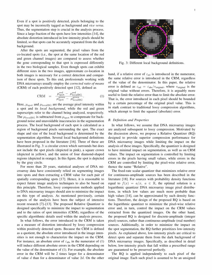
Here, µspot and µlocalBG are the average pixel intensity withina spot and its local background, while the red and greensuperscripts refer to the channel being analyzed, respectively.The µlocalBG is subtracted from µspot to compensate for back-ground noise and unavoidable inaccuracies in the segmentationprocess. The local background of each spot is calculated as aregion of background pixels surrounding the spot. The exactshape and size of the local background is determined by thesegmentation algorithm. Several local background definitionshave been proposed in the literature [16]. Three of these areillustrated in Fig. 3: a circular crown which surrounds but doesnot include the spot pixels (depicted in pink), a square crown(depicted in yellow), and the union of four diamond-shapedregions (depicted in orange). In this figure, the spot is depictedby the gray circle.

For more than 20 years, statistical analyses of DNA mi-croarray data have consistently relied on segmenting imagesinto spots and then extracting a CRM value for each pair ofspatially corresponding spots [17]. Hence, it is reasonable toexpect future image analysis techniques to also be based onthis principle. Therefore, lossy compression methods appliedto DNA microarray images should aim to minimize the impacton this type of analysis. As mentioned previously, certainaspects of the analysis have been the subject of intensiverecent research [7]–[13]. The proposed Relative Quantizer isdesigned specifically to minimize the impact to segmentationand to the ratios of spot intensities (CRM), regardless of thespecific algorithmic details used within the analysis process.

In what follows, the error introduced in the CRM is takenas a measure of distortion introduced by lossy compressionwithin positively detected spots. Because the CRM is definedas a quotient, the absolute error introduced in the image inten-sities is not enough to characterize the impact on the CRM.For instance, an absolute error of εabs in the numerator of (1)will induce different absolute errors in the CRM depending onthe value of the denominator of (1). For example, the absoluteerror in the CRM will be 2 times larger for a denominatorof value d than for a denominator of value 2d. On the other

Fig. 3: Different local background definitions.

hand, if a relative error of εrel is introduced in the numerator,the same relative error is introduced in the CRM, regardlessof the value of the denominator. In this paper, the relativeerror is defined as εrel = εabs/voriginal, where voriginal is theoriginal value without errors. Therefore, it is arguably moreuseful to limit the relative error than to limit the absolute error.That is, the error introduced in each pixel should be boundedby a certain percentage of the original pixel value. This isin stark contrast to traditional lossy compression algorithms,which attempt to limit the squared (absolute) error.

B. Definition and Properties

In what follows, we assume that DNA microarray imagesare analyzed subsequent to lossy compression. Motivated bythe discussion above, we propose a Relative Quantizer (RQ)designed to provide superior compression performance forDNA microarray images while limiting the impact on theanalysis of these images. Specifically, the quantizer is designedto have minimal impact on segmentation, as well as on CRMvalues. The impact on segmentation is controlled by limitingerrors in the pixels having small values, while errors in theCRM are controlled by limiting the pixel-wise relative error,thence the name “Relative”.

The fixed-rate scalar quantizer that minimizes relative errorfor continuous-amplitude sources has been described in theliterature [18]. For sources with probability density functionsequal to f(x) = a/x, a ∈ R, the optimal solution is alogarithmic quantizer DNA microarray image pixel distribu-tions, in which low values are much more probable thanhigh values [14], can be approximated by such density func-tions. Therefore, the design of the proposed RQ is based onthe logarithmic quantizer to minimize the pixel-wise relativeerror and, in turn, control the impact on the CRM valuesextracted from the quantized images. On the other hand,the proposed RQ is designed for discrete-amplitude (integerpixel) sources, rather than continuous-amplitude (real number)sources. Additionally, in order to minimize the impact onthe spot segmentation, the RQ further prioritizes low-intensitypixels. As explained above, low-intensity pixels are critical todetect spots and separate them from the dark background ofDNA microarray images. Specifically, as described in detailbelow, low-intensity pixels that fall within a prescribed rangeare guaranteed to be preserved perfectly.

The RQ is applied independently to each pixel of theoriginal image. Each such pixel is assumed to be an unsigned

4

TABLE I: Original pixel values (Orig.), quantization indices (QI) and reconstructed values (Rec.) for the RQ using B = 4and k = 2. Bits preserved in each value are highlighted in bold font. The interval midpoint rounded up is employed for thereconstruction.

Orig. 0 1 2 3 4 5 6 7 8 9 10 11 12 13 14 150000 0001 0010 0011 0100 0101 0110 0111 1000 1001 1010 1011 1100 1101 1110 1111

QI 0 1 2 3 4 4 5 5 6 6 6 6 7 7 7 7

Rec. 0000 0001 0010 0011 0101 0101 0111 0111 1010 1010 1010 1010 1110 1110 1110 11100 1 2 3 5 5 7 7 10 10 10 10 14 14 14 14

integer of bitdepth B ≥ 1. The RQ is parameterized by aninteger k in {1, . . . , B}. As explained in detail below, theparameter k determines the number of quantization intervalsand their size, which in turn controls the fidelity with whicheach individual pixel is preserved. Small values of k yield lowfidelity, while increasing k yields higher fidelity. Indeed, whenk = B, the size of all quantization intervals is exactly 1, so noquantization is applied, and all pixels are preserved perfectly.In order to describe the quantization intervals, it is useful toconsider pixel values in their binary representation. For a givenpixel, let N be the position of its most significant bit havingvalue equal to 1, where B − 1 and 0 are the most and leastsignificant positions, respectively. For example, let B = 4.Then pixels having values v1 = 00012, v2 = 01002 andv3 = 01012 have N1 = 0, N2 = 2 and N3 = 2, respectively.

The main idea of the RQ is to then preserve only the bits inpositions B− 1, . . . , N − k+1. Note that, by definition, onlythe k bits in positions N, ..., N − k+1, can be different from0. Thus, the parameter k effectively determines the maximumnumber of non-null bits that are preserved for each pixel. Fromthis observations, it follows that if N < k, then all bits ofthe pixels are preserved. That is, all pixels having values in{0, 1, . . . , 2k − 1} are preserved losslessly.

Table I shows the operation of the RQ for B = 4 andk = 2. The first two rows in the table show the decimaland binary representations for each possible pixel value. Thebits to be preserved are highlighted in bold font. Pixel valuesthat are identical in the preserved positions are assigned tothe same quantization interval, and hence, have the samequantization index, as given in the third row. The fourth andfifth rows show the binary and decimal representations of thereconstructed pixel values at the output of the dequantizer. Theinterval mid-point rounded up to the next integer has been usedfor reconstruction. As an example, two pixels taking values01002 and 01012 belong to the same quantization interval.They share a common quantization index of 4, and are bothreconstructed as 5. As expected, pixels having values less than2k = 4 are preserved perfectly.

As seen in Table I, when B = 4 and k = 2, there are 8distinct quantizer indices. To calculate the number of quantizerindices for arbitrary B and k, it is illustrative to view the RQas a quantizer having non-uniform intervals. For any choice ofB, the first 2k intervals correspond to preserving all bits of anypixel having value 0 ≤ p < 2k. Each interval thus containsonly one value. That is, each interval is of size 20 = 1. Thenext 2k−1 intervals correspond to preserving all but the leastsignificant bit of any pixel with value 2k ≤ p < 2k+1. Hence,

two values are assigned to each interval. That is, each intervalis of size 21. The next 2k−1 intervals correspond to preservingall but the two least significant bits of any pixel with value2k+1 ≤ p < 2k+2. Each such interval is of size 22. Eachsubsequent group of 2k−1 intervals has size 23, 24, etc. Finally,the 2k−1 intervals of the last group each have size 2B−k. Thislast group of intervals preserves the k most significant bits ofany pixel having value 2B−1 ≤ p < 2B .

For any values of B and k, the exact number of quantizationintervals Ik can then be easily calculated. Since there are 2k

intervals of size 1 and 2k−1 intervals of each size s with s ∈{21, 22, . . . , 2B−k}, there are exactly 2k + (B − k)2k−1 =(B − k + 2)2k−1 quantization intervals. Table II provides Ikfor several values of B and k.

TABLE II: Number of quantization intervals Ik for the RQusing B = 4 and B = 16.

k 1 2 3 4 5 6 7Ik (B = 4) 5 8 12 16 N/A N/A N/AIk (B = 16) 17 32 60 112 208 384 704

In summary, no error is incurred in the 2k lowest pixelvalues. Additionally, several of the next quantization intervalgroups have small lengths: 2, 4, 8, 16, etc., implying smallmaximum errors. As discussed in Section II-A, low intensitypixels are crucial for the spot segmentation. Thus, the smallmaximum error introduced by the RQ in this intensity rangeattenuates the impact on the segmentation process. Moreover,the maximum relative error in each pixel is bounded. Specifi-cally, pixels having values 2k+j ≤ p < 2k+j+1 are quantizedusing an interval of size exactly 2j+1, j = 0, 1, . . . , B−(k+1).It follows that the absolute error introduced in a pixel byquantization/dequantization is at most εabs = 2j , so that themaximum relative error is bounded by εrel = 2j/2k+j = 2−k.As explained in Section II-A, limiting the pixel-wise relativeerror helps control the distortion in the extracted CRM values.Note that this approach is not specifically designed for anyconcrete DNA microarray image analysis algorithm. Instead,the Relative Quantizer relies on preserving the intensity ratios,and not on the specific way in which a particular algorithmsegments the images. Hence, using the proposed approach isreasonable for any existing or future analysis algorithm basedon the CRM.

5

III. IMPACT OF THE RELATIVE QUANTIZER ON GENETICDATA EXTRACTION

A. Distortion Metrics

The main drawback of lossy coding methods applied toDNA microarray images is the possibility of distorting theresults of any subsequent genetic data extraction process. Asexplained in Section II-A, the segmentation step may fail todetect one or more spots. Also, the corrected ratio of means(CRM) values extracted for positively detected spots may bedistorted.

CRM values are usually classified into one of three cate-gories: a) CRM < α, b) CRM > β or c) CRM ∈ [α, β].Typically, α = 0.5 and β = 2 [3], so that if CRM < 1/2for a given spot (Category a)), then the gene associated withthat spot is declared to be more strongly expressed in the“green sample” (that is, the biological sample associated withthe green florescent marker) than in the red sample. Indeed,CRM < 1/2 implies that the denominator of Eq (1) is morethan twice as large as the numerator. Similarly, if CRM > 2(Category b)), then the gene is declared to be more stronglyexpressed in the red sample. Finally, Category c) indicates thatthe gene is expressed roughly equally in both samples. Thisclassification is usually the only output considered, and expertsfrom the Genomics and Bioinformatics Service of the Biologyand Biomedicine Institute (IBB) at the Universitat Autonomade Barcelona (UAB) agree that any lossy process for which nodetection errors occur and the extracted CRM values remainunmodified is equivalent to a numerically lossless process.

In practice, most CRM values are close to 1, and the fractionof spots whose CRM lies outside [α, β] is relatively small anddepends on the type of biological samples being compared.A histogram of the CRM values extracted from the positivelydetected spots of all 22 image pairs of the IBB corpus is shownin Fig. 4. As reported later in Table IV, the average numberof spots in the IBB set is about 14,000. For visualizationpurposes, all values smaller than -1 are considered to beexactly -1, and all values larger than 5 are considered to beexactly 5. Note that according to the CRM definition of (1),negative CRM values can occur when the average intensity ofthe local background is larger than the average intensity of thespot pixels.

Based on this, two full-reference distortion metrics aredefined below to assess the acceptability of the changesintroduced in the images by lossy processes, including theproposed RQ. The first one is the average relative error inthe CRM (ARECRM). Given the analysis results of an originaland a distorted (e.g., quantized) image pair, it is defined as

ARECRM =1

n

n∑i=1

|CRMi − CRMi|δ + |CRMi|

. (2)

Here, n is the number of spots positively detected in boththe original and the distorted image pairs. The CRM extractedfrom the i-th such spot in the original and distorted imagepairs are denoted as CRMi and CRMi, respectively. Theparameter δ is set to 0.001 to stabilize the case CRMi = 0.As an example, a value of ARECRM = 0.5 would indicatethat, on average, the distorted CRM values differ by 50% of

1 0 1 2 3 4 5CRM

0.00

0.01

0.02

0.03

0.04

0.05

0.06

Prob

abilit

y

Fig. 4: Distribution of the CRM values extracted from all 22original image pairs of the IBB corpus.

their original values. This metric provides insight on the globaldistortion in the analysis process. Similar analysis distortionmetrics have been employed in the literature [1], [2].

The second metric is the fraction of spots wrongly detectedor classified (FWDOC). It is defined as

FWDOC = (d+ c)/m, (3)

where d is the number of spots that are detected differentlyin the original and quantized image pairs, c is the numberof spots that are positively detected in both the original andquantized image pairs but are classified differently, and m isthe total number of spots. Here, a spot is considered to bedetected differently if it is positively detected in the originalimage pairs but not in the quantized image pairs, or viceversa. Note that m includes both positively detected and notpositively detected spots and, hence, m ≥ n. Similar ap-proaches have been used in [2] and [3]. This metric quantifiesthe probability of a spot becoming unusable because of theintroduced distortion. As suggested by the IBB experts, theinterval R = [α, β] = [0.5, 2] is employed in this work toperform all classification operations.

B. Distortion Results

A number of tests have been carried out to evaluate theperformance of the RQ with respect to microarray images. Thefirst such test was to evaluate the distortion resulting from theRQ for various values of k. This test was performed using acorpus of 44 images (22 red/green image pairs), obtained fromreal experiments at the IBB, hereinafter referred to as the IBBcorpus. Specifically, all images from the corpus were quantizedby the proposed RQ using k ∈ {1, . . . , 7}. The images werethen reconstructed from quantization indices by employinginterval mid-points rounded up to the next integer. The originalIBB corpus and the 7 reconstructed versions were analyzedwith the GenePix software at the IBB [19]. The results for theoriginal and the quantized versions were compared using thetwo metrics described in Section III-A.

In the IBB corpus, each spot is replicated, i.e., there are2 spots devoted to each gene. Ideally, identical segmentationand CRM results should be obtained for both spots. However,

6

in real experiments, they differ even in the original imagesbefore quantization. Thus, two more metrics have been derivedfrom (2) and (3) to calculate the variability present betweenpairs of replicated spots in the original images. Given the anal-ysis results of an original image pair, the replicate ARECRM

(Rep-ARECRM) is defined as

Rep-ARECRM =1

p

p∑i=1

|CRMfi − CRMs

i |δ + |CRMf

i +CRMsi |/2

, (4)

where CRMfi and CRMs

i are, respectively, the CRM of thefirst and second spots of the i-th replicated spot pair, p isthe number of such spot pairs where both spots are positivelydetected, and δ = 0.001. Similarly, the replicate fraction ofspots wrongly detected or classified (Rep-FWDOC) is definedas

Rep-FWDOC = (dpair + cpair)/q, (5)

where dpair and cpair are the number of pairs whose spots aredifferently detected or classified, respectively, and q is thetotal number of pairs in the image. Since not all spots arenecessarily detected, q ≥ p.

Results for the quantized images and for the replicatedspots in the original images are provided in Table III. Inthe most aggressive case (k = 1), large errors are apparent,especially in the ARECRM. Nevertheless, rapid improvementis observed as the parameter k is increased. For k ≥ 4,the ARECRM and the FWDOC are below 8.0% and 4.5%,respectively. Significantly, for all k > 1, the ARECRM andthe FWDOC metrics show a better behavior than the Rep-ARECRM and the Rep-FWDOC for the replicated spots in theoriginal images. In the literature on lossy compression of DNAmicroarray images, distortions smaller than the experimentalvariability are considered acceptable [1]–[3]. The distortionamong replicated spots can be understood as a measure of thisvariability. In this light, the results of Table III suggest thatthe proposed RQ yields acceptable distortions for all k > 1.

Arguably, the selection of a suitable value for k might bespecific to the scanner and analysis software employed. Givena set of images and analysis software appropriate for thescanner from which the images were acquired, a conservative

TABLE III: Average relative error in the CRM (ARECRM) andfraction of spots wrongly detected or classified (FWDOC) afterthe RQ. Results have been averaged over all 22 image pairs ofthe IBB corpus. Average data for the pairs of replicated spotsin the original images (the Rep-ARECRM and Rep-FWDOCmetrics) are provided at the bottom.

Images ARECRM FWDOCOriginal vs. RQ k = 1 0.562 0.148Original vs. RQ k = 2 0.124 0.100Original vs. RQ k = 3 0.121 0.064Original vs. RQ k = 4 0.078 0.044Original vs. RQ k = 5 0.064 0.030Original vs. RQ k = 6 0.039 0.019Original vs. RQ k = 7 0.028 0.014

Images Rep-ARECRM Rep-FWDOCOriginal 0.254 0.212

approach might be to select a value of k for which the averagedistortion measured by the metrics proposed in (2) and (3) arebetween one half and one third of the replicate variability asdefined in (4) and (5), respectively. For the IBB corpus and theGenePix analysis software, this leads to the choice of k = 3or k = 4.

Results for the test described in this section have not beenobtained for DNA microarray images from other corpora.Other corpora employed in the literature either do not consistof green/red channel pairs from the same DNA microarrayexperiment, or no compatible analysis software is publiclyavailable. Thus, an exhaustive study on the impact of k onthe analysis of such corpora is beyond the scope of thiswork. Nevertheless, the properties of the RQ described inSection II-B (bounded relative error for all pixels and smallabsolute error for low-intensity pixels) do not depend on thesource of the image being quantized. Moreover, since themaximum relative error of 2−k quickly decreases as k isincreased, it is reasonable to expect the analysis distortion tobe a monotonically decreasing function of k for any image set,and that a very small analysis distortion should be obtainedfor any image whenever k > 5.

Additional tests that employ the IBB corpus, as well as othercorpora from the literature, are discussed in the next section.

IV. LOSSLESS CODING OF RQ INDICES

The previous section characterized the distortion introducedto DNA microarray images by the proposed RQ as a functionof the parameter k. In this section, compression performanceis discussed. To this end, several techniques for storing the RQindices of quantized images are investigated. These techniquescan be considered as lossless coding (or compression). Foreach technique, the RQ indices can be recovered exactly, andthus the distortion introduced into the images is entirely in-dependent of the lossless coding technique employed. Indeed,the resulting decompressed images are identical for each andevery technique. The only difference between the differinglossless compression techniques is the resulting compressionperformance. In what follows, compression performance isreported in terms of the average rate R in bits per pixel (bpp)required to store the indices of an image. This quantity canbe converted into compression ratio for a 16-bit image asCR = 16/R.

A. DNA Microarray Image Corpora

A total of 228 DNA microarray images in 7 corporaproduced by different types of scanners have been gathered toevaluate the lossless compression of indices produced by theproposed RQ. All images most often used for benchmarkingin the DNA microarray image compression literature –theYeast, the ApoA1, the ISREC, the Stanford and the MicroZipcorpora– have been included. Additionally, the Arizona andIBB corpora, which contain images representative of theoutput of more modern DNA microarray scanners, have beenincluded. Table IV summarizes some of the most impor-tant image characteristics. In particular, the total number ofgrayscale images in each corpus is provided in the Images

7

TABLE IV: Image corpora used for benchmarking in this work. Original image pixels are unsigned 16-bit integers.

Property Yeast [20] ApoA1 [21] ISREC [22] Stanford [23] MicroZip [4] Arizona [24] IBB [25]Year 1998 2001 2001 2001 2004 2011 2013Images 109 32 14 20 3 6 44Size 1024×1024 1044×1041 1000×1000 > 2000×2000 > 1800×1900 4400×13800 2019×6235Spot count ∼ 9 · 103 ∼ 6 · 103 ∼ 2 · 102 ∼ 4 · 103 ∼ 9 · 103 ∼ 2 · 105 ∼ 1.4 · 104Avg. intensities 5.39% 39.51% 33.34% 28.83% 37.71% 82.82% 54.07%Avg. entropy (bpp) 6.628 11.033 10.435 8.293 9.831 9.306 8.503Best rate (bpp) [26] 5.521 10.223 10.199 7.335 8.667 8.275 8.039

row. All images are 16 bpp. Some of the corpora do notcontain green/red channel pairs, which yields an odd numberof grayscale images in some cases. Along with the spatialsize for each corpus, the average number of spots in eachimage of a given corpus is reported in the Spot count row.The percentage of the 216 possible pixel intensity values thatare actually present in each image has been computed, andthe average percentage for each corpus is reported in the Avg.intensities row. The average first-order entropy of each corpusis reported in the row labeled Avg. entropy. Results for the bestmethod known for lossless DNA microarray compression [26]are expressed in terms of bpp in the last row. These resultswere obtained for the original unquantized images using animplementation provided by the authors of [26]. For eachcorpus, the reported results are better than the first-orderentropy, due to the fact that pixel dependencies are effectivelyexploited by the coding method employed.

B. Compression Experiments

All images from the described corpora were quantized bythe proposed Relative Quantizer (RQ) and the quantization in-dices were stored as an image. Each resulting index image wasthen subjected to lossless compression using several losslessalgorithms. As mentioned previously, each of these algorithmsmay yield a different value for compression performance (inbpp). However, the resulting image distortion (and indeed, theimages themselves) will be identical for each algorithm. Thisexperiment was performed for each value of k ∈ {1, 2, . . . , 7}.Since k = 7 already yields analysis distortions 10 to 20 timessmaller than the experimental variability (see Section III-B),larger values of k have not been considered here.

The tested lossless coding algorithms include genericdata compressors (bzip2), image and video compressorsnot specifically designed for DNA microarrays (JPEG-LS [27], CALIC [28], lossless JPEG2000 [29] and losslessHEVC/H.265 [30]), and the best lossless microarray-specificimage compressor (Neves and Pinho’s method [26]). Unlessstated otherwise, all codecs were invoked with default pa-rameters. The HEVC coder was invoked using coding unitsize equal to 64× 64, and bypassing the lossy stages (whichwould be enabled by default). For the HEVC experiments, allimages were stored using YUV 4:2:2 format, with the U andV components being exactly zero. The exact configuration pa-rameters employed for HEVC are available at http://deic.uab.es/∼mhernandez/media/software/hevc lossless.cfg. Note thatpublicly available CALIC codecs support only images up to8 bpp, i.e., 256 different pixel values. As can be seen from

Table II, the proposed RQ yields index images with 384 ormore intensities whenever k ≥ 6. Therefore, CALIC has onlybeen applied for k < 6. The H.264 standard has not beenincluded in this study since it does not support image sizeslarge enough for many DNA microarray images [31].

In addition to the variable-rate methods listed in the previousparagraph, fixed-rate coding is also considered. The simplestsuch strategy is to assign to each index a fixed length codewordof length dlog2 Ike bits. For example, when k = 4 (and B =16), a codeword length of dlog2 112e = 7 bits will suffice.If a block of L indices are coded together, a codeword oflength dlog2 ILk e will suffice. The rate of the resulting codeis then 1

Ldlog2 ILk e < log2 Ik + 1

L . Thus, fixed length codingcan approach log2 Ik bits per pixel as closely as desired.

Table V presents the results obtained for each value ofk by the different coding techniques. Data for the originalimages before quantization is also provided. Results are givenin bits per pixel, calculated as the combined size in bits of allcompressed images divided by the total number of pixels ina corpus. The fixed-rate results do not depend on the corpusand are reported once at the top of the table for block sizeL = 2000. The Lossless JPEG2000 row contains results forKakadu v7.4 using the best choice of parameters for eachcolumn1.

As expected, the bitrate decreases (compression ratio in-creases) as k is decreased for all tested coders. For example,bitrate reductions of over 20% are observed for k = 7, ascompared to the original images. As another example, 60%reductions are observed for k = 3. For a specific corpusand specific value of k, the rates resulting from differentcoders are typically within 0.5 bits per pixel, with severalnotable exceptions. For example, the state-of-the-art videocoder HEVC/H.265 produces very poor results for the originalimages, but provides more competitive performance for RQindex images. For every value of k, the best-performing coderfor all image corpora is that of Neves and Pinho [26]. Thisshould be expected, at least for the case of the original DNAmicroarray images, for which it was designed. Therefore,Neves’ method is hereinafter used to losslessly code the quan-tization indices produced by the proposed Relative Quantizer.

C. Rate-distortion Analysis

The previous sections have demonstrated that compressionsystems based on the proposed RQ can provide significant

1Ssigned=no and 0 wavelet decomposition levels for 1 ≤ k ≤ 4;Ssigned=no and 3 DWT decomposition levels for 5 ≤ k ≤ 6; Ssigned=yesand 0 DWT decomposition levels for k = 7 and for the original images.

8

TABLE V: Compression results in bpp for RQ followed by different lossless coding algorithms. Lossless compression resultsfor the original images are also provided.

Corpus Algorithm RQ index images Original imagesk = 1 k = 2 k = 3 k = 4 k = 5 k = 6 k = 7

Fixed-length coder 4.087 5.000 5.907 6.807 7.700 8.585 9.459 16.000

Yeast

Average entropy 1.854 2.474 3.272 4.156 5.074 5.945 6.294 6.628bzip2 1.028 1.614 2.462 3.399 4.355 5.250 5.655 6.075JPEG-LS 1.007 1.497 2.231 3.082 3.986 4.989 5.892 8.580CALIC 0.977 1.503 2.268 3.075 3.940 – – –Lossless JPEG2000 1.355 1.473 2.282 3.417 4.339 5.308 6.219 5.903HEVC/H.265 1.241 1.844 2.632 3.532 4.495 5.532 6.650 10.660Neves & Pinho 0.900 1.339 2.017 2.921 3.887 4.769 5.056 5.511

ApoA1

Average entropy 1.704 2.504 3.442 4.423 5.417 6.415 7.414 11.033bzip2 1.357 2.121 3.062 4.052 5.063 6.090 7.106 11.064JPEG-LS 1.258 1.921 2.746 3.691 4.680 5.728 6.698 10.606CALIC 1.202 1.889 2.729 3.620 4.588 – – –Lossless JPEG2000 1.404 1.930 2.822 3.758 4.859 5.896 7.518 10.787HEVC/H.265 1.348 2.054 2.943 3.936 5.009 6.168 7.408 14.482Neves & Pinho 1.041 1.715 2.604 3.565 4.562 5.557 6.565 10.223

ISREC

Average entropy 2.674 3.617 4.597 5.585 6.543 7.442 8.277 10.435bzip2 2.681 3.621 4.604 5.599 6.561 7.476 8.373 10.921JPEG-LS 2.725 3.671 4.663 5.660 6.670 7.601 8.494 11.145CALIC 2.639 3.526 4.482 5.471 6.464 – – –Lossless JPEG2000 2.690 3.518 4.536 5.575 6.703 7.695 8.491 10.625HEVC/H.265 2.623 3.618 4.705 5.880 7.102 8.503 10.077 14.876Neves & Pinho 2.403 3.317 4.291 5.281 6.241 7.144 7.976 10.199

Stanford

Average entropy 2.021 2.863 3.801 4.785 5.777 6.662 7.268 8.293bzip2 1.415 2.205 3.107 4.090 5.098 5.982 6.553 7.887JPEG-LS 1.343 1.974 2.839 3.802 4.796 5.700 6.241 7.597CALIC 1.230 2.003 2.786 3.701 4.678 – – –Lossless JPEG2000 1.524 2.048 3.053 4.120 4.946 5.865 6.589 7.685HEVC/H.265 1.373 2.051 2.958 3.952 5.024 6.034 6.702 8.897Neves & Pinho 1.105 1.793 2.695 3.653 4.659 5.512 6.053 7.335

Microzip

Average entropy 1.859 2.729 3.679 4.665 5.662 6.661 7.639 9.831bzip2 1.574 2.435 3.380 4.370 5.381 6.408 7.379 9.394JPEG-LS 1.448 2.149 3.037 4.013 5.011 6.028 7.005 8.974CALIC 1.383 2.176 2.977 3.915 4.904 – – –Lossless JPEG2000 1.825 2.161 3.178 4.275 5.171 6.212 7.597 9.157HEVC/H.265 1.609 2.403 3.339 4.343 5.447 6.638 7.893 11.179Neves & Pinho 1.243 1.957 2.864 3.868 4.856 5.859 6.830 8.667

Arizona

Average entropy 2.094 2.959 3.902 4.887 5.881 6.877 7.781 9.306bzip2 1.577 2.398 3.321 4.304 5.309 6.331 7.234 8.944JPEG-LS 1.491 2.270 3.139 4.102 5.093 6.125 7.005 8.646CALIC 1.464 2.250 3.061 4.003 4.980 – – –Lossless JPEG2000 1.742 2.216 3.273 4.351 5.241 6.274 7.424 8.795HEVC/H.265 1.470 2.280 3.229 4.236 5.338 6.532 7.664 10.592Neves & Pinho 1.201 1.976 2.874 3.878 4.870 5.867 6.766 8.275

IBB

Average entropy 3.168 3.906 4.651 5.386 6.095 6.756 7.340 8.503bzip2 3.048 3.832 4.649 5.448 6.206 6.927 7.590 9.081JPEG-LS 3.571 4.490 5.373 6.227 7.029 7.733 8.429 9.904CALIC 3.366 4.235 5.091 5.936 6.740 – – –Lossless JPEG2000 3.179 3.880 4.788 5.646 7.271 8.076 7.261 8.392HEVC/H.265 3.654 4.671 5.685 6.716 7.717 8.863 9.991 12.262Neves & Pinho 2.653 3.363 4.105 4.844 5.556 6.214 6.800 8.039

Corpora averages

Average entropy 2.196 3.007 3.906 4.841 5.778 6.680 7.430 9.010bzip2 1.817 2.610 3.519 4.473 5.432 6.362 7.148 9.052JPEG-LS 1.835 2.567 3.433 4.368 5.324 6.272 7.109 9.350CALIC 1.752 2.512 3.342 4.246 5.185 – – –Lossless JPEG2000 2.006 2.745 3.596 4.532 5.511 6.483 7.392 9.759HEVC/H.265 1.903 2.703 3.642 4.656 5.733 6.896 8.055 11.850Neves & Pinho 1.507 2.209 3.064 4.001 4.947 5.846 6.578 8.321

9

2.5 3.0 3.5 4.0 4.5 5.0 5.5 6.0 6.5 7.0

Rate (bpp)

40

50

60

70

80

90PS

NR

(d

B)

Lossy JPEG2000

Near-lossless JPEG-LS

HEVC

RQ + Neves

k=1 k=2

k=3

k=4

k=5

k=6

k=7

R=3

R=4

R=5

R=6

R=7

e=32

e=16

e=8

QP=5

QP=4

QP=1

(a)

0.0 0.2 0.4 0.6 0.8 1.0ARECRM

30

40

50

60

70

80

90

100

PSNR

(dB)

Lossy JPEG2000Near-lossless JPEG-LS

HEVCRQ + Neves

(b)

Fig. 5: Evaluation of the PSNR metric. (a) PSNR as a functionof the average compression bitrate; (b) PSNR as a function ofthe ARECRM metric.

compression with negligible effect on the DNA microarrayanalysis. In what follows, we compare the performance of RQ-based compression with other lossy compression approaches,using the distortion metrics developed in Section III.

As discussed in Section II-A, metrics based on the quadraticpixel-wise error like the PSNR (or MSE) are not adequatein this regard. Similarly, metrics based on the human visualsystem such as SSIM [32] and HDR-VDP 2 [33] may not beuseful, since microarray images are analyzed by algorithmsand not by human observers. Nevertheless, it is of interest toexamine the results for these metrics yielded by the algorithmsof interest. To this end, images from the IBB corpus werecompressed with lossy JPEG20002 compression for targetbitrates R ∈ 3, 4, . . . , 7, near-lossless JPEG-LS compressionfor maximum absolute error e ∈ {4, 16, 32, 64}3, lossy HEVCwith quality parameter QP ∈ {1, 4, 5} and the proposed RQfor k ∈ {1, 2, . . . , 7}. Note that current rate-control algorithmsfor HEVC are not designed for intra-coding of a single pic-

2Without applying the level offset and using 3 levels of the 9/7 irreversibleDWT, the best choice for this corpus.

3Using parameters -ls 0 -m e.

ture [34]. Their accuracy in yielding a target bitrate is usuallylow, hence only the QP is used here. Each parameter choicefor each algorithm yields a different compression treatment.When applied to the entire corpus, each such treatment yieldsan average PSNR and average compression performance (ratein bpp). Each such PSNR/rate pair is plotted in Fig. 5a. Eachalgorithm is represented by a different color in the figure.Each parameter choice is labeled next to its correspondingPSNR/rate pair. It can be seen that the proposed method yieldslower PSNR results than lossy JPEG2000, near-lossless JPEG-LS and lossy HEVC. This is as expected since those algorithmsconsider the absolute error in each pixel. This is exactly theerror targeted by traditional metrics such as MSE/PSNR. Onthe other hand, the proposed Relative Quantizer preserves thesmaller pixel values more carefully while tolerating largererrors in pixels having large values.

To emphasize that PSNR is not a good predictor of the errorsincurred in the CRM, all PSNR/ARECRM pairs are depicted inFig. 5b. Each point of this graph corresponds to one image ofthe IBB corpus, one algorithm and one parameter value. Thecolor of each marker identifies the algorithm employed, anddifferent parameter values are denoted with different markershapes. It can be observed that the PSNR is not well correlatedwith the relative error introduced in the extracted CRM.Similar results are obtained for the MSE, SSIM and HDR-VDP-2 metrics. Therefore, only the ARECRM and FWDOCmetrics defined in Section III-A are employed for the resultsthat follow.

To the best of the authors’ knowledge, all lossy algo-rithms published in 2004 or earlier [1], [2], [4] are basedon either lossy JPEG2000 or near-lossless JPEG-LS. Twomicroarray-specific lossy compression methods [5], [6] havebeen published since then. The results reported in [5] are morethan 5 dB worse than JPEG2000 in terms of PSNR. Usingthe authors implementation of the wavelet-fractal algorithmreported in [6], we obtained ARECRM and FWDOC resultsof 1.030 and 0.286, respectively. The results of the proposedRQ method are significantly better for every value of k. Inlight of these results, only the standard lossy JPEG2000,lossy HEVC and near-lossless JPEG-LS algorithms are usedto provide comparisons with the proposed RQ-based coder. Inthese comparisons, Neves and Pinho’s algorithm is used forlossless compression of the RQ indices.

The resulting rate-distortion curves for the IBB corpus areshown in Fig. 6. Results for the lossy JPEG2000 algorithmhave been obtained without applying the level offset and using3 decomposition levels of the 9/7 irreversible DWT, the bestchoice for this corpus.

It can be observed that for k > 1, the proposed systemconsistently yields better results than lossy JPEG2000, near-lossless JPEG-LS and lossy HEVC for both the ARECRMand FWDOC metrics. Notice that for QP = 1, lossy HEVCproduces worse distortion results than the proposed RQ withk = 2, and that, as explained above, QP = 1 corresponds tothe maximum quality for lossy HEVC and it is not possibleto generate results for higher bitrates using this algorithm.At about only 3.4 bpp, the proposed algorithm produces lessthan Rep-ARECRM / 2 and Rep-FWDOC / 2, i.e., half the

10

3 4 5 6 7Bitrate (bpp)

0.00

0.05

0.10

0.15

0.20

0.25

0.30

0.35

0.40

ARECRM

Rep−ARECRM / 2Rep−ARECRM / 2Rep−ARECRM / 2Rep−ARECRM / 2

Lossy JPEG2000

Near-lossless JPEG-LS

Lossy HEVC

RQ + Neves

k=7k=6k=5

k=4

k=3k=2

R=7R=6

R=5

R=4

R=3

e=4

e=16

e=32

QP=1QP=4

QP=5

(a)

3 4 5 6 7Bitrate (bpp)

0.00

0.05

0.10

0.15

0.20

FW

DO

C

Rep−FWDOC / 2Rep−FWDOC / 2Rep−FWDOC / 2Rep−FWDOC / 2

Lossy JPEG2000

Near-lossless JPEG-LS

Lossy HEVC

RQ + Neves

k=1

k=2

k=3

k=4k=5

k=6 k=7

R=7

R=6

R=5

R=4

R=3QP=5QP=4

QP=1

e=4

e=16

e=32

(b)

Fig. 6: Distortion metrics versus bitrate: (a) average relative error in the CRM (ARECRM); (b) fraction of spots incorrectlydetected or classified (FWDOC). Half the average replicate CRM relative error (Rep-ARECRM/2) and half the fraction ofreplicated spots wrongly detected or classified (Rep-FWDOC / 2) are shown as horizontal lines in (a) and (b), respectively.

acceptable experimental variability. This should be comparedto an average of 8.039 bpp required to achieve strictly losslesscompression of the original images without quantization (ascan be seen in Table V).

The sudden increase in ARECRM for JPEG2000 in Fig. 6afor target bitrate R = 5 bpp is due to a small number of verylarge errors introduced into the CRM by JPEG2000 at that bitrate. In particular, 10 spots belonging to 3 different imageshave relative errors of more than 1000 after compression withJPEG2000. The sudden increase observed in Fig. 6a is dueentirely to these 10 spots. The behavior of JPEG2000 can beexplained by noting that when the denominator of Eq. (1) issmall, even small changes in the numerator or the denominatorcan cause large errors in the CRM. JPEG2000 makes noattempt to account for this issue. On the other hand, thisbehavior is not present in the proposed RQ, since the errorintroduced in the CRM is strictly limited by construction.

V. CONCLUSIONS

DNA microarray images are usually stored so that they canbe re-analyzed with future algorithms or in different labora-tories. Due to the large amount of DNA microarray imageinformation being currently generated, image compression isa useful tool to cope with the storage and transmission of thesedata. State-of-the-art lossless coding algorithms typically yieldcompression ratios of only 2:1 or less. Lossy coding methodscan attain much higher compression ratios, however, somedistortion is introduced in the decompressed images. Thus,it is necessary to assess the acceptability of this distortion inregards to subsequent image analysis.

In this paper, a Relative Quantizer (RQ)-based lossy com-pression method is proposed. The RQ is designed to limit twoquantities that are crucial to the analysis process: the relativeerror of all pixels and the absolute error of low-intensitypixels. The distortion introduced by the proposed RQ resultsin errors in the analysis process that are smaller than those dueto the experimental variability inherent to DNA microarrays.The proposed coding algorithm results in compression ratiosexceeding 4.5:1 without introducing any additional analysiserror. Furthermore, the k parameter of the RQ can be adjustedto trade off compression bitrate for analysis result precision.The rate-distortion results of the proposed coder significantlyoutperform those of state-of-the-art lossy coding algorithms.

ACKNOWLEDGMENTS

The Arizona corpus was provided by Prof. D. Galbraithand Dr. M. Sweeney from the University of Arizona. The IBBcorpus was provided by A. Barcelo and A. Casamayor fromthe Genomics and Bioinformatics Service of the IBB at theUAB, whom the authors also thank for providing expertise onDNA microarrays.

REFERENCES

[1] R. Jornsten, W. Wang, B. Yu, and K. Ramchandran, “Microarrayimage compression: SLOCO and the effect of information loss,” SignalProcessing, vol. 83, no. 4, pp. 859–869, April 2003.

[2] J. Hua, Z. Liu, Z. Xiong, Q. Wu, and K. Castleman, “MicroarrayBASICA: Background Adjustment, Segmentation, Image Compressionand Analysis of microarray images,” EURASIP Journal on AppliedSignal Processing, vol. 2004, no. 1, pp. 92–107, January 2004.

[3] Q. Xu, J. Hua, Z. Xiong, M. L. Bittner, and E. R. Dougherty, “The effectof microarray image compression on expression-based classification,”Signal Image and Video Processing, vol. 3, no. 1, pp. 53–61, February2009.

11

[4] S. Lonardi and Y. Luo, “Gridding and compression of microarrayimages,” in Proceedings of the IEEE Computational Systems Bioinfor-matics Conference, 2004, pp. 122–130.

[5] T. J. Peters, R. Smolikova-Wachowiak, and M. P. Wachowiak, “Mi-croarray image compression using a variation of singular value decom-position,” in Proceedings of the Annual International Conference of theIEEE Engineering in Medicine and Biology Society, vol. 1-16, 2007, pp.1176–1179.

[6] M. R. N. Avanaki, A. Aber, and R. Ebrahimpour, “Compression ofcDNA microarray images based on pure-fractal and wavelet-fractaltechniques,” ICGST International Journal on Graphics, Vision andImage Processing, GVIP, vol. 11, pp. 43–52, March 2011.

[7] K. Blekas, N. Galatsanos, A. Likas, and I. Lagaris, “Mixture ModelAnalysis of DNA Microarray Images,” IEEE Trans. Med. Imag., vol. 24,no. 7, pp. 901–909, Jul. 2005.

[8] J. Ho and W.-L. Hwang, “Automatic Microarray Spot SegmentationUsing a Snake-Fisher Model,” IEEE Trans. Med. Imag., vol. 27, no. 6,pp. 847–857, Jun. 2008.

[9] E. Zacharia and D. Maroulis, “An Original Genetic Approach to theFully Automatic Gridding of Microarray Images,” IEEE Trans. Med.Imag., vol. 27, no. 6, pp. 805–812, Jun. 2008.

[10] L. Rueda and I. Rezaeian, “A fully automatic gridding method for cDNAmicroarray images,” BMC Bioinformatics, vol. 12, no. 1, p. 113, 2011.

[11] G.-F. Shao, F. Yang, Q. Zhang, Q.-F. Zhou, and L.-K. Luo, “Usingthe maximum between-class variance for automatic gridding of cDNAmicroarray images,” IEEE/ACM Trans. Comput. Biol. Bioinformatics,vol. 10, no. 1, pp. 181–192, Jan 2013.

[12] L. Rueda, Ed., Microarray image and data analysis: theory and practice.CRC Press, 2014.

[13] L. Srinivasan, Y. Rakvongthai, and S. Oraintara, “Microarray imagedenoising using complex Gaussian scale mixtures of complex wavelets,”IEEE J. Biomed. Health. Inform., vol. 18, no. 4, pp. 1423–1430, 2014.

[14] M. Hernandez-Cabronero, M. W. Marcellin, and J. Serra-Sagrista,“Compression of DNA microarray images,” in Microarray image anddata analysis: theory and practice. CRC Press, 2014, pp. 193–222.

[15] Y. Luo and S. Lonardi, “Storage and transmission of microarray images,”Drug Discovery Today, vol. 10, no. 23-24, pp. 1689 – 1695, 2005.

[16] Y. H. Yang, M. J. Buckley, and T. P. Speed, “Analysis of cDNAmicroarray images,” Briefings in Bioinformatics, vol. 2, no. 4, pp. 341–349, Jan. 2001.

[17] M. Schena, D. Shalon, R. W. Davis, and P. O. Brown, “Quantitativemonitoring of gene expression patterns with a complementary DNAmicroarray.” Science, vol. 270, no. 5235, pp. 467–470, 1995.

[18] J. Sun and V. Goyal, “Scalar quantization for relative error,” in Proceed-ings of the IEEE International Data Compression Conference, DCC,March 2011, pp. 293–302.

[19] Molecular Devices, “GenePix Pro [Online]. Availablehttp://moleculardevices.com/.”

[20] Y. Zhang, R. Parthe, and D. Adjeroh, “Lossless compression of DNAmicroarray images,” in Proceedings of the IEEE Computational SystemsBioinformatics Conference, August 2005, pp. 128 – 132.

[21] Speed Berkeley Research Group, “ApoA1 corpus [Online]. Downloadedfrom stat.berkeley.edu/users/terry/zarray/Html/apodata.html.”

[22] SIB Computational Genomic Group, “ISREC corpus [Online]. Down-loaded from: http://www.isrec.isb-sib.ch/DEA/module8/P5 chip image/images/.”

[23] Stanford Microarray Database, “Stanford corpus [Online]. Downloadedfrom: ftp://smd-ftp.stanford.edu/pub/smd/transfers/Jenny.”

[24] David Galbraith Laboratory, “Arizona corpus [Online]. Available: http://deic.uab.es/∼mhernandez/materials.”

[25] IBB Genomics Service, “IBB corpus [Online]. Available: http://deic.uab.es/∼mhernandez/materials.”

[26] A. J. R. Neves and A. J. Pinho, “Lossless compression of microarrayimages using image-dependent finite-context models,” IEEE Trans. Med.Imag., vol. 28, no. 2, pp. 194–201, February 2009.

[27] M. J. Weinberger, G. Seroussi, and G. Sapiro, “The LOCO-I losslessimage compression algorithm: principles and standardization into JPEG-LS,” IEEE Trans. Image Process., vol. 9, no. 8, pp. 1309–1324, 2000.

[28] X. Wu and N. Memon, “Context-based, adaptive, lossless image coding,”IEEE Trans. Commun., vol. 45, no. 4, pp. 437–444, Apr 1997.

[29] D. S. Taubman and M. W. Marcellin, JPEG2000: Image compressionfundamentals, standards and practice. Kluwer Academic Publishers,Boston, 2002.

[30] “High Efficiency Video Coding (HEVC) reference software (HM) [On-line]. Available: http://hevc.hhi.fraunhofer.de.”

[31] “ITU-T H.264 Recommendation [Online]. Available: http://www.itu.int/rec/T-REC-H.264.”

[32] Z. Wang, A. Bovik, H. Sheikh, and E. Simoncelli, “Image qualityassessment: from error visibility to structural similarity,” IEEE Trans.Image Process., vol. 13, no. 4, pp. 600–612, April 2004.

[33] R. Mantiuk, K. J. Kim, A. G. Rempel, and W. Heidrich, “HDR-VDP-2: a calibrated visual metric for visibility and quality predictions inall luminance conditions,” in ACM Transactions on Graphics (TOG),vol. 30, no. 4. ACM, 2011, p. 40.

[34] V. Sanchez, F. Aulı-Llinas, R. Vanam, and J. Bartrina-rapesta, “RateControl for Lossless Region of Interest Coding in HEVC Intra-Codingwith Applications to Digital Pathology Images,” in IEEE InternationalConference on Acoustics, Speech and Signal Processing, Dec. 2015, InPress.